Embed Size (px)
Citation preview

COMPUTER SIMULATION OF POLYMER FLOODING
IN MAESOON OIL FIELD
Suchet Nillaphan
A Thesis Submitted in Partial Fulfillment of the Requirements for the
Degree of Master of Engineering in Geotechnology
Suranaree Universitty of Technology
Acdemic Year 2017

การจ าลองทางคอมพวิเตอร์ของการขบัน า้มันโดยใช้พอลเิมอร์ ในแหล่งน า้มันแม่สูน
นายสุเชษฐ์ นิลพนัธ์ุ
วทิยานิพนธ์นีเ้ป็นส่วนหน่ึงของการศึกษาตามหลกัสูตรปริญญาวศิวกรรมศาสตรมหาบัณฑิต สาขาวชิาเทคโนโลยธีรณี
มหาวทิยาลัยเทคโนโลยสุีรนารี ปีการศึกษา 2560


ACKNOWLEDGEMENTS
I would like to thanks Schlumberger Oversea S.A. for supporting data and the
software “Eclipse Office”, especially Mr.Nattaphon Temkiatvises.
The author expresses special gratitude and appreciation to Assoc. Prof.
Kriangkrai Trisarn, for his patience, guidance, knowledge and constant support during
my graduate study.
The special appreciation is also extending to Asst. Prof. Dr. Akkhapun
Wannakomol and Asst. Prof. Dr. Bantita Terakulsatit, for knowledge and helpful
suggestion to steer my research to the right path. The authors wish to special thanks to
Mr.Theeradech Thongsumrit, Mr.Bunphot Tengking and Mr.Krissada Yoosumdangkit
teach me about Eclipse office program.
Finally, I most gratefully acknowledge my parents, Dr. Boonarong Asairai,
Mr.Sakchai Glumglomjit and Miss.Chanoknart Muangngam give me an
encouragement and everyone around me for all their help and support throughout the
period of this research.
Suchet Nillaphan

VI
TABLE OF CONTENTS
Page
ABSTRACT (THAI) I
ABSTRACT (ENGLISH) III
ACKNOWLEDGEMENTS V
TABLE OF CONTENTS VI
LIST OF TABLES XI
LIST OF FIGURES XII
SYMBOL AND ABBREVIATIONS XV
CHAPTER
I INTRODUCTION 1
1.1 Rationale and background 1
1.2 Objectives of the study 2
1.3 Scopes and limitations of the study 3
1.4 Research methodology 3
1.4.1 Literature review 3
1.4.2 Data collection and preparation 3
1.4.3 Reservoir simulation 3
1.4.4 Economic evaluation 4
1.5 Expected results 4
VII
TABLE OF CONTENTS (Continued)
Page
1.6 Thesis contents 5
II LITERLATURE REVIEW 6
2.1 Maesoon oil field 6
2.2 Fang basin 7
2.3 Statigraphy 9
2.3.1 Stratigraphy of Fang basin 9
2.3.2 Depositional Environments 13
2.3.3 Subsurface Lithostratigraphy 15
2.3.4 Oil Reservoir 16
2.4 Water flooding 19
2.5 Case study of water flooding 21
2.5.1 Jay-LEC Field 21
2.5.2 Fahud field 21
2.5.3 Sirikit oil field 22
2.6 Polymer flooding 23
2.6.1 Polymer type 24
2.6.2 Polymer flow behavior in porous media 28
2.7 Case study of polymer flooding 31
VIII
TABLE OF CONTENTS (Continued)
Page
2.7.1 Feasibility study of secondary polymer flooding
in Henan Oilfield 31
2.7.2 Polymer flooding in a large field in south oman 32
2.7.3 Reduced well spacing combined with polymer
flooding improves oil recovery from
marginal reservoirs 33
2.8 Recovery efficiency 33
2.8.1 The displacement efficiency 34
2.8.2 The areal sweep efficiency 35
2.8.3 The vertical sweep efficiency 36
2.8.4 The mobility ratio 36
III RESERVOIR SIMULATION 38
3.1 General 38
3.2 Reservoir simulation model 38
3.3 Data input for the reservoir model 40
3.3.1 Grid section data 40
3.3.2 PVT section data 41
3.3.3 Scal section data 42
3.3.4 Fluid initialization section data 42
IX
TABLE OF CONTENTS (Continued)
Page
3.3.5 Well data about schedule section data 43
3.3.6 Type of polymer for injection 43
3.4 Case of study 48
IV RESERVOIR SIMULATION RESULTS 51
4.1 Reservoir simulation result 51
4.2 Water flooding result 53
4.3 Polymer flooding result 55
4.4 Comparison result in change year to inject in
water and polymer flooding 59
4.5 Conclusion simulation result 66
V ECONOMIC ANALYSIS 67
5.1 Objective 67
5.2 Exploration and production schedule 67
5.3 Economic assumption 68
5.3.1 Other assumptions 68
5.4 Table of cash flow summary 70
5.5 Economic Analysis 71
VI CONCLUSIONS AND DISCUSSIONS 75
6.1 Introduction 75

X
TABLE OF CONTENTS (Continued)
Page
6.2 Conclusions of case study results 75
6.3 Discussions 82
REFERENCES 85
APPENDICES 88
APPENDIX A SIMULATION DATA 88
APPENDIX B POLYMER DATA 91
APPENDIX C CASH FLOW SUMMARY 94
APPENDIX D SIMULATION RESULT 121
BIOGRAPHY 237

LIST OF TABLES
Table Page
2.1 Reservoir properties 17
2.2 Physical properties and composition of crude oil in Maesoon oil field,
Pong Nok oil field, and Lankrabue oil field 18
2.3 Reserve estimation 19
3.1 Permeability and porosity for 6 layers 41
3.2 Case study model 49
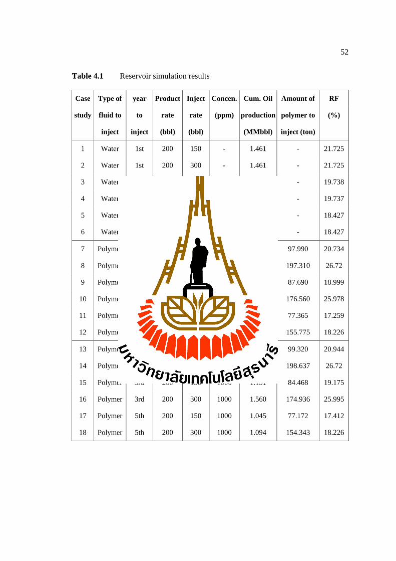
4.1 Reservoir simulation results 52
5.1 Basic assumptions 68
5.2 Cash flow expenditures 69
5.3 Cash flow summary of all case studies 70
6.1 summary of reservoir simulation result 78
6.2 Cash flow summary result 81
LIST OF FIGURES
Figure Page
2.1 Structural stratigraphic in Maesoon oil field (Chananchida, 2012) 6
2.2 Geomorphology and geologic setting of the Fang basin 8
2.3 Oil fields in the Fang basin (Defense Energy Department, 2004) 10
2.4 Interpretation of a seismic profile across the study area with 8 seismic
units Basement and Sq1 to Sq7. On = onlap; Dn = downlap;
Tp = Toplap; Et = erosional truncation; C = Clinoform 11
2.5 Water flooding method showing two water injection wells and
two well productions (Thongsumrit, 2012) 20
2.6 Polymer flooding method (Bradley, 1987) 24
2.7 Molecular structures (Lake, 1989) 26
3.1 Reservoir Structure model 39
3.2 2D Reservoir model 39
3.3 The viscosity versus concentration of polymer solution (Thang, 2005) 45
3.4 The screen factor versus concentration of polymer solution
(Thang, 2005) 46
3.5 Polymer adsorption function graph display result 47
3.6 Polymer shear thinning data graph display result 47
3.7 Polymer solution viscosity function graph display 48
XIII
LIST OF FIGURES (Continued)
Figure Page
3.8 Staggered line drive pattern 50
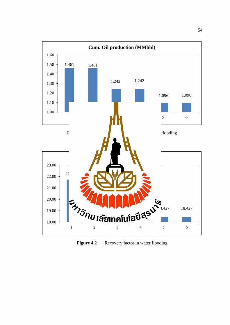
4.1 Cumulative oil production in water flooding 54
4.2 Recovery factor in water flooding 54
4.3 Cumulative oil production in polymer flooding
at concentration 600 ppm 56
4.4 Recovery factor in polymer flooding at concentration 600 ppm 56
4.5 Cumulative oil production in polymer flooding
at concentration 1,000 ppm 57
4.6 Recovery factor in polymer flooding at concentration 1,000 ppm 57
4.7 Cumulative oil production in polymer flooding
at concentration 1,500 ppm 58
4.8 Recovery factor in polymer flooding at concentration 1,500 ppm 58
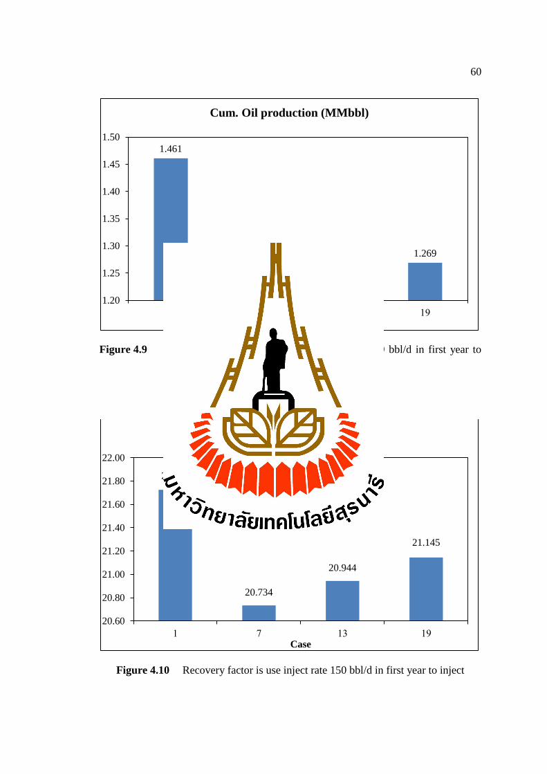
4.9 Cumulative oil production is use inject rate 150 bbl/d
in first year to inject 60
4.10 Recovery factor is use inject rate 150 bbl/d in first year to inject 60
4.11 Cumulative oil production is use inject rate 300 bbl/d
in first year to inject 61
4.12 Recovery factor is use inject rate 300 bbl/d in first year to inject 61
XIV
LIST OF FIGURES (Continued)
Figure Page
4.13 Cumulative oil production is use inject rate 150 bbl/d
in third year to inject 62
4.14 Recovery factor is use inject rate 150 bbl/d in third year to inject 62
4.15 Cumulative oil production is use inject rate 300 bbl/d
in third year to inject 63
4.16 Recovery factor is use inject rate 300 bbl/d in third year to inject 63
4.17 Cumulative oil production is use inject rate 150 bbl/d
in fifth year to inject 64
4.18 Recovery factor is use inject rate 150 bbl/d in fifth year to inject 64
4.19 Cumulative oil production is use inject rate 300 bbl/d
in fifth year to inject 65
4.20 Recovery factor is use inject rate 300 bbl/d in fifth year to inject 65
5.1 Summary of IRR Results, Oil price 85 $/bbl 72
5.2 Summary of PIR Results, Oil price 85 $/bbl 73
5.3 Summary of NPV Results, Oil price 85 $/bbl 74
6.1 Summary of reservoir simulation results 77
6.2 cash flow summary result 80
SYMBOLS AND ABBREVIATIONS
bbl = Barrel
bbl/d = Barrel per day
CAPEX = Capital expense
Disc. = Discount
EOR = Enhanced oil recovery
FCIT = Field polymer injection total
FGIP = Field gas in place
FGPR = Field gas production rate
FGPT = Field gas production total
FOE = Field oil efficiency
FOIP = Field oil in place
FOPR = Field oil production rate
FOPT = Field oil production total
FPR = Field pressure
FVF = Formation volume factor
FWIP = Field water in place
FWPR = Field water production rate
FWPT = Field water production total
GOGD = Gas/oil gravity drainage
HPAM = Hydrolyses polyacrylamides
XVI
SYMBOLS AND ABBREVIATIONS (Continued)
IRR = Internal Rate of Return
Inc. = Income
Inj. = Injection
MSCF/STB = Thousand cubic feet per stock tank barrel
MMBBL = Million barrels
MMSTB = Million stock tank barrels
MMUS$ = Million US dollar
MMUS$/well = Million US dollar per well
MSCF = Thousand cubic feet
NPV = Net present value
OPEX = Operation expense
OOIP = Original oil in place
OWC = Oil/water contact
Pbub = Bubble point pressure
PIR = Profit investment ratio
Ply. = Polymer
ppm = Parts per million
Prod. = Production
RB = Reservoir barrel
RF = Recovery factor
SCF = Standard cubic feet

XVII
SYMBOLS AND ABBREVIATIONS (Continued)
SCFD = Standard cubic feet per day
STB = Stock tank barrel
STOIIP = Stock tank of oil initial in place
TSCF = Trillions of standard cubic feet
Visc. = Viscosity
CHAPTER I
INTRODUCTION
1.1 Rationale and background
Oil recovery operations traditionally have been subdivided into three stages:
primary, secondary and tertiary. The primary production is the initial production
stage, results from the use of natural energy present in a reservoir as main source of
energy for the displacement of oil to producing wells. These natural energy sources
are solution-gas drive, gas-cap drive, natural water drive, fluid and rock expansion,
and gravity drainage. Some artificial lifts may be applied to the primary stage. The
secondary recovery is the second stage of operations, usually was implemented after a
primary production decline. Traditional secondary recovery processes are water
flooding, pressure maintenance, and gas injection to displace oil toward producing
wells. The secondary recovery is now almost synonymous with water flooding. The
tertiary recovery is the third stage of production, is that obtained after water flooding
(or whatever secondary process was used). Because of such situations, the term
“tertiary recovery” fell into disfavor in petroleum engineering literature and the
designation of “Enhanced Oil Recovery” (EOR) became more accepted. The process
is used miscible gases, chemicals, polymer and/or thermal energy to displace
additional oil (Don, Green and Paul Willhite, 1998). The final stage in this study is the
use of polymer flooding in increasing oil production.
2
Thailand oil source countries are smaller and therefore less oil production and
thus adopt water flooding in increasing oil production, but the leading polymer
flooding used very little. This study chose to apply polymer flooding to improve oil
production rate in Thailand. By studying Maesoon oil field which is located in a Fang
oil field study in order to be able to compare the polymer flooding could increase oil
production rate is more than letting the natural production. The simulation software
named “Eclipse100” will be used to design the reservoir pattern and find efficiency
for comparing economics.
1.2 Objectives of the study
This study is intended to inform the work of the polymer flooding that can
improve the performance of oil production in the Maesoon oil field. The program,
namely “Eclipse100” is selected to run the reservoir simulation. This study applies
water and polymer flooding to increase the oil production efficiency in Maesoon oil
fields. The purposes of this study are to (1) Study of water and polymer flooding
(2) Compare the oil production efficiency between water and polymer flooding
(3) Compare the oil production efficiency with a variation of polymer concentration
(4) Evaluate the economics to find the best option for investment and most profitable
in actual operation. After many performance simulation have been run, the efficiency
comparison comes from oil production, and economic principles determine the best
method of Maesoon oil field.
3
1.3 Scopes and limitations of the study
1.3.1 Collect and study data of reservoir in Maesoon oil field.
1.3.2 Find oil reserve and recovery efficiency for water flooding and polymer
flooding by using a simulation program, namely Eclipse100 when changes the
reservoir data, year to inject and rate of injections.
1.3.3 Analyze data and compare the economics of water flooding and polymer
flooding. Determine the best Internal Rate of Return (IRR) and Net Present Value
(NPV).
1.4 Research methodology
1.4.1 Literature review
The review includes details of Maesoon oil field in Fang basin
overview, geological information and stratigraphy, theory of water and polymer
flooding, and case studies of water and polymer flooding. Literature review has been
carried out to study the state-of-art of water and polymer flooding technique.
1.4.2 Data collection and preparation
The sources of reservoir modeling data and some additional geological
data are provided by PTT Exploration and Production Public Company Limited, the
published documents, such as the American Association of Petroleum Geologist
(AAPG), Society of Petroleum Engineers (SPE).
1.4.3 Reservoir simulation
The reservoir simulators or complex computer program that simulate
multiphase displacement processed in two or three dimensions. Reservoir modeling is
4
constructed as a hypothetical model by “ECLIPSE Office E100”, simulation software
must be done in these studies, and then used to predict its dynamic behavior. It solves
the fluid flow equation by using numerical techniques to estimate the saturation
distribution, pressure distribution, and flow of each phase at discrete points in a
reservoir. The reservoir rock properties (porosity, saturation and permeability), the
fluid properties (viscosity and the PVT properties) and other necessary data were
collected and obtained from literature reviewing, concessionaire result and theoretical
assumptions. Data are also based on Maesoon oil field in Fang Basin.
1.4.4 Economic evaluation
Economic evaluation is calculated from the results of reservoir
simulator. This calculated from the reservoir simulator’s results; optimum oil, gas and
water production rate, cumulative oil production recovery, such as capital costs,
operating costs, anticipated revenues, contract terms, fiscal (tax) structure, forecast oil
prices, the timing of the project, and the expectation of the company in the
investment. Different method of water and polymer flooding scenarios were analyzed
to determine the potentially most economically viable projects, time to start water or
polymer injection for each reservoir, were simulated and analyzed to determine the
suitable time that meet the economic criteria for each project.
1.5 Expected results
The following expectative results this study is:
1. Find the oil reserve and recovery efficiency in the Maesoon oil field.
5
2. Find the best method and economically in Maesoon oil field with water
flooding or polymer flooding.
3. Improve knowledge of water and polymer flooding.
4. Assist in planning and energy management, alternative fuel and energy for
utilization in the future.
1.6 Thesis contents
Chapter 1 states the rationale, research objectives, scope and limitations of
the study, research methodology and expected result. Chapter 2 summarizes results
of the literature review of Fang Basin and Mae Soon oil field overview, water and
polymer flooding and reservoir simulation method. Chapter 3 describes the reservoir
simulation data preparations, model characteristics, classification and case study
description. Chapter 4 illustrates the result of water and polymer flooding simulation
model. Chapter 5 analyzes result of simulation model in term of economic
considerations. Conclusion and discussion of future research needs are given in
Chapter 6. Appendix A illustrates simulation data. Appendix B illustrated polymer
data. Economic data are shown in Appendix C. Reservoir simulation result are shown
in Appendix D.
6
CHAPTER II
LITERLATURE REVIEW
2.1 Maesoon oil field
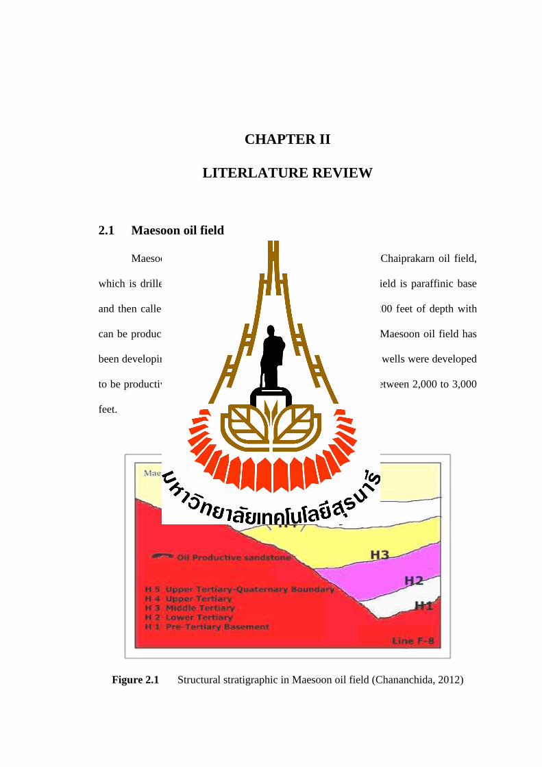
Maesoon oil field was found and developed following Chaiprakarn oil field,
which is drilled for exploration in 1963. Crude oil in the oil field is paraffinic base
and then called Maesoon crude oil. There is an oil layer at 2,200 feet of depth with
can be produced oil about 50 bbl per day. From 1963 to 2010 Maesoon oil field has
been developing. There were 84 exploration wells and about 33 wells were developed
to be productive well. Almost of oil layer have a depth range between 2,000 to 3,000
feet.
Figure 2.1 Structural stratigraphic in Maesoon oil field (Chananchida, 2012)
7
Maesoon oil field is a potential source of petroleum; oil-drilling exploration
and development holes, the most oil production in Fang district, Chiang Mai
Province.
2.2 Fang basin
The Fang Oilfield is located in Fang intermontane basin, Northern Thailand. It
is approximately 150 kilometer north of Chiang Mai or 850 kilometer from Bangkok,
the capital of Thailand. The surface area is approximately 600 square kilometer
(width 12 and length 50 kilometer), probably the smallest intermontane basin in
which petroleum has been discovered in the country. The basin lies NE-SW with an
elongated shape and is surrounded by older formations of rocks from Cambrian and
Igneous rocks to more recent sediments. The highest peak is around 2,000 meter and
the basin is about 450 meter above mean sea level.
People living in the area are Thai citizens and also more than 10 groups of
minority hill tribes including Chinese, Mong, Muser, E-koe, Palong, Dai Yai, Karen,
Yao, Wa, Lisor and local northern people with different dialects and cultures.
The area is hilly with green mountain forest and beautiful nature. As such,
Fang is one of the most attractive places for both Thai and foreign tourists who visit
all year long. During December and January, some days the temperature might drop
down to 5-10°C and sometimes even as low as 0°C on the peak of Doi Angkang. Such
climatic conditions are rarely found in other places of the country.

8
Figure 2.2 Geomorphology and geologic setting of the Fang basin
Agriculture and commerce are the main economies in the region. Among most
popular fruits from this area are lychees and honey oranges which are very tasty. On
the top of Doi Angkang where the Royal King’s project station is located, many
plants, floras and vegetables from cold countries are planted aimed at reducing drug
activities previously common in the area. The main oil production operated from the
sandstone of the Mae Sod Formation in the Mae Soon, San Sai, Nong Yao, Sam Jang
and Ban Thi structures. Most oil fields in Fang basin were belonging to and operated
9
by the Department of Defence Energy, and produced by natural flows which now are
expelled by low differential pressures and finally resulted in lower production
efficiency. Present day, the sucker rod pumping units is used to improve oil recovery
of these oil fields. These oil fields have a long history of operation and production in
some tracts has decreased, with many wells currently exhibiting water cut increases.
In order to reduce operating expenditures on electricity for sucker rod pumping unit,
intermit operation is selected to study in this research. The methods of intermit
operation have been to build up the pressure in a well by shutting in well for 12 hours
and then open hole for normal flow for 12 hours. As a result, work hours of sucker
rod pump are reduced. Moreover, the useful life of sucker rod pumping unit could
also be extended and this can also reduce its maintenance and spare part costs. The
total production from the Fang basin is approximately 9 million barrels (MMbbl) from
the following 7 reservoirs since early 1960 to the present day.
I. Chaiprakarn Reservoir (abandoned 1984), II. Maesoon Reservoir, III.
Pongnok Reservoir (abandoned 1985), IV. Sansai Reservoir, V. Nongyao Reservoir,
VI. Sanjang Reservoir, VII. Banthi Reservoir.
2.3 Statigraphy
2.3.1 Stratigraphy of Fang basin
Based on the characteristics of seismic reflections, seven seismic
sequences have been identified and described successively upward as follows.
10
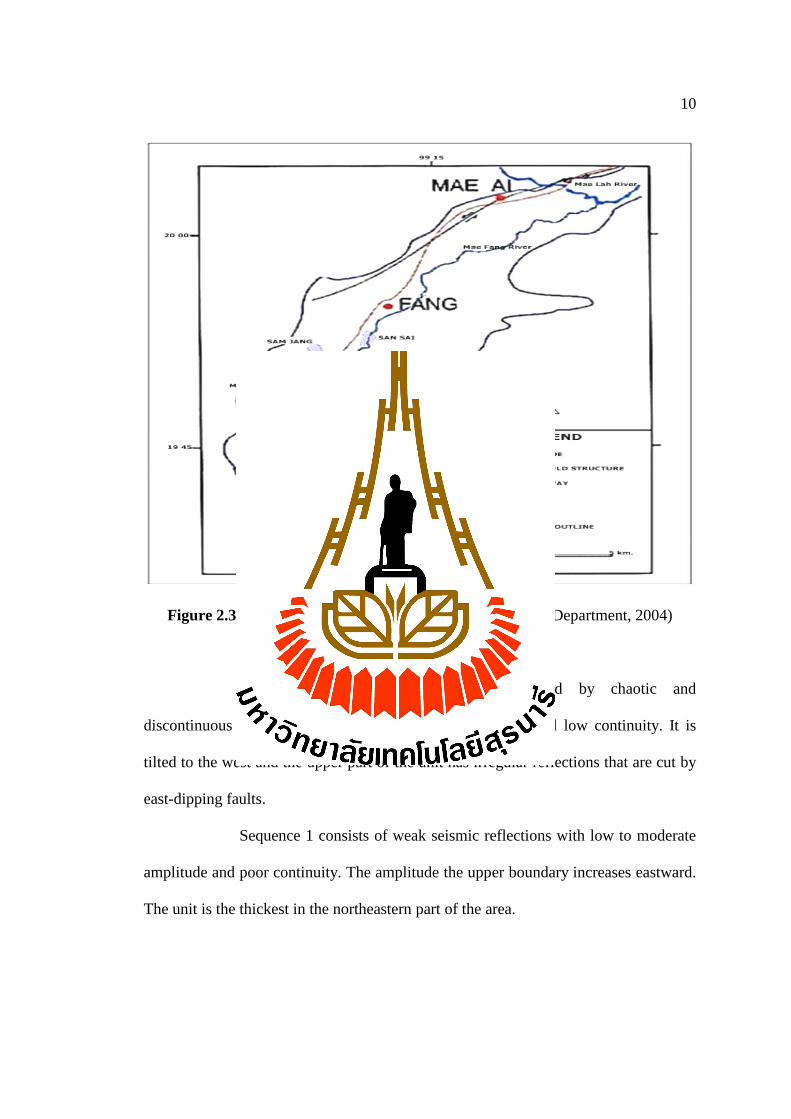
Figure 2.3 Oil fields in the Fang basin (Defense Energy Department, 2004)
The Pre-Tertiary basement is characterized by chaotic and
discontinuous reflections with moderate to low amplitude and low continuity. It is
tilted to the west and the upper part of the unit has irregular reflections that are cut by
east-dipping faults.
Sequence 1 consists of weak seismic reflections with low to moderate
amplitude and poor continuity. The amplitude the upper boundary increases eastward.
The unit is the thickest in the northeastern part of the area.
11
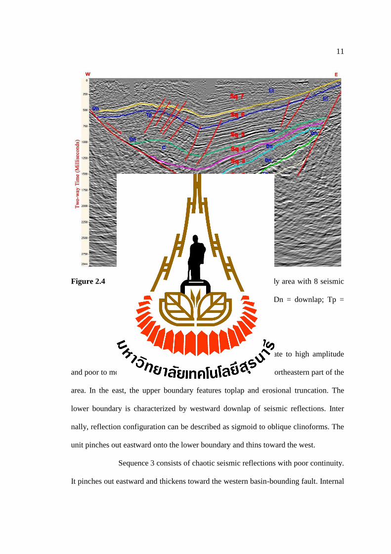
Figure 2.4 Interpretation of a seismic profile across the study area with 8 seismic
units Basement and Sq1 to Sq7. On = onlap; Dn = downlap; Tp =
Toplap; Et = erosional truncation; C = Clinoform
Sequence 2 the seismic reflections have moderate to high amplitude
and poor to moderate continuity. The unit is the thickest in the northeastern part of the
area. In the east, the upper boundary features toplap and erosional truncation. The
lower boundary is characterized by westward downlap of seismic reflections. Inter
nally, reflection configuration can be described as sigmoid to oblique clinoforms. The
unit pinches out eastward onto the lower boundary and thins toward the west.
Sequence 3 consists of chaotic seismic reflections with poor continuity.
It pinches out eastward and thickens toward the western basin-bounding fault. Internal
12
reflections are sub-parallel with moderate to low amplitude and onlap onto the lower
boundary. The upper boundary is a concordant reflection with moderate to strong
amplitude.
Sequence 4 has similar seismic characteristics to those of Sequences 2
and 3. It is a prograding unit that thins eastward and thickens toward the western
basin-bounding fault. The seismic reflections within the unit have high amplitude.
Sequence 5 can be separated into five subsequences: 5I, 5H, 5G, 5F
and 5E, successively upward. Most reservoirs of the Fang oil fields are located within
Sequence 5. The seismic reflections in the unit are sub- parallel and have moderate to
high amplitude with moderate to good continuity. The reflections onlap onto the
lower boundary at the western and eastern margins of the basin. The upper boundary
is characterized by erosional truncation in the east and toplap in the west. Strong
reflections occur near the basin margins and become less prominent in the basin
centre.
Sequence 6 consists of seismic reflections inside the unit with low to
medium amplitude and moderate continuity. The reflections onlap onto the lower
boundary at both basin margins. The upper boundary is characterized by erosional
truncation over most of the area.
Sequence 7 consists of seismic reflections with low amplitude and
moderate to poor continuity. The reflections are better resolved in the basin centre. At
the basin margin, they appear to onlap onto the lower boundary. In the western half of
the basin, erosional truncation characterizes the upper part of the unit.
13
2.3.2 Depositional Environments
Depositional environments of the basin fills were interpreted from
analysis of seismic reflections in combination with well data. This information is
considered crucial in predicting the possibility and suitability of a prospected area.
Depositional environments for the seven seismic units are discussed as follows.
In general all of the seismic units represent sediment that was
deposited in a continental environment including purely fluvial and lacustrine
conditions as well as the transition between the two regimes.
Based on well information, the Pre-Tertiary basement consists of
weathered andesite and Permian limestone. The sandstone in Sequence 1 has been
described as poorly sorted, angular and rich in feldspar and rock fragments. This
information and its seismic characteristics of low to moderate amplitude and poor
continuity indicate that the unit was probably deposited in a fluvial environment with
the sediment sources at the basin margins. The upper boundary has very strong
amplitude and corresponds to bituminous shale and lignite, which are regarded as
good source rocks in the eastern part of the Fang basin. Well information reveals that
Sequence 2 consists of a series of sandstone inter-bedded with shale. The sandstone is
grayish and well- sorted with sub-angular to sub-rounded grains. The alternation of
sandstone and shale provides seismic reflections with moderate to high amplitudes
and poor to moderate continuity. Clinoform seismic configuration indicates a
westward-directed prograding unit.
The sub-parallel to chaotic reflections with poor continuity of
Sequence 3 can be interpreted to represent deposition in a low energy environment or

14
a lake where mud dominated. The strong reflection at the upper unit boundary
corresponds to coal that indicates a possible swampy environment, especially along
the lake margins.
Clinoform configuration in seismic profiles of Sequence 4 indicates a
westward directed prograding unit. Strong reflections within the unit correspond to
alternation of sandstone and shale. Data from wells show that the sandstone is
moderately sorted with angular to sub-rounded grains. Sequence 5 comprises
sandstone inter-bedded with shale. The sandstone forms reservoirs in the western part
and the eastern part of the Fang basin. The internal reflections are sub-parallel and
onlap onto both the western and eastern basin margins. The strong seismic amplitudes
at the basin margins that decrease toward the basin centre can be interpreted as a
transition from alternating sandstone and shale in the shallower part to dominantly
shale in the deeper part of the basin. This information suggests that the sediment was
supplied by sources on the basin flanks.
Sequence 6 consists of dominantly shale inter-bedded by minor
sandstone. The upper boundary of the unit shows erosional truncation that can be
interpreted as an unconformity corresponding to a seismic reflection with have
moderate to low amplitude and moderate to low continuity. Sequence 7 is the
youngest sequence. Seismic reflections in this sequence have low amplitude and
moderate to poor continuity that probably correspond to alternating sandstone and
shale layers. At the basin margins, they appear to onlap onto the lower boundary and
the reflections are better resolved in the basin centre. Therefore, the sediment has
been interpreted as being supplied from the basin margins. In the western half of the

15
basin, erosional truncation characterizes the upper part of the unit. This erosion was
probably a result of local or regional uplift of the basin (Nuntajun, 2009).
2.3.3 Subsurface Lithostratigraphy
From the geological data there are 2 major formations from the upper
zone of Maefang formation to lower zones of Maesod formation as follows:
Maefang Formation (Quaternary + Recent)
The post-rift of Maefang formation overlies discordantly above the
Maesod formation. The thickness of the Maefang formation from the surface varies
from 1,000-1,800 feet. The minimum thickness is found on top of the Maesoon
structure. The thickness will increase down dip from the crest of the structure.
Maefang formation is mainly composed of coarse clastic sediments of
soil, lateritic sands, loose sands, gravels, cobbles and pebbles, carbonized woods and
clay on the top and towards the basin edge. Sizes of sands vary from coarse to very
coarse grains, roundness from angular to sub-angular, poorly sorted and inter-bedded
with reddish clays. While down dip towards the central basin clay-shale and arkosic
sandstone are inter-bedded. This formation overlies discordantly with the Maesod
formation. The Maefang formation shows energetic alluvial and fluvial deposits.
Maesod Formation (Middle Tertiary)
The Maesod formation is composed of brown to gray shale, yellowish
mud stone generally inter-bedded with sand and sandstone with a series of channels of
sand paleodelta and fluvial sand.
Basal conglomerate lies unconformity with Pre-Tertiary rocks and
continues with sequences of lacustrine shale and mudstone. The color of the
16
sediments indicates a reducing environment in the central, deeper part of the basin
while an oxidizing environment develops in the shallow part of basin. Organic shale
in the central part of the basin plays an important role as a potential source of rocks.
The upper part of the Tertiary sediments is inter-bedded with 4 packages of sand
which are important reservoir rocks in the Fang basin. Only 2 packages of sands have
been proven to be producing sands. The sand thickness varies from 1-10 meter.
The thickness of the Maesod formation varies from the margin of the
basin towards the centre of the basin. At the Maesoon structure the thickness is
approximately 3,500 feet or total thickness (Maefang + Maesod formation) 5,000 feet
from the surface. Seismic interpretations indicate that the thickest part of the Maesod
formation might reach up to 8,000 feet at the deepest part of the basin.
Basement (Pre-Tertiary)
The age of the basement of the Fang basin ranges from Mesozoic
continental clastics to Cambrian marine clastics.
2.3.4 Oil Reservoir
Within the Fang basin, all productions come from the Maesod
formation. The current producing reservoirs are distributed into widespread sections
of the sorted sands and coarse clastics in some cases.
Reservoir distribution
Generally, inter-bedded sand and sandstones in the upper zones of the
Maesod formation are dominant reservoir rocks in the Maesoon reservoir and others.
The sand member which gives the lowest production includes 4 layers
of sand. The thickness of each sand layer varies from 5-45 feet. The depth of this sand
17
is about 2,386-2,487 feet which is the main producer of wells. The thickest part of this
sand is in a North-South direction. Porosity decreases towards the margin of the
reservoir.
The sand member gives the highest production includes 5 sands, 5-15
feet in thickness for each sand, with a total thickness of about 55 feet. The depth is
about 2,160-2,255 feet. Most of the old wells are from this sand 2,300 feet in depth.
The thickness of the sand varies from place to place. The trend in thickness North-
South is 55 feet and decreasing to 10-15 feet at the edge of reservoir.
Reservoir Properties
Cores analysis from some wells shows interesting results of porosity
up to 25%, permeability higher than 200 milliDarcy (mD), some loose clastics as high
as 2,000-3,000 mD found in the well IF 26 Table 2.1 Reservoir properties.
Table 2.1 Reservoir properties
Well Depth
(ft)
Permeability
(mD)
Porosity
(%)
Fluid saturation (%) Density
(gm/cc) Oil (Sor) Wat (Sw)
BS-110 2,755 231 25.7 6.1 54.4 2.67
IF-26 1) 2,581 2,390 25.4 17.5 33.0 2.65
2) 2,587 3,440 26.7 20.5 34.7 2.64
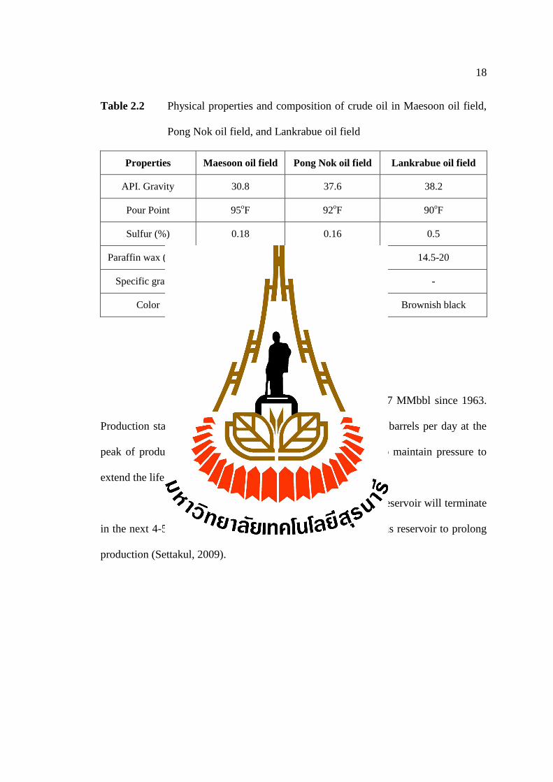
Fluid Properties
Physical properties of oil from Maesoon, Pongnok, and Lankrabreau
are quite similar with a very high content of paraffin wax up to 18% shown on the
Table 2.2
18
Table 2.2 Physical properties and composition of crude oil in Maesoon oil field,
Pong Nok oil field, and Lankrabue oil field
Properties Maesoon oil field Pong Nok oil field Lankrabue oil field
API. Gravity 30.8 37.6 38.2
Pour Point 95oF 92
oF 90
oF
Sulfur (%) 0.18 0.16 0.5
Paraffin wax (%wt) 18 18.62 14.5-20
Specific gravity 0.872 0.873 -
Color Brownish black Brownish black Brownish black
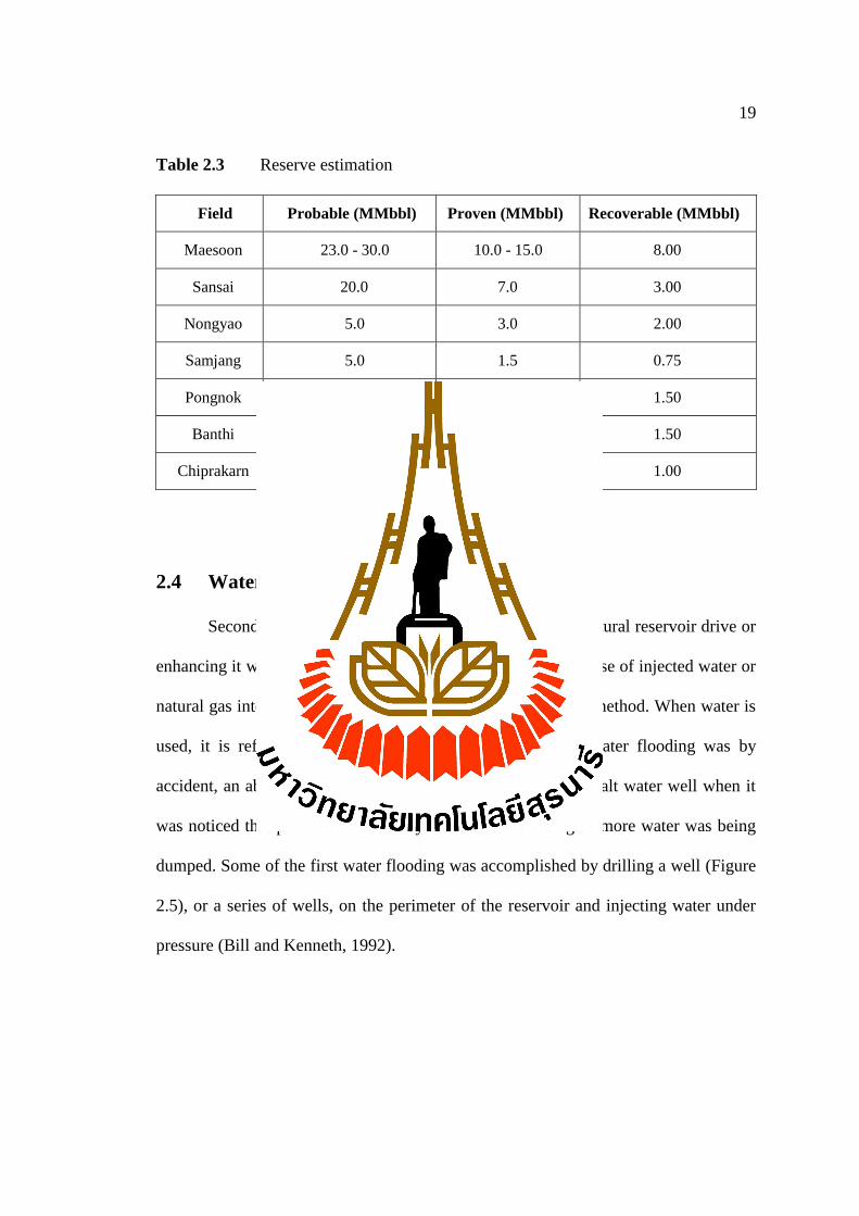
Reserve Estimation
The Maesoon reservoir has produced a total of 7 MMbbl since 1963.
Production started from 100 barrel per day up to nearly 1,000 barrels per day at the
peak of production (Table 2.3). The mature reservoir needs to maintain pressure to
extend the life of the reservoir.
From the decline curve the life of the Maesoon reservoir will terminate
in the next 4-5 years. Secondary recovery will be needed for this reservoir to prolong
production (Settakul, 2009).
19
Table 2.3 Reserve estimation
Field Probable (MMbbl) Proven (MMbbl) Recoverable (MMbbl)
Maesoon 23.0 - 30.0 10.0 - 15.0 8.00
Sansai 20.0 7.0 3.00
Nongyao 5.0 3.0 2.00
Samjang 5.0 1.5 0.75
Pongnok 6.0 3.0 1.50
Banthi 8.0 3.0 1.50
Chiprakarn 4.5 1.5 1.00
2.4 Water flooding
Secondary recovery actually consists of replacing the natural reservoir drive or
enhancing it with an artificial, or induced drive. Generally the use of injected water or
natural gas into the production, reservoir is the most common method. When water is
used, it is referred to as water flooding. The first known water flooding was by
accident, an abandoned oil well was being used as a disposal salt water well when it
was noticed that production of nearby wells was increasing as more water was being
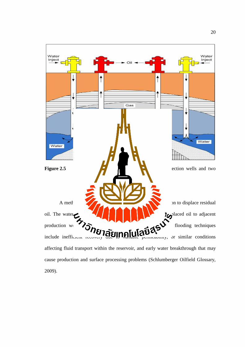
dumped. Some of the first water flooding was accomplished by drilling a well (Figure
2.5), or a series of wells, on the perimeter of the reservoir and injecting water under
pressure (Bill and Kenneth, 1992).
20
Figure 2.5 Water flooding method showing two water injection wells and two
well productions (Thongsumrit, 2012)
A method used water to inject into the reservoir formation to displace residual
oil. The water from injection wells physically sweeps the displaced oil to adjacent
production wells. Potential problems associated with water flooding techniques
include inefficient recovery due to variable permeability, or similar conditions
affecting fluid transport within the reservoir, and early water breakthrough that may
cause production and surface processing problems (Schlumberger Oilfield Glossary,
2009).
21
2.5 Case study of water flooding
2.5.1 Jay-LEC Field:
The Jay-LEC field has produced from the Smackover carbonate and
Norphlet sand formations at depth about 15,400 feet. An oil/water contact is located at
a sub-sea depth of 15,480 ft. More than 90% of the oil in place are in Smackover. The
reservoir study indicated that the natural water drive would not be an effective source
of reservoir energy. Thus, water flood was selected among other possible processes to
maintain pressure for increasing oil recovery. The water flooding plan in Smackover
formation was developed by using a two dimensional (2D) simulation to compare
alternative flooding schemes. Four water flood plans were evaluated: (1) peripheral
flood, (2) five spot pattern (3) a 3:1 staggered line drive pattern and (4) a combination
of peripheral wells and five spot patterns. From the results of the 2D simulator
indicated that the peripheral flood was not effective. For the remaining three water
flooding plans, the 3:1 staggered line drive plan was recovered more than 200
MMbbl. The 3:1 plan yielded 9.8 MMbbl incremental oil recoveries over the five spot
plan and 14.4 MMbbl over the combination pattern. Moreover the 3:1 plan also has
advantages for development plan and economic potential (Willhite, 1986).
2.5.2 Fahud field
A fracture model was constructed for the Natih-E reservoir unit of the
Fahud Field in northern Oman. The fracture model indicates that the current gas/oil
gravity drainage (GOGD) recovery mechanism is an inefficient oil recovery method
for a large part of the lower Natih-E. The optimum well pattern for a water flood
development within two Natih-E subunits is proposed on the basis of simulation
22
results. Nicholls et al. (2000) studies the fracture modeling and they expected that the
oil recovery is increased from 17 percent under GOGD to 40 percent of the water
flood. A fracture model that includes information from well production and injection
performance, borehole-image data, structural map, and fault data has been constructed
foe the Natih-E containing sparse and widely spaced fractures. A pilot water injection
cell of two horizontal procedures and one injector well oriented parallel to the
bedding strike has shown that water injection is a viable alternative to GOGD
(Nicholls et. al., 2000).
2.5.3 Sirikit oil field
The oil fields in the Sirikit area are situated within Phitsanulok basin.
The basin has an areal extent in order of 6,000 square kilometers formed as a result of
the relative movement of the Shan Tai and Indonesian Blocks. The Sirikit oilfield is
geologically very complex. The geological complexity is a product of the multiphased
structural history and the interaction between faulting and deposition through time.
The water flooding is one of the successful projects which have been developed in the
Sirikit oilfields. The water flood project started as early as 1983. A small pilot project
in a small area of LKU-E block was designed to test the viability of injecting water
into the complex sand shale inter-bedded layers of the LanKrabu formations. It was
proved that the pilot test could maintain pressure under a non-fracturing condition. So
it was indicated that the water flooding of LanKrabu reservoir was feasible. The water
flooding project had studied again during 1993-1994. It gave a boost to the confidence
in recovery factor of the field, which increased over 20 percent for the first time. The
discovery of oil in Pradu Tao and Yom reservoirs during 1997-1998 gave another
23
upgrade to the recovery factor to a level of around 25 percent. The implement of the
previous water flood project encountered many operational difficulties, but proved
water flood to be a technically viable secondary recovery technique in the Sirikit
complex reservoirs. Reviews and studies of reservoir performances and simulations of
the Sirikit reservoirs indicated that a reserve volume is recoverable only through the
water flood of the Sirikit reservoirs. Recent disappointing results of new infill wells
confirmed that the plans to drill hundreds of infill wells would not be as effective as
water flooding. With the advanced of computer modeling techniques compared to 10
years ago, the confidence of successfully implementing water flooding projects in the
Sirikit Field has been reviewed (Wongsirasawad, 2002).
2.6 Polymer flooding
Polymer flooding is a type of chemical flooding to control drive-water
mobility and fluid flow patterns in reservoirs. Polymer-long, chainlike, high-weight
molecules have three important oil recovery properties. They increase water viscosity,
decrease effective rock permeability and are able to change their viscosity with the
flow rate. Small amounts of water-dissolved polymer increase the viscosity of water.
This higher viscosity slows the progress of the water flow through a reservoir and
makes it less likely to bypass the oil in low permeability rock (Gerding, 1986).
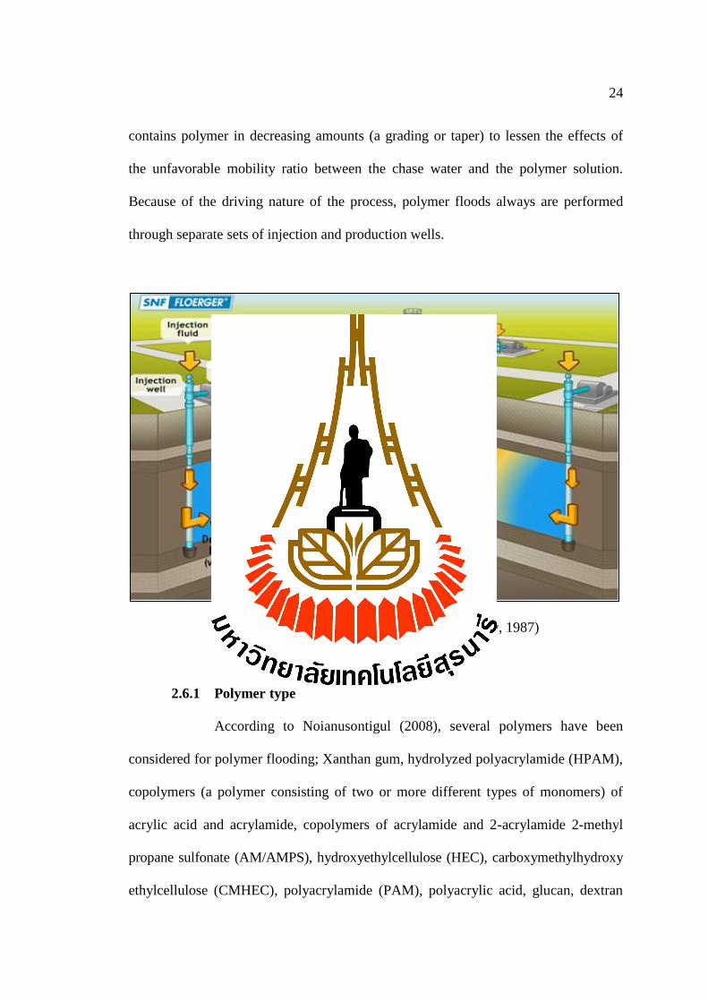
The figure 2.6 show a schematic of a typical polymer flood injection
sequence: a preflush is usually consists of a low salinity brine; an oil bank is injected
by polymer; a fresh water buffer to protect the polymer solution from backside
dilution; and the last are chased or drive water. Many times the freshwater buffer
24
contains polymer in decreasing amounts (a grading or taper) to lessen the effects of
the unfavorable mobility ratio between the chase water and the polymer solution.
Because of the driving nature of the process, polymer floods always are performed
through separate sets of injection and production wells.
Figure 2.6 Polymer flooding method (Bradley, 1987)
2.6.1 Polymer type
According to Noianusontigul (2008), several polymers have been
considered for polymer flooding; Xanthan gum, hydrolyzed polyacrylamide (HPAM),
copolymers (a polymer consisting of two or more different types of monomers) of
acrylic acid and acrylamide, copolymers of acrylamide and 2-acrylamide 2-methyl
propane sulfonate (AM/AMPS), hydroxyethylcellulose (HEC), carboxymethylhydroxy
ethylcellulose (CMHEC), polyacrylamide (PAM), polyacrylic acid, glucan, dextran
25
polyethylene oxide (PEO), and polyvinyl alcohol. Although only the first three have
actually been used in the field, there are many potentially suitable chemicals, and
some may prove to be more effective than those new used. Polymer can be
commercially categorized in two types:
2.6.1.1 Polyacrylamides (PAM)
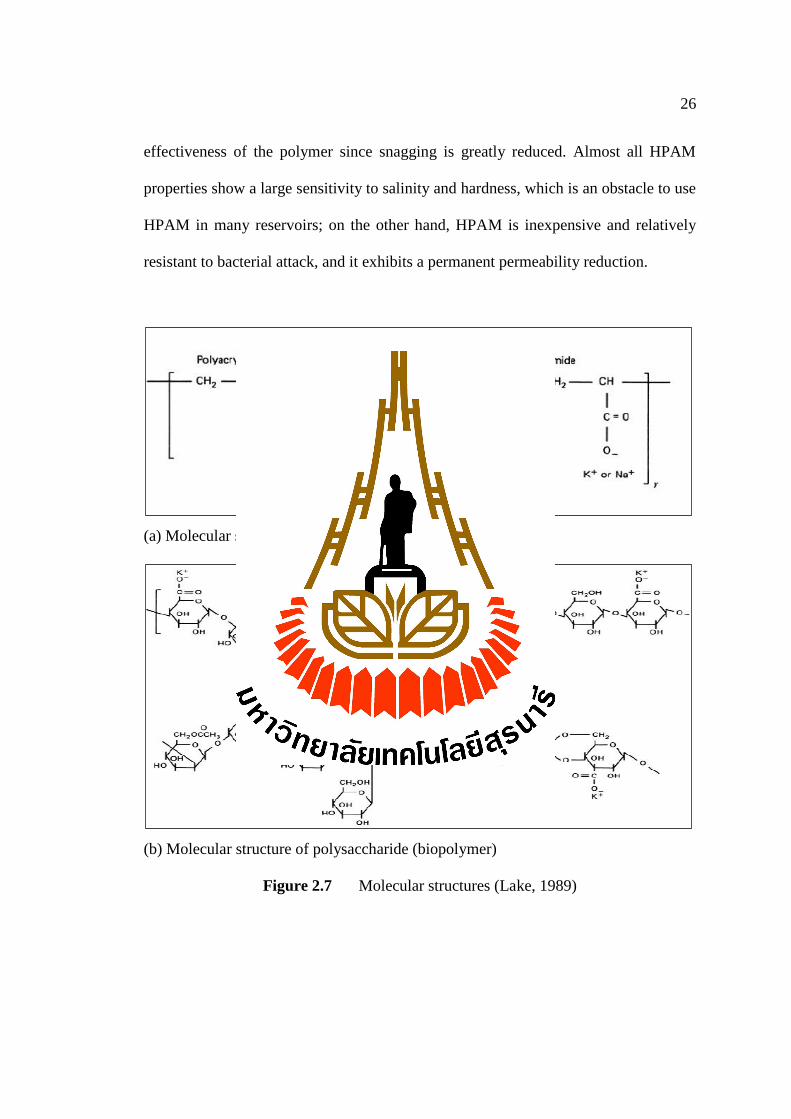
These polymers’ monomeric unit is the acrylamide molecule
(Figure 2.7a). When used in polymer flooding, polyacrylamides have undergone
partial hydrolysis, which causes anionic (negatively charged) carboxyl (-COO-) to be
scattered along the backbone chain. For this reason these polymers are called partially
hydrolyses polyacrylamides (HPAM). Typical degrees of hydrolysis are 30-35% of
the acrylamide monomers; hence the HPAM molecule is negatively charged, which
accounts for many of its physical properties. This degree of hydrolysis has been
selected to optimize certain properties such as water solubility, viscosity, and
retention. If hydrolysis is too small, the polymers will not be water-soluble. If it is too
large, the polymers will be too sensitive to salinity and hardness.
The viscosity-increasing feature of HPAM lies in its large
molecular weight. This feature is accentuated by the anionic repulsion between
polymer molecules and between segments in the same molecule. The repulsion causes
the molecule in solution to elongate and snug on those similarly elongated, an effect
that accentuates the mobility reduction at higher concentrations.
If the brine salinity or hardness is high, this repulsion is greatly
decreased through ionic shielding since the freely rotating carbon-carbon bonds allow
the molecule to coil up. The shielding causes a corresponding decrease in the
26
effectiveness of the polymer since snagging is greatly reduced. Almost all HPAM
properties show a large sensitivity to salinity and hardness, which is an obstacle to use
HPAM in many reservoirs; on the other hand, HPAM is inexpensive and relatively
resistant to bacterial attack, and it exhibits a permanent permeability reduction.
(a) Molecular structure of polyacrylamide
(b) Molecular structure of polysaccharide (biopolymer)
Figure 2.7 Molecular structures (Lake, 1989)
27
2.6.1.2 Polysaccharides
Another widely used polymer, a biopolymer, is xanthan gum
(corn sugar gum).This kind of polymer is formed from the polymerization of
saccharide molecule (Figure 2.7b), a bacterial fermentation process. This process
leaves substantial debris in the polymer product that must be removed before the
polymer is injected. The polymer is also susceptible to bacterial attack after it has
been introduced into the reservoir. The disadvantages are also offset by the
insensitivity of polysaccharide properties to brine salinity and hardness. The
polysaccharide molecule is relatively non-ionic and, therefore, free of the ionic
shielding effects of HPAM. Polysaccharides are more branched than HPAM, and the
oxygen-ringed carbon bond does not rotate fully; hence the molecule increase brine
viscosity by snagging and adding a more rigid structure to the solution.
Polysaccharides do not exhibit a permeability reduction. Molecular weights of
polysaccharides are generally around 2 million.
From the study in thermal and rheological of polysaccharides,
at 55oC and 65ºC an increase in viscosity values was observed. This behavior is
interesting for polymer flooding operations into the reservoir, temperatures are in this
level or still higher, the cost of polymer could be reduced. Xanthan is supplied as a
dry powder or as a concentrated broth. It is often chosen for a field application when
no fresh water is available for flooding. Some permanent shear loss of viscosity could
occur for polyacrylamide, but not for polysaccharide at the wellbore. It is an
advantage in offshore operations.
28
HPAM is less expensive per unit amount than polysaccharides,
but between compared on a unit volume of mobility reduction, particularly at high
salinities, the costs are close enough so that the preferred polymer for given
application is site specific (Manning et. al., 1983).
2.6.2 Polymer flow behavior in porous media
2.6.2.1 Polymer retention
According to Maheshwari (2011), retention of polymer in a
reservoir includes adsorption, mechanical trapping, and hydrodynamic retention.
Adsorption refers to the interaction between polymer molecules and the solid surface.
This interaction causes polymer molecules to be bound to the surface of the solid,
mainly by physical adsorption, and hydrogen bonding. Mechanical entrapment and
hydrodynamic retention are related and occur only in flow through porous media.
Retention by mechanical entrapment occurs when larger polymer molecules become
lodged in narrow flow channels. The level of polymer retained in a reservoir rock
depends on permeability of the rock, nature of the rock (sandstone, carbonate,
minerals, or clays), polymer type, polymer molecular weight, polymer concentration,
brine salinity, and rock surface.
2.6.2.2 Inaccessible pore volume
When size of polymer molecules is larger than some pores in a
porous medium, the polymer molecules cannot flow through those pores. The volume
of those pores that cannot be accessed by polymer molecules is called inaccessible
pore volume (IPV). The inaccessible pore volume is a function of polymer molecular
29
weight, medium permeability, porosity, salinity, and pore size distribution. In extreme
cases, IPV can be 30% of the total pore volume.
2.6.2.3 Permeability reduction and the resistance factor
Polymer adsorption/retention causes the reduction in apparent
permeability. Therefore, rock permeability is reduced when a polymer solution is
flowing through it, compared with the permeability when water is flowing. This
permeability reduction is defined by the permeability reduction factor:
p
(2.1)
where Rk = Permeability reduction factor
kw = Rock permeability when water flows
kp = Rock permeability when aqueous polymer solution flows
The resistance factor is defined as the ratio of mobility of water
to the mobility of a polymer solution flowing under the same conditions.
p
(2.2)
where Rf = Resistance factor
µo, µw = Viscosity of oil and water, cp
The residual resistance factor is the ratio of the mobility of
water before to that after the injection of polymer solution.
30
r
p
a (2.3)
where Rrf = Residual resistance factor
Residual resistance factor is a measure of the tendency of the
polymer to adsorb and thus partially block the porous medium. Permeability reduction
depends on the type of polymer, the amount of polymer retained, the pore-size
distribution, and the average size of the polymer relative to pores in the rock.
2.6.2.4 Relative permeability in polymer flooding
Some of the researchers have proved from their experiments
that polymer flooding does not reduce residual oil saturation in a micro scale. The
polymer function is to increase displacing fluid viscosity and thus to increase sweep
efficiency. Also, fluid viscosities do not affect relative permeability curves. Therefore,
it is believed that the relative permeability in polymer flooding and in water flooding
after polymer flooding are the same as those measured in water flooding before
polymer flooding.
2.6.2.5 Polymer rheology in porous media
The rheological behavior of fluids can be classified as
Newtonian and Non-Newtonian. Water is a Newtonian fluid in that the flow rate
varies linearly with the pressure gradient, thus viscosity is independent of flow rate.
Polymers are Non-Newtonian fluids.
Rheological behavior can be expressed in the terms of apparent
viscosity which can be defined as:
31
(2.4)
where = shear stress
= shear rate
The apparent viscosity of polymer solutions used in EOR
processes decreases as shear rate increases. Fluids with this rheological characteristic
are said to be shear thinning. Materials that exhibit shear thinning effect are called
pseudo plastic. Polysaccharides such as Xanthan are not shear sensitive and even high
shear rate is employed to Xanthan solutions to obtain proper mixing, while
polyacrylamides are more shears sensitive. Most significant change in polymer
mobility occurs near the wells where fluid viscosities are large.
2.7 Case study of polymer flooding
2.7.1 Feasibility study of secondary polymer flooding in Henan Oilfield
Henan oil field is the second largest oil field in Henan Province,
People's Republic of China. It is located in Nanyang region. The field was discovered
in 1970s. It has accumulated proven oil reserves of 2.7 billion tons. It is operated by
Sinopec Henan Oilfield Company, a subsidiary of Sinopec (Wikipedia, 2012). During
1996 to 2006, polymer flooding was implemented in Henan Oilfield, with average 70
mPa.s o crude oil viscosity and reservoir temperature o 55˚C, polymer o 0.42 PV to
0.44 PV was injected with above 8% of enhanced recovery. In the next water
flooding, water cut rises rapidly, and part of the lower permeability zone was not
32
developing, therefore it is necessary to employ relay technology to retain yield. On
the other hand, the total produced degree is less than 35%, that is to say, more than
65% of residual crude oil still exists in underground, and both vertical and plane
heterogeneity are serious. Therefore, according to characteristic of crude oil and
formation, a series of laboratory experiments to study the feasibility of secondary
polymer flooding were carried, including microscopic mechanism study and
macroscopic physical modeling. In addition, the polymer concentration must be
optimized to ensure recovery effect and economics. Filed trial with above optimum
parameters was implemented. Water cuts decreased from 92% to 83%, and
cumulative increased crude oil of above 50,000 tons.
2.7.2 Polymer flooding in a large field in south oman
This large sandstone field was discovered in 1956s. The oil is heavy
(22°API) and viscous (90 cp). The field is highly heterogeneous with sand diamictite
and shale bodies. However, the main reservoir units the net-sand/gross-reservoir ratio
approaches 1.0 and the permeability can be many darcies.
The crude oil and the resulting poor mobility ratio with the displacing
water, the achievable recovery by water flooding were estimated at 20 to 30%. The
Phase-I project consists of polymer injection in 27 existing injection wells, with the
aim to increase recovery by approximately 10% of the targeted area. Polymer
injection takes place through 20 inverted nine spot patterns, four inverted five spot
patterns all with vertical injectors and three patterns with horizontal injectors. Initial
polymer injection took place in February 2010, and the project was fully
commissioned in April 2010. The polymer injection rate is approximately 13,000
33
m3/d in 15 cp polymer viscosity at the wellhead. This project is the first full scale
polymer plant in Oman and the Middle East, and is one of very few full scale polymer
applications in the world (Faisal, Henri, and Pradeep, 2012).
2.7.3 Reduced well spacing combined with polymer flooding improves
oil recovery from marginal reservoirs
In continental, multilayer, heterogeneous sandstone oil fields, some
reservoirs with poor connectivity and low permeability have low recovery factors.
The low degree of layer connection and inner-layer interferences lead to poor water
flooding efficiency, to improve oil recovery and increase recoverable reserves, infill
wells were drilled to improve reservoir connectivity and a polymer solution was
injected. Average incremental oil per day for a single well was 1.83 times original
production. Water cut decreased 10.2%, and oil recovery increased more than 10%
(Sui, and Bai, 2006).
2.8 Recovery efficiency
A key factor in the design of a water or polymer flooding is the estimation of
the oil recovery. This factor indicates the portion of the initial oil in place that can be
economically recovered by water injection. In equation form, the oil recovery by
water or polymer flooding can be expressed by
Np = N * EA * EV * ED (2.5)
where Np = Cumulative Water flooding Recovery, bbl
N = Oil In Place at start of injection, bbl
34
EA = Areal Sweep Efficiency, Fraction
EV = Vertical Sweep Efficiency, Fraction
ED = Displacement Efficiency, Fraction
2.8.1 The displacement efficiency
The displacement efficiency (ED) is the fraction of movable oil that has
been displaced from the swept zone at any given time or pore volume injected.
Because an injection fluid (water or polymer) will always leave behind some residual
oil, ED will always be less than 1, the displacement efficiency can be expressed by
olume o oil at start o lood - emaining oil volume
olume o oil at start o lood (2.6)
Pore volume
oi
oi
- Pore volume o
o
Pore volume oi
oi
(2.7)
or
oi
oi
- o
o
oi
oi
(2.8)
where oi = volumetric average oil saturation at the beginning of the
water or polymer flooding, where the average pressure is p1,
fraction
o = volumetric average oil saturation at a particular point during
the water or polymer flooding
Boi = oil FVF at pressure is pressure is p1, bbl/STB
35
Bo = oil FVF at a particular point during the water or polymer
flooding, bbl/STB
When the oil saturation in the PV swept by water or polymer flooding
is reduced to the residual saturation (Sor),
- or
oi
oi
o (2.9)
This becomes
- or
oi (2.10)
where Sor = residual oil, fraction
oi = volumetric average oil saturation at the beginning of the
water or polymer flooding, where the average pressure is p1,
fraction
2.8.2 The areal sweep efficiency
The areal sweep efficiency (EA) is defined as the fraction of the total
flood pattern that is contacted by the displacing fluid. It increases steadily with
injection from zero at the start of the flood until breakthrough occurs, after which EA
continues to increase at a slower rate.
The areal sweep efficiency depends basically on the following three
main factors:
36
- Mobility ratio (M)
- Flood pattern
- Cumulative fluid injected
2.8.3 The vertical sweep efficiency
The vertical sweep efficiency (EV) is defined as the fraction of the
vertical section of the pay zone that is the injection fluid. This particular sweep
efficiency depends primarily on (1) the mobility ratio and (2) total volume injected.
As a consequence of the non-uniform permeability, any injected fluid will tend to
move through the reservoir with an irregular front. In the more permeable portions,
the injected water will travel more rapidly than in the less permeable zone.
2.8.4 The mobility ratio
The mobility of a fluid is the effective relative permeability of that
fluid divided by its viscosity. For an injection scheme, the mobility ratio (M) is the
ratio of the mobility of the displacing fluid behind the flood front to that of the
displaced fluid ahead of the flood front.
The mobility of any fluid λ is defined as the ratio of the effective
permeability of the fluid to the fluid viscosity,
λo o
o
ro
o (2.11)
λ
r
(2.12)
λg g
g
rg
g (2.13)
where λo, λw, λg = mobility of oil, water, and gas, respectively
37
µo, µw, µg = viscosity of oil, water, and gas, cp
ko, kw, kg = effective permeability to oil, water, and gas,
respectively
kro, krw = relative permeability to oil, water, and gas,
respectively
k = absolute permeability
for water flooding,
λ
λo
r
o
ro (2.14)
simplifying gives
r
ro
o
(2.15)
I mobility ratio ≤ , oil is capable o traveling ith a velocity equal
to or more than that water. If mobility ratio M > 1, water is capable of traveling faster
than oil. As the water is pushing the oil through the reservoir, some of oil will be by
passed.
CHAPTER III
RESERVOIR SIMULATION
3.1 General
Reservoir simulation is a technique in which a computer-based mathematical
representation of the reservoir is constructed and then use to predict its dynamic
behavior. Simulation is the only way to describe quantitatively the flow of multi-
phases in a heterogeneous reservoir having a production schedule determined not only
by the properties of the reservoir, but also by market demand, investment strategy,
and government regulations. The reservoir is a gridded up into a number of grid
blocks. The reservoir rock properties (porosity, saturation and permeability) and the
fluid properties (viscosity and PVT data) are applied for each grid block.
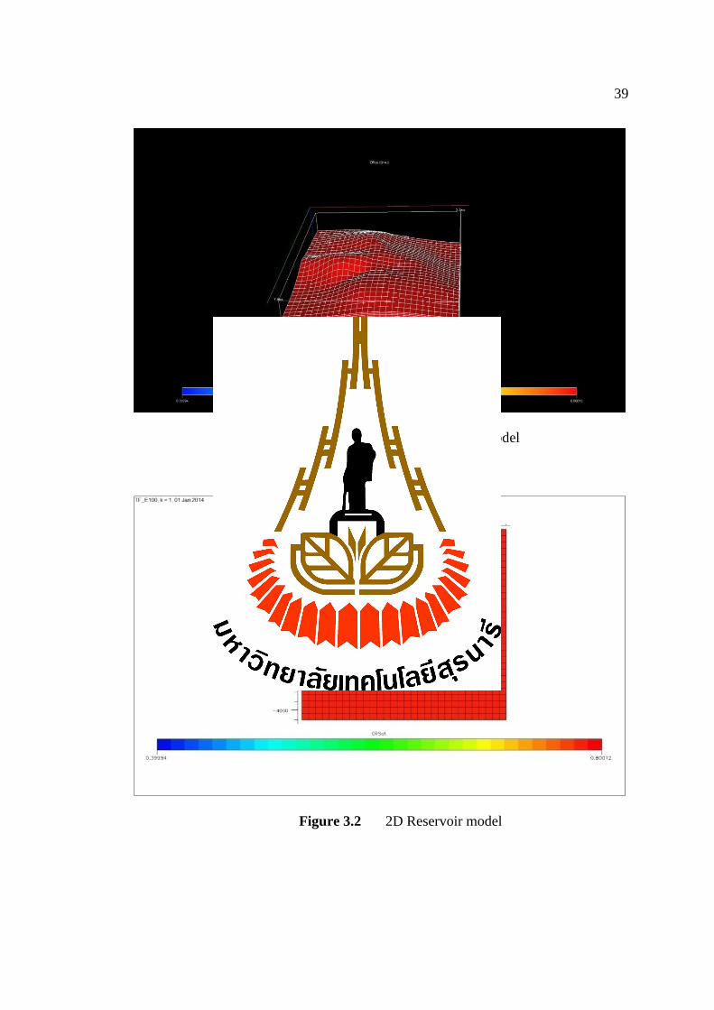
3.2 Reservoir simulation model
This study used dead-oil reservoir simulation by Eclipse Office E100 to
simulate all types of reservoir (primary, secondary and tertiary productions) which
based on available data on Mae Soon oil field and some of data assumptions. The
structure of reservoir simulation is shown in figure 3.1 to 3.2 and the detail summarize
as follows:
39
Figure 3.1 Reservoir Structure model
Figure 3.2 2D Reservoir model
40
- Model dimension (long, wide, thick) 4200, 4200, 105 feet
- Scale grid (x, y, z) 30, 30, 6 (5,400 grid blocks)
- Structure style Monocline
- Unit Field
- Geometry type Conner Point
- Grid type Cartesian
3.3 Data input for the reservoir model
The data input in the reservoir model are received from available data of Mae
Soon oil field data. The main input data section of the simulation are Grid section,
PVT section, SCAL section, Fluid Initialization section and Schedule section. Some
data are assumed for using in this study because they are not available for Mae Soon
data.
3.3.1 Grid section data
The data input in this section is used keyword type Properties and
geometry. Properties is input data active grid block, permeability distribution,
porosity and net to gross thickness ratios. Geometry is an input data grid block
coodinate line and grid block corners. The data for Grid section is following:
- Net-to-gross ratio 0.18 – 1.00
41
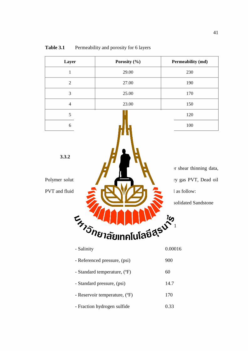
Table 3.1 Permeability and porosity for 6 layers
Layer Porosity (%) Permeability (md)
1 29.00 230
2 27.00 190
3 25.00 170
4 23.00 150
5 21.00 120
6 19.00 100
3.3.2 PVT section data
The PVT section data are used keyword Polymer shear thinning data,
Polymer solution viscosity function, Water PVT properties, Dry gas PVT, Dead oil
PVT and fluid Density. The data input for PVT section are detail as follow:
- Rock type of reservoir Consolidated Sandstone
- Oil gravity, (API Oil) 35.1
- Gas gravity, (SG Air = 1) 0.881
- Bubble point pressure, (psi) 14.7
- Salinity 0.00016
- Referenced pressure, (psi) 900
- Standard temperature, (ºF) 60
- Standard pressure, (psi) 14.7
- Reservoir temperature, (ºF) 170
- Fraction hydrogen sulfide 0.33
42
- Fraction carbon dioxide 0.03
- Fraction nitrogen 0.04
3.3.3 Scal section data
The SCAL section data use keyword Polymer adsorption function, Oil
saturation, Gas saturation, Water saturation and Polymer rock properties. The data
input for PVT section are detail as follow:
- Initial water saturation 0.2
- Oil saturation 0.1
- Gas saturation 0.04
- Polymer adsortion function 0.35
The Table A.1, A.2 of PVT Dry gas property and Dead oil PVT
property are shown in Appendix A.
3.3.4 Fluid initialization section data
Initialization refers to the initial conditions of the simulation. The
initial conditions are defined by specifying the OWC (Oil-Water contact) depths and
the pressure at a known depth. ECLIPSE uses this information in conjunction with
much of the information from previous stages to calculate the initial hydrostatic
pressure gradients in each zone of the reservoir model and allocate the initial
saturation of each phase in every grid cell prior to production and injection. The data
of calibration are as follows:
- Datum depth, (feet) 3,850
- Pressure at datum depth, (psi) 1,800
- Water/Oil contact depth, (feet) 3,875
43
3.3.5 Well data about schedule section data
Well data provides well and completion locations, production and
injection rates of wells and other data, the use keyword Well specifiation, Well
completion data, Production well control, Production well economic limits, etc. The
well data which use in producing wells and injection wells as following;
- Diameter of well bore (feet) 0.71
- Skin factor -1
- Effective Kh (mD) 250
- Perforation of production zone (layer) 1st - 6th
- Perforation of injection zone (layer) 1st - 6th
3.3.6 Type of polymer for injection
The Xanthan Gum (XCD) polymer concentration 1,000 and 1,500 ppm
is used in this study. XCD polymer has a good salt-resistance. The reservoir has a
high temperature this polymer can increase the water viscosity but the mobility ratio
between polymer solution and oil will be decrease. This study is comparison different
of polymer concentration for use is the best case and development for each reserved
sizes of the reservoir. Recovery efficiency and economic evaluations are more
favorable than the others concentrations. Data of polymer solution for injection.
According to Kanarak (2011), Data is collected from the result of
laboratory testing on polymer properties. The experiment is to examine the polymer
properties at high temperature. The tests that were carried out are:
1. Heat-resistance of polymer
2. Screen factor of polymer
44
The polymer properties to be determined are:
1. The viscosity versus concentration of polymer solution with changed
temperature.
2. The screen factor versus concentration of polymer solution with
changed temperature.
The testing was carried out at different polymer concentrations: 600,
1,200, 1,800, 2,400 and 3,000 ppm, dissolved both with the freshwater and brine.
Testing results for polymer properties
According to Thang (2005), the measurement parameters of XCD
polymer solution at the different concentrations before and after heating are presented
in Table B1 in Appendix B. The viscosity and screen factor versus concentration with
changed temperature. The test of polymer solution have considerable loss of viscosity
(plastic and apparent viscosity) and screen factor after heated polymer up to 150º C in
the different times. Especially in the polymer samples with low concentration (600
ppm), the capability of increased viscosity and screen factor were almost lost. The
problem which has to use high polymer concentration will make increasing the cost
price of method and therefore it makes reducing the economic efficiency.
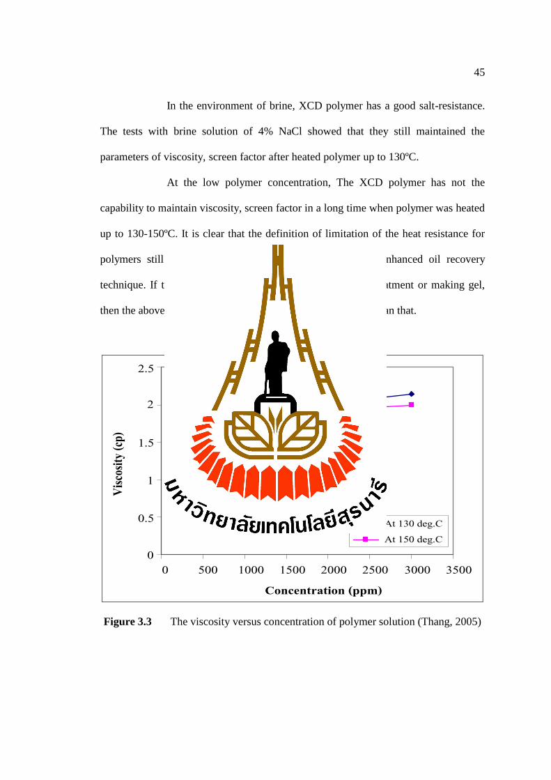
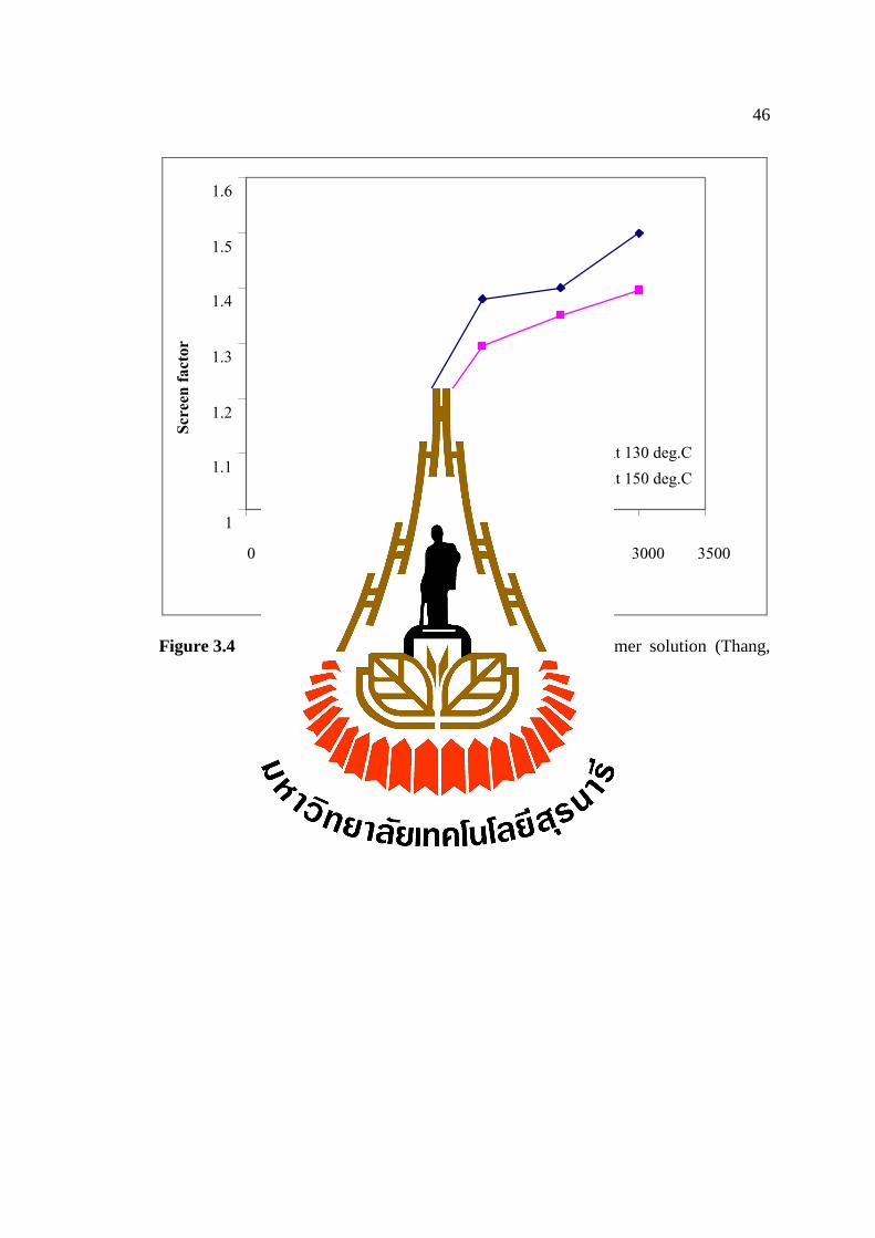
The capability to maintain of plastic viscosity versus the concentration
after heating up XCD polymer solution to 150ºC is presented in Figure 3.3 and 3.4.
The parameters of plastic viscosity, screen factor high increase with the increasing
concentration up to value as 1,200 ppm. At the higher values of concentration more
than 1,200 ppm, this increase now were become less and the curves levels off.
45
In the environment of brine, XCD polymer has a good salt-resistance.
The tests with brine solution of 4% NaCl showed that they still maintained the
parameters of viscosity, screen factor after heated polymer up to 130ºC.
At the low polymer concentration, The XCD polymer has not the
capability to maintain viscosity, screen factor in a long time when polymer was heated
up to 130-150ºC. It is clear that the definition of limitation of the heat resistance for
polymers still depends on the purpose of using it in the enhanced oil recovery
technique. If the polymer are used for the purpose of well treatment or making gel,
then the above solutions can be satisfied up to 150ºC or more than that.
0
0.5
1
1.5
2
2.5
0 500 1000 1500 2000 2500 3000 3500Concentration (ppm)
Viscos
ity (c
p)
At 130 deg.CAt 150 deg.C
Figure 3.3 The viscosity versus concentration of polymer solution (Thang, 2005)
46
1
1.1
1.2
1.3
1.4
1.5
1.6
0 500 1000 1500 2000 2500 3000 3500Concentration (ppm)
Scre
en fa
ctor
At 130 deg.C At 150 deg.C
Figure 3.4 The screen factor versus concentration of polymer solution (Thang,
2005)
47
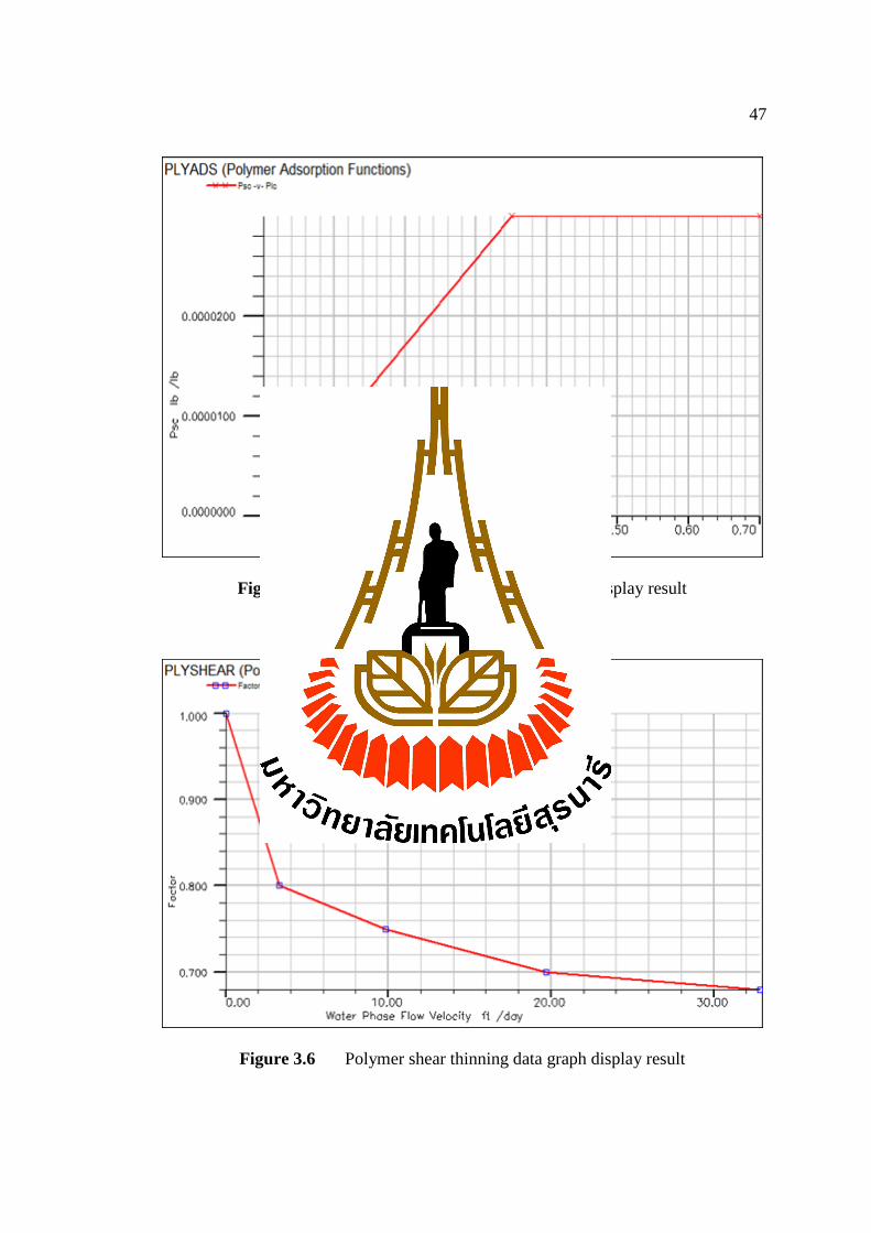
Figure 3.5 Polymer adsorption function graph display result
Figure 3.6 Polymer shear thinning data graph display result
48
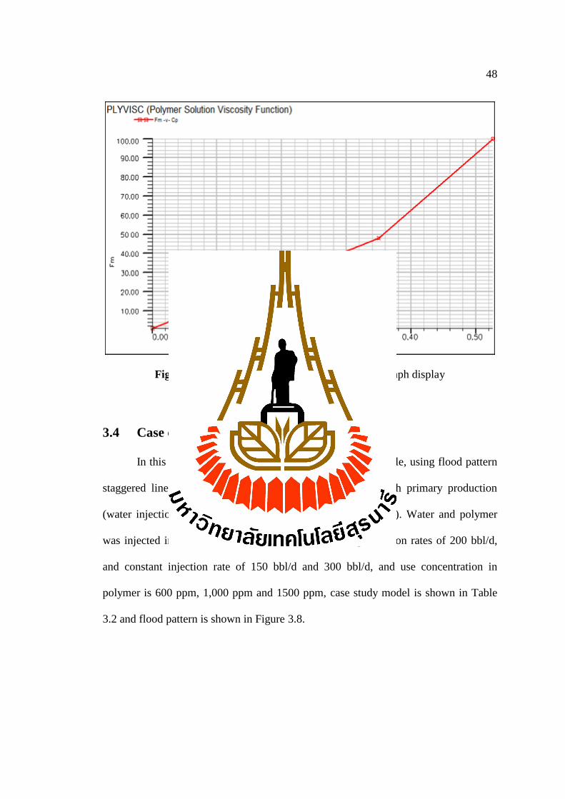
Figure 3.7 Polymr solution viscosity function graph display
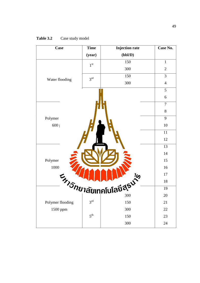
3.4 Case of study
In this study the reservoir is the monocline structure style, using flood pattern
staggered line drive to compare the result of production with primary production
(water injection) and secondary production (polymer injection). Water and polymer
was injected in the 1st, 3rd and 5th with the constant production rates of 200 bbl/d,
and constant injection rate of 150 bbl/d and 300 bbl/d, and use concentration in
polymer is 600 ppm, 1,000 ppm and 1500 ppm, case study model is shown in Table
3.2 and flood pattern is shown in Figure 3.8.
49
Table 3.2 Case study model
Case
Time
(year)
Injection rate
(bbl/D)
Case No.
Water flooding
1st
150
300
1
2
3rd
150
300
3
4
5th
150
300
5
6
Polymer flooding
600 ppm
1st 150
300
7
8
3rd 150
300
9
10
5th 150
300
11
12
Polymer flooding
1000 ppm
1st
3rd
5th
150
300
150
300
150
300
13
14
15
16
17
18
Polymer flooding
1500 ppm
1st
3rd
5th
150
300
150
300
150
300
19
20
21
22
23
24
50
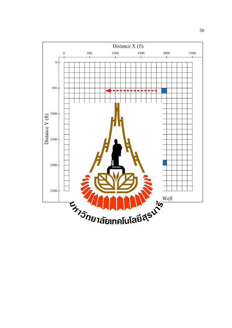
Figure 3.8 Staggered line drive pattern
51
CHAPTER IV
RESERVOIR SIMULATION RESULTS
4.1 Reservoir simulation result
This chapter shows reservoir simulation results of the total 24 cases studies,
comprising of graphs with 2 phases of fluids (oil and water) because there is little gas
production in dead oil reservoir. The graphs show field fluid in place (a volume in the
reservoir), field cumulative production (production efficiency), field production rate
(production profile), field pressure, field oil efficiency and field polymer injection
total. Result from running simulations of the 24 case studies to explain fluid behavior
water flooding and polymer flooding methods. The result is shown in Table 4.1.
52
Table 4.1 Reservoir simulation results
Case Type of year Product Inject Concen. Cum. Oil Amount of RF
study fluid to to rate rate (ppm) production polymer to (%)
inject inject (bbl) (bbl)
(MMbbl) inject (ton)
1 Water 1st 200 150 - 1.461 - 21.725
2 Water 1st 200 300 - 1.461 - 21.725
3 Water 3rd 200 150 - 1.242 - 19.738
4 Water 3rd 200 300 - 1.242 - 19.737
5 Water 5th 200 150 - 1.096 - 18.427
6 Water 5th 200 300 - 1.096 - 18.427
7 Polymer 1st 200 150 600 1.245 97.990 20.734
8 Polymer 1st 200 300 600 1.604 197.310 26.72
9 Polymer 3rd 200 150 600 1.140 87.690 18.999
10 Polymer 3rd 200 300 600 1.559 176.560 25.978
11 Polymer 5th 200 150 600 1.036 77.365 17.259
12 Polymer 5th 200 300 600 1.093 155.775 18.226
13 Polymer 1st 200 150 1000 1.257 99.320 20.944
14 Polymer 1st 200 300 1000 1.604 198.637 26.72
15 Polymer 3rd 200 150 1000 1.151 84.468 19.175
16 Polymer 3rd 200 300 1000 1.560 174.936 25.995
17 Polymer 5th 200 150 1000 1.045 77.172 17.412
18 Polymer 5th 200 300 1000 1.094 154.343 18.226
53
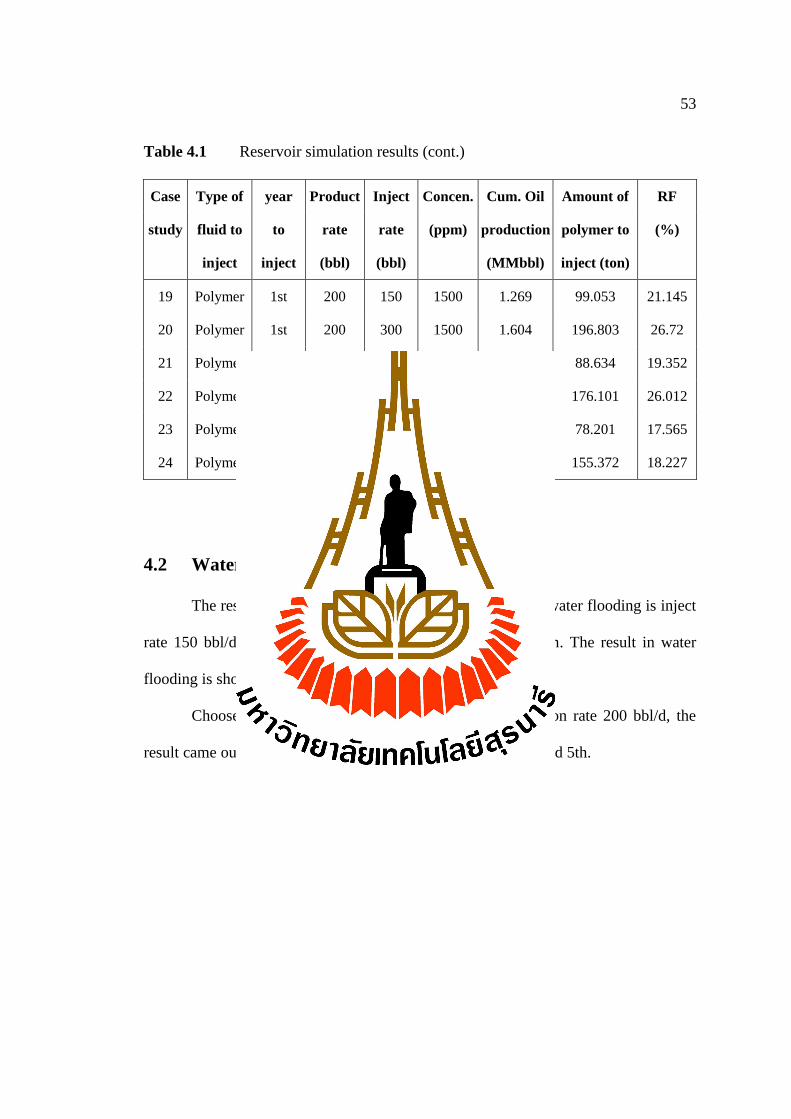
Table 4.1 Reservoir simulation results (cont.)
Case Type of year Product Inject Concen. Cum. Oil Amount of RF
study fluid to to rate rate (ppm) production polymer to (%)
inject inject (bbl) (bbl)
(MMbbl) inject (ton)
19 Polymer 1st 200 150 1500 1.269 99.053 21.145
20 Polymer 1st 200 300 1500 1.604 196.803 26.72
21 Polymer 3rd 200 150 1500 1.161 88.634 19.352
22 Polymer 3rd 200 300 1500 1.561 176.101 26.012
23 Polymer 5th 200 150 1500 1.054 78.201 17.565
24 Polymer 5th 200 300 1500 1.093 155.372 18.227
4.2 Water flooding result
The reservoir simulation result is a comparison case in water flooding is inject
rate 150 bbl/d and 300 bbl/d in year inject to 1st, 3rd and 5th. The result in water
flooding is shown Figure 4.1 and 4.2.
Choose case 1 in water flooding because use production rate 200 bbl/d, the
result came out with similar values. In use inject year 1st, 3rd and 5th.
54
Figure 4.1 Cumulative oil production in water flooding
Figure 4.2 Recovery factor in water flooding
1.461 1.461
1.242 1.242
1.096 1.096
1.00
1.10
1.20
1.30
1.40
1.50
1.60
1 2 3 4 5 6
Cum. Oil production (MMbbl)
21.725 21.725
19.738 19.737
18.427 18.427
18.00
19.00
20.00
21.00
22.00
23.00
1 2 3 4 5 6
RF (%)
55
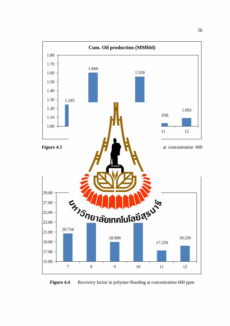
4.3 Polymer flooding result
The reservoir simulation result is a comparison case in polymer flooding is
concentration 600 ppm is inject rate 150 bbl/d and 300 bbl/d at production rate 200
bbl/d. In use inject year 1st, 3rd and 5th. The result is shown in Figure 4.3 and Figure
4.4.
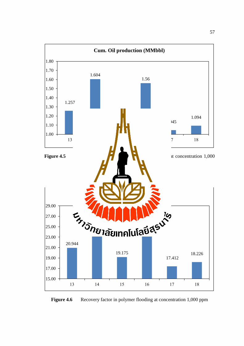
The reservoir simulation result is a comparison case in polymer flooding is
concentration 1,000 ppm is inject rate 150 bbl/d and 300 bbl/d at production rate 200
bbl/d. In use inject year 1st, 3rd and 5th. The result is shown in Figure 4.5 and Figure
4.6.
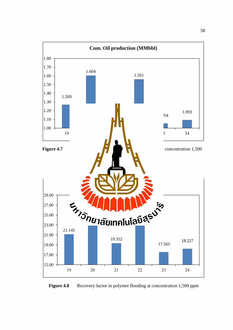
The reservoir simulation result is a comparison case in polymer flooding is
concentration 1,500 ppm is inject rate 150 bbl/d and 300 bbl/d at production rate 200
bbl/d. In use inject year 1st, 3rd and 5th. The result is shown in Figure 4.7 and Figure
4.8.
56
Figure 4.3 Cumulative oil production in polymer flooding at concentration 600
ppm
Figure 4.4 Recovery factor in polymer flooding at concentration 600 ppm
1.245
1.604
1.14
1.559
1.036
1.093
1.00
1.10
1.20
1.30
1.40
1.50
1.60
1.70
1.80
7 8 9 10 11 12
Cum. Oil production (MMbbl)
20.734
26.72
18.999
25.978
17.259 18.226
15.00
17.00
19.00
21.00
23.00
25.00
27.00
29.00
7 8 9 10 11 12
RF (%)
57
Figure 4.5 Cumulative oil production in polymer flooding at concentration 1,000
ppm
Figure 4.6 Recovery factor in polymer flooding at concentration 1,000 ppm
1.257
1.604
1.151
1.56
1.045 1.094
1.00
1.10
1.20
1.30
1.40
1.50
1.60
1.70
1.80
13 14 15 16 17 18
Cum. Oil production (MMbbl)
20.944
26.72
19.175
25.995
17.412 18.226
15.00
17.00
19.00
21.00
23.00
25.00
27.00
29.00
13 14 15 16 17 18
RF (%)
58
Figure 4.7 Cumulative oil production in polymer flooding at concentration 1,500
ppm
Figure 4.8 Recovery factor in polymer flooding at concentration 1,500 ppm
1.269
1.604
1.161
1.561
1.054 1.093
1.00
1.10
1.20
1.30
1.40
1.50
1.60
1.70
1.80
19 20 21 22 23 24
Cum. Oil production (MMbbl)
21.145
26.72
19.352
26.012
17.565 18.227
15.00
17.00
19.00
21.00
23.00
25.00
27.00
29.00
19 20 21 22 23 24
RF (%)
59
4.4 Comparison result in change year to inject in water and
polymer flooding
The all case use injection rate 150 bbl/d in first year to inject, the case use
comparison is case 1, case 7, case 13 and case 19. The result is shown Figure 4.9 and
Figure 4.10. Choose case 1 is water flooding injection rate 150 bbl/d and production
rate 200 bbl/d are best in production oil.
The all case use injection rate 300 bbl/d in first year to inject, the case use
comparison is case 2, case 8, case 14 and case 20. The result is shown in Figure 4.11
and Figure 4.12.
The all case use injection rate 150 bbl/d in third year to inject, the case use
comparison is case 3, case 9, case 15 and case 21. The result is shown in Figure 4.13
and Figure 4.14.
The all case use injection rate 300 bbl/d in third year to inject, the case use
comparison is case 4, case 10, case 16 and case 22. The result is shown in Figure 4.15
and Figure 4.16.
The all case use injection rate 150 bbl/d in fifth year to inject, the case use
comparison is case 5, case 11, case 17 and case 23. The result is shown in Figure 4.17
and Figure 4.18.
The all case use injection rate 300 bbl/d in fifth year to inject, the case use
comparison is case 6, case 12, case 18 and case 24. The result is shown in Figure 4.19
and Figure 4.20.
60
Figure 4.9 Cumulative oil production is use inject rate 150 bbl/d in first year to
inject
Figure 4.10 Recovery factor is use inject rate 150 bbl/d in first year to inject
1.461
1.245 1.257
1.269
1.20
1.25
1.30
1.35
1.40
1.45
1.50
1 7 13 19 Case
Cum. Oil production (MMbbl)
21.725
20.734
20.944
21.145
20.60
20.80
21.00
21.20
21.40
21.60
21.80
22.00
1 7 13 19 Case
RF (%)
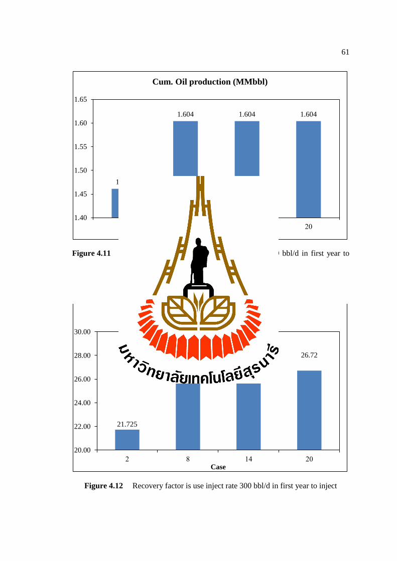
61
Figure 4.11 Cumulative oil production is use inject rate 300 bbl/d in first year to
inject
Figure 4.12 Recovery factor is use inject rate 300 bbl/d in first year to inject
1.461
1.604 1.604 1.604
1.40
1.45
1.50
1.55
1.60
1.65
2 8 14 20 Case
Cum. Oil production (MMbbl)
21.725
26.72 26.72
26.72
20.00
22.00
24.00
26.00
28.00
30.00
2 8 14 20 Case
RF (%)
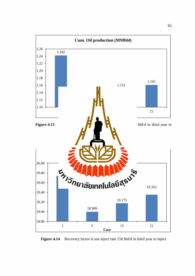
62
Figure 4.13 Cumulative oil production is use inject rate 150 bbl/d in third year to
inject
Figure 4.14 Recovery factor is use inject rate 150 bbl/d in third year to inject
1.242
1.14 1.151
1.161
1.10
1.12
1.14
1.16
1.18
1.20
1.22
1.24
1.26
3 9 15 21 Case
Cum. Oil production (MMbbl)
19.738
18.999
19.175
19.352
18.80
19.00
19.20
19.40
19.60
19.80
20.00
3 9 15 21 Case
RF (%)
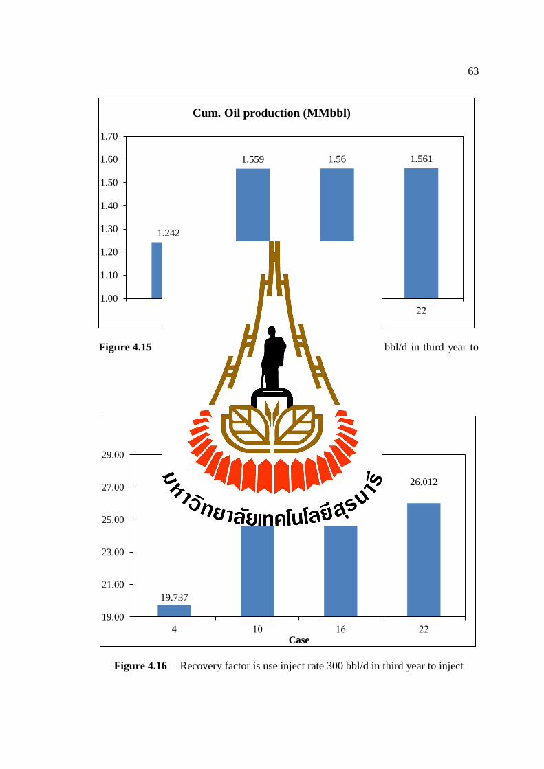
63
Figure 4.15 Cumulative oil production is use inject rate 300 bbl/d in third year to
inject
Figure 4.16 Recovery factor is use inject rate 300 bbl/d in third year to inject
1.242
1.559 1.56 1.561
1.00
1.10
1.20
1.30
1.40
1.50
1.60
1.70
4 10 16 22 Case
Cum. Oil production (MMbbl)
19.737
25.978 25.995
26.012
19.00
21.00
23.00
25.00
27.00
29.00
4 10 16 22 Case
RF (%)
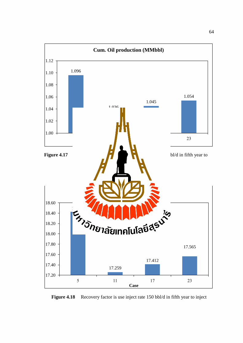
64
Figure 4.17 Cumulative oil production is use inject rate 150 bbl/d in fifth year to
inject
Figure 4.18 Recovery factor is use inject rate 150 bbl/d in fifth year to inject
1.096
1.036
1.045
1.054
1.00
1.02
1.04
1.06
1.08
1.10
1.12
5 11 17 23 Case
Cum. Oil production (MMbbl)
18.427
17.259
17.412
17.565
17.20
17.40
17.60
17.80
18.00
18.20
18.40
18.60
5 11 17 23 Case
RF (%)
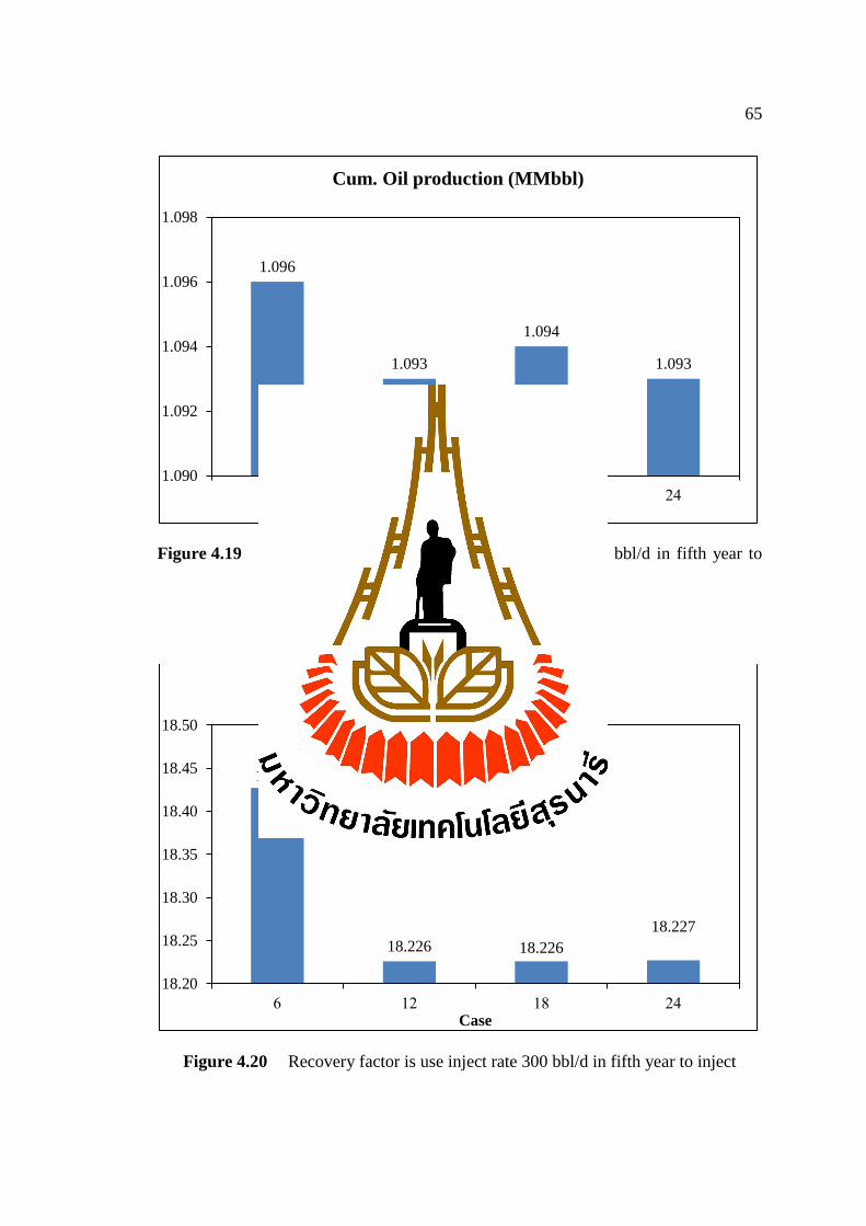
65
Figure 4.19 Cumulative oil production is use inject rate 300 bbl/d in fifth year to
inject
Figure 4.20 Recovery factor is use inject rate 300 bbl/d in fifth year to inject
1.096
1.093
1.094
1.093
1.090
1.092
1.094
1.096
1.098
6 12 18 24 Case
Cum. Oil production (MMbbl)
18.427
18.226 18.226
18.227
18.20
18.25
18.30
18.35
18.40
18.45
18.50
6 12 18 24 Case
RF (%)
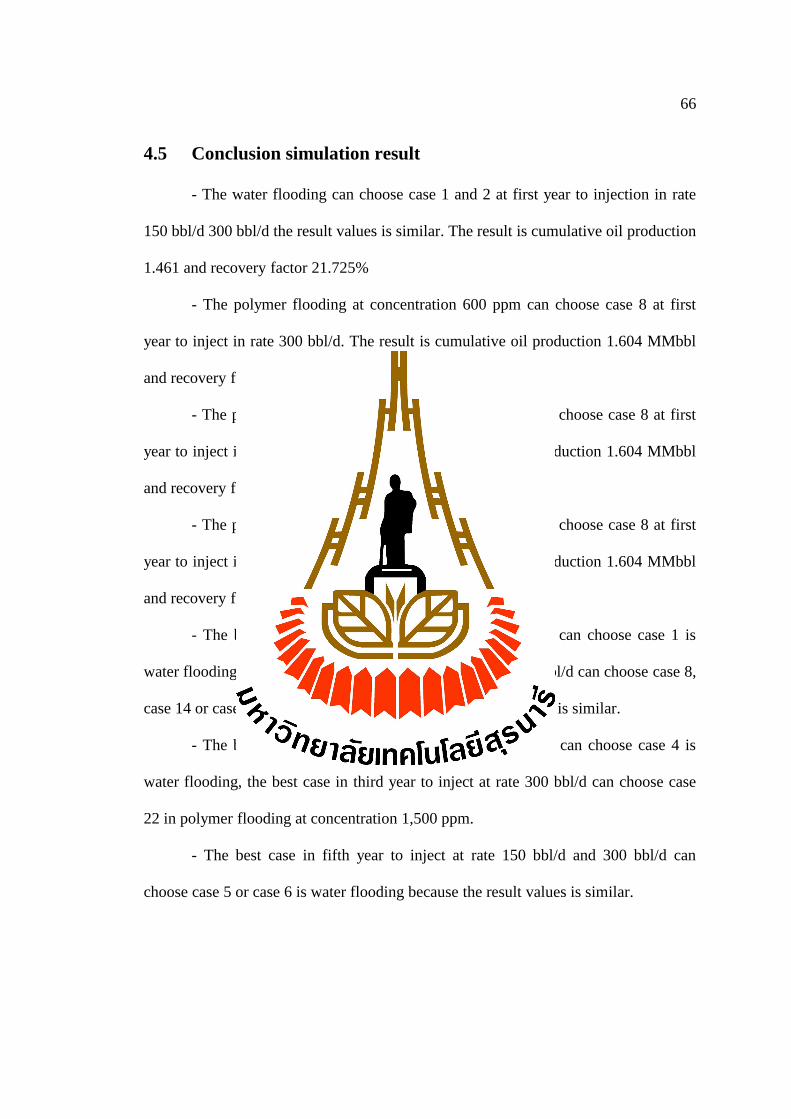
66
4.5 Conclusion simulation result
- The water flooding can choose case 1 and 2 at first year to injection in rate
150 bbl/d 300 bbl/d the result values is similar. The result is cumulative oil production
1.461 and recovery factor 21.725%
- The polymer flooding at concentration 600 ppm can choose case 8 at first
year to inject in rate 300 bbl/d. The result is cumulative oil production 1.604 MMbbl
and recovery factor 26.72%
- The polymer flooding at concentration 1,000 ppm can choose case 8 at first
year to inject in rate 300 bbl/d. The result is cumulative oil production 1.604 MMbbl
and recovery factor 26.72%
- The polymer flooding at concentration 1,500 ppm can choose case 8 at first
year to inject in rate 300 bbl/d. The result is cumulative oil production 1.604 MMbbl
and recovery factor 26.72%
- The best case in first year to inject at rate 150 bbl/d can choose case 1 is
water flooding , the best case in first year to inject at rate 300 bbl/d can choose case 8,
case 14 or case 20 in polymer flooding because the result values is similar.
- The best case in third year to inject at rate 150 bbl/d can choose case 4 is
water flooding, the best case in third year to inject at rate 300 bbl/d can choose case
22 in polymer flooding at concentration 1,500 ppm.
- The best case in fifth year to inject at rate 150 bbl/d and 300 bbl/d can
choose case 5 or case 6 is water flooding because the result values is similar.
67
CHAPTER V
ECONOMIC ANALYSIS
5.1 Objective
This chapter objective is to determine economic parameters that used to
analyze project investment possibility, including on the net present value (NPV),
profit investment ratio (PIR) and internal rate of return (IRR). Compare with all cases
study to find the best case for the Mae Soon oil field.
5.2 Exploration and production schedule
The exploration and production period are following under the Petroleum Acts
“Thailand III” statute are divided into 4 years of exploration period and 20 years of
production period. The work plan of the project can summarize as follows.
1st year: Petroleum concession
2nd year: Geological and geophysical survey
3rd year: Drill exploration well
4th year: Drill development well and prepare to start production plan
5th year: Starting the production plan
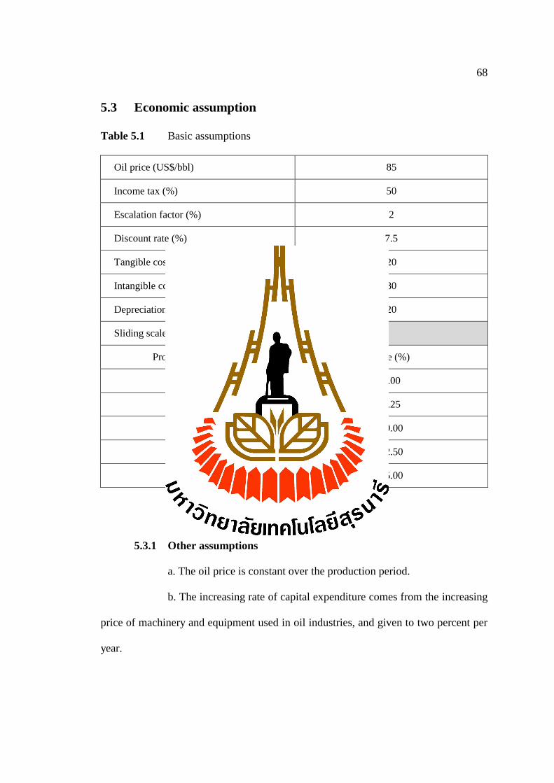
68
5.3 Economic assumption
Table 5.1 Basic assumptions
Oil price (US$/bbl) 85
Income tax (%) 50
Escalation factor (%) 2
Discount rate (%) 7.5
Tangible cost (%) 20
Intangible cost (%) 80
Depreciation of tangible cost (%) 20
Sliding scale royalty
Production level (b/d) Rate (%)
0 - 2,000 5.00
2,000 - 5,000 6.25
5,000 - 10,000 10.00
10,000 - 20,000 12.50
>20,000 15.00
5.3.1 Other assumptions
a. The oil price is constant over the production period.
b. The increasing rate of capital expenditure comes from the increasing
price of machinery and equipment used in oil industries, and given to two percent per
year.
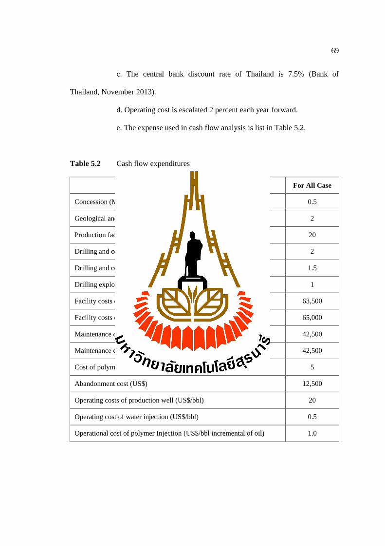
69
c. The central bank discount rate of Thailand is 7.5% (Bank of
Thailand, November 2013).
d. Operating cost is escalated 2 percent each year forward.
e. The expense used in cash flow analysis is list in Table 5.2.
Table 5.2 Cash flow expenditures
Expenditures For All Case
Concession (MMUS$) 0.5
Geological and geophysical survey (MMUS$) 2
Production facility (MMUS$) 20
Drilling and completion production well (MMUS$/well) 2
Drilling and completion injection well (MMUS$/well) 1.5
Drilling exploration & appraisal well (MMUS$) 1
Facility costs of water injection well (US$/well) 63,500
Facility costs of polymer injection well (US$/well) 65,000
Maintenance costs of water injection well (US$/year) 42,500
Maintenance costs of polymer injection well (US$/year) 42,500
Cost of polymer including transportation (US$/kg) 5
Abandonment cost (US$) 12,500
Operating costs of production well (US$/bbl) 20
Operating cost of water injection (US$/bbl) 0.5
Operational cost of polymer Injection (US$/bbl incremental of oil) 1.0
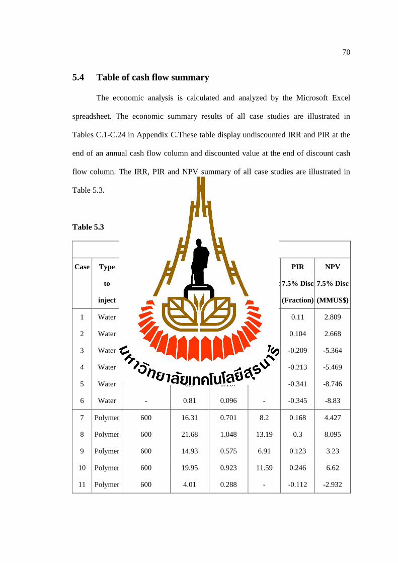
70
5.4 Table of cash flow summary
The economic analysis is calculated and analyzed by the Microsoft Excel
spreadsheet. The economic summary results of all case studies are illustrated in
Tables C.1-C.24 in Appendix C.These table display undiscounted IRR and PIR at the
end of an annual cash flow column and discounted value at the end of discount cash
flow column. The IRR, PIR and NPV summary of all case studies are illustrated in
Table 5.3.
Table 5.3 Cash flow summary of all case studies
Cash flow summary result
Case Type Concentration IRR PIR IRR PIR NPV
to (ppm) Undiscount Undiscount 7.5% Disc 7.5% Disc 7.5% Disc
inject
(%) (Fraction) (%) (Fraction) (MMUS$)
1 Water - 10.7 0.839 2.98 0.11 2.809
2 Water - 10.54 0.825 2.83 0.104 2.668
3 Water - 3.16 0.348 - -0.209 -5.364
4 Water - 3.06 0.336 - -0.213 -5.469
5 Water - 0.9 0.107 - -0.341 -8.746
6 Water - 0.81 0.096 - -0.345 -8.83
7 Polymer 600 16.31 0.701 8.2 0.168 4.427
8 Polymer 600 21.68 1.048 13.19 0.3 8.095
9 Polymer 600 14.93 0.575 6.91 0.123 3.23
10 Polymer 600 19.95 0.923 11.59 0.246 6.62
11 Polymer 600 4.01 0.288 - -0.112 -2.932
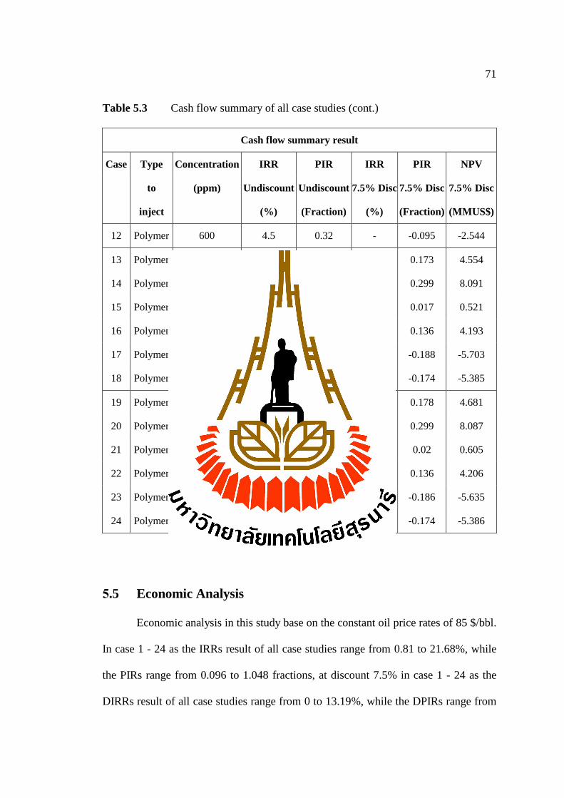
71
Table 5.3 Cash flow summary of all case studies (cont.)
Cash flow summary result
Case Type Concentration IRR PIR IRR PIR NPV
to (ppm) Undiscount Undiscount 7.5% Disc 7.5% Disc 7.5% Disc
inject
(%) (Fraction) (%) (Fraction) (MMUS$)
12 Polymer 600 4.5 0.32 - -0.095 -2.544
13 Polymer 1000 16.52 0.714 8.39 0.173 4.554
14 Polymer 1000 21.68 1.048 13.19 0.299 8.091
15 Polymer 1000 8.36 0.381 0.08 0.017 0.521
16 Polymer 1000 13.39 0.714 5.48 0.136 4.193
17 Polymer 1000 1.77 0.129 - -0.188 -5.703
18 Polymer 1000 2.12 0.151 - -0.174 -5.385
19 Polymer 1500 16.72 0.727 8.58 0.178 4.681
20 Polymer 1500 21.67 1.047 13.18 0.299 8.087
21 Polymer 1500 8.5 0.39 0.93 0.02 0.605
22 Polymer 1500 13.41 0.714 5.5 0.136 4.206
23 Polymer 1500 1.87 0.136 - -0.186 -5.635
24 Polymer 1500 2.11 0.151 - -0.174 -5.386
5.5 Economic Analysis
Economic analysis in this study base on the constant oil price rates of 85 $/bbl.
In case 1 - 24 as the IRRs result of all case studies range from 0.81 to 21.68%, while
the PIRs range from 0.096 to 1.048 fractions, at discount 7.5% in case 1 - 24 as the
DIRRs result of all case studies range from 0 to 13.19%, while the DPIRs range from
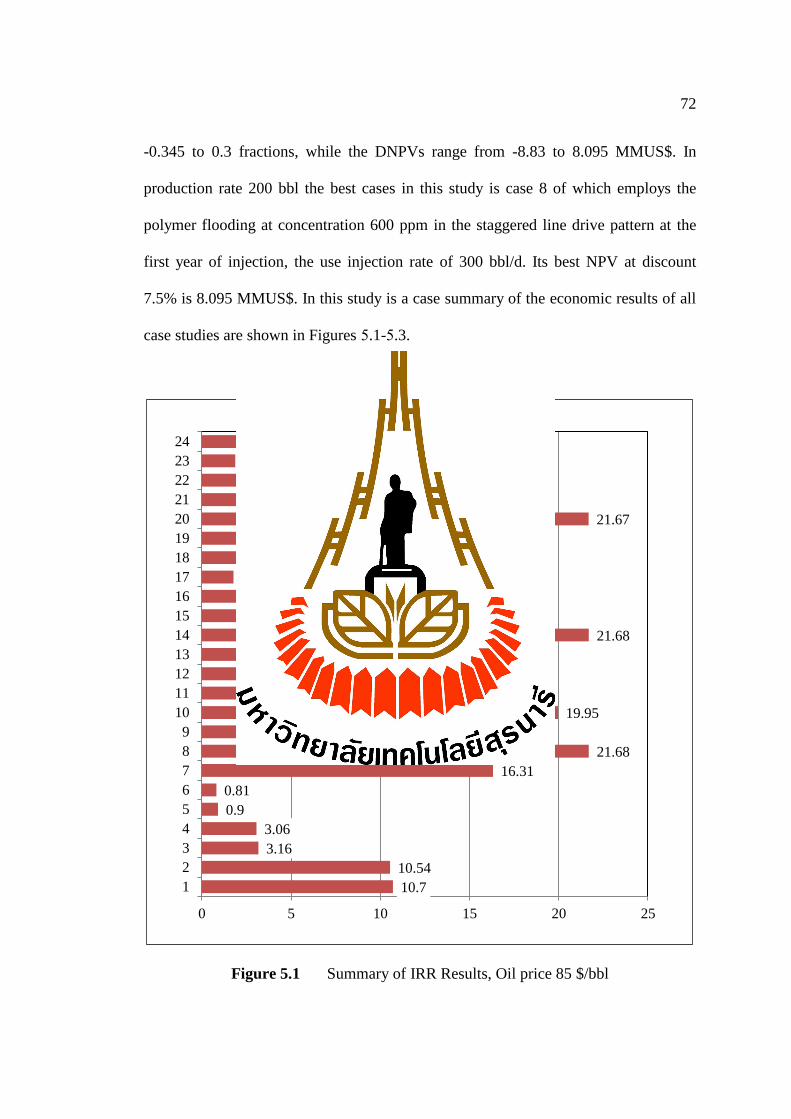
72
-0.345 to 0.3 fractions, while the DNPVs range from -8.83 to 8.095 MMUS$. In
production rate 200 bbl the best cases in this study is case 8 of which employs the
polymer flooding at concentration 600 ppm in the staggered line drive pattern at the
first year of injection, the use injection rate of 300 bbl/d. Its best NPV at discount
7.5% is 8.095 MMUS$. In this study is a case summary of the economic results of all
case studies are shown in Figures 5.1-5.3.
Figure 5.1 Summary of IRR Results, Oil price 85 $/bbl
10.7
10.54
3.16
3.06
0.9
0.81
16.31
21.68
14.93
19.95
4.01
4.5
16.52
21.68
8.36
13.39
1.77
2.12
16.72
21.67
8.5
13.41
1.87
2.11
0 5 10 15 20 25
1
2
3
4
5
6
7
8
9
10
11
12
13
14
15
16
17
18
19
20
21
22
23
24
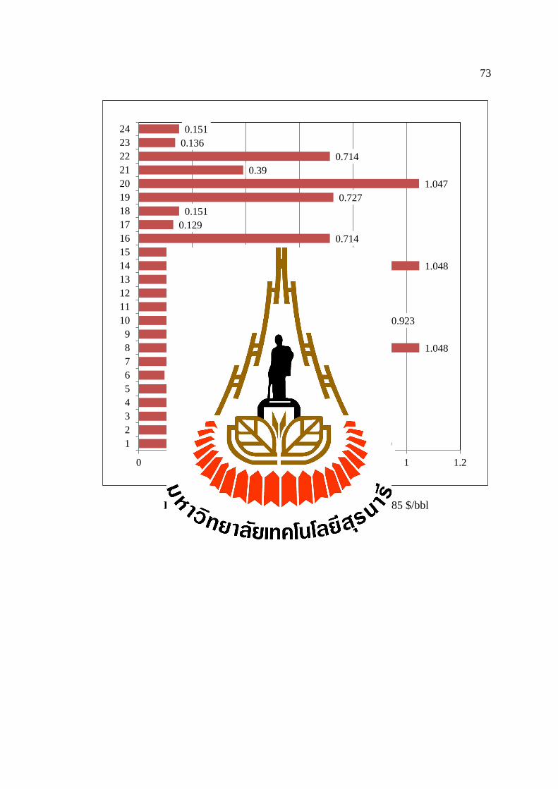
73
Figure 5.2 Summary of PIR Results, Oil price 85 $/bbl
0.839
0.825
0.348
0.336
0.107
0.096
0.701
1.048
0.575
0.923
0.288
0.32
0.714
1.048
0.381
0.714
0.129
0.151
0.727
1.047
0.39
0.714
0.136
0.151
0 0.2 0.4 0.6 0.8 1 1.2
1
2
3
4
5
6
7
8
9
10
11
12
13
14
15
16
17
18
19
20
21
22
23
24
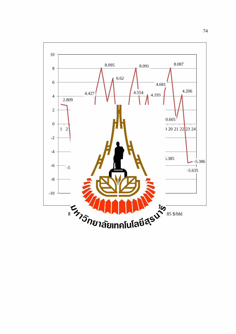
74
Figure 5.3 Summary of NPV Results, Oil price 85 $/bbl
2.809
2.668
-5.364
-5.469
-8.746
-8.83
4.427
8.095
3.23
6.62
-2.932
-2.544
4.554
8.091
0.521
4.193
-5.703
-5.385
4.681
8.087
0.605
4.206
-5.635
-5.386
-10
-8
-6
-4
-2
0
2
4
6
8
10
1 2 3 4 5 6 7 8 9 10 11 12 13 14 15 16 17 18 19 20 21 22 23 24
75
CHAPTER VI
CONCLUSIONS AND DISCUSSIONS
6.1 Introduction
This chapter concludes the research study in term of reservoir model case
study, compare polymer concentration in polymer flooding method and economic
evaluation of water and polymer flooding simulation model for Maesoon oil field in
Fang Basin. Finally, discussion of the research results, problems, and given the
recommendation for future works.
6.2 Conclusions of case study results
This study process of water flooding and polymer flooding, but focuses the
polymer flooding method.
The study focuses on monocline structure style with 6 layers. Used the
reservoir and fluid data from data of Maesoon oil field, but some data are not
available so they are assumed by based on Maesoon data. The porosity ranges from
19 to 29%, and the permeability from about 100 to 230 mD. The study uses reservoir
simulation to evaluate 24 case studies for oil recovery with staggered line drive
patterns. Cases 1 to 24 have the same total production rate of 200 bbl/day at inject rate
150 bbl/d and 300 bbl/d in production life time 20 years, case 1 to 6 in water flooding
at 1st, 3rd and 5th year to inject, case 7 to 12 in polymer flooding at concentration 600
76
ppm, case 13 to 18 in polymer flooding at concentration 1,000 ppm, case 19 to 24 in
polymer flooding at concentration 1,500 ppm. This study used the XCD polymer
(Xanthan gum) is three polymer concentrations.
The result show cases of polymer flooding some case that have high
performance oil recovery efficiency when compared with water flooding, case 1 to 6
show oil recovery from water flooding can best produce 21.725% in case 1 and case
2. Case 7 to 12 show applied polymer flooding, the 1st, 3rd and 5th year of polymer
injection and use polymer concentration at 600 ppm, the best recoveries increased to
26.72% in case 8. Case 13 to 18 show applied polymer flooding, the 1st, 3rd and 5th
year of polymer injection and use polymer concentration at 1,000 ppm, the best
recoveries increased to 26.72% in case 14. Case 19 to 24 show applied polymer
flooding, the 1st, 3rd and 5th year of polymer injection and use polymer concentration
at 1,500 ppm, the best recoveries increased to 26.72% in case 20. In economic
evaluation case 1 to 6 best NPVs is 2.809 MMUS$ in case 1, case 7 to 12 best NPVs
is 8.095 MMUS$ in case 7, case 13 to 18 best NPVs is 8.091 MMUS$, case 19 to 24
best NPVs is 8.087 MMUS$ in case 20. Consider its techniques can choose a case,
polymer concentration 1,500 ppm because increase viscosity in production rates it
best. If consider it economic can choose a case, polymer concentration 600 ppm
because low cost on to inject polymer. But if consider to both result can choose a
case, polymer concentration 1,000 ppm because the result medium in techniques and
economic. Summary of reservoir simulation results is shown in Figure 6.1 and Table
6.1 and shown cash flow summary result in Figure 6.2 and Table 6.2.
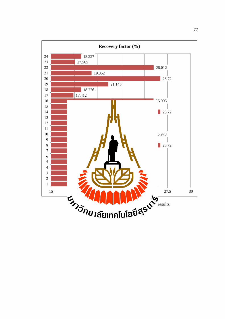
77
Figure 6.1 Summary of reservoir simulation results
21.725
21.725
19.738
19.737
18.427
18.427
20.734
26.72
18.999
25.978
17.259
18.226
20.944
26.72
19.175
25.995
17.412
18.226
21.145
26.72
19.352
26.012
17.565
18.227
15 17.5 20 22.5 25 27.5 30
1
2
3
4
5
6
7
8
9
10
11
12
13
14
15
16
17
18
19
20
21
22
23
24
Recovery factor (%)
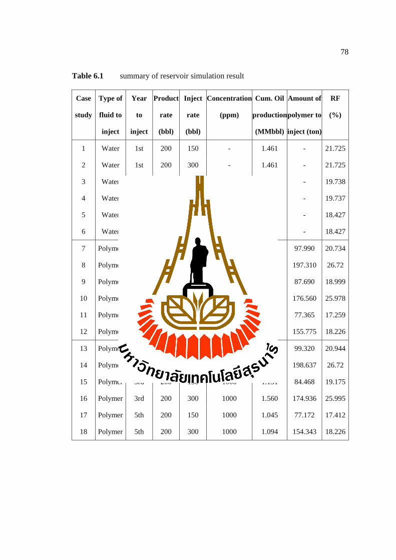
78
Table 6.1 summary of reservoir simulation result
Case Type of Year Product Inject Concentration Cum. Oil Amount of RF
study fluid to to rate rate (ppm) production polymer to (%)
inject inject (bbl) (bbl)
(MMbbl) inject (ton)
1 Water 1st 200 150 - 1.461 - 21.725
2 Water 1st 200 300 - 1.461 - 21.725
3 Water 3rd 200 150 - 1.242 - 19.738
4 Water 3rd 200 300 - 1.242 - 19.737
5 Water 5th 200 150 - 1.096 - 18.427
6 Water 5th 200 300 - 1.096 - 18.427
7 Polymer 1st 200 150 600 1.245 97.990 20.734
8 Polymer 1st 200 300 600 1.604 197.310 26.72
9 Polymer 3rd 200 150 600 1.140 87.690 18.999
10 Polymer 3rd 200 300 600 1.559 176.560 25.978
11 Polymer 5th 200 150 600 1.036 77.365 17.259
12 Polymer 5th 200 300 600 1.093 155.775 18.226
13 Polymer 1st 200 150 1000 1.257 99.320 20.944
14 Polymer 1st 200 300 1000 1.604 198.637 26.72
15 Polymer 3rd 200 150 1000 1.151 84.468 19.175
16 Polymer 3rd 200 300 1000 1.560 174.936 25.995
17 Polymer 5th 200 150 1000 1.045 77.172 17.412
18 Polymer 5th 200 300 1000 1.094 154.343 18.226
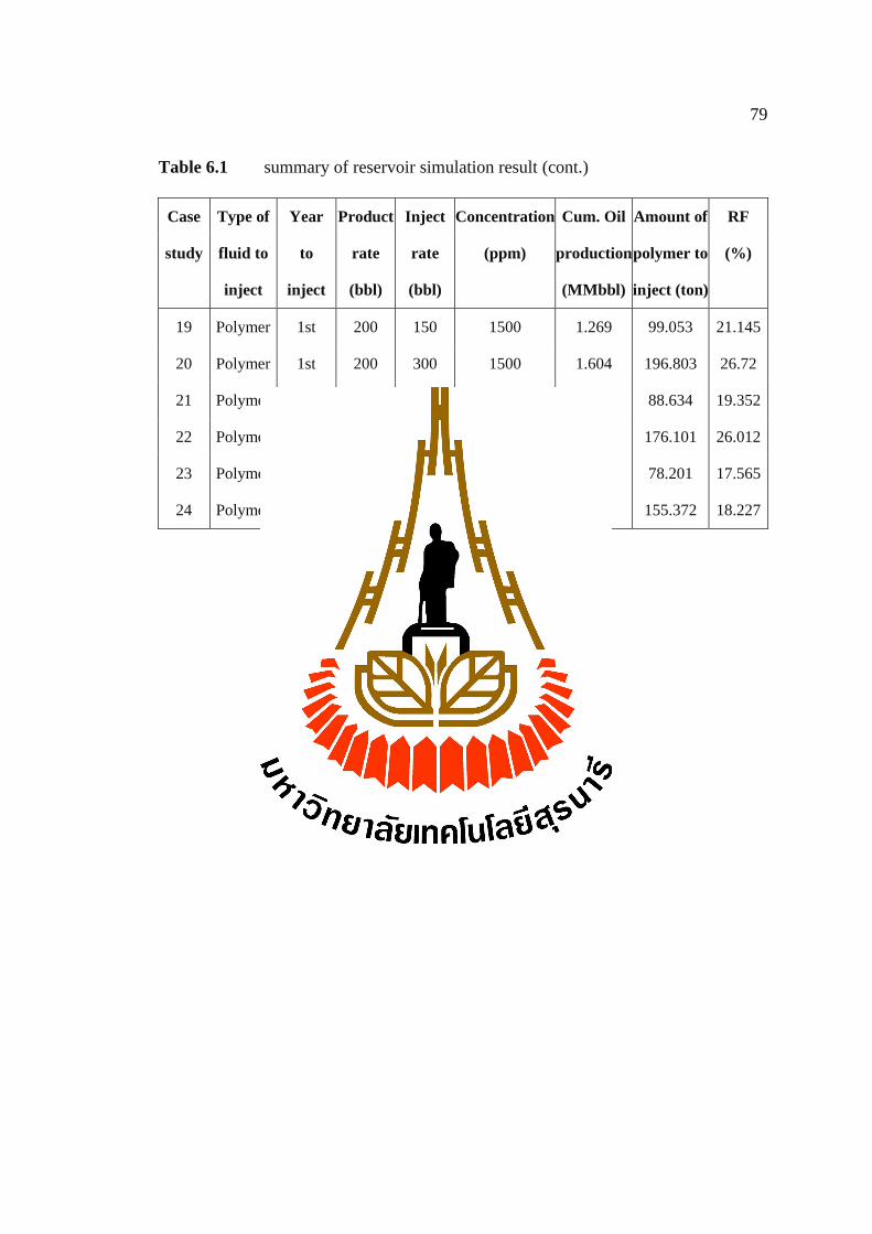
79
Table 6.1 summary of reservoir simulation result (cont.)
Case Type of Year Product Inject Concentration Cum. Oil Amount of RF
study fluid to to rate rate (ppm) production polymer to (%)
inject inject (bbl) (bbl)
(MMbbl) inject (ton)
19 Polymer 1st 200 150 1500 1.269 99.053 21.145
20 Polymer 1st 200 300 1500 1.604 196.803 26.72
21 Polymer 3rd 200 150 1500 1.161 88.634 19.352
22 Polymer 3rd 200 300 1500 1.561 176.101 26.012
23 Polymer 5th 200 150 1500 1.054 78.201 17.565
24 Polymer 5th 200 300 1500 1.093 155.372 18.227
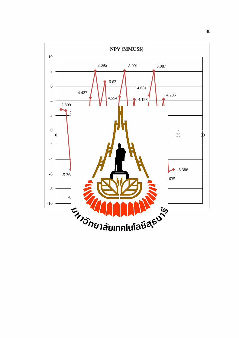
80
Figure 6.2 cash flow summary result
2.809
2.668
-5.364
-5.469
-8.746 -8.83
4.427
8.095
3.23
6.62
-2.932
-2.544
4.554
8.091
0.521
4.193
-5.703
-5.385
4.681
8.087
0.605
4.206
-5.635
-5.386
-10
-8
-6
-4
-2
0
2
4
6
8
10
0 5 10 15 20 25 30
NPV (MMUS$)
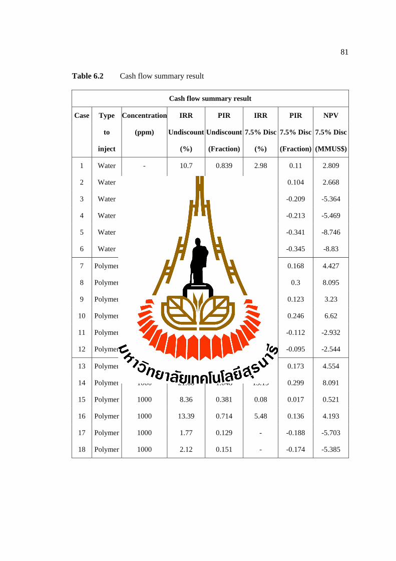
81
Table 6.2 Cash flow summary result
Cash flow summary result
Case Type Concentration IRR PIR IRR PIR NPV
to (ppm) Undiscount Undiscount 7.5% Disc 7.5% Disc 7.5% Disc
inject
(%) (Fraction) (%) (Fraction) (MMUS$)
1 Water - 10.7 0.839 2.98 0.11 2.809
2 Water - 10.54 0.825 2.83 0.104 2.668
3 Water - 3.16 0.348 - -0.209 -5.364
4 Water - 3.06 0.336 - -0.213 -5.469
5 Water - 0.9 0.107 - -0.341 -8.746
6 Water - 0.81 0.096 - -0.345 -8.83
7 Polymer 600 16.31 0.701 8.2 0.168 4.427
8 Polymer 600 21.68 1.048 13.19 0.3 8.095
9 Polymer 600 14.93 0.575 6.91 0.123 3.23
10 Polymer 600 19.95 0.923 11.59 0.246 6.62
11 Polymer 600 4.01 0.288 - -0.112 -2.932
12 Polymer 600 4.5 0.32 - -0.095 -2.544
13 Polymer 1000 16.52 0.714 8.39 0.173 4.554
14 Polymer 1000 21.68 1.048 13.19 0.299 8.091
15 Polymer 1000 8.36 0.381 0.08 0.017 0.521
16 Polymer 1000 13.39 0.714 5.48 0.136 4.193
17 Polymer 1000 1.77 0.129 - -0.188 -5.703
18 Polymer 1000 2.12 0.151 - -0.174 -5.385
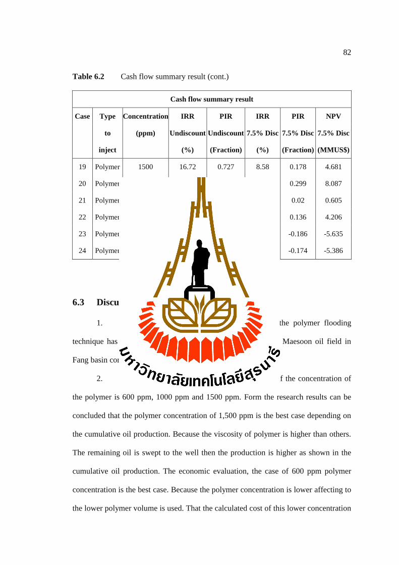
82
Table 6.2 Cash flow summary result (cont.)
Cash flow summary result
Case Type Concentration IRR PIR IRR PIR NPV
to (ppm) Undiscount Undiscount 7.5% Disc 7.5% Disc 7.5% Disc
inject
(%) (Fraction) (%) (Fraction) (MMUS$)
19 Polymer 1500 16.72 0.727 8.58 0.178 4.681
20 Polymer 1500 21.67 1.047 13.18 0.299 8.087
21 Polymer 1500 8.5 0.39 0.93 0.02 0.605
22 Polymer 1500 13.41 0.714 5.5 0.136 4.206
23 Polymer 1500 1.87 0.136 - -0.186 -5.635
24 Polymer 1500 2.11 0.151 - -0.174 -5.386
6.3 Discussions
1. The reservoir simulation result indicates that the polymer flooding
technique has the most potential in increasing oil recovery of Maesoon oil field in
Fang basin compared to the water flooding techniques
2. In polymer flooding method, change the value of the concentration of
the polymer is 600 ppm, 1000 ppm and 1500 ppm. Form the research results can be
concluded that the polymer concentration of 1,500 ppm is the best case depending on
the cumulative oil production. Because the viscosity of polymer is higher than others.
The remaining oil is swept to the well then the production is higher as shown in the
cumulative oil production. The economic evaluation, the case of 600 ppm polymer
concentration is the best case. Because the polymer concentration is lower affecting to
the lower polymer volume is used. That the calculated cost of this lower concentration
83
case is cheaper than others. Both the cumulative oil production and economic
evaluations are contrasted and hard for consideration. However, the case of 1,000
ppm polymer concentration is proper. Due to it is still high in recovery factor and
production rate moreover, it is 2nd best case of both evaluations.
3. The best case of this study is case use injection rate 150 bbl are
choosing polymer flooding at concentration 1,500 ppm. During the first year to inject,
at the oil price rate 85$/bbl, the NPVs is 4.681 MMUS$. The best case use injection
rate 300 bbl are choosing polymer flooding at concentration 600 ppm. During the first
year to inject, the NPVs is 8.095 MMUS$. Why the choose polymer flooding at
concentration 600 ppm because the rate in polymer inject is low compared to the each
case in polymer flooding for decrease cost inject polymer.
4. In all cases, in the fifth year of injection, in water and polymer
flooding are should choose not to do because to be produced, but not worth the cost to
do. In water flooding at third year to inject should not to do. Polymer flooding is the
best techniques in improving efficiency of oil recovery and economic values. But in
the real field operation, it is unlikely that the operation can take place in the first year
because water and polymer flooding projects require at least 3 to 5 years in collecting
data of reservoir properties and history of production rates.
5. History matching should be compared to the real field and the reservoir
simulation because it is crucial in producing more accurate results. The study also
finds that the more reservoir properties data obtained, the more accurate the results
are. However, production rates are not included in this study due to the inaccessibility
6. Reliability of simulation result depends on confidential of rock and
fluid properties data collected from the oil field.

84
7. For future study, the locations of production and injection wells can be
changed to five spot, seven spot, and nine spot, and peripheral flood patterns in order
to find oil recovery efficiency and economic values in Maesoon oil field. It is
suggested that the researchers should have sufficient understanding of program
application (ECLIPSE and Surfer) in order to input data into the simulations and
produce highly accurate results.
85
References
Berger, B. D. and Anderson, K. E. (1992). Modern Petroleum: A Basic Primer of
the Industry. 3rd
ed. Tulsa, Oklahoma: PennWell Books.
Bradley, H. B. and Gipson, F. W. (1987). Petroleum Engineering Handbook.
Richardson, TX, U.S.A.: Society of Petroleum Engineers.
Bybee, K. (2007). Reduced Well Spacing Combined with Polymer Flooding Improves
Oil Recovery from Marginal Reservoirs. Journal of Petroleum Technology.
59(01).
Defense Energy Department, Exploration and Production Division (2004). Drilling.
Faisal, S. A., Badr, A. A., Sami, M. A., John, N. M. V. W., Henri, F. J.,Said, A. H.,
Khalfan, S., Kumar, P. C., and Ravula, C. (2012). Polymer Flooding in a
Large Field in Soult Oman - Initial Results and Future Plan. Journal of
Petroleum Technology. 65(01): 4 pp.
Gerding, M. (1986). Fundamental of Petroleum. Texas: Petroleum Extension
Service.
Green, D. W. and Willhite, G. P. (1998). Enhanced Oil Recovery. Richardson, TX:
Society of Petroleum Engineers.
Kanarak, J. (2011). Enhanced Oil Recovery with Polymer Flooding for Oil Field
in Phitsanulok Basin. Master Thesis, Suranaree University of Technology,
Thailand.
86
Maheshwari, Y. K. (2011). A Comparative Simulation Study of Chemical EOR
Methodologies (Alkaline, Surfactant and/or Polymer) Applied to
Nornefield E-Segment. Master Thesis, Department of Petroleum Engineering
and Applied Geophysics, Norwegian University of Science and Technology,
Norway.
Nicholls, C. A., Boom, W., Geel, J., Khodori, A. S., and Lawati, A. M. (2000).
Fracture Modeling as a Key to Waterflood Development. 52. 42-43.
Noianusontigul, K (2008). Numerical Simulation by ECLIPSE on Polymer
Injection in the Benchamas Oilfield as an EOR Method Using the High-
Performance Computing Cluster. Master Thesis, Asian Institute of
Technology, Thailand.
Nuntajun, R. (2009). Seismic Stratigraphy of the Fang Basin, Chiang Mai,
Thiland. Chiang Mai, Thailand: Department of Geological Sciences, Chiang
Mai University.
Schlumberger (2003). ECLIPSE Technical Description. Reservoir Simulation
Software. Licensed and Supported by GeoQuest.
Schlumberger Oilfield glossary (2009). XRD & XRF. [On-line]. Available:
http://www.glossary.oilfield.slb.com/search.cfm
Settakul, N. (2009). Fang Oilfield Development. Walailak Journal of Science and
Tehnology. 6(1): 1-15.
Supaprom, C. (2012). A Comparison Study of Five-Spot and Nine-Spot Water
Injection Patterns to Enhance Oil Recovery of Maesoon Oil Field by
Computer Simulation. Master Thesis, Suranaree University of Technology,

87
Thailand.
Thang, P. D. (2005). Enhanced Oil Recovery in Basement Rock of the White
Tiger field in offshore Southern Vietnam. Master Thesis, Asian Institute of
Technology, Thailand.
Thongsumrit, T. (2012). Comparison of the Oil Recovery between Water Flooding
and Polymer Flooding for Suphan buri basin. Master Thesis, Suranaree
University of Technology, Thailand.
Willhite, G. P. (2003). Waterflooding. Richardson, TX: Society of Petroleum
Engineers.
Wongsirasawad, L. (2002). 20 Successful Years of Sirikit Oilfield. Thailand
Petroleum Conference 2002, Bangkok: Thailand.

APPENDIX A
SIMULATION DATA
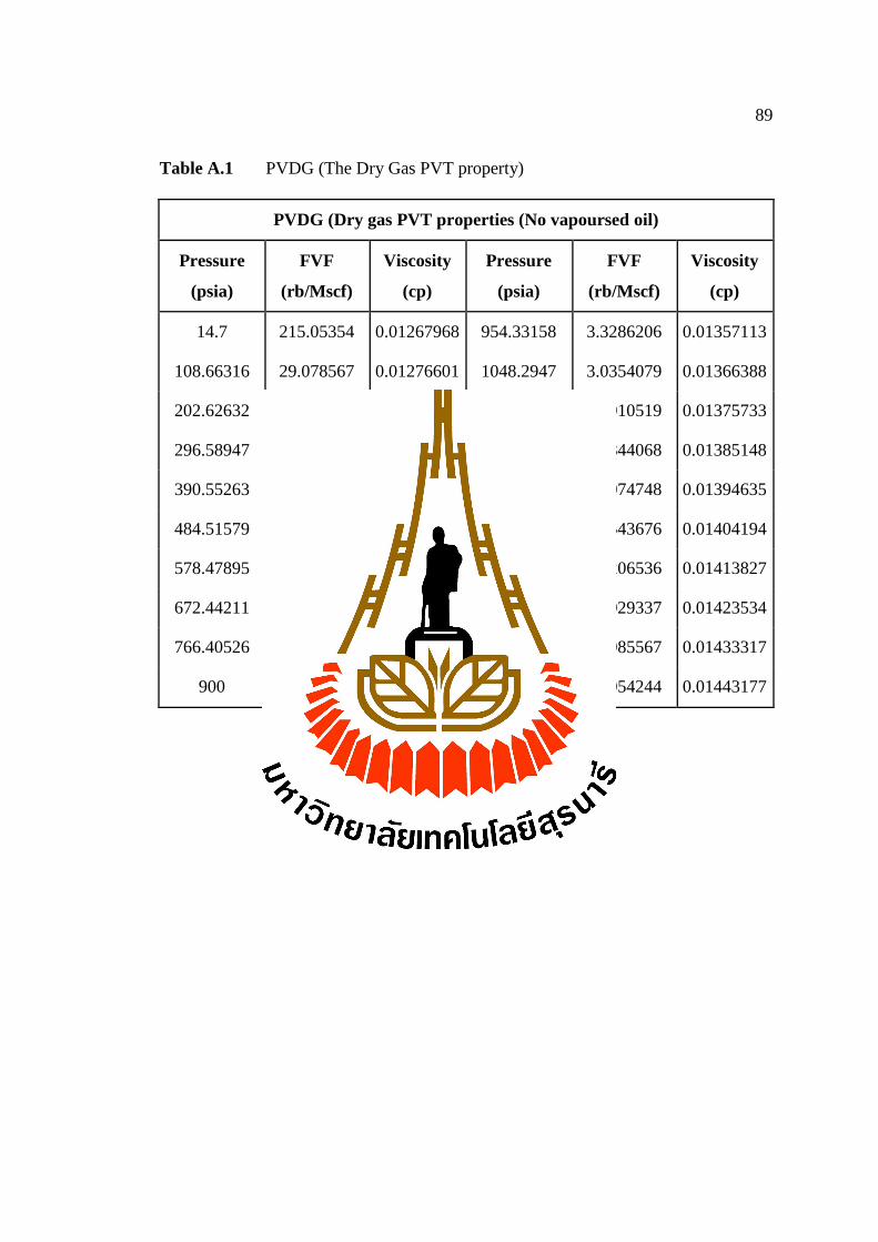
89
Table A.1 PVDG (The Dry Gas PVT property)
PVDG (Dry gas PVT properties (No vapoursed oil)
Pressure
(psia)
FVF
(rb/Mscf)
Viscosity
(cp)
Pressure
(psia)
FVF
(rb/Mscf)
Viscosity
(cp)
14.7 215.05354 0.01267968 954.33158 3.3286206 0.01357113
108.66316 29.078567 0.01276601 1048.2947 3.0354079 0.01366388
202.62632 15.589737 0.01285294 1142.2579 2.7910519 0.01375733
296.58947 10.649988 0.01294048 1236.2211 2.5844068 0.01385148
390.55263 8.0888839 0.01302865 1330.1842 2.4074748 0.01394635
484.51579 6.5225623 0.01311744 1424.1474 2.2543676 0.01404194
578.47895 5.4662877 0.01320686 1518.1105 2.1206536 0.01413827
672.44211 4.7062572 0.01329694 1612.0737 2.0029337 0.01423534
766.40526 4.1335156 0.01338767 1706.0368 1.8985567 0.01433317
900 3.5264576 0.01351781 1800 1.8054244 0.01443177
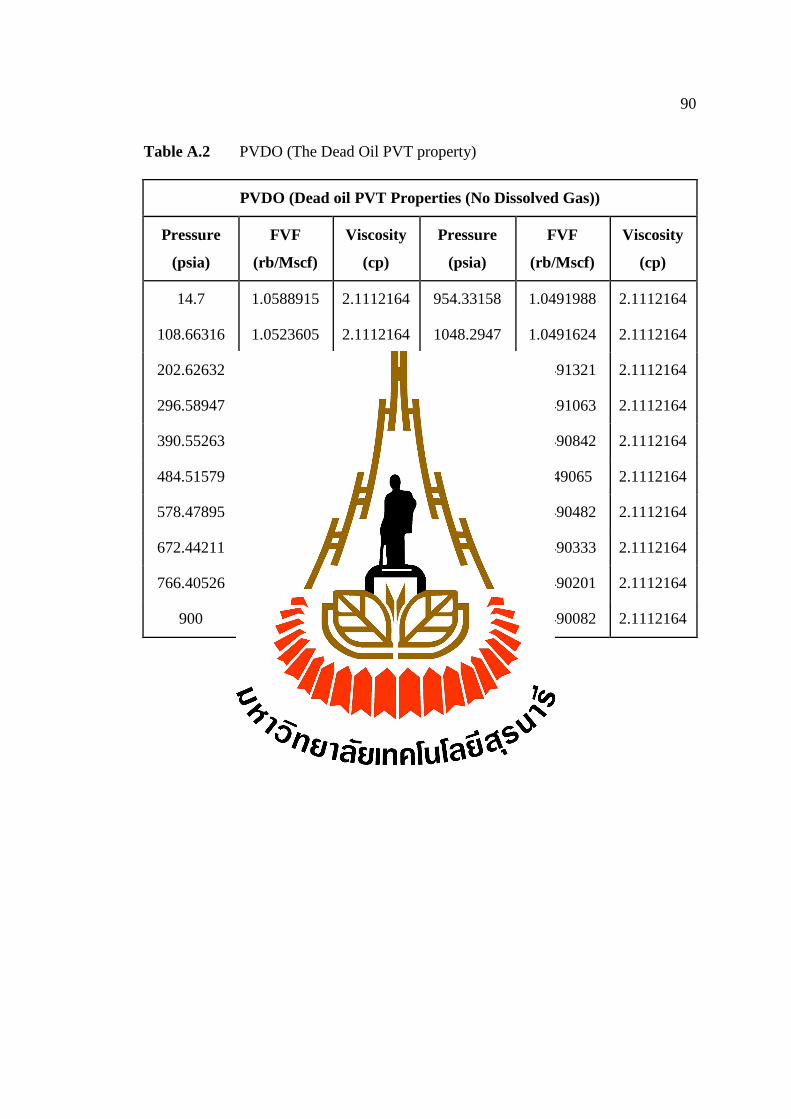
90
Table A.2 PVDO (The Dead Oil PVT property)
PVDO (Dead oil PVT Properties (No Dissolved Gas))
Pressure
(psia)
FVF
(rb/Mscf)
Viscosity
(cp)
Pressure
(psia)
FVF
(rb/Mscf)
Viscosity
(cp)
14.7 1.0588915 2.1112164 954.33158 1.0491988 2.1112164
108.66316 1.0523605 2.1112164 1048.2947 1.0491624 2.1112164
202.62632 1.0507048 2.1112164 1142.2579 1.0491321 2.1112164
296.58947 1.0500988 2.1112164 1236.2211 1.0491063 2.1112164
390.55263 1.0497845 2.1112164 1330.1842 1.0490842 2.1112164
484.51579 1.0495922 2.1112164 1424.1474 1.049065 2.1112164
578.47895 1.0494624 2.1112164 1518.1105 1.0490482 2.1112164
672.44211 1.0493689 2.1112164 1612.0737 1.0490333 2.1112164
766.40526 1.0492983 2.1112164 1706.0368 1.0490201 2.1112164
900 1.0492233 2.1112164 1800 1.0490082 2.1112164

APPENDIX B
POLYMER DATA
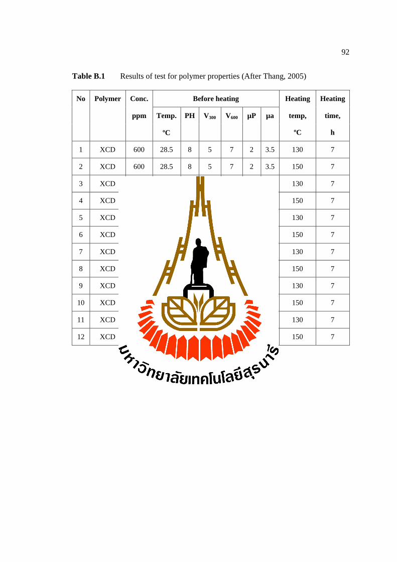
92
Table B.1 Results of test for polymer properties (After Thang, 2005)
No Polymer Conc. Before heating Heating Heating
ppm Temp. PH V300 V600 µP µa temp,
ºC
time,
h ºC
1 XCD 600 28.5 8 5 7 2 3.5 130 7
2 XCD 600 28.5 8 5 7 2 3.5 150 7
3 XCD 1200 28.5 8 7 9 2 4.5 130 7
4 XCD 1200 28.5 8 7 9 2 4.5 150 7
5 XCD 1800 30.0 8 8 12 4 6 130 7
6 XCD 1800 30.0 8 8 12 4 6 150 7
7 XCD 2400 30.5 8 10 14 4 7 130 7
8 XCD 2400 30.5 8 10 14 4 7 150 7
9 XCD 3000 30.5 8 12 17 5 8.5 130 7
10 XCD 3000 30.5 8 12 17 5 8.5 150 7
11 XCD 3000 26.0 8 15 20 5 9.8 130 7
12 XCD 3000 26.0 8 15 20 5 9.8 150 7
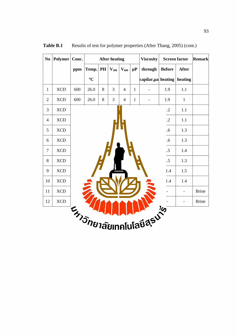
93
Table B.1 Results of test for polymer properties (After Thang, 2005) (cont.)
No Polymer Conc. After heating Viscosity Screen factor Remark
ppm Temp. PH V300 V600 µP through Before After
ºC capilar,µa heating heating
1 XCD 600 26.0 8 3 4 1 - 1.9 1.1
2 XCD 600 26.0 8 3 4 1 - 1.9 1
3 XCD 1200 28.0 8 3 4.5 1.5 - 2.2 1.1
4 XCD 1200 30.0 8 3 4.5 1.5 - 2.2 1.1
5 XCD 1800 30.0 8 4 6 2 1.0 2.6 1.3
6 XCD 1800 30.0 8 3 4.5 1.5 1.0 2.6 1.3
7 XCD 2400 30.5 8 4 6 2 1.1 4.5 1.4
8 XCD 2400 30.5 8 3 5 2 1.0 4.5 1.3
9 XCD 3000 30.5 8 5 7 2 1.7 11.4 1.5
10 XCD 3000 30.5 8 3 5 2 1.4 11.4 1.4
11 XCD 3000 26.0 8 4 6 2 - - - Brine
12 XCD 3000 26.0 8 3.5 5.5 2 - - - Brine

APPENDIX C
CASH FLOW SUMMARY
95
C.1 Cash flow summary result table
The economic analysis is calculated and analyzed by using Microsoft Excels
spreadsheet. The economic summary results of all case studies are illustrated in
Tables C.1 - C.24. In Tables C.1 - C.24 display undiscounted IRR and PIR at the end
of annual cash flow column and discounted value at the end of discount cash flow
column. The IRR, PIR and NPV summary of all case studies are illustrated in Table
C.25.

96
Table C.1 Cash flow summary of case 1
Year
Cash flow summary Discount cash
flow
Oil
production
total
Gross
revenue CAPEX OPEX
Government take Annual
cash flow Royalty Inc. tax
(bbl/year) (MMUS$) (MMUS$) (MMUS$) (MMUS$) (MMUS$) (MMUS$) (MMUS$)
1 0.000 0.000 0.500 0.000 0.000 0.000 -0.500 -0.465
2 0.000 0.000 2.000 0.000 0.000 0.000 -2.000 -1.731
3 0.000 0.000 1.000 0.000 0.000 0.000 -1.000 -0.805
4 0.000 0.000 22.131 0.000 0.000 0.000 -5.706 -4.273
5 73,200 6.222 0.000 1.660 0.311 0.000 0.144 0.101
6 73,000 6.205 0.000 1.689 0.310 0.050 0.050 0.032
7 73,000 6.205 0.000 1.723 0.310 0.033 0.033 0.020
8 73,000 6.205 0.000 1.757 0.310 0.016 0.016 0.009
9 73,200 6.222 0.000 1.797 0.311 2.057 2.057 1.073
10 73,000 6.205 0.000 1.828 0.310 2.033 2.033 0.986
11 73,000 6.205 0.000 1.865 0.310 2.015 2.015 0.909
12 73,000 6.205 0.000 1.902 0.310 1.996 1.996 0.838
13 73,200 6.222 0.000 1.945 0.311 1.983 1.983 0.774
14 73,000 6.205 0.000 1.979 0.310 1.958 1.958 0.711
15 73,000 6.205 0.000 2.019 0.310 1.938 1.938 0.655
16 73,000 6.205 0.000 2.059 0.310 1.918 1.918 0.603
17 73,200 6.222 0.000 2.106 0.311 1.903 1.903 0.556
18 73,000 6.205 0.000 2.142 0.310 1.876 1.876 0.510
19 73,000 6.205 0.000 2.185 0.310 1.855 1.855 0.469
20 73,000 6.205 0.000 2.229 0.310 1.833 1.833 0.432
21 73,200 6.222 0.000 2.279 0.311 1.816 1.816 0.398
22 73,000 6.205 0.000 2.319 0.310 1.788 1.788 0.364
23 73,000 6.205 0.000 2.365 0.310 1.765 1.765 0.334
24 73,000 6.205 0.000 2.412 0.310 1.741 1.741 0.307
Total 1,461,000 124.185 25.631 40.262 6.209 30.572 21.511 2.809
IRR 10.70% 2.98%
PIR 0.839 0.110

97
Table C.2 Cash flow summary of case 2
Year
Cash flow summary Discount cash
flow
Oil
production
total
Gross
revenue CAPEX OPEX
Government take Annual
cash flow Royalty Inc. tax
(bbl/year) (MMUS$) (MMUS$) (MMUS$) (MMUS$) (MMUS$) (MMUS$) (MMUS$)
1 0.000 0.000 0.500 0.000 0.000 0.000 -0.500 -0.465
2 0.000 0.000 2.000 0.000 0.000 0.000 -2.000 -1.731
3 0.000 0.000 1.000 0.000 0.000 0.000 -1.000 -0.805
4 0.000 0.000 22.131 0.000 0.000 0.000 -5.706 -4.273
5 73,200 6.222 0.000 1.690 0.311 0.000 0.115 0.080
6 73,000 6.205 0.000 1.719 0.310 0.035 0.035 0.022
7 73,000 6.205 0.000 1.754 0.310 0.017 0.017 0.011
8 73,000 6.205 0.000 1.789 0.310 0.000 0.000 0.000
9 73,200 6.222 0.000 1.829 0.311 2.041 2.041 1.064
10 73,000 6.205 0.000 1.861 0.310 2.017 2.017 0.979
11 73,000 6.205 0.000 1.898 0.310 1.998 1.998 0.902
12 73,000 6.205 0.000 1.936 0.310 1.979 1.979 0.831
13 73,200 6.222 0.000 1.980 0.311 1.965 1.965 0.768
14 73,000 6.205 0.000 2.014 0.310 1.940 1.940 0.705
15 73,000 6.205 0.000 2.055 0.310 1.920 1.920 0.649
16 73,000 6.205 0.000 2.096 0.310 1.899 1.899 0.597
17 73,200 6.222 0.000 2.143 0.311 1.884 1.884 0.551
18 73,000 6.205 0.000 2.181 0.310 1.857 1.857 0.505
19 73,000 6.205 0.000 2.224 0.310 1.835 1.835 0.464
20 73,000 6.205 0.000 2.269 0.310 1.813 1.813 0.427
21 73,200 6.222 0.000 2.320 0.311 1.795 1.795 0.393
22 73,000 6.205 0.000 2.360 0.310 1.767 1.767 0.360
23 73,000 6.205 0.000 2.407 0.310 1.744 1.744 0.330
24 73,000 6.205 0.000 2.456 0.310 1.720 1.720 0.303
Total 1,461,000 124.185 25.631 40.983 6.209 30.227 21.135 2.668
IRR 10.54% 2.83%
PIR 0.825 0.104

98
Table C.3 Cash flow summary of case 3
Year
Cash flow summary Discount cash
flow
Oil
production
total
Gross
revenue CAPEX OPEX
Government take Annual
cash flow Royalty Inc. tax
(bbl/year) (MMUS$) (MMUS$) (MMUS$) (MMUS$) (MMUS$) (MMUS$) (MMUS$)
1 0.000 0.000 0.500 0.000 0.000 0.000 -0.500 -0.465
2 0.000 0.000 2.000 0.000 0.000 0.000 -2.000 -1.731
3 0.000 0.000 1.000 0.000 0.000 0.000 -1.000 -0.805
4 0.000 0.000 22.131 0.000 0.000 0.000 -5.706 -4.273
5 0 0.000 0.000 0.000 0.000 0.000 -4.106 -2.860
6 0 0.000 0.000 0.000 0.000 0.000 -4.106 -2.661
7 200 0.017 0.000 0.052 0.001 0.000 -4.142 -2.497
8 72,800 6.188 0.000 1.753 0.309 0.010 0.010 0.006
9 73,200 6.222 0.000 1.797 0.311 2.057 2.057 1.073
10 73,000 6.205 0.000 1.828 0.310 2.033 2.033 0.986
11 73,000 6.205 0.000 1.865 0.310 2.015 2.015 0.909
12 73,000 6.205 0.000 1.902 0.310 1.996 1.996 0.838
13 73,200 6.222 0.000 1.945 0.311 1.983 1.983 0.774
14 73,000 6.205 0.000 1.979 0.310 1.958 1.958 0.711
15 73,000 6.205 0.000 2.019 0.310 1.938 1.938 0.655
16 73,000 6.205 0.000 2.059 0.310 1.918 1.918 0.603
17 73,200 6.222 0.000 2.106 0.311 1.903 1.903 0.556
18 73,000 6.205 0.000 2.142 0.310 1.876 1.876 0.510
19 73,000 6.205 0.000 2.185 0.310 1.855 1.855 0.469
20 73,000 6.205 0.000 2.229 0.310 1.833 1.833 0.432
21 73,200 6.222 0.000 2.279 0.311 1.816 1.816 0.398
22 73,000 6.205 0.000 2.319 0.310 1.788 1.788 0.364
23 73,000 6.205 0.000 2.365 0.310 1.765 1.765 0.334
24 73,000 6.205 0.000 2.412 0.310 1.741 1.741 0.307
Total 1,241,800 105.553 25.631 35.237 5.278 30.484 8.923 -5.364
IRR 3.16% -
PIR 0.348 -0.209
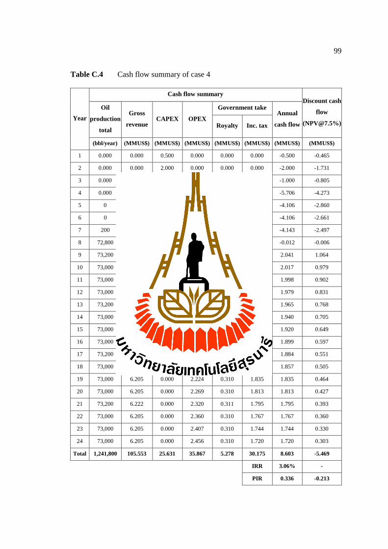
99
Table C.4 Cash flow summary of case 4
Year
Cash flow summary Discount cash
flow
Oil
production
total
Gross
revenue CAPEX OPEX
Government take Annual
cash flow Royalty Inc. tax
(bbl/year) (MMUS$) (MMUS$) (MMUS$) (MMUS$) (MMUS$) (MMUS$) (MMUS$)
1 0.000 0.000 0.500 0.000 0.000 0.000 -0.500 -0.465
2 0.000 0.000 2.000 0.000 0.000 0.000 -2.000 -1.731
3 0.000 0.000 1.000 0.000 0.000 0.000 -1.000 -0.805
4 0.000 0.000 22.131 0.000 0.000 0.000 -5.706 -4.273
5 0 0.000 0.000 0.000 0.000 0.000 -4.106 -2.860
6 0 0.000 0.000 0.000 0.000 0.000 -4.106 -2.661
7 200 0.017 0.000 0.053 0.001 0.000 -4.143 -2.497
8 72,800 6.188 0.000 1.784 0.309 0.000 -0.012 -0.006
9 73,200 6.222 0.000 1.829 0.311 2.041 2.041 1.064
10 73,000 6.205 0.000 1.861 0.310 2.017 2.017 0.979
11 73,000 6.205 0.000 1.898 0.310 1.998 1.998 0.902
12 73,000 6.205 0.000 1.936 0.310 1.979 1.979 0.831
13 73,200 6.222 0.000 1.980 0.311 1.965 1.965 0.768
14 73,000 6.205 0.000 2.014 0.310 1.940 1.940 0.705
15 73,000 6.205 0.000 2.055 0.310 1.920 1.920 0.649
16 73,000 6.205 0.000 2.096 0.310 1.899 1.899 0.597
17 73,200 6.222 0.000 2.143 0.311 1.884 1.884 0.551
18 73,000 6.205 0.000 2.181 0.310 1.857 1.857 0.505
19 73,000 6.205 0.000 2.224 0.310 1.835 1.835 0.464
20 73,000 6.205 0.000 2.269 0.310 1.813 1.813 0.427
21 73,200 6.222 0.000 2.320 0.311 1.795 1.795 0.393
22 73,000 6.205 0.000 2.360 0.310 1.767 1.767 0.360
23 73,000 6.205 0.000 2.407 0.310 1.744 1.744 0.330
24 73,000 6.205 0.000 2.456 0.310 1.720 1.720 0.303
Total 1,241,800 105.553 25.631 35.867 5.278 30.175 8.603 -5.469
IRR 3.06% -
PIR 0.336 -0.213
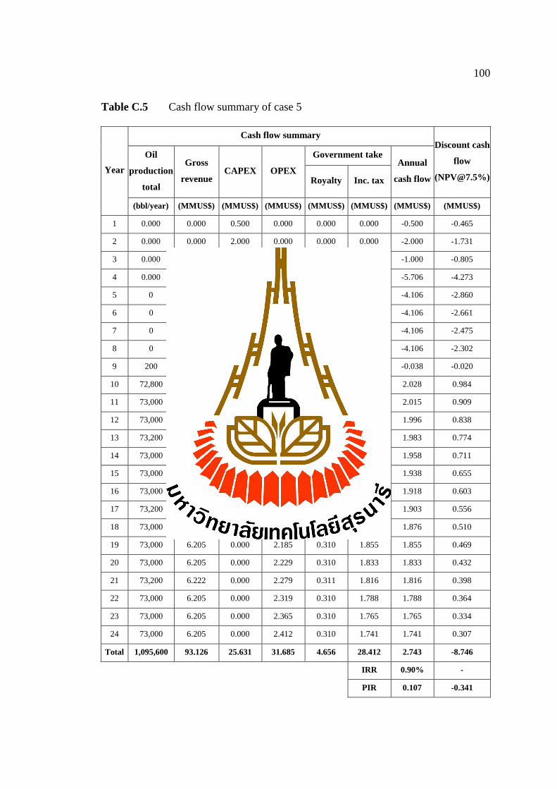
100
Table C.5 Cash flow summary of case 5
Year
Cash flow summary Discount cash
flow
Oil
production
total
Gross
revenue CAPEX OPEX
Government take Annual
cash flow Royalty Inc. tax
(bbl/year) (MMUS$) (MMUS$) (MMUS$) (MMUS$) (MMUS$) (MMUS$) (MMUS$)
1 0.000 0.000 0.500 0.000 0.000 0.000 -0.500 -0.465
2 0.000 0.000 2.000 0.000 0.000 0.000 -2.000 -1.731
3 0.000 0.000 1.000 0.000 0.000 0.000 -1.000 -0.805
4 0.000 0.000 22.131 0.000 0.000 0.000 -5.706 -4.273
5 0 0.000 0.000 0.000 0.000 0.000 -4.106 -2.860
6 0 0.000 0.000 0.000 0.000 0.000 -4.106 -2.661
7 0 0.000 0.000 0.000 0.000 0.000 -4.106 -2.475
8 0 0.000 0.000 0.000 0.000 0.000 -4.106 -2.302
9 200 0.017 0.000 0.055 0.001 0.000 -0.038 -0.020
10 72,800 6.188 0.000 1.823 0.309 2.028 2.028 0.984
11 73,000 6.205 0.000 1.865 0.310 2.015 2.015 0.909
12 73,000 6.205 0.000 1.902 0.310 1.996 1.996 0.838
13 73,200 6.222 0.000 1.945 0.311 1.983 1.983 0.774
14 73,000 6.205 0.000 1.979 0.310 1.958 1.958 0.711
15 73,000 6.205 0.000 2.019 0.310 1.938 1.938 0.655
16 73,000 6.205 0.000 2.059 0.310 1.918 1.918 0.603
17 73,200 6.222 0.000 2.106 0.311 1.903 1.903 0.556
18 73,000 6.205 0.000 2.142 0.310 1.876 1.876 0.510
19 73,000 6.205 0.000 2.185 0.310 1.855 1.855 0.469
20 73,000 6.205 0.000 2.229 0.310 1.833 1.833 0.432
21 73,200 6.222 0.000 2.279 0.311 1.816 1.816 0.398
22 73,000 6.205 0.000 2.319 0.310 1.788 1.788 0.364
23 73,000 6.205 0.000 2.365 0.310 1.765 1.765 0.334
24 73,000 6.205 0.000 2.412 0.310 1.741 1.741 0.307
Total 1,095,600 93.126 25.631 31.685 4.656 28.412 2.743 -8.746
IRR 0.90% -
PIR 0.107 -0.341

101
Table C.6 Cash flow summary of case 6
Year
Cash flow summary Discount cash
flow
Oil
production
total
Gross
revenue CAPEX OPEX
Government take Annual
cash flow Royalty Inc. tax
(bbl/year) (MMUS$) (MMUS$) (MMUS$) (MMUS$) (MMUS$) (MMUS$) (MMUS$)
1 0.000 0.000 0.500 0.000 0.000 0.000 -0.500 -0.465
2 0.000 0.000 2.000 0.000 0.000 0.000 -2.000 -1.731
3 0.000 0.000 1.000 0.000 0.000 0.000 -1.000 -0.805
4 0.000 0.000 22.131 0.000 0.000 0.000 -5.706 -4.273
5 0 0.000 0.000 0.000 0.000 0.000 -4.106 -2.860
6 0 0.000 0.000 0.000 0.000 0.000 -4.106 -2.661
7 0 0.000 0.000 0.000 0.000 0.000 -4.106 -2.475
8 0 0.000 0.000 0.000 0.000 0.000 -4.106 -2.302
9 200 0.017 0.000 0.055 0.001 0.000 -0.039 -0.020
10 72,800 6.188 0.000 1.856 0.309 2.011 2.011 0.976
11 73,000 6.205 0.000 1.898 0.310 1.998 1.998 0.902
12 73,000 6.205 0.000 1.936 0.310 1.979 1.979 0.831
13 73,200 6.222 0.000 1.980 0.311 1.965 1.965 0.768
14 73,000 6.205 0.000 2.014 0.310 1.940 1.940 0.705
15 73,000 6.205 0.000 2.055 0.310 1.920 1.920 0.649
16 73,000 6.205 0.000 2.096 0.310 1.899 1.899 0.597
17 73,200 6.222 0.000 2.143 0.311 1.884 1.884 0.551
18 73,000 6.205 0.000 2.181 0.310 1.857 1.857 0.505
19 73,000 6.205 0.000 2.224 0.310 1.835 1.835 0.464
20 73,000 6.205 0.000 2.269 0.310 1.813 1.813 0.427
21 73,200 6.222 0.000 2.320 0.311 1.795 1.795 0.393
22 73,000 6.205 0.000 2.360 0.310 1.767 1.767 0.360
23 73,000 6.205 0.000 2.407 0.310 1.744 1.744 0.330
24 73,000 6.205 0.000 2.456 0.310 1.720 1.720 0.303
Total 1,095,600 93.126 25.631 32.251 4.656 28.129 2.460 -8.830
IRR 0.81% -
PIR 0.096 -0.345

102
Table C.7 Cash flow summary of case 7
Year
Cash flow summary Discount
cash flow
Oil
production
total
Gross
revenue CAPEX OPEX
Government take Annual
cash flow Royalty Inc. tax
(bbl/year) (MMUS$) (MMUS$) (MMUS$) (MMUS$) (MMUS$) (MMUS$) (MMUS$)
1 0.000 0.000 0.500 0.000 0.000 0.000 -0.500 -0.465
2 0.000 0.000 2.000 0.000 0.000 0.000 -2.000 -1.731
3 0.000 0.000 1.000 0.000 0.000 0.000 -1.000 -0.805
4 0.000 0.000 22.131 0.000 0.000 0.000 -5.706 -4.273
5 215,622 18.328 0.000 4.668 0.916 0.000 8.637 6.016
6 66,589 5.660 0.036 1.594 0.283 0.000 -0.359 -0.233
7 60,428 5.136 0.036 1.487 0.257 0.000 -0.750 -0.452
8 57,322 4.872 0.036 1.446 0.244 0.000 -0.959 -0.538
9 55,283 4.699 0.036 1.427 0.235 1.501 1.501 0.783
10 54,138 4.602 0.036 1.428 0.230 1.454 1.454 0.705
11 53,439 4.542 0.036 1.439 0.227 1.420 1.420 0.641
12 53,150 4.518 0.036 1.461 0.226 1.397 1.397 0.587
13 52,732 4.482 0.036 1.480 0.224 1.371 1.371 0.536
14 52,561 4.468 0.036 1.505 0.223 1.352 1.352 0.491
15 52,455 4.459 0.036 1.532 0.223 1.334 1.334 0.451
16 52,537 4.466 0.036 1.565 0.223 1.321 1.321 0.415
17 52,352 4.450 0.036 1.591 0.222 1.300 1.300 0.380
18 52,324 4.448 0.036 1.622 0.222 1.283 1.283 0.349
19 52,308 4.446 0.036 1.654 0.222 1.267 1.267 0.321
20 52,442 4.458 0.036 1.691 0.223 1.254 1.254 0.295
21 52,292 4.445 0.036 1.720 0.222 1.233 1.233 0.270
22 52,291 4.445 0.036 1.755 0.222 1.216 1.216 0.248
23 52,289 4.445 0.036 1.790 0.222 1.198 1.198 0.227
24 52,431 4.457 0.036 1.830 0.223 1.184 1.184 0.209
Total 1,244,986 105.824 26.317 34.686 5.291 21.084 18.447 4.427
IRR 16.31% 8.20%
PIR 0.701 0.168

103
Table C.8 Cash flow summary of case 8
Year
Cash flow summary Discount
cash flow
Oil
production
total
Gross
revenue CAPEX OPEX
Government take Annual
cash flow Royalty Inc. tax
(bbl/year) (MMUS$) (MMUS$) (MMUS$) (MMUS$) (MMUS$) (MMUS$) (MMUS$)
1 0.000 0.000 0.500 0.000 0.000 0.000 -0.500 -0.465
2 0.000 0.000 2.000 0.000 0.000 0.000 -2.000 -1.731
3 0.000 0.000 1.000 0.000 0.000 0.000 -1.000 -0.805
4 0.000 0.000 22.131 0.000 0.000 0.000 -5.706 -4.273
5 215,622 18.328 0.000 4.668 0.916 0.000 8.637 6.016
6 73,000 6.205 0.073 1.766 0.310 0.000 -0.050 -0.032
7 73,000 6.205 0.073 1.801 0.310 0.000 -0.085 -0.051
8 73,200 6.222 0.073 1.842 0.311 0.000 -0.110 -0.062
9 73,000 6.205 0.073 1.874 0.310 1.974 1.974 1.030
10 73,000 6.205 0.073 1.911 0.310 1.955 1.955 0.949
11 73,000 6.205 0.073 1.950 0.310 1.936 1.936 0.874
12 73,200 6.222 0.073 1.994 0.311 1.922 1.922 0.807
13 73,000 6.205 0.073 2.028 0.310 1.897 1.897 0.741
14 73,000 6.205 0.073 2.069 0.310 1.877 1.877 0.682
15 73,000 6.205 0.073 2.110 0.310 1.856 1.856 0.627
16 73,200 6.222 0.073 2.158 0.311 1.840 1.840 0.578
17 73,000 6.205 0.073 2.196 0.310 1.813 1.813 0.530
18 73,000 6.205 0.073 2.240 0.310 1.791 1.791 0.487
19 73,000 6.205 0.073 2.284 0.310 1.769 1.769 0.448
20 73,200 6.222 0.073 2.336 0.311 1.751 1.751 0.412
21 73,000 6.205 0.073 2.377 0.310 1.723 1.723 0.377
22 73,000 6.205 0.073 2.424 0.310 1.699 1.699 0.346
23 73,000 6.205 0.073 2.473 0.310 1.675 1.675 0.317
24 73,200 6.222 0.073 2.529 0.311 1.655 1.655 0.292
Total 1,603,622 136.308 27.012 45.029 6.815 29.133 28.319 8.095
IRR 21.68% 13.19%
PIR 1.048 0.300
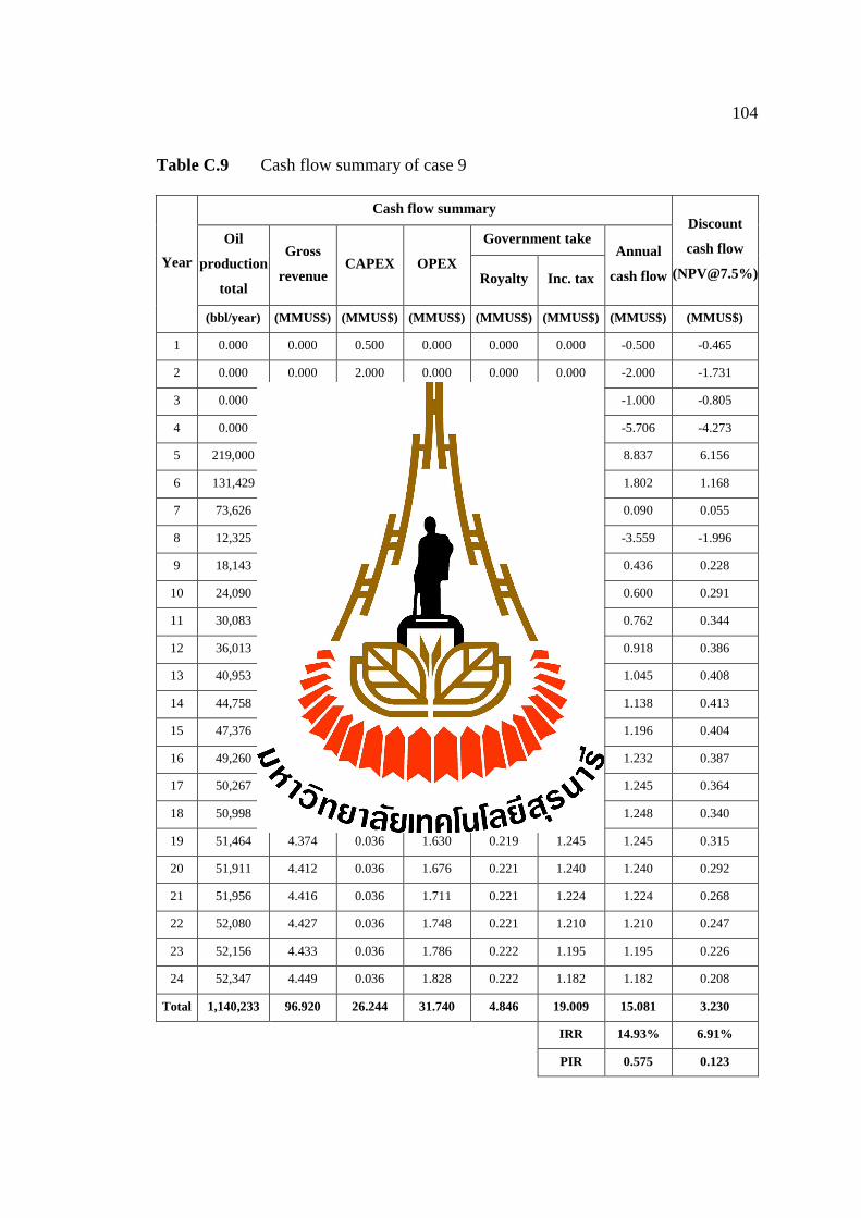
104
Table C.9 Cash flow summary of case 9
Year
Cash flow summary Discount
cash flow
Oil
production
total
Gross
revenue CAPEX OPEX
Government take Annual
cash flow Royalty Inc. tax
(bbl/year) (MMUS$) (MMUS$) (MMUS$) (MMUS$) (MMUS$) (MMUS$) (MMUS$)
1 0.000 0.000 0.500 0.000 0.000 0.000 -0.500 -0.465
2 0.000 0.000 2.000 0.000 0.000 0.000 -2.000 -1.731
3 0.000 0.000 1.000 0.000 0.000 0.000 -1.000 -0.805
4 0.000 0.000 22.131 0.000 0.000 0.000 -5.706 -4.273
5 219,000 18.615 0.000 4.741 0.931 0.000 8.837 6.156
6 131,429 11.171 0.000 2.902 0.559 1.802 1.802 1.168
7 73,626 6.258 0.000 1.658 0.313 0.090 0.090 0.055
8 12,325 1.048 0.036 0.412 0.052 0.000 -3.559 -1.996
9 18,143 1.542 0.036 0.556 0.077 0.436 0.436 0.228
10 24,090 2.048 0.036 0.710 0.102 0.600 0.600 0.291
11 30,083 2.557 0.036 0.870 0.128 0.762 0.762 0.344
12 36,013 3.061 0.036 1.035 0.153 0.918 0.918 0.386
13 40,953 3.481 0.036 1.181 0.174 1.045 1.045 0.408
14 44,758 3.804 0.036 1.303 0.190 1.138 1.138 0.413
15 47,376 4.027 0.036 1.398 0.201 1.196 1.196 0.404
16 49,260 4.187 0.036 1.477 0.209 1.232 1.232 0.387
17 50,267 4.273 0.036 1.534 0.214 1.245 1.245 0.364
18 50,998 4.335 0.036 1.585 0.217 1.248 1.248 0.340
19 51,464 4.374 0.036 1.630 0.219 1.245 1.245 0.315
20 51,911 4.412 0.036 1.676 0.221 1.240 1.240 0.292
21 51,956 4.416 0.036 1.711 0.221 1.224 1.224 0.268
22 52,080 4.427 0.036 1.748 0.221 1.210 1.210 0.247
23 52,156 4.433 0.036 1.786 0.222 1.195 1.195 0.226
24 52,347 4.449 0.036 1.828 0.222 1.182 1.182 0.208
Total 1,140,233 96.920 26.244 31.740 4.846 19.009 15.081 3.230
IRR 14.93% 6.91%
PIR 0.575 0.123

105
Table C.10 Cash flow summary of case 10
Year
Cash flow summary Discount
cash flow
Oil
production
total
Gross
revenue CAPEX OPEX
Government take Annual
cash flow Royalty Inc. tax
(bbl/year) (MMUS$) (MMUS$) (MMUS$) (MMUS$) (MMUS$) (MMUS$) (MMUS$)
1 0.000 0.000 0.500 0.000 0.000 0.000 -0.500 -0.465
2 0.000 0.000 2.000 0.000 0.000 0.000 -2.000 -1.731
3 0.000 0.000 1.000 0.000 0.000 0.000 -1.000 -0.805
4 0.000 0.000 22.131 0.000 0.000 0.000 -5.706 -4.273
5 219,000 18.615 0.000 4.741 0.931 0.000 8.837 6.156
6 131,429 11.171 0.000 2.902 0.559 1.802 1.802 1.168
7 73,626 6.258 0.000 1.658 0.313 0.090 0.090 0.055
8 16,901 1.437 0.073 0.649 0.072 0.000 -3.463 -1.942
9 35,377 3.007 0.073 1.095 0.150 0.845 0.845 0.441
10 59,888 5.090 0.073 1.702 0.255 1.530 1.530 0.743
11 73,000 6.205 0.073 2.056 0.310 1.883 1.883 0.850
12 73,200 6.222 0.073 2.103 0.311 1.868 1.868 0.784
13 73,000 6.205 0.073 2.139 0.310 1.841 1.841 0.719
14 73,000 6.205 0.073 2.182 0.310 1.820 1.820 0.661
15 73,000 6.205 0.073 2.226 0.310 1.798 1.798 0.608
16 73,200 6.222 0.073 2.276 0.311 1.781 1.781 0.560
17 73,000 6.205 0.073 2.315 0.310 1.753 1.753 0.513
18 73,000 6.205 0.073 2.362 0.310 1.730 1.730 0.471
19 73,000 6.205 0.073 2.409 0.310 1.707 1.707 0.432
20 73,200 6.222 0.073 2.464 0.311 1.687 1.687 0.397
21 73,000 6.205 0.073 2.506 0.310 1.658 1.658 0.363
22 73,000 6.205 0.073 2.556 0.310 1.633 1.633 0.333
23 73,000 6.205 0.073 2.608 0.310 1.607 1.607 0.305
24 73,200 6.222 0.073 2.667 0.311 1.586 1.586 0.280
Total 1,559,021 132.517 26.867 45.616 6.626 28.620 24.788 6.620
IRR 19.95% 11.58%
PIR 0.923 0.246
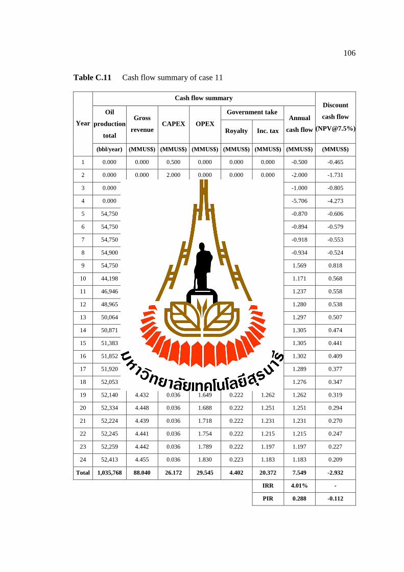
106
Table C.11 Cash flow summary of case 11
Year
Cash flow summary Discount
cash flow
Oil
production
total
Gross
revenue CAPEX OPEX
Government take Annual
cash flow Royalty Inc. tax
(bbl/year) (MMUS$) (MMUS$) (MMUS$) (MMUS$) (MMUS$) (MMUS$) (MMUS$)
1 0.000 0.000 0.500 0.000 0.000 0.000 -0.500 -0.465
2 0.000 0.000 2.000 0.000 0.000 0.000 -2.000 -1.731
3 0.000 0.000 1.000 0.000 0.000 0.000 -1.000 -0.805
4 0.000 0.000 22.131 0.000 0.000 0.000 -5.706 -4.273
5 54,750 4.654 0.000 1.185 0.233 0.000 -0.870 -0.606
6 54,750 4.654 0.000 1.209 0.233 0.000 -0.894 -0.579
7 54,750 4.654 0.000 1.233 0.233 0.000 -0.918 -0.553
8 54,900 4.667 0.000 1.261 0.233 0.000 -0.934 -0.524
9 54,750 4.654 0.000 1.283 0.233 1.569 1.569 0.818
10 44,198 3.757 0.036 1.190 0.188 1.171 1.171 0.568
11 46,946 3.990 0.036 1.281 0.200 1.237 1.237 0.558
12 48,965 4.162 0.036 1.357 0.208 1.280 1.280 0.538
13 50,064 4.255 0.036 1.412 0.213 1.297 1.297 0.507
14 50,871 4.324 0.036 1.461 0.216 1.305 1.305 0.474
15 51,383 4.368 0.036 1.504 0.218 1.305 1.305 0.441
16 51,852 4.407 0.036 1.547 0.220 1.302 1.302 0.409
17 51,920 4.413 0.036 1.579 0.221 1.289 1.289 0.377
18 52,053 4.425 0.036 1.615 0.221 1.276 1.276 0.347
19 52,140 4.432 0.036 1.649 0.222 1.262 1.262 0.319
20 52,334 4.448 0.036 1.688 0.222 1.251 1.251 0.294
21 52,224 4.439 0.036 1.718 0.222 1.231 1.231 0.270
22 52,245 4.441 0.036 1.754 0.222 1.215 1.215 0.247
23 52,259 4.442 0.036 1.789 0.222 1.197 1.197 0.227
24 52,413 4.455 0.036 1.830 0.223 1.183 1.183 0.209
Total 1,035,768 88.040 26.172 29.545 4.402 20.372 7.549 -2.932
IRR 4.01% -
PIR 0.288 -0.112

107
Table C.12 Cash flow summary of case 12
Year
Cash flow summary Discount
cash flow
Oil
production
total
Gross
revenue CAPEX OPEX
Government take Annual
cash flow Royalty Inc. tax
(bbl/year) (MMUS$) (MMUS$) (MMUS$) (MMUS$) (MMUS$) (MMUS$) (MMUS$)
1 0.000 0.000 0.500 0.000 0.000 0.000 -0.500 -0.465
2 0.000 0.000 2.000 0.000 0.000 0.000 -2.000 -1.731
3 0.000 0.000 1.000 0.000 0.000 0.000 -1.000 -0.805
4 0.000 0.000 22.131 0.000 0.000 0.000 -5.706 -4.273
5 54,750 4.654 0.000 1.185 0.233 0.000 -0.870 -0.606
6 54,750 4.654 0.000 1.209 0.233 0.000 -0.894 -0.579
7 54,750 4.654 0.000 1.233 0.233 0.000 -0.918 -0.553
8 54,900 4.667 0.000 1.261 0.233 0.000 -0.934 -0.524
9 54,750 4.654 0.000 1.283 0.233 1.569 1.569 0.818
10 52,732 4.482 0.073 1.427 0.224 1.379 1.379 0.669
11 54,750 4.654 0.073 1.505 0.233 1.422 1.422 0.642
12 54,900 4.667 0.073 1.539 0.233 1.411 1.411 0.592
13 54,750 4.654 0.073 1.565 0.233 1.391 1.391 0.543
14 54,750 4.654 0.073 1.597 0.233 1.376 1.376 0.500
15 54,750 4.654 0.073 1.629 0.233 1.360 1.360 0.460
16 54,900 4.667 0.073 1.666 0.233 1.347 1.347 0.424
17 54,750 4.654 0.073 1.695 0.233 1.327 1.327 0.388
18 54,750 4.654 0.073 1.728 0.233 1.310 1.310 0.356
19 54,750 4.654 0.073 1.763 0.233 1.293 1.293 0.327
20 54,900 4.667 0.073 1.803 0.233 1.279 1.279 0.301
21 54,750 4.654 0.073 1.834 0.233 1.257 1.257 0.275
22 54,750 4.654 0.073 1.871 0.233 1.239 1.239 0.252
23 54,750 4.654 0.073 1.908 0.233 1.220 1.220 0.231
24 54,900 4.666 0.073 1.951 0.233 1.204 1.204 0.212
Total 1,093,732 92.967 26.721 31.652 4.648 21.384 8.561 -2.544
IRR 4.50% #NUM!
PIR 0.320 -0.095
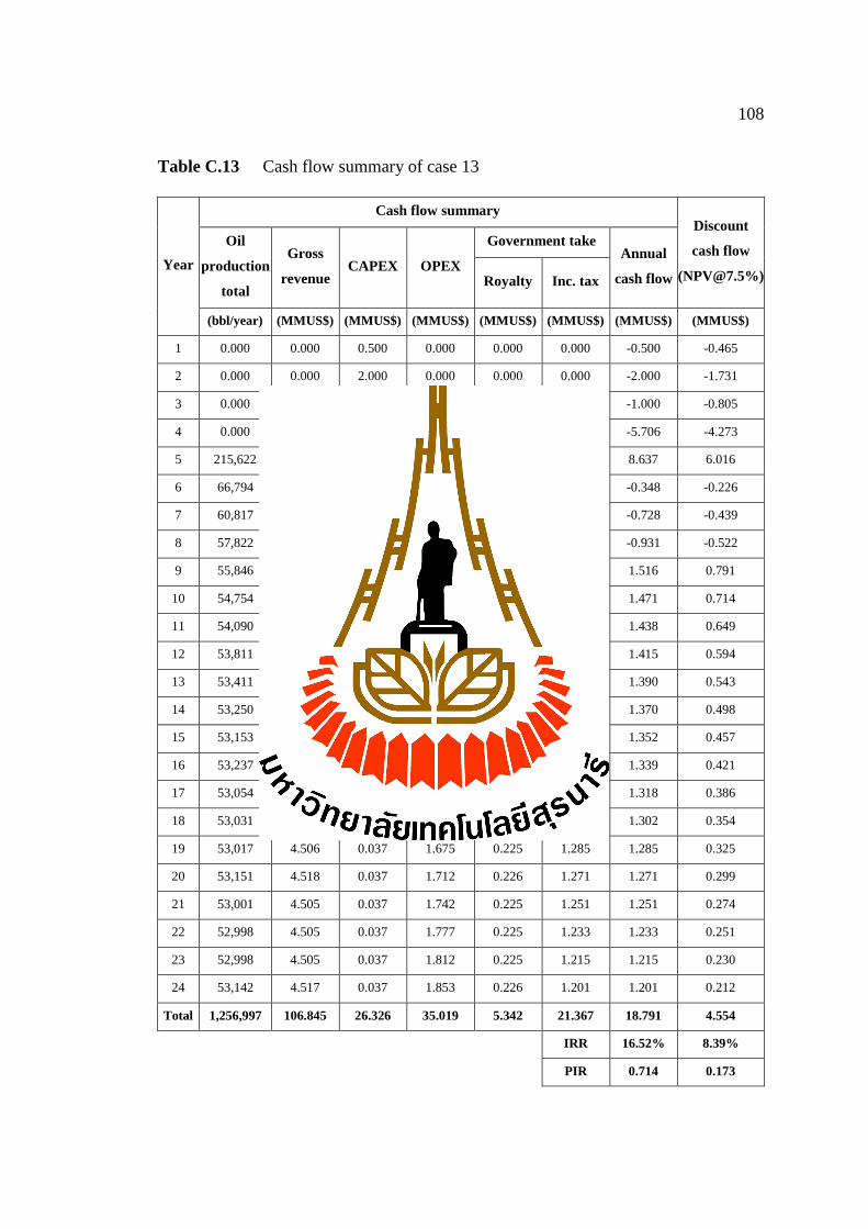
108
Table C.13 Cash flow summary of case 13
Year
Cash flow summary Discount
cash flow
Oil
production
total
Gross
revenue CAPEX OPEX
Government take Annual
cash flow Royalty Inc. tax
(bbl/year) (MMUS$) (MMUS$) (MMUS$) (MMUS$) (MMUS$) (MMUS$) (MMUS$)
1 0.000 0.000 0.500 0.000 0.000 0.000 -0.500 -0.465
2 0.000 0.000 2.000 0.000 0.000 0.000 -2.000 -1.731
3 0.000 0.000 1.000 0.000 0.000 0.000 -1.000 -0.805
4 0.000 0.000 22.131 0.000 0.000 0.000 -5.706 -4.273
5 215,622 18.328 0.000 4.668 0.916 0.000 8.637 6.016
6 66,794 5.677 0.037 1.599 0.284 0.000 -0.348 -0.226
7 60,817 5.169 0.037 1.496 0.258 0.000 -0.728 -0.439
8 57,822 4.915 0.037 1.458 0.246 0.000 -0.931 -0.522
9 55,846 4.747 0.037 1.440 0.237 1.516 1.516 0.791
10 54,754 4.654 0.037 1.443 0.233 1.471 1.471 0.714
11 54,090 4.598 0.037 1.456 0.230 1.438 1.438 0.649
12 53,811 4.574 0.037 1.478 0.229 1.415 1.415 0.594
13 53,411 4.540 0.037 1.497 0.227 1.390 1.390 0.543
14 53,250 4.526 0.037 1.523 0.226 1.370 1.370 0.498
15 53,153 4.518 0.037 1.551 0.226 1.352 1.352 0.457
16 53,237 4.525 0.037 1.584 0.226 1.339 1.339 0.421
17 53,054 4.510 0.037 1.611 0.225 1.318 1.318 0.386
18 53,031 4.508 0.037 1.642 0.225 1.302 1.302 0.354
19 53,017 4.506 0.037 1.675 0.225 1.285 1.285 0.325
20 53,151 4.518 0.037 1.712 0.226 1.271 1.271 0.299
21 53,001 4.505 0.037 1.742 0.225 1.251 1.251 0.274
22 52,998 4.505 0.037 1.777 0.225 1.233 1.233 0.251
23 52,998 4.505 0.037 1.812 0.225 1.215 1.215 0.230
24 53,142 4.517 0.037 1.853 0.226 1.201 1.201 0.212
Total 1,256,997 106.845 26.326 35.019 5.342 21.367 18.791 4.554
IRR 16.52% 8.39%
PIR 0.714 0.173

109
Table C.14 Cash flow summary of case 14
Year
Cash flow summary Discount
cash flow
Oil
production
total
Gross
revenue CAPEX OPEX
Government take Annual
cash flow Royalty Inc. tax
(bbl/year) (MMUS$) (MMUS$) (MMUS$) (MMUS$) (MMUS$) (MMUS$) (MMUS$)
1 0.000 0.000 0.500 0.000 0.000 0.000 -0.500 -0.465
2 0.000 0.000 2.000 0.000 0.000 0.000 -2.000 -1.731
3 0.000 0.000 1.000 0.000 0.000 0.000 -1.000 -0.805
4 0.000 0.000 22.131 0.000 0.000 0.000 -5.706 -4.273
5 215,622 18.328 0.000 4.668 0.916 0.000 8.637 6.016
6 73,000 6.205 0.073 1.766 0.310 0.000 -0.051 -0.033
7 73,000 6.205 0.073 1.802 0.310 0.000 -0.086 -0.052
8 73,200 6.222 0.073 1.842 0.311 0.000 -0.111 -0.062
9 73,000 6.205 0.073 1.874 0.310 1.974 1.974 1.029
10 73,000 6.205 0.073 1.912 0.310 1.955 1.955 0.948
11 73,000 6.205 0.073 1.950 0.310 1.936 1.936 0.874
12 73,200 6.222 0.073 1.994 0.311 1.922 1.922 0.807
13 73,000 6.205 0.073 2.029 0.310 1.896 1.896 0.741
14 73,000 6.205 0.073 2.069 0.310 1.876 1.876 0.682
15 73,000 6.205 0.073 2.111 0.310 1.855 1.855 0.627
16 73,200 6.222 0.073 2.159 0.311 1.839 1.839 0.578
17 73,000 6.205 0.073 2.196 0.310 1.813 1.813 0.530
18 73,000 6.205 0.073 2.240 0.310 1.791 1.791 0.487
19 73,000 6.205 0.073 2.285 0.310 1.768 1.768 0.448
20 73,200 6.222 0.073 2.337 0.311 1.750 1.750 0.412
21 73,000 6.205 0.073 2.377 0.310 1.722 1.722 0.377
22 73,000 6.205 0.073 2.425 0.310 1.698 1.698 0.346
23 73,000 6.205 0.073 2.473 0.310 1.674 1.674 0.317
24 73,200 6.222 0.073 2.529 0.311 1.654 1.654 0.292
Total 1,603,622 136.308 27.021 45.038 6.815 29.125 28.308 8.091
IRR 21.68% 13.19%
PIR 1.048 0.299

110
Table C.15 Cash flow summary of case 15
Year
Cash flow summary Discount
cash flow
Oil
production
total
Gross
revenue CAPEX OPEX
Government take Annual
cash flow Royalty Inc. tax
(bbl/year) (MMUS$) (MMUS$) (MMUS$) (MMUS$) (MMUS$) (MMUS$) (MMUS$)
1 0.000 0.000 0.500 0.000 0.000 0.000 -0.500 -0.465
2 0.000 0.000 2.000 0.000 0.000 0.000 -2.000 -1.731
3 0.000 0.000 1.000 0.000 0.000 0.000 -1.000 -0.805
4 0.000 0.000 26.000 0.000 0.000 0.000 -9.040 -6.769
5 219,000 18.615 0.000 4.741 0.931 0.000 8.703 6.062
6 131,429 11.171 0.000 2.902 0.559 1.735 1.735 1.124
7 73,626 6.258 0.156 1.658 0.313 0.000 -0.004 -0.002
8 12,381 1.052 0.037 0.414 0.053 0.000 -3.717 -2.084
9 18,313 1.557 0.037 0.561 0.078 0.428 0.428 0.223
10 24,400 2.074 0.037 0.717 0.104 0.595 0.595 0.289
11 30,567 2.598 0.037 0.882 0.130 0.775 0.775 0.350
12 36,672 3.117 0.037 1.052 0.156 0.936 0.936 0.393
13 41,710 3.545 0.037 1.200 0.177 1.066 1.066 0.416
14 45,533 3.870 0.037 1.323 0.194 1.158 1.158 0.421
15 48,152 4.093 0.037 1.419 0.205 1.216 1.216 0.411
16 50,032 4.253 0.037 1.498 0.213 1.253 1.253 0.394
17 51,013 4.336 0.037 1.555 0.217 1.264 1.264 0.370
18 51,739 4.398 0.037 1.606 0.220 1.268 1.268 0.345
19 52,203 4.437 0.037 1.652 0.222 1.264 1.264 0.320
20 52,634 4.474 0.037 1.697 0.224 1.258 1.258 0.296
21 52,676 4.477 0.037 1.732 0.224 1.242 1.242 0.272
22 52,796 4.488 0.037 1.771 0.224 1.228 1.228 0.250
23 52,869 4.494 0.037 1.808 0.225 1.212 1.212 0.230
24 53,061 4.510 0.037 1.851 0.226 1.199 1.199 0.211
Total 1,150,806 97.818 30.278 32.041 4.891 19.096 11.539 0.521
IRR 8.36% 0.80%
PIR 0.381 0.017

111
Table C.16 Cash flow summary of case 16
Year
Cash flow summary Discount
cash flow
Oil
production
total
Gross
revenue CAPEX OPEX
Government take Annual
cash flow Royalty Inc. tax
(bbl/year) (MMUS$) (MMUS$) (MMUS$) (MMUS$) (MMUS$) (MMUS$) (MMUS$)
1 0.000 0.000 0.500 0.000 0.000 0.000 -0.500 -0.465
2 0.000 0.000 2.000 0.000 0.000 0.000 -2.000 -1.731
3 0.000 0.000 1.000 0.000 0.000 0.000 -1.000 -0.805
4 0.000 0.000 26.000 0.000 0.000 0.000 -9.040 -6.769
5 219,000 18.615 0.000 4.741 0.931 0.000 8.703 6.062
6 131,429 11.171 0.000 2.902 0.559 1.735 1.735 1.124
7 73,626 6.258 0.156 1.658 0.313 0.000 -0.004 -0.002
8 16,969 1.442 0.073 0.551 0.072 0.000 -3.520 -1.974
9 35,698 3.034 0.073 1.000 0.152 0.892 0.892 0.465
10 60,518 5.144 0.073 1.614 0.257 1.587 1.587 0.770
11 73,000 6.205 0.073 1.950 0.310 1.936 1.936 0.874
12 73,200 6.222 0.073 1.994 0.311 1.922 1.922 0.807
13 73,000 6.205 0.073 2.029 0.310 1.896 1.896 0.741
14 73,000 6.205 0.073 2.069 0.310 1.876 1.876 0.682
15 73,000 6.205 0.073 2.111 0.310 1.855 1.855 0.627
16 73,200 6.222 0.073 2.159 0.311 1.839 1.839 0.578
17 73,000 6.205 0.073 2.196 0.310 1.813 1.813 0.530
18 73,000 6.205 0.073 2.240 0.310 1.791 1.791 0.487
19 73,000 6.205 0.073 2.285 0.310 1.768 1.768 0.448
20 73,200 6.222 0.073 2.337 0.311 1.750 1.750 0.412
21 73,000 6.205 0.073 2.377 0.310 1.722 1.722 0.377
22 73,000 6.205 0.073 2.425 0.310 1.698 1.698 0.346
23 73,000 6.205 0.073 2.473 0.310 1.674 1.674 0.317
24 73,200 6.222 0.073 2.529 0.311 1.654 1.654 0.292
Total 1,560,039 132.603 30.900 43.640 6.630 29.410 22.050 4.193
IRR 13.39% 5.48%
PIR 0.714 0.136

112
Table C.17 Cash flow summary of case 17
Year
Cash flow summary Discount
cash flow
Oil
production
total
Gross
revenue CAPEX OPEX
Government take Annual
cash flow Royalty Inc. tax
(bbl/year) (MMUS$) (MMUS$) (MMUS$) (MMUS$) (MMUS$) (MMUS$) (MMUS$)
1 0.000 0.000 0.500 0.000 0.000 0.000 -0.500 -0.465
2 0.000 0.000 2.000 0.000 0.000 0.000 -2.000 -1.731
3 0.000 0.000 1.000 0.000 0.000 0.000 -1.000 -0.805
4 0.000 0.000 26.000 0.000 0.000 0.000 -9.040 -6.769
5 54,750 4.654 0.000 1.185 0.233 0.000 -1.004 -0.699
6 54,750 4.654 0.000 1.209 0.233 0.000 -1.028 -0.666
7 54,750 4.654 0.000 1.233 0.233 0.000 -1.052 -0.634
8 54,900 4.667 0.000 1.261 0.233 0.000 -1.068 -0.599
9 54,750 4.654 0.286 1.283 0.233 1.557 1.557 0.812
10 44,350 3.770 0.037 1.194 0.188 1.175 1.175 0.570
11 47,300 4.021 0.037 1.290 0.201 1.246 1.246 0.563
12 49,452 4.203 0.037 1.370 0.210 1.294 1.294 0.543
13 50,643 4.305 0.037 1.427 0.215 1.313 1.313 0.513
14 51,492 4.377 0.037 1.478 0.219 1.322 1.322 0.480
15 52,044 4.424 0.037 1.522 0.221 1.322 1.322 0.447
16 52,530 4.465 0.037 1.565 0.223 1.320 1.320 0.415
17 52,610 4.472 0.037 1.599 0.224 1.306 1.306 0.382
18 52,755 4.484 0.037 1.635 0.224 1.294 1.294 0.352
19 52,841 4.492 0.037 1.670 0.225 1.280 1.280 0.324
20 53,040 4.508 0.037 1.709 0.225 1.269 1.269 0.299
21 52,931 4.499 0.037 1.740 0.225 1.249 1.249 0.273
22 52,954 4.501 0.037 1.776 0.225 1.232 1.232 0.251
23 52,969 4.502 0.037 1.812 0.225 1.215 1.215 0.230
24 53,123 4.515 0.037 1.853 0.226 1.200 1.200 0.212
Total 1,044,935 88.819 30.334 29.810 4.441 20.594 3.901 -5.703
IRR 1.77% -
PIR 0.129 -0.188

113
Table C.18 Cash flow summary of case 18
Year
Cash flow summary Discount
cash flow
Oil
production
total
Gross
revenue CAPEX OPEX
Government take Annual
cash flow Royalty Inc. tax
(bbl/year) (MMUS$) (MMUS$) (MMUS$) (MMUS$) (MMUS$) (MMUS$) (MMUS$)
1 0.000 0.000 0.500 0.000 0.000 0.000 -0.500 -0.465
2 0.000 0.000 2.000 0.000 0.000 0.000 -2.000 -1.731
3 0.000 0.000 1.000 0.000 0.000 0.000 -1.000 -0.805
4 0.000 0.000 26.000 0.000 0.000 0.000 -9.040 -6.769
5 54,750 4.654 0.000 1.185 0.233 0.000 -1.004 -0.699
6 54,750 4.654 0.000 1.209 0.233 0.000 -1.028 -0.666
7 54,750 4.654 0.000 1.233 0.233 0.000 -1.052 -0.634
8 54,900 4.667 0.000 1.261 0.233 0.000 -1.068 -0.599
9 54,750 4.654 0.286 1.283 0.233 1.557 1.557 0.812
10 52,785 4.487 0.073 1.429 0.224 1.380 1.380 0.670
11 54,750 4.654 0.073 1.505 0.233 1.421 1.421 0.642
12 54,900 4.667 0.073 1.539 0.233 1.410 1.410 0.592
13 54,750 4.654 0.073 1.566 0.233 1.391 1.391 0.543
14 54,750 4.654 0.073 1.597 0.233 1.375 1.375 0.500
15 54,750 4.654 0.073 1.629 0.233 1.359 1.359 0.459
16 54,900 4.667 0.073 1.666 0.233 1.347 1.347 0.423
17 54,750 4.654 0.073 1.695 0.233 1.326 1.326 0.388
18 54,750 4.654 0.073 1.729 0.233 1.309 1.309 0.356
19 54,750 4.654 0.073 1.764 0.233 1.292 1.292 0.327
20 54,900 4.667 0.073 1.803 0.233 1.278 1.278 0.301
21 54,750 4.654 0.073 1.835 0.233 1.257 1.257 0.275
22 54,750 4.654 0.073 1.871 0.233 1.238 1.238 0.252
23 54,750 4.654 0.073 1.909 0.233 1.220 1.220 0.231
24 54,900 4.667 0.073 1.952 0.233 1.204 1.204 0.212
Total 1,093,785 92.972 30.883 31.661 4.649 21.366 4.673 -5.385
IRR 2.12% -
PIR 0.151 -0.174

114
Table C.19 Cash flow summary of case 19
Year
Cash flow summary Discount
cash flow
Oil
production
total
Gross
revenue CAPEX OPEX
Government take Annual
cash flow Royalty Inc. tax
(bbl/year) (MMUS$) (MMUS$) (MMUS$) (MMUS$) (MMUS$) (MMUS$) (MMUS$)
1 0.000 0.000 0.500 0.000 0.000 0.000 -0.500 -0.465
2 0.000 0.000 2.000 0.000 0.000 0.000 -2.000 -1.731
3 0.000 0.000 1.000 0.000 0.000 0.000 -1.000 -0.805
4 0.000 0.000 22.131 0.000 0.000 0.000 -5.706 -4.273
5 215,622 18.328 0.000 4.668 0.916 0.000 8.637 6.016
6 66,998 5.695 0.037 1.604 0.285 0.000 -0.337 -0.218
7 61,211 5.203 0.037 1.506 0.260 0.000 -0.706 -0.426
8 58,323 4.957 0.037 1.469 0.248 0.000 -0.903 -0.506
9 56,413 4.795 0.037 1.454 0.240 1.532 1.532 0.799
10 55,373 4.707 0.037 1.458 0.235 1.488 1.488 0.722
11 54,727 4.652 0.037 1.472 0.233 1.455 1.455 0.657
12 54,485 4.631 0.037 1.495 0.232 1.434 1.434 0.602
13 54,091 4.598 0.037 1.515 0.230 1.408 1.408 0.550
14 53,940 4.585 0.037 1.541 0.229 1.389 1.389 0.504
15 53,849 4.577 0.037 1.570 0.229 1.371 1.371 0.463
16 53,940 4.585 0.037 1.604 0.229 1.357 1.357 0.427
17 53,757 4.569 0.037 1.631 0.228 1.337 1.337 0.391
18 53,736 4.568 0.037 1.663 0.228 1.320 1.320 0.359
19 53,722 4.566 0.037 1.696 0.228 1.303 1.303 0.330
20 53,862 4.578 0.037 1.734 0.229 1.289 1.289 0.304
21 53,710 4.565 0.037 1.764 0.228 1.268 1.268 0.278
22 53,708 4.565 0.037 1.799 0.228 1.250 1.250 0.255
23 53,707 4.565 0.037 1.835 0.228 1.232 1.232 0.234
24 53,852 4.577 0.037 1.876 0.229 1.218 1.218 0.215
Total 1,269,025 107.867 26.335 35.353 5.393 21.651 19.136 4.681
IRR 16.72% 8.58%
PIR 0.727 0.178

115
Table C.20 Cash flow summary of case 20
Year
Cash flow summary Discount
cash flow
Oil
production
total
Gross
revenue CAPEX OPEX
Government take Annual
cash flow Royalty Inc. tax
(bbl/year) (MMUS$) (MMUS$) (MMUS$) (MMUS$) (MMUS$) (MMUS$) (MMUS$)
1 0.000 0.000 0.500 0.000 0.000 0.000 -0.500 -0.465
2 0.000 0.000 2.000 0.000 0.000 0.000 -2.000 -1.731
3 0.000 0.000 1.000 0.000 0.000 0.000 -1.000 -0.805
4 0.000 0.000 22.131 0.000 0.000 0.000 -5.706 -4.273
5 215,622 18.328 0.000 4.668 0.916 0.000 8.637 6.016
6 73,000 6.205 0.074 1.767 0.310 0.000 -0.052 -0.033
7 73,000 6.205 0.074 1.802 0.310 0.000 -0.087 -0.052
8 73,200 6.222 0.074 1.843 0.311 0.000 -0.112 -0.063
9 73,000 6.205 0.074 1.875 0.310 1.973 1.973 1.029
10 73,000 6.205 0.074 1.912 0.310 1.954 1.954 0.948
11 73,000 6.205 0.074 1.951 0.310 1.935 1.935 0.873
12 73,200 6.222 0.074 1.995 0.311 1.921 1.921 0.807
13 73,000 6.205 0.074 2.029 0.310 1.896 1.896 0.740
14 73,000 6.205 0.074 2.070 0.310 1.876 1.876 0.681
15 73,000 6.205 0.074 2.111 0.310 1.855 1.855 0.627
16 73,200 6.222 0.074 2.159 0.311 1.839 1.839 0.578
17 73,000 6.205 0.074 2.197 0.310 1.812 1.812 0.530
18 73,000 6.205 0.074 2.241 0.310 1.790 1.790 0.487
19 73,000 6.205 0.074 2.285 0.310 1.768 1.768 0.447
20 73,200 6.222 0.074 2.337 0.311 1.750 1.750 0.412
21 73,000 6.205 0.074 2.378 0.310 1.722 1.722 0.377
22 73,000 6.205 0.074 2.425 0.310 1.698 1.698 0.346
23 73,000 6.205 0.074 2.474 0.310 1.674 1.674 0.317
24 73,200 6.222 0.074 2.530 0.311 1.654 1.654 0.292
Total 1,603,622 136.308 27.030 45.047 6.815 29.117 28.298 8.087
IRR 21.67% 13.18%
PIR 1.047 0.299

116
Table C.21 Cash flow summary of case 21
Year
Cash flow summary Discount
cash flow
Oil
production
total
Gross
revenue CAPEX OPEX
Government take Annual
cash flow Royalty Inc. tax
(bbl/year) (MMUS$) (MMUS$) (MMUS$) (MMUS$) (MMUS$) (MMUS$) (MMUS$)
1 0.000 0.000 0.500 0.000 0.000 0.000 -0.500 -0.465
2 0.000 0.000 2.000 0.000 0.000 0.000 -2.000 -1.731
3 0.000 0.000 1.000 0.000 0.000 0.000 -1.000 -0.805
4 0.000 0.000 26.000 0.000 0.000 0.000 -9.040 -6.769
5 219,000 18.615 0.000 4.741 0.931 0.000 8.703 6.062
6 131,429 11.171 0.000 2.902 0.559 1.735 1.735 1.124
7 73,626 6.258 0.156 1.658 0.313 0.000 -0.004 -0.002
8 12,435 1.057 0.037 0.415 0.053 0.000 -3.714 -2.083
9 18,483 1.571 0.037 0.565 0.079 0.432 0.432 0.225
10 24,715 2.101 0.037 0.725 0.105 0.604 0.604 0.293
11 31,062 2.640 0.037 0.895 0.132 0.788 0.788 0.356
12 37,342 3.174 0.037 1.069 0.159 0.955 0.955 0.401
13 42,473 3.610 0.037 1.220 0.181 1.086 1.086 0.424
14 46,314 3.937 0.037 1.344 0.197 1.179 1.179 0.428
15 48,922 4.158 0.037 1.440 0.208 1.237 1.237 0.418
16 50,784 4.317 0.037 1.519 0.216 1.272 1.272 0.400
17 51,770 4.400 0.037 1.576 0.220 1.284 1.284 0.375
18 52,482 4.461 0.037 1.628 0.223 1.287 1.287 0.350
19 52,936 4.500 0.037 1.673 0.225 1.282 1.282 0.324
20 53,366 4.536 0.037 1.719 0.227 1.276 1.276 0.300
21 53,403 4.539 0.037 1.755 0.227 1.260 1.260 0.276
22 53,513 4.549 0.037 1.793 0.227 1.246 1.246 0.254
23 53,584 4.555 0.037 1.831 0.228 1.229 1.229 0.233
24 53,775 4.571 0.037 1.874 0.229 1.216 1.216 0.214
Total 1,161,412 98.720 30.286 32.343 4.936 19.368 11.813 0.605
IRR 8.50% 0.93%
PIR 0.390 0.020

117
Table C.22 Cash flow summary of case 22
Year
Cash flow summary Discount
cash flow
Oil
production
total
Gross
revenue CAPEX OPEX
Government take Annual
cash flow Royalty Inc. tax
(bbl/year) (MMUS$) (MMUS$) (MMUS$) (MMUS$) (MMUS$) (MMUS$) (MMUS$)
1 0.000 0.000 0.500 0.000 0.000 0.000 -0.500 -0.465
2 0.000 0.000 2.000 0.000 0.000 0.000 -2.000 -1.731
3 0.000 0.000 1.000 0.000 0.000 0.000 -1.000 -0.805
4 0.000 0.000 26.000 0.000 0.000 0.000 -9.040 -6.769
5 219,000 18.615 0.000 4.741 0.931 0.000 8.703 6.062
6 131,429 11.171 0.000 2.902 0.559 1.735 1.735 1.124
7 73,626 6.258 0.156 1.658 0.313 0.000 -0.004 -0.002
8 17,036 1.448 0.074 0.552 0.072 0.000 -3.517 -1.972
9 36,019 3.062 0.074 1.008 0.153 0.900 0.900 0.470
10 61,162 5.199 0.074 1.629 0.260 1.605 1.605 0.779
11 73,000 6.205 0.074 1.951 0.310 1.935 1.935 0.873
12 73,200 6.222 0.074 1.995 0.311 1.921 1.921 0.807
13 73,000 6.205 0.074 2.029 0.310 1.896 1.896 0.740
14 73,000 6.205 0.074 2.070 0.310 1.876 1.876 0.681
15 73,000 6.205 0.074 2.111 0.310 1.855 1.855 0.627
16 73,200 6.222 0.074 2.159 0.311 1.839 1.839 0.578
17 73,000 6.205 0.074 2.197 0.310 1.812 1.812 0.530
18 73,000 6.205 0.074 2.241 0.310 1.790 1.790 0.487
19 73,000 6.205 0.074 2.285 0.310 1.768 1.768 0.447
20 73,200 6.222 0.074 2.337 0.311 1.750 1.750 0.412
21 73,000 6.205 0.074 2.378 0.310 1.722 1.722 0.377
22 73,000 6.205 0.074 2.425 0.310 1.698 1.698 0.346
23 73,000 6.205 0.074 2.474 0.310 1.674 1.674 0.317
24 73,200 6.222 0.074 2.530 0.311 1.654 1.654 0.292
Total 1,561,071 132.691 30.908 43.673 6.635 29.430 22.072 4.206
IRR 13.41% 5.50%
PIR 0.714 0.136

118
Table C.23 Cash flow summary of case 23
Year
Cash flow summary Discount
cash flow
Oil
production
total
Gross
revenue CAPEX OPEX
Government take Annual
cash flow Royalty Inc. tax
(bbl/year) (MMUS$) (MMUS$) (MMUS$) (MMUS$) (MMUS$) (MMUS$) (MMUS$)
1 0.000 0.000 0.500 0.000 0.000 0.000 -0.500 -0.465
2 0.000 0.000 2.000 0.000 0.000 0.000 -2.000 -1.731
3 0.000 0.000 1.000 0.000 0.000 0.000 -1.000 -0.805
4 0.000 0.000 26.000 0.000 0.000 0.000 -9.040 -6.769
5 54,750 4.654 0.000 1.185 0.233 0.000 -1.004 -0.699
6 54,750 4.654 0.000 1.209 0.233 0.000 -1.028 -0.666
7 54,750 4.654 0.000 1.233 0.233 0.000 -1.052 -0.634
8 54,900 4.667 0.000 1.261 0.233 0.000 -1.068 -0.599
9 54,750 4.654 0.286 1.283 0.233 1.557 1.557 0.812
10 44,503 3.783 0.037 1.198 0.189 1.179 1.179 0.572
11 47,653 4.051 0.037 1.299 0.203 1.256 1.256 0.567
12 49,941 4.245 0.037 1.382 0.212 1.307 1.307 0.549
13 51,209 4.353 0.037 1.442 0.218 1.328 1.328 0.519
14 52,126 4.431 0.037 1.494 0.222 1.339 1.339 0.486
15 52,704 4.480 0.037 1.540 0.224 1.340 1.340 0.453
16 53,221 4.524 0.037 1.584 0.226 1.338 1.338 0.421
17 53,306 4.531 0.037 1.618 0.227 1.325 1.325 0.387
18 53,453 4.543 0.037 1.655 0.227 1.312 1.312 0.357
19 53,545 4.551 0.037 1.691 0.228 1.298 1.298 0.329
20 53,749 4.569 0.037 1.730 0.228 1.286 1.286 0.303
21 53,640 4.559 0.037 1.762 0.228 1.266 1.266 0.277
22 53,663 4.561 0.037 1.798 0.228 1.249 1.249 0.254
23 53,678 4.563 0.037 1.834 0.228 1.232 1.232 0.233
24 53,834 4.576 0.037 1.876 0.229 1.217 1.217 0.215
Total 1,054,125 89.601 30.342 30.075 4.480 20.828 4.136 -5.635
IRR 1.87% -
PIR 0.136 -0.186

119
Table C.24 Cash flow summary of case 24
Year
Cash flow summary Discount
cash flow
Oil
production
total
Gross
revenue CAPEX OPEX
Government take Annual
cash flow Royalty Inc. tax
(bbl/year) (MMUS$) (MMUS$) (MMUS$) (MMUS$) (MMUS$) (MMUS$) (MMUS$)
1 0.000 0.000 0.500 0.000 0.000 0.000 -0.500 -0.465
2 0.000 0.000 2.000 0.000 0.000 0.000 -2.000 -1.731
3 0.000 0.000 1.000 0.000 0.000 0.000 -1.000 -0.805
4 0.000 0.000 26.000 0.000 0.000 0.000 -9.040 -6.769
5 54,750 4.654 0.000 1.185 0.233 0.000 -1.004 -0.699
6 54,750 4.654 0.000 1.209 0.233 0.000 -1.028 -0.666
7 54,750 4.654 0.000 1.233 0.233 0.000 -1.052 -0.634
8 54,900 4.667 0.000 1.261 0.233 0.000 -1.068 -0.599
9 54,750 4.654 0.286 1.283 0.233 1.557 1.557 0.812
10 52,852 4.492 0.074 1.431 0.225 1.382 1.382 0.670
11 54,750 4.654 0.074 1.506 0.233 1.421 1.421 0.641
12 54,900 4.667 0.074 1.540 0.233 1.410 1.410 0.592
13 54,750 4.654 0.074 1.566 0.233 1.391 1.391 0.543
14 54,750 4.654 0.074 1.598 0.233 1.375 1.375 0.500
15 54,750 4.654 0.074 1.630 0.233 1.359 1.359 0.459
16 54,900 4.667 0.074 1.667 0.233 1.346 1.346 0.423
17 54,750 4.654 0.074 1.696 0.233 1.326 1.326 0.388
18 54,750 4.654 0.074 1.729 0.233 1.309 1.309 0.356
19 54,750 4.654 0.074 1.764 0.233 1.292 1.292 0.327
20 54,900 4.667 0.074 1.804 0.233 1.278 1.278 0.301
21 54,750 4.654 0.074 1.835 0.233 1.256 1.256 0.275
22 54,750 4.654 0.074 1.872 0.233 1.238 1.238 0.252
23 54,750 4.654 0.074 1.909 0.233 1.219 1.219 0.231
24 54,900 4.667 0.074 1.953 0.233 1.203 1.203 0.212
Total 1,093,852 92.977 30.891 31.670 4.649 21.360 4.668 -5.386
IRR 2.11% #DIV/0!
PIR 0.151 -0.174
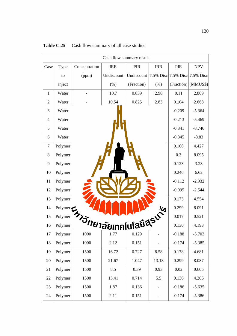
120
Table C.25 Cash flow summary of all case studies
Cash flow summary result
Case Type Concentration IRR PIR IRR PIR NPV
to (ppm) Undiscount Undiscount 7.5% Disc 7.5% Disc 7.5% Disc
inject
(%) (Fraction) (%) (Fraction) (MMUS$)
1 Water - 10.7 0.839 2.98 0.11 2.809
2 Water - 10.54 0.825 2.83 0.104 2.668
3 Water - 3.16 0.348 - -0.209 -5.364
4 Water - 3.06 0.336 - -0.213 -5.469
5 Water - 0.9 0.107 - -0.341 -8.746
6 Water - 0.81 0.096 - -0.345 -8.83
7 Polymer 600 16.31 0.701 8.2 0.168 4.427
8 Polymer 600 21.68 1.048 13.19 0.3 8.095
9 Polymer 600 14.93 0.575 6.91 0.123 3.23
10 Polymer 600 19.95 0.923 11.59 0.246 6.62
11 Polymer 600 4.01 0.288 - -0.112 -2.932
12 Polymer 600 4.5 0.32 - -0.095 -2.544
13 Polymer 1000 16.52 0.714 8.39 0.173 4.554
14 Polymer 1000 21.68 1.048 13.19 0.299 8.091
15 Polymer 1000 8.36 0.381 0.08 0.017 0.521
16 Polymer 1000 13.39 0.714 5.48 0.136 4.193
17 Polymer 1000 1.77 0.129 - -0.188 -5.703
18 Polymer 1000 2.12 0.151 - -0.174 -5.385
19 Polymer 1500 16.72 0.727 8.58 0.178 4.681
20 Polymer 1500 21.67 1.047 13.18 0.299 8.087
21 Polymer 1500 8.5 0.39 0.93 0.02 0.605
22 Polymer 1500 13.41 0.714 5.5 0.136 4.206
23 Polymer 1500 1.87 0.136 - -0.186 -5.635
24 Polymer 1500 2.11 0.151 - -0.174 -5.386

APPENDIX D
RESERVOIR SIMULATION RESULT
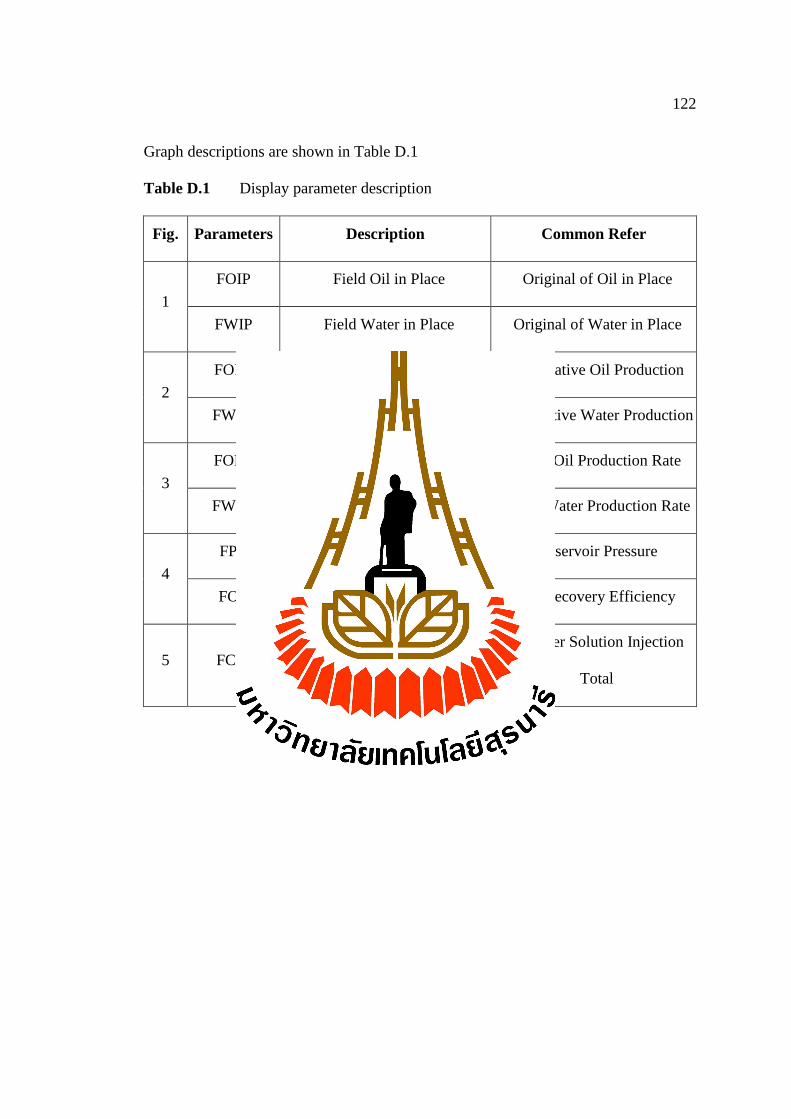
122
Graph descriptions are shown in Table D.1
Table D.1 Display parameter description
Fig. Parameters Description Common Refer
1
FOIP Field Oil in Place Original of Oil in Place
FWIP Field Water in Place Original of Water in Place
2
FOPT Field Oil Production Total Cumulative Oil Production
FWPT Field Water Production Total Cumulative Water Production
3
FOPR Field Oil Production Rate Daily Oil Production Rate
FWPR Field Water Production Rate Daily Water Production Rate
4
FPR Field Pressure Reservoir Pressure
FOE Field Oil Efficiency Oil Recovery Efficiency
5 FCIT Field Polymer Injection Total
Polymer Solution Injection
Total
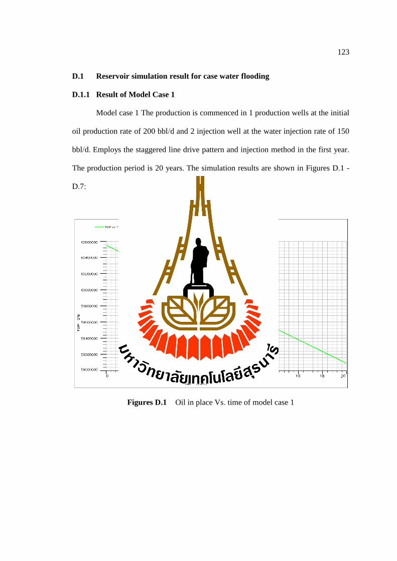
123
D.1 Reservoir simulation result for case water flooding
D.1.1 Result of Model Case 1
Model case 1 The production is commenced in 1 production wells at the initial
oil production rate of 200 bbl/d and 2 injection well at the water injection rate of 150
bbl/d. Employs the staggered line drive pattern and injection method in the first year.
The production period is 20 years. The simulation results are shown in Figures D.1 -
D.7:
Figures D.1 Oil in place Vs. time of model case 1
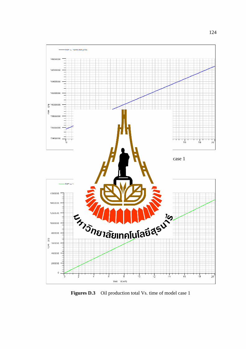
124
Figures D.2 Water in place Vs. time of model case 1
Figures D.3 Oil production total Vs. time of model case 1
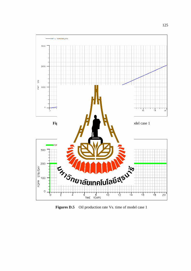
125
Figures D.4 Water production total Vs. time of model case 1
Figures D.5 Oil production rate Vs. time of model case 1
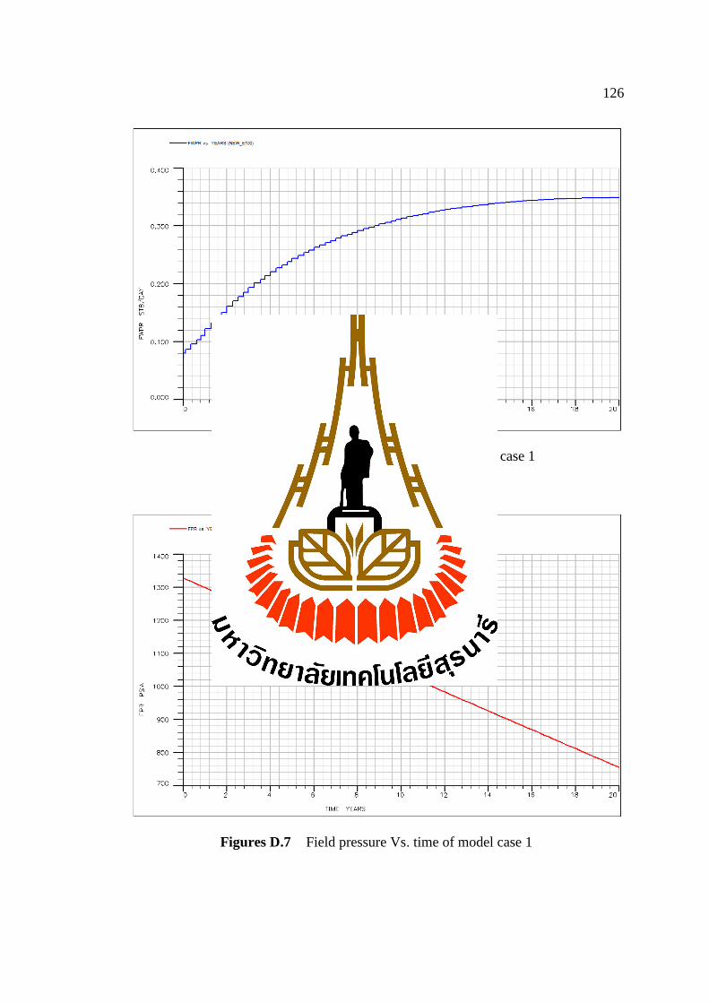
126
Figures D.6 Water production rate Vs. time of case 1
Figures D.7 Field pressure Vs. time of model case 1
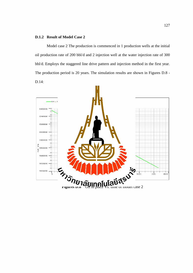
127
D.1.2 Result of Model Case 2
Model case 2 The production is commenced in 1 production wells at the initial
oil production rate of 200 bbl/d and 2 injection well at the water injection rate of 300
bbl/d. Employs the staggered line drive pattern and injection method in the first year.
The production period is 20 years. The simulation results are shown in Figures D.8 -
D.14:
Figures D.8 Oil in place Vs. time of model case 2
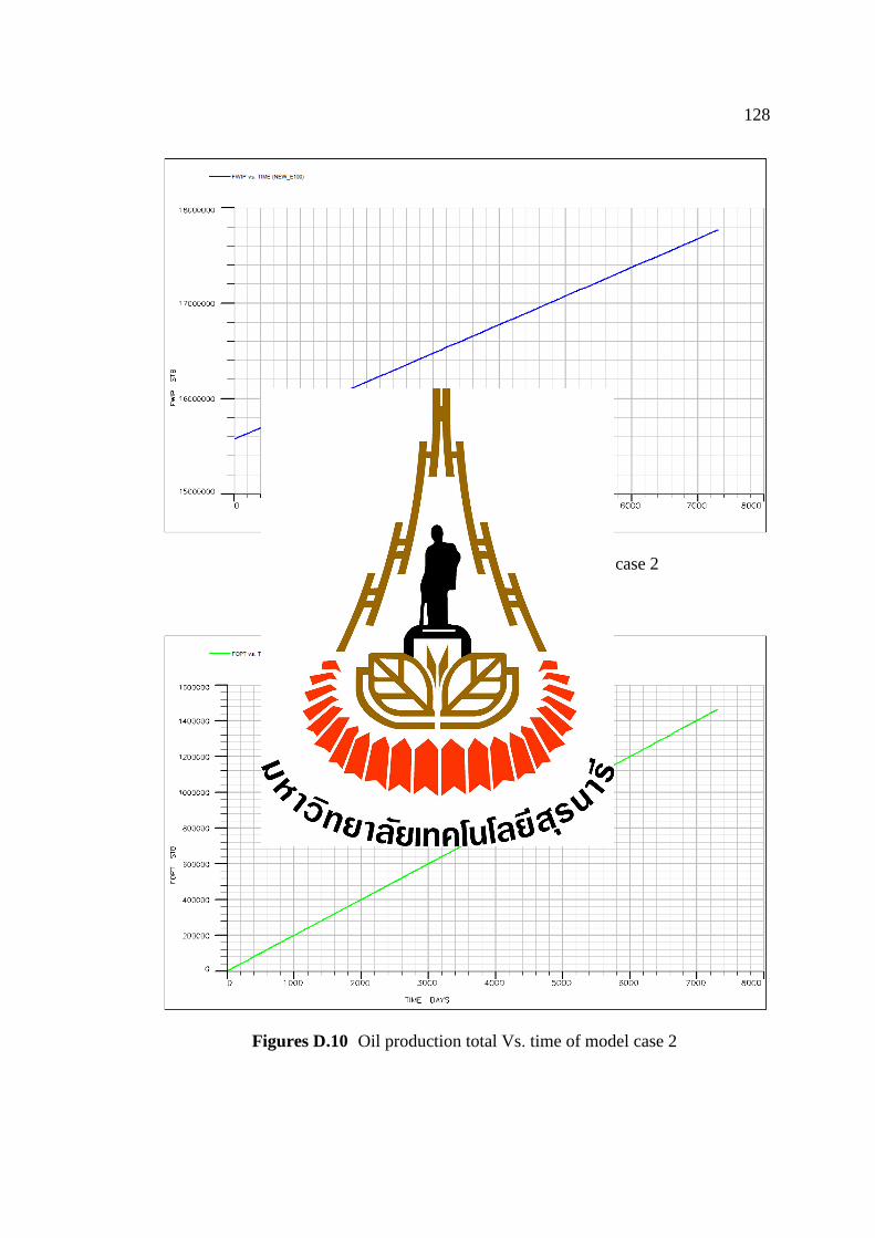
128
Figures D.9 Water in place Vs. time of model case 2
Figures D.10 Oil production total Vs. time of model case 2
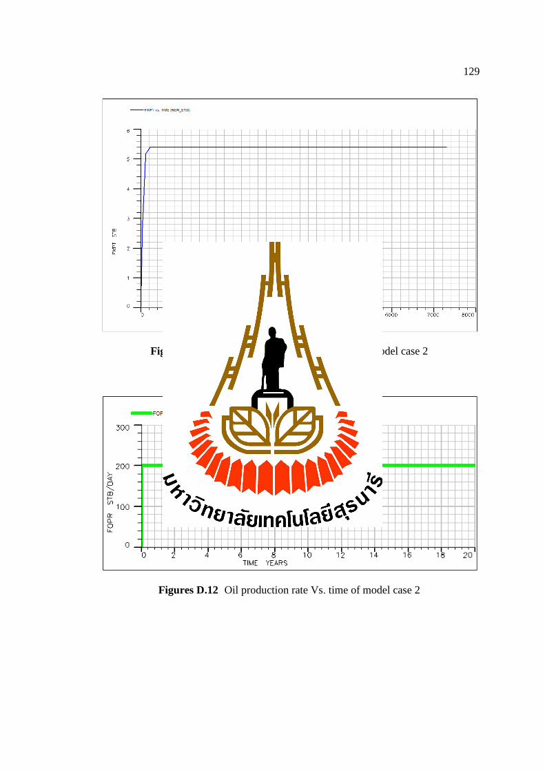
129
Figures D.11 Water production total Vs. time of model case 2
Figures D.12 Oil production rate Vs. time of model case 2
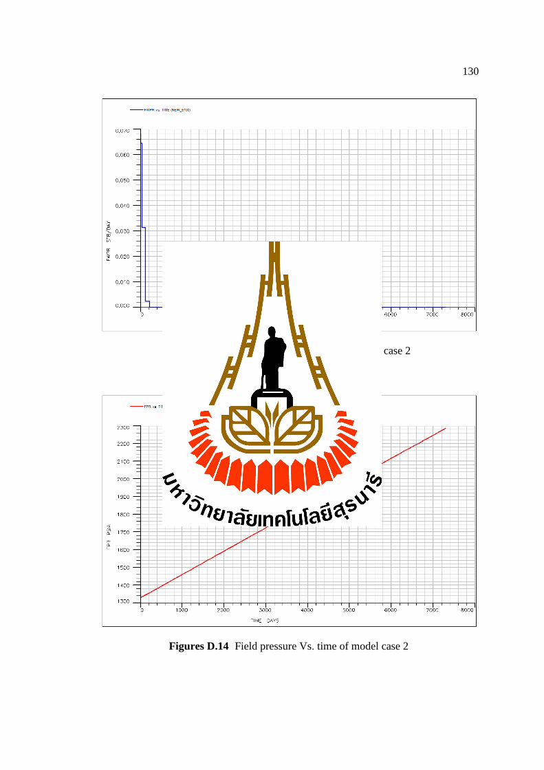
130
Figures D.13 Water production rate Vs. time of case 2
Figures D.14 Field pressure Vs. time of model case 2

131
D.1.3 Result of Model Case 3
Model case 3 The production is commenced in 1 production wells at the initial
oil production rate of 200 bbl/d and 2 injection well at the water injection rate of 150
bbl/d. Employs the staggered line drive pattern and injection method in the third year.
The production period is 20 years. The simulation results are shown in Figures D.15 -
D.21:
Figures D.15 Oil in place Vs. time of model case 3
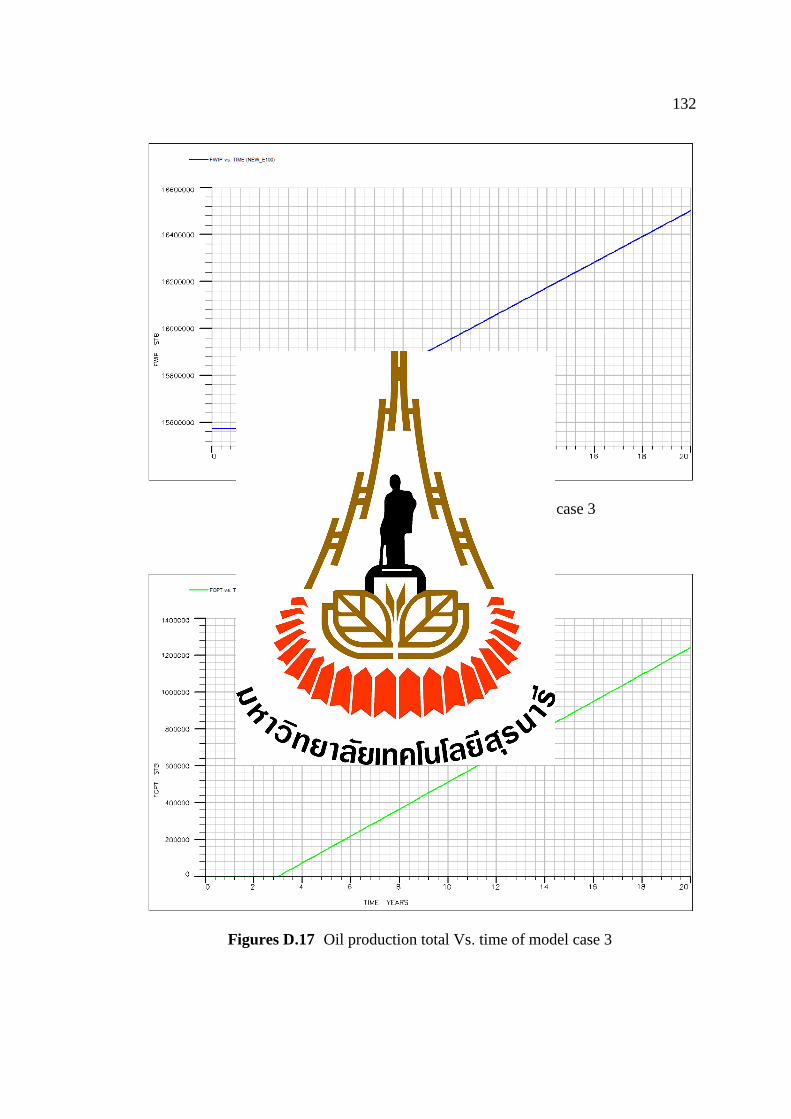
132
Figures D.16 Water in place Vs. time of model case 3
Figures D.17 Oil production total Vs. time of model case 3
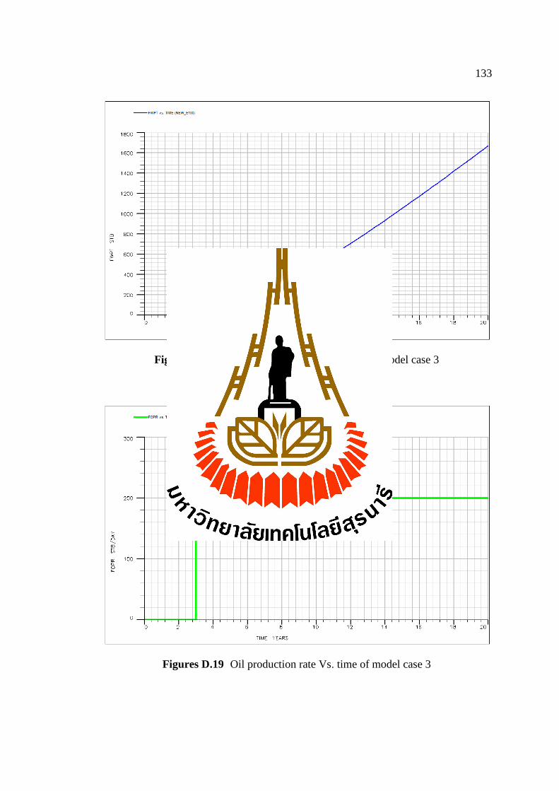
133
Figures D.18 Water production total Vs. time of model case 3
Figures D.19 Oil production rate Vs. time of model case 3
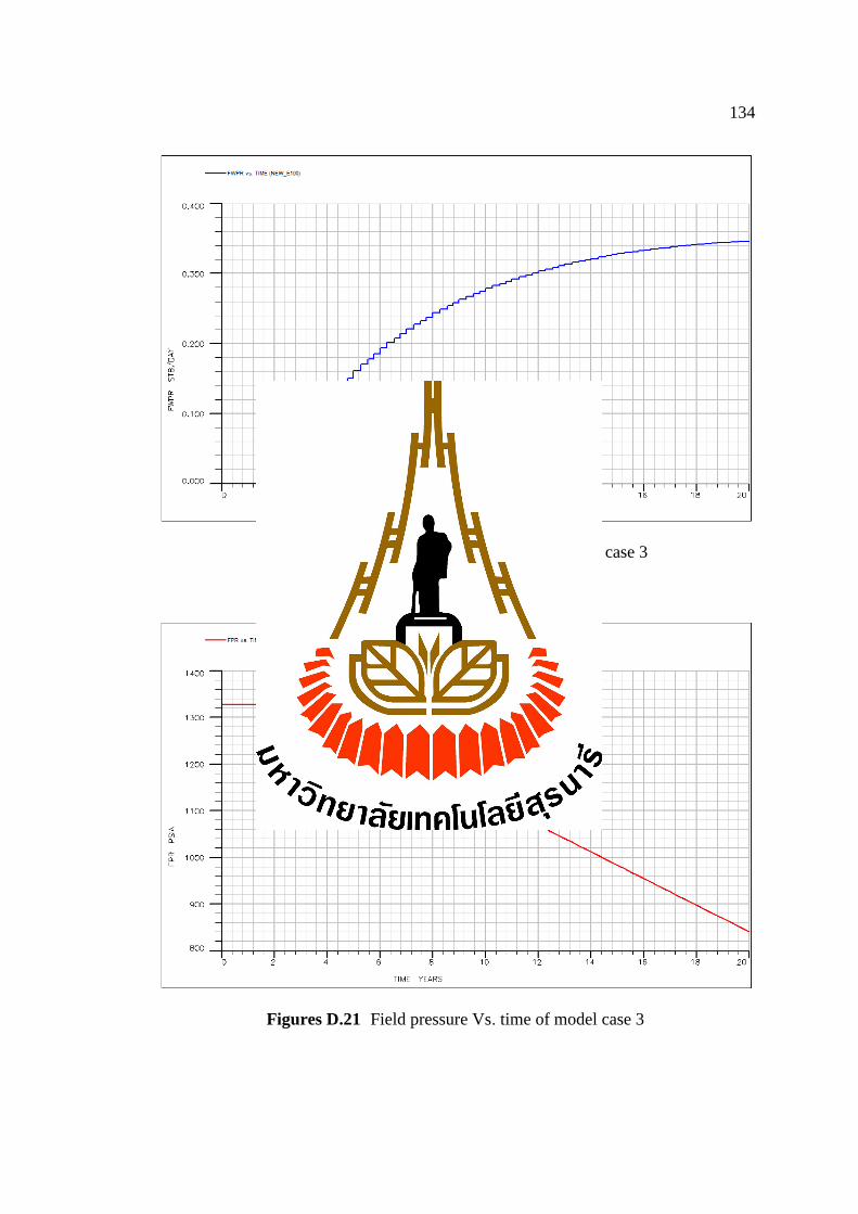
134
Figures D.20 Water production rate Vs. time of case 3
Figures D.21 Field pressure Vs. time of model case 3
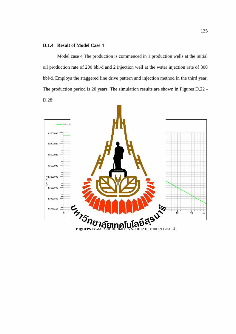
135
D.1.4 Result of Model Case 4
Model case 4 The production is commenced in 1 production wells at the initial
oil production rate of 200 bbl/d and 2 injection well at the water injection rate of 300
bbl/d. Employs the staggered line drive pattern and injection method in the third year.
The production period is 20 years. The simulation results are shown in Figures D.22 -
D.28:
Figures D.22 Oil in place Vs. time of model case 4
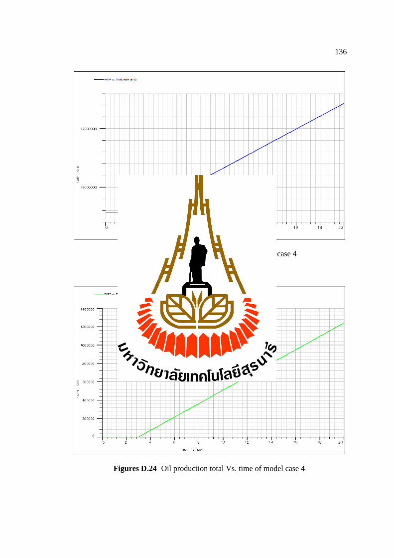
136
Figures D.23 Water in place Vs. time of model case 4
Figures D.24 Oil production total Vs. time of model case 4
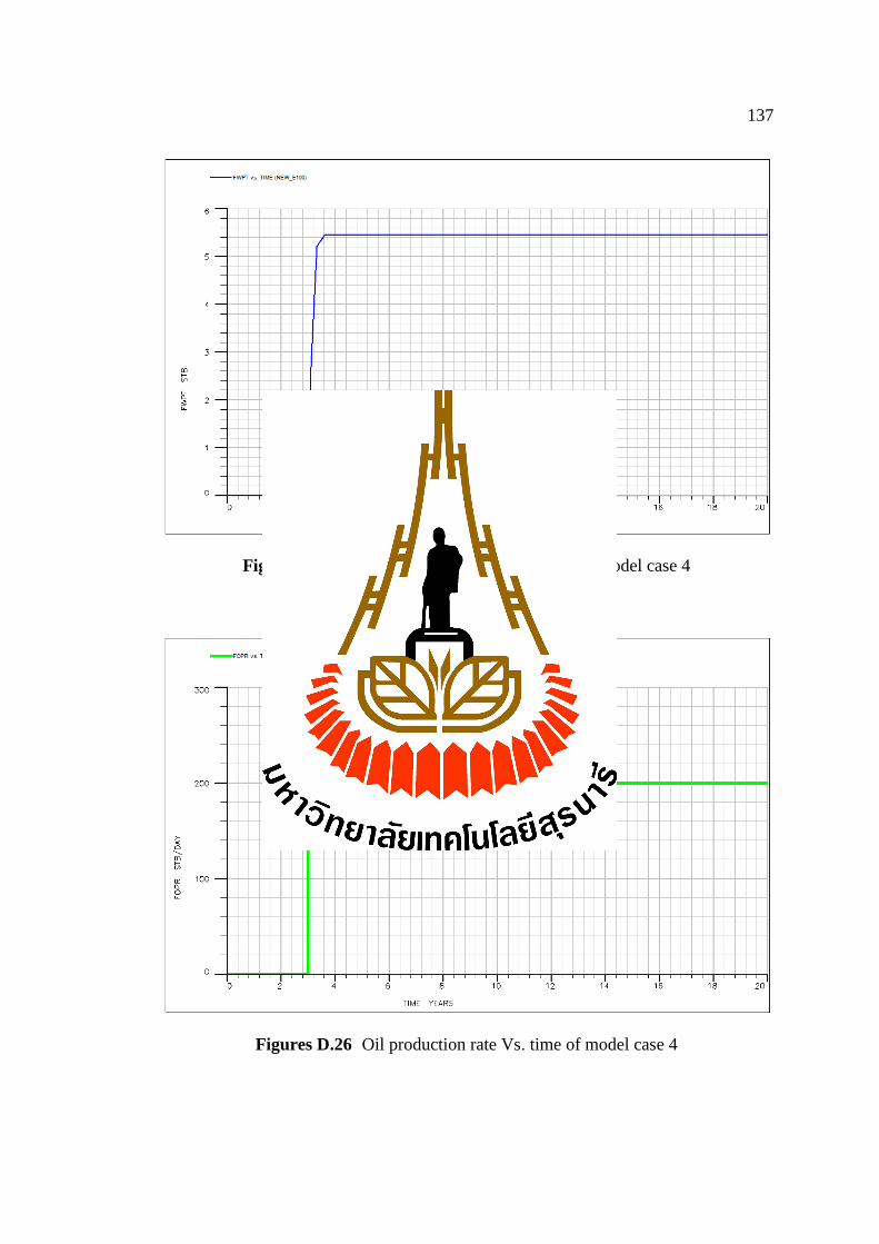
137
Figures D.25 Water production total Vs. time of model case 4
Figures D.26 Oil production rate Vs. time of model case 4
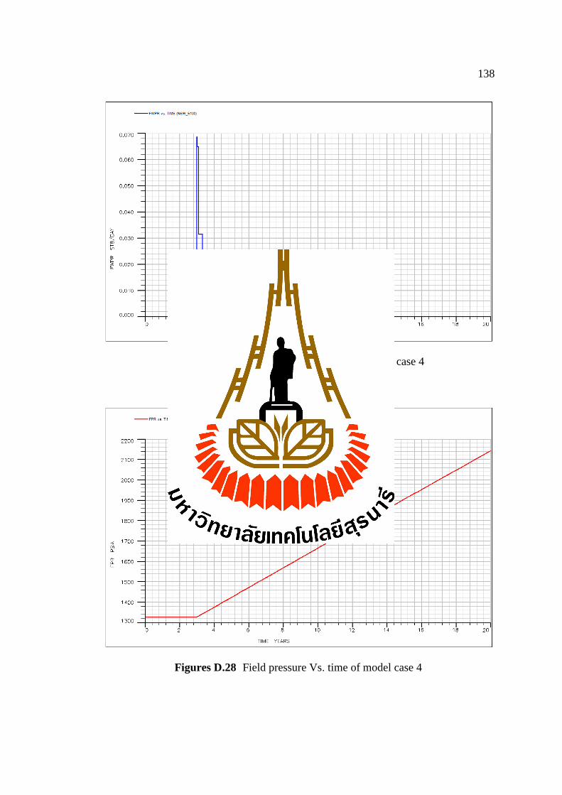
138
Figures D.27 Water production rate Vs. time of case 4
Figures D.28 Field pressure Vs. time of model case 4
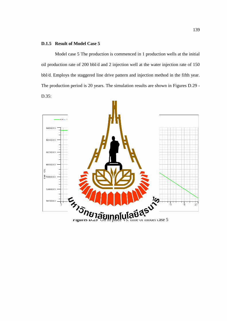
139
D.1.5 Result of Model Case 5
Model case 5 The production is commenced in 1 production wells at the initial
oil production rate of 200 bbl/d and 2 injection well at the water injection rate of 150
bbl/d. Employs the staggered line drive pattern and injection method in the fifth year.
The production period is 20 years. The simulation results are shown in Figures D.29 -
D.35:
Figures D.29 Oil in place Vs. time of model case 5
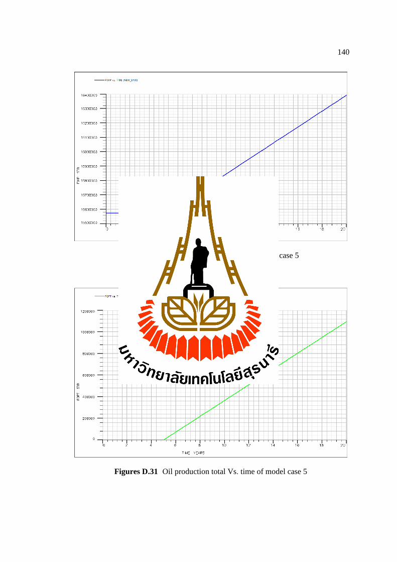
140
Figures D.30 Water in place Vs. time of model case 5
Figures D.31 Oil production total Vs. time of model case 5
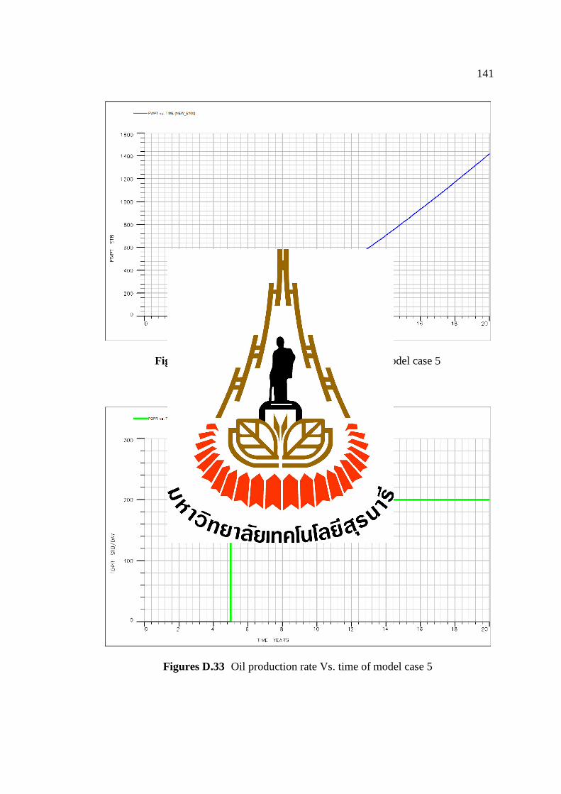
141
Figures D.32 Water production total Vs. time of model case 5
Figures D.33 Oil production rate Vs. time of model case 5
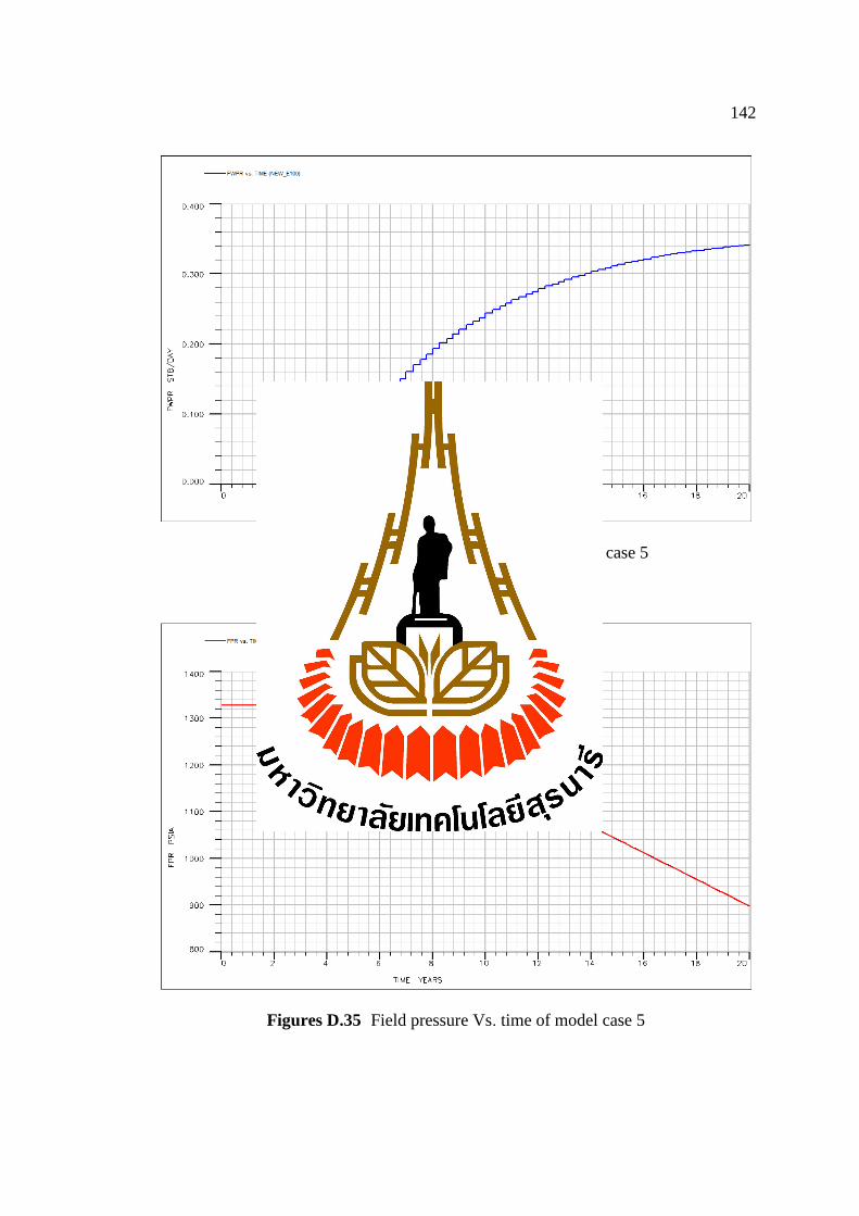
142
Figures D.34 Water production rate Vs. time of case 5
Figures D.35 Field pressure Vs. time of model case 5

143
D.1.6 Result of Model Case 6
Model case 6 The production is commenced in 1 production wells at the initial
oil production rate of 200 bbl/d and 2 injection well at the water injection rate of 300
bbl/d. Employs the staggered line drive pattern and injection method in the fifth year.
The production period is 20 years. The simulation results are shown in Figures D.36 -
D.42:
Figures D.36 Oil in place Vs. time of model case 6
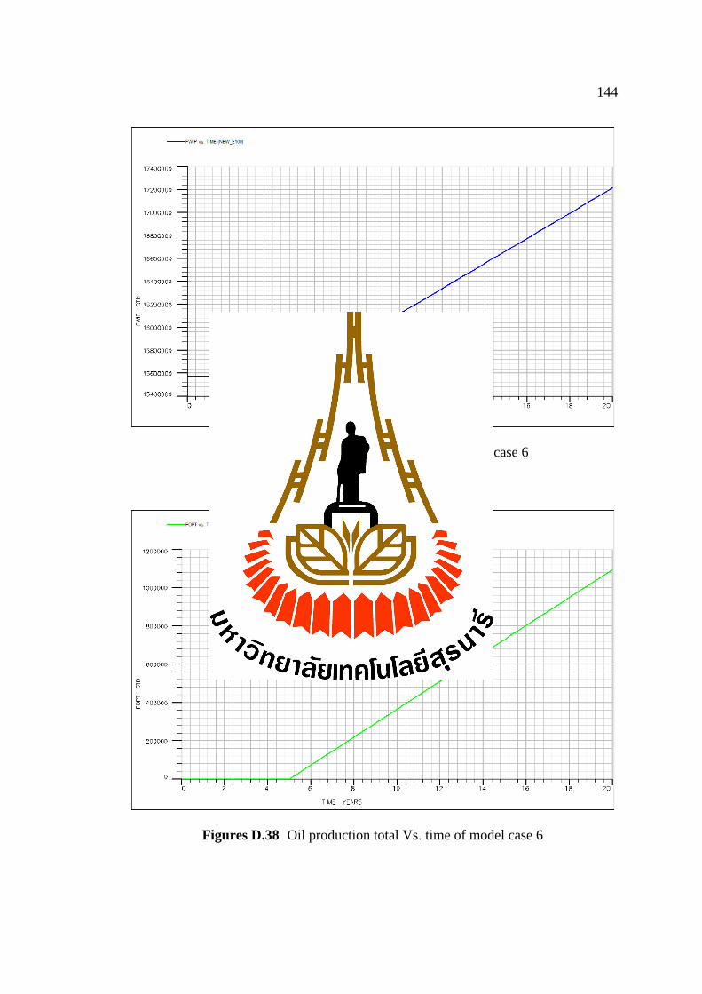
144
Figures D.37 Water in place Vs. time of model case 6
Figures D.38 Oil production total Vs. time of model case 6
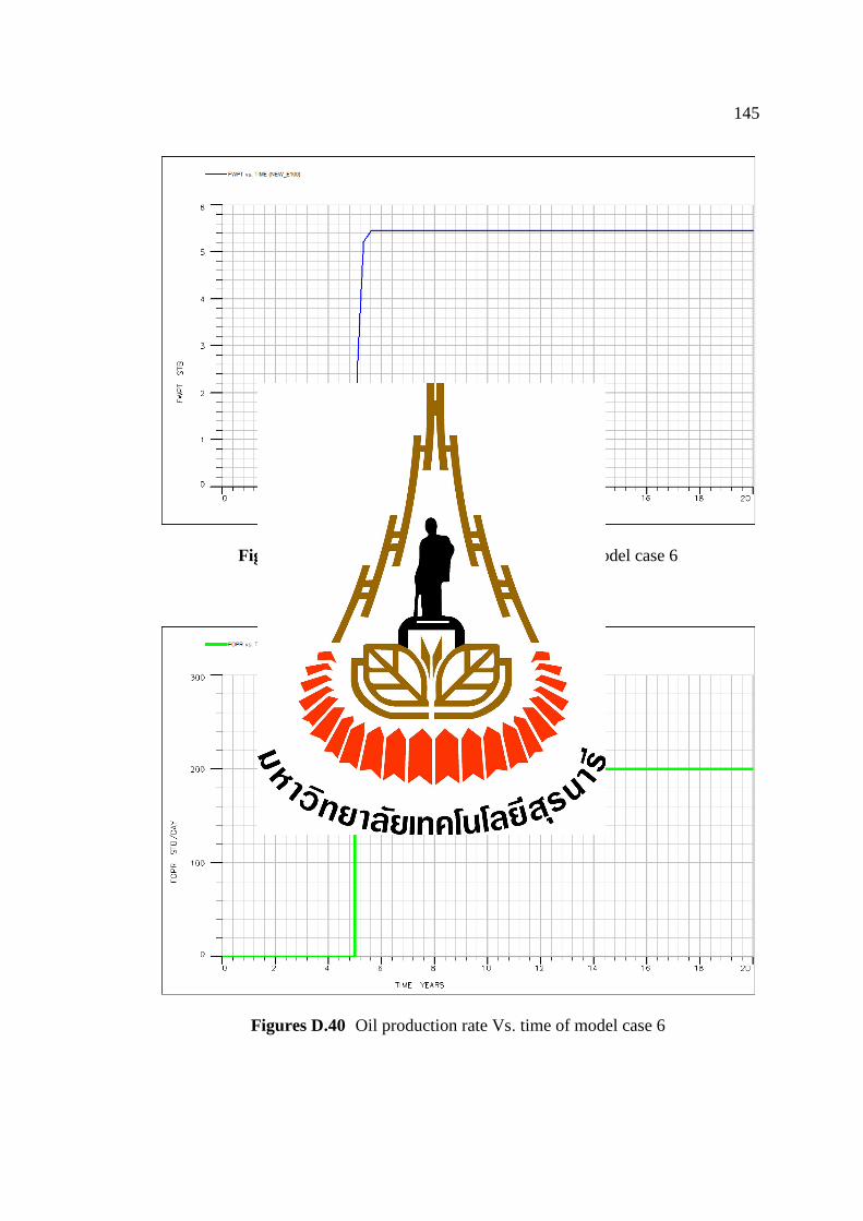
145
Figures D.39 Water production total Vs. time of model case 6
Figures D.40 Oil production rate Vs. time of model case 6
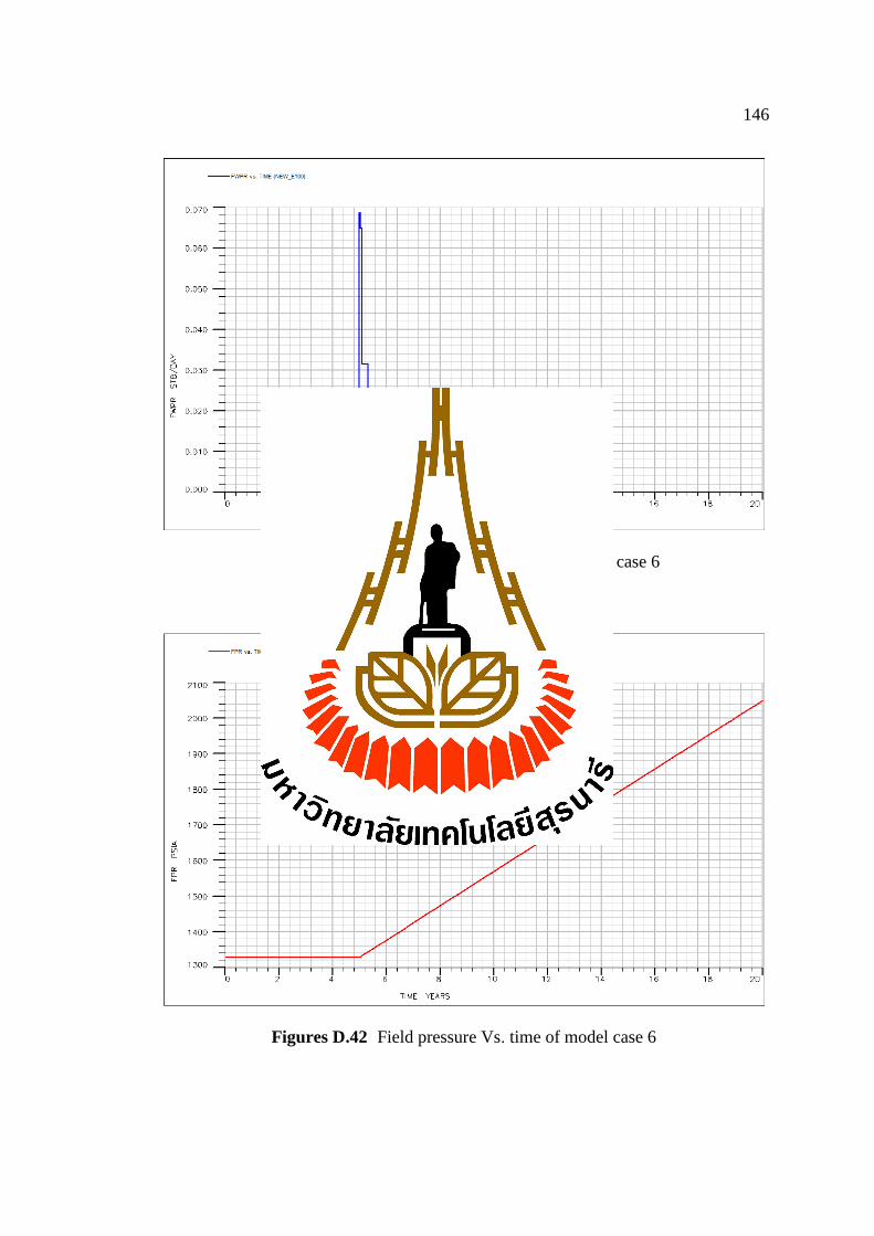
146
Figures D.41 Water production rate Vs. time of case 6
Figures D.42 Field pressure Vs. time of model case 6

147
D.2 Reservoir simulation result for case polymer flooding concentration 600 ppm
D.2.1 Result of Model Case 7
Model case 7 The production is commenced in 1 production wells at the initial
oil production rate of 200 bbl/d and 2 injection well at the polymer injection rate of
150 bbl/d in concentration 600 ppm. Employs the staggered line drive pattern and
injection method in the first year. The production period is 20 years. The simulation
results are shown in Figures D.44 - D.52:
Figures D.44 Oil in place Vs. time of model case 7
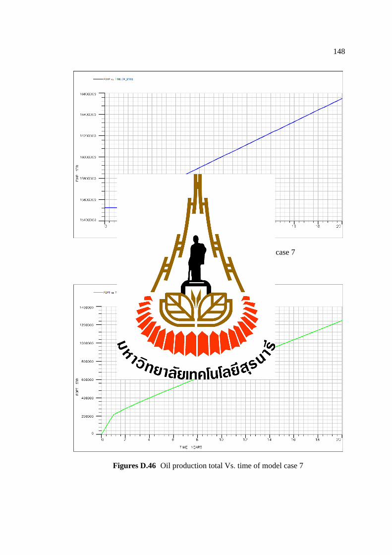
148
Figures D.45 Water in place Vs. time of model case 7
Figures D.46 Oil production total Vs. time of model case 7
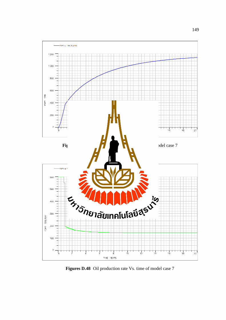
149
Figures D.47 Water production total Vs. time of model case 7
Figures D.48 Oil production rate Vs. time of model case 7
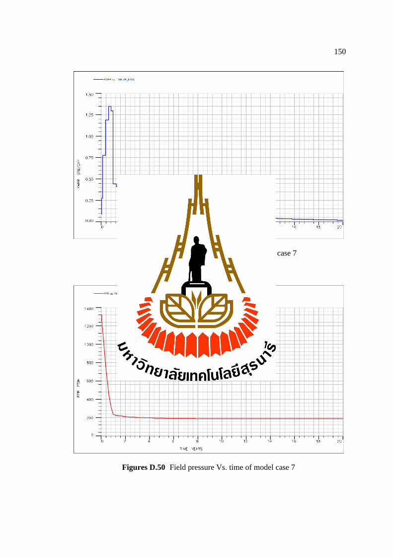
150
Figures D.49 Water production rate Vs. time of case 7
Figures D.50 Field pressure Vs. time of model case 7
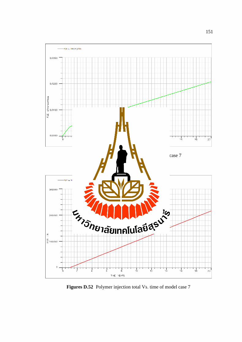
151
Figures D.51 Oil efficiency Vs. time of model case 7
Figures D.52 Polymer injection total Vs. time of model case 7
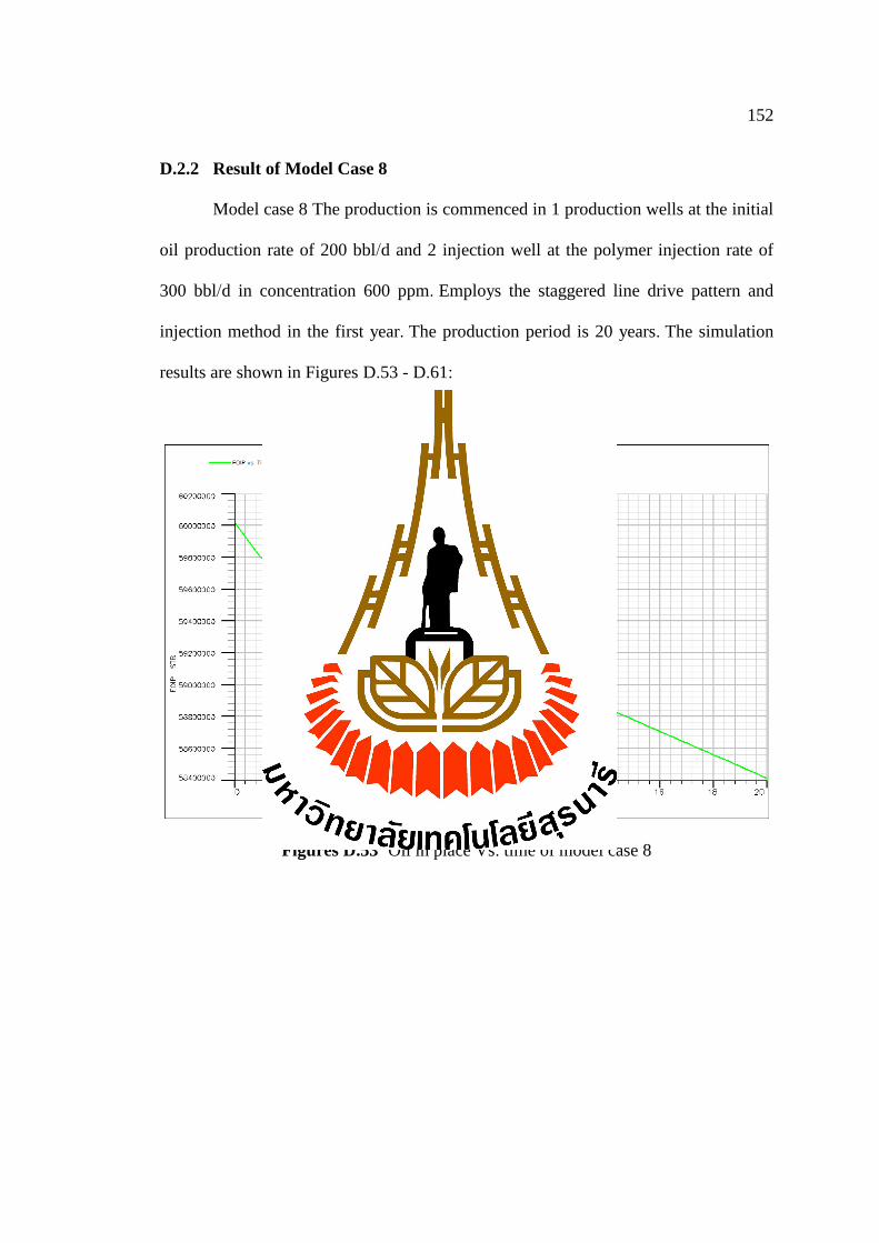
152
D.2.2 Result of Model Case 8
Model case 8 The production is commenced in 1 production wells at the initial
oil production rate of 200 bbl/d and 2 injection well at the polymer injection rate of
300 bbl/d in concentration 600 ppm. Employs the staggered line drive pattern and
injection method in the first year. The production period is 20 years. The simulation
results are shown in Figures D.53 - D.61:
Figures D.53 Oil in place Vs. time of model case 8
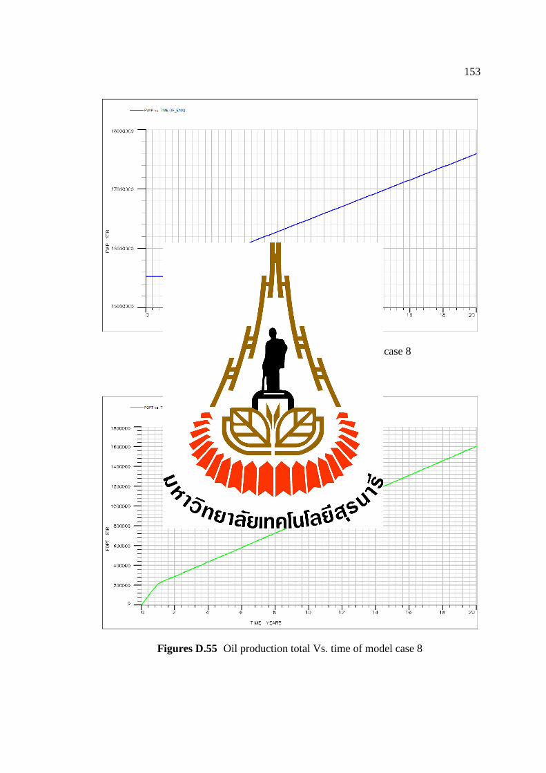
153
Figures D.54 Water in place Vs. time of model case 8
Figures D.55 Oil production total Vs. time of model case 8
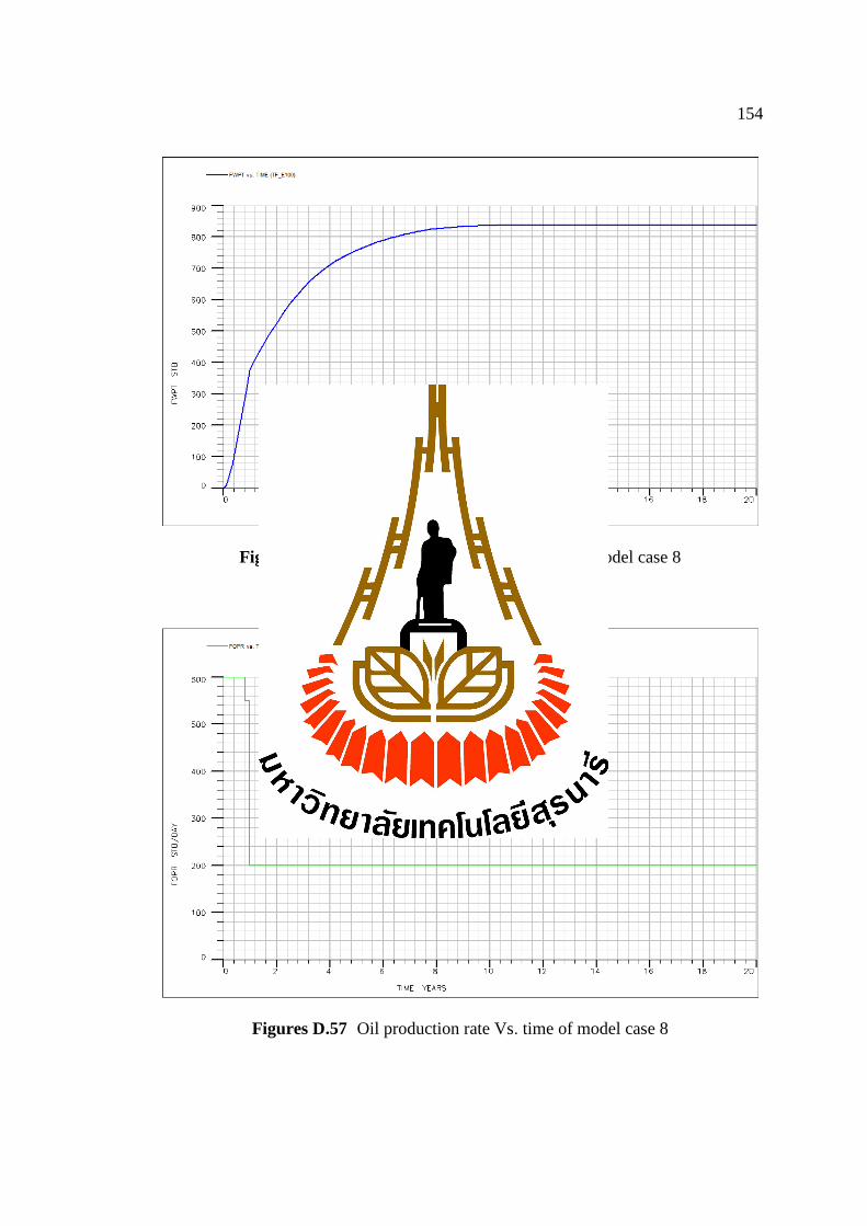
154
Figures D.56 Water production total Vs. time of model case 8
Figures D.57 Oil production rate Vs. time of model case 8
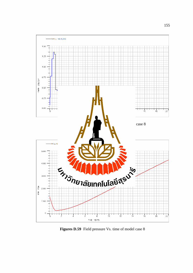
155
Figures D.58 Water production rate Vs. time of case 8
Figures D.59 Field pressure Vs. time of model case 8

156
Figures D.60 Oil efficiency Vs. time of model case 8
Figures D.61 Polymer injection total Vs. time of model case 8
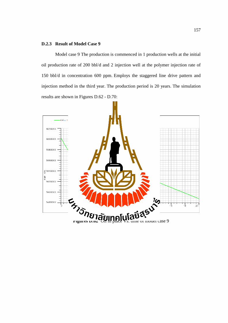
157
D.2.3 Result of Model Case 9
Model case 9 The production is commenced in 1 production wells at the initial
oil production rate of 200 bbl/d and 2 injection well at the polymer injection rate of
150 bbl/d in concentration 600 ppm. Employs the staggered line drive pattern and
injection method in the third year. The production period is 20 years. The simulation
results are shown in Figures D.62 - D.70:
Figures D.62 Oil in place Vs. time of model case 9
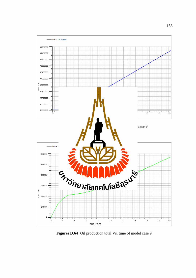
158
Figures D.63 Water in place Vs. time of model case 9
Figures D.64 Oil production total Vs. time of model case 9
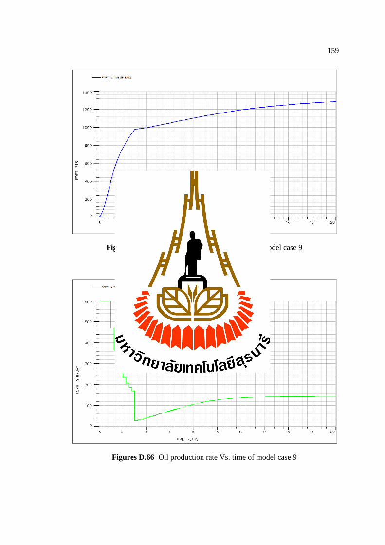
159
Figures D.65 Water production total Vs. time of model case 9
Figures D.66 Oil production rate Vs. time of model case 9
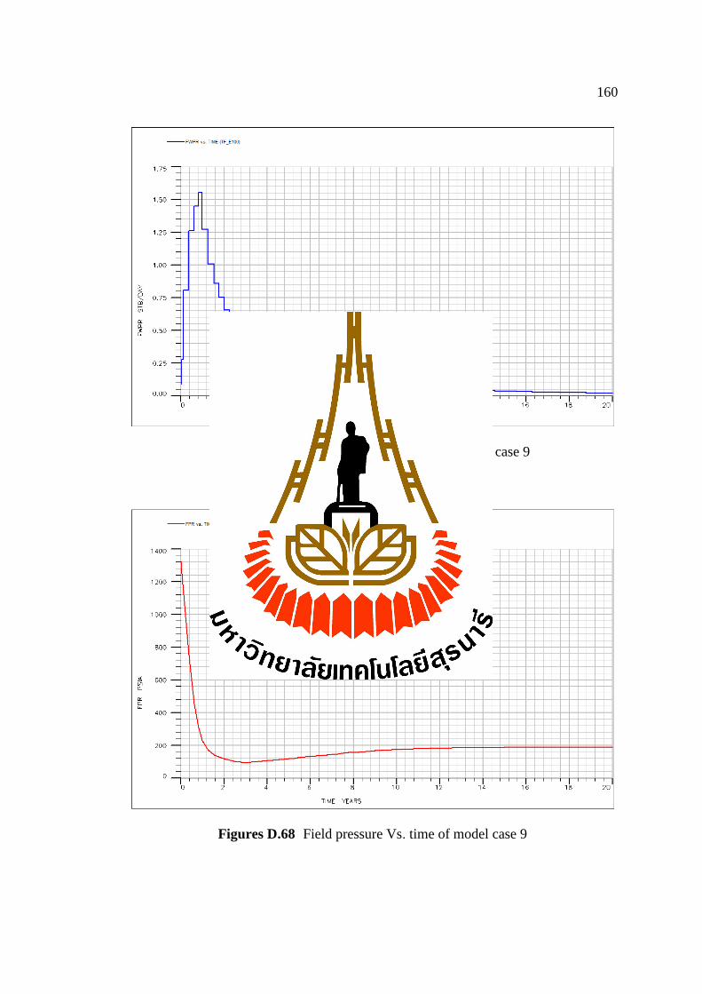
160
Figures D.67 Water production rate Vs. time of case 9
Figures D.68 Field pressure Vs. time of model case 9
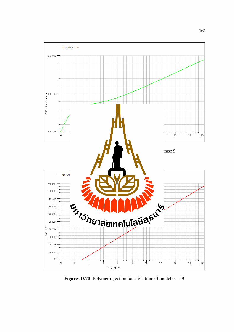
161
Figures D.69 Oil efficiency Vs. time of model case 9
Figures D.70 Polymer injection total Vs. time of model case 9

162
D.2.4 Result of Model Case 10
Model case 10 The production is commenced in 1 production wells at the
initial oil production rate of 200 bbl/d and 2 injection well at the polymer injection
rate of 300 bbl/d in concentration 600 ppm. Employs the staggered line drive pattern
and injection method in the third year. The production period is 20 years. The
simulation results are shown in Figures D.71 - D.79:
Figures D.71 Oil in place Vs. time of model case 10
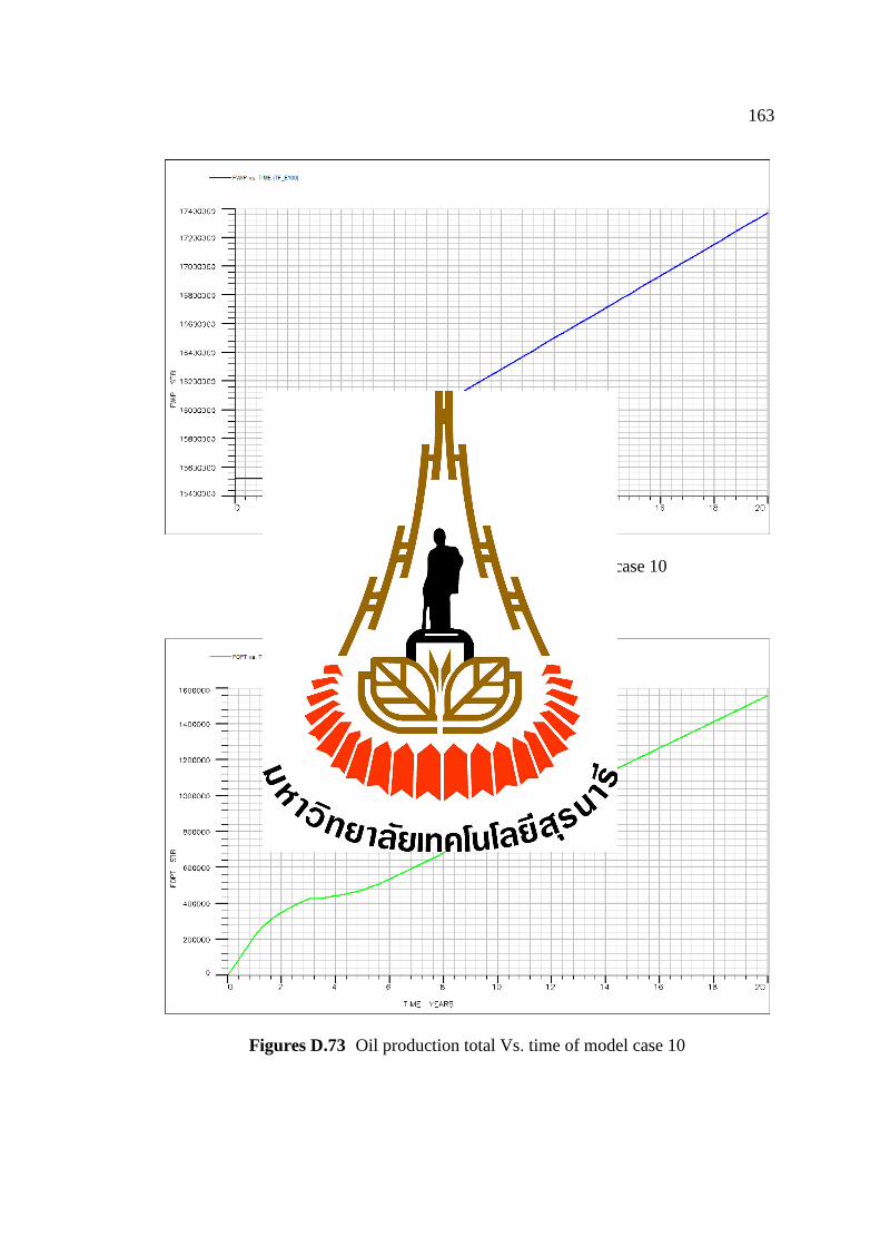
163
Figures D.72 Water in place Vs. time of model case 10
Figures D.73 Oil production total Vs. time of model case 10
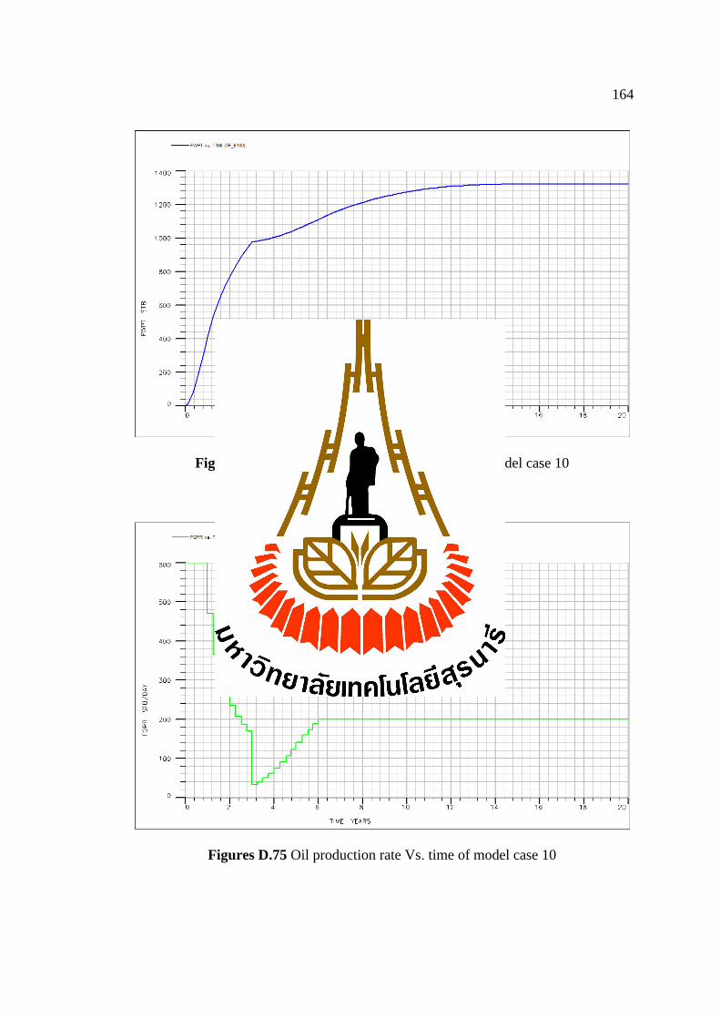
164
Figures D.74 Water production total Vs. time of model case 10
Figures D.75 Oil production rate Vs. time of model case 10

165
Figures D.76 Water production rate Vs. time of case 10
Figures D.77 Field pressure Vs. time of model case 10
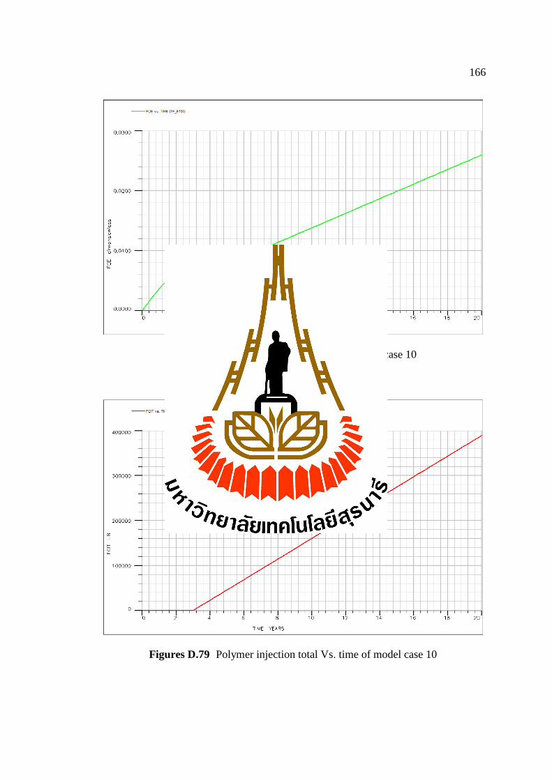
166
Figures D.78 Oil efficiency Vs. time of model case 10
Figures D.79 Polymer injection total Vs. time of model case 10
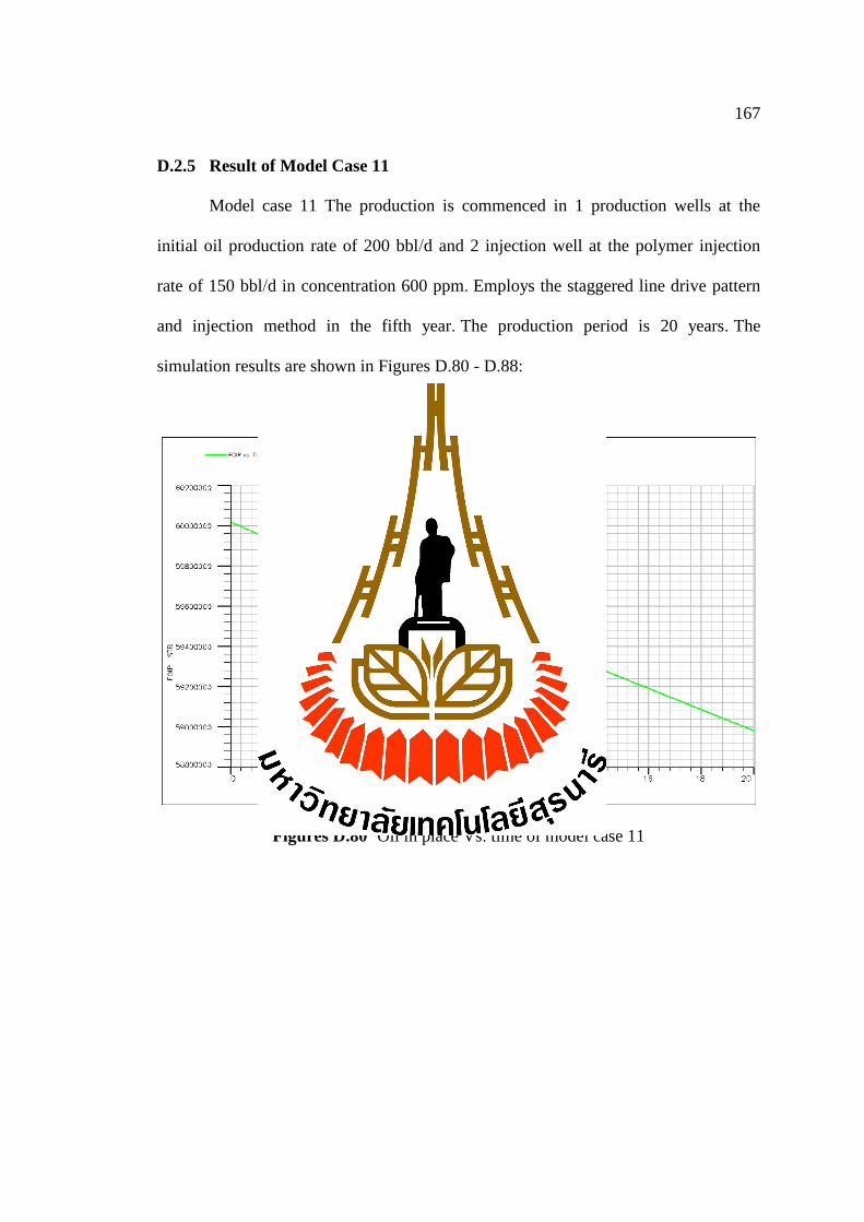
167
D.2.5 Result of Model Case 11
Model case 11 The production is commenced in 1 production wells at the
initial oil production rate of 200 bbl/d and 2 injection well at the polymer injection
rate of 150 bbl/d in concentration 600 ppm. Employs the staggered line drive pattern
and injection method in the fifth year. The production period is 20 years. The
simulation results are shown in Figures D.80 - D.88:
Figures D.80 Oil in place Vs. time of model case 11
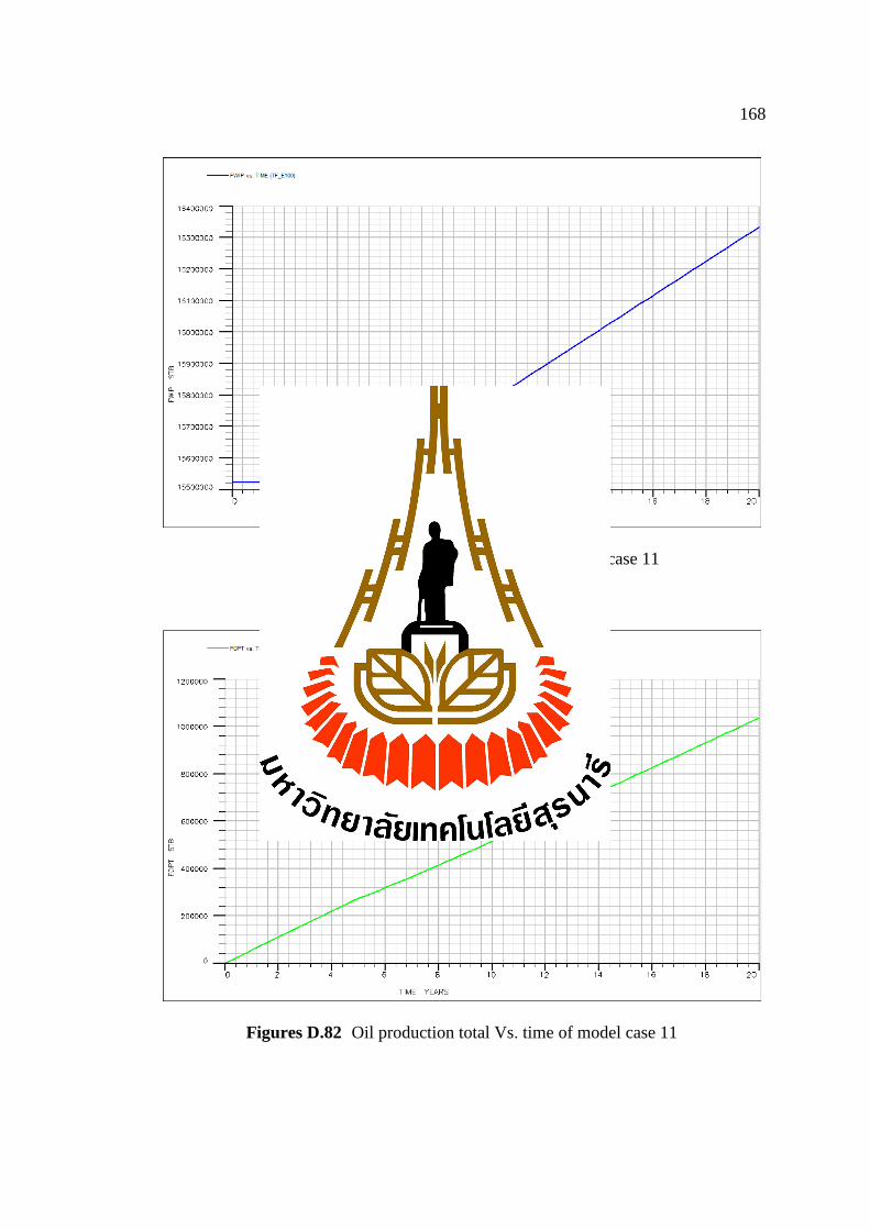
168
Figures D.81 Water in place Vs. time of model case 11
Figures D.82 Oil production total Vs. time of model case 11

169
Figures D.83 Water production total Vs. time of model case 11
Figures D.84 Oil production rate Vs. time of model case 11
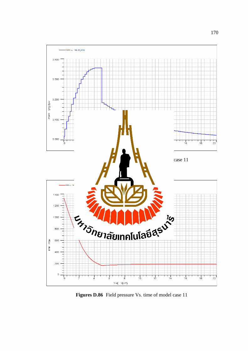
170
Figures D.85 Water production rate Vs. time of case 11
Figures D.86 Field pressure Vs. time of model case 11

171
Figures D.87 Oil efficiency Vs. time of model case 11
Figures D.88 Polymer injection total Vs. time of model case 11

172
D.2.5 Result of Model Case 12
Model case 12 The production is commenced in 1 production wells at the
initial oil production rate of 200 bbl/d and 2 injection well at the polymer injection
rate of 300 bbl/d in concentration 600 ppm. Employs the staggered line drive pattern
and injection method in the fifth year. The production period is 20 years. The
simulation results are shown in Figures D.89 - D.97:
Figures D.89 Oil in place Vs. time of model case 12
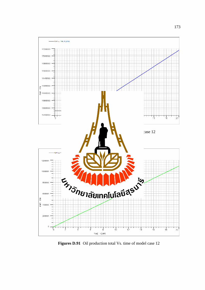
173
Figures D.90 Water in place Vs. time of model case 12
Figures D.91 Oil production total Vs. time of model case 12
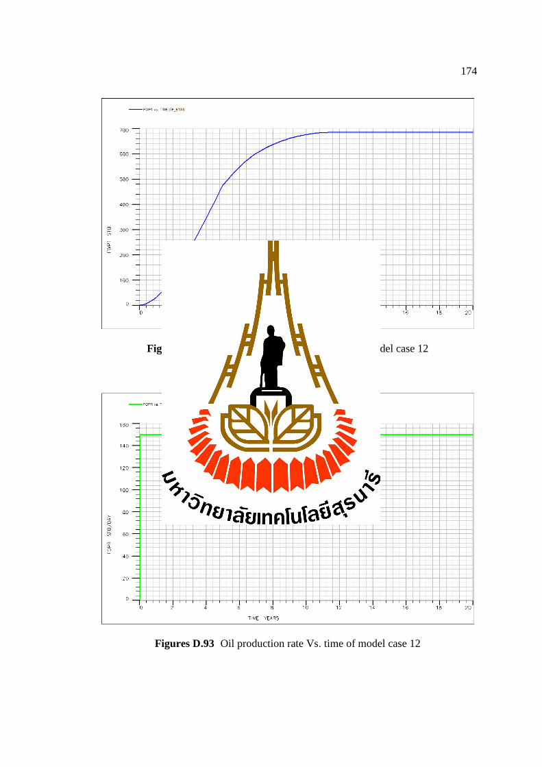
174
Figures D.92 Water production total Vs. time of model case 12
Figures D.93 Oil production rate Vs. time of model case 12
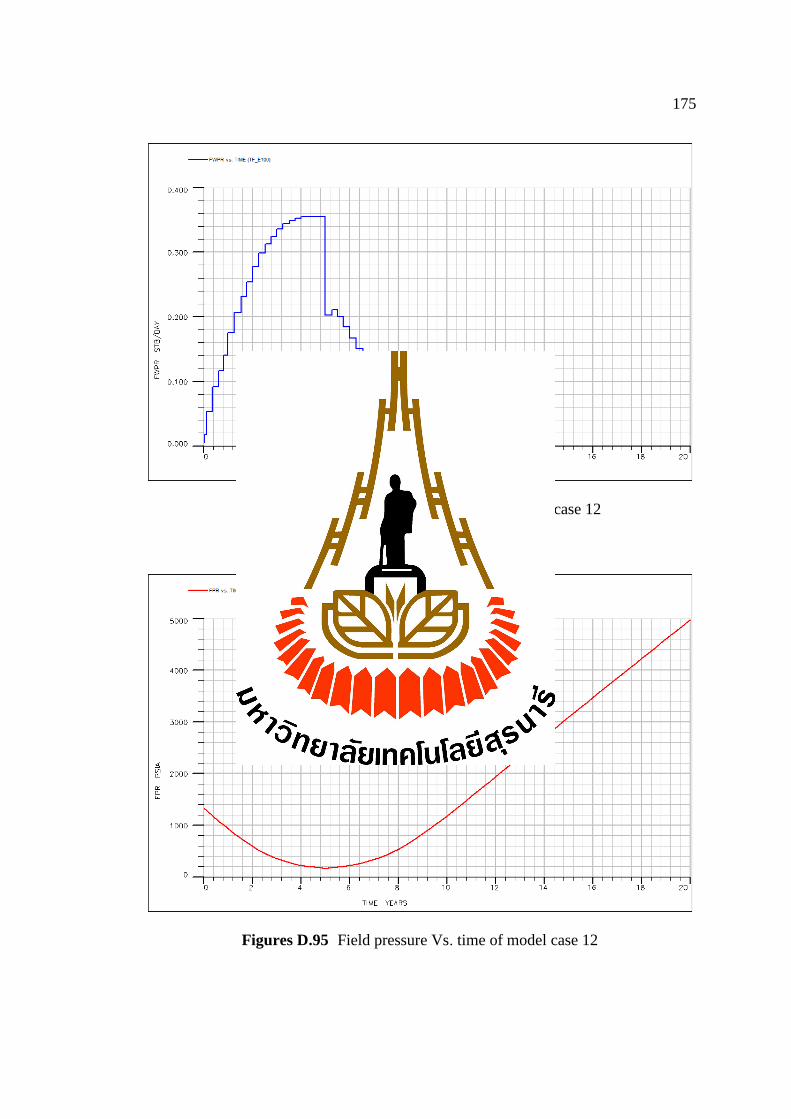
175
Figures D.94 Water production rate Vs. time of case 12
Figures D.95 Field pressure Vs. time of model case 12
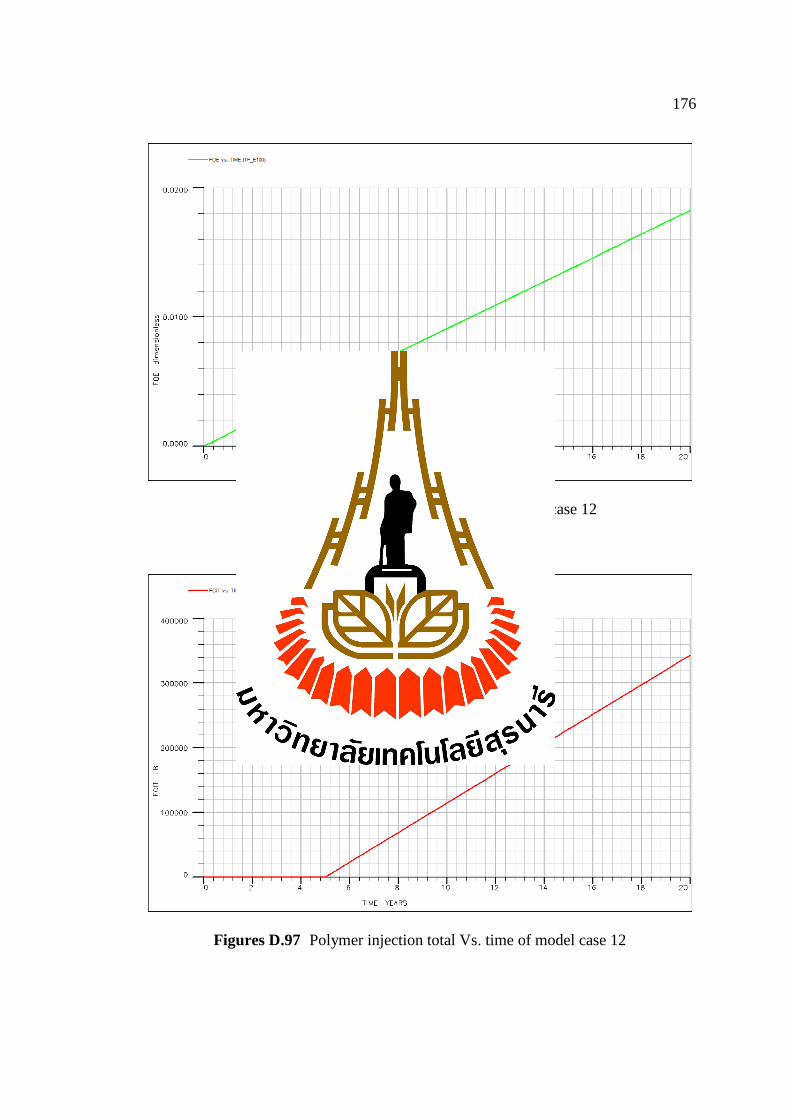
176
Figures D.96 Oil efficiency Vs. time of model case 12
Figures D.97 Polymer injection total Vs. time of model case 12
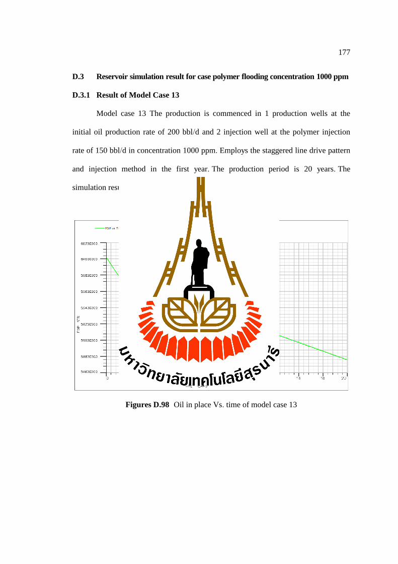
177
D.3 Reservoir simulation result for case polymer flooding concentration 1000 ppm
D.3.1 Result of Model Case 13
Model case 13 The production is commenced in 1 production wells at the
initial oil production rate of 200 bbl/d and 2 injection well at the polymer injection
rate of 150 bbl/d in concentration 1000 ppm. Employs the staggered line drive pattern
and injection method in the first year. The production period is 20 years. The
simulation results are shown in Figures D.98 - D.106:
Figures D.98 Oil in place Vs. time of model case 13
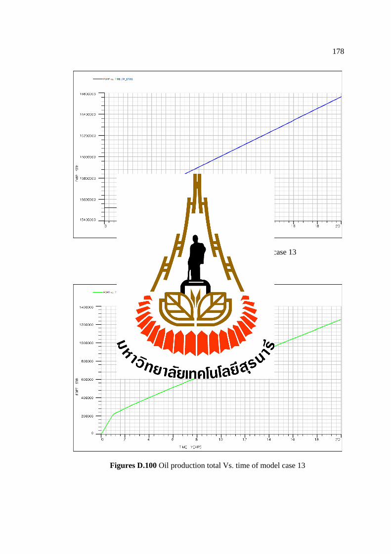
178
Figures D.99 Water in place Vs. time of model case 13
Figures D.100 Oil production total Vs. time of model case 13
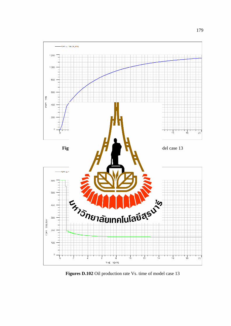
179
Figures D.101 Water production total Vs. time of model case 13
Figures D.102 Oil production rate Vs. time of model case 13
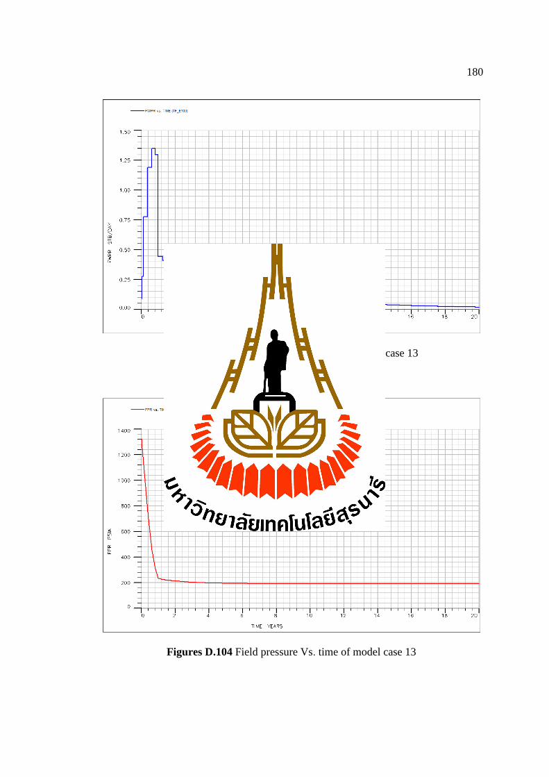
180
Figures D.103 Water production rate Vs. time of case 13
Figures D.104 Field pressure Vs. time of model case 13
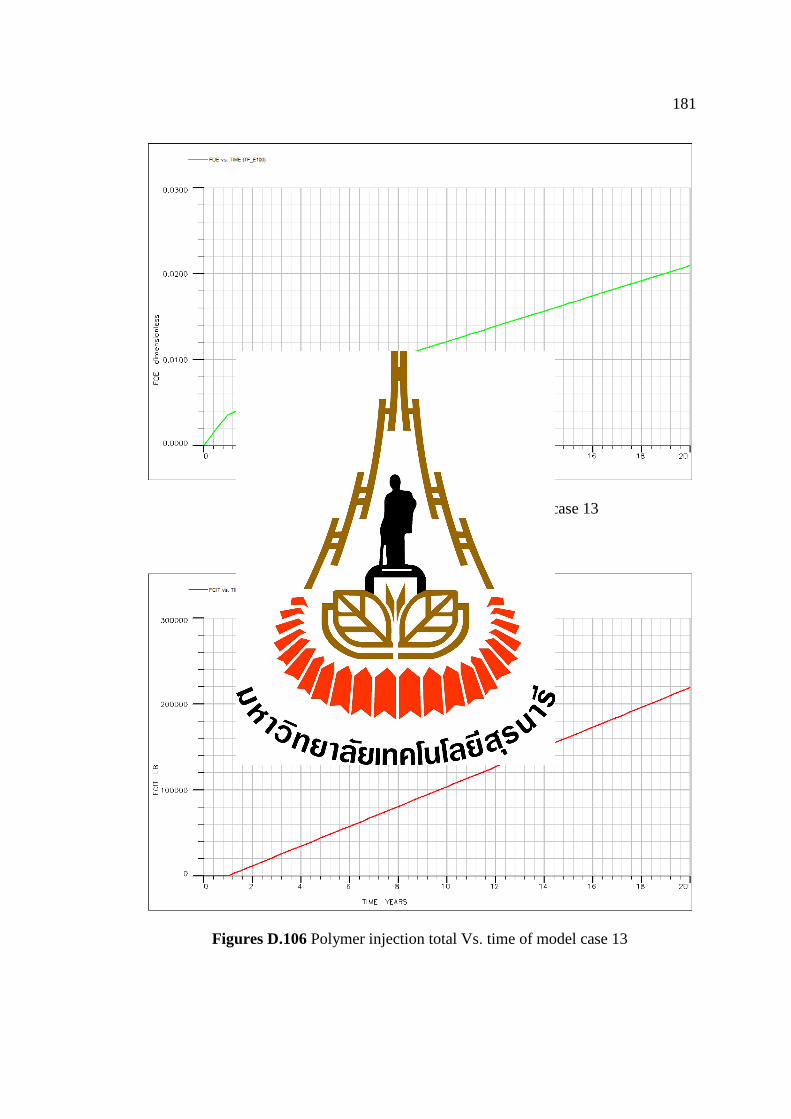
181
Figures D.105 Oil efficiency Vs. time of model case 13
Figures D.106 Polymer injection total Vs. time of model case 13

182
D.3.2 Result of Model Case 14
Model case 14 The production is commenced in 1 production wells at the
initial oil production rate of 200 bbl/d and 2 injection well at the polymer injection
rate of 300 bbl/d in concentration 1000 ppm. Employs the staggered line drive pattern
and injection method in the first year. The production period is 20 years. The
simulation results are shown in Figures D.107 - D.115:
Figures D.107 Oil in place Vs. time of model case 14
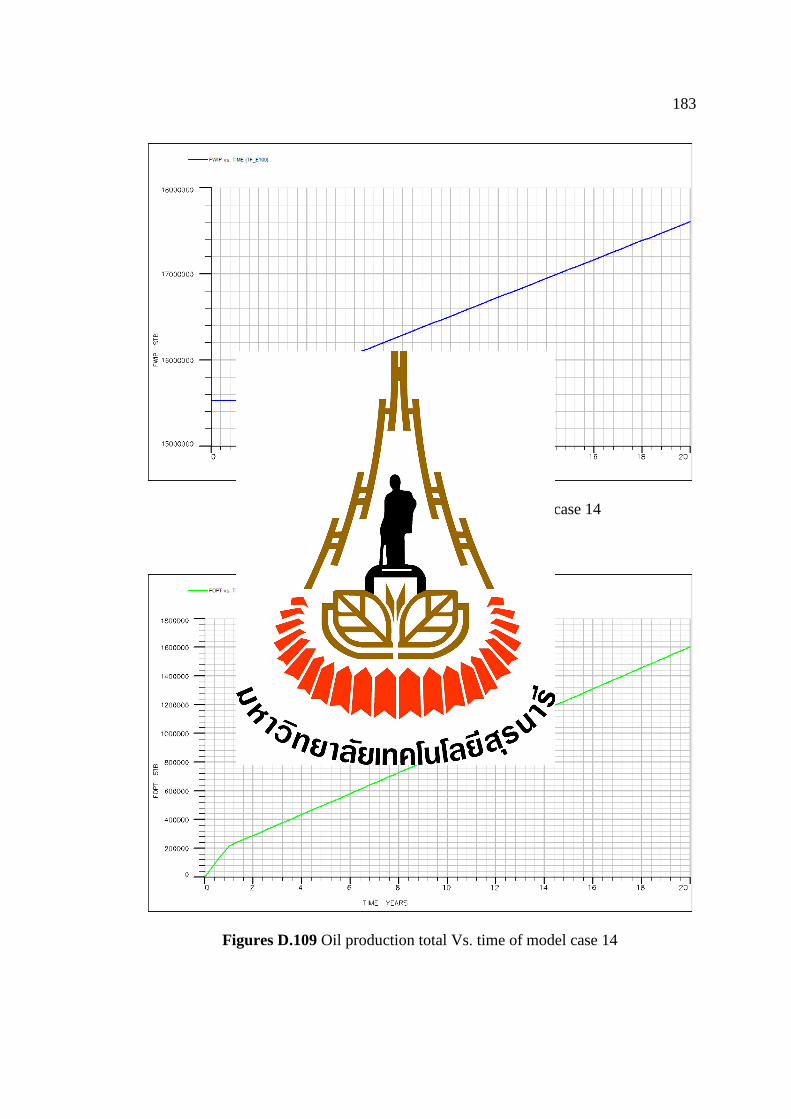
183
Figures D.108 Water in place Vs. time of model case 14
Figures D.109 Oil production total Vs. time of model case 14
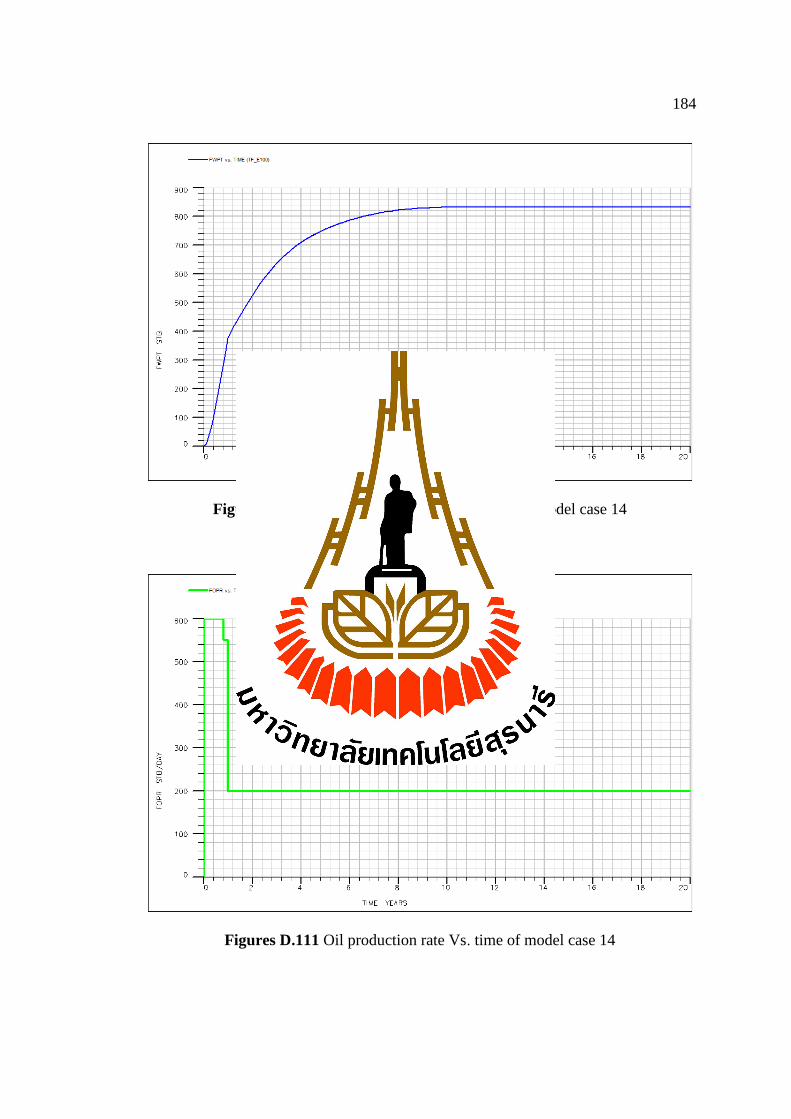
184
Figures D.110 Water production total Vs. time of model case 14
Figures D.111 Oil production rate Vs. time of model case 14

185
Figures D.112 Water production rate Vs. time of case 14
Figures D.113 Field pressure Vs. time of model case 14
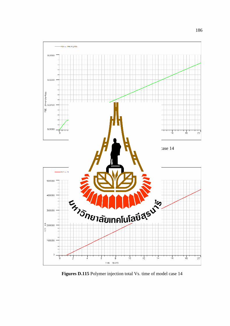
186
Figures D.114 Oil efficiency Vs. time of model case 14
Figures D.115 Polymer injection total Vs. time of model case 14

187
D.3.3 Result of Model Case 15
Model case 15 The production is commenced in 1 production wells at the
initial oil production rate of 200 bbl/d and 2 injection well at the polymer injection
rate of 150 bbl/d in concentration 1000 ppm. Employs the staggered line drive pattern
and injection method in the third year. The production period is 20 years. The
simulation results are shown in Figures D.116 - D.124:
Figures D.116 Oil in place Vs. time of model case 15
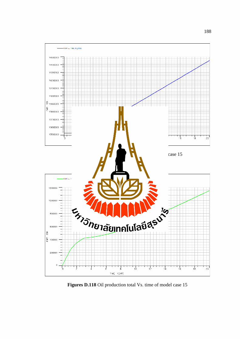
188
Figures D.117 Water in place Vs. time of model case 15
Figures D.118 Oil production total Vs. time of model case 15
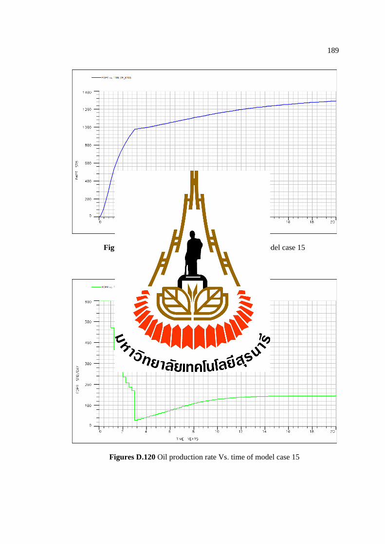
189
Figures D.119 Water production total Vs. time of model case 15
Figures D.120 Oil production rate Vs. time of model case 15
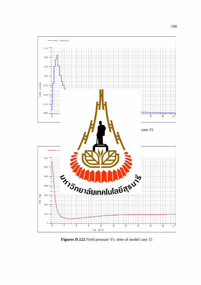
190
Figures D.121 Water production rate Vs. time of case 15
Figures D.122 Field pressure Vs. time of model case 15
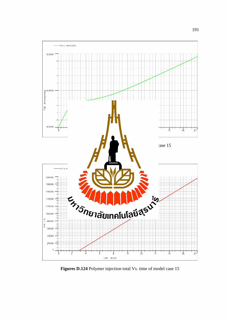
191
Figures D.123 Oil efficiency Vs. time of model case 15
Figures D.124 Polymer injection total Vs. time of model case 15
192
D.3.4 Result of Model Case 16
Model case 16 The production is commenced in 1 production wells at the
initial oil production rate of 200 bbl/d and 2 injection well at the polymer injection
rate of 300 bbl/d in concentration 1000 ppm. Employs the staggered line drive pattern
and injection method in the third year. The production period is 20 years. The
simulation results are shown in Figures D.125 - D.133:
Figures D.125 Oil in place Vs. time of model case 16
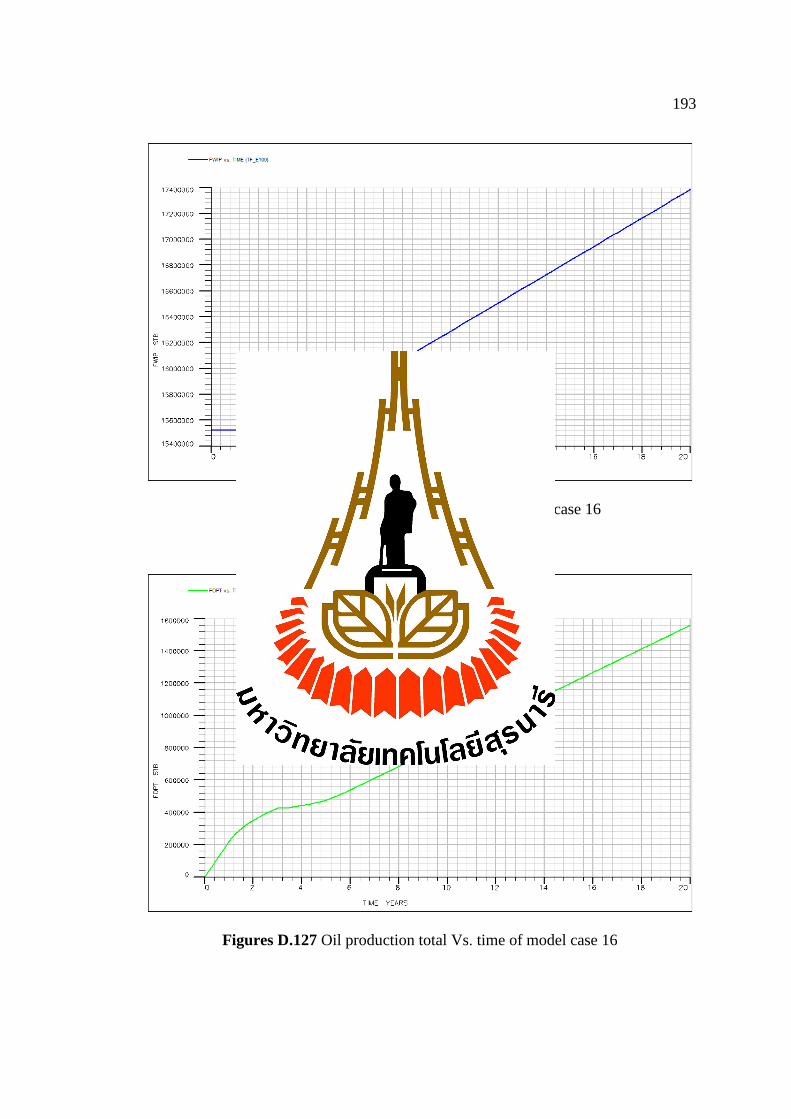
193
Figures D.126 Water in place Vs. time of model case 16
Figures D.127 Oil production total Vs. time of model case 16
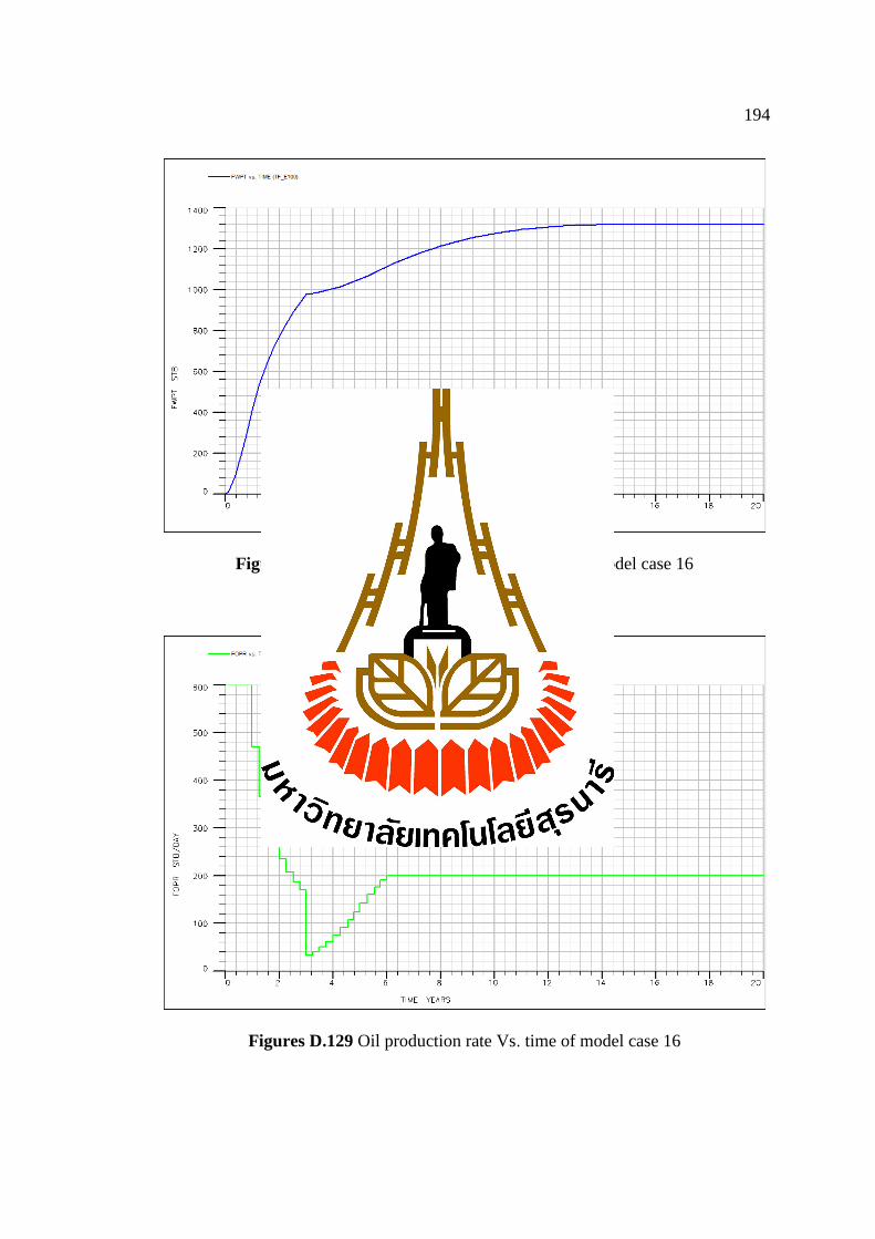
194
Figures D.128 Water production total Vs. time of model case 16
Figures D.129 Oil production rate Vs. time of model case 16
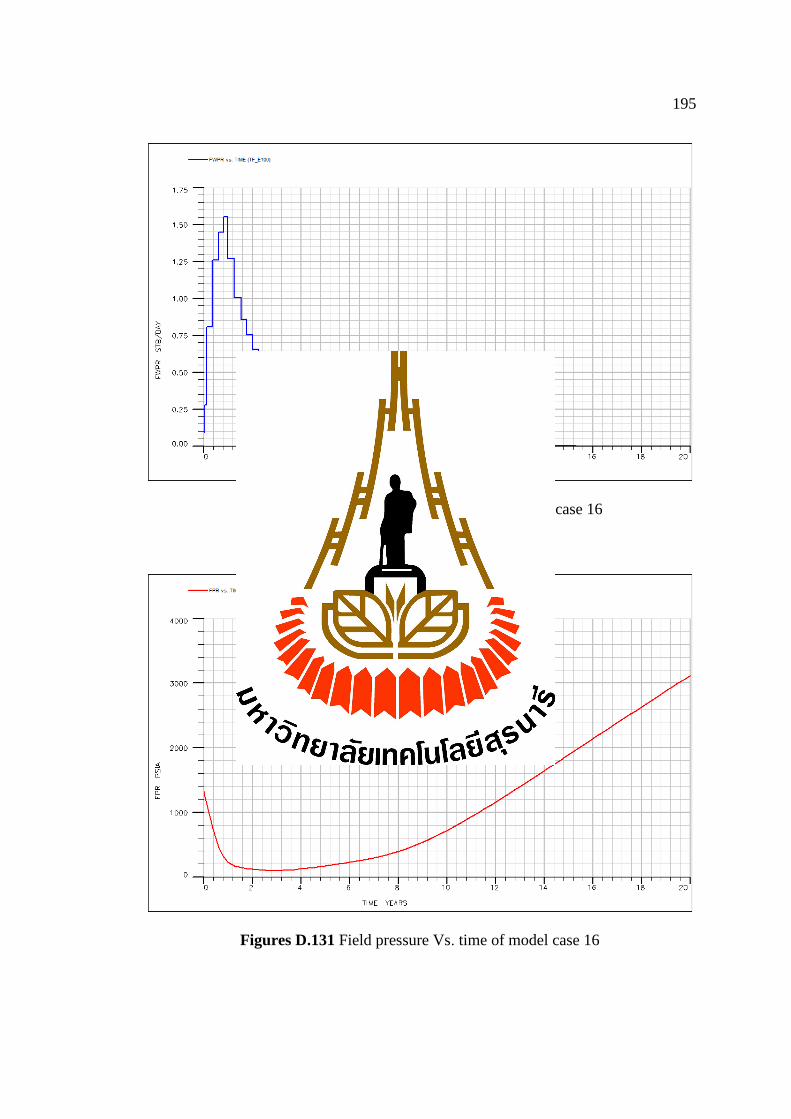
195
Figures D.130 Water production rate Vs. time of case 16
Figures D.131 Field pressure Vs. time of model case 16

196
Figures D.132 Oil efficiency Vs. time of model case 16
Figures D.133 Polymer injection total Vs. time of model case 16
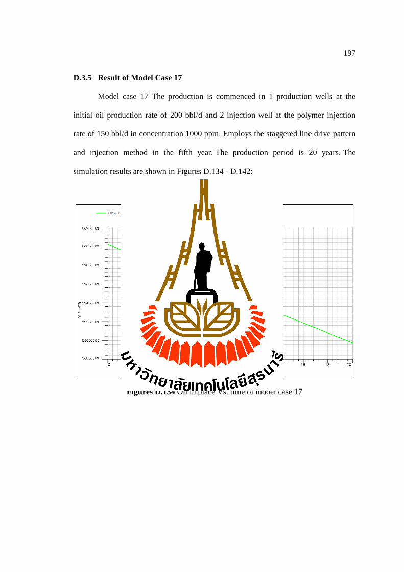
197
D.3.5 Result of Model Case 17
Model case 17 The production is commenced in 1 production wells at the
initial oil production rate of 200 bbl/d and 2 injection well at the polymer injection
rate of 150 bbl/d in concentration 1000 ppm. Employs the staggered line drive pattern
and injection method in the fifth year. The production period is 20 years. The
simulation results are shown in Figures D.134 - D.142:
Figures D.134 Oil in place Vs. time of model case 17
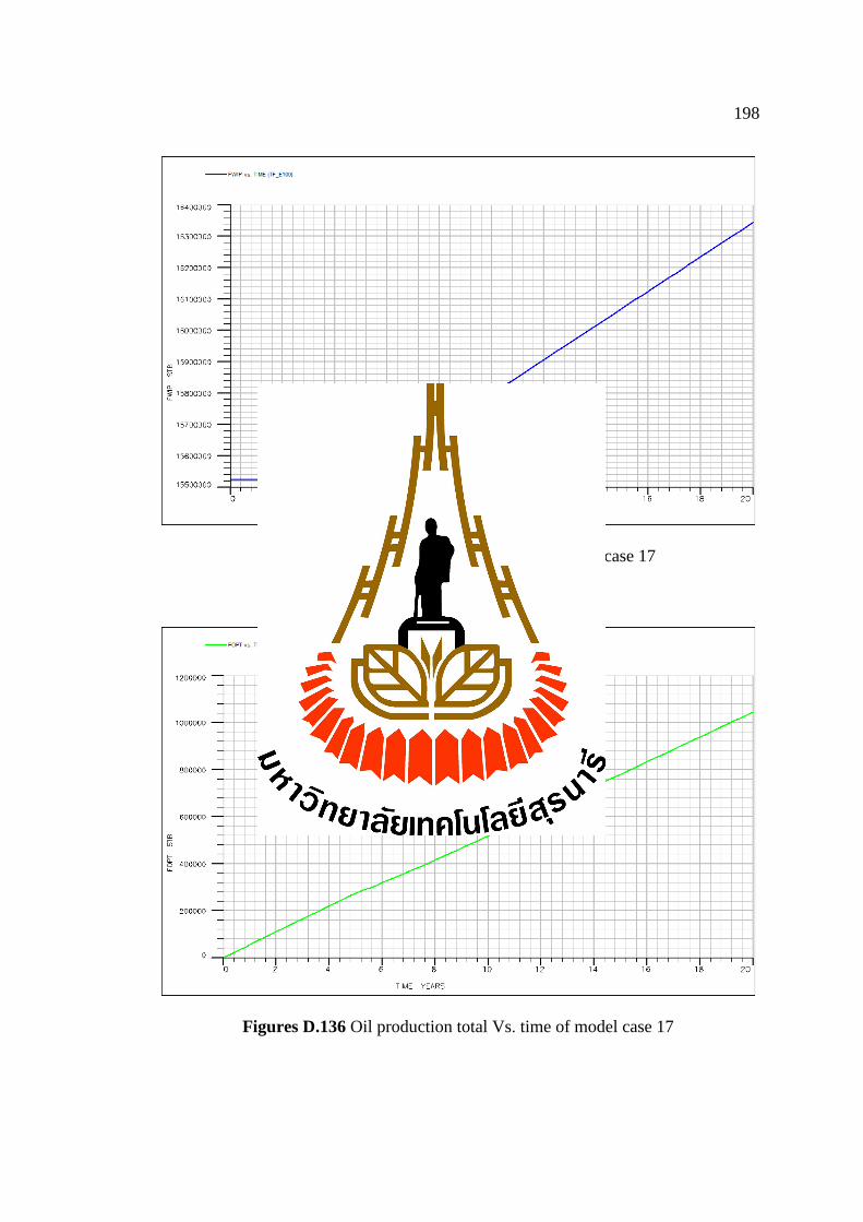
198
Figures D.135 Water in place Vs. time of model case 17
Figures D.136 Oil production total Vs. time of model case 17
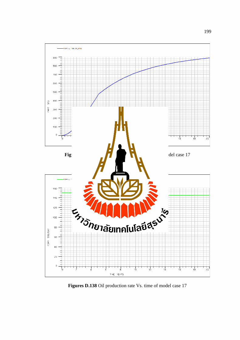
199
Figures D.137 Water production total Vs. time of model case 17
Figures D.138 Oil production rate Vs. time of model case 17
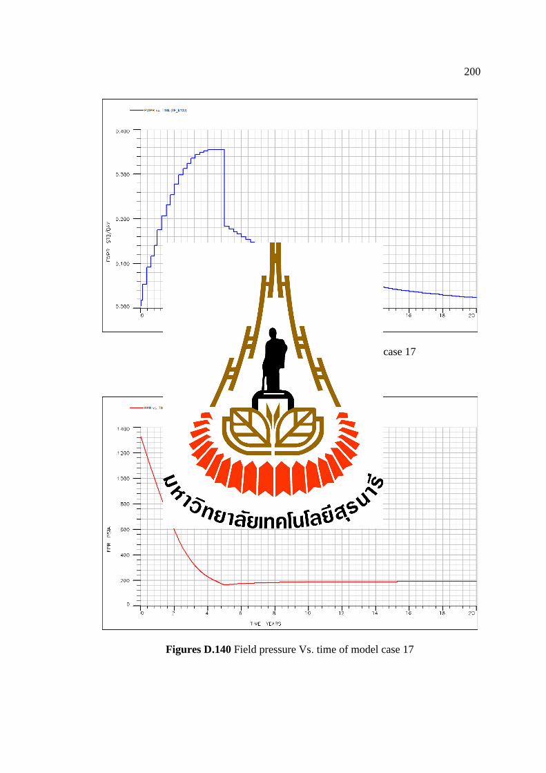
200
Figures D.139 Water production rate Vs. time of case 17
Figures D.140 Field pressure Vs. time of model case 17
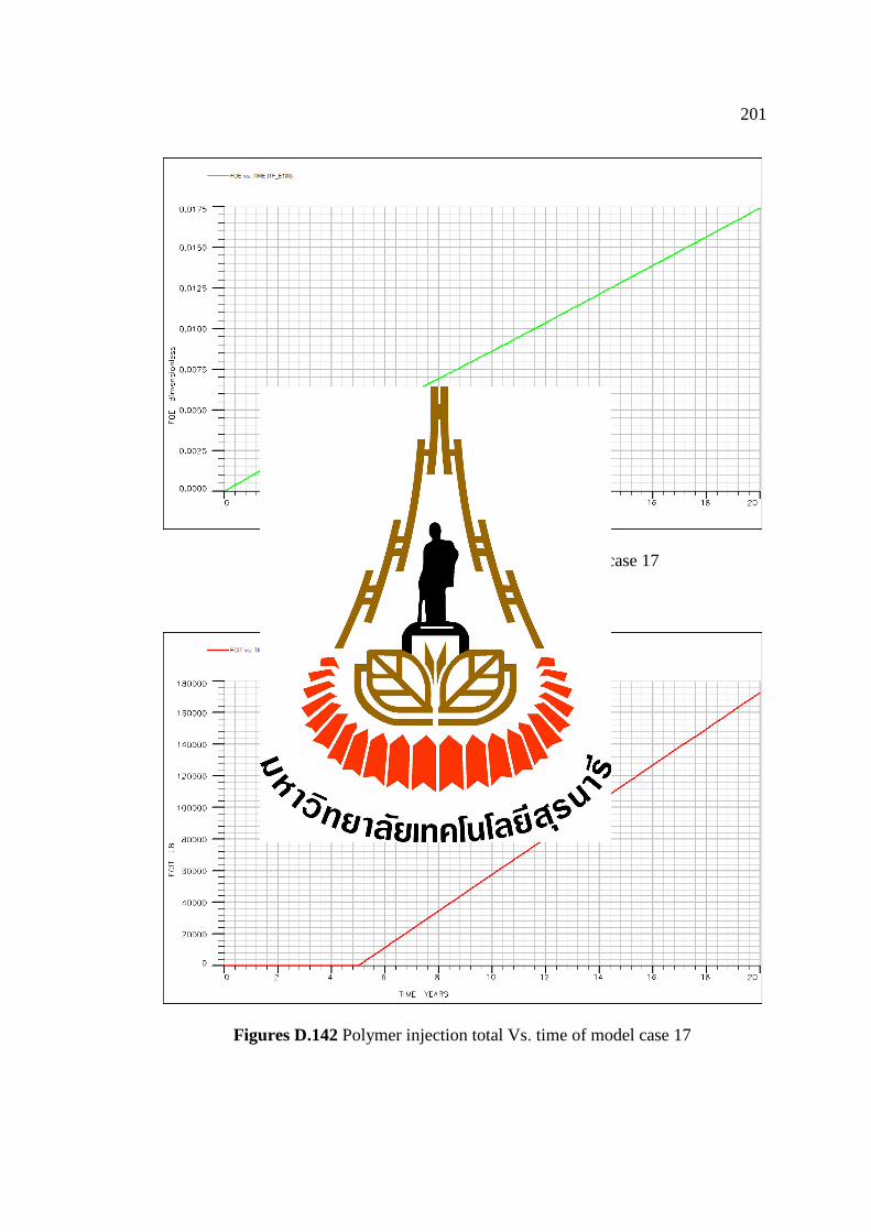
201
Figures D.141 Oil efficiency Vs. time of model case 17
Figures D.142 Polymer injection total Vs. time of model case 17

202
D.3.6 Result of Model Case 18
Model case 18 The production is commenced in 1 production wells at the
initial oil production rate of 200 bbl/d and 2 injection well at the polymer injection
rate of 300 bbl/d in concentration 1000 ppm. Employs the staggered line drive pattern
and injection method in the fifth year. The production period is 20 years. The
simulation results are shown in Figures D.143 - D.151:
Figures D.143 Oil in place Vs. time of model case 18

203
Figures D.144 Water in place Vs. time of model case 18
Figures D.145 Oil production total Vs. time of model case 18
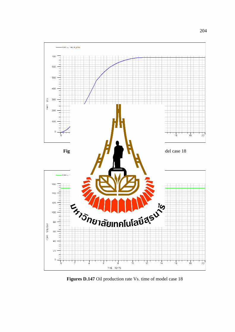
204
Figures D.146 Water production total Vs. time of model case 18
Figures D.147 Oil production rate Vs. time of model case 18

205
Figures D.148 Water production rate Vs. time of case 18
Figures D.149 Field pressure Vs. time of model case 18
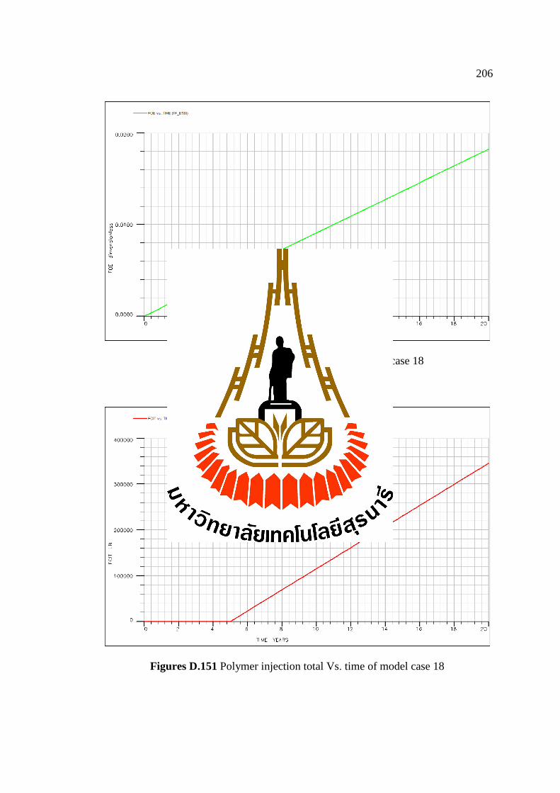
206
Figures D.150 Oil efficiency Vs. time of model case 18
Figures D.151 Polymer injection total Vs. time of model case 18

207
D.4 Reservoir simulation result for case polymer flooding concentration 1500 ppm
D.4.1 Result of Model Case 19
Model case 19 The production is commenced in 1 production wells at the
initial oil production rate of 200 bbl/d and 2 injection well at the polymer injection
rate of 150 bbl/d in concentration 1500 ppm. Employs the staggered line drive pattern
and injection method in the first year. The production period is 20 years. The
simulation results are shown in Figures D.152 - D.160:
Figures D.152 Oil in place Vs. time of model case 19
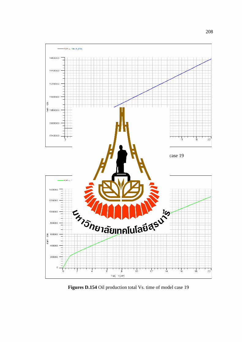
208
Figures D.153 Water in place Vs. time of model case 19
Figures D.154 Oil production total Vs. time of model case 19
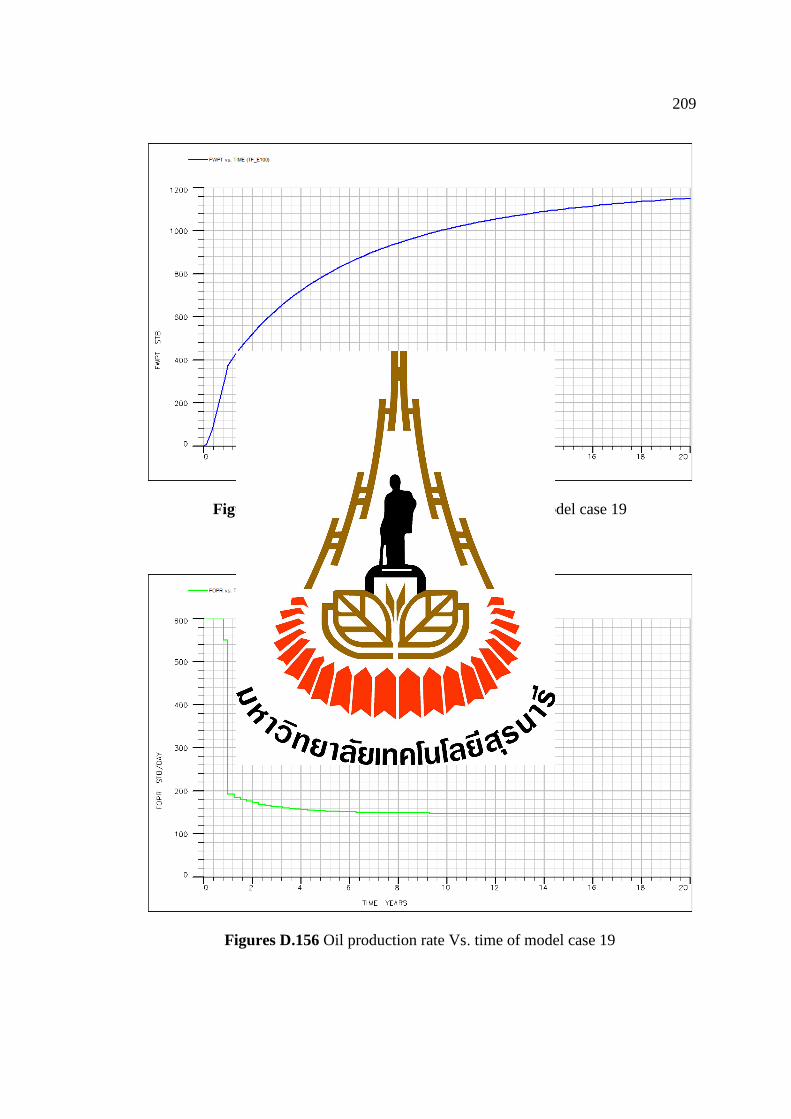
209
Figures D.155 Water production total Vs. time of model case 19
Figures D.156 Oil production rate Vs. time of model case 19
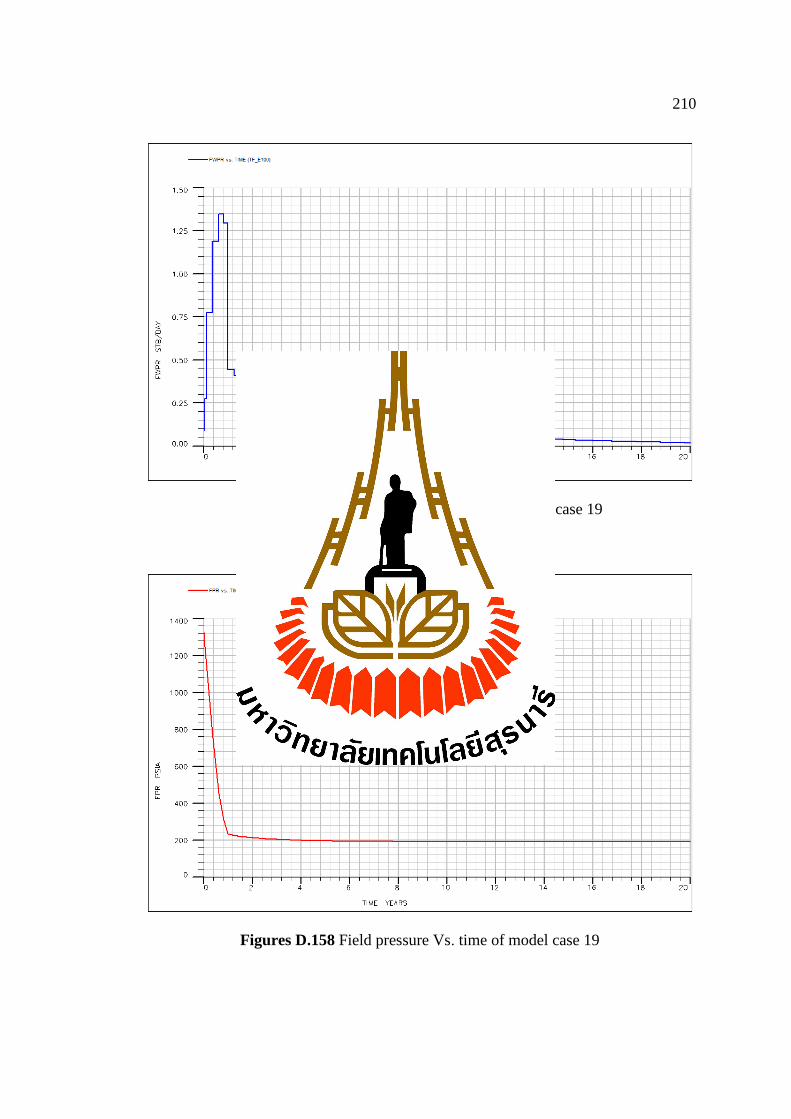
210
Figures D.157 Water production rate Vs. time of case 19
Figures D.158 Field pressure Vs. time of model case 19

211
Figures D.159 Oil efficiency Vs. time of model case 19
Figures D.160 Polymer injection total Vs. time of model case 19
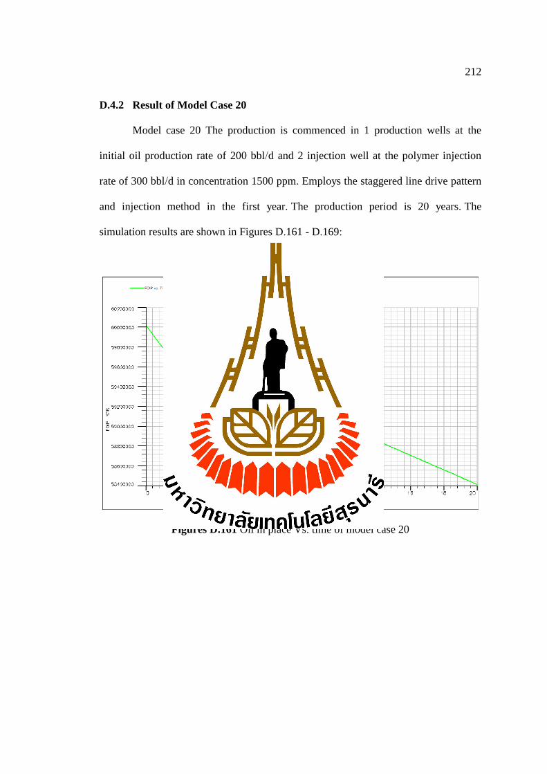
212
D.4.2 Result of Model Case 20
Model case 20 The production is commenced in 1 production wells at the
initial oil production rate of 200 bbl/d and 2 injection well at the polymer injection
rate of 300 bbl/d in concentration 1500 ppm. Employs the staggered line drive pattern
and injection method in the first year. The production period is 20 years. The
simulation results are shown in Figures D.161 - D.169:
Figures D.161 Oil in place Vs. time of model case 20
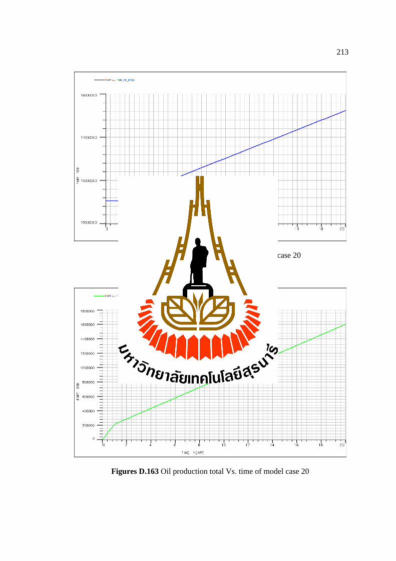
213
Figures D.162 Water in place Vs. time of model case 20
Figures D.163 Oil production total Vs. time of model case 20
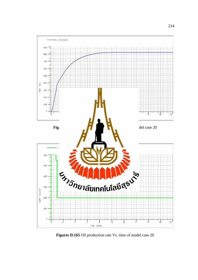
214
Figures D.164 Water production total Vs. time of model case 20
Figures D.165 Oil production rate Vs. time of model case 20
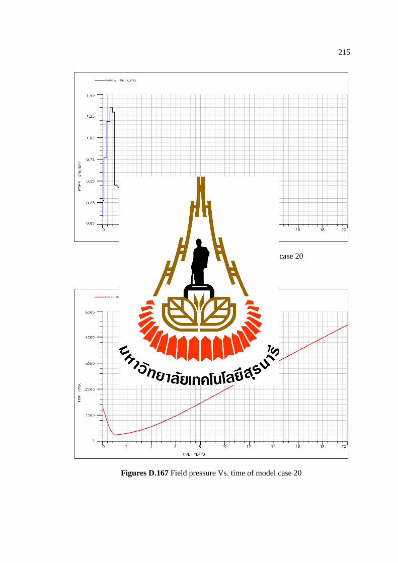
215
Figures D.166 Water production rate Vs. time of case 20
Figures D.167 Field pressure Vs. time of model case 20
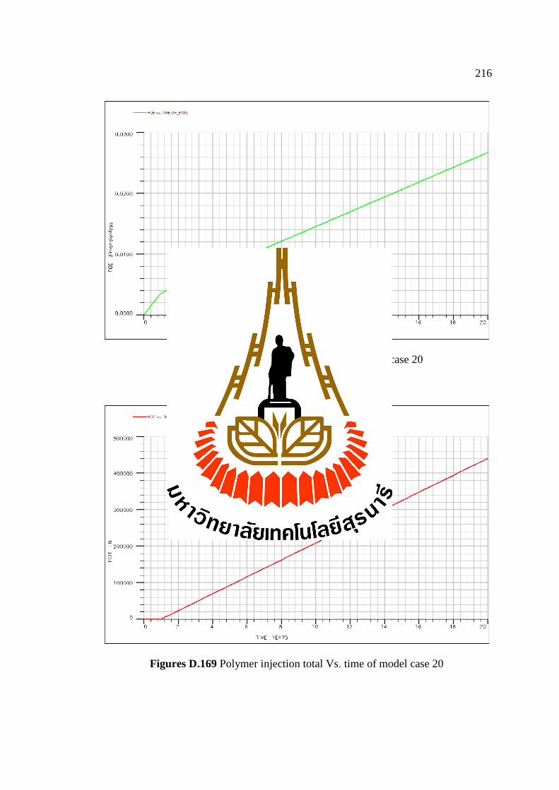
216
Figures D.168 Oil efficiency Vs. time of model case 20
Figures D.169 Polymer injection total Vs. time of model case 20

217
D.4.3 Result of Model Case 21
Model case 21 The production is commenced in 1 production wells at the
initial oil production rate of 200 bbl/d and 2 injection well at the polymer injection
rate of 150 bbl/d in concentration 1500 ppm. Employs the staggered line drive pattern
and injection method in the third year. The production period is 20 years. The
simulation results are shown in Figures D.170 - D.178:
Figures D.170 Oil in place Vs. time of model case 21
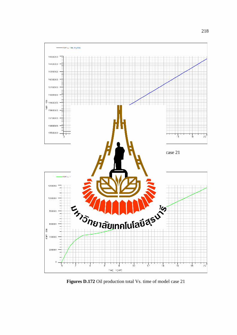
218
Figures D.171 Water in place Vs. time of model case 21
Figures D.172 Oil production total Vs. time of model case 21
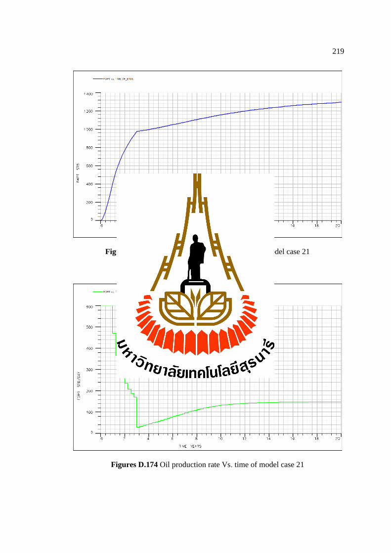
219
Figures D.173 Water production total Vs. time of model case 21
Figures D.174 Oil production rate Vs. time of model case 21
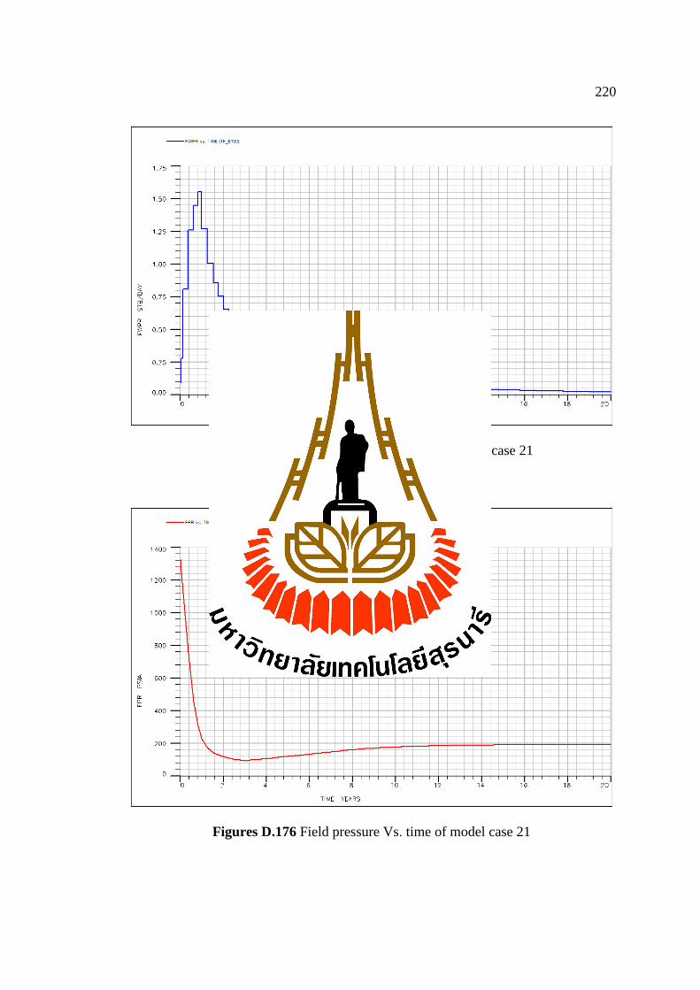
220
Figures D.175 Water production rate Vs. time of case 21
Figures D.176 Field pressure Vs. time of model case 21
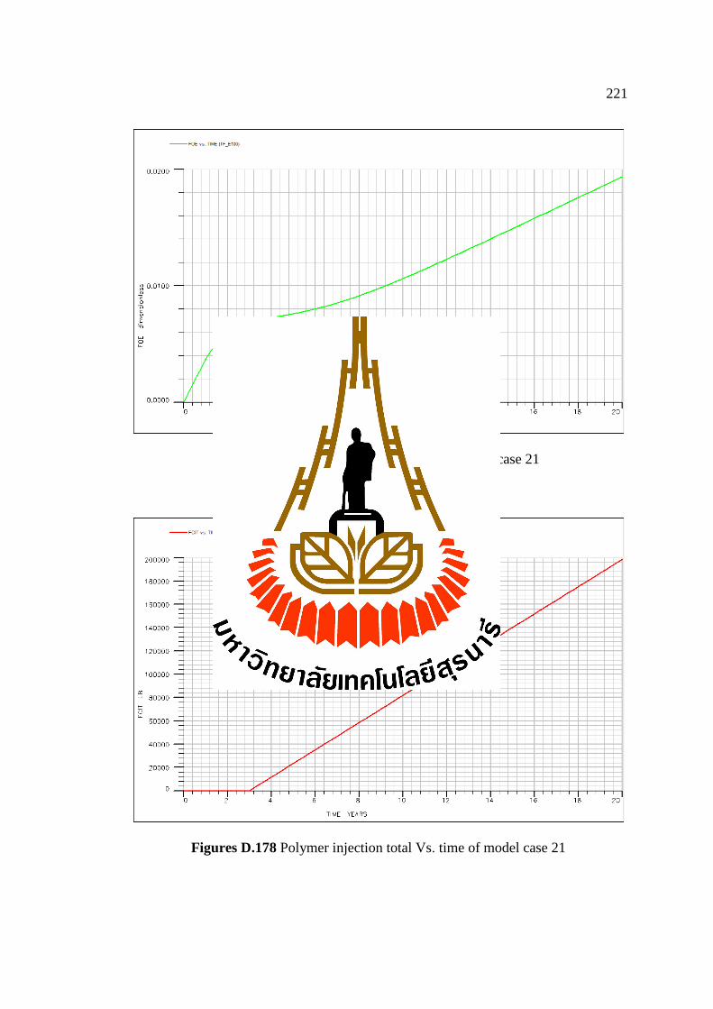
221
Figures D.177 Oil efficiency Vs. time of model case 21
Figures D.178 Polymer injection total Vs. time of model case 21
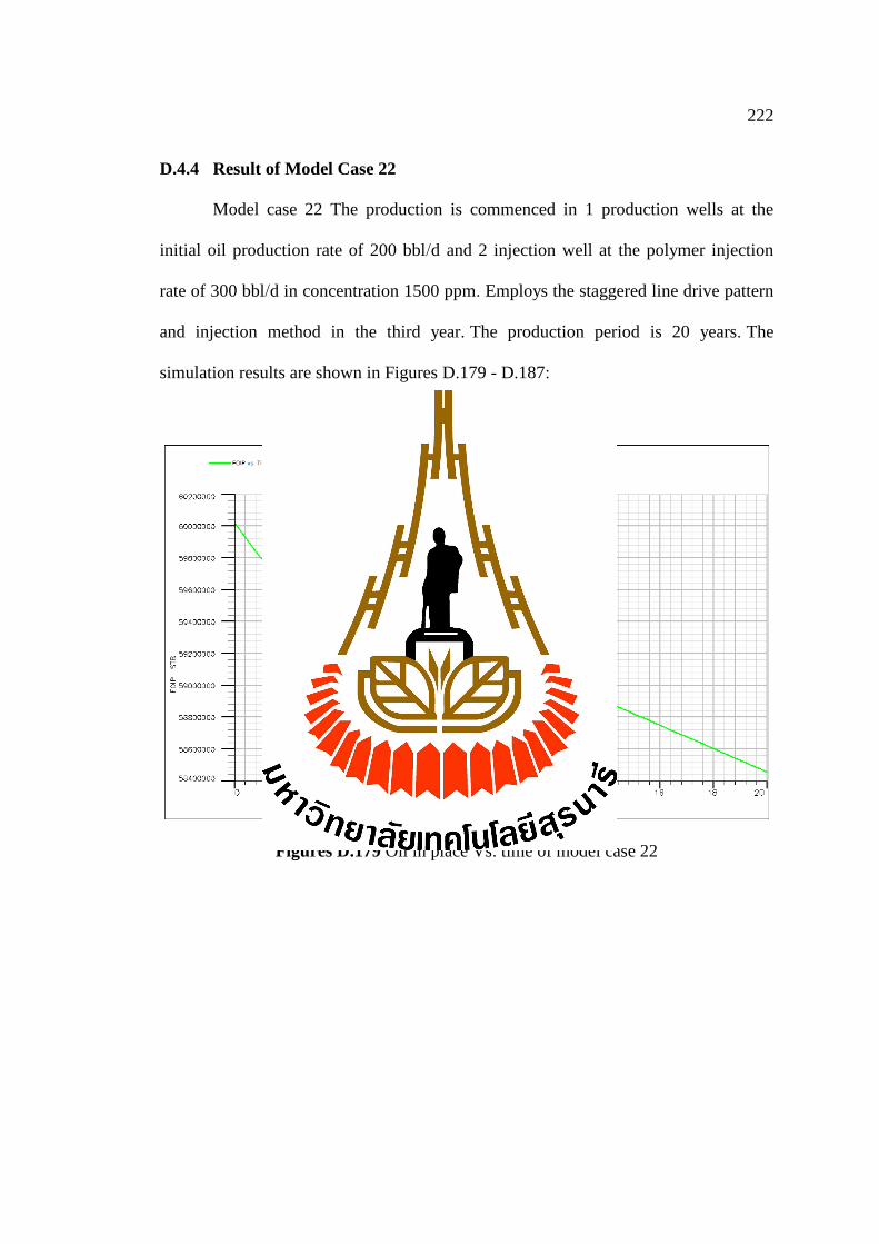
222
D.4.4 Result of Model Case 22
Model case 22 The production is commenced in 1 production wells at the
initial oil production rate of 200 bbl/d and 2 injection well at the polymer injection
rate of 300 bbl/d in concentration 1500 ppm. Employs the staggered line drive pattern
and injection method in the third year. The production period is 20 years. The
simulation results are shown in Figures D.179 - D.187:
Figures D.179 Oil in place Vs. time of model case 22

223
Figures D.180 Water in place Vs. time of model case 22
Figures D.181 Oil production total Vs. time of model case 22
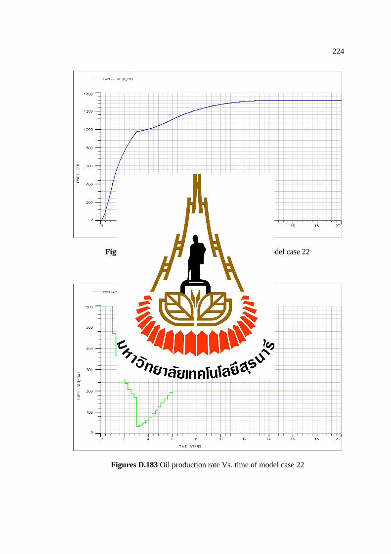
224
Figures D.182 Water production total Vs. time of model case 22
Figures D.183 Oil production rate Vs. time of model case 22
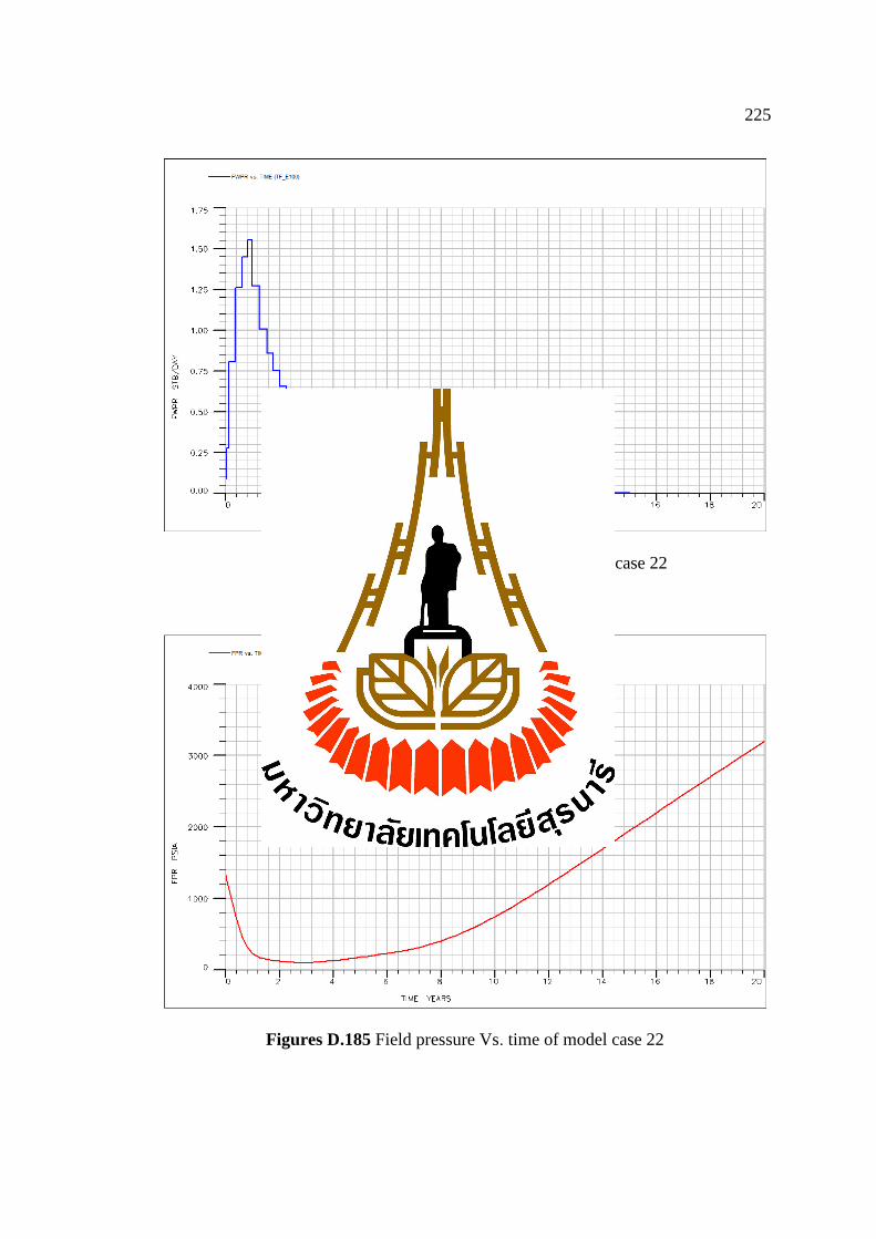
225
Figures D.184 Water production rate Vs. time of case 22
Figures D.185 Field pressure Vs. time of model case 22

226
Figures D.186 Oil efficiency Vs. time of model case 22
Figures D.187 Polymer injection total Vs. time of model case 22

227
D.4.5 Result of Model Case 23
Model case 23 The production is commenced in 1 production wells at the
initial oil production rate of 200 bbl/d and 2 injection well at the polymer injection
rate of 150 bbl/d in concentration 1500 ppm. Employs the staggered line drive pattern
and injection method in the fifth year. The production period is 20 years. The
simulation results are shown in Figures D.188 - D.196:
Figures D.188 Oil in place Vs. time of model case 23
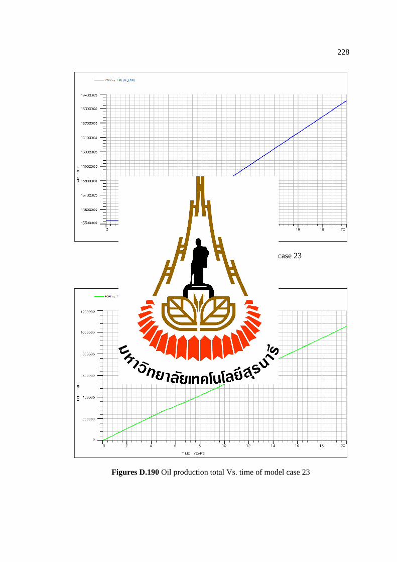
228
Figures D.189 Water in place Vs. time of model case 23
Figures D.190 Oil production total Vs. time of model case 23
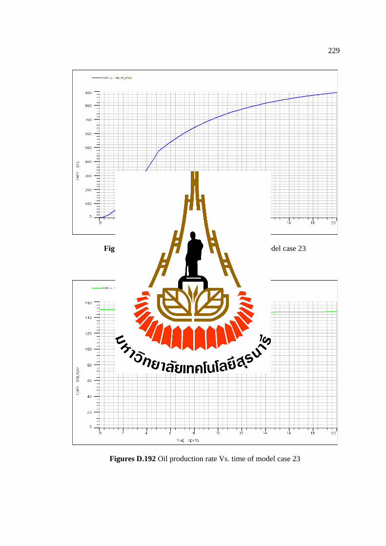
229
Figures D.191 Water production total Vs. time of model case 23
Figures D.192 Oil production rate Vs. time of model case 23
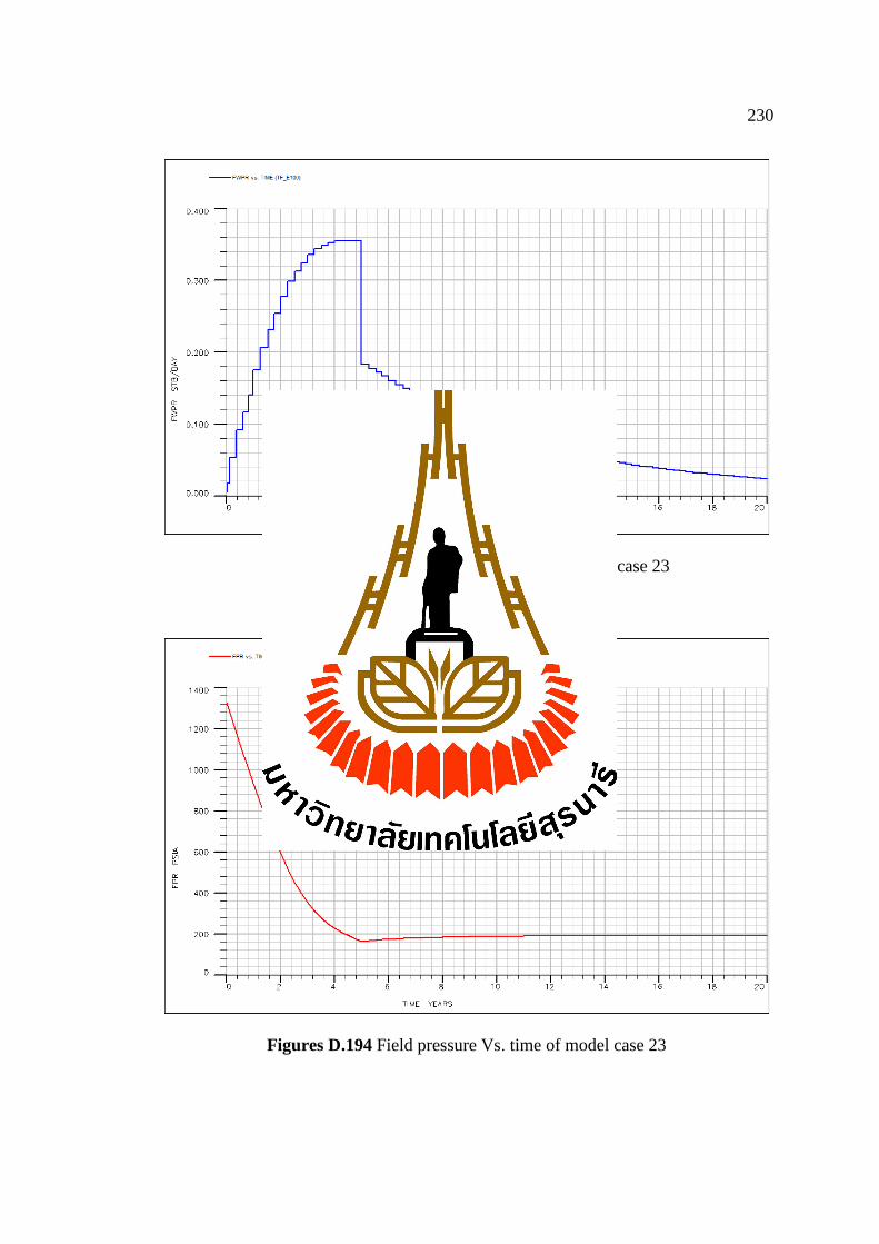
230
Figures D.193 Water production rate Vs. time of case 23
Figures D.194 Field pressure Vs. time of model case 23
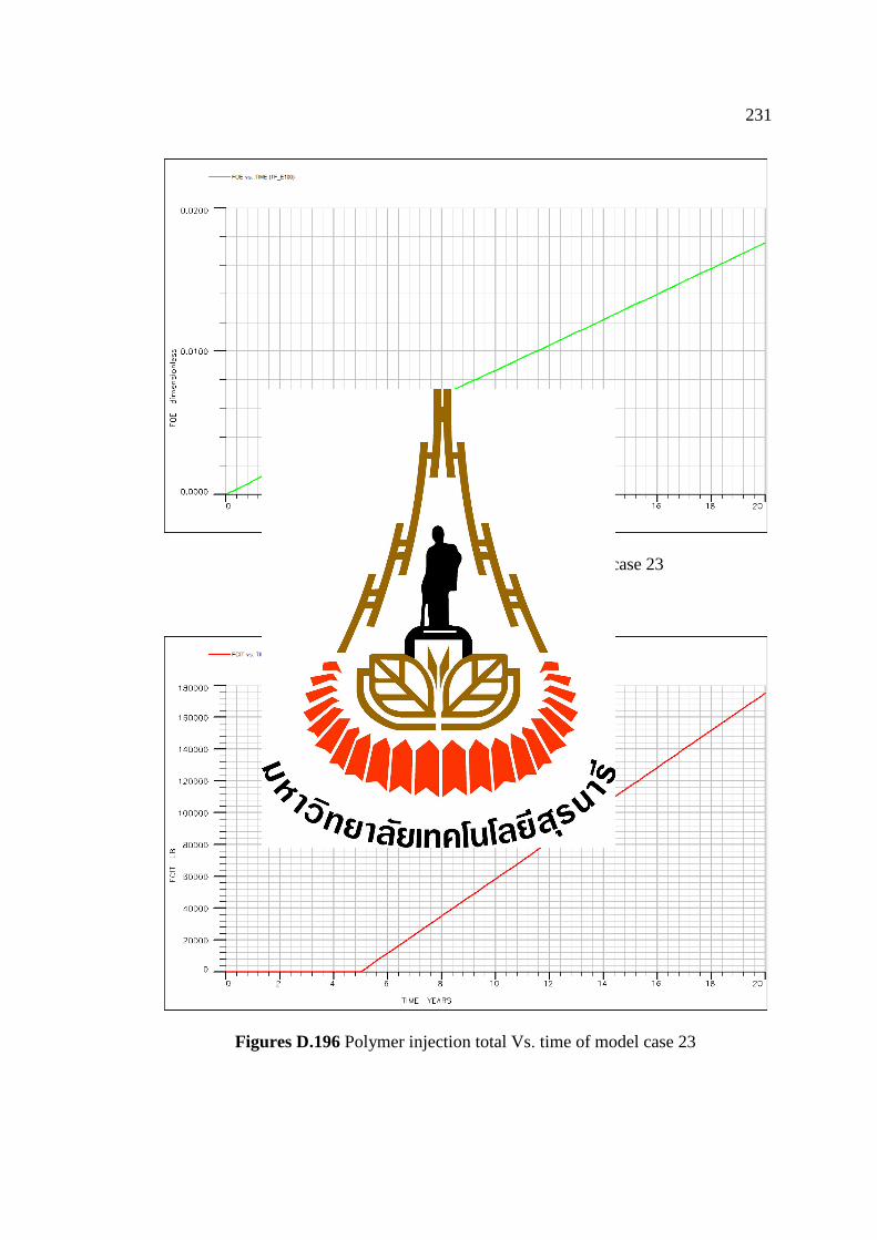
231
Figures D.195 Oil efficiency Vs. time of model case 23
Figures D.196 Polymer injection total Vs. time of model case 23

232
D.4.6 Result of Model Case 24
Model case 24 The production is commenced in 1 production wells at the
initial oil production rate of 200 bbl/d and 2 injection well at the polymer injection
rate of 300 bbl/d in concentration 1500 ppm. Employs the staggered line drive pattern
and injection method in the fifth year. The production period is 20 years. The
simulation results are shown in Figures D.197 - D.205:
Figures D.197 Oil in place Vs. time of model case 24
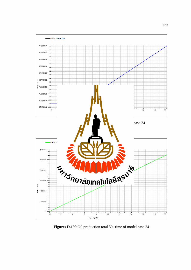
233
Figures D.198 Water in place Vs. time of model case 24
Figures D.199 Oil production total Vs. time of model case 24
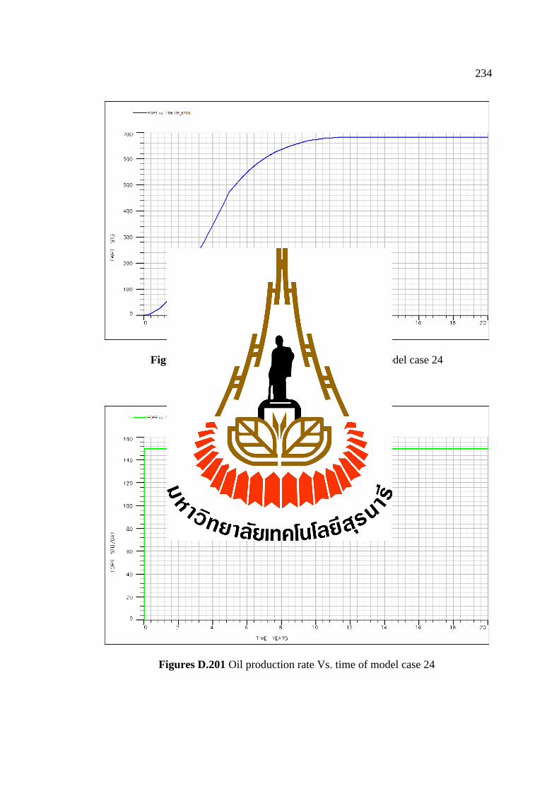
234
Figures D.200 Water production total Vs. time of model case 24
Figures D.201 Oil production rate Vs. time of model case 24

235
Figures D.202 Water production rate Vs. time of case 24
Figures D.203 Field pressure Vs. time of model case 24
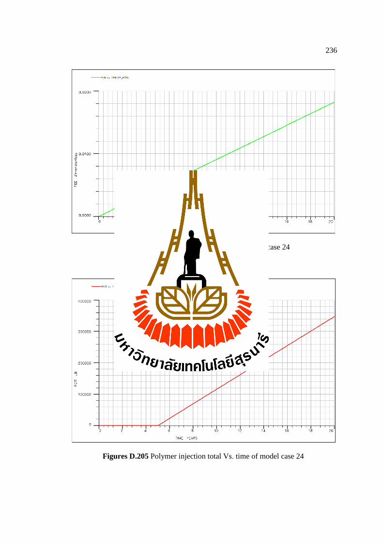
236
Figures D.204 Oil efficiency Vs. time of model case 24
Figures D.205 Polymer injection total Vs. time of model case 24

BIOGRAPHY
Mr. Suchet Nillaphan was born on the 20th January 1989 in Saraburi.
Graduated from Pibul Wittayalai School in 2007, he continued to pursue a bachelor's
degree at Suranaree University of Technology (SUT). In 2012, he earned his degree in
the School of Geotechnology.
From 2012-2017, he has studied for a master's degree in the School of
Geotechnology, Institute of Engineering at Suranaree University of Technology with
the major in Petorleum Engineering.


