Conditional value at risk and related linear programming models for portfolio optimization

Report of the Institute of Controland Computation Engineering

Warsaw University of Technology

Conditional Value at Risk and Related Linear ProgrammingModels for Portfolio Optimization

Renata Mansini, Włodzimierz Ogryczak and M. Grazia Speranza

April, 2003 (Revision of July 2004)

Report nr: 03–02 (Revised)

Copyright c©2003, 2004 by the Institute of Control & Computation EngineeringPermission to use, copy and distribute this document for any purpose and without fee is hereby granted, providedthat the above copyright notice and this permission notice appear in all copies, and that the name of ICCE not beused in advertising or publicity pertaining to this document without specific, written prior permission. ICCE makesno representations about the suitability of this document for any purpose. It is provided “as is” without express orimplied warranty.

Warsaw University of TechnologyInstitute of Control & Computation Engineeringul. Nowowiejska 15/19, 00–665 Warsaw, Polandphone (48-22)-660-7397, fax (48-22)-825-3719

Conditional Value at Risk and Related Linear ProgrammingModels for Portfolio Optimization∗

Renata Mansini†

[email protected]łodzimierz Ogryczak‡

[email protected]. Grazia Speranza§

[email protected]

July, 2004

Abstract

Many risk measures have been recently introduced which (for discrete random variables) resultin Linear Programming (LP) models. While some LP computable risk measures may be viewed asapproximations to the variance (e..g., the mean absolute deviation or the Gini’s mean absolute dif-ference), shortfall or quantile risk measures are recently gaining more popularity in various financialapplications. In this paper we study LP solvable portfolio optimization models based on extensionsof the Conditional Value at Risk (CVaR) measure. The models use multiple CVaR measures thusallowing for more detailed risk aversion modeling. We study both the theoretical properties of themodels and their performance on real-life data.

Key words. Portfolio optimization, mean-risk and mean-safety model, linear programming, conditionalvalue at risk, Gini’s mean difference, multiple criteria, experimental analysis.

1 Introduction

Following the seminal work by Markowitz (1952), the portfolio optimization problem is modeled as amean-risk bicriteria optimization problem where the expected return is maximized and some (scalar) riskmeasure is minimized. In the original Markowitz model the risk is measured by the standard deviationor variance. Several other risk measures have been later considered thus creating the entire family ofmean-risk (Markowitz-type) models. While the original Markowitz model forms a quadratic program-ming problem, following Sharpe (1971a), many attempts have been made to linearize the portfolio opti-mization procedure (c.f., Speranza (1993) and references therein). The LP solvability is very importantfor applications to real-life financial decisions where the constructed portfolios have to meet numerousside constraints (including the minimum transaction lots (Mansini and Speranza (1999), Bonaglia et al.(2002)), transaction costs (Kellerer, Mansini and Speranza (2000), Konno and Wijayanayake (2001)) andmutual funds characteristics (Chiodi, Mansini and Speranza (2003))). The introduction of these features

∗A shorter version of this paper is accepted for publication in Annals of Operations Research.†University of Brescia, Department of Electronics for Automation, via Branze 38, 25123 Brescia, Italy.‡Partial support provided by grant PBZ-KBN-016/P03/99 from The State Committee for Scientific Research.§University of Brescia, Department of Quantitative Methods, C. da S.Chiara 48/B, 25122 Brescia, Italy.

1

Institute of Control & Computation Engineering Report 03-02

leads to mixed integer LP problems. In order to guarantee that the portfolio takes advantage of diversi-fication, no risk measure can be a linear function of the portfolio weights. Nevertheless, a risk measurecan be LP computable in the case of discrete random variables, i.e., in the case of returns defined by theirrealizations under specified scenarios.

The simplest LP computable risk measures are dispersion measures similar to the variance. Themean absolute deviation was very early considered in portfolio analysis (Sharpe (1971b) and referencestherein) while Konno and Yamazaki (1991) presented and analyzed the complete portfolio optimizationmodel (the so-called MAD model). Yitzhaki (1982) introduced the mean-risk model using Gini’s mean(absolute) difference as the risk measure. Both the mean absolute deviation and the Gini’s mean differ-ence turn out to be special aggregation techniques of the multiple criteria LP model (Ogryczak (2000))based on the pointwise comparison of the absolute Lorenz curves. The latter leads the quantile short-fall risk measures which are more commonly used and accepted. Recently, the second order quantilerisk measures have been introduced in different ways by many authors (Artzner et al. (1999), Ogryczak(1999), Rockafellar and Uryasev (2000)). The measure, now commonly called the Conditional Valueat Risk (CVaR) (after Rockafellar and Uryasev (2000)) or Tail VaR, represents the mean shortfall at aspecified confidence level. It leads to LP solvable portfolio optimization models in the case of discreterandom variables represented by their realizations under specified scenarios. The CVaR has been shownby Pflug (2000) to satisfy the requirements of the so-called coherent risk measures (Artzner et al. (1999))and is consistent with the second degree stochastic dominance as shown by Ogryczak and Ruszczynski(2002a). Several empirical analyses (Andersson et al. (2001), Rockafellar and Uryasev (2002), Mansini,Ogryczak and Speranza (2003b), Topaloglou, Vladimirou and Zenios (2002)) confirm its applicabilityto various financial optimization problems. Thus, the CVaR models seem to overstep the measure ofValue-at-Risk (VaR) defined as the maximum loss at a specified confidence level which is commonlyused in banking (c.f., Jorion (2001) and references therein).

This paper deals with portfolio optimization models based on the use of multiple CVaR risk measures.Such an extension allows for more detailed risk aversion modeling while preserving the simplicity of theoriginal CVaR model. Both the theoretical properties of the models and their performance on real dataare analyzed. The paper is organized as follows. In the next section we introduce basics of the mean-risk portfolio optimization, the CVaR risk measures and the concepts necessary to make the paper self-contained. Section 3 is devoted to the extended multiple CVaR model. Our analysis has been focused onthe weighted CVaR (WCVaR) measures defined as simple combinations of a few CVaR measures. Thegeneral model is presented and its two specific weights setting schemes relating the WCVaR measure tothe Gini’s mean difference and its tail version, respectively, are analyzed in detail. Moreover, a CVaR-related LP technique to directly enforce portfolio diversification is introduced. Section 4 presents theexperimental analysis on real data from the Milan Stock Exchange. Extensive in-sample and out-of-sample computational results are provided and commented. Finally, some concluding remarks are given.

2 Basic models

2.1 Mean-safety portfolio optimization

At the beginning of a period, an investor allocates the capital among various securities, thus assigning anonnegative weight (share of the capital) to each security. Let J = {1, 2, . . . , n} denote a set of securitiesconsidered for investment. For each security j ∈ J , its rate of return is represented by a random variableRj with a given mean µj = E{Rj}. Further, let x = (xj)j=1,2,...,n denote a vector of decision variablesxj expressing the weights defining a portfolio. To represent a portfolio, the weights must satisfy a set

2


of constraints that form a feasible set P . The simplest way of defining a feasible set is by a requirementthat the weights must sum to one and short sales are not allowed, i.e.

∑nj=1 xj = 1 and xj ≥ 0 for

j = 1, . . . , n. Hereafter, it is assumed that P is a general LP feasible set given in a canonical form as asystem of linear equations with nonnegative variables: This allows one to include upper bounds on singleshares as well as several more complex portfolio structure restrictions which may be faced by a real-lifeinvestor.

Each portfolio x defines a corresponding random variable Rx =∑n

j=1 Rjxj that represents the port-folio rate of return. We consider T scenarios with probabilities pt (where t = 1, . . . , T ). We assume thatfor each random variable Rj its realization rjt under the scenario t is known. Typically, the realizationsare derived from historical data treating T historical periods as equally probable scenarios (pt = 1/T ).The realizations of the portfolio return Rx are given as yt =

∑nj=1 rjtxj and the expected value can be

computed as µ(x) =∑T

t=1 ytpt =∑T

t=1

[

∑nj=1 rjtxj

]

pt. Similarly, several risk measures can be LPcomputable with respect to the realizations yt.

Following Markowitz (1952), the portfolio optimization problem is modeled as a mean-risk bicriteriaoptimization problem where the mean µ(x) is maximized and the risk measure %(x) is minimized. Inthe original Markowitz model, the standard deviation σ(x) = [E{(Rx − µ(x))2}]1/2 was used as therisk measure. Several other risk measures have been later considered thus creating the entire family ofmean-risk models (see Mansini, Ogryczak and Speranza (2003a, 2003b)). These risk measures, similarto the standard deviation, are not affected by any shift of the outcome scale and are equal to 0 in thecase of a risk-free portfolio while taking positive values for any risky portfolio. Unfortunately, suchrisk measures are not consistent with the stochastic dominance order (Whitmore and Findlay (1978)) orother axiomatic models of risk-averse preferences (Rothschild and Stiglitz (1969) and risk measurement(Artzner et al. (1999)).

In stochastic dominance, uncertain returns (modeled as random variables) are compared by point-wise comparison of some performance functions constructed from their distribution functions. Thefirst performance function F

(1)x is defined as the right-continuous cumulative distribution function:

F(1)x (η) = Fx(η) = P{Rx ≤ η} and it defines the first degree stochastic dominance (FSD). The

second function is derived from the first as F(2)x (η) =

∫ η−∞

Fx(ξ) dξ and it defines the (weak) relation

of second degree stochastic dominance (SSD): Rx′ �

SSDR

x′′ if F

(2)x′ (η) ≤ F

(2)x′′ (η) for all η. We say

that portfolio x′ dominates x

′′ under the SSD (Rx′ �

SSDR

x′′ ), if F

(2)x′ (η) ≤ F

(2)x′′ (η) for all η, with at

least one strict inequality. A feasible portfolio x0 ∈ P is called SSD efficient if there is no x ∈ P such

that Rx �SSD

Rx

0 .Several other portfolio performance measures were introduced as safety measures to be maximized,

like the worst realization, analyzed by Young (1998), and the CVaR risk measures we consider further.Contrary to risk measures, the safety measures may be consistent with formal models of risk-aversepreferences (Rothschild and Stiglitz (1969)) and risk measurement (Artzner et al. (1999)). It has beenshown by Mansini, Ogryczak and Speranza (2003a, 2003b) that for any risk measure %(x) a correspond-ing safety measure µ%(x) = µ(x) − %(x) can be defined and viceversa. Note that while risk measure%(x) is a convex function of x, the corresponding safety measure µ%(x) is concave. A safety measure isconsidered risk relevant if for any risky portfolio its value is less than the value for the risk-free portfoliowith the same expected returns. We say that the safety measure µ%(x) is SSD consistent (or that the riskmeasure %(x) is SSD safety consistent) if R

x′ �

SSDR

x′′ implies µ%(x

′) ≥ µ%(x′′). If the safety measure

is SSD consistent, then except for portfolios with identical values of µ(x) and µ%(x) (and thereby %(x)),

3


every efficient solution of the bicriteria problem

max{[µ(x), µ%(x)] : x ∈ P} (1)

is an SSD efficient portfolio (Ogryczak and Ruszczynski (1999)). Therefore, we will focus on the mean-safety bicriteria optimization (1) rather than on the classical mean-risk model.

The commonly accepted approach to implement the Markowitz-type mean-risk models is based onthe use of a specified lower bound µ0 on expected return while minimizing the risk criterion. In ouranalysis we use the bounding approach applied to the maximization of the safety measures, i.e.

max{µ%(x) : x ∈ P, µ(x) ≥ µ0}. (2)

For small values of the bound µ0, the constraint µ(x) ≥ µ0 does not influence the optimization (2).In this case, the portfolio obtained is the so called Maximum Safety Portfolio (MSP), whose return isreferred to as µ(MSP). The MSP is the solution of max

x∈Pµ%(x). When µ0 ≥ µ(MSP), then the optimal

solution of the corresponding problem represents a mean-safety efficient solution. In our computationalanalysis we will examine the MSPs for the different models. We will obtain the MSPs by solving (2),with µ0 set to zero.

2.2 Absolute Lorenz curve and related measures

Stochastic dominance relates the notion of risk to a possible failure of achieving some targets. Notethat function F

(2)x , used to define the SSD relation, can also be presented as follows (Ogryczak and

Ruszczynski (1999, 2001)): F(2)x (η) = E{max{η − Rx, 0}} and its values are LP computable for

returns represented by their realizations yt as:

F(2)x (η) = min

T∑

t=1

d−t pt subject to d−t ≥ η − yt, d−t ≥ 0 for t = 1, . . . , T. (3)

In this paper we focus on quantile shortfall risk measures related to the so-called Absolute LorenzCurves (ALC) (Levy and Kroll (1978), Shorrocks (1983), Shalit and Yitzhaki (1994), Ogryczak (1999),Ogryczak and Ruszczynski (2002a)) which represent the second quantile functions defined as

F(−2)x (p) =

∫ p

0F

(−1)x (α)dα for 0 < p ≤ 1 and F

(−2)x (0) = 0, (4)

where F(−1)x (p) = inf {η : Fx(η) ≥ p} is the left-continuous inverse of the cumulative distribution

function Fx. Actually, the pointwise comparison of ALCs provides an alternative characterization ofthe SSD relation (Ogryczak and Ruszczynski (2002a)) in the sense that R

x′ �

SSDR

x′′ if and only if

F(−2)x′ (β) ≥ F

(−2)x′′ (β) for all 0 < β ≤ 1. The duality (conjugency) relation between F (−2) and F (2)

(Ogryczak (1999), Ogryczak and Ruszczynski (2002a)) leads to the following formula:

F(−2)x (β) = max

η∈R

[

βη − F(2)x (η)

]

= maxη∈R

[βη − E{max{η − Rx, 0}}] (5)

where η is a real variable taking the value of β-quantile Qβ(x) at the optimum.For any real tolerance level 0 < β ≤ 1, the normalized value of the ALC defined as Mβ(x) =

F(−2)x (β)/β is now commonly called the Conditional Value-at-Risk (CVaR). This name was introduced

4


by Rockafellar and Uryasev (2000) who considered (similar to the Expected Shortfall by Embrechts,Kluppelberg and Mikosch (1997)) the measure CVaR defined as E {Rx|Rx ≤ F

(−1)x (β)} for continuous

distributions showing that it could then be expressed by a formula analogous to (5) and thus potentiallyLP computable. The approach has been further expanded to general distributions (Rockafellar and Urya-sev (2002)). For additional discussion of relations between various definitions of the measures we referto (Ogryczak and Ruszczynski (2002b)).

The CVaR measure is a safety measure according to our classification (Mansini, Ogryczak and Sper-anza (2003a)). The corresponding risk measure ∆β(x) = µ(x) − Mβ(x) (Ogryczak and Ruszczynski(2002b)) is called hereafter the (worst) conditional semideviation. Note that, for any 0 < β < 1, theCVaR measures defined by F (−2)(β), opposite to below-target mean deviations F (2)(η), are risk rele-vant. They are also coherent (Pflug (2000) and SSD consistent (Ogryczak and Ruszczynski (2002a)).For a discrete random variable represented by its realizations yt, due to (3), problem (5) becomes an LP.Thus

Mβ(x) = max

[

η −1

β

T∑

t=1

d−t pt

]

s.t. d−t ≥ η − yt, d−t ≥ 0 for t = 1, . . . , T. (6)

The CVaR measure is an increasing function of the tolerance level β, with M1(x) = µ(x). For βapproaching 0, the CVaR measure tends to the Minimax safety measure (Young (1998))

M(x) = mint=1,...,T

yt (7)

whose corresponding risk measure is

∆(x) = µ(x) − M(x). (8)

One may notice that ∆0.5(x) represents the mean absolute deviation from the median (Mansini,Ogryczak and Speranza (2003a)), the risk measure suggested by Sharpe (1971b) as the right MAD model.

Yitzhaki (1982) introduced the GMD model using Gini’s mean (absolute) difference as the riskmeasure. For a discrete random variable represented by its realizations yt, the Gini’s mean differenceΓ(x) = 1

2

∑Tt′=1

∑Tt′′=1 |yt′ −yt′′ |pt′pt′′ is LP computable (when minimized). Actually, Yitzhaki (1982)

suggested to use the corresponding safety measure

µΓ(x) = µ(x) − Γ(x) = E{Rx ∧ Rx} (9)

to take advantages of its SSD consistency. The measure is LP computable as:

µΓ(x) = max

T∑

t=1

p2t yt + 2

T−1∑

t′=1

T∑

t′′=t′+1

pt′pt′′ut′t′′

s.t. ut′t′′ ≤ yt′ , ut′t′′ ≤ yt′′ for t′ = 1, . . . , T − 1; t′′ = t′ + 1, . . . , T.

(10)

Both the Gini’s mean difference and the CVaR measures are related to the absolute Lorenz curve(4). The graph of F

(−2)x is a continuous convex curve connecting points (0, 0) and (1, µ(x)), whereas

a deterministic outcome with the same expected value µ(x), yields the chord (straight line) connectingthe same points. Hence, the space between the curve (p, F

(−2)x (p)), 0 ≤ p ≤ 1, and its chord represents

the dispersion (and thereby the riskiness) of Rx in comparison to the deterministic outcome of µ(x). It

5


6

-��

��

��

��

��

��

��

1

F(−2)x (p)

µ(x)

p

6

?

hβ(x)

β

��

0

Mβ(x)

∆β(x)

6

?βµ(x) p p p p p p p p p p p p p p p p p p

F(−2)x (β) p p p p p p p p p p p p p p p p p p

12Γ(x)

@@R

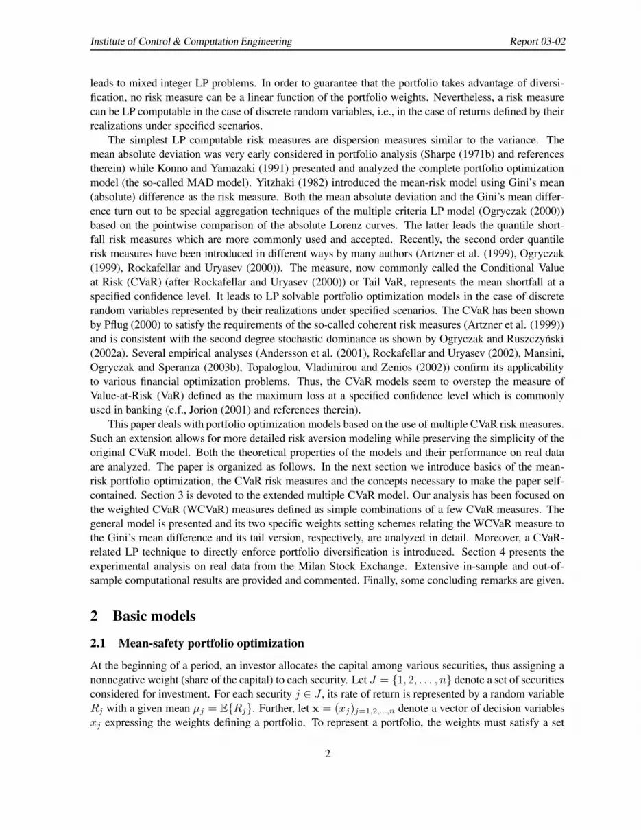
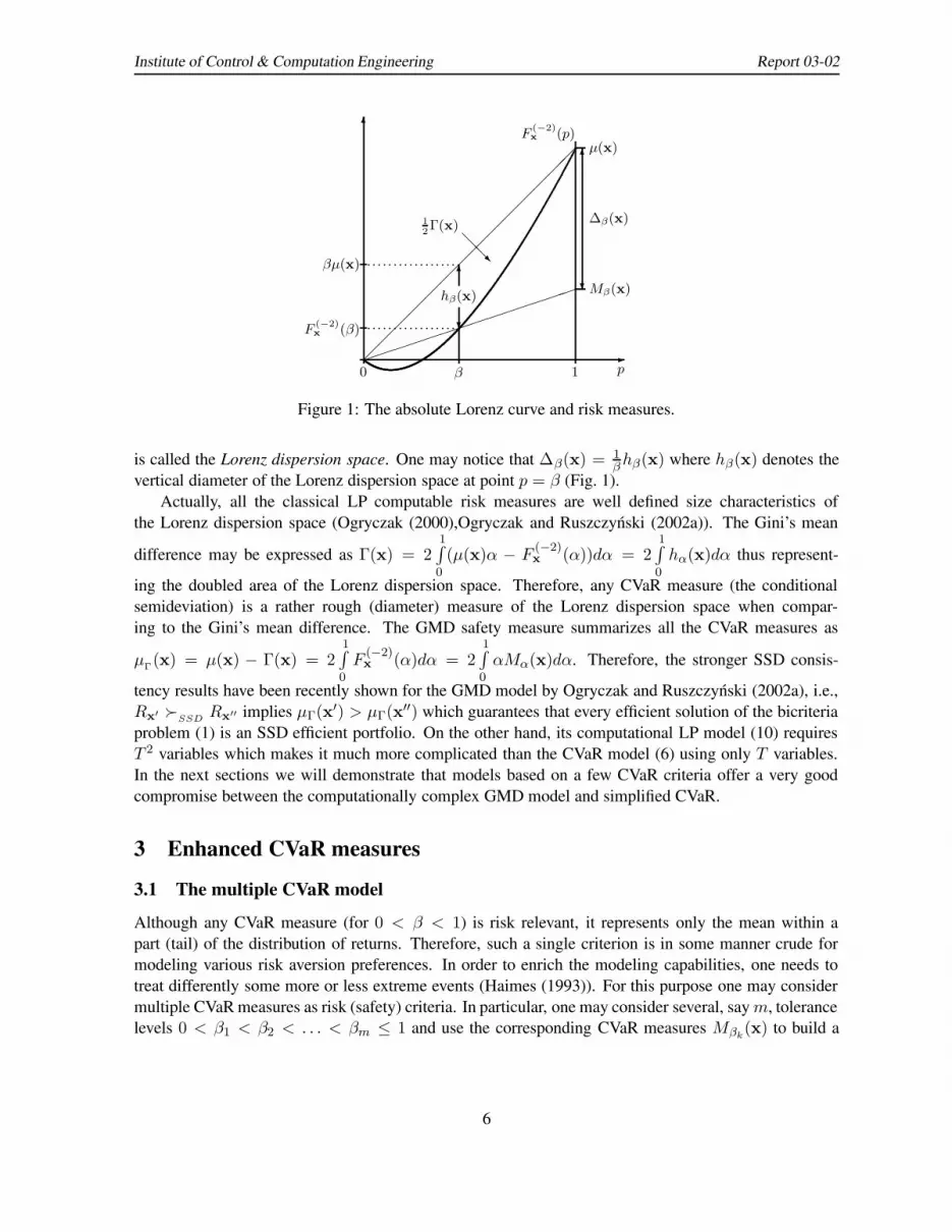
Figure 1: The absolute Lorenz curve and risk measures.

is called the Lorenz dispersion space. One may notice that ∆β(x) = 1βhβ(x) where hβ(x) denotes the

vertical diameter of the Lorenz dispersion space at point p = β (Fig. 1).Actually, all the classical LP computable risk measures are well defined size characteristics of

the Lorenz dispersion space (Ogryczak (2000),Ogryczak and Ruszczynski (2002a)). The Gini’s mean

difference may be expressed as Γ(x) = 21∫

0

(µ(x)α − F(−2)x (α))dα = 2

1∫

0

hα(x)dα thus represent-

ing the doubled area of the Lorenz dispersion space. Therefore, any CVaR measure (the conditionalsemideviation) is a rather rough (diameter) measure of the Lorenz dispersion space when compar-ing to the Gini’s mean difference. The GMD safety measure summarizes all the CVaR measures as

µΓ(x) = µ(x) − Γ(x) = 21∫

0

F(−2)x (α)dα = 2

1∫

0

αMα(x)dα. Therefore, the stronger SSD consis-

tency results have been recently shown for the GMD model by Ogryczak and Ruszczynski (2002a), i.e.,R

x′ �

SSDR

x′′ implies µΓ(x′) > µΓ(x′′) which guarantees that every efficient solution of the bicriteria

problem (1) is an SSD efficient portfolio. On the other hand, its computational LP model (10) requiresT 2 variables which makes it much more complicated than the CVaR model (6) using only T variables.In the next sections we will demonstrate that models based on a few CVaR criteria offer a very goodcompromise between the computationally complex GMD model and simplified CVaR.

3 Enhanced CVaR measures

3.1 The multiple CVaR model

Although any CVaR measure (for 0 < β < 1) is risk relevant, it represents only the mean within apart (tail) of the distribution of returns. Therefore, such a single criterion is in some manner crude formodeling various risk aversion preferences. In order to enrich the modeling capabilities, one needs totreat differently some more or less extreme events (Haimes (1993)). For this purpose one may considermultiple CVaR measures as risk (safety) criteria. In particular, one may consider several, say m, tolerancelevels 0 < β1 < β2 < . . . < βm ≤ 1 and use the corresponding CVaR measures Mβk

(x) to build a

6


multiple criteria portfolio selection model:

max{[Mβ1(x),Mβ2(x), . . . ,Mβm(x)] : x ∈ P}. (11)

The model may contain the original mean value as the last criterion M1(x) = µ(x), if βm = 1. Onemay notice that, for any portfolio x, one gets [Mβ1(x),Mβ2(x), . . . ,Mβm

(x)] ≤ [µ(x), µ(x), . . . , µ(x)]with at least one inequality strict. Hence, the multiple criteria model (11) is risk relevant in the sensethat for any risky portfolio its outcome vector is dominated by that for the risk-free portfolio with thesame expected return. Actually, the model (11) is SSD consistent in the sense that R

x′ �

SSDR

x′′ im-

plies [Mβ1(x′),Mβ2(x

′), . . . ,Mβm(x′)] ≥ [Mβ1(x

′′),Mβ2(x′′), . . . ,Mβm

(x′′)]. Actually, the followingassertion is valid.

Theorem 1 For any set of levels 0 < β1 < β2 < . . . < βm ≤ 1, except for portfolios with identicalvalues of all the corresponding CVaR measures Mβk

(x), every efficient solution of the multiple criteriaproblem (11) is an SSD efficient portfolio.

Proof. Let x0 ∈ P be an efficient solution of (11). Suppose that there exists x

′ ∈ P such thatR

x′ �

SSDR

x0 . Then, due to SSD consistency of the CVaR measures, Mβk

(x′) ≥ Mβk(x0) for all

k = 1, . . . ,m. The latter together with the fact that x0 is efficient, implies that Mβk(x′) = Mβk

(x0) fork = 1, . . . ,m, which completes the proof.

The weighted sum is the simplest aggregation technique in multiple criteria optimization. It can alsobe used to combine the CVaR criteria in (11). The weighted CVaR objective was first introduced byOgryczak (2000) (not using the name CVaR introduced later by Rockafellar and Uryasev (2000)); theportfolio optimization model based on historical data and its LP computability was then proven. Laterit was extended and considered in various forms for portfolio optimization (Ogryczak and Ruszczynski,2002b; Acerbi and Simonetti, 2002), general decisions under risk (Ogryczak, 2002), as well as for re-gression analysis (Rockafellar, Uryasev and Zabarankin, 2002).

In order to distinguish clearly the µ(x) criterion, further we will consider it separately from the mtolerance levels 0 < β1 < β2 < . . . < βm < 1 (thus excluding β = 1). Combining µ(x) and theCVaR values Mβk

(x) with positive (and normalized) weights we introduce the Weighted multiple CVaR(WCVaR) measure as

M(m)w (x) = w0µ(x) +

m∑

k=1

wkMβk(x)

m∑

k=0

wk = 1, w0 ≥ 0, wk > 0 for k = 1, . . . ,m.

(12)

The WCVaR measure is, obviously, a safety measure and it is risk relevant. The corresponding riskmeasure turns out to be the weighted sum of the ∆βk

(x) measures thus forming the weighted conditionalsemideviation:

∆(m)w (x) = µ(x) − M

(m)w (x) =

m∑

k=1

wk∆βk(x),

m∑

k=1

wk ≤ 1, wk > 0 for k = 1, . . . ,m. (13)

The latter is not affected by any shift of the outcome scale and it is equal to 0 in the case of a risk-freeportfolio while taking positive value for any risky portfolio, thus representing a translation invariant and

7


risk relevant dispersion parameter. Therefore, we can consider the corresponding Markowitz-type modeland its mean-safety formalization (1):

max{[µ(x),M(m)w (x)] : x ∈ P} = max{[µ(x), µ(x) − ∆

(m)w (x)] : x ∈ P}. (14)

Since the CVaR measures are coherent (Pflug, 2000) and SSD consistent (Ogryczak and Ruszczynski(2002a)), the same applies to the WCVaR measure. In particular, R

x′ �

SSDR

x′′ implies M

(m)w (x′) ≥

M(m)w (x′′) (Ogryczak and Ruszczynski (2002b)). Actually, the SSD consistency relation for the WCVaR

measure is stronger since it takes into account all the individual CVaR measures as shown in the followingassertion.

Theorem 2 For any set of levels 0 < β1 < β2 < . . . < βm ≤ 1, except for portfolios with identicalvalues of µ(x) and all conditional semideviations ∆βk

(x), respectively, every efficient solution of thebicriteria problem (14) is an SSD efficient portfolio.

Proof. Let x0 ∈ P be an efficient solution of (14). Suppose that there exists x′ ∈ P such that R

x′ �

SSD

Rx

0 . Then, due to SSD consistency of the CVaR measures, µ(x′) ≥ µ(x0) and Mβk(x′) ≥ Mβk

(x0) forall k = 1, . . . ,m. The latter, together with the fact that x

0 is efficient, implies that µ(x′) = µ(x0) and∑m

k=1 wkMβk(x′) =

∑mk=1 wkMβk

(x0). Hence, Mβk(x′) = Mβk

(x0) for k = 1, . . . ,m, and therefore,∆βk

(x′) = ∆βk(x0) for all k = 1, . . . ,m, which completes the proof.

For returns represented by their realizations we get an LP optimization problem. The model con-tains the following core LP constraints to define a feasible portfolio, portfolio realizations, and portfolioexpected return:

x ∈ P and z ≥ µ0,n

∑

j=1

µjxj = z andn

∑

j=1

rjtxj = yt for t = 1, . . . , T (15)

where z is an unbounded variable representing the mean return of the portfolio x and yt (t = 1, . . . , T )are unbounded variables to represent the realizations of the portfolio return under the scenario t.

The general WCVaR model (14) leads us to the following LP problem:

maximize w0z +m

∑

k=1

wkqk −m

∑

k=1

wk

βk

T∑

t=1

ptdtk

subject to (15) and dtk − qk + yt ≥ 0, dtk ≥ 0 for t = 1, . . . , T ; k = 1, . . . ,m

(16)

where qk (for k = 1, . . . ,m) are unbounded variables taking the values of the corresponding βk-quantiles(in the optimal solution). Except from the core constraints (15), model (16) contains T nonnegativevariables dtk and T corresponding linear inequalities for each k. Thus, its dimensionality is proportionalto the number of scenarios T and to the number of tolerance levels m. Note that model (16) with m = 1and w0 = 0 covers the standard CVaR model, while m > 1 and various settings of positive weightswk allow us to model a wide gamut of risk averse preferences. The model itself does not require anyspecific relation between the number of scenarios T and the number of securities n or the number oftolerance levels m. Certainly, similar to the Markowitz model, a very low number of scenarios mayresult in much less diversified portfolios. Increasing the number of tolerance levels m, generally, enablesa larger diversification. However, such diversification is not guaranteed since, as demonstrated later, italso depends on a specific weights setting.

8


Recall that the absolute Lorenz curve, and thereby the CVaR measures, represent a dual character-ization of the SSD relation (Ogryczak and Ruszczynski (2002a)). Hence, the weighted combination ofthe CVaR measures may be interpreted as the dual utility criterion within the theory developed by Yaari(1987) which was recently reintroduced into the finance literature in a simplified form of the spectral riskmeasures (Acerbi, 2002). Indeed, according to (12),

M(m)w (x) = w0

1∫

0

F(−1)x (α)dα +

m∑

k=1

wk

βk

βk∫

0

F(−1)x (α)dα =

1∫

0

φ(α)F(−1)x (α)dα

where

φ(α) =

w0 +

m∑

k=1

wk

βk, 0 < α ≤ β1

w0 +

m∑

k=i

wk

βk, βi−1 < α ≤ βi

w0, βm < α ≤ 1

(17)

is a decreasing risk aversion function (note the sign change for our safety measures to be maximized).As pointed out by Acerbi (2002), the subjective risk aversion of an investor can be encoded in a

function φ(α) defined for all possible confidence levels α ∈ (0, 1] and from a financial point of viewone cannot see any natural choice of function φ(α). The use of a wide class of risk aversion functions inportfolio optimization (Acerbi and Simonetti (2002)) seems to be rather far from the simplicity necessaryto make possible an effective implementation of the portfolio optimization procedure. In the followingwe will focus on the WCVaR measures defined as simple combinations of a very few CVaR measures(thus stepwise risk aversion functions φ with a very few steps). On the other hand, we introduce twospecific types of weights settings which relate the WCVaR measure to the Gini’s mean difference and itstail version. This allows us to use a few tolerance levels βk as the only parameters specifying the entireWCVaR measures (modeling risk aversion function) while the corresponding weights are automaticallypredefined by the requirements of the corresponding Gini’s measures. In other words, the investor’spreferences are modeled by a selection of a few tolerance levels. It turns out that we have managedto identify a class of simple WCVaR measures performing better in a real-life portfolio optimizationenvironment than typical CVaR measures and the GMD model itself.

3.2 Wide WCVaR measures

In the case of equally probable T scenarios with pt = 1/T (historical data for T periods), the weightedCVaR measure M

(T−1)w (x) defined with m = T − 1 tolerance levels βk = k/T for k = 1, 2, . . . , T − 1

represents the standard weighting approach in the multiple criteria LP portfolio optimization model withcriteria F (−2)(k/T ) (Ogryczak (2000)). The use of weights wk = (2k)/T 2 for k = 1, 2, . . . , T − 1

and w0 = 1/T results then in ∆(T−1)w (x) = 2

T

∑T−1k=1 h k

T

(x) = Γ(x) (c.f. Fig. 1). Hence, the WCVaRmodel is then equivalent to the GMD model. One may notice that LP formulation (16), similarly to theGMD one, requires T 2 linear inequalities. Hence, this very specific model cannot provide us with anynew modeling capabilities while causing a significant computational burden due to the large number ofCVaRs.

In the general case of T scenarios with arbitrary probabilities pt, one may use an approximationto Γ(x) with ∆

(m)w (x) based on some reasonably chosen grid of tolerance levels βk, k = 1, . . . ,m

9


and weights wk expressing the corresponding trapezoidal approximation to the integral formula Γ(x) =

2∫ 10 (µ(x)α−F

(−2)x (α))dα. Such an approximation is a very attractive risk measure itself as it allows us

to dramatically reduce the computational burden caused by T 2 dimensionality of the LP implementationof the GMD model (10) while introducing new modeling capabilities connected to the grid selection.Exactly, for any grid of m tolerance levels 0 < β1 < . . . < βk < . . . < βm < 1 one gets the trapezoidalapproximation:

Γ(x) ∼=

m∑

k=1

(βk+1 − βk−1)hβk(x) =

m∑

k=1

(βk+1 − βk−1)βk∆βk(x)

where β0 = 0 and βm+1 = 1. Note that∑m

k=1(βk+1 − βk−1)βk = βm < 1. This leads us to theweighted CVaR measure with weights defined as:

wk = (βk+1 − βk−1)βk, for k = 1, . . . ,m, and w0 = 1 − βm. (18)

Precisely, when using the weights given by (18), the corresponding WCVaR measure defined by (12)is an approximation to the GMD safety measure (9) (i.e., M

(m)w (x) ∼= µ

Γ(x)), and the corresponding

weighted conditional semideviation (13) is an approximation to the Gini’s mean difference itself (i.e.,∆

(m)w (x) ∼= Γ(x)). This can be also illustrated in terms of the spectral measures (Acerbi (2002)) as

integrating by parts one gets

µΓ(x) = 2

1∫

0

F(−2)x (α)dα = 2αF

(−2)x (α)

]1

0− 2

1∫

0

αF(−1)x (α)dα

= 2F(−2)x (1) − 2

1∫

0

αF(−1)x (α)dα =

1∫

0

2(1 − α)F(−1)x (α)dα

which allows us to express the GMD safety measure by the risk aversion function φ(α) = 2(1−α) whileformula (17) with the weights (18) defines a stepwise approximation to this function.

Again, the WCVaR measures may be considered the exact GMD measure applied to (m + 1)-pointdistributions approximating the original distribution of returns Rx, thus providing a trapezoidal ap-proximation to the original Lorenz dispersion space. In particular, for the (m + 1)-point distributionR

x(β1,...,βm)

P{Rx

(β1,...,βm) = ξ} =

β1, ξ = a1

βk − βk−1, ξ = ak for k = 1, . . . ,m1 − βm, ξ = am+1

0, otherwise

such that a1 ≤ a2 ≤ . . . ≤ am+1, the weighted conditional semideviation ∆(m)w (x(β1,...,βm)) with

weights (18) is equal to the Gini’s mean difference Γ(x(β1,...,βm)). In general, ∆(m)w (x) is a lower ap-

proximation to Γ(x) (∆(m)w (x) ≤ Γ(x)) and thereby M

(m)w (x) ≥ µΓ(x).

It must be emphasized that despite being only an approximation to the Gini’s mean difference, anyWCVaR measure with weights defined by (18) is a well defined LP computable risk measure with guar-anteed SSD consistency in the sense of Theorem 2. In other words, we are interested in the GMD ap-proximation properties only for a reasonable weights definition. We will refer to the WCVaR measures

10


with weights defined by (18) as the Wide WCVaR as covering (spanning) a wide area of the quantilescale. The wide WCVaR measures need not to employ a very dense grid to provide a proper modelingof risk averse preferences. This allows us to build relatively small LP models with mT variables. In ourcomputational analysis we have considered m = 3 while testing three different patterns of the tolerancelevels (see Table 1) corresponding to three types of preferences defined by the tolerance levels location.

3.3 Tail WCVaR measures

The Wide WCVaR measures, based on the approximation to the Gini’s measure, contain the risk neutralterm M1(x) = µ(x) with the weight w0 = 1−βm. This may cause the measure to pay too much attentionto very low probable but very large returns. Actually, the measure can be more sensitive to large returnsthan the Gini’s mean difference itself. We encountered such a situation in our computational analysiswhere in a few cases all the models based on the WCVaR approximation to GMD selected a singlesecurity portfolio with very high expectation caused by a very few but extremely high return realizations.

In order to overcome this flaw one may use the Tail WCVaR measures, built with an approximation tothe tail GMD measures instead of the GMD itself. The tail Gini’s measure (Ogryczak and Ruszczynski(2002a, 2002b)) defined for any β ∈ (0, 1] by averaging the vertical diameters hp(x) within the tailinterval p ≤ β as:

Γβ(x) =2

β2

β∫

0

(µ(x)α − F(−2)x (α))dα. (19)

A simple analysis of the absolute Lorenz curve (Ogryczak and Ruszczynski (2002a)) shows that, forany 0 < β ≤ 1, the tail Gini’s measure Γβ(x) is SSD safety consistent. One may notice that thecorresponding safety measure µ

Γβ(x) = µ(x) − Γβ(x) can be expressed as

µΓβ

(x) = µ(x) −2

β2

β∫

0

(µ(x)α − F(−2)x (α))dα =

2

β2

β∫

0

F(−2)x (α)dα

which allows us to consider it as a second degree CVaR measure.In the simplest case of equally probable T scenarios with pt = 1/T , the tail Gini’s measure for

β = K/T may be expressed as the weighted conditional semideviation ∆(K)w (x) with tolerance levels

βk = k/T for k = 1, 2, . . . ,K and properly defined weights (Ogryczak and Ruszczynski (2002a)). Ina general case, we may resort to an approximation with the weighted CVaR measure based on somereasonably chosen grid βk, k = 1, . . . ,m and weights wk expressing the corresponding trapezoidalapproximation of the integral in the formula (19). Exactly, for any 0 < β ≤ 1, while using the grid of mtolerance levels 0 < β1 < . . . < βk < . . . < βm = β one may define the weights:

wk =(βk+1 − βk−1)βk

β2, for k = 1, . . . ,m − 1, and wm =

(βm − βm−1)βm

β2(20)

where β0 = 0. This results in the weighted sum∑m

k=1 wk∆βk(x) expressing the trapezoidal approx-

imation to the tail Gini’s measure (19). Note that∑m

k=1 wk = β2m/β2 = 1 and thus we get a regular

weighted conditional semideviation (13) ∆(m)w (x) ∼= Γβ(x). Further, weights (20) together with w0 = 0

generate a WCVaR measure (12) such that M(m)w (x) ∼= µ

Γβ(x). This can be also illustrated in terms of

11


the spectral measures (Acerbi (2002)) as integrating by parts one gets

µΓβ(x) =

2

β2

β∫

0

F(−2)x (α)dα =

2

β2αF

(−2)x (α)

]β

0

−2

β2

β∫

0

αF(−1)x (α)dα

=2

βF

(−2)x (β) −

2

β2

β∫

0

αF(−1)x (α)dα =

1∫

0

2(β − α)+

β2F

(−1)x (α)dα

allowing us to express the tail GMD safety measure by the risk aversion function φ(α) = 2(β −α)+/β2

where (.)+ denotes the nonnegative part of a number. Formula (17) with the weights (20) define astepwise approximation to this function.

Again, we emphasize that despite being only an approximation to (19), any Tail WCVaR measure(e.g., a WCVaR measure with weights defined according to (20)) is a well defined LP computable mea-sure with guaranteed SSD consistency in the sense of Theorem 2. They need not be built on a very densegrid to provide proper modeling of risk averse preferences. Actually, we are interested in a direct pref-erence modeling with simple Tail WCVaR measures rather than strict approximation to the Tail GMDmeasure. In our computational analysis we have tested two Tail WCVaR models with m = 2 and m = 3.Obviously, all the Tail WCVaR models measure are implemented as LP problems (16) but with w0 = 0.Again, for a small value of m we get rather small LP models with mT variables.

3.4 Direct diversification enforcement

Since the seminal work of Markowitz (1952), the notion of investing in diversified portfolios is consid-ered one of the most fundamental concepts of portfolio management. Diversification should be enforcedby the mean/risk preference model. Indeed, in the original Markowitz model it was usually guaranteedby the standard deviation (variance) minimization. In general, it may happen that a single security or alow diversified portfolio is SSD dominating over all other (more diversified) portfolios, and the SSD con-sistent Markowitz-type models will select such an undiversified solution. Especially, the SSD consistentmodels based on the LP computable risk measures may fail to generate sufficiently diversified portfolios,although it also happens for the original Markowitz model (Mansini, Ogryczak and Speranza (2003b)).Therefore, additional restrictions may be posed on the feasible portfolios to guarantee the required di-versification. The simplest way to enforce portfolio diversification is to limit the maximum share. This,however, allows us to form a portfolio with a few shares at the maximum level. A better modeling alter-native would be to allow for a relatively large maximum share provided that the other shares are smaller.Such a rich diversification scheme may be introduced with the CVaR constructs applied to the right tailof the distribution of shares.

A natural generalization of the maximum share is the (right-tail) conditional mean defined as themean within the specified tolerance level (amount) of the worst shares. One may simply define theconditional mean as the mean of the k largest shares. This can be formalized as follows. First, weintroduce the ordering map Θ : Rn → Rn such that Θ(x) = (θ1(x), θ2(x), . . . , θn(x)), where θ1(x) ≥θ2(x) ≥ · · · ≥ θn(x) and there exists a permutation τ of set J such that θj(x) = xτ(j) for j = 1, . . . , n.The use of ordered outcome vectors Θ(x) allows us to focus on distributions of shares impartially. Next,the linear cumulative map is applied to ordered vectors to get Θ(x) = (θ1(x), θ2(x), . . . , θn(x)) defined

12


as

θk(x) =

k∑

j=1

θj(x), for k = 1, . . . , n.

The coefficients of vector Θ(x) express, respectively: the largest share, the total of the two largest shares,the total of the three largest shares, etc. Hence, the (worst) k

n–conditional mean share is given as 1k θk(x),

for k = 1, . . . , n.Similar to the CVaR formulas, for a given vector x, the value of θk(x) may be found by solving the

linear program (Ogryczak and Tamir (2003)):

θk(x) = min {ksk +

n∑

j=1

dskj : ds

kj ≥ xj − sk, dskj ≥ 0 for j = 1, . . . , n},

where sk is an unbounded variable (representing the k-th largest share at the optimum) and dskj are

additional nonnegative (deviational) variables. Hence, any model under consideration can easily beextended with direct diversification constraints specified as θk(x) ≤ ck and implemented with linearinequalities:

ksk +

n∑

j=1

dskj ≤ ck and ds

kj ≥ xj − sk, dskj ≥ 0 for j = 1, . . . , n. (21)

4 Experimental analysis

4.1 Testing environment

The present section is devoted to the experimental analysis in a real framework of all the describedLP models based on extensions of the CVaR measure. Models have been tested on a PC with a 500MHz Pentium processor by using CPLEX 6.5 package. First we present the test problems, then theresults of the in-sample analysis, both on the original models and on their modifications to enforcediversification, are described. Finally, the out-of-sample results are analyzed and the results obtainedthrough the simulation of a ”multiperiod-type” portfolio investment are presented.

Historical data are represented by weekly rates of return obtained by using stock prices from MilanStock Exchange. The rates are computed as relative price variations. Dividends are not included. Thedata set consists of 157 securities quoted with continuity from 1994 to 1999. In the first years of thishistorical period the Italian Stock Exchange has shown alternate short periods of up and down trendswhile entering a positive growing trend at the end. This is shown in Figure 2, where the performance ofthe Milan Stock Exchange index MIB30 is depicted in the period (1994–1999).

A set of 13 instances has been created, each of which takes into account the complete set of securitiesover a different time period. For this reason, from now on, we will indifferently refer to them as instancesor periods. In particular, each instance is based on two years realizations (about 104 weekly observations)as in-sample period and one year as out-of-sample. The choice of weekly periodicity is consistent withthe objective of reducing estimation errors through an adequate number of observations (Simaan (1997)).Two consecutive instances differ from each other for a three months period, e.g. the first instance coversthe two years 1994–1995 as in-sample period, while the second instance does not include the first threemonths of 1994 and does include the first three months of 1996. For each instance the Maximum Safety

13


Figure 2: The Milan Stock Exchange Index (MIB30) in the years 1994–1999 (weekly quotations).

Portfolio (MSP) has been obtained through the use of the various tested models. In this section we onlysummarize and comment the main figures out of the huge amount of computational results we obtained.

The model introduced by Young (1998), with safety measure the maximization of the worst realiza-tion (7), is identified as Minimax. The model based on the safety measure corresponding to the Gini’smean difference (10), i.e. the mean worse return, is referred simply as GMD. The CVaR model asso-ciated to a given tolerance level β is identified as CVaR(β). We have tested the CVaR model for fivedifferent values of β, i.e. CVaR(0.05), CVaR(0.1), CVaR(0.25), CVaR(0.5) and CVaR(0.75). All theCVaR and the weighted CVaR models have been formulated according to (16). The weighted CVaRmodels representing an approximation to the Gini’s measure (the Wide CVaR models) have been testedwith m = 3 tolerance weights. Such models have been identified as WCVaR(AGD), WCVaR(AGS) andWCVaR(AGT). The corresponding models weights are summarized in Table 1. Finally, we have also

Table 1: Wide Weighted CVaR models

Model Tolerance levels Weightsw0 w1 w2 w3

WCVaR(AGD): Downside Approximationβ1 = 0.1, β2 = 0.25, β3 = 0.5 0.5 0.025 0.1 0.375

WCVaR(AGS): Symmetric Approximationβ1 = 0.25, β2 = 0.5, β3 = 0.75 0.25 0.125 0.25 0.375

WCVaR(AGT): Tails Approximationβ1 = 0.1, β2 = 0.5, β3 = 0.9 0.1 0.05 0.4 0.45

tested two Tail WCVaR models:

• Model WCVaR(TG2) with two tolerance levels β1 = 0.1, β2 = 0.25 and weights w1 = 0.4 and

14


w2 = 0.6.

• Model WCVaR(TG3) with three tolerance levels β1 = 0.1, β2 = 0.25, β3 = 0.5 and weightsw1 = 0.1, w2 = 0.4 and w3 = 0.5.

Since SSD consistent models based on the LP computable risk measures may fail to generate diver-sified enough portfolios we have added the following additional restrictions to guarantee the requireddiversification: any stock share cannot exceed 0.20, while any three shares cannot exceed 0.50 in totaland any six shares cannot globally exceed 0.75 of the portfolio investment. This requires the followingside constraints on the shares to be added:

xj ≤ 0.2 for j = 1, . . . , n

3s3 +

n∑

j=1

ds3j ≤ 0.5 and ds

3j ≥ xj − s3, ds3j ≥ 0 for j = 1, . . . , n

6s6 +

n∑

j=1

ds6j ≤ 0.75 and ds

6j ≥ xj − s6, ds6j ≥ 0 for j = 1, . . . , n

(22)

For each model we have tested the corresponding version obtained by adding constraints (22).

4.2 In-sample analysis

In the following we present and comment the characteristics of the MSPs selected by the different modelswith and without the introduction of diversification enforcement. In Table 2, the complete computationalresults for model CVaR(0.1) are presented as an example of the type of information obtained by solvinga single model over all the 13 periods. The table consists of a first part corresponding to the results forthe models without diversification enforcement and a second one for the models with the diversificationenforcement constraints (22). Each of the two parts of the table has five columns: the objective functionvalue (obj.), the portfolio per cent mean return (z), the portfolio diversification (div.) represented by thenumber of selected securities, the minimum and the maximum share within the portfolio, respectively.The average return is given on a weekly basis (a good yearly approximation can be obtained by mul-tiplying the figures by 52). Notice that the introduction of diversification constraints may result in anunmodified optimal portfolio. This is the case for the portfolios selected in the instances 7 and 8. Similarresults are shown in Table 3 for the model WCVaR(AGD).

To simplify results presentation, we have decided to focus our attention only on a subset of instances(periods). In Tables 4-6 we show the results obtained by the different models in the first, the sixth and thetwelfth instance without and with diversification constraints. The tables have the same structure of Tables2-3. Tables 4 and 5 show the large values obtained by the Wide WCVaR: the fact can be explained bythe relevance given to high returns by these models which are much more sensitive to large returns thanthe Gini’s mean difference itself. This also explains why, in some instances (see, for instance, Table 3),the Wide WCVaR models select only a one security portfolio characterized by a large expected return(about 94% per week) generated by very few realizations with dramatically high return. Moreover, itis worth noticing that in the Wide WCVaR models the mean return z value is larger than that of all theother models. This is also true in the twelfth period where the returns are dramatically lower than in otherperiods, thus reflecting the downwards trend of the whole market. From Tables 4-6 and the analogousresults obtained for the other periods we observed that the MSPs mean return tends to increase over theyears by reaching a pick in the first quarter of the year 1998 and then decreasing. This allows us todraw some conclusions on market trend. In general, the basic CVaR models are the most diversified.

15


Table 2: CVaR(0.1) model without and with diversification constraints: optimal portfolio characteristicsin each of the 13 periods.

without diversification with diversificationperiods obj. z div. shares obj. z div. shares

10−2 % # min max 10−2 % # min max

1 -1.567 0.21 18 1.77 10−3 0.293 -1.638 0.17 20 1.93 10−3 0.2002 -1.543 0.24 18 2.09 10−3 0.281 -1.604 0.21 20 4.45 10−4 0.2003 -1.129 0.61 18 3.33 10−3 0.204 -1.137 0.52 20 1.10 10−3 0.1924 -0.999 0.19 23 1.68 10−3 0.144 -0.999 0.19 23 1.68 10−3 0.1445 -0.955 0.10 24 6.24 10−3 0.138 -0.955 0.10 24 8.28 10−3 0.1386 -0.736 0.43 26 1.18 10−4 0.165 -0.736 0.43 26 1.18 10−4 0.1327 -0.721 0.41 27 1.48 10−4 0.112 -0.721 0.41 27 1.48 10−4 0.1128 -0.649 0.54 27 1.53 10−3 0.138 -0.649 0.54 27 1.53 10−3 0.1389 -0.560 0.61 29 7.64 10−4 0.128 -0.560 0.61 29 7.64 10−4 0.128

10 -0.549 1.01 24 2.07 10−3 0.121 -0.549 1.01 24 2.07 10−3 0.12111 -1.401 0.99 19 7.81 10−5 0.245 -1.412 0.98 20 1.05 10−3 0.20012 -2.188 0.91 18 1.11 10−4 0.210 -2.188 0.91 18 1.11 10−4 0.21013 -2.476 0.90 17 4.49 10−3 0.223 -2.478 0.87 18 5.30 10−4 0.200

Moreover, in some of these models (see CVaR(0.05) and CVaR(0.1)) the introduction of constraints (22)results in no further diversification (see Table 5).

In the following the main figures obtained for all the selected portfolios are summarized. Table 7shows, for all the models over all the periods, the diversification of the optimal portfolios (MSPs). Forinstance, the number of selected securities for the Minimax model varies, out of the 13 solved instances,from 6 to 29 securities, while with the introduction of diversification constraints the corresponding rangebecomes 12–29. Similar considerations can be made by analyzing portfolios composition in terms ofminimum and maximum portfolio shares. On average, the Wide WCVaR provide the ranges with thelowest upper limits and result in extremely low diversified portfolios (or rather undiversified portfoliosas the lower limit can be equal to 1). These models seem to require the use of an additional technique toguarantee enough diversification. Also the Minimax model may generate some low diversified portfolios(6 securities). The other models have always selected more than 10 securities. Nevertheless, in manycases they generated portfolios with very large shares (exceeding 30%) of particular securities. Thus,for all the LP computable models under consideration we may recommend a support of some directtechnique for diversification enforcement. One may notice that the application of the CVaR based diver-sification enforcement constraints (22) has resulted in portfolios always containing at least 10 securities.

4.3 Out-of-sample analysis

In this section the behavior of all the MSPs is examined in the twelve months following the date ofeach portfolio selection. To describe out-of-sample results we have used the following nine ex-post pa-rameters: the minimum, the average, the maximum and the median portfolio return (rmin, rav, rmax

and rmed, respectively); the standard deviation (std) and the semi-standard deviation (s-std); the meanabsolute deviation (MAD) and the mean downside semideviation (s-MAD); the maximum downside de-viation (D-DEV). Such performance criteria have been computed for all the models over all the periodsand can be used to compare the out-of-sample behavior of the maximum safety portfolios selected by thedifferent models. The minimum, average, maximum and median ex-post portfolio returns are expressed

16


Table 3: WCVaR(AGD) without and with diversification constraints: optimal portfolio characteristics ineach of the 13 periods.

without diversification with diversificationperiods obj. z div. shares obj. z div. shares

10−2 % # min max 10−2 % # min max

1 40.577 94.26 1 1 1 8.422 19.52 12 1.49 10−2 0.2002 40.464 93.88 1 1 1 8.462 19.57 11 1.56 10−2 0.2003 42.558 95.04 1 1 1 8.842 19.67 12 4.34 10−3 0.2004 42.467 95.21 1 1 1 8.804 19.64 14 3.63 10−3 0.2005 42.991 95.46 1 1 1 8.881 19.55 19 8.29 10−4 0.2006 45.953 97.16 1 1 1 9.535 20.06 15 8.77 10−3 0.2007 0.270 1.11 15 1.18 10−3 0.204 0.270 1.10 16 8.12 10−4 0.2008 0.313 1.19 17 7.29 10−3 0.198 0.313 1.19 17 7.29 10−3 0.1989 0.332 1.00 21 4.53 10−3 0.106 0.332 1.00 21 4.53 10−3 0.106

10 0.673 1.57 21 2.49 10−3 0.148 0.673 1.57 21 2.49 10−3 0.14811 0.405 1.51 16 6.30 10−3 0.168 0.405 1.51 16 6.30 10−3 0.16812 0.182 1.51 17 2.71 10−3 0.179 0.182 1.51 17 2.71 10−3 0.17913 0.219 1.87 14 1.32 10−2 0.237 0.217 1.84 15 8.64 10−3 0.200

Table 4: Period 1 - Maximum Safety Portfolios: optimal portfolio characteristics.without diversification with diversification

models obj. z div. shares obj. z div. shares10−2 % # min max 10−2 % # min max

Minimax -1.812 0.06 14 1.40 10−3 0.193 -1.823 0.12 16 3.98 10−4 0.194CVaR(0.05) -1.767 0.15 14 5.14 10−3 0.214 -1.789 0.13 16 3.06 10−3 0.187CVaR(0.1) -1.567 0.21 18 1.77 10−3 0.293 -1.638 0.17 20 1.93 10−3 0.200CVaR(0.25) -1.155 0.29 11 1.57 10−3 0.316 -1.199 0.29 18 5.13 10−3 0.200CVaR(0.5) -0.597 0.39 17 3.31 10−5 0.288 -0.611 0.40 19 4.87 10−5 0.200CVaR(0.75) -0.055 0.62 17 1.12 10−4 0.179 -0.056 0.61 18 1.18 10−4 0.172GMD -0.313 0.60 17 2.60 10−4 0.246 -0.318 0.61 18 7.90 10−4 0.200WCVaR(AGD) 40.577 94.26 1 1 1 8.422 19.52 12 1.49 10−2 0.200WCVaR(AGS) 16.147 94.26 1 1 1 3.532 19.48 13 1.19 10−2 0.200WCVaR(AGT) 1.603 94.26 1 1 1 0.632 19.47 13 2.74 10−3 0.200WCVaR(TG2) -1.393 0.21 16 1.34 10−3 0.343 -1.455 0.16 18 2.63 10−3 0.200WCVaR(TG3) -0.986 0.31 15 8.99 10−5 0.304 -1.025 0.36 18 2.60 10−5 0.200

on a yearly basis. All the dispersion measures (std, s-std, MAD, s-MAD and D-DEV) have been com-puted with respect to the target return µ0 (which is zero for the MSP) to make them directly comparablein the different models.

In Tables 8 and 9 we present the average value of each criterion, over the thirteen periods, for thevarious models in the cases without and with diversification enforcement, respectively. One may no-tice extremely high average returns of the Wide WCVaR models (without diversification enforcement).These performances are produced by single security portfolios with very high returns. In general, themodels are too risky as demonstrated by all the dispersion measures. When we consider the models withdiversification enforcement (Table 9), the Wide WCVaR models are still characterized by the highestaverage returns and the largest dispersion parameters but the differences from the other models are notvery large. One may notice that the GMD model, which is the computationally most complex, may beeasily outperformed (in terms of average returns and dispersion) by the simpler Tail WCVaR models oreven by the CVaR(0.5) model.

17




Minimax -0.745 0.45 27 2.31 10−4 0.169 -0.745 0.45 27 2.31 10−4 0.169CVaR(0.05) -0.745 0.45 27 2.31 10−4 0.169 -0.745 0.45 27 2.31 10−4 0.169CVaR(0.1) -0.736 0.43 26 1.18 10−4 0.164 -0.736 0.43 26 1.18 10−4 0.164CVaR(0.25) -0.613 0.44 22 1.27 10−5 0.112 -0.613 0.44 22 1.27 10−5 0.112CVaR(0.5) -0.246 2.64 26 3.30 10−3 0.180 -0.246 2.64 26 3.30 10−3 0.180CVaR(0.75) 0.262 7.33 21 3.72 10−4 0.229 0.260 7.01 21 6.88 10−3 0.200GMD 0.060 9.12 20 4.30 10−3 0.178 0.060 9.12 20 4.11 10−3 0.178WCVaR(AGD) 45.953 97.16 1 1 1 9.535 20.06 15 8.77 10−3 0.200WCVaR(AGS) 21.599 97.16 1 1 1 4.651 20.01 16 6.17 10−3 0.200WCVaR(AGT) 7.504 97.16 1 1 1 1.868 20.07 14 2.41 10−5 0.200WCVaR(TG2) -0.693 0.44 27 1.19 10−4 0.151 -0.693 0.44 27 1.19 10−4 0.151WCVaR(TG3) -0.514 1.61 26 1.47 10−3 0.107 -0.514 1.61 26 1.47 10−3 0.107



Minimax -2.848 0.99 13 3.77 10−3 0.289 -2.927 0.99 14 1.41 10−3 0.200CVaR(0.05) -2.486 0.88 14 1.09 10−3 0.198 -2.488 0.88 15 1.51 10−3 0.200CVaR(0.1) -2.188 0.91 18 1.11 10−4 0.210 -2.188 0.90 18 9.13 10−4 0.200CVaR(0.25) -1.529 0.94 20 4.65 10−3 0.134 -1.529 0.94 20 4.65 10−3 0.134CVaR(0.5) -0.608 1.05 20 7.87 10−4 0.129 -0.608 1.05 20 7.87 10−4 0.129CVaR(0.75) 0.204 1.35 14 4.30 10−4 0.222 0.203 1.35 14 3.99 10−3 0.200GMD -0.186 1.35 20 1.01 10−2 0.129 -0.186 1.35 20 1.01 10−2 0.129WCVaR(AGD) 0.182 1.51 17 2.71 10−3 0.179 0.182 1.51 17 2.71 10−3 0.179WCVaR(AGS) -0.028 1.39 18 6.10 10−3 0.158 -0.028 1.39 18 6.10 10−3 0.158WCVaR(AGT) 0.029 1.41 20 3.36 10−3 0.135 0.029 1.41 20 3.36 10−3 0.135WCVaR(TG2) -1.882 0.99 18 1.25 10−3 0.187 -1.882 0.99 18 1.25 10−3 0.187WCVaR(TG3) -1.270 0.99 23 1.47 10−4 0.131 -1.270 0.99 23 1.47 10−4 0.131

We have also analyzed each model performance with respect to a long-run portfolio management.Each of the portfolios selected by a specific model in the 13 instances has been evaluated ex-post inthe three months period following the date of selection. Tables 10 and 11 provide the single periodreturns (each column corresponds to a different period from 1 to 13) for each model without and withthe diversification enforcement, respectively. It is worth noticing that single period ex-post returns quiteperfectly represent the upward and downward movements of the market. For instance, the negative resultsshowed by all the models in the periods 3 and 4 are mainly due to the negative trend of the market in1996, especially in the period from April to July and then again in October. However, we noticed that insuch periods some models (such as CVaR(0.1) and CVaR(0.25)) find portfolios with a better performancewith respect to the market index MIB30. Similarly, for the periods 10-11 and partially 12 which sufferedthe negative fall of the market in the second quarter of the 1998 and then again in August. Finally, thehigh returns in period 9 can be partially interpreted as a consequence of the positive trend of the marketat the beginning of the 1998 with a high positive jump of the MIB30 index performances in March (see

18


Table 7: Diversification of the optimal portfolios (MSPs).MSP without MSP with

models diversification enforcement diversification enforcement

Minimax 6–29 12–29CVaR(0.05) 14–29 15–29CVaR(0.1) 17–29 18–29CVaR(0.25) 11–30 18–30CVaR(0.5) 16–29 18–27CVaR(0.75) 12–23 13–22GMD 12–26 16–26WCVaR(AGD) 1–21 11–21WCVaR(AGS) 1–23 13–21WCVaR(AGT) 1–25 11–25WCVaR(TG2) 15–30 17–30WCVaR(TG3) 15–29 16–29

Table 8: Out-of-sample statistics for MSPs: average values over the 13 periods.Without diversification enforcement

models rmin rav rmed rmax std s-std MAD s-MAD D-DEV

Minimax -54.36 30.05 17.57 337.19 0.0614 0.0270 0.0493 0.0148 0.0749CVaR(0.05) -52.75 28.77 10.66 332.93 0.0596 0.0264 0.0477 0.0145 0.0720CVaR(0.1) -52.43 30.57 12.24 347.98 0.0611 0.0263 0.0486 0.0141 0.0713CVaR(0.25) -49.68 34.27 26.58 307.67 0.0591 0.0237 0.0454 0.0110 0.0718CVaR(0.5) -53.10 31.12 32.34 282.05 0.0603 0.0267 0.0474 0.0128 0.0788CVaR(0.75) -59.86 27.80 29.34 381.36 0.0668 0.0325 0.0512 0.0161 0.0945GMD -58.64 27.85 26.21 315.79 0.0639 0.0304 0.0495 0.0151 0.0870WCVaR(AGD) -72.84 92.27 48.52 3625.59 0.1153 0.0427 0.0913 0.0218 0.1148WCVaR(AGS) -71.69 94.00 47.57 3634.52 0.1152 0.0415 0.0907 0.0209 0.1136WCVaR(AGT) -72.17 94.15 49.47 3631.79 0.1151 0.0418 0.0908 0.0209 0.1146WCVaR(TG2) -52.14 30.52 27.86 378.51 0.0614 0.0259 0.0473 0.0134 0.0719WCVaR(TG3) -49.50 33.09 25.23 321.26 0.0602 0.0243 0.0458 0.0116 0.0719

Figure 2). In such period many models find higher returns with respect to the MIB30 index.Further, we cumulated the returns over the horizon up to 13 periods (39 months) to better analyze

each model achievements. The figures shown in Table 12 are the cumulative returns of the portfoliosselected by each model in the case without diversification enforcement. Table 13 provides the sameresults for the case with diversification enforcement. Each column of these tables refers to a periodand provides the cumulative returns of the portfolios selected over the preceding periods. For a betterunderstanding of these figures let us consider the first line of Table 12 which refers to the model Minimax.Each of the 13 portfolios selected by the Minimax model in the 13 instances has been evaluated ex-postin the three months investment period following the date of its selection. Let us define as r1, r2, ..., r13

the ex-post returns of these 13 portfolios (their values are shown in the first line of Table 10). Then,the first column of Table 12 gives the ex-post return (after 3 months) of the first portfolio selected, i.e.r1 (notice that such value is identical in Tables 12 and 10). The second column of Table 12 gives thecumulative return of the portfolio selected in the first period and then modified after three months withthe portfolio selected in the second period: the value is computed as (1 + r1)(1 + r2) − 1. Similarly, forall the other columns of the table. These results have been computed to simulate a multi-period settingwhere, at no transaction cost, the portfolio changes over time. Rates are expressed on a yearly basis.

19


Table 9: Out-of-sample statistics for MSPs: average values over the 13 periods.With diversification enforcement

models rmin rav rmed rmax std s-std MAD s-MAD D-DEV

Minimax -53.80 31.38 25.49 337.79 0.0607 0.0263 0.0486 0.0139 0.0735CVaR(0.05) -53.27 28.73 13.78 329.62 0.0592 0.0264 0.0473 0.0143 0.0731CVaR(0.1) -52.17 29.88 11.94 334.94 0.0596 0.0259 0.0474 0.0138 0.0712CVaR(0.25) -46.93 33.00 26.57 302.67 0.0581 0.0232 0.0444 0.0109 0.0678CVaR(0.5) -53.50 30.49 32.33 289.09 0.0607 0.0268 0.0470 0.0129 0.0793CVaR(0.75) -60.23 28.56 29.34 384.64 0.0682 0.0333 0.0522 0.0163 0.0948GMD -59.19 27.50 27.78 323.99 0.0646 0.0308 0.0497 0.0153 0.0877WCVaR(AGD) -63.43 35.21 38.88 439.76 0.0742 0.0337 0.0582 0.0171 0.0947WCVaR(AGS) -62.91 36.75 36.00 426.09 0.0737 0.0327 0.0574 0.0162 0.0944WCVaR(AGT) -62.67 36.96 38.21 426.26 0.0735 0.0328 0.0575 0.0162 0.0945WCVaR(TG2) -52.04 30.19 27.86 366.65 0.0608 0.0257 0.0466 0.0132 0.0719WCVaR(TG3) -49.36 31.62 25.44 322.26 0.0600 0.0246 0.0452 0.0119 0.0718

Table 10: Out-of-sample results for MSPs: single period returns.Without diversification enforcement

models 1 2 3 4 5 6 7 8 9 10 11 12 13

Minimax 54.09 13.15 -16.33 -2.41 62.07 33.31 39.77 85.43 348.50 -24.86 -60.31 0.99 10.33CVaR(0.05) 63.87 11.71 -16.33 -2.41 62.07 33.31 39.77 85.43 348.50 -24.86 -49.44 -2.84 9.51CVaR(0.1) 64.54 11.80 -10.97 -4.88 65.87 27.61 39.23 78.16 352.58 -25.94 -48.17 -7.46 39.95CVaR(0.25) 73.05 4.27 -5.02 -0.40 80.39 38.78 20.16 71.22 392.11 10.28 -54.66 31.95 34.90CVaR(0.5) 96.96 20.96 -21.01 -4.74 52.95 41.05 10.14 58.21 434.77 7.51 -55.21 39.74 58.90CVaR(0.75) 148.85 32.11 -13.21 -19.60 58.17 48.33 11.85 37.56 519.56 2.30 -58.02 87.45 4.59GMD 128.21 29.54 -14.26 -18.64 60.09 77.01 9.75 36.80 431.47 10.76 -53.08 47.40 10.33WCVaR(AGD) 322.73 1221.48 -13.19 79.75 245.78 186.20 12.80 39.12 442.15 3..11 -52.42 44.00 10.33WCVaR(AGS) 322.73 1221.48 -13.19 79.75 245.78 186.20 7.30 40.06 440.93 0.26 -55.78 57.47 10.46WCVaR(AGT) 322.73 1221.48 -13.19 79.75 245.78 186.20 12.76 29.69 453.65 8..57 -54.52 40.90 17.69WCVaR(TG2) 53.17 1.84 -11.14 -1.79 81.30 30.09 28.27 71.23 385.45 -17.94 -47.15 10.67 140.90WCVaR(TG3) 78.91 12.06 -11.77 -6.49 77.17 42.13 21.41 52.27 404.90 7.78 -53.40 29.80 66.31

Table 12 shows extremely high cumulated returns of the Wide WCVaR models (without diversifi-cation enforcement). These performances are due to the single security portfolios selected in the first 6periods which resulted in dramatically high returns. Actually, when ignoring these 6 periods and focus-ing on the remaining horizon of the last 21 months, the cumulative returns of the Wide WCVaR modelsconsiderably shrink as it is evident when comparing the first part of Table 14 with the last seven columnsof Table 12. Table 14 shows the ex-post cumulated returns over the last 21 months (7 periods) both forthe case without and with diversification enforcement. Moreover, as in column (7–13) of the first part ofTable 14, it can be noticed that the Wide WCVaR models perform much worse than all the other modelsexcept for the Minimax and the extremal CVaR models (β = 0.05 or β = 0.1). Note that both the TailWCVaR models and the CVaR(0.5) here have the best cumulative performances.

When the models with diversification enforcement are considered (see Table 13), the Wide WCVaRmodels are still characterized by the highest cumulative returns but the differences from the other modelsare not very large. When ignoring the first 6 periods and focusing on the last 21 months (second partof Table 14), one may see again the Wide WCVaR models performing much worse than all the othermodels except for the Minimax and the extremal CVaR models. It is interesting to notice that, except for

20


Table 11: Out-of-sample results for MSPs: single period returns.With diversification enforcement

models 1 2 3 4 5 6 7 8 9 10 11 12 13

Minimax 67.81 13.26 -26.42 -2.25 62.07 33.31 39.77 85.43 348.50 -24.86 -61.65 -11.03 -0.52CVaR(0.05) 57.11 16.46 -26.42 -2.25 62.07 33.31 39.77 85.43 348.50 -24.86 -54.08 -2.95 6.28CVaR(0.1) 48.16 11.85 -15.53 -4.88 65.87 27.61 39.23 78.16 352.58 -25.94 -49.31 -7.63 25.82CVaR(0.25) 71.10 4.17 -12.74 -0.40 80.39 38.78 20.16 71.22 392.11 10.28 -54.02 31.95 34.90CVaR(0.5) 100.55 15.53 -21.94 -5.39 52.93 41.05 10.14 58.21 434.77 7.51 -55.21 39.74 58.90CVaR(0.75) 145.52 29.29 -13.17 -21.09 57.85 46.87 16.47 37.56 519.56 2.30 -59.99 89.12 8.76GMD 127.84 20.23 -18.40 -20.27 59.58 76.91 10.92 36.80 431.47 10.76 -52.45 47.40 10.39WCVaR(AGD) 184.78 107.76 -23.10 -6.83 84.90 85.39 12.68 39.12 442.15 3.11 -52.42 44.00 9.76WCVaR(AGS) 170.49 100.48 -21.68 -6.28 86.56 93.73 10.06 40.06 440.93 0.26 -55.32 57.47 11.57WCVaR(AGT) 173.36 101.80 -21.99 -7.87 95.32 98.48 13.00 29.69 453.65 8.57 -54.52 40.90 17.69WCVaR(TG2) 50.35 7.30 -14.16 -1.79 81.30 30.09 28.27 71.23 385.45 -17.94 -47.30 10.67 129.28WCVaR(TG3) 81.68 7.66 -15.61 -6.41 77.17 42.13 21.41 52.27 404.90 7.78 -56.11 29.80 66.31

Table 12: Out-of-sample results for MSPs: cumulative returns.Without diversification enforcement

models 3 m. 6 m. 9 m. 12 m. 15 m. 18 m. 21 m. 24 m. 27 m. 30 m. 33 m. 36 m. 39 m.

Minimax 54.09 32.04 13.41 9.23 18.20 20.59 23.16 29.63 48.80 38.97 24.00 21.90 20.97CVaR(0.05) 63.87 35.30 15.27 10.57 19.36 21.58 24.03 30.42 49.60 39.65 27.33 24.49 23.27CVaR(0.1) 64.54 35.63 17.87 11.72 20.91 22.00 24.33 30.04 49.37 39.25 27.28 23.95 25.11CVaR(0.25) 73.05 34.33 19.67 14.30 25.23 27.39 26.33 31.22 51.98 47.19 32.25 32.22 32.43CVaR(0.5) 96.96 54.35 23.46 15.71 22.35 25.29 23.00 26.93 48.93 44.15 29.62 30.43 32.43CVaR(0.75) 148.85 81.32 41.84 23.07 29.40 32.38 29.23 30.24 54.89 48.60 32.46 36.35 33.60GMD 128.21 71.94 36.35 19.84 26.98 34.21 30.41 31.19 53.25 48.36 33.61 34.71 32.66WCVaR(AGD) 322.73 647.41 264.67 205.56 213.21 208.53 167.22 146.28 168.85 144.28 110.52 103.96 94.55WCVaR(AGS) 322.73 647.41 264.67 205.56 213.21 208.53 165.32 144.96 167.49 142.49 107.74 102.99 93.71WCVaR(AGT) 322.73 647.41 264.67 205.56 213.21 208.53 167.21 144.12 167.38 144.33 109.71 102.87 94.55WCVaR(TG2) 53.17 24.90 11.50 8.02 19.80 21.46 22.41 27.66 48.08 39.59 27.80 26.27 32.71WCVaR(TG3) 78.91 41.59 20.94 13.41 23.99 26.85 26.05 29.07 50.19 45.29 31.02 30.92 33.35

the Minimax and the extremal CVaR models, all the other models resulted in similar cumulative returnover the entire horizon of 39 months with (annual) rate of return exceeding 30%. Also the GMD modelis outperformed by simple Tail WCVaR models and the CVaR models for larger tolerance levels.

To better capture the models behavior over small periods with possibly different market trends wehave analyzed the ex-post cumulative returns over subperiods of length 4, that is we computed the cumu-lative returns over the periods 7–10, 8–11, 9–12 and 10–13. In Table 15 we have shown the minimum, theaverage and the maximum cumulative return (rcmin, rcav, and rcmax, respectively) for each model overthese subperiods. Note that during the periods with negative market trend, as during subperiod 10–13, allthe models have negative average cumulative returns. However, GMD and CVaR(0.5) and CVaR(0.25)show the best, although negative, average performance. Moreover, when the maximum cumulative re-turn is considered, the three best models are GMD, CVaR(0.25) and WCVaR(TG3), respectively. On thecontrary, in positive market trend periods such as in the subperiod 9-12 (corresponding to the first part ofthe year 1998), the CVaR(0.75) has the largest average and maximum cumulative return while the largestminimum cumulative return is obtained by GMD.

Finally, to show how consistently the composition of the portfolios selected by the same model

21


Table 13: Out-of-sample results for MSPs: cumulative returns.With diversification enforcement


Minimax 67.81 37.87 11.83 8.13 17.25 19.78 22.45 28.97 48.13 38.41 23.16 19.87 18.16CVaR(0.05) 57.11 35.26 10.42 7.11 16.36 19.03 21.79 28.36 47.50 37.88 24.77 22.18 20.88CVaR(0.1) 48.16 28.73 11.86 7.42 17.17 18.85 21.57 27.52 46.79 37.08 25.23 22.09 22.38CVaR(0.25) 71.10 33.50 15.86 11.56 22.82 25.34 24.59 29.64 50.35 45.76 31.25 31.31 31.58CVaR(0.5) 100.55 52.22 21.84 14.37 21.21 24.32 22.18 26.19 48.16 43.48 29.07 29.93 31.95CVaR(0.75) 145.52 78.16 40.21 21.44 27.98 30.95 28.78 29.84 54.46 48.23 31.59 35.63 33.35GMD 127.84 65.51 30.75 15.54 23.25 30.90 27.84 28.93 50.90 46.31 32.10 33.31 31.39WCVaR(AGD) 184.78 143.24 65.70 43.49 50.95 56.21 49.09 47.81 70.77 62.37 45.22 45.12 42.03WCVaR(AGS) 170.49 132.87 61.94 41.25 49.33 55.95 48.38 47.31 70.22 61.44 43.65 44.75 41.88WCVaR(AGT) 173.36 134.87 62.66 41.11 50.59 57.68 50.35 47.60 70.96 63.37 45.44 45.06 42.74WCVaR(TG2) 50.35 27.01 11.46 7.99 19.78 21.44 22.39 27.64 48.06 39.58 27.75 26.23 32.16WCVaR(TG3) 81.68 39.85 18.18 11.49 22.31 25.41 24.83 27.97 49.05 44.30 29.50 29.52 32.04

Table 14: Out-of-sample computational results: cumulative returns over the latest 21 months (7 periods).Without diversification With diversification

periods 7 7-8 7-9 7-10 7-11 7-12 7-13 7 7-8 7-9 7-10 7-11 7-12 7-13models

Minimax 39.77 60.99 115.24 71.91 28.23 23.22 22.83 39.77 60.99 115.24 71.91 27.35 19.96 16.79CVaR(0.05) 39.77 60.99 115.24 71.91 34.59 27.47 24.74 39.77 60.99 115.24 71.91 32.02 25.42 22.49CVaR(0.1) 39.23 57.50 112.92 69.81 33.93 25.93 27.84 39.23 57.50 112.92 69.81 33.34 25.42 25.48CVaR(0.25) 20.16 43.44 106.15 8.28 38.32 37.24 36.90 20.16 43.44 106.15 8.28 38.70 37.55 37.17CVaR(0.5) 10.14 32.00 100.87 77.91 35.02 35.79 38.88 10.14 32.00 100.87 77.91 35.02 35.79 38.88CVaR(0.75) 11.85 24.04 102.30 76.72 32.56 40.44 34.65 16.47 26.58 104.88 78.51 32.37 40.48 35.43GMD 9.75 22.53 91.36 72.42 32.90 35.21 31.34 10.92 23.18 92.00 72.88 33.55 35.76 31.81WCVaR(AGD) 12.80 25.27 95.24 72.10 33.08 34.84 29.74 12.68 25.20 95.17 72.05 33.05 34.81 30.91WCVaR(AGS) 7.30 22.59 92.48 68.97 29.23 33.56 29.98 10.06 24.15 94.01 70.04 30.16 34.36 30.84WCVaR(AGT) 12.76 20.93 92.24 72.19 31.94 33.39 31.03 13.00 21.06 92.37 72.28 32.00 33.44 31.07WCVaR(TG2) 28.27 48.21 109.51 71.99 35.84 31.28 43.17 28.27 48.21 109.51 71.99 35.76 31.21 42.10WCVaR(TG3) 21.41 35.97 100.98 78.10 36.20 35.12 39.19 21.41 35.97 100.98 78.10 34.59 33.78 38.00

over the different periods may change, we have reported, as an example, Table 16 which provides theportfolios composition changes from one period to the other for the portfolios selected by the differentmodels in the case without diversification enforcement. For instance, the second line of Table 16 refersto model CVaR(0.05) and can be interpreted as follows. The first column gives the number of securitiesselected by this model in the first period (in this case 14 securities). The second column says that, withrespect to the previous portfolio, the one selected in the second period contains 2 new securities and nosecurities have been eliminated from those already selected. Similarly for the other models.

4.4 Models behavior in a strong downward trend period: the years 2000-2002

The Markowitz type models, used without any additional forecasting procedure applied prior to portfolioselection process itself, do not recognize any market trends and therefore they are generally not appro-priate tools for investment situations with a long lasting market trend. Nevertheless, due to commonlyobserved negative trends during recent years, both researchers and practitioners become more interested

22


Table 15: Cumulative return statistics in subperiods of length 4: case without diversification.7-10 8-11 9-12 10-13

models rcmin rcav rcmax rcmin rcav rcmax rcmin rcav rcmax rcmin rcav rcmax

Minimax 39.77 71.98 115.24 24.42 93.88 188.38 3.55 110.99 348.50 -46.32 -33.69 -24.86CVaR(0.05) 39.77 71.98 115.24 30.15 95.31 188.38 10.70 114.35 348.50 -41.26 -29.46 -22.76CVaR(0.1) 39.23 69.87 112.92 31.90 92.20 183.96 11.93 116.40 352.58 -38.73 -27.90 -18.73CVaR(0.25) 8.28 44.51 106.15 43.77 101.49 190.28 33.07 148.21 392.11 -28.79 -8.21 10.28CVaR(0.5) 10.14 55.23 100.87 42.07 97.63 190.87 34.39 161.67 434.77 -30.61 -8.27 7.51CVaR(0.75) 16.47 56.61 104.88 36.67 90.73 191.93 33.75 188.27 519.56 -36.02 -11.41 2.30GMD 10.92 49.75 92.00 36.80 84.56 169.64 37.94 163.64 431.47 -27.42 -7.01 10.76WCVaR(AGD) 12.68 51.28 95.17 38.69 85.57 174.63 35.75 163.56 442.15 -29.96 -10.83 3.11WCVaR(AGS) 10.06 49.57 94.01 35.73 84.87 175.25 31.87 161.36 440.93 -33.07 -12.24 0.26WCVaR(AGT) 13.00 49.68 92.37 29.69 81.21 167.96 36.93 168.97 453.65 -29.73 -9.19 8.57WCVaR(TG2) 28.27 64.50 109.51 37.70 94.87 188.31 23.46 133.65 385.45 -34.24 -17.60 2.35WCVaR(TG3) 21.41 59.12 100.98 38.10 90.32 177.28 31.27 150.53 404.90 -31.22 -9.27 7.78

Table 16: Out-of-sample computational results: changes in portfolios composition.Without diversification enforcement


Minimax 14 3, -1 14,-11 9,-7 10, -5 7, -6 11, -11 9, -7 13, -13 3, -6 3, -23 8, -1 3, -8CVaR(0.05) 14 2, 0 12,-9 9,-7 10, -5 7, -6 11, -11 9, -7 13, -13 3, -6 10, -19 8, -11 7, -5CVaR(0.1) 18 9, -9 12,-7 5,-4 8, -6 13, -12 8, -8 15, -13 2, -7 0, -24 11, -16 12, -13 8, -9CVaR(0.25) 11 2, -1 10,-4 10,-6 8, -8 6, -6 10, -6 8, -8 12, -9 6, -5 2, -15 9, -6 6, -6CVaR(0.5) 17 2, -3 14,-14 17,-14 9, -4 7, -5 8, -12 8, -9 10, -4 10, -10 5, -12 6, -6 4, -5CVaR(0.75) 17 3, -5 4,-5 4,-3 7, -2 7, -6 1, -10 8, -2 6, -2 8, -10 6, -11 7, -8 3, -4GMD 17 1, -6 7,-5 4,-3 10, -3 5, -7 4, -8 10, -4 6, -2 8, -11 5, -9 6, -5 3, -7WCVaR(AGD) 1 0,0 0,0 0,0 0,0 0,0 14, 0 6, -4 7, -3 6, -6 4, -9 5, -4 3, -6WCVaR(AGS) 1 0,0 0,0 0,0 0,0 0,0 15, 0 9, -4 8, -6 8, -9 5, -10 6, -5 2, -6WCVaR(AGT) 1 0,0 0,0 0,0 0,0 0,0 16, 0 8, -5 9, -4 5, -9 5, -10 6, -2 2, -6WCVaR(TG2) 16 7,-9 9,-9 7,-6 10,-3 7,-6 12, -9 7, -9 12, -13 1, -1 7, -13 12, -15 7, -10WCVaR(TG3) 15 5,-2 5,-5 9,-6 9,-5 6,-5 8, -5 7, -8 7, -8 6, -5 2, -9 9, -7 4, -6

in the models behavior under such circumstances. Therefore, in order to provide a better analysis andcomparison of the proposed models when the market trend is negative and thus the risk control may berelevant, we have decided to add some computational results on the period (2000-2002). During thisperiod the Italian market has shown an impressive and continuous down-turn (see Figure 3) with theMIB30 index reaching its highest level 50467 on 10.03.2000 and its lowest level 21546 on 4.10.2002.

The following tables provide the relevant results on the analysis of the Maximum Safety Portfolios(MSPs) selected by the different models with and without diversification enforcement using the years2000-2001 (104 weekly returns) as in-sample period and the year 2002 as out-of-sample. As for previousresults, historical data are stock prices from Milan Stock Exchange. The new data set consists of 178securities quoted with continuity from 2000 to 2002. The meaning of tables entries is identical to thosedescribed in the former sections. Due to low weekly values, the mean return z has been converted on ayearly basis.

Notice that all the models but CVaR(0.75), GMD and the Wide WCVaR models have a mean returnequal to zero. Thus, as for previous experiments, the Wide WCVaR models are still among those modelswith larger mean returns. The use of constraints that force diversification improves, on average, the

23


Figure 3: The Milan Stock Exchange Index (MIB30) in the years 2000–2002 (weekly quotations).

portfolios performance in terms of mean return: CVaR(0.75) shows an increase from 1.83% to 3.27%,while some models as CVaR(0.5) and CVaR(0.25) move from null to positive values. The same effectwas not evident in the previous experiments.

Table 17 shows that with respect to portfolio diversification, the introduction of enforcementconstraints produces an evident effect only for the Minimax model and the extremal CVaR models(CVaR(0.05) and CVaR(0.1)). As before (see Tables 4-6), the Minimax model generates some lowdiversified portfolios (7 securities). In contrast to previous results the basic CVaR models are not themost diversified: the CVaR(0.05) model has selected only 6 securities, while the CVaR(0.1) portfolio has8 securities. Moreover, note that the Wide WCVaR models have selected rather diversified portfolios ifwe compare these results with those shown in Tables 4-6. During the period 2000-2002 no security hasshown realizations with dramatically high returns, thus justifying this diversification. Finally, in onlyone case, i.e. for the WCVaR(TG3) model, the diversification without enforcement is larger than thatobtained with additional forcing constraints. In the first part of Table 17 it is worth noticing that all theselected portfolios have a maximum share exceeding 40% (but for the model WCVaR(AGD) with 38%)and that, in two cases, namely for the models Minimax and CVaR(0.05), the maximum share is largerthan 80% and 55%, respectively. For all such models we may recommend to apply the enforcementconstraints (22) giving as result portfolios always containing at least 11 securities.

For the out-of-sample analysis the behavior of all the MSPs is examined in the 52 weeks followingthe date of each portfolio selection. The nine parameters reported in Tables 18 and 19 have the samemeaning defined for previous similar tables. Again, rmin, rav , rmed and rmax are expressed on a yearlybasis and as per cent returns. Due to general market downward trend, all the portfolios show ex-postnegative average returns: the model CVaR(0.75) has the worst performance.

By comparing Table 18 with Table 19 one may notice that, on average, the introduction of diver-

24


Table 17: In-sample MSPs characteristics: strong downward trend period.without diversification with diversification


Minimax -0.212 0.00 7 2.06 10−4 0.813 -0.281 0.00 14 6.01 10−4 0.2CVaR(0.05) -0.189 0.00 6 2.17 10−3 0.563 -0.231 0.00 11 8.83 10−4 0.2CVaR(0.1) -0.158 0.00 8 2.38 10−4 0.450 -0.193 0.00 16 7.62 10−5 0.2CVaR(0.25) -0.107 0.00 13 1.61 10−4 0.469 -0.129 0.11 15 2.47 10−4 0.2CVaR(0.5) -0.065 0.00 13 1.69 10−4 0.459 -0.079 0.16 13 5.48 10−5 0.2CVaR(0.75) -0.031 1.83 15 1.70 10−3 0.463 -0.033 3.27 19 1.83 10−3 0.2GMD -0.050 0.10 13 2.97 10−4 0.464 -0.058 0.60 15 1.48 10−3 0.2WCVaR(AGD) -0.039 0.50 15 2.15 10−4 0.384 -0.044 1.16 17 7.25 10−5 0.2WCVaR(AGS) -0.044 0.25 15 1.46 10−4 0.432 -0.050 0.81 16 1.24 10−3 0.2WCVaR(AGT) -0.043 0.34 15 1.10 10−5 0.495 -0.049 1.08 15 1.42 10−3 0.2WCVaR(TG2) -0.131 0.00 12 7.28 10−5 0.429 -0.158 0.00 15 1.15 10−4 0.2WCVaR(TG3) -0.093 0.00 14 1.59 10−4 0.444 -0.112 0.06 12 3.50 10−3 0.2

Table 18: Out-of-sample results for MSPs: strong downward trend period.Max. safety Without diversification enforcementmodel rmin rav rmed rmax std s-std MAD s-MAD D-DEVMinimax -14.18 -0.93 -0.68 14.01 0.0009 0.0007 0.0006 0.0004 0.0029CVaR(0.05) -12.81 -0.73 -0.79 13.66 0.0009 0.0006 0.0007 0.0004 0.0026CVaR(0.1) -7.81 -0.58 -1.19 10.70 0.0008 0.0006 0.0006 0.0004 0.0016CVaR(0.25) -10.16 -0.88 -1.11 12.93 0.0008 0.0006 0.0006 0.0004 0.0021CVaR(0.5) -8.75 -0.68 -0.96 13.25 0.0008 0.0006 0.0006 0.0004 0.0018CVaR(0.75) -48.42 -1.49 0.67 42.82 0.0031 0.0026 0.0021 0.0012 0.0126GMD -9.97 -0.76 -0.61 13.21 0.0009 0.0007 0.0007 0.0004 0.0020WCVaR(AGD) -15.44 -1.01 -0.76 14.91 0.0011 0.0009 0.0008 0.0005 0.0032WCVaR(AGS) -12.77 -0.80 -0.33 12.44 0.0010 0.0008 0.0008 0.0005 0.0026WCVaR(AGT) -17.13 -0.94 -0.42 14.57 0.0012 0.0010 0.0009 0.0005 0.0036WCVaR(TG2) -7.61 -0.63 -0.59 11.56 0.0008 0.0006 0.0006 0.0004 0.0015WCVaR(TG3) -8.98 -0.77 -1.18 12.42 0.0008 0.0006 0.0006 0.0004 0.0018

sification enforcement may result in portfolios with larger ex-post dispersion. This is especially truefor those models whose dispersion was already high without enforcement (see, for instance, the modelsCVaR(0.75) and CVaR(0.5) in Table 18). When we consider the models with diversification enforcement(Table 19), the model WCVaR(TG3) has the highest average return. As for previous computational re-sults, the GMD model (which is the computationally most complex) is outperformed in terms of averagereturns and dispersion by the Tail WCVaR models.

Tables 20 and 21 show the ex-post cumulative portfolio returns for the case without and with thediversification enforcement, respectively. Additionally, the cumulative performances of the index MIB30has been introduced in both tables. The weighted CVaR models show a very stable ex-post performancealways outperforming GMD model. Moreover, the Wide WCVaR models also outperform extremalCVaR models when diversification enforcement is introduced (see Table 21). Actually, except for a shortperiod of strong increase of the MIB30 index, all the models outperform the index. When comparingTable 20 to Table 21 it is evident how diversification enforcement has, on average, positively contributedto improve all the portfolios performance with the only exception of extremal CVaR portfolios whoseperformances are worsen with respect to the case without diversification.

25


Table 19: Out-of-sample results for MSPs: strong downward trend period.Max. safety With diversification enforcementmodel rmin rav rmed rmax std s-std MAD s-MAD D-DEVMinimax -22.28 -0.96 -0.50 20.97 0.0013 0.0010 0.0009 0.0005 0.0048CVaR(0.05) -12.44 -1.23 -1.27 9.63 0.0008 0.0007 0.0006 0.0004 0.0025CVaR(0.1) -9.78 -0.97 -1.29 9.13 0.0008 0.0006 0.0006 0.0004 0.0020CVaR(0.25) -9.40 -0.61 -0.46 7.70 0.0008 0.0006 0.0006 0.0004 0.0019CVaR(0.5) -12.04 -0.75 -0.59 7.89 0.0008 0.0007 0.0006 0.0004 0.0025CVaR(0.75) -62.78 -1.96 -0.07 68.23 0.0044 0.0036 0.0030 0.0017 0.0188GMD -13.35 -0.89 -0.32 13.77 0.0011 0.0009 0.0008 0.0005 0.0027WCVaR(AGD) -24.45 -1.31 -0.57 22.34 0.0016 0.0013 0.0012 0.0007 0.0054WCVaR(AGS) -15.93 -0.95 -0.31 16.85 0.0013 0.0010 0.0009 0.0006 0.0033WCVaR(AGT) -23.55 -1.22 -0.19 21.53 0.0016 0.0013 0.0011 0.0007 0.0051WCVaR(TG2) -10.16 -0.77 -0.55 7.96 0.0008 0.0006 0.0006 0.0004 0.0021WCVaR(TG3) -9.82 -0.57 -0.61 8.30 0.0007 0.0006 0.0006 0.0003 0.0020

Table 20: Cumulative out-of-sample results: strong downward trend period.Without diversification enforcement

models 4 w. 8 w. 12 w. 16 w. 20 w. 24 w. 28 w. 32 w. 36 m. 40 w. 44 w. 48 w. 52 w.

Minimax 3.35 -3.41 4.23 1.55 0.74 -3.25 -7.25 -7.97 -7.81 -10.04 -5.94 -2.94 -0.93CVaR(0.05) 2.51 -2.99 5.89 2.72 2.21 -0.70 -4.58 -6.96 -6.81 -9.18 -5.22 -2.12 -0.73CVaR(0.1) 0.43 -4.33 5.44 2.86 2.63 -0.18 -4.44 -6.40 -6.42 -8.71 -5.17 -1.88 -0.58CVaR(0.25) -2.68 -8.19 -3.22 -3.62 -4.73 -5.08 -8.33 -9.31 -9.43 -13.40 -8.57 -3.29 -0.88CVaR(0.5) -2.13 -4.90 0.22 0.22 -1.60 -2.78 -5.85 -7.69 -7.74 -12.29 -7.66 -2.79 -0.68CVaR(0.75) 17.33 15.44 45.49 41.16 59.95 38.90 24.21 10.89 4.31 -15.59 -5.71 -1.24 -1.51GMD -0.66 -5.09 2.02 0.76 0.76 -0.26 -4.38 -6.71 -7.36 -11.91 -7.14 -2.48 -0.76WCVaR(AGD) 1.27 -4.44 4.99 4.13 6.31 2.31 -2.74 -5.48 -6.84 -14.40 -8.10 -3.13 -1.01WCVaR(AGS) 1.08 -3.04 5.50 4.14 4.98 2.20 -2.73 -5.46 -6.43 -12.11 -6.90 -2.40 -0.80WCVaR(AGT) 0.47 -3.79 4.66 3.65 5.22 3.65 -2.24 -5.68 -7.03 -13.90 -7.90 -2.69 -0.94WCVaR(TG2) -0.36 -5.68 1.84 -0.16 -0.22 -1.59 -4.64 -6.43 -6.91 -9.72 -5.92 -2.09 -0.63WCVaR(TG3) -2.21 -7.20 -1.09 -2.04 -2.94 -3.48 -6.82 -8.46 -8.57 -12.29 -7.67 -2.84 -0.78

MIB30 -26.71 -95.69 174.00 181.75 -45.95 -98.92 -99.43 -99.17 -98.68 -99.47 -94.31 -64.90 -26.45

The additional experimental analysis over the period 2000-2002 has allowed us to draw the followingmain conclusions. First, during strongly negative market trend the weighted CVaR models have, onaverage, performed better than the GMD, the Minimax and the extremal CVaR models. Actually, interms of cumulative returns all the models have beaten the MIB30 index performance. Second, duringstrongly negative market trend the Wide WCVaR models show a more stable behavior than in positivetrend period. In the latter case they may need diversification enforcement. Generally, the diversificationenforcement turns out to be necessary and effective for all the models rather during unstable market trends(typically characterized by quick changes of market directions, as for previous experiments) than duringstrong downward periods where for some models, as for the extremal CVaR models, diversificationenforcement has made performances poorer.

26


Table 21: Cumulative out-of-sample results: strong downward trend period.With diversification enforcement

models 4 w. 8 w. 12 w. 16 w. 20 w. 24 w. 28 w. 32 w. 36 m. 40 w. 44 w. 48 w. 52 w.

Minimax -0.75 -4.82 12.72 11.80 10.55 1.85 -4.21 -7.25 -6.69 -11.67 -5.87 -2.31 -0.96CVaR(0.05) -4.84 -9.82 -1.42 -0.97 -4.50 -8.01 -11.31 -12.39 -11.18 -16.41 -11.07 -5.25 -1.23CVaR(0.1) -5.40 -10.72 0.10 0.42 -2.35 -8.70 -10.86 -11.93 -10.62 -15.59 -9.66 -4.33 -0.97CVaR(0.25) -1.62 -6.07 2.01 4.28 1.91 -3.73 -6.71 -7.62 -7.01 -12.35 -6.88 -2.79 -0.61CVaR(0.5) -2.31 -5.92 0.14 2.34 -0.97 -3.33 -6.26 -7.56 -7.33 -13.61 -8.25 -3.54 -0.75CVaR(0.75) 29.69 22.69 82.34 78.72 117.34 63.31 43.86 23.26 11.48 -16.54 -4.62 -0.52 -2.01GMD 0.80 -2.78 6.71 7.48 7.35 2.54 -1.51 -4.45 -5.77 -13.97 -7.52 -3.08 -0.89WCVaR(AGD) 4.66 0.53 12.61 12.57 15.39 7.67 2.73 -2.26 -4.96 -16.82 -8.60 -3.70 -1.31WCVaR(AGS) 2.80 -0.74 11.03 11.14 11.93 5.67 0.88 -2.62 -4.92 -14.34 -7.47 -2.93 -0.95WCVaR(AGT) 4.61 0.71 13.05 13.34 17.08 9.66 3.25 -2.18 -4.68 -16.98 -8.45 -3.41 -1.23WCVaR(TG2) -3.09 -7.69 1.66 3.54 -0.08 -5.82 -8.53 -9.56 -8.50 -14.06 -8.42 -3.61 -0.78WCVaR(TG3) -1.93 -5.78 1.83 3.83 0.72 -1.63 -4.97 -6.59 -6.44 -11.68 -6.82 -2.69 -0.57

MIB30 -26.71 -95.69 174.00 181.75 -45.95 -98.92 -99.43 -99.17 -98.68 -99.47 -94.31 -64.90 -26.45

5 Concluding remarks

In this paper we have studied LP solvable portfolio optimization models based on extensions of theConditional Value at Risk (CVaR) measure. The models use multiple CVaR measures thus allowing formore detailed risk aversion modeling. All the studied models are SSD consistent and may be consideredsome approximations to the Gini’s mean difference with the advantage of being computationally muchsimpler than the GMD model itself. Our analysis has been focused on the weighted CVaR measuresdefined as simple combinations of a very few CVaR measures. We have introduced two specific typesof weights settings which relate the WCVaR measure to the Gini’s mean difference (the Wide WCVaR)and its tail version (the Tail WCVaR). This allows us to use a few tolerance levels as only parametersspecifying the entire WCVaR measures while the corresponding weights are automatically predefined bythe requirements of the corresponding Gini’s measures.

Our experimental analysis of the models performance on the real-life data from the Milan StockExchange has confirmed their attractiveness. The weighted CVaR models have usually performed betterthan the GMD itself, the Minimax or the extremal CVaR models. These promising results show a needfor further comprehensive experimental studies analyzing practical performances of the weighted CVaRmodels within specific areas of financial applications. It is important to notice that although the quantilerisk measures (VaR and CVaR) were introduced in banking as extreme risk measures for very smalltolerance levels (like β = 0.05), for the portfolio optimization good results have been provided byrather larger tolerance levels. Additional experimental analysis over the period 2000-2002 with stronglynegative market trend has confirmed good achievements of the weighted CVaR models They have, onaverage, performed better than the GMD, the Minimax and the extremal CVaR models. In terms ofcumulative returns all the models have outperformed the MIB30 index.

While the Tail WCVaR models have always generated well diversified portfolios, the Wide WCVaRmodels require some diversification enforcement to avoid too small portfolios. Our experiments have alsoconfirmed effectiveness of our CVaR based technique for a direct diversification enforcement. Although,the diversification enforcement turns out to be necessary and effective rather during unstable markettrends (typically characterized by quick changes of market directions, as for previous experiments) than

27


during strong downward periods.

Appendix

The spectral risk measures have been shown to be coherent in the sense of Artzner et al. (1999). Thesecoherence axioms are based on the standard ‘monotonicity’ (X ≥ Y a.s. ⇒ ρ(X) ≤ ρ(Y )). Since themeasures represent the dual theory of choice (Yaari (1987)), they should also satisfy stronger monotonic-ity related to the SSD dominance. Indeed, the following SSD consistency results can be shown.

Theorem 3 If a nonnegative real function φ on the interval [0, 1] is weakly decreasing (i.e., 0 ≤ α1 <

α2 ≤ 1 implies φ(α1) ≥ φ(α2)), then the spectral measure Mφ(x) =1∫

0

φ(α)F(−1)x (α)dα is SSD

consistent, i.e.,R

x′ �

SSDR

x′′ ⇒ Mφ(x′) ≥ Mφ(x′′).

Proof. Note that

Mφ(x′) − Mφ(x′′) =

1∫

0

φ(α)(F(−1)x′ (α) − F

(−1)x′′ (α))dα

and integrating by parts one gets

Mφ(x′) − Mφ(x′′) = φ(1)(F(−2)x′ (1) − F

(−2)x′′ (1)) −

1∫

0

(F(−2)x′ (α) − F

(−2)x′′ (α))dφ(α) (23)

If Rx′ �

SSDR

x′′ , then F

(−2)x′ (α) ≥ F

(−2)x′′ (α) for all α ∈ [0, 1] and, in particular, F

(−2)x′ (1)−F

(−2)x′′ (1) =

µ(x′) − µ(x′′) ≥ 0. Hence, due to assumed properties of function φ, one gets Mφ(x′) − Mφ(x′′) ≥ 0,which completes the proof.

Theorem 4 If a nonnegative real function φ on the interval [0, 1] is strictly decreasing (i.e., 0 ≤ α1 <

α2 ≤ 1 implies φ(α1) > φ(α2)), then the spectral measure Mφ(x) =1∫

0

φ(α)F(−1)x (α)dα is strictly SSD

consistent, i.e.,R

x′ �

SSDR

x′′ ⇒ Mφ(x′) > Mφ(x′′).

Proof. If Rx′ �

SSDR

x′′ , then F

(−2)x′ (α) ≥ F

(−2)x′′ (α) for all α ∈ [0, 1] with at least one strict inequality

for some α0 ∈ (0, 1]. Moreover, F(−2)x are continuous functions (Ogryczak and Ruszczynski (2002a)).

Therefore, there exist ε > 0 such that F(−2)x′ (α) > F

(−2)x′′ (α) for all α ∈ (α0 − ε, α0]. Hence, due

to assumed properties of function φ, using (23) one gets Mφ(x′) − Mφ(x′′) > 0, which completes theproof.

Acknowledgments: The authors wish to thank Gianfranco Guastaroba for valuable help in carrying outcomputational results.

28


References

Acerbi, C. (2002). “Spectral Measures of Risk: A Coherent Representation of Subjective Risk Aver-sion.” Journal of Banking & Finance 26, 1505–1518.

Acerbi, C., and P. Simonetti. (2002). “Portfolio Optimization with Spectral Measures of Risk.” WorkingPaper (http://gloriamundi.org).

Andersson, F., H. Mausser, D. Rosen, and S. Uryasev. (2001). “Credit Risk Optimization with Condi-tional Value-at-Risk Criterion.” Mathematical Programming 89, 273–291.

Artzner, P., F. Delbaen, J.-M. Eber, and D. Heath. (1999). “Coherent Measures of Risk.” MathematicalFinance 9, 203–228.

Bonaglia, M., N. Chiarini, R. Mansini, and M.G. Speranza. (2002). “An Exact Approach for thePorfolio Selection Problem with Transaction Cost and Rounds.” Technical Report 2002-07-30,Dept. of Electronics for Automation, University of Brescia, Italy.

Chiodi, L., R. Mansini, and M.G. Speranza. (2003). “Semi-Absolute Deviation Rule for Mutual FundsPortfolio Selection.” Annals of Operations Research 124, 245–265.

Embrechts, P., C. Kluppelberg, and T. Mikosch. (1997). Modelling Extremal Events for Insurance andFinance. New York: Springer-Verlag.

Haimes, Y.Y. (1993). “Risk of Extreme Events and the Fallacy of the Expected Value.” Control andCybernetics 22, 7–31.

Jorion, P. (2001). Value-at-Risk: The New Benchmark for Managing Financial Risk. New York:McGraw-Hill.

Kellerer, H., R. Mansini, and M.G. Speranza. (2000). “Selecting Portfolios with Fixed Costs andMinimum Transaction Lots.” Annals of Operations Research 99, 287–304.

Konno, H., and H. Yamazaki. (1991). “Mean-Absolute Deviation Portfolio Optimization Model and ItsApplication to Tokyo Stock Market.” Management Science 37, 519–531.

Konno, H., and A. Wijayanayake. (2001). “Portfolio Optimization Problem under Concave TransactionCosts and Minimal Transaction Unit Constraints.” Mathematical Programming 89, 233–250.

Levy, H., and Y. Kroll. (1978). “Ordering Uncertain Options with Borrowing and Lending.” Journal ofFinance 33, 553–573.

Mansini, R., W. Ogryczak, and M.G. Speranza. (2003a). “On LP Solvable Models for Portfolio Selec-tion.” Informatica 14, 37–62.

Mansini, R., W. Ogryczak, and M.G. Speranza. (2003b). “LP Solvable Models for Portfolio Optimiza-tion: A Classification and Computational Comparison.” IMA Journal of Management Mathematics14, 187–220.

Mansini, R., and M.G. Speranza. (1999). “Heuristic Algorithms for the Portfolio Selection Problemwith Minimum Transaction Lots.” European Journal of Operational Research 114, 219–233.

Markowitz, H.M. (1952). “Portfolio Selection.” Journal of Finance 7, 77–91.

Ogryczak, W. (1999). “Stochastic Dominance Relation and Linear Risk Measures.” In A.M.J.Skulimowski (ed.), Financial Modelling — Proceedings of the 23rd Meeting of the EURO WorkingGroup on Financial Modelling. Cracow: Progress & Business Publ., 191–212.

29


Ogryczak, W. (2000). “Multiple Criteria Linear Programming Model for Portfolio Selection.” Annalsof Operations Research 97, 143–162.

Ogryczak, W. (2002). “Multiple Criteria Optimization and Decisions under Risk.” Control and Cyber-netics 31, 975–1003.

Ogryczak, W., and A. Ruszczynski. (1999). “From Stochastic Dominance to Mean-Risk Models:Semideviations as Risk Measures.” European Journal of Operational Research 116, 33–50.

Ogryczak, W., and A. Ruszczynski. (2001). “On Stochastic Dominance and Mean-SemideviationModels.” Mathematical Programming, 89, 217-232.

Ogryczak, W., and A. Ruszczynski. (2002a). “Dual Stochastic Dominance and Related Mean-RiskModels.” SIAM Journal on Optimization 13, 60–78.

Ogryczak, W., and A. Ruszczynski. (2002b). “Dual Stochastic Dominance and Quantile Risk Mea-sures.” International Transactions in Operational Research 9, 661–680.

Ogryczak, W., and A. Tamir. (2003). “Minimizing the Sum of the k-Largest Functions in Linear Time.”Information Processing Letters 85, 117–122.

Pflug, G.Ch. (2000). “Some Remarks on the Value-at-Risk and the Conditional Value-at-Risk.” InS.Uryasev (ed.), Probabilistic Constrained Optimization: Methodology and Applications, Dor-drecht: Kluwer A.P.

Rockafellar, R.T., and S. Uryasev. (2000). “Optimization of Conditional Value-at-Risk.” Journal ofRisk 2, 21–41.

Rockafellar, R.T., and S. Uryasev. (2002). “Conditional Value-at-Risk for General Distributions.”Journal of Banking & Finance 26, 1443–1471.

Rockafellar, R.T., S. Uryasev, and M. Zabarankin. (2002). “Deviation Measures in Generalized LinearRegression.” Research Report 2002-9, Univ. of Florida, ISE.

Rothschild, M., and J.E. Stiglitz. (1969). “Increasing Risk: I. A Definition.” Journal of EconomicTheory 2, 225–243.

Shalit, H., and S. Yitzhaki. (1994). “Marginal Conditional Stochastic Dominance.” ManagementScience 40, 670–684.

Sharpe, W.F. (1971a). “A Linear Programming Approximation for the General Portfolio Analysis Prob-lem.” Journal of Financial and Quantitative Analysis 6, 1263–1275.

Sharpe, W.F. (1971b). “Mean-Absolute Deviation Characteristic Lines for Securities and Portfolios.”Management Science 18, B1–B13.

Shorrocks, A.F. (1983). “Ranking Income Distributions.” Economica 50, 3–17.

Simaan, Y. (1997). “Estimation Risk in Portfolio Selection: The Mean Variance Model and the Mean-Absolute Deviation Model.” Management Science, 43, 1437–1446.

Speranza, M.G. (1993). “Linear Programming Models for Portfolio Optimization.” Finance 14, 107–123.

Topaloglou, N., H. Vladimirou, and S.A. Zenios. (2002). “CVaR Models with Selective Hedging forInternational Asset Allocation.” Journal of Banking and Finance 26, 1535–1561.

Whitmore, G.A., and M.C. Findlay (eds.). (1978). Stochastic Dominance: An Approach to Decision–Making Under Risk. Lexington MA: D.C.Heath.

30


Yaari, M.E. (1987). “The Dual Theory of Choice under Risk.” Econometrica 55, 95–115.

Yitzhaki, S. (1982). “Stochastic Dominance, Mean Variance, and Gini’s Mean Difference.” AmericanEconomic Revue 72, 178–185.

Young, M.R. (1998). “A Minimax Portfolio Selection Rule with Linear Programming Solution.” Man-agement Science 44, 673–683.

31

Documents

Conditional value at risk and related linear programming models for portfolio optimization