Confined Coulomb systems with adsorbing boundaries: the two-dimensional two-component plasma

735

0022-4715/04/0200-0735/0 © 2004 Plenum Publishing Corporation

Journal of Statistical Physics, Vol. 114, Nos. 3/4, February 2004 (© 2004)

Confined Coulomb Systems with Adsorbing Boundaries:The Two-Dimensional Two-Component Plasma

Lina Merchán1 and Gabriel Téllez1

1 Departamento de Fısica, Universidad de Los Andes, A.A. 4976, Bogotá, Colombia; e-mail:{l-mercha; gtellez}@uniandes.edu.co

Received May 21, 2003; accepted August 20, 2003

Using a solvable model, the two-dimensional two-component plasma, we studya Coulomb gas confined in a disk and in an annulus with boundaries that canadsorb some of the negative particles of the system. We obtain explicit analyticexpressions for the grand potential, the pressure and the density profiles of thesystem. By studying the behavior of the disjoining pressure we find that withoutthe adsorbing boundaries the system is naturally unstable, while with attractiveboundaries the system is stable because of a positive contribution from thesurface tension to the disjoining pressure. The results for the density profilesshow the formation of a positive layer near the boundary that screens theadsorbed negative particles, a typical behavior in charged systems. We alsocompute the adsorbed charge on the boundary and show that it satisfies acertain number of relations, in particular an electro-neutrality sum rule.

KEY WORDS: Coulomb systems; two-component plasma; adsorbing bound-aries; soap films and bubbles; micelles and vesicles; disjoining pressure; chargedensity.

1. INTRODUCTION

In this paper we study the classical (i.e., non-quantum) equilibrium statis-tical mechanic properties of confined Coulomb systems with adsorbingboundaries. A Coulomb system is a system of charged particles interactingthrough the Coulomb potential. There are several interesting realizationsof Coulomb systems with several applications such as plasmas, electrolytes,colloidal suspensions, etc. In the present paper we are interested in the casewhere the Coulomb system is confined with boundaries that can attractand adsorb some particles of the system. Our study of this kind of systems

will be done using a solvable model of Coulomb system: the symmetric two-dimensional two-component plasma, a system of two kind of oppositelycharged particles ± q at thermal equilibrium at an inverse temperatureb=(kBT)−1. The classical equilibrium statistical mechanics of the systemcan be exactly solved when bq2=2.

One can think of several examples where the present situation ofCoulomb systems confined with adsorbing boundaries is relevant, forinstance in a plasma or an electrolyte near an electrode with adsorbingsites. (1, 2) Another situation in which we will focus our attention is in solu-tions of amphiphathic molecules and ions for example in soap films andbubbles. Amphiphathic molecules have an hydrophobic tail and an hydro-philic charged head (usually negative) and, for this reason, when they aresubmerged in water they rearrange themselves in such a way as to minimizethe contact of the hydrophobic tails with the surrounding medium. Theycan achieve configurations such as bilayers, micelles and vesicles, amongothers.

In a previous paper (3) we studied a soap film by modeling it as aCoulomb system confined in a slab. A soap film can be seen as a system ofamphiphathic molecules in a bilayer configuration with a water inner layer.The overall neutral system with negatively charged amphiphathic anionsand positive micro-cations (usually Na+) in water was modeled as a two-dimensional two-component plasma. The two dimensions were in thebreadth of the film not on the surface: we studied a cross section of thefilm. Because of the hydrophobicity of their tails, the soap anions prefer tobe in the boundaries of the film. This was modeled by a one-body attrac-tive short-range external potential acting over them. This means that thenegative particles felt an attractive potential over a small distance neareach boundary. In this sense the negative particles of the system can be‘‘adsorbed’’ by the boundary.

In ref. 3 we found exact expressions for the density, correlations andpressure inside the film. By studying the disjoining pressure, we were ableto conclude that the Coulomb interaction plays an important role in thecollapse of a thick soap film to a much thinner film. Actually if a largenumber of amphiphathic molecules are in the boundary due to a largestrength of the attractive external potential near the boundary, the systemis always stable. On the other hand if the attractive potential near theboundary is not strong enough a thick film will not be stable and willcollapse to a thin film.

These results can be compared (qualitatively due to the simplicity ofthe model under consideration) to the experimental situation of the transi-tion of a thick film to a thin black film. These black film phenomena occurwhen the soap films width is smaller than visible light wavelength and it

736 Merchán and Téllez

is seen black. Two types of black films are observed experimentally: thecommon black film and the much thinner Newton black film.

It is interesting to know to what extent the results of our previouswork (3) depend on the geometry. Here we study this two-component plasmasystem confined in two other geometries, a disk and an annulus. As wementioned before, amphiphathic molecules in water can achieve micellesand vesicles among others configurations. In two dimensions, a cylindricalmicelle can be seen as a disk and a cylindrical vesicle as an annulus. If thelength of the cylindrical micelle or vesicle if much larger that its radius itis reasonable to assume that the system in invariant in the longitudinaldirection and so we study only a cross section of the system: a disk or anannulus. The Coulomb interaction is then the two-dimensional Coulombpotential which is vc(r)=−ln(r/d) for two particles at a distance r ofeach other. The length d is an arbitrary length which fixes the zero of thepotential.

Two-dimensional Coulomb systems with log interaction have proper-ties that are similar to those in three dimensional charged systems withthe usual 1/r potential. They satisfy Gauss law and Poisson equationin two dimensions. Several universal properties, such as screening effects,are direct consequences of the harmonic nature of the − ln(r/d) and 1/rpotentials, which are the solutions of the two- and three-dimensionalPoisson equation. Therefore the exact solutions obtained for the 2D modelsplay an important role in understanding real 3D Coulomb systems.

The rest of this work is organized as follows. In Section 2 we presentin detail the system under consideration and briefly review how this modelcan be exactly solved. In Section 3 we compute the grand potential of thesystem and the disjoining pressure and study the stability of the system. InSection 4 we compute the density profiles of the different types of particlesin the system and the adsorbed charge on the boundaries. Finally, weconclude recalling the main results of the present work.

2. THE MODEL AND METHOD OF SOLUTION

The system under consideration is a two-dimensional system composedof two types of point particles with charges ± q. Two particles with chargessq and sŒq at a distance r apart interact with the two-dimensional Coulombpotential − ssŒq2 ln(r/d) where d is an arbitrary length. This system isknown as the symmetric two-dimensional two-component plasma.

When the Boltzmann factor for the Coulomb potential is written,the adimensional coulombic coupling constant appears: C=q2/kBT=bq2.Notice that in two dimensions q2 has dimensions of energy. For a systemof point particles if C \ 2 the system is unstable against the collapse of

Confined Coulomb Systems with Adsorbing Boundaries 737

particles of opposite sign, the thermodynamics of the system are not welldefined unless one considers hard-core particles or another regularizationprocedure (for instance a lattice model instead of a continuous gas). On theother hand, if C < 2 the thermal agitation is enough to avoid the collapseand the system of point particles is well defined. The two-componentplasma is known to be equivalent to the sine-Gordon model and using thisrelationship and the results known for this integrable field theory, thethermodynamic properties of the two-component plasma in the bulk havebeen exactly determined (4) in the whole range of stability C < 2. However,there are no exact results for confined systems for arbitrary C (with theexception of a Coulomb system near an infinite plane conductor (5) or idealdielectric (6) wall).

It is also well-known for some time that when C=2 the sine-Gordonfield theory is at its free fermion point. This means that the system isequivalent to a free fermion field theory and therefore much more infor-mation on the system can be obtained. In particular the thermodynamicproperties and correlation functions can be exactly computed even forconfined systems in several different geometries and different boundaryconditions. (7–14) From now on we will consider only the case when C=2.

Since at C=2 a system of point particles is not stable one should startwith a regularized model with a cutoff distance a which can be the diameterof the hard-core particles or the lattice spacing in a lattice model. (7) Thesystem is worked out in the grand-canonical ensemble at given chemicalpotentials m+ and m− for the positive and negative particles respectively. Inthe limit of a continuous model a Q 0 the grand partition function andthe bulk densities diverge. However the correlation functions have a well-defined limit. In this continuous limit it is useful to work with the rescaledfugacities (9) m±=2pdebm±/a2 that have inverse length dimensions. Thelength m−1 can be shown to be the screening length of the system. (9) Ifexternal potentials V±(r) act on the particles (as in our case) it is useful todefine position dependent fugacities m±(r)=m± exp(−bV±(r)).

Let us briefly review the method of resolution described by Cornu andJancovici (8, 9) for the two-component plasma. It will be useful to use thecomplex coordinates z=re ih=x+iy for the position of the particles. Fora continuous model, a Q 0, ignoring the possible divergences for the timebeing, it is shown in ref. 9 that the equivalence of the two-componentplasma with a free fermion theory allows the grand partition function to bewritten as

X=det rR 0 2“z

2“z 0S−1 Rm+(r) 2“z

2“z m− (r)Ss (2.1)


Then defining an operator K as

K=R 0 2“z

2“z 0S−1 Rm+(r) 0

0 m− (r)S (2.2)

the grand partition function X can be expressed as

X=det(1+K) (2.3)

The calculation of the grand potential bW=−ln X and the pressurep=−“W/“V where V is the volume (in a two-dimensional system thisrefers to the area), reduces to finding the eigenvalues of K because thegrand potential can be written as

W=−kBT ln Di

(1+l i) (2.4)

where l i are the eigenvalues of the operator K.On the other hand, the calculation of the one-particle densities and

correlations reduces to finding a special set of Green functions. If we definethe 2 × 2 matrix

G(r1, r2)=RG++(r1, r2) G+− (r1, r2)

G−+(r1, r2) G− − (r1, r2)S (2.5)

as the kernel of the inverse of the operator

Rm+(r) 2“z

2“z m− (r)S (2.6)

then the one-body density and two-body Ursell functions can be expressedin terms of these Green functions as

rs1(r1)=ms1

Gs1 s1(r1, r1), (2.7)

r (2) Ts1 s2

(r1, r2)= − ms1ms2

Gs1 s2(r1, r2) Gs2 s1

(r2, r1) (2.8)

where s1, 2 ¥ {+, −} denote the sign of the particles. In polar coordinatesthese Green functions satisfy the following set of equations

r m+(r1) e−ih1 r“r1−

i“h1r1

s

e ih1 r“r1+

i“h1r1

s m− (r1)s G=d(r1 − r2) I (2.9)

with I being the unit 2 × 2 matrix.


The above formalism is very general, it can be applied to a variety ofsituations. In the case we are interested in, we will consider two geometriesin which the system is confined: a disk of radius R and an annulus of innerand outer radius R1 and R2 respectively.

The negative particles are supposed to model amphiphathic moleculesand therefore they are attracted to the boundaries of the system whilepositive particles are not. This is modeled by an attractive external one-body potential V− (r) acting on the negative particles near the boundarywhile for the positive particles V+(r)=0.

Actually we will consider two models for this potential. In the firstmodel (model I) the fugacity m− (r) for the negative particles reads, for thedisk geometry,

m− (r)=me−bV− (r)=m+ad(r − R) (2.10)

inside the disk, while m+=m is constant. Outside the disk r > R2 bothfugacities vanish. In the annulus geometry,

m− (r)=m+a1d(r − R1)+a2d(r − R2) (2.11)

inside the annulus. The coefficients a, a1, and a2 measure the strength ofthe attraction to the walls. In the following we will call these coefficientsadhesivities.

In the second model (model II) that we will eventually consider theexternal potential V− (r) is a step function with a range D of attractionnear the boundary. This model allows us to obtain valuable informationregarding the frontier regions. Actually we will report here only the mainresults for the annulus geometry with model II in Section 4.3, furtherresults on this model on the disk geometry can be found in ref. 15.

In the two following sections we will apply the method presented hereto obtain the grand potential and the density profiles of the system.

3. THE PRESSURE

3.1. The Grand Potential

To find the pressure of the confined Coulomb system we proceed firstto compute the grand potential. As shown in Section 2 the grand potentialW is given by Eq. (2.4) in terms of the eigenvalues of K. The eigenvalueproblem for K with eigenvalue l and eigenvector (k, q) reads

m− (r) q(r)=2l“zk(r) (3.1a)

m+(r) k(r)=2l“zq(r) (3.1b)


These two equations can be combined into

Dq(r)=m+(r) m− (r)

l2 q(r) (3.2)

We now detail the computation of the grand potential for the case of aCoulomb system confined in a disk. The annulus geometry follows similarcalculations.

Within model I, the fugacities are given by Eq. (2.10). Replacing thesefugacities into the eigenvalue problem equations (3.1) we find that q(r) is acontinuous function while k(r) is discontinuous at r=R due to the Diracdelta distribution in m− (r). The discontinuity of k is given by

k(R+, h) − k(R−, h)=a

lq(R, h) e−ih (3.3)

Defining k=m/l, inside the disk r < R, q(r) obeys the equation

Dq(r)=k2q(r) (3.4)

with solutions of the form q(r, h)=Ale ilhIl(kr) and k(r, h)=Ale i(l −1) hIl − 1(kr)where Il is a modified Bessel function of order l. Outside the diskm− =m+=0 and the corresponding solutions to Eqs. (3.1) are that k isanalytic and q anti-analytic, namely, q(r)=Ble ilhr−l and k(r)=Ble i(l − 1) hr l − 1.Therefore, in order to have vanishing solutions at r Q . it is necessary thatk(R+, h)=0 if l \ 1 and q(R, h)=0 if l [ 0.

Using these boundary conditions together with the continuity of q atR and the discontinuity (3.3) of k at R gives the eigenvalue equation

Il1mR

l2=0 if l [ 0 (3.5a)

aIl1mR

l2+Il − 1

1mRl2=0 if l \ 1 (3.5b)

The product appearing in Eq. (2.4) can be partially computed by recogniz-ing that the l.h.s. of the eigenvalue equation (3.5) for arbitrary l canbe written as a Weierstrass product. (3, 12, 14, 16) Let us introduce the analyticfunctions

f (−)l (z)=Il(mzR) l! 1 2

mzR2 l

(3.6)

f (+)l (z)=[aIl(mzR)+Il − 1(mzR)](l − 1)! 1 2

mzR2 l − 1

(3.7)


By construction the zeros of f (+)l are the inverse of the eigenvalues l for

l > 0 and the zeros of f (−)−l are the inverse eigenvalues l for l [ 0.

Furthermore, since f (±)l (0)=1, f − (±)

l (0)=0, and f (±)l (z) is an even func-

tion it can be factorized as the Weierstrass product

f (±)l (z)=D

l l

11 −z

l−1l

2 (3.8)

where the product runs over all l l solutions of Eq. (3.5) for a given l. Thenwe can conclude that the grand potential (2.4) is given by

bW= C.

l=0ln f (−)

l (−1)+ C.

l=1ln f (+)

l (−1) (3.9)

After shifting by one the index in the second sum and rearranging theexpression we find the final result for the grand potential

WD=WDhw+WD

at (3.10)

with

bWDhw=−2 C

.

l=0ln 5l! 1 2

mR2 l

Il(mR)6 (3.11)

which is the grand potential for a two-component plasma in a disk withhard wall boundaries (11) (a=0) and

bWDat=− C

.

l=0ln 51+a

Il+1(mR)Il(mR)

6 (3.12)

is the contribution due to the attractive potential near the walls.Now we turn our attention to the case of the Coulomb system

confined in an annulus of inner radius R1 and outer radius R2. The cal-culation of the grand potential follows similar steps as above. One shouldsolve the Laplacian eigenvalue problem with the appropriate boundaryconditions given by the continuity of q and the discontinuity of k at R1

and R2. After some straightforward calculations the final result for thegrand potential is

WA=WAhw+WA

at (3.13)


with

bWAhw=−2 C

.

l=0ln 5mR l+1

1

R l2

(I (2)l K (1)

l+1+I(1)l+1K (2)

l )6 (3.14)

and

bWAat= − C

.

l=0ln 51+a1

I (2)l K (1)

l − K (2)l I (1)

l

I (2)l K (1)

l+1+I(1)l+1K (2)

l

6

− C.

l=0ln 51+a2

I (2)l+1K (1)

l+1 − K (2)l+1I (1)

l+1

I (2)l K (1)

l+1+I(1)l+1K (2)

l

6 (3.15)

where I (1)l =Il(mR1), I (2)

l =Il(mR2) and the same convention for the otherBessel functions. The first term WA

hw is the grand potential for a two-dimensional two-component plasma confined in an annulus (11) with hardwall boundaries2 (a=0) and the second term WA

at is the contribution to the

2 Equation (4.16) of ref. 11 for the grand potential in an annulus with hard wall boundaries isincorrect, however the equation above (4.16) is correct and gives our result (3.14) for thegrand potential.

grand potential due to the attractive nature of the walls.It should be noted that all sums (3.11), (3.12), (3.14), and (3.15) above

are divergent and should be cutoff to obtain finite results. This is due to thefact that the two-component plasma of point particles is not stable againstthe collapse of particles of opposite sign for bq2 \ 2 and a short-distancecutoff a should be introduced, a can be interpreted as the hard-core diam-eter of the particles. If R is the characteristic size of the system (forinstance the radius of the disk in the disk case) then l/R is a wave-lengthand the short-distance cutoff a gives an ultraviolet cutoff 1/a. Then thecutoff for l (say N) in the sums should be chosen of order R/a. (9, 11)

3.2. Finite-Size Corrections

It is instructive to study the behavior of the grand potential when thesystem is large. It has been known for some time that two-dimensionalCoulomb systems in their conducting phase have a similar behavior tocritical systems. (11, 12) In particular the grand potential of a two-dimensionalCoulomb system confined in a domain of characteristic size L has a large-Lexpansion

bW=AL2+BL+q

6ln L+O(1) (3.16)


similar to the one predicted by Cardy (17, 18) for critical systems. The first twoterms are respectively the bulk grand potential and the surface contributionto the grand potential (the surface tension) and are non-universal. Thelogarithmic term is a universal finite-size correction to the grand potential,it does not depend on the microscopic detail of the system, only on thetopology of the manifold where the system lives through the Euler charac-teristic q. For a disk q=1 and for an annulus q=0.

It is interesting to verify if this finite-size expansion holds for thesystems studied here, in particular if the finite-size correction is modified bythe special attractive nature of the walls considered here.

Let us first consider the case of the disk geometry. We choose to cutoffthe sums (3.11) and (3.12) to a maximum value for l equal to R/a and theresults given here are for a Q 0. The finite-size expansion for large-R of thehard wall contribution to the grand potential has already been computed inref. 11 with the result

bWDhw=−bpbpR2+bchw2pR+1

6 ln(mR)+O(1) (3.17)

where the bulk pressure pb is given by

bpb=m2

2p11+ln

2ma

2 (3.18)

and the surface tension chw for hard walls is given by

bchw=m 114

−1

2p2 (3.19)

We only need to compute the large-R expansion of (3.12). This can be doneexpressing the Bessel function Il+1(mR) as Il+1(mR)=I−

l(mR)+lIl(mR)/(mR),using the uniform Debye expansions (19) of the Bessel functions valid forlarge argument

Il(z) ’eg

`2p(l2+z2)1/451+

3t − 5t3

24l+ · · · 6 (3.20a)

I −

l(z) ’(l2+z2)1/4 eg

`2p z51 −

9t − 7t3

24l+ · · · 6 (3.20b)


with g=`l2+z2+l ln( z

l+`l2+z2) and t=l/`l2+z2, and using the Euler–McLaurin formula to transform the summation into an integral

CN

l=0f(l)=F

N

0f(x) dx+1

2 [f(N)+f(0)]+ 112 [fŒ(N) − fŒ(0)]+ · · ·

(3.21)

After some calculations, taking first the limit N Q ., keeping only the non-vanishing terms, then taking the limit R Q . and replacing N by R/a, wefind that (3.12) contributes only to the surface tension giving for the grandpotential the final result

bWD=−bpbpR2+2pRbc+16 ln(mR)+O(1) (3.22)

where the surface tension is now given by

bc=−m4p

5a ln2

ma+1 − p+a+

1 − a2

aln(a+1)6 (3.23)

We recover as expected the surface tension obtained in ref. 3 for the samesystem but confined in a slab.

The universal logarithmic finite-size correction (1/6) ln(mR) is stillpresent and it is not modified by the presence of the attractive boundaries.

For the annulus geometry we are interested in the limit R1 Q . andR2 Q . with R2/R1 finite. We proceed as above, using also this time theDebye expansion for the Bessel functions (19)

Kl(z) ’`p e−g

`2(l2+z2)1/451 −

3t − 5t3

24l+ · · · 6 (3.24a)

K −

l(z) ’− `p(l2+z2)1/4 e−g

`2 z51+

9t − 7t3

24l+ · · · 6 (3.24b)

Using (3.20) and (3.24) one can notice that inside the logarithm in (3.14)the term I (1)

l+1K (2)l is exponentially small compared to I (2)

l K (1)l+1 since

R2 − R1 Q .. Also in the contribution from the attractive boundaries(3.15) the dominant terms are

bWAat ’ − C

N

l=0ln 51+a1

K (1)l

K (1)l+1

6− CN

l=0ln 51+a2

I (2)l+1

I (2)l

6 (3.25)

Then, after some calculations we get the final result

bWA=−bpbp(R22 − R2

1)+bc12pR1+bc22pR2+O(1) (3.26)


The surface tension for each boundary is given by

bci=−m4p

5a i ln2NR i

+1 − p+a i+1 − a2

i

a iln(a i+1)6 (3.27)

where i=1 for the inner boundary and i=2 for the outer boundary. Thecutoff N should be chosen (11) as R/a where here R=R2x−x2/(1 − x2) withx=R1/R2 in order to insure extensivity and recover for the bulk pressurepb the same expression (3.18) as before.

In the limit a Q 0 the leading term of the surface tension is the same asin the slab and disk geometry

bc ’ −am4p

ln2

ma(3.28)

for a wall with adhesivity a.In Eq. (3.26) we do not find any logarithmic finite-size correction.

There are some terms of the form ln R2/R1 which are order 1 becauseR2/R1 is finite. This is in accordance with the expected formula (3.16) foran annulus where the Euler characteristic is q=0. Here again the specialattractive nature of the walls does not modify the universal finite-sizecorrection.

As a conclusion to this part we might say that the logarithmic correc-tion is really universal, not only it does not depend on the microscopicconstitution of the system but also it is insensitive to the existence of ashort-range one-body potential near the walls.

3.3. The Disjoining Pressure

Let us first detail the case of the disk geometry. The pressure p is givenin terms of the grand potential W by

p=−1

2pR“W

“R(3.29)

Using Eq. (3.10) together with Eqs. (3.11) and (3.12) gives

p=phd+patd (3.30)

where phd is the pressure for a disk with hard walls boundaries given by

bphd=mpR

C.

l=0

Il+1(mR)Il(mR)

(3.31)


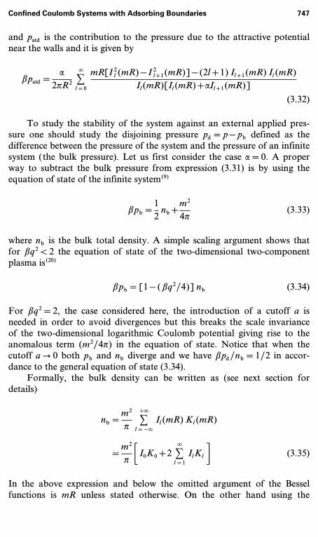
and patd is the contribution to the pressure due to the attractive potentialnear the walls and it is given by

bpatd=a

2pR2 C.

l=0

mR[I2l (mR) − I2

l+1(mR)] − (2l+1) Il+1(mR) Il(mR)Il(mR)[Il(mR)+aIl+1(mR)]

(3.32)

To study the stability of the system against an external applied pres-sure one should study the disjoining pressure pd=p − pb defined as thedifference between the pressure of the system and the pressure of an infinitesystem (the bulk pressure). Let us first consider the case a=0. A properway to subtract the bulk pressure from expression (3.31) is by using theequation of state of the infinite system (9)

bpb=12

nb+m2

4p(3.33)

where nb is the bulk total density. A simple scaling argument shows thatfor bq2 < 2 the equation of state of the two-dimensional two-componentplasma is (20)

bpb=[1 − (bq2/4)] nb (3.34)

For bq2=2, the case considered here, the introduction of a cutoff a isneeded in order to avoid divergences but this breaks the scale invarianceof the two-dimensional logarithmic Coulomb potential giving rise to theanomalous term (m2/4p) in the equation of state. Notice that when thecutoff a Q 0 both pb and nb diverge and we have bpd/nb=1/2 in accor-dance to the general equation of state (3.34).

Formally, the bulk density can be written as (see next section fordetails)

nb=m2

pC+.

l=−.

Il(mR) Kl(mR)

=m2

p5I0K0+2 C

.

l=1IlKl

6 (3.35)

In the above expression and below the omitted argument of the Besselfunctions is mR unless stated otherwise. On the other hand using the


Wronskian (21) IlKl+1+Il+1Kl=(1/mR) the hard disk pressure (3.31) canbe formally written as

bphd=m2

p5 C

.

l=0

I2l+1Kl

Il+ C

.

l=1IlKl

6 (3.36)

Then the disjoining pressure for a=0 is given by

b(phd − pb)=bphd, disj=m2

p5 C

.

l=0

I2l+1Kl

Il−

I0K0

2−

146 (3.37)

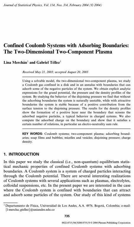
Although the pressure phd and the bulk pressure pb are divergent when thecutoff a vanishes, the disjoining pressure phd, disj in the case a=0 proves tobe well-defined for a Q 0 and the series (3.37) is convergent.

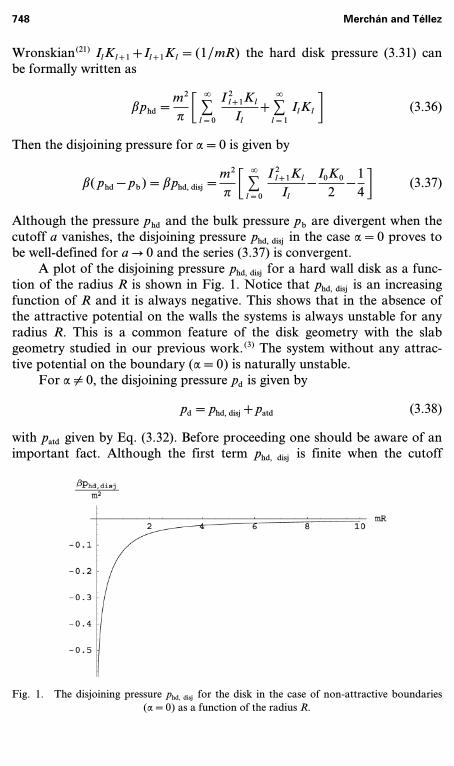
A plot of the disjoining pressure phd, disj for a hard wall disk as a func-tion of the radius R is shown in Fig. 1. Notice that phd, disj is an increasingfunction of R and it is always negative. This shows that in the absence ofthe attractive potential on the walls the systems is always unstable for anyradius R. This is a common feature of the disk geometry with the slabgeometry studied in our previous work. (3) The system without any attrac-tive potential on the boundary (a=0) is naturally unstable.

For a ] 0, the disjoining pressure pd is given by

pd=phd, disj+patd (3.38)

with patd given by Eq. (3.32). Before proceeding one should be aware of animportant fact. Although the first term phd, disj is finite when the cutoff

Fig. 1. The disjoining pressure phd, disj for the disk in the case of non-attractive boundaries(a=0) as a function of the radius R.


a Q 0 the second term on the other hand is divergent when a Q 0. The sumin Eq. (3.32) should be cutoff to a upper limit N=R/a as it was done inthe preceding section. Rigorously speaking when a Q 0 the dominant termfor the disjoining pressure is patd. For large radius R, from last sectionresults (3.22) and (3.28) on the finite-size corrections we can deduce thedominant term of the disjoining pressure when a Q 0

bpd ’ −1R

bc

’am4pR

ln2

ma(3.39)

This term is always positive and is a decreasing function of R indicatingthat the system is always stable.

This is an important difference between the slab geometry studied inref. 3 and the present case of the disk. In the slab geometry the disjoiningpressure is always finite for a=0 and any value of a. For a slab of width W,the large-W expansion of the grand potential per unit area w reads (3)

w=−pbW+2c+O(e−mW) (3.40)

Then the pressure p=“w/“W does not contain any contribution from thesurface tension. On the other hand in the disk geometry considered herethe existence of the curvature makes the surface tension c very relevant forthe disjoining pressure (see Eq. (3.39)) and since c diverges logarithmicallywith the cutoff it plays a dominant role in the stability of the system.

Let us now consider a small but non-zero cutoff a. It is expected thatthe results of our theory in that case should be close to the ones of amodel of small hard-core particles of diameter a. Then there will be acompetition between the natural unstable behavior of the case withoutattractive potential (a=0) and the attractive part to the pressure patd

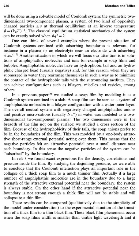
which is stabilizing.Figure 2 shows several plots of the disjoining pressure pd as a function

of the radius R for three special values of the adhesivity a=0.15, 0.21, and0.3 for a fixed cutoff ma=10−3. These three plots show three characteristicregimes in which the system can be.

For large values of the adhesivity, for example the case a=0.3 shownin Fig. 2, the disjoining pressure is always positive and a decreasing func-tion of the radius R. The system is stable for all values of the radius R.

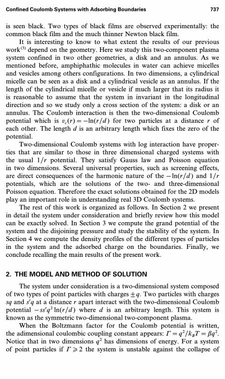
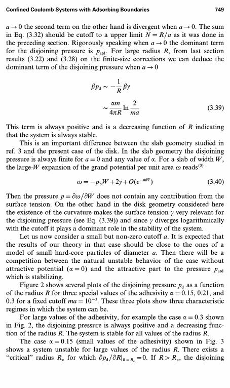
The case a=0.15 (small values of the adhesivity) shown in Fig. 3shows a system unstable for large values of the radius R. There exists a‘‘critical’’ radius Rc for which “pd/“R|R=Rc

=0. If R > Rc, the disjoining


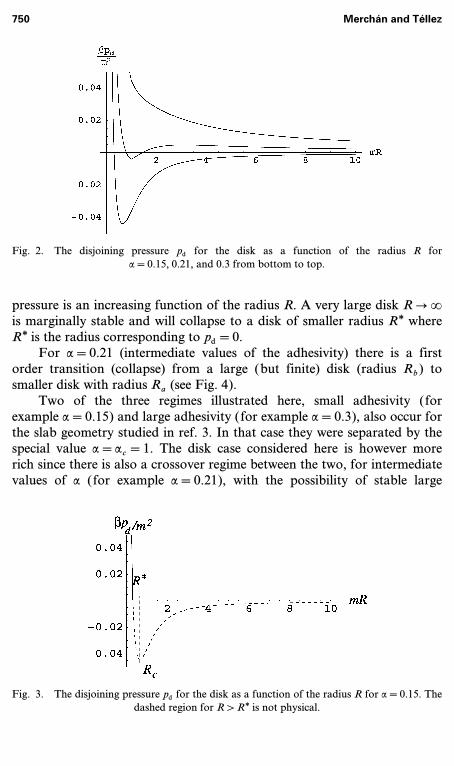
Fig. 2. The disjoining pressure pd for the disk as a function of the radius R fora=0.15, 0.21, and 0.3 from bottom to top.

pressure is an increasing function of the radius R. A very large disk R Q .

is marginally stable and will collapse to a disk of smaller radius Rg whereRg is the radius corresponding to pd=0.

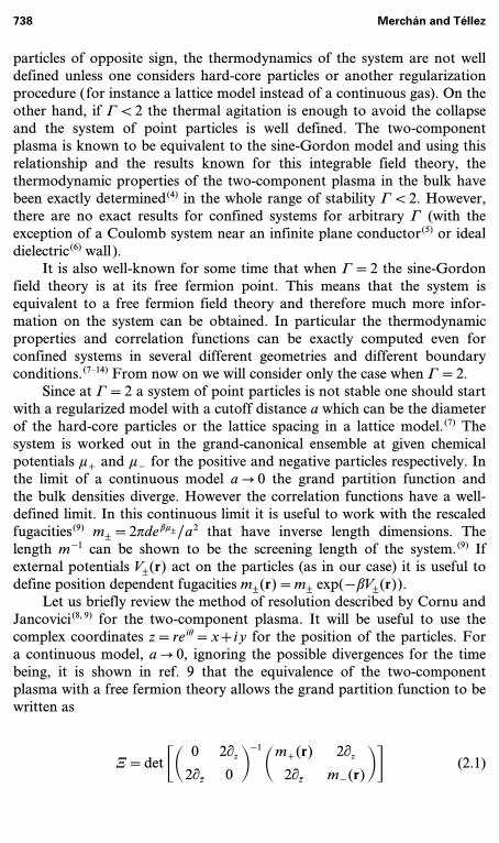
For a=0.21 (intermediate values of the adhesivity) there is a firstorder transition (collapse) from a large (but finite) disk (radius Rb ) tosmaller disk with radius Ra (see Fig. 4).

Two of the three regimes illustrated here, small adhesivity (forexample a=0.15) and large adhesivity (for example a=0.3), also occur forthe slab geometry studied in ref. 3. In that case they were separated by thespecial value a=ac=1. The disk case considered here is however morerich since there is also a crossover regime between the two, for intermediatevalues of a (for example a=0.21), with the possibility of stable large

Fig. 3. The disjoining pressure pd for the disk as a function of the radius R for a=0.15. Thedashed region for R > Rg is not physical.


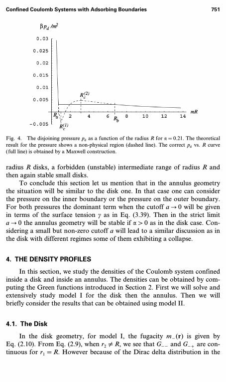
Fig. 4. The disjoining pressure pd as a function of the radius R for a=0.21. The theoreticalresult for the pressure shows a non-physical region (dashed line). The correct pd vs. R curve(full line) is obtained by a Maxwell construction.

radius R disks, a forbidden (unstable) intermediate range of radius R andthen again stable small disks.

To conclude this section let us mention that in the annulus geometrythe situation will be similar to the disk one. In that case one can considerthe pressure on the inner boundary or the pressure on the outer boundary.For both pressures the dominant term when the cutoff a Q 0 will be givenin terms of the surface tension c as in Eq. (3.39). Then in the strict limita Q 0 the annulus geometry will be stable if a > 0 as in the disk case. Con-sidering a small but non-zero cutoff a will lead to a similar discussion as inthe disk with different regimes some of them exhibiting a collapse.

4. THE DENSITY PROFILES

In this section, we study the densities of the Coulomb system confinedinside a disk and inside an annulus. The densities can be obtained by com-puting the Green functions introduced in Section 2. First we will solve andextensively study model I for the disk then the annulus. Then we willbriefly consider the results that can be obtained using model II.

4.1. The Disk

In the disk geometry, for model I, the fugacity m− (r) is given byEq. (2.10). From Eq. (2.9), when r2 ] R, we see that G− − and G−+ are con-tinuous for r1=R. However because of the Dirac delta distribution in the


definition of m− (r) the functions G+− and G++ are discontinuous at r1=R.The discontinuity can be obtained from Eq. (2.9) if r2 ] r1:

G++ (r1=R−, r2) − G++ (r1=R+, r2)=ae−ih1G− + (r1=R, r2) (4.1)

If both points r1 and r2 are inside the disk but not on the boundarythen Eq. (2.9) lead to a Helmoltz equation for G++ and for G− −

[m2 − D] G± ±(r1, r2)=md(r1 − r2) (4.2)

and the other Green functions can be obtained from

e ± ih1

m1 − “r1

+ir1

“h12 G± ±(r1, r2)=G+ ± (r1, r2) (4.3)

If r1 is outside the film while r2 is fixed inside the film m+(r1)=m− (r1)=0, the Gs1 s2

that satisfy Eq. (2.9) are

G++ (r1, r2)= C+.

l=−.

Cl(r2, h2)(r1e ih1) l (4.4)

G− + (r1, r2)= C+.

l=−.

Dl(r2, h2)(r1e−ih1)−l (4.5)

So, in order to have finite solutions at r1=. it is necessary that for r1 > R

Cl(r2, h2)=0 for l \ 0

Dl(r2, h2)=0 for l [ 0(4.6)

Eqs. (4.1) and (4.6) are the boundary conditions that complement the dif-ferential equations (4.2) and (4.3) for the Green functions.

Solving Eq. (4.2), we arrive to the following expressions for the Greenfunctions for 0 [ r1, 2 < R:

G++(r1, r2)=m2p

K0(m |r1 − r2 |)

+m2p

C+.

l=0e il(h1 − h2 ) 5Kl

IlIl+1(mr1) Il+1(mr2)

+aKl+1 − Kl

aIl+1+IlIl(mr1) Il(mr2)6 (4.7)


and

G− − (r1, r2)=m2p

K0(m |r1 − r2 |)

−m2p

C+.

l=0e il(h1 − h2 ) 5Kl

IlIl(mr1) Il(mr2)

+aKl+1 − Kl

aIl+1+IlIl+1(mr1) Il+1(mr2)6 (4.8)

with Il meaning Il(mR) and the same convention for the Bessel function Kl.The one-particle densities are given in terms of these Green functions

as rs(r)=ms(r) Gss(r, r). As we explained in Section 2 the continuous limitmodel presents divergences in the expressions of the densities. This is seenin the term K0(mr12) that diverges logarithmically as r12=|r1 − r2 | Q 0. Sowe impose a short distance cutoff a. One can think that particles are disksof diameter a, so the minimal distance between particles is a.

The first term in Eqs. (4.7) and (4.8) gives the bulk density rb, thedensity of the unbounded system as calculated in ref. 9. For a Q 0

r+b =r−

b =rb=m2

2pK0(ma) ’

m2

2p5ln

2ma

− c6 (4.9)

where c 4 0.5772 is the Euler constant. In the second terms of Eqs. (4.7)and (4.8) the sum can eventually diverge when r1=r2=r for certain valuesof r (in the boundaries) so we should impose a cutoff |l| < N=R/a asit has been done in the expressions of the pressure and grand-potentialobtained in the last section.

Because of the form (2.10) of m− (r), the negative density can bewritten as

r− (r)=11+a

md(r − R)2 rg

− (r) (4.10)

where rg− can be seen as the density of non-adsorbed particles. For the

positive particles r+=rg+. Finally we have

rg+(r)=rb+

m2

2pC.

l=0

5Kl

IlI2

l+1(mr)+aKl+1 − Kl

aIl+1+IlI2

l (mr)6 (4.11a)

rg− (r)=rb −

m2

2pC.

l=0

5Kl

IlI2

l (mr)+aKl+1 − Kl

aIl+1+IlI2

l+1(mr)6 (4.11b)


The non-adsorbed charge density rg=rg+ − rg

− can be obtained fromthe above expression and using the Wronskian of the Bessel functionsIlKl+1+Il+1Kl=1/mR,

rg(r)=am2

2pRC.

l=0

I2l+1(mr)+I2

l (mr)(aIl+1+Il) Il

(4.12)

Finally, the total charge density

r(r)=r+(r) − r− (r)

=r+(r) −11+a

md(r − R)2 rg

− (r)

=rg(r) − s− d(r − R) (4.13)

has a non-adsorbed part rg(r) and a adsorbed ‘‘surface’’ charge density inthe boundary

s− =a

mrg

− (R) (4.14)

This surface charge density s− comes from the d(r − R) part of the negativecharge density. Writing formally the bulk part of the density as rb=(m2/2p) ;l ¥ Z IlKl one can obtain the following expression for s− fromEqs. (4.14) and (4.11b)

s− =a

2pRC.

l=0

Il+1

aIl+1+Il(4.15)

Actually the adsorbed charge density should obey two special rela-tions. The first is a sum rule that expresses the global electro-neutrality ofthe system

R s− =FR

0rg(r) r dr (4.16)

Using a known indefinite integral (21) for products of Bessel functions, thissum rule (4.16) is immediately shown to be satisfied.

On the other hand the adhesivity a can be thought as a sort of fugacitythat controls the number of adsorbed particles (1) and one can obtain the


total number of adsorbed particles 2pRs− from the grand potential W byusing the usual thermodynamic relation

2pR s− =−ab“W

“a(4.17)

This relationship is also immediately shown to be satisfied from theexpression (3.12) for WD

at, the part of the grand potential that depends on a.For a large disk, R Q ., the dominant part of the grand potential that

depends on a is the surface tension c given by Eqs. (3.23) and (3.28). Thenwe have

s− =−ba“c

“a(4.18)

a relation already shown to be true in ref. 3 for the same system near aplane attractive hard wall. Using Eq. (3.23) into Eq. (4.18) gives explicitly

s− =m4p

5a ln2

ma−

a2+1a

ln(a+1)+16 (4.19)

Thus recovering a known result from ref. 3. This result can, of course, alsobe obtained directly from Eq. (4.15) in the limit of large-R using the Debyeexpansions (3.20) of the Bessel functions.

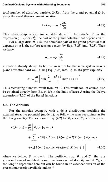
4.2. The Annulus

For the annulus geometry with a delta distribution modeling theexternal attractive potential (model I), we follow the same reasonings as forthe disk geometry. The solution to Eq. (4.2) for R1 < r < R2 is of the form

Gss(r1, r2)=m2p

5K0(m |r1 − r2 |)

+ C+.

l=−.

e ilh12[AlIl(mr1) Il(mr2)+BlKl(mr1) Kl(mr2)

+Cl[Il(mr1) Kl(mr2)+Il(mr2) Kl(mr1)]]6 (4.20)

where we defined h12=h1 − h2. The coefficients Al, Bl, and Cl, that aregiven in terms of modified Bessel functions evaluated at R1 and at R2, aretoo long to reproduce here but can be found in an extended version of thepresent manuscript available online. (23)


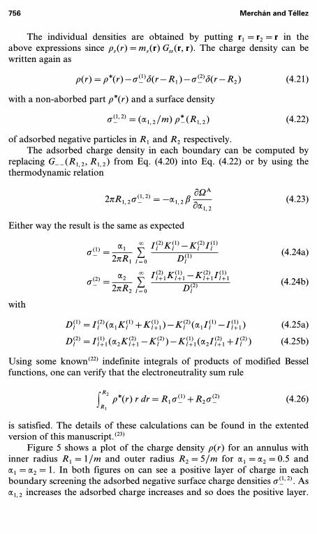
The individual densities are obtained by putting r1=r2=r in theabove expressions since rs(r)=ms(r) Gss(r, r). The charge density can bewritten again as

r(r)=rg(r) − s (1)− d(r − R1) − s (2)

− d(r − R2) (4.21)

with a non-aborbed part rg(r) and a surface density

s (1, 2)− =(a1, 2/m) rg

− (R1, 2) (4.22)

of adsorbed negative particles in R1 and R2 respectively.The adsorbed charge density in each boundary can be computed by

replacing G− − (R1, 2, R1, 2) from Eq. (4.20) into Eq. (4.22) or by using thethermodynamic relation

2pR1, 2 s (1, 2)− =−a1, 2 b

“WA

“a1, 2(4.23)

Either way the result is the same as expected

s (1)− =

a1

2pR1C.

l=0

I (2)l K (1)

l − K (2)l I (1)

l

D (1)l

(4.24a)

s (2)− =

a2

2pR2C.

l=0

I (2)l+1K (1)

l+1 − K (2)l+1I (1)

l+1

D (2)l

(4.24b)

with

D (1)l =I (2)

l (a1K (1)l +K(1)

l+1) − K (2)l (a1I (1)

l − I (1)l+1) (4.25a)

D (2)l =I (1)

l+1(a2K (2)l+1 − K (2)

l ) − K (1)l+1(a2I (2)

l+1+I(2)l ) (4.25b)

Using some known (22) indefinite integrals of products of modified Besselfunctions, one can verify that the electroneutrality sum rule

FR2

R1

rg(r) r dr=R1 s (1)− +R2 s (2)

− (4.26)

is satisfied. The details of these calculations can be found in the extentedversion of this manuscript. (23)

Figure 5 shows a plot of the charge density r(r) for an annulus withinner radius R1=1/m and outer radius R2=5/m for a1=a2=0.5 anda1=a2=1. In both figures on can see a positive layer of charge in eachboundary screening the adsorbed negative surface charge densities s (1, 2)

− . Asa1, 2 increases the adsorbed charge increases and so does the positive layer.


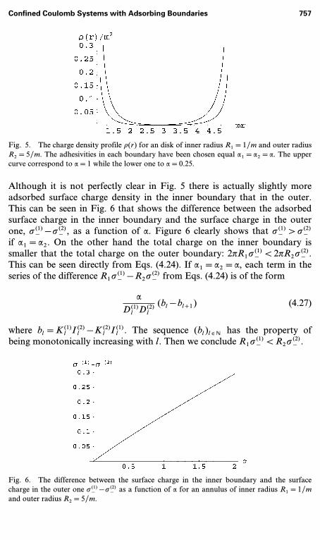
Fig. 5. The charge density profile r(r) for an disk of inner radius R1=1/m and outer radiusR2=5/m. The adhesivities in each boundary have been chosen equal a1=a2=a. The uppercurve correspond to a=1 while the lower one to a=0.25.

Although it is not perfectly clear in Fig. 5 there is actually slightly moreadsorbed surface charge density in the inner boundary that in the outer.This can be seen in Fig. 6 that shows the difference between the adsorbedsurface charge in the inner boundary and the surface charge in the outerone, s (1)

− − s (2)− , as a function of a. Figure 6 clearly shows that s (1)

− > s (2)−

if a1=a2. On the other hand the total charge on the inner boundary issmaller that the total charge on the outer boundary: 2pR1 s (1)

− < 2pR2 s (2)− .

This can be seen directly from Eqs. (4.24). If a1=a2=a, each term in theseries of the difference R1 s (1)

− − R2 s (2)− from Eqs. (4.24) is of the form

a

D (1)l D (2)

l

(bl − bl+1) (4.27)

where bl=K(1)l I (2)

l − K (2)l I (1)

l . The sequence (bl)l ¥ N has the property ofbeing monotonically increasing with l. Then we conclude R1 s (1)

− < R2 s (2)− .

Fig. 6. The difference between the surface charge in the inner boundary and the surfacecharge in the outer one s (1)

− − s (2)− as a function of a for an annulus of inner radius R1=1/m

and outer radius R2=5/m.


4.3. Model II

We now briefly consider model II and some of its results in theannulus geometry. In model II, we can distinguish three regions: the innerborder R1 < r1 < R1+D (region 1), the bulk of the film R1+D < r1 <R2 − D (region 2) and the outer border R2 − D < r1 < R2 (region 3). Wedefine the position dependent fugacities as

m+(r1)=m, in all regions 1, 2, and 3 (4.28a)

m− (r1)=˛m2 if r1 ¥ region 1

m if r1 ¥ region 2

m2 if r1 ¥ region 3

(4.28b)

The fugacity in the border regions is m2=m exp(−bU− ) where U− < 0is the value of the external potential V− (r) near the boundary. Notice thatm2 > m. It is clear that model I is the limit of model II when D Q 0 andm2 Q . with the product m2D=a finite.

For this model II, it is useful to use a symmetrization procedureexplained in ref. 9. Using this procedure it turns out that in regions 1 and 3the important parameter is m0=(mm2)1/2 instead of the individual fugacities.

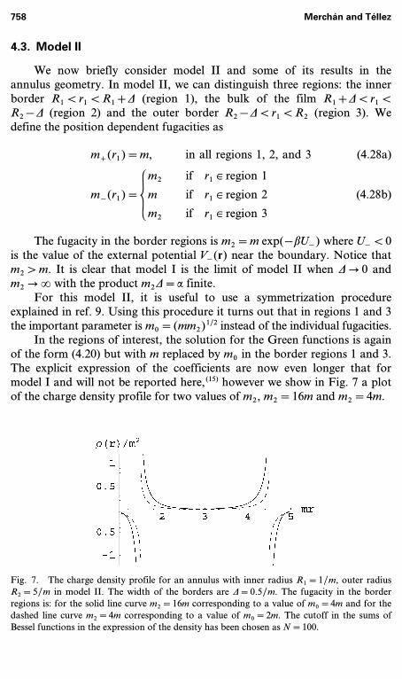
In the regions of interest, the solution for the Green functions is againof the form (4.20) but with m replaced by m0 in the border regions 1 and 3.The explicit expression of the coefficients are now even longer that formodel I and will not be reported here, (15) however we show in Fig. 7 a plotof the charge density profile for two values of m2, m2=16m and m2=4m.

Fig. 7. The charge density profile for an annulus with inner radius R1=1/m, outer radiusR2=5/m in model II. The width of the borders are D=0.5/m. The fugacity in the borderregions is: for the solid line curve m2=16m corresponding to a value of m0=4m and for thedashed line curve m2=4m corresponding to a value of m0=2m. The cutoff in the sums ofBessel functions in the expression of the density has been chosen as N=100.


The discontinuity of the charge density profile near the interfaces isdue to the fact that the density profile of the negative particles is discon-tinuous there. This is expected for the negative particles since the potentialV− (r) is discontinuous across the interfaces. In general for a fluid withdensity n(x) near a planar interface characterized by an external potentialVext(x) eventually discontinuous at x=0 the y-function exp(bVext(x)) n(x)is continuous. (24)

There is a higher density of particles (both negative and positive) inthe borders that in the bulk: for higher values of the fugacity m2 in theborder (the external potential V− (r) is more attractive), the density in theborders is higher. In region 2, the density far from the interfaces is close tothe bulk value (4.9). In the borders, away from the interfaces both densitiesr+(r) and r− (r) try to be close to the new bulk value given by Eq. (4.9)replacing m by m0. Due to the natural tendency of the system to be electri-cally neutral, the positive particles try to follow the negative ones so thesystem is not locally charged. However at the interfaces r=R1+D andr=R2 − D there remains a non-neutral charge density that can be seen inFig. 7. Actually one can see in Fig. 7 a double charged layer. Inside theborder region (1 or 3) there is a negative charge density layer and outsidethe border, in the bulk region 2, a positive layer, the same one that waspreviously observed with model I in Fig. 5. These double layers have athickness of order m−1 for the positive layer in region 2 and m−1

0 for thenegative layer in regions 1 and 3.

5. SUMMARY AND PERSPECTIVES

The present solvable model studied here gave us interesting informa-tion about the behavior of confined Coulomb systems with attractiveboundaries. This system has an induced internal charge on the boundarywhich is created by an external potential which is not of electrical nature.This potential only acts on the negative particles, while the positive par-ticles are unaffected. This is not the usual situation that has been studiedextensively in the past, where the system is submitted to electrical forcesdue to possible external charges.

First, we found that large systems exhibit the same finite-size correc-tions that for systems without attractive boundaries, confirming again theuniversal nature of these finite-size corrections. Studying the disjoiningpressure we found that the attractive boundaries have a stabilizing effect.This was noticed also in our previous work, (3) however the curvature in thepresent case is very important. It makes the surface tension to be the pre-dominant contribution to the disjoining pressure, as opposed to the slabgeometry. Then, we conclude that the curvature has also a stabilizing effect


on the system in comparison to the slab geometry in which the system canbe unstable for low values of the adhesivity.

The study of the density profiles gives information about the structureof the system. As expected, there are some adsorbed charges on theboundary and these are screened by a positive layer of charge inside thesystem. We were able to check explicitly an electro-neutrality sum rule anda few relations that the adsorbed charge in the boundary satisfy.

It would be interesting to know what features of the present model areuniversal and which are not. A step toward answering this question can beobtained by studying another solvable model of Coulomb system, the one-component plasma. A preliminary study of this system was done in ref. 15and this will be the subject of a future paper.

ACKNOWLEDGMENTS

The authors would like to thank the following agencies for theirfinancial support: ECOS-Nord (France), COLCIENCIAS-ICFES-ICETEX(Colombia), Banco de la República (Colombia), and Fondo de Investiga-ciones de la Facultad de Ciencias de la Universidad de los Andes(Colombia).

REFERENCES

1. M. L. Rosinberg, J. L. Lebowitz, and L. Blum, A solvable model for localized adsorptionin a Coulomb system, J. Stat. Phys. 44:153–182 (1986).

2. F. Cornu, Two-dimensional models for an electrode with adsorption sites, J. Stat. Phys.54:681–706 (1989).

3. G. Téllez and L. Merchán, Solvable model for electrolytic soap films: The two-dimen-sional two-component plasma, J. Stat. Phys. 108:495–525 (2002).

4. L. Samaj and I. Travenec, Thermodynamic properties of the two-dimensional two-com-ponent plasma, J. Stat. Phys. 101:713–730 (2000).

5. L. Samaj and B. Jancovici, Surface tension of a metal-electrolyte boundary: Exactly solv-able model, J. Stat. Phys. 103:717–735 (2001).

6. L. Samaj, Surface tension of an ideal dielectric-electrolyte boundary: Exactly solvablemodel, J. Stat. Phys. 103:737–752 (2001).

7. M. Gaudin, L’isotherme critique d’un plasma sur réseau (b=2, d=2, n=2), J. Physique(France) 46:1027–1042 (1985).

8. F. Cornu and B. Jancovici, On the two-dimensional Coulomb gas, J. Stat. Phys. 49:33–56(1987).

9. F. Cornu and B. Jancovici, The electrical double layer: A solvable model, J. Chem. Phys.90:2444–2452 (1989).

10. P. J. Forrester, Density and correlation functions for the two-component plasma at C=2near a metal wall, J. Chem. Phys. 95:4545–4549 (1991).

11. B. Jancovici, G. Manificat, and C. Pisani, Coulomb systems seen as critical systems: Finite-size effects in two dimensions, J. Stat. Phys. 76:307–329 (1994).


12. B. Jancovici and G. Téllez, Coulomb systems seen as critical systems: Ideal conductorboundaries, J. Stat. Phys. 82:609–632 (1996).

13. B. Jancovici and L. Samaj, Coulomb systems with ideal dielectric boundaries: Freefermion point and universality, J. Stat. Phys. 104:753–775 (2001).

14. G. Téllez, Two-dimensional coulomb systems in a disk with ideal dielectric boundaries,J. Stat. Phys. 104:945–970 (2001).

15. L. Merchán, Two-Dimensional Coulomb Systems in a Confined Geometry Subject to anAttractive Potential on the Boundary, Master Thesis (Universidad de los Andes, Bogotá,2003).

16. P. J. Forrester, Surface tension for the two-component plasma at C=2 near an interface,J. Stat. Phys. 67:433–448 (1992).

17. J. L. Cardy and I. Peschel, Finite-size dependence of the free energy in two-dimensionalcritical systems, Nuclear Phys. B 300:377–392 (1988).

18. J. L. Cardy, in Fields, Strings, and Critical Phenomena, Les Houches 1988, E. Brézin andJ. Zinn-Justin, eds. (North-Holland, Amsterdam, 1990).

19. M. Abramowitz and I. A. Stegun, Handbook of Mathematical Functions (National Bureauof Standards, Washington, D.C., 1964).

20. E. H. Hauge and P. C. Hemmer, Phys. Norv. 5:209 (1971).21. S. Gradshteyn and I. M. Ryzhik, Table of Integrals, Series, and Products (Academic, New

York, 1965).22. G. N. Watson, A Treatise on the Theory of Bessel Functions (Cambridge University Press,

United Kingdom, 1922).23. L. Merchán and G. Téllez, Confined Coulomb Systems with Absorbing Boundaries: The

Two-Dimensional Two-Component Plasma, version 1, http://arXiv.org/abs/cond-mat/0305514v1 (2003).

24. J. R. Henderson, in Fundamentals of Inhomogeneous Fluids, Chap. 2, D. Henderson, ed.(Dekker, New York, 1992).


Documents

Confined Coulomb systems with adsorbing boundaries: the two-dimensional two-component plasma