Embed Size (px)
Citation preview
LICENTIATE THESIS
Department of Applied Physics and Mechanical EngineeringDivision of Computer Aided Design
2004:04 • ISSN: 1402 - 1757 • ISRN: LTU - LIC - - 04/04 - - SE
2004:04
Constrained Optimization of Rotor-Bearing Systems by Evolutionary Algorithms
ANDERS ANGANTYR
Universitetstryckeriet, Luleå

ii
iii
Preface The work with this thesis has been carried out at the Division of Computer Aided Design, Luleå University of Technology. This project has to a large extent been funded by Demag Delaval Industrial Turbomachinery AB*. I therefore would like to acknowledge the company for the sponsoring of the project. The first person to thank is my supervisor PhD Jan-Olov Aidanpää who recruited me to the academic world during the under graduate studies. To supervise persistent student is not always easy I suppose. However, Jan-Olov has done a terrific job when leading me into the research, then guided me and now and then helped me to find the track. Secondly I would like to thank Professor Thommy Karlsson who originally initiated the project and has served as a mentor during the graduate studies. Tech. Lic. Per Nilsson also made extensive efforts in the startup phase of the project and therefore deserves a special thanks. My co-author of Paper B PhD Johan Andersson§ has been an important person in the parts of the project that concerns the search and optimization theory. I greatly appreciate the discussions about evolutionary optimization and the feedback given in this field. The involved staff at Demag Delaval Industrial Turbomachinery AB deserves an acknowledgement for the smooth cooperation and help with the practical problems. A special thanks is directed to Bo Hagstedt who has been an important support for problems concerning the computer codes and for introducing me to Python. Last but not least, I would like to thank my colleges at the division for the relaxed atmosphere and interesting discussions during the coffee breaks around the table in the Polhem Laboratory. Luleå, January 2004 Anders Angantyr
* Name of company 14/01/2004 Visiting Professor at the Division of Computer Aided Design and employed by SwedPower Currently at ABB § Linköping University

iv
v
Abstract In the design of mechanical components and systems, nature has often been the source of inspiration. It is easy to point out solutions in nature that are optimal in some sense. One example is the roughness of the surface of a sharks skin. This is designed by nature to minimize the resistance when the shark swims in the water. Another example is the shape of an egg shell. This is an optimal load carrying structure which is often found in engineering design applications. An even more fascinating question is how nature has found these optimal solutions? The answer to this question is evolution. Instead of just analyzing and copying optimal structures invented by nature it seems reasonable to mimic the process how nature has came up with these solutions. Research on how these ideas can be interpreted and used in engineering design started in the early seventies and has now become a large field known as Evolutionary Algorithms (EAs). During the past decade these methods have emerged as potent tools for engineering design optimization. Some of these methods are especially suited for problems which involve multiple objectives such as almost all real engineering design problems. Just until recently, these methods have seldom been used in the area of rotordynamical design. This thesis deals with the question how these methods can be adapted and applied in order to improve the design and design process of large rotor-bearing system. A hypothesis for this work is that EAs are suitable to use in the late design process of these systems. The aim of this work is to evaluate this hypothesis by studying real applications found in industry. This thesis comprises an introductory part and four appended papers. The introductory part is divided into three different sections. In the first section the concept of engineering design optimization is introduced. In the second part Genetic Algorithms (GAs) is presented. Finally, the analysis and design of rotor-bearing systems are discussed in more general terms. The purpose with the introductory part is to introduce and prepare the reader to the concepts discussed in the papers. The introductory part may serve as a start point for newcomers interested in these areas. This overview is also the most important contribution of the introductory part of the thesis. The appended papers cover selected problems of constrained rotor-bearing system optimizations. In Paper A the multiobjective optimization of a generator is presented and discussed. Paper B introduces a constraint handling technique based on concepts found in multiobjective GAs. In Paper C and D this techniques is used for two different rotor-bearing system optimization problems where the actual geometry parameters of the bearings are used as design variables. Real rotor-bearing system design problems are constrained. A situation that occurs frequently is that a designer searches for solutions that are feasible with respect to some design constraints. In this thesis a generic constraint handling method for GAs is introduced. The result shows that it is robust and works for the studied cases. Another fact which has become apparent from the experiences of this work is that the problem formulation is important. The approaches used in this thesis are applicable in the late design stage or in the context of service and retrofit applications of rotor-bearing systems. This since the design problems in these cases have manageable magnitudes and are reasonably computationally expensive.

vi
vii
Thesis This thesis comprises an introductory part and four appended papers.
Paper A Angantyr, A. and Aidanpää, J-O., 2003, A Pareto Based Genetic Algorithm Search Approach to Handle Damped Natural Frequency Constraints in Turbo Generator Rotor System Design, Accepted for publication in ASME Journal of Engineering for Gas Turbines and Power.
Paper B Angantyr, A., Andersson, J. and Aidanpää, J-O., 2003, Constrained Optimization based on a Multiobjective Evolutionary Algorithm, In Sarker R. et al. (Eds.), Proceedings of the Congress on Evolutionary Computation, Canberra, Australia, IEEE-Press, 3, pp. 1560-1567.
Paper C Angantyr, A. and Aidanpää, J-O., 2004, Optimization of a Rotor-Bearing System with an Evolutionary Algorithm, Accepted for presentation at The 10th International Symposium on Rotating Machinery, March 7-11, Honolulu, Hawaii.
Paper D Angantyr, A. and Aidanpää, J-O., 2004, Constrained Optimization of Gas Turbine Tilting Pad Bearing Designs, To be submitted.

viii
ix
Contents 1 INTRODUCTION ...................................................................................................1
1.1 BACKGROUND ....................................................................................................1 1.2 RESEARCH QUESTION .........................................................................................2 1.3 AIM AND SCOPE OF RESEARCH............................................................................3 1.4 INDUSTRIAL AND ACADEMIC RELEVANCE...........................................................3
2 ENGINEERING DESIGN OPTIMIZATION ......................................................4 2.1 AN INTRODUCTORY TAPERED BEAM DESIGN EXAMPLE.......................................4 2.2 THE OPTIMIZATION PROBLEM.............................................................................5
2.2.1 The constrained single objective problem .................................................6 2.2.2 The multiobjective problem .......................................................................6
2.3 PRACTICAL ASPECTS OF ENGINEERING DESIGN OPTIMIZATION ...........................7 2.4 SOME OPTIMIZATION METHODS ..........................................................................9 2.5 EVOLUTIONARY ALGORITHMS..........................................................................10
2.5.1 Historical perspective..............................................................................10 2.5.2 Why and when to use EAs?......................................................................11
3 GENETIC ALGORITHMS..................................................................................12 3.1 CODING OF DESIGN PROBLEM ...........................................................................12 3.2 THE POPULATION..............................................................................................13 3.3 EVOLUTION OF POPULATION.............................................................................13
3.3.1 Fitness assignment and ranking ..............................................................15 3.3.2 Selection ..................................................................................................16 3.3.3 Crossover.................................................................................................17 3.3.4 Mutation ..................................................................................................18 3.3.5 Reinsertion...............................................................................................19
3.4 MULTIOBJECTIVE GAS.....................................................................................19 3.5 CONSTRAINT HANDLING...................................................................................21 3.6 SOME REMARKS ON GAS..................................................................................22
4 ROTOR-BEARING SYSTEM ANALYSIS AND DESIGN ..............................24 4.1 ROTORDYNAMIC ANALYSIS ..............................................................................24
4.1.1 Discretized rotor-bearing systems models (multi DOF models)..............24 4.1.2 Analysis by the state space approach ......................................................25 4.1.3 Gyroscopic effect and critical speeds ......................................................27 4.1.4 Effects of journal bearings.......................................................................30 4.1.5 Some special effects in rotordynamic analyses........................................33
4.2 DESIGN OF ROTOR-BEARING SYSTEMS..............................................................34 5 SUMMARY OF APPENDED PAPERS ..............................................................37
5.1 PAPER A...........................................................................................................37 5.2 PAPER B ...........................................................................................................37 5.3 PAPER C ...........................................................................................................38

x
xi
5.4 PAPER D...........................................................................................................38 5.5 AUTHORS CONTRIBUTION ...............................................................................39
6 DISCUSSION AND FUTURE WORK................................................................40 6.1 ANSWER TO RESEARCH QUESTIONS ..................................................................40 6.2 IMPORTANCE OF PROBLEM FORMULATION .......................................................40 6.3 FUTURE WORK..................................................................................................40
7 REFERENCES ......................................................................................................42 8 APPENDIX ............................................................................................................47
Appended papers Paper A A Pareto Based Genetic Algorithm Search Approach to Handle
Damped Natural Frequency Constraints in Turbo Generator Rotor System Design
Paper B Constrained Optimization based on a Multiobjective Evolutionary Algorithm
Paper C Optimization of a Rotor-Bearing System with an Evolutionary Algorithm
Paper D Constrained Optimization of Gas Turbine Tilting Pad Bearing Designs

xii
A. Angantyr Constrained Optimization of Rotor-Bearing Systems by Evolutionary Algorithms
1
1 Introduction The body of this thesis is an introduction to the subject for the research. This first section gives a background and defines the research in a wider manner. In the following section, the matter of engineering design optimization is introduced and discussed qualitatively. The third section gives a more detailed description of Genetic Algorithms (GAs) which is on class of Evolutionary Algorithms (EAs). Different types of real coded GAs have been used extensively during the work with this thesis. Then, the dynamical design and analysis of large rotor-bearing systems are dealt with. In this thesis, large rotor-bearing systems means gas turbines, turbo generators, etc, which usually are supported by hydrodynamic journal bearings. Finally, the appended papers are summarized and a discussion of the research so far is held. The authors aim with the outline of this thesis is that each section can be read independently depending of the readers interest and prior knowledge. A reader with no prior knowledge in the area of rotordynamics and EAs is encouraged to read all sections. This should give enough understanding in order to catch the concepts in the appended papers.
1.1 Background The design of high speed rotating machines started in the late 19th century by for example the cream separator by De Laval. In the early 20th century the development of the steam turbine started. During the 2nd world war the development of the turbo jet engine accelerated. Today there is no dramatic difference between a modern gas turbine for power production and a turbo jet engine from the 1950s. The most striking differences may be the efficiency and emission levels. Most of todays high speed rotating machines are based on concepts invented decades ago. This means that most of the development and design of these machines will only be small improvements of existing machines. Still this is important since even small improvements in performance of several MW machines may yield substantially increased profit. Perhaps even more important factors in the design of these machines are to reduce costs and increase reliability. The design process of large rotor-bearing systems of today is often an iterative refinement of known concepts. The detailed design process is definitely an iterative procedure or as Rajan et al. in [1] state The design of a rotor-bearing system is an iterative process in which the parameters that influence the design are modified until the desired design objectives are achieved. Apparently there is a potential to make use of optimization methods in the design process of rotor-bearing systems. Much work with optimization has been done of rotor systems supported by magnetic bearings. See for example [2] to [4] for further references. A rotor system with ball bearings was studied and optimized by Lee and Choi in [5]. In [6] Montusiewicz and Osyczka optimized a spindle supported by hydrostatic bearings. The eigenvalues of the system are often used as constraints or objectives in the optimization of rotor-bearing systems, [7] and [8]. An optimization with complex eigenvalue constraints and the mathematical model based on the state space approach is discussed by Chen and Wang in [9]. In [10] Shiau and Chang studied a rotor-bearing problem with multiple objectives. Various optimization methods have been known for decades. Still the use of optimization techniques in the practical design of rotor-bearing system is limited at
A. Angantyr Constrained Optimization of Rotor-Bearing Systems by Evolutionary Algorithms
2
industrial companies. An interesting question to pose is: Why is not optimization techniques used more frequently in industry? An obvious answer to this question is that it is seldom straight-forward to formulate optimization problems for real-world design problems where several objectives and constraints exist. It may be difficult to even distinguish the difference between objective and constraints. Another possible answer to the question is that most traditional optimization methods are not suitable for real-world problems with several non-linear objective functions and constraints that are difficult to satisfy. In the late 1960s ideas of search and optimization methods based on mechanisms found in natural evolution began to pop up. The natural evolution is slow, and so are most of these methods compared to many other optimization techniques. In the beginning, these methods did not receive much attention. But, due to the rapid development of computers it has now become practically possible to apply these methods on many different problem areas. The research about these methods has now become a large field itself. The main cause of this recover is that many difficult problems may be solved by these methods. In the next two sections, the background and use of EAs is described in some more detail. The ideas to use EAs or GAs in the field of rotordynamics are not new. An early application was [11] by Genta and Bassani. Later work with a variant of a GA was done by Choi and Yang, [12] and [13]. In [14] Choi and Yang studied the optimum placement of two eigenvalues for a rotor supported on hydrodynamic journal bearings with a GA. The bearing design parameters were not used as design variables. In [15] Choi and Yang optimized several objectives for a low pressure steam turbine with a weighted sum and a variant of a GA. The turbine was supported by hydrodynamic journal bearings and the bearing width and clearance was used as design variables but nothing was said about the actual bearing model. In most of the previously cited references, the mathematical models of the rotor-bearing systems are quite simple. This implies that the formulations of the optimization problems are relatively easy and straight-forward. For a designer working with more advanced models, several problems arise which not yet have been properly addressed. There will for example probably exist more objectives and constraints. The purpose of this work is to use analysis models with similar degree of complexity as used in industry and try to search for optimal solutions with respect to similar objectives and constraints as used in industry. The purpose is to evaluate and explore the possibilities to use EAs as search methods for this type of problems. It should be clear that validation and verification of the analysis models is important to get results that are close to the real behavior of the systems. This is however not the purpose for this work. In fact one may argue that the accuracy of the models affects how some of the constraints are set. Still the designer is left with a problem to push the design to the limiting conditions. Rotor-bearing system optimization problems are, as almost all real-world optimization problems, constrained. EAs have been criticized for the lack of robust and general constraint handling methods. This is also an area that this thesis should give some contributions to.
1.2 Research question A characteristic of a research project is that the current focus depends on the previously achieved results. In projects closely related to the industry, the focus will also change depending on the participants interest. The research question is therefore dynamic. It
A. Angantyr Constrained Optimization of Rotor-Bearing Systems by Evolutionary Algorithms
3
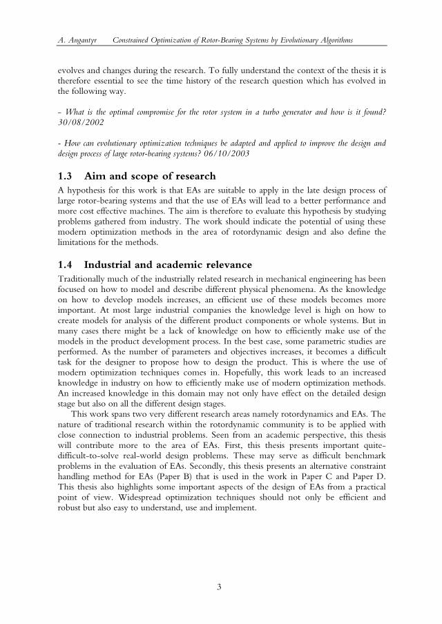
evolves and changes during the research. To fully understand the context of the thesis it is therefore essential to see the time history of the research question which has evolved in the following way. - What is the optimal compromise for the rotor system in a turbo generator and how is it found? 30/08/2002 - How can evolutionary optimization techniques be adapted and applied to improve the design and design process of large rotor-bearing systems? 06/10/2003
1.3 Aim and scope of research A hypothesis for this work is that EAs are suitable to apply in the late design process of large rotor-bearing systems and that the use of EAs will lead to a better performance and more cost effective machines. The aim is therefore to evaluate this hypothesis by studying problems gathered from industry. The work should indicate the potential of using these modern optimization methods in the area of rotordynamic design and also define the limitations for the methods.
1.4 Industrial and academic relevance Traditionally much of the industrially related research in mechanical engineering has been focused on how to model and describe different physical phenomena. As the knowledge on how to develop models increases, an efficient use of these models becomes more important. At most large industrial companies the knowledge level is high on how to create models for analysis of the different product components or whole systems. But in many cases there might be a lack of knowledge on how to efficiently make use of the models in the product development process. In the best case, some parametric studies are performed. As the number of parameters and objectives increases, it becomes a difficult task for the designer to propose how to design the product. This is where the use of modern optimization techniques comes in. Hopefully, this work leads to an increased knowledge in industry on how to efficiently make use of modern optimization methods. An increased knowledge in this domain may not only have effect on the detailed design stage but also on all the different design stages. This work spans two very different research areas namely rotordynamics and EAs. The nature of traditional research within the rotordynamic community is to be applied with close connection to industrial problems. Seen from an academic perspective, this thesis will contribute more to the area of EAs. First, this thesis presents important quite-difficult-to-solve real-world design problems. These may serve as difficult benchmark problems in the evaluation of EAs. Secondly, this thesis presents an alternative constraint handling method for EAs (Paper B) that is used in the work in Paper C and Paper D. This thesis also highlights some important aspects of the design of EAs from a practical point of view. Widespread optimization techniques should not only be efficient and robust but also easy to understand, use and implement.
A. Angantyr Constrained Optimization of Rotor-Bearing Systems by Evolutionary Algorithms
4
2 Engineering design optimization In this section the subject of engineering design optimization is introduced. The stand point is more from practical use of search and optimization methods than to start with rigorous mathematical proofs. First a simple example is introduced. Then the mathematical definition of some engineering design optimization problems is given. Finally some aspects of practical use of engineering design optimization are highlighted and some methods suitable to apply in many real-world problems are presented.
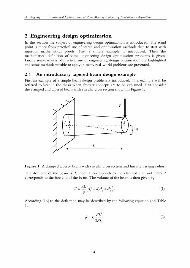
2.1 An introductory tapered beam design example First an example of a simple beam design problem is introduced. This example will be referred to later in the thesis when abstract concepts are to be explained. First consider the clamped and tapered beam with circular cross section shown in Figure 1.
Figure 1. A clamped tapered beam with circular cross section and linearly varying radius.
The diameter of the beam is d, index 1 corresponds to the clamped end and index 2 corresponds to the free end of the beam. The volume of the beam is then given by
( )2221
218
ddddLV ++=π . (1)
According [16] to the deflection may be described by the following equation and Table 1.
2
3
3EIPLk=δ (2)
P
δ
2 1
L
A. Angantyr Constrained Optimization of Rotor-Bearing Systems by Evolutionary Algorithms
5
The applied force (P) and length (L) are defined in Figure 1. E is Youngs modulus and I
is the area moment of inertia defined as 64
4dI π= . The multiplying factor k in equation
(2) is a function of the ratio of the area moment of inertia at the clamped end (I1) and the free end (I2) of the beam and given in Table 1.
Table 1. Multiplying factor k.
I1/I2 0.25 0.50 1.0 2.0 4.0 8.0 k 2.525 1.636 1.000 0.579 0.321 0.171
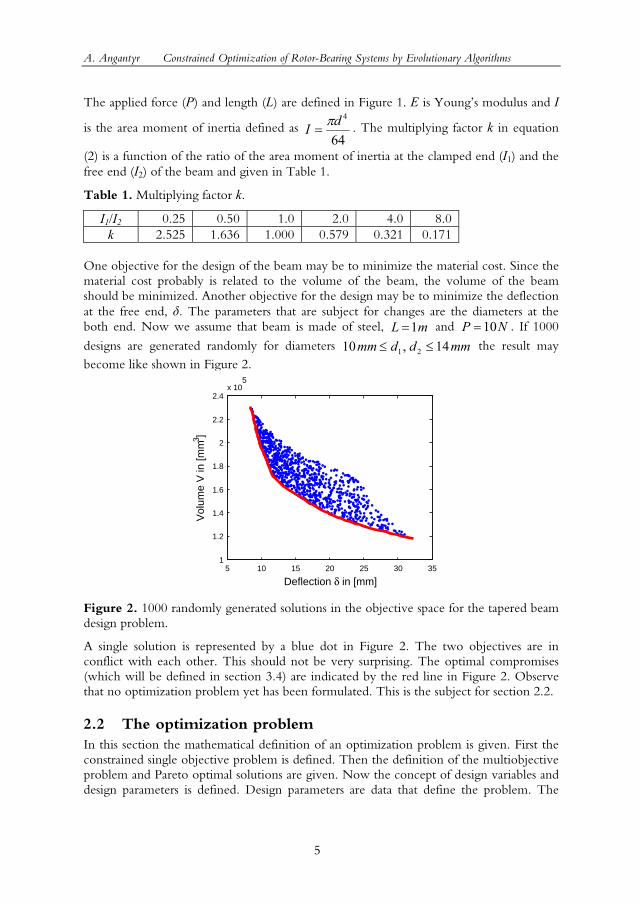
One objective for the design of the beam may be to minimize the material cost. Since the material cost probably is related to the volume of the beam, the volume of the beam should be minimized. Another objective for the design may be to minimize the deflection at the free end, δ. The parameters that are subject for changes are the diameters at the both end. Now we assume that beam is made of steel, mL 1= and NP 10= . If 1000
designs are generated randomly for diameters mmddmm 14,10 21 ≤≤ the result may become like shown in Figure 2.
5 10 15 20 25 30 351
1.2
1.4
1.6
1.8
2
2.2
2.4x 10
5
Deflection δ in [mm]
Vol
ume
V in
[mm
3 ]
Figure 2. 1000 randomly generated solutions in the objective space for the tapered beam design problem.
A single solution is represented by a blue dot in Figure 2. The two objectives are in conflict with each other. This should not be very surprising. The optimal compromises (which will be defined in section 3.4) are indicated by the red line in Figure 2. Observe that no optimization problem yet has been formulated. This is the subject for section 2.2.
2.2 The optimization problem In this section the mathematical definition of an optimization problem is given. First the constrained single objective problem is defined. Then the definition of the multiobjective problem and Pareto optimal solutions are given. Now the concept of design variables and design parameters is defined. Design parameters are data that define the problem. The
A. Angantyr Constrained Optimization of Rotor-Bearing Systems by Evolutionary Algorithms
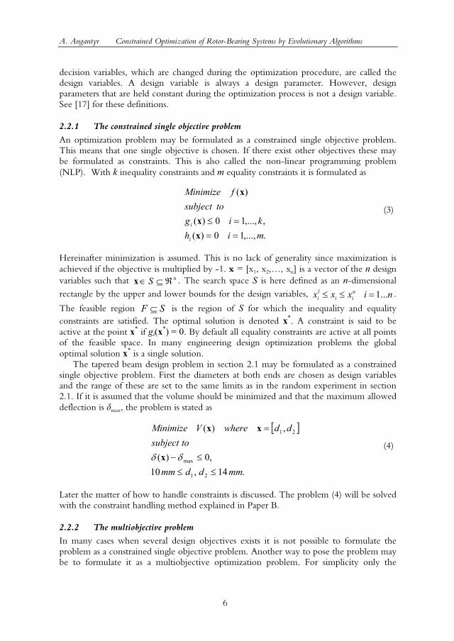
6
decision variables, which are changed during the optimization procedure, are called the design variables. A design variable is always a design parameter. However, design parameters that are held constant during the optimization process is not a design variable. See [17] for these definitions.
2.2.1 The constrained single objective problem
An optimization problem may be formulated as a constrained single objective problem. This means that one single objective is chosen. If there exist other objectives these may be formulated as constraints. This is also called the non-linear programming problem (NLP). With k inequality constraints and m equality constraints it is formulated as
.,...,10)(,,...,10)(
)(
mihkig
tosubjectfMinimize
i
i
===≤
xx
x
(3)
Hereinafter minimization is assumed. This is no lack of generality since maximization is achieved if the objective is multiplied by -1. x = [x1, x2,, xn] is a vector of the n design variables such that nS ℜ⊆∈x . The search space S is here defined as an n-dimensional rectangle by the upper and lower bounds for the design variables, 1...l u
i i ix x x i n≤ ≤ = .
The feasible region SF ⊆ is the region of S for which the inequality and equality constraints are satisfied. The optimal solution is denoted x*. A constraint is said to be active at the point x* if gi(x*) = 0. By default all equality constraints are active at all points of the feasible space. In many engineering design optimization problems the global optimal solution x* is a single solution. The tapered beam design problem in section 2.1 may be formulated as a constrained single objective problem. First the diameters at both ends are chosen as design variables and the range of these are set to the same limits as in the random experiment in section 2.1. If it is assumed that the volume should be minimized and that the maximum allowed deflection is δmax, the problem is stated as
[ ]
.14,10,0)(
,)(
21
max
21
mmddmm
tosubjectddwhereVMinimize
≤≤≤−
=
δδ x
xx
(4)
Later the matter of how to handle constraints is discussed. The problem (4) will be solved with the constraint handling method explained in Paper B.
2.2.2 The multiobjective problem
In many cases when several design objectives exists it is not possible to formulate the problem as a constrained single objective problem. Another way to pose the problem may be to formulate it as a multiobjective optimization problem. For simplicity only the
A. Angantyr Constrained Optimization of Rotor-Bearing Systems by Evolutionary Algorithms
7
unconstrained multiobjective problem is considered here. For k objectives it may be formulated as
[ ]
.
)(..,),(),()( 21
Stosubject
fffMinimize k
∈
=
x
xxxxF (5)
S is the search space usually defined as an n-dimensional rectangle as in the constrained single objective problem formulation. The problem is now to search for solutions which minimize all the objectives fi(x). If there exists a solution which simultaneously minimizes all the objectives this is called the utopian solution. In the general case when some objectives are in conflict with each other it is however not possible to find the utopian solution. The solution that is searched for should in this case be a member of the non-dominated set of solutions. According to [18] a solution x is said to dominate a solution y if the following holds:
)()(:..,,2,1)()(:..,,2,1 yxyx jjii ffkjandffki <∈∃≤∈∀
(6)
What equation (6) says is that a solution dominates another solution if it is better in at least one objective and not worse in the other objectives. With the terminology used here and the definition according to Deb [19] the non-dominated set of solutions is defined as: Among a set of solutions S, the non-dominated set of solutions P are those that are not dominated by any member of the set S. This set is also called the Pareto optimal set of solutions. A short discussion of possible techniques to solve (5) will be done in section 3.4. Lets just mention that there exist methods that try to find the whole Pareto optimal set in one single optimization run. A multiobjective GA which is one such method will be discussed later. Paper A presents a rotor-bearing optimization problem of type (5). A multiobjective formulation of the tapered beam design problem may be stated as
[ ] [ ]
.14,10
,)(),()(
21
21
mmddmmtosubject
ddwhereVMinimize
≤≤
== xxxxF δ (7)
The Pareto optimal set of solutions for problem (7) is shown in the objective space as the red line in Figure 2. In section 3.4 an example of how this set may be evolved with a GA is presented.
2.3 Practical aspects of engineering design optimization In order to achieve a successful final design, a good conceptual design is of course required. Since most products actually are based on redesign and modifications of existing concepts, optimization in the late design stage is be motivated. Optimized products are especially important for high performance, large and expensive or high volume products. An important aspect is that there are always some overhead costs related to perform optimizations in the design process. Before one starts with any optimization one should therefore always pose the question: Does the potential gain in product performance, cost, etc
A. Angantyr Constrained Optimization of Rotor-Bearing Systems by Evolutionary Algorithms
8
motivate the use of optimization methods in this particular case? If the answer is yes or probably one may proceed and start formulating and then solving the problem. Worth to note is that the use of optimization techniques is not only restricted to the late design stage. The only requirement is that a mathematical model exists of the product/system to optimize. The mathematical models used in this thesis are explained in section 4. Most books on engineering design optimization go directly into the details of the algorithms. An engineer working with design optimization is usually more interested to solve the problem than how to solve it. Therefore stable and robust algorithms that work for a large number of problems are motivated. Before even thinking about how to solve it, the engineer is faced the important challenge to formulate the problem. These are a few aspects that affect the problem formulation.
• Which design variables should be chosen? • What is the objective and what are the constraints? • Often a mix of design variables exists (continuous, discrete, categorical). • Almost always several objectives exist.
In practice, the choice of design variables is often given by the fact that all design parameters are not possible to change. However, one should not just choose all the design parameters that may be subject to changes as design variables. The chosen design variables should have effect on the response of the system. Design parameters which only have minor effect on the system response could probably be excluded as design variables. In practical problem it is often difficult to decide what is objective and what are constraints? If it several objectives exist, the formulation might be a multiobjective optimization problem (5). If some of the objectives may be formulated as constraints instead, this is preferable since the problem will in general become easier to solve. An optimization problem with only discrete design variable is a combinatorial problem with a finite set of solutions. If some design variable is of continuous type, the search space is a set of infinitely many solutions. Many real-world design problems involves mixed types of design variables. In the next section a few methods that may be used to tackle these kinds of problem is presented. Before the formulation of the problem is done it is always good to get as much information as possible about the system. The strategy used by the author in this thesis is summarized as follows.
1. Chose design variables
2. Perform a numerical experiment
3. Formulate the optimization problem
4. Optimize
5. Post-optimal analysis
The purpose of the initial numerical experiment is to get an overview of what possibly might be achieved in the later optimization. It may for example also show that some design variables are not relevant and therefore can be excluded. Design of experiments (DOE) is a large field, see Montgomery [20]. A simple Monte Carlo method has been used by the author in Paper A, Paper C and Paper D. Hence, solutions are randomly generated in the search space. Even though there exist more advanced methods this
A. Angantyr Constrained Optimization of Rotor-Bearing Systems by Evolutionary Algorithms
9
method should not be neglected since it may serve its purpose for large and complex problems with many constraints and possibly several objectives. When an optimal solution is found it is of interest to know how robust the solution is. This is investigated in the post-optimal analysis phase. A robust solution is a solution that gives only small effects in response for perturbations in the design parameters. In the case of a multiobjective problem, robustness may be the base for the final decision of which solution to choose from the Pareto optimal set.
2.4 Some optimization methods The purpose for this section is to present a short review of some of the most important search and optimization methods used in engineering design optimization. It should be clear that a comprehensive survey of all existing optimization methods is far beyond the scope for this section. The interested reader is therefore encouraged to read the introductory book by Onwubiko [17] or the more comprehensive book by Rao [21]. Traditionally there has been a large focus on methods that use gradient information in the search process, i.e. gradient based methods. Gradient based methods are efficient for convex objective functions and if the number of design variables is not too high. A drawback that frequently appears for real-world problems is that the result often is dependent on an initial start guess. Engineering design problems often involves non-convex objective functions or even disjointed search spaces. The focus in this section is therefore directed towards methods that are better suited for this kind of problems. Still one should not reject the use of gradient based methods on problem with continuous design variables and convex objective functions. A subject closely connected to engineering design optimization is DOE, Montgomery [20]. Before an optimization is conducted it is good to have some knowledge of the behavior of the system. This is where DOE may come in. DOE may also be used in the post optimal analysis phase. Methods related to DOE and robustness of the system is response surface methods (RSM) [22]. In these methods an initial experiment is set up and conducted. The objective function is then approximated by usually a second order polynomial response surface. The experiment may be repeated so that a more accurate response surface is been obtained. These methods are suitable if the number of design variables is low. Another more advanced approximation technique for problems with costly and noisy objective functions is to train neural networks [23] to simulate the behavior of the system. There are different ways to classify search and optimization methods. In [24] Hajela reviews some non-gradient based search and optimization methods. He also distinguishes between zero-order methods for local search and methods for global search. Some of these methods are listed in Table 2.

A. Angantyr Constrained Optimization of Rotor-Bearing Systems by Evolutionary Algorithms
10
Table 2. Some non-gradient based search and optimization methods classified according to Hajela [24].
Zero-order methods for local search
Methods for global search
Hookes-Jeeves [17] Sequential quadratic programming [17] Nelder-Mead simplex [17] -
Deterministic
Complex [25] - Random walk [24] Simulated Annealing (SA) [26] Stochastic - Evolutionary Algorithms (EAs)
Zero-order methods use only the objective function value and no gradient information. The progress in the optimization process for the deterministic methods is based on predefined rules. In the stochastic methods, a certain amount of randomization is used in the search process. These methods are computationally expensive in terms of the many required objective function evaluations but they are also robust. During the past decade stochastic global search methods has become more and more important as tools in engineering design optimization problems. In [24] Hajela says that These methods have emerged as potent tools for locating optimal designs in problems that are generally regarded as difficult. Simulated Annealing (SA) is based on ideas from statistical mechanics and thermodynamics. If a metal piece is slowly cooled from an initially high temperature it takes the state which minimizes the potential energy. This is completely analog to the working principles of SA. Evolutionary Algorithms (EAs) are based on principles found in natural evolution. The background of these methods is described in some more detail in the next section. It is worth to note that there exists no best method for all cases. Even in a single case, this method may not exist. Probably the best choice is a hybrid method that starts with a global search method to locate the interesting region of the search space followed by a fast local search method.
2.5 Evolutionary algorithms EAs is a class of global search algorithms inspired by natural evolution. Several different types of EAs exist. Genetic Algorithms (GAs), Evolution Strategies (ES), Evolutionary Programming (EP) and Genetic Programming (GP) are some of the most known. In this work, real coded Genetic Algorithms (explained in section 3.1) have been used extensively. Real coded GAs is in many aspects similar to ES. Therefore a short historical recap of GAs and ES is given in the next section.
2.5.1 Historical perspective
During the early 1970s Holland [27] and his students presented the first work in the field of GAs. At almost the same time, Rechenberg [28] and colleagues worked with ES. ES and GAs are quite similar but there are important differences. ES work with real design variables while GAs work with a binary coding of the design variables, see section 3.1. Furthermore, the search operator in ES is a mutation operator. In a GA this is a secondary operator since the fundamental search operator here is a crossover operation. During the 1980s real coded GAs began to pop up. At this point it becomes difficult to distinguish
A. Angantyr Constrained Optimization of Rotor-Bearing Systems by Evolutionary Algorithms
11
between ES and GAs. In section 3 the background and principles of GAs are given in some more detail.
2.5.2 Why and when to use EAs?
The natural evolution is a slow process. Hence, EAs are also quite slow compared to many other optimization algorithms, i.e. on continuous and convex functions. But it is also important that they are robust algorithms. EAs are a good choice for multimodal and noisy objective functions. It is also shown that EAs are suitable on many combinatorial problems with large search spaces. If the number of design variables is high, EAs may be one possible choice. EAs may also be the choice if there is a mix of different types of design variables. EAs should not be used if local search is of importance, nor should they be used when the objective function evaluations are computationally expensive.
A. Angantyr Constrained Optimization of Rotor-Bearing Systems by Evolutionary Algorithms
12
3 Genetic algorithms GAs has been used extensively in this work. The purpose of this section is to introduce the reader into the basics of GAs. Since GAs is a huge field itself, it should be clear that what will be presented here are only selected parts which the author finds most necessary. GAs is one type of EAs which originates from the work by Holland [27] in the early 1970s. Two other good text books on the subject are [29] by Goldberg and [30] by Davis. Traditionally GAs works with binary coding of the problem. This will be explained in the next section. Nowadays there exist GAs that works on data structures which is more similar to the specific problem, for example real numbers. The book by Gen and Cheng [31] gives some introduction to this subject. Another more recent, comprehensive book which may serve as a work of reference for the fundamentals of GAs and especially multiobjective GAs is [19] by Deb.
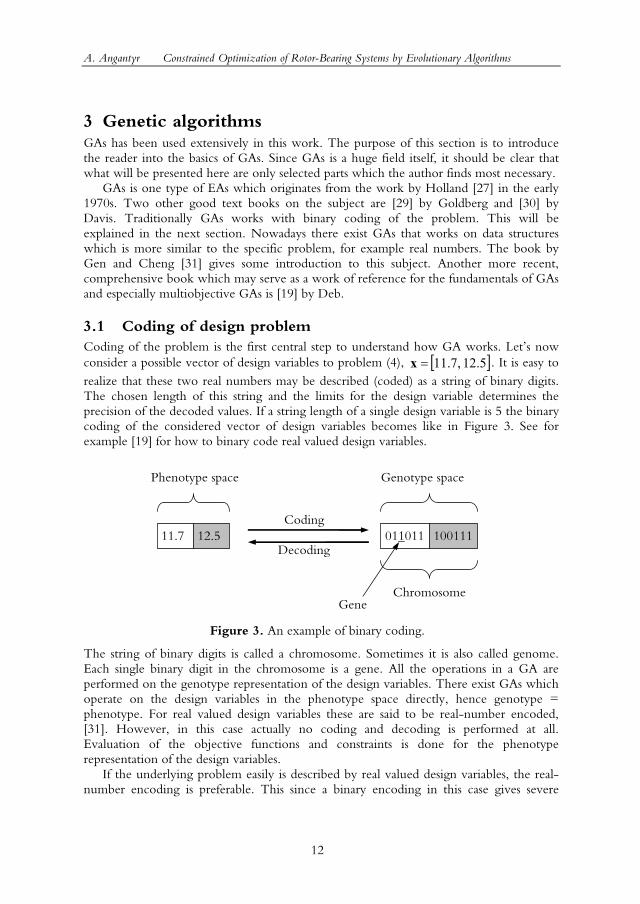
3.1 Coding of design problem Coding of the problem is the first central step to understand how GA works. Lets now consider a possible vector of design variables to problem (4), [ ]5.12,7.11=x . It is easy to realize that these two real numbers may be described (coded) as a string of binary digits. The chosen length of this string and the limits for the design variable determines the precision of the decoded values. If a string length of a single design variable is 5 the binary coding of the considered vector of design variables becomes like in Figure 3. See for example [19] for how to binary code real valued design variables.
Figure 3. An example of binary coding.
The string of binary digits is called a chromosome. Sometimes it is also called genome. Each single binary digit in the chromosome is a gene. All the operations in a GA are performed on the genotype representation of the design variables. There exist GAs which operate on the design variables in the phenotype space directly, hence genotype = phenotype. For real valued design variables these are said to be real-number encoded, [31]. However, in this case actually no coding and decoding is performed at all. Evaluation of the objective functions and constraints is done for the phenotype representation of the design variables. If the underlying problem easily is described by real valued design variables, the real-number encoding is preferable. This since a binary encoding in this case gives severe
11.7 12.5 011011 100111 Coding
Decoding
Phenotype space Genotype space
Chromosome Gene
A. Angantyr Constrained Optimization of Rotor-Bearing Systems by Evolutionary Algorithms
13
drawbacks with Hamming cliffs, [31]. In most cases it is preferable to choose a coding that gives a genotype representation which is as similar as possible to the phenotype representation.
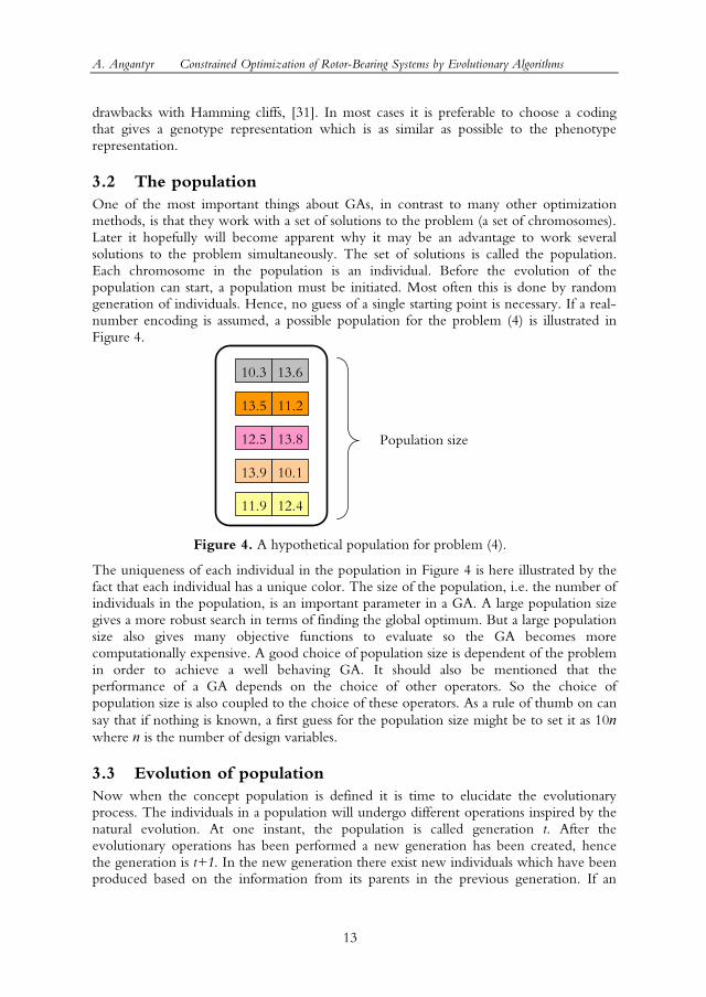
3.2 The population One of the most important things about GAs, in contrast to many other optimization methods, is that they work with a set of solutions to the problem (a set of chromosomes). Later it hopefully will become apparent why it may be an advantage to work several solutions to the problem simultaneously. The set of solutions is called the population. Each chromosome in the population is an individual. Before the evolution of the population can start, a population must be initiated. Most often this is done by random generation of individuals. Hence, no guess of a single starting point is necessary. If a real-number encoding is assumed, a possible population for the problem (4) is illustrated in Figure 4.
Figure 4. A hypothetical population for problem (4).
The uniqueness of each individual in the population in Figure 4 is here illustrated by the fact that each individual has a unique color. The size of the population, i.e. the number of individuals in the population, is an important parameter in a GA. A large population size gives a more robust search in terms of finding the global optimum. But a large population size also gives many objective functions to evaluate so the GA becomes more computationally expensive. A good choice of population size is dependent of the problem in order to achieve a well behaving GA. It should also be mentioned that the performance of a GA depends on the choice of other operators. So the choice of population size is also coupled to the choice of these operators. As a rule of thumb on can say that if nothing is known, a first guess for the population size might be to set it as 10n where n is the number of design variables.
3.3 Evolution of population Now when the concept population is defined it is time to elucidate the evolutionary process. The individuals in a population will undergo different operations inspired by the natural evolution. At one instant, the population is called generation t. After the evolutionary operations has been performed a new generation has been created, hence the generation is t+1. In the new generation there exist new individuals which have been produced based on the information from its parents in the previous generation. If an
10.3 13.6
Population size
13.5 11.2
12.5 13.8
13.9 10.1
11.9 12.4
A. Angantyr Constrained Optimization of Rotor-Bearing Systems by Evolutionary Algorithms
14
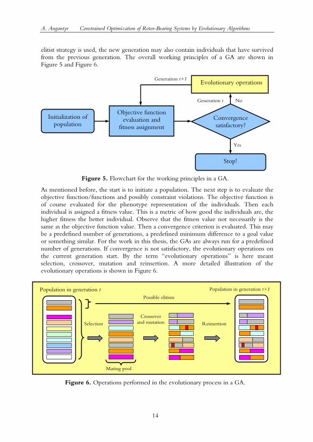
elitist strategy is used, the new generation may also contain individuals that have survived from the previous generation. The overall working principles of a GA are shown in Figure 5 and Figure 6.
Figure 5. Flowchart for the working principles in a GA.
As mentioned before, the start is to initiate a population. The next step is to evaluate the objective function/functions and possibly constraint violations. The objective function is of course evaluated for the phenotype representation of the individuals. Then each individual is assigned a fitness value. This is a metric of how good the individuals are, the higher fitness the better individual. Observe that the fitness value not necessarily is the same as the objective function value. Then a convergence criterion is evaluated. This may be a predefined number of generations, a predefined minimum difference to a goal value or something similar. For the work in this thesis, the GAs are always run for a predefined number of generations. If convergence is not satisfactory, the evolutionary operations on the current generation start. By the term evolutionary operations is here meant selection, crossover, mutation and reinsertion. A more detailed illustration of the evolutionary operations is shown in Figure 6.
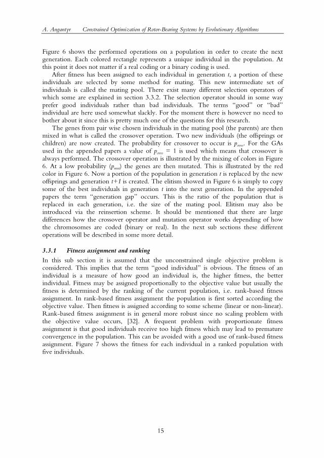
Figure 6. Operations performed in the evolutionary process in a GA.
Initialization of population
Objective function evaluation and
fitness assignment
Convergence satisfactory?
Evolutionary operations
Stop!
Generation t+1
Generation t No
Yes
Population in generation t Population in generation t+1
Possible elitism
Selection
Crossover and mutation Reinsertion
Mating pool
A. Angantyr Constrained Optimization of Rotor-Bearing Systems by Evolutionary Algorithms
15
Figure 6 shows the performed operations on a population in order to create the next generation. Each colored rectangle represents a unique individual in the population. At this point it does not matter if a real coding or a binary coding is used. After fitness has been assigned to each individual in generation t, a portion of these individuals are selected by some method for mating. This new intermediate set of individuals is called the mating pool. There exist many different selection operators of which some are explained in section 3.3.2. The selection operator should in some way prefer good individuals rather than bad individuals. The terms good or bad individual are here used somewhat slackly. For the moment there is however no need to bother about it since this is pretty much one of the questions for this research. The genes from pair wise chosen individuals in the mating pool (the parents) are then mixed in what is called the crossover operation. Two new individuals (the offsprings or children) are now created. The probability for crossover to occur is pcross. For the GAs used in the appended papers a value of pcross = 1 is used which means that crossover is always performed. The crossover operation is illustrated by the mixing of colors in Figure 6. At a low probability (pmut) the genes are then mutated. This is illustrated by the red color in Figure 6. Now a portion of the population in generation t is replaced by the new offsprings and generation t+1 is created. The elitism showed in Figure 6 is simply to copy some of the best individuals in generation t into the next generation. In the appended papers the term generation gap occurs. This is the ratio of the population that is replaced in each generation, i.e. the size of the mating pool. Elitism may also be introduced via the reinsertion scheme. It should be mentioned that there are large differences how the crossover operator and mutation operator works depending of how the chromosomes are coded (binary or real). In the next sub sections these different operations will be described in some more detail.
3.3.1 Fitness assignment and ranking
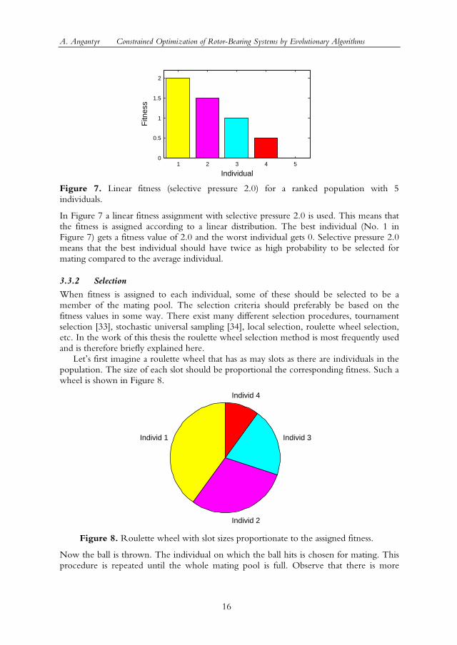
In this sub section it is assumed that the unconstrained single objective problem is considered. This implies that the term good individual is obvious. The fitness of an individual is a measure of how good an individual is, the higher fitness, the better individual. Fitness may be assigned proportionally to the objective value but usually the fitness is determined by the ranking of the current population, i.e. rank-based fitness assignment. In rank-based fitness assignment the population is first sorted according the objective value. Then fitness is assigned according to some scheme (linear or non-linear). Rank-based fitness assignment is in general more robust since no scaling problem with the objective value occurs, [32]. A frequent problem with proportionate fitness assignment is that good individuals receive too high fitness which may lead to premature convergence in the population. This can be avoided with a good use of rank-based fitness assignment. Figure 7 shows the fitness for each individual in a ranked population with five individuals.
A. Angantyr Constrained Optimization of Rotor-Bearing Systems by Evolutionary Algorithms
16
1 2 3 4 5
0
0.5
1
1.5
2
Fitn
ess
Individual
Figure 7. Linear fitness (selective pressure 2.0) for a ranked population with 5 individuals.
In Figure 7 a linear fitness assignment with selective pressure 2.0 is used. This means that the fitness is assigned according to a linear distribution. The best individual (No. 1 in Figure 7) gets a fitness value of 2.0 and the worst individual gets 0. Selective pressure 2.0 means that the best individual should have twice as high probability to be selected for mating compared to the average individual.
3.3.2 Selection
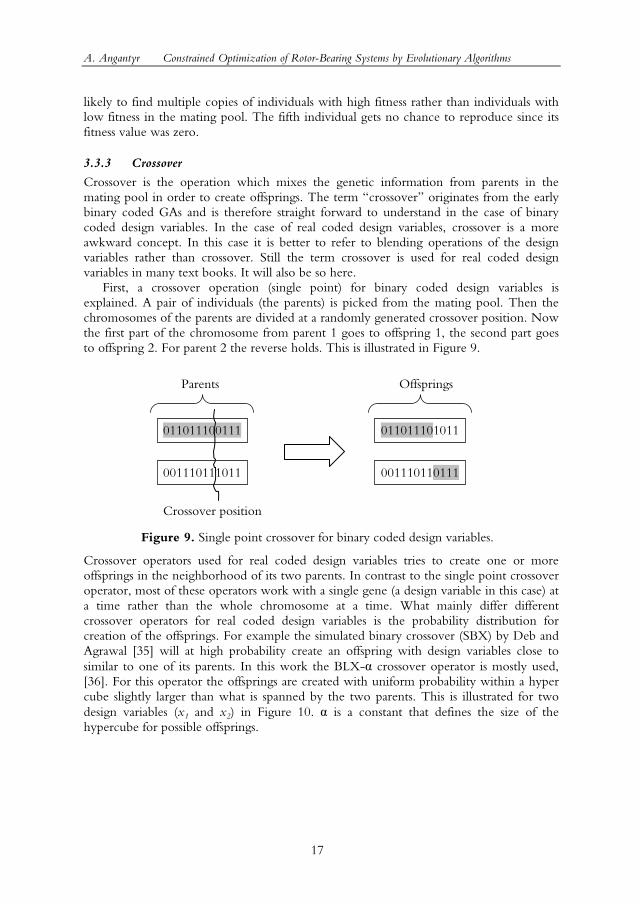
When fitness is assigned to each individual, some of these should be selected to be a member of the mating pool. The selection criteria should preferably be based on the fitness values in some way. There exist many different selection procedures, tournament selection [33], stochastic universal sampling [34], local selection, roulette wheel selection, etc. In the work of this thesis the roulette wheel selection method is most frequently used and is therefore briefly explained here. Lets first imagine a roulette wheel that has as may slots as there are individuals in the population. The size of each slot should be proportional the corresponding fitness. Such a wheel is shown in Figure 8.
Individ 1
Individ 2
Individ 3
Individ 4
Figure 8. Roulette wheel with slot sizes proportionate to the assigned fitness.
Now the ball is thrown. The individual on which the ball hits is chosen for mating. This procedure is repeated until the whole mating pool is full. Observe that there is more
A. Angantyr Constrained Optimization of Rotor-Bearing Systems by Evolutionary Algorithms
17
likely to find multiple copies of individuals with high fitness rather than individuals with low fitness in the mating pool. The fifth individual gets no chance to reproduce since its fitness value was zero.
3.3.3 Crossover
Crossover is the operation which mixes the genetic information from parents in the mating pool in order to create offsprings. The term crossover originates from the early binary coded GAs and is therefore straight forward to understand in the case of binary coded design variables. In the case of real coded design variables, crossover is a more awkward concept. In this case it is better to refer to blending operations of the design variables rather than crossover. Still the term crossover is used for real coded design variables in many text books. It will also be so here. First, a crossover operation (single point) for binary coded design variables is explained. A pair of individuals (the parents) is picked from the mating pool. Then the chromosomes of the parents are divided at a randomly generated crossover position. Now the first part of the chromosome from parent 1 goes to offspring 1, the second part goes to offspring 2. For parent 2 the reverse holds. This is illustrated in Figure 9.
Figure 9. Single point crossover for binary coded design variables.
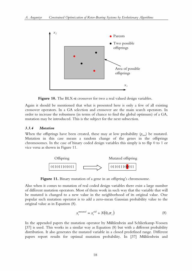
Crossover operators used for real coded design variables tries to create one or more offsprings in the neighborhood of its two parents. In contrast to the single point crossover operator, most of these operators work with a single gene (a design variable in this case) at a time rather than the whole chromosome at a time. What mainly differ different crossover operators for real coded design variables is the probability distribution for creation of the offsprings. For example the simulated binary crossover (SBX) by Deb and Agrawal [35] will at high probability create an offspring with design variables close to similar to one of its parents. In this work the BLX-α crossover operator is mostly used, [36]. For this operator the offsprings are created with uniform probability within a hyper cube slightly larger than what is spanned by the two parents. This is illustrated for two design variables (x1 and x2) in Figure 10. α is a constant that defines the size of the hypercube for possible offsprings.
011011100111
Crossover position
Parents Offsprings
001110111011
011011101011
001110110111
A. Angantyr Constrained Optimization of Rotor-Bearing Systems by Evolutionary Algorithms
18
Figure 10. The BLX-α crossover for two a real valued design variables.
Again it should be mentioned that what is presented here is only a few of all existing crossover operators. In a GA selection and crossover are the main search operators. In order to increase the robustness (in terms of chance to find the global optimum) of a GA, mutation may be introduced. This is the subject for the next subsection.
3.3.4 Mutation
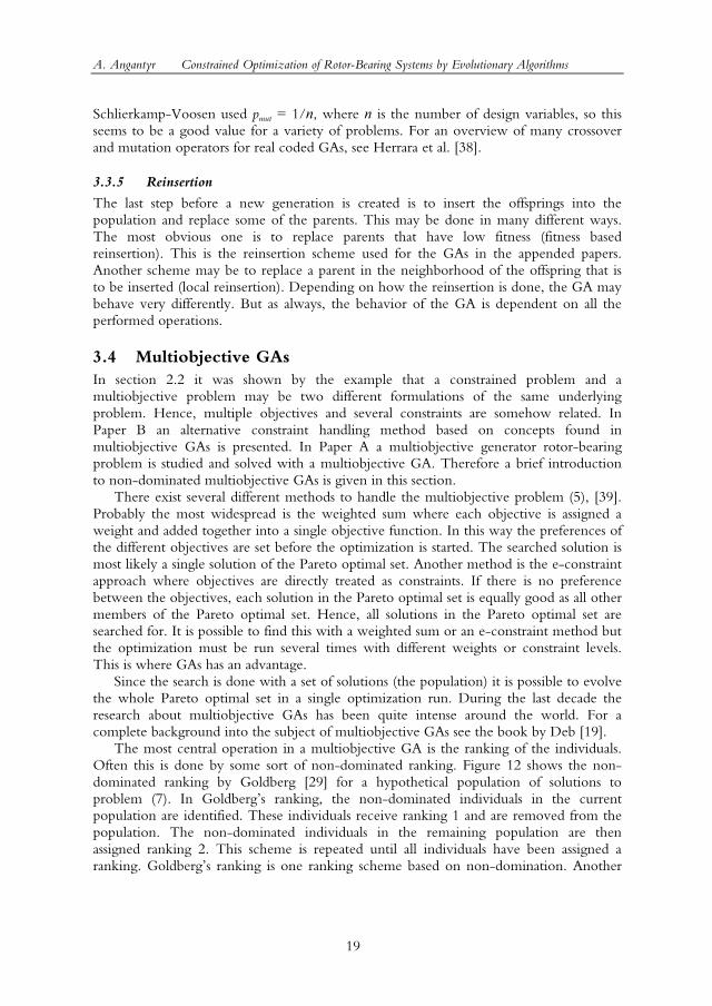
When the offsprings have been created, these may at low probability (pmut) be mutated. Mutation in this case means a random change of the genes in the offsprings chromosomes. In the case of binary coded design variables this simply is to flip 0 to 1 or vice versa as shown in Figure 11.
Figure 11. Binary mutation of a gene in an offsprings chromosome.
Also when it comes to mutation of real coded design variables there exist a large number of different mutation operators. Most of them work in such way that the variable that will be mutated is changed to a new value in the neighborhood of its original value. One popular such mutation operator is to add a zero-mean Gaussian probability value to the original value as in Equation (8).
( )ioldi
mutatedi Nxx σ,0+= (8)
In the appended papers the mutation operator by Mühlenbein and Schlierkamp-Voosen [37] is used. This works in a similar way as Equation (8) but with a different probability distribution. It also generates the mutated variable in a closed predefined range. Different papers report results for optimal mutation probability. In [37] Mühlenbein and
Offspring Mutated offspring
011011101011 011011100011
x2
x1
Parents
Area of possible offsprings
Two possible offsprings
A. Angantyr Constrained Optimization of Rotor-Bearing Systems by Evolutionary Algorithms
19
Schlierkamp-Voosen used pmut = 1/n, where n is the number of design variables, so this seems to be a good value for a variety of problems. For an overview of many crossover and mutation operators for real coded GAs, see Herrara et al. [38].
3.3.5 Reinsertion
The last step before a new generation is created is to insert the offsprings into the population and replace some of the parents. This may be done in many different ways. The most obvious one is to replace parents that have low fitness (fitness based reinsertion). This is the reinsertion scheme used for the GAs in the appended papers. Another scheme may be to replace a parent in the neighborhood of the offspring that is to be inserted (local reinsertion). Depending on how the reinsertion is done, the GA may behave very differently. But as always, the behavior of the GA is dependent on all the performed operations.
3.4 Multiobjective GAs In section 2.2 it was shown by the example that a constrained problem and a multiobjective problem may be two different formulations of the same underlying problem. Hence, multiple objectives and several constraints are somehow related. In Paper B an alternative constraint handling method based on concepts found in multiobjective GAs is presented. In Paper A a multiobjective generator rotor-bearing problem is studied and solved with a multiobjective GA. Therefore a brief introduction to non-dominated multiobjective GAs is given in this section. There exist several different methods to handle the multiobjective problem (5), [39]. Probably the most widespread is the weighted sum where each objective is assigned a weight and added together into a single objective function. In this way the preferences of the different objectives are set before the optimization is started. The searched solution is most likely a single solution of the Pareto optimal set. Another method is the e-constraint approach where objectives are directly treated as constraints. If there is no preference between the objectives, each solution in the Pareto optimal set is equally good as all other members of the Pareto optimal set. Hence, all solutions in the Pareto optimal set are searched for. It is possible to find this with a weighted sum or an e-constraint method but the optimization must be run several times with different weights or constraint levels. This is where GAs has an advantage. Since the search is done with a set of solutions (the population) it is possible to evolve the whole Pareto optimal set in a single optimization run. During the last decade the research about multiobjective GAs has been quite intense around the world. For a complete background into the subject of multiobjective GAs see the book by Deb [19]. The most central operation in a multiobjective GA is the ranking of the individuals. Often this is done by some sort of non-dominated ranking. Figure 12 shows the non-dominated ranking by Goldberg [29] for a hypothetical population of solutions to problem (7). In Goldbergs ranking, the non-dominated individuals in the current population are identified. These individuals receive ranking 1 and are removed from the population. The non-dominated individuals in the remaining population are then assigned ranking 2. This scheme is repeated until all individuals have been assigned a ranking. Goldbergs ranking is one ranking scheme based on non-domination. Another
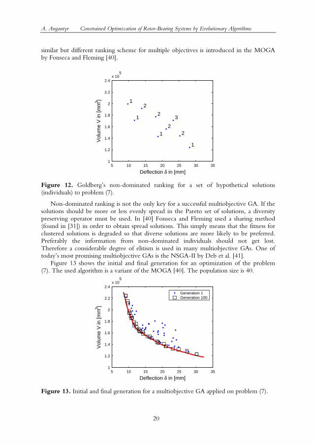
A. Angantyr Constrained Optimization of Rotor-Bearing Systems by Evolutionary Algorithms
20
similar but different ranking scheme for multiple objectives is introduced in the MOGA by Fonseca and Fleming [40].
5 10 15 20 25 30 351
1.2
1.4
1.6
1.8
2
2.2
2.4x 10
5
1
1
1
12
2
22
3
Deflection δ in [mm]
Vol
ume
V in
[mm
3 ]
Figure 12. Goldbergs non-dominated ranking for a set of hypothetical solutions (individuals) to problem (7).
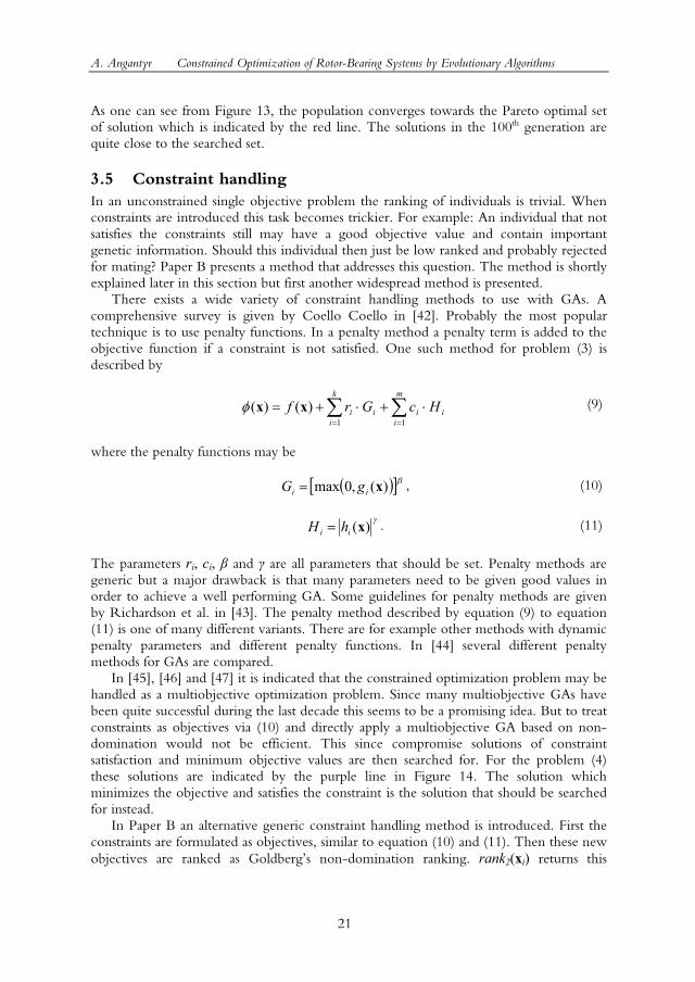
Non-dominated ranking is not the only key for a successful multiobjective GA. If the solutions should be more or less evenly spread in the Pareto set of solutions, a diversity preserving operator must be used. In [40] Fonseca and Fleming used a sharing method (found in [31]) in order to obtain spread solutions. This simply means that the fitness for clustered solutions is degraded so that diverse solutions are more likely to be preferred. Preferably the information from non-dominated individuals should not get lost. Therefore a considerable degree of elitism is used in many multiobjective GAs. One of todays most promising multiobjective GAs is the NSGA-II by Deb et al. [41]. Figure 13 shows the initial and final generation for an optimization of the problem (7). The used algorithm is a variant of the MOGA [40]. The population size is 40.
5 10 15 20 25 30 351
1.2
1.4
1.6
1.8
2
2.2
2.4x 10
5
Deflection δ in [mm]
Vol
ume
V in
[mm
3 ]
Generation 1Generation 100
Figure 13. Initial and final generation for a multiobjective GA applied on problem (7).
A. Angantyr Constrained Optimization of Rotor-Bearing Systems by Evolutionary Algorithms
21
As one can see from Figure 13, the population converges towards the Pareto optimal set of solution which is indicated by the red line. The solutions in the 100th generation are quite close to the searched set.
3.5 Constraint handling In an unconstrained single objective problem the ranking of individuals is trivial. When constraints are introduced this task becomes trickier. For example: An individual that not satisfies the constraints still may have a good objective value and contain important genetic information. Should this individual then just be low ranked and probably rejected for mating? Paper B presents a method that addresses this question. The method is shortly explained later in this section but first another widespread method is presented. There exists a wide variety of constraint handling methods to use with GAs. A comprehensive survey is given by Coello Coello in [42]. Probably the most popular technique is to use penalty functions. In a penalty method a penalty term is added to the objective function if a constraint is not satisfied. One such method for problem (3) is described by
∑∑==
⋅+⋅+=m
iii
k
iii HcGrf
11)()( xxφ (9)
where the penalty functions may be
( )[ ]β)(,0max xii gG = , (10)
γ)(xii hH = . (11)
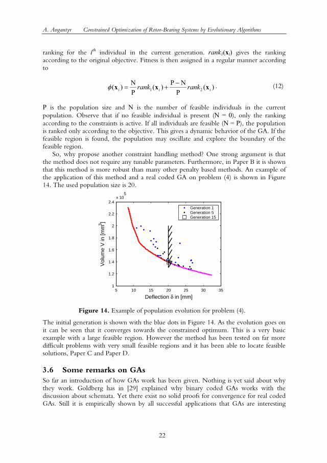
The parameters ri, ci, β and γ are all parameters that should be set. Penalty methods are generic but a major drawback is that many parameters need to be given good values in order to achieve a well performing GA. Some guidelines for penalty methods are given by Richardson et al. in [43]. The penalty method described by equation (9) to equation (11) is one of many different variants. There are for example other methods with dynamic penalty parameters and different penalty functions. In [44] several different penalty methods for GAs are compared. In [45], [46] and [47] it is indicated that the constrained optimization problem may be handled as a multiobjective optimization problem. Since many multiobjective GAs have been quite successful during the last decade this seems to be a promising idea. But to treat constraints as objectives via (10) and directly apply a multiobjective GA based on non-domination would not be efficient. This since compromise solutions of constraint satisfaction and minimum objective values are then searched for. For the problem (4) these solutions are indicated by the purple line in Figure 14. The solution which minimizes the objective and satisfies the constraint is the solution that should be searched for instead. In Paper B an alternative generic constraint handling method is introduced. First the constraints are formulated as objectives, similar to equation (10) and (11). Then these new objectives are ranked as Goldbergs non-domination ranking. rank2(xi) returns this
A. Angantyr Constrained Optimization of Rotor-Bearing Systems by Evolutionary Algorithms
22
ranking for the ith individual in the current generation. rank1(xi) gives the ranking according to the original objective. Fitness is then assigned in a regular manner according to
)(P
NP)(PN)( 21 iii rankrank xxx −
+=φ . (12)
P is the population size and N is the number of feasible individuals in the current population. Observe that if no feasible individual is present (N = 0), only the ranking according to the constraints is active. If all individuals are feasible (N = P), the population is ranked only according to the objective. This gives a dynamic behavior of the GA. If the feasible region is found, the population may oscillate and explore the boundary of the feasible region. So, why propose another constraint handling method? One strong argument is that the method does not require any tunable parameters. Furthermore, in Paper B it is shown that this method is more robust than many other penalty based methods. An example of the application of this method and a real coded GA on problem (4) is shown in Figure 14. The used population size is 20.
5 10 15 20 25 30 351
1.2
1.4
1.6
1.8
2
2.2
2.4x 10
5
Deflection δ in [mm]
Vol
ume
V in
[mm
3 ]
Generation 1Generation 5Generation 15
Figure 14. Example of population evolution for problem (4).
The initial generation is shown with the blue dots in Figure 14. As the evolution goes on it can be seen that it converges towards the constrained optimum. This is a very basic example with a large feasible region. However the method has been tested on far more difficult problems with very small feasible regions and it has been able to locate feasible solutions, Paper C and Paper D.
3.6 Some remarks on GAs So far an introduction of how GAs work has been given. Nothing is yet said about why they work. Goldberg has in [29] explained why binary coded GAs works with the discussion about schemata. Yet there exist no solid proofs for convergence for real coded GAs. Still it is empirically shown by all successful applications that GAs are interesting
A. Angantyr Constrained Optimization of Rotor-Bearing Systems by Evolutionary Algorithms
23
methods for difficult real-world problems. Much of the current research about GAs (for example Paper B) is experimental in nature. As mentioned earlier, one of the most important features of a GA is that the search is done with a set of solutions. This also gives some interesting possibilities. As show in section 3.4 it is possible to evolve an approximation to the Pareto optimal set of solutions in a multiobjective problem. In a single objective multi modal problem this makes it possible to locate several local optima if niching is introduced. The knowledge of several local optima is important if the robustness of the solutions is considered. It may be better to choose a locally optimal solution than the global optimal solution if the former is less sensitive to changes in some parameters. Another interesting thing about GAs and robustness of solutions is that it is possible to evolve only robust solutions and reject solutions from narrow optimum. This can be done by disturbing the design variables or other parameters during the evolutionary process [18]. The population based model also implies that GAs are inherently parallel. This since the objective functions that are to be evaluated for one single generation may be evaluated in parallel. The GA used in Paper D is paralellized and run on a Linux cluster of standard PCs. Four nodes are used for the calculations.
A. Angantyr Constrained Optimization of Rotor-Bearing Systems by Evolutionary Algorithms
24
4 Rotor-bearing system analysis and design The purpose of this section is to present some analysis models and methods that may be used to analyze rotating mechanical systems. Several special effects occur in the analysis of rotating system which seldom are found in other vibrating structures. The cause of these effects are therefore also briefly explained and discussed. At the end of this section the design process of large rotor-bearing systems is discussed and some practical design challenges are highlighted.
4.1 Rotordynamic analysis This thesis deals with the optimization of turbo generator and gas turbine rotor-bearing systems. The rotors in these systems are long compared to their diameters. This implies that they must be handled as continuous rotors. Since the geometry of these rotors is too complex in order to be handled by continuous models, approximate discretized models need to be used. This section deals only with the analysis of multi DOF (degree of freedom) models. For a deeper insight into the fundamentals of rotordynamics the reader is referred for example to the books by Genta [48] and Vance [49].
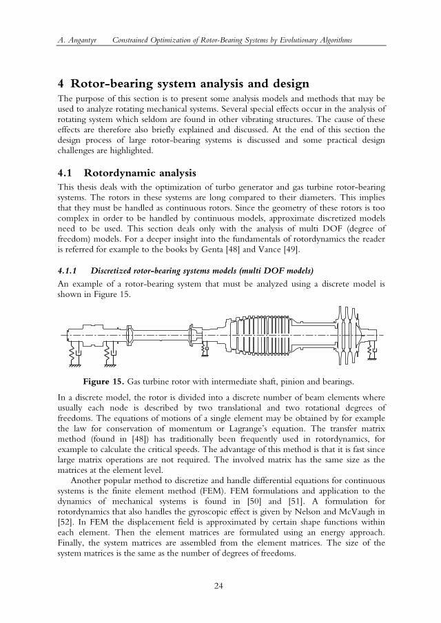
4.1.1 Discretized rotor-bearing systems models (multi DOF models)
An example of a rotor-bearing system that must be analyzed using a discrete model is shown in Figure 15.
Figure 15. Gas turbine rotor with intermediate shaft, pinion and bearings.
In a discrete model, the rotor is divided into a discrete number of beam elements where usually each node is described by two translational and two rotational degrees of freedoms. The equations of motions of a single element may be obtained by for example the law for conservation of momentum or Lagranges equation. The transfer matrix method (found in [48]) has traditionally been frequently used in rotordynamics, for example to calculate the critical speeds. The advantage of this method is that it is fast since large matrix operations are not required. The involved matrix has the same size as the matrices at the element level. Another popular method to discretize and handle differential equations for continuous systems is the finite element method (FEM). FEM formulations and application to the dynamics of mechanical systems is found in [50] and [51]. A formulation for rotordynamics that also handles the gyroscopic effect is given by Nelson and McVaugh in [52]. In FEM the displacement field is approximated by certain shape functions within each element. Then the element matrices are formulated using an energy approach. Finally, the system matrices are assembled from the element matrices. The size of the system matrices is the same as the number of degrees of freedoms.
A. Angantyr Constrained Optimization of Rotor-Bearing Systems by Evolutionary Algorithms
25
A third approach is the so called lumped parameter method. In this approach the continuous system is approximated by rigid bodies (the nodes) coupled by springs and dampers. In fact the transfer matrix method is a sort of lumped parameter method. In a lumped parameter method it is straight-forward to obtain the inertia matrix (mass matrix) but the stiffness matrix may be more difficult to find. A possibility is also to mix the lumped parameter approach and FEM. This is usually done in FEM and modal analysis in order to get the stiffness matrix and a diagonal inertia matrix. It should also be mentioned that the rotordynamical analysis in the appended papers is done with an in-house code based on the transfer matrix method. However, hereinafter in the thesis it is assumed that either a FEM approach or a lumped parameter method is used to obtain the system matrices. It might be worth to point out that the finite element method is only used to obtain the system matrices. The analysis of the equations of motions is something else. Assume now that q is a displacement vector in real coordinates that defines the position of each node with respect to a fixed reference frame. Then the assembled matrix equation of motion for a discretized rotor system is formulated as
( ) ( )tΩΩ=+Ω−+ sin2fKqqGCqM &&& . (13)
This equation is similar to the shaft element formulation used by Choi and Yang in [14]. The rotational frequency is Ω and the inertia matrix M. If a lumped approach is used, this matrix is diagonal and if a consistent approach is used it is a banded matrix. C is the damping matrix and G is the skew-symmetric gyroscopic matrix. The stiffness matrix for the shaft and the supports is K. The right hand side of equation (13) describes a harmonic unbalance force. It should be clear that the system may well be excited by other types of forces. If this is the case, the right hand side of equation (13) is different. For the models used in the appended papers no rotational (internal) damping is introduced. Therefore equation (13) is limited to the case where no rotational damping is present. In section 4.1.5 the effect of rotational damping is discussed. If the rotor is supported by journal bearings the system is not necessarily conservative. Hence, the stiffness matrix can be non-symmetric which implies that instability can occur. Furthermore, the only contribution to C comes from damping in the bearings and supports since this is the only damping assumed to be present. In Figure 15 the support is illustrated by dampers and springs but it should be mentioned that equation (13) is not restricted to these support models. More advanced modeling of the stator structure is possible. If a FEM approach is used, the question is how to discretize the stator or support structure, choose element formulation and how to assemble the matrices. If the number of degrees of freedoms becomes too high, one possibility may be to use a reduction technique Genta [48] to reduce the computational effort in the analysis of equation (13).
4.1.2 Analysis by the state space approach
There are different ways to analyze equation (13). Here the state space approach is used. It is often used in control of dynamical systems or numerical simulations. It is also an interesting method for analysis of problems of type (13) since the presence of damping and the gyroscopic matrix does not give rise to any trouble as for example in modal analysis. The state space approach is the most general approach since it gives the most
A. Angantyr Constrained Optimization of Rotor-Bearing Systems by Evolutionary Algorithms
26
general form of eigenvalue problem for mechanical systems. Furthermore, it does not require any particular shape of the matrices as long as the mass matrix is invertible. The mass matrix may for example be lumped or consistent. Lets first assume that the number of degrees of freedom is N. Hence, the size of the matrices in (13) is N×N. Now a new coordinate vector TTT qqx &,= is created. Then
equation (13) may be expanded to a set of 2N differential equations of first order illustrated by the matrix equation
bAxx +=& (14)
where
( )
Ω−−−
= −− GCMKMI0
A 11 and ( )tΩ
Ω= − sin21 fM
0b . (15)
The total solution to the differential equation (14) is the sum of the homogeneous solution and the particular solution. First the homogeneous solution is considered, i.e. the solution to equation (14) if b = 0. If a homogeneous solution on the form t
h et λzx =)( is assumed and inserted into
equation (14) the eigenvalue problem 0zzAz ≠= ,λ arise. The eigenvalues are λj and
the corresponding eigenvector are zj. Since A is non-symmetric the eigenvalues and eigenvectors appears in complex conjugate pairs as
*
*
,and
,
jj
jjjjjj ii
zz
βαλβαλ −=+= (16)
according to Inman [53]. It should be mentioned that 1−=i . The complex eigenvectors are sometimes referred to as complex mode shapes. Sometimes these are referred to only as modes in this thesis. The homogeneous solution to equation (14) then is
( )∑=
+=N
1
** *
)(j
tjj
tjjh
jj ecect λλ zzx . (17)
One might believe that the solution (17) is complex since it involves complex numbers and their conjugates but the total solution is real. In order to clarify this it is proven in the Appendix. The complex conjugate constants jc and *
jc are determined by initial
conditions. More interesting than the total homogeneous solution is perhaps the complex eigenvalues. According to [53] βj in (16) is the damped natural frequency for the jth mode. The natural frequency and damping ratio of the jth mode are
A. Angantyr Constrained Optimization of Rotor-Bearing Systems by Evolutionary Algorithms
27
22jjj βαω += and
22jj
jj
βα
αζ
+
−= . (18)
A negative damping ratio (αj is positive) implies that the mode is unstable and the amplitude of vibration grows exponentially with time. Possible sources of instability are discussed in the succeeding sections. In Paper A, Paper C and Paper D the complex eigenvalues of the rotor-bearing systems are considered. In these papers the term complex eigenvalues is sometimes mixed with the natural frequencies and damping ratios. However, from (16) and (18) it should be clear how these concepts are related. Now when the homogeneous solution is given the particular (or steady-state) solution is discussed. The particular solution to equation (13) or (14) describes the motion of the rotor if it is run at constant speed for a long time so that the transient has died out ( [ ]N,..,10 ∈∀> jjζ ). The particular solution may be obtained by assuming a harmonic
solution to equation (13) and then the amplitude and phase are identified. As already mentioned, a rotating system may be excited by different forces. Probably the most common excitation is due to mass unbalance as the right hand side of equation (13) describes. Mass unbalance exists in all real rotors since no rotor can be perfectly balanced. Each point on a rotor whirls in elliptical orbits if the rotor is excited by a mass unbalance and is supported by non-isotropic supports. Often the most interesting result is the major axis of the elliptical whirling motions, i.e. the maximum amplitude of vibration. If this analysis is repeated for a range of rotational speeds the analysis is usually referred to as an unbalance response analysis. In Paper D the unbalance response of a gas turbine rotor is taken into account in the optimization of the bearing design of the system. The state space approach gives a straight-forward way to explain and define the concepts of complex eigenvalues and stability. However, it must not necessarily be used to solve the unbalance response problem. The drawback with the state space approach is the required computational effort since it involves the matrix A which is of twice the size as the matrices in (13). It may also be difficult to use approximate methods to solve the eigenvalue problem since the structure of the matrix A is not banded. Still it should be clear that with the computational tools of today it is an interesting method for medium sized problems. As information, the time required to solve the full eigenvalue problem for a rotor with 800 degrees of freedoms using standard routines in MATLAB is in the order of seconds on a standard laptop from year 2001.
4.1.3 Gyroscopic effect and critical speeds
In this section a discussion about how the rotational speed affects the eigenvalues and eigenvectors is given. From equation (13) and (15) it is easy to realize that the rotational speed Ω affects the eigenvalues and the eigenvectors. The gyroscopic effect introduced by the matrix G gives a stiffening effect that leads to an increase of the natural frequencies that corresponds to forward whirl modes as the rotational speed increases. This is usually illustrated in a so called Campbell diagram where the natural frequencies are plotted versus the rotational speed. To illustrate this for a simple rotor, Figure 16 is first considered.
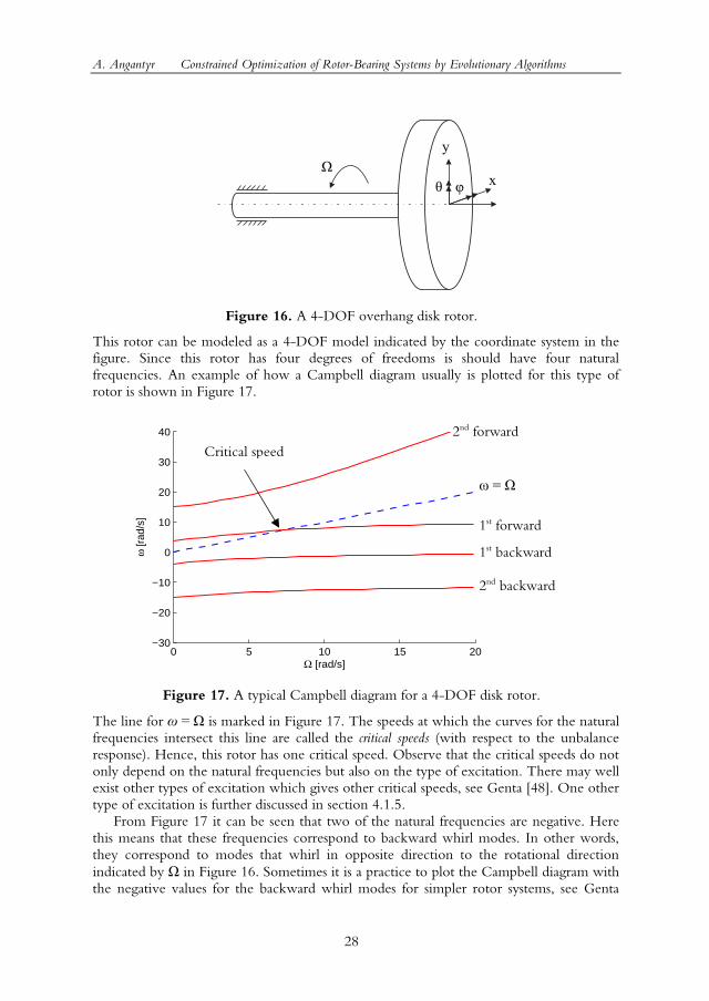
A. Angantyr Constrained Optimization of Rotor-Bearing Systems by Evolutionary Algorithms
28
Figure 16. A 4-DOF overhang disk rotor.
This rotor can be modeled as a 4-DOF model indicated by the coordinate system in the figure. Since this rotor has four degrees of freedoms is should have four natural frequencies. An example of how a Campbell diagram usually is plotted for this type of rotor is shown in Figure 17.
Figure 17. A typical Campbell diagram for a 4-DOF disk rotor.
The line for ω = Ω is marked in Figure 17. The speeds at which the curves for the natural frequencies intersect this line are called the critical speeds (with respect to the unbalance response). Hence, this rotor has one critical speed. Observe that the critical speeds do not only depend on the natural frequencies but also on the type of excitation. There may well exist other types of excitation which gives other critical speeds, see Genta [48]. One other type of excitation is further discussed in section 4.1.5. From Figure 17 it can be seen that two of the natural frequencies are negative. Here this means that these frequencies correspond to backward whirl modes. In other words, they correspond to modes that whirl in opposite direction to the rotational direction indicated by Ω in Figure 16. Sometimes it is a practice to plot the Campbell diagram with the negative values for the backward whirl modes for simpler rotor systems, see Genta
x
y
φ θΩ
0 5 10 15 20−30
−20
−10
0
10
20
30
40
Ω [rad/s]
ω [r
ad/s
]
1st forward
1st backward
2nd backward
ω = Ω
Critical speed 2nd forward
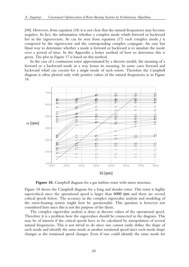
A. Angantyr Constrained Optimization of Rotor-Bearing Systems by Evolutionary Algorithms
29
[48]. However, from equation (18) it is not clear that the natural frequencies may become negative. In fact, the information whether a complex mode whirls forward or backward lies in the eigenvectors. As can be seen from equation (17) each complex mode j is composed by the eigenvector and the corresponding complex conjugate. An easy but blunt way to determine whether a mode is forward or backward is to simulate the mode over a period of time. In the Appendix a better method of how to determine this is given. The plot in Figure 17 is based on this method. In the case of a continuous rotor approximated by a discrete model, the meaning of a forward or a backward mode in a way looses its meaning. In some cases forward and backward whirl can coexist for a single mode of such rotors. Therefore the Campbell diagram is often plotted only with positive values of the natural frequencies as in Figure 18.
Figure 18. Campbell diagram for a gas turbine rotor with stator structure.
Figure 18 shows the Campbell diagram for a long and slender rotor. This rotor is highly supercritical since the operational speed is larger than 6000 rpm and there are several critical speeds below. The accuracy in the complex eigenvalue analysis and modeling of the rotor-bearing system might here be questionable. This question is however not considered here since this is not the purpose of the thesis. The complex eigenvalue analysis is done at discrete values of the operational speed. Therefore it is a problem how the eigenvalues should be connected in the diagram. This may be of interest if the critical speeds have to be calculated by interpolation of several natural frequencies. This is not trivial to do since one cannot easily define the shape of each mode and identify the same mode at another rotational speed since each mode shape changes as the rotational speed changes. Even if one could identify the same mode for
ω [rpm]
Ω [rpm]
1000 2000 3000 4000 5000 6000 7000 80001000
2000
3000
4000
5000
6000
7000
1 1 1 1 1 1
2 2 2 2 2 23
3 3 3 3 34
44 4 4 4
5
55 5 5 5
6
66 6 6 6
7
7 7 7 7 7
8
8
88
88
9
99 9
99
10
1010 10 10
10
11
11 11
11
11
11
12
12
1212 12
12
13
13 1313
13 13
14
1414 14
14
14
15
15 15 15 15 15
16
16 1616 16 16
17
17 17 17 17 17
18
18 18 18 18 18
19
19 19 19 19 19
20
20
20 20 20 20
21
21
21 21 21 21
22
22
22 22 22 22
23
23
23 23 23 23
24 24
24 24 24 24
2525
25 25 25 25
2626
26 26 26 2627 27
27 27 27 27
28 28
28 28 28 28
2929
29 29 29 29
30 30
3030 30 30
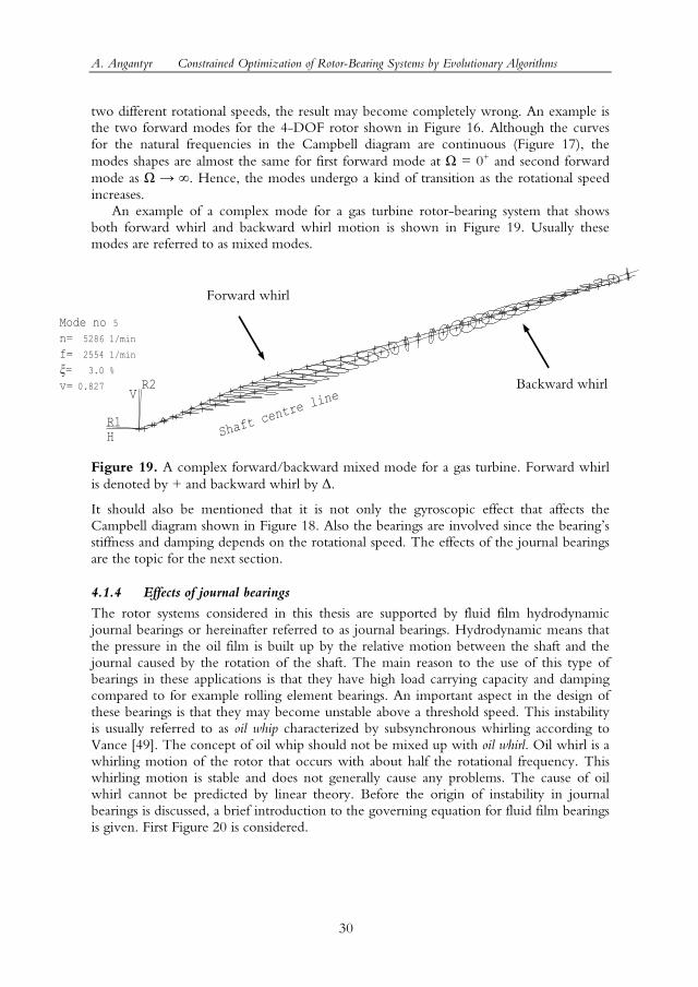
A. Angantyr Constrained Optimization of Rotor-Bearing Systems by Evolutionary Algorithms
30
two different rotational speeds, the result may become completely wrong. An example is the two forward modes for the 4-DOF rotor shown in Figure 16. Although the curves for the natural frequencies in the Campbell diagram are continuous (Figure 17), the modes shapes are almost the same for first forward mode at Ω = 0+ and second forward mode as Ω → ∞. Hence, the modes undergo a kind of transition as the rotational speed increases. An example of a complex mode for a gas turbine rotor-bearing system that shows both forward whirl and backward whirl motion is shown in Figure 19. Usually these modes are referred to as mixed modes.
Figure 19. A complex forward/backward mixed mode for a gas turbine. Forward whirl is denoted by + and backward whirl by ∆.
It should also be mentioned that it is not only the gyroscopic effect that affects the Campbell diagram shown in Figure 18. Also the bearings are involved since the bearings stiffness and damping depends on the rotational speed. The effects of the journal bearings are the topic for the next section.
4.1.4 Effects of journal bearings
The rotor systems considered in this thesis are supported by fluid film hydrodynamic journal bearings or hereinafter referred to as journal bearings. Hydrodynamic means that the pressure in the oil film is built up by the relative motion between the shaft and the journal caused by the rotation of the shaft. The main reason to the use of this type of bearings in these applications is that they have high load carrying capacity and damping compared to for example rolling element bearings. An important aspect in the design of these bearings is that they may become unstable above a threshold speed. This instability is usually referred to as oil whip characterized by subsynchronous whirling according to Vance [49]. The concept of oil whip should not be mixed up with oil whirl. Oil whirl is a whirling motion of the rotor that occurs with about half the rotational frequency. This whirling motion is stable and does not generally cause any problems. The cause of oil whirl cannot be predicted by linear theory. Before the origin of instability in journal bearings is discussed, a brief introduction to the governing equation for fluid film bearings is given. First Figure 20 is considered.
Backward whirl
Forward whirl
n=
f=
5286 1/min
2554 1/min
= 3.0 %
v= 0.827
Mode no 5
H
V
Shaft
centre
line
R1
R2
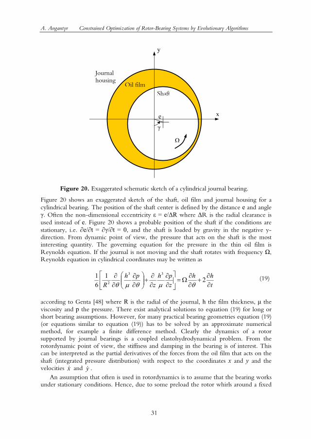
A. Angantyr Constrained Optimization of Rotor-Bearing Systems by Evolutionary Algorithms
31
Figure 20. Exaggerated schematic sketch of a cylindrical journal bearing.
Figure 20 shows an exaggerated sketch of the shaft, oil film and journal housing for a cylindrical bearing. The position of the shaft center is defined by the distance e and angle γ. Often the non-dimensional eccentricity ε = e/∆R where ∆R is the radial clearance is used instead of e. Figure 20 shows a probable position of the shaft if the conditions are stationary, i.e. ∂e/∂t = ∂γ/∂t = 0, and the shaft is loaded by gravity in the negative y-direction. From dynamic point of view, the pressure that acts on the shaft is the most interesting quantity. The governing equation for the pressure in the thin oil film is Reynolds equation. If the journal is not moving and the shaft rotates with frequency Ω, Reynolds equation in cylindrical coordinates may be written as
thh
zph
zph
R ∂∂
+∂∂
Ω=
∂∂
∂∂
+
∂∂
∂∂ 21
61 33
2 θµθµθ (19)
according to Genta [48] where R is the radial of the journal, h the film thickness, µ the viscosity and p the pressure. There exist analytical solutions to equation (19) for long or short bearing assumptions. However, for many practical bearing geometries equation (19) (or equations similar to equation (19)) has to be solved by an approximate numerical method, for example a finite difference method. Clearly the dynamics of a rotor supported by journal bearings is a coupled elastohydrodynamical problem. From the rotordynamic point of view, the stiffness and damping in the bearing is of interest. This can be interpreted as the partial derivatives of the forces from the oil film that acts on the shaft (integrated pressure distribution) with respect to the coordinates x and y and the velocities x& and y& . An assumption that often is used in rotordynamics is to assume that the bearing works under stationary conditions. Hence, due to some preload the rotor whirls around a fixed
x
y
Ω
Oil film Shaft
Journal housing
e
γ
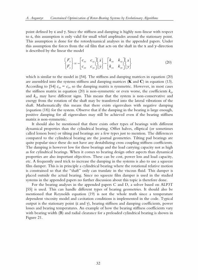
A. Angantyr Constrained Optimization of Rotor-Bearing Systems by Evolutionary Algorithms
32
point defined by ε and γ. Since the stiffness and damping is highly non-linear with respect to ε, this assumption is only valid for small whirl amplitudes around the stationary point. This assumption is done for the rotordynamical analyses in the appended papers. Under this assumption the forces from the oil film that acts on the shaft in the x and y-direction is described by the linear the model
−
−=
yx
kkkk
yx
cccc
FF
yyyx
xyxx
yyyx
xyxx
y
x
&
& (20)
which is similar to the model in [54]. The stiffness and damping matrices in equation (20) are assembled into the systems stiffness and damping matrices (K and C) in equation (13). According to [54] cxy = cyx so the damping matrix is symmetric. However, in most cases the stiffness matrix in equation (20) is non-symmetric or even worse, the coefficients kxy and kyx may have different signs. This means that the system is non-conservative and energy from the rotation of the shaft may be transferred into the lateral vibrations of the shaft. Mathematically this means that there exists eigenvalues with negative damping (equation (18)) for the system. Observe that if the damping in the bearing is large enough, positive damping for all eigenvalues may still be achieved even if the bearing stiffness matrix is non-symmetric. It should also be mentioned that there exists other types of bearings with different dynamical properties than the cylindrical bearing. Offset halves, elliptical (or sometimes called lemon bore) or tilting pad bearings are a few types just to mention. The differences compared to the cylindrical bearing are the journal geometries. Tilting pad bearings are quite popular since these do not have any destabilizing cross coupling stiffness coefficients. The damping is however low for these bearings and the load carrying capacity not as high as for cylindrical bearings. When it comes to bearing design other aspects than dynamical properties are also important objectives. These can be cost, power loss and load capacity, etc. A frequently used trick to increase the damping in the systems is also to use a squeeze film damper. This is in principle a cylindrical bearing where the rotational relative motion is constrained so that the shaft only can translate in the viscous fluid. This damper is placed outside the actual bearing. Since no squeeze film damper is used in the studied systems in the appended papers no further discussion about this topic is therefore done. For the bearing analyses in the appended papers C and D, a solver based on ALP3T [55] is used. This can handle different types of bearing geometries. It should also be mentioned that Reynolds equation (19) is not the whole truth since a temperature dependent viscosity model and cavitation conditions is implemented in the code. Typical output is the stationary point (ε and γ), bearing stiffness and damping coefficients, power losses and bearing temperatures. An example of how the bearing stiffness coefficients vary with bearing width (B) and radial clearance for a preloaded cylindrical bearing is shown in Figure 21.
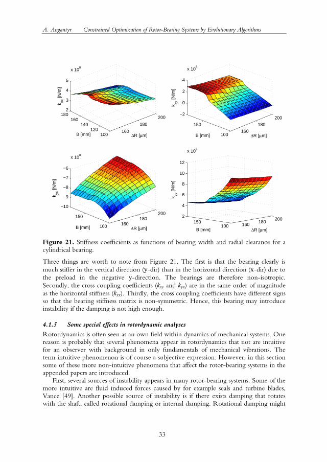
A. Angantyr Constrained Optimization of Rotor-Bearing Systems by Evolutionary Algorithms
33
160
180
200
100120
140160
1802
3
4
5
x 108
∆R [µm]B [mm]
k xx [N
/m]
160
180
200
100
150
−2
0
2
4
x 108
∆R [µm]B [mm]
k xy [N
/m]
160180
200
100
150
−10
−9
−8
−7
−6
x 108
∆R [µm]B [mm]
k yx [N
/m]
160180
200
100150
2
4
6
8
10
12
x 108
∆R [µm]B [mm]
k yy [N
/m]
Figure 21. Stiffness coefficients as functions of bearing width and radial clearance for a cylindrical bearing.
Three things are worth to note from Figure 21. The first is that the bearing clearly is much stiffer in the vertical direction (y-dir) than in the horizontal direction (x-dir) due to the preload in the negative y-direction. The bearings are therefore non-isotropic. Secondly, the cross coupling coefficients (kxy and kyx) are in the same order of magnitude as the horizontal stiffness (kxx). Thirdly, the cross coupling coefficients have different signs so that the bearing stiffness matrix is non-symmetric. Hence, this bearing may introduce instability if the damping is not high enough.
4.1.5 Some special effects in rotordynamic analyses
Rotordynamics is often seen as an own field within dynamics of mechanical systems. One reason is probably that several phenomena appear in rotordynamics that not are intuitive for an observer with background in only fundamentals of mechanical vibrations. The term intuitive phenomenon is of course a subjective expression. However, in this section some of these more non-intuitive phenomena that affect the rotor-bearing systems in the appended papers are introduced. First, several sources of instability appears in many rotor-bearing systems. Some of the more intuitive are fluid induced forces caused by for example seals and turbine blades, Vance [49]. Another possible source of instability is if there exists damping that rotates with the shaft, called rotational damping or internal damping. Rotational damping might
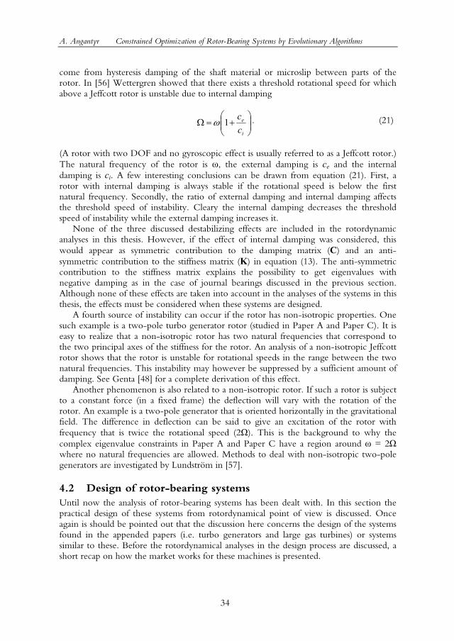
A. Angantyr Constrained Optimization of Rotor-Bearing Systems by Evolutionary Algorithms
34
come from hysteresis damping of the shaft material or microslip between parts of the rotor. In [56] Wettergren showed that there exists a threshold rotational speed for which above a Jeffcott rotor is unstable due to internal damping
+=Ω
i
e
cc1ω . (21)
(A rotor with two DOF and no gyroscopic effect is usually referred to as a Jeffcott rotor.) The natural frequency of the rotor is ω, the external damping is ce and the internal damping is ci. A few interesting conclusions can be drawn from equation (21). First, a rotor with internal damping is always stable if the rotational speed is below the first natural frequency. Secondly, the ratio of external damping and internal damping affects the threshold speed of instability. Cleary the internal damping decreases the threshold speed of instability while the external damping increases it. None of the three discussed destabilizing effects are included in the rotordynamic analyses in this thesis. However, if the effect of internal damping was considered, this would appear as symmetric contribution to the damping matrix (C) and an anti-symmetric contribution to the stiffness matrix (K) in equation (13). The anti-symmetric contribution to the stiffness matrix explains the possibility to get eigenvalues with negative damping as in the case of journal bearings discussed in the previous section. Although none of these effects are taken into account in the analyses of the systems in this thesis, the effects must be considered when these systems are designed. A fourth source of instability can occur if the rotor has non-isotropic properties. One such example is a two-pole turbo generator rotor (studied in Paper A and Paper C). It is easy to realize that a non-isotropic rotor has two natural frequencies that correspond to the two principal axes of the stiffness for the rotor. An analysis of a non-isotropic Jeffcott rotor shows that the rotor is unstable for rotational speeds in the range between the two natural frequencies. This instability may however be suppressed by a sufficient amount of damping. See Genta [48] for a complete derivation of this effect. Another phenomenon is also related to a non-isotropic rotor. If such a rotor is subject to a constant force (in a fixed frame) the deflection will vary with the rotation of the rotor. An example is a two-pole generator that is oriented horizontally in the gravitational field. The difference in deflection can be said to give an excitation of the rotor with frequency that is twice the rotational speed (2Ω). This is the background to why the complex eigenvalue constraints in Paper A and Paper C have a region around ω = 2Ω where no natural frequencies are allowed. Methods to deal with non-isotropic two-pole generators are investigated by Lundström in [57].
4.2 Design of rotor-bearing systems Until now the analysis of rotor-bearing systems has been dealt with. In this section the practical design of these systems from rotordynamical point of view is discussed. Once again is should be pointed out that the discussion here concerns the design of the systems found in the appended papers (i.e. turbo generators and large gas turbines) or systems similar to these. Before the rotordynamical analyses in the design process are discussed, a short recap on how the market works for these machines is presented.
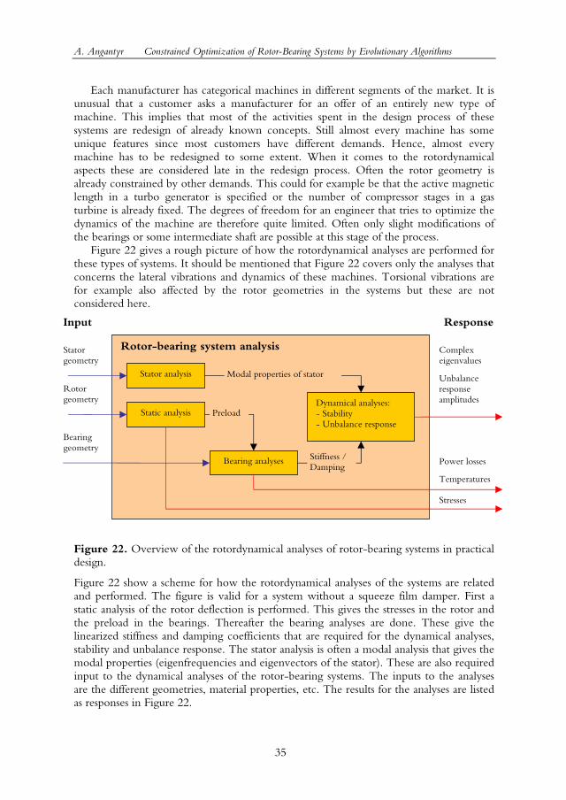
A. Angantyr Constrained Optimization of Rotor-Bearing Systems by Evolutionary Algorithms
35
Each manufacturer has categorical machines in different segments of the market. It is unusual that a customer asks a manufacturer for an offer of an entirely new type of machine. This implies that most of the activities spent in the design process of these systems are redesign of already known concepts. Still almost every machine has some unique features since most customers have different demands. Hence, almost every machine has to be redesigned to some extent. When it comes to the rotordynamical aspects these are considered late in the redesign process. Often the rotor geometry is already constrained by other demands. This could for example be that the active magnetic length in a turbo generator is specified or the number of compressor stages in a gas turbine is already fixed. The degrees of freedom for an engineer that tries to optimize the dynamics of the machine are therefore quite limited. Often only slight modifications of the bearings or some intermediate shaft are possible at this stage of the process. Figure 22 gives a rough picture of how the rotordynamical analyses are performed for these types of systems. It should be mentioned that Figure 22 covers only the analyses that concerns the lateral vibrations and dynamics of these machines. Torsional vibrations are for example also affected by the rotor geometries in the systems but these are not considered here.
Figure 22. Overview of the rotordynamical analyses of rotor-bearing systems in practical design.
Figure 22 show a scheme for how the rotordynamical analyses of the systems are related and performed. The figure is valid for a system without a squeeze film damper. First a static analysis of the rotor deflection is performed. This gives the stresses in the rotor and the preload in the bearings. Thereafter the bearing analyses are done. These give the linearized stiffness and damping coefficients that are required for the dynamical analyses, stability and unbalance response. The stator analysis is often a modal analysis that gives the modal properties (eigenfrequencies and eigenvectors of the stator). These are also required input to the dynamical analyses of the rotor-bearing systems. The inputs to the analyses are the different geometries, material properties, etc. The results for the analyses are listed as responses in Figure 22.
Rotor-bearing system analysis
Stator analysis
Static analysis
Bearing analyses
Dynamical analyses: - Stability - Unbalance response
Stator geometry
Rotor geometry
Bearing geometry
Input Response
Stresses
Power losses
Temperatures
Complex eigenvalues
Unbalance response amplitudes
Preload
Modal properties of stator
Stiffness / Damping
A. Angantyr Constrained Optimization of Rotor-Bearing Systems by Evolutionary Algorithms
36
Since the models and the results of the analyses contain errors, there must be some margins to the acceptable limits of the listed responses. These margins are usually defined in some design criteria. For the unbalance response there exist norms that not should be violated. However, a problem with the unbalance response is that the exact unbalance mass distribution is generally not known. In Paper D a set of unbalance cases is defined such that a reasonable unbalance (conservatively estimated from the known balancing grade) is placed at different positions. A possibility to avoid the problems with the unknown unbalance distribution might be to use the method based on singular value decomposition proposed by Cloud et al. in [58]. This approach overcomes this trouble and defines a general and conservative criterion that could be used for design purposes. A glance at Figure 22 probably gives the picture that rotordynamical design is about finding the optimal settings for some parameters subject to several objectives or constraints. In fact this is a common situation in the design of real rotor-bearing system design. Although the dynamical analyses are linear the mapping from input to responses in Figure 22 are expected to be all but linear. Since several objectives exists and the input parameters may be of several different types, it should hopefully be clear at this point that this is the area where optimization by EAs and rotordynamical analysis intersect each other: In the practical analysis for the late design of these machines.
A. Angantyr Constrained Optimization of Rotor-Bearing Systems by Evolutionary Algorithms
37
5 Summary of appended papers In this section short summaries of the appended papers are presented and finally the contribution from the author in each paper is given.
5.1 Paper A This paper presents an approach on how a real coded GA can be used in the design process of rotor-bearing systems in order to control the systems complex eigenvalues. The studied application is a turbo generator rotor-bearing system. The detailed design of a turbo generator rotor system is highly constrained by feasible regions for the complex eigenvalues of the system. A major problem for the designer is to find solutions that fulfill the design criterion for the complex eigenvalues (i.e. damping and damped natural frequencies). The bearing properties and geometrical parameters of the rotor are often used as the design parameters subjected to variations in order to search for feasible designs. This paper presents an alternative approach to be used at this stage of the design process. First the design criteria for several complex eigenvalues are reformulated in a scalar valued function that describes the degree of feasibility for a particular design. Then the search for feasible designs is formulated as an optimization problem and solved with a GA. Finally the problem is also extended to include another objective (i.e. multiobjective optimization) to show the potential of using the optimization formulation and a Pareto based GA in is rotordynamic application. The results show that the presented approach is promising as an engineering design tool. The scientific contribution of this paper is first how the complex eigenvalue design criteria are mapped on a scalar function that easily can be used to compare different designs. Secondly, the contribution is the multiobjective formulation that might inspire others working with similar kind of problems.
5.2 Paper B In this paper a new constraint handling technique for EAs is introduced. It is based on ideas from multiobjective optimization algorithms for GAs and it does not require any problem specific parameters to be set. Almost all practical design optimization problems are constrained by different reasons. A possible criticism of EAs is the lack of efficient and robust generic methods to handle constraints. The most widespread approach for constrained search problems is to use penalty methods. These methods often require that some extra penalty parameters have to be specified. The settings of these parameters are problem dependent and if the penalty functions are not designed properly, false optima may be introduced. During the last decade EAs have received increased interest in the field of multiobjective optimization. A constrained optimization problem or an unconstrained multiobjective problem may in principle be two different ways to pose the same underlying problem. Therefore it seems natural to glance at multiobjective EAs when algorithms for constrained optimization are designed. In this paper an alternative approach for the constrained optimization problem is presented. The method is a variant of a multiobjective real coded GA inspired by the penalty approach. It is evaluated on six
A. Angantyr Constrained Optimization of Rotor-Bearing Systems by Evolutionary Algorithms
38
different constrained single objective problems found in the literature. The result is compared to the result for other constraint handling techniques for GAs. The results show that the proposed method performs well in terms of efficiency, and that it is robust for a majority of the test problems. The contribution to the scientific and engineering community of this paper is a new and generic constraint handling method that can be used in many types of GAs.
5.3 Paper C This paper is a continuation of the work done in Paper A and the constraint handling technique developed in Paper B is used. In the design of large rotor-bearing systems such as steam turbines, gas turbines or generators, the whole rotor system should be optimal in some sense and simultaneously fulfill the design constraints. The bearing design has a crucial impact on the rotor system characteristics such as complex eigenvalues for example. In system optimizations it is therefore important to consider the bearing design. Until now the actual bearing geometry has seldom been used as design variables in system optimizations. In Paper A the uncoupled linearized bearing stiffness and damping coefficients where used as design variables. In this paper a bearing analysis code is included and the actual bearing geometry parameters are used as design variables. First, the generic constraint handling technique for GAs developed in Paper B is briefly explained. Then the optimization problem of a generator rotor-bearing system is formulated and solved by a real coded GA and the proposed method to handle the constraints. The objective is to minimize power loss subject to design specifications for bearing temperatures and complex eigenvalue constraints for the system. The result shows that a reduction of the power loss in the bearings may be achieved without violating the system design constraints. The result also shows how the design problem for a large rotor-bearing system can be handled. This is also the main scientific contribution in combination with the evaluation of the search methods performance on a difficult real-world design problem. To conclude, the paper shows a successful application of the presented search algorithm on an industrial rotor-bearing optimization problem.
5.4 Paper D This paper presents the optimization of the bearings design in a gas turbine rotor-bearing system. The effects taken into account are power loss and limiting temperatures in the bearings. The dynamics at the system level, i. e. stability and unbalances responses, are also considered. The design variables are the bearing widths and radial clearances. A real coded GA and constraint handling technique developed in Paper B is used. The problem formulation is specific for this particular design case but the used search method and outcome from the optimization is of general interest. The result is compared to the result of a nominal design. The result shows that it is most likely not possible to find a design that fulfills all the constraints for the system design. Still it is possible to find a design that gives a reduced power loss and does not violate any of the constraints more than the nominal design. The contribution to industry from this paper is that it gives a hint on how much slight modification of the bearings in large gas turbines may affect the rotor-bearing system performance. The scientific contribution is another reference of the performance of the constraint handling method in
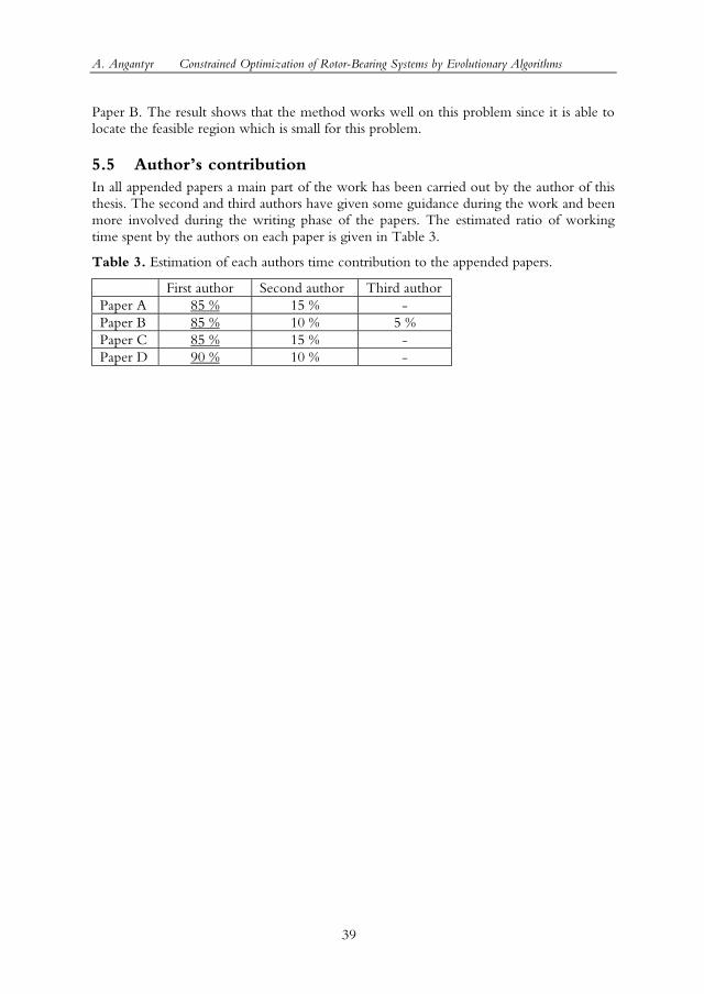
A. Angantyr Constrained Optimization of Rotor-Bearing Systems by Evolutionary Algorithms
39
Paper B. The result shows that the method works well on this problem since it is able to locate the feasible region which is small for this problem.
5.5 Authors contribution In all appended papers a main part of the work has been carried out by the author of this thesis. The second and third authors have given some guidance during the work and been more involved during the writing phase of the papers. The estimated ratio of working time spent by the authors on each paper is given in Table 3.
Table 3. Estimation of each authors time contribution to the appended papers.
First author Second author Third author Paper A 85 % 15 % - Paper B 85 % 10 % 5 % Paper C 85 % 15 % - Paper D 90 % 10 % -
A. Angantyr Constrained Optimization of Rotor-Bearing Systems by Evolutionary Algorithms
40
6 Discussion and future work In this section answers to research questions, some findings and experiences of this work are discussed. For more detailed conclusions the reader is referred to the appended papers.
6.1 Answer to research questions Paper A is a first attempt to answer the first research question at page 2. The design of a turbo generator rotor-bearing system is truly a multiobjective design problem when all objectives are considered. However, more work is necessary to fully answer this question. Important objectives such as costs and system robustness have for example not yet been properly addressed. Paper B to Paper D are attempts to answer the second research question at page 2. Paper B shows how multiobjective GAs can be adapted in order to solve a constrained optimization problem. Paper C and Paper D are examples of applications of EAs on real bearing design problems. The result in Paper D clearly shows that by the use of this method it is possible to improve the design compared with a nominal design. Therefore this shows that the used search method is able to find solutions that are better than what engineers yet have found. However, since no comparison to other methods is done one cannot conclude that this is the only possible way to find these results.
6.2 Importance of problem formulation From the experiences of this work it has become obvious that the problem formulation is important. With a very poor problem formulation the choice of search method does not matter. Hence, the results will probably be bad regardless of the choice of search method. However, with a moderately poor problem formulation the chance of finding successful results is probably better with EAs than most other methods. This since EAs are robust global search methods. From practical point of view this is important because the problem formulation is often more or less poor. Another fact worth to point out is that in order to achieve a good problem formulation, knowledge in the domain of search algorithms and the studied systems are required. Therefore it was also one purpose of this thesis, to bring some light into the intersection of these two domains.
6.3 Future work Optima where the solution is sensitive to perturbations in the design parameters are not desirable in real application. The post-optimal process is one subject that has not been addressed in this thesis. Therefore this is one area of future work. Population based methods such as GAs are interesting for this purpose since the design variables or other design parameters may be perturbed in the evolutionary process so that less robust solutions are rejected. Thereby only robust solutions are searched for. Another approach for further research is to study mixed variable problems. For example these arise in the design of rotor-bearing problems if different bearing types and other geometrical parameters are chosen as design variables. Binary design choices such as the possibility of a squeeze film damper or not is also imaginable. EAs are some of the
A. Angantyr Constrained Optimization of Rotor-Bearing Systems by Evolutionary Algorithms
41
more interesting methods for these types of problems since most other optimization techniques cannot handle mixed types of variables. A possible area in rotordynamical design where search and optimization methods can contribute is also in inverse modeling (or parameter identification). Inverse modeling is when some unknown parameters in a model are fit so that the model as closely as possible represents a real system. Uniqueness of solutions is a problem that frequently appears in inverse modeling. Niched GAs may be an approach to avoid these problems since niched GAs can search several local (or global) optima simultaneously in one single search. A field of rotor-bearing system design where the methods studied in this thesis are readily applicable is in service and retrofit applications. In these contexts the design problems are quite easily formulated and the number of possible design variables is restricted to only a few, for example bearing geometry parameters. Still it is of importance to find an optimal design or a Pareto optimal design.
A. Angantyr Constrained Optimization of Rotor-Bearing Systems by Evolutionary Algorithms
42
7 References [1] Rajan, M., Rajan, S. D., Nelson, H. D. and Chen, W. J., 1987, Optimal
Placement of Critical Speeds in Rotor-Bearing Systems, ASME Journal of Vibration Acoustics, Stress, and Reliability in Design, 109, pp. 152-157.
[2] Steffen Jr, V., Pacheco, R P. and Borges, J. A. F, 1997, Optimization Techniques in Rotordynamics, Proceedings of the 15th International Modal Analysis Conference, Orlando, FL, USA, pp. 2009-2015.
[3] Srinivasan, S., Maslen, E. H. and Barret, L. E., 1997, Optimization of Bearing Locations for Rotor Systems with Magnetic Bearings, ASME Journal of Engineering for Gas Turbines and Power, 119, pp. 464-468.
[4] Shiau, T. N., Kuo C. P. and Hwang, J. R., 1994, Multiobjective Optimization of a Flexible Rotor in Magnetic Bearings with Critical Speeds and Control Current Constraints, Proceedings of the International Gas Turbine Aeroengine Congress and Exposition, ASME, New York, NY, pp. 1-13.
[5] Lee, D. S. and Choi, D. H., 2000, Reduced Weight Design of a Flexible Rotor with Ball Bearing Stiffness Characteristics Varying with Rotational Speed and Load, ASME Journal of Vibration and Acoustics, 122, pp. 203-208.
[6] Montusiewicz, J. and Osyczka A., 1997, Computer aided optimum design of machine tool spindle systems with hydrostatic bearings, Journal of Engineering Manufacture, 211, pp. 43-51.
[7] Doizelet, D. and Bondoux, D. 1990, Application of Optimization Techniques for Hypercritical Rotors, Proceedings of the 3rd International Conference on Rotor Dynamics, Lyon, pp. 57-62.
[8] Diewald, W. and Nordmann, R., 1990, Parameter Optimization for the Dynamics of Rotating Machinery, Proceedings of the 3rd International Conference on Rotor Dynamics, Lyon, pp. 51-55.
[9] Chen, T. Y. and Wang, B. P., 1993, Optimum Design of Rotor-Bearing Systems with Eigenvalue Constraits, ASME Journal of Engineering for Gas Turbines and Power, 115, pp. 256-260.
[10] Shiau, T. N. and Chang, J. R., 1993, Multi-objective Optimization of Rotor-Bearing System With Critical Speed Constraits, ASME Journal of Engineering for Gas Turbines and Power, 115, pp. 246-255.
[11] Genta, G. and Bassani, D., 1995, Use of Genetic Algorithms for the Design of Rotors, Meccanica, 30, pp. 707-717.
[12] Choi, B.-K. and Yang, B.-S., 2001, Optimal Design of Rotor-Bearing Systems Using Immune-Genetic Algorithm, ASME Journal of Vibration and Acoustics, 123, pp. 398-401.
A. Angantyr Constrained Optimization of Rotor-Bearing Systems by Evolutionary Algorithms
43
[13] Choi, B.-K. and Yang, B.-S., 2001, Multiobjective Optimum Design of Rotor-Bearing Systems With Dynamic Constraints Using Immune-Genetic Algorithm, ASME Journal of Engineering for Gas Turbines and Power, 123, pp. 78-81.
[14] Choi, B.-G. and Yang, B.-S., 2000, Optimum Shape Design of Rotor Shafts Using Genetic Algorithm, ASME Journal of Vibration and Control, 6, pp. 207-222.
[15] Choi, S.-P., Kim, Y.-C. and Yang, B.-S., 2002, Optimum Design of Rotor-Bearing System using Advanced Genetic Algorithm, Proceedings of the 9th International Symposium on Transport Phenomena and Dynamics of Rotating Machinery, Honolulu, Hawaii.
[16] Roark, R. J. and Young, W. C., 1975, Formulas for Stress and Strain, McGraw-Hill, New-York.
[17] Onwubiko, Chinyere, 2000, Introduction to Engineering Design Optimization, Prentice-Hall, New Jersey.
[18] Andersson, J., 2001, Multiobjective Optimization in Engineering Design, PhD thesis No. 675, Linköping University, Linköping.
[19] Deb, Kalyanmoy, 2002, Multi-Objective Optimization using Evolutionary Algorithms, John Wiley and Sons, New York.
[20] Montgomery, Douglas C., 2001, Design and Analysis of Experiments, John Wiley and Sons, New York.
[21] Rao, S., 1996, Engineering Optimization: Theory and Practice, John Wiley and Sons, New York.
[22] Venter, G., Hajtka, R. T. and Starner, J. Jr., 1996, Construction of Response Surfaces for Design Optimization Applications, Proceedings of the AIAA/NASA/USAF/ISSMO 6th Conference on Multidiciplinary Analysis and Optimization (Bellevue, WA), AIAA, Reston, VA, pp. 548-564.
[23] Hajelea, P. and Lee, J., 1996, Role of Emergent Computing Techniques in Multidisciplinary Design, In Grierson D. and Hajela P. (Eds.), Proceedings of the NATO Advanced Research Workshop in Emergent Computing Methods in Engineering Design (Nafplio, Greece), Springer-Verlag, Berlin, pp. 162-187.
[24] Hajela, P., 1999, Nongradient Methods in Multidisciplinary Design Optimization Status and Potential, Journal of Aircraft, 36(1), pp. 255-265.
[25] Box, M. J., 1965, A new method of constraint optimization and comparison with other methods, Computer Journal, 8, pp. 42-52.
[26] Kirkpatrick, S., Gellat, C. D. Jr. and Vecchi, M. P., 1983, Optimization by Simulated Annealing, Science, 220(4598), pp. 671-680.
[27] Holland, H. J., 1975, Adaptation in Natural and Artificial Systems, an Introductory Analysis with Application to Biology, Control and Artificial Intelligence, The University of Michigan Press, Ann Arbor, USA.
A. Angantyr Constrained Optimization of Rotor-Bearing Systems by Evolutionary Algorithms
44
[28] Rechenberg, I., 1973, Evolutionsstrategie Optimierung technischer Systeme nach Prinzipien der biologischen Evolution, Friedrich Frommann Verlag, Stuttgart.
[29] Goldberg, D. E., 1989, Genetic Algorithms in Search, Optimization and Machine Learning, Addison-Wesley, Reading.
[30] Davis, L. (Ed.), 1991, Handbook of Genetic Algorithms, Van Nostrand Reinhold, New York.
[31] Gen, M. and Cheng, R., 2000, Genetic Algorithms & Engineering Optimization, John Wiley and Sons, New York.
[32] Bäck, T. and Hoffmeister, 1991, "Extended Selection Mechanisms in Genetic Algorithms", In Belew R. K. and Booker L. B. (Eds.), Proceedings of the Fourth International Conference on Genetic Algorithms, San Mateo, California, Morgan Kaufmann Publishers, pp. 92-99.
[33] Goldberg, D. E. and Deb, K., 1991, A Comparative Analysis of Selection Schemes Used in Genetic Algorithms, In Rawlins G. J. E. (Ed.), Foundations of Genetic Algorithms. San Mateo, California, Morgan Kaufmann Publishers, pp. 69-93.
[34] Baker, J. E., 1987, Reducing Bias and Inefficiency in the Selection Algorithm, In Grefenstette J. J. (Ed.), Proceedings of the Second International Conference on Genetic Algorithms and their Application, Hillsdale, New Jersey, Lawrence Erlbaum Associates, pp. 14-21.
[35] Deb, K. and Agrawal, R. B., 1995, Simulated Binary Crossover for Continuous Search Space, Complex Systems, 9(2), pp. 115-148.
[36] Eshelman L. J. and Schaffer J. D., 1993, Real-Coded Genetic Algorithms and Interval-Schemata, In L. D. Whitley (Ed.), Foundations of Genetic Algorithms 2, Morgan Kaufmann, San Mateo, CA, pp. 187-202.
[37] Mühlenbein, H. and Schlierkamp-Voosen, D., 1993, Predictive Models for the Breeder Genetic Algorithm: I. Continuous Parameter Optimization, Evolutionary Computation, 1 (1), pp. 25-49.
[38] Herrara, F., Lozano, M. and Verdegay, J. L., 1998, Tackling real-coded genetic algorithms: Operators and tools for behavioral analysis, Artificial Intelligence Review, 12(4), pp. 265-319.
[39] Andersson, J., 2000, A Survey of Multiobjective Optimization in Engineering Design, Technical Report No. LiTH-IKP-R-1097, Linköping University, Linköping.
[40] Fonseca, C. M. and Fleming, P. J., 1993, Genetic Algorithms for Multiobjective Optimization: Formulation, Discussion and Generalization, Proceedings of the 5th International Conference on Genetic Algorithms, Morgan Kaufmann Publishers, San Francisco, pp. 416-423.
A. Angantyr Constrained Optimization of Rotor-Bearing Systems by Evolutionary Algorithms
45
[41] Deb, K., Pratap, A., Agarwal, S. and Meyarivan, T., 2000, A Fast and Elitist Multi-Objective Genetic Algorithm: NSGA-II, KanGAL Report No. 200001, Kanpur Genetic Algorithm Laboratory, Kanpur.
[42] Coello Coello, C. A., 2002, Theoretical and numerical constraint-handling techniques used with evolutionary algorithms: a survey of state of the art, Computer methods in applied mechanics and engineering, 191, pp. 1245-1287.
[43] Richardson, J. T., Palmer, M. R., Liepins, G. and Hilliard ,M., 1989, Some Guidelines for Genetic Algorithms with Penalty Functions, In J. D. Schaffer (Ed.), Proceedings of the 3rd International Conference on Genetic Algorithms, Morgan Kaufmann, Reading, MA, pp. 191-197.
[44] Michalewicz, Z., 1995, Genetic Algorithms, Numerical Optimization, and Constraints, In L. Eshelman (Ed.), Proceedings of the 6th International Conference on Genetic Algorithms, Morgan Kaufmann, San Francisco, pp. 151-158.
[45] Coello Coello, C. A., 1999, A Survey of Constraint Handling Techniques used with Evolutionary Algorithms, Technical Report Lania-RI-99-04, Laboratorio Nacional de Informática Avanzada, Xalapa.
[46] Michalewicz, Z., 1995, A Survey of Constraint Handling Techniques in Evolutionary Computation Methods, In J. R. McDonnell, R. G. Reynolds and D. B. Fogel (Eds.), Proceedings of the 4th Annual Conference on Evolutionary Programming, MIT Press, Cambridge, MA, pp. 135-155.
[47] Fonseca, C. M. and Fleming, P. J, 1995, Multiobjective Optimization and Multiple Constraint Handling with Evolutionary Algorithms I: A Unified Formulation, Research Report 564, University of Sheffield, Sheffield.
[48] Genta, G., 1999, Vibration of Structures and Machines, Spinger-Verlag, New York.
[49] Vance, J. M., 1988, Rotordynamics of Turbomachinery, John Wiley and Sons, New York.
[50] Meirovitch, L., 2001, Fundamentals of Vibrations, McGraw-Hill, New York.
[51] Cook, R. D., Malkus, D. S. and Plesha, M. E., 1989, Concepts and applications of finite element analysis, John Wiley and Sons, New York.
[52] Nelson, H. D. and McVaugh, J. M., 1976, The Dynamics of Rotor-Bearing Systems Using Finite Elements, Journal of Engineering for Industry, 98, pp. 593-600.
[53] Inman, D. J., 2001, Engineering Vibration, Prentice Hall, New Jersey.
[54] Olsson, K.-O. and Wettergren, H., 2000, Maskindynamik, Studentlitteratur, Lund, Sweden.
[55] Mittwollen, N. and Glienicke, J., 1990, Operating Conditions of Multi-Lobe Journal Bearings Under High Thermal Loads, ASME Journal of Tribology, 112, pp. 330-340.
A. Angantyr Constrained Optimization of Rotor-Bearing Systems by Evolutionary Algorithms
46
[56] Wettergren, H., 1996, Rotordynamic Analysis with Special Reference to Composite Rotors and Internal Damping, PhD thesis No. 464, Linköping University, Linköping.
[57] Lundström, M., 2002, Laffoon slits: a method to compensate unsymmetrical rotor bending stiffness, Master thesis No. 066, Luleå University of Technology, Luleå.
[58] Cloud, C. H., Foiles, W. C., Li, G., Maslen, E. H. and Barret, L. E., 2002, Practical applications of singular value decomposition in rotordynamics, In E. J. Hahn and R. B. Randall (Eds.), Proceedings of the Sixth International Conference on Rotor Dynamics, UNSW Printing Services, Sydney, Australia, 1, pp. 429-438.
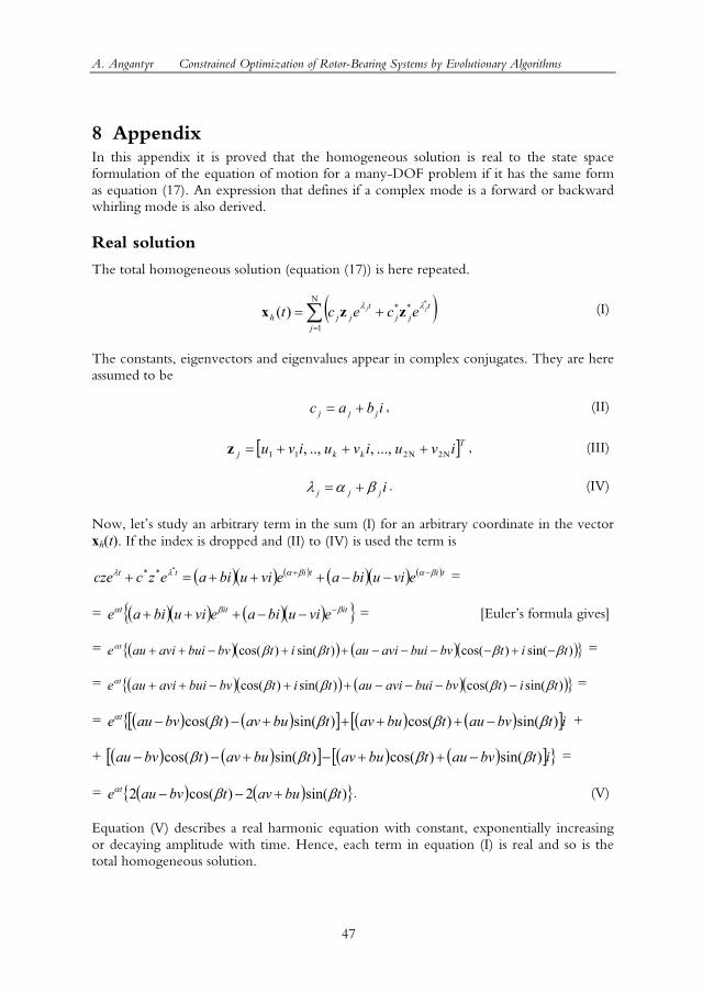
A. Angantyr Constrained Optimization of Rotor-Bearing Systems by Evolutionary Algorithms
47
8 Appendix In this appendix it is proved that the homogeneous solution is real to the state space formulation of the equation of motion for a many-DOF problem if it has the same form as equation (17). An expression that defines if a complex mode is a forward or backward whirling mode is also derived.
Real solution
The total homogeneous solution (equation (17)) is here repeated.
( )∑=
+=N
1
** *
)(j
tjj
tjjh
jj ecect λλ zzx (I)
The constants, eigenvectors and eigenvalues appear in complex conjugates. They are here assumed to be
ibac jjj += , (II)
[ ]Tkkj ivuivuivu N2N211 ...,,..,, +++=z , (III)
ijjj βαλ += . (IV)
Now, lets study an arbitrary term in the sum (I) for an arbitrary coordinate in the vector xh(t). If the index is dropped and (II) to (IV) is used the term is
( )( ) ( ) ( )( ) ( )tititt eviubiaeviubiaezccze βαβαλλ −+ −−+++=+*** =
= ( )( ) ( )( ) ititt eviubiaeviubiae ββα −−−+++ = [Eulers formula gives]
= ( )( ) ( )( ) )sin()cos()sin()cos( titbvbuiaviautitbvbuiaviaue t ββββα −+−−−−++−++ =
= ( )( ) ( )( ) )sin()cos()sin()cos( titbvbuiaviautitbvbuiaviaue t ββββα −−−−++−++ =
= ( ) ( )[ ] ( ) ( )[ ]itbvautbuavtbuavtbvaue t )sin()cos()sin()cos( ββββα −++++−− +
+ ( ) ( )[ ] ( ) ( )[ ] itbvautbuavtbuavtbvau )sin()cos()sin()cos( ββββ −++−+−− =
= ( ) ( ) )sin(2)cos(2 tbuavtbvaue t ββα +−− . (V)
Equation (V) describes a real harmonic equation with constant, exponentially increasing or decaying amplitude with time. Hence, each term in equation (I) is real and so is the total homogeneous solution.
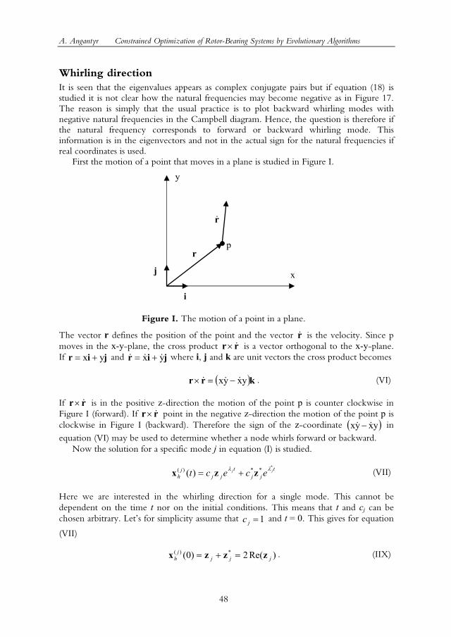
A. Angantyr Constrained Optimization of Rotor-Bearing Systems by Evolutionary Algorithms
48
Whirling direction It is seen that the eigenvalues appears as complex conjugate pairs but if equation (18) is studied it is not clear how the natural frequencies may become negative as in Figure 17. The reason is simply that the usual practice is to plot backward whirling modes with negative natural frequencies in the Campbell diagram. Hence, the question is therefore if the natural frequency corresponds to forward or backward whirling mode. This information is in the eigenvectors and not in the actual sign for the natural frequencies if real coordinates is used. First the motion of a point that moves in a plane is studied in Figure I.
Figure I. The motion of a point in a plane.
The vector r defines the position of the point and the vector r& is the velocity. Since p moves in the x-y-plane, the cross product rr &× is a vector orthogonal to the x-y-plane. If jir yx += and jir yx &&& += where i, j and k are unit vectors the cross product becomes
( )krr yxyx &&& −=× . (VI)
If rr &× is in the positive z-direction the motion of the point p is counter clockwise in Figure I (forward). If rr &× point in the negative z-direction the motion of the point p is clockwise in Figure I (backward). Therefore the sign of the z-coordinate ( )yxyx && − in equation (VI) may be used to determine whether a node whirls forward or backward. Now the solution for a specific mode j in equation (I) is studied.
tjj
tjj
jh
jj ecect***)( )( λλ zzx += (VII)
Here we are interested in the whirling direction for a single mode. This cannot be dependent on the time t nor on the initial conditions. This means that t and cj can be chosen arbitrary. Lets for simplicity assume that 1=jc and t = 0. This gives for equation
(VII)
)Re(2)0( *)(jjj
jh zzzx =+= . (IIX)
r&
r
x
y
i
j
p
A. Angantyr Constrained Optimization of Rotor-Bearing Systems by Evolutionary Algorithms
49
From equation (IIX) it is possible to identify the position (r) and velocity (r& ) for a single node (the point p in Figure I) for mode j at time t = 0. Then the sign of ( )yxyx && − can be used to determine the whirling direction.


