arX

iv:1

205.

1613

v1 [

astr

o-ph

.CO

] 8

May

201

2

Constraining massive gravity with recent cosmological data

Vincenzo F. Cardone∗

I.N.A.F. -Osservatorio Astronomico di Roma, via Frascati 33, 00040 - Monte Porzio Catone (Roma), Italy

Ninfa Radicella†

Departamento de Fısica, Universitat Autonoma de Barcelona, 08193 Bellaterra (Barcelona), Spain

Luca Parisi‡

Dipartimento di Fisica “E.R. Caianiello”, Universita di Salerno and I.N.F.N. - Sez. di Napoli - GC di Salerno,Via Ponte Don Melillo, 84084 Fisciano (Sa), Italy

A covariant formulation of a theory with a massive graviton and no negative energy state has beenrecently proposed as an alternative to the usual General Relativity framework. For a spatially flathomogenous and isotropic universe, the theory introduces modified Friedmann equations where thestandard matter term is supplemented by four effective fluids mimicking dust, cosmological constant,quintessence and stiff matter, respectively. We test the viability of this massive gravity formulationby contrasting its theoretical prediction to the Hubble diagram as traced by Type Ia Supernovae(SNeIa) and Gamma Ray Bursts (GRBs), the H(z) measurements from passively evolving galaxies,Baryon Acoustic Oscillations (BAOs) from galaxy surveys and the distance priors from the CosmicMicrowave Background Radiation (CMBR) anisotropy spectrum. It turns out that the model isindeed able to very well fit this large dataset thus offering a viable alternative to the usual darkenergy framework. We finally set stringent constraints on its parameters also narrowing down theallowed range for the graviton mass.

PACS numbers: 04.50.Kd, 98.80.-k

I. INTRODUCTION

There is a limited but crucial number of cosmologicalevidences which does not fit in the scheme constituted byGeneral Relativity (GR) and the Standard Model of par-ticle physics. On the one hand, it seems that the amountof baryonic matter in galaxies and galaxy clusters is notsufficient to cause the observed behaviour of the gravita-tional field on those scales. On the other hand, recentdata on the SNeIa Hubble diagram provide evidencesfor an accelerated expansion, also confirmed by severalother independent cosmological observations [1, 2]. Sucha large dataset can be very well reproduced by the con-cordance ΛCDM model made out of cold dark matter(CDM) and cosmological constant Λ. Notwithstandingthis remarkable success, the ΛCDM scenario is theoreti-cally unappealing since it comprises two exotic mattersources, namely dark energy and dark matter, and ismoreover plagued by several well known shortcomings.

A different constructive point of view is to addressthese problems introducing modifications of GR overlarge distances in order to possibly explain our ignoranceabout the 95% of the energy and matter content of theUniverse. In this setting, a massive deformation of GR isa plausible modified theory of gravity that is both phe-nomenologically and theoretically intriguing.

∗Electronic address: winnyenodrac@gmail.com†Electronic address: ninfa.radicella@uab.cat‡Electronic address: parisi@sa.infn.it

From the theoretical point of view, a small nonvanish-ing graviton mass is an open issue. The idea was origi-nally introduced in the work of Fierz and Pauli [3], whoconstructed a massive theory of gravity in a flat back-ground that is ghost - free at the linearized level. Sincethen, a great effort has been put in extending the result atthe nonlinear level and constructing a consistent theory.As a somewhat unanticipated result, we nowadays recog-nize that such models can be relevant for cosmology tooas possible alternative candidates to drive the acceleratedexpansion without the need of any exotic component.

Here we study cosmological solutions in the frame-work of a covariant massive gravity model, recently pro-posed in [4, 5]. At the linearized order, the mass termbreaks the gauge invariance of GR. Moreover, in orderto construct a consistent theory, nonlinear terms shouldbe tuned to remove order by order the negative energystate in the spectrum [6]. The theoretical model underinvestigation follows from a procedure originally outlinedin [7, 8] and has been found not to show ghosts at leastup to quartic order in the nonlinearities [9, 10].

We focus on cosmological equations of such theory,considering a spatially flat Robertson -Walker (RW)model in presence of both matter and radiation. Dueto the potential term, four new terms are present in theFriedmann equations mimicking dust, cosmological con-stant, quintessence and stiff matter. The presence of thecosmological constant and quintessence - like terms easilysuggest the possibility to achieve an accelerated expan-sion, while the stiff matter one can guarantee the haltingof the cosmic speed up in the intermediate redshift regimethus recovering the standard decelerating matter domi-

2

nated epoch. In order to check whether this is indeedthe case, we contrast the model predictions with a widedataset thus also being able to constrain its parameters.As a side effect, this will also allow us to narrow downthe range for the graviton mass.The plan of the paper is as follows. Sect. II presents

the basics of the theory and put down the modified Fried-mann equations describing the background cosmic evo-lution. The data we use and some subtleties specific tothe massive gravity framework are discussed in Sect. III,while the results of the likelihood analysis and the con-straints on the massive gravity coupling quantities aregiven in Sect. IV. We finally summarize and highlightsome important issues in the concluding Sect. V.

II. MASSIVE GRAVITY

Let us consider a four dimensional manifold equippedwith both a dynamical metric gµν and a non - dynamicalflat metric fµν . In order to determine the dynamics onthis structure, the starting point is to consider the fol-lowing action1 [11]

S = − 1

8πG

∫(

1

2R+m2U

)

d4x+ SM (1)

where G is the Newton coupling constant, R the Ricciscalar for gµν , U the potential, and SM describes ordinarymatter which is supposed to directly interact only withgµν . The potential term, coupled through the gravitonmass m, is given by

U =1

2

(

K2 −KνµKµ

ν

)

+c33!ǫµνρσǫ

αβγσKµαKν

βKργ

+c44!ǫµνρσǫ

αβγδKµαKν

βKργKσ

δ , (2)

with ǫµνρσ the Levi - Civita symbol, while the field K isrelated to the flat metric fµν through

Kµν = δµν − γµ

ν ,

and we have defined

γµσγ

σν = gµσfσν .

The theory is fully assigned by the graviton mass mg =~m/c and the two coupling parameters (c3, c4).In order to derive the cosmological equations, one has

to insert the RW metric into the field equations obtainedby the usual variational approach to the action (1) andimpose the constraints dictated by the Bianchi identities

1 Unless otherwise specified, we will set the speed of light c = 1.

[5]. For generic values of the (c3, c4) couplings and aspatially flat universe consistent with CMBR data [12],the expansion rate turns out to be [13]

3H2

8πG= ρM (a) + ρr(a)

+ m2(4c3 + c4 − 6)

+3m2β(3− 3c3 − c4)

a

+3m2β2(c4 + 2c3 − 1)

a2

− m2β3(c3 + c4)

a3, (3)

where a is the scale factor, H = a/a the usual Hubble pa-rameter (with the dot denoting derivative with respect tocosmic time), m2 = (m2c2)/(8πG) and we have assumeda source term made out by dust (M) and radiation (r).Since matter is assumed to be minimally coupled to grav-ity only, its conservation equation will be the usual

ρi + 3H(ρi + pi) = 0 (4)

with pi = 0 (pi = ρr/3) for i = M (i = r). Introducingthe redshift z = 1/a − 1, we can therefore convenientlyrewrite Eq.(3) as

E2(z) = ΩeffΛ +Ωeff

Q (1 + z) + ΩeffS (1 + z)2

+ ΩeffM (1 + z)3 +Ωr(1 + z)4 (5)

with E(z) = H(z)/H0 (the label 0 denoting present dayvalues), Ωi the standard present day density parameterfor the component i, while we have defined the effectivedensity parameters for the massive gravity terms as

ΩeffΛ = µ2(4c3 + c4 − 6)

ΩeffQ = 3µ2β(3 − 3c3 − c4)

ΩeffS = 3µ2β2(c4 + 2c3 − 1)

ΩeffM = ΩM − m2β3(c3 + c4)

, (6)

with µ2 = m2/ρcrit and ρcrit = 3H20/8πG the present

day critical density2. Note that the (c3, c4, β) parametersentering Eq.(3) are all dimensionless.A look at Eq.(5) shows that a massive graviton has a

double effect on the Hubble rate. First, as is somewhatexpected, it changes the matter content shifting the dust

2 Note that, since m = cmg/~, it has the dimension of (length)−1

so that µ2 = (m2c2)/(3H2

0) is dimensionless.

3

density parameter from the usual ΩM value to the effec-

tive one ΩeffM . It is, however, worth stressing that, since

the sign of c3 + c4 is not set from the theory, it is alsopossible that the effective matter content is smaller thanthe actual one. Actually, the most interesting feature is

the presence of the three further terms (ΩeffΛ ,Ωeff

Q ,ΩeffS )

mimicking a cosmological constant, a quintessence - likefield and stiff matter, respectively. Depending on the val-ues of (c3, c4) and the graviton mass, it is therefore pos-sible to reproduce the expected series of radiation domi-nation, matter era and accelerating expansion (driven by

both ΩeffΛ

and ΩeffQ ) with only a small contribute from

the unusual stiff matter term. It is this particular featurethat makes massive gravity so appealing from a cosmo-logical point of view motivating the present analysis.

In order to constrain the model parameters, it is actu-ally more convenient to replace the effective density pa-rameters with w0 = weff (z = 0) and wp = dweff/dz|z=0

with weff the equation of state (EoS) of the effectivedark energy model having the same Hubble parameterthan the massive gravity one. This quantity is defined as

weff (z) = −1 +

[

2

3

d lnE(z)

d ln (1 + z)

− ΩeffM (1 + z)3

E2(z)− Ωr(1 + z)4

E2(z)

]

×[

1− ΩeffM (1 + z)3

E2(z)− Ωr(1 + z)4

E2(z)

]−1

(7)

so that, by using Eq.(5), we get

weff (z) = −

3[

ΩeffΛ +Ωeff

Q (1 + z) + ΩeffS (1 + z)2

]−1

×[

3ΩeffΛ

+ 2ΩeffQ (1 + z)

+ ΩeffS (1 + z)2 − Ωr(1 + z)4

]

. (8)

Imposing now E2(z = 0) = 1, w0 = weff (z = 0) andwp = dweff/dz|z=0, it is only a matter of algebra to get

ΩeffΛ =

9

2(1 − Ωeff

M − Ωr)w20

+3

2(3 − 3Ωeff

M − 4Ωr)w0

+3

2(1 − Ωeff

M − Ωr)wp

+ (1− ΩeffM − 3Ωr) , (9)

ΩeffS =

9

2(1− Ωeff

M − Ωr)w20

+3

2(5− 5Ωeff

M − 6Ωr)w0

+3

2(1− Ωeff

M − Ωr)wp

+ 3(1− ΩeffM − 2Ωr) , (10)

ΩeffQ = 1− Ωeff

Λ− Ωeff

S − ΩeffM − Ωr . (11)

Using these relations, we can conveniently parameterizethe model in terms of the effective matter density pa-

rameter ΩeffM and the present day values of the effective

EoS and its derivative (w0, wp). It is worth stressing

that, depending on (ΩeffM ,Ωγ , w0, wp) combinations, it is

possible that some of the (ΩeffΛ

,ΩeffQ ,Ωeff

S ) parameterstake a negative value. This is, however, not a problem

since (ΩeffΛ ,Ωeff

Q ,ΩeffS ) refer to effective fluids, not ac-

tual ones. This can also be seen from Eqs.(6) which show

that negative Ωeffi can indeed be obtained depending on

the values of the massive gravity couplings (c3, c4).

III. MASSIVE GRAVITY VS DATA

Eq.(8) shows that the massive gravity introduces aneffective dark energy fluid whose EoS has the right be-haviour to drive cosmic acceleration. Indeed, should the

ΩeffΛ term be the dominant at low z, we get weff (z <<

1) ≃ −1 so that a ΛCDM- like expansion is obtained inthe late universe. As z increases, we can still have an

accelerated expansion as far as ΩeffQ dominates leading

to weff (z) ≃ −2/3 in the intermediate redshift regime,while the transition to a decelerating epoch is guaran-

teed by the stiff matter term ΩeffS . These encouraging

features have to substantiated by the comparison withthe available data which can both validate the model andconstrain its parameters.Although the dataset we are going to use is a typical

one, there are some subtleties specific of the massive grav-ity framework which require some caution. We thereforeprefer to spend some words to describe how we comparethe model to the each kind of dataset.

A. Hubble diagram

A first step in testing any proposed model is the com-parison with the Hubble diagram, i.e. the distance mod-ulus µ as a function of the redshift z. This is related tothe Hubble parameter E(z) as

µ = 25 + 5 log dL(z,p) (12)

4

with

dL(z,p) = (1 + z)r(z,p) (13)

the luminosity distance and

r(z,p) =c

H0

∫ z

0

dz′

E(z′,p)(14)

the comoving distance. Note that we have collectivelydenoted with p the set of model parameters.A classical tracer of the Hubble diagram is represented

by SNeIa so that we use the Union2 dataset [14] compris-ing NSNeIa = 557 objects tracing the Hubble diagramover the redshift range (0.015, 1.4). The correspondinglikelihood term will read :

LSNeIa =1

(2π)NSNeIa |CSNeIa|1/2(15)

× exp

[

−DTSNeIa(p)C

−1SNeIaDSNeIa(p)

2

]

with CSNeIa the SNeIa covariance matrix and D(p) aNSNeIa - dimensional vector with the i - th element givenby µobs(zi)−µth(zi,p), i.e. the difference between the ob-served and predicted distance modulus. Neglecting sys-tematics, the covariance matrix becomes diagonal and wecan simplify Eq.(15) as

LSNeIa =1

(2π)NSNeIaΓ1/2SNeIa

exp

[

−χ2SNeIa(p)

2

]

(16)

where

χ2SNeIa =

NSNeIa∑

i=1

[

µobs(zi)− µth(zi,p)

σi

]2

, (17)

ΓSNeIa =

NSNeIa∏

i=1

σ2i . (18)

While SNeIa efficiently probe the late universe thus beinghighly sensible to the present day cosmic speed up, thetransition to the decelerated expansion and the matterdominated era are better investigated resorting to higherz tracer. This is provided by GRBs so that we rely ontheir Hubble diagram as derived in [15] based on a modelindependent calibration of five different scaling relationsand the catalog given in [16]. Note that we cut the sampleonly using NGRB = 64 objects probing the range 1.48 ≤z ≤ 5.60 in order to avoid any residual correlations withthe SNeIa sample (which is used to calibrate the GRBsscaling relations). The GRB likelihood term is similar tothe SNeIa being defined as

LGRB =1

(2π)NGRBΓ1/2GRB

exp

[

−χ2GRB(p)

2

]

(19)

where

χ2GRB =

NGRB∑

i=1

[

µobs(zi)− µth(zi,p)√

σ2i + σ2

int

]2

, (20)

ΓGRB =

NGRB∏

i=1

(

σ2i + σ2

int

)

. (21)

Note that we have here added to the measurement un-certainties σi the intrinsic scatter σint which takes intoaccount the dispersion of the single GRBs around the in-put scaling relations. We will marginalize over σint sothat we will not give any constraint on this quantity.

B. H(z) data

Being a probe of the integrated Hubble parameter, theSNeIa+GRB Hubble diagram smooths out the devia-tions from the (unknown) best fit model provided theseare not too extreme. It is therefore desirable to add asecond dataset which directly probes the E(z) which isindeed possible resorting to the differential age method[17]. Such a technique is motivated by noting that, fromthe relation dt/dz = −(1 + z)H(z), a measurement ofdt/dz at different z gives, in principle, the Hubble param-eter. Good results can be obtained by using fair samplesof passively evolving galaxies with similar metallicity andlow star formation rate so that they can be taken to bethe oldest objects at a given z. Stern et al. [18] havethen used red envelope galaxies as cosmic chronometersdetermining their ages from high quality Keck spectraand applied the differential age method to estimate H(z)over the redshift range 0.10 ≤ z ≤ 1.75 [19]. We use theirdata as input to the following likelihood function :

LH(p) =1

(2π)NH/2Γ1/2H

exp

[

−χ2H(p)

2

]

, (22)

with

χ2H =

NH∑

i=1

[

Hobs(zi)−H(zi,p)

σhi

]2

, (23)

ΓH =

NH∏

i=1

σ2hi . (24)

where NH = 11 is the number of sample points.

5

C. Baryon Acoustic Oscillations

An alternative and very promising method to tracethe distance - redshift relation relies on the measurementof baryon acoustic oscillations (BAOs) in the large scaleclustering pattern of galaxies [20]. BAOs correspond toa preferred length scale imprinted in the distribution ofphotons and baryons by the propagation of sound wavesin the relativistic plasma of the early universe. Thislength scale, corresponding to the sound horizon rs(zd)at the baryon drag epoch, manifests itself in the cluster-ing pattern of galaxies as a small preference for pairs ofgalaxies to be separated by rs(zd), causing a distinctivepeak in the 2 - point galaxy correlation function. Sincethe Fourier transform of a δ - function is a sinc, this sig-nature will look like a series of decaying oscillations in thegalaxy power spectrum thus motivating the BAO name.The small amplitude of the peak and the large size ofthe relevant scales imply that large volumes (∼ 1 Gpc3)and a high number of galaxies (∼ 105) must be observedin order to ensure a robust detection. It is therefore notsurprising that the first reliable determination [21] has toawait for the third data release of the SDSS survey withother determinations [22] all relying on similarly large(both spectroscopic and photometric) galaxy surveys.In order to include BAOs as constraint, we use

the measurement at six different redshifts, namelyz = 0.106 from 6dFGRS [23], z = (0.20, 0.35) fromSDSS+2dFGRS [24], and z = (0.44, 0.60, 0.73) fromWiggleZ [25]. Since the three surveys are independenton each other, we can define the likelihood function as

LBAO = L6dFGRS × LSDSS × LWiggleZ

with the three terms given by [25]

L6dFGRS =1

√

2πσ20.106

exp

−1

2

[

dobs0.106 − dth0.106(p)

σ0.106

]2

,

(25)

LSDSS =1

(2π)NSDSS |CSDSS |1/2(26)

× exp

[

−DTSDSS(p)C

−1SDSSDSDSS(p)

2

]

,

LWiggleZ =1

(2π)NWiggleZ |CWiggleZ |1/2(27)

× exp

[

−DT

WiggleZ (p)C−1

WiggleZDWiggleZ (p)

2

]

.

In Eq.(27), DSDSS is a two dimensional vector with thevalues of dobsz − dthz (p) having defined

dz =rs(zd)

dV (z)= rs(zd)×

[

czr2(z)

H0E(z)

]− 1

3

, (28)

with the sound horizon to distance z given by

rs(z) =c√3H0

∫ ∞

z

E−1(z)dz′√

1 + (3ωb)/(4ωr)(1 + z′)−1. (29)

Note that we have here introduced the physical baryonand photon density parameters defined as ωi = Ωih

2

(with h the Hubble constant in units of 100 km/s/Mpc),while zd is the drag epoch redshift. We will follow [23]to set (dobs0.106, σ0.106), while [24] gives the relevant dobsz

values and covariance matrix for the measurement atz = (0.20, 0.35) from SDSS+2dFGRS data.The WiggleZ survey has recommended to use a differ-

ent BAO related quantity so that DWiggleZ is a threedimensional vector whose i - th element is given by thedifference between the observed and predicted value ofthe acoustic parameter A(z) defined as [21, 25]

A(z) =

√

ΩMH20dV (z)

cz(30)

with the volume distance dV (z) given in Eq.(28). We usethe observed values and their covariance matrix for A(z)determinations at z = (0.44, 0.60, 0.70) reported in [25].An important remark is in order here. Both the drag

epoch redshift zd and the acoustic parameter A(z) ex-plicitly depend on the matter physical density parameterωM . It is worth wondering which value has to be usedfor ΩM in the definition of the ωM , i.e. whether it is

ωM = ΩMh2 or ωM = ΩeffM h2. This is a subtle question

that has not a definitive answer at the moment. Indeed,both zd and A(z) are related to the clustering propertiesof the matter so that one should investigate how clus-tering takes place in massive gravity to understand if itdepends on the amount of either effective or actual mat-ter. In order to be conservative, we have decided to setωM = ΩMh2 when computing both zd and A(z) sincethe standard dust matter is the only one which surelyclusters. Actually, since the graviton mass is expected to

be very small, we can anticipate that ΩM and ΩeffM will

not be very different so that, should our choice be theincorrect one, the estimated zd and A(z) values will bebiased low by a very small amount.

D. CMBR data

Combining the data described above, we are able totrace the background expansion of the late and interme-diate z universe. CMBR data, on the contrary, give usa picture of the universe in its infancy, at the redshift ofthe last scattering surface (z⋆ ∼ 1100). As shown in [12],

6

rather than fitting the full CMBR anisotropy spectrum,one can get reliable and almost equivalent constraints byconsidering the so called distance priors, namely the red-shift z⋆ of the last scattering surface, the acoustic scaleℓA = πr(z⋆)/rs(z⋆) and the shift parameter R [26]

R =

√

ΩeffM r(z⋆)

c/H0

. (31)

The CMBR likelihood function is then defined as

LCMBR =1

(2π)NCMBR |CCMBR|1/2(32)

× exp

[

−DTCMBR(p)C

−1CMBRDCMBR(p)

2

]

,

where theNCMBR(= 3)-dimensional vectorDCMBR con-tains the difference among observed and theoreticallypredicted values of (ℓA,R, z⋆). We take the observeddistance priors and the corresponding covariance matrixfrom [12] and use the approximated formula in [27] tocompute z⋆ as function of (ωb, ωM ). We stress that we set

here ωM = ΩMh2, but use ΩeffM in the R estimate. This

latter choice has been motivated by the considerationthat the shift parameter actually turns out by neglectingterms other than the (1 + z)3 in the evaluation of thedistance to the last scattering surface. Since the impor-

tance of this term is determined by the ΩeffM parameter,

it is this quantity which must enter the R definition.

E. The full likelihood function

Since the single datasets are independent on eachother, combining all of them in a single fit is straight-forward. One has only to define a full likelihood as

Ldata = LSNeIa × LGRB × LH × LBAO × LCMBR × L0

where the last term is a Gaussian prior on h given bythe SHOES collaboration [28] which have determinedh = 0.738± 0.024 from the local distance ladder.According to the above review of the data, Ldata will

depend on the massive gravity parameters (ΩeffM , w0, wp),

the present day Hubble constant h and the physical den-sity parameters (ωb, ωM , ωr) of baryons, matter and ra-diation. In order to reduce the parameter space, we willset (ωb, ωγ) = (2.258× 10−2, 2.469× 10−5) in agreementwith [12] and set the radiation density parameter as

Ωr = ωγh−2(1 + 0.2271Neff)

with Neff = 3.04 the effective neutrino number.Should we rely on Ldata only, nothing would prevent

the likelihood to favour models with reasonable values of

(ΩeffM , w0, wp, h, ωM ), but leading to unphysical massive

gravity parameters. Indeed, while Eqs.(9) - (11) always

give real values whatever the (ΩeffM , w0, wp) parameters

are, solving Eqs.(6) with respect to (µ2, β, c3, c4) can leadto unphysical values such as a negative m2. In order toavoid this possibility, we therefore define our final likeli-hood function as

L(p) = Ldata(p) × P(p) (33)

with P(p) = 1 if i.) µ2 > 0, ii.)β > 0 (in order to avoid achange in the signature of the metric) and iii.) c3c4 < 0[29], while it is P(p) = 0 otherwise.In order to efficiently explore the parameter space, we

use a Markov Chain Monte Carlo (MCMC) method run-ning three parallel chains and keep adding points untilthe Gelman -Rubin [30] convergence criterium is satis-fied. The best fit model will be the one maximizing thelikelihood function L(p), but, in a Bayesian framework,most reliable constraints on a single parameter pj aregiven by the mean, median and 68% and 95% confidencelevels (CL) estimated from the likelihood function aftermarginalizing over all the parameters but the j - th one.Actually, the marginalization is implemented by simplylooking at the histograms of the merged chain after cut-ting the burn - in phase and thinning to avoid spuriouscorrelations.

IV. RESULTS

Three parallel chains with ∼ 13000 points each turnout to be sufficient to achieve a good convergence of theMCMC code, the R parameter being smaller than 1.1 forall the fitted parameters. The best fit model read

ΩeffM = 0.282 , ωM = 0.1351 , h = 0.697 ,

w0 = −1.04 , wp = 0.00 ,

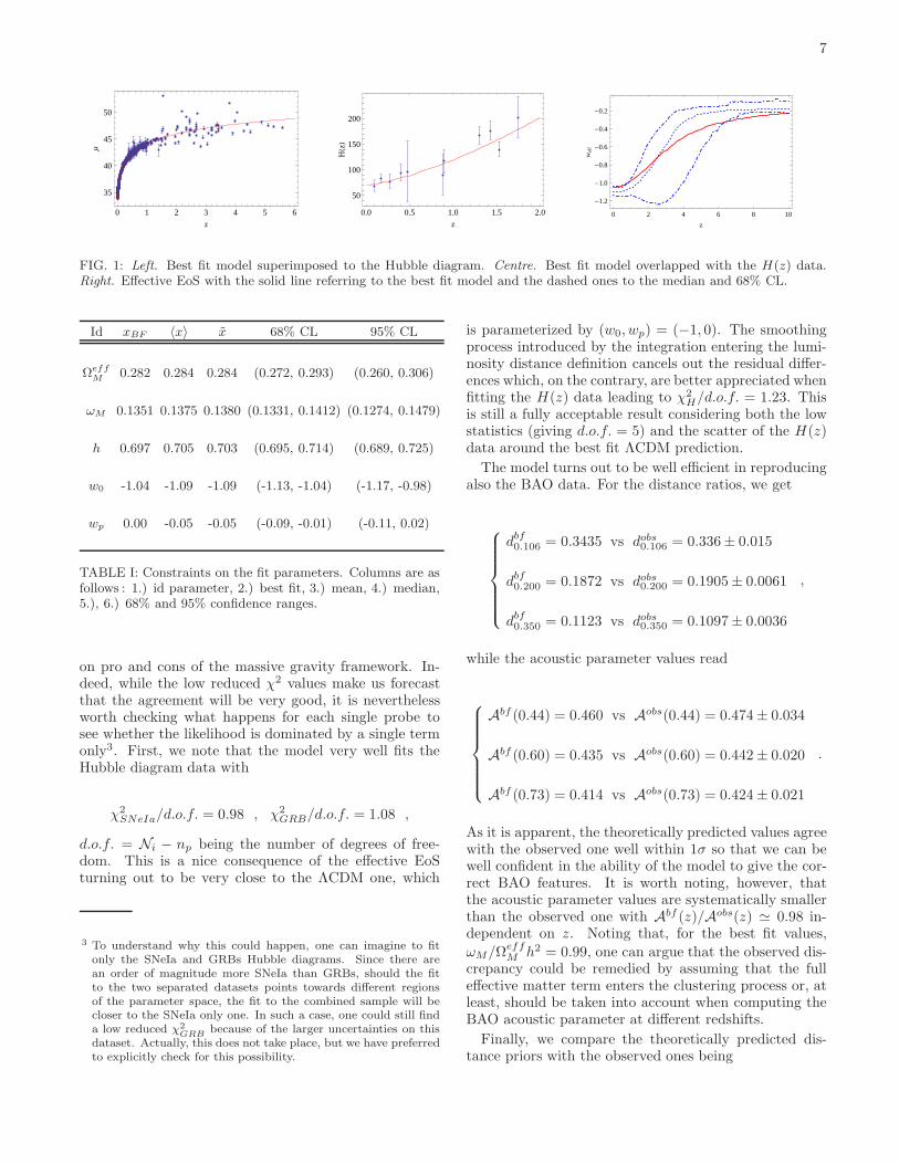
while its theoretical predictions for the Hubble diagramand the Hubble parameter are superimposed to the datain Fig. 1. Here, we also plot the effective dark energyEoS for the best fit model and the constraints from theMCMC analysis. To this end, for each z, we evaluateweff (z) for all the points in the chain and infer the me-dian value and 68% confidence ranges from the result-ing distribution. Note that the best fit weff (z) and themedian thus obtained are not equal because of the de-generacies in the model parameters space so that it isactually the median weff (z) the most reliable one in aBayesian framework since it takes explicitly into accountsuch degeneracies and marginalize over them.It is interesting to look in detail to how the best fit

model compares to the observed data to guess some hint

7

0 1 2 3 4 5 6

35

40

45

50

z

Μ

0.0 0.5 1.0 1.5 2.0

50

100

150

200

z

HHzL

0 2 4 6 8 10

-1.2

-1.0

-0.8

-0.6

-0.4

-0.2

z

wef

f

FIG. 1: Left. Best fit model superimposed to the Hubble diagram. Centre. Best fit model overlapped with the H(z) data.Right. Effective EoS with the solid line referring to the best fit model and the dashed ones to the median and 68% CL.

Id xBF 〈x〉 x 68% CL 95% CL

ΩeffM 0.282 0.284 0.284 (0.272, 0.293) (0.260, 0.306)

ωM 0.1351 0.1375 0.1380 (0.1331, 0.1412) (0.1274, 0.1479)

h 0.697 0.705 0.703 (0.695, 0.714) (0.689, 0.725)

w0 -1.04 -1.09 -1.09 (-1.13, -1.04) (-1.17, -0.98)

wp 0.00 -0.05 -0.05 (-0.09, -0.01) (-0.11, 0.02)

TABLE I: Constraints on the fit parameters. Columns are asfollows : 1.) id parameter, 2.) best fit, 3.) mean, 4.) median,5.), 6.) 68% and 95% confidence ranges.

on pro and cons of the massive gravity framework. In-deed, while the low reduced χ2 values make us forecastthat the agreement will be very good, it is neverthelessworth checking what happens for each single probe tosee whether the likelihood is dominated by a single termonly3. First, we note that the model very well fits theHubble diagram data with

χ2SNeIa/d.o.f. = 0.98 , χ2

GRB/d.o.f. = 1.08 ,

d.o.f. = Ni − np being the number of degrees of free-dom. This is a nice consequence of the effective EoSturning out to be very close to the ΛCDM one, which

3 To understand why this could happen, one can imagine to fitonly the SNeIa and GRBs Hubble diagrams. Since there arean order of magnitude more SNeIa than GRBs, should the fitto the two separated datasets points towards different regionsof the parameter space, the fit to the combined sample will becloser to the SNeIa only one. In such a case, one could still finda low reduced χ2

GRBbecause of the larger uncertainties on this

dataset. Actually, this does not take place, but we have preferredto explicitly check for this possibility.

is parameterized by (w0, wp) = (−1, 0). The smoothingprocess introduced by the integration entering the lumi-nosity distance definition cancels out the residual differ-ences which, on the contrary, are better appreciated whenfitting the H(z) data leading to χ2

H/d.o.f. = 1.23. Thisis still a fully acceptable result considering both the lowstatistics (giving d.o.f. = 5) and the scatter of the H(z)data around the best fit ΛCDM prediction.

The model turns out to be well efficient in reproducingalso the BAO data. For the distance ratios, we get

dbf0.106 = 0.3435 vs dobs0.106 = 0.336± 0.015

dbf0.200 = 0.1872 vs dobs0.200 = 0.1905± 0.0061

dbf0.350 = 0.1123 vs dobs0.350 = 0.1097± 0.0036

,

while the acoustic parameter values read

Abf (0.44) = 0.460 vs Aobs(0.44) = 0.474± 0.034

Abf (0.60) = 0.435 vs Aobs(0.60) = 0.442± 0.020

Abf (0.73) = 0.414 vs Aobs(0.73) = 0.424± 0.021

.

As it is apparent, the theoretically predicted values agreewith the observed one well within 1σ so that we can bewell confident in the ability of the model to give the cor-rect BAO features. It is worth noting, however, thatthe acoustic parameter values are systematically smallerthan the observed one with Abf (z)/Aobs(z) ≃ 0.98 in-dependent on z. Noting that, for the best fit values,

ωM/ΩeffM h2 = 0.99, one can argue that the observed dis-

crepancy could be remedied by assuming that the fulleffective matter term enters the clustering process or, atleast, should be taken into account when computing theBAO acoustic parameter at different redshifts.

Finally, we compare the theoretically predicted dis-tance priors with the observed ones being

8

ℓbfA = 302.023 vs ℓobsA = 302.09± 0.76

Rbf = 1.729 vs Robs = 1.725± 0.018

zbf⋆ = 1090.92 vs zobs⋆ = 1091.30± 0.91

so that the agreement is still excellent.The above results have been obtained contrasting the

model to the full observational probes we have describedin Sect. III which also include data from GRBs and theH(z) as inferred from galaxy ages. Although both thesedatasets are well fitted by the model, their use as cosmo-logical probes is quite recent so that one can not excludea priori that some undetected systematic is present andpotentially bias the constraints. As a consistency check,we have therefore repeated the above analysis removingboth GRBs and H(z) data from the fit. The medianvalue and 68% CL turn out to be :

ΩeffM = 0.282+0.012

−0.012 , ωM = 0.1316+0.0039−0.0061 ,

h = 0.685+0.012−0.008 , w0 = −1.06+0.05

−0.05 , wp = 0.06+0.03−0.02 .

These results are in good agreement with those in Table Iwith the 68% CL well overlapping for all the parametersbut wp. This latter quantity is the one with the largestshit since now positive rather than negative values arepreferred. Actually, for both fits, the results argue infavour of a very mild evolution of the effective EoS whichcan be easily smoothed out from the integration neededto get the luminosity distance. We therefore expect thatadding H(z) data erases this discrepancy. Indeed, fittingthis dataset too (but still excluding GRBs), we get :

ΩeffM = 0.284+0.008

−0.006 , ωM = 0.1399+0.0023−0.0061 ,

h = 0.710+0.005−0.010 , w0 = −1.07+0.03

−0.05 , wp = −0.07+0.03−0.03 ,

which are now in still better agreement with those in Ta-ble I with the wp confidence range moving towards neg-ative values. We also note that the median h value islarger and almost equal to the one from the fit to the fulldataset. This comes out as a consequence of the needfor the fit to align the present day H0 value to the trendfollowed by the z > 0 measurements. That this is thecase is also confirmed by the last test we do removingthe H(z) data, but adding the GRB ones. We now get :

ΩeffM = 0.284+0.011

−0.012 , ωM = 0.1347+0.0048−0.0055 ,

h = 0.695+0.010−0.005 , w0 = −1.07+0.04

−0.06 , wp = −0.01+0.02−0.03 .

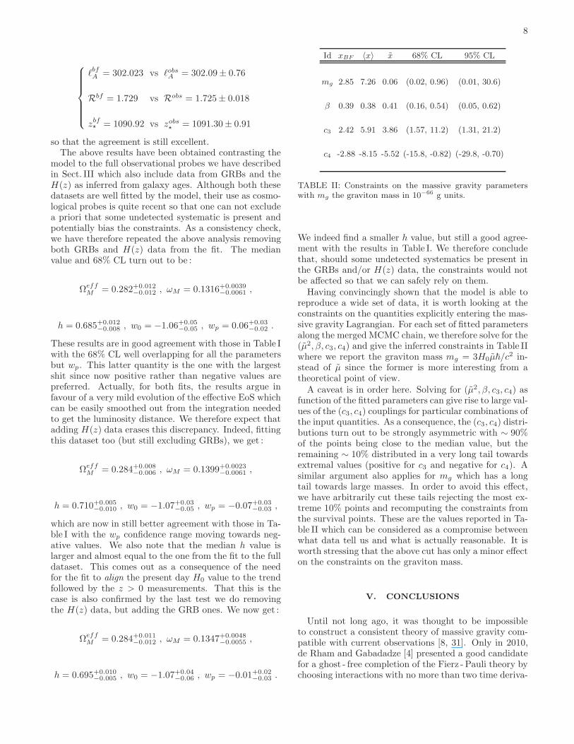
Id xBF 〈x〉 x 68% CL 95% CL

mg 2.85 7.26 0.06 (0.02, 0.96) (0.01, 30.6)

β 0.39 0.38 0.41 (0.16, 0.54) (0.05, 0.62)

c3 2.42 5.91 3.86 (1.57, 11.2) (1.31, 21.2)

c4 -2.88 -8.15 -5.52 (-15.8, -0.82) (-29.8, -0.70)

TABLE II: Constraints on the massive gravity parameterswith mg the graviton mass in 10−66 g units.

We indeed find a smaller h value, but still a good agree-ment with the results in Table I. We therefore concludethat, should some undetected systematics be present inthe GRBs and/or H(z) data, the constraints would notbe affected so that we can safely rely on them.Having convincingly shown that the model is able to

reproduce a wide set of data, it is worth looking at theconstraints on the quantities explicitly entering the mas-sive gravity Lagrangian. For each set of fitted parametersalong the merged MCMC chain, we therefore solve for the(µ2, β, c3, c4) and give the inferred constraints in Table IIwhere we report the graviton mass mg = 3H0µ~/c

2 in-stead of µ since the former is more interesting from atheoretical point of view.A caveat is in order here. Solving for (µ2, β, c3, c4) as

function of the fitted parameters can give rise to large val-ues of the (c3, c4) couplings for particular combinations ofthe input quantities. As a consequence, the (c3, c4) distri-butions turn out to be strongly asymmetric with ∼ 90%of the points being close to the median value, but theremaining ∼ 10% distributed in a very long tail towardsextremal values (positive for c3 and negative for c4). Asimilar argument also applies for mg which has a longtail towards large masses. In order to avoid this effect,we have arbitrarily cut these tails rejecting the most ex-treme 10% points and recomputing the constraints fromthe survival points. These are the values reported in Ta-ble II which can be considered as a compromise betweenwhat data tell us and what is actually reasonable. It isworth stressing that the above cut has only a minor effecton the constraints on the graviton mass.

V. CONCLUSIONS

Until not long ago, it was thought to be impossibleto construct a consistent theory of massive gravity com-patible with current observations [8, 31]. Only in 2010,de Rham and Gabadadze [4] presented a good candidatefor a ghost - free completion of the Fierz - Pauli theory bychoosing interactions with no more than two time deriva-

9

tives of the scalar degrees of freedom [4]. The cosmologi-cal sector of this theory have been recently worked out in[5, 13] thus setting the necessary framework to comparethe model predictions with the observed universe. Wehave then been able to constrain the model parametersusing a large dataset comprising the SNeIa+GRB Hub-ble diagram, H(z) measurements from cosmic chronome-ters, BAOs data and the CMBR distance priors. It turnsout that the model is in very good agreement with thedata thus giving an observationally motivated support tomassive gravity as a theoretically appealing alternativethe the troublesome ΛCDM scenario.Lacking up to now a clear physical interpretation of

the (c3, c4) couplings entering the modified gravity La-grangian, one can only indirectly check which are theconditions they have to fulfil in order the theory be con-sistent. To this end, we stress that our constraints areconsistent with the conditions c3 + c4 = 0 and c4 6= −1,but the case c3 + c4 > 0 is still allowed. In both cases,the constrained parameter space refers to models whichhave the right properties to recover GR in the low energylimit as demonstrated by [34] through the study of spher-ically symmetric solutions. We therefore end up with amassive gravity theory able to reproduce the cosmolog-ical data without altering the success of the standardGeneral Relativity on the Solar System scales.As a further relevant result, the comparison of the the-

ory with the cosmological data has allowed us to set alimit on the graviton mass. Although an explicit deriva-tion is needed, we can assume that, in the low energylimit, the gravitational potential will be boosted by a

Yukawa - like correction modulated by the length scaleλg ∝ 1/mg. One can then compare our results withthe upper limit mg < 7.68× 10−55 g from the dynamicsin the Solar System [32] and the more stringent limit,mg < 10−59 g, derived by requiring the derived dynam-ical properties of a galactic disk to be consistent withobservations [33]. Our 95% upper limit is six orders ofmagnitude smaller than the latter one. We can thereforeconclude that the agreement with the cosmological dataleads to a massive gravity theory which has no impacton the dynamics of sytems in the low energy regime thusavoiding any difficulty in matching different scales.

Finally, since covariant massive gravity seems to be aconsistent modification of GR, it would be interesting andworthwhile to further explore it. In particular, investiga-tion should be improved by analyzing perturbed solutionsand full prediction of cosmological perturbations.

Acknowledgements

LP would like to thank R. Maartens for thoughtfuladvice. LP and NR would like to thank G. Vilasi forcontinuous encouraging and supporting. VFC is sup-ported by Agenzia Spaziale Italiana (ASI) through con-tract Euclid - IC (I/031/10/0). NR and LP acknowl-edge partial support by a INFN/MICINN collaboration,Agenzia Spaziale Italiana (ASI) and the Italian Minis-tero Istruzione Universita e Ricerca (MIUR) through thePRIN2008 project.

[1] A.G. Riess et al., AJ, 116, 1009, 1998; S. Perlmutter etal., ApJ, 517, 565, 1999;

[2] D.N. Spergel et al., ApJS, 148, 175, 2003; S. Cole et al.,MNRAS, 362, 505, 2005; M. Kowalski et al., ApJ, 686,749, 2008; D.N. Spergel et al., ApJS, 170, 377, 2007

[3] M. Fierz, W. Pauli, Proc. Roy. Soc. Lond. A 173, 211,1939

[4] C. de Rham, G. Gabadadze, Phys. Rev. D, 82, 044020,2010

[5] A.H. Chamseddine, M.S. Volkov, Phys. Lett. B, 704, 652,2011

[6] D.G. Boulware, S. Deser, Phys. Rev. D, 6, 3368, 1972[7] N. Arkani -Hamed, H. Georgi, M.D. Schwartz, Annals

Phys., 305, 96, 2005[8] P. Creminelli, A. Nicolis, M. Papucci, E. Trincherini,

JHEP, 0509, 003, 2005[9] C. de Rham, G. Gabadadze, A.J. Tolley, Phys. Rev.

Lett., 106, 2311101, 2011[10] S.F. Hassan, R.A. Rosen, preprint arXiv :1106.3344, 2011[11] T.M. Nieuwenhuizen, Phys. Rev. D, 84, 024038, 2011[12] E. Komatsu, K.M. Smith, J. Dunkley, C.L. Bennett, B.

Gold, et al., ApJS, 192, 18, 2011[13] M.S. Volkov, JHEP, 1201, 035 (2012)[14] R. Amanullah, C. Lidman, C., D. Rubin, G. Aldering, P.

Astier, et al. ApJ, 716, 712, 2010[15] V.F. Cardone, M. Perillo, S. Capozziello, MNRAS, 417,

1672, 2011[16] L. Xiao, B.E. Schaefer, ApJ, 731, 103, 2011[17] R. Jimenez, A. Loeb, ApJ, 573, 37, 2002[18] D. Stern, R. Jimenez, L. Verde, S.A. Stanford, M.

Kamionkowski, ApJS, 188, 280, 2010[19] D. Stern, R. Jimenez, L. Verde, M. Kamionkowski, S.A.

Stanford, JCAP, 02, 008, 2010[20] D.J. Eisenstein, W. Hu, M. Tegmark, ApJ, 504, 57, 1998;

A. Cooray, W. Hu, D. Huterer, M. Joffre, ApJ, 557, L7,2001; C.A. Blake, K. Glazebrook, ApJ, 594, 665, 2003;W. Hu, Z. Haiman, Phys. Rev. D, 68, 063004, 2003

[21] D.J. Eisenstein, I. Zehavi, D.W. Hogg, R. Scoccimarro,M.R. Blanton, et al., ApJ, 633, 560, 2005

[22] S. Cole, W.J. Percival, J.A. Peacock, P. Norberg, C.M.Baugh, MNRAS, 362, 505, 2005; G. Hutsi, A&A, 449,891, 2006; A.G. Sanchez, M. Crocce, A. Cabre, C.M.Baugh, E. Gaztanaga, MNRAS, 400, 1643, 2009; E.A.Kazin, M.R. Blanton, R. Scoccimarro, C.K. McBride,A.A. Berlind, et al., ApJ, 710, 1444, 2010; C. Blake, A.Collister, S. Bridle, O. Lahav, MNRAS, 374, 1527, 2007;N. Padmanabhan, D.J. Schlegel, U. Seljak, A. Makarov,N.A. Bahcall, et al., MNRAS, 378, 852, 2007; M. Crocce,E. Gaztanaga, A. Cabre, A. Carnero, E. Sanchez, MN-RAS, 417, 2577, 2011

[23] F. Beutler, C. Blake, M. Colless, D.H. Jones, L. Staveley -Smith, et al., MNRAS, 416, 3017, 2011

10

[24] W.J. Percival, B.A. Reid, D.J. Eisenstein, N.A. Bahcall,T. Budavari, et al., MNRAS, 401, 2148, 2010

[25] C. Blake, E.A. Kazin, F. Beutler, T.M. Davis, D. Parkin-son, et al., MNRAS, 418, 1707, 2011

[26] J.R. Bond, G. Efstathiou, M. Tegmark, MNRAS, 291,L33, 1997; L. Page, M.R. Nolta, C., Barnes, C.L. Ben-nett, M. Halpern, et al. ApJS, 148, 233, 2003

[27] W. Hu, N. Sugiyama, ApJ, 471, 542, 1996[28] A. Riess, L. Macri, S. Casertano, M. Sosey, H. Lampeitl,

et al., ApJ, 699, 539, 2009[29] K. Koyama, G. Niz, G. Tasinato, Phys. Rev. D, 84,

064033, 2011[30] A. Gelman, D.B. Rubin, Stat. Sci., 7, 457, 1992[31] C. Deffayet and J. W. Rombouts, Phys. Rev. D 72,

044003 (2005)[32] C. Talmadge, J.P. Berthias, R.W. Hellings, E.M. Stan-

dish, Phys. Rev. Lett., 61, 1988[33] M.E.S. Alves, O.D. Miranda, J.C.N. de Araujo, Gen. Rel.

Grav., 39, 777, 2007[34] K. Koyama, G. Niz and G. Tasinato, Phys. Rev. D 84,

064033, 2011