Constraining scalar-tensor quintessence by cosmic clocks

arX

iv:0

706.

2615

v1 [

astr

o-ph

] 18

Jun

200

7Astronomy & Astrophysicsmanuscript no. lookbackjaafinal c© ESO 2008February 1, 2008

Constraining scalar-tensor quintessence by cosmic clocksS. Capozziello1,2, P.K.S. Dunsby3,E. Piedipalumbo1,2, C. Rubano1,2

1 Dipartimento di Scienze Fisiche, Universita di Napoli “Federico II”2 Istituto Nazionale di Fisica Nucleare, Sez. Napoli, Via Cinthia, Compl. Univ. Monte S. Angelo, 80126 Naples, Italy3 Department of Mathematics and Applied Mathematics, University of Cape Town and

South African Astronomical Observatory, Observatory CapeTown, South Africa.

Received/ Accepted

ABSTRACT

Aims. To study scalar tensor theories of gravity with power law scalar field potentials as cosmological models for accelerating universe,using cosmic clocks.Methods. Scalar-tensor quintessence models can be constrained by identifying suitable cosmic clocks which allow to select confidenceregions for cosmological parameters. In particular, we constrain the characterizing parameters of non-minimally coupled scalar-tensorcosmological models which admit exact solutions of the Einstein field equations. Lookback time to galaxy clusters at lowintermediate,and high redshifts is considered. The high redshift time-scale problem is also discussed in order to select other cosmicclocks such asquasars.Results. The presented models seem to work in all the regimes considered: the main feature of this approach is the fact that cosmicclocks are completely independent of each other, so that, inprinciple, it is possible to avoid biases due to primary, secondary and soon indicators in the cosmic distance ladder. In fact, we haveused different methods to test the models at low, intermediate and highredshift by different indicators: this seems to confirm independently the proposed dark energy models.

Key words. cosmology: theory - cosmology: quintessence -Noether symmetries-Scalar tensor theories

1. Introduction

An increasing harvest of observational data seems indicatethat≃ 70% of the present day energy density of the universeis dominated by a mysterious ”dark energy” component, de-scribed in the simplest way using the well known cosmolog-ical constantΛ (Perlmutter et al., 1997, Perlmutter et al., 1999,Riess et al., 1998, Riess, 2000) and explains the accelerated ex-pansion of the observed Universe, firstly deduced by luminositydistance measurements. However, even though the presence of adark energy component is appealing in order to fit observationalresults with theoretical predictions, its fundamental nature stillremains a completely open question.

Although several models describing the dark energy compo-nent have been proposed in the past few years, one of the firstphysical realizations of quintessence was a cosmological scalarfield, which dynamically induces a repulsive gravitationalforce,causing an accelerated expansion of the Universe.

The existence of such a large proportion of dark energy inthe universe presents a large number of theoretical problems.Firstly, why do we observe the universe at exactly the time inits history when the vacuum energy dominates over the matter(this is known as thecosmic coincidenceproblem). The secondissue, which can be thought of as afine tuning problem, arisesfrom the fact that if the vacuum energy is constant, like in thepure cosmological constant scenario, then at the beginningofthe radiation era the energy density of the scalar field shouldhave been vanishingly small with respect to the radiation andmatter component. This poses the problem, that in order to ex-plain the inflationary behaviour of the early universe and the late

Send offprint requests to: S. Capozziello, [email protected]

time dark energy dominated regime, the vacuum energy shouldevolve and cannot simply beconstant.

A recent work has demonstrated that the fine-tuning problemcan be alleviated by selecting a subclass of quintessence models,which admit atracking behaviour(Steinhardt et al, 1999), andin fact, to a large extent, the study of scalar field quintessencecosmology is often limited to such a subset of solutions. Inscalar field quintessence, the existence condition for a trackersolution provides a sort of selection rule for the potentialV(φ)(see (Rubano et al., 2004) for a critical treatment of this ques-tion), which should somehow arise from a high energy physicsmechanism (the so calledmodel building problem). Also adopt-ing a phenomenological point of view, where the functionalform of the potentialV(φ) can be determined from observationalcosmological functions, for example the luminosity distance,we still cannot avoid a number of problems. For example, anattempt to reconstruct the potential from observational data(and also fitting the existing data with a linear equation of state)shows that a violation of the weak energy condition (WEC) isnot completely excluded (Caldwell et al., 2003), and this wouldimply a superquintessence regime, during which wφ < −1(phantom regime). However it turns out that, assuming a darkenergy component with an arbitrary scalar field Lagrangian,the transition from regimes withwφ ≥ −1 to those withwφ < −1 (i.e. crossing the so calledphantom divide) couldbe physically impossible since they are either described byadiscrete set of trajectories in the phase space or are unstable(Hu, 2005, Vikman, 2005). These shortcomings have beenrecently overcome by considering theunified phantom cosmol-ogy (Nojiri & Odintsov, 2005) which, by taking into account ageneralised scalar field kinetic sector, allows to achieve modelswith natural transitions between inflation, dark matter, and dark

http://arXiv.org/abs/0706.2615v1

2 S. Capozziello & al.: Constraining scalar-tensor quintessence by cosmic clocks

energy regimes. Moreover, in recent works, a dark energy com-ponent has been modeled also in the framework of scalar tensortheories of gravity, also called extended quintessence (see forinstance Boisseau et al., 2000, Fujii, 2000, Perrotta et al., 2000,Dvali et al., 2000, Chiba, 1999, Amendola, 1999,Uzan, 1998, Capozziello, 2002, Capozziello et al., 2003,Nojiri & Odintsov, 2003, Vollick, 2003, Meng & Wang, 2003,Allemandi et al., 2004). Actually it turns out that they arecompatible with apeculiar equation of statew ≤ −1, andprovide a possible link to the issues of non-Newtonian gravity(Fujii, 2000). In such theoretical background the acceleratedexpansion of the universe results in an observational effect ofa non-standard gravitational action. In extended quintessencecosmologies (EQ) the scalar field is coupled to the Ricci scalar,R, in the Lagragian density of the theory: the standard term16πG∗ R is replaced by 16πF(φ) R, whereF(φ) is a functionof the scalar field, andG∗ is the bare gravitational constant,generally different to the Newtonian constantGN measured inCavendish-type experiments (Boisseau et al., 2000). Of course,the coupling is not arbitrary, but it is subjected to severalcon-straints, mainly arising from the time variation of the constantsof nature (Riazuelo & Uzan, 2002). In EQ models, a scalar fieldhas indeed a double role: it determines at any time the effectivegravitational constant and contributes to the dark energy density,allowing some different features with respect to the minimallycoupled case (Riazuelo & Uzan, 2002). Actually, while in theframework of the minimally coupled theory we have to deal witha fully relativistic component, which becomes homogeneousonscales smaller than the horizon, so that standard quintessencecannot cluster on such scales, in the context of nonminimallycoupled quintessence theories the situation changes, and thescalar field density perturbations behave like the perturbationsof the dominant component at any time, demonstrating in the socalledgravitational dragging(Perrotta et al., 2000).

In this work, we focus our attention on the effect that dark en-ergy has on the background evolution (through thet(z) relation)in the framework of some scalar tensor quintessence models,forwhich exact solutions of the field equations are known. In par-ticular we show that an accurate determination of the age of theuniverse together with new age determinations of cosmic clockscan be used to produce new strict constraints on these dark en-ergy models, by constructing the time-redshift (t − z) relation,and comparing the theoretical predictions with the observationaldata.

Although discrepancies between age determinations havelong plagued cosmology, the situation has changed dramaticallyin recent years: type Ia supernova measurements, the acousticpeaks in the CMB anisotropies (Spergel et al., 2003), and so on,are all consistent with an aget0 ≃ 14±1Gyr. Recently Krauss &Chaboyer (Krauss & Chaboyer, 2003) have provided constraintson the equation of state of the dark energy by using new globularcluster age estimates.

Furthermore, Jimenez & al. proposed a non parametricmeasurements of the time dependence ofw(z), based on therelative ages of stellar populations (Jimenez & Loeb, 2002,Jimenez et al., 2003). It is therefore rather timely to investigatethe implications of new age measurements within in the frame-work of quintessence cosmology.

It turns out that such (t − z) relations are strongly varyingfunctions of the equation of statew(z), and could also be veryuseful for breaking the degeneracies that arise in other observa-tional tests.

As a first step toward this goal, we study the cosmo-logical implications arising from the existence of the quasar

APM 08279+5255 and three extremely red radio galaxies atz = 1.175 (3C65),z = 1.55 (53W091) andz = 1.43(53W069) with a minimal stellar age of 4.0 Gyr, 3.0 Gyrand 4.0 Gyr, respectively, extending the analysis performedin (Lima & Alcaniz, 2000, Alcanitz et al., 2003) to a scalar-tensor field quintessential model (Capozziello & de Ritis, 1994,Demianski et al., 2006, Capozziello et al, 1996).

As a further step, we also consider thelookback timeto distant objects, which is observationally estimated as thedifference between the present day age of the universe andthe age of a given object at redshiftz, already used in(Capozziello et al., 2004) to constrain dark energy models.Suchan estimate is possible if the object is a galaxy observed in morethan one photometric band, since its color is determined by itsage as a consequence of stellar evolution.

It is thus possible to get an estimate of the galaxy age bymeasuring its magnitude in different bands and then using stellarevolutionary codes. It is worth noting, however, that the estimateof the age of a single galaxy may be affected by systematic errorswhich are difficult to control.

It turns out that this problem can be overcome by consid-ering a sample of galaxies belonging to the same cluster. Inthis way, by averaging the age estimates of all the galaxies,one obtains an estimate of the cluster age and thereby reduc-ing the systematic errors. Such a method was first proposed byDalal & al. (Dalal et al., 2001) and then used by Ferreras & al.(Ferreras et al., 2003) to test a class of models where a scalarfield is coupled to the matter term, giving rise to a particularquintessence scheme. We improve here this analysis by usinga different cluster sample (Andreon et al, 2004, Andreon, 2003)and testing a scalar tensor quintessence model. Moreover, weadd a further constraint to better test the dark energy models andassume that the age of the universe for each model is in agree-ment with recent estimates. Note that this is not equivalentto thelookback time method as we will discuss below.

The layout of the paper is as follows. In Sect. 2, we brieflypresent the class of cosmological models which we are going toconsider, defining also the main quantities which we need forthelookback time test. Sects. 3 and 4 are devoted to the discussionof cosmic clocks at low, intermediate and high redshifts whoseobservational data are used to test the theoretical backgroundmodel. Finally we summarize and draw conclusions in Sect. V.The lookback time method is outlined in the Appendix A, refer-ring to (Capozziello et al., 2004) for a detailed exposition.

2. The model

The action for a scalar-tensor theory, where a genericquintessence scalar field is non-minimally coupled with grav-ity, and a minimal coupling between matter and the quintessencefield is assumed, is:

A =∫

T

√−g

(F(φ)R+

12

gµνφ,µφ,ν − V(φ) + Lm

), (1)

whereF(φ), and V(φ) are two generic functions, representingthe coupling with geometry and the potential respectively,R

is the curvature scalar,12

gµνφ,µφ,ν is the kinetic energy of the

quintessence fieldφ andLm describes the standard matter con-tent. In units 8πG = ~ = c = 1 and signature (+, -, -, -), werecover the standard gravity forF = −1/2, while the effective

gravitational coupling isGe f f = −1

2F. Chosing a spatially flat

S. Capozziello & al.: Constraining scalar-tensor quintessence by cosmic clocks 3

Friedman-Robertson-Walker metric in Eq. (1), it is possible toobtain thepointlikeLagrangian

L = 6Faa2 + 6F′φa2a+ a3pφ − D , (2)

wherea is the expansion parameter andD is the initial dust-matter density. Here prime denotes derivative with respectto φand dot the derivative with respect to cosmic time. The dynami-cal equations, derived from Eq. (2), are

H2 = − 12F

(ρφ3+ρm

3

), (3)

2H + 3H2 =1

2Fpφ , (4)

where the pressure and the energy density of theφ-field are givenby

pφ =12φ2 − V(φ) − 2(F + 2HF) , (5)

ρφ =12φ2 + V(φ) + 6HF , (6)

andρm is the standard matter-energy density. Considering Eq.(2), the variation with respect toφ gives the Klein-Gordon equa-tion

φ + 3Hφ + 12H2F′ + 6HF′ + V′ = 0 . (7)

2.0.1. The case of power law potentials

Recently it has been shown that it is possible to determine thestructure of a scalar tensor theory, without choosing any specifictheory a priori, but instead reconstructing the scalar fieldpoten-tial and the functional form of the scalar-gravity couplingfromtwo observable cosmological functions: the luminosity distanceand the linear density perturbation in the dustlike matter com-ponent as functions of redshift. Actually the most part of workswhere scalar-tensor theories were considered as a model foravariableΛ-term followed either areconstructionpoint of view,either a traditional approach, with some special choices ofthescalar field potential and the coupling. However it is possiblealso athird road to determine the structure of a scalar tensortheory, requesting some general and physically based properties,from which it is possible to select the functional form of thecou-pling and the potential. An instance of such a procedure has beenproposed in (Demianski et al., 1991, Capozziello et al, 1996): itturns out that requiring the existence of a Noether symmetryforthe action in Eq. (1), it is possible not only to select several ana-lytical forms both forF(φ) andV(φ), but also obtain exact solu-tions for the dynamical system (3,4,7). In this section we analyzea wide class of theories derived from such a Noether symmetryapproach, which show power law couplings and potentials, andadmit atracker behaviour. Let us summarize the basic results,referring to (Demianski et al., 2006, Demianski et al., 2007) fora detailed exposition of the method. It turns out that the Noethersymmetry exists only when

V = V0(F(φ))p(s) , (8)

whereV0 is a constant and

p(s) =3(s+ 1)2s+ 3

, (9)

where s labels the class of such Lagrangians which admit aNoether symmetry. A possible choice ofF(φ) is

F = ξ(s)(φ + φi)2 , (10)

where

ξ(s) =(2s+ 3)2

48(s+ 1)(s+ 2), (11)

and φi is an integration constant. The general solution corre-sponding to such a potential and coupling is:

a(t) = A(s)

(B(s)t

3s+3 +

DΣ0

) s+1s

t2s2+6s+3

s(s+3) , (12)

φ(t) = C(s)

(− V0

γ(s)B(s)t

3s+3 +

DΣ0

)− 2s+32s

t−(2s+3)2

2s(s+3) , (13)

whereA(s), B(s), C(s), γ(s) andχ(s) are given by

A(s) = (χ(s))s+1s

((s+ 3)Σ0

3γ(s)

) s+2s+3

, (14)

B(s) =

((s+ 3)Σ0

3γ(s)

)− 3(s+3) (s+ 3)2

s+ 6, (15)

C(s) = (χ(s))−(2s+3)

2s

((s+ 3)Σ0

3γ(s)

)− (3+2s)2(s+3)

, (16)

and

γ(s) =2s+ 3

12(s+ 1)(s+ 2), (17)

χ(s) = − 2s2s+ 3

, (18)

whereD is the matter density constant,Σ0 is an integration con-stant resulting from the Noether symmetry, andV0 is the constantwhich determines the scale of the potential. Even if these con-stants are not directly measurable, they can be rewritten intermsof cosmological observables likeH0,Ωm etc, as in the following:

D =

(

1A(s)

) ss+1

− B(s)

Σ0 , (19)

Σ0 =

(3−

5s+6s2+4s+3 (s+ 3)−

3s2+7s+3s2+4s+3 (s+ 6) ×

×

((H0 − 2)s2 + 3(H0 − 2)s− 3

)γ(s)

s2−s−3s2+4s+3

(s+ 1)χ(s)

(s+1)(s+3)s2−s−3

. (20)

Here we are following the procedure used in(Demianski et al., 2006), taking the age of the universe,t0,as a unit of time. Because of our choice of time unit, the ex-pansion rateH(t) is dimensionless, so that our Hubble constantis not (numerically) the same as theH0 that appears in thestandard FRW model and measured in kms−1Mpc−1. Settinga0 = a(t0) = 1 andH0 = H(t0), we are able to writeΣ0 andD asfunctions ofs andH0. Since the effective gravitational couplingis Ge f f = − 1

2F , it turns out that in order to recover an attractivegravity we gets ∈ (−2 , −1). Restricting furthermore the valuesof s to the ranges ∈ (− 3

2 , −1) the potentialV(φ) is an inversepower-law,φ−2|p(s)|. In this framework, we obtain naturally aneffective cosmological constant:

Λe f f = Ge f fρφ, (21)


where limt→∞ Λe f f = Λ∞ , 0. It is then possible to associate aneffective density parameterto theΛ term, via the usual relation

ΩΛe f f ≡Λe f f

3H2. (22)

Eqs. (12) and (13) are all that is needed to perform thet − zanalysis. It is worth noting that, since the lookback time - red-shift (t − z) relation does not depend on the actual value oft0,it furnishes an independent cosmological test through age mea-surements, especially when it is applied to old objects at highredshifts. For varyingw, as in the case of our model, the look-back time can be rewritten in a more general form by considering

H0t0 =∫ 1

0

H0daaH(a)

,

and then writing

tL(z) = tH

∫ a

0

H0daaH(a)

,

wherea = 1/(1+ z) andtH = 1H0

is theHubble time.

2.0.2. The case of quartic potentials

As it is clear from Eq.(12) and Eq.(13) for a generic value ofsboth the scale factora(t) and the scalar fieldφ(t) have a powerlaw dependence on time. It is also clear that there are someadditional particular values ofs, namelys = 0 and s = −3which should be treated independently. Actuallys = 0 re-duces to the minimally coupled case (see Demianski et al., 2005)while s = −3 corresponds to the induced gravity with a quar-tic potentials: namely,F = 3

32φ2, andV(φ) = λφ4 . This case

is particularly relevant since it allows one to recover the self-interaction potential term of several finite temperature field the-ories. In fact, the quartic form of potential is required in or-der to implement the symmetry restoration in several GrandUnified Theories. Consequently, we limit our analysis to thismodel, showing that it naturally provides an accelerated ex-pansion of the universe and other interesting features of darkenergy models. It worth to note that since thespecialderiva-tion of our model, we can focus the analysis on quantitiesconcerning, mostly, the background evolution of the universe,without recurring to any observable related to the evolution ofperturbations. The following analysis can be easily extendedto more general classes of non-minimally coupled theories,where exact solutions can be achieved by Noether symmetries(Capozziello et al, 1996, Capozziello & de Ritis, 1993), but, forthe sake of simplicity, we restrict only to the above relevant case.The general solution is

a(t) = aie−α1t

3[(−1+ eα1 t) + α2 t + α3

] 23 , (23)

φ = φi

√e−α1t

(−1+eα1 t)+α2 t+α3, (24)

whereα1 = 4√λ, andai , α2 α3 andφi are integration constants,

related to the initial matter density,D, by the relationα1α2 = D,which implies that they cannot be null. The caseλ = 0 has to betreated separately.

It turns out thatα3, φi and ai have an immediate physicalinterpretation:ai is connected to the value of the scale factor att = t0 = 1, whileα3 set the valuea(0). We can

safely seta(0) = 0, so thatα3 = 0. Actually this is not strictlycorrect, as our model does not extend up to the initial singularity.

However, this position introduces a shift in the time scale whichis small with respect to that of the radiation dominated era.Thisalters by a negligible amount the value oft0, while, moreover, itis left undetermined in our parametrisation.

Since F(φ) ∝ φ2, andGe f f(φ) ∝ − 1F(φ) , we note that a way

of recovering attractive gravity is to choseφi as a pure imaginarynumber. Without compromising the general nature of the prob-lem, we can setφi = ı, so that our field in Eq. (24) becomes apurely imaginary field, giving rise to an apparent inconsistencywith the choice in the Lagrangian (2). Actually, the genericin-finitesimal generator of the Noether symmetry is

X = α∂

∂a+ β

∂

∂φ+ α

∂

∂a+ β

∂

∂φ, (25)

whereα andβ are both functions ofa andφ, and:

α ≡ ∂α

∂aa+

∂α

∂φφ ; β ≡ ∂β

∂aa+

∂β

∂φφ. (26)

Demanding the existence of Noether symmetryLXL = 0, we getthe following equations,

α + 2a∂α

∂a+ a2∂β

∂aF′

F+ aβ

F′

F= 0 (27)

(2α + a

∂α

∂a+ a

∂β

∂φ

)F′ + aF′′β + 2F

∂α

∂φ+

a2

6∂β

∂a= 0 (28)

3α + 12F′(φ)∂α

∂φ+ 2a

∂β

∂φ= 0 (29)

V′

V= p(s)

F′

F(30)

It turns out that these equations are preserved if we adopt themore common signature (−,+,+,+) in the metric tensor and flipthe sign of the kinetic term. This imply that the generic infinites-imal generator of the Noether symmetry is preserved, and henceprovidesphantomsolutions of the field equations. Therefore, asfar as thequaestioof settingφi = ı concerns, it turns out that thescalar field can be physically interpreted as aphantomsolutionof the field equations adopting the signature (−,+,+,+), evenif it is mathematically represented as a pure imaginary field. Itworth noting that such phantom solutions in scalar tensor gravitydo not produce any violation in energy conditions, sinceρφ, ρφ+pφ andρφ+3pφ are strictly positive in the minimally coupled case(see Ellis & Madsen, 1991 and references therein for a discus-sion). Furthermore, complex scalar fields (in particular purelyimaginary ones) have been widely considered in classical andquantum cosmology with minimal and non-minimal couplingsgiving rise to interesting boundary conditions for inflationary be-haviors Amendola et al., 1994, Kamenshchik et al., 1995.

Finally, assumingH(1) = H0, we get

a(t) = aie−α1t3

(eα1t − (3H0(eα1−1)−α1(eα1+1))t

3H0+α1−2 − 1)2/3

(31)

φ2(t) = − eα1t

eα1t− (3H0(eα1−1)−α1(eα1+1))t3H0+α1−2 −1

, (32)

where

ai = eα13

(3H0 + α1 − 2

2+ 2eα1(α1 − 1)

)2/3

. (33)


We have to note thatδ ≡Ge f f

Ge f f=

3H0 − α1

2, and stillα1 ≃

3H0, as we shall see in the next section, this expression is verysmall, as indicated by observations. This fact means that allphysical processes implying the effective gravitational constantare not dramatically affected in the framework of our model.

2.1. Some remarks

Before starting the detailed description of our method to use theage measurements of a given cosmic clock to get cosmologicalconstraints, it worth considering some caveats connected withour model. We concentrate in particular on the Newtonian limitand Post Parametrized Newtonian (PPN) parameters constraintsof this theory, and discuss some advantages related to the use ofthe t(z) relation, with respect to the magnitude - redshift one, toconstrain the cosmological parameters.

2.1.1. Newtonian limit and Post Parametrized Newtonian(PPN) behaviour

Recently the cosmological relevance of extended gravity theo-ries, as scalar tensor or high order theories, has been widelyexplored. However, in the weaklimit approximation, all theseclasses of theories should be expected to reproduce the Einsteingeneral relativity which, in any case, is experimentally testedonly in this limit. This fact is matter of debate since severalrelativistic theories do not reproduce Einstein results attheNewtonian approximation but, in some sense, generalize them,giving rise, for example, to Yukawa like corrections to theNewtonian potential which could have interesting physicalcon-sequences. In this section we want to discuss the Newtonian limitof our model, and study the Post Parametrized Newtonian (PPN)behaviour. In order to recover the Newtonian limit, the metrictensor has to be decomposed as

gµν = ηµν + hµν , (34)

whereηµν is the Minkoskwi metric andhµν is a small correctionto it. In the same way, we define the scalar fieldψ as a perturba-tion, of the same order of the components ofhµν, of the originalfield φ, that is

φ = ϕ0 + ψ , (35)

whereϕ0 is a constant of order unit. It is clear that forϕ0 = 1andψ = 0 Einstein general relativity is recovered. To write in anappropriate form the Einstein tensorGµν, we define the auxiliaryfields

hµν ≡ hµν −12ηµνh , (36)

and

σα ≡ hαβ,γηβγ . (37)

Given these definitions it turns out that the weak field limit ofthe power-law potential gives (see Demianski et al., 2007)

h00 ≃[ϕ2

01− 16ξ(s)

2ξ(s)(1− 12ξ(s))

]Mr

−

M ϕ20

1− 12ξ(s)V0(p(s) − 4)(p(s) − 1)

1− 2ξ(s)

r (38)

− 4π

V0ϕ

2+p(s)0

ξ(s)+

2ϕ40

2(p(s) − 1)V0(p(s) − 4)(p(s) − 1)

1− 2ξ(s)

r2

hi j ≃ δi j

[ϕ2

01− 8ξ(s)

2ξ(s)(1− 12ξ(s))

]Mr

+

M ϕ2

0

1− 12ξ(s)V0(p(s) − 4)(p(s) − 1)

1− 2ξ(s)

r (39)

+ 4π

V0ϕ

2+p(s)0

ξ(s)−

2ϕ40

2(p(s) − 1)V0(p(s) − 4)(p(s) − 1)

1− 2ξ(s)

r2

,

where only linear terms inV0 are given and we omitted the con-stant terms.

In the case of the quartic potential case, instead we obtain:

h00 ≃12

ϕ20(1− 16ξ)

ξ(1− 12ξ)

Mr−

4πλϕ6

0

ξ

r2 − Θ , (40)

hil ≃ δil

12

ϕ20(1− 8ξ)

ξ(1− 12ξ)

Mr+

4πλϕ6

0

ξ

r2 + Θ

, (41)

ψ ≃[12

2(1− 12ξ)ϕ0

]Mr+ ψ0, (42)

beingΘ = 2ϕ30ψ0 a sort of cosmological term, ξ = 3

32 andψ0 an arbitrary integration constant. As we see, the role ofthe self–interaction potential is essential to obtain correctionsto the Newtonian potential, which are constant or quadraticas for other generalized theories of gravity. Moreover, in gen-eral, any relativistic theory of gravitation can yield correctionsto the Newton potential (see for example Will,1993) which inthe post-Newtonian (PPN) formalism, could furnish tests forthe same theory based on local experiments. A satisfactory de-scription of PPN limit for scalar tensor theories has been devel-oped in (Damour & Esposito-Farese, 1993). The starting pointof such an analysis consist in redefine the non minimally coupledLagrangian action in term of a minimally coupled scalar fieldmodel via a conformal transformation from the Jordan to theEinstein frame. In the Einstein frame deviations from GeneralRelativity can be characterized through Solar System experi-ments (Will,1993) and binary pulsar observations which givean experimental estimate of the PPN parameters, introducedbyEddington to better determine the eventual deviation from thestandard prediction of General Relativity, expanding the localmetric as the Schwarzschild one, to higher order terms. The gen-eralization of this quantities to scalar-tensor theories allows thePPN-parameters to be expressed in term of the non-minimal cou-pling functionF(φ) :

γPPN − 1 = − F′(φ)2

F(φ) + 2[F′(φ)]2, (43)

βPPN − 1 =F(φ)·F′(φ)

F(φ) + 3[F′(φ)]2

dγPPN

dφ. (44)

Results about PPN parameters are summarized in Tab.1. The ex-perimental results can be substantially resumed into the two lim-its (Schimd et al., 2005) :

|γPPN0 − 1| ≤ 2×10−3 , |βPPN

0 − 1| ≤ 6×10−4. (45)

If we apply the formulae in the Eqs. (43) and (44) to the powerlaw potential, we obtain :

γPPN − 1 − 4ξ(s)1+ 8ξ(s)

, (46)


Mercury Perih. Shift |2γPPN0 − βPPN

0 − 1| < 3×10−3

Lunar Laser Rang. 4βPPN0 − γPPN

0 − 3 = −(0.7± 1)×10−3

Very Long Bas. Int. |γPPN0 − 1| = 4×10−4

Cassini spacecraft γPPN0 − 1 = (2.1± 2.3)×10−5

Table 1. A schematic resume of recent constraints on the PPN-parameters from Solar System experiments.

βPPN − 1 =F(φ)·F′(φ)

F(φ) + 3[F′(φ)]2

dγPPN

dφ= 0 . (47)

The above definitions imply that the PPN-parameters in gen-eral depend on the non-minimal coupling functionF(φ) andits derivatives. However in our modelγPPN depends only ons while βPPN = 1.It turned out that the limits forβPPN

0 inthe Eq. (45) is naturally verified, for each value ofs, whilethe constrain on|γPPN

0 − 1| is satisfied fors ∈ (−1.5,−1.4)(see Demianski et al., 2007). The case of the quartic potentialis quite different: we easily realize that the constrain onγPPN

0is not satisfied, while it is automatically satisfied the constrainon βPPN

0 , as well the further limit on the two PPN-parametersγPPN

0 and βPPN0 , which can be outlined by means of the ratio

(Damour & Esposito-Farese, 1993):

βPPN0 − 1

γPPN0 − 1

< 1.1 . (48)

However the whole procedure of testing extended theories ofgravity based on local experiments (as PPN parameter con-straints) subtends two crucial questions of theoretical nature:the question of the so calledinhomogeneous gravity, and thequestion of the conformal transformations. The former mainlyconsist in matching local scales with the cosmological back-ground: there is actually no reasona priori why local ex-periments should match behaviours occurring at cosmologicalscales. A non-minimally coupling functionF(φ), for instance,can alter the Hubble length at equivalence epoch, which is a scaleimprinted on the power spectrum. CMBR, large-scale structureand, in general, cosmological experiments could provide com-plementary constraints on extended theories. In this sensealsothe coupling parameterξ ∝ 1

ωBDmay be larger than locally is

(Clifton et al., 2004, Acquaviva et al., 2005). It is actually veryinteresting to compare just limits on the Brans-Dicke parameterωBD coming both from solar system experiments,ωBD > 40000(Will,1993), and from current cosmological observations,in-cluding cosmic microwave anisotropy data and the galaxy powerspectrum data,ωBD > 120) (Acquaviva et al., 2005). As fur-ther consideration, it is worth stressing that our modelF(φ) ∝(φ+ φ0)2 has been derived by requiring the existence of Noethersymmetries for the pointlike Lagrangian defined in the FRWminisuperspace variablesa, a, φ, φ: the extrapolation of sucha solution at local scales is, in principle, not valid since thesymmetries characterizing the cosmological model are not work-ing1. However, these considerations do not imply that local ex-periments lose their validity in probing alternative theories ofgravity Will,1993, but point out the urgency to understand howmatching observational results at different scales in a coherentand self-consistent theory not available yet. Also the question re-lated to the conformal transformations is of great interest: these

1 In cosmology, we assume the Cosmological Principle and thenadynamical behavior averaged on large scales. This argumentcannot beextrapolated to local scales, in particular to Solar Systemscales, sinceanisotropies and inhomogeneities cannot be neglected

ones are often used to reduce non minimally coupled scalar fieldmodels to the cases of minimally coupled field models gain-ing wide mathematical simplifications. TheJordan frame, inwhich the scalar field is nonminimally coupled to the Ricci cur-vature, is then mapped into theEinstein framein which thetransformed scalar field is minimally coupled to the Ricci cur-vature, but where appears an interaction term between standardmatter and the scalar field. It turns out the two frames are notphysically equivalent, and some care have to be taken in apply-ing such techniques (see for instance (Faraoni, 2000) for a criti-cal discussion about this point). Actually even if a scalar tensortheory of gravity in the Jordan frame can be mimicked by aninteraction between dark matter and dark energy in the Einsteinframe, the influence of gravity is quite different in each of them.These considerations, however, do not imply that local experi-ments lose their validity to probe scalar tensor theories ofgrav-ity, but should simply highlight the necessity to compare localand cosmological results, in order to understand how to matchdifferent scales.

2.1.2. Comparing between the t(z) and the (m− M)(z)relations

It is well known that in scalar tensor theories of gravity, aswell ingeneral relativity, the expansion history of the universe is drivenby the functionH(z); this implies that observational quantities,like the luminosity distance, the angular diameter distance, andthe lookback time, are all function ofH(z) (in particularH(a) ac-tually appears in the kernel of ones integral relations). Itturns outthat the most appropriate mathematical tool to study the sensi-tivity to the cosmological model of such observables consists inperforming the functional derivative with respect to the cosmo-logical parameters (see Saini et al, 2003 for a discussion aboutthis point in relation to distance measurements). In this sectionhowever we face the question from an empirical point of view:we actually limit to show that the lookback time is much moresensitive to the cosmological model than other observables, likeluminosity distances, and the modulus of distance. This circum-stance encourages to use, together with other more standardtechniques (as for instance the Hubble diagram from SneIa ob-servations), the age ofcosmic clocksto test cosmological scenar-ios, which could justify and explain the accelerated expansion ofthe universe.

In any case, before describing the lookback method in de-tails, let us briefly sketch some distance-based methods in orderto compare the two approaches. It is well known that the use ofastrophysical standard candles provides a fundamental mean ofmeasuring the cosmological parameters. Type Ia supernovaearethe best candidates for this aim since they can be accuratelycali-brated and can be detected up to enough high red-shift. This factallows to discriminate among cosmological models. To this aim,one can fit a given model to the observed magnitude - redshiftrelation, conveniently expressed as :

µ(z) = 5 logc

H0dL(z) + 25 (49)

beingµ the distance modulus anddL(z) the dimensionless lumi-nosity distance. ThusdL(z) is simply given as :

dL(z) = (1+ z)∫ z

0dz′[Ωm(1+ z′)3 + ΩΛ]−1/2 . (50)

whereΩΛ = 1−Ωm in the case ofΛCDM model, but, in general,ΩΛ can represent any dark energy density parameter.


The distance modulus can be obtained from observations ofSNe Ia. The apparent magnitudem is indeed measured, whilethe absolute magnitudeM may be deduced from template fittingor using the Multi - Color Lightcurve Shape (MLCS) method.The distance modulus is then simplyµ = M − m. Finally, theredshiftz of the supernova can be determined accurately fromthe host galaxy spectrum or (with a larger uncertainty) fromthesupernova spectrum.

Roughly speaking, a given model can be fully characterizedby two parameters : the today Hubble constantH0 and the matterdensityΩm. Their best fit values can be obtained by minimizingtheχ2 defined as :

χ2(H0,Ωm) =∑

i

[µtheori (zi |H0,Ωm) − µobs

i ]2

σ2µ0,i+ σ2

mz,i

(51)

where the sum is over the data points. In Eq.(51),σµ0 is the es-timated error of the distance modulus andσmz is the dispersionin the distance modulus due to the uncertaintyσz on the SN red-shift. We have :

σmz=5

ln 10

(1dL

∂dL

∂z

)σz (52)

where we can assumeσz = 200 km s−1 adding in quadrature2500 km s−1 for those SNe whose redshift is determined frombroad features. Note thatσmz depends on the cosmological pa-rameters so that an iterative procedure to find the best fit valuescan be assumed.

For example, the High - z team and the SupernovaCosmology Project have detected a quite large sample of highredshift (z≃ 0.18−0.83) SNe Ia, while the Calan - Tololo surveyhas investigated the nearby sources. Using the data in Perlmutteret al. Perlmutter et al., 1997 and Riess et al. Riess, 2000, com-bined samples of SNe can be compiled giving confidence regionsin the (ΩM ,H0) plane.

Besides the above method, the Hubble constantH0 and theparameterΩΛ can be constrained also by the angular diameterdistanceDA as measured using the Sunyaev-Zeldovich effect(SZE) and the thermal bremsstrahlung (X-ray brightness data)for galaxy clusters. Distances measurements using SZE and X-ray emission from the intracluster medium are based on the factthat these processes depend on different combinations of someparameter of the clusters. The SZE is a result of the inverseCompton scattering of the CMB photons of hot electrons of theintracluster gas. The photon number is preserved, but photonsgain energy and thus a decrement of the temperature is generatedin the Rayleigh-Jeans part of the black-body spectrum whileanincrement rises up in the Wien region. The analysis can be lim-ited to the so calledthermalor static SZE, which is present inall the clusters, neglecting thekinematiceffect, which is presentin those clusters with a nonzero peculiar velocity with respect tothe Hubble flow along the line of sight. Typically, the thermalSZE is an order of magnitude larger than the kinematic one. Theshift of temperature is:

∆TT0= y

[xcoth

( x2

)− 4

], (53)

wherex =hν

kBTis a dimensionless variable,T is the radiation

temperature, andy is the so called Compton parameter, definedas the optical depthτ = σT

∫nedl times the energy gain per

scattering:

y =∫

KBTe

mec2neσTdl. (54)

In the Eq. (54),Te is the temperature of the electrons in the intr-acluster gas,me is the electron mass,ne is the numerical densityof the electrons, andσT is the cross section of Thompson elec-tron scattering. The conditionTe≫ T can be adopted (Te is theorder of 107 K andT, which is the CBR temperature is≃ 2.7K).Considering the low frequency regime of the Rayleigh-Jeansap-proximation one obtains

∆TRJ

T0≃ −2y (55)

The next step to quantify the SZE decrement is to specify themodels for the intracluster electron density and temperaturedistribution. The most commonly used model is the so calledisothermalβ model. One has

ne(r) = ne(r) = ne0

1+(

rre

)2− 3β

2

(56)

Te(r) = Te0 , (57)

beingne0 andTe0, respectively the central electron number den-sity and temperature of the intracluster electron gas,re andβ arefitting parameters connected with the model. Then we have

∆TT0= −2KBσTTe0 ne0

mec2· Σ (58)

being

Σ =

∫ ∞

0

1+(

rrc

)2− 3β

2

dr . (59)

The integral in Eq. (59) is overestimated since clusters have afinite radius.

A simple geometrical argument converts the integral inEq. (59) in angular form, by introducing the angular diameterdistance, so that

Σ = θc

1+(θ

θ2

)21/2−3β/2 √

πΓ(

3β2 −

12

)

Γ(

3β2

) rDR. (60)

In terms of the dimensionless angular diameter distances,dA

(such thatDA =c

H0dA), one gets

∆T(θ)T0

= − 2H0

σT KBTecne0

mec

√πΓ(

3β2

12

)

Γ(

3β2

)1−

(θ

θ2

)2

12 (1−3β)

dA, (61)

and, consequently, for the central temperature decrement,we ob-tain

∆T(θ = 0)T0

= − 2H0

σT KBTecne0

mec

√πΓ(

3β2

12

)

Γ(

3β2

) cH0

dA. (62)

The factorc

H0dA in Eq. (62) carries the dependence on the ther-

mal SZE on both the cosmological models (throughH0 and theDyer-Roeder distancedA) and the redshift (throughdA). FromEq. (62), we also note that the central electron number densityis proportional to the inverse of the angular diameter distance,when calculated through SZE measurements. This circumstanceallows to determine the distance of cluster, and then the Hubbleconstant, by the measurements of its thermal SZE and its X-rayemission.


This possibility is based on the different power laws, accord-ing to which the decrement of the temperature in the SZE,∆T(θ=0)

T0

, and the X-ray emissivity,SX, scale with respect to the electrondensity. In fact, as pointed out, the electron density, whencalcu-lated from SZE data, scales asd−1

A ( nS ZEe0 ∝ d−1

A ), while the same

one scales asd−2A (nX−ray

e0 ∝ d−2A ) when calculated from X-ray

data. Actually, for the X-ray surface brightness,SX, assumingfor the temperature distribution ofTe = Te0, one gets the follow-ing formula:

SX =εX

4πn2

e01

(1+ z)3θc

cH0

dAIS X, (63)

being

IS x=

∫ ∞

0

(ne

ne0

)2

dl

the X-ray structure integral, andεX the spectral emissivity of thegas (which, forTe ≥ 3×107, can be approximated by a typicalvalue:εX = ε

√Te, , with ε ≃ 3.0×10−27n2

p ergcm−3 s−1 K−1).The angular diameter distance can be deduced by eliminatingtheelectron density from Eqs. (62) and (63), yielding:

y2

SX=

4π(1+ z)3

ε×

(kBσT

mec2

)2

Te03/2θc

cH0

dA×

[B( 3

2β −12 ,

12)

]2

B(3β − 12 ,

12)

(64)

whereB(a, b) =Γ(a)Γ(b)Γ(a+ b)

is the Beta function.

It turns out that

DA =c

H0dA ∝

(∆T0)2

SX0T2e0

1θc, (65)

where all these quantities are evaluated along the line of sighttowards the center of the cluster (subscript 0), andθc is referredto a characteristic scale of the cluster along the line of sight. Itis evident that the specific meaning of this scale depends on thedensity model adopted for clusters. In general, the so called βmodel is used.

Eqs. (64) allows to compute the Hubble constantH0, oncethe redshift of the cluster is known and the other cosmologicalparameters are, in same way, constrained. Since the dimension-less Dyer-Roeder distance,dA, depends onΩΛ, Ωm, comparingthe estimated values with the theoretical formulas forDA, it ispossible to obtain information aboutΩm,ΩΛ, andH0. Modellingthe intracluster gas as a spherical isothermalβ-model allowsto obtain constraints on the Hubble constantH0 in a standardΛCDM model. In general, the results are in good agreement withthose derived from SNe Ia data.

Apart from the advantage to provide an further instrument ofinvestigation, the lookback time method uses the stronger sen-sitivity to the cosmological model, characterizing thet(z) rela-tion, as shown in Figs. (3,6). Moreover, as we will discuss inthenext sections such a method reveals its full validity when appliedto old objects at very highz: actually it turns out that this kindof analysis is very strict and could remove, or at least reduce,the degeneracy which we observe at lower redshifts, also, forinstance, considering the Hubble diagram observations, wheredifferent cosmological models allow to fit with the same statis-tical significance several observational data. In a certainsense,we could argue that the lookback time, even if exhibits a widemathematical homogeneity with the distance observables, does

not contain the same information, but, rather, presents some in-teresting peculiar properties, useful to investigate alsoalterna-tive gravity theories. However it is important to remark that thecomparison with observational data in scalar tensor theories ofgravity is more complex than in general relativity, since the ac-tion of gravity is different. For instance, the use of type Ia super-novae to constraint the cosmological parameters (and hencetheclaim that our universe is accelerating) mostly lies in the fact thatwe believe that they are standard candles so that we can recon-struct the luminosity distance vs redshift relation and compare itwith its theoretical value. In a scalar-tensor theory, we have toaddress both questions, i.e: the determination of the luminositydistance vs redshift relation and the property of standard candlesince two supernovae at different redshift probe different grav-itational coupling constant and could not be standard candlesanymore. Actually it can be shown that in this case it is possibleto generalizethe theoretical expression of the distance modulus,taking into account the effect of the variation ofGe f f througha correction term (Gaztanaga et al., 2001). Of course, the varia-tion of Ge f f with time (and then redshift) could challenges thereliability of age measurements of some cosmic clocks to testcosmological models, unless to construct some reasonable theo-retical model, which quantifies and corrects this effect. Actuallythe estimation of cluster ages is based on stellar population syn-thesis models which rely on stellar evolution models formulatedin a Newtonian framework. In order to be consistent with scalartensor gravity, which assume an evolving gravitational couplingGe f f, one should investigate to which extent thisGe f f variationaffects the results of the given stellar population synthesis model.However, it turns out that in the context of our qualitative anal-ysis, the effective gravitational coupling varies in a range of nomore than 6% and then the effect of such a variation can be in-cluded in a bias factord f , which, resulting to bed f = 4.5± 0.5,as we will see in the next section, affects the age measurementsof the considered cluster sample much more than the variationof Ge f f.

3. The dataset at low and intermediate redshifts

In order to discuss age constraints for the above backgroundmodels, we first use the dataset compiled by Capozzielloetal. (Capozziello et al., 2004), and given in Table 1, which con-sists of age estimates of galaxy clusters at six redshifts dis-tributed in the interval 0.10 ≤ z ≤ 1.27 (see Sec. IV of (Capozziello et al., 2004) for more details on this age sample).To extend such a dataset to higher redshifts, we join the GDDSsample presented by McCarthy et al. (2004), consisting of 20oldpassive galaxies, distributed over the redshift interval 1.308 ≤z ≤ 2.147, and shown in Fig. (1). In order to build up our totalloockback time sample, we first select from GDDS observationswhat we will consider as the most appropriate data to our cos-mological analysis. Following (Dantas et al.Dantas et al.,2007)we adopt the criterion that given two objects at (approximately)the samez, the oldest one is always selected, ending up with asample of 8 data points, as in Fig.(2).

Through the Eqs. (A.1) and (A.2) in Appendix A, which inour case can only be evaluated numerically, we perform aχ2

analysis. For the power law potential we obtain, in our units,χ2

red = 0.95,H0 = 1.00+0.01−0.07, s = −1.39+0.5

−0.4, t0 = 14.04± .08Gyr, andd f = 3.6± 0.7 Gyr. Such best fit values correspond toΩΛe f f = 0.76+0.03

−0.08, according to the Eq. (22).In the case of quartic potential we obtainχ2

red = 1.01,H0 =

1.00+0.01−0.05, α3 = 2.5+0.5

−0.1, t0 = 13.04± .05 Gyr, andd f = 4.2± 0.7


1.2 1.4 1.6 1.8 2 2.2 2.4 2.6z

2

4

6

8

10

tHzL

Fig. 1. Original data from GDDS. This sample corresponds to 20 oldpassive galaxies distributed over the redshift interval 1.308< z< 2.147,as given by McCarthy et al. (2004).

1.2 1.4 1.6 1.8 2 2.2 2.4 2.6z

2

4

6

8

10

tHzL

Fig. 2. The 8 high-z measurements selected after the criterion discussedin the text.

0.5 1 1.5 2 2.5 3z

2.55

7.510

12.515

17.520

τHzL

Fig. 3. The observational data of the whole dataset fitted to our model,with H0 = 1.00+0.01

−0.07, s = −1.39+0.5−0.4, t0 = 14.04± .08 Gyr, andd f =

3.6± 0.7 Gyr. .

Color age Scatter agez N Age (Gyr) z N Age (Gyr)

0.60 1 4.53 0.10 55 10.650.70 3 3.93 0.25 103 8.890.80 2 3.41 1.27 1 1.60

Table 2. Main properties of the cluster sample compiled byCapozzielloet al. (Capozziello et al., 2004) used for the analy-sis. The data in the left part of the Table refers to clusters whoseage has been estimated from the color of the reddest galaxies(color age), while that of clusters in the right part has beenob-tained by the color scatter (scatter age). For each data point, wegive the redshiftz, the numberN of clusters used and the ageestimate

0.5 1 1.5 2 2.5 3

z

2.5

5

7.5

10

12.5

15

17.5

20

ΤHzL

Fig. 4. The observational data of the whole dataset fitted to our quarticpotential model, withH0 = 1.00+0.01

−0.05, α3 = 2.5+0.5−0.1, t0 = 13.04± .05 Gyr,

andd f = 4.2± 0.7 Gyr.

Gyr. In the Figs.(3 and 4), the observational data are plotted vsour best fit cosmological model.

Remark:The range of values forH0 does not correspond toa variation in the physical value ofH0, which is a prior for themodel. It reflects instead the scatter in the universe age.

4. Extending the analysis at high redshifts

Previous discussion shows that the scalar-tensor quintessencemodel which we are studying can be successfully constrainedby cosmic clocks (clusters of galaxies) at low (z ∼ 0 ÷ 0.5)and intermediate (z ∼ 1.0 ÷ 1.5) redshifts. In this section weinvestigate its viability vs the age estimates of some high red-shift objects, with a minimal stellar age of 1.8 Gyr, 3.5 Gyr and4.0 Gyr, respectively. It is actually well known that the evo-

lution of the universe age with redshift (dtUdz ) differs from a

scenario to another; this means that models in which the uni-verse isold enoughto explain the total expansion age atz = 0may not be compatible with age estimates of high redshiftsobjects. This reinforces the idea that dating of objects consti-tutes a powerful methods to constrain the age of the universeat different stages of its evolution (Krauss & Chaboyer, 2003,Dunlop et al. 1996, Ferreras & Silk, 2003), and the first epochof the quasar formation can be a useful tool for discriminatingamong different scenarios of dark energy (Jimenez et al., 2003,


0 1 2 3z

00.0010.0020.0030.0040.005

∆ Hm-

ML

0 0.5 1 1.5 2z

00.050.1

0.150.2

∆ t

Fig. 5. We compare the sensitivity to the values of the parameters inour quartic potential model in the lookback time relation and in themodulus of distance. Actually we plot the relative variation in t(z) (up-per diagram) andm− M with respect to a variation ofα1 from 3. to 3.5(the other parameters are fixed). It turns out that thet(z) relation is muchmore sensible.

0.2 0.4 0.6 0.8 1 1.2z

0.05

0.1

0.15

0.2

δ z

Fig. 6. We compare the sensitivity of thedzdt relation to the values of the

parameters in the power law potential cosmological model. Actually weplot the relative variation indz

dt with respect to a variation ofs from−1.4

to−1.3 (red line), and with respect to a variation ofH0 from 1 to.9 (blueline), the other parameters being fixed.

Alcanitz et al., 2003). The existence of some recently reportedold high-redshift objects if of relevance here, namely LBDS53W091, a 3.5 Gyr-old radio galaxy atz= 1.55, LBDS 53W069,a 4 Gyr-old radio-galaxy atz= 1.43, and APM 08279+5255, anold quasar atz = 3.91, whose age was firstly estimated to liein the range 2÷ 3 Gyr (Hasinger et al., 2002), and then updatedto the range 1.8 ÷ 2.1 Gyr (Friaca et al., 2005 ). It is clear thatthese objects can be used to impose more strict constraints onour model.

We take advantage for the fact that we have exact solutions,so that the redshift-time relation can be inverted. It is easily de-rived from Eq.(31).

Taking for granted that the universe age at any redshift mustbe greater than or at most equal to the age of the oldest objectcontained in it, we introduces the the ratio

R ≡ tztg≥ 1,

as in (Alcanitz et al., 2003), withtz derived from Eq. (31), andtg the measured age of the objects. For each extragalactic object,

1 2 3 4 5 6z

0.2

0.4

0.6

0.8

1

H0tHzL

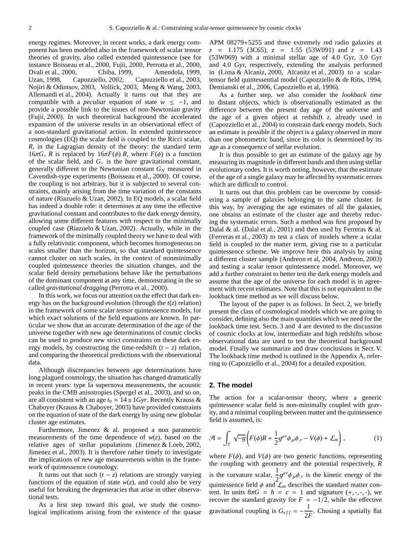
Fig. 7. The dashed line indicatesT(z) = H0t(z) according to the bestfit values of Sec. IV. for the power law potential model. The shadowedregion covers the allowed ranges coming from lookback time tests. Thevertical lines give the lowest agesTgof the considered objects for theallowed range ofh = (0.64÷0.80). The figures reported in the textcorrespond toh = 0.64, i.e. the lowest edges of the lines.For thefirst two objects, there is full agreement with the requirementT > Tg. The third age is marginally compatible, likely due tosystematics in evaluating the age-metalicity relation.

this inequality defines a dimensionless parameterTg = Hotg.In particular, for LBDS 53W091 radio galaxy discovered byDunlop et al. (Dunlop et al. 1996), the lower limit for the ageyieldstg(z= 1.55)= 3.5H0 Gyr which takes values in the inter-val 0.21≤ Tg ≤ 0.28. It therefore follows thatTg ≥ 0.21. Similarconsiderations may also be applied to the 4.0 Gyr old galaxy atz = 1.43, for whichTg ≥ 0.24, and to the APM 08279+5255,which corresponds toTg ≥ 0.131.

Only models having an expanding age parameter larger thanTg at the above values of redshift will be compatible with theexistence of such objects.

In Figs. (7), and (8) we show the diagram of the dimen-sionless age parameterT(z) = H0t(z) as a function of theredshift for two extremebest fit values of the parameters (sandH0 in the case of power law models,α3 andH0 for thequartic potential model), coming from the lookback time test.We observe that the age test turns out to be quite critical,even though such values of the parameters are fully compat-ible and equivalentto the χ2 analysis of other datasets (seeDemianski et al., 2006, Demianski et al., 2007).

In fact, it turns out that the valueTg ≥ 0.131(Friaca et al., 2005 ) atz= 3.91 is quite selective in both cases.

A remark is necessary at this point: the range of ages forquasar APM 08279+5255 is 1.8 and 2 Gyr. It is required formodels from 1011 M⊙ to 1012 M⊙ in order to reach the metalicityFe/O=2.5× solar unit (for details see Friaca et al., 2005 ).

5. Discussion and Conclusions

Cosmological models can be constrained not only using distanceindicators but also cosmic clocks, once efficient methods are de-veloped to estimate the age of distant objects. Among these,therelations between lookback time and redshiftz are particularlyuseful to discriminate among the huge class of dark energy mod-


1 2 3 4 5z

0.2

0.4

0.6

0.8

1

T

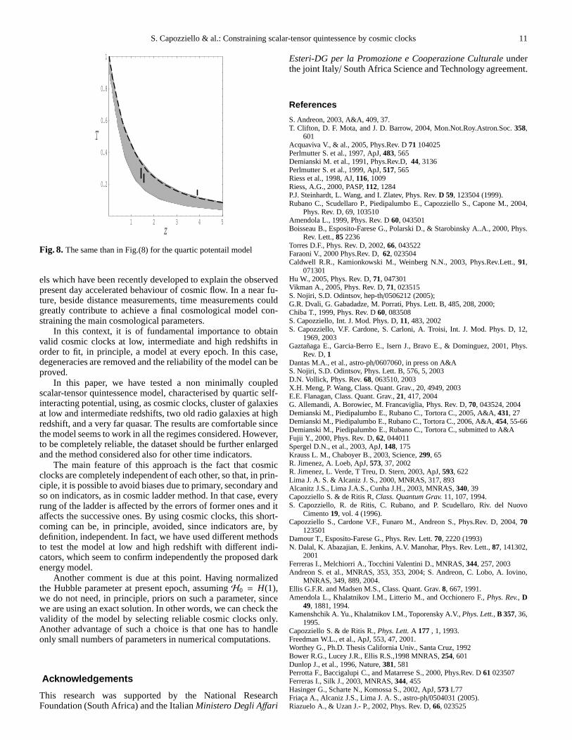
Fig. 8. The same than in Fig.(8) for the quartic potentail model

els which have been recently developed to explain the observedpresent day accelerated behaviour of cosmic flow. In a near fu-ture, beside distance measurements, time measurements couldgreatly contribute to achieve a final cosmological model con-straining the main cosmological parameters.

In this context, it is of fundamental importance to obtainvalid cosmic clocks at low, intermediate and high redshiftsinorder to fit, in principle, a model at every epoch. In this case,degeneracies are removed and the reliability of the model can beproved.

In this paper, we have tested a non minimally coupledscalar-tensor quintessence model, characterised by quartic self-interacting potential, using, as cosmic clocks, cluster ofgalaxiesat low and intermediate redshifts, two old radio galaxies athighredshift, and a very far quasar. The results are comfortablesincethe model seems to work in all the regimes considered. However,to be completely reliable, the dataset should be further enlargedand the method considered also for other time indicators.

The main feature of this approach is the fact that cosmicclocks are completely independent of each other, so that, inprin-ciple, it is possible to avoid biases due to primary, secondary andso on indicators, as in cosmic ladder method. In that case, everyrung of the ladder is affected by the errors of former ones and itaffects the successive ones. By using cosmic clocks, this short-coming can be, in principle, avoided, since indicators are,bydefinition, independent. In fact, we have used different methodsto test the model at low and high redshift with different indi-cators, which seem to confirm independently the proposed darkenergy model.

Another comment is due at this point. Having normalizedthe Hubble parameter at present epoch, assumingH0 = H(1),we do not need, in principle, priors on such a parameter, sincewe are using an exact solution. In other words, we can check thevalidity of the model by selecting reliable cosmic clocks only.Another advantage of such a choice is that one has to handleonly small numbers of parameters in numerical computations.

Acknowledgements

This research was supported by the National ResearchFoundation (South Africa) and the ItalianMinistero Degli Affari

Esteri-DG per la Promozione e Cooperazione Culturaleunderthe joint Italy/ South Africa Science and Technology agreement.

References

S. Andreon, 2003, A&A, 409, 37.T. Clifton, D. F. Mota, and J. D. Barrow, 2004, Mon.Not.Roy.Astron.Soc.358,

601Acquaviva V., & al., 2005, Phys.Rev. D71 104025Perlmutter S. et al., 1997, ApJ,483, 565Demianski M. et al., 1991, Phys.Rev.D,44, 3136Perlmutter S. et al., 1999, ApJ,517, 565Riess et al., 1998, AJ,116, 1009Riess, A.G., 2000, PASP,112, 1284P.J. Steinhardt, L. Wang, and I. Zlatev, Phys. Rev.D 59, 123504 (1999).Rubano C., Scudellaro P., Piedipalumbo E., Capozziello S.,Capone M., 2004,

Phys. Rev. D, 69, 103510Amendola L., 1999, Phys. Rev. D60, 043501Boisseau B., Esposito-Farese G., Polarski D., & Starobinsky A..A., 2000, Phys.

Rev. Lett.,85 2236Torres D.F., Phys. Rev. D, 2002,66, 043522Faraoni V., 2000 Phys.Rev. D,62, 023504Caldwell R.R., Kamionkowski M., Weinberg N.N., 2003, Phys.Rev.Lett.,91,

071301Hu W., 2005, Phys. Rev. D,71, 047301Vikman A., 2005, Phys. Rev. D,71, 023515S. Nojiri, S.D. Odintsov, hep-th/0506212 (2005);G.R. Dvali, G. Gabadadze, M. Porrati, Phys. Lett. B, 485, 208, 2000;Chiba T., 1999, Phys. Rev. D60, 083508S. Capozziello, Int. J. Mod. Phys. D,11, 483, 2002S. Capozziello, V.F. Cardone, S. Carloni, A. Troisi, Int. J.Mod. Phys. D, 12,

1969, 2003Gaztanaga E., Garcia-Berro E., Isern J., Bravo E., & Dominguez, 2001, Phys.

Rev. D,1Dantas M.A., et al., astro-ph/0607060, in press on A&AS. Nojiri, S.D. Odintsov, Phys. Lett. B, 576, 5, 2003D.N. Vollick, Phys. Rev.68, 063510, 2003X.H. Meng, P. Wang, Class. Quant. Grav., 20, 4949, 2003E.E. Flanagan, Class. Quant. Grav.,21, 417, 2004G. Allemandi, A. Borowiec, M. Francaviglia, Phys. Rev. D,70, 043524, 2004Demianski M., Piedipalumbo E., Rubano C., Tortora C., 2005,A&A, 431, 27Demianski M., Piedipalumbo E., Rubano C., Tortora C., 2006,A&A, 454, 55-66Demianski M., Piedipalumbo E., Rubano C., Tortora C., submitted to A&AFujii Y., 2000, Phys. Rev. D,62, 044011Spergel D.N., et al., 2003, ApJ,148, 175Krauss L. M., Chaboyer B., 2003, Science,299, 65R. Jimenez, A. Loeb, ApJ,573, 37, 2002R. Jimenez, L. Verde, T Treu, D. Stern, 2003, ApJ,593, 622Lima J. A. S. & Alcaniz J. S., 2000, MNRAS, 317, 893Alcanitz J.S., Lima J.A.S., Cunha J.H., 2003, MNRAS,340, 39Capozziello S. & de Ritis R,Class. Quantum Grav.11, 107, 1994.S. Capozziello, R. de Ritis, C. Rubano, and P. Scudellaro, Riv. del Nuovo

Cimento19, vol. 4 (1996).Capozziello S., Cardone V.F., Funaro M., Andreon S., Phys.Rev. D, 2004,70

123501Damour T., Esposito-Farese G., Phys. Rev. Lett.70, 2220 (1993)N. Dalal, K. Abazajian, E. Jenkins, A.V. Manohar, Phys. Rev.Lett., 87, 141302,

2001Ferreras I., Melchiorri A., Tocchini Valentini D., MNRAS,344, 257, 2003Andreon S. et al., MNRAS, 353, 353, 2004; S. Andreon, C. Lobo,A. Iovino,

MNRAS, 349, 889, 2004.Ellis G.F.R. and Madsen M.S., Class. Quant. Grav.8, 667, 1991.Amendola L., Khalatnikov I.M., Litterio M., and OcchioneroF., Phys. Rev., D

49, 1881, 1994.Kamenshchik A. Yu., Khalatnikov I.M., Toporensky A.V.,Phys. Lett., B 357, 36,

1995.Capozziello S. & de Ritis R.,Phys. Lett.A 177 , 1, 1993.Freedman W.L., et al., ApJ, 553, 47, 2001.Worthey G., Ph.D. Thesis California Univ., Santa Cruz, 1992Bower R.G., Lucey J.R., Ellis R.S.,1998 MNRAS,254, 601Dunlop J., et al., 1996, Nature,381, 581Perrotta F., Baccigalupi C., and Matarrese S., 2000, Phys.Rev. D61 023507Ferreras I., Silk J., 2003, MNRAS,344, 455Hasinger G., Scharte N., Komossa S., 2002, ApJ,573 L77Friaca A., Alcaniz J.S., Lima J. A. S., astro-ph/0504031 (2005).Riazuelo A., & Uzan J.- P., 2002, Phys. Rev. D,66, 023525

http://arXiv.org/abs/hep-th/0506212

http://arXiv.org/abs/astro-ph/0607060

http://arXiv.org/abs/astro-ph/0504031


Saini T. D., Padmanabhan T., Bridle S., 2003, Mon.Not.Roy.Astron.Soc.,343,533

Uzan J.Ph., 1998, Phys. Rev D,59, 123510Schimd C., Uzan J. P., and Riazuelo A., 2005, Phys. Rev.D 71, 083512C.M. Will, Theory and Experiments in Gravitational Physics(1993) Cambridge

Univ. Press, Cambridge.

Appendix A: The lookback time method

In order to use the age measurements of a given cosmic clockto get cosmological constraints, let us consider an objecti atredshiftzand letti(z) be its age defined as the difference betweenthe age of the universe at the formation redshiftzF , and atz:

ti(z) = tL(zF) − tL(z). (A.1)

If one is able to to estimate the agesti for i = 1, 2, . . . ,N of Nobjects, we can estimate the lookback timetobs

L (zi) as

tobsL (zi) = tL(zF) − ti(z)

= tobs0 − ti(z) − d f , (A.2)

wheretobs0 is the age of the universe (which in our units is set to

1), while the bias (delay factor) can be defined as :

d f = tobs0 − tL(zF ) . (A.3)

The delay factor is introduced to take into account our ignoranceof the formation redshiftzF of the object. Actually, to estimatezF , one should use Eq.(A.1), assuming a background cosmolog-ical model. Since our aim is to constrain the background cos-mological model, it is clear that we cannot inferzF from themeasured age, so that this quantity isa priori undetermined.Moreover we rely that it can take into account also the effect oftheGe f f variation on the age estimations, because the expectedmagnitude of such an effect. In principle,d f should be differentfor each object in the sample unless there is a theoretical reasonto assume the same redshift at the formation of all the objects.However, we can realistically assume thatd f is the same for allthe homologous objects of a given dataset (in the range of theerrors), and we considerd f rather thanzF as the unknown pa-rameter to be determined from the data.

We may then define a merit function :

χ2lt =

1N − Np + 1

ttheor0 (p) − tobs

0

σtobs0

2

+

N∑

i=1

ttheorL (zi , p) − tobs

L (zi)√σ2

i + σ2t

2,

whereNp is the number of parameters of our model,σt, σi arethe uncertainties ontobs

0 and tobsL (zi). Here the superscripttheor

denotes the predicted values of a given quantity.In principle, such a method can work efficiently to discrim-

inate between the various cosmological models. However, themain difficulty is due to the lack of available data which leadsto large uncertainties on the estimated parameters. In order topartially alleviate this problem, we can add further constraintson the model by usingpriors; for example choosing a Gaussianprior on the Hubble constant allows us to redefining the likeli-hood function as

L(p) ∝ Llt (p) exp

−12

(h− hobs

σh

)2 ∝ exp [−χ2(p)/2], (A.4)

where we have absorbedd f to the set of parametersp and havedefined :

χ2 = χ2lt +

(h− hobs

σh

)2

(A.5)

with hobs the estimated value ofh andσh its uncertainty. Weuse the HST Key project results (Freedman et al., 2001) setting(h, σh) = (0.72, 0.08). Note that this estimate is independent ofthe cosmological model since it has been obtained from localdistance ladder methods.

The best fit model parametersp may be obtained by maxi-mizingL(p) which is equivalent to minimize theχ2 defined inEq.(A.5). It is worth stressing that such a function should not beconsidered as astatisticalχ2 in the sense that it is not forced to beof order 1 for the best fit model to be considered as a successfulfit. Actually, such an interpretation is not possible since the er-rors on the measured quantities (bothti andt0) are not Gaussiandistributed. Moreover, there are uncontrolled systematicuncer-tainties that may also dominate the error budget. Moreover,thereare uncontrolled systematic uncertainties that may also dominatethe error budget. Nevertheless, a qualitative comparison of dif-ferent models may be obtained by comparing the values of thispseudoχ2, even if this should not be considered as definitiveevidence against a given model.

Given that we have more than one parameter, we obtain thebest fit value of each single parameterpi as the value which max-imizes the marginalized likelihood for that parameter, definedas :

Lpi ∝∫

dp1 . . .

∫dpi−1

∫dpi+1 . . .

∫dpn L(p) . (A.6)

After having normalized the marginalized likelihood to 1 atmax-imum, we compute the 1σ and 2σ confidence limits (CL) on thatparameter by solvingLpi = exp (−0.5) andLpi = exp (−2) re-spectively.

Documents

Constraining scalar-tensor quintessence by cosmic clocks