Embed Size (px)
Citation preview
Noname manuscript No.(will be inserted by the editor)
Constructive Model-based Analysis for Safety Assessment
Adriano Gomes · Alexandre Mota · AugustoSampaio · Felipe Ferri · Edson Watanabe
Received: date / Accepted: date
Abstract The aerospace industry still uses fault-trees to perform reliability analysis.
This is because fault-tree modeling and analysis (FTA) seems easier to practical engi-
neers when compared to Markov models, even though FTA provides a weaker form of
analysis. In this paper we propose an automatic strategy for generating Markov-based
models and corresponding analysis formulations, according to ARP 4761, directly from
Simulink diagrams annotated with failure information. The generated Markov-based
models are expressed in the formal language PRISM, and the analysis is carried out by
the PRISM model checker. The strategy is compositional and based on a comprehen-
sive set of translation rules from Simulink to PRISM. We brie�y address soundness and
completeness of the rules and, to illustrate the application of the strategy, we apply it
to a classical avionics case study: an actuator control system.
Keywords Model-based safety assessment, probabilistic model checking, markov
analysis, quantitative safety analysis, translation rules
1 Introduction
Any system is subject to failures. Critical systems, such as airplanes, autonomous
rockets, medical devices, and nuclear power plants, must work even in the case of serious
individual or multiple simple failures, because human being lives as well as considerable
�nancial assets are involved. In these systems, a rigorous safety assessment must be
applied where reliability analysis is an important aspect of this process.
A. Gomes, A. Mota and A. SampaioCentro de Informática � Universidade Federal de Pernambuco - Av. Jornalista Anibal Fer-nandes, s/n - Cidade Universitária (Campus Recife) - ZIP 50.740-560 - Recife - PE - BrazilTel.: +55-81-21268430Fax: +55-81-21268438E-mail: {ajog, acm, acas}@cin.ufpe.br
F. Ferri and E. WatanabeEmbraer, São José dos Campos, Brazil - ZIP 50.740-560 - Recife - PE - BrazilTel.: +55-81-39271000Fax: +55-12-39271000E-mail: {felipe.ferri, edson.watanabe}@embraer.com.br

2 Adriano Gomes et al.
The aerospace industry uses fault-tree analysis [1] (FTA) as a de facto standard
to accomplish safety and reliability analysis. Fault-trees are commonly employed be-
cause they are visually appealing, simple to understand, and suitable to analyze the
failure conditions and events in an isolated manner. However, most FTA approaches
present limitations, mainly concerning time aspects, because they can only capture
static information and are often created or analyzed manually, which is error-prone.
Although these di�culties are present, FTA has to be used because certi�cation
authorities only certify some categories of critical systems provided their safety and
reliability aspects are identi�ed and handled according to the accepted standards. For
instance, FTA is still the most cited approach in standards such as ARP 4754 [2], ARP
4761 [3] and FAR-25.1309 [4] for avionics systems.
Besides FTA, Markov-based analysis [5] is also accepted by certi�cation authorities.
Although Markov models and analysis do not su�er from most of the FTA limitations,
the industry rarely adopts Markov models because they are considered too complex
to be created and handled. Even with the recent advances in model-based solutions
towards system design [6,7,8], there seem to be no model-based approaches able to
perform safety analysis systematically and e�ciently, mainly using Markov analysis,
adopted by industry.
In this paper, we both improve and extend a strategy, originally presented in [9], for
automatically generating Markov-based models, as well as the formulation for their me-
chanical analysis, directly from Simulink diagrams annotated with failure information;
the driving motivation is to perform quantitative safety assessment of aircraft sys-
tems. We use the formal language PRISM [10,11] as an intermediate notation between
Simulink [12] diagrams and Markov models. PRISM has a simple and compositional
textual representation for Markov-based models as well as a very �exible tool support
able to investigate di�erent safety aspects of a Markov model.
The major new contributions with respect to [9] are the following.
� We present a more comprehensive set of translation rules than that presented in [9].
Furthermore, based on induction of the Simulink model structure, we address the
completeness of the proposed set of rules.
� We also address soundness to some extent. Particularly, the rules are shown to be
sound in the sense that their applications generate Markov models (from anno-
tated Simulink diagrams) which are consistent with some guidelines and patterns
provided by ARP 4761.
� We have mechanized the entire strategy, including the generation of Markov models
from Simulink diagrams as well as the automatic formulation of relevant properties,
according to ARP 4761, which are veri�ed by the PRISM model checker.
The COMPASS project [8] and the work on pFMEA [13] are closely related to ours.
The former performs probabilistic safety assessment using a design language named
SLIM (System-Level Integrated Modeling). Similarly to our proposal, the COMPASS
project includes tool support and notions of completeness and consistency. However,
the user has to deal with the language SLIM directly, as opposed to our proposal that
keeps the formal language behind the scenes, easing its adoption by engineers. The
work on pFMEA also uses the PRISM model-checker. In one sense, pFMEA performs
a more detailed analysis than ours because it considers faulty as well as normal be-
haviors of a system. Nevertheless, the models proposed by pFMEA are not generated
systematically (which is potentially error-prone) and these models are more suscepti-
ble to state explosion because its PRISM speci�cation is too detailed (it handles each

Constructive Model-based Analysis for Safety Assessment 3
Fig. 2.1 Safety assessment overview
situation of the system controller variables, that describes its nominal behavior, as a
possible Markovian state).
This paper is organized as follows. The next section presents an overview of the
proposed quantitative safety assessment process; we also introduce the formal language
PRISM and how to model and perform safety analysis using PRISM. In Section 3 we
present a complete set of rules that translate a Simulink diagram, annotated with
a failure logic, into a PRISM model to perform quantitative safety assessment. We
then intuitively address soundness, in Section 4, by comparing some representative
patterns used by ARP 4761 to perform safety assessment using Markov chains with
corresponding PRISM models generated by our translation rules. To potentialize the
introduction of our proposal in the aerospace industry, in Section 5 we consider tool
support. We present a practical demonstration of our proposal in Section 6, where a
real case study is considered. Finally, we detail some related work in Section 7 and our
conclusions and future work in Section 8.
2 Quantitative Safety Assessment using PRISM
The proposed strategy is summarized in Figure 2.1. We �rst consider a Simulink dia-
gram modeling a system, where its goal is to characterize the nominal (normal) aspects
of such a system. By augmenting this Simulink diagram with modular failure informa-
tion (adding failure logic for each component), we have the nominal as well as the
failure behavior of the system. To this augmented Simulink diagram, we apply a series
of translation rules in the sequence described in Figure 3.2 to obtain a failure proba-
bilistic model of the system expressed in Continuous Time Markov Chain (CTMC) and
speci�ed in PRISM as well as several criticality questions, representing desired safety
properties of this system. Finally we use the PRISM model checker to verify whether
any of these questions is violated. We can further investigate more dynamic aspects of
the failure behavior of this system by performing experiments.
2.1 Overview of Quantitative Safety Assessment
The safety assessment process involves complex phases and activities [3], aiming to
minimize the occurrence likelihood of potential hazards. During this process, failure
analysis is performed in parallel with system design for ensuring that the occurrence of

4 Adriano Gomes et al.
possible hazard situations of the system must be unlikely. As a result, safety require-
ments are introduced in the top-level and subsystem design, considering qualitative
and quantitative aspects. They comprehend the high-level airplane goals as well as
system safety goals that must be considered in the proposed system architectures.
Qualitative and quantitative analysis must be performed over the proposed system
design to ensure that all the introduced safety requirements are met. In particular,
the quantitative assessment is a more complex and laborious task because it deals
with more rigorous and accurate constraints [4]. In this paper we focus on quantitative
assessment.
Certi�cation authorities accept FTA, Markov analysis or dependence diagrams as
alternatives to perform quantitative safety assessment. The basic information used
as input to these techniques are failure conditions and failure rates. A failure rate
is an attribute used to model the likelihood of each basic failure mode (primary and
independent failure) of the system. Failure conditions are events of the system (hazards)
whose occurrence may lead to a critical situation. They are identi�ed during the FHA
(Failure Hazardous Analysis), which considers the severity of each failure condition
occurrence over the system functions to de�ne the related safety requirements, using
an argument (maximum tolerable probability). For example, FHA determines that the
probability of occurrence of a catastrophic failure condition must not be greater than
10−9 per �ight hour [4,3].
However, it is necessary to identify the failure logic of the system before perform-
ing a qualitative or quantitative assessment. Therefore, a systematic examination of
the proposed system architecture is performed to determine which single failures or
combination of failures can exist at the lower levels of the system that might cause the
occurrence of each failure condition. This examination follows a top-down evaluation
along the subsystems and components of the system, identifying and determining the
logic relation between the failure modes of each component/subsystem in relation to
their respective failure conditions. At component level, it uses the quantitative values
obtained from the Failure Modes and E�ects Summary (FMES) to supply the failure
rates considered in each system component. The FMES is a summary of failures iden-
ti�ed by FMEA (Failure Mode E�ective Analysis). FMEA is a bottom-up method for
assessing the failure modes of a system and determining the e�ects of the relations
among these failures.
Accordingly, an assessment to identify and classify the failure conditions as well as
determining the logic relation between its single failures is necessarily qualitative. On
the other hand, an assessment of the probability of a failure condition, considering its
single failures may be quantitative. Therefore, essentially, a quantitative assessment
aims to make reliability predictions for the system. For the certi�cation of an aircraft,
the recommended analysis methods (FTA, Markov Analysis or dependence diagrams)
consider the failure logic of the system and calculate the average probability of all
identi�ed failure conditions (per �ight hour), assuming the appropriate exposure time
of failures, to show if the results are tolerable.
2.1.1 Model-based Safety Assessment
In the safety-critical systems domain there is an increasing trend towards model-based
safety assessment [14,15]. The idea is to extend the existing model-based development
activities (simulation, veri�cation, testing and code generation), which are based on a

Constructive Model-based Analysis for Safety Assessment 5
Fig. 2.2 Overview of a compositional model-based safety analysis
high-level model of the system (expressed in a notation such as Simulink or Statem-
ate [16]), to incorporate safety analyses. These new alternatives are proved promising
because they are simple, compositional and do not depend on the engineer's skills to
be applied. In addition, they can use formal methods, for instance theorem provers,
model-checkers and static-checkers [15,17], to automate, even if partially, the analysis.
Moreover, formal methods are one of the alternative methods proposed in DO-178B [18]
for the airborne software certi�cation.
Most model-based strategies for safety assessment are mainly based on FHA and
FMEA [14] (and in particular on its newer variant, IF-FMEA � Interface-Focused
FMEA [19,20]). IF-FMEA is of particular interest because it uses a hierarchical tabular
structure very useful to capture the transformation and propagation of failures in a
system, allowing that complex systems can be modeled in a compositional way as well
as be easily incorporated into a design tool like Simulink, using annotations [21].
The support for a graphical notation allows modeling complex systems as hierar-
chies of architectural diagrams that can be represented either as components or sub-
systems. When an architectural block diagram is rendered as a subsystem, it can be
further explicated in terms of more basic components whose failure behaviors can be
determined. When a diagram is represented as a basic component, its failure behavior
is known, and it can be recorded in an IF-FMEA table (see Figure 2.2). From the fail-
ures of all basic components, we can determine how the functional failures, which were
identi�ed in exploratory analysis of the FHA, arise following the combination of failure
modes recorded in IF-FMEA tables. As illustrated in Figure 2.3, an IF-FMEA table
records how a component reacts to failures generated by other components and sets the
failure modes of the component itself as well as its propagation to other components.
The table in Figure 2.3 records four pieces of failure based information and a
descriptive �eld: Output Failure Mode represents the possible failure modes of a
component, Description contains a brief explanation of the failure mode, Input De-
viation Logic has the dependency of such failure modes with respect to the identi�ed
failures via their input ports as boolean expressions, Component Malfunction de-
scribes what happens upon a certain failure mode occurrence, and λ (f/h) holds a
failure rate for each input port used in the Input Deviation Logic expression.
In this sense, additional information can be incorporated to these tabular structures
aiming to proper detail the safety analysis. The table in Figure 2.4 presents a fragment
of the additional failure analysis information about the failure monitoring of the system,
besides de�ning the relevant exposure times (e.g. time intervals between maintenance
and operational checks/inspections) of each component.

6 Adriano Gomes et al.
Fig. 2.3 IF-FMEA of a hypothetical component system
Fig. 2.4 Fragment of additional failure analysis information
The additional information is recorded through: theMaintenance Strategy �eld
which represents the classi�cation of each basic component of the system about its
failures' monitoring. In the aeronautics context, some components are checked before
each �ight to con�rm that they are working, and repaired if necessary. So, a compo-
nent is called as self-monitored, if one needs to know whether it is working properly
before each �ight. But some aircraft systems include components that are not inspected
before and during every �ight. Failures in such components are called latent because
they are not detected unless another combined failure occurs, compromising a function
that needs such components, or during scheduled maintenance (generally, after some
�ights). For this last type of component we must consider two classi�cations: monitored
and non-monitored components. A component is named monitored if it is continuously
monitored by an independent monitor (mapped by the Associated External Port
�eld). If the component fails and the monitor is working, the component can be re-
paired before the next dispatch. If the monitor is not working, latency reappears.
The type monitor is a particular component responsible for monitoring other relevant
components. The non-monitored classi�cation represents all components that are not
monitored and can naturally present latent failures; their faults are only checked in
regular periods of maintenance. Based on reliability predictions and safety factors (dis-
patchability, MTBF � Mean Time Between Failure, severity, redundancy, and other
several reasons) the periodic inspection/repair intervals for each component are also
de�ned (Inspection Time �eld).

Constructive Model-based Analysis for Safety Assessment 7
2.2 Markov Modeling and Analysis
After identifying the failure conditions in the FHA and performing a compositional
safety analysis, the FTA/DD/MA can be applied to determine which single or com-
bination of failures can exist (if any) at the lower levels that might cause each fail-
ure condition and calculate the failure condition probabilities. Combinatorial analytic
models like reliability block diagrams and fault trees are similar in that they capture
conditions that make a system fails in terms of the structural relationships between
the system components. If in each component we annotate its:
� Failure modes and respective rates
� Exposure time
� Failure logic
and assuming that its failure modes are statistically independent, it is possible to create
a failure model (fault-tree) of the system following its de�ned architecture [3]. Then,
this model can be applied to determine the probability of undesired failure conditions.
In a model-based context, we can create such a model automatically, because the system
components augmented with their failure arguments were de�ned in a compositional
style, allowing an intuitive and systematic synthesis of the failure model based on
the system failure logic. The work presented in [22,19] is a classical example of this
approach and is also used as basis of our strategy for creating Markov models.
Creating a Markov model is potentially more complex than modeling fault trees;
it considers more complicated interactions between components. Several examples of
dependencies among system components have been observed in practice and can be
captured by Markov models. In a reliability view, failure/repair dependencies are often
present (e.g., shared repair, warm/cold spares, imperfect coverage, non-zero switching
time, travel time of repair person, reliability with repair) [3].
However, according to ARP 4761, the methods to assess the reliability and safety
of a system, in a quantitative view, can be separated in two categories:
� Fault Occurrence and Repair Model (FORM);
� Fault and Error Handling Model (FEHM).
The former deals only with the situations where the system fail and repair strategies
are involved. In this case a perfect coverage of failures is assumed. So, the system can
detect any fault that can happen and recon�gure itself to a degraded mode instanta-
neously. The system behavior is described by means of fault-trees or Continuous-Time
Markov Chains (CTMC). The latter de�nes the system behavior after a fault occur-
rence. The Fault and Error Handling Model can be used to model the complex actions
and interactions in the system when a fault occurs. In the FEHM, imperfect coverage
is assumed, because there could be several decisions to be made and modeled such as:
fault detected, fault isolated, system recon�gured, system repaired and system failure
due to a near coincident fault.
The FORM model is easier to use and apply into a model-based safety assessment
context because it can be often performed over all subsystems and components included
in the safety assessment process. Contrarily, FEHM can only in general be performed
over speci�c systems (because the information needed to make this kind of modeling is
hardly available for all subsystems and components). For these reasons, our approach
is based on FORM. Therefore, in this section we describe how to model Markov chains

8 Adriano Gomes et al.
Fig. 2.5 Markov chain of two components in parallel
assuming the FORM model and how the system reliability information is related with
this model1.
A Continuous Time Markov Chain is a state-space based (stochastic) model. A
state in such a model represents a combination between fault-free and faulty com-
ponents information as well as system redundancy information. Transitions between
states represent possible changes of the system state due to the occurrence of events.
A transition can use a simple (a single component participates) or a compound event
(more than one component participate). A Markov analysis calculates the probabil-
ity of the system to reach a certain state as a function of time. In the continuous
time framework, the model is characterized by discrete states and exponential time
distributions that determine the rate of each transition.
The standard representation of a Markov chain is given by a state transition dia-
gram, suitable for graphical representation, or a transition matrix, used for calculations.
The state transition diagram shows the number of possible states and transition rates
between them. To illustrate the operation of Markov chains, we consider, for instance,
a simple case of a system with two possible states (see Figure 2.5): operating system
(available) and failure (system unavailable). In this case, transitions between these
states could represent the failure and repair processes to which the system is subject.
Therefore, the dynamic behavior of the system can be regarded as a sequence of states
evolving in time. Figure 2.5 shows such a system. It consists of two components (A
and B) in parallel. As each component has two states, the system in parallel has four
possible states. The states represent an operational or non-operational status of the
system components. So, a system changes its state due to events such as component
failure or completion of repair. Each state transition is a random process represented
by a speci�c di�erential equation. So, a transition from one state to another occurs at
a given transition rate that is a function of the failure or repair rate. This system is
operational (available) when at least one of these components is working properly.
In a real situation, repair is a discrete process (performed at maintenance sched-
ules or check intervals). However, models approximate discrete repairs by stochastic
1 This section presents an intuitive understanding of Markov analysis without the complexityof the underlying mathematics.

Constructive Model-based Analysis for Safety Assessment 9
processes. This approximation is permitted by certi�cation authorities, when the com-
ponents failure rates are much lower than the repair rates (in order of magnitude).
Markov chains are not limited to sequential structures. As shown in Figure 2.5,
multiple transitions can occur from a single state. The model allows a direct transition
from the state 0 to state 3. Within the context of reliability, this transition could
represent the simultaneous failures of two components (due to a common cause failure
of these components), resulting in immediate unavailability of the system. Thus, there
is the possibility of characterizing both independent and dependent failures while the
system is in state 0.
The quantitative evaluation of the behavior of Markovian processes is captured
by the Chapman-Kolmogorov equation [5]. The solution of this equation gives the
probability of the unconditional state (determining the probability of a state without
depending on the probability of others). This temporary solution is very signi�cant
when the system under investigation must be evaluated with respect to its behavior
in the short term. Assuming long term (known as steady state), however, it can be
shown that the state probabilities often converge to constant values. These stationary
(equilibrium) state equations can be derived from the system of di�erential equations
that expresses the appearance and disappearance of a state as relative to other states,
through a statistical equilibrium [5].
CTMC can be analyzed using two traditional properties: transient behavior, which
considers the state of the model at a particular time instant; and steady-state behavior,
which describes the state of the CTMC in the long-run.
The state equations for any system can be constructed by inspection of the Markov
chain. However, due to mathematical complexity, Markov models are commonly solved
using fast algorithms assuming stochastic independence between the occurrence of
system events [23]:
� Sum of Disjoint Products (SDP) algorithms;
� Binary Decision Diagrams (BDD) algorithms;
� Multi-terminal binary decision diagrams (MTBDD) algorithms;
� Direct or Interactive Methods (Gaussian elimination, Jacobi, Gauss-Seidel, SOR);
� Factoring (conditioning) algorithms;
� Series-parallel composition algorithms;
� Hybrid composition algorithms.
These algorithms are now available in several model-based solutions (model-checkers)
[24,17,8,10].
2.3 PRISM: A Markov-based framework for modeling and analysis
Several formalisms have been proposed for specifying probabilistic models [25,26,27].
Nowadays, PRISM [10,11] is one of the most prominent formalisms, because it pro-
vides a simple, textual modeling language, based on the concept of reactive modules
as de�ned by Alur and Henzinger [28]. It is the only formalism that speci�es and ana-
lyzes Markov models described with discrete time (DTMC), continuous time (CTMC),
Markov decision processes (MDP), Probabilistic automata (PA), or Probabilistic timed
automata (PTA) using e�cient and feasible techniques to represent states of complex
systems.

10 Adriano Gomes et al.
Fig. 2.6 The structure of PRISM
Figure 2.6 illustrates how Prism works in the case of a CTMC model: �rst, it reads
and analyzes a system's description written in formal speci�cation language. Then it
builds the corresponding representation in CTMC, calculates the set of all reachable
states, and identi�es any deadlock states (that is, absorbing states). Then PRISM
analyzes all properties in CSL [29] determining if the model satis�es each property.
The underlying data structures in PRISM are BDD (Binary Decision Diagram)
[30] and MTBDD (Multi-Terminal Binary Decision Diagram) [31]. However, the tool
provides three di�erent engines that can be used for numerical computation (a conven-
tional explicit version using sparse matrices, a pure MTBDD-based implementation,
and a hybrid approach considering both).
2.3.1 Model speci�cation
Modules and variables are the basic ingredients of this language. A system is built
from the parallel composition of a set of modules. Modules can interact with each
other (synchronization) and contain a number of variables that re�ect their possible
states. Variable datatypes include: integers, reals and booleans. They can be declared
locally or globally. The behavior of a module (the changes between its possible states
via quanti�ed transitions) is determined by a list of guarded commands. For a CTMC,
a command uses the following syntax:
[action] <guard> � rate : <update>;
Each command (initiated by a [], possibly with a label inside) is formed of a guard
(boolean expression before the symbol ->, which is a predicate over the model variables)
followed by a rate or probability (a non-negative real-valued expression, where 1 means
100%) and the update expression gives new values to local variables in the module
following this syntax:
(v1' = u1) & (v2'= u2) & . . . & (vk'= uk)
where v1, v2, . . . , vk are local variables of the module and u1, u2, . . . , uk are expres-
sions over these variables. The prime symbol (') indicates the variable (state) after the
transition is performed. A module can access all variables of the model, including the
global ones, but it can only update its own local variables. So, each command creates
a state transition.
The modules are integrated typically using the standard CSP [32] parallel compo-
sition operator (that is, modules synchronize over all their common actions). PRISM
also supports other CSP process-algebraic operators (alphabetized parallel, interleav-
ing, etc) that can specify more precisely the synchronization between modules.

Constructive Model-based Analysis for Safety Assessment 11
Fig. 2.7 Left: A Markov chain modelling a parallel system - repairable. Right: correspondingPRISM code.
A command (belonging to any of the modules) is enabled in a global state of
the probabilistic model provided the current state satis�es the predicate guard. If a
command is enabled, a transition that updates the module variables can occur with
the given rate. For CTMC, the choice between which command is performed (that is,
the scheduling) depends on the race condition. The multi-way synchronization provides
interactions between multiple modules, that is, simultaneous changes in their states. It
is modeled by augmenting guarded commands with action labels that are placed inside
the square brackets.
Furthermore, PRISM also provides the operator formula. A formula is a boolean
expression that can be composed by a set of module variables associated with basic
logical operators ( NOT: !, AND: &, OR: | ). A formula can be used to label certain
states of the system, helping to de�ne the guard of the module commands, as well as
creating useful expressions to evaluate the system.
Figure 2.7 illustrates the PRISM speci�cation corresponding to the Markov chain
and Simulink diagram shown in Figure 2.5.
The �rst line of this speci�cation states that we are considering a continuous time
Markov chain that is composed of a set of discrete states, where each of them is the
representation of the state (operational, degraded and faulty) of each failure mode
(local variables) of the system components. This chain of events requires the use of
exponential probability distributions for modeling failure mode rates and repairs (this
is why we use the CTMC model).
In PRISM, each module can represent a subsystem or component of the system. So,
the speci�cation in Figure 2.7 comprises two modules that represent the components

12 Adriano Gomes et al.
Fig. 2.8 Markov models and corresponding PRISM representation of three basic cases of thepossibles system arquitectures: a serie system (non-repairable), a serie system (repairable) anda parallel system (non-repairable) respectively.

Constructive Model-based Analysis for Safety Assessment 13
A and B composed in parallel. The �rst module, Component B, contains a boolean
variable b failed that represents its single failure mode (false = operational, and true
= failed). The �rst transition captures one of the possible changes in the failure mode:
from an operational state it can fail with a rate of 5.10−4 (failure/hour). The next
command represents a repair transition. The last two commands are synchronized (the
labels inside [ and ] state the synchronization points) with the module Component A.
They work similarly to the other transitions of this module, except that they need to
synchronize with the corresponding labels of the module Component A, allowing them
to be triggered. The module Component A also uses a single variable: a failed. Its �rst
command states a failure transition command whereas the second represents the capa-
bility of its single failure mode being repaired with a rate of 1/50 (repair/hour). The
last two commands represent a repair transition synchronized with the Component B.
Finally, the formula system failure represents the system failure state in the format of
a boolean expression.
Note that the example shown in Figure 2.7 represents one (a parallel system -
repairable) of the four basic cases of a system architecture and the way how the Markov
chain should to be modeled as recommended by ARP 4761 [3]. The left-hand side
shows the corresponding Markov chain resulting from the semantics of the PRISM
speci�cation. As it can be seen, this diagram is identical to the diagram presented in
Figure 2.5. The other three cases (a parallel system � non-repairable, a series system
� repairable, and a series system � non-repairable) are represented in Figure 2.8,
including their corresponding PRISM speci�cations. In practice, a complex system (real
system) is a combination of these four simpler systems. Therefore considering that the
PRISM model can grow just by adding new modules (because its own speci�cation can
handle a module composition), it is intuitive to see that PRISM supports the FORM
modeling appropriately [3,30].
2.3.2 Model Analysis using PRISM
To analyze the failure behavior of a stochastic model, we can use, depending on the
purpose, a steady-state or transient analysis [5]. Transient analysis represents the in-
stantaneous failure rate over a single period T whereas the steady-state (equilibrium
state) analysis approximates the long-term average failure rate. The choice over these
types of analyses depends on how system repairs are handled. Transient analysis can
be performed in either closed-loop (models with repairs) or open-loop models (models
without repairs), whereas the steady-state analysis can be performed only on closed-
loop models.
Recall from Section 2.2 that the proposed failure model considers repair transitions
as if they occurred at constant rates. That is, we are assuming a typical closed-loop
model and both analyses can be performed. We calculate the average rate of a failure
condition applying the transient analysis. Particularly, transient analysis with contin-
uous repair provides adequate accuracy on their results for our purposes, since most
critical systems are modeled in such a way that they can deal with latency. In this
scenario, several components a�ecting the system functionality must be monitored,
maintained at regular intervals and repaired if they are faulty and the transient anal-
ysis with continuous repair is more representative in this situation [4,3]. Comparing
with the steady-state analysis, the transient behavior during the �rst several hours is
insigni�cant, requiring more care for the engineers to perform the analysis appropri-
ately. But the instantaneous rate of the transient analysis generally has already come

14 Adriano Gomes et al.
close to the asymptotic steady-state rate in few hours and can be explored in speci�c
time instants rather than steady-state that only analyses the long-run situation (it is
not useful in the aircraft context). Moreover, a transient analysis can determine the
contour condition of the instantaneous failure rate as a function of time, showing the
system sensitivity. A steady-state analysis does not provide this information.
To perform a quantitative safety analysis, PRISM uses the CSL language [29]. The
operators S (steady-state) and P (transient) of PRISM are used to reason about the
tolerable probabilities of all system failure conditions. For example, with the expression:
S <= 10−9 [ �Failure Condition� ] (1)
we can check if, in the long run, the probability that a certain �Failure Condition�
can occur is less than or equal to 10−9. In this case,"Failure Condition� is usually
a formula de�ned in the PRISM speci�cation. Note that the evaluation of such an
expression yields "yes" or "no", based on the corresponding quantitative analysis (the
value is implicit). We can also check the exact probability itself by using another CSL
formula
P = ? [ true U<=3600 �Failure Condition� ] (2)
This yields the instantaneous probability of occurrence of a certain �Failure Condition�
within 3600 time units.
Therefore, PRISM can support both analysis solutions (steady-state or transient
analysis). However, as the steady-state analysis value is considered to a limit situation
(equilibrium state), to calculate the average probability of a failure condition on the
situation where the equilibrium state is not achieved during the lifetime of the system,
we should apply another formula in PRISM using the transient operator normalized
with a speci�c time T:
((P = ? [ true U<=T "Failure Condition" ])/T) (3)
Following this principle, we can also check if the probability that a certain "Failure
Condition" can occur is less than or equal to 10−9 using the transient operator:
((P = ? [ true U <= T "Failure Condition" ])/T) <= 10−9 (4)
As we pointed out previously, Formulas 3 and 4 are more appropriate to analyze
our models.
3 A Complete Set of Translation Rules
In this section we present a set of translation rules that takes a Simulink diagram,
annotated with failure information, and creates a PRISM model on which one is able
to perform a quantitative safety analysis of the desirable properties. We also consider
some restrictions our rules are not currently tackling as well as a notion of relative
completeness for our set of rules.

Constructive Model-based Analysis for Safety Assessment 15
System ::= Diagram
Diagram ::= System Name × seq(SubSystem)
SubSystem ::= Component | DiagramModule ::= Module Name × seq(Deviation)
× seq(FailureMode)× seq(Port)
×MaintenanceStrategy × InspectionTime
Port ::= Port ID ×AssociatedPort
Deviation ::= Deviation Name × Port ID
×Annotation × Criticality
FailureMode ::= FailureMode Name × Rate ×Annotation
MaintenanceStrategy ::= MS Type × seq(AssociatedPort)
MS Type ::= Self Monitored | Monitored
| Non monitored | Monitor
Port ID ::= In〈〈N〉〉 | Out〈〈N〉〉AssociatedPort ::= empty | Module Name × Port ID
Annotation ::= empty | FailureMode Name
| Deviation Name × Port ID
| And〈〈Annotation ×Annotation〉〉| Or〈〈Annotation ×Annotation〉〉
Criticality ::= empty | RInspectionTime ::= RRate ::= R
Fig. 3.1 Abstract syntax based on tabular annotations
3.1 Input Data Model
Although failure annotations of a Simulink diagram appear in tabular structures, our
rules are based on the grammatical structures of Figure 3.1. We developed a tool [33],
as presented in Section 5,that translates failure annotations, according to Figure 3.1,
into a PRISM model, from which one can calculate the failure probability of the top
event as well as other reliability calculations.
According to the grammar de�ned in Figure 3.1, a system is de�ned as a diagram
that has a name (System Name) and a list of subsystems (seq (Subsystem)). Each
subsystem can be another diagram or a module (Components can also be systems).
These elements are used mainly to generate the modules of the proposed PRISM spec-
i�cation. A module (Module) represents the lower level component that has a name
(Module Name), a list of deviations (seq (Deviation)), a list of failure modes (seq
(FailureMode)), a list of ports (seq (Port)), information about the maintenance strategy
(MaintenanceStrategy) and the inspection time (InspectionTime). All these elements
are associated with the tabular structures used to store all system information about its
architecture, hierarchy, failure conditions, failure modes, repairs and the characteristics
of monitoring and propagation of component failures. In the proposed PRISM speci�ca-
tion, these elements compose the body of each module. A port (Port) is a structure that
contains its identi�er (Port ID) (representing the identi�er of input/output ports) and
an associated port (AssociatedPort), which stores the connected port of another com-
ponent. A deviation (Deviation) is represented by its name (Deviation Name), a port
16 Adriano Gomes et al.
identi�er, a logic based annotation (Annotation) and its criticality (Criticality). The
property expressions of the proposed PRISM model are generated mainly with these
elements. A failure mode (FailureMode) is captured by its name (FailureMode Name),
its failure rate (Rate) and its trigger condition (Annotation). Subsequently, we have
the maintenance strategy (MaintenanceStrategy) that is formed of a pair whose �rst
element is the type of the strategy (MS Type) and the second one is a list of associ-
ated ports (AssociatedPort). The maintenance strategy is provided using the following
types: self monitored (Self Monitored), monitored (Monitored), non-monitored at all
(Non Monitored), and monitor (Monitor). The failure and repair commands of each
module in the proposed speci�cation are generated mainly with these elements. A port
identi�er is simply a tagged data type (to characterize an input or output port) of
natural numbers (In〈〈N〉〉 or Out〈〈N〉〉). An associated port is a pair formed of a name
and of a port identi�er or the element empty , which means no associated port. An
annotation is a boolean expression that represents the failure logic of deviations. Its
de�nition considers And/Or operators and their terminals can be failure mode names
or deviations from any port. An annotation can also be empty to denote no condi-
tions at all. These elements are used mainly to generate the formulas of the proposed
PRISM speci�cation. Criticality represents a real number (R) used to quantify the
tolerable probability associated with a failure condition (expressed via a deviation)
or the element empty , which characterizes a non-critical function. Finally, Rate and
InspectionTime are also real numbers used to represent the rate of occurrence of a
failure mode and of a repair, respectively.
3.2 Translation Rules: Overview and Completeness
We present 38 translation rules. These rules are applied following the order illustrated in
Figure 3.2 and they gradually create a (textual) PRISM speci�cation that captures the
failure behavior of the intended system from a Simulink diagram annotated with failure
information. By compiling such a PRISM speci�cation one obtains a corresponding
Markov-based model, on which one can perform several di�erent analysis. Particularly,
one can investigate whether speci�c CSL formulas, which we also create automatically,
are violated or not. When a formula is violated, this means that the reliability of a
certain function of the system is not achieved as required by the certi�cation authorities.
In this case, the system design must be updated by the engineering team and the
translation and subsequent analysis repeated accordingly.
Our rules are complete in the sense that they can translate any Simulink diagram,
with a failure logic in the IF-FMEA style, provided the model does not consider bidirec-
tional data �ows (such as the propagation of failure as short-circuit). Yet, such features
can be added by considering new translation rules.
The strategy always starts by applying Rule 1, which states that we are dealing with
a CTMC Markov model and applies other rules to create the several PRISM modules
from the system components (Rules 2-5). The body of a module is e�ectively created by
Rule 6. After that, basic declaration instructions (Rules 7-8), commands (Rules 9-10)
and repair transitions (Rules 11-16) are created. To complete the translation strategy,
formula expressions are created (Rules 19-24) using a set of rules that decomposes all
logic expressions (Rules 25-31). Complementing the PRISM model, the CSL formulas
used to perform safety assessment are created by Rules 32-38.

Constructive Model-based Analysis for Safety Assessment 17
Fig. 3.2 Sequence of translation rules application
Each of the following subsections addresses the translation rules for related elements
of the input data model.
3.3 Compound Systems and Subsystems
Our rules are inductively de�ned on the structure of the syntax given in Figure 3.1. We
start with Rule 1 that takes as argument a pair (a diagram) whose �rst element is the
name of a system (SName) and the second element a list of its subsystems (SubSys).
It is worth observing that this rule demands at least one subsystem (SubSys 6= 〈〉).
Rule 1 [[(SName,SubSys)]]System Ictmc
[[(SName,SubSys)]]Diagram
proviso SubSys 6= 〈〉
Following Rule 1, the resulting PRISM code is basically the directive ctmc (in-
structing PRISM to perform a Continuous Time Markov Chain interpretation), and
the actual processing of the diagram is delegated to Rule 2, which itself delegates to
Rule 3, Rule 4 or Rule 5, depending on the list of subsystems (SubSys). The term
SName is only used to de�ne the �le name of the speci�cation (But this is operational
and thus not stated in the rule).

18 Adriano Gomes et al.
Rule 2 [[(SName,SubSys)]]Diagram I [[SubSys]]Subsystem
Rule 3 applies when the list of subsystems has a single element, represented by
the singleton sequence 〈S〉 below, and this element is a module. In this case, this rule
delegates to Rule 6 that deals with modules.
Rule 3 [[〈S〉]]Subsystem I [[S ]]Module
proviso S = (MName,Type,Devs,FailureModes,Ports,MStrat , IT )
If, on the other hand, the single element is not a module then it must be a diagram
(a hierarchical description). In this case, Rule 4 applies.
Rule 4 [[〈S〉]]Subsystem I [[S ]]Subsystem
proviso S = (SName,SubSys)
Finally, we have the general situation of a list of subsystems. Rule 5 then handles
the constituent elements of the list.
Rule 5 [[〈S〉a SS ]]Subsystem I[[〈S〉]]Subsystem
[[SS ]]Subsystem
Except for Rule 1, none of the previous rules creates any PRISM code. They in-
ductively act on the structure of Figure 3.1, generating patterns for subsequent rules
to produce PRISM code.
3.4 Module
Rule 6 creates a PRISM module from a Simulink module. It receives a Simulink module
as its tuple detailed representation: the module's name (MName), list of deviation logics
(Devs), list of failure modes (FailureMode), list of ports (Ports), maintenance strategy
(MStrat) and inspection time (IT ). The module's name is used to name the PRISM
module (between the keywords module and endmodule). Inside the module, the �rst
term is dealt with by Rules 7 and 8, which create the declaration part; the following
two terms are handled by Rules 10-22, which deal with the behavioral part, formed of
failure (function FailCmds) and repair commands (function RepairCmds). Finally, the
last term is handled by Rules 23-38, which create the set of PRISM formulas outside the
module. It is worth noting that the proviso of Rule 6 requires that at least one failure
mode exists (FailureModes 6= 〈〉). Similarly, there must exist at least one deviation
logic, one port and one maintenance strategy.
Rule 6 [[(MName,Devs,FailureModes,Ports,MStrat , IT )]]Module ImoduleMName
[[(MName,FailureModes)]]Decls
[[(MName,FailureModes)]]FailCmds
[[(MName,Ports,FailureModes,MStrat , IT )]]RepairCmds
endmodule
[[(MName,Ports,Devs)]]Formulas
proviso FailureModes 6= 〈〉, Devs 6= 〈〉, Ports 6= 〈〉 and MStrat 6= 〈〉

Constructive Model-based Analysis for Safety Assessment 19
3.5 Declarations
Failure Modes are representations of possible failures within a component. To capture
this feature in PRISM, we use local boolean variables whose names are created from the
name of a module (MName) followed by the name of the failure mode (FmName) itself.
These variables are initialized with false, meaning this failure mode did not occur yet.
The creation of the declarations of such local variables is performed by Rules 7 and 8.
Rule 7 addresses the base case of a single failure mode.
Rule 7 [[(MName, 〈(FmName,Rate,Annot)〉)]]Decls IMName. .FmName : bool init false;
To deal with the general case of lists with two or more failure modes Rule 8 is
applied.
Rule 8 [[(MName, 〈(FmName,Rate,Annot)〉a FailureModes)]]Decls IMName. .FmName : bool init false;
[[(MName,FailureModes)]]Decls
3.6 Failure Transition Commands
The previous section considered the declaration of local variables for each failure mode
of a component. To characterize the occurrence of such a failure mode, the following
rules create PRISM commands. Rule 9 deals with an empty list of failure modes in
which case it does not produce any PRISM code at all (represented by ε in this rule).
Note that the base case of Rule 7 is a singleton failure mode, since PRISM does
not allow modules with an empty list of declarations; in the case of Rule 9 and of
other rules in the sequel, the base case is an empty list, since PRISM allows that no
commands are associated with a declaration.
Rule 9 [[(MName, 〈〉)]]FailCmds I ε
Rule 10 handles the general case of a non-empty list of failure modes. For the head
of the list, this rule always assumes the guard as a logical conjunction between the
negation of a failure mode (recall that the previous section initialized these variables
with false). If such a guard is valid then, with a rate given by Rate, this failure mode
is activated (MName. .FmName′= true; ).
Rule 10 [[(MName, 〈(FmName,Rate,Annot)〉a FailureModes)]]FailCmds I[] !(MName. .FmName)− >Rate :MName. .FmName′= true;
[[(MName,FailureModes)]]FailCmds
3.7 Repair Transition Commands
In our probabilistic model we allow that components fail and return to normal operation
via repair transitions. In this section we present the rules responsible for creating the
PRISM fragments to handle repair transitions. We start with Rule 11 that is used only
for modules with type monitor. It simply creates a basic repair command (without any
guards) to represent the repair of the monitor failure mode.

20 Adriano Gomes et al.
Rule 11 [[(MName,Ports,FailureModes, (MSType, 〈〉), IT ]]RepairCmds I[](([[(MName,FailureModes)]]orLogic)− > (1/IT ) :[[(MName,FailureModes)]]Update ;
proviso MSType = Monitor
Rule 12 addresses the base case when there is no associated ports to create transi-
tions for modules with type monitored.
Rule 12 [[(MName,Ports,FailureModes, (MSType, 〈〉), IT ]]RepairCmds I ε
proviso MSType = Monitored
Rules 13 through 18 translate the Simulink encoded maintenance strategy (de�ned
for each component) into PRISM repair commands. This is performed according to the
classi�cation of each basic component of the system with respect to the treatment of
the type of monitoring of its faults. Rule 13 considers two types: Self monitored and
Non monitored (note the proviso clause). Rule 13 creates a PRISM command that is
triggered if the guard [[(MName,FailureModes)]]orLogic holds (Such guards addressed
by Rules 19 and 20 create a logical disjunction of all failure modes). In this case, with
a rate 1/IT (or 1/Inspection Time), all component failure modes are deactivated.
Rule 13 [[(MName,Ports,FailureModes, (MSType,APorts), IT ]]RepairCmds I[](([[(MName,FailureModes)]]orLogic)− > (1/IT ) :[[(MName,FailureModes)]]Update ;
proviso (MSType = Self Monitored or MSType = Non monitored)
Rule 14 deals with monitored components. It simply delegates the creation of the
monitoring ([[·]]MonitCmd is addressed by Rule 17) commands.
Rule 14 [[(MName,Ports,FailureModes, (MSType,AllPs), IT ]]RepairCmds I[[(MName,FailureModes,APort , IT )]]MonitCmd
[[(MName,Ports,FailureModes, (MSType,APorts), IT )]]RepairCmds
where AllPs = 〈APort〉aAPorts
proviso MSType = Monitored
Rule 15 deals with components responsible for monitoring other components (this
can be seen by the restriction MSType = Monitor). It delegates the monitoring of
other components that need repair to Rule 18. But this rule only considers input ports
(from the constraint pID = In〈〈R〉〉).
Rule 15 [[(MName,AllPs,FailureModes, (MSType,APorts), IT ]]RepairCmds I[[(MName,FailureModes, (pID ,Port), IT )]]SyncCmd
[[(MName,Ports,FailureModes, (MSType,APorts), IT )]]RepairCmds
where AllPs = 〈(pID ,Port)〉a Ports
proviso MSType = Monitor and pID = In〈〈R〉〉
Rule 16 also deals with components responsible for monitoring other components,
except that it only considers output ports (note the constraint pID = Out〈〈R〉〉). Itdelegates the monitoring of other components that need repair to Rule 18.
Rule 16 [[(MName,AllPs,FailureModes, (MSType,APorts), IT ]]RepairCmds I[[(MName,Ports,FailureModes, (MSType,APorts), IT )]]RepairCmds
where AllPs = 〈(pID ,Port)〉a Ports
proviso MSType = Monitor and pID = Out〈〈R〉〉

Constructive Model-based Analysis for Safety Assessment 21
Rules 17 and 18 create the synchronized repair commands between the monitored
(Rule 14) and the monitoring component (Rule 15).
Rule 17 [[(MName,FailureModes, (MName′,PortID), IT ]]MonitCmd I[MName′. .PortID . .DepRepair] (([[(MName,FailureModes)]]orLogic)
− > (1/IT ) :[[(MName,FailureModes)]]Update ;
[MName′. .PortID . .Repair] ([[(MName,FailureModes)]]orLogic)
− > (1) :[[(MName,FailureModes)]]Update ;
Note that one of the PRISM commands (in Rule 17 as well as in Rule 18) uses a rate
of 1. This occurs because the other component it has to synchronize with is in charge
of de�ning the proper rate to perform the repair operation, and the synchronization of
two PRISM commands results in the product of their rates.
Rule 18 [[(MName,FailureModes, (PortID ,AssPort), IT ]]SyncCmd I[MName. .PortID . .Repair] !([[(MName,FailureModes)]]orLogic)
− > (1/IT ) :[[(MName,FailureModes)]]Update ;
[MName. .PortID . .DepRepair] ([[(MName,FailureModes)]]orLogic)
− > (1) :[[(MName,FailureModes)]]Update ;
Rules 19 and 20 generate a logical expression used as guard of the module repair
commands. The guard assumes a logical disjunction between the component failure
modes.
Rule 19 [[(MName, 〈(FmName,Rate,Annot)〉)]]orLogic IMName. .FmName
Rule 20 [[(MName, 〈(FmName,Rate,Annot)〉a FailureModes)]]orLogic IMName. .FmName | [[(MName,FailureModes)]]orLogic
Rules 21 and 22 create assignment commands that are part of a repair command
and are responsible for deactivating each failure mode de�ned for a module.
Rule 21 [[(MName, 〈(FmName,Rate,Annot)〉)]]Update I(MName. .FmName′ = false)
Rule 22 [[(MName, 〈(FmName,Rate,Annot)〉a FailureModes)]]Update I(MName. .FmName′ = false)& [[FailureModes]]Update
3.8 Formulas
The �nal elements we address are PRISM formulas. They are the PRISM corresponding
guards of the failure logic expressions annotated in Simulink diagrams.
Rules 23 and 24 are used to separate the elements of the list of terms. Rule 23
represents the base case for an empty list of deviations; no PRISM code is generated
in this case.
Rule 23 [[(MName,Ports, 〈〉)]]Formulas I ε
The separation is indeed performed by Rule 24 that delegates to Rules 25-29 the
creation of the formula itself, and Rule 24 itself considers the rest of the list elements.

22 Adriano Gomes et al.
Rule 24 [[(MName,Ports, 〈(DName,PortID ,Annot ,Crit)〉aDevs)]]Formulas Iformula DName. .MName. .PortID=[[Ports,Annot ]]Term ;
[[(MName,Ports,Devs)]]Formulas
Rules 25 and 26 create conjunctive and disjunctive terms, respectively by using
And(Annot1,Annot2) and Or(Annot1,Annot2) annotations.
Rule 25 [[Ports,And(Annot1,Annot2)]]Term I
([[Ports,Annot1]]Term)& ([[Ports,Annot2]]
Term)
Rule 26 [[Ports,Or(Annot1,Annot2)]]Term I
([[Ports,Annot1]]Term) | ([[Ports,Annot2]]Term)
Rule 27 is used when the formula expression is empty.
Rule 27 [[Ports, empty]]Term I ε
To complement the previous rules, it is necessary to identify the terminal terms of
the logic expression. As we can see in Figure 3.1, there are two kinds of terminal terms.
The �rst one is the component failure mode name (Rule 28).
Rule 28 [[Ports,FmName]]Term I (FmName)
and the other (Rule 29) is the associated port deviations. In Rule 29 an input port
deviation, presented as a term in the expression, is replaced by its respective associated
output port deviation.
Rule 29 [[Ports, (DName,PortID)]]Term I[[(DName,PortID ,Ports)]]AssocPorts
Rules 30 and 31 deal with associated port deviations. Rule 30 considers the singleton
deviation; it creates a port name (the pre�xes DName andMName are used to keep the
diagram hierarchy as well as avoid name clashing) representing the associated output
deviation.
Rule 30 [[(DName,PortID , 〈(PortID ′, (MName,PortID ′′))〉)]]AssocPorts IDName. .MName. .PortID ′′
proviso PortID = PortID ′
Rule 31 addresses the general case.
Rule 31 [[(DName,PortID , 〈(PortID ′, (MName,PortID ′′))〉a Ports)]]AssocPorts I[[(DName,PortID ,Ports)]]AssocPorts
proviso PortID 6= PortID ′
3.9 Generation of System Veri�cation Expressions
Complementing the PRISM model created by the previous rules, the rules in this
section create the set of CSL formulas that are used to analyze the failure conditions
of the system. The result of the application of the following rules must be saved in
another �le for the PRISM model checker to recognize them as probabilistic temporal
formulas.
The failure conditions are represented as deviations of the system. They come to-
gether with a criticality, which emerges from an FHA analysis. For each Failure Condition
to be evaluated, the following veri�cation expressions are created:

Constructive Model-based Analysis for Safety Assessment 23
P = ? [ true U<=T �Failure Condition� ]
((P=? [ true U<=T �Failure Condition� ]) / T)
(((P=? [ true U<=T �Failure Condition� ]) / T) <= Crit)
where Crit is the tolerable probability of the failure condition.
The translation rules that create the previous CSL formulas are presented in what
follows. Rule 32 declares a variable T of type double to be used as a time argument in
the veri�cation expressions.
Rule 32 [[(SName,Subsys)]]CSLSystem Iconst double T;
[[Subsys]]CSLSubs
Rule 33 produces an empty string in the case of an empty CSL subsystem list.
Rule 33 [[〈〉]]CSLSubs I ε
Rule 34 considers all elements of the list of CSL subsystems.
Rule 34 [[〈S〉a SS ]]CSLSubs I[[S ]]CSLs
[[SS ]]CSLSubs
Rule 35 simply discards the subsystem name and allows Rules 33 and 34 to be
applied again, since a subsystem can itself be formed of a list of subsystems.
Rule 35 [[(SName,Subsys)]]CSLs I [[Subsys]]CSLSubs
The CSL formulas themselves start to be really created by Rules 36 through 38.
Rules 36 and 37 simply consider each CSL formula separately; the actual processing is
carried out by Rule 38 that produces the body of CSL formulas to analyze the PRISM
model.
Rule 36 [[(MName, 〈Deviation〉,Malfuncs,Ports,MStrat , IT )]]CSLs I[[MName,Deviation]]CSL
Rule 37 [[(MName, 〈Dev〉aDevs,Malfuncs,Ports,MStrat , IT )]]CSLs I[[MName,Dev ]]CSL
[[(MName,Type,Devs,Malfuncs,Ports,MStrat , IT )]]CSLs
Rule 38 [[MName, (DName,Crit ,PortID ,Annot)]]CSL ILabel “DName. .MName. .PortID ′′ = DName. .MName. .PortID
P =? [true U <= T “Name. .MName. PortID ′′]((P =? [true U <= T “Name. .MName. PortID ′′])/T)(((P =? [true U <= T “Name. .MName. .PortID ′′])/T) <=Crit
proviso Crit 6= 0
It is worth noting that it only makes sense creating the body of CSL formulas to
analyze the PRISM model if there exists an associated criticality. When there is no
criticality, such a function is not critical for the normal operation of the system under
analysis.

24 Adriano Gomes et al.
Fig. 4.1 Simulink diagram with tabular annotations of a hypothetical System A
4 Soundness
In this section we address the soundness of the proposed translation rules according to
ARP 4761 [3]. A formal proof of soundness requires a formal semantics for Simulink
and another for PRISM, so that we would be able to constructively establish that,
for each translation rule, its left-hand side in Simulink had the same behavior as the
corresponding right-hand side in PRISM. Therefore, either these two semantic de�-
nitions are expressed in a uniform semantic framework (so that they can be directly
compared) or one would need a formal relation between them. PRISM has a formal
semantics [34] de�ned in terms of Markov chains, but, to our knowledge, Simulink has
no formal semantics in this semantic domain. As de�ning such a formal semantics for
Simulink, or a link from an existing semantics to Markov chains, is out of the scope
of the current paper, we follow the approach, adopted by several related works [21,14,
7,35,6,15], that our translation rules give a semantics for Simulink in PRISM. Never-
theless, in order to provide some validation for the proposed semantics, we compare
some representative patterns used by ARP 4761 to perform safety assessment using
Markov chains with corresponding PRISM models generated by our translation rules.
This is a �rst contribution towards a structural induction proof where we prove some
representative cases. Adherence to the other patterns de�ned by ARP 4761 can be
demonstrated in a similar way to those presented in the sequel.
4.1 First Case: A Single Component
In the �rst case below, we show explicitly the application of our rules in several steps
to generate the corresponding PRISM model. Then we show that the derived model is
equivalent to the one proposed by ARP 4761.
Let the hypothetical System A be a Simulink diagram with tabular annotations
as described in Figure 4.1. Considering the abstract syntax de�ned in Figure 3.1 to
represent a Simulink diagram and its tabular annotations, System A is represented by
a pair called Diagram, where: Diagram = (System A, seq(SubSystem)) is a pair, whereSystem A is the name of the system and seq(SubSystem) is the sequence of subsystems

Constructive Model-based Analysis for Safety Assessment 25
of the system. The sequence seq(SubSystem) = (< Component > a〈〉) has just oneelement (head) to represent System A with a single component.
The 6-tuple Component = (Comp A, seq(Deviation), seq(FailureMode), seq(Port),MaintenanceStrategy , InspectionTime) where Comp A is the name of the component,
seq(Deviation) is the sequence of component deviations, seq(FailureMode) is the se-
quence of component failure modes, seq(Ports) is the sequence of component ports,
MaintenanceStrategy is a tuple containing the component failure monitoring strategy
and InspectionTime is a real value that represents the component repair time.
The sequence seq(Deviation) = (< (a fail ,Port ID 0,Annotation,Criticality) >a〈〉) has just one element which represents the single component deviation. Deviation
is a tuple composed by a fail (the deviation name), Port ID 0 (the output deviation
port), Annotation (the failure logic of this deviation) and Criticality (the deviation
criticality value).
The sequence seq(FailureMode) = (< (a failure mode,Rate, empty) > a〈〉) has
just one element which represents the single component failure mode. FailureMode is
a tuple composed by a failure mode (the failure mode name), Rate (the failure rate)
and Annotation (the failure logic annotation, set as empty).
The sequence seq(Port) = (< (Port ID 1, empty) > a < (Port ID 2, empty) >)has two elements, which represent the ports communication of the component. Port
is a tuple composed by two elements: Port ID is the identi�cation of the port and
AssociatedPort (set as empty) is the identi�cation of the respective connected port. The
pair MaintenanceStrategy = (self monitored , 〈〉) has 2 elements, where self monitored
is the name of the component maintenance strategy and 〈〉 is an empty sequence of
associated ports related to component monitoring.
The real value InspectionTime = t represents the component repair time. The
output port Port ID 0 = Out 1 identi�es the component deviation. The deviation
failure logic Annotation = a failure mode is expressed as a boolean expression. The
real value Criticality = ρ represents the deviation tolerable probability. The real value
Rate = λ represents the failure mode rate of the component. The single output port
Port ID 1 = In 1 represents the input port of the component. The single output port
Port ID 2 = Out 1 represents the output port of the component.
We can generate a valid PRISM speci�cation of System A, S(A), following the steps
of our translations strategy. The �rst eight steps generate only module Comp A, whose
body is still to be translated.
S(A)= [[Diagram]]System (by the de�nition of Diagram)= [[(System A, seq(SubSystem))]]System (by Rule 1)= ctmc
[[(System A, seq(SubSystem))]]Diagram (by Rule 2)= ctmc
[[seq(SubSystem)]]Subsystem (by the de�nition of seq(Subsystem))= ctmc
[[< (Component) > a〈〉]]Subsystem (by Rule 3)= ctmc
[[Component ]]Module (by the de�nition of Component)= ctmc
[[((Comp A, seq(Deviation), seq(FailureMode), seq(Port),MaintenanceStrategy , InspectionTime))]]Module (by Rule 6)

26 Adriano Gomes et al.
= ctmc
module Comp A
[[(Comp A, seq(FailreMode))]]Declars
[[(Comp A, seq(FailreMode))]]FailCmds
[[(Comp A, seq(Port), seq(FailureMode),MaintenanceStrategy ,
InspectionTime))]]RepairCmds
endmodule
[[(Comp A, seq(Port), seq(Deviation))]]Formulas (by the de�nition
of seq(FailureMode) and Rate)
The following steps generate the PRISM code for the body of the above module.
Particularly, the next two steps introduce the declaration of the single local variable
Comp A a failure mode in module Comp A, whose initial value is false.
= ctmc
module Comp A
[[(Comp A, < (a failure mode, λ, empty) > a〈〉)]]Declars[[(Comp A, seq(FailreMode))]]FailCmds
[[(Comp A, seq(Port), seq(FailureMode),MaintenanceStrategy ,
InspectionTime))]]RepairCmds
endmodule
[[(Comp A, seq(Port), seq(Deviation))]]Formulas (by Rule 7)= ctmc
module Comp A
Comp A a failure mode : bool init false;[[(Comp A, seq(FailreMode))]]FailCmds
[[(Comp A, seq(Port), seq(FailureMode),MaintenanceStrategy ,
InspectionTime))]]RepairCmds
endmodule
[[(Comp A, seq(Port), seq(Deviation))]]Formulas (by the de�nition
of seq(FailureMode) and Rate)
The next three steps create the command related to a failure transition. The local
variable Comp A a failure mode represents the failure mode of the component. It can
change its failure state with a rate of λ.
= ctmc
module Comp A
Comp A a failure mode : bool init false;
[[(Comp A, < (a failure mode, λ, empty) > a〈〉)]]FailCmds[[(Comp A, seq(Port), seq(FailureMode),MaintenanceStrategy ,
InspectionTime))]]RepairCmds
endmodule
[[(Comp A, seq(Port), seq(Deviation))]]Formulas (by Rule 10)= ctmc
module Comp A
Comp A a failure mode : bool init false;[] !(Comp A a failure mode)− > λ : (Comp A a failure mode′ = true);[[(Comp A, 〈〉)]]FailCmds[[(Comp A, seq(Port), seq(FailureMode),MaintenanceStrategy ,
InspectionTime))]]RepairCmds

Constructive Model-based Analysis for Safety Assessment 27
endmodule
[[(Comp A, seq(Port), seq(Deviation))]]Formulas (by Rule 9)= ctmc
module Comp A
Comp A a failure mode : bool init false;[] !(Comp A a failure mode)− > λ : (Comp A a failure mode′ = true);[[(Comp A, seq(Port), seq(FailureMode),MaintenanceStrategy ,
InspectionTime))]]RepairCmds
endmodule
[[(Comp A, seq(Port), seq(Deviation))]]Formulas (by the de�nition
of MaintenanceStrategy and InspectionTime)
The next �ve steps create the command related to a repair transition. The local
variable Comp A a failure mode can change to a repairable state with a rate of 1/t ,where t is the inspection time de�ned for this component.
= ctmc
module Comp A
Comp A a failure mode : bool init false;[] !(Comp A a failure mode)− > λ : (Comp A a failure mode′ = true);[[(Comp A, seq(Port), seq(FailureMode), (self monitored , 〈〉), t))]]RepairCmds
endmodule
[[(Comp A, seq(Port), seq(Deviation))]]Formulas (by Rule 13)= ctmc
module Comp A
Comp A a failure mode : bool init false;[] !(Comp A a failure mode)− > λ : (Comp A a failure mode′ = true);[]([[(Comp A, seq(FailureMode))]]OrLogic)− > (1/t) :[[(Comp A, seq(FailureMode))]]Update ;
endmodule
[[(Comp A, seq(Port), seq(Deviation))]]Formulas (by the de�nition
of seq(FailureMode))= ctmc
module Comp A
Comp A a failure mode : bool init false;[] !(Comp A a failure mode)− > λ : (Comp A a failure mode′ = true);
[]([[(Comp A, < (a failure mode, λ, empty) > a〈〉)]]OrLogic)− > (1/t) :
[[(Comp A, < (a failure mode, λ, empty) > a〈〉)]]Update ;endmodule
[[(Comp A, seq(Port), seq(Deviation))]]Formulas (by Rule 19)= ctmc
module Comp A
Comp A a failure mode : bool init false;[] !(Comp A a failure mode)− > λ : (Comp A a failure mode′ = true);[](Comp A a failure mode)− > (1/t) :
[[(Comp A, < (a failure mode, λ, empty) > a〈〉)]]Update ;endmodule
[[(Comp A, seq(Port), seq(Deviation))]]Formulas (by Rule 21)= ctmc

28 Adriano Gomes et al.
module Comp A
Comp A a failure mode : bool init false;[] !(Comp A a failure mode)− > λ : (Comp A a failure mode′ = true);[](Comp A a failure mode)− > (1/t) : (Comp A a failure mode′ = false);
endmodule
[[(Comp A, seq(Port), seq(Deviation))]]Formulas (by the de�nition
of seq(Deviation),Port ID 0 and Criticality)
Finally, the next four steps generate the single formula expression of the compo-
nent. The formula a fail Comp A Out 1 represents the failure logic expression of the
component output deviation and, consequently, the system failure condition.
= ctmc
module Comp A
Comp A a failure mode : bool init false;[] !(Comp A a failure mode)− > λ : (Comp A a failure mode′ = true);[](Comp A a failure mode)− > (1/t) : (Comp A a failure mode′ = false);
endmodule
[[(Comp A, seq(Port),
< (a fail ,Out 1, a failure mode, ρ) > a〈〉)]]Formulas (by Rule 24)= ctmc
module Comp A
Comp A a failure mode : bool init false;[] !(Comp A a failure mode)− > λ : (Comp A a failure mode′ = true);[](Comp A a failure mode)− > (1/t) : (Comp A a failure mode′ = false);
endmodule
formula a fail Comp A Out 1 = [[seq(Port), a failure mode)]]Term ;[[(Comp A, seq(Port), 〈〉)]]Formulas (by Rule 28)
= ctmc
module Comp A
Comp A a failure mode : bool init false;[] !(Comp A a failure mode)− > λ : (Comp A a failure mode′ = true);[](Comp A a failure mode)− > (1/t) : (Comp A a failure mode′ = false);
endmodule
formula a fail Comp A Out 1 = (Comp A a failure mode);[[(Comp A, seq(Port), 〈〉)]]Formulas (by Rule 23)
= ctmc
module Comp A
Comp A a failure mode : bool init false;[] !(Comp A a failure mode)− > λ : (Comp A a failure mode′ = true);[](Comp A a failure mode)− > (1/t) : (Comp A a failure mode′ = false);
endmodule
formula a fail Comp A Out 1 = (Comp A a failure mode);
Once the PRISM speci�cation of the system is created from the application of our
translation rules, PRISM provides the corresponding Markov model directly. Figure
4.2 shows that transition matrix (left-hand side) and Markov model (right-hand side)

Constructive Model-based Analysis for Safety Assessment 29
Fig. 4.2 Left: PRISM log output of the System A with an equivalent transition matrix asproposed by ARP 4761 guidelines. Right: The corresponding Markov model of the System A.
of the PRISM speci�cation we have just produced. It is exactly the same model as
reported by ARP 47612.
As previously mentioned, for the other cases we use our tool to generate the PRISM
models and then compare with those proposed by ARP 4761.
4.2 Second Case: Two Components in Parallel
Let System B be composed of two components (Comp A, Comp B) in parallel and
described in a Simulink diagram with tabular annotations as presented in Figure 4.3.
By automatically applying the translation rules as implemented in our tool to System
B, we obtain the PRISM speci�cation depicted in Figure 4.4. As previously, Figure
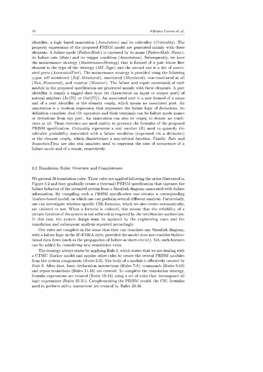
4.5 shows the transition matrix (left-hand side) and Markov model (right-hand side).
Again, this Markov chain corresponds exactly to the one recommended by ARP 4761.
The model presented in Figure 4.5 does not show any transitions associated to
multiple failure and repair transitions (from 0 to 3 and vice versa). This is because,
in the present con�guration, we do not have any common cause failure (simultaneous
failure) over the components. As long as the simultaneous occurrence of an event (that
is, b failure mode AND a failure mode happen in the same instant, where AND is
logical conjunction) was discarded in the quantitative analysis (because it could be
classi�ed as strongly unlikely, for instance), only the sequential occurrence of both
events (A then B or B then A) was considered by the tool.
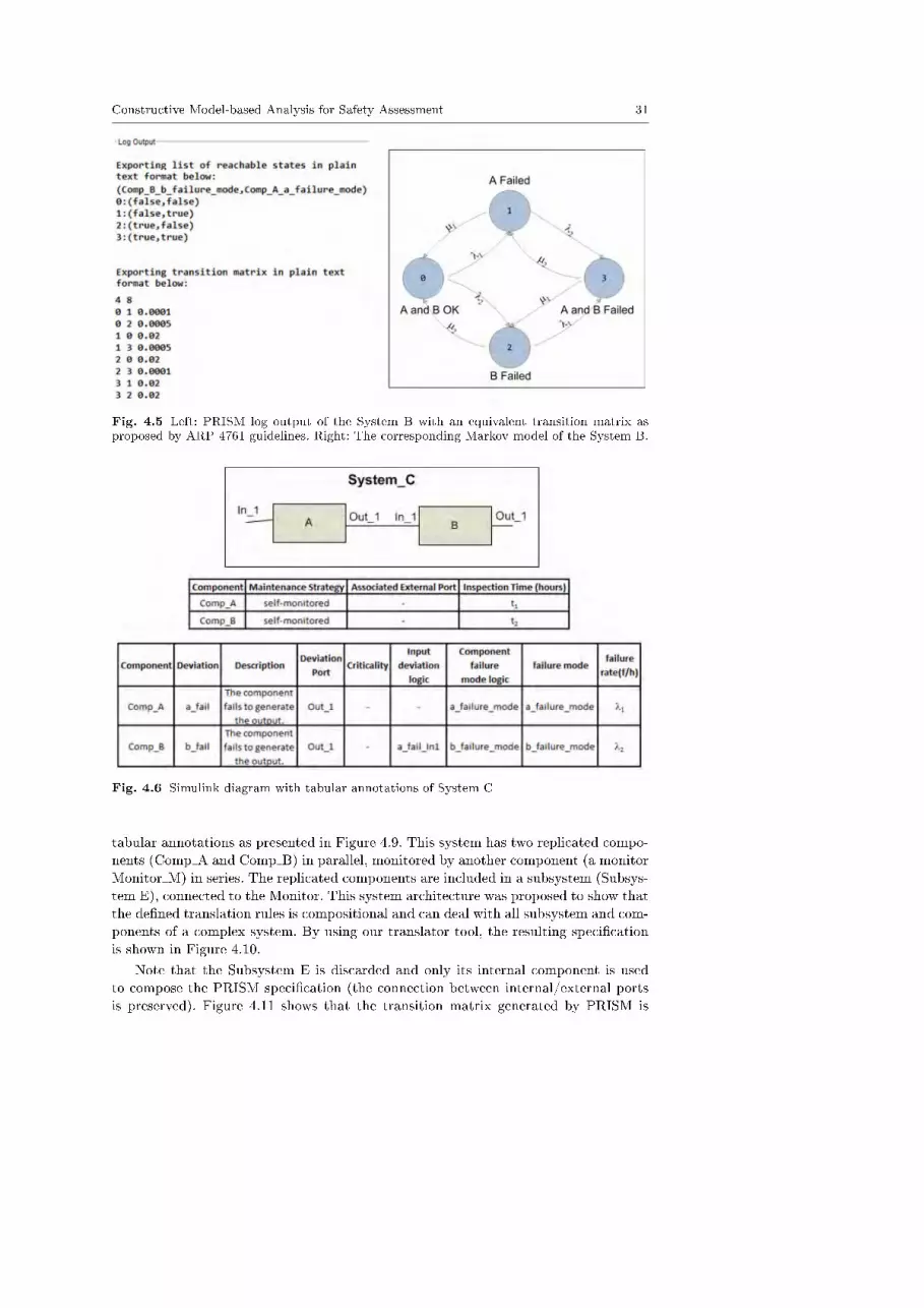
4.3 Third Case: Two Components in Series
In the next case, let System C be a system composed of two components (Comp A,
Comp B) in series and described in a Simulink diagram with tabular annotations as
presented in Figure 4.6. We also generate its PRISM speci�cation, S(C), by applying
our tool (see Figure 4.7). The resulting transition matrix and Markov model are shown
in Figure 4.8. By inspecting, we can obtain the same result as described by ARP 4761.
2 We assign real values for λ (0.0005) and 1/t (0.02) rates for PRISM to be able to compilethe generated speci�cation.

30 Adriano Gomes et al.
Fig. 4.3 Simulink diagram with tabular annotations of System B
ctmc
module Comp A
Comp A a failure mode : bool init false;
[]!(Comp A a failure mode)− > (1E − 4) : (Comp A a failure mode′ = true);
[](Comp A a failure mode)− > (1/50) : (Comp A a failure mode′ = false);
endmodule
formula A fail Comp A Out 1 = (Comp A a failuremode);
module Comp B
Comp B b failure mode : bool init false;
[]!(Comp B b failure mode)− > (5E − 4) : (Comp B b failure mode′ = true);
[](Comp B b failure mode)− > (1/50) : (Comp B b failure mode′ = false);
endmodule
formula B fail Comp B Out 1 = (Comp B b failure mode);
Fig. 4.4 PRISM speci�cation of System B
Note that this last generated model is similar to the previous one. As presented in ARP
4761, the di�erence between these two models is the failure states of each system. In
this case, the states 1 and 2 are also considered as failure states as well as state 3.
4.4 Fourth Case: Composed System
The last case considered corresponds to a system (System D) composed of three com-
ponents (Comp A, Comp B and Monitor M) described in a Simulink diagram with
Constructive Model-based Analysis for Safety Assessment 31
Fig. 4.5 Left: PRISM log output of the System B with an equivalent transition matrix asproposed by ARP 4761 guidelines. Right: The corresponding Markov model of the System B.
Fig. 4.6 Simulink diagram with tabular annotations of System C
tabular annotations as presented in Figure 4.9. This system has two replicated compo-
nents (Comp A and Comp B) in parallel, monitored by another component (a monitor
Monitor M) in series. The replicated components are included in a subsystem (Subsys-
tem E), connected to the Monitor. This system architecture was proposed to show that
the de�ned translation rules is compositional and can deal with all subsystem and com-
ponents of a complex system. By using our translator tool, the resulting speci�cation
is shown in Figure 4.10.
Note that the Subsystem E is discarded and only its internal component is used
to compose the PRISM speci�cation (the connection between internal/external ports
is preserved). Figure 4.11 shows that the transition matrix generated by PRISM is

32 Adriano Gomes et al.
ctmc
module Comp A
Comp A a failure mode : bool init false;
[]!(Comp A a failure mode)− > (1E − 4) : (Comp A a failure mode′ = true);
[](Comp A a failure mode)− > (1/50) : (Comp A a failure mode′ = false);
endmodule
formula A fail Comp A Out 1 = (Comp A a failuremode);
module Comp B
Comp B b failure mode : bool init false;
[]!(Comp B b failure mode)− > (5E − 4) : (Comp B b failure mode′ = true);
[](Comp B b failure mode)− > (1/50) : (Comp B b failure mode′ = false);
endmodule
formula B fail Comp B Out 1 = A fail Comp A Out 1 | (Comp Bb failure mode);
Fig. 4.7 PRISM speci�cation of System C
Fig. 4.8 Left: PRISM log output of the System C with an equivalent transition matrix asproposed by ARP 4761 guidelines. Right: The corresponding Markov model of the System C.
also equivalent to the transition matrix of the Markov model created by ARP 4761
guidelines. Furthermore, the generated transition matrix (Markov model) can assess
latent failure situations (monitor failure) as described in ARP 4671.
In summary, our strategy is sound with respect to the following assumptions:
� Component failures are detected in �ight only and repaired during ground main-
tenance or before the next �ight (description level), but the failures and repairs
occur at constant rates (model level);
� The system is assumed with perfect failure coverage and might recon�gure to a
degradable mode instantaneously.
In this paper we considered four patterns present in ARP 4671 to provide some valida-
tion for our rules. However, ARP 4671 includes other patterns that are simple variations
of the four patterns we have dealt with. In a way similar to that illustrated for the four
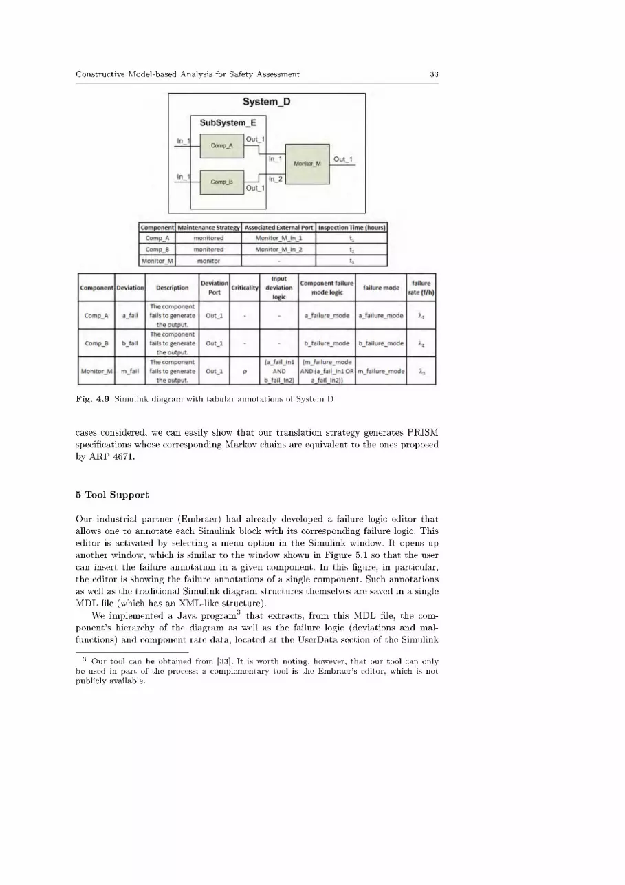
Constructive Model-based Analysis for Safety Assessment 33
Fig. 4.9 Simulink diagram with tabular annotations of System D
cases considered, we can easily show that our translation strategy generates PRISM
speci�cations whose corresponding Markov chains are equivalent to the ones proposed
by ARP 4671.
5 Tool Support
Our industrial partner (Embraer) had already developed a failure logic editor that
allows one to annotate each Simulink block with its corresponding failure logic. This
editor is activated by selecting a menu option in the Simulink window. It opens up
another window, which is similar to the window shown in Figure 5.1 so that the user
can insert the failure annotation in a given component. In this �gure, in particular,
the editor is showing the failure annotations of a single component. Such annotations
as well as the traditional Simulink diagram structures themselves are saved in a single
MDL �le (which has an XML-like structure).
We implemented a Java program3 that extracts, from this MDL �le, the com-
ponent's hierarchy of the diagram as well as the failure logic (deviations and mal-
functions) and component rate data, located at the UserData section of the Simulink
3 Our tool can be obtained from [33]. It is worth noting, however, that our tool can onlybe used in part of the process; a complementary tool is the Embraer's editor, which is notpublicly available.

34 Adriano Gomes et al.
ctmc
module Monitor M
Monitor M m failure mode : bool init false;
[](!Monitor M m failure mode)− > (1E − 4) : (Monitor M m failure mode′ = true);
[Monitor In1 Repair ](!Monitor M m failure mode)− >(1/100) : (Monitor M m failure mode′ = false);
[Monitor In1 DependentRepair ](Monitor M m failure mode)− >(1) : (Monitor M m failure mode′ = false);
[Monitor In2 Repair ](!Monitor M m failure mode)− >(1/500) : (Monitor M m failure mode′ = false);
[Monitor In2 DependentRepair ](Monitor M m failure mode)− >(1) : (Monitor M m failure mode′ = false);
endmodule
formula M fail Monitor Out 1 = (Monitor M m failure mode&
(A fail Comp A Out 1 | B fail Comp B Out 1)) |(A fail Comp A Out 1&B fail Comp B Out 1);
module Comp A
Comp A a failure mode : bool init false;
[]!(Comp A a failure mode)− > (1E − 4) : (Comp A a failure mode′ = true);
[Monitor In1 DependentRepair ](Comp A a failure mode)− >(1/50) : (Comp A a failure mode′ = false);
[Monitor In1 Repair ](Comp A a failure mode)− >(1) : (Comp A a failure mode′ = false);
endmodule
formula A fail Comp A Out 1 = (Comp A a failuremode);
module Comp B
Comp B b failure mode : bool init false;
[]!(Comp B b failure mode)− > (5E − 4) : (Comp B b failure mode′ = true);
[Monitor In2 DependentRepair ](Comp B b failure mode)− >(1/50) : (Comp B b failure mode′ = false);
[Monitor In2 Repair ](Comp B b failure mode)− >(1) : (Comp B b failure mode′ = false);
endmodule
formula B fail Comp B Out 1 = (Comp Bb failure mode);
Fig. 4.10 PRISM speci�cation of System D
MDL �le, and records in a tabular format as illustrated in Figure 5.2. According to
our rules, we need more information than that supplied by the failure editor, such as
maintenance strategy, criticality, etc. Therefore, currently, we have to manually com-
plement such an information, although the failure editor is being extended by Embraer
to allow the edition of the required additional information.
Besides implementing the extractor in Java, we created a Simulink parser to start
our translation, which is implemented in Java as well (see Figure 5.3). Thus, from the
user viewpoint, our translator is called by simply clicking the button Translate and
our translator performs the following steps:
1. It extracts all failure information generated using the failure editor;

Constructive Model-based Analysis for Safety Assessment 35
Fig. 4.11 Left: PRISM log output of the System D with an equivalent transition matrix asproposed by ARP guidelines. Right: The corresponding Markov model of the System D.
2. It extracts the structure (hierarchy) provided by the Simulink diagram (wired con-
nections);
3. It applies our rules as described in Figure 3.2;
4. It generates the PRISM speci�cation and its corresponding property expressions;
By activating the PRISM tool [36], it checks all criticality questions at once and iden-
ti�es the blocks where problems can be found. Currently, we are implementing an
Simulink plugin to performs all these step without leaving the Simulink environment.
In particular, an additional feature that, when a problem is found, will to send back the
violated criticalities to the failure editor, which will then highlight the corresponding
blocks. In this sense we substantially improve the safety assessment process Embraer
and other similar industrial safety assessment adopt, by avoiding generating a large
number of non-violating fault-trees. With our tool, a fault-tree is only built (for better
visualization of the problem) in the case of a safety violation. Eventually, when the
design is stable and no safety violation is reported, then a complete set of fault trees
can be created for certi�cation purposes; at Embraer, this is performed by a fault-tree
generation tool.
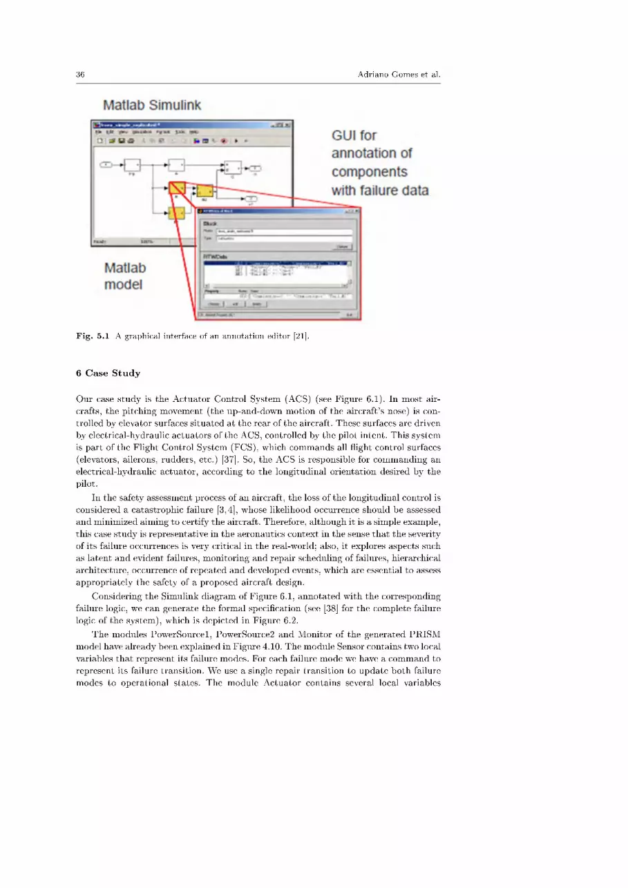
36 Adriano Gomes et al.
Fig. 5.1 A graphical interface of an annotation editor [21].
6 Case Study
Our case study is the Actuator Control System (ACS) (see Figure 6.1). In most air-
crafts, the pitching movement (the up-and-down motion of the aircraft's nose) is con-
trolled by elevator surfaces situated at the rear of the aircraft. These surfaces are driven
by electrical-hydraulic actuators of the ACS, controlled by the pilot intent. This system
is part of the Flight Control System (FCS), which commands all �ight control surfaces
(elevators, ailerons, rudders, etc.) [37]. So, the ACS is responsible for commanding an
electrical-hydraulic actuator, according to the longitudinal orientation desired by the
pilot.
In the safety assessment process of an aircraft, the loss of the longitudinal control is
considered a catastrophic failure [3,4], whose likelihood occurrence should be assessed
and minimized aiming to certify the aircraft. Therefore, although it is a simple example,
this case study is representative in the aeronautics context in the sense that the severity
of its failure occurrences is very critical in the real-world; also, it explores aspects such
as latent and evident failures, monitoring and repair scheduling of failures, hierarchical
architecture, occurrence of repeated and developed events, which are essential to assess
appropriately the safety of a proposed aircraft design.
Considering the Simulink diagram of Figure 6.1, annotated with the corresponding
failure logic, we can generate the formal speci�cation (see [38] for the complete failure
logic of the system), which is depicted in Figure 6.2.
The modules PowerSource1, PowerSource2 and Monitor of the generated PRISM
model have already been explained in Figure 4.10. The module Sensor contains two local
variables that represent its failure modes. For each failure mode we have a command to
represent its failure transition. We use a single repair transition to update both failure
modes to operational states. The module Actuator contains several local variables

Constructive Model-based Analysis for Safety Assessment 37
Fig. 5.2 Actuator Failure Logic Annotation
Fig. 5.3 Simulink to PRISM Tool
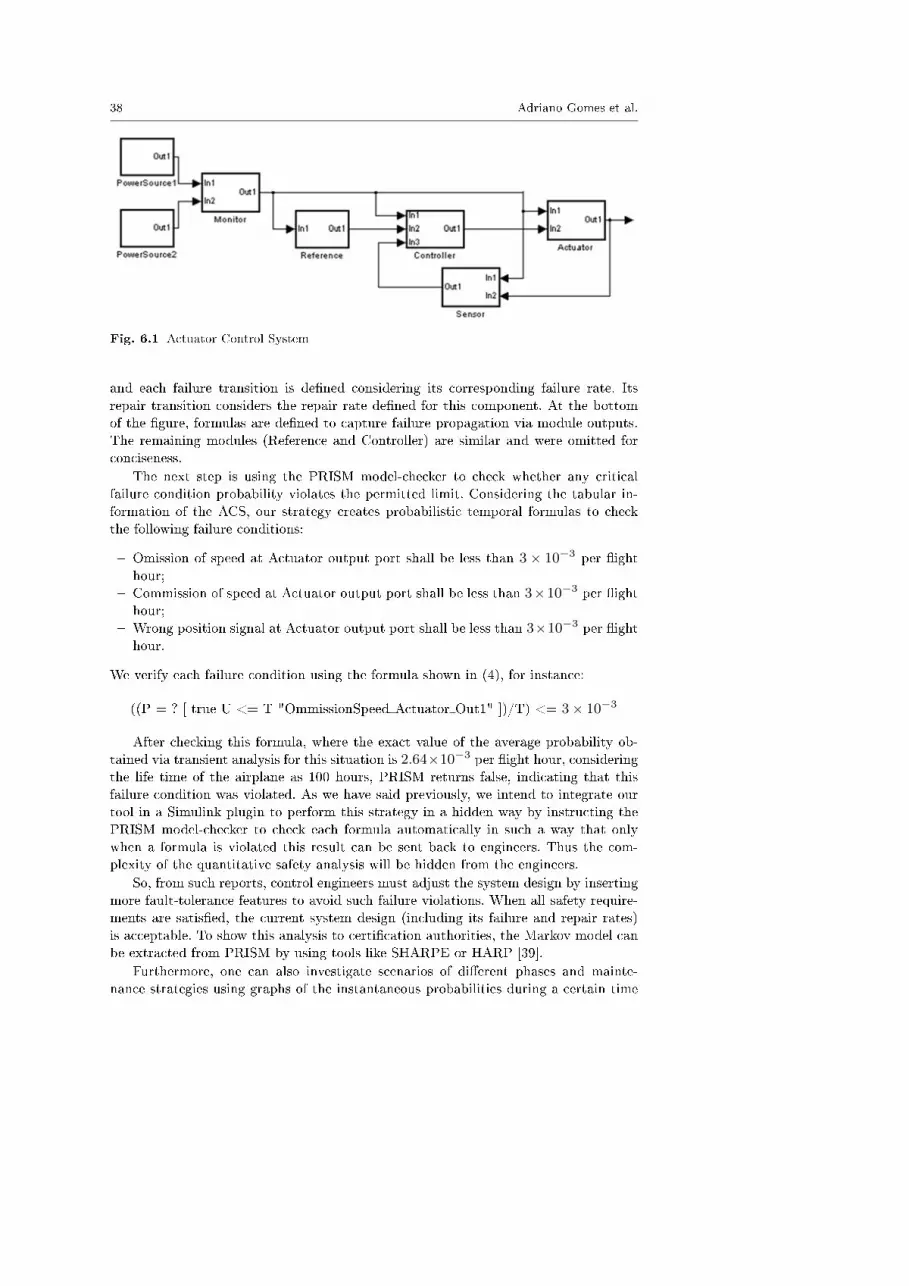
38 Adriano Gomes et al.
Fig. 6.1 Actuator Control System
and each failure transition is de�ned considering its corresponding failure rate. Its
repair transition considers the repair rate de�ned for this component. At the bottom
of the �gure, formulas are de�ned to capture failure propagation via module outputs.
The remaining modules (Reference and Controller) are similar and were omitted for
conciseness.
The next step is using the PRISM model-checker to check whether any critical
failure condition probability violates the permitted limit. Considering the tabular in-
formation of the ACS, our strategy creates probabilistic temporal formulas to check
the following failure conditions:
� Omission of speed at Actuator output port shall be less than 3 × 10⁻³ per �ight
hour;
� Commission of speed at Actuator output port shall be less than 3×10⁻³ per �ight
hour;
� Wrong position signal at Actuator output port shall be less than 3×10⁻³ per �ight
hour.
We verify each failure condition using the formula shown in (4), for instance:
((P = ? [ true U <= T "OmmissionSpeed Actuator Out1" ])/T) <= 3× 10⁻³
After checking this formula, where the exact value of the average probability ob-
tained via transient analysis for this situation is 2.64×10⁻³ per �ight hour, considering
the life time of the airplane as 100 hours, PRISM returns false, indicating that this
failure condition was violated. As we have said previously, we intend to integrate our
tool in a Simulink plugin to perform this strategy in a hidden way by instructing the
PRISM model-checker to check each formula automatically in such a way that only
when a formula is violated this result can be sent back to engineers. Thus the com-
plexity of the quantitative safety analysis will be hidden from the engineers.
So, from such reports, control engineers must adjust the system design by inserting
more fault-tolerance features to avoid such failure violations. When all safety require-
ments are satis�ed, the current system design (including its failure and repair rates)
is acceptable. To show this analysis to certi�cation authorities, the Markov model can
be extracted from PRISM by using tools like SHARPE or HARP [39].
Furthermore, one can also investigate scenarios of di�erent phases and mainte-
nance strategies using graphs of the instantaneous probabilities during a certain time

Constructive Model-based Analysis for Safety Assessment 39
ctmc
module PowerSource1 ... endmodule
module PowerSource2 ... endmodule
module Monitor ... endmodule
...
module Sensor
sensor sensorfailure : bool init false;
sensor sensordegradation : bool init false;
[](!sensor sensorfailure)− > (5E − 4) : (sensor sensorfailure′ = true);
[](!sensor sensordegradation)− > (5E − 4) : (sensor sensordegradation ′ = true);
[]((sensor sensorfailure | sensor sensordegradation))− > (1/5) :
(sensor sensorfailure′ = false)(sensor sensordegradation ′ = false);
endmodule
formula OmissionSignal Sensor Out1 = sensor sensorfailure |LowPower Monitor Out1 | OmissionSpeed Actuator Out1;
formula CorruptedSignal Sensor Out1 = sensor sensordegradation;
module Actuator
actuator lossofdriver : bool init false;
actuator lossofmotor : bool init false;
actuator mechanismjamming : bool init false;
actuator mechanismdegradation : bool init false;
actuator driverdegradation : bool init false;
[](!actuator lossofdriver)− > (1E − 4) : (actuator lossofdriver ′ = true);
[](!actuator lossofmotor)− > (1E − 3) : (actuator lossofmotor ′ = true);
[](!actuator mechanismjamming)− > (1E − 3) :
(actuator mechanismjamming ′ = true);
[](!actuator mechanismdegradation)− > (1E − 3) :
(actuator mechanismdegradation ′ = true);
[](!actuator driverdegradation)− > (1E − 5) : (actuator driverdegradation ′ = true);
[]((actuator lossofdriver | actuator lossofmotor | actuator mechanismjamming |actuator mechanismdegradation | actuator driverdegradation))− > (1/5) :
(actuator lossofdriver ′ = false)(actuator lossofmotor ′ = false)
(actuator mechanismjamming ′ = false)(actuator mechanismdegradation ′ = false)
(actuator driverdegradation ′ = false);
endmodule
formula OmissionSpeed Actuator Out1 = actuator lossofdriver | actuator lossofmotor
| actuator mechanismjamming | LowPower Monitor Out1 |OmissionSignal Component3 Out1;
formula WrongPosition Actuator Out1 = actuator mechanismdegradation |actuator driverdegradation | CorruptedSignal Component3 Out1;
formula CommissionSpeed Actuator Out1 = actuator driverdegradation |CommissionSignal Component3 Out1;
Fig. 6.2 Fragment of PRISM speci�cation

40 Adriano Gomes et al.
Fig. 6.3 Instantaneous probability during a period of time
interval. For instance, Figure 6.3 is the result of evaluating the following formula de-
�ned in (2), setting the T parameter from 0 to 100 hours. In Figure 6.3 the curves
for OmissionSpeed Actuator Out1 and WrongPosition Actuator Out1 basically colide
into one curve at the top part of the graph, since their values are very similar.
P=? [ true U<=T ("OmissionSpeed Actuator Out1") ]
P=? [ true U<=T ("CommissionSpeed Actuator Out1") ]
P =? [true U<=T ("WrongPosition Actuator Out1")]
With respect to this quantitative analysis, the main advantage is that the PRISM
models allow the creation and analysis of Markov chains in a more user-friendly and
condensed way. To give an idea of the probabilistic model checking e�ciency, the
e�ort to analyze the ACS design required 262,144 states and 3,989,504 transitions.
Nevertheless, only approximately 33.5 seconds and 7 MB of memory were necessary to
analyze each property expression of the system using PRISM version 3.3 beta 1 in an
Intel Core 2 Duo of 1.8 GHz, 2 GB RAM, HD 160 GB, Windows 7 Professional. It is
worth noting that PRISM supports models of more than 107 reachable states.
7 Related Work
A large amount of work has been done for quantitative safety assessment which is
based mainly on a previous qualitative analysis. An example of an e�ort in this di-
rection is the use of FTA to compute the failure conditions probability such as the
HAZOP [22] which evolves a design developed in Simulink; another relevant e�ort is
the ISAAC project where SCADE is used for modeling and safety analysis [15,14]. It is
also worth mentioning FSAP/NuSMV-SA [17], a fault injection approach developed in
the ESACS project. Due to the limitations of FTA methods, as discussed in Section 1,
more recently approaches considering dynamic reliability have been proposed, based
on timed-probabilistic models. We highlight four recent approaches.
In the COMPASS project [40], the model-based safety assessment is based on the
SLIM (System-Level Integrated Modeling) design language. The approach allows the

Constructive Model-based Analysis for Safety Assessment 41
extension of nominal model of the system adding probabilistic fault behavior (their
propagation and recovery, and degraded modes of operation), providing a precise char-
acterization of them based on a formal semantics. The analysis is based on a set of
veri�cation tools [17,8] (NuSMV, FSAP, RAT, Sigref, and MRMC) which allows ver-
ifying safety/dependability aspects and quantitative analyses (probabilistic analysis
of dynamic FTA). The completeness and consistency of this approach qualify it as a
promising solution, but the formal modeling language adopted is exposed to the user,
demanding that engineers be familiar with this notation. Thus, the impact for the
adoption of this solution might be signi�cant; our approach follows the hidden formal
methods view.
The work presented in [41] introducing quantitative reliability assessment into
Event- B modeling. Similarly to our work, Event-B is supported by a model-based plat-
form like Simulink (RODIN [42]) that provides a suitable framework for development
of systems as well as tool support for modeling and veri�cation (via theorem proving)
in the Event-B language. The work demonstrates how to integrate the stepwise system
development presented in Event-B modeling with probabilistic information to enable
quantitative veri�cation using the PRISM model checker, already at the development
stage. The work proposes a PRISM model of the system that allows combining logical
behavioral about the system functionalities with probabilistic reasoning about safety
by a model re�nement process. Although this work is also part of a framework solution-
oriented for industrial practice, the crucial step of the approach (the construction of
the PRISM model) is done manually (with a considerable e�ort, because the Event-B
model is not speci�ed in a compositional way). So the approach currently does not
enable an automatic translation of Event-B models to corresponding PRISM models,
possibly a�ecting its usability. Furthermore, the solution only deals with discrete time
models and focuses on modeling fail-safe systems, i.e., systems that shut down upon
occurrence of failure; thus, it does not deal with situations of repair components or
latent failures, for instance, limiting its applicability.
Another approach for automated model-based safety assessment is also presented
in one of the initiatives of the AVACS project [43]. The solution is based on a standard
design notation (Statecharts) supported by the industrial design tool Statemate. The
Statemate model is extended by fault injection and annotated with fault occurrence
distributions, generating an intermediate model (LTS) whose probabilities of reaching
a safety critical state is analyzed using the stochastic model checker MRMC [24]. A rel-
evant contribution is the ability to determine the particular Minimal Cut Sets from the
Markov event sequences (and thus identify those components), whose occurrence con-
tributes to reach a critical system failure state. Quantitative analysis can be performed
considering this reducted model (based on BDD and Stochastic Branching Bisimula-
tion [44]), in which only the actual possible failure sequences are taken into account.
However, this solution is limited to analyze only the critical permanent failures of a
system and also does not deal with situations of repair components or latent failures.
The work reported in [13] (which proposes pFMEA or Probabilistic FMEA) also
uses the PRISM model-checker to support quantitative analysis. The approach inte-
grates the failure behavior into the system model described in CTMC via failure injec-
tion. This work also uses the temporal languages (CSL, PCTL) to infer the probability
in which the failures can occur, considering the system particular failure modes. In one
sense, pFMEA performs a more detailed analysis than ours because it considers faulty
as well as nominal behaviors of a system. However, this approach does not generate
the model systematically and is more likely to generate state explosion, since it also

42 Adriano Gomes et al.
considers the nominal behavior of the system (values of each control variable) as well,
and thus the number of possible states of the system is potentially larger than ours.
8 Conclusion
In this paper we propose a systematic strategy to perform quantitative safety as-
sessment of critical systems. Our approach generates a PRISM speci�cation from a
Simulink diagram, annotated with failure logic. The strategy also creates CSL formu-
las that check whether safety requirements are satis�ed.
Systematically generating PRISM speci�cations seems a promising alternative to
explore because it allows the creation and analysis of Markov chains in a more user-
friendly and concise way. Our approach also eases the exploration of aspects such
as latent and evident failure, monitoring and repair schedule, which are essential to
aeronautical systems, for example.
This approach is not limited to just use Simulink diagrams as input. Actually, the
necessary input data, which contains information from the qualitative model and the
respective failure logic and propagation, is obtained from the tabular structures, which
are user de�ned. Simulink diagrams work implicitly with these structures [45,20]. Our
strategy follows a systematic process that has proved viable, since the tabular structures
are generated by traditional methods and analyses used by the aircraft industry during
the qualitative safety assessment (FHA, FMEA, IF-FMEA, CCA). So, con�guring our
implementation as a plug-in to some usual design tool, it is possible to e�ectively adopt
the proposed strategy in an industrial context.
Moreover, if we consider that the traditional fault-tree model is constructed to
assess the cause and probability of a single undesirable failure condition, the e�ort and
number of trees generated to perform the analysis of each failure condition is extremely
large, making the process expensive [3,20]. With Markov chains, for instance, those
created via PRISM, it is possible to represent all failure conditions of a system within
a single model. Also, checking the CSL formulas is less expensive than creating and
analyzing fault-trees. Furthermore, engineers can use the PRISM speci�cation (Markov
chains) to investigate dynamic aspects of a system: experiments to check existing failure
scenarios and phased mission can be performed by simply changing the values of local
variables of the model [3,10]. However, the current implementation of PRISM also
imposes some limitations.
We cannot generate counter-examples when some property is violated. Fortunately,
recent researches are already identifying counter-examples of stationary models, allow-
ing a better traceability of the basic failures and facilitating the cycle of checking and
validating the system design [46]; this is not available in PRISM yet. Other primary
limitation of a stochastic model checking is the size of the reachable state space, though
recent breakthroughs allow very large (> 107 reachable states) state spaces to be ex-
plored in reasonable time. To remedy this problem, hierarchical Markov models can
be used [47] but this needs an improvement in the way the probabilistic model checker
PRISM works because it must handle semi-markovian networks.
As future work we intend to incorporate the translation strategy as a complete
plug-in in the Matlab/Simulink software. Another improvement to this work is to con-
sider dynamic behavior for failure recovery, capturing the dynamic information in the
same way as the static information. We have addressed the relative completeness of
our translation, by presenting an overall scheme that summarizes a strategy for the

Constructive Model-based Analysis for Safety Assessment 43
application of each rule, based on a structural induction on the grammar presented in
Figure 3.1. Concerning soundness, currently our translation rules are able to generate
Markov models according to ARP 4761. Ideally, we plan to prove soundness using an
independent Markov semantics for Simulink. This would entail to establish an equiva-
lence between the Markov semantics of an arbitrary Simulink diagram and the Markov
model of the PRISM speci�cation generated via our translation. Finally, another di-
rection is to investigate some reduction techniques to overcome state explosion in the
context of PRISM. We intend to use abstraction strategies to reduce the Markov chains,
such as State Aggregation and Model Truncation, as well as compositional veri�cation.
Acknowledgements We would like to thank Diego Carvalho and Flávia Soares for theirhelp in developing the tool support. This work was partially supported by the National Insti-tute of Software Engineering (INES4), funded by CNPq and FACEPE, grants 573964/2008-4and APQ-1037-1.03/08, by CNPq grant 476821/2011-8 and by the Brazilian Space Agency(UniEspaço 2009).
References
1. D. Haasl, N. Roberts, W. Vesely, F. Goldberg, Fault tree handbook, Vol. 88 of Fault TreeHandbook, Systems and Reliability Research, O�ce of Nuclear Regulatory Research, U.S.Nuclear Regulatory Commission, 1981.
2. ARP4754, Certi�cation Considerations for Highly-Integrated or Complex Aircraft Sys-tems. Aerospace Recommended Practice (SAE International), Warrendale, PA (December1994).
3. ARP4761, Guidelines and Methods for Conducting the Safety Assessment Process on CivilAirborne Systems. Aerospace Recommended Practice (SAE International), Warrendale,PA (December 1996).
4. FAR25.1309, Federal Aviation Regulations FAR part 25.1309: System Design and Analysis.Advisory Circular (FAA, USA) (1977).
5. B. R. Haverkort, Markovian models for performance and dependability evaluation,Springer-Verlag New York, Inc., New York, NY, USA, 2002, pp. 38�83.
6. A. D. Dominguez-Garcia, J. G. Kassakianb, J. E. Schindallb, J. J. Zinchukc, An IntegratedMethodology for the Dynamic Performance and Reliability Evaluation of Fault-tolerantSystems, Reliability Engineering and System Safety 93 (2008) 1628�1649.
7. M. Bozzano, A. Villa�orita, The fsap/nusmv-sa safety analysis platform, Int. J. Softw.Tools Technol. Transf. 9 (2007) 5�24. doi:10.1007/s10009-006-0001-2.URL http://dl.acm.org:/citation.cfm?id=1229166.1229168
8. M. Bozzano, A. Cimatti, J.-P. Katoen, V. Nguyen, T. Noll, M. Roveri, The COMPASSApproach: Correctness, Modelling and Performability of Aerospace Systems, in: B. Buth,G. Rabe, T. Seyfarth (Eds.), Computer Safety, Reliability, and Security, Vol. 5775 ofLecture Notes in Computer Science, Springer Berlin / Heidelberg, 2009, pp. 173�186.URL http://dx.doi.org/10.1007/978-3-642-04468-7 15
9. A. Gomes, A. Mota, A. Sampaio, F. Ferri, J. Buzzi, Systematic model-based safety assess-ment via probabilistic model checking, in: Proceedings of the 4th international conferenceon Leveraging applications of formal methods, veri�cation, and validation - Volume PartI, ISoLA'10, Springer-Verlag, Berlin, Heidelberg, 2010, pp. 625�639.URL http://dl.acm.org/citation.cfm?id=1939281.1939338
10. M. Kwiatkowska, G. Norman, D. Parker, PRISM: Probabilistic Model Checking for Per-formance and Reliability Analysis, ACM SIGMETRICS Performance Evaluation Review36 (4) (2009) 40�45.
11. M. Kwiatkowska, G. Norman, D. Parker, PRISM 4.0: Veri�cation of Probabilistic Real-time Systems, in: G. Gopalakrishnan, S. Qadeer (Eds.), 23rd International Conference onComputer Aided Veri�cation (CAV'11), Vol. 6806, Springer, Snowbird, États-Unis, 2011,pp. 585�591.URL http://hal.inria.fr/hal-00648035
4 http://www.ines.org.br/
44 Adriano Gomes et al.
12. The MathWorks Inc., Simulink Validation and Veri�cation 2 User's Guide (2008).13. L. Grunske, R. Colvin, K. Winter, Probabilistic Model-Checking Sup-
port for FMEA, QEST '07: Proceedings of the Fourth InternationalConference on Quantitative Evaluation of Systems 0 (2007) 119�128.doi:http://doi.ieeecomputersociety.org/10.1109/QEST.2007.18.
14. A. Joshi, M. Heimdahl, Model-Based Safety Analysis of Simulink Models Using SCADEDesign Veri�er, in: R. Winther, B. Gran, G. Dahll (Eds.), Computer Safety, Reliability, andSecurity, Vol. 3688 of Lecture Notes in Computer Science, Springer Berlin / Heidelberg,2005, pp. 122�135.URL http://dx.doi.org/10.1007/11563228 10
15. Akerlund, O. et al, ISAAC, a framework for integrated safety analysis of functional, geo-metrical and human aspects, in: Proceedings of 3rd European Congress Embedded RealTime Software, ERTS 2006, Toulouse (France), 2006.
16. D. Harel, M. Politi, Modeling Reactive Systems with Statecharts: The Statemate Ap-proach, 1st Edition, McGraw-Hill, Inc., New York, NY, USA, 1998.
17. M. Bozzano, A. Villa�orita, Improving system reliability via model checking: TheFSAP/NuSMV-SA safety analysis platform, in: Proceedings of SAFECOMP 2003, LNCS2788, Edimburgh, Scotland, United Kingdom, Springer, 2003, pp. 49�62.
18. DO-178B, Software considerations in airborne systems and equipment certi�cation (RTCAInc.), Washington D.C. (December 1996).
19. Y. Papadopoulos, J. McDermid, R. Sasse, G. Heiner, Analysis and synthesis of the be-haviour of complex programmable electronic systems in conditions of failure, ReliabilityEngineering & System Safety 71 (3) (2001) 229�247.
20. O. Lisagor, J. McDermid, D. J. Pumfrey, Towards a practicable process for automatedsafety analysis, 24th International System Safety Conference (2006) 596�607.
21. Y. Papadopoulos, D. Parker, C. Grante, A method and tool support for model-based semi-automated failure modes and e�ects analysis of engineering designs, in: Proceedings of the9th Australian workshop on Safety critical systems and software - Volume 47, SCS '04,Australian Computer Society, Inc., Darlinghurst, Australia, Australia, 2004, pp. 89�95.URL http://dl.acm.org/citation.cfm?id=1082338.1082348
22. Y. Papadopoulos, M. Maruhn, Model-based synthesis of fault trees from matlab-simulink models, Dependable Systems and Networks, International Conference on (2001)0077doi:http://doi.ieeecomputersociety.org/10.1109/DSN.2001.941393.
23. C. Baier, B. R. Haverkort, H. Hermanns, J.-P. Katoen, Automated performance and de-pendability evaluation using model checking, in: Performance Evaluation of Complex Sys-tems: Techniques and Tools, Performance 2002, Tutorial Lectures, Springer-Verlag, Lon-don, UK, UK, 2002, pp. 261�289.URL http://dl.acm.org/citation.cfm?id=647414.725162
24. J.-P. Katoen, M. Khattri, I. S. Zapreev, A markov reward model checker, in: Proceedingsof the Second International Conference on the Quantitative Evaluation of Systems, IEEEComputer Society, Washington, DC, USA, 2005, pp. 243�. doi:10.1109/QEST.2005.2.
25. E. V. Sørensen, J. Nordahl, N. H. Hansen, From csp models to markov models, IEEETrans. Softw. Eng. 19 (6) (1993) 554�570. doi:10.1109/32.232021.URL http://dx.doi.org:/10.1109:/32.232021
26. A. Benveniste, E. Fabre, S. Haar, Markov nets: Probabilistic models for distributed andconcurrent systems, in: IEEE Transactions on Automatic Control, IEEE Computer Society,2003, pp. 1936�1950.
27. C. Baier, F. Ciesinski, G. Marcus, Probmela and veri�cation of markov decision processes,SIGMETRICS Perform. Eval. Rev. 32 (4) (2005) 22�27. doi:10.1145/1059816.1059821.URL http://doi.acm.org/10.1145/1059816.1059821
28. R. Alur, T. A. Henzinger, Reactive modules, Form. Methods Syst. Des. 15 (1) (1999) 7�48.doi:10.1023/A:1008739929481.URL http://dx.doi.org/10.1023/A:1008739929481
29. A. Aziz, K. Sanwal, V. Singhal, R. Brayton, Verifying continuous time markov chains,Springer, 1996, pp. 269�276.
30. M. Kwiatkowska, G. Norman, D. Parker, Quantitative analysis with the ProbabilisticModel Checker PRISM, Electronic Notes in Theoretical Computer Science 153 (2) (2009)5�31.
31. M. Kwiatkowska, G. Norman, D. Parker, Probabilistic symbolic model checking withPRISM: a hybrid approach, Int. J. Softw. Tools Technol. Transf. 6 (2) (2004) 128�142.doi:10.1007/s10009-004-0140-2.URL http://dx.doi.org/10.1007/s10009-004-0140-2

Constructive Model-based Analysis for Safety Assessment 45
32. C. A. R. Hoare, Communicating sequential processes, Commun. ACM 21 (8) (1978) 666�677. doi:10.1145/359576.359585.URL http://doi.acm.org/10.1145/359576.359585
33. Simulink to PRISM Tool.URL http://www.cin.ufpe.br/�acm/simulinktoprism/
34. Oxford University Computing Laboratory, The PRISM Language - Semantics (2004).URL http://www.prismmodelchecker.org/doc/semantics.pdf
35. W. Damm, M. Franzle, E. rudiger Olderog, A. Podelski, R. Wilhelm, M. Herbstritt,M. Herbstritt, R. Wimmer, T. Peikenkamp, E. Bode, M. Adelaide, S. Johr, H. Hermanns,B. Becker, Analysis of large safety-critical systems: A quantitative approach, in: Reportsof SFB/TR 14 AVACS 8, 2006.
36. Oxford University Computing Laboratory, Prism Model Checker (PRISM) (2004).URL http://www.prismmodelchecker.org/
37. J. B. J. Jesus, Designing and formal veri�cation of �y-by-wire �ight control systems,Master's thesis, Federal University of Pernambuco (2009).
38. A. J. O. Gomes, Model based Safety Analysis using Probabilistic Model Checking, Master'sthesis, Federal University of Pernambuco (2010).
39. D. Siewiorek, R. Swarz, Reliable Computer System: Design and Evaluation (3rd Ed), AK Peters/CRC Press, 1998.
40. M. Bozzano, A. Cimatti, J.-P. Katoen, V. Y. Nguyen, T. Noll, M. Roveri, Safety, depend-ability and performance analysis of extended aadl models, Comput. J. 54 (2011) 754�775.doi:http://dx.doi.org/10.1093/comjnl/bxq024.
41. A. Tarasyuk, E. Troubitsyna, L. Laibinis, Towards probabilistic modelling in event-b, in:Integrated Formal Methods - IFM 2010, Vol. 6396 of Lecture Notes in Computer Science,Springer Berlin / Heidelberg, Nancy, France, 2010, pp. 275�289.URL http://hal.inria.fr/inria-00524594/en/
42. The European Union ICT Project, Rigorous Open Development Environment for ComplexSystems (RODIN) (2008).URL http://www.event-b.org/
43. E. Bode, T. Peikenkamp, J. Rakow, S. Wischmeyer, Model based importance analysisfor minimal cut sets, in: Proceedings of the 6th International Symposium on AutomatedTechnology for Veri�cation and Analysis, Springer-Verlag, Berlin, Heidelberg, 2008, pp.303�317.
44. R. Wimmer, M. Herbstritt, H. Hermanns, K. Strampp, B. Becker, Sigref- a symbolicbisimulation tool box., in: ATVA 06, 2006, pp. 477�492.
45. A. Mota, J. Jesus, A. Gomes, F. Ferri, E. Watanabe, Evolving a safe system design itera-tively, in: Proceedings of the 29th international conference on Computer Safety, Reliability,and Security, Vol. 6351 of SAFECOMP'10, Springer-Verlag, Berlin, Heidelberg, 2010, pp.361�374.
46. H. Aljazzar, M. Fischer, L. Grunske, M. Kuntz, F. Leitner-Fischer, S. Leue, Safety Anal-ysis of an Airbag System Using Probabilistic FMEA and Probabilistic Counterexam-ples, Quantitative Evaluation of Systems, International Conference on 0 (2009) 299�308.doi:http://doi.ieeecomputersociety.org/10.1109/QEST.2009.8.
47. Y. Xie, S.-Z. Yu, A large-scale hidden semi-Markov model for anomaly detection on userbrowsing behaviors, IEEE/ACM Trans. Netw. 17 (2009) 54�65.


