1 2 3 4 5 6 7 8 9 10 11 12 13 14 15 16 17 18 19 20 21 22 23 24 25 26 27 28 29 30 31 32 33 34 35 36 37 38 39 40 41 42 43 44 45 46 47 48 49 50 51 52 53 54 55 56 57 58 59 60 61 62 63 64 65

1

Continuum Modeling of Micro-particle Electrorotation in Couette and

Poiseuille Flows—the Zero Spin Viscosity Limit

Hsin-Fu Huang a, b

, Markus Zahn *, b

, Elisabeth Lemaire c

a Department of Mechanical Engineering, Massachusetts Institute of Technology, Cambridge,

MA 02139, USA

b Laboratory for Electromagnetic and Electronic Systems, Research Laboratory of Electronics,

Department of Electrical Engineering and Computer Science, Massachusetts Institute of

Technology, Cambridge, MA 02139, USA

c Laboratoire de Physique de la Matière Condensée, CNRS-Université de Nice-Sophia Antipolis,

06108 Nice cedex 2, France

Abstract

A continuum mechanical model is presented to analyze the negative electrorheological responses

of a particle-liquid mixture with the suspended micro-particles undergoing Quincke rotation for

both Couette and Poiseuille flow geometries by combining particle electromechanics and

continuum anti-symmetric/couple stress analyses in the zero spin viscosity limit. We propose a

phenomenological polarization relaxation model to incorporate both the micro-particle rotation

speed and macro-continuum spin velocity effects on the fluid polarization during non-

equilibrium motion. Theoretical predictions of the Couette effective viscosity and Poiseuille flow

rate obtained from the present continuum treatment are in good agreement with the experimental

measurements reported in current literature.

Keywords: Electrohydrodynamics; Electrorotation; Quincke rotation; Negative electrorheological

effect; Continuum anti-symmetric/couple stress tensor

*Corresponding author: TEL: +1-617-253-4688; FAX: +1-617-258-6774; E-mail address:

zahn@mit.edu (Prof. M. Zahn)

ManuscriptClick here to view linked References

hal-0

0568

675,

ver

sion

1 -

23 F

eb 2

011

Author manuscript, published in "Journal of Electrostatics 68 (2010) 345-359"

1 2 3 4 5 6 7 8 9 10 11 12 13 14 15 16 17 18 19 20 21 22 23 24 25 26 27 28 29 30 31 32 33 34 35 36 37 38 39 40 41 42 43 44 45 46 47 48 49 50 51 52 53 54 55 56 57 58 59 60 61 62 63 64 65

2

1. Introduction

Electrorheological (ER) fluids are a class of fluids that consist of conducting or insulating

dielectric solid micro-particles suspended within a dielectric liquid medium. Due to the electrical

property (e.g., conductivity and/or permittivity) mismatch between the solid and liquid phases,

one can control the apparent macroscopic properties of the ER fluid such as the effective

viscosity for suspensions via the application of external direct current (DC) or alternating current

(AC) electric fields. Literature has therefore categorized ER effects, based on the flow or

rheological responses, into either positive ER or negative ER phenomena when the fluid

suspension is subjected to electric fields [1-6].

Upon the application of DC electric fields, Foulc et al. [4] discussed the important role of

electrical conductivities of the respective solid and liquid phases in determining the inter-particle

electrical force interactions in ER fluids. Boissy et al. [5] then further characterized and made

distinctions of macroscopic positive and negative ER responses based on different relative

magnitudes of the respective conductivities of the two phases. For ER fluids consisting of micro-

particles with a conductivity, 2 , larger than that, 1 , of the carrier liquid, stable particle chains

are formed in the direction of the electric field so that the macroscopic fluid resistance against

externally applied shear perpendicular to the electric field is enhanced and result in an increased

measured effective viscosity—the positive ER effect [1-3]. On the other hand, when the

conductivity of the carrier liquid is larger than that of the micro-particles, i.e., 1 2 , laminated

layers (perpendicular to the electric field) of packed particles resulting from electromigration are

formed adjacent to one of the two electrodes leaving a portion of the ER fluid relatively clear of

particles and hence leading to a reduction in the resistance against externally applied shear forces

perpendicular to the electric field; a decrease in the effective viscosity is measured—the negative

ER effect [5, 6].

Despite the relatively sparse reports on negative ER effects, recent experimental observations

found that: (i) with a given constant shear rate or equivalently the Couette boundary driving

velocity, the measured shear stress required to drive the Couette ER fluid flow is reduced (an

effectively decreased viscosity) and (ii) at a given constant pressure gradient, the Poiseuille flow

rate of the ER fluid can be increased both by applying a uniform DC electric field perpendicular

to the direction of the flows [7-12]. The mechanism responsible for the apparent increased flow

rate and decreased effective viscosity was attributed to the spontaneous electrorotation of the

hal-0

0568

675,

ver

sion

1 -

23 F

eb 2

011

1 2 3 4 5 6 7 8 9 10 11 12 13 14 15 16 17 18 19 20 21 22 23 24 25 26 27 28 29 30 31 32 33 34 35 36 37 38 39 40 41 42 43 44 45 46 47 48 49 50 51 52 53 54 55 56 57 58 59 60 61 62 63 64 65

3

dielectric micro-particles suspended within the carrier liquid, which is a mechanism different

from the traditional electromigration or particle electrophoresis explanation as mentioned in

previous negative ER literature [5, 6]. This spontaneous particle rotation under the action of a

DC electric field is often called “Quincke rotation” for G. Quincke‟s systematic study done in

1896 [13-18].

The origin of Quincke rotation can be illustrated by considering a dilute collection of

insulating dielectric spherical particles with permittivity 2 and conductivity 2 suspended in a

slightly conducting carrier liquid having a permittivity of 1 and a conductivity of 1 . The

material combination is chosen so that 2 1 where 1 1 1 and 2 2 2 are the charge

relaxation time constants of the liquid and the particles, respectively. When a uniform DC

electric field is applied across the dilute suspension, charge relaxation follows the Maxwell-

Wagner polarization at the solid-liquid interfaces, and each of the suspended particles attains a

final equilibrium dipole moment in the opposite direction to that of the applied DC field for the

condition of 2 1 . This, however, is an unstable equilibrium, and as the applied electric field

reaches a critical value [17, 18], namely,

0 12

1 1 2 2 1

81

2 3cE

, (1)

where 0 is the viscosity of the carrier liquid, the liquid viscous dampening can no longer

withstand any small perturbations misaligning the particle dipole moment and the applied DC

field. The electrical torque resulting from the misalignment exceeds the viscous torque exerted

on the micro-particle giving rise to spontaneous, self-sustained particle rotation either clockwise

or counter clockwise with the rotation axis perpendicular to the planes defined by the electric

field. When the particle-liquid suspension, or ER fluid, is driven by a boundary shear stress

(Couette flow) or a pressure gradient (Poiseuille flow), the macroscopic flow vorticity gives the

suspended micro-particles, instead of by random chance, preferable directions for rotation via

viscous interactions once the external electric field (generally larger than the critical field, cE ) is

applied. It is this combined effect of microscopic electrorotation and macroscopic flow vorticity

that gives rise to the newly observed negative ER phenomenon as described above [7-12].

Although models are given in current literature for analyzing the new phenomenon, they are

focused on the dynamics of a single particle and the utilization of a two-phase volume averaged,

hal-0

0568

675,

ver

sion

1 -

23 F

eb 2

011

1 2 3 4 5 6 7 8 9 10 11 12 13 14 15 16 17 18 19 20 21 22 23 24 25 26 27 28 29 30 31 32 33 34 35 36 37 38 39 40 41 42 43 44 45 46 47 48 49 50 51 52 53 54 55 56 57 58 59 60 61 62 63 64 65

4

effective medium description [7-12, 19]. Little has been done in developing a continuum

mechanical model from a more classical field theory based starting point in predicting the

dynamical behavior of fluids consisting of micro-particles undergoing spontaneous

electrorotation. To the best of the authors‟ knowledge, the ferrofluid spin-up flow is the most

representative flow phenomenon arising from internal particle rotation in current rheology

research [20-27].

In a ferrofluid spin-up flow, magnetic torque is introduced into the ferrofluid, which consists

of colloidally stabilized magnetic nanoparticles (typically magnetite) suspended in a non-

magnetizable liquid, through the misalignment of the particle‟s permanent magnetization and the

applied rotating magnetic field. The internal angular momentum of a continuum ferrofluid

„parcel‟ (containing a representative collection of liquid molecules and rotating magnetic

nanoparticles) becomes significant and the continuum stress tensor becomes anti-symmetric for

strong enough magnetic body torques introduced at the microscopic level. A moment-of-inertia

density is defined for the ferrofluid parcel based on the mass distributions of the liquid molecules

and magnetic particles in the parcel. A continuum spin velocity (column vector) is then defined

by the product of the internal angular momentum density (column vector) with the inverse of the

moment-of-inertia density (tensor) [28-30]. Since a ferrofluid continuum contains an enormous

amount of these parcels, the spin velocity, , is defined as a continuous field quantity which in

general, can be a function of space and time, i.e., , , ,x y z t . In order to describe how

microscopic particle rotation affects the continuum flow motion, a continuum angular

momentum conservation equation is added and coupled with the linear momentum equation so

that, in general, the externally applied magnetic body couple, angular momentum conversion

between linear and spin velocity fields, and the diffusive transport of angular momentum are

incorporated into the description of the flow momentum balances [22, 28-31].

A fundamental issue in the current development of ferrofluid spin-up flow is whether the

diffusive angular momentum transport or couple stress has a finite contribution to the angular

momentum balances of the flow. The current consensus is that the couple stress contribution is

vanishingly small, i.e., zero spin viscosity or diffusive transport conditions, as discussed in

Rosensweig [22], Chaves et al. [26, 27], and Schumacher et al. [32]. In a most recent work by

Feng et al. [33], scaling and numerical analyses were presented to show that in the limit of an

effective continuum, the angular momentum equation is to be couple stress free and the value of

hal-0

0568

675,

ver

sion

1 -

23 F

eb 2

011

1 2 3 4 5 6 7 8 9 10 11 12 13 14 15 16 17 18 19 20 21 22 23 24 25 26 27 28 29 30 31 32 33 34 35 36 37 38 39 40 41 42 43 44 45 46 47 48 49 50 51 52 53 54 55 56 57 58 59 60 61 62 63 64 65

5

the spin viscosity should be identically zero. However, spin-up velocity profiles measured by

ultrasound velocimetry reported by He [23], Elborai [24], and Chaves et al. [26, 27] were

compared with the numerical simulations of the full spin-up flow governing equations and found

that the experimental and numerical results would agree only if the spin viscosity assumes some

finite value instead of being vanishingly small or identically zero.

Acknowledging the experimental and theoretical discrepancies in the value of spin viscosity

and identifying the “mathematically analogous, physically parallel mechanisms” governing the

respective electrorotation and ferrofluid spin-up flows as summarized in Table 1, this work is

therefore aimed at developing a classical continuum mechanical model that combines particle

electrorotation and anti-symmetric/couple stress theories for describing the electrorheological

behavior of a particle-liquid mixture (termed ER fluid henceforward) subjected to a DC electric

field strength higher than the Quincke rotation threshold in both Couette and Poiseuille flow

geometries. Using a set of continuum modeling field equations similar to that utilized in

ferrofluid spin-up flow analyses, we investigate the effects of a zero spin viscosity, ' 0 , i.e.,

zero diffusive transport of angular momentum or couple stress free conditions, on the angular

momentum balances in the present negative ER fluid flow of interest. In the next section, the

governing equations describing the mass conservation, linear momentum conservation, angular

momentum conservation, and polarization relaxation of the ER fluid flow will be given in their

most general forms. The specific governing equations, analytical expressions of the spin velocity

solutions, and the evaluated numerical results are then presented, compared, and discussed in

Sections 3 and 4 to respectively show how the pertinent physical parameters are related to the ER

responses and fluid flow for two dimensional (2D) Couette and Poiseuille flows with internal

micro-particle electrorotation. A conclusion is given at the end of this article to summarize the

principle findings and the motivations for future research.

2. General Formulation

In order to quantitatively model and describe the present ER flow phenomenon, several

physical principles involved are considered: (i) the continuity or mass conservation, (ii) the linear

momentum balance, (iii) the angular momentum balance, and (iv) the polarization relaxation of

hal-0

0568

675,

ver

sion

1 -

23 F

eb 2

011

1 2 3 4 5 6 7 8 9 10 11 12 13 14 15 16 17 18 19 20 21 22 23 24 25 26 27 28 29 30 31 32 33 34 35 36 37 38 39 40 41 42 43 44 45 46 47 48 49 50 51 52 53 54 55 56 57 58 59 60 61 62 63 64 65

6

the ER fluid flow. The governing equations are given in the following subsections to describe the

above physical principles in proper mathematical forms.

2.1 The Fluid Mechanical Equations

The continuum equations describing the ER fluid motion are the mass continuity equation for

incompressible flow,

0v , (2)

the linear momentum equation,

22t e

Dvp P E v v

Dt , (3)

and the angular momentum equation,

22 2 ' 't

DI P E v

Dt

, (4)

where v is the linear flow velocity, is the ER fluid density, p is the hydrodynamic pressure

in the flow field, tP is the fluid total polarization, E is the electric field, is the flow spin

velocity, I is the average moment of inertia per unit volume, ' is the spin viscosity, is the

vortex viscosity which is related to the carrier liquid viscosity, 0 , and particle solid volume

fraction, , through 01.5 for dilute suspensions with 1 , is the sum of

the second coefficient of viscosity, , the zero field ER fluid viscosity, 0 1 2.5 , and the

negative of the vortex viscosity, e is the sum of the zero field ER fluid viscosity and the

vortex viscosity, ' ' ' is the sum of the spin viscosity and the second coefficient of spin

viscosity, ' [19, 22, 30], and D Dt is the material derivative given by

Dv

Dt t

. (5)

Note that Eq. (3) generally follows the form of the well known Navier-Stokes equation.

However, by introducing micro-particle rotation to the fluid flow, additional terms are included

in Eq. (3) to account for the Kelvin body force density, tP E , and the anti-symmetric force

density, 2 , as contributions in the linear momentum balances of the fluid flow. Moreover,

Eq. (4) characterizes the ER fluid parcel spin velocity, , so that the torque and angular

hal-0

0568

675,

ver

sion

1 -

23 F

eb 2

011

1 2 3 4 5 6 7 8 9 10 11 12 13 14 15 16 17 18 19 20 21 22 23 24 25 26 27 28 29 30 31 32 33 34 35 36 37 38 39 40 41 42 43 44 45 46 47 48 49 50 51 52 53 54 55 56 57 58 59 60 61 62 63 64 65

7

momentum balances resulting from the electrical torque input and fluid motion can be described

and related to other variables pertinent to this problem. In Eq. (4), the left hand side represents

the angular momentum per unit volume of a continuum ER fluid parcel; the first term on the

right hand side (RHS) represents the electrical torque density introduced to the flow field via the

rotating micro-particles under the action of the external DC field; the second term on the RHS

represents the angular momentum density transformation or conversion between the vorticity and

the spin velocity fields; the third term on the RHS represents the gradient of the divergence of

the spin velocity and is analogous to the “gradient of the divergence of the velocity” term in Eq.

(3) that measures the bulk compression effects in the fluid flow; and finally, the last term on the

RHS represents the diffusive transport of angular momentum within the flow field [22].

2.2 The Equilibrium Polarization and Polarization Relaxation Equations

The electric field in the ER flow field is generally described by the electro-quasi-static (EQS)

Maxwell equations [16, 34], namely,

0E , and (6)

0fD , (7)

where D is the electric displacement field and f is the free space charge density. Here, we

have assumed that on the macroscopic continuum level, the free space charge density is zero.

To complete the description of the electrical subsystem, we need a continuum

phenomenological polarization relaxation equation that accounts for the non-equilibrium effects

of both the linear and angular motions on the ER fluid polarization. Since the torque input on the

micro scale is related to the induced surface charge around the surface of the micro-particles, we

shall focus on how non-equilibrium motion, i.e., micro-particle rotation, , continuum fluid

spin velocity, , and continuum fluid velocity, v , affects the retarding polarization, P (the part

of polarization directly related to the surface charges [7-12]), instead of the total polarization of

the ER fluid, tP . Note that by definition, the spin velocity, , and the linear velocity, v , are

continuum variables which are related to respective averages of the internal angular momentum

and linear momentum over collections of micro-particles and carrier liquid molecules in an ER

fluid parcel. They should be distinguished from the micro-particle rotation velocity, , which is

the microscopic angular velocity of the suspended micro-particles within an ER fluid parcel.

hal-0

0568

675,

ver

sion

1 -

23 F

eb 2

011

1 2 3 4 5 6 7 8 9 10 11 12 13 14 15 16 17 18 19 20 21 22 23 24 25 26 27 28 29 30 31 32 33 34 35 36 37 38 39 40 41 42 43 44 45 46 47 48 49 50 51 52 53 54 55 56 57 58 59 60 61 62 63 64 65

8

We start the development of the polarization relaxation equation and its equilibrium

polarization from the micro scale. The governing equation for the two region problem of the

EQS fields within ( r R ) and outside ( r R ) a spherical solid particle suspended in a liquid

medium rotating at a constant speed, xi , subjected to a uniform electric field,

† †

0z z zE E i E i († denotes microscopic field quantities), as shown in Fig. 1 is the Laplace‟s

equation in spherical coordinates,

† † 2 †2 † 2

2 2 2 2 2

1 1 1sin 0

sin sinr

r r r r r

, (8)

where R is the radius of the micro-particle and † is the electric potential, i.e., † †E . The

boundary conditions on Eq. (8) are the electric field strength far away from the micro-particle,

†

0 0 cos sinz rE E i E i i as r , (9a)

the continuity of the electric potential at the solid-liquid interface,

† †, , , ,r R r R , (9b)

and charge conservation at the rotating micro-particle surface,

† † 0f fn J K at r R , (9c)

in which rn i is the normal vector of the spherical surface, † †

fJ E is the Ohmic current per

unit area, † † †

1 2, , , ,f r rn J E r R E r R with †

rE being the r component of

the electric field, I nn is the surface divergence, and †

f fK V is the surface

current density with † †

1 2, , , ,f r rE r R E r R and x rV i Ri R

sin cos cosi i . Using Eqs. (8) and (9), the electric potentials and electric fields within

and outside the rotating micro-particle can be solved by the method of separation of variables

with the aid of associated Legendre polynomials. This problem has been solved by Cebers [35];

here, we only summarize the solutions to the electric potential and the effective dipole moment

of the particle for r R . The outer electric potential ( r R ) is given in spherical coordinates as

hal-0

0568

675,

ver

sion

1 -

23 F

eb 2

011

1 2 3 4 5 6 7 8 9 10 11 12 13 14 15 16 17 18 19 20 21 22 23 24 25 26 27 28 29 30 31 32 33 34 35 36 37 38 39 40 41 42 43 44 45 46 47 48 49 50 51 52 53 54 55 56 57 58 59 60 61 62 63 64 65

9

†

13 62

1

†0 02

1

4cos sin sin

4, , cos cos

4t r a a

r

p ir rE rE

r

, (10)

where

2 1 2 1

1 2 1 23 2 13 0 2 2

1 2

2 2

2 1 MW

a E R

, (11)

2 1 2 1

1 2 1 236 0 2 2

2 2

1

MW

MW

a E R

, (12)

† † † †t x x y y z zp p i p i p i , (13)

sin cos sin sin cosr x y zi i i i , (14)

and

1 2

1 2

2

2MW

, (15)

is the Maxwell-Wagner relaxation time. With Eqs. (10)-(14), we can find the total dipole

moment of the rotating particle, †

tp , as † 0xp , †

1 64yp a , and †

1 34zp a , and the retarding

part of the dipole moment is then found as

† 3 2 11 6 1 3 0

1 224 4y za a E Rp i i

. (16)

The surface charge around the spherical particle with half of the hemisphere having positive

charge and the other half having negative charge is directly related to the retarding dipole

moment given by Eq. (16) [35]. By applying a torque balance between the electric torque,

† † † †

1 6 04t xp E p E a E i , and the viscous torque, 3

08 xR i , on the particle in steady

state, we can find the critical electric field for Quincke rotation as given in Eq. (1) and the

rotation velocity of the micro-particle being [18]

hal-0

0568

675,

ver

sion

1 -

23 F

eb 2

011

1 2 3 4 5 6 7 8 9 10 11 12 13 14 15 16 17 18 19 20 21 22 23 24 25 26 27 28 29 30 31 32 33 34 35 36 37 38 39 40 41 42 43 44 45 46 47 48 49 50 51 52 53 54 55 56 57 58 59 60 61 62 63 64 65

10

0

0

2

0 ,

0,

11 c

c

cMW

E E

E E

E

E

, (17)

where the + and - signs denote counter clockwise and clockwise rotation with the coordinate

system defined in Fig. 1. In Eq. (17), we have assumed that the particle rotation is only in the x-

direction; this is because we will only be considering 2D flow geometries in the following

discussions. Note however that for the most general cases, the particle rotation axis is

perpendicular to the planes defined by the electric field, which has a three dimensional feature.

We next consider a dilute particle suspension with a solid volume fraction of and a particle

number density of n subjected to the DC electric field. The solid volume fraction and the

particle number density are related through

3

3

6

dn O nR

, (18)

where 2d R is the diameter of the micro-particle. Assuming that the mutual electrical

interactions between the suspended micro-particles can be neglected (i.e., dilute suspension with

1 ), the macroscopic retarding polarization of the ER fluid at equilibrium, eqP , can be

obtained by multiplying Eq. (16) with the particle number density, n , i.e., †

eqP np

y z

eq y eq zP i P i , with

0

2 1 2 1

1 2 1 2

2 2

31

2 1 2 1

1 2 1 2

2 2

2 2

1

2 2

1

4

MW

yMWeq

zeq

MW

EP

nRP

. (19)

Equation (19) represents the macroscopic retarding polarization of a static, motionless ER fluid,

namely, 0 and 0v . However, this does not mean that at macroscopic equilibrium, the

micro-particles cannot rotate on the microscopic level, i.e.. 0 , when the applied electric field

is larger than the critical electric field given in Eq. (1), that is, 0 cE E . This formulation is

similar to the dynamic effective medium model shown by Xiao et al. [36]. As for the cases of

hal-0

0568

675,

ver

sion

1 -

23 F

eb 2

011

1 2 3 4 5 6 7 8 9 10 11 12 13 14 15 16 17 18 19 20 21 22 23 24 25 26 27 28 29 30 31 32 33 34 35 36 37 38 39 40 41 42 43 44 45 46 47 48 49 50 51 52 53 54 55 56 57 58 59 60 61 62 63 64 65

11

0 cE E , is set to zero in Eq. (19) since an applied field less than the critical field will give

imaginary values of and the real root can only be zero as in Eq. (17). Note that by setting the

micro-particle rotation speed to zero, the equilibrium retarding polarization shown in Eq. (19)

reduces back to the one given by Cebers [35], i.e., all micro-particle rotation speed, continuum

linear velocity, and continuum spin velocity equal to zero. Combining Eqs. (17) and (19) and

extending the physical arguments of the phenomenological magnetization relaxation equation

proposed by Shliomis [22, 37, 38] to the case of the retarding polarization, we arrive at the

following retarding polarization relaxation equation,

1eq

MW

DPP P P

Dt

, (20)

where P is the retarding polarization.

Equations (17), (19), and (20) account for the non-equilibrium effects of the micro-particle

rotation velocity, , ER fluid spin velocity, , and ER fluid linear velocity, v , on the retarding

polarization. In the development of Eqs. (17), (19), and (20), we have assumed that the induced

dipole moment on the micro-particles obeys the Maxwell-Wagner polarization—the induced

charges are distributed on the surface of the particles at the micro scale. We have also assumed

that only the retarding part of the macroscopic ER fluid polarization, i.e., the polarization directly

related to the interfacial charges, needs to be relaxed according to the non-equilibrium motions.

Unlike the ferrofluid equilibrium magnetization, the equilibrium retarding polarization, Eq. (19),

does not follow a Langevin function [22]. This is because we are considering the rotation of

micro-sized dielectric insulating particles on which Brownian motion has little influence [18].

Rigorously speaking, the micro-particle rotation speed, , that enters Eqs. (19) and (20) should

be the speed observed in the reference frame that rotates with the ER fluid parcel. Yet, the

mathematical analysis of this ER fluid flow will become much more involved and impractical in

attempts to correct for the difference in reference frames, and is beyond the scope of this work.

As a first approach, we employ Eq. (17) in Eqs. (19) and (20) to incorporate both microscopic

(i.e., ) and macroscopic (i.e., and v ) motions under one continuum mechanical framework.

hal-0

0568

675,

ver

sion

1 -

23 F

eb 2

011

1 2 3 4 5 6 7 8 9 10 11 12 13 14 15 16 17 18 19 20 21 22 23 24 25 26 27 28 29 30 31 32 33 34 35 36 37 38 39 40 41 42 43 44 45 46 47 48 49 50 51 52 53 54 55 56 57 58 59 60 61 62 63 64 65

12

3. Couette Flow with Internal Micro-particle Electrorotation

3.1 The Governing Equations Specific to the Couette Flow Geometry

Consider the Couette flow geometry shown in the schematic diagram of Fig. 2. The lower

plate of the parallel plate system is fixed at zero velocity while the upper plate is applied with a

constant velocity, 0U , in the positive y-direction. We assume that the flow is steady ( 0t ),

incompressible, fully developed ( 0y ), and two-dimensional ( 0x ) in Cartesian

coordinates. Under these assumptions, the continuity equation, Eq. (2), with y y z zv u i u i is

readily reduced to 0zdu dz and subsequently to 0zu since the z-velocity component, zu ,

has to satisfy the no-slip and non-penetrating (impermeable walls) boundary conditions at 0z

and h with h being the height of the 2D channel. Moreover, by using the EQS Faraday‟s

equation, Eq. (6), with y y z zE E i E i and the condition of fully developed flow, we find

0ydE dz such that yE is just a constant throughout the 2D channel. Noting that the

boundaries at 0z and h are perfectly conducting electrodes, and that the tangential component

of the electric field is continuous across the boundaries, the constant yE is simply zero.

Therefore, the applied DC electric field is to be in the z-direction only. The fringing effects at the

ends of the channel are to be neglected.

The governing equations are further simplified by considering a zero spin viscosity, i.e.,

' 0 , in the angular momentum equation, Eq. (4). Given the above assumptions combined with

the continuity and zero spin viscosity conditions, Eqs. (3), (4), and (20), are then simplified into

the following:

0y

MW x z y eqP P P , (21a)

0z

MW x y z eqP P P , (21b)

2

22 0

yxe

d ud

dz dz

, (22)

and

2 2 0y

y z x

duP E

dz

, (23)

where yu is the y-velocity component, x is the x-spin velocity component (note: x xi in

hal-0

0568

675,

ver

sion

1 -

23 F

eb 2

011

1 2 3 4 5 6 7 8 9 10 11 12 13 14 15 16 17 18 19 20 21 22 23 24 25 26 27 28 29 30 31 32 33 34 35 36 37 38 39 40 41 42 43 44 45 46 47 48 49 50 51 52 53 54 55 56 57 58 59 60 61 62 63 64 65

13

2D), zE is the z-component of the applied DC electric field, and yP and zP are respectively the

retarding polarization components in the y- and z- directions, i.e., y y z zP P i P i . Note that we

have substituted the total polarization, tyP , with the retarding polarization, yP , in Eq. (23). This

is because the DC electric field is applied in the z-direction only with 0yE . Thus the total

polarization in the y-direction comes from the dipole moment tilt of the rotating micro-particles

in the micro scale, which, on the macroscopic level, is generally the y-component of the retarding

polarization. Finally, the z-linear momentum equation reduces to an equation which relates only

the pressure gradient to the Kelvin body force density, and thus can be treated separately from

the other equations.

Substituting Eq. (19) into Eq. (21), we can solve for the y- and z- components of the retarding

polarization as

02 21

y x zMW

y

xMW

P n E

, (24a)

02 21

z x yMW

z

xMW

P n E

, (24b)

where

2 1 2 1

1 2 1 2

2 1 2 1

1 2 1 2

2 23

1

2 2

2 2

2 2

14

1

MW

y MW

z

MW

R

, (25)

with given in Eq. (17). Generally speaking, the z-component of the electric field, zE , in Eq.

(23) depends on the flow linear and spin velocities, and the EQS equations, Eqs. (6) and (7),

need to be solved together with the retarding polarization, Eqs. (24) and (25), linear momentum,

Eq. (22), and angular momentum, Eq. (23), equations with the suitable electrical and mechanical

boundary conditions applied at 0z and h . However, the coupled set of governing equations

becomes much more non-linear and less practical for engineering analysis purposes. Assuming

that, due to flow motion, corrections to the z-electric field, zE , can be related to the microscopic

applied electric field and the micro-particle solid volume fraction through

hal-0

0568

675,

ver

sion

1 -

23 F

eb 2

011

1 2 3 4 5 6 7 8 9 10 11 12 13 14 15 16 17 18 19 20 21 22 23 24 25 26 27 28 29 30 31 32 33 34 35 36 37 38 39 40 41 42 43 44 45 46 47 48 49 50 51 52 53 54 55 56 57 58 59 60 61 62 63 64 65

14

† 2 2

1 2 0 1 2z zE E e e E e e , (26)

where ie ‟s are the correction terms, we substitute Eq. (24a) into Eq. (23) and approximate to the

first order of magnitude of the volume fraction, , 0 1zE E e for dilute suspensions, i.e.,

1 , so that the electrical field equations, Eqs. (6) and (7), can be decoupled from the

mechanical field equations, Eqs. (2)-(4), or Eqs. (22) and (23). Hence the governing equations

specific to the Couette flow geometry with internal particle electrorotation is obtained as Eq. (22)

and

*2

02 22 2 0

1

yMW xz x

MW x

dun E

dz

. (27)

where *

y z MW . In Eq. (27), the first order correction, 1e , to the z-electric field has

been neglected because 1e has become a second order term after being substituted into Eq. (23),

i.e., 0 0 0 1z z zn E E n E E e with 1 and 3 3

zn nR nd O as in Eq. (18).

The boundary condition for the velocity field, yv u yi , is the general no-slip boundary

condition, i.e., 0v at 0z and 0v U yi at z h . On the other hand, the angular momentum

equation, Eq. (27), eventually reduces to an algebraic equation for zero spin viscosity conditions

as will be discussed shortly in Section 3.2; hence, there are no additional constraints to be

applied at the boundaries for the Couette spin velocity field. This “free-to-spin” condition on x

for ' 0 is likely an analogous case to the Euler equation for inviscid fluid flow—the linear

flow velocity is allowed to slip at the solid-fluid boundaries when the fluid viscosity goes to

zero.

3.2 Solutions to the Spin Velocity and Effective Viscosity

Integrating Eq. (22) with respect to z, we have

2y

x e c

duC

dz , (28)

where cC is a constant. Substituting Eq. (28) into Eq. (27), we find that the spin velocity, x ,

does not depend on the spatial coordinate, z, and therefore Eq. (22) reduces to the original

governing equation for simple Couette flow, i.e.,

hal-0

0568

675,

ver

sion

1 -

23 F

eb 2

011

1 2 3 4 5 6 7 8 9 10 11 12 13 14 15 16 17 18 19 20 21 22 23 24 25 26 27 28 29 30 31 32 33 34 35 36 37 38 39 40 41 42 43 44 45 46 47 48 49 50 51 52 53 54 55 56 57 58 59 60 61 62 63 64 65

15

2

20

yd u

dz , (29)

and the solution to Eq. (29) is

0y

Uu z z

h . (30)

Inserting Eq. (30) into Eq. (27) and using the following non-dimensionalization scheme, namely,

*xMW , * 0

MW

U

h , and *

2

0

2

z MW

Mn E

, (31)

the non-dimensional angular momentum equation is obtained as

* * **3 *2 *

* *

11 0

2 2 2 2M M

. (32)

Equation (32) can be solved to obtain analytical expressions by symbolic calculation

packages (Mathematica, Wolfram Research, Inc.) and the three roots of Eq. (32) are expressed as

functions of * and *M . Nevertheless, it should be pointed out that not all the three roots to *

are likely to be physically meaningful and interpretable for the flow phenomena of interest

presented herein. Moreover, each of the three roots may vary from real to complex valued (or

vice versa) in different parametric regimes. In order to find the most physically meaningful and

interpretable solution or combination of solutions from the three possible roots to the current

problem, the following considerations and conditions are applied to the flow field: (i) only real

valued solutions are considered, (ii) the ER fluid is “free-to-spin” at the solid-ER fluid

boundaries since the governing physics reduce from a boundary value problem to an algebraic

problem in zero spin viscosity conditions, and (iii) due to micro scale viscous interactions, the

micro-particle angular velocity, , should rotate in the same direction as that of the macroscopic

ER flow vorticity so that the micro-particle rotation is always stable [7-12].

We have shown that the spin velocity is a constant throughout the channel when ' 0 in the

Couette geometry. Hence, * assumes some finite value at the solid-ER fluid boundaries, which

is readily self-consistent with the “free-to-spin” condition. To satisfy condition (iii) for 0 cE E ,

we need to substitute into Eqs. (24) and (25) the micro-particle angular velocity with the minus

sign in Eq. (17) which has the same negative sign (or clockwise rotation) as the macroscale

Couette flow vorticity, namely, y xv du dz i 0 xU h i , with the coordinate systems

hal-0

0568

675,

ver

sion

1 -

23 F

eb 2

011

1 2 3 4 5 6 7 8 9 10 11 12 13 14 15 16 17 18 19 20 21 22 23 24 25 26 27 28 29 30 31 32 33 34 35 36 37 38 39 40 41 42 43 44 45 46 47 48 49 50 51 52 53 54 55 56 57 58 59 60 61 62 63 64 65

16

defined in Figs. 1 and 2. For 0 cE E , we employ 0 (see Eq. (17)) in Eqs. (24) and (25) and

pick out or select the root to the spin velocity, * or x , that has the same negative sign as the

Couette flow vorticity. For the parametric regimes of our interests, we identify the stable and real

valued solution to the spin velocity as: for 0 cE E (use negative value in Eqs. (17), (24), and

(25)),

1

1 1*3 3* * 3 2 3 23

2 1 2 1 2 2 1 2*3

11 3 6 4 4 1 3 4

6 12 2C C C C C C C Ci M i

M

, (33)

for 0 0.8 cE E (use 0 in Eqs. (17), (24), and (25)),

1

1 1*3 3* * 3 2 3 23

1 1 2 1 2 2 1 2*3

13 4 4 4

6 6 2C C C C C C C CM

M

, (34)

and for 00.8 c cE E E with 0 in Eqs. (17), (24), and (25), * is given by both *

1C and

*

2C , i.e., Eqs. (33) and (34), where

* *2 *2 *2

1 6 12C M M M , (35)

and

*2 * *3 * *3 *3 *2 *

2 18 72 2 108C M M M M . (36)

Note that the results shown in Eqs. (33)-(36) are obtained under the “Solve” command of

Mathematica. In 00.8 c cE E E , part of the real valued solution to * is given by Eq. (33) and

the other part is given by Eq. (34), thus, both solutions have to be used in the evaluation of the

spin velocity solutions.

The effective viscosity of Couette flows with particle electrorotation, eff , is derived by

recognizing the relationship between the wall shear stress, s , and the average shear rate (or the

velocity of the upper plate, 0U , divided by the channel height, h ) when the shear stress is held

constant for a given flow or experimental condition, i.e.,

*

0s eff eff z y

MW

Ui T i

h

, (37a)

in which denotes the shear stress differences across the solid-liquid interface, zi is the row

hal-0

0568

675,

ver

sion

1 -

23 F

eb 2

011

1 2 3 4 5 6 7 8 9 10 11 12 13 14 15 16 17 18 19 20 21 22 23 24 25 26 27 28 29 30 31 32 33 34 35 36 37 38 39 40 41 42 43 44 45 46 47 48 49 50 51 52 53 54 55 56 57 58 59 60 61 62 63 64 65

17

vector 0 0 1 , yi is the column vector 0 1 0

t, and

s aT T T is the total stress tensor

with the symmetric part being

0 0

0

0

ty

s

y

p

duT pI v v p

dz

dup

dz

, (37b)

and the anti-symmetric part being

0 0 0

2 0 0 2

0 2 0

y

a x

y

x

duT v

dz

du

dz

, (37c)

[22]. By expanding the total stress tensor into matrix form as in Eqs. (37b) and (37c) and

substituting the velocity field, Eq. (30), and the spin velocity field, Eq. (33) and/or (34), into Eq.

(37), the effective viscosity defined in Eq. (37a) can be obtained as

*

*2eff e

, (38a)

or in dimensionless terms,

**

*

2eff e Ci

, (38b)

where * *

1Ci C and/or *

2C depending on the regimes of the electric field strength where *

Ci

become real valued, and 0 1 2.5 is the zero field ER fluid (particle-liquid mixture)

viscosity as defined in Section 2.1. The shear stress difference in Eq. (37a) is evaluated at 0z .

3.3 Results and Discussions

After obtaining the velocity and spin velocity fields as well as the effective viscosity, we now

further present the numerical evaluations of the analytical expressions given in Eqs. (33), (34),

and (38). The system parameters, physical constants, and material properties used in our

hal-0

0568

675,

ver

sion

1 -

23 F

eb 2

011

1 2 3 4 5 6 7 8 9 10 11 12 13 14 15 16 17 18 19 20 21 22 23 24 25 26 27 28 29 30 31 32 33 34 35 36 37 38 39 40 41 42 43 44 45 46 47 48 49 50 51 52 53 54 55 56 57 58 59 60 61 62 63 64 65

18

evaluations follow those given in Ref. [7-12] so as to facilitate a more effective comparison

between the current continuum model and the two-phase effective continuum formulation found

in the literature. These data are summarized in Table 2.

Shown in Fig. 3 is the Couette spin velocity, *

MW x , given by Eq. (33), i.e., * *

2C ,

for 0 cE E and by Eq. (34), i.e., * *

1C , for 0 0.8 cE E plotted with respect to the average

shear rate, *

0MWU h , evaluated at *

0 cE E E 0, 0.4, 0.8, 1.0, 2.0, and 3.0 where

61.3 10cE (V m ) is the critical electric field for the onset of particle Quincke rotation

evaluated by Eq. (1). It is learned from Fig. 3 that the magnitude of the spin velocity within the

flow field increases as the applied electric field strength is increased with * kept constant. On

the other hand, the ER fluid spin magnitude also increases as the average shear rate, * , or the

applied velocity of the upper boundary, 0U , increases while the electric field strength is kept

constant. As the applied electric field, 0E or *E , is gradually reduced, the ER fluid spin velocity

gradually reduces back to the zero electric field angular velocity of a continuum fluid parcel, i.e.,

* *

0 2 , or half of the Couette flow vorticity, which can be readily deduced from Eq. (32)

by letting *M or 0 0E . This solution is noted by the top most, gray line with * 0E in

Fig. 3.

Notice that for a given field strength and shear rate, the spin velocity, * or x , is a constant

throughout the channel and, thus, does not depend on the spatial z-coordinate as already

discussed in Section 3.2 for the Couette geometry. With the spin velocity being a constant in Eq.

(22), the velocity field of Couette flow with internal micro-particle electrorotation is found to be

the same as that of Couette flow without particles—a result consistent with those given in

Shliomis [39] and Rosensweig [22]. Thus, the velocity field of Couette flow with micro-particle

electrorotation in the zero spin viscosity limit is simply the linear profile given by Eq. (30).

Figure 4 shows the effective viscosity, *

eff , of Couette flow with internal micro-

particle electrorotation as given in Eq. (38). The effective viscosity is plotted with respect to the

average shear rate, * , with the electric field strength being evaluated at *E 0, 0.4, 0.8, 1.0,

2.0, and 3.0. Again, the spin velocity solution given by Eq. (33) is employed in Eq. (38) for

conditions of *

0 1cE E E , whereas Eq. (34) is employed in Eq. (38) for * 0.8E . It is readily

hal-0

0568

675,

ver

sion

1 -

23 F

eb 2

011

1 2 3 4 5 6 7 8 9 10 11 12 13 14 15 16 17 18 19 20 21 22 23 24 25 26 27 28 29 30 31 32 33 34 35 36 37 38 39 40 41 42 43 44 45 46 47 48 49 50 51 52 53 54 55 56 57 58 59 60 61 62 63 64 65

19

seen that the effective viscosity decreases as the applied DC electric field strength increases.

However, as the magnitude of the shear rate increases, the amount of reduction in the effective

viscosity decreases regardless of the applied electric field strength. Since the effective viscosity

is normalized and non-dimensionalized by the zero electric field ER fluid viscosity, , we

further point out that the value of * should approach one as the applied electric field goes to

zero, which is a result easily found by substituting * *

0 2 into Eq. (38). The zero electric

field result is indicated by the gray line in Fig. 4. It can be seen from the figure that the predicted

effective viscosities * approach to one when the shear rate, * , goes large or when the applied

electric field strength is reduced.

From Fig. 4, we find that zero or negative viscosities are attainable when the applied DC

electric field strength is strong enough. By using the terms “zero or negative viscosities,” we do

not mean that the true fluid viscosity is zero or negative, but that the effective or apparent

viscosity comes out to be zero or a negative value through performing the force balance

described by Eqs. (37) and (38) when the boundary shear stress, s , is maintained a constant. In

experimental terms, as the applied electric field strength becomes large, the “pumping” or

“conveyer belt” effect of the micro-particles undergoing electrorotation on the ER fluid

continuum becomes so significant that the ER fluid spin or rotation itself, instead of some

externally applied force or torque, provides the shear stress required to move the upper plate of

the Couette geometry. Therefore, we may observe a finite shear rate, * , or plate velocity, 0U ,

while the readings on the rheometer or viscometer indicate a zero torque applied to the fluid. As

for negative effective viscosity conditions, the electrorotation conveyer belt is so effective that

the rheometer or viscometer needs to “hold back” the Couette driving plate to maintain some

value of applied torque or shear rate. Further discussions can be found in Lobry and Lemaire [7]

for the rheometric experimental considerations and in Rinaldi et al. [40] for experimental torque

measurements on ferrofluids subjected to rotating magnetic fields.

The effective viscosity solutions given by the present continuum model can be compared

with the theoretical and experimental results found in Lemaire et al. [12] by using the same

carrier liquid conductivity, 8

1 1.5 10 ( S m ), and other material parameters in the numerical

evaluations of the present continuum model. Using their material properties and parameters, the

hal-0

0568

675,

ver

sion

1 -

23 F

eb 2

011

1 2 3 4 5 6 7 8 9 10 11 12 13 14 15 16 17 18 19 20 21 22 23 24 25 26 27 28 29 30 31 32 33 34 35 36 37 38 39 40 41 42 43 44 45 46 47 48 49 50 51 52 53 54 55 56 57 58 59 60 61 62 63 64 65

20

corresponding critical electric field for the onset of Quincke rotation is evaluated to be 0.83cE

( kV mm ). We find that the continuum model predicted effective viscosity, * , varies in a

similar trend with respect to * and/or *E as compared with the theoretical predictions from the

two-phase volume averaged model (single particle dynamics based) shown in Figs. 7(a) and 7(b)

of Lemaire et al. [12]. Unlike the model based on single particle dynamics in Ref. [12] which

over estimates the reduction in effective viscosity, the present continuum model under estimates

the reduction in * at high electric field strengths, but falls closer to the experimental data shown

in Figs. 7(a) and 7(b) of Ref. [12] at relatively moderate electric field strengths, i.e.,

*

0 cE E E 1.2 and 2.4. This comparison between our continuum model predictions and the

experimental data found from Lemaire et al. [12] is shown in Figs. 5a and 5b for micro-particle

solid volume fractions of 0.05 and 0.1, respectively.

4. Poiseuille Flow with Internal Micro-particle Electrorotation

4.1 The Governing Equations Specific to the Poiseuille Flow Geometry

Figure 6 shows the schematic diagram of a parallel plate Poiseuille flow. Instead of an upper

plate moving at a constant velocity 0U , the upper and lower plates are now both fixed at zero

velocity, and a pressure gradient, p y , is applied in the positive y-direction, i.e., 0 ,

through the channel to drive the fluid flow. Based on the similar geometries given for both

Couette and Poiseuille cases, we again assume that the flow is steady, incompressible, two-

dimensional, and fully developed so that the z-velocity component, i.e., zu in y y z zv u i u i , is

identically zero and that the applied pressure gradient, , is a constant for a fully developed

flow. The applied DC electric field is further approximated to be only in the z-direction, namely,

z zE E i , with 0zE E and 0E being a constant across the channel height, h .

For zero spin viscosity conditions, Eqs. (3), (4), and (20) then reduce to Eqs. (21), (23), and

2

22 0

yxe

d ud

dz dz

, (39)

where x xi for our 2D geometry. After substituting Eq. (19) into Eq. (21) and solving Eqs.

(21a) and (21b), we again arrive at Eqs. (24) and (25). Using Eqs. (24a) and (25) in Eq. (23), we

hal-0

0568

675,

ver

sion

1 -

23 F

eb 2

011

1 2 3 4 5 6 7 8 9 10 11 12 13 14 15 16 17 18 19 20 21 22 23 24 25 26 27 28 29 30 31 32 33 34 35 36 37 38 39 40 41 42 43 44 45 46 47 48 49 50 51 52 53 54 55 56 57 58 59 60 61 62 63 64 65

21

obtain the set of governing equations for Poiseuille flow with internal micro-particle

electrorotation, that is, Eqs. (39) and (27).

Since we are considering zero spin viscosities in the angular momentum equation, the spin

velocity field, x xi , again follows the “free-to-spin” condition at the boundaries while we

apply the no-slip BC, 0v , at 0z and h on the velocity field, yv u z yi . Yet, for a

Poiseuille geometry, the spin velocity is no longer a constant throughout the flow field, i.e.,

x z xi , and thus a geometric condition for the spin velocity field, namely, 0 , is

needed as 2z h so as to satisfy the symmetry requirements imposed by the symmetric

parallel plate Poiseuille flow boundaries [23]. Also, based on the stable rotation requirement on

the rotating micro-particles, we require the micro-particle rotation speed to approach zero at the

mid-plane of the flow channel, i.e., 0 as 2z h , since the macroscopically imposed

Poiseuille vorticity is positive (counter clockwise rotation) in the upper half of the flow channel,

negative (clockwise rotation) in the lower half of the flow channel, and thus approaches zero at

the mid-plane or center of the channel.

4.2 Solutions to the Spin Velocity Profile, Linear Velocity Profile, and the Volume Flow Rate

Following a similar procedure to that of the Couette geometry case, we integrate Eq. (39) to

have

2y

x e p

duz C

dz , (40)

where pC is a constant. Equation (40) is then substituted into Eq. (27) so that the angular

momentum equation becomes

*2

02 2

22 2 0

1

pMW xz x x

MW x e e e

Cn E z

. (41)

By applying the symmetry conditions, 0 and 0 (i.e., 0x and 0 ) as

2z h , to Eq. (41) and recalling that *

y z MW , the constant pC is determined to

be 2h , and Eq. (41) is rewritten as

hal-0

0568

675,

ver

sion

1 -

23 F

eb 2

011

1 2 3 4 5 6 7 8 9 10 11 12 13 14 15 16 17 18 19 20 21 22 23 24 25 26 27 28 29 30 31 32 33 34 35 36 37 38 39 40 41 42 43 44 45 46 47 48 49 50 51 52 53 54 55 56 57 58 59 60 61 62 63 64 65

22

2*0

2 2

1 20

1 2 2zxMW

x

x e eMW

n E h z

h

, (42)

which is an algebraic, cubic equation with the z-coordinate being a spatially varying coefficient.

Using the following non-dimensionalization scheme, namely,

*

MW x , * zz

h , *

2

0

2

z MW e

mn E

, and * *MWh

V m

, (43)

Eq. (42) is non-dimensionalized and the dimensionless angular momentum equation for the

Poiseuille case becomes

* * **3 * *2 * *

* * * *

1 1 11 0

2 2 2 2 2 2

V Vz z

m m m m

. (44)

We solve Eq. (44) by standard symbolic calculation packages (Mathematica, Wolfram

Research, Inc.) to express * in terms of *V , *z , and *m , or equivalently, to express x in

terms of z , , and 0E . The stability, real valued, and free-to-spin conditions are then applied to

select or pick out the most physically meaningful solution or combination of solutions to the spin

velocity, * , from the three possible roots, e.g., *

1P , *

2P , and *

3P , found in solving the angular

momentum equation, Eq. (44). Recall from Section 3.2 that for 0 cE E , we require the

suspended micro-particles to rotate in the direction of the macroscopic flow vorticity, which in

this case, is the Poiseuille flow vorticity direction. Based on this requirement and referring to the

coordinate systems shown in Figs. 1 and 6, we apply the negative valued micro-particle rotation

speed , i.e., clockwise or pointing into the plane, in Eq. (17) to Eqs. (24) and (25) for the lower

half of the channel, i.e., *0 1 2z , and the positive valued , i.e., counter clockwise or

pointing out of the plane, in Eq. (17) to Eqs. (24) and (25) for the upper half of the channel, i.e.,

*1 2 1z . On the other hand, for 0 cE E , we set 0 in Eqs. (24) and (25) and require the

real valued spin velocity * to be negative in *0 1 2z and to be positive in *1 2 1z .

Figure 7 shows the real valued results of the spin velocity, * , plotted with respect to the spatial

coordinate, *z , with 42 10 ( Pa m ) at *E 1.0, 1.01, and 1.05 for both Figs. 7a and 7b and

at *E 0.7, 0.8, 0.9, 0.95, and 0.99 for Fig. 7c where *

0 cE E E with 61.3 10cE (V m ); the

dash-dash curves represent a first root, *

1P , the dash-dot-dash curves represent a second root,

hal-0

0568

675,

ver

sion

1 -

23 F

eb 2

011

1 2 3 4 5 6 7 8 9 10 11 12 13 14 15 16 17 18 19 20 21 22 23 24 25 26 27 28 29 30 31 32 33 34 35 36 37 38 39 40 41 42 43 44 45 46 47 48 49 50 51 52 53 54 55 56 57 58 59 60 61 62 63 64 65

23

*

2P , and the solid gray curves represent the last root, *

3P . Although the spin velocity profiles

extend across the whole channel domain, *0 1z , the solutions for * 1E shown in Fig. 7a are

only valid for *1 2 1z since we have employed in Eqs. (24) and (25) the positive valued

of Eq. (17) that corresponds to the positive vorticity in *1 2 1z to satisfy the stable micro-

particle rotation requirement during the numerical evaluation of the figure. Similarly, the spin

velocity profiles for * 1E shown in Fig. 7b are only valid for *0 1 2z since the negative

valued particle rotation speed of Eq. (17) corresponding to the negative vorticity in

*0 1 2z has been employed in Eqs. (24) and (25) when evaluating the solutions throughout

the whole spatial domain. For spin velocity profiles shown in Fig. 7c as well as for the * 1E

solutions shown in both Figs. 7a and 7b, we find that with 0 in Eqs. (24) and (25) (note: Eq.

(17) goes to zero when * 1E ), the spin velocity profiles become s-shaped centered at * 0.5z ,

and become multi-valued with respect to the spatial coordinate, *z , near the middle of the flow

channel when 42 10 ( Pa m ) and *E 0.95~1.0. This is a similar non-linear behavior found

in AC or traveling wave ferrofluid spin velocity profiles under zero spin viscosity, ' 0 ,

conditions as discussed in Zahn and Pioch [41, 42]. However, since multi-valued spin velocity

profiles will eventually lead to linear velocity profiles that are multi-valued in space, the

situation is less likely to be physical for steady, viscous, and fully developed fluid flows [41, 42].

Therefore, resolution is made by requiring * *

3 0P at * 1 2z and discarding the

*

1P and

*

3P solutions in *0 1 2z and the

*

2P and *

3P solutions in *1 2 1z , that is, use the

negative valued * , i.e., *

2P , in *0 1 2z and the positive * , i.e.,

*

1P , in *1 2 1z , so

that the final solution is real valued, stable, symmetric, free-to-spin, and more likely physical for

42 10 ( Pa m ) and *E 0.95~1.0 conditions. Finally, for the spin velocity profiles

evaluated at 42 10 ( Pa m ) and *E 0.9 as shown in Fig. 7c, only one root, *

1P , is found

to be valid, that is, real valued and rotation direction in the vorticity direction, throughout the

spatial domain, *0 1z .

By carefully examining Figs. 7a, 7b, and 7c and applying all the above reasoning and

conditions, the explicit expressions of the final solution to the spin velocity of Poiseuille flow

hal-0

0568

675,

ver

sion

1 -

23 F

eb 2

011

1 2 3 4 5 6 7 8 9 10 11 12 13 14 15 16 17 18 19 20 21 22 23 24 25 26 27 28 29 30 31 32 33 34 35 36 37 38 39 40 41 42 43 44 45 46 47 48 49 50 51 52 53 54 55 56 57 58 59 60 61 62 63 64 65

24

with internal micro-particle electrorotation is obtained for 0 cE E as: (i) in *0.5 1z

(substitute positive valued of Eq. (17) in Eqs. (24) and (25)),

1

1 1* * *3 3* * 2 3 2 33

1 1 2 2 1 2 2 1* *3

2 16 4 4 4

12 12 2P P P P P P P P

V z Vm

m m

, (45)

(ii) at * 0.5z ,

*

3 0P , (46)

and (iii) in *0 0.5z (using negative valued of Eq. (17) in Eqs. (24) and (25)),

11* * *

3* * 2 33

2 1 2 2 1*

132 3

2 2 1*3

21 3 12 4 4

12

11 3 4

24 2

P P P P P

P P P

V z Vi m

m

im

, (47)

where

2

* * * * *

1 24 1 2 2P m m V z V , (48)

and

* * *2 * *3 * * *

2

*2 * * *3 * *3 *2 *3 *3 *2 *

72 288 2 144

576 12 24 16 864

P m V m V V m V z

m V z V z V z V z m

. (49)

As for electric field strengths below the critical electric field, i.e., 0 cE E , the micro-particle

rotation speed, , is set to zero in Eqs. (24) and (25), and Eq. (45) is generally valid throughout

*0 1z for the pressure gradients of interest with 0 0.9 cE E . For electric field strengths of

00.95 c cE E E , Eqs. (45)-(47) are used with 0 in Eqs. (24) and (25) during the evaluation

of the spin velocity profile. The analytic expressions given above are obtained under the “Solve”

command using Mathematica.

Again notice that the solution or combination of solutions given to Eq. (44) need to satisfy all

the above conditions and reasoning within the parametric regimes of interest since it is less likely

to be physical for solutions being complex or multi-valued. The combination of solutions, Eqs.

(45)-(47), presented herein is generally for the parametric range of *

0 1 3cE E E with

61.3 10cE (V m ) and * 0 2r with

42 10r ( Pa m ) in *0 1z , whereas Eq.

(45) is generally valid for * 0.9E and *0 2 throughout *0 1z . For other parametric

hal-0

0568

675,

ver

sion

1 -

23 F

eb 2

011

1 2 3 4 5 6 7 8 9 10 11 12 13 14 15 16 17 18 19 20 21 22 23 24 25 26 27 28 29 30 31 32 33 34 35 36 37 38 39 40 41 42 43 44 45 46 47 48 49 50 51 52 53 54 55 56 57 58 59 60 61 62 63 64 65

25

regimes of particular interests, the combination of solutions and the parametric range where the

solutions becomes multi-valued may be different from the ones discussed herein. In this case, we

need to start from Eq. (44) and solve for the three roots, then simultaneously apply the stability,

symmetry, real valued, and “free-to-spin” conditions to the roots to finally pick out or select the

suitable and most physical combination for the desired spin velocity field just like the procedure

we have shown in this section. Also notice that the jump or discontinuity made in the final spin

velocity profile at * 0.5z is permitted self-consistently by the “free-to-spin” condition for the

zero spin viscosity cases studied herein. This is an analogous situation to the “inviscid” parallel

shear flow with the velocity field being yv Ui for 0z and

yv Ui for 0z as one of the

possible base solutions to Kelvin-Helmholtz instability studies.

We can always rewrite Eq. (44) and express the spatial coordinate, *z , as a function of the

spin velocity, * , (i.e., plot *z by varying * instead of plot * by varying *z ) so as to avoid

encountering complex valued solutions or transition of the real valued solution from one root to

another as shown in Rosensweig [22] for ferrofluid Couette flows subjected to uniform magnetic

fields. However, even by this method, we will still encounter the problem of multi-valued

solutions and of finding the most physically likely solution that satisfies the stable micro-particle

rotation requirement for the present electrorotation flows. Moreover, as will be shortly shown in

the following, since the linear velocity profile, *u , and the 2D volume flow rate, Q , solutions

depend on integrations of the spin velocity profile, * , it is much more straight forward, in terms

of performing the integrations with respect to *z without obscuring the fundamental physical

meanings, to express the spin velocity as a function of the spatial coordinate, i.e., * * *z ,

as compared to expressing the spatial coordinate as a function of the spin velocity, * * *z z .

This is why we have chosen a seemly more difficult way of tackling Eq. (44) and explained in

detail about the reasoning and conditions applied during the solution process.

After substituting the spin velocity solutions, * or x , and 2pC h into Eq. (40) and

also noticing that for * 1E , * is expressed by Eqs. (45) and (47) in the respective regions of

*0.5 1z and *0 0.5z , we integrate Eq. (40) with respect to the spatial coordinate, *z , to

obtain the velocity field as: (i) for *0.5 1z ,

hal-0

0568

675,

ver

sion

1 -

23 F

eb 2

011

1 2 3 4 5 6 7 8 9 10 11 12 13 14 15 16 17 18 19 20 21 22 23 24 25 26 27 28 29 30 31 32 33 34 35 36 37 38 39 40 41 42 43 44 45 46 47 48 49 50 51 52 53 54 55 56 57 58 59 60 61 62 63 64 65

26

*

1* * * * * * *

1

41UP P

ze MW

u z z z z d zh

, (50a)

and (ii) for *0 0.5z ,

*

* * * * * * *2

0

41

z

DN P

e MW

u z z z z d zh

, (50b)

where the velocity field, Eq. (50), is made dimensionless by dividing with 2 2h (note: use

not e ), i.e., * * * 22 yu z u z h , *

1P and *

2P are respectively defined in Eqs. (45) and

(47), and *z is a dummy index in both equations. For * 0.9E , use

*

1P , i.e., Eq. (45), in place

of *

2P , i.e., Eq. (47), in Eq. (50b), that is, use Eq. (45) for the spin velocities throughout

*0 1z in the integration of Eq. (50). From general mathematical point of views, the velocity

field of the flow, yu , needs to be continuous and smooth (continuous in ydu dz ) throughout the

channel because of finite ER fluid viscosities, . However, since we have manually (with

physical reasoning) made the spin velocity, x , discontinuous at the middle of the channel, the

smoothness of the velocity distribution near * 0.5z may not exactly be preserved under the

framework of zero spin viscosity limits—a cusp may arise at * 0.5z in the velocity profile

given by Eq. (50) for certain parametric regimes of interest. This issue will be further discussed

in Section 4.3.

We next calculate the two dimensional volumetric flow rate, Q , by integrating the velocity

fields, i.e.,

3 0.5 1

* * * * * *

0 0 0.52

h

y DN UP

hQ u z dz u z dz u z dz

, (51)

with Eq. (50a) used for *0.5 1z and Eq. (50b) used for *0 0.5z . In terms of the spin

velocities, Eq. (51) is rewritten as, for * 1E ,

*

*

31 1 0.5

* * * * * * * *

1 20.5 0 0

241

12

z

P Pz

e MW

hQ z d z dz z d z dz

h

, (52)

where *z is the dummy index and Eqs. (45) and (47) are used in the integration ranges of

*0.5 1z and *0 0.5z , respectively. Again, for * 0.9E , use *

1P , i.e., Eq. (45),

hal-0

0568

675,

ver

sion

1 -

23 F

eb 2

011

1 2 3 4 5 6 7 8 9 10 11 12 13 14 15 16 17 18 19 20 21 22 23 24 25 26 27 28 29 30 31 32 33 34 35 36 37 38 39 40 41 42 43 44 45 46 47 48 49 50 51 52 53 54 55 56 57 58 59 60 61 62 63 64 65

27

throughout *0 1z in the integration of Eq. (51) or (52). It is now obvious why we use , zero

electric field ER fluid viscosity, instead of e in non-dimensionalizing the velocity field

of Eq. (50). The intention is to utilize the ordinary Poiseuille flow solution (no electric field

applied to the ER fluid) as a reference datum so that the variation and deviation in the

electrorotation modified Poiseuille velocities and flow rates from those of the zero electric field

solutions, i.e., * * 2 *

0 2 yu z h u z * *1z z and 3

0 12Q h , can be respectively

compared.

Results of the spin velocity profile, (linear) velocity profile, and the volume flow rate will be

respectively presented in the following subsection. The system parameters, physical constants,

and material properties used in the numeric evaluations can be found in Table 2 unless otherwise

specified.

4.3 Results and Discussions

Before presenting the spin velocity profiles, we first normalize the Poiseuille spin velocity,

Eqs. (45)-(47) by 2MWh , namely, * * *

1 12P P MWh for *0.5 1z ,

* * *

2 22P P MWh for *0 0.5z , and * *

3P *

32 0P MWh for * 0.5z . By

employing this normalization, we find that the zero electric field solution,

* *

0 0.5 2MWh z , becomes independent of the applied pressure gradient and only

depends on the spatial position in the channel, i.e., * *

0 0.5z . The zero electric field

solution then becomes a reference datum invariant of both the applied electric field strength and

the driving pressure gradient and facilitates a more physically meaningful comparison among the

solutions.

Illustrated in Fig. 8 are the spatial variations of the electrorotation assisted Poiseuille spin

velocity profiles given by Eqs. (45)-(47) normalized by 2MWh plotted with respect to

distinct strengths of the applied electric field, *

0 cE E E . With the pressure gradient kept

constant, i.e., * 1r where

42 10r ( Pa m ), the normalized spin velocity * is

evaluated at *E 0, 0.4, 0.8, 1.0, 2.0, and 3.0 with 61.3 10cE (V m ). The solid gray curve

hal-0

0568

675,

ver

sion

1 -

23 F

eb 2

011

1 2 3 4 5 6 7 8 9 10 11 12 13 14 15 16 17 18 19 20 21 22 23 24 25 26 27 28 29 30 31 32 33 34 35 36 37 38 39 40 41 42 43 44 45 46 47 48 49 50 51 52 53 54 55 56 57 58 59 60 61 62 63 64 65

28

shown in Fig. 8 represents the zero electric field solution, * *

0 0.5z , or half of the

Poiseuille vorticity when there is no electric field and internal micro-particle electrorotation

effects. From the figure, the positive and negative valued spin velocities found in the respective

regions of *0.5 1z and *0 0.5z (with * *

3 0P at * 0.5z ) show that we have

chosen, based on the macroscopic Poiseuille vorticity directions, the combination of solutions

that satisfies the symmetry, real valued, and stable particle rotation conditions. The apparent

jump or discontinuity in the spin velocity profile at * 0.5z is self-consistently permitted by the

“free-to-spin” condition under the framework of the zero spin viscosity limit as already

mentioned in the previous sections.

As can be seen in Fig. 8, the magnitude of the normalized spin velocity of Poiseuille flow

with internal particle electrorotation increases as the applied DC electric field strength is

increased. If, on the contrary, we reduce the applied electric field strength from *E 1.0, 0.8 to

0.4, we find that the spin velocity gradually approaches the zero electric field solution noted by

the gray curve in Fig. 8. Moreover, the strength of the jump or discontinuity at * 0.5z in the

normalized spin velocity field reduces and eventually smoothes out (see the smooth and

continuous curves for * 0.4E and 0.8) as the applied electric field is decreased. Note that in

this figure, the solutions to * 0.4E and 0.8 are fully represented by * *

1P , i.e., Eq. (45),

throughout the spatial domain, *0 1z , at * 1 . However, the spin velocity solutions to

*E 1.0, 2.0, and 3.0 are represented by * *

1P (Eq. (45)) for *0.5 1z , * *

2P (Eq.

(47)) for *0 0.5z , and zero (Eq. (46)) for * 0.5z at * 1 . The transition among the

different roots verifies the cubic nature of the governing equation, Eq. (44).

After the spin velocity field is found, the (linear) velocity field is easily obtained by

integrating Eq. (50). The results of the velocity field, *u (or yu ), are plotted with respect to the

spatial coordinate *z in Fig. 9 for * 1 with * 0E , 0.4, 0.8, 1.0, 2.0, and 3.0. The gray solid

curve represents the zero electric field solution, * * *

0 1u z z , i.e., the velocity field of ordinary

Poiseuille flow without internal micro-particle electrorotation. Recall that the velocity field was

already normalized by 2 2h in the non-dimensional definition of Eq. (50); hence, there is no

more need to define a normalized velocity field as in the case of the spin velocity.

hal-0

0568

675,

ver

sion

1 -

23 F

eb 2

011

1 2 3 4 5 6 7 8 9 10 11 12 13 14 15 16 17 18 19 20 21 22 23 24 25 26 27 28 29 30 31 32 33 34 35 36 37 38 39 40 41 42 43 44 45 46 47 48 49 50 51 52 53 54 55 56 57 58 59 60 61 62 63 64 65

29

Based upon the above convention, we find in Fig. 9 that with * 1 kept constant, the flow

velocity is considerably enhanced and the cusp in the velocity profile at * 0.5z is sharpened as

the strength of the applied DC electric field is increased. If we reduce the strength of the electric

field while the pressure gradient is maintained constant, the cusp at * 0.5z becomes blunt and

the electrorotation enhanced velocity profile gradually reduces and converges back to the * 0E

solution, i.e., the parabolic Poiseuille flow velocity field without internal particle electrorotation

as noted by the solid gray curve in the figure. The * 0.4E and 0.8 velocity fields shown are

evaluated by substituting Eq. (45), i.e., *

1P , into the integrals of both Eqs. (50a) and (50b) with

0 in Eqs. (24) and (25) since in this parametric regime, *

1P assumes a real value and is

valid throughout the spatial domain of *0 1z . As for *E 1.0, 2.0, and 3.0, Eq. (45) is

employed in the integral of Eq. (50a) whereas Eq. (47) is used in Eq. (50b). The cusped velocity

profiles shown in Fig. 9 are consistent with those obtained from combined single particle

dynamics and two-phase effective medium modeling [9] and are interestingly similar to the

velocity profiles of a power law fluid in circular pipe Poiseuille flow geometries for large power

indices [43] though, of course, the electrorotation and power law fluid flows work respectively

on different principles.

Finally, using the physical parameters and material properties given in Table 2, the two

dimensional volume flow rate of Poiseuille flow with internal micro-particle electrorotation, Q

(2m s ), is plotted with respect to the driving pressure gradient,

*

r with 42 10r

( Pa m ), at distinct values of the applied DC electric field strength, *

0 cE E E with

61.3 10cE (V m ). The results are shown in Fig. 10 for *E 0, 0.4, 0.8, 1.0, 2.0, and 3.0 with

the solid gray curve noted by * 0E corresponding to the two dimensional volume flow rate of

Poiseuille flow without internal micro-particle electrorotation, i.e., 3

0 12Q h .

From Fig. 10, we find that the volume flow rate increases as the applied DC electric field

strength is increased while the driving pressure gradient is kept constant. On the other hand, the

electrorotation enhanced volume flow rate gradually reduces back to the zero electric field

solution, 3

0 12Q h , as the applied electric field is reduced. These results are consistent with

our previous examination of the velocity fields shown in Fig. 9 and agree with the experimental

hal-0

0568

675,

ver

sion

1 -

23 F

eb 2

011

1 2 3 4 5 6 7 8 9 10 11 12 13 14 15 16 17 18 19 20 21 22 23 24 25 26 27 28 29 30 31 32 33 34 35 36 37 38 39 40 41 42 43 44 45 46 47 48 49 50 51 52 53 54 55 56 57 58 59 60 61 62 63 64 65

30

observations reported in Ref. [10]. Note that the flow rate solutions evaluated at *E 1.0, 2.0,

and 3.0 suggest non-zero volume flow rates at zero driving pressure gradients when the flow is

subjected to an applied electric field strength greater than or equal to the critical electric field for

the onset of Quincke rotation. This result is particularly due to the fact that we have used the

combination of solutions to the spin velocity, Eqs. (45)-(47), that satisfies the symmetry, real

valued, stable micro-particle rotation, and free-to-spin conditions in the modeling and evaluation

of the volume flow rate, Q , under zero spin viscosity conditions, i.e., ' 0 . Nonetheless, we

need to point out that unless there is some initial flow ( * 0 ) applied to give the suspended

micro-particles a favorable direction for electrorotation, the direction for Quincke rotation is

merely a matter of chance with the particle rotation axis either pointing into or out of the planes

defined by the electric field under zero flow or equivalently zero driving pressure gradient

conditions. Up to this point, no experimental evidence has observed a negative ER effect with

zero initial flow when an electric field strength, 0 cE E , is applied [7]—both initial vorticity and

micro-particle Quincke rotation are needed for the present negative ER effect. The finite jump of

volume flow rate at zero driving pressure gradients diminishes and eventually becomes zero, i.e.,

zero flow rate at zero pressure gradient, as we reduce the applied electric field strength from

*E 1.0, 0.8, to 0.4 as can be found in the figure. Again, for the * 0.9E solutions, i.e., *E 0.4

and 0.8, shown in Fig. 10, we have used *

1P , Eq. (45), throughout the spatial domain, *0 1z .

Summing up the findings from examining Figs. 8-10, it is found that, in general, the

magnitude of the normalized spin velocity, the normalized flow velocity, and the 2D volume

flow rate is increased as the applied electric field, *E , is increased with the driving pressure

gradient, * , kept constant. Moreover, increasing the applied electric field gives rise to a more

severe jump or discontinuity at * 0.5z in the normalized spin velocity profile, sharpens the

cusp structure at * 0.5z in the (normalized) velocity profile, and results in a finite value of

volume flow rate at zero pressure gradients. Contrarily, reducing the strength of the electric field

smoothes out the cusp in the velocity profile and reduces the severity of the discontinuity at

* 0.5z in the spin velocity field while the pressure gradient is kept constant. The (normalized)

velocity and spin velocity profiles as well as the 2D volume flow rate gradually reduce back to

the zero electric field solutions as the applied electric field strength is reduced.

hal-0

0568

675,

ver

sion

1 -

23 F

eb 2

011

1 2 3 4 5 6 7 8 9 10 11 12 13 14 15 16 17 18 19 20 21 22 23 24 25 26 27 28 29 30 31 32 33 34 35 36 37 38 39 40 41 42 43 44 45 46 47 48 49 50 51 52 53 54 55 56 57 58 59 60 61 62 63 64 65

31

Lastly, as shown in Fig. 11, the theoretical predictions of the 2D Poiseuille volume flow rate

from the present continuum mechanical model are compared with the experimental data found

from Figs. 5 and 6 of Lemaire et al. [10] by using the same material and physical parameters,

e.g., channel height of 750h ( m ) and electric field strengths of 0 2.7E and 3.3 ( kV mm ),

employed therein for micro-particle solid volume fractions of 0.05 (Fig. 11a) and 0.1 (Fig.

11b). The corresponding critical electric field for the onset of micro-particle Quincke rotation is

evaluated as 61.3 10cE (V m ) by substituting the material properties given in Ref. [10] into

Eq. (1). It can be found from Fig. 11 that the theoretical Poiseuille volume flow rate results

obtained from the present continuum analysis are in good agreement with the experimental data

found from Figs. 5 and 6 of Ref. [10] despite the slight over estimation in the volume flow rate

as compared to the experimental data from Ref. [10]. The theoretical predictions from both the

present continuum model and the previous single particle dynamics based model give similar

variations of the 2D volume flow rate with respect to the applied electric field strength and

pressure gradient—the volume flow rate increases as the applied electric field increases.

As a general conclusion of the results presented in this article, we find that, in the zero spin

viscosity limit, the full continuum governing equations (from anti-symmetric/couple stress

theories) employed in this article reduce to a “particulate limit” and predict similar trends of

variations of the effective viscosities for Couette flow and of the two dimensional volume flow

rates for Poiseuille flow as compared to the theoretical predictions from the two-phase volume

averaged effective medium model (single particle dynamics based) found in the literature [7-12,

19] for describing the internal micro-particle electrorotation modified flow phenomena.

5. Concluding Remarks

Two dimensional Couette and Poiseuille flows with internal, spontaneous micro-particle

electrorotation, or Quincke rotation, are modeled and analyzed through a fully continuum

mechanical formulation in this article. By combining the theories of particle electromechanics

and continuum anti-symmetric/couple stresses, general governing equations are given to describe

the physical aspects of polarization relaxation, mass conservation, momentum conservation, and

angular momentum conservation involved in this novel negative electrorheological phenomena.

With the assumptions of steady, incompressible, fully developed, and two dimensional flows, the

hal-0

0568

675,

ver

sion

1 -

23 F

eb 2

011

1 2 3 4 5 6 7 8 9 10 11 12 13 14 15 16 17 18 19 20 21 22 23 24 25 26 27 28 29 30 31 32 33 34 35 36 37 38 39 40 41 42 43 44 45 46 47 48 49 50 51 52 53 54 55 56 57 58 59 60 61 62 63 64 65

32

general governing equations are respectively reduced to two algebraic, cubic equations of the ER

fluid spin velocity, * , for the Couette and Poiseuille flow geometries in the limit of a zero spin

viscosity in the angular momentum equation. Stability, symmetry, and “free-to-spin” conditions

are then applied to the cubic spin velocity equations to pick out or select the real valued solution

or combination of solutions consistent with the physical assumptions and phenomena of interest.

Expressions for the effective viscosity, * , of Couette flow as well as the linear velocity field,

*u , and the 2D volume flow rate, Q , of Poiseuille flow can be further derived in terms of the

applied electric field, *E , shear rate, * , driving pressure gradient, * , or spatial coordinate, *z ,

by respectively substituting the most physically suitable and meaningful solution or combination

of solutions to the spin velocity, * , into the linear momentum equation with the no-slip

boundary conditions on the velocity field applied at the spatial boundaries. Modeling results are

summarized in the following:

(i) With internal particle electrorotation, the spin velocity, * , increases as either the applied

electric field strength, *E , or the shear rate, * , is increased for Couette flow. Contrarily, the

spin velocity reduces back to the zero electric field solution ( * 0E , no particle

electrorotation), i.e., * *

0 2 , or half of the Couette flow vorticity, as the applied electric

field strength is decreased. In the limit of zero spin viscosity, the linear Couette velocity

profile, 0yu z U z h , remains invariant regardless of the applied electric field strength.

(ii) The effective viscosity, * , is found to decrease as the applied DC electric field strength

increases for Couette flow with internal particle electrorotation. However, as the driving

shear rate becomes large, the amount of reduction in the effective viscosity is reduced

regardless of the applied electric field strength. For a decreasing electric field strength, the

effective viscosity goes back to the zero electric field solution, * 1 , i.e., the zero field

viscosity of the ER fluid (particle-liquid mixture), .

(iii)With a constant driving pressure gradient, * , the magnitude of the normalized Poiseuille

spin velocity, * , as well as the jump or discontinuity in the spin velocity profile increases as

the applied electric field, *E , increases whereas the spin velocity reduces back to the zero

hal-0

0568

675,

ver

sion

1 -

23 F

eb 2

011

1 2 3 4 5 6 7 8 9 10 11 12 13 14 15 16 17 18 19 20 21 22 23 24 25 26 27 28 29 30 31 32 33 34 35 36 37 38 39 40 41 42 43 44 45 46 47 48 49 50 51 52 53 54 55 56 57 58 59 60 61 62 63 64 65

33

field solution, * *

0 0.5z , and the discontinuity in the spin velocity profile diminishes as

*E is reduced.

(iv) With a constant driving pressure gradient, * , the magnitude of the dimensionless

(normalized) Poiseuille linear velocity, *u , as well as the sharpness of the cusp in the

velocity profile increases as the applied electric field, *E , increases. On the contrary, the

velocity profile reduces back to the zero field solution, * * *

0 1u z z , and the cusp in the

velocity profile becomes blunt as *E is reduced.

(v) The two dimensional Poiseuille volume flow rate, Q , increases as the applied DC electric

field strength increases whereas the electrorotation enhanced flow rate solution reduces back

to the zero electric field solution, 3

0 12Q h , as the applied electric field is decreased. At

zero driving pressure gradients, the electrorotation enhanced volume flow rate assumes some

finite value because of the fact that we have employed the spin velocity solution that satisfies

the symmetry, real valued, stable micro-particle rotation, and free-to-spin conditions in the

evaluation of Q under zero spin viscosity conditions.

(vi) Comparing the results of the Couette effective viscosity and the Poiseuille volume flow rate

obtained herein with those found in current literature, we find that both the present

continuum and the previous two-phase volume averaged (single particle dynamics based)

models qualitatively predict the same trends of variation for the effective viscosity with

respect to the electric field strength and average shear rate, and for the volume flow rate with

respect to the field strength and driving pressure gradient. The similarities found between the

two modeling approaches suggest that the fully continuum mechanical modeling field

equations presented in this article reduces to a “particulate limit” when the spin viscosity in

the continuum angular momentum equation equals to zero, i.e., couple stress free conditions.

Note however that the theoretical predictions of the Couette effective viscosity and Poiseuille

volume flow rate obtained from the present continuum mechanical treatment are in good

agreement with the experimental measurements as reported in current literature.

Future work includes a more advanced modeling of the polarization relaxation processes in

the electrorheological fluid flow, the investigation of finite spin viscosity effects on the angular

hal-0

0568

675,

ver

sion

1 -

23 F

eb 2

011

1 2 3 4 5 6 7 8 9 10 11 12 13 14 15 16 17 18 19 20 21 22 23 24 25 26 27 28 29 30 31 32 33 34 35 36 37 38 39 40 41 42 43 44 45 46 47 48 49 50 51 52 53 54 55 56 57 58 59 60 61 62 63 64 65

34

momentum balances within the flow field, and the search of possible practical applications for

such novel negative electrorheological phenomenon.

Acknowledgements

H.-F. Huang is financially supported by the National Science Council (Taipei, Taiwan) through

the Taiwan Merit Scholarships under grant no. TMS-094-2-A-029. This work was supported in

part by the United States-Israel Binational Science Foundation (BSF) through grant no. 2004081.

The authors would like to thank Prof. Mark I. Shliomis of the Department of Mechanical

Engineering at the Ben-Gurion University of the Negev in Israel for fruitful and insightful

discussions.

hal-0

0568

675,

ver

sion

1 -

23 F

eb 2

011

1 2 3 4 5 6 7 8 9 10 11 12 13 14 15 16 17 18 19 20 21 22 23 24 25 26 27 28 29 30 31 32 33 34 35 36 37 38 39 40 41 42 43 44 45 46 47 48 49 50 51 52 53 54 55 56 57 58 59 60 61 62 63 64 65

35

References

[1] W.M. Winslow, Induced fibration of suspensions, J. Appl. Phys. 20 (1949) 1137-1140.

[2] T.C. Halsey, Electrorheological fluids, Science 258 (1992) 761-766.

[3] D.J. Klingenberg, C.F. Zukoski IV, Studies of the steady-shear behavior of electro-

rheological suspensions, Langmuir 6 (1990) 15-24.

[4] J.N. Foulc, P. Atten, N. Felici, Macroscopic model of interaction between particles in an

electrorheological fluid, J. Electrost. 33 (1994) 103-112.

[5] C. Boissy, P. Atten, J.N. Foulc, On a negative electrorheological effect, J. Electrost. 35

(1995) 13-20.

[6] C.W. Wu, H. Conrad, Negative electrorheological effect and electrical properties of a

Teflon/silicone oil suspension, J. Rheol. 41 (1997) 267-281.

[7] L. Lobry, E. Lemaire, Viscosity decrease induced by a DC electric field in a suspension, J.

Electrost. 47 (1999) 61-69.

[8] A. Cebers, E. Lemaire, L. Lobry, Internal rotations in dielectric suspensions,

Magnetohydrodyn. 36 (2000) 347-364.

[9] A. Cebers, E. Lemaire, L. Lobry, Flow modification induced by Quincke rotation in a

capillary, Int. J. Mod. Phys. B 16 (2002) 2063-2069.

[10] E. Lemaire, L. Lobry, N. Pannacci, Flow rate increased by electrorotation in a capillary, J.

Electrost. 64 (2006) 586-590.

[11] N. Pannacci, E. Lemaire, L. Lobry, Rheology and structure of a suspension of particles

subjected to Quincke rotation, Rheol. Acta 46 (2007) 899-904.

[12] E. Lemaire, L. Lobry, N. Pannacci, F. Peters, Viscosity of an electro-rheological suspension

with internal rotations, J. Rheol. 52 (2008) 769-783.

[13] G. Quincke, Ueber rotationen im constanten electrischen felde, Ann. Phys. Chem. 59 (1896)

417-486.

[14] J.R. Melcher, G.I. Taylor, Electrohydrodynamics: a review of the role of interfacial shear

stresses, Annu. Rev. Fluid Mech. 1 (1969) 111-146.

[15] J.R. Melcher, Electric fields and moving media, IEEE Trans. Educ. E-17 (1974) 100-110.

[16] J.R. Melcher, Continuum Electromechanics, The MIT Press, Cambridge, MA, 1981.

[17] T.B. Jones, Quincke rotation of spheres, IEEE Trans. Ind. Appl. IA-20 (1984) 845-849.

hal-0

0568

675,

ver

sion

1 -

23 F

eb 2

011

1 2 3 4 5 6 7 8 9 10 11 12 13 14 15 16 17 18 19 20 21 22 23 24 25 26 27 28 29 30 31 32 33 34 35 36 37 38 39 40 41 42 43 44 45 46 47 48 49 50 51 52 53 54 55 56 57 58 59 60 61 62 63 64 65

36

[18] T.B. Jones, Electromechanics of Particles, Cambridge University Press, New York, NY,

1995.

[19] H. Brenner, Rheology of two-phase systems, Annu. Rev. Fluid Mech. 2 (1970) 137-176.

[20] R. Moskowitz, R.E. Rosensweig, Nonmechanical torque-driven flow of a ferromagnetic

fluid by an electromagnetic field, Appl. Phys. Lett. 11 (1967) 301-303.

[21] R.E. Rosensweig, J. Popplewell, R.J. Johnston, Magnetic fluid motion in rotating field, J.

Magn. Magn. Mater. 85 (1990) 171-180.

[22] R.E. Rosensweig, Ferrohydrodynamics, reprint ed., Dover Publications, Mineola, NY, 1997.

[23] X. He, Ferrohydrodynamic flows in uniform and non-uniform rotating magnetic fields,

Ph.D. Dissertation, Department of Electrical Engineering and Computer Science,

Massachusetts Institute of Technology, Cambridge, MA, 2006.

[24] S.M. Elborai, Ferrofluid surface and volume flows in uniform rotating magnetic fields,

Ph.D. Dissertation, Department of Electrical Engineering and Computer Science,

Massachusetts Institute of Technology, Cambridge, MA, 2006.

[25] A. Chaves, C. Rinaldi, S. Elborai, X. He, M. Zahn, Bulk flow in ferrofluids in a uniform

rotating magnetic field, Phys. Rev. Lett. 96 (2006) 194501.

[26] A. Chaves, F. Gutman, C. Rinaldi, Torque and bulk flow of ferrofluid in an annular gap

subjected to a rotating magnetic field, Trans. ASME-J. Fluid. Eng. 129 (2007) 412-422.

[27] A. Chaves, M. Zahn, C. Rinaldi, Spin-up flow of ferrofluids: asymptotic theory and

experimental measurements, Phys. Fluid. 20 (2008) 053102.

[28] J.S. Dahler, L.E. Scriven, Angular momentum of continua, Nat. 192 (1961) 36-37.

[29] J.S. Dahler, L.E. Scriven, Theory of structured continua. I. General consideration of angular

momentum and polarization, Proc. Roy. Soc. A 275 (1963) 504-527.

[30] D.W. Condiff, J.S. Dahler, Fluid mechanical aspects of anti-symmetric stress, Phys. Fluid. 7

(1964) 842-854.

[31] A.C. Eringen, Theory of micropolar fluids, J. Math. Mech. 16 (1966) 1-16.

[32] K.R. Schumacher, I. Sellien, G.S. Knoke, T. Cader, B.A. Finlayson, Experiment and

simulation of laminar and turbulent ferrofluid pipe flow in an oscillating magnetic field,

Phys. Rev. E 67 (2003) 026308.

[33] S. Feng, A.L. Graham, J.R. Abbott, H. Brenner, Anti-symmetric stresses in suspensions:

vortex viscosity and energy dissipation, J. Fluid Mech. 563 (2006) 97-122.

hal-0

0568

675,

ver

sion

1 -

23 F

eb 2

011

1 2 3 4 5 6 7 8 9 10 11 12 13 14 15 16 17 18 19 20 21 22 23 24 25 26 27 28 29 30 31 32 33 34 35 36 37 38 39 40 41 42 43 44 45 46 47 48 49 50 51 52 53 54 55 56 57 58 59 60 61 62 63 64 65

37

[34] H.A. Haus, J.R. Melcher, Electromagnetic Fields and Energy, Prentice-Hall, Englewood

Cliffs, NJ, 1989.

[35] A. O. Cebers, Internal rotation in the hydrodynamics of weakly conducting dielectric

suspensions, Mekhanika Zhidkosti i Gaza 2 (1980) 86-93. (see also Fluid Dyn. 15 (1980)

245-251)

[36] J.J. Xiao, J.P. Huang, K.W. Yu, Dynamic polarizability of rotating particles in

electrorheological fluids, J. Phys. Chem. B 112 (2008) 6767-6771.

[37] M.I. Shliomis, Certain gyromagnetic effect in a liquid paramagnet, Sov. Phys. JEPT 39

(1974) 701-704.

[38] M.I. Shliomis, Nonlinear effects in suspension of ferromagnetic particles under action of a

rotating magnetic field, Sov. Phys. Dokl. 19 (1975) 686-687.

[39] M.I. Shliomis, Effective viscosity of magnetic suspensions, Sov. Phys. JETP 34 (1972)

1291-1294.

[40] C. Rinaldi, F. Gutman, X. He, A.D. Rosenthal, M. Zahn, Torque measurements on

ferrofluid cylinders in rotating magnetic fields, J. Magn. Magn. Mater. 289 (2005) 307-310.

[41] M. Zahn, L.L. Pioch, Magnetizable fluid behavior with effective positive, zero, or negative

dynamic viscosity, Indian J. Eng. Mater. Sci. 5 (1998) 400-410.

[42] M. Zahn, L.L. Pioch, Ferrofluid flows in AC and traveling wave magnetic fields with

effective positive, zero or negative dynamic viscosity, J. Magn. Magn. Mater. 201 (1999)

144-148.

[43] R.P. Chhabra, J.F. Richardson, Non-newtonian Flow in the Process Industries:

Fundamentals and Engineering Applications, Butterworth-Heinemann, Boston, MA, 1999.

hal-0

0568

675,

ver

sion

1 -

23 F

eb 2

011

1 2 3 4 5 6 7 8 9 10 11 12 13 14 15 16 17 18 19 20 21 22 23 24 25 26 27 28 29 30 31 32 33 34 35 36 37 38 39 40 41 42 43 44 45 46 47 48 49 50 51 52 53 54 55 56 57 58 59 60 61 62 63 64 65

38

Table Captions

Table 1. Summary of physical analogy between the electrorotation and ferrofluid spin-up flows.

Table 2. System parameters, physical constants, and material properties used in the numerical

evaluations [7-12].

Figure Captions

Figure 1. The schematic diagram for the problem of solving the EQS fields within and outside a

spherical particle of radius R (with conductivity of 2 and permittivity of 2 ) suspended in a

liquid medium (with 1 , 1 ) rotating at constant angular velocity xi subjected to a

uniform DC electric field, †

0 zE E i .

Figure 2. The schematic diagram illustrating the geometry, dimensions, and physical parameters

for Couette flow with internal micro-particle electrorotation.

Figure 3. The dimensionless Couette spin velocity, * , plotted with respect to the average shear

rate, * , evaluated at *E 0, 0.4, 0.8, 1.0, 2.0, and 3.0. For * 1.0E , the spin velocity is

given by Eq. (33), i.e., * *

2C (negative valued from Eq. (17) used in Eqs. (24) and

(25)), whereas for the cases of * 0.8E , * is given by Eq. (34), * *

1C , with the micro-

particle rotation speed, , set to zero in Eqs. (24) and (25). The gray line denotes the zero

electric field spin velocity, namely, half of the fluid vorticity, * *

0 2 .

Figure 4. The effective viscosity, * , found for Couette flow plotted with respect to the average

shear rate, * , evaluated at *E 0, 0.4, 0.8, 1.0, 2.0, and 3.0. For * 1.0E , the spin velocity

given by Eq. (33), i.e., * *

2C , is used in the evaluation of Eq. (38), whereas for * 0.8E ,

* *

1C given by Eq. (34) is employed in Eq. (38). The gray line denotes the zero electric

field value of the effective viscosity, i.e., * 1eff , with the value of given in Table 2.

Figure 5. The present continuum modeling results of effective viscosity, * , versus average

shear rate, * , are compared with the experimental data found from Lemaire et al. [12] at

electric field strengths of 0E 1 (diamond), 2 (triangle), and 3 (box) ( kV mm ) for micro-

hal-0

0568

675,

ver

sion

1 -

23 F

eb 2

011

1 2 3 4 5 6 7 8 9 10 11 12 13 14 15 16 17 18 19 20 21 22 23 24 25 26 27 28 29 30 31 32 33 34 35 36 37 38 39 40 41 42 43 44 45 46 47 48 49 50 51 52 53 54 55 56 57 58 59 60 61 62 63 64 65

39

particle solid volume fractions of 0.05 (Fig. 5a) and 0.1 (Fig. 5b). Using the material

properties from Ref. [12], the corresponding critical electric field for Quincke rotation is

evaluated to be 0.83cE ( kV mm ).

Figure 6. The schematic diagram illustrating the geometry, dimensions, and physical parameters

for Poiseuille flow with internal micro-particle electrorotation.

Figure 7. The three roots, *

1P , *

2P , and *

3P , of the dimensionless Poiseuille spin velocity, * ,

to the angular momentum equation, Eq. (44). The spin velocity profiles are plotted with

respect to the spatial coordinate, *z , at 42 10 ( Pa m ) and *

0 cE E E =1.0, 1.01, and

1.05 for both Figs. 7a and 7b, and *E 0.7, 0.8, 0.9, 0.95, and 0.99 for Fig. 7c with

61.3 10cE (V m ). The dash-dash curves denote *

1P , the dash-dot-dash curves denote *

2P ,

and the solid gray curves denote *

3P . In Fig. 7a, we have substituted the positive valued

particle rotation speed, , of Eq. (17) into Eqs. (24) and (25) in evaluating the spin velocity

profiles. Therefore, the profiles shown in Fig. 7a are only valid within the spatial region of

*0.5 1z . Similarly, a negative valued from Eq. (17) has been used in Eqs. (24) and

(25), and thus, the spin velocity profiles shown in Fig. 7b are only valid within *0 0.5z .

As for Fig. 7c, the particle rotation speed is set to zero, 0 , in Eqs. (24) and (25). It can be

seen that the spin velocity profiles evaluated at electric fields strengths of *E 0.95~1

become multi-valued in space near the middle of the flow channel (note that goes to zero

for * 1E in Eq. (17)).

Figure 8. The normalized Poiseuille spin velocity profile, * , plotted with respect to the spatial

coordinate, *z , evaluated at *E 0, 0.4, 0.8, 1.0, 2.0, and 3.0, with * 1 . The gray curve

denotes the zero electric field value for the spin velocity, i.e., the vorticity of ordinary

Poiseuille flow. Note that Eqs. (45) and (47), with the proper selection of the micro-particle

rotation speeds in Eq. (17), are used in the evaluation of the spin velocity for * 1E , whereas

for * 0.9E , Eq. (45) (with 0 in Eqs. (24) and (25)) is used throughout the spatial

domain of interest.

Figure 9. The normalized linear velocity profile, *u , of Poiseuille flow with internal micro-

particle electrorotation plotted with respect to the spatial coordinate, *z , evaluated at *E 0,

0.4, 0.8, 1.0, 2.0, and 3.0, with * 1 . The gray curve denotes the zero electric field velocity

hal-0

0568

675,

ver

sion

1 -

23 F

eb 2

011

1 2 3 4 5 6 7 8 9 10 11 12 13 14 15 16 17 18 19 20 21 22 23 24 25 26 27 28 29 30 31 32 33 34 35 36 37 38 39 40 41 42 43 44 45 46 47 48 49 50 51 52 53 54 55 56 57 58 59 60 61 62 63 64 65

40

profile, which is the original Poiseuille parabolic profile. Equations (45) (use positive from

Eq. (17) in Eqs. (24) and (25)) and (47) (use negative from Eq. (17) in Eqs. (24) and (25))

are respectively employed in the integrals of Eqs. (50a) and (50b) for * 1E . The evaluation

of *u for * 0.9E is done by employing Eq. (45) in both Eqs. (50a) and (50b) with 0 in

Eqs. (24) and (25).

Figure 10. The two dimensional Poiseuille volume flow rate, Q ( 2m s ), plotted with respect to

the applied pressure gradient, * , evaluated at *E 0, 0.4, 0.8, 1.0, 2.0, and 3.0. The gray

curve represents the zero electric field volume flow rate given by 3

0 12Q h .

Figure 11. The theoretical predictions of the volume flow rate, Q ( 2m s ), versus pressure

gradient, ( Pa m ), obtained by the present continuum treatment are compared with the

experimental measurements given in Lemaire et al. [10] for micro-particle solid volume

fractions of 0.05 (Fig. 11a) and 0.1 (Fig. 11b) at electric field strengths of 0E 2.7

(triangle) and 3.3 (box) ( kV mm ). Using the material properties given in Ref. [10], the critical

electric field for the onset of particle Quincke rotation is evaluated to be 1.3cE ( kV mm ).

The diamond dotted curves represent the volume flow rates at zero electric field strengths.

hal-0

0568

675,

ver

sion

1 -

23 F

eb 2

011

1 2 3 4 5 6 7 8 9 10 11 12 13 14 15 16 17 18 19 20 21 22 23 24 25 26 27 28 29 30 31 32 33 34 35 36 37 38 39 40 41 42 43 44 45 46 47 48 49 50 51 52 53 54 55 56 57 58 59 60 61 62 63 64 65

41

Tables

Table 1.

Electrorotation flow Ferrofluid spin-up flow

Particles Insulating dielectric micro-particles Magnetic nanoparticles

Microscopic dipole Maxwell-Wagner induced dipole Permanent magnetic dipole

Macroscopic polarization Retarding polarization P Magnetization M

Applied field DC electric field E (with vorticity) Rotating magnetic field H

Body torque density P E 0 M H

Table 2.

Item Description Value Units

d Micro-particle diameter 58.00 10 m

cE Critical electric field strength 61.30 10 V m

h Channel height 31.00 10 m

n Particle number density 113.73 10 31 m

1 Permittivity of carrier liquid 113.27 10 2 2C Nm

2 Permittivity of particles 112.30 10 2 2C Nm

Solid volume fraction of the particles 11.00 10 ----

0 Carrier liquid viscosity (no particles) 21.20 10 Pa s

' Spin viscosity 0 N s

Zero field fluid viscosity (w/ particles) 21.53 10 Pa s

e e 21.76 10 Pa s

1 Conductivity of the carrier liquid 84.00 10 S m

2 Conductivity of the particles 141.00 10 S m

MW Maxwell-Wagner relaxation time 31.11 10 s

Vortex viscosity 31.80 10 Pa s

hal-0

0568

675,

ver

sion

1 -

23 F

eb 2

011

1

Tables

Table 1.

Electrorotation flow Ferrofluid spin-up flow

Particles Insulating dielectric micro-particles Magnetic nanoparticles

Microscopic dipole Maxwell-Wagner induced dipole Permanent magnetic dipole

Macroscopic polarization Retarding polarization P Magnetization M

Applied field DC electric field E (with vorticity) Rotating magnetic field H

Body torque density P E 0 M H

Table 2.

Item Description Value Units

d Micro-particle diameter 58.00 10 m

cE Critical electric field strength 61.30 10 V m

h Channel height 31.00 10 m

n Particle number density 113.73 10 31 m

1 Permittivity of carrier liquid 113.27 10 2 2C Nm

2 Permittivity of particles 112.30 10 2 2C Nm

Solid volume fraction of the particles 11.00 10 ----

0 Carrier liquid viscosity (no particles) 21.20 10 Pa s

' Spin viscosity 0 N s

Zero field fluid viscosity (w/ particles) 21.53 10 Pa s

e e 21.76 10 Pa s

1 Conductivity of the carrier liquid 84.00 10 S m

2 Conductivity of the particles 141.00 10 S m

MW Maxwell-Wagner relaxation time 31.11 10 s

Vortex viscosity 31.80 10 Pa s

Tableha

l-005

6867

5, v

ersi

on 1

- 23

Feb

201

1

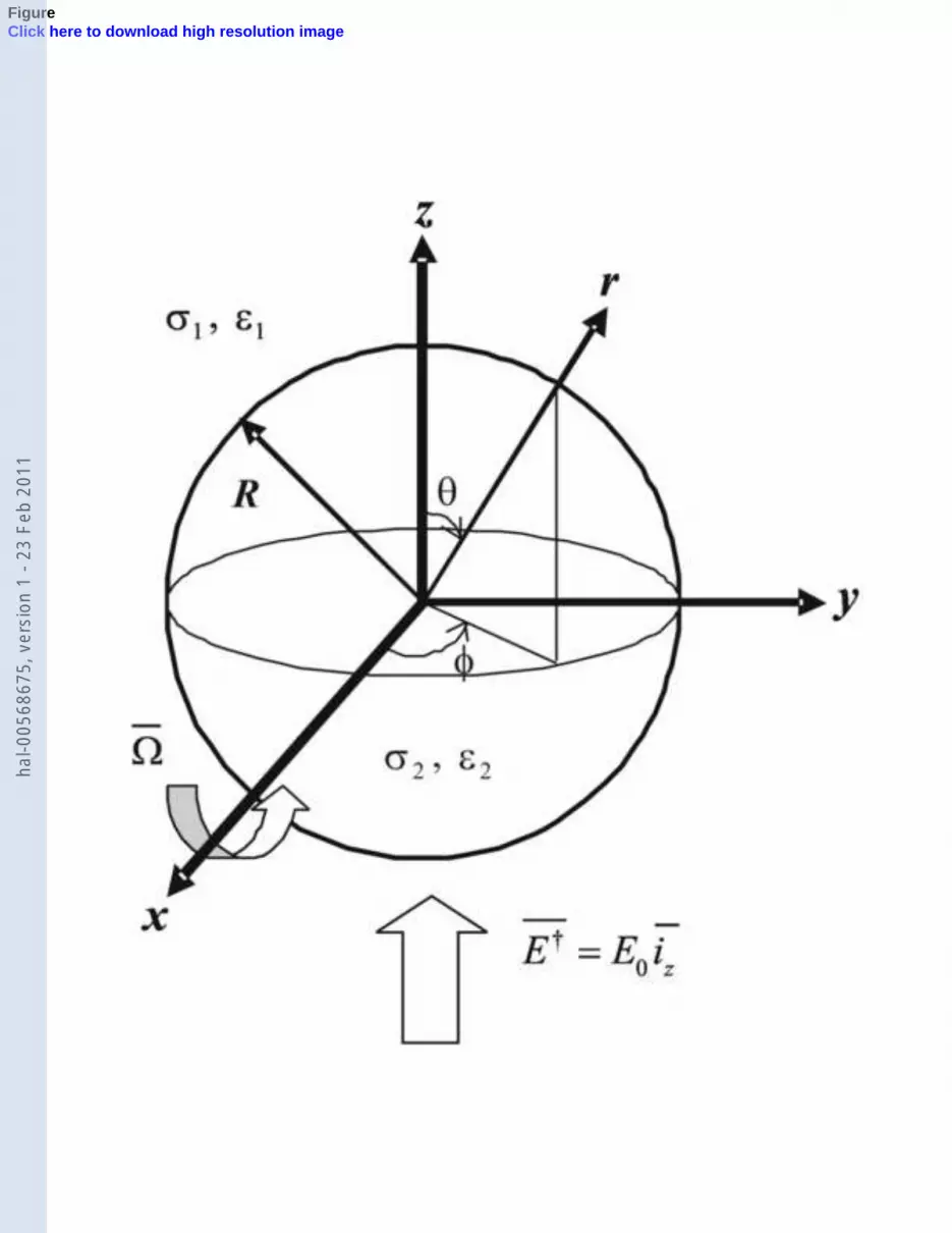
FigureClick here to download high resolution image

hal-0

0568

675,

ver

sion

1 -

23 F

eb 2

011

FigureClick here to download high resolution image

hal-0

0568

675,

ver

sion

1 -

23 F

eb 2

011

FigureClick here to download high resolution image

hal-0

0568

675,

ver

sion

1 -

23 F

eb 2

011

FigureClick here to download high resolution image

hal-0

0568

675,

ver

sion

1 -

23 F

eb 2

011

FigureClick here to download high resolution image

hal-0

0568

675,

ver

sion

1 -

23 F

eb 2

011

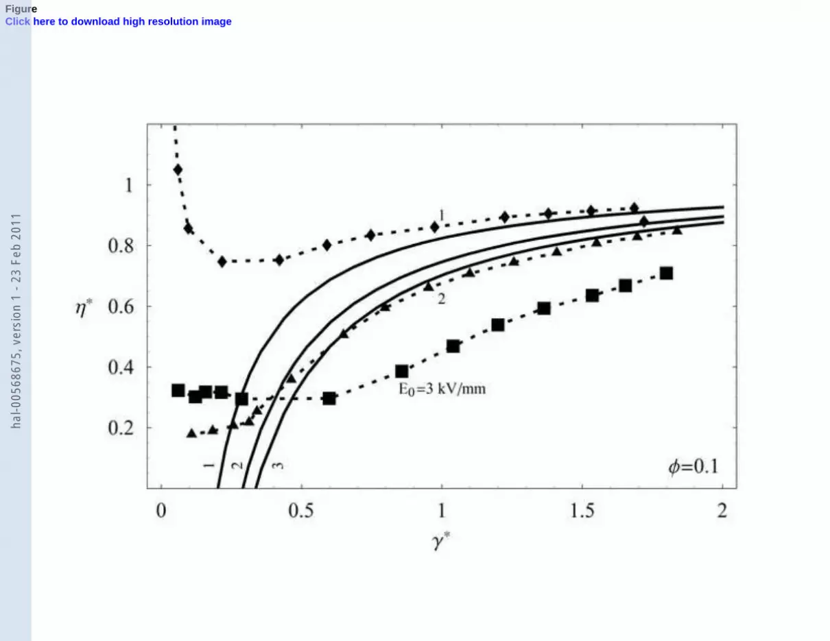
FigureClick here to download high resolution image

hal-0

0568

675,

ver

sion

1 -

23 F

eb 2

011

FigureClick here to download high resolution image

hal-0

0568

675,

ver

sion

1 -

23 F

eb 2

011

FigureClick here to download high resolution image

hal-0

0568

675,

ver

sion

1 -

23 F

eb 2

011

FigureClick here to download high resolution image

hal-0

0568

675,

ver

sion

1 -

23 F

eb 2

011

FigureClick here to download high resolution image

hal-0

0568

675,

ver

sion

1 -

23 F

eb 2

011

FigureClick here to download high resolution image

hal-0

0568

675,

ver

sion

1 -

23 F

eb 2

011

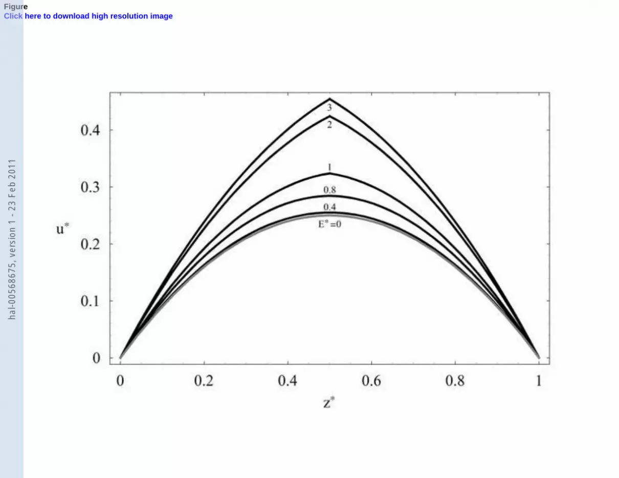
FigureClick here to download high resolution image

hal-0

0568

675,

ver

sion

1 -

23 F

eb 2

011

FigureClick here to download high resolution image

hal-0

0568

675,

ver

sion

1 -

23 F

eb 2

011

FigureClick here to download high resolution image

hal-0

0568

675,

ver

sion

1 -

23 F

eb 2

011

FigureClick here to download high resolution image

hal-0

0568

675,

ver

sion

1 -

23 F

eb 2

011