Journal of Non-Newtonian Fluid Mechanics 166 (2011) 839–846

Contents lists available at ScienceDirect

Journal of Non-Newtonian Fluid Mechanics

journal homepage: ht tp : / /www.elsevier .com/locate / jnnfm

The effect of wall slip on the stability of the Rayleigh–Bénard Poiseuille flowof viscoplastic fluids

Christel Métivier ⇑, Albert MagninLaboratoire de Rhéologie, UMR 5520 (Université Joseph Fourier, CNRS, Grenoble INP), Domaine Universitaire, BP 53, 38041 Grenoble Cedex, France

a r t i c l e i n f o

Article history:Received 8 February 2011Received in revised form 19 April 2011Accepted 21 April 2011Available online 29 April 2011

Keywords:Yield stress fluidWall slipStability analysisThermo-convection

0377-0257/$ - see front matter � 2011 Elsevier B.V. Adoi:10.1016/j.jnnfm.2011.04.017

⇑ Corresponding author. Tel.: +33 4 76825179.E-mail address: Christel.Metivier@ujf-grenoble.fr (

a b s t r a c t

This work investigates the effect of wall slip on the stability of the Bingham Rayleigh–Bénard Poiseuilleflow. The steady state of the Bingham plane Poiseuille flow is characterized by an unyielded region of 2yb

width and two sheared regions close to the walls with both no-slip and slip conditions at the walls. A lin-ear stability analysis of this flow with slip conditions is proposed in this paper. The slip boundary condi-tions case leads to flow destabilization compared with the results obtained in the no-slip case. Criticalconditions are modified by varying Cf , the friction number. For Cf < Oð1Þ, critical Rayleigh values Rac tendto that obtained with a free–free case (Cf tends to zero). For 10 < Cf < 30, Rac values decrease and reach aminimum in this zone. The value of Cf , for which Rac is minimal, varies slowly with the Bingham numberB. For Cf > 30 the flow is stabilized, i.e. Rac values increase and finally tend to that of the no-slip casewhen Cf > 1000. Furthermore, for 1 < Cf < 104, asymmetric modes were obtained. They are due to theslip boundary conditions at the walls.

� 2011 Elsevier B.V. All rights reserved.

1. Introduction

Slip occurs in flows of concentrated dispersions due to the dis-placement of the disperse phase away from solid walls. Slip effectsare usually observed when the disperse phase presents multi-mi-cron sized particles or droplets (emulsion) or has a high molecularweight (polymers). When sheared with smooth surfaces, the con-centrated dispersions exhibit apparent motion. Reviews on this to-pic have been proposed by Oldroyd [1] and Barnes [2]. Due to itspractical interest, the slip of non-Newtonian fluids is widely stud-ied. Numerous papers exist concerning observations of the slip ef-fect in the case of concentrated dispersions. In particular, the slip ofpolymer microgels in rheometers has been studied for a long time(e.g. [3–5]). Furthermore, recent papers [6,7] propose observationsand measurements of slip in pastes of soft particles as well as elas-tohydrodynamical lubricating models of slip taking into accountthe physico-chemical nature of the particle–wall interactions. Itis shown that the attractive paste–wall interactions exhibit no wallslip and a bulk yield stress, while the repulsive interactions exhibitslip velocities and low slip yield stress.

Pearson and Petrie [8] first introduced a slip boundary conditiongiving a relationship between the slip velocity at the wall and thewall shear stress. Fortin et al. [9] used this model in the followingform:

ll rights reserved.

C. Métivier).

bst ¼ � bcfbU t � s0

bU tbU t

��� ��� iff bU t

��� ���–0; ð1Þ

bst

�� �� < s0 iff bU t

��� ��� ¼ 0; ð2Þ

where the index t means tangential component; i.e. bU t ¼ bU � ðbU�nÞn and bst ¼ br � n� ½ðbr � nÞ � n�n, n being the unit outward vector.The hat notation is used for all dimensional variables. bcf and s0 rep-resent, respectively, the friction coefficient and the slip yield stress.Experiments show that slip occurs when bst

�� �� > s0, otherwise no-slipconditions are observed. s0 is found to be smaller than the bulk yieldstress bsy. The classical linear slip condition is found when s0 ¼ 0.The analogy between Eq. (2) and the constitutive law of a Binghamfluid can be observed. Indeed, for bs P bsy the Bingham model reads:

bs ¼ bsy

_bc þ blp

!_bc: ð3Þ

The effect of wall slip on the flow of viscoplastic fluids was stud-ied, for instance, by [10] who considered the Poiseuille flow in asquare pipe. By means of an adaptive finite-element method, thedifferent flow regimes are identified when the slip yield dimen-sionless number S, the friction number Cf and the yield stress num-ber B vary.

To our knowledge, the influence of slip conditions on the stabil-ity of flows involving viscoplastic fluids has never been studied.Only a few studies, e.g. [11–15] have been performed for Newto-nian fluids. This is not surprising, since Newtonian liquids slip in

840 C. Métivier, A. Magnin / Journal of Non-Newtonian Fluid Mechanics 166 (2011) 839–846

very few situations (e.g. small scale flow configurations or hydro-phobic solid surfaces). Considering a Newtonian plane Poiseuilleflow with Navier slip conditions at the walls, papers [11–13] pres-ent linear stability analyses and show that wall slip stabilizes theflow. In this configuration, the transition to turbulence is delayeddue to slip. However, [14,15] deal with the effect of slip boundarieson 2D thermal convection. They show that the flow is destabilizedwhen the slip increases at the walls.

The aim of the present paper is to investigate the effect of slipnear solid surfaces on the instability conditions when a viscoplasticfluid is involved. In particular, we propose to study the Rayleigh–Bénard Poiseuille (RBP) flow of a Bingham fluid.

The instability of the Bingham RBP flow is considered in the no-slip case in [16,17]. In these studies, the effect of the yield stress oncritical conditions and on the evolution of the amplitude perturba-tion is investigated using linear and weakly non-linear stabilityanalyses, respectively. Here, we propose to extend the study of[16] by considering slip conditions at the walls. In this respect, alinear stability analysis is developed considering dominant buoy-ancy forces, i.e. small values of the Reynolds number Re.

In Section 2, all the governing equations are presented includingthe development of the steady state solution (Section 2.1) and theperturbation set of linearized equations (Section 2.2). The thirdsection presents the numerical results as well as a discussion.The effect of the dimensionless numbers S and Cf , is investigatedand the results are compared with the no-slip configuration. Thepaper ends with a concluding section.

2. Governing equations

We consider the Poiseuille flow under an imposed axial pres-sure gradient of a yield stress fluid in a horizontal plane channel.The upper and lower walls are at constant temperatures,bT 0 � dbT=2 and bT 0 þ dbT=2, respectively.

The dimensionless problem is obtained using the width bL of theplane channel as length-scale, and the thermal diffusion time bL2=babetween the two walls as the timescale; here ba is the thermal dif-fusivity of the fluid. In order to compare the slip conditions withthe no-slip case, the maximum velocity bU0 of the no-slip boundaryconditions is used as the velocity scale. The stress and pressurescale is thus bl0

bU0=bL, with bl0 being the plastic viscosity. Withthe Boussinesq approximation, the governing equations read:

$ � U ¼ 0; ð4aÞReUt þ Re2 Pr U � $ð ÞU ¼ RePr �$P þ $ � sð Þ þ RaT ey; ð4bÞTt þ RePr U � $ð ÞT ¼ r2T; ð4cÞ

where, U corresponds to the velocity vector, T is the reduced tem-perature scaled with dbT , P the modified pressure, and s the devia-toric stress tensor. The velocity vector U is of the formU ¼ U ex þ V ey þW ez, where U;V and W are the velocity compo-nents and ex; ey; ez are unit vectors in the streamwise, transverseand spanwise directions, respectively.

The dimensionless numbers are the Reynolds, Re ¼bq bU0

bLbl0, Pra-

ndtl, Pr ¼bl0bqba and Rayleigh, Ra ¼

bqca0 gdbTbL3bl0ba numbers, bq is the fluid

density, ca0 is the thermal expansion coefficient and g the gravita-tional acceleration.

As a remark, the scales chosen in this study are similar to thoseof the no-slip walls case. In this sense, the effect of the boundaryslip could be directly compared with the results shown in [17].

The constitutive law for a Bingham fluid is given by:

s ¼ l _c iff s > B; ð5Þ_c ¼ 0 iff s 6 B; ð6Þ

with l ¼ 1þ B_c the effective viscosity and B ¼ bs0

bL= bl0bU0

� �the

Bingham number. The rate of strain tensor is denoted by _c; _c ands are the second invariants of the rate of strain and deviatoric stresstensors, respectively.

The set of Eq. (4) is completed by the boundary conditions at thewalls with constant temperatures:

Tð�1=2Þ ¼ T1 ¼ 1=2 and Tð1=2Þ ¼ T2 ¼ �1=2; ð7Þ

the wall slip is described as follows:

Utð�1=2Þ ¼ � stð�1=2ÞCf

1� Sstð�1=2Þj j

� �iff stð�1=2Þj j > S; ð8Þ

Utð�1=2Þ ¼ 0 iff stð�1=2Þj j 6 S; ð9Þ

where the notation �j j represents the vector norm vj j ¼ ðv � vÞ1=2. Inthe two-dimensional case, these conditions read:

Uð�1=2Þ¼�sxyð�1=2ÞCf

1� Ssxyð�1=2Þ�� ��

" #iff sxyð�1=2Þ

�� ��> S; ð10Þ

Uð�1=2Þ¼0 iff sxyð�1=2Þ�� ��6 S: ð11Þ

The slip yield number S and the friction number Cf are defined,respectively, by:

S ¼ s0bLbl0bU0

and Cf ¼bcfbLbl0;

Finally, the boundary condition expressing the fact that the fluiddoes not cross the walls is given by:

U � n ¼ 0: ð12Þ

2.1. Fully developed flow

The steady state flow leads to a basic conductive state with alinear temperature profile given as follows

Tb ¼ �y: ð13Þ

The pressure is given by:

Pbðx; yÞ ¼ Pref �y2

2Ra

RePr� 2

1=2� ybð Þ2x; ð14Þ

where Pref corresponds to a reference pressure. The stress field isdescribed by the only non-zero component sxy:

sbxy ¼@p@x

y ¼ � 2

ð1=2� ybÞ2 y ð15Þ

and the velocity Ub ¼ ðUbðyÞ;0; 0Þ reads:

UbðyÞ ¼1þ 1

Cf

B2ybþ S

� �for jyj 6 yb

1� jyj � yb

1=2� yb

� �2

þ 1Cf

B2ybþ S

� �for yb < yj j < 1=2;

8>>><>>>:ð16Þ

where 2yb is the width of the central unyielded region as shown in

Fig. 1. In Eq. (16), it can be seen that Us ¼1Cf

B2ybþ S

� �corresponds

to the wall slip velocity. Us varies non-linearly with Cf and S asshown in Eq. (16) as well as in Fig. 1 which shows velocity profilesfor different values of Cf and S. The decrease in the friction coeffi-cient as well as the increase in the value of S lead to an increasein the slip velocity value Us. The no-slip case is recovered forUs ¼ 0, i.e. Cf !1 and S ¼ 0. The limit case Cf ! 0, for which thefriction effect is very weak, will be denoted as the free-free casein the following. The distinction is made with the perfect slip case.

Fig. 1. Velocity profiles for yb ¼ 0:1 ðB ¼ 1:25Þ and different values of Cf and S. Thegray zone represents the unyielded region. Dotted lines: S ¼ 5; Cf ¼ 50, dashedlines: S ¼ 5; Cf ¼ 2, dash-dotted lines: S ¼ 0:5; Cf ¼ 50, solid lines: S ¼ 0:5; Cf ¼ 2.

C. Métivier, A. Magnin / Journal of Non-Newtonian Fluid Mechanics 166 (2011) 839–846 841

Indeed, the perfect slip case leads to an entire unyielded flow whichis linearly stable.

In addition, the yield surfaces position depends on the Binghamnumber B via the following relation:

B ¼ 2yb

ðyb � 1=2Þ2: ð17Þ

Finally, comparing the two cases, i.e. no-slip boundary condi-tions and slip boundary conditions, the only difference is the valueof the mean velocity which is increased by Us when slip occurs atwalls. One can notice that, with B constant, the shear rate andstress fields are not modified in either case. In particular, the wallstress value is sw ¼ B=ð2ybÞ > B. As a consequence, the viscosityprofile is also similar in the yielded regions.

2.2. Linear stability analysis

A small perturbation Aðw;H; p;�y�i Þ is introduced into the fullydeveloped flow. Here, A corresponds to the amplitude of the per-turbation and w is the stream function, defined by u ¼ @yw andv ¼ �@xw. The perturbation field is sought in the following form:

w; �y�i ; p; H

¼ f ðyÞ; �y�1 ; pðyÞ; hðyÞ

ei a ðx�ctÞ; ð18Þ

where a denotes the streamwise wave number and aci ¼ ImðxÞ de-notes the growth rate.

Considering Eq. (18), the linearized equations of the perturba-tions (vorticity and energy equations) represent a generalizedeigenvalue problem, with c being the eigenvalue.

In the two yielded regions, the eigenvalue problem is writtenas:

L1f þ L2h ¼ cL3f ; ð19aÞL4 hþ f ¼ ch; ð19bÞ

with L1; L2; L3 and L4, the following operators:

L1�PrRe UbðD2�a2Þ�D2Ub

h iþPri

aðD2�a2Þ2�4iaPrBD

DjDUbj

� �;

L2�PrRa;

L3�D2�a2;

L4�PrReUb� iaþ ia

D2;

ð20Þ

where D � @y.

In the unyielded region, by combining the translation of theplug zone, in particular one writes @xUðx; y�i ; tÞ ¼ 0, and the normalmode assumption leads to f ¼ u ¼ v ¼ 0. In this zone, the eigen-value problem is reduced to:

f ¼ 0; ð21aÞL4 h ¼ ch: ð21bÞ

At the yield surfaces ðy ¼ y�i Þ, the yield conditions lead to:

f ð�ybÞ ¼ Df ð�ybÞ ¼ 0 ð22Þ

and

D2f ð�ybÞ ¼ �y�1 D2Ubð�ybÞ: ð23Þ

Actually, this last equation gives a condition for y1, not for f.At the walls ðy ¼ �1=2Þ, the constant temperature conditions

read:

hð�1=2Þ ¼ 0: ð24Þ

At first order, the slip conditions, uð�1=2Þ ¼ �s0xyð�1=2Þ

Cf, can also

be written as follows:

D2f þ Cf Df � a2fh i

�1=2¼ 0: ð25Þ

In addition, the fact that the fluid does not cross the walls reads:

vð�1=2Þ ¼ �f ð�1=2Þ ¼ 0: ð26Þ

Remarks:

(i) The no-slip case involves the same perturbation equationsand boundary conditions except condition Eq. (25). Indeed,in the no-slip case, one obtains f ð�1=2Þ ¼ Df ð�1=2Þ ¼ 0.

(ii) In the slip case, the asymptotic conditions lead to the follow-ing boundary conditions at the walls:

� For Cf ! 0

f ð�1=2Þ ¼ D2f ð�1=2Þ ¼ 0: ð27Þ

These conditions correspond to the free–free case.

� For Cf !1

f ð�1=2Þ ¼ Df ð�1=2Þ ¼ 0 ð28Þ

These conditions are similar to no-slip boundary conditions.

3. Results and discussion

The set of Eqs. (19)–(26) is solved numerically by means of a fi-nite difference method. A second-order centered finite scheme isused in order to discretize the equations. The resulting problemrepresents an eigenvalue problem which is solved using the QZalgorithm implemented in Matlab 7.1. The numerical code wastested for the no-slip case, by comparing with the Newtonian case.The results converge for N ¼ 201 nodes, for which the Newtonianresults [18] are recovered with a discrepancy of 0.5%. Consideringthe Bingham Rayleigh–Bénard Poiseuille flow with slip boundaryconditions, the results converge for N ¼ 301.

A resulting spectrum of the slip configuration is presented inFig. 2a for S ¼ 2 and Cf ¼ 2. The spectrum is plotted at criticalityand is comparable to the one obtained in the no-slip configurationas shown in Fig. 2b. The increase in the velocity phase can be ob-served, through the increase in cr , in the slip case compared withthe no slip case. This is due to the increase in the mean velocityof the basic flow.

Fig. 2. Spectrum of the largest eigenvalues for Re ¼ 0:01, Pr ¼ 50, yb ¼ 0:1ðB ¼ 1:25Þ.

Fig. 3. Critical Rayleigh number as a function of the Bingham number for differentvalues of S and Cf ¼ 2, Re ¼ 0:01 (j: No-slip case, r: S ¼ 0, �: S ¼ 0:5, D: S ¼ 2, �:S ¼ 5, �: S ¼ 8).

Fig. 4. Critical Rayleigh number as a function of the Bingham number for differentvalues of the friction number Cf and S ¼ 2, Re ¼ 0:01 (j: No-slip case, �:Cf ¼ 0:001, D: Cf ¼ 0:01, �: Cf ¼ 5, �: Cf ¼ 15, �: Cf ¼ 20, r: Cf ¼ 50, : Cf ¼ 100).

842 C. Métivier, A. Magnin / Journal of Non-Newtonian Fluid Mechanics 166 (2011) 839–846

Critical Rayleigh numbers are presented in Fig. 3 as a function ofthe Bingham number for Cf ¼ 2 and different values of S. In this fig-ure, the no-slip case is represented by black squares and somesymbols (circles and diamonds) corresponding to S ¼ 5 and S ¼ 8,since for low values of B the Von Mises criterion leads to a no-slipcondition, i.e. sw 6 S (Eq. (11)). The figure shows that slip condi-tions at the walls destabilize the flow decreasing the values ofRac . With respect to S ¼ 5 and S ¼ 8, the variations in Rac are dueonly to stick-slip: either the fluid sticks at the walls ðsw 6 SÞ withlow B or it slips ðsw > SÞ, since sw depends on B. In the both slipand no-slip cases, the Newtonian critical conditions are not recov-ered for B! 0. This is due to the presence of the central plug zonein which the velocity perturbation vanishes (see [19] for furtherdetails). On the other hand, if only slip conditions are considered,one notices that variations in S do not modify the values of the crit-ical conditions since Rac remains constant by varying S, even in thelimit case S ¼ 0. This is not surprising since the stress is weaklyperturbed. In this sense the perturbed stress value remains closeto that of the basic state, in particular at the wallssxyð�1=2Þ ¼ sw > S. Furthermore, S does not have any influenceon the stability analysis, i.e. Eqs. (19)–(26).

The influence of the variations in Cf is also investigated. Fig. 4represents critical conditions for different values of the frictionnumber Cf with S ¼ 2. The only cases considered with this value

of S are those in which the fluid slips at the walls, for all B. As saidbefore, slip conditions at the walls destabilize the flow since theRac values are smaller than that of the no-slip case (black squares).For Cf > 30, critical conditions tend to that obtained in the no-slipcase while for Cf < 10, the Rac values tend to the free-free case. Atransition region is observed for 10 < Cf < 30. Actually, in thisrange of values, one observes that (i) if B < Bc , Bc a critical value,then the Rac values tend to the no-slip conditions, (ii) if B > Bc , alarge variation is observed in Rac and the flow is destabilized asshown in Fig. 4 (see circles and diamonds with dashed lines). Fur-thermore, it can be seen that Bc varies slightly with Cf as is alsounderlined in Fig. 5 (dashed lines). This figure, which representsRac as a function of Cf for different values of B, confirms that thevariation in critical values, comparing the slip and the no-slipcases, is more significant in this transition region. With fixed val-ues of B, one notices that Rac is constant when Cf < Oð1Þ and isequal to the value obtained for the limit case Cf ! 0, i.e. thefree–free case. For 10 < Cf < 30, the values of Rac decrease, reacha minimum at Cfm ¼ Oð10Þ and then increase significantly. Finally,the Rac values tend to that of the no-slip case with high values of Cf

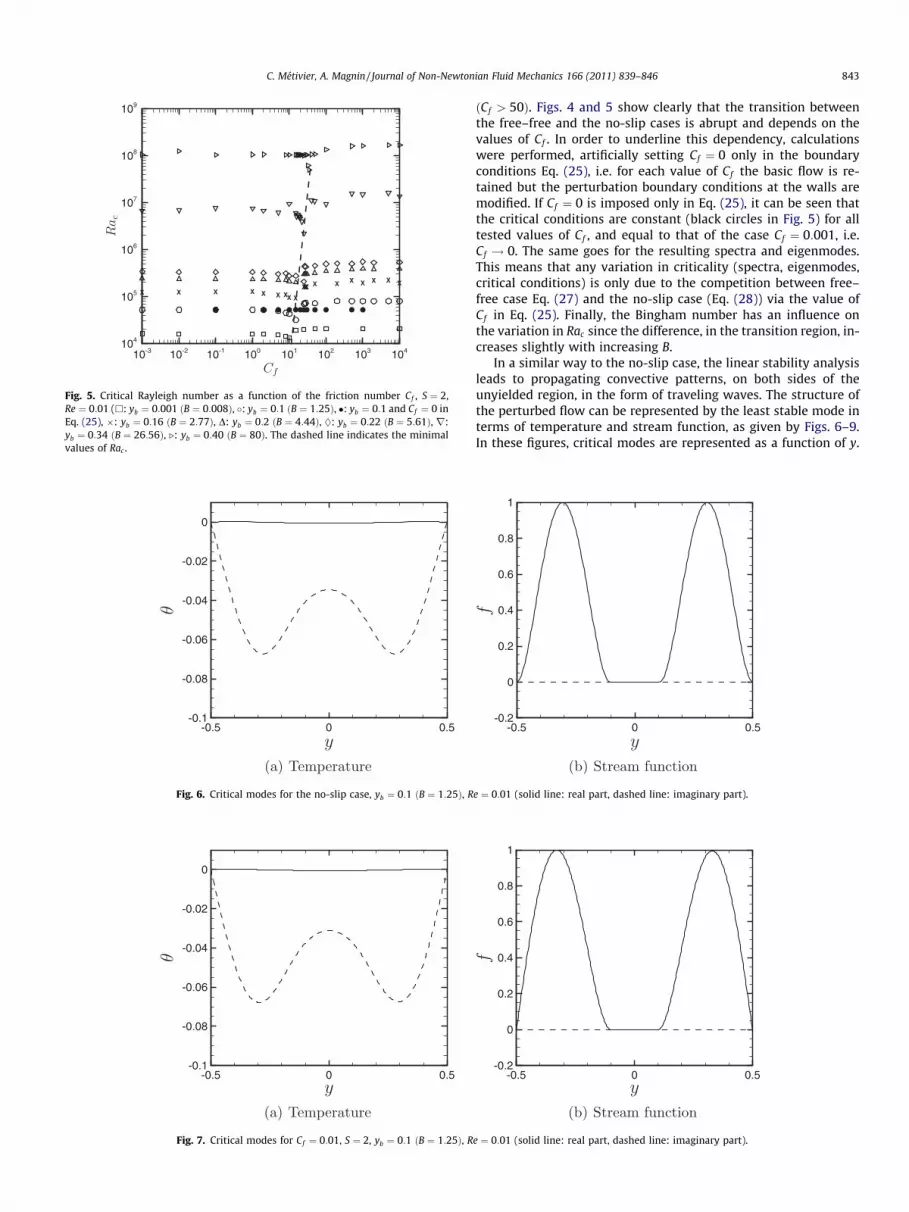
Fig. 5. Critical Rayleigh number as a function of the friction number Cf , S ¼ 2,Re ¼ 0:01 (h: yb ¼ 0:001 ðB ¼ 0:008Þ, �: yb ¼ 0:1 ðB ¼ 1:25Þ, �: yb ¼ 0:1 and Cf ¼ 0 inEq. (25), : yb ¼ 0:16 ðB ¼ 2:77Þ, D: yb ¼ 0:2 ðB ¼ 4:44Þ, �: yb ¼ 0:22 ðB ¼ 5:61Þ, r:yb ¼ 0:34 ðB ¼ 26:56Þ, .: yb ¼ 0:40 ðB ¼ 80Þ. The dashed line indicates the minimalvalues of Rac .

Fig. 6. Critical modes for the no-slip case, yb ¼ 0:1 ðB ¼ 1:25Þ, R

Fig. 7. Critical modes for Cf ¼ 0:01, S ¼ 2, yb ¼ 0:1 ðB ¼ 1:25Þ, R

C. Métivier, A. Magnin / Journal of Non-Newtonian Fluid Mechanics 166 (2011) 839–846 843

ðCf > 50Þ. Figs. 4 and 5 show clearly that the transition betweenthe free–free and the no-slip cases is abrupt and depends on thevalues of Cf . In order to underline this dependency, calculationswere performed, artificially setting Cf ¼ 0 only in the boundaryconditions Eq. (25), i.e. for each value of Cf the basic flow is re-tained but the perturbation boundary conditions at the walls aremodified. If Cf ¼ 0 is imposed only in Eq. (25), it can be seen thatthe critical conditions are constant (black circles in Fig. 5) for alltested values of Cf , and equal to that of the case Cf ¼ 0:001, i.e.Cf ! 0. The same goes for the resulting spectra and eigenmodes.This means that any variation in criticality (spectra, eigenmodes,critical conditions) is only due to the competition between free–free case Eq. (27) and the no-slip case (Eq. (28)) via the value ofCf in Eq. (25). Finally, the Bingham number has an influence onthe variation in Rac since the difference, in the transition region, in-creases slightly with increasing B.

In a similar way to the no-slip case, the linear stability analysisleads to propagating convective patterns, on both sides of theunyielded region, in the form of traveling waves. The structure ofthe perturbed flow can be represented by the least stable mode interms of temperature and stream function, as given by Figs. 6–9.In these figures, critical modes are represented as a function of y.

e ¼ 0:01 (solid line: real part, dashed line: imaginary part).

e ¼ 0:01 (solid line: real part, dashed line: imaginary part).

Fig. 8. Critical modes for different values of Cf , S ¼ 2, yb ¼ 0:1 ðB ¼ 1:25Þ, Re ¼ 0:01 (solid line: Cf ¼ 10, long dashed line: Cf ¼ 5, dash-dotted line: Cf ¼ 2, dashed line: Cf ¼ 1).

Fig. 9. Critical modes for S ¼ 2, yb ¼ 0:1 ðB ¼ 1:25Þ, Re ¼ 0:01 (solid line: Cf ¼ 100, dash-dotted line: Cf ¼ 50, dashed line: Cf ¼ 30, long-dashed line: Cf ¼ 25).

Fig. 10. Critical modes for S ¼ 2, yb ¼ 0:1 ðB ¼ 1:25Þ, Re ¼ 0:01 (solid line: Cf ¼ 200, dashed line: Cf ¼ 500, dash-dotted line: Cf ¼ 1000, long-dashed line: Cf ¼ 10000).

844 C. Métivier, A. Magnin / Journal of Non-Newtonian Fluid Mechanics 166 (2011) 839–846

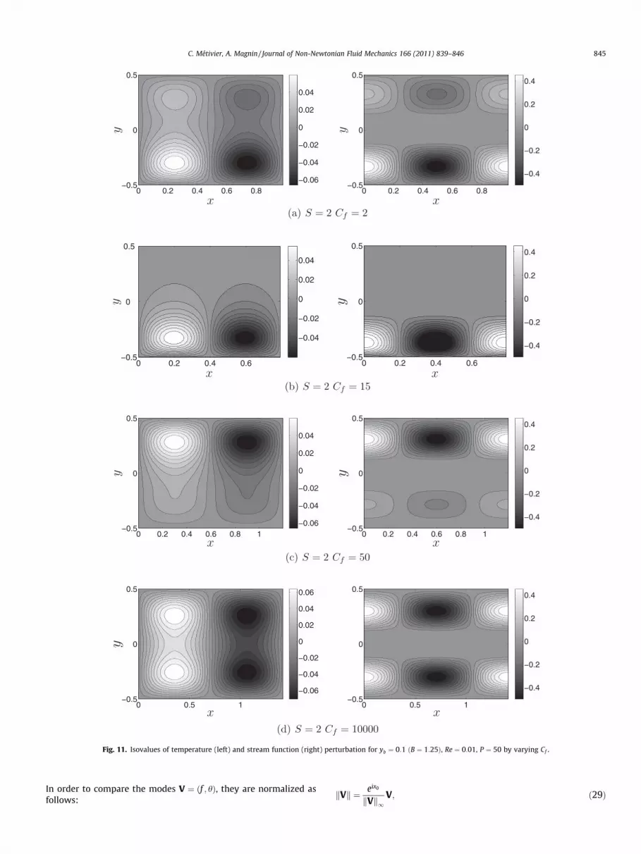
Fig. 11. Isovalues of temperature (left) and stream function (right) perturbation for yb ¼ 0:1 ðB ¼ 1:25Þ, Re ¼ 0:01, P ¼ 50 by varying Cf .

C. Métivier, A. Magnin / Journal of Non-Newtonian Fluid Mechanics 166 (2011) 839–846 845

In order to compare the modes V ¼ ðf ; hÞ, they are normalized asfollows:

kVk ¼ eix0

kVk1V; ð29Þ

846 C. Métivier, A. Magnin / Journal of Non-Newtonian Fluid Mechanics 166 (2011) 839–846

with kVk1 ¼maxy

ffiffiffiffiffiffiffiffiffiffiffiffiffiffiffiffiffiffiffiffiffiffiffiffiffiffiffiffiffiffiffiffiffiffiffiffiReðVÞ2 þ ImðVÞ2

q, the norm infinity, and

x0 ¼ Arctan � ImðkVk1ÞReðkVk1Þ

� �, the reference phase.

Fig. 6 shows the critical modes obtained in the no-slip case. Themodes are found to be symmetric and the maximum amplitude ofthe perturbation is attained by the real part of the stream functionin the middle of each yielded region.

For low values of Cf , i.e. Cf < 0:1, the critical modes are alsosymmetric, as shown in Fig. 7. However, a difference with theno-slip configuration can be observed via the derivative of f atthe walls given by the boundary conditions Eq. (27) whenCf ! 0. This is in agreement with the decrease in Rac in the Ray-leigh–Bénard Newtonian case (see [20]) when the (no-slip) rigidsurfaces case ðRac ¼ 1707:76Þ is compared with the perfect slipcase ðRac ¼ 657:51Þ.

Asymmetric modes can be observed for 1 < Cf < 104, as repre-sented in Figs. 8–10. The increase in the values of Cf increasesthe differences between the extrema of the mode f in the twoyielded regions. On the other hand, this increasing asymmetric ef-fect goes with a mean decrease in the intensity of the perturbationvia f and h. As said before, the asymmetry does not involve signif-icant variations in Rac , if the results obtained by varying Cf from 1to 10 are compared.

Furthermore, with increasing Cf values, the break in symmetryis still observed even when 10 < Cf < 104 while the Rac values tendto those obtained in the no-slip configuration as shown in Fig. 9.Actually, the modes obtained in the no-slip configuration can berecovered with larger values of Cf , that is to say Cf ¼ Oð104Þ, ascan be seen in Fig. 10. As expected, for Cf !1, the no-slip caseis recovered in terms of critical conditions as well as flow condi-tions, e.g. the perturbation modes.

Furthermore, the thermoconvective rolls are depicted via theisovalues of normal modes W and H in Fig. 11. Obviously, theasymmetry of the modes is also observed via a decrease in theintensity of the perturbation in one yielded region: either theupper one or the lower one depending on whether Cf values arelow or large, respectively.

The origin of the asymmetry in terms of perturbation modes isdue only to Cf . Actually, as said before, when Cf is artificially set tozero in boundary condition Eq. (25), the perturbation modes aresymmetric and are similar to the ones obtained with Cf ¼ 0:01(Fig. 7). The asymmetry of the modes is due only to the competi-tion between the (derivatives at the walls of the) modes obtainedin the no-slip case (Fig. 6) and the ones obtained in the free–freecase (Fig. 7) via the value of Cf in Eq. (25).

4. Conclusion

The linear stability of the plane Bingham Rayleigh–BénardPoiseuille flow was studied considering slip conditions at the walls.The effect of the two dimensionless numbers S and Cf , which char-acterize the wall slip, was investigated. The numerical results showthat the wall slip leads to destabilize the flow since the critical Ray-leigh values are smaller than the ones obtained in the no-slip case.In the range of values tested, one observes that variations in S donot modify the critical conditions, while variations in Cf do. We

showed that (i) for Cf < Oð1Þ, the critical conditions tend to thefree–free case, (ii) for Cf > 30, the critical Rayleigh values increase,(iii) the no-slip case is recovered in terms of critical conditionswhen Cf P 100. The effect of Cf was also underlined via the pertur-bation modes. In a range of values such as 10 < Cf < 104, asym-metric modes were observed in terms of stream function andtemperature. This is clearly the consequence of the competitionbetween the free–free case and the no-slip case through the slipconditions Eq. (25).

In conclusion, it is of great importance to pay attention to wallconditions, in particular in experiments, since critical conditionscan be modified by considering either no-slip or slip conditions.

Acknowledgments

The authors’ work was supported by the French National Re-search Agency (ANR), via the grant called ‘‘ThiM’’. The authorsare also grateful to the Research Group AmeTH.

References

[1] J.G. Oldroyd, Non-Newtonian flow of solids and liquids, in: F.R. Eirich (Ed.),Rheology: Theory and Applications, vol. 1, Academic Press Inc., New York,1956, pp. 653–682.

[2] H.A. Barnes, A review of the slip (wall depletion) of polymers solutions,emulsions and particle suspensions in viscosimeters: it causes, character, andcure, J. Non-Newtonian Fluid Mech. 36 (1995) 85–108.

[3] G.V. Vinogradov, G.B. Froisheter, K.K. Trilisky, The flow of plastic dispersesystems in the presence of the wall effect, Rheol. Acta 14 (9) (1975) 765.

[4] A. Magnin, J.M. Piau, Cone-and-plate rheometry of yield stress fluids. Study ofan aqueous gel, J. Non-Newtonian Fluid Mech. 56 (1990) 221–251.

[5] J.M. Piau, Carbopol gels: elastoviscoplastic and slippery glasses made ofindividual swollen sponges. Meso- and macroscopic properties, constitutiveequations and scaling laws, J. Non-Newtonian Fluid Mech. 144 (2007) 1–29.

[6] S.P. Meeker, R.T. Bonnecaze, M. Cloitre, Slip and flow in soft particles pastes,Phys. Rev. Lett. 92 (19) (2004) 198302.

[7] J.R. Seth, M. Cloitre, R.T. Bonnecaze, Influence of short-range forces on wall-slipin microgel pastes, J. Rheol. 52 (5) (2008) 1241–1268.

[8] J.R.A. Pearson, C.J.S. Petrie, in: Proceedings of the Fourth International Congresson Rheology, Part 3, Wiley, New York, 1965.

[9] A. Fortin, D. Cté, P.A. Tanguy, On the imposition of friction boundary conditionsfor the numerical simulation of Bingham fluid flows, Comput. Meth. Appl.Mech. Eng. 88 (1991) 97109.

[10] N. Roquet, P. Saramito, An adaptative finite element method for viscoplasticflows in a square pipe with stick-slip at the wall, J. Non-Newtonian Fluid Mech.155 (2008) 101–115.

[11] J.M. Gersting, Hydrodynamic stability of plane porous slip flow, Phys. Fluids 17(2126) (1974).

[12] E. Lauga, C. Cossu, A note on the stability of slip channel flows, Phys. Fluids 17(088106) (2005).

[13] T. Min, J. Kim, Effects of hydrophobic surface on stability and transition, Phys.Fluids 17 (108106) (2005).

[14] L.S. Kuo, P.H. Chen, Effects of slip boundary conditions on Rayleigh–Bénardconvection, J. Mech. 25 (2009) 205–212.

[15] L.S. Kuo, W.P. Chou, P.H. Chen, Effects of slip boundaries on thermal convectionin 2D box using Lattice Boltzmann method, Int. J. Heat Mass Transfer 52 (2011)1340–1343.

[16] C. Métivier, C. Nouar, On linear stability of Rayleigh–Bénard Poiseuille flow ofviscoplastic fluids, Phys. Fluids 20 (104101) (2008).

[17] C. Métivier, C. Nouar, J.P. Brancher, Weakly nonlinear dynamics ofthermoconvective instability involving viscoplastic fluids, J. Fluid Mech. 660(2010) 316–353.

[18] X. Nicolas, Revue bibliographique sur les écoulements de Poiseuille-Rayleigh-Bénard: écoulements de convection mixte en conduites rectangulaireshorizontales chauffées par le bas, Int. J. Heat Mass Transfer 43 (2000) 589.

[19] C. Métivier, C. Nouar, J.P. Brancher, Linear stability involving the Binghammodel when the yield stress approaches zero, Phys. Fluids 17 (104106) (2005).

[20] S. Chandrasekhar, Hydrodynamic and Hydromagnetic Stability, ClarendonPress, Oxford, 1961.