Convergence analysis of the Bregman method for the variational model of image denoising

Appl. Comput. Harmon. Anal. 27 (2009) 367–379

Contents lists available at ScienceDirect

Applied and Computational Harmonic Analysis

www.elsevier.com/locate/acha

Letter to the Editor

Convergence analysis of the Bregman method for the variational model ofimage denoising ✩

Rong-Qing Jia ∗, Hanqing Zhao, Wei Zhao

Department of Mathematical and Statistical Sciences, University of Alberta, Edmonton, Canada T6G 2G1

a r t i c l e i n f o a b s t r a c t

Article history:Available online 13 May 2009Communicated by Charles K. Chuion 3 October 2008

Keywords:Bregman methodOptimizationTotal variationImage denoisingWavelet packets

The total variation model of Rudin, Osher, and Fatemi for image denoising is considered tobe one of the best denoising models. Recently, by using the Bregman method, Goldsteinand Osher obtained a very efficient algorithm for the solution of the ROF model. In thispaper, we give a rigorous proof for the convergence of the Bregman method. We alsoindicate that a combination of the Bregman method with wavelet packet decompositionoften enhances performance for certain texture rich images.

© 2009 Elsevier Inc. All rights reserved.

1. Introduction

The TV (total variation) model of Rudin, Osher, and Fatemi [14] for image denoising is considered to be one of the bestdenoising models. Recently, using the Bregman method, Goldstein and Osher [9] provided a very efficient algorithm for thesolution of the ROF model. In this paper, we give a rigorous proof for the convergence of the Bregman method. Moreover, forcertain texture rich images, we also discuss some improvements of the ROF model by using a combination of the Bregmanmethod with wavelet packet decomposition.

An image is regarded as a function

u : {1, . . . , N} × {1, . . . , N} → R,

where N � 2. Suppose u ∈ RN2 = R

{1,...,N}×{1,...,N} . For 1 � p < ∞, let

‖u‖p :=( ∑

1�i, j�N

∣∣u(i, j)∣∣p

)1/p

,

and let ‖u‖∞ := max1�i, j�N |u(i, j)|. We use ∇x to denote the difference operator given by ∇xu(1, j) = 0 for j = 1, . . . , Nand

∇xu(i, j) = u(i, j) − u(i − 1, j), i = 2, . . . , N, j = 1, . . . , N.

✩ Supported in part by NSERC Canada under Grant OGP 121336.

* Corresponding author.E-mail addresses: [email protected] (R.-Q. Jia), [email protected] (H. Zhao), [email protected] (W. Zhao).

1063-5203/$ – see front matter © 2009 Elsevier Inc. All rights reserved.doi:10.1016/j.acha.2009.05.002

http://www.ScienceDirect.com/

http://www.elsevier.com/locate/acha

mailto:[email protected]



http://dx.doi.org/10.1016/j.acha.2009.05.002

368 R.-Q. Jia et al. / Appl. Comput. Harmon. Anal. 27 (2009) 367–379

Then ∇x is a linear mapping from RN2

to RN2

. Similarly, ∇y is the difference operator from RN2

to RN2

given by∇yu(i,1) = 0 for i = 1, . . . , N and

∇yu(i, j) = u(i, j) − u(i, j − 1), i = 1, . . . , N, j = 2, . . . , N.

The total variation of u is represented by

‖∇xu‖1 + ‖∇yu‖1 or∥∥√

(∇xu)2 + (∇yu)2∥∥

1.

Let f ∈ RN2

be an observed image with noise. We wish to recover a target image u from f by denoising. The anisotropicTV model for denoising can be formulated as the following minimization problem:

minu

[‖∇xu‖1 + ‖∇yu‖1 + μ

2‖u − f ‖2

2

], (1.1)

where μ is an appropriately chosen positive parameter. Correspondingly, the isotropic TV model for denoising is the follow-ing minimization problem:

minu

{∥∥√(∇xu)2 + (∇yu)2

∥∥1 + μ

2‖u − f ‖2

2

}. (1.2)

This motivates us to consider the general minimization problem of a convex function on the n-dimensional Euclideanspace R

n . Let E : Rn → R be a continuous and convex function. A vector g in R

n is called a subgradient of E at a pointv ∈ R

n if

E(u) − E(v) − 〈g, u − v〉 � 0 ∀u ∈ Rn.

The subdifferential ∂ E(v) is the set of subgradients of E at v . It is known that the subdifferential of a convex function at anypoint is nonempty. Clearly, v is a minimal point of E if and only if 0 ∈ ∂ E(v). If this is the case, we write

v = arg minu

{E(u)

}.

The Bregman distance associated with E at v is

D gE (u, v) := E(u) − E(v) − 〈g, u − v〉,

where g is a subgradient of E at v . Clearly, D gE (u, v) � 0. Moreover, D g

E (u, v) � D gE (w, v) for any w on the line segment

between u and v .Let E and H be two convex functions from R

n to R. Suppose that E is continuous and H is continuously differentiable.By abuse of notation, ∂ H(v) is also used to denote the gradient of H at a point v ∈ R

n . We start with initial vectors g0 andu0 in R

n . For k = 0,1,2, . . . , let

uk+1 := arg minu

[E(u) − ⟨

gk, u − uk⟩ + H(u)]

(1.3)

and

gk+1 := gk − ∂ H(uk+1). (1.4)

This is called the Bregman iteration, as was suggested in [1]. In the preceding process we have assumed the existence ofsolutions to the minimization problem in (1.3).

Let A = (aij)1�i�m,1� j�n be an m × n matrix with its entries in R. We assume that the rank of A is m. The matrix Ainduces the linear mapping from R

n to Rm given by A[u1, . . . , un]T = [v1, . . . , vm]T with

vi =n∑

j=1

aiju j, i = 1, . . . ,m.

Here and in what follows, we use the superscript T to denote the transpose of a matrix. Given a vector b in the range of A,we wish to find

minu

E(u) subject to Au = b. (1.5)

For the case when E(u) = ‖u‖1, Bregman iterative algorithms for the above minimization problem was analyzed in [20]by Yin et al. Among other things, they showed that the iterative approach yields exact solutions in a finite number of steps.Note that in this case solutions are not unique. For the minimization problems considered in this paper, in general, thesolutions will not be achieved in a finite number of Bregman iterations.

Suppose that the minimization problem (1.5) has a unique solution u. For λ > 0, set H(u) := (λ/2)‖Au − b‖22. Let

(uk+1)k=0,1,... be the sequence given by the Bregman iteration (1.3) and (1.4). In Section 4 we will give necessary andsufficient conditions for the sequence (uk)k=1,2,... to converge to u. In order to establish this fundamental result, we will

R.-Q. Jia et al. / Appl. Comput. Harmon. Anal. 27 (2009) 367–379 369

discuss the close relationship between minimization and shrinkage in Section 2, and review basic properties of the Bregmanmethod in Section 3.

The general principle for convergence of the Bregman iteration will be applied to the minimization problems inducedby the TV models for denoising. Suppose that u is the unique solution of the minimization problem (1.1). Following [9], weintroduce new vectors vx ∈ R

N2and v y ∈ R

N2and consider the minimization problem

minvx,v y ,u

[E(vx, v y, u) + λ

2‖vx − ∇xu‖2

2 + λ

2‖v y − ∇yu‖2

2

], (1.6)

where λ > 0 and E(vx, v y, u) := ‖vx‖1 + ‖v y‖1 + (μ/2)‖u − f ‖22. For k = 0,1,2, . . . , let (vk+1

x , vk+1y , uk+1) be given by

the Bregman iteration scheme. In Section 5 we will prove that limk→∞ uk = u. For the minimization problem (1.2) of theisotropic TV model, convergence of the Bregman method will also be established.

Cai, Osher, and Shen in their two papers [2] and [3] gave an analysis for convergence of the linearized Bregman iteration.Their ideas will be employed in our study. However, their results do not apply directly to the minimization problems studiedin this paper.

The ROF model denoises well piecewise constant images while preserving sharp edges. However, the model does not rep-resent well texture or oscillatory details, as it has been analyzed by Meyer [12]. In Section 6 we will employ a combinationof the Bregman method with wavelet packet decomposition to enhance performance for certain texture rich images.

2. Minimization and shrinkage

In this section we discuss the close relationship between minimization and shrinkage. This study is essential for ouranalysis of convergence of the Bregman iteration. Our discussion is inspired by the work of Donoho and Johnstone [7] onthe wavelet shrinkage method and the work of Chui and Wang [5] on the wavelet-based variational method.

Let E be the function given by E(u) = |u|, u ∈ R. It is easily seen that ∂ E(v) = {1} for v > 0, ∂ E(0) = [−1,1], and∂ E(v) = {−1} for v < 0. Thus, if E is the function given by

E(u) = |u| + λ

2(u − c)2, u ∈ R,

where λ > 0 and c ∈ R, then 0 ∈ ∂ E(v) if and only if v = shrink(c,1/λ), where

shrink(c,1/λ) :=⎧⎨⎩

c − 1/λ for c > 1/λ,

0 for −1/λ � c � 1/λ,

c + 1/λ for c < −1/λ.

Therefore, v = shrink(c,1/λ) is the unique point such that E(v) achieves its minimum.For λ > 0 and c ∈ R we define

cut(c,1/λ) :=⎧⎨⎩

1/λ for c > 1/λ,

c for −1/λ � c � 1/λ,

−1/λ for c < −1/λ.

For two vectors v = (v1, . . . , vn)T and c = (c1, . . . , cn)T in Rn , we write v = shrink(c,1/λ) if vi = shrink(ci,1/λ) for i =

1, . . . ,n. Analogously, if vi = cut(ci,1/λ) for i = 1, . . . ,n, then we write v = cut(c,1/λ).For 1 � p < ∞, the �p norm of a vector u = (u1, . . . , un)T ∈ R

n is defined by

‖u‖p :=( n∑

j=1

|u j |p)1/p

,

and the �∞ norm of u is given by ‖u‖∞ := max1� j�n |u j |.Suppose E is the function on R

n given by

E(u) = ‖u‖1 + λ

2‖u − c‖2

2, u ∈ Rn,

where λ > 0, and c = (c1, . . . , cn)T ∈ Rn . Given v = (v1, . . . , vn)T ∈ R

n , we see that 0 ∈ ∂ E(v) if and only if v = shrink(c,1/λ).In order to study the isotropic TV model (1.2) for denoising, we need to investigate the minimization problem

minvx,v y∈R

[√v2

x + v2y + λ

2|vx − bx|2 + λ

2|v y − by |2

],

where bx,by ∈ R and λ > 0. For (vx, v y) ∈ R2, let G(vx, v y) :=

√v2

x + v2y , F (vx, v y) := (λ/2)|vx −bx|2 + (λ/2)|v y −by |2, and

E(vx, v y) := G(vx, v y) + F (vx, v y). It is easily seen that ∂ F (0,0) = (−λbx,−λby) and

∂G(0,0) = {(gx, g y) ∈ R

2: g2x + g2

y � 1}.


Consequently, (0,0) belongs to ∂ E(0,0) if and only if b2x + b2

y � 1/λ2. Suppose that E(vx, v y) achieves the minimum. If

b2x + b2

y � 1/λ2, then vx = 0 and v y = 0. Otherwise, we have v2x + v2

y > 0. Moreover,

vx√v2

x + v2y

+ λ(vx − bx) = 0 andv y√

v2x + v2

y

+ λ(v y − by) = 0.

It follows that λv y(vx − bx) = λvx(v y − by). Hence, v ybx = vxby . There exists a real number t such that vx = tbx andv y = tby . Consequently,

E(vx, v y) = |t|√

b2x + b2

y + λ

2(t − 1)2[b2

x + b2y

].

Therefore, E(vx, v y) achieves the minimum if and only if

t = shrink

(1,

1

λ

√b2

x + b2y

)= max

(1 − 1

λ

√b2

x + b2y

,0

).

With s := max(

√b2

x + b2y − 1/λ,0) we conclude that

vx = sbx√b2

x + b2y

and v y = sby√b2

x + b2y

. (2.1)

The above formula is also valid when b2x +b2

y � 1/λ2, provided we interpret both vx and v y as 0 when s = 0. This shrinkageformula already appeared in the paper [17] of Wang, Yin and Zhang.

3. The Bregman method

In this section we review some basic properties of the Bregman method.Let E and H be two convex functions from R

n to R. Suppose that E is continuous and H is continuously differentiable.The following theorem was proved in [13] by Osher et al. For the reader’s convenience, we include the proof here.

Theorem 1. For an initial vector g0 ∈ Rn, let uk+1 and gk+1 (k = 0,1, . . .) be given by the Bregman iteration (1.3) and (1.4). Then

gk ∈ ∂ E(uk) and H(uk+1) � H(uk) for k = 1,2, . . . . Moreover, if minu∈Rn H(u) = 0, then

limk→∞

H(uk) = 0.

Proof. It follows from (1.3) that 0 ∈ ∂ E(uk+1) − gk + ∂ H(uk+1). By (1.4) we have gk+1 = gk − ∂ H(uk+1). Hence,gk+1 ∈ ∂ E(uk+1). Moreover,

E(uk+1) − ⟨

gk, uk+1 − uk⟩ + H(uk+1) � E(u) − ⟨

gk, u − uk⟩ + H(u)

for all u ∈ Rn . Choosing u = uk in the above inequality, we obtain

E(uk+1) − E

(uk) − ⟨

gk, uk+1 − uk⟩ + H(uk+1) � H

(uk). (3.1)

But E(uk+1) − E(uk) − 〈gk, uk+1 − uk〉 � 0. Therefore, H(uk+1) � H(uk) for k = 1,2, . . . .For g ∈ ∂ E(v), let D g

E (u, v) be the Bregman distance associated with E at v . For j = 1,2, . . . , we have

D g j+1

E

(u, u j+1) − D g j

E

(u, u j) + D g j

E

(u j+1, u j) = [

E(u) − E(u j+1) − ⟨

g j+1, u − u j+1⟩] − [E(u) − E

(u j) − ⟨

g j, u − u j ⟩]+ [

E(u j+1) − E

(u j) − ⟨

g j, u j+1 − u j ⟩]= −⟨

g j+1 − g j, u − u j+1⟩ = ⟨h j+1, u − u j+1⟩,

where h j+1 := −(g j+1 − g j). It follows from (1.4) that h j+1 = ∂ H(u j+1). Hence,

H(u) − H(u j+1) − ⟨

h j+1, u − u j+1⟩ � 0 ∀u ∈ Rn.

Consequently,

D g j+1

E

(u, u j+1) − D g j

E

(u, u j) �

⟨h j+1, u − u j+1⟩ � H(u) − H

(u j+1),

where we have used the fact D g j

E (u j+1, u j) � 0. Hence,

k∑[D g j+1

E

(u, u j+1) − D g j

E

(u, u j)] �

k∑[H(u) − H

(u j+1)].

j=1 j=1


Note that H(u) − H(u j+1) � H(u) − H(uk+1) for j � k. Therefore,

D gk+1

E

(u, uk+1) − D g1

E

(u, u1) � k

[H(u) − H

(uk+1)] ∀u ∈ R

n.

Since minu∈Rn H(u) = 0, there exists some w ∈ Rn such that H(w) = 0. We deduce from the preceding inequality that

0 � H(uk+1) � 1

k

[D g1

E

(w, u1) − D gk+1

E

(w, uk+1)] � 1

kD g1

E

(w, u1).

This shows limk→∞ H(uk) = 0. �Let us consider the special case when

H(u) = λ

2‖Au − b‖2

2, u ∈ Rn,

where λ > 0, A is an m × n matrix, and b ∈ Rm . In this case, the following iteration scheme is equivalent to the above

Bregman iteration (see [20, Theorem 3.1]). Suppose b0 ∈ Rm is given. For k = 0,1,2, . . . , let

uk+1 := arg minu

[E(u) + λ

2

∥∥Au − bk∥∥2

2

](3.2)

and

bk+1 := bk + b − Auk+1. (3.3)

Set

gk := λAT (bk − b

). (3.4)

It follows from (3.2) that

0 ∈ ∂ E(uk+1) + λAT (

Auk+1 − bk).Hence, for k = 0,1, . . . ,

gk+1 = λAT (bk+1 − b

) = −λAT (Auk+1 − bk) ∈ ∂ E

(uk+1).

Moreover, (3.3) and (3.4) yield

gk+1 − gk + λAT (Auk+1 − b

) = 0.

Hence, (1.3) and (1.4) are valid.

4. Convergence of the Bregman iteration

We are in a position to establish the following basic criterion for the convergence of the Bregman iteration.

Theorem 2. Suppose that the minimization problem

minu

E(u) subject to Au = b

has a unique solution u. For k = 0,1, . . . , let uk+1 and bk+1 be given as in (3.2) and (3.3). Then limk→∞ uk = u, provided the followingthree conditions are satisfied:

(a) limk→∞(uk+1 − uk) = 0,(b) (uk)k=1,2,... is a bounded sequence in R

n,(c) (bk)k=1,2,... is a bounded sequence in R

m.

Proof. For k = 0,1, . . . , let gk be given as in (3.4). First, we assume that limk→∞ uk = u∗ and limk→∞ gk = g∗ exist. ByTheorem 1, limk→∞ ‖Auk − b‖2

2 = 0. Hence, Au∗ = b. It follows from (1.3) that

E(uk+1) − ⟨

gk, uk+1 − uk⟩ + λ

2

∥∥Auk+1 − b∥∥2

2 � E(u) − ⟨gk, u − uk⟩ + λ

2‖Au − b‖2

2

for all u ∈ Rn . Choosing u = u in the above inequality and letting k → ∞, we obtain

E(u∗) � E(u) − ⟨

g∗, u − u∗⟩.


By (3.4), for k = 1,2, . . . , gk lies in the range of AT . Hence, g∗ also lies in the range of AT . In other words, g∗ = AT w forsome w ∈ R

m . Consequently,⟨g∗, u − u∗⟩ = ⟨

AT w, u − u∗⟩ = ⟨w, A

(u − u∗)⟩ = 0.

Consequently,

E(u∗) � E(u) and Au∗ = b.

Therefore, u∗ = u.Next, suppose that conditions (a), (b), and (c) are satisfied. By conditions (b) and (c) we see that there exists a sequence

(k j) j=1,2,... of increasing positive integers such that lim j→∞ uk j = u∗ and lim j→∞ gk j = g∗ . In light of condition (a), we alsohave lim j→∞ uk j+1 = u∗ . Hence, the preceding argument is still valid and thereby u∗ = u. The same argument tells us thatany convergent subsequence of (uk)k=1,2,... must converge to u. Therefore, the sequence (uk)k=1,2,... itself converges to u. �

The following result is often useful for verification of condition (a) in Theorem 2.

Theorem 3. Suppose t > 0, 1 � s � n and c1, . . . , cs ∈ R. Let

G(u) := t

2

s∑j=1

(u j − c j)2, u = (u1, . . . , un) ∈ R

n,

and let E := F + G, where F is a continuous convex function on Rn. If (uk+1)k=0,1,... and (gk+1)k=0,1,... are the sequences given by

the Bregman iteration (1.3) and (1.4), then

limk→∞

(uk+1

j − ukj

) = 0, j = 1, . . . , s.

Proof. We observe that G is continuously differentiable and

∂G(u) = t(u1 − c1, . . . , us − cs,0, . . . ,0), u = (u1, . . . , un) ∈ Rn.

For k = 1,2, . . . , let

yk := ∂G(uk) = t

(uk

1 − c1, . . . , uks − cs,0, . . . ,0

).

Clearly, ∂ E(uk) = ∂ F (uk) + yk . It follows that hk := gk − yk ∈ ∂ F (uk). Hence,

Dhk

F

(uk+1, uk) = F

(uk+1) − F

(uk) − ⟨

hk, uk+1 − uk⟩ � 0.

Moreover,

D yk

G

(uk+1, uk) = G

(uk+1) − G

(uk) − ⟨

yk, uk+1 − uk⟩ = t

2

s∑j=1

(uk+1

j − ukj

)2.

Consequently,

D gk

E

(uk+1, uk) = Dhk

F

(uk+1, uk) + D yk

G

(uk+1, uk) � t

2

s∑j=1

(uk+1

j − ukj

)2.

On the other hand, with H(u) = (λ/2)‖Au − b‖22, (3.1) tells us that

D gk

E

(uk+1, uk) � H

(uk) = λ

2

∥∥Auk − b∥∥2

2.

By Theorem 1, limk→∞ H(uk) = 0. Therefore, limk→∞(uk+1j − uk

j) = 0 for j = 1, . . . , s. �5. The Bregman iteration for TV denoising

In this section we apply the results of the preceding section to the analysis of convergence of the Bregman iteration forTV denoising.

Let f ∈ RN2

be an observed image. The anisotropic TV model for denoising is the minimization problem in (1.1). Follow-ing [9], we introduce new vectors vx, v y ∈ R

N2and consider the function

E(vx, v y, u) := ‖vx‖1 + ‖v y‖1 + (μ/2)‖u − f ‖22.


To apply the Bregman method, we turn to the minimization problem in (1.6). Choose b0x = b0

y = 0. For k = 0,1,2, . . . , let(

vk+1x , vk+1

y , uk+1) := arg minvx,v y ,u

[E(vx, v y, u) + Hk(vx, v y, u)

], (5.1)

where Hk(vx, v y, u) := (λ/2)‖vx − ∇xu − bkx‖2

2 + (λ/2)‖v y − ∇yu − bky‖2

2, and let

bk+1x := bk

x − (vk+1

x − ∇xuk+1), bk+1y := bk

y − (vk+1

y − ∇yuk+1). (5.2)

Theorem 4. Let u be the unique solution of the minimization problem:

minu

[‖∇xu‖1 + ‖∇yu‖1 + μ

2‖u − f ‖2

2

].

For k = 0,1, . . . , let (vk+1x , vk+1

y , uk+1) be given by the iteration scheme in (5.1) and (5.2). Then limk→∞ uk = u.

Proof. With vx := ∇xu and v y := ∇yu, it is easily seen that (vx, v y, u) is the unique solution of the minimization problemin (1.6).

By Theorem 1 we have

limk→∞

∥∥vkx − ∇xuk

∥∥22 = 0 and lim

k→∞∥∥vk

y − ∇yuk∥∥2

2 = 0. (5.3)

Since E(vx, v y, u) = ‖vx‖1 + ‖v y‖1 + (μ/2)‖u − f ‖22, by Theorem 3 we obtain

limk→∞

(uk+1 − uk) = 0.

It follows that

limk→∞

(∇xuk+1 − ∇xuk) = 0 and limk→∞

(∇yuk+1 − ∇yuk) = 0.

This in connection with (5.3) gives

limk→∞

(vk+1

x − vkx

) = 0 and limk→∞

(vk+1

y − vky

) = 0.

In order to prove limk→∞ uk = u, by Theorem 2, it suffices to show that (vkx, vk

y, uk)k=1,2... , (bkx)k=1,2... and (bk

y)k=1,2... arebounded sequences.

It follows from (5.1) that

∥∥vk+1x

∥∥1 + λ

2

∥∥vk+1x − ∇xuk+1 − bk

x

∥∥22 � ‖vx‖1 + λ

2

∥∥vx − ∇xuk+1 − bkx

∥∥22

for all vx ∈ RN2

. Hence, in light of the discussions in Section 2, we must have

vk+1x = shrink

(∇xuk+1 + bkx,1/λ

). (5.4)

An analogous argument yields

vk+1y = shrink

(∇yuk+1 + bky,1/λ

). (5.5)

These two equations together with (5.2) give

bk+1x = cut

(∇xuk+1 + bkx,1/λ

)and bk+1

y = cut(∇yuk+1 + bk

y,1/λ).

In particular,

∥∥bk+1x

∥∥∞ � 1

λand

∥∥bk+1y

∥∥∞ � 1

λ.

Furthermore, (5.1) tells that the inequality

E(

vk+1x , vk+1

y , uk+1) + Hk(vk+1x , vk+1

y , uk+1) � E(vx, v y, u) + Hk(vx, v y, u)

holds true for all (vx, v y, u). Choosing vx = v y = u = 0, we obtain

∥∥vk+1x

∥∥1 + ∥∥vk+1

y

∥∥1 + μ

2

∥∥uk+1 − f∥∥2

2 � μ

2‖ f ‖2

2 + λ

2

∥∥bkx

∥∥22 + λ

2

∥∥bky

∥∥22.

Therefore, (vkx, vk

y, uk)k=1,2,... is a bounded sequence.

By Theorem 2, we conclude that the sequence (vkx, vk

y, uk)k=1,2,... converges and thereby limk→∞ uk = u. �


Now let us consider the isotropic TV model (1.2) for denoising. Following [9], we introduce new vectors vx, v y ∈ RN2

and consider the function

E(vx, v y, u) := ∥∥√(vx)2 + (v y)2

∥∥1 + μ

2‖u − f ‖2

2.

We have the following result.

Theorem 5. Let u be the unique solution of the minimization problem given in (1.2). For k = 0,1, . . . , let (vk+1x , vk+1

y , uk+1) be given

by the iteration scheme in (5.1) and (5.2) with E(vx, v y, u) given as above. Then limk→∞ uk = u.

Proof. It suffices to show that (bkx)k=1,2,... and (bk

y)k=1,2,... are bounded sequences. The other parts of the proof are analogousto that of Theorem 4.

Let wk+1x := ∇xuk+1 + bk

x and wk+1y := ∇yuk+1 + bk

y , k = 0,1, . . . . It follows from (5.1) that

∥∥√(vk+1

x)2 + (

vk+1y

)2∥∥1 + λ

2

∥∥vk+1x − wk+1

x

∥∥22 + λ

2

∥∥vk+1y − wk+1

y

∥∥22

�∥∥√

(vx)2 + (v y)2∥∥

1 + λ

2

∥∥vx − wk+1x

∥∥22 + λ

2

∥∥v y − wk+1y

∥∥22 ∀vx, v y ∈ R

N2.

Let

sk+1 := max(√(

wk+1x

)2 + (wk+1

y)2 − 1/λ,0

).

By (2.1) we have

vk+1x = sk+1 wk+1

x√(wk+1

x )2 + (wk+1y )2

and vk+1y = sk+1 wk+1

y√(wk+1

x )2 + (wk+1y )2

,

where vk+1x and vk+1

y are interpreted as 0 when sk+1 = 0. This in connection with (5.2) gives

bk+1x = wk+1

x − vk+1x = wk+1

x√(wk+1

x )2 + (wk+1y )2

(√(wk+1

x)2 + (

wk+1y

)2 − sk+1).

In particular, bk+1x = wk+1

x when sk+1 = 0. Hence, in all cases, ‖bk+1x ‖∞ � 1/λ. Similarly, ‖bk+1

y ‖∞ � 1/λ. The proof iscomplete. �6. Modified algorithms

In this section we propose modified algorithms based on a combination of the Bregman method with wavelet packetdecomposition.

Let us recall the iteration scheme of Goldstein and Osher [9]. Set b0x = b0

y := 0 and v0x = v0

y := 0. For k = 0,1, . . . , let uk+1

be the solution of the equation

(μ − λ�)uk+1 = μ f + λ∇Tx

(vk

x − bkx

) + λ∇Ty

(vk

y − bky

),

where � := −∇Tx ∇x − ∇T

y ∇y . Then update vk+1x , vk+1

y , bk+1x , and bk+1

y according to (5.4), (5.5), and (5.2).The ROF model denoises well piecewise constant images while preserving sharp edges. However, the model does not

represent well texture or oscillatory details. Indeed, for images with oscillatory details like Barbara, the ROF model (1.1)with small μ removes noise effectively, but many texture details are lost. On the other hand, the ROF model (1.1) withbig μ retains texture details well, but many noisy spots remain. In order to preserve some oscillatory parts of images wepropose the following algorithm based on a combination of the Bregman method with wavelet packet decomposition.

1. For the observed noisy image f , use the Bregman iteration to solve the ROF model (1.1) with μ replaced by 0.8μ andget an approximate image g .

2. Perform wavelet packet decomposition on v := f − g three times and decompose the residual v into 64 subimages. Usethe Bregman method to solve the ROF model (1.1) for each subimage.

3. Apply the inverse wavelet transform to the denoised subimages and get w . Then g + w gives the target image.

In the first step, we oversmooth the noisy image f so that the approximate image g contains little noise. However, theresidual v = f − g still contains some parts of the original image. In the second step, we try to separate the oscillatoryparts of the original image from noise by using wavelet packet decomposition. We will give more details for the second stepand explain the reason why wavelet packets are useful. For a comprehensive study on wavelet packets, see the book [18] ofWickerhauser.


For n = 1,2, . . . , let Jn := {1, . . . ,2n} and Vn := �2( Jn). Let Sn be a discrete wavelet transform on Vn . The transform Sncan be represented as a matrix

Sn =[

Ln

Hn

], (6.1)

where Ln is a 2n−1 × 2n matrix induced by a lowpass filter, and Hn is a 2n−1 × 2n matrix induced by a highpass filter. Eachvn is decomposed into vn−1 = Ln vn and wn−1 = Hn vn . From vn−1 and wn−1 one may use the inverse wavelet transform torecover vn:

vn = S−1n

[vn−1wn−1

].

For example, the matrices Ln and Hn corresponding to the Haar wavelet transform are given by

Ln := 1√2

⎡⎢⎢⎢⎢⎢⎣

1 11 1

· · ·· · ·

1 11 1

⎤⎥⎥⎥⎥⎥⎦

and

Hn := 1√2

⎡⎢⎢⎢⎢⎢⎣

1 −11 −1

· · ·· · ·

1 −11 −1

⎤⎥⎥⎥⎥⎥⎦

.

Suppose v is the 2n vector [1,0,0,0,1,0,0,0, . . . , . . . ,1,0,0,0]T . It represents an oscillatory signal. We have

Ln v = 1√2[1,0,1,0, . . . , . . . ,1,0]T and Hn v = 1√

2[1,0,1,0, . . . , . . . ,1,0]T .

We see that Ln v and Hn v are still oscillatory. After performing the wavelet transform once more, we obtain

Ln−1Ln v = Hn−1Ln v = Ln−1 Hn v = Hn−1 Hn v = 1

2[1,1, . . . ,1]T .

Now all the above four sequences are constant. It is easily seen that this statement is true for every sequence v of period 4.We point out the difference between wavelet decomposition and wavelet packet decomposition. For wavelet decomposition,Hn v will not be decomposed further; hence, the oscillatory part remains. For wavelet packet decomposition, Hn v will befurther decomposed into Ln−1 Hn v and Hn−1 Hn v . If v is the original signal and some noise is added to v , then the ROFmodel may not perform well for denoising, since v is oscillatory. However, after wavelet packet decomposition, all the partsLn−1Ln v , Hn−1Ln v , Ln−1 Hn v , and Hn−1 Hn v are constant. The ROF model usually performs very well for constant signalswith noise.

The Haar wavelet transform often yields some undesirable artifacts. We will use the orthogonal Daubechies wavelets onintervals as described in [6]. Biorthogonal wavelets can also be used. For discrete wavelets on intervals, see [16, Chap. 8]and [11, §4].

Let Sn be the wavelet transform given in (6.1). Define M0n := Ln and M1

n := Hn . Suppose 1 � k � n. For ε1, . . . , εk ∈ {0,1},let

Mεk ···ε1n := Mεk

n−k+1 · · · Mε1n .

Thus, after k times of wavelet packet decomposition, v ∈ �2( Jn) will be decomposed into 2k sequences Mεk ···ε1n v ,

ε1, . . . , εk ∈ {0,1}.Images are considered as sequences on Jn × Jn . For two-dimensional wavelet transforms, it is convenient to use the

Kronecker product A ⊗ B of two matrices A and B . See, e.g., [10, Chap. 4] for the definition and properties of the Kroneckerproduct of matrices. By applying the wavelet transform once, a sequence v on Jn × Jn is decomposed into four sequences(Ln ⊗ Ln)v , (Ln ⊗ Hn)v , (Hn ⊗ Ln)v , and (Hn ⊗ Hn)v on Jn−1 × Jn−1. More generally, by applying the wavelet transform ktimes (1 � k � n), v is decomposed into 22k sequences on Jn−k × Jn−k as follows:(

Mεk ···ε1n ⊗ Mηk ···η1

n)

v, ε1, . . . , εk, η1, . . . , ηk ∈ {0,1}.Now let us consider images of size 512 × 512. In the second step of our algorithm, by applying the wavelet trans-

form three times (k = 3), the residual v = f − g on J9 × J9 is decomposed into 64 subimages (Mε3ε2ε1 ⊗ Mη3η2η1 )v ,ε1, ε2, ε3, η1, η2, η3 ∈ {0,1}. Then the Bregman method is used to solve the ROF model (1.1) for each subimage and get


Fig. 1.

wε3ε2ε1η3η2η1 . In the third step, the inverse wavelet transform is applied to get w from wε3ε2ε1η3η2η1 , ε1, ε2, ε3, η1, η2, η3 ∈{0,1}. Finally, g + w gives the denoised image.

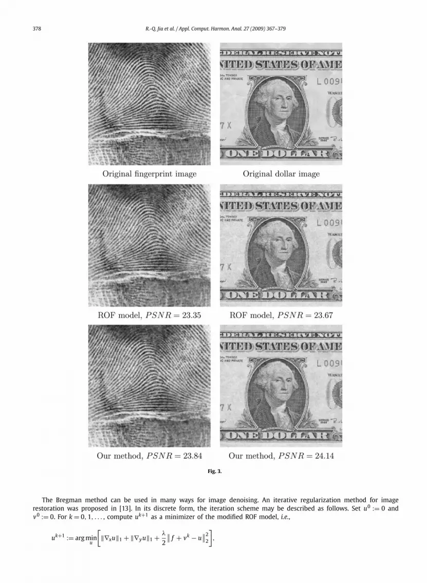
We test our algorithm on three representative images: Barbara, Fingerprint, and Dollar. Suppose that the gray-scale ofan original image is in the range between 0 and 255. A Gaussian noise with normal distribution N(0, σ 2) is added to theoriginal image. We choose σ = 25. The peak-signal to noise ratio (PSNR) of each noised image is about 20.14. We compareour results with the pure shrinkage method via wavelet decomposition and wavelet packet decomposition, and the ROF


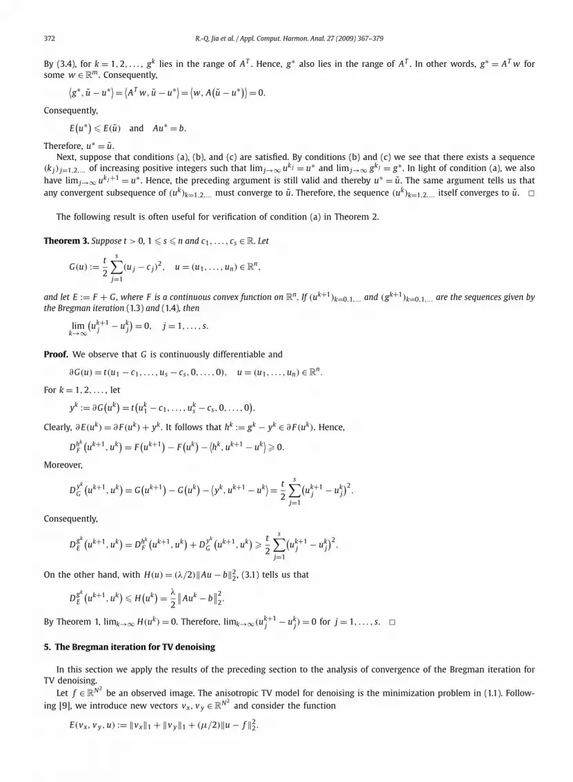
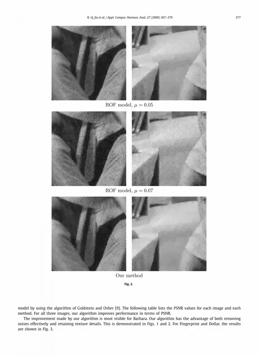
Fig. 2.

model by using the algorithm of Goldstein and Osher [9]. The following table lists the PSNR values for each image and eachmethod. For all three images, our algorithm improves performance in terms of PSNR.

The improvement made by our algorithm is most visible for Barbara. Our algorithm has the advantage of both removingnoises effectively and retaining texture details. This is demonstrated in Figs. 1 and 2. For Fingerprint and Dollar, the resultsare shown in Fig. 3.


Fig. 3.

The Bregman method can be used in many ways for image denoising. An iterative regularization method for imagerestoration was proposed in [13]. In its discrete form, the iteration scheme may be described as follows. Set u0 := 0 andv0 := 0. For k = 0,1, . . . , compute uk+1 as a minimizer of the modified ROF model, i.e.,

uk+1 := arg minu

[‖∇xu‖1 + ‖∇yu‖1 + λ∥∥ f + vk − u

∥∥22

],

2


Image Wavelet shrinkage Packet shrinkage ROF model Our method

Barbara 25.37 25.00 25.78 26.66Fingerprint 22.86 22.89 23.35 23.84Dollar 23.31 22.36 23.67 24.14

where 0 < λ < μ, and update vk+1 := vk + f − uk+1. Then the stopping criterion ‖uk − f ‖2 � δ is used, where δ representsthe noise level. This scheme may be considered as a multi-step ROF model. The idea is to catch more signal than noise ineach step until it is no longer possible.

Our algorithm can be viewed as a two-step ROF model. The approximate image g obtained in the first step containsmost of the signal and removes most of the noise. However, the residual v = f − g still contains some parts of the signal.In the second step, by using a combination of the Bregman method and wavelet packet decomposition, we can effectivelycatch some parts of the signal. In other words, in these two steps, we try to separate the signal from the noise. This isrelated to the work in [15] for separating images into texture and piecewise smooth parts.

Many researchers have studied image denoising in the wavelet domain. Chan and Zhou [4] did research on combiningwavelets with variational and PDE methods. Chui and Wang [5] investigated wavelet-based minimal-energy approach toimage restoration. When the total energy functional is formulated in the wavelet domain, it was proved in [5, Theorems 4and 5] that the minimization problem reduces to soft or hard shrinkage. In [19] Xu and Osher applied the iterative reg-ularization method in [13] to wavelet shrinkage. Clearly, the methods used in both [5] and [19] were wavelet shrinkages.In comparison, we applied the Bregman method to each subimage obtained from wavelet packet decomposition. Thus, ouralgorithm is different from the aforementioned schemes.

Denoising for texture rich images has been studied extensively in the literature. For example, Gilboa and Osher in [8]investigated semi-local and nonlocal variational minimizations for denoising. It would be interesting to incorporate thetechnique discussed in this paper to the more advanced study as in [8]. This will be topics of future research.

Acknowledgments

The authors are grateful to Dr. Zuowei Shen for his invitation to the research program on Mathematical Imaging andDigital Media held in Singapore between May 5 and Jun 27, 2008. They are pleased to acknowledge the support receivedfrom the Institute for Mathematical Sciences at the National University of Singapore during the research program includingthe summer school and the workshops. The authors also sincerely thank Cai, Osher, and Shen for making the two papers[2] and [3] available to them.

This research work was partially supported by NSERC Canada under Grant OGP 121336.

References

[1] L. Bregman, The relaxation method of finding the common points of convex sets and its application to the solution of problems in convex optimization,USSR Comput. Math. Math. Phys. 7 (1967) 200–217.

[2] J.F. Cai, S. Osher, Z.W. Shen, Linearized Bregman iterations for compressed sensing, Math. Comput., in press.[3] J.F. Cai, S. Osher, Z.W. Shen, Convergence of the linearized Bregman iteration for �1-norm minimization, Math. Comput., in press.[4] T.F. Chan, H.M. Zhou, Total variation minimizing wavelet coefficients for image compression and denoising, in: Proceedings of International Conference

on Image Processing, vol. 2, IEEE, 2001, pp. 391–394.[5] C.K. Chui, J.Z. Wang, Wavelet-based minimal-energy approach to image restoration, Appl. Comput. Harmon. Anal. 23 (2007) 114–130.[6] A. Cohen, I. Daubechies, P. Vial, Wavelets and fast wavelet transforms on an interval, Appl. Comput. Harmon. Anal. 1 (1993) 54–81.[7] D.L. Donoho, I.M. Johnstone, Minimax estimation via wavelet shrinkage, Ann. Statist. 26 (1998) 879–921.[8] G. Gilboa, S. Osher, Nonlocal linear image regularization and supervised segmentation, Multiscale Model. Simul. 6 (2007) 595–630.[9] T. Goldstein, S. Osher, The split Bregman method for L1 regularized problems, UCLA CAM Report (08-29).

[10] R.A. Horn, C.R. Johnson, Topics in Matrix Analysis, Cambridge University Press, Cambridge, 1991.[11] R.Q. Jia, The projection method in the development of wavelet bases, in: Lizhen Ji, Kefeng Liu, Lo Yang, Shing-Tung Yau (Eds.), Proceedings of the

Fourth International Congress of Chinese Mathematicians, vol. 1, Higher Education Press, Beijing, 2007, pp. 576–597.[12] Y. Meyer, Oscillating Patterns in Image Processing and Nonlinear Evolution Equations, Univ. Lecture Ser., vol. 22, Amer. Math. Soc., Providence, 2001.[13] S. Osher, M. Burger, D. Goldfarb, J.J. Xu, W.T. Yin, An iterative regularization method for total variation-based image restoration, Multiscale Model.

Simul. 4 (2005) 460–489.[14] L. Rudin, S. Osher, E. Fatemi, Nonlinear total variation based noise removal algorithms, Phys. D 60 (1992) 259–268.[15] J.-L. Starck, M. Elad, D.L. Donoho, Image Decomposition via the combination of sparse representations and a variational approach, IEEE Trans. Image

Process. 14 (2005) 1570–1582.[16] G. Strang, T. Nguyen, Wavelets and Filter Banks, Wellesley–Cambridge Press, Wellesley, MA, 1997.[17] Y. Wang, W. Yin, Y. Zhang, A fast algorithm for image deblurring with total variation regularization, CAAM Technical Report TR07-10, Department of

Computational and Applied Mathematics, Rice University, Houston, Texas 77005, June 2007.[18] M.V. Wickerhauser, Adapted Wavelet Analysis from Theory to Software, A.K. Peters, Wellesley, MA, 1994.[19] J.J. Xu, S. Osher, Iterative regularization and nonlinear inverse scale space applied to wavelet-based denoising, IEEE Trans. Image Process. 16 (2007)

534–544.[20] W.T. Yin, S. Osher, D. Goldfarb, J. Darbon, Bregman iterative algorithms for �1-minimization with applications to compressed sensing, SIAM J. Imaging

Sci. 1 (2008) 143–168.

Documents

Convergence analysis of the Bregman method for the variational model of image denoising