Embed Size (px)
Citation preview
Robust bus-stop identification and denoisingmethodology
Fabio PinelliIBM-Research Ireland
Email: [email protected]
Francesco CalabreseIBM-Research Ireland
Email: [email protected]
Eric BouilletIBM-Research Ireland
Email: [email protected]
Abstract—The analysis of public transportation data is re-ceiving an increasing amount of attention from the researchcommunity in the past few years. This interest is fueled by thewidespread installation and open access to a variety of sensortechnologies for collecting data on the state of the transportsystem in many cities around the world. Different cities providedifferent data sources and in many cases the only commondataset is represented by GPS data of the vehicle fleet. Veryoften, the data contain erroneous or missing information thatshould be corrected before proceeding with their analysis. Inthis paper, we propose a methodology to de-noise scheduledbus stops and detect time schedule information using GPS AVLdata. The methodology performs different sequential steps: i)cleaning process and detection of trips; ii) bus stop extraction;ii) bus stop clustering; iv) feature extraction; v) classificationmodel construction and application. Moreover, the impact on thewhole process of different methods applied in different steps isempirically evaluated on datasets with different temporal extent.
I. INTRODUCTION
The rapid growth of demand for transportation and highlevels of car dependency has resulted in severe traffic con-gestion in many cities worldwide. The general consensus isthat congestion reduction efforts are better invested in publictransport infrastructure, and in the deployment of IntelligenceTransportation Systems (ITS) for public transits. IntelligentTransportation Systems is an umbrella term encompassingsensor, communications and computing technologies to man-age existing infrastructure and transportation systems moreefficiently, and hence contribute to the reduction of congestion.ITS systems extracts Key Performance Indicators (KPI), suchas Estimated Times of Arrival (ETA), from real time locationtracking and traffic monitoring technologies like GPS, induc-tion loops, video cameras and other opportunistic sources ofinformation. Initially public transport KPIs were used mainlyby the operator in making informed decisions to improvetheir service operations. Today, realtime KPIs are also beingused in smartphone travel applications that help the travelercircumvent traffic disruptions and navigate the public transitnetwork seamlessly. This kind of application often requiresgeospatial information about the location of the public transitconnection, and the road network between the connections.This information is often maintained by different entities, thusnot always consistent, it is often outdated, and it is oftencorrupted with some amount of errors or noise.
In this paper we address this issue and introduce a newmethodology for detecting the correct location of bus stopsand consequently extract an accurate time schedule fromhistorical digital traces. We describe a technical solutionsfor de-noising general scheduled transportation data. We thenprovide a robust solution for filtering out incorrect informationas well as adding missing information regarding the publictransportation systems. The method requires historical digitaltraces consisting of locations and optionally timestamps ofeach vehicle of a transit fleet. Like other data sources, thedigital traces can be sparse with a low sampling rate, and it canbe corrupted with errors or noise. The method adopts a multi-steps process that includes different data mining, statistical andmachine learning techniques to perform analysis and classi-fication of spatiotemporal data and static road information.This multi-step process consists of: (1) a cleaning processplus a clustering algorithm on positioning data to obtain asuperset of potential vehicle stops; (2) the computation of afeatures set from an output subset of the clustering and theconstruction of classifier using a partial ground truth; and (3)the application of the classification model to the remainingoutput set of potential stops. The classified stops can be thenmapped on the street network and together with digital tracesthey are used to de-noise other transportation data such asroad network, time schedule, and road shapes, by adding,removing, or correcting the data. Throughout this processthe proposed method includes a notion of confidence in theclassification results. This additional information allows theuser to rank the corrections by confidence levels, visuallyinspect the lowest ranked corrections, and manually performadditional corrections if necessary.
Furthermore, for each step of the process we investigatethrough a case study different possible solutions and, thus, weevaluate their impact on the results justifying one choice w.r.t.to the others. In this case study we adopt three datasets withdifferent temporal extent in order to study if the methodologyis influenced by the size of the dataset.
The rest of the paper is organised as following: in Sec. II weprovide an overview of existing works regarding the analysisof digital traces, extraction of KPIs for transport systems andthe extraction of infrastructure data. In Sec. III, we describe theproposed bus stop detection process that will be evaluated ona case study in Sec. IV. In this last section, we also producea comparison between different approaches discussing their
positive and negative impacts on the process. In Sec. V, weremark and highlight the innovative aspects of the proposedmethodology and its improvable points. Conclusions and fu-ture works are finally discussed in Sec. VI.
II. RELATED WORK
The proposed methodology deals with the analysis tracesof mobile objects, in this section we discuss existing worksrelated to this area. In particular, we focus on works con-cerning the extraction of spatio-temporal pattern from digitaltraces, then we will discuss papers investigating IntelligentTransportation Systems for public transits and finally, we willpresent approaches related to the extraction of infrastructuredata. Several papers deal with the extraction of spatio-temporalpatterns from trajectory data. In [9], the authors propose a newmethod for mining sequences of frequent regions together withtypical transition times. In [11], the authors define a clusteringmethod aimed at extracting groups of similar trajectories basedon different definition of the distance between two traces ofobjects. Following the research line of mobility mining [7],a new environment for mining and analysing trajectories ofmobile object has been defined and described in [8] wherethere is a considerable analysis of the urban mobility throughthe definition of new data mining algorithms tailored to GPStraces. Another example of analysis GPS traces has beencarried out in [16], [15] where the authors define severalalgorithms to mine trajectory data and their final goal is tobuild a web platform where users can share their mobilityexperience and receive back recommendations.
Other works, instead, are focused on the analysis of GSMtraces, as in [2], [3] where the authors studied GSM datain order to describe and interpret the urban environment andhow the people live the cities. Another interesting work is[14] which not only defines a new methodology to extractmobility profiles of users, but also compares the results ofGPS and GSM data in the context of a car pooling applicationshowing that the former provides a greater level of accuracybut, under some circumstances, also the latter can be a suitabledata source.
Several works propose Intelligent Transportation Systemsfor public transit, as, for example, in [6], where the authorsintroduced an innovative platform in order to provide real-time analysis of the bus transportation system by meansof the extraction of several KPIs. In the same context, theauthors of [13] propose a new methodology to estimate thetime of arrival of buses at next stops by means of a kernelregression algorithm. In both papers, the authors assume thatthey are dealing with correct infrastructure data, and they donot propose or use any further methods to correct such datasources, even if their approaches require precise system data.
A considerable research production is already dealing withdefinition of algorithms and methods to extract infrastruc-ture data (e.g. network data, locations of bus stops and soon) from a dataset of trajectories. For example, in [12] theauthors, through several trajectory clustering steps, estimatethe location of bus stops for then studying the changes of
the accessibility in different time of the day in the city ofRome. The authors do not test their results regarding theestimation of the location of bus stops with the ground truth.Instead, in this work, we propose a new process to generatean accurate set of bus stops by means of different data miningalgorithms such as clustering and classification. On a differentapplication scenario, [4] presents a method for automaticallyconverting raw GPS traces from everyday vehicles into aroutable road network. The method begins by smoothing rawGPS traces using a novel aggregation technique. After thetraces are moved in response to the potential fields, they tendto coalesce into smooth paths. The aim of [1] is the extractionof the different components of a public transit system usingGPS traces: location of bus stops, route shapes, and schedule.Concerning the detection of bus stops, the authors define amethodology based on kernel density estimation. They thencompare all the stops they generate with the ground truthverifying that, in general, their method is able to find allthe scheduled bus stops, but it also detect false negative, i.e.stops that are not real bus stops and do not provide a directway to distinguish ones from anothers. Our method, instead,classifies scheduled and not-scheduled stops with, in general,a great precision based on some set of spatiotemporal features.Moreover, we deal with a city scale system while in [1] theyanalyse the traces of campus buses.
III. PROCESS DESCRIPTION
In this section, we describe the methodology adopted toaccurately detect locations of scheduled stops. The processis built to create a classifier able to separate scheduled stopsfrom the others based on a set of features. Before describingeach step of the process, it is necessary to introduce a clearterminology:
Scheduled stop A point where vehicles are planned to stopby, such as all the stops which are included in the time table;Unscheduled stop A point where the vehicles are notexpected to stop, but where stops are nevertheless observedwith a high frequency. This set may include traffic lights,traffic congestions and so on;Potential stop A point not yet classified as scheduled orunscheduled stop, e.g. this can be either a scheduled stop ora traffic light;Bus line A bus line is a sequence of scheduled stops;Trajectory A trajectory is the set of GPS points observedat regular intervals from each single vehicle. Notice that avehicle can serve different bus lines, and can send its locationeven if it is traveling off route;Journey A journey is a segment of vehicle trajectory whichcovers the sequence of all the scheduled stops contained in abus line.
The entire process is shown in Figure 1. Three main stepsare part of the whole process: one for the detection ofpotential bus stops, one for the extraction of spatiotemporalfeatures and the construction of a classifier, and lastly the

Historicaldata
Cleaning
Stop Generation
Clustering
Stop detection
Generation of Features
Classification model
Features selection and
Classification model
Potential bus stops
Partial ground
truth
EvaluationTraining set
Classification model
Application of theclassification model
Historicaldata
(test set)
Detected Bus stops
Fig. 1. The figure shows the architecture of the entire process, the steps and necessary input datasets.
application of the classifier to historical data to correctly labelscheduled and unscheduled stops. Notice also that the entiremethodology requires historical data but also a partial groundtruth regarding the correct location of the bus stops for someof the bus lines under analysis.Stop detection: The first step of the process is detection of aset of potential stops received in the input raw historical data.This is composed by three sub-steps to be applied to the dataof a single bus line: first split the trajectories of each vehicleinto journeys and remove invalid points; second extract all thepoints where a bus performs a stop, third apply a clusteringmethod over this dataset of potential bus stops. In orderto remove invalid points we use spatiotemporal thresholdsidentifying, thus, points too far or with not-realistic speeds.Moreover, this cleaning phase is necessary to split the entiretrajectory of a vehicle (i.e. all the GPS observations relative toa single vehicle) in a set of journeys and then associate eachof them to the relative bus line. The second sub-step is thedetection of the stops along each single journey performedby each vehicle. Two methods are separately evaluated anddiscussed in Sec. IV. The last sub-step is based on theassumption that buses performing the same bus line typicallystop in similar locations, so that the application of clusteringmethod represent the easier way to group together potentialstops sharing a similar typology, i.e. scheduled stops canbe grouped together as well as stops at traffic lights can begrouped together and so on. Two different kinds of clusteringmethods are applied and then discussed in Sec. IV. Notice,again, that the stop detection step is performed for a singleline at the time, i.e. we select all the journeys related to acertain bus line, performed also by different vehicles, and weextract the set of potential bus stops from these journeys. Wewant to remark that this set of potential bus stops includesboth scheduled and unscheduled stops, i.e. traffic lights,traffic congestion and so on.
Feature selection and classification model: This step ofthe process receives as input the set of potential bus stops,generated during the former step, and a partial ground truth,i.e. the correct location of the bus stops for one or more buslines. Two subtasks compose this step of the process, oneis necessary to extract interesting spatiotemporal features todescribe the potential stops generated before. This is basedon the assumption that clusters including unscheduled stopor scheduled stop have different spatiotemporal features, i.e.the duration, the density, the shape of stops performed in theproximity of a traffic light are different to the one relatedto a real bus stop. The extraction of these features allowsus to detect such differences and use them on a classifier.Indeed, the construction of the classifier represents the secondsubtask of the Feature selection and classification model
step, it receives in input the set of potential bus stops withtheir features and each of them is labelled as scheduled orunscheduled based on its distance to the closest real bus stop.This dataset is used as training set to build a classifier. Theoutput of this sub-step is the classifier itself.
Application of classification model: The application of theclassification model to the remaining potential bus stopsreferring to the rest of bus lines composing the transportationsystem is the last step the the process. Considering the factthat, in most of the case, scheduled bus stops, and not, sharethe same properties among bus lines, thus the application ofthe classifier built during the previous step to the remainingpotential bus stops is the natural way to correctly estimatescheduled and unscheduled bus stops for the entire system.
Notice that the application of the process can return differentresults if the intermediate steps are not performed correctly. Inparticular, the choice of the most suitable clustering algorithm,or the suitable classifier can give different and, sometime, un-expected and undesired results. All the steps will be evaluated

through a case study performed on real bus data, a comparisonof different approaches is furnished and evaluated in terms ofaccuracy of the results.
IV. CASE STUDY
In this section we describe the application of the busstop detection process to three real datasets of GPS traces.Moreover, each step introduced in Sec. III is discussed andanalysed in order to empirically justify the different choiceswe made and their influence on the overall results.
A. Datasets
The datasets we used for the application of the bus stopdetection process are collected by the bus operator in Dublin,Ireland1. We used three datasets with a dissimilar time extentin order to evaluate the impact of the amount of data oneach phase of the overall process. In Table I, we report themain features of each analysed datasets in terms of numberof points, vehicles and bus lines. We remark, also, that thetypical sample rate for all the dataset is around 20 seconds.
Statistics 1 week 2 weeks 1 monthN. of points 11,467,141 23,074,967 37,885,186
N. of vehicles 951 972 976N. of lines 511 514 520
TABLE ITHE TABLE CONTAINS THE RELEVANT STATISTICS TO DESCRIBE THE
DIFFERENCES AMONG THE DATASETS UTILISED FOR THE APPLICATION OF
THE BUS STOP DETECTION PROCESS.
B. Stop detection
As described in the previous section, the stop detection steprequires, first of all, a procedure to remove invalid points fromthe dataset under analysis. In order to solve this issue, we useda spatial threshold to remove points that are too far apart, and aspeed threshold to detect sequence of points that translate intobus speeds that are too unrealistic for a urban environment. Weset these thresholds to respectively 1000 meters and 70 km/h.Notice that this does not remove the points not associated withany routes.
The trajectory described by a single vehicle can coverseveral journey on the same bus line as well as several journeysof different bus lines. Thus, it is important to identify thedifferent journeys associated with a specific bus line performedby a single vehicle. Moreover, splitting the initial trajectoryin a set of journey allows us to remove points describingmovements of busses that are off route. The data set usedin this case study includes a bus line attribute that identifiesthe bus line served by the bus. In some cases we observeinconsistencies between the value of the bus line attribute andthe actual positions of the bus. This happens when a bus hasended a journey and is on its route to the depot or to thenext journey. In our case the inconsistencies are statisticallyinsignificant and are safely ignored by our method. If on the
1http://www.dublinbus.ie
53.33
53.34
53.35
53.36
53.37
53.38
53.39
53.4
53.41
53.42
53.43
-6.5 -6.45 -6.4 -6.35 -6.3 -6.25 -6.2
(a) Raw data of the bus line 38 be-fore the cleaning procedure
53.33
53.34
53.35
53.36
53.37
53.38
53.39
53.4
53.41
53.42
53.43
-6.44 -6.42 -6.4 -6.38 -6.36 -6.34 -6.32 -6.3 -6.28 -6.26 -6.24
(b) Journeys of the bus line 38 afterthe cleaning procedure
Fig. 2. The results of the cleaning process on the raw data of the bus line38
other hand the bus line attribute is not available, or if it cannotbe trusted, an intermediate step would be required to infer theassociation between the vehicle and a bus line directly from theraw input data. The research literature abounds with solutionsto solve this association (see [12] for a list of references),and it is thus not discussed in this paper. In order to dividethe initial trajectory of a vehicle into a set of journeys foreach bus line, we subdivide each individual vehicle trajectoryinto one or more sub-trajectories according to the value ofits bus line attribute. The results of this association are thenparsed in order to identify single journeys. To accomplish thistask, we used a temporal threshold: if the temporal distancebetween two consecutive points pt and pt+1 is larger than 900seconds the algorithm considers pt as the end of a journeyand pt+1 at the beginning of the next one. An example of thecleaning process is reported in Figure 2 for a given bus line.Figure 2(a) shows an example of several vehicle trajectoriesobserved over a one week period associated with the bus line.Figure 2(b) illustrates the output of the cleaning process afterremoving odd straight lines and invalid points, thus resulting inan accurate separation between the different vehicle journeysrelated to that bus line.
At this point of the process, all the journeys are associatedwith the relative bus line. The next step, aiming at detectinglocation where the vehicles stops, analysises all the journeysfor a given bus line at the time. We implement two differentmethods to detect stop location of vehicles. The first one isbased on spatiotemporal thresholds, such as if a set of pointsof a vehicle falls in a area of a given radius (spatial thresholdthstop
spatial) and the total duration is smaller than the temporal
threshold (thstoptemporal), then this set is considered as a stop. A
formal definition of these stops is defined as follow:
Definition 1: Given a journey J of a bus on a bus lineand the thresholds thstop
spatial and thstoptemporal, a stop is defined
as the centroid P of the maximal subsequence S of Jwhere the points remain within a spatial area for a certainperiod of time: P = centroid(S) where S is defined as:S = ⟨pm . . . pk⟩ |0 < m ≤ k ≤ n ∧ ∀m≤i≤kDist(pm, pi) ≤thstop
spatial ∧Dur(pm, pk) ≥ thstoptemporal.
where Dist is the geographical distance between two points,and Dur is the temporal difference between two points.
Time
Posi
tion
Detected stop
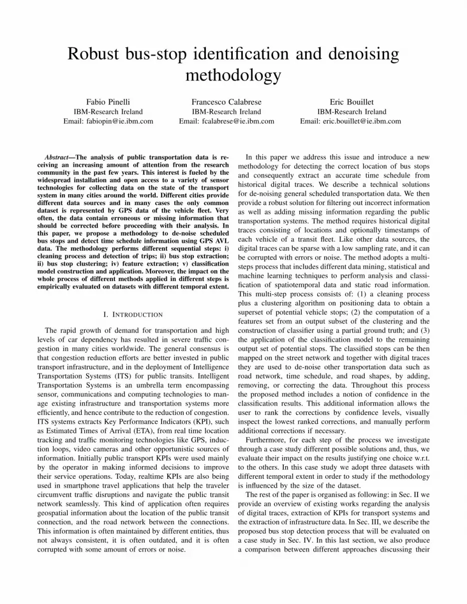
(a) An example of the detec-tion of stops using spatiotempo-ral thresholds
0
10
20
30
40
50
60
70
80
0 20 40 60 80 100 120 140 160
Spee
d�(k
m/h
)
Time
(b) An example of the detection ofstops using the speed-based method
Fig. 3. Examples of the two used methods for the stop detection.
Since at this stage of the process, we do not want to loseany kind of stop, and we want to generate as much as possiblepotential bus stops, the described solution might not be themost suitable for our purposes since some cases cannot bedetected, e.g. when a bus overcomes a scheduled stop withoutstopping, a traffic light showing green light. An example ofthe stop detection methodology is described in Figure 3(a)
For these reasons, we develop another method to detect thestops, and it is speed-based, such as it considers the currentspeed of the bus, and a stop is detected if the derivative of thespeed (acceleration) switches from negative to positive. In thefollowing the definition of this kind of stops:
Definition 2: Given a journey J of a bus on a bus line, astop is defined as the point P which is the last point of consec-utive points with a negative value of derivative of the speed.P = last(S) where S is defined as: S = ⟨pm . . . pk⟩ |0 <m ≤ k ≤ n ∧ ∀m≤i≤k(Speed(pi − Speed(pi−1) ≤ 0.
Moreover, in Figure 3(b) we show the trend of the speed for aselected journey (blue line), and we also represent what stopsare considered as stop point according to Definition 2. We caneasily notice that all the stop points represent the local minimaof the speed trend, as implicitly contained in Definition 2. InTable II we report the number of stops we detect consideringall the journey related to a given bus line, in this case the busline n. 38.
Method 1 week 2 weeks 1 monthN. of stops with Method 1 1879 3628 5988N. of stops with Method 2 11844 23562 39049
TABLE IITHE TABLE CONTAINS THE NUMBER OF STOPS DETECTED ANALYSING
ALL THE JOURNEYS OF THE BUS LINE 38.
As we can see the most suitable method between the twopreviously introduced is the second. Indeed, in all the cases thesecond method based on the speed generates a greater numberof stops overcoming, thus, the limitations of the first method.Taking as example the bus which skips a stop, even if noneof the passenger requests to stop, the driver has to reduce thespeed in order to verify if someone wants to get in, and thiscase is captured using the second method and not with the
first. Moreover, the second procedure is parameter free andthis makes it again more appropriate than the first one.
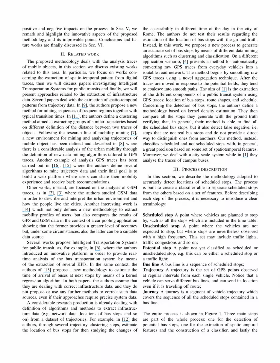
Figure 4(a) shows the stop points detected with firstmethod, it is possible to notice that zones where we detect fewstops. This, clearly, can influence the results of the next steps.Moreover, Figure 4(b) presents a different scenario where theline is all covered by the set of detected stops. Notice thatfor the rest of the case study experiments we use the datasetsgenerated by means of the speed-based method.
53.33
53.34
53.35
53.36
53.37
53.38
53.39
53.4
53.41
53.42
53.43
-6.44 -6.42 -6.4 -6.38 -6.36 -6.34 -6.32 -6.3 -6.28 -6.26 -6.24
(a) Stops detected for the bus line 38by means of spatiotemporal thresh-olds
53.33
53.34
53.35
53.36
53.37
53.38
53.39
53.4
53.41
53.42
53.43
-6.44 -6.42 -6.4 -6.38 -6.36 -6.34 -6.32 -6.3 -6.28 -6.26 -6.24
(b) Stops detected for the bus line 38considering the trend of the speed
Fig. 4. Sample of bus stops detected with two different methods
All the journeys related to a specific bus lines share theroute to travel through, this also means that they sharealmost all the stop, scheduled and unscheduled. Indeed,along the same route the vehicles have to stop at the samescheduled stops, but also they encounter the same trafficlights, stop signals, and so on. However, the observations ofsuch common locations can be displaced for several reasonsand handling a large number of potential stops to learn aclassifier may not be suitable. For all these reasons, theapplication of a clustering algorithm is necessary, in order tosolve two different issues: i) remove the noise, such as stoppoints shared among few buses – low frequency bus stops;ii) group together points representing the same location, e.g.one stop point refers to the beginning of the bus stop area,and another, instead points to the end of the same bus stoparea: these two points have to be grouped together since theyrepresent the same bus stop. In this section, we investigatethe usage of two clustering methods:
K-MEANS [10] This well-known method of clustering aimsto partition the n observations of the initial data into k clusters– input parameter – in which each observation belongs tothe cluster with the nearest mean. K-MEANS has two maindrawbacks, the choice of the correct parameter k, and the factthat it is not very robust to noise. However, a set of k clusteris always returned.DBSCAN (density-based spatial clustering of applicationswith noise) [5] is a density-based clustering method. it finds anumber of clusters starting from the estimated density distri-bution of corresponding nodes. DBSCAN requires two inputparameters: ϵ and min points, the first one represents a radiusin within the algorithm searches of ϵ-neighbours points, thesecond one indicates the minimum number of points to forma cluster. Moreover, DBSCAN returns also a cluster called

noise, containing all the points discarded during the clusteringprocedure. The main drawback of DBSCAN is the choice ofthe two parameters, this is not always straightforward, and inthe following we experimentally demonstrate the influence ofthat choice on the results.
Moreover, we measure the performance of the two approachesby means of the Precision and the Recall measures. Weremember that the Precision is defined as the fraction ofdetected bus stops that were labeled as true bus stops w.r.tthe total number of detected bus stops, and the Recall is thefraction of correctly detected stops w.r.t. the total number ofground truth bus stops. Before discussing the results obtained,let us clarify the method used to evaluate the obtained clustersw.r.t. the location of the real bus stops. We take the location ofthe real bus stops, i.e. ground truth, then we define a dynamicspatial threshold τ based on the distance between a real stopand its previous stop and its next stop (i.e. we take into accountthe fact that in urban areas the stops are closer than ruralareas). A potential stop is labeled with true if its distance withthe closest real stop is less than τ , andfalse otherwise. Notice,also, that the location of some bus stops is not correct, thus thisthreshold allows us to correctly label the clusters even if thelocation of their centroid does not match to one of the relativebus stop. Furthermore, we study if the size of the datasetsinfluences the results of the clustering algorithms.
1) K-means: In this section, we investigate the resultsobtained using the K-MEANS algorithm. Firstly, we discusshow we set up the initial number of cluster k. Considering thefact that the goal of this process is to get a larger number ofpotential bus stops than the exact number of scheduled stopsdesigned for a given bus line, we set up the parameter k asa multiple of the scheduled stops. Moreover, we select theinitial k points in this way: the first point corresponds to thefirst k, and, until we do not reach k points, we select the pointsthat are at least 100 meters from others points following thedirection described by the bus line.
In Figure 5, we report the results of the analysis of Precisionand Recall values. We can highlight two main aspects from thisfigure. First, the Recall – that, in this application, representsthe main feature to compare different clustering algorithms –is always high but it does not reach the 100%, meaning thatthe generated clusters do not cover all the stops designed forthe given bus line. The second interesting aspect to notice isthat the performance of the algorithm are not influenced by thesize of the dataset, except for one bus line (38 outgoing). Ingeneral, the value of the Recall decreases with the increase ofthe size of the dataset. The fact that K-MEANS is not handlingthe noise can effect the Recall measure. Indeed, it is possiblethat noisy points shift away the mean of the clusters w.r.t. thelocation of real bus stops. Additionally, having a considerablehigh value of the precision means that the generated datasetof potential bus stops contains an appreciable number ofunscheduled stops, and thus it contains both type of stops:scheduled and unscheduled.
40
50
60
70
80
90
100
110
1 week 2 weeks 1 month
Per
centa
ge
Dataset
00380001 Recall00380001 Precision
00381001 Recall00381001 Precision
038A001 Recall038A0001 Precision
038A101 Recall038A1001 Precision
Fig. 5. The graph shows the Precision and Recall values for the K-MEANSalgorithm applied to 4 bus lines on the three different datasets.
2) DBSCAN: As previously discussed DBSCAN needs twoinput parameters: a spatial radius ϵ and the minimum numberof points min pts. The choice of these parameters is crucial inorder to obtain suitable number of clusters. The ϵ parametersrepresents the spatial radius of the area in which the algorithmsearches ϵ-neighbour points. For this parameter we selectvalues that represent a reasonable significance in this context,i.e. 10, 20 and 50 meters. The min pts parameters representsthe minimum number of points that are required to createa cluster. This has been set up equal to a proportion of thenumber of journeys associated with a specific bus line. In theexperiments we used 10, 15, 20, 30.
In Figure 6 we report the number of clusters obtained withdifferent configurations for the input parameters of DBSCAN. In Figure 6(a) we evaluate the influence of min ptsparameter. The effects ϵ are, instead, shown on Figure 6(b).We can notice that for small values of ϵ, i.e. the radius usedduring the DBSCAN computation to verify the density, thenumber of clusters decreases drastically. These configurationsof the parameters generate useless results for the next step ofthe process. Indeed, the goal of the application of the clusteringalgorithm is to obtain a large set of potential bus stops whichincludes the real bus stops but also the unscheduled ones. Thenext classification step will distinguish the two types based ona set of spatiotemporal features.
50
100
150
200
250
300
10 15 20 25 30
N.�o
f�clu
ster
s
N.�of�minimum�points
eps=10eps=20eps=50
(a) The influence of the min ptsparameter to the number of extractedclusters
50
100
150
200
250
300
10 15 20 25 30 35 40 45 50
N.�o
f�Clu
ster
s
Epsilon�(meters)
MinPts=10MinPts=15MinPts=20MinPts=30
(b) The influence of the ϵ parameterto the number of extracted clusters
Fig. 6. How min pts and ϵ influence the number of cluster returned byDBSCAN .
As already analysed for the application of the K-MEANS, we investigate the values of the Precision and Recall for

the obtained clusters by means of DBSCAN . We rememberthat a high value of the Recall measure means that the datasetcontains a high percentage of the real bus stops. On the otherhand, the Precision measures which percentage of the gener-ated potential bus stops is covered by the real bus stops, thus,a low value of Precision means that the clustering algorithmhas generated a large number of unscheduled stops. Noticethat the most suitable dataset for the proposed methodologyis the one which has a high (100%) Recall and a low valueof Precision.
0
20
40
60
80
100
50 100 150 200 250 300 350
Per
centa
ge
N.�of�clusters
Recall 00380001Precision 00380001
Recall 00381001Precision 00381001
0
20
40
60
80
100
50 100 150 200 250 300
Per
centa
ge
N.�of�clusters
Recall 00380001Precision 00380001
Recall 00381001Precision 00381001
0
20
40
60
80
100
0 50 100 150 200 250 300
Per
centa
ge
N.�of�clusters
Recall 00380001Precision 00380001
Recall 00381001Precision 00381001
Fig. 7. The precision and Recall trends obtained applying DBSCAN to thedifferent datasets under analysis. On the top left one week, top right two weekand at bottom the one month
As shown in Figure 7, we can notice that the results areconsiderably better using one week of data w.r.t. to the otherdatasets. Indeed, we are able to get 100% of Recall, such as,we are able to detect all the real bus stops for that given busline. Moreover, the figure confirms that the configuration ofthe parameters plays an important role in order to generatedesired results, indeed, in NN cases the performance of thealgorithm degraded significantly.
Let us discuss the results obtained applying the two clus-tering methods. Regarding K-MEANS we can conclude that italways results in a high Recall, however, it does not reach the100%, thus, it generates a set of clusters that does not includeall the real bus stops. Moreover, K-MEANS does not requirea strong effort to set up the initial k parameter. On the otherhand, DBSCAN is able to generate all the real bus stops withthe appropriate parameter configurations, but for some otherinitial values the number of generated clusters is too small toreach a high Recall. Therefore, the choice of the best clusteringalgorithm requires to find a good trade-off between the effortof setting up the input parameters and in obtaining 100% ofRecall. Summarising we can affirm that:
• K-MEANS shows always a high recall;• The presence of noise data influences the performance of
K-MEANS ;• DBSCAN is very sensitive to the input parameters;• DBSCAN can have higher Recall than K-MEANS and it
can reach the 100%;
53.33
53.34
53.35
53.36
53.37
53.38
53.39
53.4
53.41
53.42
53.43
-6.44 -6.42 -6.4 -6.38 -6.36 -6.34 -6.32 -6.3 -6.28 -6.26 -6.24
1week kmeansreal bus stops
53.33
53.34
53.35
53.36
53.37
53.38
53.39
53.4
53.41
53.42
53.43
-6.44 -6.42 -6.4 -6.38 -6.36 -6.34 -6.32 -6.3 -6.28 -6.26 -6.24
1 week dbscanreal bus stops
53.33
53.34
53.35
53.36
53.37
53.38
53.39
53.4
53.41
53.42
53.43
-6.44 -6.42 -6.4 -6.38 -6.36 -6.34 -6.32 -6.3 -6.28 -6.26 -6.24
2 weeks kmeansreal bus stops
53.33
53.34
53.35
53.36
53.37
53.38
53.39
53.4
53.41
53.42
53.43
-6.44 -6.42 -6.4 -6.38 -6.36 -6.34 -6.32 -6.3 -6.28 -6.26 -6.24
2 weeks dbscanreal bus stops
53.33
53.34
53.35
53.36
53.37
53.38
53.39
53.4
53.41
53.42
53.43
-6.44 -6.42 -6.4 -6.38 -6.36 -6.34 -6.32 -6.3 -6.28 -6.26 -6.24
1 month kmeansreal bus stops
53.33
53.34
53.35
53.36
53.37
53.38
53.39
53.4
53.41
53.42
53.43
-6.44 -6.42 -6.4 -6.38 -6.36 -6.34 -6.32 -6.3 -6.28 -6.26 -6.24
1 month dbscanreal bus stops
Fig. 8. A visual comparison between the results obtained on the 3 datasetsby means of the two clustering methods is shown. The left column containsthe results obtained applying KMEANS. The right column, instead, visualisesthe centroids of the DBSCAN clusters. The graphs show also the location ofthe real bus stops for the bus line 38.
• DBSCAN is marginally influenced by noise data.
In Figure 8, we visually compared the results obtainedusing K-MEANS (left column) and DBSCAN (right column)where it is possible to see some differences and commoncharacteristics. The clusters obtained with DBSCAN seemto cover more uniformly the whole shape of the bus line,instead K-MEANS show some almost empty areas as aroundthe coordinates (53.4, -6.37). However, it is possible to seethat both methods extract some potential bus stops between(53.41, -6.44) and (53.42, -6.43). In this area, we discover thepresence of a real bus stop that is not reported on our list ofstops associated with that bus line. Let us highlight that fact fortwo reasons: i) this is a clear case where the proposed methodis useful for, indeed the infrastructure data contain errors ormissing information even if they are provided by the operatoritself; ii) some other bus lines can have similar problems andwe are not aware about that, clearly this influences the resultswe obtained.
Notice that the clusters with Recall 100% obtained by meansof DBSCAN will be used in the next experiments.
C. Feature extraction and classification
Let consider the example reported in Figure 9, where wedepict two different clusters obtained in the previous step, one(top) representing a traffic congestion, and the other (bottom)a cluster close to bus stop. As you can see the two exampleshave different features. For instance the density of the pointsis different, for the cluster in Figure 9(b) representing thebus stop the density of points is much higher. Moreover, the

(a) Stops detected relatively to a traffic congestion
(b) Stops detected relatively to a bus stop
Fig. 9. Two different clusters of stops representing one an example of trafficcongestion (top) and a bus stop (bottom).
shape itself of the clusters is different. In fact, the shape ofthe cluster indicating the traffic congestion, Figure 9(a), islonger and the points are almost uniformly distributed alongthe shape. For these reasons, the next step of the process aimsat extracting different features able to capture the differencesbetween scheduled and unscheduled stops. We consider asrelevant this set of features:
• high: the distance between two points with the lowestand the highest latitude;
• base: the distance between two points with the lowestand the highest longitude;
• area: the product between high and base;• numberOfObjects: the number of points belonging to
the cluster;• density: the ratio between the number of points and the
area;• avgT imeDuration: the time duration of the stop, i.e.
the averaged temporal distance between the first pointand last point that are part of the same detected stop;
• avgSpeed: the average speed measured at the stop;• avgInitSpeed: the speed of the first point considered
as part of the stop (i.e. the first point with a negativeacceleration for the speed-based stop detection method);
• avgEndSpeed: the speed of the last point consideredas part of the stop (i.e. the last point with a negativeacceleration for the speed-based stop detection method);
The first three features describe the spatial shape of thecluster, as described in Figure 9. The numberOfObjectsrepresents the frequency of which this cluster occurs in thedata, most likely the scheduled bus stops have a higher fre-quency. The density merges the previous features considering
that the scheduled bus stops coincide with most dense clusters.The avgT imeDuration is computed as the average timeduration between all the potential stops belonging to thecluster, this feature should identify a different stoppage timebetween scheduled and unscheduled stops. The avgSpeed iscalculated taking into account the average speed observedfor each potential bus stop that is part of the cluster. TheavgInitSpeed averages the initial speed recorded for all firstpoints considered as part of a stop (i.e. the first point witha negative acceleration) which is part of the cluster. Lastly,avgEndSpeed, as for the previous feature, we average thespeeds recorded for all the last point (i.e. the last point witha negative acceleration and notice that it location correspondsto the one associated with the stop itself.) being part of a stopwhich belongs to the cluster.
These extracted features are used to build a classifier whichuses them to categorizes the stops into scheduled and unsched-uled stops. For the classification algorithm we used C5.1 whichis an enhanced version of the C4.5 classifier. This classifieruses the concept of Information entropy, the algorithm choosesone attribute of the data that most effectively splits the samplesinto subsets enriched in one class or the other. Its criterionis the normalized information gain (difference in entropy)that results from choosing an attribute for splitting the data.The attribute with the highest normalized information gainis chosen to make the decision. We used two different testsets, both with the Recall equal to 100% during the clusteringphase, bus line 39 ingoing and bus line 38 outgoing.
The two decision trees have a different depth, 3 and 8respectively. Furthermore, AvgEndSpeed is for both decisiontree the first attribute used for splitting, then Area for theclassifier for the bus line 39, instead density for the 38 ones.
D. Application of the classifier
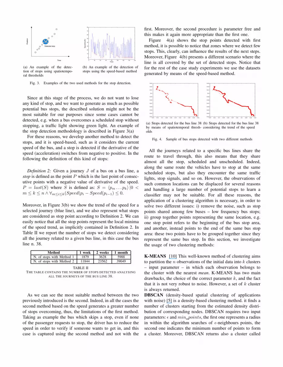
The last step of the process is the application of theclassifier. We use some of the other bus lines as test set of theclassifier evaluating its precision. Figure 10 shows the resultsof the application of two classification models, one built usingthe data of line 39 ingoing, the second one with the data of 38outgoing. We classified the clusters obtained for 6 other lines.We select these 6 lines as a sample of the whole bus linesand we take into account bus lines with different length (i.e.different number of bus stops). The classification results rangefrom 81.25% of precision for the classifier of bus line 39 to thelower 64.45% obtained with the classifier of the bus line 38.In average, the classifier’s precision is around 70%. However,we recall that the locations of some of the bus stops includedin our dataset are wrong, and the list of stops associated withthe bus lines are not always correct, as previously discussed.Both types of errors can affect the results of the classifier.
V. DISCUSSION
In this section, we provide a discussion regarding thepositive and ameliorable aspects of the proposed methodology.
Intelligence Transportation Systems (ITS) for public transitsoften require geospatial information about the location of the
0
20
40
60
80
100
01220001
01200001
00390002
00010001
00380002
038B0001
Pre
cisi
on
�(%)
Results
0039100100380001
Fig. 10. The precision of two models built with bus line 38 outgoing and39 ingoing.
public transit connection, and the road network between theconnections. This information is often maintained by differententities, thus not always consistent, it is often outdated, and itis often corrupted with some amount of errors or noise.
Similar errors in the infrastructure data can invalidate theresults of evaluation of KPIs for public transits. For instance, in[13] the authors propose a new method to estimate the time ofarrival of buses at the stops. In order to have a good estimation,the algorithm requires accurate infrastructure data: correctlocation of bus stops as well as an accurate reconstruction ofthe route shapes. In a scenario where these data sources arenot reliable neither the estimations and the analysis providecan be. Having, thus, a simple and affordable methodology toreconstruct infrastructure data becomes crucial. Our proposedmethodology satisfies these requirements. In fact, the bus stopdetection method proposed in this paper is:
• simple: the process requires few input parameters andtheir tuning does not require any specific domain knowl-edge. Moreover, the process is a combination of pre-processing tools and well-known data mining algorithmswhich results are easy to understand;
• affordable: the methodology requires a set of digitaltraces and a partial ground truth. Since the proposedmethodology represents the initial step before the instal-lation of a Intelligent Transportation system, the digitaltraces of the fleet come with the requirements of theoperators. Furthermore, the mandatory ground truth caninterest few bus lines. In addition, the method does notrequire a large amount of data. Indeed, in the case study,we empirically demonstrate that one week of data wasenough to get interesting results;
• modular: the whole process is organised in multi-stepmanner. Each step requires certain data as input andprovides a particular output. Each of these steps can bereplaced with a different method which can furnish betterresults. Also this aspect has been investigated on the casestudy, where we test the use of different methods and wediscuss their positive and negative effects;
• reliable: the method classifies scheduled and unscheduledbus stops based on a set of features. In fact, this methodol-
ogy does not return a set of potential stops which includesthe real stops as all the existing works, but it returns aclassification on real and not-real stops associating a alsoa confidence level. Based on the confidence level, onecan or not correct the other data sources.
However, the proposed method can be improved underseveral aspects making it more:
• accurate: the case study showed interesting results re-garding the classification of the potential bus stops. How-ever, we did not reach high level of precision. This aspectcan be improved in different ways: i) extend/changethe set of features used by the classifier; ii) considerthe features also during the clustering step and thusdefine a new distance function which takes into accountspatial distance but also other interesting features; iii)extend the process with other steps in order to considerother peculiarities of transit systems, e.g. identification ofrural/downtown bus stops, shared bus stops among buslines, etc.;
• scalable: the current design of the process does not takeinto account that buses share among them some of thebus stops. Currently these shared bus stops are evaluatedand classified every time the process analyses the data ofa bus line. In addition, more efficient clustering methodscan be adopted.
• advanced: the methods adopted in each step are simpleand they provide understandable results. However eachcomponent of the process can be replaced with moresophisticated technique that can enhance its usability andthe general performance, e.g. a different classificationalgorithm, a different clustering method and so on.
Finally, the empirical evaluation of the methodology al-lowed us to investigate different possible solutions to differ-ent problems driving us the comprehension of positive andnegative details. Moreover, this proposed methodology canbe part of a larger set of algorithms and tools aimed atproviding correct and de-noised infrastructure data of publictransit systems.
VI. CONCLUSION AND FUTURE WORK
In this paper we present an innovative methodology to detectthe location of the scheduled stops based on spatio-temporalanalysis, data mining and machine learning algorithms. Incomparison with the state-of-the-art, the proposed method isable to accurately classify scheduled and unscheduled stops.These results are useful as support for other applications aimedat extracting KPIs for transportation systems in real-time. Foreach step of the process we described possible approachesand we investigate their positive or negative impact to theresults. The experiments have been conducted on a real casestudy based on GPS traces of buses. The experiments showa great precision of the method, but possible improvementsare feasible. For instance, we select a possible list of featuresuseful for capturing the differences between scheduled andunscheduled stops, but this list is not exhaustive and neither

complete. In future works, we plan to extend this list consid-ering other spatio-temporal features. Moreover, the proposedmethod does not take into account the fact that buses sharebus stops. The implemented method considers one bus line atthe time, while it should also take advantage of the partialsharing of bus stops among bus lines. Furthermore, in thecurrent design the clustering uses only the spatial distance.In future improvements we would like to study the use ofa distance measure which considers others possible featurerelated to each potential stop. In this work, we mainly focus onthe detection of bus stops, but other data sources describing theinfrastructure of a transportation system can be inconsistent,outdated, corrupted and it can contain noise. In future work,we will investigate possible solutions to provide accuratecorrection of the rest of infrastructure data including static anddynamic information such as time table, route shapes etc.
REFERENCES
[1] James Biagioni, Tomas Gerlich, Timothy Merrifield, and Jakob Eriks-son. Easytracker: automatic transit tracking, mapping, and arrival timeprediction using smartphones. In SenSys, pages 68–81, 2011.
[2] F. Calabrese, G. DiLorenzo, L. Liu, and C. Ratti. Estimating Origin-Destination Flows Using Mobile Phone Location Data. IEEE PervasiveComputing, 2011.
[3] F. Calabrese, F. Pereira, G. DiLorenzo, and L. Liu. The geography oftaste: analyzing cell-phone mobility and social events. In Int. Conferenceon Pervasive Computing, 2010.
[4] Lili Cao and John Krumm. From gps traces to a routable road map.In Proceedings of the 17th ACM SIGSPATIAL International Conferenceon Advances in Geographic Information Systems, GIS ’09, pages 3–12,New York, NY, USA, 2009. ACM.
[5] Martin Ester, Hans-Peter Kriegel, Joerg Sander, and Xiaowei Xu.A density-based algorithm for discovering clusters in large spatialdatabases with noise. In Evangelos Simoudis, Jiawei Han, and Us-ama M. Fayyad, editors, Second International Conference on KnowledgeDiscovery and Data Mining, pages 226–231. AAAI Press, 1996.
[6] L. Gasparini, E. Bouillet, F. Calabrese, O. Verscheure, B. O’Brien,and M. O’Donnell. System and Analytics for Continuously AssessingTransport Systems from Sparse and Noisy Observations: Case Study inDublin. In IEEE Intelligent Transportation Systems Conference, 2011.
[7] F. Giannotti and D. Pedreschi. Mobility, data mining and privacy: Avision of convergence. pages 1–11, 2008.
[8] Fosca Giannotti, Mirco Nanni, Dino Pedreschi, Fabio Pinelli, ChiaraRenso, Salvatore Rinzivillo, and Roberto Trasarti. Unveiling the com-plexity of human mobility by querying and mining massive trajectorydata. The VLDB Journal, 20(5):695–719, oct 2011.
[9] Fosca Giannotti, Mirco Nanni, Fabio Pinelli, and Dino Pedreschi.Trajectory pattern mining. In KDD, pages 330–339, 2007.
[10] J. A. Hartigan and M. A. Wong. A K-means clustering algorithm.Applied Statistics, 28:100–108, 1979.
[11] Mirco Nanni and Dino Pedreschi. Time-focused clustering of trajectoriesof moving objects. J. Intell. Inf. Syst., 27(3):267–289, 2006.
[12] F. Pinelli, A. Hou, F. Calabrese, M. Nanni, C. Zegras, and C. Ratti.Space and time-dependant bus accessibility: a case study in rome. InIntelligent Transportation Systems, 2009. ITSC’09. 12th InternationalIEEE Conference on, pages 1–6. IEEE, 2009.
[13] Mathieu Sinn, Ji Won Yoon, Francesco Calabrese, and Eric Bouillet.Predicting arrival times of buses using real-time gps measurements. In15th International IEEE Annual Conference on Intelligent Transporta-tion Systems (ITSC), 2012.
[14] Roberto Trasarti, Fabio Pinelli, Mirco Nanni, and Fosca Giannotti.Mining mobility user profiles for car pooling. In KDD, pages 1190–1198, 2011.
[15] Xiangye Xiao, Yu Zheng, Qiong Luo, and Xing Xie. Finding similarusers using category-based location history. In GIS, pages 442–445,2010.
[16] Yu Zheng, Lizhu Zhang, Xing Xie, and Wei-Ying Ma. Mining interestinglocations and travel sequences from gps trajectories. In Proceedings ofthe 18th international conference on World wide web, WWW ’09, pages791–800, New York, NY, USA, 2009. ACM.


