Convex coders and oversampled A/D conversion: theory andalgorithmsNguyen T.Thao and Martin Vetterli 1Department of Electrical Engineeringand Center for Telecommunications ResearchColumbia University, New York, NY 10027-6699December 16, 19911Work supported in part by the National Science Foundation under grant ECD-88-11111.

AbstractSignal reconstruction in oversampled A/D conversion (ADC) is classically performed bylowpass �ltering the quantized signal. This leads to a mean squared error (MSE) inverselyproportional to R2n+1 where R is the oversampling rate and n is the order of the converter.However, while the estimate given by this reconstruction has the same bandwidth as thatof the original analog signal, we show that it does not necessarily lead to the same digitalsequence when fed into the same A/D converter. Moreover, under some assumptions, weshow analytically that an estimate having the same bandwidth and giving the same digitalsequence as those of the original signal should yield an MSE with an upper bound inverselyproportional to R2n+2, instead of R2n+1; that is an improvement of 3 dB per octave ofoversampling, regardless of the order of the converter.We propose a structural analysis covering most currently known con�gurations of over-sampled ADC, which enables us to identify sets of input analog signals giving the samedigital sequences. This is based on the direct knowledge of the conversion mechanisms andincludes circuit imperfections if they can be measured. The inherent property of convexityof these sets gives us theoretical means to achieve estimates which have the same bandwidthas and reproduce the digital sequence of a given input signal. We designed computer im-plementable algorithms which achieve such estimates. Using these algorithms, we performednumerical experiments on sinusoidal inputs which con�rm the R2n+2 behavior of the signalreconstruction MSE. Moreover, we do not observe any performance decay in keeping thisR2n+2 behavior, when converters include circuit imperfections up to 1%.

Contents1 Introduction 32 Analysis of ADC signal partition 102.1 Simple ADC : : : : : : : : : : : : : : : : : : : : : : : : : : : : : : : : : : : : : 102.2 Single-quantizer conversion : : : : : : : : : : : : : : : : : : : : : : : : : : : : 112.3 Convexity of signal cells and projection : : : : : : : : : : : : : : : : : : : : : 142.4 Signal cell of a code subsequence, convexity and projection : : : : : : : : : : 172.5 Multi-quantizer conversion : : : : : : : : : : : : : : : : : : : : : : : : : : : : : 192.6 Conclusion : : : : : : : : : : : : : : : : : : : : : : : : : : : : : : : : : : : : : 213 MSE analysis of optimal signal reconstruction in oversampled ADC 233.1 Modelization of bandlimited and periodic signals (V0) : : : : : : : : : : : : : 233.2 Simple ADC : : : : : : : : : : : : : : : : : : : : : : : : : : : : : : : : : : : : : 243.3 nth order single-quantizer converter : : : : : : : : : : : : : : : : : : : : : : : : 263.4 nth order multi-quantizer converter : : : : : : : : : : : : : : : : : : : : : : : : 343.5 Conclusion : : : : : : : : : : : : : : : : : : : : : : : : : : : : : : : : : : : : : 354 Algorithms for the projection on �I (C0) 364.1 Introduction : : : : : : : : : : : : : : : : : : : : : : : : : : : : : : : : : : : : : 364.2 Speci�c formulation of the constrained minimization problem and properties : 374.3 Zeroth order converter (simple, dithered, predictive ADC) : : : : : : : : : : : 404.4 1st order converter (1st order �� modulation) : : : : : : : : : : : : : : : : : : 404.5 Higher order converter (nth order �� modulation) : : : : : : : : : : : : : : : 424.5.1 Introduction : : : : : : : : : : : : : : : : : : : : : : : : : : : : : : : : 424.5.2 Recursion principle and �rst algorithm : : : : : : : : : : : : : : : : : : 434.5.3 More practical version for algorithm 3.1 : : : : : : : : : : : : : : : : : 454.5.4 Computation of W 0p;i; V 0p : : : : : : : : : : : : : : : : : : : : : : : : : : 484.5.5 Recapitulation : : : : : : : : : : : : : : : : : : : : : : : : : : : : : : : 494.5.6 Algorithms 3.4, 3.5 with limited bu�er : : : : : : : : : : : : : : : : : : 505 Numerical experiments 525.1 Validation of the R�(2n+2) behavior of the MSE with sinusoidal inputs : : : : 525.2 E�ciency of projection algorithms for n � 2 : : : : : : : : : : : : : : : : : : : 535.3 Speci�c tests for 1st and 2nd order �� modulation : : : : : : : : : : : : : : : 545.4 Further improvements with relaxation coe�cients : : : : : : : : : : : : : : : : 555.5 Circuit imperfections : : : : : : : : : : : : : : : : : : : : : : : : : : : : : : : : 551

A Appendix 59A.1 Proof lemmas 3.2 and 3.5 : : : : : : : : : : : : : : : : : : : : : : : : : : : : : 59A.1.1 Preliminary notations and lemmas : : : : : : : : : : : : : : : : : : : : 59A.1.2 Proof of lemma 3.2 : : : : : : : : : : : : : : : : : : : : : : : : : : : : 60A.1.3 Proof of lemma 3.5 : : : : : : : : : : : : : : : : : : : : : : : : : : : : 62A.1.4 Proof of lemma A.2 : : : : : : : : : : : : : : : : : : : : : : : : : : : : 62A.1.5 Proof of lemma A.5 : : : : : : : : : : : : : : : : : : : : : : : : : : : : 63A.2 Proof of fact 4.5 : : : : : : : : : : : : : : : : : : : : : : : : : : : : : : : : : : 64A.3 Proof of fact 4.7 : : : : : : : : : : : : : : : : : : : : : : : : : : : : : : : : : : 64A.4 Proof of fact 4.12 : : : : : : : : : : : : : : : : : : : : : : : : : : : : : : : : : 66A.4.1 Preliminaries : : : : : : : : : : : : : : : : : : : : : : : : : : : : : : : : 66A.4.2 Proof of fact 4.12 : : : : : : : : : : : : : : : : : : : : : : : : : : : : : 67A.4.3 Analytical expressions of M(l) and N(l) versus l : : : : : : : : : : : : 68A.4.4 Proof of fact A.11 : : : : : : : : : : : : : : : : : : : : : : : : : : : : : 69A.4.5 Proof of fact A.12 : : : : : : : : : : : : : : : : : : : : : : : : : : : : : 70A.5 Proof of fact 4.14 : : : : : : : : : : : : : : : : : : : : : : : : : : : : : : : : : 71A.6 Study of algorithm 3.4 in the case n = 2 : : : : : : : : : : : : : : : : : : : : : 73A.6.1 Expression of W 0p;i; V 0p : : : : : : : : : : : : : : : : : : : : : : : : : : : 73A.6.2 Proof of conjecture 4.6 in the case n = 2 : : : : : : : : : : : : : : : : : 73A.6.3 Exponential decay of W 0p;i for increasing p : : : : : : : : : : : : : : : : 73A.7 Proof of fact 4.15 : : : : : : : : : : : : : : : : : : : : : : : : : : : : : : : : : 74

2

Chapter 1IntroductionAnalog to digital conversion (ADC) is classically viewed as an approximation of an analogsignal by another signal which has a discrete representation in time and amplitude. Whenthe sampling rate is greater than or equal to the Nyquist rate, no information is lost afterdiscretization in time. The loss of accuracy comes only from amplitude quantization (dis-cretization in amplitude). The basic motivation in high resolution ADC is to minimize theerror signal, when reconstructing the analog signal from the quantized signal. This minimiza-tion is often based on statistical considerations. For example, when the ADC consists of asimple uniform quantizer, it is assumed that the error signal has a uniform distribution and a at spectral density. These assumptions have been the starting point for the development ofoversampled ADC. While this model of quantization error is not completely justi�ed [10], itleads to good predictions of practical results. In the case of simple ADC (simple quantizationof the sampled signal), the error signal power is expected to be reduced in proportion to theoversampling rate R by a lowpass �ltering of the quantized signal (R = fs2fm , where fs is thesampling frequency and fm the maximum frequency of the input signal). The white noiseassumption has also been the foundation for the design of noise shaping converters (multi-loop, multi-stage �� or interpolative modulators) [1, 4, 6, 8]. When the noise shaping isperformed by purely integrating �lters, the power of the error signal contained in the digitaloutput can be reduced in proportion to R2n+1 by a single lowpass �ltering [2]. These ADCtechniques turned out to be very successful due to their simplicity of implementation andthe good performances obtained in signal reconstruction with real time linear processing [5].However, in order for the assumption of white quantization noise to be veri�ed in practice, some constraints have to be imposed on the ADC operation. For example, in simple ADC,the quantization noise looses its `whiteness' when the quantizer resolution is too coarse. Inevery type of ADC, a certain level of linearity and matching has to be achieved by the in-builtanalog circuits of the converter (quantization thresholds, D/A feedbacks). The sensitivity tocircuit imperfections increases with the complexity of the converter and becomes a limitationto high ADC resolution.While the white quantization noise assumption has been the driving force in the devel-opment of most oversampled A/D converters, our motivation is to study optimal signalreconstruction without any statistical criteria and to study it directly from the knowledgeof the converter's mechanisms. In our sense, optimality is achieved when the reconstructedsignal meets every characteristic known from the original signal. In particular, we will requirethe estimate to give the same digital output sequence as that of the original signal when fedinto the same converter. 3

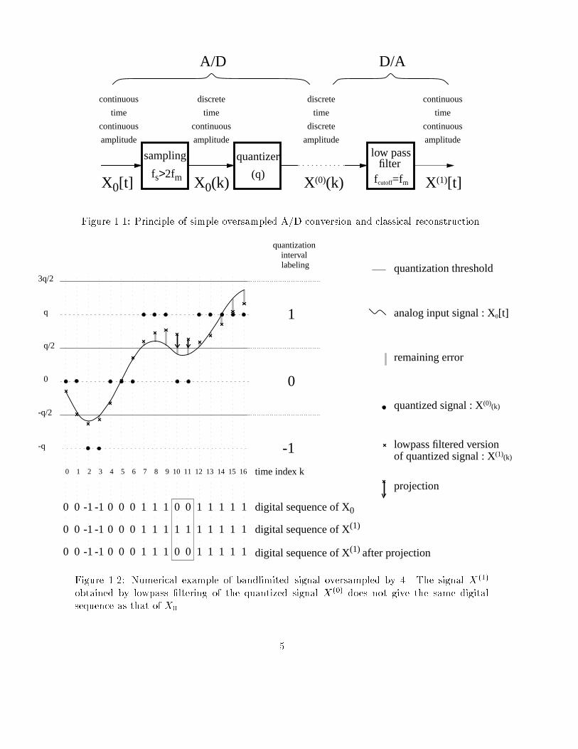
The motivation behind this criterion originally comes from the simple situation shownin �gure 1.2. We plot an example of bandlimited analog signal generated numerically andoversampled by 4. The crosses show the result of classical reconstruction in oversampledADC, obtained by lowpass �ltering the quantized signal (black dots). The �gure shows thatthis estimate does not yield the same digital sequence as the original. This can be seen attime indices 10 and 11. Let us now perform the following transformation: we project the twocritical samples of the estimate (k = 10 and k = 11) to the nearest border of the quantizationinterval which actually contains the original samples. This interval can be identi�ed from theknowledge of the original digital sequence. We end up with a new estimate which yields thesame digital sequence as that of the original analog signal and is at the same time better thanthe �rst estimate: the distance between the �rst estimate and the original signal has beennecessarily reduced. This improvement is automatic and does not depend on any assumptionabout the variations of the analog signal.Further remarks are appropriate to this simple example. Our estimate transformationdoes not require that quantization be uniform. It is based on the knowledge of the thresholds'position and is applicable whether the nonuniformity was designed or comes from circuit im-perfections. In the latter case we simply require the quantization thresholds of the converterto be measurable. As a second remark, we do not even require the thresholds to be constantin time, provided that their variations are known or can be determined. This is typically thesituation of dithered ADC. The particular condition here is that the dither be known in thetime domain. This is also the less obvious situation of �� and interpolative modulations,where, as will be shown in chapter 2, the feedback loop can be seen as a computable inputdither. Our last remark is the following: the reconstruction improvement of �gure 1.2 can bepushed further. Indeed, the new estimate has no reason to be bandlimited like the originalsignal. Therefore, it can be further improved with a second lowpass �ltering. Again, thesignal thus obtained may not yield the same digital output: the improvement procedure canbe reiterated.This simple example is in fact the starting point to our approach to ADC. What wasprecisely used in this example was the knowledge provided by the digital output of certainconstraints in amplitude that the input signal should meet. Qualitatively speaking, oncethese constraints are identi�ed, we can improve any estimate which does not meet them bya projection. If the digital sequence given by the input signal is C, these constraints can beexpressed as the set of all possible signals giving the same code sequence C. Conceptually,the description of an A/D converter can be reduced to a many-to-one mapping betweenanalog signals and digital sequences. The de�nition of the mapping only depends on theknowledge of the conversion's mechanisms (imperfections included). If this mapping can bedetermined, then the set of signals giving the same digital sequence C is the inverse image ofC through the mapping. We denote this set by �(C) and call it the signal cell of C. Sinceevery analog signal necessarily gives one and only one digital sequence, the inverse mappingassociated with the converter de�nes a partition of the space of input signals V (�gure 1.3).We call it the signal partition associated with the A/D converter.To identify estimates which have the same digital output as that of an original analogsignal, it is therefore essential to determine the signal partition de�ned by the A/D converter.In chapter 2, we show how to derive the mapping associated with a converter, and thus thesignal partition, on most A/D converters currently known: simple, dithered, predictive andnoise shaping ADC, including multi-stage modulators. We will observe that these convertersnaturally yield signal partitions where every cell is convex. This property justi�es the strongfact that, if an estimate X of an analog signal X0 giving the digital sequence C0 does not4

continuous

time

continuous

amplitude

continuous

time

continuous

amplitude

discrete

time

continuous

amplitude

discrete

time

discrete

amplitude

X0(k) fcutoff=fm

quantizersampling

X0[t] X(1)[t]fs>2fm (q)

low passfilter

A/D D/A

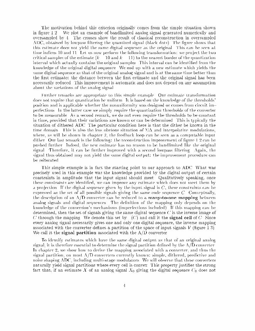
X(0)(k)Figure 1.1: Principle of simple oversampled A/D conversion and classical reconstruction.3q/2

q

q/2

0

-q/2

-q

0 1 2 3 4 5 6 7 8 9 10 11 12 13 14 15 16 time index k

quantizationinterval labeling

1

0

-1

0 0 -1-1 0 0 0 1 1 1 0 0 1 1 1 1

0 0 -1-1 0 0 0 1 1 1 1 1 1 1 1 1

0 0 -1-1 0 0 0 1 1 1 0 0 1 1 1 1

quantization threshold

analog input signal : X0[t]

remaining error

quantized signal : X(0)(k)

lowpass filtered versionof quantized signal : X(1)(k)

projection

1

1

1

digital sequence of X0

digital sequence of X(1)

digital sequence of X(1) after projectionFigure 1.2: Numerical example of bandlimited signal oversampled by 4. The signal X(1)obtained by lowpass �ltering of the quantized signal X(0) does not give the same digitalsequence as that of X0. 5

Γ(C5)

Γ(C6)

X0

Γ(C0)

Γ(C3)Γ(C4)

Γ(C2)

Γ(C1)

V

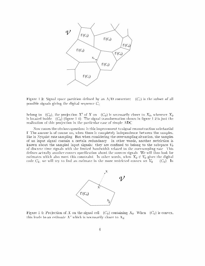
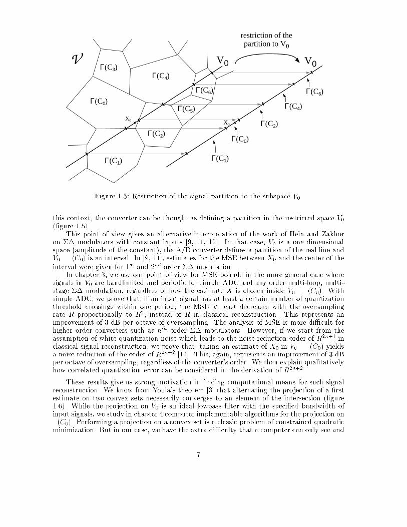
Figure 1.3: Signal space partition de�ned by an A/D converter: �(Ci) is the subset of allpossible signals giving the digital sequence Ci.belong to �(C0), the projection X 0 of X on �(C0) is necessarily closer to X0, wherever X0is located inside �(C0) (�gure 1.4). The signal transformation shown in �gure 1.2 is just therealization of this projection in the particular case of simple ADC.Now comes the obvious question: is this improvement to signal reconstruction substantial? The answer is of course no, when there is completely independence between the samples,like in Nyquist rate sampling. But when considering the oversampling situation, the samplesof an input signal contain a certain redundancy. In other words, another restriction isknown about the sampled input signals: they are con�ned to belong to the subspace V0of discrete time signals with the limited bandwidth related to the oversampling rate. Thisde�nes actually another convex speci�cation about the sources signals. We will thus look forestimates which also meet this constraint. In other words, when X0 2 V0 gives the digitalcode C0, we will try to �nd an estimate in the more restricted convex set V0 \ �(C0). InX0

Γ(C0)

X

X’

VFigure 1.4: Projection of X on the signal cell �(C0) containing X0. When �(C0) is convex,this leads to an estimate X 0 which is necessarily closer to X0.6

Γ(C5)

Γ(C6)

X0

Γ(C0)

V0

X0

Γ(C3)Γ(C4)

Γ(C2)

Γ(C1)

restriction of thepartition to V0

Γ(C1)

Γ(C2)

Γ(C4)

Γ(C6)

Γ(C0)

V V0

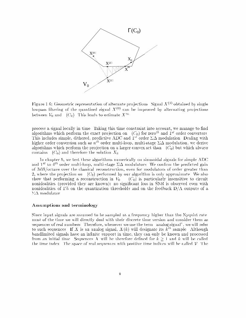
Figure 1.5: Restriction of the signal partition to the subspace V0.this context, the converter can be thought as de�ning a partition in the restricted space V0(�gure 1.5).This point of view gives an alternative interpretation of the work of Hein and Zakhoron �� modulators with constant inputs [9, 11, 12]. In that case, V0 is a one dimensionalspace (amplitude of the constant), the A/D converter de�nes a partition of the real line andV0 \�(C0) is an interval. In [9, 11], estimates for the MSE between X0 and the center of theinterval were given for 1st and 2nd order �� modulation.In chapter 3, we use our point of view for MSE bounds in the more general case wheresignals in V0 are bandlimited and periodic for simple ADC and any order multi-loop, multi-stage �� modulation, regardless of how the estimate X is chosen inside V0 \ �(C0). Withsimple ADC, we prove that, if an input signal has at least a certain number of quantizationthreshold crossings within one period, the MSE at least decreases with the oversamplingrate R proportionally to R2, instead of R in classical reconstruction. This represents animprovement of 3 dB per octave of oversampling. The analysis of MSE is more di�cult forhigher order converters such as nth order �� modulators. However, if we start from theassumption of white quantization noise which leads to the noise reduction order of R2n+1 inclassical signal reconstruction, we prove that, taking an estimate of X0 in V0 \ �(C0) yieldsa noise reduction of the order of R2n+2 [14]. This, again, represents an improvement of 3 dBper octave of oversampling, regardless of the converter's order. We then explain qualitativelyhow correlated quantization error can be considered in the derivation of R2n+2.These results give us strong motivation in �nding computational means for such signalreconstruction. We know from Youla's theorem [3] that alternating the projection of a �rstestimate on two convex sets necessarily converges to an element of the intersection (�gure1.6). While the projection on V0 is an ideal lowpass �lter with the speci�ed bandwidth ofinput signals, we study in chapter 4 computer implementable algorithms for the projection on�(C0). Performing a projection on a convex set is a classic problem of constrained quadraticminimization. But in our case, we have the extra di�culty that a computer can only see and7

X (0)

X0

X

X (1)

X (2)

Γ(C0)

V0

∞Figure 1.6: Geometric representation of alternate projections. Signal X(1) obtained by singlelowpass �ltering of the quantized signal X(0) can be improved by alternating projectionsbetween V0 and �(C0). This leads to estimate X1.process a signal locally in time. Taking this time constraint into account, we manage to �ndalgorithms which perform the exact projection on �(C0) for zeroth and 1st order converters.This includes simple, dithered, predictive ADC and 1st order �� modulation. Dealing withhigher order conversion such as nth order multi-loop, multi-stage �� modulation, we derivealgorithms which perform the projection on a larger convex set than �(C0) but which alwayscontains �(C0) and therefore the solution X0.In chapter 5, we test these algorithms numerically on sinusoidal signals for simple ADCand 1st to 4th order multi-loop, multi-stage �� modulators. We con�rm the predicted gainof 3dB/octave over the classical reconstruction, even for modulators of order greater than2, where the projection on �(C0) performed by our algorithm is only approximate. We alsoshow that performing a reconstruction in V0 \ �(C0) is particularly insensitive to circuitnonidealities (provided they are known): no signi�cant loss in SNR is observed even withnonidealities of 1% on the quantization thresholds and on the feedback D/A outputs of a�� modulator.Assumptions and terminologySince input signals are assumed to be sampled at a frequency higher than the Nyquist rate.most of the time we will directly deal with their discrete time version and consider them assequences of real numbers. Therefore, whenever we use the term \analog signal", we will referto such sequences. If X is an analog signal, X(k) will designate its kth sample. Althoughbandlimited signals have an in�nite support in time, they can only be known and processedfrom an initial time. Sequences X will be therefore de�ned for k � 1 and k will be calledthe time index. The space of real sequences with positive time indices will be called V . The8

canonical norm k � kV of V will be the mappingX 2 V 7�! kXkV = 0@Xk�1 jX(k)j21A1=2When considering periodic signals sampled on M points, it will be understood that V is thespace of M point sequences and kXkV = MXk=1 jX(k)j2!1=2A digital output C will be considered as a sequence of codewords C(k). We will often callit code sequence. We will use the term operator to denote a transformation which maps asequence into another sequence. The image sequence need not belong to the same space as theoriginal sequence. For example, an A/D converter is an operator which maps real sequencesinto code sequences. When an operator H maps X into Y , we will write Y = H [X ]. We willreserve the notation `DAC' for the operator of D/A conversion. For a given A/D converter,if a signal X0 gives a code sequence C0 the signal cell �(C0) will be also denoted by �(X0),depending on whether the object we are referring to is C0 or X0.

9

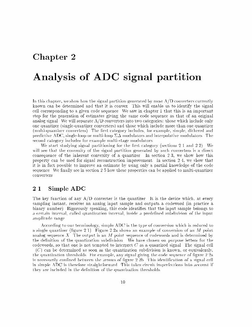
Chapter 2Analysis of ADC signal partitionIn this chapter, we show how the signal partition generated by most A/D converters currentlyknown can be determined and that it is convex. This will enable us to identify the signalcell corresponding to a given code sequence. We saw in chapter 1 that this is an importantstep for the generation of estimates giving the same code sequence as that of an originalanalog signal. We will separate A/D converters into two categories: those which include onlyone quantizer (single-quantizer converters) and those which include more than one quantizer(multi-quantizer converters). The �rst category includes, for example, simple, dithered andpredictive ADC, single-loop or multi-loop �� modulators and interpolative modulators. Thesecond category includes for example multi-stage modulators.We start studying signal partitioning for the �rst category (sections 2.1 and 2.2). Wewill see that the convexity of the signal partition generated by such converters is a directconsequence of the inherent convexity of a quantizer. In section 2.3, we show how thisproperty can be used for signal reconstruction improvement. In section 2.4, we show thatit is in fact possible to improve an estimate by using only a partial knowledge of the codesequence. We �nally see in section 2.5 how these properties can be applied to multi-quantizerconverters.2.1 Simple ADCThe key function of any A/D converter is the quantizer. It is the device which, at everysampling instant, receives an analog input sample and outputs a codeword (in practice abinary number). Rigorously speaking, this code identi�es that the input sample belongs toa certain interval, called quantization interval, inside a prede�ned subdivision of the inputamplitude range.According to our terminology, simple ADC is the type of conversion which is reduced toa single quantizer (�gure 2.1). Figure 2.2a shows an example of conversion of an M pointanalog sequence X . The output is an M point sequence of codewords and is determined bythe de�nition of the quantization subdivision. We have chosen on purpose letters for thecodewords, so that one is not tempted to interpret C as a quantized signal. The signal cell�(C) can be determined as soon as the quantization subdivision is known, or equivalently,the quantization thresholds. For example, any signal giving the code sequence of �gure 2.2ais necessarily con�ned between the arrows of �gure 2.2b. This identi�cation of a signal cellin simple ADC is therefore straightforward. This takes circuit imperfections into account ifthey are included in the de�nition of the quantization thresholds.10

CXquan- tizeranalog

sequencedigital

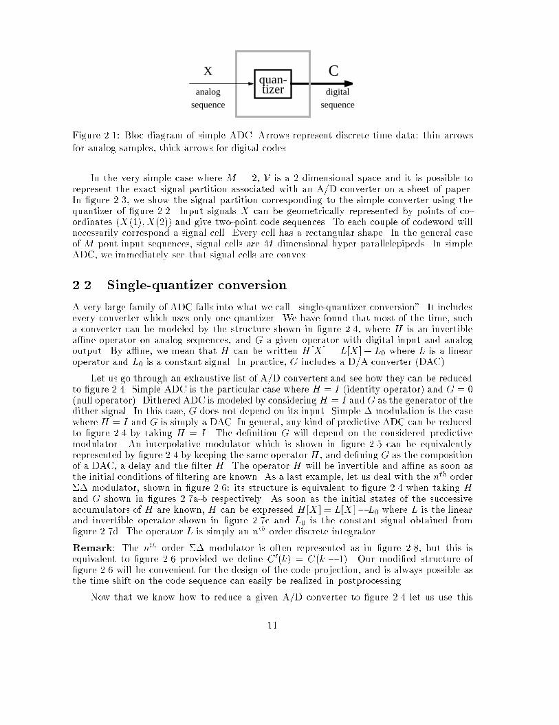
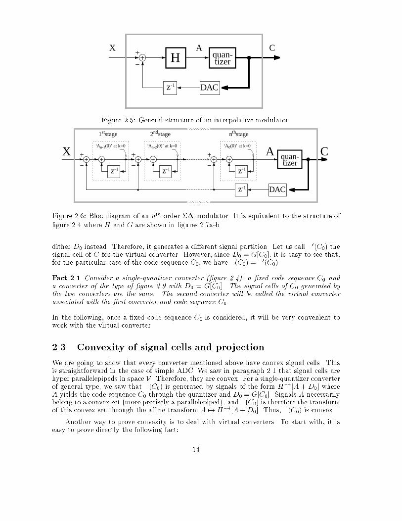
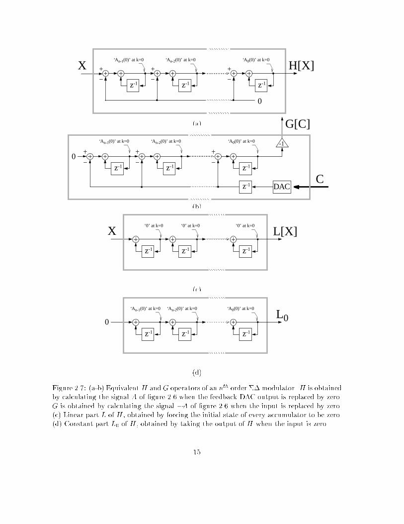
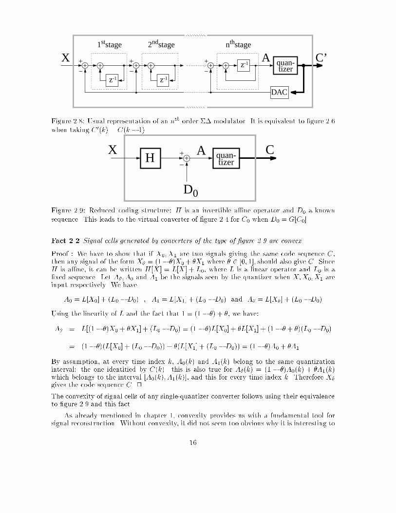
sequenceFigure 2.1: Bloc diagram of simple ADC. Arrows represent discrete time data: thin arrowsfor analog samples, thick arrows for digital codes.In the very simple case where M = 2, V is a 2 dimensional space and it is possible torepresent the exact signal partition associated with an A/D converter on a sheet of paper.In �gure 2.3, we show the signal partition corresponding to the simple converter using thequantizer of �gure 2.2. Input signals X can be geometrically represented by points of co-ordinates (X(1); X(2)) and give two-point code sequences. To each couple of codeword willnecessarily correspond a signal cell. Every cell has a rectangular shape. In the general caseof M pont input sequences, signal cells are M dimensional hyper parallelepipeds. In simpleADC, we immediately see that signal cells are convex.2.2 Single-quantizer conversionA very large family of ADC falls into what we call \single-quantizer conversion". It includesevery converter which uses only one quantizer. We have found that most of the time, sucha converter can be modeled by the structure shown in �gure 2.4, where H is an invertiblea�ne operator on analog sequences, and G a given operator with digital input and analogoutput. By a�ne, we mean that H can be written H [X ] = L[X ] + L0 where L is a linearoperator and L0 is a constant signal. In practice, G includes a D/A converter (DAC).Let us go through an exhaustive list of A/D converters and see how they can be reducedto �gure 2.4. Simple ADC is the particular case where H = I (identity operator) and G = 0(null operator). Dithered ADC is modeled by considering H = I and G as the generator of thedither signal. In this case, G does not depend on its input. Simple � modulation is the casewhere H = I and G is simply a DAC. In general, any kind of predictive ADC can be reducedto �gure 2.4 by taking H = I . The de�nition G will depend on the considered predictivemodulator. An interpolative modulator which is shown in �gure 2.5 can be equivalentlyrepresented by �gure 2.4 by keeping the same operator H , and de�ning G as the compositionof a DAC, a delay and the �lter H . The operator H will be invertible and a�ne as soon asthe initial conditions of �ltering are known. As a last example, let us deal with the nth order�� modulator, shown in �gure 2.6: its structure is equivalent to �gure 2.4 when taking Hand G shown in �gures 2.7a-b respectively. As soon as the initial states of the successiveaccumulators of H are known, H can be expressed H [X ] = L[X ]� L0 where L is the linearand invertible operator shown in �gure 2.7c and L0 is the constant signal obtained from�gure 2.7d. The operator L is simply an nth order discrete integrator.Remark: The nth order �� modulator is often represented as in �gure 2.8, but this isequivalent to �gure 2.6 provided we de�ne C 0(k) = C(k � 1). Our modi�ed structure of�gure 2.6 will be convenient for the design of the code projection, and is always possible asthe time shift on the code sequence can easily be realized in postprocessing.Now that we know how to reduce a given A/D converter to �gure 2.4 let us use this11

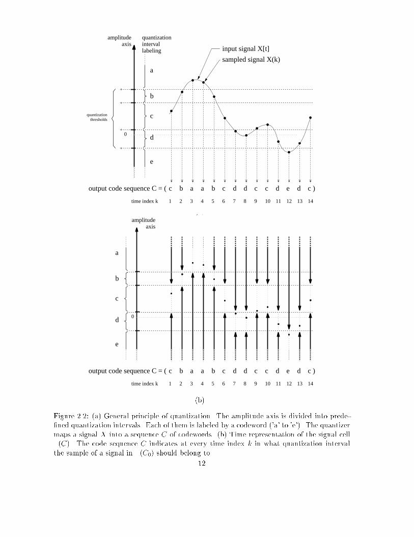
quantizationthresholds

amplitudeaxis

0

quantizationintervallabeling

a

b

c

d

e

aa bbc c c cd d d e d c )output code sequence C = (

input signal X[t]

sampled signal X(k)

1 2 3 4 5 6 7 8 9 10 11 12 13 14time index k (a)0

a

b

c

d

e

aa bbc c c cd d d e d c )output code sequence C = (

1 2 3 4 5 6 7 8 9 10 11 12 13 14time index k

amplitudeaxis

(b)Figure 2.2: (a) General principle of quantization. The amplitude axis is divided into prede-�ned quantization intervals. Each of them is labeled by a codeword ('a' to 'e'). The quantizermaps a signal X into a sequence C of codewords. (b) Time representation of the signal cell�(C). The code sequence C indicates at every time index k in what quantization intervalthe sample of a signal in �(C0) should belong to.12

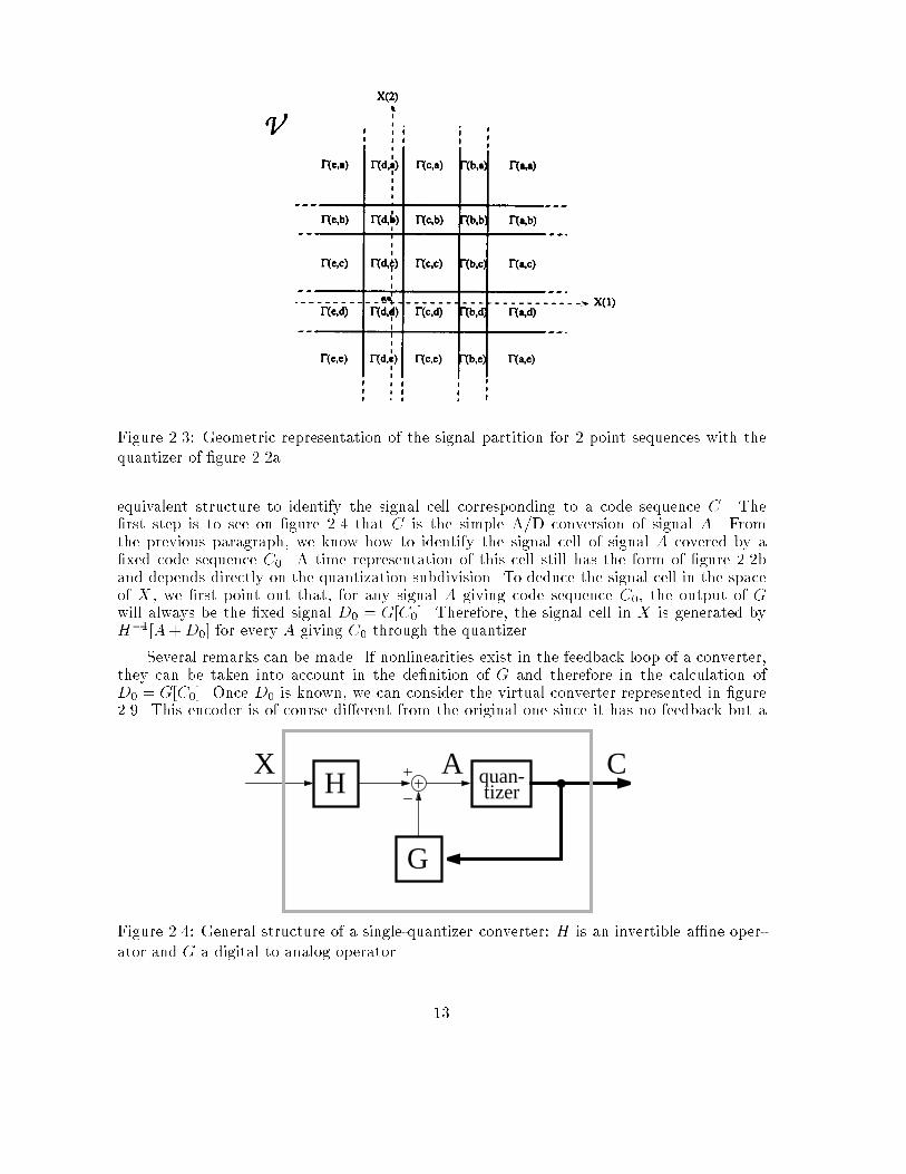
Figure 2.3: Geometric representation of the signal partition for 2 point sequences with thequantizer of �gure 2.2a.equivalent structure to identify the signal cell corresponding to a code sequence C. The�rst step is to see on �gure 2.4 that C is the simple A/D conversion of signal A. Fromthe previous paragraph, we know how to identify the signal cell of signal A covered by a�xed code sequence C0. A time representation of this cell still has the form of �gure 2.2band depends directly on the quantization subdivision. To deduce the signal cell in the spaceof X , we �rst point out that, for any signal A giving code sequence C0, the output of Gwill always be the �xed signal D0 = G[C0]. Therefore, the signal cell in X is generated byH�1[A+D0] for every A giving C0 through the quantizer.Several remarks can be made. If nonlinearities exist in the feedback loop of a converter,they can be taken into account in the de�nition of G and therefore in the calculation ofD0 = G[C0]. Once D0 is known, we can consider the virtual converter represented in �gure2.9. This encoder is of course di�erent from the original one since it has no feedback but aAX Cquan-

tizer

G

HFigure 2.4: General structure of a single-quantizer converter: H is an invertible a�ne oper-ator and G a digital to analog operator. 13

X

DAC

CAquan- tizerH

z-1Figure 2.5: General structure of an interpolative modulator.‘A 0(0)’ at k=0‘A n-1(0)’ at k=0 ‘A n-2(0)’ at k=0

DAC

1ststage 2ndstage nthstage

quan- tizer

z-1 z-1z-1

z-1

CX AFigure 2.6: Bloc diagram of an nth order �� modulator. It is equivalent to the structure of�gure 2.4 where H and G are shown in �gures 2.7a-b.dither D0 instead. Therefore, it generates a di�erent signal partition. Let us call �0(C0) thesignal cell of C for the virtual converter. However, since D0 = G[C0], it is easy to see that,for the particular case of the code sequence C0, we have �(C0) = �0(C0).Fact 2.1 Consider a single-quantizer converter (�gure 2.4), a �xed code sequence C0 anda converter of the type of �gure 2.9 with D0 = G[C0]. The signal cells of C0 generated bythe two converters are the same. The second converter will be called the virtual converterassociated with the �rst converter and code sequence C0.In the following, once a �xed code sequence C0 is considered, it will be very convenient towork with the virtual converter.2.3 Convexity of signal cells and projectionWe are going to show that every converter mentioned above have convex signal cells. Thisis straightforward in the case of simple ADC. We saw in paragraph 2.1 that signal cells arehyper parallelepipeds in space V . Therefore, they are convex. For a single-quantizer converterof general type, we saw that �(C0) is generated by signals of the form H�1[A + D0] whereA yields the code sequence C0 through the quantizer and D0 = G[C0]. Signals A necessarilybelong to a convex set (more precisely a parallelepiped), and �(C0) is therefore the transformof this convex set through the a�ne transform A 7! H�1[A+D0]. Thus, �(C0) is convex.Another way to prove convexity is to deal with virtual converters. To start with, it iseasy to prove directly the following fact: 14

0

z-1 z-1z-1

H[X]X‘A 0(0)’ at k=0‘A n-1(0)’ at k=0 ‘A n-2(0)’ at k=0(a)

DAC

G[C]

-1

0z-1 z-1z-1

z-1C

‘A 0(0)’ at k=0‘A n-1(0)’ at k=0 ‘A n-2(0)’ at k=0 (b)z-1 z-1z-1

L[X]X‘0’ at k=0‘0’ at k=0 ‘0’ at k=0(c)

L00

z-1 z-1z-1

‘A 0(0)’ at k=0‘A n-1(0)’ at k=0 ‘A n-2(0)’ at k=0(d)Figure 2.7: (a-b) Equivalent H and G operators of an nth order �� modulator. H is obtainedby calculating the signal A of �gure 2.6 when the feedback DAC output is replaced by zero.G is obtained by calculating the signal �A of �gure 2.6 when the input is replaced by zero.(c) Linear part L of H , obtained by forcing the initial state of every accumulator to be zero.(d) Constant part L0 of H , obtained by taking the output of H when the input is zero.15

C’1ststage 2ndstage nthstage

quan- tizer

z-1

z-1

z-1

DAC

X AFigure 2.8: Usual representation of an nth order �� modulator. It is equivalent to �gure 2.6when taking C 0(k) = C(k � 1).H quan-

tizer

D0

CX AFigure 2.9: Reduced coding structure: H is an invertible a�ne operator and D0 a knownsequence. This leads to the virtual converter of �gure 2.4 for C0 when D0 = G[C0].Fact 2.2 Signal cells generated by converters of the type of �gure 2.9 are convex.Proof : We have to show that if X0; X1 are two signals giving the same code sequence C,then any signal of the form X� = (1� �)X0+ �X1 where � 2 [0; 1], should also give C. SinceH is a�ne, it can be written H [X ] = L[X ] + L0, where L is a linear operator and L0 is a�xed sequence. Let A�; A0 and A1 be the signals seen by the quantizer when X;X0; X1 areinput respectively. We haveA0 = L[X0] + (L0 �D0) ; A1 = L[X1] + (L0 �D0) and A� = L[X�] + (L0 �D0)Using the linearity of L and the fact that 1 = (1� �) + �, we have:A� = L[(1� �)X0 + �X1] + (L0 �D0) = (1� �)L[X0] + �L[X1] + (1� � + �)(L0 �D0)= (1� �)(L[X0] + (L0 �D0)) + �(L[X1] + (L0 �D0)) = (1� �)A0 + �A1By assumption, at every time index k, A0(k) and A1(k) belong to the same quantizationinterval: the one identitied by C(k). this is also true for A�(k) = (1 � �)A0(k) + �A1(k)which belongs to the interval [A0(k); A1(k)], and this for every time index k. Therefore X�gives the code sequence C 2The convexity of signal cells of any single-quantizer converter follows using their equivalenceto �gure 2.9 and this fact.As already mentioned in chapter 1, convexity provides us with a fundamental tool forsignal reconstruction. Without convexity, it did not seem too obvious why it is interesting to16

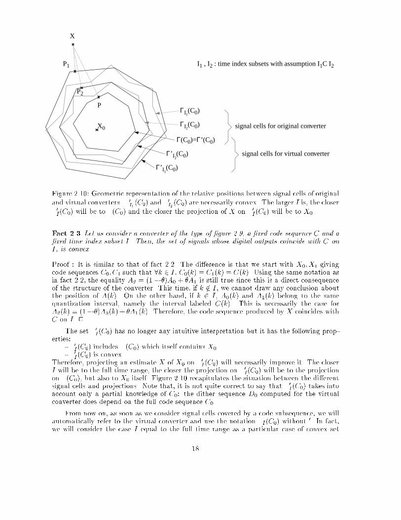
look for an estimate in �(C0). For example, this approach would seem inadequate if �(C0)was not connected (in one piece, roughly speaking). With convexity, we not only have theguarantee that �(C0) is connected, but we have a tool to (at least theoretically) improveany proposed estimate X which does not belong to the signal cell containing X0 namely theprojection on �(C0). By de�nition, the projection of X on �(C0) is the signal X 0 2 �(C0)which minimizes the distance with X . Because �(C0) is convex, it is a consequence of Hilbertspace properties that the distance between X 0 and X0 is necessarily inferior to that betweenX and X01.In chapter 4 we will actually propose algorithms to compute the projection of X on�(C0) in the case of simple, dithered, predictive ADC and the 1st order �� modulation.2.4 Signal cell of a code subsequence, convexity and projec-tionWhat really served us in the improvement of an estimate is the fact that �(C0) is a convexset that we can identify (because we know C0) and which contains X0 for sure. Actually, thisprinciple of estimate improvement will work as soon as we can identify a convex set whichcontains X0, whatever the method is, provided it is based on the available information. Inthis section, we prove that a partial knowledge of C0, more precisely, the knowledge of C0on a subset I of time indices, is enough to determine a convex set which necessarily containsX0. The search for such convex set will be very helpful in the future, especially when tryingto perform convex projections. Indeed, when the order of a converter becomes larger than 2,it will become unrealistic to compute the projection of an estimate, taking into account thesequence C0 on its full time range (chapter 4).The �rst attempt is to de�ne �I (C0) as the set of all signals giving code sequences whichcoincide with C0 only on the time subrange I :�I(C0) = fX 2 V / if X gives code C, 8k 2 I; C(k) = C0(k)gIt is obvious that �I(C0) contains �(C0) and therefore includes X0. More precisely, we havethe logic relation: if I1 � I2 then �I1(C0) � �I2(C0) � �(C0) 3 X0Qualitatively speaking, the closer I will be to the full time range, the closer �I(C0) will beto �(C0). Unfortunately, as suggested by our expression \�rst attempt", If I does not coverthe full time range, there is no reason for �I (C0) to be convex in general. The situation isnot hopeless.Once the code sequence C0 is �xed, we can always consider the associated virtual con-verter of �gure 2.9, which has the same signal cell �(C0). Let us call �0I(C0) the set of signalsgiving code sequences which coincide with C0 on I for the virtual converter. There is noreason to have �I (C0) = �0I(C0), but we will still have:if I1 � I2 then �0I1(C0) � �0I2(C0) � �0(C0) = �(C0) 3 X0Then we have the following fact:1To be rigorous, the projection X 0 exists (and is unique) only if �(C0) is also topologically closed. Actually,we will always consider the projection X 0 on �(C0), the closure of �(C0). Such a signal X 0 will not necessarilybelong to �(C0), but qualitatively speaking, will be at the limit to belong to it. Nevertheless, the propertywe e�ectively need is that X 0 is a better estimate of X0 than X.17

X

P1

P2

PΓI (C0)

Γ(C0)=Γ’(C0)

X0

1

Γ’ I (C0)2

Γ’ I (C0)1

ΓI (C0)2 signal cells for original converter

signal cells for virtual converter

I1 , I2 : time index subsets with assumption I1C I2

Figure 2.10: Geometric representation of the relative positions between signal cells of originaland virtual converters. �0I1(C0) and �0I2(C0) are necessarily convex. The larger I is, the closer�0I(C0) will be to �(C0) and the closer the projection of X on �0I (C0) will be to X0.Fact 2.3 Let us consider a converter of the type of �gure 2.9, a �xed code sequence C and a�xed time index subset I. Then, the set of signals whose digital outputs coincide with C onI, is convex.Proof : It is similar to that of fact 2.2. The di�erence is that we start with X0; X1 givingcode sequences C0; C1 such that 8k 2 I , C0(k) = C1(k) = C(k). Using the same notation asin fact 2.2, the equality A� = (1� �)A0 + �A1 is still true since this is a direct consequenceof the structure of the converter. This time, if k =2 I , we cannot draw any conclusion aboutthe position of A(k). On the other hand, if k 2 I , A0(k) and A1(k) belong to the samequantization interval, namely the interval labeled C(k). This is necessarily the case forA�(k) = (1� �)A0(k) + �A1(k). Therefore, the code sequence produced by X coincides withC on I 2The set �0I(C0) has no longer any intuitive interpretation but it has the following prop-erties:- �0I (C0) includes �(C0) which itself contains X0- �0I (C0) is convexTherefore, projecting an estimate X of X0 on �0I (C0) will necessarily improve it. The closerI will be to the full time range, the closer the projection on �0I(C0) will be to the projectionon �(C0), but also to X0 itself. Figure 2.10 recapitulates the situation between the di�erentsignal cells and projections. Note that, it is not quite correct to say that �0I(C0) takes intoaccount only a partial knowledge of C0: the dither sequence D0 computed for the virtualconverter does depend on the full code sequence C0.From now on, as soon as we consider signal cells covered by a code subsequence, we willautomatically refer to the virtual converter and use the notation �I (C0) without 0. In fact,we will consider the case I equal to the full time range as a particular case of convex set18

error

error

X single quantizerconverter 1

quantization

quantization

C1

C2

Cp

arith

met

ic s

tage

Csingle quantizer

converter 2

single quantizerconverter p(a)

error

error

X

quantization

quantization

C1

C2

Cp

C

single quantizerconverter 1

single quantizerconverter 2

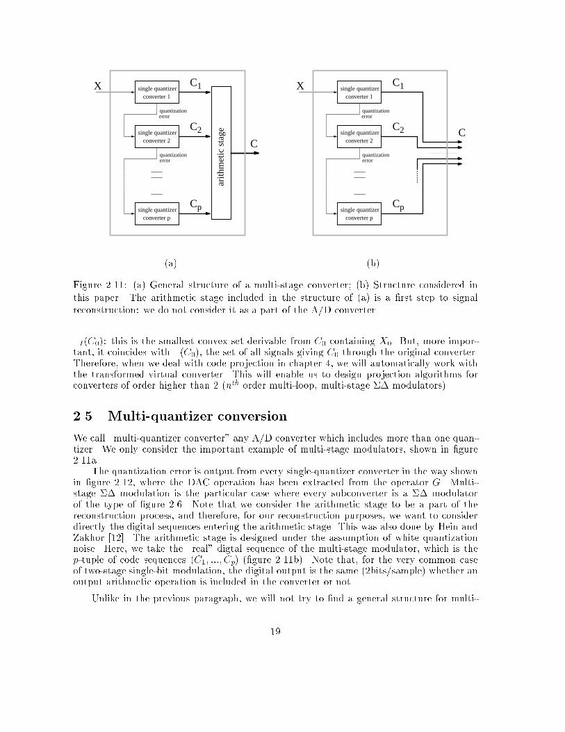
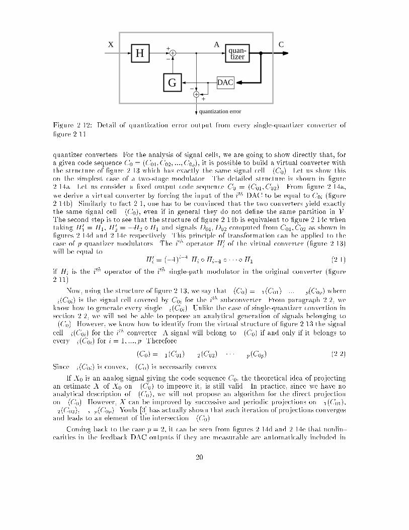
single quantizerconverter p(b)Figure 2.11: (a) General structure of a multi-stage converter; (b) Structure considered inthis paper. The arithmetic stage included in the structure of (a) is a �rst step to signalreconstruction: we do not consider it as a part of the A/D converter.�I(C0): this is the smallest convex set derivable from C0 containing X0. But, more impor-tant, it coincides with �(C0), the set of all signals giving C0 through the original converter.Therefore, when we deal with code projection in chapter 4, we will automatically work withthe transformed virtual converter. This will enable us to design projection algorithms forconverters of order higher than 2 (nth order multi-loop, multi-stage �� modulators)2.5 Multi-quantizer conversionWe call \multi-quantizer converter" any A/D converter which includes more than one quan-tizer. We only consider the important example of multi-stage modulators, shown in �gure2.11a.The quantization error is output from every single-quantizer converter in the way shownin �gure 2.12, where the DAC operation has been extracted from the operator G. Multi-stage �� modulation is the particular case where every subconverter is a �� modulatorof the type of �gure 2.6. Note that we consider the arithmetic stage to be a part of thereconstruction process, and therefore, for our reconstruction purposes, we want to considerdirectly the digital sequences entering the arithmetic stage. This was also done by Hein andZakhor [12]. The arithmetic stage is designed under the assumption of white quantizationnoise. Here, we take the \real" digtal sequence of the multi-stage modulator, which is thep-tuple of code sequences (C1; :::; Cp) (�gure 2.11b). Note that, for the very common caseof two-stage single-bit modulation, the digital output is the same (2bits/sample) whether anoutput arithmetic operation is included in the converter or not.Unlike in the previous paragraph, we will not try to �nd a general structure for multi-19

X

DAC

CAquan- tizer

G

H

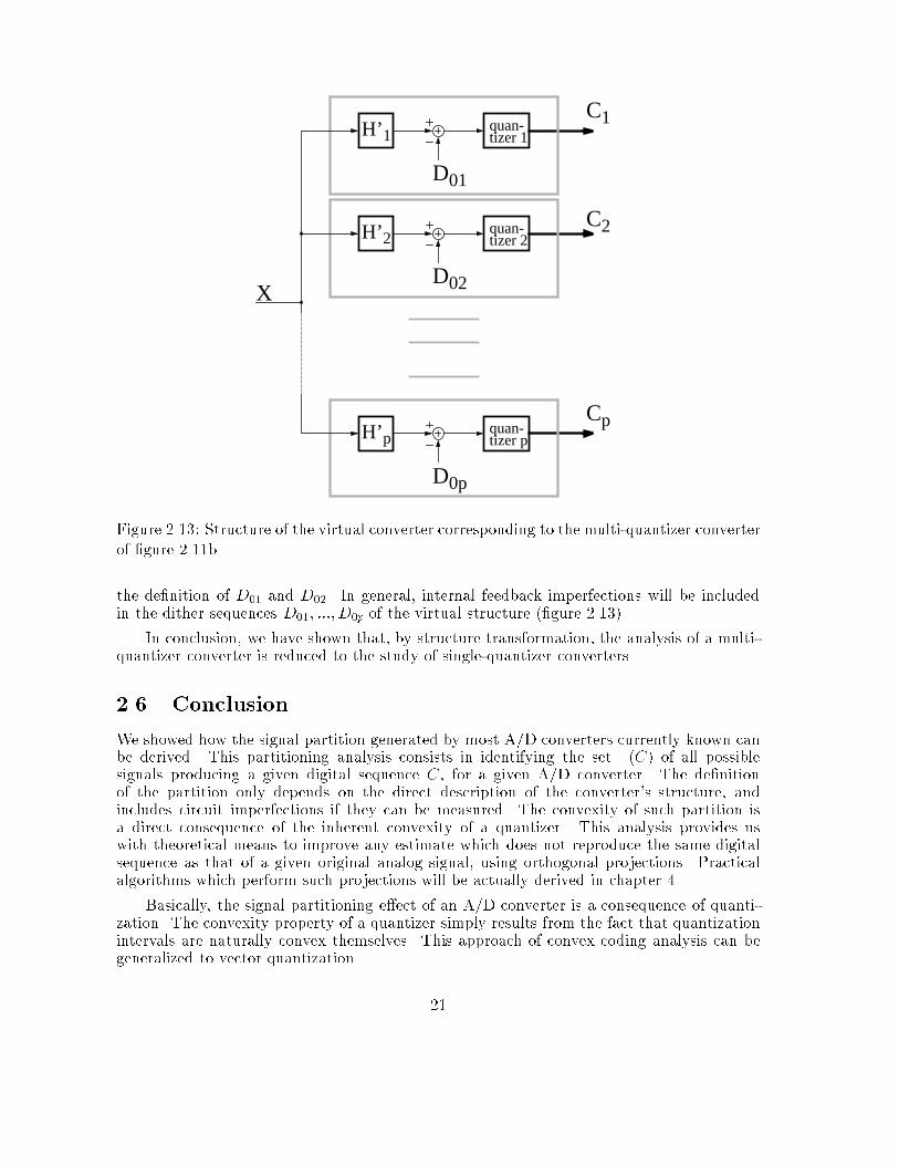
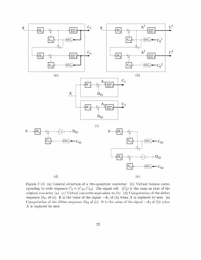
quantization errorFigure 2.12: Detail of quantization error output from every single-quantizer converter of�gure 2.11.quantizer converters. For the analysis of signal cells, we are going to show directly that, fora given code sequence C0 = (C01; C02; :::; C0p), it is possible to build a virtual converter withthe structure of �gure 2.13 which has exactly the same signal cell �(C0). Let us show thison the simplest case of a two-stage modulator. The detailed structure is shown in �gure2.14a. Let us consider a �xed output code sequence C0 = (C01; C02). From �gure 2.14a,we derive a virtual converter by forcing the input of the ith DAC to be equal to C0i (�gure2.14b). Similarly to fact 2.1, one has to be convinced that the two converters yield exactlythe same signal cell �(C0), even if in general they do not de�ne the same partition in V .The second step is to see that the structure of �gure 2.14b is equivalent to �gure 2.14c whentaking H 01 = H1, H 02 = �H2 �H1 and signals D01; D02 computed from C01; C02 as shown in�gures 2.14d and 2.14e respectively. This principle of transformation can be applied to thecase of p quantizer modulators. The ith operator H 0i of the virtual converter (�gure 2.13)will be equal to H 0i = (�1)i�1 Hi �Hi�1 � � � � �H1 (2.1)if Hi is the ith operator of the ith single-path modulator in the original converter (�gure2.11).Now, using the structure of �gure 2.13, we say that �(C0) = �1(C01)\ :::\�p(C0p) where�i(C0i) is the signal cell covered by C0i for the ith subconverter. From paragraph 2.2, weknow how to generate every single �i(C0i). Unlike the case of single-quantizer convertion insection 2.2, we will not be able to propose an analytical generation of signals belonging to�(C0). However, we know how to identify from the virtual structure of �gure 2.13 the signalcell �i(C0i) for the ith converter. A signal will belong to �(C0) if and only if it belongs toevery �i(C0i) for i = 1; :::; p. Therefore�(C0) = �1(C01) \ �2(C02)\ � � � \ �p(C0p) (2.2)Since �i(C0i) is convex, �(C0) is necessarily convex.If X0 is an analog signal giving the code sequence C0, the theoretical idea of projectingan estimate X of X0 on �(C0) to improve it, is still valid. In practice, since we have noanalytical description of �(C0), we will not propose an algorithm for the direct projectionon �(C0). However, X can be improved by successive and periodic projections on �1(C01),�2(C02), ...,�p(C0p). Youla [3] has actually shown that such iteration of projections convergesand leads to an element of the intersection �(C0).Coming back to the case p = 2, it can be seen from �gures 2.14d and 2.14e that nonlin-earities in the feedback DAC outputs if they are measurable are automatically included in20

H’2

H’1

H’p

C1

Cp

quan-tizer 1

D01

X

quan-tizer 2

D02

C2

quan-tizer p

D0pFigure 2.13: Structure of the virtual converter corresponding to the multi-quantizer converterof �gure 2.11b.the de�nition of D01 and D02. In general, internal feedback imperfections will be includedin the dither sequences D01; :::; D0p of the virtual structure (�gure 2.13).In conclusion, we have shown that, by structure transformation, the analysis of a multi-quantizer converter is reduced to the study of single-quantizer converters.2.6 ConclusionWe showed how the signal partition generated by most A/D converters currently known canbe derived. This partitioning analysis consists in identifying the set �(C) of all possiblesignals producing a given digital sequence C, for a given A/D converter. The de�nitionof the partition only depends on the direct description of the converter's structure, andincludes circuit imperfections if they can be measured. The convexity of such partition isa direct consequence of the inherent convexity of a quantizer. This analysis provides uswith theoretical means to improve any estimate which does not reproduce the same digitalsequence as that of a given original analog signal, using orthogonal projections. Practicalalgorithms which perform such projections will be actually derived in chapter 4.Basically, the signal partitioning e�ect of an A/D converter is a consequence of quanti-zation. The convexity property of a quantizer simply results from the fact that quantizationintervals are naturally convex themselves. This approach of convex coding analysis can begeneralized to vector quantization. 21

G1

G2

H2

H1

C1

C2

DAC2

DAC1

quan-tizer 1

quan-tizer 2

X

(a) C02

C01G1

G2

H2

H1quan-tizer 1

quan-tizer 2

X

DAC2

DAC1

C1

C2

A1

A2(b)H’2

H’1

A2

A1 quan-tizer 1

D01

quan-tizer 2

D02

C1

C2

X (c)G1

H1

C01

0

DAC1

-1 D01

(d) G1

G2

H2

H10

-1 D02

DAC2

DAC1

C02

C01(e)Figure 2.14: (a) General structure of a two-quantizer converter. (b) Virtual version corre-sponding to code sequence C0 = (C01; C02). The signal cell �(C0) is the same as that of theoriginal converter (a). (c) Virtual converter equivalent to (b). (d) Computation of the dithersequence D01 of (c). It is the value of the signal �A1 of (b) when X is replaced by zero. (e)Computation of the dither sequence D02 of (c). It is the value of the signal �A2 of (b) whenX is replaced by zero. 22

Chapter 3MSE analysis of optimal signalreconstruction in oversampledADCIn this chapter, we suppose that input signals belong to the subspace V0 � V of sequencesbandlimited to a known maximum frequency fm: this is the situation of oversampled ADC.Once a signal X0 2 V0 is given by a code sequence C0 output by a given A/D converter,we propose to study the estimation of X0 which consists in \picking up" a signal insideV0 \ �(C0). Theoretically, it is possible to reach such a signal by alternating projections of a�rst estimate on V0 and �(C0) (Youla's theorem [3]). As said in chapter 1, we will proposealgorithms which actually perform these projections, in chapter 4.We study MSE bounds of such estimates, �rst for the simple ADC and then for anysingle-quantizer converter where the operator H is a cascade of integrators (�gure 2.4). Thisincludes, for example, the nth order multi-loop �� modulator. As a consequence, we will seethat MSE bounds can be deduced for multi-stage, multi-loop �� modulators as well. Heinand Zakhor measured MSE upper bounds for the 1st and 2nd order �� modulators in theparticular case of dc input (one dimensional V0) [9, 11].In our MSE bound evaluation, we will not make any assumption about how the estimateX ofX0 is chosen inside V0\�(C0). Thus our analysis will be applicable to any reconstructionmethod leading to a reconstructed signal inside V0 \ �(C0).3.1 Modelization of bandlimited and periodic signals (V0)Continuous time bandlimited periodic signals of period T0 can be expressed as follows:X [t] = A+ NXj=1Bjp2 cos(2�j tT0 ) + NXj=1Cjp2 sin(2�j tT0 ) (3.1)Such signals have 2N + 1 discrete low frequency components, between �NT0 and NT0 in thecontinuous Fourier domain. They can be equivalently described by their sampled version:X(k) = X h kMT0i = A+ NXj=1Bjp2 cos(2�j kM ) + NXj=1Cjp2 sin(2�j kM ) (3.2)23

when choosing the sampling frequency of the form MT0 such that M > 2N + 1 (oversamplingsituation). In this section, we will consider that V0 is the space of sequences of the form(3.2) for a �xed N , with the assumption that M > 2N + 1. Note that the oversamplingrate R is proportional to M . An element of V0 given by (3.2) (or (3.1)) is uniquely de�nedby the vector ~X 2 R2N+1 whose components are (A;B1; :::; BN ; C1; :::; CN). In other words,we have an isomorphism between V0 and R2N+1. The dimension of V0 is therefore 2N + 1.Using Parseval's equality, it can be derived that1M MXk=1 jX(k)j2 = A2 + NXj=1B2j + NXj=1C2j = k ~Xk2where jj ~Xjj is the canonical norm in R2N+1. Therefore, if X 2 V0 \ �(X0) is an estimate ofX0 2 V0, the mean squared error MSE(X0; X) between X0 and X can be measured by thedistance in R2N+1 between their associated vectors ~X0 and ~X:MSE(X0; X) = 1M MXk=1 jX(k)�X0(k)j2 = k ~X � ~X0k2 (3.3)We will use this isometry between V0 and R2N+1 throughout this section. We will in particu-lar try to measure the asymptotic evolution of this MSE bound with increasing oversamplingrate. Since M is proportional to R, we will compare the MSE with powers of M .3.2 Simple ADCWe recall that for simple ADC, the classical signal reconstruction yields a gain in SNR of3dB per octave of oversampling. Increasing R by an octave means doubling the resolutionin time of the signal discretization. It is interesting to see that when the resolution inamplitude is doubled, the gain is not 3dB but 6dB (in short, the gain is 6dB per bit). Intheory, one would like to think ADC as a homogeneous discretization of a two dimensionalgraph, where the dimensions are amplitude and time. One could argue that the origin of thisdi�erence is the non-homogeneity of the error measurement: the MSE is a measure of errorsonly along the amplitude dimension. However, a bandlimited signal has a bounded slope.Therefore, qualitatively speaking, variations in the time dimension should be observable inthe amplitude dimension with a bounded multiplicative coe�cient which should not a�ectthe logarithmic dependence of the MSE. These considerations give another hint that theclassical signal reconstruction in simple ADC is not optimal.In the theorem we are about to present, we show that, in the context of periodic signals,an estimate X of X0 chosen in V0 \ �(X0) will yield an MSE which goes to zero at leastas fast as �M2 when M goes to +1, where � is a constant independent of M : this actuallyrepresents a gain of 6dB per octave of oversampling. This property is however veri�ed undera certain condition about the source signal X0: it must cross the quantization thresholds atleast 2N + 1 times. This condition relative to the amplitude dimension is in fact the dualcondition to the restriction in the time dimension that M should be larger than 2N + 1. Ifthe last condition fails, aliasing will result from sampling and introduce an irreversible erroreven before the signal is quantized in amplitude. Obviously, the 6dB/bit gain should not beexpected in this case. Similarly, if the number of threshold crossings is less than 2N + 1, thegain of 6dB per octave of oversampling should not be expected either.24

Theorem 3.1 If the continuous time version of a signal X0 2 V0 has more than 2N + 1quantization threshold crossings1, there exists a constant c0 which only depends on X0 suchthat, for M large enough and any X in V0 \ �(X0), MSE(X0; X)� c0M2Proof : The set of instants where X0[t] is equal to one of the threshold levels is discreteand �nite (since X0 cannot be constant). Let �t0 > 0 be the minimum distance betweenthese instants. We consider M large enough (or Ts = T0M small enough) so that Ts < �t03 .Let us choose 2N +1 distinct threshold crossings of X0[t], call (t00; :::; t02N) their instants and(l1; :::; l2N) their levels.We are �rst going to show that any signal X 2 V0 \ �(X0) necessarily crosses levelli at an instant ti in the same sampling interval as that of t0i , for every i = 0; :::; 2N . Let(k0; :::; k2N) be the time indices such that the sampling interval Ii = [(ki�1)Ts; kiTs] containst0i for every i = 0; :::; 2N . For a �xed i, X0[t] crosses level li which is the common boundaryof two quantization intervals. Because Ts < �t0, X0(ki � 1) and X0(ki) necessarily belongrespectively to the interior of these two intervals. If X 2 V0 \ �(X0), X(ki � 1) and X(ki)should respectively belong to the quantization intervals which contain X0(ki�1) and X0(ki).Therefore, since it is continuous, X [t] should cross level li at a time ti 2 Ii. As a consequence,we have jti � t0i j � Ts = T0M (3.4)Since Ts < �t03 , we also have8i1; i2 2 f0; :::; 2Ng such that i1 6= i2; jti1 � ti2 j > �t03 (3.5)Using (3.4), we are going to show to that the norm of ~X � ~X0 can be linearly bounded with1M when M goes to +1. This will be based on a linearization of variations in time and analgebraic manipulation.Using (3.1), the fact that X [ti] = X0[t0i ] = li for every i = 0; :::; 2N can be written witha vector notation as M(t0; :::; t2N) ~X =M(t00; :::; t02N) ~X0 = ~L (3.6)where M(s0; :::; s2N) is the transpose of the square matrix26666666666664 1 � � � 1p2 cos(2�s0=T0) � � � p2 cos(2�s2N=T0)... � � � ...p2 cos(2�Ns0=T0) � � � p2 cos(2�Ns2N=T0)p2 sin(2�s0=T0) � � � p2 sin(2�s2N=T0)... � � � ...p2 sin(2�Ns0=T0) � � � p2 sin(2�Ns2N=T0) 377777777777751We will not count as threshold crossings, points where X0[t] reaches a threshold without crossing it. Asa consequence, X0 cannot be a constant 25

and ~L the column vector whose components are (l0; :::; l2N). Replacing the cos and sin func-tions inM by their complex exponential expressions, it is possible to see thatM(s0; :::; s2N)is similar to the Vandermonde matrix[exp(j2�ksi=T0)]0�i�2N;�N�k�Nwhich is invertible as soon as (s0; :::; s2N) are distinct. Therefore,M(t0; :::; t2N) andM(t00; :::; t02N)are invertible. It can also be shown that, because of (3.5), �M(t00; :::; t02N)��1 is bounded.Therefore, ~X = �M(t00; :::; t02N)��1 ~L is bounded. SubtractingM(t00; :::; t02N) ~X in the two �rstmembers of equation (3.6), we �ndM(t00; :::; t02N)( ~X � ~X0) = � �M(t0; :::; t2N)�M(t00; :::; t02N)� ~X (3.7)At the limit of M going to +1, ti � t0i goes to zero and we haveM(t0; :::; t2N)�M(t00; :::; t02N) ' 2NXi=0(ti � t0i )@M@ti (t00; :::; t02N) (3.8)Because ~X is bounded and M(t00; :::; t02N) is invertible, (3.7) and (3.8) imply that~X � ~X0 ' � hM(t00; :::; t02N)i�1 2NXi=0(ti � t0i )@M@ti (t00; :::; t02N) ~X (3.9)Since ~X is bounded, the right hand side goes to zero when M goes to +1. Therefore, ~Xtends to ~X0, and (3.9) is still true when replacing ~X by ~X0 in the right hand side (since~X0 6= ~0). We obtain ~X � ~X0 ' 2NXi=0(ti � t0i ) ~F 0iwhere ~F 0i = � hM(t00; :::; t02N)i�1 @M@ti (t00; :::; t02N) ~X0is a vector which depends only on the signal X0. Using (3.4), we �nd jj ~X � ~X0jj � cM wherec = T0P2Ni=0 jj ~F 0i jj. The proof is completed using (3.3) and taking c0 = c2 2Remark : The only assumption used in this theorem was the number of threshold crossingsof the input signal. For example, this does not require quantization to be uniform. However,the constant c0 obtained in the upper bound may depend on how the input signal crossesthe thresholds. In particular, c0 depends on ~F 0i which contains the term @M@ti (t00; :::; t02N) ~X0.One can verify that this expression contains the slope of X0 at the ith threshold crossing.3.3 nth order single-quantizer converterIn theorem 3.1, we needed the condition that the source signal has at least 2N +1 thresholdcrossings within its period. We saw that this is the amplitude dimension dual condition to26

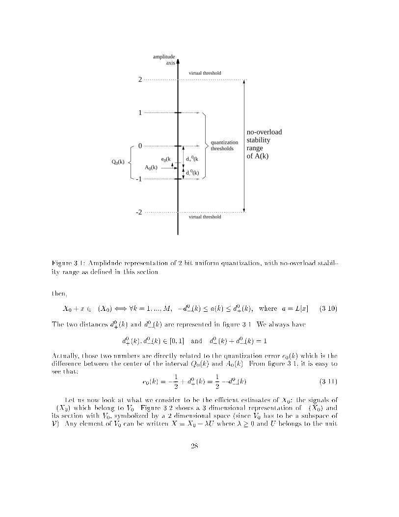
the time dimension condition which requires that M > 2N + 1. Indeed, M represents thenumber of \sampling time crossings" of the signal. Since signals are function of time, there isa trivial equality between the number of sampling instants and the number of sampling timecrossings. Unfortunately, this is not the case in the amplitude dimension. In general, withrigid quantization thresholds, there is no way to control the number of threshold crossingsof a signal, unless particular characteristics are known from it. Then, it becomes naturalto think of time varying quantization thresholds. The idea is that, in simple ADC, thee�cient information is located around the threshold crossings of the input signal, whereasthe rest of the time is just \waiting". Making the quantization thresholds vary in time isincreasing the chances to \intercept" the signal. This is what happens in single-quantizerconverters of �gure 2.4 when the output of G is not a constant signal. Indeed, if we forgetthe presence of the operator H for a moment, the code sequence gives the comparison ofsignal Y with the quantization thresholds shifted by the time varying output of G. Thislast signal can be prede�ned (dithered ADC) or calculated from the digital output (generalcase of a single-quantizer converter). In order to evaluate the MSE between X0 and anestimate X 2 V0 \ �(C0), we cannot think in terms of threshold crossings any more: sincethe variations of the G output can be abrupt, we have lost the notion of bounded slope andcannot use di�erentiation tools. We have to study how the G output directly a�ects thede�nition of V0 \ �(C0).To reduce the di�culty of the problem, we are going to con�ne ourselves to only considerconverters where H is an nth order integrator, and the quantizer is uniform with a step sizeequal to 1 and a �nite number of intervals. We naturally include the single-bit quantizer.Moreover, we suppose that the analog signals X to be coded verify a no-overload stabilitycondition that we de�ne as follows: the signal A seen by the quantizer when X is input,never goes farther than a distance equal to 1 from the extreme quantization thresholds.For example, in the case of �rst order �� modulation, any signal X where every samplebelongs to [�12 ; 12 ], will automatically verify the stability condition when the output valuesof the feedback DAC are �12 . In this context, we will assume that an estimate X0 of X inV0 \ �(X0) should also verify this stability condition. We can include this constraint in thede�nition of �(X0) by considering that the two extreme quantization intervals, which arenormally of in�nite length, have a size equal to 1 (see �gure 3.1). We will then automaticallyreject as estimate of X0, any signal which gives the same code as X0 but does not verifythe stability condition. Finally, in our characterization of V0 \ �(X0) for a given X0, itwill be convenient to consider the virtual converter. This is always possible, since the setof signals giving the same code as X0 is the same whether we look at the original or thevirtual converter (fact 2.1). The interesting feature about the virtual converter is the simplecharacterization of the signal seen by the quantizer. Indeed, when X is input, the signal Aappearing in front of the quantizer is A = H [X ]� G[C0] whether X belongs to �(X0) ornot. Since we want to study the distance or the di�erence between X and X0, it will beconvenient to rewrite this last relation as A�A0 = L[X �X0], where L is the linear part ofH . If we express X = X0 + x, then A = A0 + a where a = L[x].Let us �rst try to characterize the elements of �(X0). The action of the G feedbackis re ected in the behavior of signal A0 = H [X0] � G[C0]. But, to recognize that a signalX belongs to �(X0), what really matters is only the relative position of A0(k) within thequantization interval Q0(k) it belongs to. Indeed, X = X0 + x will belong to �(X0) if andonly if, at every instant k, A0(k) + a(k) and A0(k) belong to the same quantization interval.If we call d0+(k) and d0�(k) the distance of A0(k) to the upper and lower bounds of Q0(k)27

2

e0(k

no-overloadstabilityrangeof A(k)

quantizationthresholds

d+0(k

d-0(k)

1

0

-1

-2

virtual threshold

virtual threshold

amplitudeaxis

A0(k)Q0(k)

Figure 3.1: Amplidude representation of 2 bit uniform quantization, with no-overload stabil-ity range as de�ned in this section.then,X0 + x 2 �(X0)() 8k = 1; :::;M; �d0�(k) � a(k) � d0+(k); where a = L[x] (3.10)The two distances d0+(k) and d0�(k) are represented in �gure 3.1. We always haved0+(k); d0�(k) 2 [0; 1] and d0+(k) + d0�(k) = 1Actually, those two numbers are directly related to the quantization error e0(k) which is thedi�erence between the center of the interval Q0(k) and A0(k). From �gure 3.1, it is easy tosee that: e0(k) = �12 + d0+(k) = 12 � d0�(k) (3.11)Let us now look at what we consider to be the e�cient estimates of X0: the signals of�(X0) which belong to V0. Figure 3.2 shows a 3 dimensional representation of �(X0) andits section with V0, symbolized by a 2 dimensional space (since V0 has to be a subspace ofV). Any element of V0 can be written X = X0 + �U where � � 0 and U belongs to the unit28

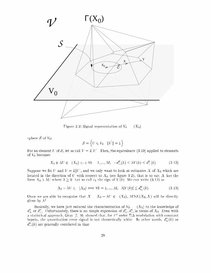
Γ(X0)

XY

UX0

V0

S

V

Figure 3.2: Signal representation of V0 \ �(X0).sphere S of V0: S = nU 2 V0.k~Uk = 1oFor an element U of S, let us call V = L[U ]. Then, the equivalence (3.10) applied to elementsof V0 becomesX0 + �U 2 �(X0)() 8k = 1; :::;M; �d0�(k) � �V (k) � d0+(k) (3.12)Suppose we �x U and V = L[U ], and we only want to look at estimates X of X0 which arelocated in the direction of ~U with respect to X0 (see �gure 3.2), that is to say, X has theform X0 + �U where � � 0. Let us call �k the sign of V (k). We can write (3.12) asX0 + �U 2 �(X0)() 8k = 1; :::;M; �jV (k)j � d0�k(k) (3.13)Once we are able to recognize that X = X0 + �U 2 �(X0), MSE(X0; X) will be directlygiven by �2.Basically, we have just reduced the characterization of V0 \ �(X0) to the knowledge ofd0+ or d0�. Unfortunately, there is no simple expression of d0+; d0� in terms of X0. Even witha statistical approach, Gray [7, 10] showed that, for 1st order �� modulation with constantinputs, the quantization error signal is not theoretically white. In other words, d0+(k) ord0�(k) are generally correlated in time. 29

However, without the knowledge of d0+ or d0�, the mere fact that A0(k) is con�ned in aninterval of size 1 already gives a �rst upper bound to MSE(X0; X) where X 2 V0 \ �(X0).From (3.13), an estimate X0 + �U in �(X0) at least veri�es�jV (k)j � 1; 8k = 1; :::;M (3.14)We recall that V is the result of the nth order integration of U . To give an intuition of theupper bound, let us look at the particular direction ~U where U is the unit constant signal:8k = 1; :::;M; U(k) = 1. In this case, without calculation, we will expect V (k) to growwith k in a fashion comparable to knn! . Therefore, V (k) will reach its maximum at k = M .From (3.14), we necessarily have � � 1V (M) ' n!Mn . We conclude that, if X 2 V0 \ �(X0)di�ers from X0 by a constant signal, we necessarily have MSE(X0; X) � cM2n where c > 0is a constant independent of M .We are going to show that this dependence of the MSE with respect to M is the samewith every other direction U of S. This time the maximum of jV (k)j is not necessarilyachieved at k =M , but we still have from (3.14) the necessary condition� � 1max1�k�M jV (k)j (3.15)The following lemma shows that, even if U is not the constant signal, but is in general aperiodic and bandlimited signal of energy 1, then max1�k�M jV (k)j is still proportional toMn.Lemma 3.2 When L is the nth order integrator, there exist two constants 0 < c1 < c2 suchthat, for M large enough,8U 2 S; c1Mn � max1�k�M jV (k)j � c2Mn; where V = L[U ]This is proved in appendix A.1. As a natural consequence, we haveFact 3.3 There exists a constant c > 0 such that, for M large enough, for any input X0 2 V0which satis�es the stability condition,8X 2 V0 \ �(X0); MSE(X0; X) � cM2nProof : Use the necessary condition (3.15), the lower bound of lemma 3.2, use the fact thatMSE(X0; X) = �2 and take c = 1c212Of course, this upper bound is not satisfactory, since the classical reconstruction itselfhas a 1M2n+1 behavior. In particular, when n = 0 such as in dithered or predictive ADC, fact3.3 does not show any expectation of MSE improvement with increasing oversampling ratio.The weakness of this upper bound comes from the fact that, in the application of (3.13), wedid not do better than assuming that d0�k(k) = 1, 8k; U . Even if d0�k(k) is strongly correlatedin time, we would expect d0�k(k) to be sometimes less than 1. Think that, in (3.13), it isthe smallest d0�k(k) for k = 1; :::;M which will impose the strongest constraint on �. In fact,this is not entirely true because jV (k)j also varies with k. But, still, this idea gives us a�rst hint to a deeper analysis. Let us see what happens if we assume that for any sequence30

of signs (�1; :::; �M), (d0�1(1); :::; d0�M(M)) are independent random variables with a uniformdistribution in [0; 1]. This is completely equivalent to saying that the quantization errorsignal e0 is white with a uniform distribution in [�12 ; 12 ]. We know this is not theoreticallytrue, but this approach will still give us some insight. As a �rst curiosity, we would like toknow what would be the expected value of the minimum of (d0�1(1); :::; d0�M(M)) in terms ofthe number M of considered random variables. We have the following result:Fact 3.4 Let (d(1); :::; d(M)) beM independent random variables with a uniform distributionin [0; 1], and dmin = min1�k�m d(k). Then dmin is a random variable and its expected valueis 1M+1Proof : Prob(dmin � �) = Prob(8k = 1; :::;M; d(k) � �) = (1� �)MProb(dmin 2 [�; �+ d�]) = � dd�(Prob(dmin � �))d� =M(1� �)M�1d�E(dmin) = R 10 �M(1� �)M�1d� = 1M+1 2If by chance the maximum of jV (k)j and the minimum of d0�k (k) are achieved at the sametime, then (3.13) will imply � � 1max1�k�M jV (k)j min1�k�M d0�k(k)which qualitatively reduces the upper bound of � by a factor of 1M , and the upper bound of�2 by 1M2 . Of course this is not likely to happen, but we will see that some compromise willbe found.One has to think of jV (k)j as a slowly varying function, and this for two reasons: V is theresult of an nth order integration of some signal U , which itself is a slowly varying function,especially for high oversampling ratios. We just want to give the intuition that the behaviorjV (k)j � c1Mn is true at a substantial number of time indices other than when jV (k)jachieves its maximum. Actually, it will appear in our derivation that the upper bound ofthe MSE expectation is more precisely related to the average of jV (k)j. The following lemmasays that the average of jV (k)j has the same behavior as its maximum value, with respect toM .Lemma 3.5 When L is the nth order integrator, there exist two constants 0 < c3 < c4 suchthat, for M large enough,8U 2 S; c3Mn � 1M MXk=1 jV (k)j � c4Mn; where V = L[U ]This is proved in appendix A.1. As a consequence, we have the following fact:Theorem 3.6 Suppose that when the input signal X0 is taken at random in the stabilityrange of V0, for any M � 1, the quantization error values (e0(1); :::; e0(M)) are independentrandom variables with a uniform distribution in [0; 1]. Then there exists a constant c > 0such that, for M large enough, E(MSE(X0; X)) � cM2n+2where X is taken at random in V0 \ �(X0). 31

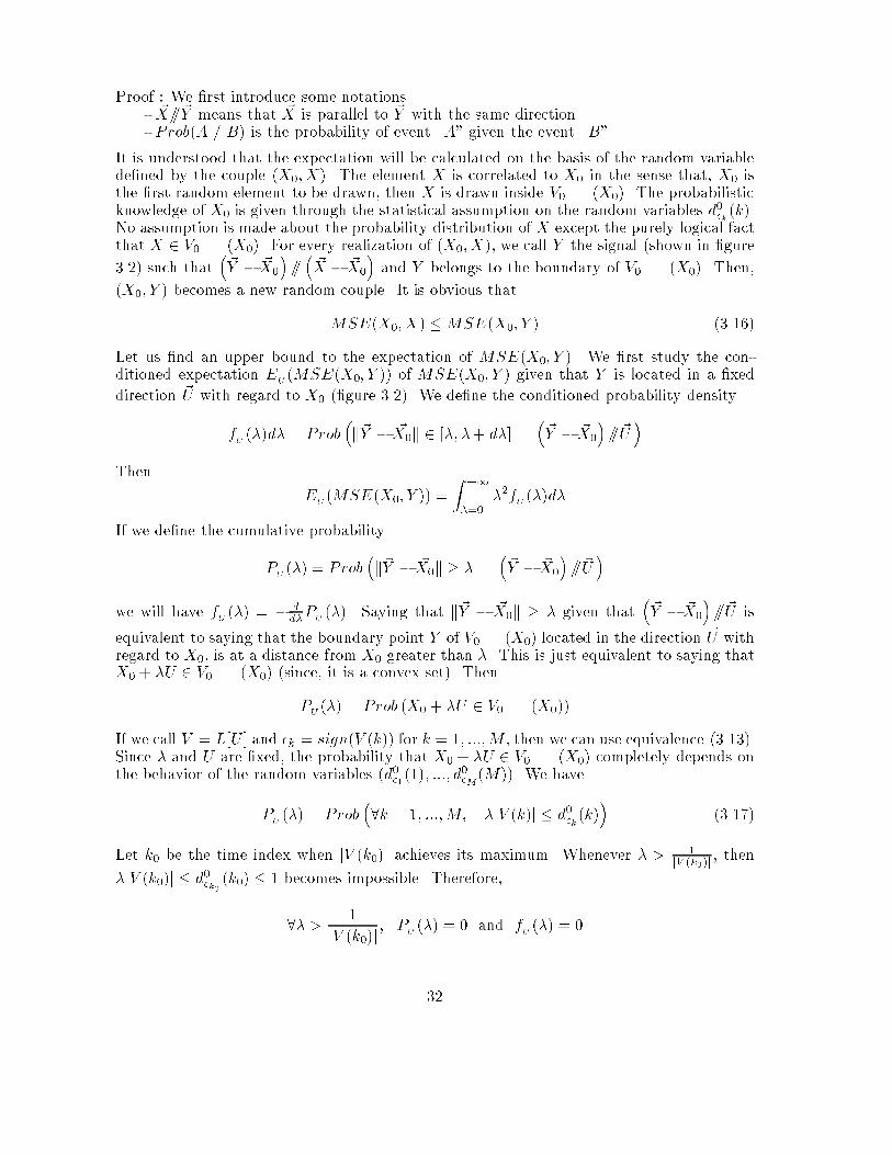
Proof : We �rst introduce some notations.- ~X==~Y means that ~X is parallel to ~Y with the same direction.- Prob(A = B) is the probability of event \A" given the event \B".It is understood that the expectation will be calculated on the basis of the random variablede�ned by the couple (X0; X). The element X is correlated to X0 in the sense that, X0 isthe �rst random element to be drawn, then X is drawn inside V0 \ �(X0). The probabilisticknowledge of X0 is given through the statistical assumption on the random variables d0�k(k).No assumption is made about the probability distribution of X except the purely logical factthat X 2 V0 \ �(X0). For every realization of (X0; X), we call Y the signal (shown in �gure3.2) such that �~Y � ~X0� == � ~X � ~X0� and Y belongs to the boundary of V0 \ �(X0). Then,(X0; Y ) becomes a new random couple. It is obvious thatMSE(X0; X) �MSE(X0; Y ) (3.16)Let us �nd an upper bound to the expectation of MSE(X0; Y ). We �rst study the con-ditioned expectation EU (MSE(X0; Y )) of MSE(X0; Y ) given that Y is located in a �xeddirection ~U with regard to X0 (�gure 3.2). We de�ne the conditioned probability densityfU (�)d� = Prob �k~Y � ~X0k 2 [�; �+ d�] . �~Y � ~X0� ==~U �Then EU (MSE(X0; Y )) = Z +1�=0 �2fU (�)d�If we de�ne the cumulative probabilityPU (�) = Prob �k~Y � ~X0k � � . �~Y � ~X0� ==~U �we will have fU (�) = � dd�PU (�). Saying that k~Y � ~X0k � � given that �~Y � ~X0� ==~U isequivalent to saying that the boundary point Y of V0\�(X0) located in the direction ~U withregard to X0, is at a distance from X0 greater than �. This is just equivalent to saying thatX0 + �U 2 V0 \ �(X0) (since, it is a convex set). ThenPU (�) = Prob (X0 + �U 2 V0 \ �(X0))If we call V = L[U ] and �k = sign(V (k)) for k = 1; :::;M , then we can use equivalence (3.13).Since � and U are �xed, the probability that X0 + �U 2 V0 \ �(X0) completely depends onthe behavior of the random variables (d0�1(1); :::; d0�M(M)). We havePU (�) = Prob �8k = 1; :::;M; �jV (k)j � d0�k(k)� (3.17)Let k0 be the time index when jV (k0)j achieves its maximum. Whenever � > 1jV (k0)j , then�jV (k0)j � d0�k0 (k0) � 1 becomes impossible. Therefore,8� > 1jV (k0)j ; PU (�) = 0 and fU (�) = 032

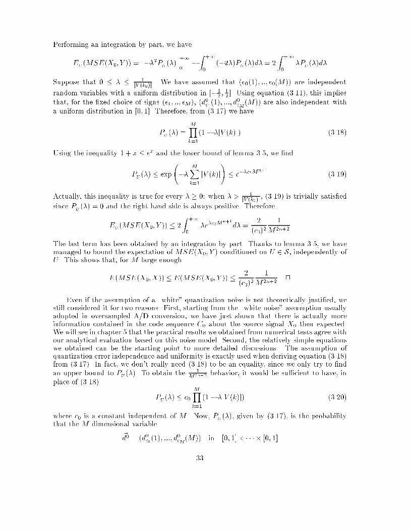
Performing an integration by part, we haveEU (MSE(X0; Y )) = h��2PU (�)i+10 � Z +10 (�2�)PU (�)d�= 2 Z +10 �PU (�)d�Suppose that 0 � � � 1jV (k0)j . We have assumed that (e0(1); ::; e0(M)) are independentrandom variables with a uniform distribution in [�12 ; 12 ]. Using equation (3.11), this impliesthat, for the �xed choice of signs (�1; ::; �M), (d0�1(1); :::; d0�M(M)) are also independent witha uniform distribution in [0; 1]. Therefore, from (3.17) we havePU (�) = MYk=1(1� �jV (k)j) (3.18)Using the inequality 1 + x � ex and the lower bound of lemma 3.5, we �ndPU (�) � exp �� MXk=1 jV (k)j! � e��c3Mn+1 (3.19)Actually, this inequality is true for every � � 0: when � > 1jV (k0)j , (3.19) is trivially satis�edsince PU (�) = 0 and the right hand side is always positive. ThereforeEU (MSE(X0; Y )) � 2 Z +10 �e�c3Mn+1d� = 2(c3)2 1M2n+2The last term has been obtained by an integration by part. Thanks to lemma 3.5, we havemanaged to bound the expectation of MSE(X0; Y ) conditioned on U 2 S, independently ofU . This shows that, for M large enoughE(MSE(X0; X))� E(MSE(X0; Y )) � 2(c3)2 1M2n+2 2Even if the assumption of a \white" quantization noise is not theoretically justi�ed, westill considered it for two reasons. First, starting from the \white noise" assumption usuallyadopted in oversampled A/D conversion, we have just shown that there is actually moreinformation contained in the code sequence C0 about the source signal X0 then expected.We will see in chapter 5 that the practical results we obtained from numerical tests agree withour analytical evaluation based on this noise model. Second, the relatively simple equationswe obtained can be the starting point to more detailed discussions. The assumption ofquantization error independence and uniformity is exactly used when deriving equation (3.18)from (3.17). In fact, we don't really need (3.18) to be an equality, since we only try to �ndan upper bound to PU (�). To obtain the 1M2n+2 behavior, it would be su�cient to have, inplace of (3.18) PU (�) � c0 MYk=1(1� �jV (k)j) (3.20)where c0 is a constant independent of M . Now, PU (�), given by (3.17), is the probabilitythat the M dimensional variable~d0 = (d0�1(1); :::; d0�M(M)) in [0; 1]� � � � � [0; 1]33

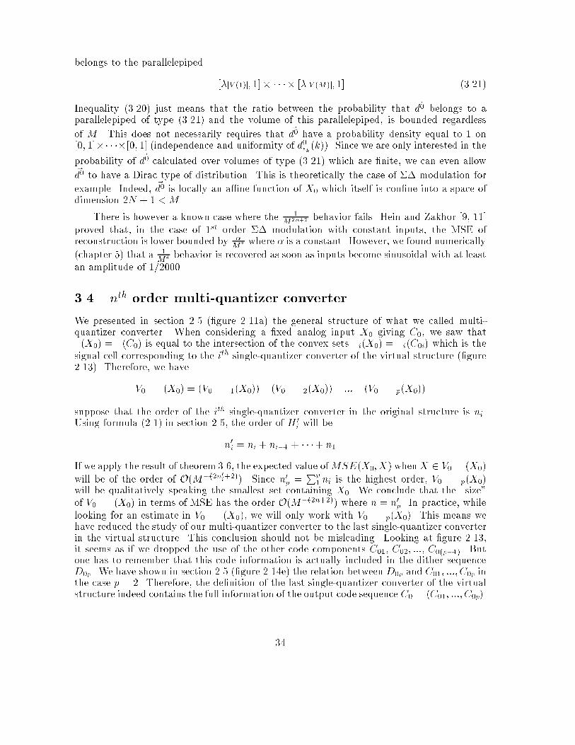
belongs to the parallelepiped [�jV (1)j; 1]� � � � � [�jV (M)j; 1] (3.21)Inequality (3.20) just means that the ratio between the probability that ~d0 belongs to aparallelepiped of type (3.21) and the volume of this parallelepiped, is bounded regardlessof M . This does not necessarily requires that ~d0 have a probability density equal to 1 on[0; 1]�� � �� [0; 1] (independence and uniformity of d0�k(k)). Since we are only interested in theprobability of ~d0 calculated over volumes of type (3.21) which are �nite, we can even allow~d0 to have a Dirac type of distribution. This is theoretically the case of �� modulation forexample. Indeed, ~d0 is locally an a�ne function of X0 which itself is con�ne into a space ofdimension 2N + 1 < M .There is however a known case where the 1M2n+2 behavior fails. Hein and Zakhor [9, 11]proved that, in the case of 1st order �� modulation with constant inputs, the MSE ofreconstruction is lower bounded by �M3 where � is a constant. However, we found numerically(chapter 5) that a 1M4 behavior is recovered as soon as inputs become sinusoidal with at leastan amplitude of 1=2000.3.4 nth order multi-quantizer converterWe presented in section 2.5 (�gure 2.11a) the general structure of what we called multi-quantizer converter. When considering a �xed analog input X0 giving C0, we saw that�(X0) = �(C0) is equal to the intersection of the convex sets �i(X0) = �i(C0i) which is thesignal cell corresponding to the ith single-quantizer converter of the virtual structure (�gure2.13). Therefore, we haveV0 \ �(X0) = (V0 \ �1(X0))\ (V0 \ �2(X0)) \ :::\ (V0 \ �p(X0))suppose that the order of the ith single-quantizer converter in the original structure is ni.Using formula (2.1) in section 2.5, the order of H 0i will ben0i = ni + ni�1 + � � �+ n1If we apply the result of theorem 3.6, the expected value ofMSE(X0; X) whenX 2 V0\�(X0)will be of the order of O(M�(2n0i+2)). Since n0p = Pp1 ni is the highest order, V0 \ �p(X0)will be qualitatively speaking the smallest set containing X0. We conclude that the \size"of V0 \ �(X0) in terms of MSE has the order O(M�(2n+2)) where n = n0p. In practice, whilelooking for an estimate in V0 \ �(X0), we will only work with V0 \ �p(X0). This means wehave reduced the study of our multi-quantizer converter to the last single-quantizer converterin the virtual structure. This conclusion should not be misleading. Looking at �gure 2.13,it seems as if we dropped the use of the other code components C01, C02; :::, C0(p�1). Butone has to remember that this code information is actually included in the dither sequenceD0p. We have shown in section 2.5 (�gure 2.14e) the relation between D0p and C01; :::; C0p inthe case p = 2. Therefore, the de�nition of the last single-quantizer converter of the virtualstructure indeed contains the full information of the output code sequence C0 = (C01; :::; C0p).34

3.5 ConclusionWorking on periodic input signals, we have shown under certain assumptions that picking anestimate X of an original signals X0, having the same bandwidth and producing the samedigital sequence, leads to an MSE upper bounded by R�(2n+2) instead of R�(2n+1), where Ris the oversampling rate and n is the order of the converter. For simple ADC (n = 0), thisis conditioned on the fact that the original signal X0 has a minimum number of thresholdcrossings. For single-quantizer converters of higher order (n � 1), the MSE has a necessaryupper bound proportional to R�(2n+2) when assuming no-overload stability and a white anduniform quantization error signal. We explained, however, that this result can be obtainedwith weaker assumptions. This analysis can be applied to a multi-quantizer converter since itcan be decomposed into single-quantizer converters working in parallel, according to chapter2. As a consequence, the overall performance is still R�(2n+2) where n is the total order ofthe multi-quantizer converter.

35

Chapter 4Algorithms for the projection on�I(C0)4.1 IntroductionIn this chapter, we propose computer implementable algorithms to perform the projection ofa signal X on �I(C0) for a given single-quantizer converter, a code sequence C0 and a timeindex subset I . The set �I(C0) is de�ned in section 2.4 and is systematically derived fromthe virtual converter. When I is the whole time range, then �I(C0) coincides with �(C0),the set of all analog signals giving code sequence C0 through the original converter. We sawthat �I(C0) is always convex. Even if our study is based on the general case where I is notnecessarily the full time range, whenever we can, we will try to �nd a method to perform theprojection on �(C0), since �(C0) gives the best localization of X0 based on the knowledge ofC0. Otherwise, we will try to �nd the projection on �I(C0) where I is as large as possible,or, in other words, �I(C0) is as close as possible to �(C0). Our particular motivation willbe to test the performance of the proposed algorithm in the context of oversampled ADC(chapter 5), and compare the results with the analysis of chapter 3.From section 2.3 we know that the projection of X on �I (C0) is the signal X 0 2 �I (C0)which minimizes the mean squared error with respect to X . We immediatly recognize theproblem on a constrained minimization: X 0 minimizes the function Y 7! MSE(X; Y ) sub-ject to the constraint Y 2 �I(C0). We can then apply the theory of optimization in thecontext of quadratic minimization function with convex constraints. However, we have totake into account the fact that elements we want to optimize are signals de�ned on a wholetime interval. It is of course expected that a computer can only process a signal througha moving �nite length window (typically, the length of the bu�er). Conceptually, the totallength of signals should be thought of as in�nite compared to that of the window of opera-tion. Therefore, we have to design speci�c optimization algorithms, adapted to this practicalconstraint. We will see in section 4.3 that, in the case of zeroth order conversion (simple,dithered or predictive ADC), the minimization of MSE(X;X 0) subject to X 0 2 �I(C0) canbe performed by an independent computation of X 0(k) at time k, only function of X(k) andD0(k) at the same instant (D0 is the dither sequence derived from the virtual converter of�gure 2.9). This will enable us to propose a straightforward algorithm for the projectionon �(C0). Unfortunately, this is no longer true with converters of higher order. For 1storder �� modulation (section 4.4) we will see that X 0(k) has to be computed by blocks intime. However, the computation is independent from one block to another. We propose an36

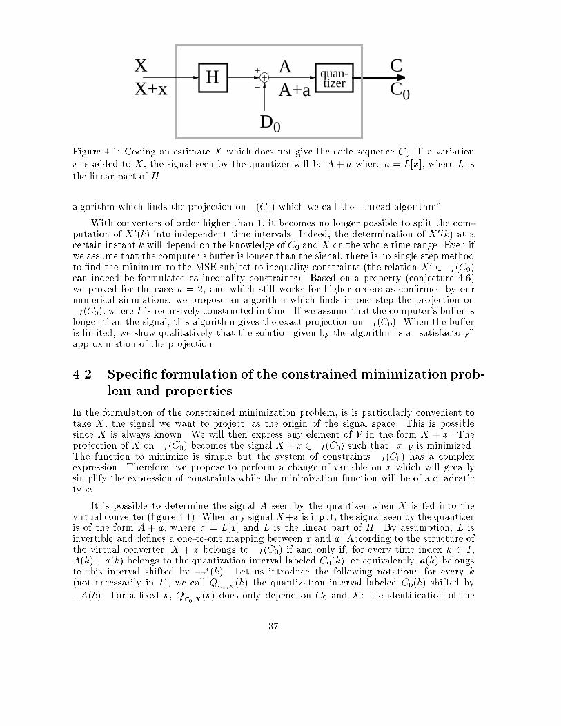
H quan- tizer

D0

CX AC0X+x A+aFigure 4.1: Coding an estimate X which does not give the code sequence C0. If a variationx is added to X , the signal seen by the quantizer will be A + a where a = L[x], where L isthe linear part of H .algorithm which �nds the projection on �(C0) which we call the \thread algorithm".With converters of order higher than 1, it becomes no longer possible to split the com-putation of X 0(k) into independent time intervals. Indeed, the determination of X 0(k) at acertain instant k will depend on the knowledge of C0 and X on the whole time range. Even ifwe assume that the computer's bu�er is longer than the signal, there is no single step methodto �nd the minimum to the MSE subject to inequality constraints (the relation X 0 2 �I (C0)can indeed be formulated as inequality constraints). Based on a property (conjecture 4.6)we proved for the case n = 2, and which still works for higher orders as con�rmed by ournumerical simulations, we propose an algorithm which �nds in one step the projection on�I(C0), where I is recursively constructed in time. If we assume that the computer's bu�er islonger than the signal, this algorithm gives the exact projection on �I(C0). When the bu�eris limited, we show qualitatively that the solution given by the algorithm is a \satisfactory"approximation of the projection.4.2 Speci�c formulation of the constrained minimization prob-lem and propertiesIn the formulation of the constrained minimization problem, is is particularly convenient totake X , the signal we want to project, as the origin of the signal space. This is possiblesince X is always known. We will then express any element of V in the form X + x. Theprojection of X on �I (C0) becomes the signal X + x 2 �I(C0) such that kxkV is minimized.The function to minimize is simple but the system of constraints �I(C0) has a complexexpression. Therefore, we propose to perform a change of variable on x which will greatlysimplify the expression of constraints while the minimization function will be of a quadratictype.It is possible to determine the signal A seen by the quantizer when X is fed into thevirtual converter (�gure 4.1). When any signal X+x is input, the signal seen by the quantizeris of the form A + a, where a = L[x] and L is the linear part of H . By assumption, L isinvertible and de�nes a one-to-one mapping between x and a. According to the structure ofthe virtual converter, X + x belongs to �I (C0) if and only if, for every time index k 2 I ,A(k) + a(k) belongs to the quantization interval labeled C0(k), or equivalently, a(k) belongsto this interval shifted by �A(k). Let us introduce the following notation: for every k(not necessarily in I), we call QC0;X (k) the quantization interval labeled C0(k) shifted by�A(k). For a �xed k, QC0 ;X (k) does only depend on C0 and X : the identi�cation of the37

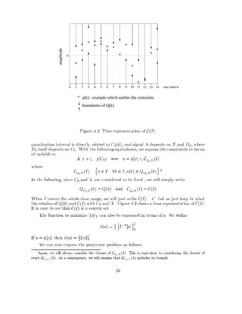
time index k0 654321 7 8 9 10 12 1311

0

ampl

itude

a(k) : example which satifies the contraints

14

boundaries of Q(k)Figure 4.2: Time representation of C(I).quantization interval is directly related to C0(k), and signal A depends on X and D0, whereD0 itself depends on C0. With the following equivalence, we express the constraints in termsof variable a: X + x 2 �I (C0) () a = L[x] 2 CC0;X (I)where CC0;X (I) = na 2 V .8k 2 I; a(k) 2 QC0;X (k)o 1In the following, since C0 and X are considered to be �xed , we will simply writeQC0;X (k) = Q(k) and CC0 ;X (I) = C(I)When I covers the whole time range, we will just write C(I) = C. Let us just keep in mindthe relation of Q(k) and C(I) with C0 and X . Figure 4.2 shows a time representation of C(I).It is easy to see that C(I) is a convex set.The function to minimize kxkV can also be expressed in terms of a. We de�ne�(a) = 12 L�1[a] 2VIf a = L[x], then �(a) = 12kxk2V .We can now express the projection problem as follows:1Again, we will always consider the closure of CC0;X (I). This is equivalent to considering the closure ofevery QC0 ;X (k). As a consequence, we will assume that QC0;X (k) includes its bounds.38

Fact 4.1 The projection of X on �I(C0) is the signal X + x such that x = L�1[a] and a isthe minimum of � subject to the constraint C(I) = fa 2 V /8k 2 I; a(k) 2 Q(k)gSince � is a quadratic function and C(I) a convex set, the theory of optimization directlycon�rms that � has a unique minimum subject to C(I). This theory also provides a charac-terization of the minimum when � is quadratic, which is the case here. If we designate by@�@a the sequence whose value @�@a (k) at time k is the partial derivative of �(a) with respect toa(k), we have the following theorem:Theorem 4.2 (Euler inequality characterization) A signal a0 is a minimum of � sub-ject to convex constraints S if and only ifa0 2 S and 8a 2 S; Xk @�@a0 (k) � (a(k)� a0(k)) � 0 (4.1)Thanks to the change of variable x$ a, the constraint speci�cation C(I) has the particularadvantage to be separable. By this we mean that constraints are de�ned independentlyof a(k) at every time index k. As a consequence of Euler characterization, the theory ofoptimization provides us with the following theorem:Theorem 4.3 Let a0 be a minimum of � subject to separable convex constraints S. Then8k; 8a 2 S; @�@a0 (k) � (a(k)� a0(k)) � 0 (4.2)If for a certain index k, S does not impose any constraint on a(k), then@�@a0 (k) = 0 (4.3)Proof : Let us consider a �xed time index k1, and a �xed element a1 2 S. Let a01 be thesequence equal to a0 everywhere except at instant k = k1 where a01(k1) = a1(k1). Since a0 2 Sand S is separable, a01 also belongs to S. Applying (4.1) on a = a1, we �nd @�@a0 (k1)(a1(k1)�a0(k1)) � 0. This proves (4.2). To show (4.3), suppose that at k = k1, S does not impose anyconstraint on a(k1). Let a+; a� be the sequences equal to a0 everywhere except at k = k1where a+(k1) = a0(k1) + 1 and a�(k1) = a0(k1) � 1. We have a+; a� 2 S. Then applying(4.1) on a = a+ and a = a�, we respectively �nd @�@a0 (k1) � 0 and � @�@a0 (k1) � 0, whichimplies that @�@a0 (k1) = 0 2If the change of variable x$ a simpli�es the constraints expression, it however compli-cates the function to minimize �. In this chapter, we will only consider converters where Lis an nth order integrator. In this case, using notation 4.4, @�@a can be obtained according tofact 4.5.Notation 4.4 nth order discrete derivativeFor y 2 V, y(n)� and y(n)+ are the nth order discrete backward and forward derivatives of yrecursively de�ned as follows: y(0)� = y(0)+ = y39

and for n � 0 ( y(n+1)�(1) = y(n)�(1)y(n+1)�(k) = y(n)�(k)� y(n)�(k� 1) ; for k � 1and y(n+1)+(k) = y(n)+(k + 1)� y(n)+(k) ; for k � 0Fact 4.5 If L is an nth order integrator (�gure 2.7) and a = L[x], thenx = a(n)� and @�@a = (�1)nx(n)+This is shown in appendix A.2.4.3 Zeroth order converter (simple, dithered, predictive ADC)This is the easy case where H = L = identity. We will immediately consider the projectionon �(C0). We will derive an algorithm directly without using any of the theorems of theprevious section.Signal A is just X � D0 where D0 is the zero signal in simple ADC, the dither signalin dithered ADC and the feedback output in predictive ADC. Variables x and a are thusidentical and the function to minimize is �(a) = 12kak2V which is proportional to Pk ja(k)j2.Since the constraint C(I) is a system of conditions applied to samples a(k) taken separately,the minimization of Pk ja(k)j2 is equivalent to the individual minimization of each ja(k)j. Ifk 2 I , a0(k) is necessarily the element of Q(k) of lowest magnitude. Figure 4.3 shows anexample of minimization solution. This leads to the following algorithm:Algorithm 1 : Given the knowledge of C0 and X , at every time index k:(1) - calculate D0(k) the value of the feedback signal G[C0] at time k(2) - calculate A(k) = X(k)�D0(k)(3) - determine Q(k), the quantization interval labeled C0(k) shifted by �A(k)(4) - if Q(k) contains 0, take a0(k) = 0otherwise, take a0(k) equal to the closest bound of Q(k) to 0.Then, X + a0, where a0 results from this algorithm, is the projection of X on �I(C0).In the particular case of simple ADC (D0 = 0), one can check that this leads to thetransformation we introduced in chapter 1 (�gure 1.2).4.4 1st order converter (1st order �� modulation)In this case L is a single discrete integrator (n = 1). According to fact 4.5, if L[x] = a, thenx(k) = a(k)� a(k � 1) is the slope of a at time k and@�@a = �fx(k + 1)� x(k)g = �f(a(k+ 1)� a(k))� (a(k)� a(k � 1))gis minus the change of slope of a about time index k. Here again, we consider that I coversthe whole time range. We propose an algorithm that we describe in a \physical" way.40

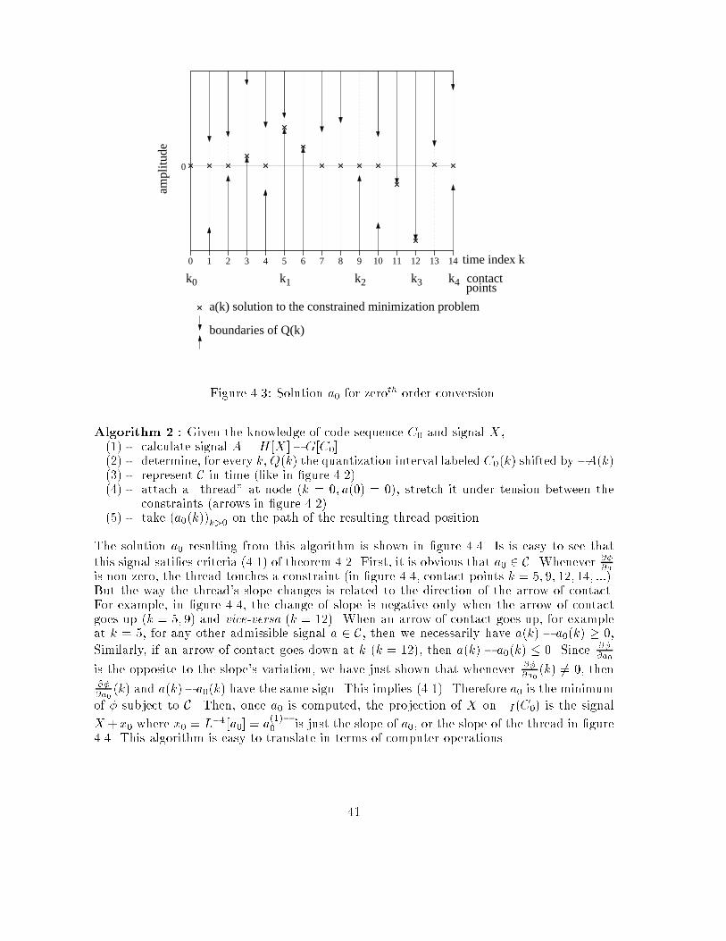
time index k0 654321 7 8 9 10 12 13 1411

contactk0 k1 k2 k3 k4

0

a(k) solution to the constrained minimization problem

boundaries of Q(k)

points

ampl

itude

Figure 4.3: Solution a0 for zeroth order conversion.Algorithm 2 : Given the knowledge of code sequence C0 and signal X ,(1) - calculate signal A = H [X ]� G[C0](2) - determine, for every k, Q(k) the quantization interval labeled C0(k) shifted by �A(k)(3) - represent C in time (like in �gure 4.2)(4) - attach a \thread" at node (k = 0; a(0) = 0), stretch it under tension between theconstraints (arrows in �gure 4.2)(5) - take (a0(k))k>0 on the path of the resulting thread position.The solution a0 resulting from this algorithm is shown in �gure 4.4. Is is easy to see thatthis signal sati�es criteria (4.1) of theorem 4.2. First, it is obvious that a0 2 C. Whenever @�@ais non zero, the thread touches a constraint (in �gure 4.4, contact points k = 5; 9; 12; 14; :::).But the way the thread's slope changes is related to the direction of the arrow of contact.For example, in �gure 4.4, the change of slope is negative only when the arrow of contactgoes up (k = 5; 9) and vice-versa (k = 12). When an arrow of contact goes up, for exampleat k = 5, for any other admissible signal a 2 C, then we necessarily have a(k)� a0(k) � 0,Similarly, if an arrow of contact goes down at k (k = 12), then a(k)� a0(k) � 0. Since @�@a0is the opposite to the slope's variation, we have just shown that whenever @�@a0 (k) 6= 0, then@�@a0 (k) and a(k)�a0(k) have the same sign. This implies (4.1). Therefore a0 is the minimumof � subject to C. Then, once a0 is computed, the projection of X on �I (C0) is the signalX+x0 where x0 = L�1[a0] = a(1)�0 is just the slope of a0, or the slope of the thread in �gure4.4. This algorithm is easy to translate in terms of computer operations.41

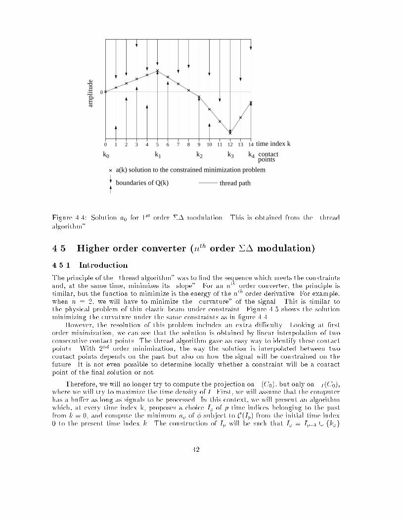
time index k0 654321 7 8 9 10 12 13 1411

contactk0 k1 k2 k3 k4

0

a(k) solution to the constrained minimization problem

boundaries of Q(k)

points

thread path

ampl

itude

Figure 4.4: Solution a0 for 1st order �� modulation. This is obtained from the \threadalgorithm".4.5 Higher order converter (nth order �� modulation)4.5.1 IntroductionThe principle of the \thread algorithm" was to �nd the sequence which meets the constraintsand, at the same time, minimizes its \slope". For an nth order converter, the principle issimilar, but the function to mimimize is the energy of the nth order derivative. For example,when n = 2, we will have to minimize the \curvature" of the signal. This is similar tothe physical problem of thin elastic beam under constraint. Figure 4.5 shows the solutionminimizing the curvature under the same constraints as in �gure 4.4.However, the resolution of this problem includes an extra di�culty. Looking at �rstorder minimization, we can see that the solution is obtained by linear interpolation of twoconsecutive contact points. The thread algorithm gave an easy way to identify these contactpoints. With 2nd order minimization, the way the solution is interpolated between twocontact points depends on the past but also on how the signal will be constrained on thefuture. It is not even possible to determine locally whether a constraint will be a contactpoint of the �nal solution or not.Therefore, we will no longer try to compute the projection on �(C0), but only on �I(C0),where we will try to maximize the time density of I . First, we will assume that the computerhas a bu�er as long as signals to be processed. In this context, we will present an algorithmwhich, at every time index k, proposes a choice Ip of p time indices belonging to the pastfrom k = 0, and compute the minimum ap of � subject to C(Ip) from the initial time index0 to the present time index k. The construction of Ip will be such that Ip = Ip�1 [ fkpg42

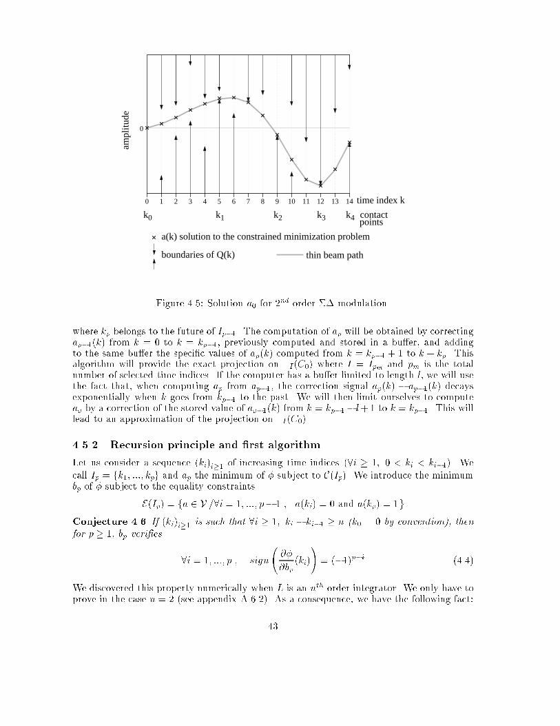
time index k0 654321 7 8 9 10 12 13 1411

contactk0 k1 k2 k3 k4

0

a(k) solution to the constrained minimization problem

boundaries of Q(k)

points

thin beam path

ampl

itude

Figure 4.5: Solution a0 for 2nd order �� modulation.where kp belongs to the future of Ip�1. The computation of ap will be obtained by correctingap�1(k) from k = 0 to k = kp�1, previously computed and stored in a bu�er, and addingto the same bu�er the speci�c values of ap(k) computed from k = kp�1 + 1 to k + kp. Thisalgorithm will provide the exact projection on �I(C0) where I = Ipm and pm is the totalnumber of selected time indices. If the computer has a bu�er limited to length l, we will usethe fact that, when computing ap from ap�1, the correction signal ap(k) � ap�1(k) decaysexponentially when k goes from kp�1 to the past. We will then limit ourselves to computeap by a correction of the stored value of ap�1(k) from k = kp�1� l+1 to k = kp�1. This willlead to an approximation of the projection on �I(C0).4.5.2 Recursion principle and �rst algorithmLet us consider a sequence (ki)i�1 of increasing time indices (8i � 1; 0 < ki < ki�1). Wecall Ip = fk1; :::; kpg and ap the minimum of � subject to C(Ip). We introduce the minimumbp of � subject to the equality constraintsE(Ip) = fa 2 V /8i = 1; :::; p� 1 ; a(ki) = 0 and a(kp) = 1gConjecture 4.6 If (ki)i�1 is such that 8i � 1; ki � ki�1 � n (k0 = 0 by convention), thenfor p � 1, bp veri�es 8i = 1; :::; p ; sign @�@bp (ki)! = (�1)p�i (4.4)We discovered this property numerically when L is an nth order integrator. We only have toprove in the case n = 2 (see appendix A.6.2). As a consequence, we have the following fact:43

Fact 4.7 We suppose that 8i � 1; ki � ki�1 � n (k0 = 0). If for a certain p � 2, ap�1veri�es(1) 8i = 1; :::; p� 1 ; sign � @�@ap�1 (ki)� = �(�1)p�i where � 2 f�1; 1g(2) ap�1(kp) is below (resp. above) interval Q(kp) when � = 1 (resp. �1)then ap veri�es(3) 8i = 1; :::; p ; sign � @�@ap (ki)� = �(�1)p�i(4) ap = ap�1 + ��bp, where � is the distance between ap�1(kp) and Q(kp)This is a consequence of (4.4), the Euler characterization, theorem 4.3 and the linearity ofa 7! @�@a (fact 4.5). The complete proof is shown in appendix A.3. This fact is still trueat p = 1, when taking a0 = 0 (zero signal). Of course the criteria (1) disappears becauseI0 = ;. Since � has not been determined yet, we will have the freedom to choose k1 suchthat 0 is either below or above Q(k1). Then � will be �xed to +1 or �1 respectively. Fact4.7 becomes:Fact 4.8 Assuming that k1 � n, if we have(2') 0 does not belong to Q(k1)then a1 veri�es(3') sign � @�@ap (ki)� = �, where � = 1 (resp. �1) if 0 is below (resp. above) Q(k1)(4') a1 = ��b1, where � is the distance of 0 to Q(k1)Proof : Like in the proof of fact 4.7 (A.3) one has to see that ��b1 2 C(I) and veri�es theEuler inequality with regard to C(I) 2These facts give us the foundation for our next algorithm. If we are able to �nd a set ofp� 1 increasing time indices Ip�1 = fk1; :::; kp�1g such that the minimum ap�1 of � subjectto C(Ip�1) can be obtained and veri�es criteria (1) of fact 4.7, then we will look for an indexkp � kp�1 + n such that criteria (2) is satis�ed. Taking Ip = Ip�1 \ fkpg, if we can calculatethe minimum bp of � subject to E(Ip), we can calculate the signal ap�1 + ��bp (where � and� are de�ned in criteria (1) and (4)) which is for sure the minimum ap of � subject to C(Ip).According to fact 4.7, ap veri�es criteria (3) which can be written:8i = 1; :::; p ; sign @�@ap (ki)! = (��)(�1)(p+1)�iand which is similar to criteria (1) when replacing p by p+ 1 and � by ��. At the �rst stepp = 1, the initial � is determined according to the choice of k1 and criteria (3'). We formallydescribe the algorithm as follows:Algorithm 3.1 : Given the knowledge of code sequence C0 and signal X ,(1) - Initialize p = 0, k0 = 0, I0 = ;, a0 = 0 (zero signal)(2) - Increment p(3) - For increasing k starting from kp�1 + n, determine Q(k) using the knowledge of C0and X (like in algorithm 2)(4) - Choose kp � kp�1+n such that ap�1(kp) is below (resp. above) Q(kp) if �0(�1)p = 1(resp. �1) (�0 is chosen at the same time as k1 during the �rst step p = 1)(5) - Calculate �p the distance between ap�1(kp) and Q(kp)(6) - Take Ip = Ip�1 \ fkpg(7) - Calculate the minimum bp of � subject to E(Ip)44

(8) - Calculate ap = ap�1 + �0(�1)p�pbp(9) - Go to (2)An example of construction of Ip; ap; bp according to this algorithm is shown in �gure 4.6.4.5.3 More practical version for algorithm 3.1One should not forget that the computation of ap is only an intermediate step in the com-putation of the projection X + xp of X on �Ip(C0): we still have to perform the operationxp = L�1[ap] = a(n)�p . If we apply the operator L�1 on the recursive relation of line (8) inalgorithm 3.1, we �nd xp = xp�1 + �0(�1)p�pypwhere yp = L�1[bp] = b(n)�p . However, line (4) of algorithm 3.1 still requires ap�1(k) to beknown for k > kp�1. Therefore, we will still need to determine bp�1(k) for k > kp. Wepropose the modi�ed algorithm:Algorithm 3.2 : In algorithm 3.1, replace lines (7) and (8) by(7) - Call bp the minimum of � subject to C(Ip)- calculate yp = b(n)�p- calculate bp(k) for k > kp(8) - - calculate xp = xp�1 + �0(�1)p�pyp- calculate ap(k) = ap�1(k) + �0(�1)p�pbp(k) for k > kp.This algorithm requires xp to be memorized at every step p. However, since xp is only anintermediate variable in the computation of the �nal solution xpm , it is not necessary todetermine xp explicitly on its full time range.Actually, xp is completely determined from the knowledge ofxp(1); x(1)+p (1); :::; x(n�1)+p ; and x(n)+p (ki) for i = 1; :::; pIndeed, as a consequence of theorem 4.3 and fact 4.5,8k =2 Ip; x(n)+p (k) = 0This implies that x(n)+p is known on the full time range and xp can be obtained from an nthorder integration of x(n)+p . But, when reaching the �nal step p = pm, xpm itself has to begiven explicitely: it is not realistic to compute it by an nth order integration from initialconditions given at k = 1 because of round o� error accumulation. Therefore, we propose anintermediate solution which consists in calculating the vectorsWp;i = 2664 x(n�2)+p (ki + 1)...x(0)+p (ki + 1) 3775 (4.5)for every i = 0; :::; p, to characterize xp. Indeed, xp can be reconstructed from (Wp;i)0�i�p�1using the following facts: 45

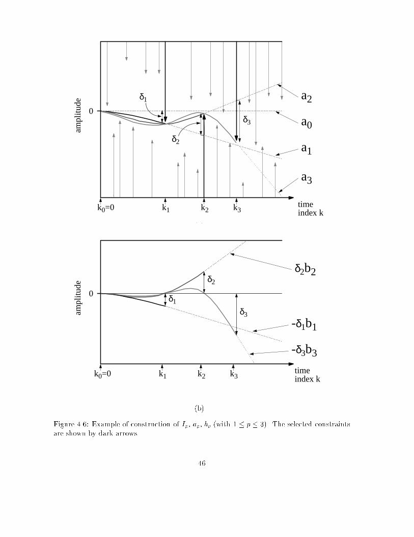
a2

a0

a1

a3

δ1

δ2

δ3

0

timeindex k

k1 k2 k3k0=0

ampl

itude

(a)0

timeindex k

k1 k2 k3k0=0

ampl

itude

δ1

δ2

δ3

-δ1b1

-δ3b3

δ2b2

(b)Figure 4.6: Example of construction of Ip, ap, bp (with 1 � p � 3). The selected constraintsare shown by dark arrows. 46

Fact 4.9 8k � kp + 1; 8q � 0; x(q)+p (k) = 0 and y(q)+p (k) = 0Proof : Suppose there exists h > kp such that xp(h) 6= 0. Let x0p the sequence equal to xpeverywhere except at k = h where x0p(h) = 0 and call a0p = L[x0p]. We have kx0pkV < kxpkVwhich implies �(a0p) < �(ap). Since L is causal, a0p will di�er from ap only for k � h. Thereforea0p 2 C(Ip) and �(a0p) � �(ap) which is impossible. We conclude that 8k > kp, xp(k) = 0. Itwill be also the case for its successive forward derivatives for k > kp. The reasoning is thesame for yp 2Fact 4.10 x(n�2)+p and y(n�2)+p are piecewise linear on intervals fki�1 + 1; :::; ki+ 1g (1 �i � p, k0 = 0).For 1 � i � p, 8k = ki�1 + 1; :::; ki � 1, x(n)+p (k) = 0, because of theorem 4.3 and fact4.5. Since x(n)+p (k) = (x(n�2)+p (k + 2)� x(n�2)+p (k + 1))� (x(n�2)+p (k + 1)� x(n�2)+p (k)), byde�nition of the forward derivative, we conclude that8k = ki�1+1; :::; ki� 1 ; (x(n�2)+p (k+2)� x(n�2)+p (k+1)) = (x(n�2)+p (k+1)� x(n�2)+p (k))Therefore, x(n�2)+ is piecewise linear on intervals fki�1 + 1; :::; ki + 1g. The reasoning issimilar for yp 2On every interval fki�1+ 1; :::; ki+ 1g, x(n�2)+p (k) can be obtained by linear interpolation ofthe top components of Wp;i�1 and Wp;i. Then, xp(k) can be obtained by an (n� 2)th orderintegration of x(n�2)+p on this interval, with initial conditions at k = ki�1 + 1 contained inWp;i�1. The length of integration will be this time limited to li = ki�ki�1. In the particularcase where i = p, note that Wp;p is the zero vector according to fact 4.9. This fact also saysthat xp(k) does not need to be calculated for k � kp + 1 since it is necessarily equal to zero.From line (4) of algorithm 3.2, we need to determine ap(k) at least for k � kp + n.From fact 4.9 we have a(n)�p (k) = xp(k) = 0 for k � kp + 1. This implies that ap(k) can bedetermined by an nth order integration of the zero signal on k � kp + 1, provided we knowthe initial conditions at k = kp: ap(kp); a(1)�p (kp); :::; a(n�1)�p (kp). For this purpose, we de�nethe following vector Vp = 2664 a(n�1)�p (kp)...a(1)�p (kp) 3775 (4.6)We will call Wp;i; Vp the vectors associated with ap. They all have size (n� 1). Note that inthe case n = 2, they are just scalars. Similarly, let us de�ne W 0p;i; V 0p the vectors associatedwith bp as W 0p;i = 2664 y(n�2)+p (ki + 1)...y(0)+p (ki + 1) 3775 (0 � i � p) and V 0p = 2664 b(n�1)�p (kp)...b(1)�p (kp) 3775 (4.7)Algorithm 3.2 becomes 47

Algorithm 3.3 : In algorithm 3.2, replace lines (1),(3),(4),(7) and (8) by(1) - Initialize p = 0, k0 = 0, I0 = ;, a0(0) = 0, V0 = On�1 (null vector of size n � 1)(3) - For increasing k starting from kp�1 + 1, determine- Q(k) using the knowledge of C0 and X (like in algorithm 2)- ap�1(k) by nth order integration of the zero signal with initial conditions at k = kp�1given by ap�1(kp�1) and Vp�1(4) - Choose kp � kp�1+n such that ap�1(kp) is below (resp. above) Q(kp) if �0(�1)p = 1(resp. �1) (�0 is chosen at the same time as k1 during the �rst step p = 1)Call V 0p�1 = ha(n�1)�p�1 (kp) � � �a(1)�p�1 (kp)iT(7) - Calculate (W 0p;i)0�i�p�1; V 0p the vectors associated with the minimum bp of � subjectto C(Ip) (see formula (4.7))(8) - CalculateWp;i = Wp�1;i + �0(�1)p�pW 0p;i , for 0 � i � p� 2Wp;p�1 = �0(�1)p�pW 0p;p�1Vp = V 0p�1 + �0(�1)p�pV 0pap(kp) = ap�1(kp) + �0(�1)p�pLine (8) requires (W 0p;i)0�i�p�1 to be memorized for the next step (p+ 1).4.5.4 Computation of W 0p;i; V 0pWe show in this section that W 0p;i and V 0p can be calculated algebraically from the recursivecomputation of a (2n� 2)� (n� 1) matrix Rp and a p(n� 1)� (n� 1) matrixMp. We �rstintroduce some notation:Notation 4.11 For any sequence b 2 V, we de�ne the column vectorUb(k) = hy(n�2)+(k + 1) � � �y(0)+(k + 1) b(n�1)�(k) � � �b(1)�(k)iTwhere k 2 N and y = b(n)� (by convention for any q � 0, b(q)�(0) = 0).We have the following preliminary fact:Fact 4.12 Let k � 1, l � n be two integers, and b 2 V such that 8h = 1; :::; l, y(n)+(k+h) = 0where y = b(n)�. Then Ub(k+ l) is uniquely determined by Ub(k), b(k) and b(k+ l) as follows:Ub(k + l) =M(l)Ub(k) +N(l)(b(k+ l)� b(k))where M(l) is a (2n � 2) square matrix and N(l) a (n � 1) column vector, both functionsof the integer variable l. The expressions of M(l) and N(l) as functions of l, are given inappendix A.4.3.For the sequence (ki)1�i�p , let us denote li = ki � ki�1 with the convention k0 = 0.Notation 4.13 P and Q are the two (n�1)�(2n�2) matrices P = [In�1;n�1jOn�1;n�1] andQ = [On�1;n�1jIn�1;n�1], where In�1;n�1 and On�1;n�1 are respectively the (n� 1)2 identityand null matrices. 48

Fact 4.14 Let (Ri)0�i�p and (Mi)0�i�p be the matrix sequences recursively de�ned by( R0 = PTM0 = [ ] and 8i = 1; :::; p ; 8><>: Ri =M(li)Ri�1Mi = " Mi�1PRi�1 # (4.8)Then the matrix PRp is invertible and (W 0p;i)0�i�p�1 and V 0p can be expressed in terms of Rpand Mp as follows: 2664 W 0p;0...W 0p;p�1 3775 = �Mp(PRp)�1PN(lp) (4.9)V 0p = �Q� (QRp)(PRp)�1P�N(lp) (4.10)We study in detail the case n = 2 in appendix A.64.5.5 RecapitulationWith the resolution of W 0p;i; V 0p , algorithm 3.3 becomesAlgorithm 3.4 : In algorithm 3.3, replace lines (1) and (7) by(1) Initialize p = 0, k0 = 0, I0 = ;, a0(0) = 0, V0 = On�1, R0 = PT , M0 = [ ](7.1) - Call lp = kp � kp�1(7.2) - Take Rp =M(lp)Rp�1 and Mp = " Mp�1PRp�1 #(7.3) - Calculate 2664 W 0p;0...W 0p;p�1 3775 = �Mp(PRp)�1PN(lp)and V 0p = �Q� (QRp)(PRp)�1P �N(lp)This requires the inversion of a square matrix (PRp) of size (n � 1)2 at every iteration p.Note that in the case n = 2, this is just a scalar inversion. We also see that line (7.3) requiresthe memorization of the growing matrixMp of size p(n�1)�(n�1). We saw in the previoussection that (W 0p;i)0�i�p�1 had to be memorized as well (equivalent to a column vector of sizep(n� 1).The inversion of PRp in relations (4.9) and (4.10) can lead to numerical di�culties asRp is a matrix growing with p (see relation (4.8)). This problem can be solved with thefollowing fact:Fact 4.15 Formulas (4.9) and (4.10) are still true with the matrix sequences (Ri)0�i�p and(Mi)0�i�p recursively de�ned by( R0 = PTM0 = [ ] and 8i = 1; :::; p ; 8><>: Ri =M(li)Ri�1TiMi = " Mi�1PRi�1 #Ti (4.11)where (Ti)0�i�p is an arbitrary sequence of invertible matrices of size (n� 1).49

This leads to an algorithm with more computation freedom then algorithm 3.4Algoritm 3.5 : In algorithm 3.4, replace line (7.2) by(7.2) - Choose an (n� 1) invertible matrix TpTake Rp =M(lp)Rp�1Tp and Mp = " Mp�1PRp�1 #TpAlgorithm 3.4 will simply be the particular case of 3.5 where Tp is systematically taken equalto the identity matrix.We propose a particular choice of Tp to make the inversion of PRp practical. At step p,let UpSpVTp be the singular value decomposition of M(lp)Rp�1, whereUp is an (2n� 2)� (n � 1) matrix with orthonormal column vectors,Sp is an (n� 1)2 invertible diagonal matrixVp is an (n� 1)2 orthogonal matrix.If we take Tp = VpS�1p , we will have Rp = (UpSpVTp )(VpS�1p ) = Up. The inversion ofPRp = PUp thus becomes well conditioned. For this choice of Tp, algorithm 3.5 has theparticular form:Algorithm 3.6 : In algorithm 3.5, replace line (7.2) by(7.2) - Perform the singular value decomposition UpSpVTp of M(lp)Rp�1Take Rp = Up and Mp = " Mp�1PRp�1 #VpS�1p4.5.6 Algorithms 3.4, 3.5 with limited bu�erFrom the recursive relation of line (8) in algorithm 3.4 or 3.5, it can be derived that8q � i+ 1; Wq;i = qXp=i+2 (Wp;i �Wp�1;i) +Wi+1;i = �0 qXp=i+1(�1)p�pW 0p;iSuppose pm is the �nal number of selected indices. Then, the vectors associated with the�nal solution xpm are Wpm;i = �0 pmXp=i+1(�1)p�pW 0p;i for 0 � i � pm (4.12)We show in appendix A.6.3 that, in the case n = 2, W 0p;i decays exponentially for a �xed iand increasing p. We also observed numerically this behavior for higher orders n. It can bedecided that a predetermined number l0 of terms in the summation of (4.12) is enough togive a good approximation of Wpm;iWpm;i ' �0 i+l0Xp=i+1(�1)p�pW 0p;i = Wi+l0;i (4.13)In other words, every Wp;i produced by line (8) should be output as soon as p � i + l0 ori � p� l0. This implies that only hWp;p�(l0�1) � � �Wp;p�1i will be needed and kept in memory50

for the next iteration step (p+ 1). This requires a bu�er of length (l0 � 1)(n� 1). Anotherconsequence is that, at step p, hW 0p;p�l0 � � �W 0p;p�1i are the only values needed from line (7)of algorithm 3.4 or 3.5. This means that, in line (7.3), only the last l0(n � 1) rows of Mpneed to be known. Therefore, this requires the memorization of the last (l0� 1)(n� 1) rowsof Mp�1 from the previous step (p� 1) for the calculation of line (7.2) at step p. Since therows of Mp�1 have length (n� 1), this requires a bu�er of length (l0 � 1)(n� 1)� (n � 1).In total, we need a bu�er of size (l0 � 1)n(n� 1).Conversely, if we have a bu�er with a size limited to s, then the number of terms in theapproximation (4.13) will be the integer part of sn(n�1) + 1.

51

Chapter 5Numerical experimentsWe performed numerical tests to both verify our analytical evaluation of the MSE and val-idate our projection algorithms. For convenience, but also to keep the same conditions ofsignal coding as in chapter 3, we dealt with periodic input signals. We actually reduced thecomplexity of input signals to sinusoids.We draw X0 at random in the Fourier domain and then perform an inverse DFT fordi�erent oversampling rates (M > 2N + 1). After calculating the code sequence C0 of X0through a �xed A/D converter, we measure the MSE betweenX0 and the estimateX obtainedby alternate projections. We repeat this operation on a certain number of drawn signals(300 to 1000) and calculate the statistical average of the MSE. We know that alternatingprojections on convex sets converges theoretically to their intersection. In practice, however,we have to limit the number of iterations to only obtain an approximation of an element inV0 \ �(C0).5.1 Validation of the R�(2n+2) behavior of the MSE with si-nusoidal inputsWorking with sinusoidal inputs, we con�rm that the expectation of MSE(X0; X) decreaseswith R proportionally to R�(2n+2), where n is the order of the circuit. In �gure 5.1 and 5.2,we show the comparison of performance in SNR between the classical reconstruction andthe alternate projection method. We represent the SNR in dB, where the reference (0dB)corresponds to an MSE equal to q212 (variance of a random signal with a uniform distributionin [�12 ; 12 ]). For classical reconstruction SNR, we used the theoretical formula in [2] givingthe in-band noise power for an nth order converter, assuming that the quantization errorsignal is uncorrelated in time: �2n2n+ 1 � �2qR2n+1 (5.1)where �2q is the variance of the quantization error power. For the alternate projection method,since we want to �nd an estimate as close as possible to V0\�(C0) to validate our theoreticalevaluation of MSE, we stop the iteration process as soon as the relative increment of SNRbecomes less than 0.01 dB.For the case n = 0, we considered simple ADC with uniform quantization and inputsignals of peak-to peak amplitude equal to 2q and random dc component, where q is the step52

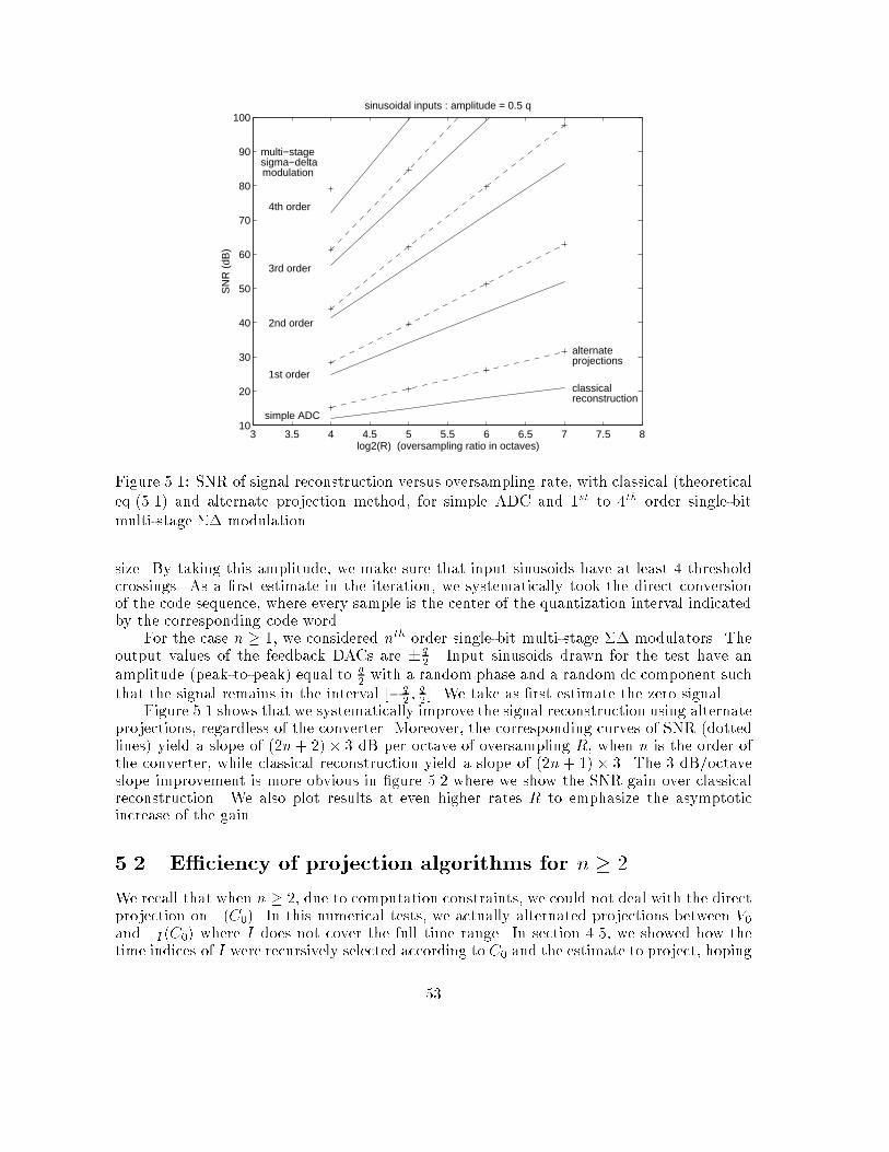
3 3.5 4 4.5 5 5.5 6 6.5 7 7.5 810

20

30

40

50

60

70

80

90

100

log2(R) (oversampling ratio in octaves)

SN

R (

dB)

sinusoidal inputs : amplitude = 0.5 q

classicalreconstruction

alternateprojections

simple ADC

1st order

2nd order

3rd order

4th order

multi−stagesigma−deltamodulation

Figure 5.1: SNR of signal reconstruction versus oversampling rate, with classical (theoreticaleq.(5.1) and alternate projection method, for simple ADC and 1st to 4th order single-bitmulti-stage �� modulation.size. By taking this amplitude, we make sure that input sinusoids have at least 4 thresholdcrossings. As a �rst estimate in the iteration, we systematically took the direct conversionof the code sequence, where every sample is the center of the quantization interval indicatedby the corresponding code word.For the case n � 1, we considered nth order single-bit multi-stage �� modulators. Theoutput values of the feedback DACs are � q2 . Input sinusoids drawn for the test have anamplitude (peak-to-peak) equal to q2 with a random phase and a random dc component suchthat the signal remains in the interval [� q2 ; q2 ]. We take as �rst estimate the zero signal.Figure 5.1 shows that we systematically improve the signal reconstruction using alternateprojections, regardless of the converter. Moreover, the corresponding curves of SNR (dottedlines) yield a slope of (2n+ 2)� 3 dB per octave of oversampling R, when n is the order ofthe converter, while classical reconstruction yield a slope of (2n+ 1)� 3. The 3 dB/octaveslope improvement is more obvious in �gure 5.2 where we show the SNR gain over classicalreconstruction. We also plot results at even higher rates R to emphasize the asymptoticincrease of the gain.5.2 E�ciency of projection algorithms for n � 2We recall that when n � 2, due to computation constraints, we could not deal with the directprojection on �(C0). In this numerical tests, we actually alternated projections between V0and �I (C0) where I does not cover the full time range. In section 4.5, we showed how thetime indices of I were recursively selected according to C0 and the estimate to project, hoping53

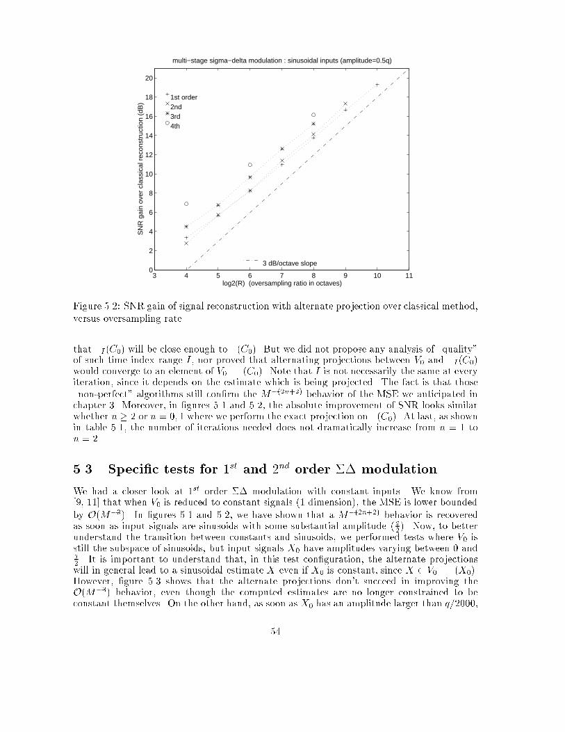
3 4 5 6 7 8 9 10 110

2

4

6

8

10

12

14

16

18

20

multi−stage sigma−delta modulation : sinusoidal inputs (amplitude=0.5q)

log2(R) (oversampling ratio in octaves)

SN

R g

ain

over

cla

ssic

al r

econ

stru

ctio

n (d

B)

1st order2nd3rd4th

3 dB/octave slopeFigure 5.2: SNR gain of signal reconstruction with alternate projection over classical method,versus oversampling rate.that �I (C0) will be close enough to �(C0). But we did not propose any analysis of \quality"of such time index range I , nor proved that alternating projections between V0 and �I (C0)would converge to an element of V0\�(C0). Note that I is not necessarily the same at everyiteration, since it depends on the estimate which is being projected. The fact is that those\non-perfect" algorithms still con�rm the M�(2n+2) behavior of the MSE we anticipated inchapter 3. Moreover, in �gures 5.1 and 5.2, the absolute improvement of SNR looks similarwhether n � 2 or n = 0; 1 where we perform the exact projection on �(C0). At last, as shownin table 5.1, the number of iterations needed does not dramatically increase from n = 1 ton = 2.5.3 Speci�c tests for 1st and 2nd order �� modulationWe had a closer look at 1st order �� modulation with constant inputs. We know from[9, 11] that when V0 is reduced to constant signals (1 dimension), the MSE is lower boundedby O(M�3). In �gures 5.1 and 5.2, we have shown that a M�(2n+2) behavior is recoveredas soon as input signals are sinusoids with some substantial amplitude ( q2). Now, to betterunderstand the transition between constants and sinusoids, we performed tests where V0 isstill the subspace of sinusoids, but input signals X0 have amplitudes varying between 0 andq2 . It is important to understand that, in this test con�guration, the alternate projectionswill in general lead to a sinusoidal estimate X even if X0 is constant, since X 2 V0 \ �(X0).However, �gure 5.3 shows that the alternate projections don't succeed in improving theO(M�3) behavior, even though the computed estimates are no longer constrained to beconstant themselves. On the other hand, as soon as X0 has an amplitude larger than q=2000,54

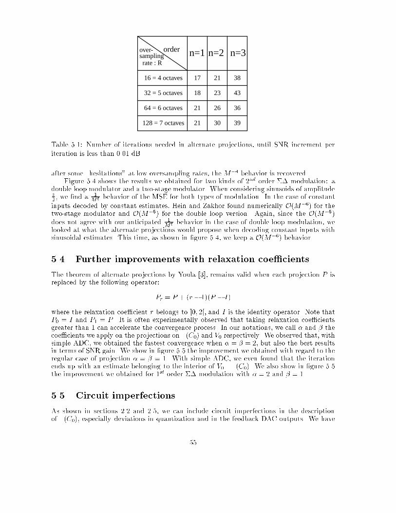
17

n=3n=2n=1over-samplingrate : R

16 = 4 octaves

32 = 5 octaves

64 = 6 octaves

128 = 7 octaves

21 38

18 23 43

21 26 36

30 39 21

order

Table 5.1: Number of iterations needed in alternate projections, until SNR increment periteration is less than 0.01 dB.after some \hesitations" at low oversampling rates, the M�4 behavior is recovered.Figure 5.4 shows the results we obtained for two kinds of 2nd order �� modulation: adouble loop modulator and a two-stage modulator. When considering sinusoids of amplitudeq2 , we �nd a 1M6 behavior of the MSE for both types of modulation. In the case of constantinputs decoded by constant estimates, Hein and Zakhor found numerically O(M�6) for thetwo-stage modulator and O(M�5) for the double loop version. Again, since the O(M�5)does not agree with our anticipated 1M6 behavior in the case of double loop modulation, welooked at what the alternate projections would propose when decoding constant inputs withsinusoidal estimates. This time, as shown in �gure 5.4, we keep a O(M�6) behavior.5.4 Further improvements with relaxation coe�cientsThe theorem of alternate projections by Youla [3], remains valid when each projection P isreplaced by the following operator:Pr = P + (r � 1)(P � I)where the relaxation coe�cient r belongs to ]0; 2[, and I is the identity operator. Note thatP0 = I and P1 = P . It is often experimentally observed that taking relaxation coe�cientsgreater than 1 can accelerate the convergence process. In our notations, we call � and � thecoe�cients we apply on the projections on �(C0) and V0 respectively. We observed that, withsimple ADC, we obtained the fastest convergence when � = � = 2, but also the best resultsin terms of SNR gain. We show in �gure 5.5 the improvement we obtained with regard to theregular case of projection � = � = 1. With simple ADC, we even found that the iterationends up with an estimate belonging to the interior of V0 \ �(C0). We also show in �gure 5.5the improvement we obtained for 1st order �� modulation with � = 2 and � = 1.5.5 Circuit imperfectionsAs shown in sections 2.2 and 2.5, we can include circuit imperfections in the descriptionof �(C0), especially deviations in quantization and in the feedback DAC outputs. We have55

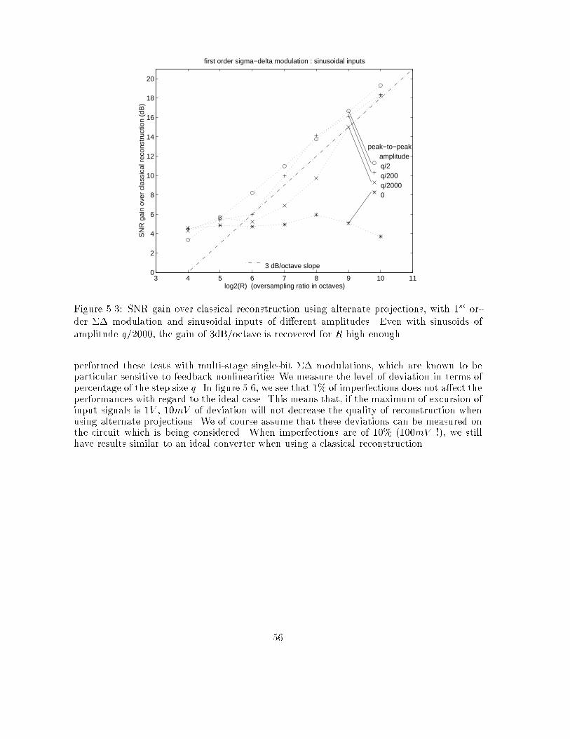
3 4 5 6 7 8 9 10 110

2

4

6

8

10

12

14

16

18

20

first order sigma−delta modulation : sinusoidal inputs

log2(R) (oversampling ratio in octaves)

SN

R g

ain

over

cla

ssic

al r

econ

stru

ctio

n (d

B)

peak−to−peak amplitudeq/2q/200q/20000

3 dB/octave slopeFigure 5.3: SNR gain over classical reconstruction using alternate projections, with 1st or-der �� modulation and sinusoidal inputs of di�erent amplitudes. Even with sinusoids ofamplitude q=2000, the gain of 3dB/octave is recovered for R high enough.performed these tests with multi-stage single-bit �� modulations, which are known to beparticular sensitive to feedback nonlinearities We measure the level of deviation in terms ofpercentage of the step size q. In �gure 5.6, we see that 1% of imperfections does not a�ect theperformances with regard to the ideal case. This means that, if the maximum of excursion ofinput signals is 1V , 10mV of deviation will not decrease the quality of reconstruction whenusing alternate projections. We of course assume that these deviations can be measured onthe circuit which is being considered. When imperfections are of 10% (100mV !), we stillhave results similar to an ideal converter when using a classical reconstruction.56

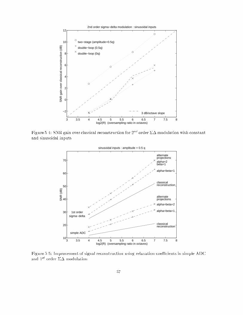
3 3.5 4 4.5 5 5.5 6 6.5 7 7.5 8

−2

0

2

4

6

8

10

122nd order sigma−delta modulation : sinusoidal inputs

log2(R) (oversampling ratio in octaves)

SN

R g

ain

over

cla

ssic

al r

econ

stru

ctio

n (d

B)

two−stage (amplitude=0.5q)

double−loop (0.5q)

double−loop (0q)

3 dB/octave slopeFigure 5.4: SNR gain over classical reconstruction for 2nd order ��modulation with constantand sinusoidal inputs.3 3.5 4 4.5 5 5.5 6 6.5 7 7.5 8

10

20

30

40

50

60

70

log2(R) (oversampling ratio in octaves)

SN

R (

dB)

sinusoidal inputs : amplitude = 0.5 q

classicalreconstruction

classicalreconstruction

alternateprojections

alpha=beta=2

alpha=beta=1

alternateprojectionsalpha=2beta=1

alpha=beta=1

simple ADC

1st ordersigma−deltaFigure 5.5: Improvement of signal reconstruction using relaxation coe�cients in simple ADCand 1st order �� modulation. 57

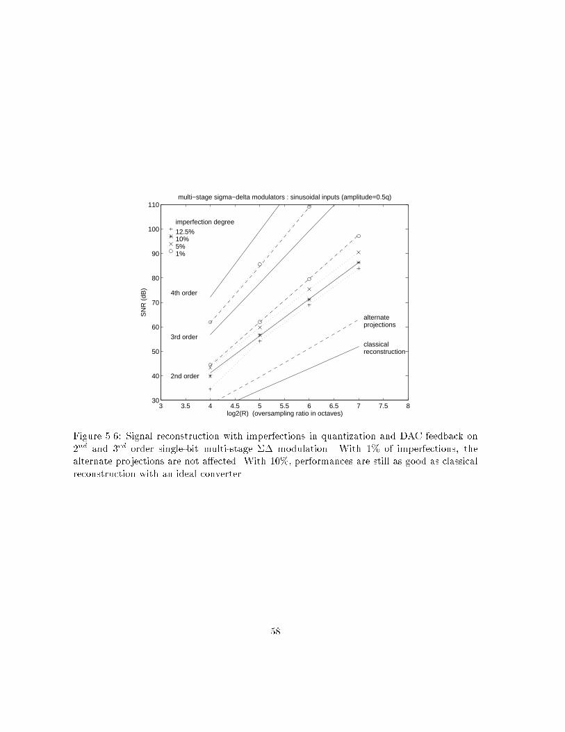
3 3.5 4 4.5 5 5.5 6 6.5 7 7.5 830

40

50

60

70

80

90

100

110

log2(R) (oversampling ratio in octaves)

SN

R (

dB)

multi−stage sigma−delta modulators : sinusoidal inputs (amplitude=0.5q)

imperfection degree

12.5%10%5%1%

classicalreconstruction

alternateprojections

2nd order

3rd order

4th order

Figure 5.6: Signal reconstruction with imperfections in quantization and DAC feedback on2nd and 3rd order single-bit multi-stage �� modulation. With 1% of imperfections, thealternate projections are not a�ected. With 10%, performances are still as good as classicalreconstruction with an ideal converter.58

Appendix AAppendixA.1 Proof lemmas 3.2 and 3.5For simplicity, we suppose that the period T0 of input signals is equal to 1 (the time dimensioncan always be rescaled). To prove lemmas 3.2 and 3.5, the idea is to see that V (k)Mn can beuniformly approximated by by the nth order integral U (�n)[t] of U [t] taken at time t = kM .This approximation will be expressed in lemmas A.2 (n = 1) and lemma A.5 (n � 1). Thenthe maximum value and the average of jV (k)j will be approximated by the in�nite and theL1 norms, respectively, of this integral. The upper and lower bounds will be then derivedfrom norm equivalence (lemma A.6).A.1.1 Preliminary notations and lemmasNotation A.1 Norms k � k1 and k � k1For a continuous function f on [0; 1], kfk1 = maxt2[0;1] jf [t]j and kfk1 = Z 10 jf [t]jdt.Lemma A.2 Let f be a function C1 on [0; 1]. Then 8M � 1; 8k = 1; :::;M ,������ 1M kXj=1 f [ jM ]� Z kM0 f [t]dt������ � 1M kf 0k1 (A.1)������ 1M kXj=1 ���f [ jM ]���� Z kM0 jf [t]jdt������ � 1M kf 0k1 (A.2)This is proved in A.1.4. We are going to generalize this lemma to higher order integration.We �rst introduce some notation for the nth order continuous time and discrete integration.Notation A.3 nth order derivative and integralFor a function F , C1 on [0; 1], and an integer n � 0, f (n) designates the nth order derivativeand f (�n) is the nth order integral which is equal to 0 at t = 0. More precisely, f (0) = f andfor n � 1, f (�n) is the integral of f (�n+1) which is equal to 0 at t = 0.59

Notation A.4 nth order discrete sumFor a function f de�ned on [0; 1], and an integer M � 1, Inf;M is the M -point sequencede�ned recursively as follows8k = 1; :::;M; I0f;M(k) = f [ kM ] and for n � 1; 8k = 1; :::;M; Inf;M(k) = kXj=1 In�1f;M (j)Lemma A.5 Let f be a function C1 on [0; 1] and n � 0 an integer.8M � 1; 8k = 1; :::;M; ������ 1Mn kXj=1 Inf;M(j)� Z kM0 f (�n)[t]dt������ � 1M 1Xm=�n+1 f (m) 1 (A.3)8M � 1; 8k = 1; :::;M; ������ 1Mn kXj=1 ���Inf;M(j)���� Z kM0 ���f (�n)[t]���dt������ � 1M 1Xm=�n+1 f (m) 1(A.4)This is proved in A.1.5.Remark : Replacing n by n� 1, (A.3) can be rewritten8M � 1; 8k = 1; :::;M; ���� 1Mn Inf;M(k)� f (�n)[ kM ]���� � 1M 1Xm=�n+2 f (m) 1 (A.5)We recall that S is the unit sphere of V0: S = nU 2 V0 . k~Uk = 1oLemma A.6 Let N be a norm on V0 and n 2 Z. Then9B+ > 0; 8U 2 S; N �U (n)� � B+ (A.6)If moreover n � 0, then 9B� > 0; 8U 2 S; N �U (n)� � B� (A.7)Proof : Properties of �nite dimensional normed spaces 2A.1.2 Proof of lemma 3.2By de�nition of L, we have exactly V (k) = InU;M(k) for k = 1; :::;M . If we apply (A.5) onf = U , we �nd8M � 1; 8k = 1; :::;M; ����V (k)Mn � U (�n)[ kM ]���� � 1M 1Xm=�n+2 U (m) 1 (A.8)Let t0 2 [0; 1] be the instant when ���U (�n)[t]��� achieves its maximum. We have���U (�n)[t0]��� = U (�n) 160

For k 2 f1; :::;Mg, using Lagrange inequality between kM and t0, we �nd���U (�n)[ kM ]� U (�n) 1��� � j kM � t0j U (�n+1) 1Together with (A.8), we �nd that 8M � 1; 8k = 1; :::;M ,����V (k)Mn � U (�n) 1���� � j kM � t0j U (�n+1) 1 + 1M 1Xm=�n+2 U (m) 1 (A.9)Since j kM � t0j � 1 and 1M � 1, this immediately gives an upper bound to ���V (k)Mn ��� :����V (k)Mn ���� � U (�n) 1 + U (�n+1) 1 + 1Xm=�n+2 U (m) 1 = 1Xm=�n U (m) 1This last term can be bounded by a constant c2 > 0, according to relation (A.6) of lemmaA.6. This proves that max1�k�M jV (k)j � c2MnInequality (A.9) also implies that����V (k)Mn ���� � U (�n) 1 � j kM � t0j U (�n+1) 1 � 1M 1Xm=�n+2 U (m) 1For everyM � 1, it is always possible to �nd kM 2 f1; :::;Mg such that jkMM � t0j � 1M . Thenmax1�k�M ����V (k)Mn ���� � ����V (kM)Mn ���� � U (�n) 1 � 1M 1Xm=�n+1 U (m) 1From relation (A.7) of lemma A.6, we can �nd B1 > 0 such that U (�n) 1 � B1. Fromrelation (A.6), we can �nd B2 > 0 such that1Xm=�n+1 U (m) 1 � B2 (A.10)As soon as M � 2B2B1 then max1�k�M ����V (k)Mn ���� � B1 � B2M � B12Taking c1 = B12 , then we have shown that when M is large enoughmax1�k�M jV (k)j � c1Mn 261

A.1.3 Proof of lemma 3.5Applying (A.4) with f = U and k =M , we �nd������ 1M MXj=1 ����V (k)Mn ����� U (�n) 1������ � 1M 1Xm=�n+1 U (m) 1 (A.11)According to (A.10), we can bound the right hand side by B2M . Consequently, U (�n) 1 � B2M � 1M MXj=1 ����V (k)Mn ���� � U (�n) 1 + B2M (A.12)Applying property (A.7) of lemma A.6, it is possible to �nd constants 0 < B� < B+ suchthat B� � kU (�n)k1 � B+The right hand side of (A.12) can be bounded by c4 = B+ + B2. Then for any M � B22B� ,the left hand side of (A.12) can be lower bounded byc3 = B� � � B22B���1B2 = B�2 > 0 2A.1.4 Proof of lemma A.2Let us consider integers M � 1 and k 2 f1; :::;Mg.Since f is continuous8j = 1; :::; k; 9tj 2 h j�1M ; jM i ; Z jMj�1M f [t]dt = 1M f [tj ]Then1M kXj=1 f [ jM ]� Z kM0 f [t]dt = kXj=1 1M f [ jM ]� Z jMj�1M f [t]dt! = 1M kXj=1 �f [ jM ]� f [tj ]� (A.13)Since jf j is also continuous, we can derive in a similar way that8j = 1; :::; k; 9t0j 2 hj�1M ; jM i ; 1M kXj=1 ���f [ jM ]���� Z kM0 jf [t]jdt = 1M kXj=1 ����f [ jM ]���� ���f [t0j ]����(A.14)For a �xed j 2 f1; :::; kg, 8t 2 hj�1M ; jM i������f [ jM ]���� jf [t]j��� � ���f [ jM ]� f [t]��� � ��� jM � t��� maxs2[t; jM ] jf 0[s]j! � 1M kf 0k1Therefore, since k � M , both expressions (A.13) and (A.14) can be bounded in absolutevalue by 1M kf 0k1 2 62

A.1.5 Proof of lemma A.5For a �xed integer M � 1, let us introduce the propositionP(n) : \ 8k = 1; :::;M; ������ 1Mn+1 kXj=1 Inf;M(j)� Z kM0 f (�n)[t]dt������ � 1M 1Xm=�n+1 f (m) 1 "Let us show P(n) by induction. P(0) is just the expression of lemma A.2. Suppose now thatP(n� 1) is true for a certain n � 1. Using the fact thatInf;M(j) = jXi=1 In�1f;M (i) and f (�n)[ jM ] = Z jM0 f (�n+1)[t]dt (A.15)we can write1Mn+1 kXj=1 Inf;M(j)� Z kM0 f (�n)[t]dt = 1M kXj=10@ 1Mn jXi=1 In�1f;M (i)� Z jM0 f (�n+1)[t]dt1A+0@ 1M kXj=1 f (�n)[ jM ]� Z kM0 f (�n)[t]dt1A (A.16)Applying the fact that P(n� 1) is true, we �nd1M kXj=1 ������ 1Mn jXi=1 In�1f;M (i)� Z jM0 f (�n+1)[t]dt������ � kM2 1Xm=�n+2 f (m) 1 � 1M 1Xm=�n+2 f (m) 1(A.17)Then applying (A.1) on function f (�n) which is C1, we �nd������ 1M kXj=1 f (�n)[ jM ]� Z kM0 f (�n)[t]dt������ � 1M f (�n+1) 1 (A.18)P(n) is then a consequence of (A.16),(A.17) and (A.18). The induction is completed: P(n)is true for every n � 0.To show (A.4), we write an equation similar to (A.16), using (A.15)1Mn+1 kXj=1 ���Inf;M(j)���� Z kM0 ���f (�n)[t]��� dt = 1M kXj=10@ 1Mn ������ jXi=1 In�1f;M (i)������� �����Z jM0 f (�n+1)[t]dt�����1A+0@ 1M kXj=1 ���f (�n)[ jM ]���� Z kM0 ���f (n)[t]���dt1AUsing the inequality jjaj � jbjj � ja�bj and applying P(n�1), the �rst term can be boundedin absolute value like in (A.17). The second term can be bounded by 1M f (�n+1) 1 byapplying (A.2) on f (�n) 2 63

A.2 Proof of fact 4.5LetD(n)� andD(n)+ be the linear and time invariant operators whose z transforms are (1�z�1)nand (z � 1)n. For two given sequences a and x, let �a and �x be their respective extension tonegative time indices: 8k � 1; �a(k) = a(k) and �x(k) = x(k)8k � 0; �a(k) = �x(k) = 0It can be veri�ed that a(n)� and x(n)+ are the restriction to N� of D(n)� [�a] and D(n)+ [�x]. Letd(n)� and d(n)+ be the impulse responses of D(n)� and D(n)+ . We have8j � 1; a(n)�(j) = �d(n)� � �a� (j) = +1Xk=1 d(n)� (k� j)a(k) (A.19)8k � 1; x(n)+(k) = �d(n)+ � �x� (k) = +1Xj=1 d(n)+ (j � k)x(j) (A.20)Suppose that x = L�1[a] = a(n)�. Then �(a) = 12Pj�1 jx(j)j2 and@�@a (k) = 12 +1Xj=1 @jx(j)j2@a(k) = +1Xj=1 @x(j)@a(k)x(j) (A.21)Using (A.19), we have @x(j)@a(k) = @a(n)�(j)@a(k) = d(n)� (k � j) (A.22)Since the z transforms of D(n)� and D(n)+ verify D(n)� (z) = (�1)nD(n)+ (z�1), then8k 2 Z; d(n)� (k) = (�1)nd(n)+ (�k) (A.23)Using successively (A.21), (A.22), (A.23) and (A.20) we �nd@�@a (k) = +1Xj=1 d(n)� (k � j)x(j) = (�1)n +1Xj=1 d(n)+ (j � k)x(j) = (�1)nx(n)+(k) 2A.3 Proof of fact 4.7Using Euler characterization and unicity of the minimum, we are going to show thats0 = ap�1 + ��bpis necessarily the minimum of � subject to C(Ip).First, we have to check that s0 2 C(Ip). We use the fact that8i = 1; :::; p� 1 ; bp(ki) = 0 and bp(kp) = 164

This implies that s0(ki) = ap�1(ki) 2 Q(ki), since ap�1 2 C(Ip�1). We also �nd thats0(kp) = ap�1(kp) + ��. Using assumption (2) on ap�1 and the de�nition of � in (4), weconclude that s0(kp) is the closest bound of Q(kp) to ap�1(kp) (A.24)Therefore s0(kp) 2 Q(kp).Let us now show that the Euler inequality characterization is satis�ed by s0 with regardto C(Ip).From fact 4.5, we can see that a 7! @�@a is linear. Therefore@�@s0 = @�@ap�1 + �� @�@bp (A.25)Using the fact that C(Ip�1) and E(Ip) are separable constraints and using theorem 4.3, we�nd that 8k =2 Ip�1; @�@ap�1 (k) = 0 (A.26)8k =2 Ip; @�@bp (k) = 0 (A.27)Since Ip � Ip�1, this implies that 8k =2 Ip; @�@s0 (k) = 0 (A.28)Let us now study the sign of @�@s0 (k) � (a(k)� s0(k)) when k 2 Ip and a 2 C(Ip).We �rst consider the case k = kp. Applying (A.26) and (4.4) at k = kp, we �nd@�@ap�1 (kp) = 0 and @�@bp (kp) � 0. From (A.25), this implies that @�@s0 (kp) = �� @�@bp (kp) andtherefore sign� @�@s0 (kp)� = � (A.29)For any r 2 Q(kp), (r � s0(kp)) and (r � ap�1(kp)) have the same sign equal to �, accordingto assumption (2) and (A.24). We can apply this to r = ap�1(kp) 2 Q(kp) and �nd that@�@s0 (kp) � (a(kp)� s0(kp)) � 0 (A.30)Next, we consider k = ki, where 1 � i � p�1. Because a 2 C(Ip) also belongs to C(Ip�1),we can apply theorem 4.3 on S = C(Ip�1) and �nd that@�@ap�1 (ki) � (a(ki)� ap�1(ki)) � 0 (A.31)Using assumption (2) and (4.4), the signs of @�@ap�1 (ki) and @�@bp (ki) are respectively �(�1)p�iand (�1)p�i. From (A.25), we derive thatsign� @�@s0 (ki)� = �(�1)p�i (A.32)65

Since ap(ki) = s0(ki), (A.31) implies@�@s0 (ki) � (a(ki)� s0(ki)) � 0 (A.33)Gathering (A.28),(A.30) and (A.33), we haveXk @�@s0 (k) � (a(k)� s0(k)) � 0Property (3) is a consequence of (A.29) and (A.32) 2A.4 Proof of fact 4.12Let k � 1, l � n be two integers, and b 2 V such that 8h = 1; :::; l, y(n)+(k + h) = 0 wherey = b(n)�.A.4.1 PreliminariesDe�nition A.7 We de�ne Sp(k) as followsS0(k) = ( 1 for k � 10 for k � 0 and 8p � 0 ; Sp+1(k) = 8><>: kXl=1 Sp(l) for k � 10 for k � 0 (A.34)We have an analytical expression of Sp(k), as followsFact A.8 8p � 1; k � 1 ; Sp(k) = k(k + 1):::(k+ p� 1)p! (A.35)Proof : This is obtained by induction with p, using de�nition A.7 2Fact A.9 For p � 0, and h1; h2 two integers such that 0 � h1 � h2, thenh2Xr=1Sp(r � h1) = Sp+1(h2 � h1)Proof : With the change of variable r0 = r�h1, using the fact that 1�h1 � 1 and de�nitionA.7, we �nd h2Xr=1Sp(r � h1) = h2�h1Xr0=1�h1 Sp(r0) = h2�h1Xr0=1 Sp(r0) = Sp+1(h2 � h1) 2Notation A.10 S�1p (k) = (Sp(k))�1 66

Fact A.11 8q 2 f1; :::; ng; 8h = 1; :::; l+ q � 1,y(n�q)+(k+ h) = q�1Xj=0Sj(h� j)y(n�q+j)+(k + 1) (A.36)The proof is shown in section A.4.4.Fact A.12 8q 2 f1; :::; ng; 8h = 1; :::; l,b(n�q)�(k + h) = q�1Xj=0 Sj(h)b(n�q+j)�(k) + n�1Xj=0 Sq+j(h� j)y(j)+(k + 1) (A.37)The proof is shown in section A.4.5.A.4.2 Proof of fact 4.12Considering q = 2; :::; n, relation (A.36) of fact A.11 can be written in matrix way:8h = 1; :::; l266664 y(n�2)+(k + h)y(n�3)+(k + h)...y(0)+(k + h) 377775 =M1(h) � 266664 y(n�2)+(k + 1)y(n�3)+(k + 1)...y(0)+(k+ 1) 377775+N1(h) � y(n�1)+(k + 1) (A.38)where M1(h) is the (n � 1) square matrix given in (A.42) and N1(h) is the (n� 1) columnvector given in (A.46). Similarly, considering q = 1; :::; n�1, relation (A.37) of fact A.12 canbe written in matrix way:8h = 1; :::; l266664 b(n�1)�(k + h)b(n�2)�(k + h)...b(1)�(k + h) 377775 =M2(h) � 266664 b(n�1)�(k)b(n�2)+(k)...b(1)�(k) 377775+M3(h) � 266664 y(n�2)+(k + 1)y(n�3)+(k + 1)...y(0)+(k + 1) 377775+N2(h) � y(n�1)+(k + 1) (A.39)whereM2(h) andM3(h) are the (n�1) square matrices given in (A.43) and (A.44) respectivelyand N2(h) is the (n� 1) column vector given in (A.47). Using the notation Ub(k) (notation4.13), the relations (A.38) and (A.39) can be summarized as:8h = 1; :::; l; Ub(k + h) =M0(h)Ub(k) + " N1(h)N2(h) # y(n�1)+(k + 1) (A.40)where M0(h) is the (2n� 2) square matrix given in (A.45). Relation (A.37) applied at q = ncan be written:8h = 1; :::; l;b(k + h) = b(k) + [N3(h) N4(h)]Ub(k) + S2n�1(h� (n� 1))y(n�1)+(k + 1) (A.41)67

where N3(h) and N4(h) are the (n� 1) row vectors given in (A.48) and (A.49) respectively.When taking h = l, S2n�1(l�(n�1)) 6= 0 since l � n. We can therefore eliminate y(n�1)+(k+1) between (A.40) and (A.41) at h = l. We �ndUb(k + l) =M(l)Ub(k) +N(l)(b(k+ l)� b(k))where M(l) is the (2n � 2) square matrix given in (A.50) and N(l) is the (2n � 2) columnvector given in (A.51) 2A.4.3 Analytical expressions of M(l) and N(l) versus lWe recapitulate the construction of matrices M(l) and N(l). From fact A.8, we have8p � 1; Sp(k) = 0 for k � 0 and Sp(k) = k(k + 1):::(k+ p� 1)p! for k � 1In paragraph A.4.2, we have constructedM1(l) = 2666664 S0(l + 1) 0 � � � 0S1(l) S0(l+ 1) 0 ...... . . . . . .Sn�2(l� (n� 3)) � � � S1(l) S0(l+ 1) 3777775 (A.42)M2(l) = 2666664 S0(l) 0 � � � 0S1(l) S0(l) 0 ...... . . . . . .Sn�2(l) � � � S1(l) S0(l) 3777775 (A.43)M3(l) = 266664 Sn�1(l� (n � 2)) � � � S2(l � 1) S1(l)Sn�2(l� (n � 2)) � � � S3(l � 1) S2(l)... ... ...S2n�3(l� (n� 2)) � � � Sn(l � 1) Sn�1(l) 377775 (A.44)M0(l) = " M1(l) 0M3(l) M2(l) # (A.45)N1(l) = h S1(l) S2(l� 1) � � � Sn�1(l� (n� 2)) iT (A.46)N2(l) = h Sn(l� (n� 1)) � � � � � � S2n�2(l� (n � 1)) iT (A.47)N3(l) = h S2n�2(l� (n � 2)) � � � Sn�1(l� 1) Sn(l) i (A.48)N4(l) = h Sn�1(l) � � � � � � S1(l) i (A.49)M(l) =M0(l)� S�12n�1(l� (n� 1)) " N1(l)N2(l) # [N3(l) N4(l)] (A.50)68

N(l) = S�12n�1(l� (n� 1)) " N1(l)N2(l) # (A.51)Once n is �xed, M(l) and N(l) can be precalculated in terms of l. We give their expressionfor n = 2 in appendix A.6.1A.4.4 Proof of fact A.11We will use the fact that8j � 0; 8h � 1; y(j)+(k + h) = y(j)+(k + 1) + h�1Xr=1 y(j+1)+(k + r) (A.52)which is a consequence of the relation y(j+1)+(h) = y(j)+(h+ 1)� y(j)+(h). We are going toprove (A.36) by induction with q 2 f0; :::; ng.By assumption, 8h = 1; :::; l � 1, y(n)+(k + h) = 0. Applying (A.52) with j = n � 1,we �nd that 8h = 1; :::; l,y(n�1)+(k+ h) = y(n�1)+(k + 1) = S0(h)y(n�1)+(k+ 1)since S0(h) = 1. This proves (A.36) for q = 1.Now let us assume that (A.36) is true for a certain q 2 f1; :::; n � 1g. Let us considerh 2 f1; :::; l+ qg. Applying (A.52) with j = n� q � 1 we �ndy(n�q�1)+(k + h) = y(n�q�1)+(k + 1) + h�1Xr=1 y(n�q)+(k + r) (A.53)Using the assumption that (A.36) is true at q, we �nd thath�1Xr=1 y(n�q)+(k + r) = h�1Xr=10@q�1Xj=0Sj(r � j)y(n�q+j)+(k + 1)1A= q�1Xj=0 h�1Xr=1 Sj(r � j)!y(n�q+j)+(k + 1)Using fact A.9 and the fact that S0(h) = 1, (A.53) becomesy(n�q�1)+(k + h) = S0(h)y(n�q�1)+(k+ 1) + q�1Xj=0Sj+1(h� 1� j)y(n�q+j)+(k+ 1)With the change of variable j 0 = j+1 and inserting the �rst term into the sum, we �nd that,for h = 1; :::; l+ (q + 1)� 1y(n�(q+1))+(k + h) = (q+1)�1Xj0=0 Sj0(h� j 0)x(n�(q+1)+j0)+(k + 1)which proves (A.36) for (q + 1). The induction is completed 269

A.4.5 Proof of fact A.12We will use the fact that8j � 0; h � 1; b(j)�(k + h) = b(j)�(k) + hXr=1 b(j+1)�(k + r) (A.54)which is consequence of the relation b(j+1)+(h) = b(j)+(h) � b(j)+(h � 1). Note that (A.54)is still true at k = 0, with the convention b(j)�(0) = 0. We are going to prove (A.37) byinduction with q 2 f1; :::; ng.Applying formula (A.36) of fact A.11 at q = n, we have8h = 1; :::; l; y(k+ h) = n�1Xj=0 Sj(h� j)y(j)+(k + 1)Using (A.54) with j = n� 1 and the fact that y = b(n)�, we �nd that, for h 2 f1; :::; lg,b(n�1)�(k + h) = b(n�1)�(k) + hXr=1 y(k + r)= b(n�1)�(k) + hXr=10@n�1Xj=0 Sj(r� j)y(j)+(k + 1)1A= b(n�1)�(k) + n�1Xj=0 hXr=1Sj(r � j)! y(j)+(k + 1) (A.55)Using fact A.9 and the fact that S0(h) = 1 we haveb(n�1)�(k + h) = S0(h)b(n�1)�(k) + n�1Xj=0 Sj+1(h� j)y(j)+(k + 1)This proves (A.37) for q = 1.Now, let us suppose that (A.37) is true for a certain q 2 f1; :::; n � 1g. Let us considerh 2 f1; :::; lg. Applying (A.54) with j = n� q � 1, we �ndb(n�q�1)�(k + h) = b(n�q�1)�(k) + hXr=1 b(n�q)�(k + r)Using the assumption that fact A.12 is true at q, we can writehXr=1 b(n�q)�(k + r) = hXr=10@q�1Xj=0Sj(r)b(n�q+j)�(k) + n�1Xj=0 Sq+j(r� j)y(j)+(k + 1)1A= q�1Xj=0 hXr=1Sj(r)! b(n�q+j)�(k) + n�1Xj=0 hXr=1Sq+j(r � j)! y(j)+(k + 1)70

Using fact A.9, performing the change of variable j 0 = j + 1 in the �rst summation, andusing the fact that S0(h) = 1, (A.55) becomes8h 2 f1; :::; lg,b(n�(q+1))�(k + h) = (q+1)�1Xj0=0 Sj0(h)b(n�(q+1)+j0)�(k) + n�1Xj=0 S(q+1)+j(h� j)y(j)+(k + 1)This proves (A.37) for (q + 1). The induction is completed 2A.5 Proof of fact 4.14We �rst have the following lemmaLemma A.13 A signal b minimizes � subject to E(Ip) if and only if8i = 1; :::; p� 1 ; b(ki) = 0 and b(kp) = 1 (A.56)8q = 0; :::; n� 1 ; y(q)+(kp + 1) = 0 (A.57)8k =2 Ip ; y(n)+(k) = 0 (A.58)where y = b(n)�.Proof : ()) If b minimizes � subject to E(Ip), then b = bp. Relation (A.56) is trivial and(A.58) is a consequence of theorem 4.3 applied to S = E(Ip). Property (A.57) comes fromfact 4.9.(() We show that a sequence satisfying (A.56), (A.57) and (A.58) veri�es the Euler inequalityapplied to S = E(Ip). First, (A.56) directly implies that b 2 E(Ip). Let us take any b0 2 E(Ip).Using (A.56), (A.58) and the fact that @�@b = (�1)ny(n)+ where y = b(n)� (from fact 4.5), wehave Pk @�@b (k) � (b0(k)� b(k)) � 0 2Since 8k =2 Ip, y(n)+p (k) = 0, we have, for every i = 1; :::; p,8l = 1; :::; li� 1; y(n)+p (ki�1 + l) = 0Applying fact 4.12 on b = bp with k = ki�1, l = li, we �nd thatUbp(ki) =M(li)Ubp(ki�1) +N(li)(bp(ki)� bp(ki�1))Since bp(ki) = 0 for i = 0; :::; p� 1 and bp(kp) = 1, we haveUbp(ki) = M(li)Ubp(ki�1) for i = 1; :::; p� 1Ubp(kp) = M(lp)Ubp(kp�1) + N(lp) for i = pIf we de�ne for i = 1; :::; p,Mi =M(li)M(li�1):::M(l1), thenUbp(ki) =MiUbp(0) for i = 1; :::; p� 1 (A.59)71

Ubp(kp) =M(lp)Ubp(kp�1) + N(lp) for i = p (A.60)For i = 0; :::; p, we have W 0p;i = PUbp(ki) (A.61)and in the particular case of i = 0 (k0 = 0), we haveUbp(0) = PTW 0p;0(0) (A.62)Relations (A.59), (A.61) and (A.62) imply that8i = 1; :::; p� 1 ; W 0p;i = (PMiPT )W 0p;0 (A.63)Using the fact thatW 0p;p = On�1 (consequence of (A.57)), relations (A.60), (A.61) and (A.62)imply that 0 = (PMpPT )W 0p;0 + PN(lp)If (PMpPT ) was not invertible, it would be possible to �nd a vector W 0p;00 6= W 0p;0 such that0 = (PMpPT )W 0p;00 + PN(lp)One can check that it would be possible to construct a sequence b0p 6= bp which satis�es(A.56), (A.57) and (A.58): this is absurd by unicity of the minimum. Therefore, (PMpPT )is necessarily invertible. Then, W 0p;0 = �(PMpPT )�1PN(lp)Relation (A.63) becomes8i = 1; :::; p� 1 ; W 0p;i = �(PMiPT )(PMpPT )�1PN(lp) (A.64)From the recursive de�nition of Ri and Mi it is easy to verify thatRp =MpPT and Mp = 266664 PPTPM1PT...PMp�1PT 377775We know that PRp = PMpPT is invertible. Therefore (A.64) implies formula (4.9). Next,we have Vp = QUbp(kp)Applying (A.60), (A.62) and using the fact that Rp =MpPT , we �nd formula (4.10) 272

A.6 Study of algorithm 3.4 in the case n = 2A.6.1 Expression of W 0p;i; V 0pFrom appendix A.4.3, the expressions of M(l) and N(l) areM(l) = � 1l2 � 1 " 2l2 + 3l + 1 6l12 l(l2� 1) 2l2 � 3l+ 1 # and N(l) = 3l2 � 1 " 2l� 1 #We have P = [1 0] and Q = [0 1]. Matrix Rp is just a column vector of size 2. Let us writeRp = " �p�b #. Then PRp = �p and QRp = �p. The recursive construction (4.8) becomes�0 = 1; �0 = 0; M0 = [ ] and 8i � 1; " �i�i # =M(li) " �i�1�i�1 # ; Mi = " Mi�1�i�1 #(A.65)Consequently Mp = 264 �0...�p�1 375. From (4.9) and (4.10) we �ndW 0p;i = � 6l2p�1 �i�p for i = 0; :::; n� 1 and V 0p = 3l2p�1 �lp � 1� 2 �p�p�A.6.2 Proof of conjecture 4.6 in the case n = 2By assumption of conjecture 4.6, 8i = 1; :::; p, li � 2. When l � 2, the coe�cients of M(l)are always negative. This implies that �1 and �1 are negative since " �1�1 # = M(l1) " 10 #.From (A.65), it is easy to see by induction that 8i � 1, sign(�i) = sign(�i) = (�1)i. Thisimplies that sign(W 0p;i) = (�1)p+1�i. In the context n = 2, W 0p;i = yp(ki+1). We know fromfact 4.10 that yp = y(n�2)+p is piecewise linear on intervals of the type fki�1 + 1; :::; ki+ 1g.On such an interval the slope (yp(ki+1)�yp(ki�1+1))=li of li is necessarily of sign (�1)p+1�i for1 � i � p�1. One can verify that this is also true at i = p, using the fact that yp(kp+1) = 0(fact 4.9). This implies that the variation of slope of yp about time index ki + 1 has a signequal to (�1)p�i for i = 1; :::; p� 1. One can check that this is also true for i = p since theslope of yp becomes 0 from k � kp + 1 (fact 4.9). Sincey(2)+p (k) = (yp(k+ 2)� yp(k + 1))� (yp(k + 1)� yp(k))is the variation of slope of yp about k + 1, we have just shown that8i = 1; :::; p, sign �y(2)+p (ki)� = (�1)p�i. This leads to (4.4) since y(2)+ = @�@bp from fact 4.52A.6.3 Exponential decay of W 0p;i for increasing pSince �i and �i have always the same sign and M(l) have all negative coe�cients, from therecursive relation (A.65) we can writej�ij = 1l2i�1 �(2l2i + 3li + 1)j�i�1j+ 6lij�i�1j� � 2l2i+3li+1l2i�1 j�i�1j73

From algorithm 3.1, li is always chosen greater than 2. Since 2l2+3l+1l2�1 = 2l+1l+1 is an increasingfunction, its minimum for l � 2 is reached at l = 2 and is worth 52 . Therefore, j�ij � 52 j�i�1jwhich means that �i increases exponentially. This implies that for a �xed i,jW 0p;ij = 6l2p�1 j�ijj�pj � 2 j�ijj�pjdecays exponentially when p increases.A.7 Proof of fact 4.15Let (Ri)0�i�p and (Mi)0�i�p be the matrix sequences recursively de�ned by (4.8), (Ti)0�i�pbe an arbitrary sequence of invertible matrices of size (n � 1), (R0i)0�i�p and (M0i)0�i�p thematrix sequences recursively de�ned by( R00 = PTM00 = [ ] and 8i = 1; :::; p ; 8><>: R0i =M(li)R0i�1TiM0i = " M0i�1PR0i�1 #Ti (A.66)For every p � 0, we de�ne Sp = T1T2:::Tp (S0 = In�1;n�1). Let us show by induction theproposition Q(p) : \ M0p =MpSp and R0p = RpSp "We have: 8p � 0, SpTp+1 = Sp+1.Q(0) is true because S0 = In�1;n�1, M0 =M00 = [ ] and R0 = R00 = PT .Now, suppose that Q(p) has been proved for some p � 1. ThenM0p+1 = " M0pPR0p #Tp+1 = " MpSpPRpSp #Tp+1 = " MpPRp #Sp+1 =Mp+1Sp+1and R0p+1 =M(Kp)R0pTp+1 =M(Kp)RpSpTp+1 =M(Kp)RpSp+1 = Rp+1Sp+1This implies that Q(p+ 1) is true. The induction is completed.Applying Q(p) and the fact that Sp is invertible, we have(QR0p)(PR0p)�1 = (QRp)(PRp)�1 and M0p(PR0p)�1 =Mp(PRp)�1We �nally complete the proof by using these equalities in (4.9) and (4.10) respectively 274

Bibliography[1] J.C.Candy, \A use of limit cycle oscillations to obtain robust analog-to-digital convert-ers", IEEE Trans. Commun., vol. COM-22, pp.298-305, Mar. 1974.[2] S.K.Tewksbury and R.W.Hallock, \Oversampled, linear predictive and noise shapingcoders of order N > 1", IEEE Trans. Circuits Syst., vol. CAS-25, pp.436-447, July1978.[3] D.C.Youla and H.Webb, \Image restoration by the method of convex projections: part1 - theory", IEEE Trans. Medical Imaging, 1(2):81-94, Oct.1982.[4] J.C.Candy, \A use of double integration in sigma-delta modulation", IEEE Trans. Com-mun., vol. COM-33, pp.249-258, Mar.1985.[5] J.C.Candy, \Decimation for sigma delta modulation", IEEE Trans. Commun., vol.COM-34, pp.72-72, Jan.1986.[6] Y.Matsuya, K.Uchimura, A.Iwata and al., \A 16-bit oversampling A-to-D conversiontechnology using triple-integration noise shaping", IEEE J. Solid-State Circuits, vol.CS-22, pp.921-929, Dec.1987.[7] R.M.Gray, \Spectral analysis of quantization noise in a single loop sigma-delta modu-lator with dc input", IEEE Trans. Commun., vol.37, pp.588-599, June 1989.[8] K.C.H.Chao, S.Nadeem, W.L.Lee and C.G.Sodini, \A higher order topology for inter-polative modulators for oversampling A/D conversion", IEEE Trans. Circuits Sys., vol.CAS-37, pp.309-318, Mar.1990.[9] S.Hein and A.Zakhor, \Lower bounds on the MSE of the single and double loop SigmaDelta modulators", Proc. Int. Symp. on Circuits and Systems, pp.1751-1755, May 1990.[10] R.M.Gray, \Quantization noise spectra", IEEE Trans Information Theory, vol. IT36,pp.1220-1244, Nov.1990.[11] S.Hein and A.Zakhor, \New properties of sigma delta modulators with dc input", toappear in IEEE Trans. Commun.[12] S.Hein and A.Zakhor, \Optimal decoding for data acquisition applications of sigma deltamodulators", submitted to IEEE Trans. Signal Processing.[13] N.T.Thao and M.Vetterli, \Oversampled A/D conversion using alternate projections",Conf. on Information Sciences and Systems, the Johns Hopkins University, pp.241-248,Mar. 1991. 75

[14] N.T.Thao and M.Vetterli, \Optimal MSE signal reconstruction in oversampled A/Dconversion using convexity", Proc. Int. Conf. on Acoust., Speech and Signal Processing,Mar.1992.

76