arX

iv:1

001.

0259

v2 [

astr

o-ph

.CO

] 1

3 M

ar 2

010

Cosmic perturbations with running G and Λ

Javier Grande, Joan Sola

HEP Group, Dept. ECM and Institut de Ciencies del Cosmos

Univ. de Barcelona, Av. Diagonal 647, E-08028 Barcelona, Catalonia, Spain

Julio C. Fabris

Departamento de Fısica – CCE,

Univ. Federal do Espirıto Santo, CEP 29060-900, Vitoria, ES, Brazil

Ilya L. Shapiro

Departamento de Fısica - ICC

Univ. Federal de Juiz de Fora, CEP 36036-330, MG, Brazil

E-mail: jgrande@ecm.ub.es, sola@ecm.ub.es, fabris@pq.cnpq.br, shapiro@fisica.ufjf.br

Abstract. Cosmologies with running cosmological term ρΛ and gravitational Newton’s

coupling G may naturally be expected if the evolution of the universe can ultimately

be derived from the first principles of Quantum Field Theory or String Theory. For

example, if matter is conserved and the vacuum energy density varies quadratically

with the expansion rate as ρΛ(H) = n0 + n2H2, with n0 6= 0 (a possibility that has

been advocated in the literature within the QFT framework), it can be shown that

G must vary logarithmically (hence very slowly) with H. In this paper, we derive the

general cosmological perturbation equations for models with variable G and ρΛ in which

the fluctuations δG and δρΛ are explicitly included. We demonstrate that, if matter is

covariantly conserved, the late growth of matter density perturbations is independent

of the wavenumber k. Furthermore, if ρΛ is negligible at high redshifts and G varies

slowly, we find that these cosmologies produce a matter power spectrum with the same

shape as that of the ΛCDM model, thus predicting the same basic features on structure

formation. Despite this shape indistinguishability, the free parameters of the variable

G and ρΛ models can still be effectively constrained from the observational bounds on

the spectrum amplitude.

PACS: 95.36.+x 04.62.+v 11.10.Hi

1 Introduction

The current “standard model” (or “concordance model”) of our universe, being an homogeneous

and isotropic FLRW cosmological model, consists of a remarkably small number of ingredients, to

wit: matter, radiation and a cosmological constant (CC) term, Λ. The first two ingredients are

dynamical and vary (decrease fast) with the cosmic time t whereas the third, Λ, remains strictly

constant. After many years of theoretical insight (cf. e.g. the reviews [1,2] and references therein),

the situation of the original FLRW cosmological models has not changed much, in the sense that

we have not been able to make any fundamental advance in the comprehension of the relationship

between the matter energy density and the CC. Still, we have performed a major accomplishment

at the phenomenological level by simultaneously fitting the modern independent data sets emerging

from LSS galaxy surveys, supernova luminosities and the cosmic microwave background (CMB)

anisotropies [3–7]. On the basis of this successful fit, in which Λ enters as a free parameter, one

claims that a non-vanishing and positive cosmological constant has been measured. Nevertheless,

we still don’t know what is the true meaning of the fitted parameter Λ. Assuming that Newton’s

gravitational coupling G is strictly constant, the combined set of observational data determine the

value

ρΛ =Λ

8πG≃ (2.3 × 10−3 eV )4 , (1)

which we interpret as the vacuum energy density. It corresponds to Ω0Λ = ρΛ/ρ

0c ≃ 0.7 when the

ρΛ density is normalized with respect to the current critical density ρ0c = (3√h × 10−3 eV )4 – for

a reduced Hubble constant value of h ≃ 0.70. Assuming (in the light of the same observational

data) that the universe is spatially flat, this means that the current matter density normalized to

the critical density is Ω0m = ρ0m/ρ

0c ≃ 0.3.

All the efforts to deduce the value of the energy density (1) – a very small one for all particle

physics standards, except if a very light neutrino mass is the only particle involved [8] – have

failed up to now. The main stumbling block to a solution is the fact that any approach based on

the fundamental principles of quantum field theory (QFT) or string theory lead to some explicit

or implicit form of severe fine-tuning among the parameters of the theory. The reason for this is

that these theoretical descriptions are plagued by large hierarchies of energy scales associated to

the existence of many possible vacua.

This difficulty became clear already from the first attempts to treat the dark energy component

as a dynamical scalar field [9]. The idea was to let such a field select automatically the vacuum

state in a dynamical way, especially one with zero value of the energy density. More recently, this

approach took the popular form of a “quintessence” field slowly rolling down its potential and has

adopted many different faces [10] – for a review, see [2]. But the situation at present is even harder

because the quintessence field – or, more generally, a dark energy (DE) field – should be able to

naturally choose not zero but the very small number (1) as its ground state.

Despite the fact that a working dynamical mechanism able to choose the correct vacuum state

has to be found yet, another important motivation for the quintessence models is that they aim at

explaining the puzzling coincidence between the present value of ρΛ and the value of the matter

density, ρ0m. In other words, why Ω0Λ/Ω

0m = O(1)? Arguably, a dynamical DE should be a starting

2

point to understand this puzzle. Detailed analyses of these models exist in the literature, including

their confrontation with the data [11–14].

On the other hand, the possibility that the cosmological term is a running quantity, which could

be sensitive to the quantum matter effects, seems a more appealing ansatz, as it could provide

an interface between QFT and cosmology [8, 15]. This fundamental possibility has been recently

emphasized in [16]– for a review, see [17]. Actually, the analysis of the various observational data

show (see Ref. [18, 19]) that a wide class of dynamical CC models models are indeed able to fit

the combined observations to a level of accuracy comparable to the standard ΛCDM model. In

some cases, the dynamical nature of Λ allows these models to provide a clue to the coincidence

problem [20,21], and maybe eventually to the full cosmological constant problem [22].

In general, in this kind of dynamical CC scenarios we have Λ = Λ(ξ) where ξ = ξ(t) is

a cosmological variable that evolves with time, and therefore ultimately Λ = Λ(t) is also time

varying. Originally, these models were purely phenomenological, with no relation to QFT [23].

Nowadays we know that not all models of this kind are allowed, and the fact that the observational

data can discriminate which of them are good candidates and which are not so good gives some

insight into the function ξ = ξ(t) [18]. A particularly interesting class of variable CC models

are those in which the gravitational coupling G changes very slowly (logarithmically) with the

expansion of the universe [24,25]. This scenario is possible e.g. if matter is covariantly conserved.

In practice, ξ could be the expansion rate H = H(t), the scale factor a = a(t), the matter

energy density, etc. In this paper, we shall assume that ξ = H, similarly as it was done for models

with a variable Λ interacting with matter [15,26,27]. With this ansatz, we shall study the impact

on the structure formation, showing that these models predict the same shape for the matter

power spectrum as the ΛCDM model, a fact that would not apply e.g. for variable CC models in

which the CC decays into matter. We find this feature remarkable and we shall explore its possible

consequences and also some possible phenomenological tests of this kind of models.

The paper is organized as follows. In the next section, we classify the possible scenarios with

variable ρΛ and G. In section 3, we present the general set of coupled perturbation equations

involving δρΛ and δG, showing that the late growth of matter fluctuations becomes independent

of the scale k. A class of models with variable cosmological term as a series function of the Hubble

rate is introduced in section 4. In section 5, we concentrate on a particular model in this class,

which is well motivated from the QFT point of view, and analyze the constraints imposed by

primordial nucleosynthesis and structure formation. In the last section, we present and discuss

our conclusions. Finally, an appendix is included at the end where we discuss gauge issues.

2 Generic models with variable cosmological parameters

We start from Einstein’s equations in the presence of the cosmological constant term,

Rµν −1

2gµνR = 8πG (Tµν + gµν ρΛ) , (2)

where Tµν is the ordinary energy-momentum tensor associated to isotropic matter and radiation,

and ρΛ represents the vacuum energy density associated to the CC. Let us now contemplate the

3

possibility that G = G(t) and Λ = Λ(t) can be both functions of the cosmic time within the context

of the FLRW cosmology. It should be clear that the very precise measurements of G existing in the

literature refer only to distances within the solar system and astrophysical systems. In cosmology

these scales are immersed into much larger scales (galaxies and clusters of galaxies) which are

treated as point-like (and referred to as “fundamental observers”, comoving with the cosmic fluid).

Therefore, the variations of G at the cosmological level could only be observed at much larger

distances where at the moment we have never had the possibility to make direct experiments. In

practice, the potential variation of G = G(t) and Λ = Λ(t) should be expressed in terms of a

possible cosmological redshift dependence of these functions, G = G(z) and Λ = Λ(z).

Let us consider the various possible scenarios for variable cosmological parameters that appear

when we solve Einstein’s equations (2) in the flat FLRW metric, ds2 = dt2 − a2(t)dx2. To start

with, one finds Friedmann’s equation with non-vanishing ρΛ, which provides Hubble’s expansion

rate H = a/a (a ≡ da/dt) as a function of the matter and vacuum energy densities:

H2 =8πG

3(ρm + ρΛ) . (3)

On the other hand, the general Bianchi identity of the Einstein tensor in (2) leads to

µ [G (Tµν + gµν ρΛ)] = 0 . (4)

Using the FLRW metric explicitly, the last equation results into the following “mixed” local con-

servation law:d

dt[G(ρm + ρΛ)] + 3GH (ρm + pm) = 0 . (5)

If ρΛ 6= 0, then ρm is not generally conserved as there may be transfer of energy from matter-

radiation into the variable ρΛ or vice versa (including a possible contribution from a variable G,

if G 6= 0). Thus this law mixes, in general, the matter-radiation energy density with the vacuum

energy ρΛ. However, the following particular scenarios are possible:

• i) G =const. and ρΛ =const. This is the standard case of ΛCDM cosmology, implying the

local covariant conservation law of matter-radiation:

ρm + 3H (ρm + pm) = 0; (6)

• ii) G =const and ρΛ 6= 0, in which case Eq.(5) leads to the mixed conservation law

ρΛ + ρm + 3H (ρm + pm) = 0; (7)

• iii) G 6= 0 and ρΛ =const, implying G(ρm + ρΛ) +G[ρm + 3H(ρm + pm)] = 0;

• iv) G 6= 0 and ρΛ 6= 0. In this case, if we assume the standard local covariant conservation

of matter-radiation, i.e Eq. (6), it is easy to see that Eq. (5) boils down to

(ρm + ρΛ)G+GρΛ = 0 . (8)

4

Notice that only in cases i) and iv) matter is covariantly self-conserved, meaning that matter

evolves according to the solution of Eq. (6):

ρm(a) = ρ0m a−αm = ρ0m (1 + z)αm , αm = 3(1 + ωm) , (9)

where ρ0m is the current matter density and ωm = pm/ρm = 0, 1/3 are the equation of state (EOS)

parameters for cold and relativistic matter, respectively. We have expressed the result (9) in terms

of the scale factor a = a(t) and the cosmological redshift z = (1− a)/a.

In cases ii) and iii), instead, matter is not conserved (if one of the two parameters ρΛ or G

indeed is to be variable, respectively). Explicit cosmological models with variable parameters as

in case ii) have been investigated in detail in [15,19,27]. Cosmic perturbations of this model have

been considered in [28–32]. Case iii) has been studied at the background level in [33]. Finally, the

background evolution of case iv) has been studied in different contexts in Ref. [24, 25] 1. In the

next section, we shall address the calculation of cosmic perturbations in a general model where

ρΛ and G can evolve with the expansion, and we will then specialize the set of equations for the

type iv) model in which matter is covariantly conserved. Only in section 4 we will further narrow

down the obtained set of perturbation equations for a concrete model with running cosmological

parameters [24].

3 Perturbations with variable Λ and G

For the analysis of the cosmic perturbations in the general running ρΛ and G model iv) of

the previous section, we have to perturb all parts of Einstein’s equations that may evolve with

time; namely the metric, the energy-momentum tensor for both matter and vacuum, and finally

we must perturb also the gravitational constant. Einstein’s equations (2) can be conveniently cast

as follows:

Rµν = 8πG

(

Tµν −1

2gµνT

λλ

)

. (10)

As a background metric, we use the flat FLRW metric:

ds2 = gµνdxµdxν = dt2 − a2(t) δijdx

idxj . (11)

In perturbing it, gµν → gµν + hµν , we adopt here the synchronous gauge 2 (h00 = h0i = 0). The

total energy momentum tensor of the cosmological fluid can be written as the sum of the matter

and vacuum contributions:

T µν = T µ

ν (matter) + T µν (Λ) = −pT δµν + (ρT + pT )U

µUν , (12)

where

ρT = ρm + ρΛ

pT = pm + pΛ = ωmρm − ρΛ , (13)

1Some potential astrophysical implications of scenario iv) have been addressed first in [24] and recently in [34].2See the Appendix for an alternative calculation in the Newtonian gauge.

5

(notice that ωΛ ≡ pΛ/ρΛ = −1 even if the CC is running). As for the density and pressure, we

introduce the perturbations in the usual form, except that we have to include also the perturbation

for the vacuum energy density because, in the present context, Λ is an evolving variable. Thus,

we have ρi → ρi + δρi , pi → pi + δpi, where i = m,Λ. As warned above, if we allow for a variable

gravitational coupling G, we must also consider perturbations for it:

G→ G+ δG . (14)

Obviously, the perturbations δG and δρΛ are the two most distinguished dynamical components

of the present cosmic perturbation analysis, as they are both absent in the ΛCDM model.

Finally, we have to perturb the 4-velocity of the matter particles, Uµ → Uµ + δUµ. For an

observer moving with the fluid (i.e. a comoving observer) it reads: Uµ = (1, δU i).

We are now ready to find the perturbed equations of motion for this running model. As

the fundamental equations describing the perturbations for our model, we will take: i) the 00

component of the Einstein equations (10); and ii) the generalized Bianchi identity (4), which splits

into energy conservation (notice that G 6= 0 in the present framework)

∇µ (GTµ0 ) = ∂µ (GT

µ0 ) +G

[

ΓµσµT

σ0 − Γσ

µ0Tµσ

]

= 0 , (15)

and momentum conservation:

∇µ (GTµi ) = ∂µ (GT

µi ) +G

[

ΓµσµT

σi − Γσ

µiTµσ

]

= 0 . (16)

As for the 00 component of the Einstein equations, and taking into account that G gets perturbed

as in (14), we have:

0th order: −3a

a= 4πG (ρT + 3pT ) ,

(17)

1st order:˙h+ 2Hh = 8π [G (δρT + 3δpT ) + δG (ρT + 3pT )] ,

where we have defined h =∂

∂t

(

hkka2

)

and repeated Latin indices are understood to be summed over

the values 1, 2, 3. As energy-density components, we have matter and the running cosmological

constant, with EOS parameters indicated in (13), and thus the perturbed equation takes on the

form:˙h+ 2Hh = 8π

G[

(1 + 3ωm)δρm + δρΛ + 3δpΛ]

+ δG[

(1 + 3ωm)ρm − 2ρΛ]

. (18)

Let us now work out the equation of local covariant conservation of the energy, Eq.(15). After a

straightforward calculation, the final equations read as follows. On the one hand,

0th order: G(ρm + ρΛ) +G(ρm + ρΛ) + 3GHρm(1 + ωm) = 0 . (19)

If we assume local covariant conservation of matter, ∇µTµ0 (matter) = 0, i.e. Eq. (6), we see that

(19) indeed reduces to Eq. (8), as it should be. On the other hand,

1st order: G

[

δρm + δρΛ + ρm(1 + ωm)

(

θ − h

2

)

+ 3H[

(1 + ωm)δρm + (δρΛ + δpΛ)]

]

+

+G(δρm + δρΛ) +[

ρm + ρΛ + 3H(1 + ωm)ρm]

δG+ (ρm + ρΛ)δG = 0 . (20)

6

In the previous equation, we have introduced the variable

θ ≡ ∇µδUµ = ∂iδU

i , (21)

which represents the perturbation on the matter velocity gradient, and we have used δU0 = 0. If

we invoke once more the local covariant conservation of matter, both at 0th order – see Eq. (6) –

and at 1st order,

δρm + ρm(1 + ωm)

(

θ − h

2

)

+ 3H(1 + ωm)δρm = 0 , (22)

equation (20) can be further reduced to the simpler form:

G[

δρΛ + 3H(

δρΛ + δpΛ)]

+ G(δρm + δρΛ) + ρΛδG+ (ρm + ρΛ)δG = 0 . (23)

Finally, let us work out the equation of local covariant conservation of momentum, Eq.(16). In this

instance, there are no 0th order terms (in the background, the momentum conservation is trivial).

The perturbed result reads

a2∂t[Gρ(1 + ω)δU i] + 5aaGρ(1 + ω)δU i +G∂i(δp) + p∂i(δG) = 0 , (24)

where it is understood that we should sum over all the energy components, in this case, matter

and Λ. By applying the operator ∂i and transforming to the Fourier space, we get:

(1 + ω)[

Gρθ +G(ρθ + ρθ + 5Hρθ)]

− k2

a2[Gδp + ωρδG] = 0 , (25)

which, after summing over matter and CC, becomes:

(1 + ωm)[

Gρmθ +G(ρmθ + ρmθ + 5Hρmθ)]

=k2

a2[G(δpΛ + ωmδρm) + (ωmρm − ρΛ)δG] . (26)

The part corresponding to matter conservation(

∇µTµi (matter)

= 0)

is

(1 + ωm)[

ρmθ + ρmθ + 5Hρmθ]

=k2

a2ωmδρm , (27)

so that Eq. (26) simplifies as follows:

(1 + ωm)Gρmθ =k2

a2[GδpΛ + (ωmρm − ρΛ)δG] . (28)

Summarizing, our final set of equations is given by (18),(22),(23),(27) and (28). It is particularly

relevant for our purposes to rewrite these equations in the matter dominated epoch (ωm = 0) and

assuming adiabatic perturbations for the CC (δpΛ = −δρΛ). In a nutshell, we find:

˙h+ 2Hh = 8π

[

ρm − 2ρΛ]

δG+ 8πG[

δρm − 2δρΛ]

(29)

δρm + ρm

(

θ − h

2

)

+ 3Hδρm = 0 (30)

θ + 2Hθ = 0 (31)

δG(ρm + ρΛ) + δGρΛ + G(δρm + δρΛ) +GδρΛ = 0 (32)

k2 [GδρΛ + ρΛδG] + a2ρmGθ = 0 . (33)

7

Since Eq. (31) will be important for the subsequent considerations, let us note that it follows from

Eq. (27) upon using the matter conservation equation (6).

We are now ready to derive an important result that applies to all cosmological models of the

type iv) in section 2, i.e. models with variable Λ and G in which matter is covariantly conserved, to

wit: for all these models, the perturbation equations that we have just derived do not depend in fact

on the wavenumber k. To prove this remarkable result is very easy at this stage of the discussion,

as it ensues immediately from equations (31) and (33). Indeed, if we change the variable from

cosmic time t to the scale factor a (which is readily done by using f ≡ df/dt = aHdf/da ≡ aHf ′),

equation (31) can be cast as

θ′ +2

aθ = 0 . (34)

Therefore,

θ = θ0 a−2 . (35)

It follows that the second term on the l.h.s. of Eq. (33) behaves as a2ρmGθ = θ0 ρmG. Notice

that θ0 is the perturbation of the matter velocity at present, which is of course much smaller than

any value θi that this variable can take early on, more specifically at any time after the transfer

function regime has finished (see below). Obviously, θi = θ0 a−2i ≪ θ0 (where ai ≪ a0 = 1). Thus,

taking into account that the matter perturbations δρm are growing rather than decaying, θ will

be comparatively negligible. Let us also note that the θ-term in Eq. (33) is multiplied by the time

derivative of G, which in all reasonable models (in particular, the one we explore in section 5)

should be small. Finally, if we divide Eq. (33) by k2 and take into account that in practice we

are interested in deep sub-horizon scales, i.e. scales λ that satisfy λa ≪ H−1 (or, equivalently,

k ≫ Ha), it follows that the the θ-term in Eq. (33) is entirely negligible. Thus, in all practical

respects, this is tantamount to set θ(a) = 0 (∀a). The outcome is that the full set of perturbation

equations becomes independent of k, as announced 3. To better assess the physical significance

of this important result, we have repeated the calculation in another gauge (the Newtonian or

longitudinal gauge) and we have obtained the same result for scales well below the horizon (see

the Appendix at the very end for a summarized presentation and discussion).

Having shown that the shape of the spectrum is not distorted at late times in our model,

we may ask ourselves if, in contrast, there are additional sources of wavenumber dependence at

early times. Recall that the transfer function T (k) parameterizes the important dynamical effects

that the various k-modes undergo at the early epochs [35]. More specifically, it accounts for

the non-trivial evolution of the primordial perturbations through the epochs of horizon crossing

and radiation/matter transition (the latter occurs at the so-called “equality time”, teq). A most

important feature in the ΛCDM case is that the scale dependence is fully encoded in T (k), and

so the spectrum of the standard model evolves without any further distortion during most of the

matter epoch till the present time.

We may ask ourselves if the evolution of our model with running Λ and G at the early epochs

follows also the same pattern as the ΛCDM, or if its dynamics could imprint some significant

modification on the structure of T (k). In such a case, a distortion of the power spectrum with

3This result is similar to the model of Ref. [21], where matter is also covariantly conserved.

8

respect to the ΛCDM would be generated at early times and it would freely propagate (i.e. without

further modifications) till the present days and act as a kind of signature of the model. However, we

deem that this possibility is not likely to be the case, for in the kind of models under consideration

there is no production/decay of matter or radiation. Thus, the value of the scale factor at equality,

aeq = a(teq), must be identical to that of the standard ΛCDM model (cf. more details in section

5.1). On the other hand, neither the value of ρΛ nor of the perturbation in this variable are

expected to play an important role in the past. Finally, for reasons that will become apparent

later, it is important to restrict our discussion to models wherein the time variation of G is very

small, as this may also affect the previous consideration on the transfer function (and on top of

this there are important bounds from primordial nucleosynthesis to be satisfied, see section 5.2).

After insuring that these conditions are fulfilled by the admitted class of variable G models,

we trust that the k-dependence of the transfer function for these models should be the same as

that for the ΛCDM model. Combining this fact with the above proven scale independence of the

late time evolution of the coupled set of perturbations for δρΛ and δG, we reasonably infer that

the matter power spectrum of a model with variable ρΛ and slowly variable G – and with self-

conserved matter components – must generally have the very same spectral shape as that of the

ΛCDM model. Fortunately, in spite of their shape invariance, such models can still be constrained

and distinguished from the standard cosmological model by means of the spectrum amplitude (i.e.

from the normalization of the matter fluctuation power spectrum). We shall further elaborate on

these points in section 5, where a concrete model exhibiting these properties will be analytically

and numerically analyzed.

Let us now retake our analysis of cosmic perturbations by showing that the perturbations in

G are actually tightly linked to the perturbations in ρΛ. This feature is another consequence of

the aforementioned scale invariance of the late time evolution of the perturbations. Indeed, from

(33) and the neglect of the velocity perturbations (35), we obtain:

δΛ ≡ δρΛρΛ

= −δGG. (36)

It follows that the two kind of perturbations are not ultimately independent. Furthermore, using

Eq. (36), a straightforward calculation from (32) renders the simple result:

δm ≡ δρmρm

= −˙δG

G= −(δG)′

G′. (37)

The last two equations show clearly that the perturbations in G and ρΛ may not be consistently

set to zero, since they will be generated even if they are assumed to vanish at some initial instant

of time.4 From (30), and using the matter conservation (6), it is easy to see that

h = 2δm . (38)

We can now use this last expression and Eq. (29) to produce a second order differential equation

4This is analogous to what happens in models with self-conserved DE, where DE perturbations cannot be con-

sistently neglected [36]

9

for δm. Using again differentiation with respect to the scale factor, we find

δ′′m +A(a)δ′m = B(a)

(

δm +δG

G

)

, (39)

where we have defined:

A =3

a+H ′(a)

H(a)(40)

B =3

2a2Ωm(a) (41)

Ωm(a) =ρm(a)

ρc(a)=

8πG(a)

3H2(a)ρm(a) . (42)

Here, Ωm(a) is the “instantaneous” normalized matter density at the time where the scale factor

is a = a(t). It is also convenient to define the corresponding instantaneous normalized CC density

ΩΛ(a) = ρΛ(a)/ρc(a), and it is easy to check that the following sum rule

Ωm(z) + ΩΛ(z) = 1 (43)

is satisfied for all z. Clearly, the sum rule is a simple but convenient rephrasing of Eq. (3).

If we would neglect the perturbations in G (δG ∼ 0) and hence δρΛ ∼ 0 too, owing to Eq. (36),

it is immediate to see that Eq. (39) would reduce to the standard differential equation [35] for the

growth factor for DE models with self-conserved matter under the assumption of negligible DE

perturbations, i.e. explicitly Eq.(90) of Ref. [21]. In particular, if we take for H the standard

form (3) with ρΛ =const., we arrive to the equation for the ΛCDM model. However, Eq. (39) with

δG 6= 0 tells us precisely how to take into account the effect of non-vanishing perturbations in the

gravitational constant G. We could now solve the coupled system formed by (39) and (37), giving

initial conditions for δ′m, δm and δG, or use those two equations to get a third order differential

equation for δm, in which case we would need to give the initial condition for δ′′m instead. This seems

to be the natural thing to do, because it involves boundary conditions on δm and its derivatives

only, and does not mix with the boundary conditions on other variables.

In order to get the aforesaid third order differential equation for δm, we have to differentiate

Eq. (39) and use this same equation to eliminate δG/G. Using also (37), we obtain

(

δG

G

)

′

=δG′

G− G′

G

δG

G= −G

′

Gδm − G′

G

(

δ′′m +Aδ′mB

− δm

)

= − G′

GB

(

δ′′m +Aδ′m)

, (44)

and hence we finally arrive at the desired third order equation:

δ′′′m +

(

A− B′

B+G′

G

)

δ′′m +

[

A′ −B +A

(

G′

G− B′

B

)]

δ′m = 0 . (45)

Now we have to compute the coefficients of this equation. From the definition of Ωm, Eq. (42), we

get the useful relation:Ω′

m

Ωm

=G′

G− 2

H ′

H− 3

a. (46)

10

On the other hand, differentiating Friedmann’s equation (3),

2HH ′ =8π

3[G′(ρm + ρΛ) +G(ρ′m + ρ′Λ) =

8πG

3ρ′m = −8πG

aρm , (47)

where in the last two steps we have taken into account the energy-conservation law (8) and (9) for

αm = 3 (matter epoch). Combining this last equation with the definition of Ωm, (42), we get:

H ′

H= − 3

2aΩm . (48)

Finally, using (46) and (48) we can rewrite our third order differential equation (45) in terms of

Ωm as:

δ′′′m +1

2

(

16− 9Ωm

) δ′′ma

+3

2

(

8− 11Ωm + 3Ω2m − a Ω′

m

) δ′ma2

= 0 . (49)

Let us stress that this equation is valid for any model with variable G and ρΛ in which matter

is covariantly conserved, i.e. models of the type iv) in section 2. However, a very particular case

where it should give the correct results is for the ΛCDM and CDM models because matter is

conserved and the equation (8) is trivially satisfied. For the CDM model, for instance, Ωm = 1

and the equation reduces to:

δ′′′m +7

2

δ′′ma

= 0 , (50)

which has the general solution:

δm = C1a+ C2 + C3a−3/2 . (51)

Barring the constant and decaying modes, which we can neglect, the relevant solution is the growing

mode δm ∝ a, which is linear in the scale factor, as expected. Note that the setting Ωm = 1 implies

that there is no CC term, and from Eq. (8) we infer that G must be strictly constant in such case.

Finally, Eq. (36) entails that δG is then also constant, and this constant can be set to zero through

a redefinition of G. Let us also remark that, in this limit, one does not expect to recover the

perturbative analysis of scenario ii) in section 2, i.e. the results obtained in [28]. The reason

is that although in the last reference there are no perturbations on G, matter and vacuum are

exchanging energy. Therefore the underlying physics is completely different and there is in general

no simple connection between these two kind of models.

We can use the general equation (49) to study the perturbations in any model with variable G

and ρΛ in which matter is conserved. In the next section, we consider a well motivated non-trivial

example.

4 The class of vacuum power series models in H

As we have mentioned in the introduction, there have been many attempts to envisage a dynamical

cosmological term ρΛ(t) [23]. However, in most cases the approach is purely phenomenological,

with no reference to a potential connection with fundamental physics, via QFT or string theory.

On the other hand, there are models wherein there is such a possible connection. Obviously, this

11

represents an additional motivation for their study. Consider the class of models in which the CC

evolves as a power series in the Hubble rate:

ρΛ(H) = n0 + n1H + n2H2 + ... , (52)

where ni (i = 0, 1, 2, ...) are dimensional coefficients (except n4, which is dimensionless). The

background solution for this cosmological model up to i = 2 can be found in [18]. The higher

order terms in (52), made out of powers of H larger than 2, are phenomenologically irrelevant at

the present time and will not be discussed. Besides, let us stress that from the fundamental point

of view of QFT in curved space-time, the general covariance of the effective action can only admit

even powers of the expansion rate [15,19,37]. So the coefficient n1 of the linear term in H cannot

be related to the properties of the effective action, but to some phenomenological parameter of the

theory (e.g. the viscosity of the DE fluid) which is not part of the fundamental principles. If we

dispense with this kind of phenomenological coefficients, we obtain the subclass of models of the

form

ρΛ(H) = n0 + n2H2 , (53)

which have been advocated as scenarios in which the CC evolution can be linked to the renormal-

ization group (RG) running in QFT [15, 16]. Notice that the coefficient n2 has dimension of an

effective mass squared, n2 =M2eff . We shall further comment on it below.

The form (53) is indeed crucially different from just considering that the vacuum energy is

proportional to H2, in the sense that Eq. (53) is an “affine quadratic law” (i.e. n0 6= 0). While

the pure H2 law is not favored by the experimental data [18], the affine version has been recently

tested in a framework where G is constant, specifically in the framework of the scenario ii) in

section 2, and it was found that it can provide a fit to the current observational data of similar

quality as the ΛCDM one – see [18] for details.

Consider now the size of the n2 coefficient in Eq. (53). In its absence, the the CC is strictly

constant and n0 just coincides with the current value ρ0Λ. However, in the presence of the H2

correction, the boundary condition at H = H0 becomes ρ0Λ = n0 + n2H20 . If the additional term

is to play a significant role it should not be negligible as compared to n0, and as the latter is the

leading term it must still be of order ∼ ρ0Λ. It follows that the effective mass Meff associated to the

coefficient n2 cannot be small, but actually very large – specifically, of order of a Grand Unified

Theory scale (see below). This also explains why no other even power of H can play any significant

role in the series expansion (52) at any stage of the cosmological history below a typical GUT scale.

The upshot is that, in practice, the evolution law (53) is the leading form throughout all relevant

cosmic epochs (radiation dominated, matter dominated and late CC dominated epochs).

Likewise, the possibility that the vacuum energy could be evolving linearly with H – i.e. as if

n0 = n2 = 0 in Eq. (52) – has also been addressed in the literature and can be motivated through

a possible connection of cosmology with the QCD scale of strong interactions [38–40]. However,

as we have said, this option is not what one would expect from the the general covariance of the

effective action. Actually, the confrontation of the purely linear model H with the data does not

seem to support it [18, 41], and therefore the linear term alone is unfavored. However, it could

perhaps enter as a phenomenological term in a general power series vacuum model of the form

12

(52) – a possibility which is currently under study [42]. For some alternative recent models with

variable cosmological parameters, see e.g. [43].

In the following, we focus on the quantum field vacuum model of the form (53). It is particularly

convenient to rewrite the coefficients of this equation as follows: n0 = ρ0Λ − 3ν M2P H

20/(8π) and

n2 = 3ν M2P /(8π). Therefore, the CC evolution law reads

ρΛ(H) = ρ0Λ +3ν

8πM2

P (H2 −H20 ) . (54)

Here ν is a small coefficient (|ν| ≪ 1) and MP is the Planck mass; it defines the current value of

Newton’s constant: G0 = 1/M2P . Clearly, the vacuum energy density (54) is normalized to the

present value, i.e.

ρΛ(H0) = ρ0Λ ≡ 3

8πΩ0ΛH

20 M

2P , (55)

where experimentally Ω0Λ ≃ 0.7. The above parametrization satisfies the aforementioned condition

that n0 is the leading term and is of order ρ0Λ, and at the same time the correction term is of order

M2eff H

2, with Meff ∼ √ν MP a large mass, even if ν is as small as, say, |ν| ∼ 10−3 or less.

It is now convenient to define a new set of cosmological energy densities normalized with respect

to the current critical density ρ0c = 3H20/(8π G0):

Ωi(z) ≡ ρi(z)

ρ0c=E2(z)

g(z)Ωi(z) (i = m,Λ) , (56)

where we have introduced the ratios

E(z) ≡ H(z)

H0=√

g(z) [Ωm(z) + ΩΛ(z)]1/2 , g(z) ≡ G(z)

G0, (57)

with G(z) Newton’s constant at redshift z. Notice that, in Eq. (56), we have explicitly related the

new parameters Ωi(z) with the old ones Ωi(z), the latter being defined in Eqs. (42),(43). Obviously,

they all coincide at z = 0 with the normalized current densities Ω0i , i.e. Ωi(0) = Ωi(0) = Ω0

i .

Clearly, the coefficient ν in Eq. (54) measures the amount of running of the CC. For any given

ν, we can compare the value of the dynamical CC term at a cosmic epoch characterized by the

expansion rate H – or by the redshift z – with the current value (55). The relative correction can

be conveniently expressed as follows:

∆ΩΛ(z) ≡ΩΛ(z)− Ω0

Λ

Ω0Λ

=ν

Ω0Λ

[

E2(z)− 1]

, (58)

Of course G(0) = G0. Moreover, since g = 1 for ν = 0, it follows that for small ν, g(z) deviates

little from 1, namely g(z) = 1 +O(ν). Thus, expanding to order ν in the matter epoch, it is easy

to show from the previous equations that

∆ΩΛ(z) ≃ νΩ0m

Ω0Λ

[

(1 + z)3 − 1]

, (59)

where g(z) ∼ 1 to this order. If we look back to relatively recent past epochs, e.g. exploring

redshifts z = O(1) relevant for Type Ia supernovae measurements, we see that ∆ΩΛ(z) can be

of order of a few times ν. For example, for z = 1.5 and z = 2, we have ∆ΩΛ(1.5) ≃ 6 ν and

13

∆ΩΛ(2) ≃ 11 ν respectively, assuming Ω0m = 0.3. The correction is thus guaranteed to be small,

as desired, but is not necessarily negligible. We shall see, in the next sections, the potential

implications on important observables, which will actually put tight bounds on the value of ν.

Although the above parametrization of the CC running can be purely phenomenological, let us

recall that the dimensionless coefficient ν can be interpreted, in more fundamental terms, within

the context of QFT in curved-space time; specifically it is proportional to the “β-function” for the

RG running of the CC term. The predicted value in this QFT framework is [15,19,24,25]

ν =σ

12π

M2

M2P

, (60)

whereM is an effective mass parameter, representing the average mass of the heavy particles of the

Grand Unified Theory responsible for the CC running through quantum effects (after taking into

account the multiplicities of the various species of particles). Obviously, M ∼Meff . Since σ = ±1

(depending on whether bosons or fermions dominate in the loop contributions), the coefficient ν

can be positive or negative, but |ν| is naturally predicted to be smaller than one. For instance,

if GUT fields with masses Mi near MP do contribute, then |ν| . 1/(12π) ≃ 2.6 × 10−2, but

we expect it to be even smaller in practice because the usual GUT scales are not that close to

MP . By counting particle multiplicities in a typical GUT, a natural estimate lies in the range

ν = 10−5 − 10−3 (see [24,25] for details).

In the next section, we shall concentrate on a specific running QFT vacuum model of the type

(54) where the vacuum energy and the gravitational constant vary simultaneously in accordance

to the Bianchi identity (8). We shall also perform a detailed numerical analysis of our results.

5 Application: running QFT vacuum model with variable G

In this section, we consider a CC running vacuum model in which ρΛ = ρΛ(H) depends on the

Hubble rate through the affine quadratic law (54) and in which matter is separately conserved –

the time variation of the CC being compensated by that of the Newton’s coupling, G = G(H).

This setup corresponds to the scenario iv), as defined in section 2 and was first considered at the

background level with alternative motivations in Refs. [24, 25]. The novelty here is to consider

the detailed treatment of the cosmic perturbations in that scenario. Namely, we apply to it the

general treatment of cosmic perturbations with variable ρΛ and G developed in section 3. In this

way, we can study the growth of matter density perturbations and obtain a LSS bound on the

basic parameter ν, the one that controls the variation of G and ρΛ. Actually, the tightly bounded

region will appear in the (ν,Ω0m) plane.

Specifically, we will constrain the parameter ν (60) by requiring that the amount of growth of

matter perturbations in our model does not deviate too much from the value deduced from the

observations of the number density of local clusters. In fact, let us recall that these observations

allow to set the normalization of the matter power spectrum [44,45], and hence fix its amplitude.

In view of the shape independence of the power spectrum for the models under study, which we

have discussed in section 3, the truly relevant parameter to constraint our model is the spectral

14

amplitude [35]. As we shall see, the constraints obtained in this way are in very good agreement

with those arising from primordial nucleosynthesis. Throughout this section, we will be using the

scale factor and the cosmological redshift z = (1− a)/a interchangeably.

The cosmological evolution of our model is determined by the Friedmann equation (3), the

Bianchi identity (8) and the RG law for the CC (54). Using the normalized density parameters

defined in Eq. (56), the basic cosmological equations can be formulated as

E2(z) = g(z) [Ωm(z) + ΩΛ(z)] , (61)

(Ωm +ΩΛ)dg + g dΩΛ = 0 , (62)

ΩΛ(z) = Ω0Λ + ν

[

E2(z)− 1]

, (63)

Ωm(z) = Ω0m (1 + z)3(1+ωm) , (64)

where the last equation just reflects the covariant conservation of matter, i.e. it is a rephrasing of

Eq.(9). Solving the remaining system for the function g = g(H), it is easy to arrive at

g(H) ≡ G(H)

G0=

1

1 + ν ln(

H2/H20

) . (65)

We confirm that g(H) depends also on the parameter ν and that, to first order, we have g =

1 + O(ν). Thus, in this model, ν plays also the role of the β-function for the RG running of G.

Compared to the quadratic running of the CC with the Hubble rate, indicated in Eq. (63), the

running of G with H is indeed very slow, it is just logarithmic. The functions g(z) and ΩΛ(z)

cannot be determined explicitly in an analytic form. Nevertheless, it is possible to derive an

implicit equation for g(z) by combining (65) with (61) and (63). For the matter-dominated epoch,

the final result reads:

1

g(z)− 1 + ν ln

[

1

g(z)− ν

]

= ν ln[

Ωm(z) + Ω0Λ − ν

]

, (66)

with Ωm(z) = Ω0m (1 + z)3. The CC density follows from (63), and is given as a function of g(z):

ΩΛ(z) =Ω0Λ + ν [Ωm(z) g(z) − 1]

1− ν g(z). (67)

As a simple check, we can see that Eq. (66) is satisfied at z = 0 for any value of ν, using g(0) = 1

and the sum rule Ω0m+Ω0

Λ = 1 for flat space. Then from (67) we immediately obtain ΩΛ(0) = Ω0Λ,

as expected.

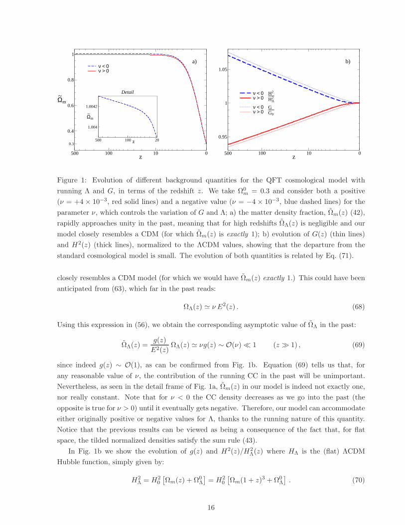
In Fig. 1, we show the evolution of different background quantities in this model in terms of

the redshift z. For the plots, we have used Ω0m = 0.3 and both a positive (ν = +4 × 10−3, red

solid line) and a negative value (ν = −4× 10−3, blue dashed line) for the parameter ν. As we will

see later in this section, according to LSS and nucleosynthesis considerations, we expect ν to be

(at most) of order 10−3, so these are reasonable values. In Fig. 1a, we plot the evolution of the

matter density fraction, Ωm(z) (42), which rapidly approaches unity in the past. This means that

ΩΛ(z) is negligible for high redshifts – recall the sum rule (43) – so that in this regime our model

15

010100500z

0.3

0.4

0.6

0.8

1

~Ωm

ν < 0ν > 0

20100500 z

1.004

1.0042

~Ωm

Detail

a)

010100500z

0.95

1

1.05

ν < 0ν > 0Nν < 0ν > 0

H2

H2Λ

GG0

b)

Figure 1: Evolution of different background quantities for the QFT cosmological model with

running Λ and G, in terms of the redshift z. We take Ω0m = 0.3 and consider both a positive

(ν = +4 × 10−3, red solid lines) and a negative value (ν = −4 × 10−3, blue dashed lines) for the

parameter ν, which controls the variation of G and Λ; a) the matter density fraction, Ωm(z) (42),

rapidly approaches unity in the past, meaning that for high redshifts ΩΛ(z) is negligible and our

model closely resembles a CDM (for which Ωm(z) is exactly 1); b) evolution of G(z) (thin lines)

and H2(z) (thick lines), normalized to the ΛCDM values, showing that the departure from the

standard cosmological model is small. The evolution of both quantities is related by Eq. (71).

closely resembles a CDM model (for which we would have Ωm(z) exactly 1.) This could have been

anticipated from (63), which far in the past reads:

ΩΛ(z) ≃ ν E2(z) . (68)

Using this expression in (56), we obtain the corresponding asymptotic value of ΩΛ in the past:

ΩΛ(z) =g(z)

E2(z)ΩΛ(z) ≃ νg(z) ∼ O(ν) ≪ 1 (z ≫ 1) , (69)

since indeed g(z) ∼ O(1), as can be confirmed from Fig. 1b. Equation (69) tells us that, for

any reasonable value of ν, the contribution of the running CC in the past will be unimportant.

Nevertheless, as seen in the detail frame of Fig. 1a, Ωm(z) in our model is indeed not exactly one,

nor really constant. Note that for ν < 0 the CC density decreases as we go into the past (the

opposite is true for ν > 0) until it eventually gets negative. Therefore, our model can accommodate

either originally positive or negative values for Λ, thanks to the running nature of this quantity.

Notice that the previous results can be viewed as being a consequence of the fact that, for flat

space, the tilded normalized densities satisfy the sum rule (43).

In Fig. 1b we show the evolution of g(z) and H2(z)/H2Λ(z) where HΛ is the (flat) ΛCDM

Hubble function, simply given by:

H2Λ = H2

0

[

Ωm(z) + Ω0Λ

]

= H20

[

Ωm(1 + z)3 +Ω0Λ

]

. (70)

16

Taking into account (61) and (67) we obtain, to order ν,

H2(z)

H2Λ

= g(z)Ωm(z) + ΩΛ(z)

Ωm(z) + Ω0Λ

≃ g(z)

(

1 + νΩm(z)− Ω0

m

Ωm(z) + Ω0Λ

)

. (71)

Therefore the evolutions of H2(z)/H2Λ and g(z) are expected to be very similar, as indeed shown in

Fig. 1b. Furthermore, both quantities stay close to 1, so the deviation from the standard ΛCDM

evolution is reasonably small, although it maybe large enough so as to be detected in a future

generation of precision cosmology experiments. For instance, for the values of ν and Ω0m that we

are considering, the relative deviations of ΩΛ(z), g(z) and H2(z) at z = 2 with respect to the

standard model values are (approximately) 4%, 1% and 0.5%, respectively.

5.1 Constraints from large-scale structure

Let us now move to the detailed study of the growth of matter density perturbations in our model,

and further elaborate on some important issues raised in section 3. The matter power spectrum

for a sufficiently recent value of the scale factor (a≫ aeq) can be written as:

P (k, a) ≡ |δm(k, a)|2 = AknT 2(k)D2(k, a) . (72)

Here A is a normalization coefficient; n is the scalar spectral index (which gives us the shape of

the primordial spectrum; e.g. n = 1 if we assume a Harrison-Zel’dovich spectrum); T (k) is the

transfer function, which does not depend on the initial conditions but only on the physics of the

microscopic constituents; i.e. it encodes the modifications of the primordial spectrum that arise

when taking into account the dynamical properties of the particles and their interactions. The

T (k) function receives non-trivial contributions only from the evolution of the different (comoving)

wavelenghts λ ∼ 1/k in the epochs of radiation, horizon crossing and radiation/matter equality,

i.e. it reflects the k-dependent features that occur at early times when a moves from a ≪ aeq to

a≫ aeq. In general, the form of T (k) depends on the cosmological model under consideration, and

determines to a large extent the final shape of the spectrum. However, for the late time evolution

(a≫ aeq), there might be more distortions of the spectrum in models that depart significantly from

the standard ΛCDM scenario (for which there are no further k-dependence beyond that already

encoded in the transfer function). These additional, model-dependent, effects are reflected in the

k-dependence of the growth factor D(k, a) in Eq. (72). A dependence of this sort would appear e.g.

in models of type ii) in section 2 where the CC decays into matter, as it was previously studied

in [28]. However, our claim (formulated in section 3) is that this is not the case for the variable

CC and G models under consideration, i.e. models of type iv) in section 2 with self-conservation

of matter, provided that G is a slowly varying function of time. Obviously this is so for the model

studied in the previous section, where G varies logarithmically with the expansion of the universe,

see Eq. (65). For these models, and of course also for the standard ΛCDM model, the growth factor

is independent of k and can be written as

D(a) =δm(a)

δCDM(a0), (73)

where δCDM(a0) is the present matter density contrast in a pure cold dark matter (CDM) scenario,

taken as a fiducial model.

17

5.1.1 More on the transfer function for variable ρΛ and G models.

A few additional comments on the transfer function are now in order. As previously commented,

we expect the transfer function in our model to be the same as for the ΛCDM. First of all, let us

try to better justify this expectation, which implies that the shape of the matter power spectrum

in our model coincides with that of a ΛCDM with the same value of Ω0m. Then we show that

we can still constrain our model by means of the growth factor, obtaining bounds in very good

agreement with those arising from primordial nucleosynthesis.

The scale dependence of the transfer function for CDM models is different for large scales (small

k’s), where T (k) = 1, and small scales, where it asymptotes to ln (k)/k2 [35]. The turnaround

occurs at the value k = keq, corresponding exactly to the scale that enters the Hubble horizon

(H−1) at the moment of matter-radiation equality, i.e. at the point a = aeq which satisfies

Ωm(aeq) = Ωr(aeq), hence

aeq =Ω0r

Ω0m

, (74)

where Ω0r ∼ 10−4 is the present density of radiation. The modes that enter the horizon at

the equality time, with comoving wavelength λeq, have a physical wavelength that follows upon

multiplication with the scale factor (74), i.e. λeq aeq = 1/H(aeq), or, equivalently,

keq = aeqH(aeq) . (75)

Obviously, since H decreases with time the perturbations with wavelenght shorter than λeq (i.e.

those with with k > keq) will enter the Hubble horizon before the matter-radiation equality, i.e. in

the radiation era (t < teq). From this moment until t = teq, the growth of inhomogeneities in the

cold DM component becomes suppressed because the expansion rate during the radiation epoch is

faster than the characteristic collapsing rate of the CDM. As a result, the modes in the radiation

epoch can grow at most logarithmically with the scale factor. Only after the cold component begins

to dominate (t > teq) the amplitude of the formerly inhibited modes starts growing linearly with

the scale factor. Finally, as light can only cross regions smaller than the horizon, the suppression in

the radiation epoch does not affect the large-scale perturbations (k ≪ keq), which enter the horizon

in the matter epoch. Such different behavior of the perturbations according to their entrance in

the horizon before or after the time of equality is the origin of the characteristic shape of the

transfer function for CDM-like models in the various available parameterizations [35].

From the previous standard discussion, it is apparent that the shape of the transfer function

depends critically on the value of keq, which in turn depends on aeq and H(aeq). In the models we

are studying, dark matter and radiation are separately conserved, and therefore the value of aeq

will not change with respect to the standard one, Eq. (74). So the remaining issue is to clarify if

the change of H(aeq) in our model as compared to the corresponding ΛCDM value is significant

or not. The answer follows easily from Eq. (71). At the high redshift where equality of matter and

radiation occurs, z = O(103) ≫ 1, the function that accompanies ν on the r.h.s. of that equation

is virtually equal to one, and we are left with

H(aeq) ≃√

g(aeq) (1 + ν)HΛ(aeq) . (76)

18

Here, as before, HΛ is just the standard ΛCDM Hubble rate. For the maximal values of ν that we

will be considering (|ν| ∼ O(10−3), see the subsequent sections), it is easy to see from (65) that

∣

∣

∣

∣

√

g(aeq)− 1

∣

∣

∣

∣

≃ |ν| ln H(aeq)

H0∼ 1% , (77)

where the expansion rate at the time of equality is H(aeq) ∼ 105H0. We see that the change of

H(aeq) with respect to HΛ(aeq) is mainly caused by the variation of g from 1 at t = teq. However,

numerically, the effect is very small. These results allow us to safely conclude that the value of keq

expected in our model is essentially the same as that of the ΛCDM model, up to differences of 1%

at most. Given that in the ΛCDM model the (comoving) wavenumber at equality is

keq = aeqHΛ(aeq) =

√

2

Ω0R

Ω0mH0 ∼ 10−2 hMpc−1 , (78)

we see from this expression that a 1% change in√

g(aeq) – hence in H(aeq) – is equivalent to a 1%

change in Ω0m in the standard scenario (i.e. with g = 1). This variation is too small to be within

reach of the present observations (see the next section), and can be safely neglected.

The final point is that, as argued throughout this section, neither ρΛ nor its perturbations or

those of G are important in the past. Therefore, the evolution of the perturbations both in the

radiation and in the matter-dominated eras (and both in the case of sub-Hubble and super-Hubble

perturbations) remains essentially unchanged.

All in all, we expect that the transfer function in the model under consideration is very close

to that of a ΛCDM with the same value of Ω0m. From the line of our argumentation that we have

used, it is not difficulty to convince oneself that this result can be extended to any model with

variable Λ and G, and self-conserved matter, as long as G(a) is not changing too fast. Adding

this property to the fact – cf. section 3 – that the late growth of matter density perturbations in

these models does not depend on the wavenumber, the final robust conclusion is that the matter

power spectrum for models within the scenario iv) of section 2 will present the same shape as

in the standard ΛCDM case. Therefore, the spectrum shape will not be useful to constrain the

additional free parameters of the model. This is in sharp contrast to models within scenario ii),

in which there is an exchange between dark matter and vacuum energy. For these models there

is an explicit dependence on k beyond that of the transfer function and this produces a late time

distortion of the power spectrum with respect to the ΛCDM. As indicated, this was exemplified

in Ref. [28, 29] for the case of an evolution law of the type (53).

To summarize, there is a significant difference between the running QFT vacuum model (53)

when studied either in scenario ii) or when considered in scenario iv). While in Ref. [28, 29] the

shape of the spectrum was used to restrict the parameter ν for type ii) models, in the next section

we show that for the alternative type iv) models, being them shape-invariant with respect to the

ΛCDM model, one can make use of the amplitude of the power spectrum in order to constrain the

free parameters.

19

5.1.2 The spectrum amplitude as a way to constrain running G and Λ models.

The normalization of the matter power spectrum on scales relevant to large-scale structure can

be performed through different methods [46], e.g. from the microwave-background anisotropies or

by measuring the local variance of galaxy counts within certain volumes. One of the most robust

ways to do it is through the number density of rich galaxy clusters [44,45], which is very sensitive

to the amplitude of the dark matter fluctuations that collapsed to form them. The typical scales

for these fluctuations are of order 10 Mpc, which are the smallest ones still in the linear part of

the spectrum. The cluster method determines the amplitude of the power spectrum on just that

length scale (corresponding to wavenumbers in the upper end of those explored with this method).

The normalization is usually phrased in terms of σ8, the root mean square mass fluctuation in

spheres with radius 8h−1 Mpc (i.e. ∼ 10 Mpc, for h ≃ 0.7). By assuming a ΛCDM model, these

studies are able to provide constraints in the σ8 - Ω0m plane. An important feature is that the

results are approximately independent of the spectrum shape and galaxy bias [44]. For instance,

in this last reference, it is found the relation:

σ8 =(

0.495+0.034−0.037

)

(Ω0m)−0.60 , (79)

valid for spatially flat models with a wide range of shapes (in particular, valid for 0.2 ≤ Ω0m ≤ 0.8).

When combined with CMB analyses, cluster studies can determine both σ8 and Ω0m. In a recent

work [45], local cluster counts are used in conjunction with WMAP5 data to find:

Ω0m = 0.30+0.03

−0.02 (68%) . (80)

We will use this result to constrain our G-variable model. In order to do this, we first define the

“amount of growth”, namely the square of the growth factor (73) at present, D2(a0), which appears

directly in the formula of the power spectrum, Eq. (72). The idea is to compare the amount of

growth in our model model with the amount of growth in the ΛCDM model with Ω0m = 0.30.

From the standard expression for the growth factor in the ΛCDM model [35] one finds that a

∼ 10% variation in Ω0m given by (80) represents a ∼ 5% change in the amount of growth. As the

determination (80) entails only a 1σ constraint, we will be conservative and allow up to a 10%

deviation in the amount of growth of our model with respect to the ΛCDM model. We are thus

asking our model to pass the following “F-test” [29,47]:

F =

∣

∣

∣

∣

1− D2(a0,Ω0m, ν)

D2(a0, 0.3, 0)

∣

∣

∣

∣

≤ 0.1 . (81)

Notice that D2(a0, 0.3, 0) in the denominator is just the amount of growth in the ΛCDM for the

central value of (80), whereas in the numerator we have the amount of growth for the model under

consideration at a given non-vanishing value of the relevant parameter ν, with Ω0m left as a free

parameter. As a result, the constraint (81) will generate contours in the ν - Ω0m plane which will

define the allowed region in parameter space.

The admissible values for Ω0m should, in principle, be those compatible with the shape of the

spectrum. However, the shape has been measured by the 2dFGRS and SDSS surveys, existing

20

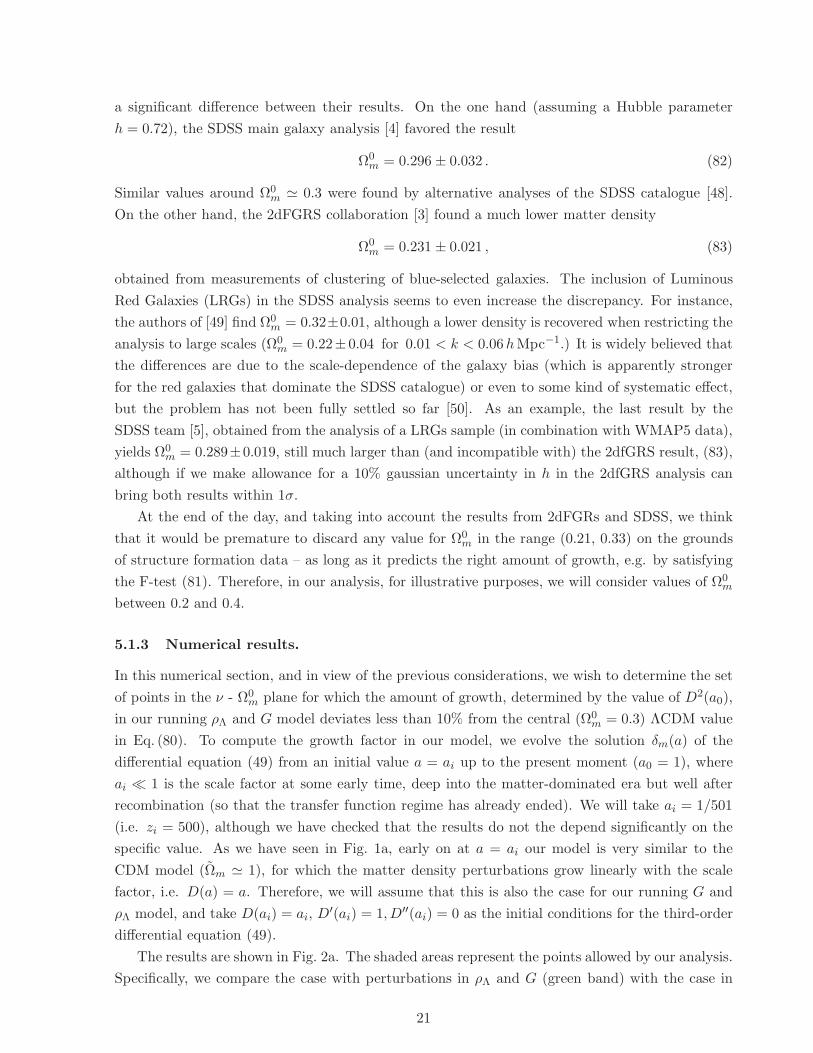
a significant difference between their results. On the one hand (assuming a Hubble parameter

h = 0.72), the SDSS main galaxy analysis [4] favored the result

Ω0m = 0.296 ± 0.032 . (82)

Similar values around Ω0m ≃ 0.3 were found by alternative analyses of the SDSS catalogue [48].

On the other hand, the 2dFGRS collaboration [3] found a much lower matter density

Ω0m = 0.231 ± 0.021 , (83)

obtained from measurements of clustering of blue-selected galaxies. The inclusion of Luminous

Red Galaxies (LRGs) in the SDSS analysis seems to even increase the discrepancy. For instance,

the authors of [49] find Ω0m = 0.32±0.01, although a lower density is recovered when restricting the

analysis to large scales (Ω0m = 0.22± 0.04 for 0.01 < k < 0.06hMpc−1.) It is widely believed that

the differences are due to the scale-dependence of the galaxy bias (which is apparently stronger

for the red galaxies that dominate the SDSS catalogue) or even to some kind of systematic effect,

but the problem has not been fully settled so far [50]. As an example, the last result by the

SDSS team [5], obtained from the analysis of a LRGs sample (in combination with WMAP5 data),

yields Ω0m = 0.289±0.019, still much larger than (and incompatible with) the 2dfGRS result, (83),

although if we make allowance for a 10% gaussian uncertainty in h in the 2dfGRS analysis can

bring both results within 1σ.

At the end of the day, and taking into account the results from 2dFGRs and SDSS, we think

that it would be premature to discard any value for Ω0m in the range (0.21, 0.33) on the grounds

of structure formation data – as long as it predicts the right amount of growth, e.g. by satisfying

the F-test (81). Therefore, in our analysis, for illustrative purposes, we will consider values of Ω0m

between 0.2 and 0.4.

5.1.3 Numerical results.

In this numerical section, and in view of the previous considerations, we wish to determine the set

of points in the ν - Ω0m plane for which the amount of growth, determined by the value of D2(a0),

in our running ρΛ and G model deviates less than 10% from the central (Ω0m = 0.3) ΛCDM value

in Eq. (80). To compute the growth factor in our model, we evolve the solution δm(a) of the

differential equation (49) from an initial value a = ai up to the present moment (a0 = 1), where

ai ≪ 1 is the scale factor at some early time, deep into the matter-dominated era but well after

recombination (so that the transfer function regime has already ended). We will take ai = 1/501

(i.e. zi = 500), although we have checked that the results do not the depend significantly on the

specific value. As we have seen in Fig. 1a, early on at a = ai our model is very similar to the

CDM model (Ωm ≃ 1), for which the matter density perturbations grow linearly with the scale

factor, i.e. D(a) = a. Therefore, we will assume that this is also the case for our running G and

ρΛ model, and take D(ai) = ai, D′(ai) = 1,D′′(ai) = 0 as the initial conditions for the third-order

differential equation (49).

The results are shown in Fig. 2a. The shaded areas represent the points allowed by our analysis.

Specifically, we compare the case with perturbations in ρΛ and G (green band) with the case in

21

-0.01 0 0.01 0.02ν

0.2

0.25

0.3

0.35

0.4

Ωm0

a)

δG = 0

δG = 0

-0.01 0 0.01 0.02ν

0.2

0.25

0.3

0.35

0.4

Ωm0

b)

Scenario ii)

Scenario iv)

δG = 0

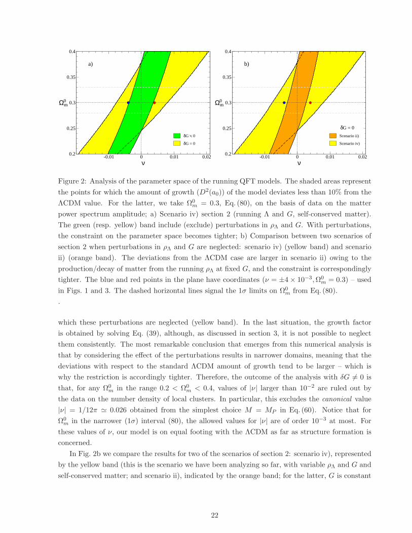
Figure 2: Analysis of the parameter space of the running QFT models. The shaded areas represent

the points for which the amount of growth (D2(a0)) of the model deviates less than 10% from the

ΛCDM value. For the latter, we take Ω0m = 0.3, Eq. (80), on the basis of data on the matter

power spectrum amplitude; a) Scenario iv) section 2 (running Λ and G, self-conserved matter).

The green (resp. yellow) band include (exclude) perturbations in ρΛ and G. With perturbations,

the constraint on the parameter space becomes tighter; b) Comparison between two scenarios of

section 2 when perturbations in ρΛ and G are neglected: scenario iv) (yellow band) and scenario

ii) (orange band). The deviations from the ΛCDM case are larger in scenario ii) owing to the

production/decay of matter from the running ρΛ at fixed G, and the constraint is correspondingly

tighter. The blue and red points in the plane have coordinates (ν = ±4× 10−3,Ω0m = 0.3) – used

in Figs. 1 and 3. The dashed horizontal lines signal the 1σ limits on Ω0m from Eq. (80).

.

which these perturbations are neglected (yellow band). In the last situation, the growth factor

is obtained by solving Eq. (39), although, as discussed in section 3, it is not possible to neglect

them consistently. The most remarkable conclusion that emerges from this numerical analysis is

that by considering the effect of the perturbations results in narrower domains, meaning that the

deviations with respect to the standard ΛCDM amount of growth tend to be larger – which is

why the restriction is accordingly tighter. Therefore, the outcome of the analysis with δG 6= 0 is

that, for any Ω0m in the range 0.2 < Ω0

m < 0.4, values of |ν| larger than 10−2 are ruled out by

the data on the number density of local clusters. In particular, this excludes the canonical value

|ν| = 1/12π ≃ 0.026 obtained from the simplest choice M = MP in Eq. (60). Notice that for

Ω0m in the narrower (1σ) interval (80), the allowed values for |ν| are of order 10−3 at most. For

these values of ν, our model is on equal footing with the ΛCDM as far as structure formation is

concerned.

In Fig. 2b we compare the results for two of the scenarios of section 2: scenario iv), represented

by the yellow band (this is the scenario we have been analyzing so far, with variable ρΛ and G and

self-conserved matter; and scenario ii), indicated by the orange band; for the latter, G is constant

22

and the CC exchanges energy with matter. In both cases, we are neglecting the perturbations5 in

ρΛ, which in scenario iv) implies that δG = 0 as well, cf. Eq. (36). The effective equation for the

matter density contrast in scenario ii) is the following:

δm +

(

2H +Ψ

ρm

)

δm −[

4πGρm − 2HΨ

ρm− d

dt

(

Ψ

ρm

)]

δm = 0 , (84)

Ψ ≡ ρm + 3Hρm = −ρΛ . (85)

This equation, whose primary derivation was performed within the Newtonian formalism [51],

can also can be derived from the general relativistic treatment of perturbations [21], as explained

in [18]. It is convenient to express it in terms of the scale factor a:

δ′′m +

(

3

a+H ′

H+

Ψ

ρmHa

)

δ′m −[

3

2Ωm − 2

H

Ψ

ρm− a

H

(

Ψ

ρm

)

′]

δma2

= 0 . (86)

For Ψ = 0, we recover equation (39) (with δG = 0), as expected. In Fig. 2b, we see that the

differences in the amount of growth with respect to the ΛCDM case are larger for scenario ii); the

natural interpretation is that this is caused by the production/decay of matter associated to the

time evolution of ρΛ.

The blue and red points in Figs. 2a,b correspond to the values analyzed in Fig. 1, i.e. Ω0m = 0.3

and ν = ±4× 10−3. We will use again these values to exemplify the evolution of the matter and

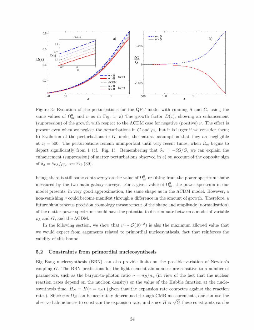
Newton’s coupling perturbations. Fig. 3a shows the growth factor as a function of the redshift,

both when allowing for perturbations in G and ρΛ and when they are neglected. For ν < 0, our

model predicts more growth than the ΛCDM model. When δG = 0, this is just due to the fact that

ρΛ is decreasing when we go into the past, so its repulsive effect diminishes. When considering the

perturbations in G and Λ, the deviation with respect to the standard case increases even more,

as already commented in Fig. 2a. The opposite situation occurs for ν > 0; here the suppression

of growth is attributed to the enhanced repulsion of matter associated to a positive ρΛ, which

is increasing with z. Such suppression is larger when we include the G and Λ perturbations. A

detailed study of these effects for model ii) of section 2 was performed in Ref. [29], in an effective

approach with no perturbations in the CC.

In Fig. 3b, the evolution of δG/G, as obtained from Eq. (37), is depicted. This equation only

determines δG′, so we need to give an initial condition for δG at a = ai. In order to do so, we note

that the fact that Ωm(z) ≃ 1 in the past (reflected in Fig. 1a) ensures that the perturbations in G

are not playing any important role, according to our discussion at the end of section 3. Therefore,

the most natural condition seems to be δG(ai) = 0, and, besides, we expect δG/G to remain

negligible until very recent times (z . 10), when Ωm begins to depart from 1. This is indeed what

can be seen in Fig. 3b, giving additional support to our assumption. Let us remind from (36) that

δΛ = −δG/G. Thus, for ν < 0 we have δG > 0 and hence δΛ < 0, which explains the further

enhancement in the growth of matter perturbations with respect to the case with δG = δρΛ = 0.

The main conclusion of this section is that for ν of order 10−3 or smaller, our model is in

perfect agreement with recent data on the normalization of the power spectrum. For the time

5Remember that within scenario ii), including the perturbations in Λ causes the growth factor to become scale-

dependent [28], D = D(k, a), so the kind of analysis we are performing here would be no longer possible.

23

010 120z

0.2

0.4

0.6

0.8

D(z)

ν < 0ν > 0.ΛCDM.ν < 0ν > 0

0.10.2 0z

0.7

0.75

0.8

D(z)

Detail

δG = 0

δG = 0

a)

010100500z

-0.005

0

0.005

δGG

ν < 0ν > 0 b)

Figure 3: Evolution of the perturbations for the QFT model with running Λ and G, using the

same values of Ω0m and ν as in Fig. 1; a) The growth factor D(z), showing an enhancement

(suppression) of the growth with respect to the ΛCDM case for negative (positive) ν. The effect is

present even when we neglect the perturbations in G and ρΛ, but it is larger if we consider them;

b) Evolution of the perturbations in G, under the natural assumption that they are negligible

at zi = 500. The perturbations remain unimportant until very recent times, when Ωm begins to

depart significantly from 1 (cf. Fig. 1). Remembering that δΛ = −δG/G, we can explain the

enhancement (suppression) of matter perturbations observed in a) on account of the opposite sign

of δΛ = δρΛ/ρΛ, see Eq. (39).

being, there is still some controversy on the value of Ω0m resulting from the power spectrum shape

measured by the two main galaxy surveys. For a given value of Ω0m, the power spectrum in our

model presents, in very good approximation, the same shape as in the ΛCDM model. However, a

non-vanishing ν could become manifest through a difference in the amount of growth. Therefore, a

future simultaneous precision cosmology measurement of the shape and amplitude (normalization)

of the matter power spectrum should have the potential to discriminate between a model of variable

ρΛ and G, and the ΛCDM.

In the following section, we show that ν ∼ O(10−3) is also the maximum allowed value that

we would expect from arguments related to primordial nucleosynthesis, fact that reinforces the

validity of this bound.

5.2 Constraints from primordial nucleosynthesis

Big Bang nucleosynthesis (BBN) can also provide limits on the possible variation of Newton’s

coupling G. The BBN predictions for the light element abundances are sensitive to a number of

parameters, such as the baryon-to-photon ratio η = nB/nγ (in view of the fact that the nuclear

reaction rates depend on the nucleon density) or the value of the Hubble function at the nucle-

osynthesis time, HN ≡ H(z = zN ) (given that the expansion rate competes against the reaction

rates). Since η ∝ ΩB can be accurately determined through CMB measurements, one can use the

observed abundances to constrain the expansion rate, and since H ∝√G these constraints can be

24

directly translated6 into bounds on gN ≡ g(zN ), where g(z) was defined in Eq. (57).

The current constraints on gN available in the literature usually make use either of the deu-

terium abundance (D/H) or the 4He mass fraction (Yp). Deuterium has the advantage that it is

not produced in significant quantities after nucleosynthesis; its primordial abundance can be deter-

mined in a quite precise manner by studying the spectrum of the light from distant quasars, which

exhibits an absorption line corresponding to the deuterium present in (high-redshift) intervening

neutral hydrogen systems. This turns deuterium into an excellent probe of the universe at the

time of BBN. However, its predicted abundance depends much more strongly on η than on HN .

As a consequence, the constraints on gN based on deuterium measurements are not very stringent.

For instance, in [52] it is found gN = 1.01+0.20−0.16 at the 68.3% confidence level or:

gN = 1.01+0.42−0.30 (95%) . (87)

The abundance of 4He is much more sensitive to the expansion rate, but accurate observational

values are difficult to obtain, since there are many potential sources of systematic uncertainties [53].

As a result, a wide range of values for Yp can be found in the literature, see e.g. Table 12 in [54]. In

this reference, the authors used Yp = 0.250±0.003 (in fact, they use Yp in combination with D/H,

although the dominant effect is that of helium [54]) to obtain (see section 8.2.5 of the latter):

0.964 < gN < 1.086 (95%) , (88)

whereas in [55] a more conservative range for the 4He mass fraction is adopted (Yp = 0.2495 ±0.0092), leading to:

0.9 < gN < 1.13 (68%) . (89)

Applying (87)-(89) to our model, we can effectively constrain our parameter ν. In order to do so,

we compute gN from (65):

gN =1

1 + ν ln(

H2N/H

20

) ≃ 1

1 + ν ln [Ω0r(1 + zN )4]

, (90)

where Ω0r is the radiation energy density fraction at present, we have neglected both the matter

and CC contributions to the expansion rate at z = zN , and is evident that gN can be neglected as

well in the logarithm. Taking Ω0r ∼ 10−4 (which includes photons and three light neutrino species)

together with zN ∼ 109, and comparing the last expression to (87)-(89), we find:

From (87) −→ −4.1× 10−3 . ν . 5.5× 10−3

From (88) −→ −1.1× 10−3 . ν . 5.1× 10−4

From (89) −→ −1.6× 10−3 . ν . 1.5× 10−3

Let us remind that (88) was derived from a value for Yp with a (possibly unrealistic) very small

error and that (89) is a 68% value (whereas the other two limits are given at the 95% confidence

level.) In any case, the conclusion arising from this nucleosynthesis analysis seems to be that the

6Provided that the total energy density at z = zN is approximately the same as in the standard case. Eq. (69)

shows that this condition is satisfied in our model.

25

parameter ν can be, at most, of order 10−3. This is in complete agreement with the constraint on ν

obtained in section 5.1 from structure formation considerations. Therefore, we have arrived to the

same result by using two very different methods, which gives additional credit to our conclusions.

6 Conclusions

In this paper, we have derived the general set of cosmological perturbation equations for FLRW

models with variable cosmological parameters ρΛ and G in which matter is covariantly conserved.

To our knowledge, this is the first time that a complete set of coupled differential equations for δρΛ

and δG is presented in the literature. We have shown that the linear growth of matter perturbations

of this model, D(a) ∝ δm(a), is independent of the wave number k. Adding this property to the

fact that we generally expect these models to present the same transfer function as the ΛCDM,

the scaling dependence and hence the shape of the power spectrum will not change with the late

time evolution and it will coincide with that of the ΛCDM model. This fact is remarkable as it is

in contrast to the situation, more frequently studied in the literature, in which the time-evolving

vacuum models exchange energy with matter at fixed Newton’s coupling G [18].

We have exemplified the difference in the power spectrum of running vacuum models, with and

without matter conservation, by considering the class of cosmological models characterized by the

running CC law (53), which we call quantum field vacuum models because the evolution of the

CC in them is of the form that one would naturally expect from QFT, and more specifically from

the renormalization group evolution of the cosmological parameters. Such quantum field vacuum

models depend on a single parameter ν, which acts as the β-function for the running of the vacuum

energy density ρΛ = ρΛ(H) and the running gravitational coupling G = G(H). It is interesting to

note that while the running of the vacuum energy ρΛ(H) is quadratical in the expansion rate, the

running of G(H) is logarithmic in H, Eq. (65), and therefore much milder. For ν > 0, the running

of G is asymptotically free, hence G decreases (resp. increases) logarithmically with the redshift

(resp. with the expansion), whereas for ν < 0 it decreases with the expansion. The background

evolution of these models was studied in [24,25].

In the present paper, we have concentrated on the study of the cosmic perturbation equations

of the running ρΛ(H) and G(H) models. After confronting the predicted matter growth with the

various cosmological data, we have found that the final region of the parameter space is a natu-

ralness region in which ν could be, in absolute value, of order 10−3 at most. We have also checked

that this bound is compatible with the restriction on G variation that follows from primordial

nucleosynthesis. Remarkably enough, the results emerging from the perturbations analysis are

derived from the amplitude of the power spectrum rather than from its shape. Numerically, the

obtained upper bound on ν is perfectly compatible with the quantum field theoretical definition

of this parameter, see Eq. (60), and it implies that the mass scales that would enter the quantum

running of the cosmological parameters could be one order of magnitude below the Planck scale, at

most. The result |ν| < O(10−3) is also compatible with previous analyses, using various indepen-

dent procedures, of models with running ρΛ in which the vacuum can decay into matter [18,28–30].

This decay feature, however, is impossible for the models with running ρΛ(H) and G(H) that we

26

have studied here, and this is the basic reason why they can exhibit the same power spectrum

profile as the ΛCDM. We cannot exclude that this property could have been responsible for the

fact that we have observationally missed this fundamental possibility up to now. As we have

emphasized, we expect that these models should eventually be testable in the next generation of

precision cosmology observations from the analysis of the spectrum amplitude, rather than of the

spectral shape.

Acknowledgments. JG and JS have been supported in part by MEC and FEDER under

project FPA2007-66665, by the Spanish Consolider-Ingenio 2010 program CPAN CSD2007-00042

and by DIUE/CUR Generalitat de Catalunya under project 2009SGR502. JF thanks CNPq and

FAPES, and ISh is grateful to CNPq, FAPEMIG, FAPES and ICTP for the partial support.

7 Appendix: cosmic perturbations in the Newtonian gauge

In this appendix, we sketch the derivation of the perturbation equations in the Newtonian or

longitudinal gauge [56]. Our aim is to explicitly check that the same physical consequences that

we have derived in section 3 for the synchronous gauge are recovered in another gauge. In this

way, we confirm in our particular context the general expectation that calculations of cosmic

perturbations at deep sub-horizon scales should not present significant gauge dependence.

The most general perturbation of the spatially flat FLRW metric can be conveniently written

as follows [56]

ds2 = a2(η)[(1 + 2ψ)dη2 − ωi dη dxi − ((1− 2φ)δij + χij) dx

idxj ] , (91)

where η is the conformal time, defined through dη = dt/a. The above metric is expressed in the

notation of [21] and consists of the 10 degrees of freedom associated to the two scalar functions ψ, φ,

the three components of the vector function ωi (i = 1, 2, 3), and the five components of the traceless

second-rank tensor χij. Clearly, the synchronous gauge that we used in section 3 is obtained by

setting ψ = 0, ωi = 0 and absorbing the function φ into the trace of χij , which then contributes

six degrees of freedom. In this gauge, the metric part of the analysis of cosmic perturbations is

tracked by the nonvanishing trace of the metric disturbance: h ≡ gµν hµν = gij hij = −hii/a2.The corresponding equations have been presented in detail in section 3 after defining the “hat

variable”: h = −∂h/∂t = ∂(

hii/a2)

/∂t.

An alternative possibility is to use the (conformal) Newtonian gauge [56,57]. In this case, we

set ωi = χij = 0 (∀i, j) in Eq. (91). A useful feature of this gauge is that the metric is diagonal

and another is that, in the Newtonian limit, ψ plays the role of the gravitational potential. It is

now straightforward to repeat the calculation of the perturbation equations in a similar way as in

section 3. In the absence of anisotropic shear stress (which is always the case with non-relativistic

particles, such as baryons and dark matter), the perturbed Einstein’s equations for i 6= j give

ψ = φ [57], see also [58]. Indicating by a prime the derivatives with respect to the scale factor

27

(f ′ ≡ df/da), the final perturbation equations in that gauge read as follows:

k2φ = −4πa2

G

[

δρm + δρΛ + 3Hρma2

k2θ

]

+ (ρm + ρΛ)δG

,

δρ′m + ρm

(

θ

aH− 3φ′

)

+3

aδρm = 0 ,

θ′ +2

aθ =

k2

Ha3φ , (92)

δG′(ρm + ρΛ) + δGρ′Λ +G′(δρm + δρΛ) +Gδρ′Λ = 0 ,

GδρΛ + ρΛδG +

(

Ha3

k2

)

ρmG′θ = 0 .

Notice that the role of h in the synchronous gauge is taken up here by the variable φ = ψ, which

turns out to satisfy an algebraic rather than a differential equation. Worth noticing is also the fact

that the last two equations of (92) are identical to equations (32) and (33) respectively, except that

in the present case we used derivatives with respect to the scale factor rather than with respect to

the cosmic time (as in this way length scales can be better compared with the horizon).

We are now ready to show that for deep sub-Hubble (sub-horizon) perturbations, i.e. those

satisfying k/(aH) ≫ 1, these equations lead to the same second and third-order differential equa-

tions for the normalized matter overdensity δm = δρm/ρm, which we have previously found within

the synchronous gauge in section 3. To start with, the first equation of (92) can be cast as:

φ = −3

2

H2a2

k2

Ωm δm + ΩΛ δΛ +δG

G

, (93)

where δΛ = δρΛ/ρΛ, and of course we use the same notation as in section 3 concerning the

parameters Ωm and ΩΛ. In the previous equation, we have dropped the term 3Hρm a2 θ/k2 since it

is negligible for sub-Hubble perturbations. In this same regime of perturbations, Eq.(93) obviously

implies that φ≪ δm. Next, let us note that the second equation of (92) can be simplified by using

the conservation of matter, giving:

δ′m +θ

aH= 3φ′ . (94)

Differentiating this equation and using the third one in (92) to substitute for θ′, we find:

δ′′m − θ

aH

(

3

a+H ′

H

)

= 3φ′′ −(

k

Ha

)2 φ

a2. (95)

Furthermore, if we eliminate θ from this equation by means of (94) and also φ using (93), we get:

δ′′m − 3φ′′ + (δ′m − 3φ′)

(

3

a+H ′

H

)

=3

2a2

Ωmδm + ΩΛδΛ +δG

G

. (96)

Again we can neglect the terms that are small at sub-Hubble scales; for example, in the previous

equation we can neglect φ′ (φ′′) as compared to δ′m (δ′′m) on account of the previously discussed

relation φ≪ δm. In this way, we arrive at:

δ′′m +

(

3

a+H ′

H

)

δ′m =3

2a2

Ωmδm + ΩΛδΛ +δG

G

. (97)

28

The almost final step is to substitute δΛ by means of the last equation of (92). Once more, we

can argue (as we did in section 3) that apart from the damping factor Ha/k ≪ 1 for the sub-

Hubble modes, there are additional suppression effects, such as the presence of G′ which is small

as compared to G, and hence (G′/G)θ can be considered almost second-order. Therefore, the last

equation of (92) boils down in practice to GδρΛ + ρΛδG = 0, which simply renders δΛ = −δG/G.Using also the sum rule (43), the relation (97) finally takes on the simpler form

δ′′m +

(

3

a+H ′

H

)

δ′m =3Ωm

2a2

(

δm +δG

G

)

. (98)

This equation exactly coincides with Eq.(39), showing indeed that our result was not gauge-

dependent. Obtaining the third-order equation for δm is now straightforward. From the last two

equations of (92) one can show that

δm = −(δG)′

G′. (99)

From here we proceed as in section 3 for the synchronous gauge, i.e. we differentiate Eq.(98)

with respect to the scale factor and we reach once more the third order differential equation (49).

(q.e.d.)

Some discussion is now in order. Let us first note that the variable cosmological constant

scenario ii) of section 2, whose perturbation equations were originally analyzed in [28] in the

synchronous gauge, has been reanalyzed in the Newtonian gauge in [32] and the same conclusions

have been attained. We should also mention a very recent paper [59] where a nice discussion is

made on comparing the synchronous and Newtonian gauges in the context of a model with self-

conserved DE and without DE perturbations. As it is well-known, in that case the two gauges

give the same evolution for the cosmological perturbations for scales well below the horizon – see

also [57, 60]. This feature was expected in our model too, even if it is a bit more complicated

than the one considered in [59] (our DE is also self-conserved, but we do have both DE and G

perturbations), and in fact the physical discussion about the gauge differences is very similar. In

the same reference, it is also pointed out that the k-dependent effects are negligible for large values

of k, although they could start to be appreciable for k < 0.01h (or, equivalently, for length scales

larger than ℓ ∼ 1/k ≃ 100h−1 Mpc.).

The issues about gauge dependence are of course important in general, because scale-dependent

effects may change from gauge to gauge. For instance, let us note that there is no counterpart

(within the synchronous gauge analysis considered in section 3) of the scale-dependent effects

introduced by the first equation (92). At the same time, there may be scale dependent features

which are tied to the particular cosmological model under consideration, and they need not show

up in another model, even if we compare them within the same gauge. Indeed, take once more the

model discussed in Ref. [59], where the DE is self-conserved and there are no perturbations in this

variable. In such situation, the cosmological perturbations of matter in the synchronous gauge turn

out to be exactly scale-independent (without any approximation). In our case, in contrast, there is

some residual scale dependence in the synchronous gauge, although it can be shown to be negligible

– as we have extensively discussed in section 3. Gauge differences, however, can be significant in

certain cases, specially for calculations involving very large scales, showing that in general it is

29

non-trivial to relate the perturbation variables to observable quantities in different gauges [57,60].

In that case, one must keep the appropriate k-dependence (as e.g. in the Newtonian gauge [59])

or resort to a gauge-invariant formalism [61, 62]. However, for the range of wavenumbers usually

explored in the analysis of the matter power spectrum (viz. 0.01h Mpc−1 < k < 0.2h Mpc−1 [3]),

the gauge differences, and in particular the k-dependence, should be small enough so as to be

licitly neglected. In other words, for such scales, the sub-Hubble approximation that we have

taken in this Appendix holds good and the calculations in the two gauges are found to be exactly

coincident, as we expected.

Finally, let us note that the reason why the physical discussion can be more transparent in

the Newtonian gauge is because the time slicing in this gauge respects the isotropic expansion

of the background. The synchronous gauge, instead, corresponds to free falling observers at all

points, entailing that its predictions are relevant only to length scales significantly smaller than

the horizon, but at these scales it renders the same physics as the Newtonian gauge [57,59,60].

References

[1] S. Weinberg, Rev. Mod. Phys., 61, 1, (1989).

[2] P. J. Peebles and B. Ratra, Rev. Mod. Phys., 75, 559, (2003); T. Padmanabhan, Phys. Rept.,

380, 235, (2003); E.J. Copeland, M. Sami and S. Tsujikawa, Int. J. of Mod. Phys. 15, 1753,

(2006); R. R. Caldwell and M. Kamionkowski, arXiv:0903.0866 [astro-ph.CO]; J. Frieman,

M. Turner and D. Huterer, Ann. Rev. Astron. Astrophys. 46, 385 (2008)

[3] S. Cole et al. [The 2dFGRS Collaboration], Mon. Not. Roy. Astron. Soc. 362 (2005) 505

[4] M. Tegmark, et al., Astrophys. J., 606, 702, (2004)

[5] B. A. Reid et al., arXiv:0907.1659 [astro-ph.CO]; W. J. Percival et al., arXiv:0907.1660 [astro-

ph.CO].

[6] A. G. Riess et al. [Supernova Search Team Collaboration], Astrophys. J. 607, 665 (2004); M.

Kowalski, et al., Astrophys. J., 686, 749, (2008); M. Hicken et al., arXiv:0901.4804; T.M.

Davis et al., Astrophys. J., 666, 716, (2007).

[7] D.N. Spergel, et al., Astrophys. J. Suplem., 170, 377, (2007); E. Komatsu, et al., Astrophys.

J. Suplem., 180, 330, (2009).

[8] I. L. Shapiro and J. Sola, Phys. Lett. B., 475 (2000) 236, hep-ph/9910462.

[9] A.D. Dolgov, in: The very Early Universe, Ed. G. Gibbons, S.W. Hawking, S.T. Tiklos

(Cambridge U., 1982); L.H. Ford, Phys. Rev. D35 (1987) 2339; R.D. Peccei, J. Sola and

C. Wetterich, Phys. Lett. B195 (1987) 183; J. Sola, Phys. Lett. B 228 (1989) 317.

[10] C. Wetterich, Nucl. Phys. B302 (1988) 668; P.J.E. Peebles and B. Ratra, Astrophys. J. 325

(1988) L17; B. Ratra and P.J.E. Peebles, Phys. Rev. D37 (1988) 3406; K. Coble, S. Dodelson,

30

J A. Frieman, Phys. Rev. D55 (1997) 1851; P.G. Ferreira and M. Joyce, Phys. Rev. D58

(1998) 023503; R.R. Caldwell, R. Dave and P.J. Steinhardt, Phys. Rev. Lett. 80 (1998) 1582;

P.J. Steinhardt, L.M. Wang and I. Zlatev, Phys. Rev. D59 (1999) 123504; V. Sahni and

L.M. Wang, Phys. Rev. D62 (2000) 103517.

[11] H. K. Jassal, J.S. Bagla, T. Padmanabhan, Phys.Rev. D72 103503, (2005); H.K. Jassal, J.S.

Bagla, T. Padmanabhan, Mon. Not. Roy. Astron. Soc. Letters 356, L11-L16, (2005).

[12] L. Samushia, B. Ratra, Astrophys. J. 650, L5, (2006); Astrophys. J. 680, L1, (2008).

[13] J.Q. Xia, H. Li, G.B. Zhao and X. Zhang, Phys. Rev. D78, 083524, (2008); G.B. Zhao, J.Q.

Xia, B. Feng, X. Zhang, Int. J. Mod.Phys. D16 1229, (2007); J.Q. Xia, G. B. Zhao, B. Feng,

H. Li, X. Zhang, Phys. Rev. D73 063521, (2006).

[14] J. Simon, L. Verde, R. Jimenez, Phys. Rev. D71 (2005) 123001.

[15] I.L. Shapiro, J. Sola, JHEP 02 (2002) 006, hep-th/0012227.

[16] I. L. Shapiro, J. Sola, Phys. Lett. B682 (2009) 105, arXiv:0910.4925 [hep-th]; see also the

review arXiv:0808.0315 [hep-th] on the QFT of the CC, and references therein.

[17] I. L. Shapiro, J. Sola, J. Phys. A40(2007) 6583, gr-qc/0611055, and references therein.

[18] S. Basilakos, M. Plionis and J. Sola, Phys. Rev. D80 (2009) 083511, arXiv:0907.4555.

[19] I.L. Shapiro, J. Sola, C. Espana-Bonet, P. Ruiz-Lapuente, Phys. Lett. 574B (2003) 149; JCAP

0402 (2004) 006; I.L. Shapiro, J. Sola, Nucl. Phys. Proc. Suppl. 127 (2004) 71; JHEP proc.

AHEP2003/013, astro-ph/0401015.

[20] J. Grande, J. Sola and H. Stefancic, JCAP 082006 011, gr-qc/0604057; Phys. Lett.

B645(2007)236, gr-qc/0609083; J. Phys. A40 (2007) 6787, gr-qc/0701090.

[21] J. Grande, A. Pelinson, J. Sola, Phys. Rev. D79 (2009) 043006, arXiv:0809.3462 [astro-ph];

arXiv:0904.3293 [astro-ph].

[22] F. Bauer, J. Sola, H. Stefancic, Phys. Lett. B 678 (2009) 427, arXiv:0902.2215;

arXiv:0912.0677; F. Bauer, Class. Quant. Grav. 27 (2010) 055001, arXiv:0909.2237 [gr-qc].

[23] O. Bertolami, Nuovo Cimento, 93B, 36, (1986); M. Ozer M. and O. Taha, Nucl. Phys., B287,

776, (1987); O. K. Freese K., et al., Nucl. Phys., 287, 797, (1987); P.J.E. Peebles, Bharat

Ratra, Astrophys. J. 325 (1988) L17; J. C. Carvalho, J. A. S. Lima and I. Waga, Phys. Rev.

D46, 2404, (1992). For a review of Λ(t) models, see e.g. J. M. Overduin and F. I. Cooperstock,

Phys. Rev. D., 58 (1998) 043506, and R.G. Vishwakarma, Class. Quant. Grav. 18 (2001) 1159,

and references therein.

[24] I.L. Shapiro, J. Sola, H. Stefancic, JCAP 0501 (2005) 012, hep-ph/0410095.

[25] J. Sola, J. of Phys. A41(2008) 164066, arXiv:0710.4151 [hep-th].

31

[26] A. Babic, B. Guberina, R. Horvat, H. Stefancic, Phys. Rev. D65 (2002) 085002; B. Guberina,

R. Horvat, H. Stefancic, Phys. Rev. D67 (2003) 083001; F. Bauer, Class. Quant. Grav. 22

(2005) 3533; F. Bauer, Ph.d. Thesis, hep-th/0610178; gr-qc/0512007.

[27] J. Sola, H. Stefancic, Phys. Lett. B624, 147, (2005); Mod. Phys. Lett. A21, 479, (2006); J.

Phys. A39, 6753, (2006).

[28] J. C. Fabris, I. L. Shapiro, J. Sola, JCAP 0702 (2007)016, gr-qc/0609017.

[29] J. Grande, R. Opher, A. Pelinson, J. Sola, JCAP 0712 (2007) 007, e-Print: arXiv:0709.2130

[gr-qc].

[30] R. Opher, A. Pelinson, Phys. Rev. D70 (2004) 063529, [astro-ph/0405430].

[31] P. Wang, X.H. Meng, Class. Quant. Grav. 22 (2005) 283 [astro-ph/0408495].

[32] A.M. Velasquez-Toribio, arXiv:0907.3518 [astro-ph.CO].

[33] B. Guberina, R. Horvat, H. Nikolic, Phys.Lett. B636 (2006) 80, astro-ph/0601598.

[34] D.C. Rodrigues, P.S. Letelier and I.L. Shapiro, arXiv: 0911.4967 [astro-ph.CO, astro-ph.GA].

[35] S. Dodelson, Modern Cosmology (Academic Press, 2003); Physical foundations of Cosmology,

V.F. Mukhanov (Cambridge, 2005); A. R. Liddle, D.H. Lyth, Cosmological Inflation and

Large Scale Structure (Cambridge Univ. Press, 2000); P.J.E. Peebles, Physical Principles of

Cosmology (Princeton University Press, 1993).

[36] M. Kunz and D. Sapone, Phys. Rev. D 74 (2006) 123503 [arXiv:astro-ph/0609040]; G. Balles-

teros and A. Riotto, Phys. Lett. B 668, 171 (2008) [arXiv:0807.3343 [astro-ph]].

[37] I.L. Shapiro, Class. Quantum Grav. 25 (2008) 103001, arXiv: 0801.0216 (gr-qc).

[38] R. Schutzhold, Phys. Rev. Lett., 89 (2002) 081302.

[39] F.R. Klinkhamer, G.E. Volovik, Phys. Rev. D79, 063527, (2009); Evan C. Thomas, F.R.

Urban, A.R. Zhitnitsky arXiv:0904.3779 [gr-qc].

[40] F.R. Urban, A.R. Zhitnitsky arXiv:0906.2162 [gr-qc]; arXiv:0906.2165 [hep-th];

arXiv:0906.3546 [astro-ph.CO].

[41] H. A. Borges, S. Carneiro, J. C. Fabris and C. Pigozzo, Phys. Rev. D 77 (2008) 043513; H.

A. Borges, S. Carneiro, J. C. Fabris, Phys. Rev. D78 123522, (2008).

[42] S. Basilakos, J. Grande, M. Plionis and J. Sola, in preparation.

[43] Lixin Xu, arXiv:0906.1113 [astro-ph], J. Lu, E. N. Saridakis, M.R. Setare, Lixin Xu,

arXiv:0912.0923 [astro-ph]; R. Horvat, arXiv:0911.5045 [astro-ph].

[44] E. Pierpaoli, D. Scott and M. J. White, Mon. Not. Roy. Astron. Soc. 325 (2001) 77

[arXiv:astro-ph/0010039].

32

[45] J. P. Henry, A. E. Evrard, H. Hoekstra, A. Babul and A. Mahdavi, Astrophys. J. 691 (2009)

1307 [arXiv:0809.3832 [astro-ph]].

[46] M. Bartelmann and P. Schneider, Phys. Rept. 340 (2001) 291 [arXiv:astro-ph/9912508].

[47] R. Opher, A. Pelinson, astro-ph/0703779.

[48] A. C. Pope et al. [The SDSS Collaboration], Astrophys. J. 607, 655 (2004)

[arXiv:astro-ph/0401249]; D. J. Eisenstein et al. [SDSS Collaboration], Astrophys. J. 633,

560 (2005) [arXiv:astro-ph/0501171]; N. Padmanabhan et al. [SDSS Collaboration], Mon. Not.

Roy. Astron. Soc. 378, 852 (2007) [arXiv:astro-ph/0605302]; C. Blake, A. Collister, S. Bridle

and O. Lahav, Mon. Not. Roy. Astron. Soc. 374, 1527 (2007) [arXiv:astro-ph/0605303].

[49] W. J. Percival et al., Astrophys. J. 657, 645 (2007) [arXiv:astro-ph/0608636].

[50] A. G. Sanchez and S. Cole, Mon. Not. Roy. Astron. Soc. 385, 830 (2008) [arXiv:0708.1517

[astro-ph]].

[51] R. C. Arcuri and I. Waga, Phys. Rev. D 50 (1994) 2928.

[52] C. J. Copi, A. N. Davis and L. M. Krauss, Phys. Rev. Lett. 92, 171301 (2004)

[arXiv:astro-ph/0311334].

[53] K. A. Olive and E. D. Skillman, Astrophys. J. 617 (2004) 29 [arXiv:astro-ph/0405588];

[54] F. Iocco, G. Mangano, G. Miele, O. Pisanti and P. D. Serpico, Phys. Rept. 472, 1 (2009)

[arXiv:0809.0631 [astro-ph]].

[55] R. H. Cyburt, B. D. Fields, K. A. Olive and E. Skillman, Astropart. Phys. 23, 313 (2005)

[arXiv:astro-ph/0408033].

[56] V.F. Mukhanov, H.A. Feldman and R.H. Brandenberger, Phys. Rept. 215 (1992) 203.

[57] C-P. Ma, E. Bertschinger, Astrophys. J. 455 (1995) 7, astro-ph/9506072.

[58] R. Bean, M. Tangmatitham, arXiv:1002.4197 [astro-ph.CO].

[59] L. Perivolaropoulos, arXiv:1002.3030 [astro-ph.CO].

[60] J. Yoo, A.L. Fitzpatrick and M. Zaldarriaga, Phys. Rev. D80 (2009) 083514, arXiv:0907.0707

[astro-ph.CO].

[61] J.M. Bardeen, Phys. Rev. D22 (1980) 1882.

[62] H. Kodama and M. Sasaki, Prog. Theor. Phys. Suppl. 78 (1984) 1.

33