Coupled Proton and Water Transport Modelling in Polymer Electrolyte Membranes J. Fimrite, B. Carnes, H. Struchtrup and N. Djilali* Institute for Integrated Energy Systems University of Victoria PO Box 3055 STN CSC Victoria, BC, V8W 3P6, Canada ABSTRACT This Chapter presents a critical examination and analysis of classical and recently proposed models for transport phenomena in polymer electrolyte membranes, and proposes a new macroscopic model based on the generalized Stefan-Maxwell relations.

First, key experimental observations related to membrane conductivity, membrane hydration and sorption isotherms are reviewed, and proton transport mechanisms in bulk water, and the influence of the membrane phase on these mechanisms are examined.

Then, various formulations and underlying assumptions to account for macroscopic transport are reviewed, and an analysis of the Binary Friction Model (BFM) and Dusty Fluid Model (DFM) is performed to show that the BFM provides a physically consistent modelling framework and implicitly accounts for viscous transport (i.e. Schloegl equation), whereas the Dusty Fluid Model erroneously accounts twice for viscous transport.

Next, the BFM framework is applied to develop a general transport model for perfluorosulfonic acid membranes. As a tool for investigating the unknown parameters in the general membrane transport model, a simplified conductivity model is derived to represent conditions found in AC impedance conductivity measurements. This Binary Friction Conductivity Model (BFCM) is applied to 1100 EW Nafion, and compared to other established membrane models, it is shown to provide a more consistent fit to the data over the entire range of water contents and at different temperatures. The subset of transport coefficients in the BFCM are the same as in the general Binary Friction Membrane Model (BFM2), and thus with additional data on water transport, the BFM2 model and all its required parameters can be fully specified.

The Chapter closes with illustrative predictions obtained from numerical simulations coupling the BFM2 with a fuel cell model. The simulations highlight the predictive abilities of the model, particularly under low hydration conditions characteristic of ambient air-breathing fuel cells.

1 INTRODUCTION Solid polymer electrolytes, typically perfluorosulfonic acid (PFSA) membranes, are at the core of Polymer electrolyte membrane fuel cells (PEMFCs). These membranes electrically and mechanically isolate the anode and cathode while, when appropriately humidified, allowing for effective ion migration. Nafion, manufactured by DuPont, is one of the most frequently used and studied membranes in the PFSA family. Another family of membranes that holds some promise for use in PEMFCs is the

* ndjilali@uvic.ca

2

group of sulfonated polyaromatic membranes, typically sulfonated polyetherketones. While research is being performed on other types of membranes, as well as hybrid membranes that might provide improved properties, information on these is scarce.1-10

The functionality of polymer electrolyte membranes depends on an array of coupled transport phenomena that determine water content and conductivity. This Chapter synthesizes understanding of the salient phenomena, provides a critical examination of classical and recently proposed macroscopic models, and describes a general theoretical framework that allows improved modelling of transport in membranes, particularly in the context of ongoing efforts to develop more comprehensive computational fuel cell models11-15 that allow analysis and optimization of fuel cells in a design and development environment. Kreuer et al.16 recently presented a comprehensive review of both microscopic and macroscopic modelling aspects of transport phenomena in PEMs. Microscopic modelling work for PEMs, including molecular dynamics simulations17 and statistical mechanics modelling18-21, has focused primarily on Nafion membranes and has provided insight into some of the fundamental transport mechanisms. In the context of multi-dimensional fuel cell modelling, practical considerations dictate the use of macroscopic models.

In this Chapter we first provide some brief background and a summary of key experimental observations related to membrane conductivity, membrane hydration and sorption isotherms. We then examine the coupled transport mechanisms occurring within the “bulk” solvent. Of particular interest are the coupling and how the introduction of interactions with the membrane alters the transport mechanisms. In order to elucidate some of the outstanding formulation issues, we present an analysis of the Binary Friction and Dusty Fluid Model, that shows that the Binary Friction Model provides a general and rational framework for modelling transport phenomena in polymer electrolyte membranes. Finally, we use this framework to develop a new Binary Friction Membrane transport Model (BFM2) which:

• Relies on rationally derived transport equations based on the physics of multi-component transport in the membrane.

• Removes the redundant viscous terms. • Is not restricted by the assumption of equimolar counter diffusion.22 • Accounts for the effect of temperature on the sorption isotherm.

Following the derivation of the BFM2, we show how this model’s unknown transport parameters an be determined by considering the limit of a uniformly hydrated membrane to match the conditions of AC impedance conductivity measurements. Using empirically fitted transport parameters, the predictive ability of the model is then assessed for Nafion 1100 equivalent weight (EW) membranes. The material presented in this Chapter is largely based on recent developments presented in Refs. [23, 24], but also includes new results illustrating the predictive abilities of the BFM2 in a complete fuel cell model.

2 BACKGROUND Transport of protons and water are the two phenomena of prime interest. Prior to examining the mechanisms that govern their transport, it is useful to briefly review some of the background that informs model formulation, including relevant aspects of membrane morphology, hydration behaviour, and sorption isotherms.

3

2.1 Membrane Families Sulfonated fluoropolymer membranes−also referred to as perfluorinated ion exchange membranes or perfluorosulfonic acid membranes (PFSAs)−such as Nafion, are currently the membranes of choice in low temperature fuel cells as they exhibit high conductivity (when adequately hydrated), good stability (both mechanical and chemical) within the operating environment of the fuel cell, and high permselectivity for non-ionised molecules to limit crossover of reactants.25 Sulfonated fluoropolymer membranes are based on a polytetra-fluoroethylene (PTFE) backbone that is sulfonated by adding a side chain ending in a sulfonic acid group (-SO3H) to the PTFE backbone. The resulting macromolecule contains both hydrophobic and hydrophilic regions. Altering the length of the chains, and location of the side chain on the backbone, alters the equivalent weights of sulfonated fluoropolymer membranes. The equivalent weight (EW) and its inverse, the ion exchange capacity (IEC), are defined as

groups acid of moles ofnumber gramsin samplepolymer dry ofweight 1 ==

IECEW [1]

There is now general consensus that a hydrated PFSA membrane forms a two-phase system consisting of a water-ion phase distributed throughout a partially crystallized perfluorinated matrix phase. 25,26,27 The crystallized portion of the membrane cross-links the polymer chains, preventing complete dissolution of the polymer at temperatures below the glass transition temperature of the polymer25 (~405K for Nafion26). For a detailed review and discussion of membrane morphology readers are referred to Weber and Newman,27 and to Kreuer et al.16

Based on earlier work, Weber and Newman27 postulate the formation of approximately spherical clusters in regions with a high density of sulfonate heads, and an interfacial region that under vapour-equilibrated conditions consists of collapsed channels (Fig. 1a) that can fill with water to form a liquid channel when the membrane is equilibrated with liquid water (Fig. 1b). In their collapsed form, the channels allow for conductivity, since sorbed waters can dissociate from the sulfonate heads, but the amount of water sorbed is not sufficient to form a continuous liquid pathway.27

(a) (b) Figure 1: Schematics of (a) vapour-equilibrated membrane showing the collapsed interconnecting channel, (b) liquid-equilibrated membrane showing swollen interconnecting channel (after Ref. 27). In addition to Nafion, the family of sulfonated fluoropolymers includes Dow chemical membranes and Membrane C. Weber and Newman predict that the clusters formed within Dow membranes are smaller than in Nafion due to the higher elastic deformation energy.27 For sulfonated polyetherketone membranes which are under investigation due to their potential in lowering costs, separation into hydrophobic and hydrophilic domains is not as well defined as in Nafion.28 As a result, their structure consists of narrower channels and clusters that are not as well connected as in Nafion.27,28

4

2.2 Membrane Hydration The protonic conductivity is strongly dependent on the membrane water content. In order to understand the water transport and swelling behaviour of PFSA membranes, we first examine the processes that take place as the membrane sorbs water molecules, focusing on Nafion, for which observations are more readily available. Due to similarities in morphology, other PFSA membranes are expected to exhibit similar behaviour.

Water sorption behaviour of PEMs is commonly considered in terms of λ, the number of sorbed waters per sulfonate head. The anhydrous form (λ = 0) of the membrane is not common, since complete removal of water requires raising the temperature to a point where decomposition of the membrane begins to occur. Approximately one and a half waters per sulfonate head is considered to remain in a membrane that is not in contact with any vapour or liquid water.26

The first waters sorbed cause the sulfonate heads to dissociate, resulting in the formation of hydronium ions.26 The water that hydrates the membrane forms counter-ion clusters localized on sulfonate sites with the sulfonate heads acting as nucleation sites.26 Given the hydrophobic nature of the backbone, and the hydrophilic nature of the sulfonate heads, it is reasonable to consider that all water molecules sorbed by the membrane at this low water content associate with the sulfonate heads. Moreover, the hydronium ions will be localized on the sulfonate heads, and since the amount of water sorbed is insufficient for the formation of a continuous water phase, the conductivity will be extremely low. Figure 2a is a schematic of the state of a membrane for λ in the range [1,2]. Note that sulfonate heads might cluster together, thus some transport is possible even at lower water contents (λ ~ 2).

Figure 2: Schematic hydration diagram for Nafion: (a) for λ =1 and λ=2, (b) for water contents of λ = 3 – 5, and (c) for λ = 6 and λ = 14. Free waters are shown in grey. For λ in the range [1,2], the hydrogen bonds have approximately 80% of the strength of those in pure water, but as more water is added to the counter-ion clusters, the hydrogen bonds become weaker since the cluster shape does not allow for the formation of stronger bonds.26 In the range λ = [3-5], the

5

counter-ion clusters continue to grow while the excess charge (proton) is mobile over the entire cluster.26 For λ greater than two, the membrane will conduct some protons as the excess protons are mobilized on the counter-ion clusters and some pathways may be formed through the membrane to allow for conductivity. Figure 2b illustrates the hydration state for λ= [3,5]. The number of water molecules forming the primary hydration shell for Nafion is expected to lie in the range [4,6].32 Molecular dynamics simulations indicate that the primary hydration shell for the sulfonate head grows to a maximum of five waters, and any additional waters are not as strongly bound and thus form a free phase.33,34.

For λ � 6, counter-ion clusters coalesce to form larger clusters, and eventually a continuous phase is formed with properties that approach those of bulk water.26, 28, 35 28 The free water phase is screened (or shielded) from the sulfonate heads by the strongly bound water molecules of the primary hydration shell.28,32 Figure 2c is a schematic representation of the hydration states for λ = 6 (near the conductivity threshold) and 14 (saturated vapour equilibrated).

Figure 3 shows conductivity measurements, which show that the membrane exhibits low conductivity for λ less than five (Fig. 3a); as λ approaches five, the membrane becomes more conductive as some counter-ion clusters may connect, but there is still insufficient water for all clusters to coalesce.26 In the range λ= [2,5], corresponding to roughly RH = [13-60%], the conductivity changes sharply by nearly two orders of magnitude, as shown in Figure 3b. On the other hand, for λ changing from 5 and 14 (RH = 60-100%), the increase in conductivity is of less than one order of magnitude. This highlights how significant the transition to a continuous phase is.

Figure 3: Conductivity of Nafion and a sulfonated polyaromatic membrane as a function of water content30 at room temperature (left); and conductivity dependence on temperature and relative humidity for the E-form of Nafion31 (right).

Variations on this hydration scheme are expected for other PFSA membranes, as, amongst other

factors, the number of waters in the primary hydration shell will vary according to the strength of the charge on the acid group, and the distance between sulfonate heads will affect the conductivity threshold, which will vary with the amount of water needed to connect the clusters.

Often, as in Fig. 3b, the conductivity is measured as a function of the activity of the solvent with which the membrane is equilibrated. In order to relate these measurements to the actual water content, one can use experimentally determined sorption isotherms as shown in Figure 4 for Nafion and a sulfonated polyaromatic membrane. The sorption isotherms will be revisited in more details to discuss their critical role in membrane transport models.21

6

Both membranes in Fig. 4 exhibit the so-called Schroeder’s paradox, an observed difference in the amount of water sorbed by a liquid-equilibrated membrane and a saturated vapour-equilibrated membrane, with both reservoirs at the same temperature and pressure.27,29,36 This difference leads to the jump in λ when the membrane is water equilibrated (activity = 1), as shown in Figure 4. The underlying mechanisms for this behaviour are not completely resolved, but Choi and Datta32 proposed a good explanation, arguing that an additional capillary pressure causes the vapour-equilibrated membrane to sorb less water than the liquid-equilibrated membrane from an external solvent with the same activity.

Figure 4: Water sorption isotherm for Nafion 117 (triangles) and a sulfonated polyaromatic membrane (squares) at 300 K.30 2.3 Transport Mechanisms We now turn our attention to conductivity, a key performance parameter in fuel cells. The high mobility of protons is afforded by the fact that the excess protons within the hydrogen bonded water network become indistinguishable from the “sea” of protons already present.38 Kreuer et al.16 recently provided a state of the art review of proton transport mechanisms, and we will only briefly summarize relevant aspects. An excess proton in bulk water is typically found as a member of one of two structures, the first being a hydronium (H3O+), that is a proton donor to three other strongly bound waters.37 When three strongly bound waters form the primary hydration shell of a hydronium, this results is an “Eigen” ion35,37,38 (H9O4)+. The excess proton may also reside between two water molecules forming a “Zundel” ion35,37,38 (H5O2)+. The Zundel and Eigen ions are part of a fluctuating complex,37 with the structure fluctuating between the Zundel and Eigen ions on a time scale of the order of 10-13 seconds.35

Proton diffusion can occur via two mechanisms, structural diffusion and vehicle diffusion.37 It is the combination of these two diffusion mechanisms that confers protonic defects exceptional conductivity in liquid water. The conductivity of protons in aqueous systems of “bulk” water can be viewed as the limiting case for conductivity in PFSA membranes. When aqueous systems interact with the environment, such as in an acidic polymer membrane, the interaction reduces the conductivity of protons compared to that in “bulk” water.37 In addition to the mechanisms described above, transport properties and conductivity of the aqueous phase of an acidic polymer membrane will also be effected by interactions with the sulfonate heads, and by restriction of the size of the aqueous phase that forms within acidic polymer membranes.35 The effects of the introduction of the membrane can be considered on the molecular scale and on a longer-range scale, see Refs [16, 35]. Of particular relevance to macroscopic models are the diffusion coefficients. As the amount of water sorbed by the

7

membrane increases and the molecular scale effects are reduced, the properties approach those of bulk water on the molecular scale.35

Another phenomenon linked to membrane conductivity is electro-osmotic drag—the process whereby water molecules are dragged by protons as these flow through the liquid phase of the membrane. Zawodzinski et al.29 found that for a vapour-equilibrated membrane the number of water molecules dragged per proton (the electro-osmotic drag coefficient) has a value of approximately one over a wide range of water vapour activities. At lower water contents, all the waters within the collapsed channels (Fig. 1a) are strongly bound to the sulfonate heads, while the lower concentration of sulfonate heads means that this portion of the membrane is more hydrophobic than areas where clusters form. Thus, there is no free water phase present in the collapsed channels. Consequently, we cannot expect large hydrated structures to diffuse through the membrane, as in bulk water. Instead, we expect the hydronium ions delocalized on the water molecules hydrating the sulfonate heads within the collapsed channels to allow for conductivity between clusters. Therefore, we have hydronium ions diffusing through the membrane liquid phase, which corresponds to an electro-osmotic drag coefficient of one, as is expected for a vapour-equilibrated membrane.

Under liquid-equilibrated conditions (Fig. 1b), the membrane liquid phase is well interconnected, and the effect of the sulfonate heads on the free water is reduced due to shielding; larger structures, such as Eigen and Zundel ions, can diffuse through the membrane liquid phase and, thus, more waters are dragged through the membrane per proton. Approximately 2.5 water molecules accompany each proton through the membrane for a liquid-equilibrated membrane.27,40

To simplify our modelling efforts we will assume that one water is carried through the membrane per proton over a wide range of water vapour activities, which is commonly done,41,22 and approximately 2.5 water are carried through per proton when liquid-equilibrated.

3 MEMBRANE TRANSPORT MODELS Membrane modelling has been considered from both the nano/microscopic and the macroscopic viewpoints, but little has been done to bridge these two limits. The breadth of microscopic modelling work for PEMs encompasses molecular dynamics simulations17 and statistical mechanics modelling18-

21. Most applications have focused on Nafion, and interestingly, some models even apply macroscopic transport relations to the microscopic transport within a pore of a membrane.42 While the focus of this Chapter is on macroscopic models required for computational simulations of complete fuel cells, 12,13,15 the proposed modelling framework is based on fundamental relations describing molecular transport phenomena.

Macroscopic models can be classified into two broad categories: (i) membrane conductivity models, and (ii) mechanistic models, typically for fuel cell water management purposes. The latter usually require the use of a conductivity model, a fit to empirical data, or the assumption of constant conductivity (e.g. fully hydrated membrane at all times), and can be further classified into hydraulic models, in which a water transport is driven by a pressure gradient, and diffusion models, in which transport is driven by a gradient in water content. 3.1 Hydraulic models One of the earliest hydraulic models is that of Bernardi and Verbrugge43,44 and is based on the Nernst-Planck equation for the transport of species within the fluid phase, and on the Schloegl equation to describe fluid transport,

8

siiiiiiPN

i vcccRTF

zN +∇−Φ∇−=− DD pk

Fczk

v pffs ∇−Φ∇=

ηηφ [2]

In the formulation of Bernardi and Verbrugge, the membrane is assumed fully hydrated, and the gases are taken to be dissolved in the pore fluid.43 A more general variant of this hydraulic model was proposed by Eikerling et al.47 and allows water content variation, and dependence of conductivity, permeability, and electro-osmotic drag coefficient on the local water content.

One issue with hydraulic models is that in membranes with lower water contents interactions between the sulfonate heads and the backbone are significant, and the water molecules are localized on the sulfonate heads (see Fig. 2a and 2b). The water is less “bulk–like” and the clusters are no longer well connected. Conceptually, the concentration gradient seems to be a more appropriate driving force than the pressure gradient.27 3.2 Diffusion models The distinguishing feature of the classical diffusion model of Springer et al40 (hereafter SZG) is the consideration of variable conductivity. SZG relied on their own experimental data to determine model parameters, such as water sorption isotherms and membrane conductivity as a function of the water content. Alternative approaches include the use of concentrated solution theory to describe transport in the membrane,48 and invoking simplifying assumptions such as thin membrane with uniform hydration.49

SZG’s ground-breaking model has been particularly valuable in determining membrane resistance in computational fuel cell models at higher/intermediate water content conditions. This model has, however, several limitations. The equations used are not based on the physics of conductivity, but are essentially a curve fit and, thus, the model constants have no physical significance and the model is restricted to 1100 EW Nafion. Even with parameter adjustments, SZG’s model is not expected to be useful in predicting or correlating the behaviour of other types of membranes.

The model reads40

302731

3031

1268exp σσ ��

���

����

�

�

+−=

cellSpringer T

, with 00326.0005139.030 −= λσ (λ > 1) [3]

where Tcell is the cell temperature in degrees centigrade and σ30 is the conductivity (with units of S cm-1) at 30�C that is measured to be a linear function of λ.

One of the problems with the model of SGZ and other diffusion models, is that under conditions close to full hydration (Fig. 2c), there is essentially no water concentration gradient, and diffusion models are unable to produce a water concentration profile. In such regimes, a hydraulic model is more appropriate. Hence, diffusion models represent correctly t the behaviour at low water contents, while hydraulic models represent better the behaviour in saturated membranes27.

An approach that is conceptually simpler and does not require the prescription of transport to hydraulic or diffusion mechanisms was proposed by Janssen50, and Thampan et al.22 (hereafter TMT) based on the use of chemical potential gradients in the membrane. More recently, Weber and Newman27 developed a novel model where the driving force for vapour-equilibrated membranes is the chemical potential gradient, and for liquid-equilibrated membranes it is the hydraulic pressure gradient. A continuous transition is assumed between vapour- and liquid-equilibrated regimes with corresponding transition from 1 to 2.5 for the electro-osmotic drag coefficient.

9

4 MEMBRANE CONDUCTIVITY MODELS The model of TMT is one of the few models solely targeted at predicting conductivity behaviour of a membrane, and in contrast to the model of SZG, is based on physical rather than purely empirical considerations.22 It is in this vein that they invoke the dusty fluid model (DFM) to model transport in the membrane. Before considering the model of TMT we examine the background of the DFM and the binary friction model (BFM). 4.1 The binary friction model The BFM is developed in Ref. 52 by considering transport within a pore structure and applying the Stefan-Maxwell equations to the fluid mixture.51 In Ref. [24] we showed that it can be written as

.,...,1,11

1

nicDccD

X

RT i

ieiM

n

j j

j

i

ieij

jeiT =��

�

�

�+��

�

�

�−=∇−

=

NNNµ , [4]

where eiµ is the electrochemical potential of species i, tii ccX = with = it cc as the total mole

density of the fluid (refer to Ref. 52 for details), eijD is the effective Stefan-Maxwell interaction

coefficient between species i and j, and eiMD is the effective interaction coefficient between species i

and the porous medium. The terms on the right hand side describe the interaction among species i and j, and between

species i and the membrane M, respectively. MSijD − and e

iMD should not be interpreted as diffusion coefficients, but rather as interaction terms equivalent to an inverse friction coefficient between species. Physically, the e

ijD relate changes in relative species fluxes to gradients in the electrochemical composition of the mixture arising from species-species interactions, while the e

iMD relate absolute species fluxes to gradients in individual electrochemical potential gradients, arising from species-medium interactions.

In the original BFM, as well as in the DFM and dusty gas model (DGM) discussed in the next section, the structure of the porous media is considered independent of the transport equations. The transport equations are first written with the pore-averaged fluxes iN ′ , and are cast per unit of pore surface area. The flux is then corrected to a flux per unit of membrane cross sectional area by multiplying the flux by a correction factor that includes the porosity ε and tortuosity factor51,52,53 τ

ii NN ′=τε

[5]

The porosity and tortuosity factor can be brought into the diffusion coefficients54 by scaling the standard binary diffusion coefficients using the porosity ε and tortuosity factor τ according to

ijeij DD

τε= [6]

The effective diffusion coefficients eiMD between the species and porous medium are assumed to

follow the same scaling for appropriate reference values iMD . An alternative to the above correction that avoids the use of the tortuosity is the Bruggeman correction22

ijqe

ij DD )( 0εε −= [7]

10

where ε0 is the threshold porosity, which is the minimum fraction of the volume that must be occupied by the fluid to allow transport. The Bruggeman exponent q is either used as a fitted parameter or is given the value of 1.5 Note that the the Bruggeman correction is equivalent to setting ( )qεεετ −= .

Another model referred to in the literature as a “diffusion” model53 is similar in nature to the BFM, but is derived by assuming the membrane can be modeled as a dust component (at rest) present in the fluid mixture. The equations governing species transport are developed from the Stefan-Maxwell equations with the membrane as one of the mixture species. The resulting equation for species i is identical53 to Eqn. [4], thus the BFM and this diffusion model are equivalent. 4.2 The dusty fluid model

The dusty fluid model (DFM) shares some similarities with the BFM. It was derived based on the dusty gas model (DGM), which describes gas flow in porous media.53 Space does not allow a detailed discussion of the DFM,24 but a key distinction of this model compared to the BFM is the presence of additional viscous terms. Proponents of the DFM have argued that the BFM does not account for viscous transport, and that an additional convective velocity, calculated using the Schloegl equation, must be added to the diffusive velocity.

This interpretation of velocities and the resulting additional terms are in fact erroneous as we have shown in Ref. [24], and amount to double accounting. The BFM was on the other hand shown to implicitly contain the viscous terms, i.e. the Schloegl equation.24 The new membrane model developments presented in this Chapter are therefore based on the correct and rational BFM framework. 4.3 Conductivity model based on the DFM Having examined the governing equations used to model transport in porous structures, we now turn our focus to an important stepping stone in theoretical modelling of membrane conductivity, the model of Thampan et al. (TMT),22 which is based on the DFM equations. TMT use the Bruggeman correction, Eqn. [7], with a percolation threshold below which conductivity is zero. This then satisfies the requirement of a minimum amount of water sorbed to represent the connectivity threshold in the water phase allowing charge conduction through the membrane. Although hydronium ion formation is the first step in the reaction of water molecules with a sulfonate head,26 the hydronium is not necessarily free to move, but for lower water contents will instead be localized on the sulfonate head. Referring to Fig. 1b we note that at such low water contents the liquid phase within the membrane is poorly connected.

The use of the Brunauer-Emmett-Teller (BET) sorption model by TMT is problematic due to the fact that the BET is fit to sorption data at 30°C and does not consider the temperature dependence of sorption behaviour. One way the model of TMT could be improved is by using more recent models for sorption isotherms, e.g. that of Choi and Datta,32 or by using conductivity data measured as a function of water content.

In developing the transport equations, TMT make several assumptions that need to be critically re-examined. Though it is probably reasonable to assume that hydronium ions are the charge carriers for vapour-equilibrated membranes, this is not valid for liquid-equilibrated membranes, where the transport number is found to be around39 2.5. For more realistic predictions in the liquid-equilibrated regime considered by TMT, this assumption needs to be modified.

TMT assume equimolar counterdiffusion (closed conductivity cell), i.e. equal and opposite water and hydronium fluxes.22 For a more general transport model, it is desirable to develop a second flux

11

expression for water, which considers the influence of forces (i.e. gradient in water molar density) that drive water through the membrane.

TMT also assume that22 eM

eM DD 21 ≈ . This need to be reconsidered since, due to the differences

between the hydronium ions and water, we expect interaction forces with the membrane to be different for the different species. This assumption, coupled with the assumption of a closed conductivity cell, forces convection to be zero,22 thus causing fortuitously the additional viscous terms of the DFM to drop out anyway.

The resulting conductivity expression reads22

( ) αδ

λεεσ 0,

01

0 1 HAq

Thampan c���

�

�

+−= , [8]

where α is the degree of dissociation, cHA,0 is the acid group concentration in the pore fluid, δ is the ratio MDD 112 , and 0

1λ is the equivalent conductance of hydronium at infinite dilution. Note also the presence of the Bruggeman correction.

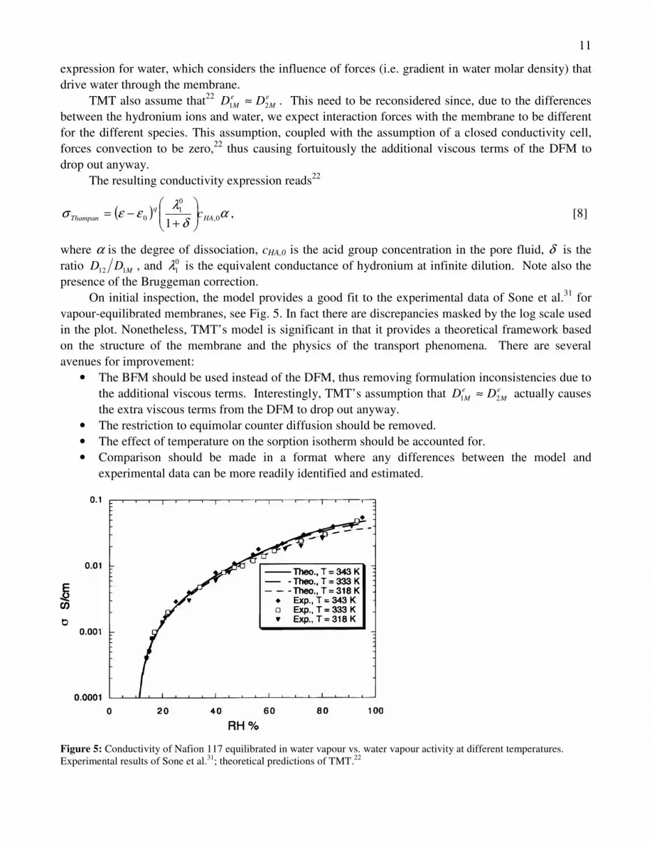
On initial inspection, the model provides a good fit to the experimental data of Sone et al.31 for vapour-equilibrated membranes, see Fig. 5. In fact there are discrepancies masked by the log scale used in the plot. Nonetheless, TMT’s model is significant in that it provides a theoretical framework based on the structure of the membrane and the physics of the transport phenomena. There are several avenues for improvement:

• The BFM should be used instead of the DFM, thus removing formulation inconsistencies due to the additional viscous terms. Interestingly, TMT’s assumption that e

MeM DD 21 ≈ actually causes

the extra viscous terms from the DFM to drop out anyway. • The restriction to equimolar counter diffusion should be removed. • The effect of temperature on the sorption isotherm should be accounted for. • Comparison should be made in a format where any differences between the model and

experimental data can be more readily identified and estimated.

Figure 5: Conductivity of Nafion 117 equilibrated in water vapour vs. water vapour activity at different temperatures. Experimental results of Sone et al.31; theoretical predictions of TMT.22

12

5 BINARY FRICTION MEMBRANE MODEL 5.1 Specialization of BFM to a PEM We now proceed to reduce the general binary friction model, Eqn. [4], to the binary friction membrane model (BFM2) by means of scaling arguments.

We consider transport within the family of perfluorosulfonic acid (PFSA) membranes, such as Nafion. The membrane is taken as the porous medium, and only two species are assumed present in the pore fluid, proton carriers (species i = 1) and water (i = 2). Furthermore we assume that the dominant proton carrier is hydronium.

The gradient in electrochemical potential (at constant temperature T) can be expressed as

( ) Φ∇+∇+∇+∇=∇ FzpXRT iiieiT iM,Vlnln γµ [9]

where the terms represent the effects of composition, activity, Gibb’s free energy, and electrical potential. Xi is the mole fraction, γi is the activity, VM,i is the specific molar volume, zi is the charge, and Φ is the ionic potential.

Introducing the above expression for the gradient of the electrochemical potential into the BFM and multiplying both sides by the mole fraction Xi , we obtain

( ) 2,1,ˆˆ

ˆ

ˆˆ

ˆ

ˆˆ

ˆˆˆˆˆv̂lnˆˆ

2

1i =+

��

���

��

���

−=Φ∇Θ+∇+∇+∇− =

iDcDc

X

Dc

XzXpXXX

iMt

i

j ijt

ji

ijt

ijiiiiii

NNNβγ [10]

In order to identify terms that may be neglected to simplify the numerical solution and to improve physical insight, the system in Eqn. [10] is written in dimensionless form using the parameters and variables found in Table 1. The reference molar densities are chosen to be the inverse of the partial molar volume of water, since this does not vary significantly with temperature or pressure. We assume the molar volumes for water and hydronium to be the same (see Section 5.4). Table 1: Non-Dimensional Quantities and Associated Reference Values Non-Dimensional Quantities Reference Values

Length MLxx =ˆ LM = membrane thickness Total mole density

reftt ccc =ˆ 33M,2 m mol 106.55V1 −−×==refc

Mole density of species i refii ccc =ˆ

Mole flux refii NNN ′=′ˆ refrefref cN v= , Mrefref LD=v

Molar volume

refM ,

M,221 V

Vv̂v̂ =≈ 2,, V

1V M

refrefM c

==

Diffusion coefficients

ref

eije

ijref

MSij

ij D

DD

D

DD ==

−

ˆ,ˆ eiM

MSijref DDD or ,−=

Pressure gradients ���

�

� ∆∇=∇

M

ref

L

ppp̂ˆ

25 m N 105 −×=∆ refp

Potential gradients ���

�

� ∆ΦΦ∇=Φ∇

M

ref

Lˆˆ

V 3.0=∆Φ ref

Gradient operator ∇=∇ mLˆ LM = membrane thickness

13

ref

ref

RTc

p∆=β

25 m N 105 −×=∆ refp Additional coefficients

RT

F ref∆Φ=Θ

V 3.0=∆Φ ref

5.2 Magnitude of the coefficients for the driving force terms To perform an order of magnitude analysis of the driving force terms, we assume, as a limiting case scenario, the pressure drop across the membrane to be 25 m N 105 −×=∆ refp , while the maximum potential drop across the membrane is approximately V 3.0=∆Φ ref .

Following previous studies22, we assume the gradients in composition are small and, thus, gradients in the activity coefficients are negligible, i.e. ( )0lnˆ ≅∇ iiX γ . Using the values in Table 1, the coefficients for the driving force terms are estimated in Table 2.

Table 2: Comparing the relative magnitude of the driving forces in the transport equations

Gradient of Interest

Coefficient for Gradient Term

Coefficient Value Approximate Order of

Magnitude

21ˆ,ˆ XX ∇∇ 1 1 ~1

β11v̂X ( )31 1015.3 −×X ~10-3

p̂∇̂ β22 v̂X ( )3

2 1015.3 −×X ~10-3

Φ∇ ˆˆ Θ1X ( )1.101X 1-10

As can be seen from the table, compared to the potential and mole fraction gradient terms, the pressure terms are of a significantly lower order and can be neglected. Also, the potential term is the dominant term when zi ≠ 0, while the gradient in mole fraction term is dominant when zi = 0.

Thus, Eqn. [8] can be reduced to

( ) 2,1,ˆˆ

ˆ

ˆˆ

ˆ

ˆˆ

ˆˆˆˆ

1

=+��

���

��

���

−=Φ∇Θ+∇− =

iDc

N

Dc

NX

Dc

NXzXX

iM

in

j ij

ji

ij

ijiii [11]

Expanding this for both species (i = 1, 2), using that52 jiij DD ˆˆ = , casting the above into matrix form, and inverting the matrix to obtain an expression for the fluxes in terms of the driving forces yields

����

�

�

�

∇

Φ∇Θ+∇

�����

�

�

�����

�

�

+

+

++

−−=��

�

�

�

2

11

112

2

12

2

12

1

212

1

21212

2

112

1

0

2

1

ˆ

ˆˆˆ

ˆ1

ˆˆ

ˆˆ1

ˆ

ˆˆ1

ˆˆˆˆ

)(ˆˆ

ˆ

X

XX

DD

X

D

X

D

X

DD

X

DDDD

X

DD

Xc

N

N

M

M

MeMMM

qεε. [12]

Here, we have also introduced the Bruggeman correction, Eqn. [7]. Note that Xi and ε depend on the water content λ, and the Dij are functions of λ and temperature

T. The next two sections will consider these dependencies in further detail.

14

5.3 Mole numbers, volumes, porosities etc. In the original presentation of the BFM2 model23, special attention was paid to computing the degree of dissociation of the sulfonate heads as a function of water content, α(λ). However, since i) almost all sulfonate heads dissociate as soon as the water content λ exceeds 2; ii) the conductivity vanishes at small values for λ; and iii) conditioned membranes in fuel cells maintain water contents above λ=2, it therefore reasonable and expedient to assume α = 1. The model is thus presented here with this simplification.

Due to electroneutrality, and since we assume that all sufonate heads are dissociated, the number of dissociated protons, n1, equals the number of sulfonate heads, n1 = nsh. Due to the definition of λ, the total number of water molecules is given by shw nn λ= , which implies that†

λw

sh

nnn ==1 [13]

We also have to account for the water molecules that are associated with protonated complexes. For a protonated complex containing ωpw water molecules, then ωpwn1 water molecules take part in the proton transport, while the remaining n2 = nw−ωpwn1 water molecules form the second species. For generality, the parameter ωpw could be retained in the model. However, as we are considering transport within vapour-equilibrated Nafion, it is reasonable to assume that hydronium is the protonated complex that is formed. Thus, we will assume ωpw =1 throughout, so that

��

�

� −=−=λ1

112 ww nnnn [14]

Next we determine the molar densities, which involve partial molar volumes. We could not find data on the exact partial molar volume of hydronium or other protonated complexes under the given conditions, i.e. within a hydrated membrane. In order to be able to progress, we make the reasonable assumption that the molar volume of water and hydronium is approximately the same,23,58 so that

2,1, VV MM = .

The volumes occupied by the protonated complex, the free waters, and the membrane are

λα

wnnV M,21M,21 VV == , ��

�

� −==λ1

1VV M,22M,22 wnnV , λ1

VV MM,MM, wshM nnV == [15]

where MM,V is the volume of membrane per mole of acid heads, dryEW ρ=MM,V ; ρdry is the dry density of the polymer membrane.

The total volume of pore fluid is, from Eqns. [15],

wp nVVV M,221 V=+= [16]

The mole densities of protonated complexes, free water within the pore fluid, and the total mole density of the pore fluid, are accordingly given by

λα

M,2

11 V

1==pV

nc , �

�

�

� −==λ

αλM,2

22 V

1

pVn

c , M,2

21 V1=+= ccct . [17]

This gives the mole fraction for the protonated complexes and the free waters as

† Obviously, this restricts the presented equations to values of λ>1, since for λ<1 one would, for the case of complete dissociation, expect n1 = nw.

15

λ11

1 ==tc

cX ,

λ1

122 −==

tcc

X . [18]

The porosity is defined as the volume of the pore fluid divided by the total volume, and, since the total volume is the sum of all volumes that make up the system, the porosity can be written as

M,2MM,21

21

V/V+=

+++

==λ

λεMt

p

VVVVV

V

V. [19]

The threshold porosity ε0 in the Bruggeman correction is defined by specifying a minimum water content λmin with ε0 = ε(λmin). Here λmin is the minimum amount of water that must be sorbed by the membrane for the pore liquid phase to be sufficiently well connected to allow for transport through the membrane. Examining the conductivity data in Figure 1, it is clear that λmin should lie somewhere between 1.5 and 2, since this is the approximate range where the conductivity bounds intersect the x-axis. 5.4 Diffusion coefficients The determination of the coefficients 12D , MD1 and MD2 , is required next. These coefficients depend on the PFSA material, and the state of the material, in particular on temperature T and water content λ.

One way to specify these coefficients is to fit their values to detailed measurements. This would require a painstaking effort involving systematic measurements covering all possible states of the membrane. Such measurements would be required anew for a new material.

Determination of the coefficients based on understanding of the membrane microstructure and modelling of the interaction between the membrane and the two transported species, i.e. hydronium and water, would be better. Most desirable would be a proper mathematical transition from an exact microscopic description of the interaction of membrane, hydronium and water, towards a macroscopic model. Such information and description being currently unavailable, we have to rely on guidance from knowledge on the membrane morphology to devise assumptions on the functional dependence of the coefficients on temperature and water content.

We assume the interaction between water and hydronium ions, as described by D12, does not depend on water content. This seems reasonable based on studies of the Stefan-Maxwell coefficients for systems of non-ideal fluids.51. Furthermore, since D12 represents binary diffusion within the fluid in the membrane, it should not depend on the water content λ. Thus, we can use the typical literature value, which at a temperature T0 = 303 K is denoted as 0

12D . In the absence of specific knowledge on species-membrane interaction, it is reasonable to assume

the interaction, D1M and D2M, depends on the water content due to changes in the geometry of the membrane, and the proximity of the species to the membrane. In order to determine the empirical fit of our model parameters, we assume a simple power law dependence, so that both D1M and D2M are increasing functions of λ. We introduce three dimensionless constants A1, A2, s and write

sM ADD λ1121 = and s

M ADD λ2122 = . [20]

The use of the same exponent, s, for both coefficients is a simplification; this could be refined by considering two separate exponents, s1 and s2.

Finally, we consider the temperature dependence. The coefficients Dij describe the interaction between two different species, and it is physically plausible to assume that the interaction becomes weaker with temperature. We will also adopt an Arrhenius law behaviour as in typical of thermally

16

activated interaction processes. As a first approximation, we assume that all three interaction coefficients vary in the same way, so that their temperature dependence is given through the temperature dependence of the coefficient D12, which we write as

( ) ��

���

����

�

�−==

TTRE

DTDD a 11exp

0

0121212 , [21]

where Ea is the activation energy. Again, a more refined theory could consider different Arrhenius laws for each of the three coefficients. 5.5 BFM2 Model The results of the last three sections can now be combined to yield the Binary Friction Membrane Transport Model (BFM2) which, after reinserting the dimensions, can be written as

�����

�

�

�

∇

Φ∇

�����

�

�

�����

�

�

−

−+

���

�

�+−+

−−=���

�

�

�

λλ

λ

λλλ

εε RTF

DD

DDD

DDDDDD

c

N

N

M

MM

MMMM

qt

112

2212

21212112

0

2

1

11

11

11

)( [22]

or, when we make all coefficients explicit, as

�����

�

�

�

∇

Φ∇

�����

�

�

�����

�

�

−

−+

���

�

�+−+

��

���

����

�

�−�

�

�

�

�−

+−

=���

�

�

�

−

−λ

λλ

λλ

λλλ

λλ

ελ

λRTF

A

AA

AAAA

TTRE

Dc

N

N

s

s

s

sss

a

q

t

1

22

1

122121

0

0120

M,2MM,

2

1

11

11

111

11exp

V/V [23]

The model contains six unknown constants, namely ε0 (or λmin), Ea, A1, A2, s, and q. These must be obtained by fitting to experimental data. While equations [22, 23] describe coupled transport of water and hydronium through a PFSA membrane, it is possible to determine the coefficients from conductivity measurements, in the absence of net water transport. This is possible because one of the characteristics of the BFM2 is that the constants that appear in the general BFM2 model are identical to those and in the simplified conductivity form of the model as will be shown next. Once determined from conductivity experiments, the constants can be reintroduced into the BFM2, and the model applied to compute coupled water and ionic transport.

6 BINARY FRICTION CONDUCTIVITY MODEL Conductivity is directly related to the transport of hydronium ions through the membrane, and is the best-documented transport property. In this section we reduce the BFM2 model, Eqn. [22]) to a conductivity model. It should be emphasized that this conductivity model is derived here primarily as a tool to gain insight into the behaviour of the unknown transport coefficients and to specify the model constants. 6.1 The conductivity model Conductivity measurements are commonly performed on membranes using AC impedance measurement techniques31. In such experiments, the membrane is generally considered to be uniformly

17

equilibrated with water vapour and thus that the gradient in water content is zero. It follows from Eqn. [22] that the protonic flux is then proportional to the potential gradient in the membrane as

( )( )( ) Φ∇

−+++

−−=RTF

DDDDDD

cNMM

MMqt 1

)(1122

122101 λλλ

λεε [24]

The ionic current density is related to the ionic fluxes by Faraday’s law

1

2

1

FNNzFii

ii == =

[25]

and conductivity is defined as

Φ∇−≡ iσ [26]

Using Eqns. [25] and [26], we obtain the Binary Friction Conductivity Model (BFCM)

( )( )( )1

)(1122

12212

0 −+++

−=λλλ

λεεσMM

MMqt DDD

DDDRTF

c , [27]

which, when the coefficients are specified according to the Sec. 5, can be written in explicit form as

( )( )( )s

sa

q

t AAAA

TTRE

RTFD

c −+−++

��

���

����

�

�−�

�

�

�

�−

+=

112

21

0

2012

0M,2MM, 1

11exp

V/V λλλλλε

λλσ [28]

Again we emphasize that Eqn. [27] is a reduction of [22] derived in the limit of negligible water

content gradient in the membrane (or in the limit of a negligible upper off-diagonal term ( ) MD21− ). Similarly to other established membrane models, Eqn. [27] does not account for the impact of water flux on protonic current. Its most useful feature in the context of the developments presented here is that it contains the same transport coefficients as the general BFM2, and thus any appropriate specification of parameters for the BFCM automatically and conveniently defines a set of parameters for the more general BFM2, which can than can be used to predict coupled protonic current and water fluxes as will be illustrated in Section 7.

6.2 Experimental Data Sone et al. 31 reported conductivity data for Nafion 117 in the E-form (no heat treatment), measured using a four-electrode AC impedance method. Membranes used in fuel cells are typically heated during the manufacture of the membrane electrode assembly, and it may thus be more appropriate to fit to the data for a membrane in the N or S form, however fitting to the E-form data allows direct comparison with Thampan et al. 22 fit to their model.

Sone et al’s data is measured in the plane of the membrane, but is expected to provide a reasonable measure of the normal direction conductivity since Nafion presents no apparent ordering of the macromolecules in any preferential direction, and its properties are expected to be reasonably isotropic. We also assume that the conductivity data measured by Sone and co-workers represents the conductivity of 1100 EW Nafion membranes of all thicknesses.

In Ref. 31 the conductivity data (in S cm-1) collected was fitted to a third degree polynomial, i.e.

18 32 xdxcxba SoneSoneSoneSoneSone +++=σ [29]

where x is the relative humidity ( )( )aTppx sat 100100 == , and the coefficients (aSone, bSone, cSone and dSone) are given for various temperatures. We will use the data for the E-form of Nafion for 30�C and 70�C.

An added complication is that the conductivity data of Sone et al. 31 is given as a function of the water vapour activity outside of the membrane. However, in the BFM2 and the BFCM, as well as in the models of Springer et al. 40 and Thampan et al.,22 conductivity is defined as a function of water contents λ. Casting conductivity as a function of λ, rather than activity, is more practical in applying the membrane model since λ is taken in general as varying throughout the membrane.

To convert the data of Sone et al.31 from a function of relative humidity x to a function of water content, we require the activity a as a function of water content λ. This is accomplished using a least squares fit of a third degree polynomial to fit the available sorption isotherm data from Sone et al.31 with λ as the independent variable and activity as the dependent variable. The resulting expression at 30°C is

34230 10149.30147.0232.0246.0 λλλ −×+−+−=Ca [30]

The largest standard error was found to be 03843.0=SE , and was added or subtracted from the least squares fit to estimate the error in our curve fit, SEaa Cerror

±= 30 .

Assuming the data a in Ref. 55 for 80°C is for a membrane with no heat-treatment (E-Form), and applying a similar procedure on Nafion 117 data at 80°C, we can fit a fourth order polynomial

443280 1060.50115.00685.00146.000562.0 λλλλ −×+−+++−=Ca [31]

The largest standard error in this case was found to be 0312.0=SE , with an error estimate for the fitting of SEaa Cerror

±= 80 .

We now have the data available to plot the conductivity as a function of the water content at 30 and 80°C. We will use the fitted sorption data at 80°C in our fitting of the BFCM below at 70°C.

6.3 Fitting conductivity The conductivity fit of Sone et al., Eqn. [29], was modified to plot the conductivity as a function of water content by using Eqns. [30, 31] at 30 and 70°C, respectively. The relative error was used as a guide to maintain the error within reasonable bounds while ensuring a fit within the range of conductivity values defined by the standard error in the sorption isotherms, and the resulting parameter values are

65.1min =λ , -12912 s m105.6 −×=D , 83.0=s , 5.1=q , 084.01 =A , 5.02 =A , K 1800=REa [32]

The minimum water content λmin was chosen such that the model conductivity threshold closely matches the data of Sone et al. A reasonable order of magnitude for D12 was chosen from a literature survey, and A1, A2, s, and D12 were then varied such that the BFCM results lay within the error bounds for all λ.

The coefficients A1 and A2 reflect the relative size of D1M and D2M respectively. Since the fitted value of A1 is much smaller than A2, this implies that the resistance of the membrane to hydronium diffusion is much large than to water. Given that hydronium ions have a net charge while water does not, this is reasonable since as we expect the interaction forces between the membrane (with charged

19

sulfonate heads) and the hydronium ions to be stronger than the forces between membrane and water. Sensitivity analysis shows23 that regardless of the order of magnitude of D12 the ratio of the values of D1M and D2M remains of the same order of magnitude, which is is encouraging in terms of the generality of the model.

� � � � � �� ��

�

�

�

�

�

�

λ (mol H O / mol SO )2 3-

Con

duct

ivity

(S

/ m

)

Upper bound

Lower bound

Figure 7: BFCM and anticipated upper and lower bounds on conductivity resulting from expected error in fit to sorption isotherm data at 30°C.

Figure 7 shows the fit of the BFCM to the experimental data, using the value of s = 0.8. The plot

fits within the anticipated range of conductivity values over almost the entire range of water contents, with the fit falling slightly outside the error bounds at a water content of approximately 5. At lower water contents (λ of about 2), the relative error is amplified by the small conductivity values, but the absolute error is in fact small.

The conductivity models of Refs. 22 and 40, Eqns. [3,8], are compared to the BFCM in Figure 8, which also shows the expected range of the data. Springer’s model‡ falls within the upper and lower bounds for high water contents λ, but outside for low values of λ. Thampan’s model falls within the upper and lower bounds for low water contents, but deviates significantly from the experimental results for higher water contents.

‡ Springer et al. omit to report whether the membrane considered was in the E-form or some heat-

treated form. Here we assume that it is for the E-form for comparison purposes.

20

� � � � � �� ��

�

�

�

�

�

�

λ (mol H O / mol SO )2 3-

Con

duct

ivity

(S /

m)

σ Upper bound

Lower bound

ThampanSpringer

Figure 8: Comparison of calculated conductivity using BFCM (solid) and models of Springer et al.40 and Thampan et al.22

against experimental data of Sone et al. 31 for E-form Nafion 117 at 30°C. For brevity, a direct comparison of the BFCM to the results using Thampan and Springer models

at 70°C is not presented here, but we note that Springer et al.’s model predictions are markedly inferior to those at 30°C. The minimum relative error is approximately 20% and the computed values lie outside the upper bound of conductivity range at all water contents. Possible causes for the large discrepancy in the Springer model predictions are discussed in Ref. 23. In any case, for this temperature, the BFCM exhibits again lower overall error for almost all water contents.

With the fitted parameters available at two temperatures, predictions at intermediate temperatures can be obtained to gauge the ability of the BFCM to correctly predict the temperature dependence of conductivity. Comparisons are made with Sone’s data at 45°C. One problem in attempting this is lack of reliable sorption isotherm data at temperatures near 45°C. This was remedied by implementing the chemical model of Weber and Newman developed for determining λ for a vapour-equilibrated membrane56 and used it to provide sorption isotherm data. A standard error of ±0.038 was used on the activity (the same standard error as was used at 30°C) to provide error bars within which conductivity is expected to lie.

As a reliability check, reliability of Weber and Newman’s chemical model was used to translate experimental conductivity data from a function of activity to a function of water content at 30, 70 and 80°C. For the case of 30°C, Weber and Newman’s conversion and the conversion using the fit to data overlap in the mid to high water content range. At lower water contents, the differences between the sorption isotherm model and the fit to the data for low water contents become more significant. In the conversion process for 70°C and 80°C, a significant overlap was noted for both temperatures over the entire range of water contents. The effect of a 10°C temperature variation on the sorption isotherms is small, and it was deemed23 that using the sorption data at 80°C to convert the conductivity data at 70°C is acceptable. Weber and Newman’s chemical model appears to provide a reasonable enough translation of the conductivity data, and should provide a useful basis to validate the temperature dependence behaviour of our model.

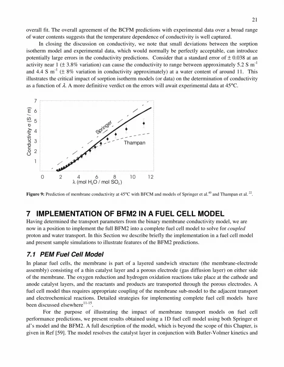
Figure 9 compares the model predictions to experiments at 45°C. Springer’s model falls outside the error across the range, while Thampan’s provides the best fit at very low water contents. Although the BCFM falls marginally outside the error bounds at high and low water contents, it provides a better

21

overall fit. The overall agreement of the BCFM predictions with experimental data over a broad range of water contents suggests that the temperature dependence of conductivity is well captured.

In closing the discussion on conductivity, we note that small deviations between the sorption isotherm model and experimental data, which would normally be perfectly acceptable, can introduce potentially large errors in the conductivity predictions. Consider that a standard error of ± 0.038 at an activity near 1 (± 3.8% variation) can cause the conductivity to range between approximately 5.2 S m-1 and 4.4 S m-1 (± 8% variation in conductivity approximately) at a water content of around 11. This illustrates the critical impact of sorption isotherm models (or data) on the determination of conductivity as a function of λ. A more definitive verdict on the errors will await experimental data at 45°C.

� � � � � �� ��

�

�

�

�

�

�

λ (mol H O / mol SO )2 3-

Con

duct

ivity

(S /

m)

σ

Thampan

Springer

Figure 9: Prediction of membrane conductivity at 45°C with BFCM and models of Springer et al.40 and Thampan et al. 22. 7 IMPLEMENTATION OF BFM2 IN A FUEL CELL MODEL Having determined the transport parameters from the binary membrane conductivity model, we are now in a position to implement the full BFM2 into a complete fuel cell model to solve for coupled proton and water transport. In this Section we describe briefly the implementation in a fuel cell model and present sample simulations to illustrate features of the BFM2 predictions.

7.1 PEM Fuel Cell Model In planar fuel cells, the membrane is part of a layered sandwich structure (the membrane-electrode assembly) consisting of a thin catalyst layer and a porous electrode (gas diffusion layer) on either side of the membrane. The oxygen reduction and hydrogen oxidation reactions take place at the cathode and anode catalyst layers, and the reactants and products are transported through the porous electrodes. A fuel cell model thus requires appropriate coupling of the membrane sub-model to the adjacent transport and electrochemical reactions. Detailed strategies for implementing complete fuel cell models have been discussed elsewhere11-15.

For the purpose of illustrating the impact of membrane transport models on fuel cell performance predictions, we present results obtained using a 1D fuel cell model using both Springer et al’s model and the BFM2. A full description of the model, which is beyond the scope of this Chapter, is given in Ref [59]. The model resolves the catalyst layer in conjunction with Butler-Volmer kinetics and

22

is solved numerically using a finite element method. One of the key issues in the implementation of the BFM2 in the fuel cell model is the coupling of the equation for water content (λ) to that for water mole fraction (Xw) in the porous electrode. This is dealt with using an iterative algorithm that enforces water conservation and allows the enforcement of the sorption isotherm at the membrane-catalyst interface59.

7.2 Effect of Membrane Transport on Fuel Cell Performance The direct effect of water content λ on predicted membrane conductivity can be assessed by setting the water transport to produce a linear profile of λ through the membrane, effectively producing a spatially varying membrane conductivity �m(λ). The anode water content is varied, while the cathode side is kept at λ = 14, and the total ohmic loss through the membrane computed using each model are plotted in Fig. 10 for a constant current density of i = 1 A/cm2. The membrane overpotential varies significantly between the three models, particularly at low anode water content. The BFM2 and Springer’s model are in close agreement for higher values of λ¸a. At lower values, the conductivity in the BFM2 is lower than the Springer model, but not as low as that obtained from Thampan et al’s model.

A clearer comparison of the two membrane models is presented in Figure 11, showing isocurrent lines obtained from simulations with constant voltage drop through the membrane, with varying anode and cathode water content at the boundaries. The voltage drop is specified as dV = 0.1 V. This corresponds to a current density of approximately 1.4 A/cm2 for a fully humidified membrane. As in Fig. 10, the models are similar at higher membrane humidification levels, but differ significantly at lower anode and/or anode water contents.

λ

mem

bran

eoh

mic

loss

es[V

]

2 4 6 8 10 12 14-0.5 -0.5

-0.45 -0.45

-0.4 -0.4

-0.35 -0.35

-0.3 -0.3

-0.25 -0.25

-0.2 -0.2

-0.15 -0.15

-0.1 -0.1

-0.05 -0.05

0 0

Springer, 80 CThampan, 80 Crevised BFM2, 80 C

Figure 10: Comparison of membrane overpotential for varying anode water contents. Membrane models: Springer et al.40, Thampan et al. 22 and BFM223

23

Figure 11: Current density contours computed using (left) model of Springer et al. and (right) BFM2. Computations performed for fixed membrane voltage drop of 0.1V. The overall impact of different humidification regimes is shown in Figure 12 in terms of the polarization curves obtained using the two models under two different humidification regimes: (i) dry cathode operation with 75% relative humidity (RH) on the anode and 25%RH on the cathode (labeled RH = 75/25); and (ii) dry anode with reversed conditions (labeled RH = 25/75). The Springer model predicts similar polarization curves for both regimes, while the BFM2 predicts a substantially larger polarization loss for the dry anode regime. The sensitivity of the BFM2 to the humidification regimes is physically realistic and should provide enhanced modelling reliability not only for low humidification conditions, such as those encountered in ambient air breathing fuel cells60, 61 and those relying on passive humidification schemes62, but also under typical fuel cell operating conditions in which local membrane drying is frequently encountered64.

Figure 12: Polarization curves obtained using Springer et al. model and BFM2 under dry cathode (RH = 75/25) and dry anode (RH = 25/75) conditions.

cell current [A/cm^2]

cell

volta

ge[V

]

0 0.2 0.4 0.6 0.8 1 1.2 1.40 0

0.2 0.2

0.4 0.4

0.6 0.6

0.8 0.8

Springer, RH = 75/25Springer, RH = 25/75BFM2, RH = 75/25BFM2, RH = 25/75

24

8 CLOSING REMARKS We have presented a review of experimental and macroscopic modelling aspects of transport phenomena in polymer electrolyte membranes. This included examination of the connection between the hydration scheme and the behaviour of the membrane, a discussion of the so-called Schroeder’s paradox, and the influence of the membrane phase on transport mechanisms. We also provided a critical examination of various approaches to modelling transport phenomena in membranes, and established that binary friction model provide a correct and rational framework for modelling membrane transport.

Based on this framework, a Binary Friction Membrane Model (BFM2) was developed to account for coupled transport of water and hydronium ions in polymer electrolyte membranes. The BFM2 was cast in a general form to allow for broad applicability to the PFSA family of membranes. As a tool to determine the model parameters, a simplified Binary Friction Conductivity Model (BFCM) was derived to represent conditions found in AC impedance conductivity measurements.

In order to validate the BFCM, we applied the model to 1100 EW Nafion. We used available conductivity and sorption data at 30°C and 70°C to determine the parameters of the conductivity model (Ea, λmin, D12, s, q, A1, A2). We then used this to predict the conductivity at 45°C. The overall agreement of the BCFM predictions with experimental data over a broad range of water contents suggests that the temperature dependence of conductivity is well captured. A more rigorous analysis of the temperature dependence would, however, require additional experimental data. Ideally sorption isotherm data and conductivity data, allowing for the determination of conductivity as a function of water content, should be obtained for a wider range of temperatures to allow for a more systematic analysis. Without detracting from the features of the BFCM, it should be noted that the predictive abilities of the classical models of Springer et al. and of Thampan et al. might also benefit from accounting for temperature dependence in the sorption isotherms.

One of the inherent advantages of the simplified BFCM is the ability to gain insight into the necessary transport parameters. A key feature is that the subset of transport coefficients determined from AC impedance measurements for the BFCM are the same as those appearing in the general BFM2. With additional data on water transport parameters (water diffusion coefficient and electro-osmotic drag), the fully specified BFM2 with all its required parameters was applied in a fuel cell model to account for coupled proton and water transport, and we presented results illustrating the enhanced predictive ability of the BFM2 compared to existing models, particularly in capturing the physics of lower humidity operation.

While the focus of the model performance assessment was on Nafion 1100 equivalent weight (EW), the binary friction membrane transport model is quite general and should be applicable to other PFSA membranes. This is supported by preliminary results in applying the model to Dow membranes and membrane C, whereby rational changes in a single model parameter based on physical considerations of structural differences from Nafion yield conductivity predictions that are in good agreement with experimental measurements63.

In order to apply the BFCM and the more general BFM2 to other membranes and to more systematically assess its performance for Nafion, detailed information and data are required, either from experiments or fundamental simulations. In addition to specification of the EW and the dry density of the membrane, or the molar volume (required for the porosity portion of the model), the model also requires specification, either from experiments or from a complementary dissociation model, of the fraction of dissociated acidic heads forming the charge carrying species.

25

The specification of the BFCM parameters (i.e. λmin, D12, s, A1, and A2) requires, at a minimum, conductivity data as a function of water content for a range of temperatures. Other relevant empirical data useful for implementing and assessing the general BFM2 are water diffusion coefficient through the membrane, and the electro-osmotic drag coefficient. As an alternative or supplement to empirical determination of the model parameters, it might be possible to obtain insight into these parameters from fundamental experiments or molecular dynamics simulations, and to elucidate, for example, the Dij

interaction terms. Acknowledgements This work was funded in part by grants to ND from the Natural Sciences and Engineering Research Council of Canada and the MITACS Network of Centres of Excellence. References 1. C Chuy, V. I. Basura, E. Simon, S. Holdcroft, J. Horsfall and K. V. Lovell, J. Electrochem. Soc.,

147, 4453 (2000). 2. J. Ding, C. Chuy and S. Holdcroft, Macromolecules, 35, 1348 (2002). 3. Kerres, J, Ullrich, A., Haring, T., Baldauf, M., Gebhardt, U. and W. Preidel, J. New Mat. Electr.

Sys., 3, 229 (2000). 4. J. Kerres, W. Cui, R. Disson and W. Neubrand, J. Membrane Sci., 139, 211 (1998). 5. C. Manea and M. Mulder, J. Membrane Sci. 206, 443 (2002). 6. M. K. Song, Y. T. Kim, J. M. Fenton, H. R. Kunz and H. W. Rhee. J. Power Sources, 117, 14

(2003). 7. V. I. Basura, C. Chuy, P. D. Beattie and S. Holdcroft, J. Electroanal. Chem., 501, 77 (2001). 8. O. Savadogo, J. New Mat. Electr. Sys., 1, 47 (1998). 9. J. J. Sumner, S. E. Creager, J. J. Ma and D. D. DesMarteau, J. Electrochem. Soc., 145, 107 (1998). 10. J. S. Wainright, J. T.Wang, D. Weng, R. F. Savinell and M. Litt, J. Electrochem. Soc., 142, L121

(1995). 11. T. Berning and N. Djilali, J. Electrochem. Soc., 150, A1589 (2003) 12. S. Um and C.Y. Wang, J. Power Sources, 125 (1), 40-51 (2004) 13. P.T. Nguyen, T. Berning and N. Djilali, J. Power Sources, 130 (1-2), 149 (2004) 14. A.Z. Weber and J. Newman, Chem. Rev., 104, 4679-4726 (2004) 15. B. Sivertsen and N. Djilali, J. Power Sources, 141 (1), 65-78 (2005) 16. K.D. Kreuer, S. Paddison, E. Spohr and M. Schuster, Chem. Rev., 104, 4637 (2004) 17. X. D. Din and E. E. Michaelides, AIChE J., 44, 35 (1998). 18. S. J. Paddison, R. Paul and T. A. Zawodzinski, J. Chem. Phys., 115, 7753 (2001). 19. R. Paul and S. J. Paddison, J. Chem. Phys., 115, 7762 (2001). 20. S. J. Paddison, R. Paul and T. A. Zawodzinski, J. Electrochem. Soc., 147, 617 (2000). 21. M. Eikerling, A. A. Kornyshev and U. Stimming, J. Phys. Chem. B, 101, 10807 (1997). 22. T. Thampan, S. Malhotra, H. Tang and R. Datta, J. Electrochem. Soc., 147, 3242 (2000). 23. J. Fimrite, B. Carnes, H. Struchtrup and N. Djilali, J. Electrochem. Soc., 152, A1815 (2005) 24. J. Fimrite, H. Struchtrup and N. Djilali, J. Electrochem. Soc., 152, A1804 (2005) 25. G. Inzelt, M. Pineri, J. W. Schultze and M. A. Vorotyntsev, Electrochim. Acta, 45, 2403 (2000).

26

26. M. Laporta, M. Pegoraro and I. Zanderighi, Phys. Chem. Chem. Phys., 1, 4619 (1999) 27. A. Z. Weber and J. Newman, J. Electrochem. Soc., 150, A1008 (2003). 28. K. D. Kreuer J. Membrane Sci., 185, 29 (2000) 29. T. A. Zawodzinski, T. E. Springer, J. Davey, R. Jestel, C. Lopez, J. Valerio and S. Gottesfeld, J.

Electrochem. Soc., 140, 1981 (1993). 30. K. D. Kreuer, Solid State Ionics, 97, 1 (1997). 31. Y. Sone, P. Ekdunge and D. Simonsson, J. Electrochem. Soc., 143, 1254 (1996). 32. P. Choi and R. Datta, J. Electrochem. Soc., 150, E601 (2003). 33. J. Elliot, S. Hanna, A. M. S. Elliot, and G. E. Cooley, Phys. Chem. Chem. Phys., 1, 4855 (1999). 34. A. Vishnyakov and A. V. Neimark, J. Phys. Chem. B, 104, 4471 (2000). 35. K. D. Kreuer, Solid State Ionics, 136, 149 (2000). 36. T. A. Zawodzinski, C. Derouin, S. Radzinski, R. J. Sherman, V. T. Smith, T. E. Springer and S.

Gottesfeld, J. Electrochem. Soc., 140, 1041 (1993). 37. K. D. Kreuer, Chem. Mater., 8, 610 (1996). 38. M. Eikerling, A. A. Kornyshev, A. M. Kuznetsov, J. Ulstrop and S. Walbran, J. Phys. Chem. B,

105, 3646 (2001). 39. T. A. Zawodzinski, J. Davey, J. Valerio and S. Gottesfeld, Electrochim. Acta, 40, 297 (1995). 40. T. E. Springer, T. A. Zawodzinski and S. Gottesfeld, J. Electrochem. Soc., 138, 2334 (1991). 41. P. Berg, K. Promislow, J. St-Pierre, J. Stumper and B. Wetton, J. Electrochem. Soc., 151, A341

(2004). 42. B. R. Breslau and I. F. Miller, Ind. Eng. Chem. Fund., 10, 554 (1971). 43. M. Verbrugge and D. Bernardi, AIChE J., 37, 1151 (1991). 44. M. Verbrugge and D. Bernardi, J. Electrochem. Soc., 139, 2477 (1992). 45. M. Verbrugge and R. F. Hill, J. Electrochem. Soc., 137, 1131 (1990). 46. M. Verbrugge and R. F. Hill, J. Electrochem. Soc., 137, 886 (1990). 47. M. Eikerling, Y. I. Kharkats, A. A. Kornyshev and Y. M. Volfkovich, J. Electrochem. Soc., 145,

2684 (1998). 48. T. Fuller and J. Newman, J. Electrochem. Soc., 140, 1218 (1993). 49. D. M. Bernardi, J. Electrochem. Soc., 137, 3344 (1990). 50. G. J. M. Janssen, J. Electrochem. Soc., 148, A1313 (2001). 51. R. Taylor and R. Krishna, Multicomponent Mass Transfer, John Wiley & Sons, Toronto (1993). 52. P. J. A. M. Kerkhof, Chem. Eng. J., 64, 319 (1996). 53. E. A. Mason and A. P. Malinauskas, Gas Transport in Porous Media; The Dusty Gas Model,

Elsevier, Amsterdam (1983). 54. R. Krishna and J. A. Wesselingh, Chem. Eng. Sci., 52, 861 (1997). 55. D. R. Morris and X. Sun, J. Appl. Polym. Sci., 50, 1445 (1993). 56. J. T. Hinatsu, M. Mizuhata and H. Takenaka, J. Electrochem. Soc., 141, 1493 (1994). 57. A. Z. Weber and J. Newman, J. Electrochem. Soc., 151, A311 (2004). 58. B. E. Conway, Ionic Hydration In Chemistry and Biophysics, Elsevier Scientific Publishing

Company, Netherlands (1981).

27

59. B. Carnes and N. Djilali, Modelling and Simulation of Conduction of Protons and Liquid Water in a Polymer Electrolyte Membrane Using the Binary Friction Membrane Model, IESVic Report, University of Victoria ( (2005)

60. W. Ying, Y.J. Sohn, W.Y Lee, J. Ke and C.S Kim, J. Power Sources, 145, 563-571 (2005) 61. S. Litster, J.G. Pharoah, G. McLean and N. Djilali, J. Power Sources, IN PRESS (2005) 62. Y. Wang and C.Y. Wang, J. Power Sources, IN PRESS (2005) 63. J. Fimrite, Transport Phenomena in Polymer Electrolyte Membranes, MASc Thesis, University of

Victoria (2004). 64. J. Stumper, M. Löhr and S. Hamada, Proc. Int. Symp. Fuel Cell & Hydrogen Technologies,

MetSoc, Calgary, Canada, 531 (2005).