Covariant gauge-invariant perturbations in multifluid f(R) gravity

arX

iv:1

110.

1191

v3 [

gr-q

c] 7

Jun

201

2

Covariant gauge-invariant perturbations in

multifluid f(R) gravity

Amare Abebe 1,2‡, Mohamed Abdelwahab 1,2 , Alvaro de la

Cruz-Dombriz1,2 and Peter K. S. Dunsby1,2,3

1 Astrophysics, Cosmology and Gravity Centre (ACGC), University of CapeTown, Rondebosch, 7701, South Africa2 Department of Mathematics and Applied Mathematics, University of CapeTown, 7701 Rondebosch, Cape Town, South Africa3 South African Astronomical Observatory, Observatory 7925, Cape Town,South Africa.

Abstract. We study the evolution of scalar cosmological perturbations in the1 + 3 covariant gauge-invariant formalism for generic f(R) theories of gravity.Extending previous works, we give a complete set of equations describing theevolution of matter and curvature fluctuations for a multi-fluid cosmologicalmedium. We then specialize to a radiation-dust fluid described by barotropicequations of state and solve the perturbation equations around a backgroundsolution of Rn gravity. In particular we study exact solutions for scales muchsmaller and much larger than the Hubble radius and show that n > 2

3in order to

have a growth rate compatible with the Meszaros effect.

PACS numbers: 98.80.-k, 04.50.Kd, 95.36.+x

‡ [email protected]

http://arxiv.org/abs/1110.1191v3

Covariant gauge-invariant perturbations in multifluid f(R) gravity 2

1. Introduction

There are at least three areas where standard General Relativity (GR) theory facesserious challenges from other competing fundamental theories [1]. Firstly, attemptsto unite quantum mechanics with GR have so far been unsuccessful and with theremarkable success the former has achieved over the last hundred years, many arequestioning the unique status of GR, suggesting that a fundamental modification ofthe theory could lead to a complete description of gravity on all scales. Secondly,in standard particle physics all the forces of nature save gravity have been shown tobe manifestations of an underlying unified theory of nature and there are hopes thatmodifications of GR could lead to a grand unification of all the known forces into asingle theory of everything. Thirdly and most important to us here is the missing linkbetween the observed universe and the standard theory of cosmology.

The recent discovery of the accelerated expansion of the Universe has cast a newshadow on the simplest cosmology based on Einstein’s theory of GR, together with aconventional matter description. Observational analyses [2]-[6] show that only a tinyfraction (∼ 4%) of the energy content of the Universe is known to exist in normalmatter form, whereas ∼ 23% of it exists in a little understood dark matter form.Dubbed as Dark Energy (DE), the remaining (∼ 72%) of the energy content of theUniverse is believed to be the cause of the inferred accelerated cosmic expansion.

Many candidates have been put forward as an explanation for DE, but most ofthem fall under one of these three forms: the cosmological constant, exotic scalarfields (such as Quintessence) and geometrical dark energy in which the gravitationalLagrangian is modified with respect to the usual Einstein-Hilbert one (see [7], [8], [9]and [10] for an extensive review).

An important class of modified gravity are the scalar-tensor and f(R) theories[11]-[23]. Both these candidates have their own serious shortcomings [17, 18, 19],and have to pass rigorous theoretical and observational scrutiny before they canbe accepted as viable theories [24, 25]. In this work we will only concentrate onthe interpretation of DE as geometrical manifestation of a more fundamental theory,focusing on f(R)-gravity.

It is well known that the dynamical evolution of small density perturbations,seeded in the early Universe, led to the large-scale structure we see today [26]-[36].An excellent framework for studying cosmological perturbations is the 1+3 covariantapproach, which has been developed, among other things, to analyze the evolutionof linear perturbations of Friedmann-Lemaıtre-Robertson-Walker (FLRW) models inGR [37] - [46].

In recent years, higher order theories of gravity have attracted a great deal ofattention. A detailed analysis of the background FLRW models using dynamicalsystem techniques has shown that there exist classes of fourth order theories whichadmit a transient decelerated expansion phase during which structure formation cantake place, followed by a DE-like era which drives the present cosmological acceleration(see [47] among many others). However, it has been proved [48] that when dustmatter scalar cosmological perturbations are studied in the metric formalism, f(R)theories, even mimicking the standard cosmological expansion, provide a differentmatter power spectrum from that predicted by the ΛCDM model [49]. In [51]the evolution of scalar perturbations of FLRW models in fourth order gravity wasdeveloped for single barotropic fluids using the 1+3 covariant approach and thesolutions of the perturbation equations on large-scales showed that a decelerated phase


is not necessarily required to form large scale structures. This divergence from thestandard GR provides us with a distinguishable signature of fourth order theories,which can be tested against observations.

However, since the Universe consists of a mixture of fluids, a complete treatment ofperturbations in fourth order theories requires taking this into account. The aim of thispaper is therefore to present a general framework for studying multi-fluid cosmologicalperturbations with a completely general equation of state in a f(R) theory of gravity,using the 1+3 covariant approach.

This paper has been organized as follows: in section 2 we give the general outlineof the 1+3 covariant approach. In section 3 we discuss the choice of frame and definethe key variables used in the description of perturbations in the total fluid and theindividual fluid components. Equations for these variables are given in section 4. Insections 5 and 6, respectively, the scalar and the harmonically decomposed forms ofour equations are presented. Applications to a radiation-dust cosmological mediumare given in section 7, with sections 8 and 9 devoted to the analysis of the short andlong wavelength limits of the perturbation equations. We conclude the paper by givingour conclusions in section 10.

The natural unit conventions (~ = c = kB = 8πG = 1) are in use. Latin indices oftensors run from 0 to 3. The symbols ∇ and ; represent the usual covariant derivative,∂ corresponds to partial differentiation and an over-dot shows differentiation withrespect to proper time. We use the (−+++) spacetime signature in this work.

For an arbitrary f(R) gravity the generalized Einstein-Hilbert action can bewritten as

Af(R) =1

2

∫

d4x√−g (f(R) + 2Lm) . (1)

A generalization of the Einstein’s Field Equations (EFEs) derived by varying thisaction with respect to the metric takes the form

f ′Gab = Tmab +

1

2gab(f −Rf ′) +∇b∇af

′ − gab∇c∇cf ′ , (2)

where f ≡ f(R), f ′ ≡ dfdR

and Tmab ≡ 2√−g

δ(√−gLm)δgab

.

Defining the energy momentum tensor of the curvature “fluid” as

TRab ≡

1

f ′

[

1

2(f −Rf ′)gab +∇b∇af

′ − gab∇c∇cf ′]

, (3)

the field equations (2) can be written in a more compact form

Gab = Tmab + TR

ab ≡ Tab, (4)

where the effective energy momentum tensor of standard matter is given by

Tmab ≡ Tm

ab

f ′ . (5)

Assuming that the energy-momentum conservation of standard matter Tmab

;b = 0holds, leads us to conclude that Tab is divergence-free, i.e., Tab

;b = 0, and thereforeTmab and TR

ab are not individually conserved [51]:

Tmab

;b =Tmab

;b

f ′ − f ′′

f ′2TmabR

;b , TRab

;b =f ′′

f ′2TmabR

;b . (6)


2. Covariant Decomposition of 4th-order Gravity

2.1. Preliminaries

The standard perturbation theory based on the metric formalism has disadvantageswhen it comes to extracting physical information from the perturbation variables. Forexample, it requires a complete specification of the correspondence between the lumpy,perturbed universe and the background spacetime. In other words, this approach isgauge-dependent. In this paper we instead use the 1+3-covariant formalism, a fluidapproach, which, when applied to cosmological perturbations leaves no unphysicalmodes in the evolution of the fluctuations: it requires no prior metric specificationand is gauge-invariant by construction.

2.2. Kinematics

We project onto surfaces orthogonal to the 4-velocity of the fluid flow using theprojection tensor hab ≡ gab + uaub and ∇a = hb

a∇b is the spatially totally projectedcovariant derivative operator orthogonal to ua. The covariant convective and spatialcovariant derivatives on a scalar function X are respectively given by

X = ua∇aX, ∇aX = hab∇bX . (7)

The geometry of the flow lines is determined by the kinematics of ua:

∇bua = ∇bub − aaub , (8)

∇bua = 13Θhab + σab + ωab . (9)

From (8) and (9) we obtain an important equation relating our key kinematicquantities:

∇bua = −ubua +13Θhab + σab + ωab , (10)

The RHS of this equation contains the acceleration of the fluid flow ua, expansion Θ,shear σba and vorticity ωba.

Another key equation is the propagation equation for the expansion - theRaychaudhuri equation (given here for the FLRW background) :

Θ +1

3Θ2 +

1

2(µ + 3p) = 0 , (11)

where µ and p hold for the total energy density and isotropic pressure respectively.This equation together with the equation of state p = p(µ, s), the energy conservationequation

µ+ Θ(µ+ p) = 0 , (12)

and the Friedmann equation

Θ2 +9K

a2− 3µ = 0 , (13)

form a closed system of equations and completely characterize the kinematics of thebackground cosmological model.

In this paper angular brackets denote the projection of a tensorial quantity ontothe tangent 3-space. Thus the relations

V〈a〉 = habVb , (14)

W〈ab〉 =[

h(achb)

d − 13h

cdhab

]

Wcd (15)

give the projection of a vector Va and the projected, trace-free part of a tensor Wab

respectively.


3. Matter Description

3.1. Effective Total Energy-Momentum Tensor

The thermodynamical description of a relativistic fluid is dictated by the energymomentum tensor Tab, the particle flux Na and the entropy flux Sa of the system.Whereas T ab and Sa always satisfy respectively the conservation of 4-momentum andthe second law of thermodynamics, namely

T ab;b = 0 , Sa

;a ≥ 0 , (16)

particle flux conservation, i.e., Na;a = 0, may be violated.

The total energy-momentum tensor in a general frame is sourced by µ, p, theenergy flux q〈a〉, and the anisotropic pressure π〈ab〉:

Tab = µuaub + phab + 2q(aub) + πab = Tmab + TR

ab . (17)

It defines our thermodynamical quantities:

µtot = T totab uaub = µm + µR , (18)

ptot =1

3T totab hab = pm + pR , (19)

qtota = −T totbc hb

auc = qma + qRa , (20)

πtotab = T tot

cd hc〈ah

db〉 = πm

ab + πRab , (21)

where µm = µm

f ′, pm = pm

f ′, qma =

qma

f ′, and πm

ab =πm

ab

f ′are the effective

thermodynamic quantities of matter.If we impose the Strong Energy Condition TabV

aV b ≥ 0 for all timelike vectorsV a, then Tab will have a unique unit timelike vector ua

E (uaEu

Ea = −1). Another

timelike vector uaN can be defined along the flux Na

N , i.e., uaN = Na√

−NbNb.

For a perfect fluid (or an unperturbed fluid in the background space), uaE , u

aN

and Sa are all parallel [38] and a unique hydrodynamic 4-velocity ua can be definedfor the fluid flow, in which case

Tab = µuaub + phab , Na = nua, Sa = sua , (22)

where µ and p are related by the equation of state p = p(µ, s). n = −Naua ands = −Sau

a define the particle and entropy densities respectively in the local restframe of an observer attached to ua.

We can also decompose the EMT with respect to another frame, say na, but inthis case we need to introduce a particle drift ja = ha

bNa [38, 40, 52].

If the fluid is imperfect, the fluid hydrodynamic 4-velocity is no longer uniqueand our EMT will take the more general form given above Eqn. (17) and the particleflux includes a drift term:

Na = nua + ja . (23)

Choosing the relevant frame is a crucial step in the covariant formulation ofperturbation theories, since ua is the velocity of fundamental observers in the Universe§.§ Fluid flow vector ua is uniquely defined as the future directed timelike eigenvector of the Riccitensor: ua = dx

a

dτ, where xa(τ) describes the worldline of the fluid in terms of the proper time τ . In

our multi-fluid picture, it corresponds to the normal to the surface of homogeneity.


In the particle frame ua = uaN , called the Eckart choice, an observer Ou=uN

seesno particle drift and hence ja = jaN = 0. If, on the other hand, we consider the energyframe ua = ua

E, also known as the Landau choice, an observer OuEmeasures no energy

flux (qa = qEa = 0) along the flow line and the EMT takes the form (22).For multi - component matter fluids we have

Tmab =

∑

i

T iab , (24)

where

T iab = µiu

iau

ib + pih

iab + qiau

ib + qibu

ia + πi

ab , (25)

hiab = gab + ui

auib , (26)

Nai = niu

ai + jai , (27)

uia being the normalized fluid 4-velocity vector for the ith component, ua

i uia = −1,

which we can fix by either choosing the energy frame uai = ua

Ei thereby settingqai = qaEi = 0, or the particle frame ua

i = uaNi for which jai = jaNi = 0 for that

component. The velocity of the ith fluid component relative to the fundamentalobserver Ou is defined to be

V ai ≡ ua

i − ua . (28)

V ai 6= 0 for tilted, inhomogeneous cosmological media whereas the special case

where uai coincides with ua describes an untilted homogeneous cosmological medium.

Decomposition of the matter stress-energy tensor with respect to the 4-velocity ua

gives the following thermodynamical quantities:

µm = Tmabu

aub =N∑

i=1

µi , (29)

pm =1

3Tmabh

ab =

N∑

i=1

pi , (30)

qma = −Tmbc h

bau

c =

N∑

i=1

(µi + pi)Via , (31)

πmab = Tm

cdhc〈ah

db〉 = 0 (to first order). (32)

In a similar way we can decompose the energy momentum tensor of the curvature fluidto obtain the corresponding thermodynamical quantities (denoted in what follows bya R superscript or subscript). All these quantities, unlike their matter counter-parts,vanish in standard GR, with a FLRW geometry:

µR = TRabu

aub =1

f ′

[

1

2(Rf ′ − f)−Θf ′′R+ f ′′∇2R

]

, (33)

pR =1

3TR

abhab =

1

f ′

[

1

2(f −Rf ′) + f ′′R+ f ′′′R2

+2

3

(

Θf ′′R− f ′′∇2R− f ′′′∇aR∇aR)

]

, (34)


qRa = −TRbch

bau

c = − 1

f ′

[

f ′′′R∇aR + f ′′∇aR− 1

3f ′′Θ∇aR

]

, (35)

πRab = TR

cdhc〈ah

db〉 =

1

f ′

[

f ′′∇〈a∇b〉R+ f ′′′∇〈aR∇b〉R− σabR]

. (36)

In the background FLRW universe, V ai = 0 and all perfect fluid components have

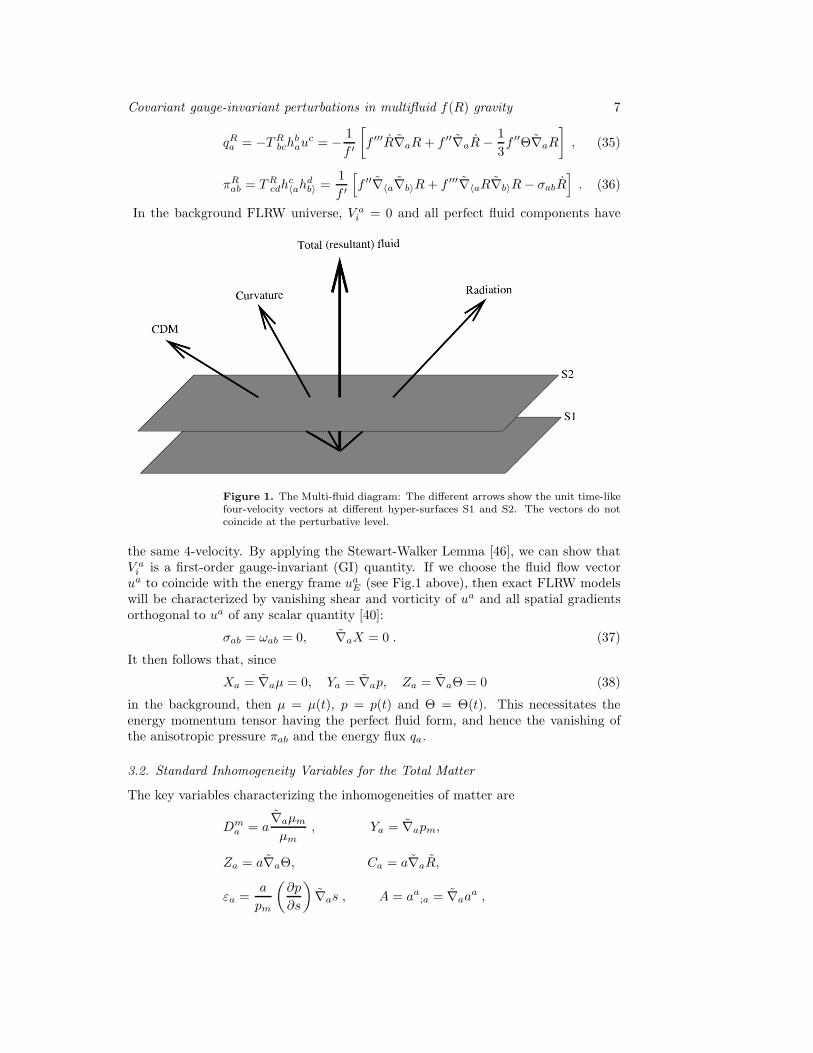
Figure 1. The Multi-fluid diagram: The different arrows show the unit time-likefour-velocity vectors at different hyper-surfaces S1 and S2. The vectors do notcoincide at the perturbative level.

the same 4-velocity. By applying the Stewart-Walker Lemma [46], we can show thatV ai is a first-order gauge-invariant (GI) quantity. If we choose the fluid flow vector

ua to coincide with the energy frame uaE (see Fig.1 above), then exact FLRW models

will be characterized by vanishing shear and vorticity of ua and all spatial gradientsorthogonal to ua of any scalar quantity [40]:

σab = ωab = 0, ∇aX = 0 . (37)

It then follows that, since

Xa = ∇aµ = 0, Ya = ∇ap, Za = ∇aΘ = 0 (38)

in the background, then µ = µ(t), p = p(t) and Θ = Θ(t). This necessitates theenergy momentum tensor having the perfect fluid form, and hence the vanishing ofthe anisotropic pressure πab and the energy flux qa.

3.2. Standard Inhomogeneity Variables for the Total Matter

The key variables characterizing the inhomogeneities of matter are

Dma = a

∇aµm

µm

, Ya = ∇apm,

Za = a∇aΘ, Ca = a∇aR,

εa =a

pm

(

∂p

∂s

)

∇as , A = aa;a = ∇aaa ,


Aa = ∇aA , Q = qa ;a ≃ ∇aq , (39)

where a ≡ a(t) here is the usual FLRW cosmological scale factor. Dma and Za define

the comoving fractional density gradient and comoving gradient of the expansionrespectively and can in principle be measured observationally [40]. The relation

pεa =∑

i

piεia +

1

2

∑

i,j

hihj

h(c2si − c2sj)S

ija (40)

defines the dimensionless variable εa that quantifies entropy perturbations in the totalfluid. We have defined the shorthand h ≡ µm + pm for the total matter fluid andhi ≡ µi+pi for the component matter fluids. w and c2s denote the effective barotropicequation of state and speed of sound of the total matter fluid, respectively, and aredefined by

w ≡ pmµm

, c2s ≡ ∂pm∂µm

, (41)

whereas for each component mater fluid, these two quantities are given by wi ≡ pi/µi

and c2si ≡ ∂pi/∂µi.

3.3. Matter Inhomogeneity Variables for the Components

The variables characterizing inhomogeneities of matter for the ith- component fluidare defined as

Dia = a

∇aµi

µi

, Y ia = ∇api , εia =

a

pi

(

∂pi

∂si

)

∇asi . (42)

In near-perfect fluid analyses such as the present one, εia is often taken to be negligible.Thus in subsequent discussions all terms containing this quantity are dropped.

3.4. Curvature Fluid Variables

The information about our deviation from standard GR is carried by the followingdimensionless gradient quantities

Ra = a∇aR , ℜa = a∇aR . (43)

These variables describe the inhomogeneities in the Ricci scalar. Finally, the velocityof the curvature fluid is defined, following [39], by

V Ra = −∇aR

R, (44)

provided that R 6= 0. Cases with constant scalar configurations or pathologic f(R)models with points of inflection in R(t) are excluded from this analysis.

4. Equations in the Energy Frame

We now derive the time evolution of the perturbations to linear order in the energyframe of the matter, i.e., in the frame where ua = ua

m.


4.1. Total Fluid Equations

These equations characterize the temporal fluctuations of inhomogeneities in a genericperfect cosmological fluid with an equation of state evolving as w = (1+w)(w− c2s)Θ.They are the following:

Da + (1 + w)Za − wΘDa = 0 , (45)

Za −(

Rf ′′

f ′ − 2

3Θ

)

Za −[

(1 + 3w)c2s − 2(1 + w)

2(1 + w)

µm

f ′ +2c2sΘ

2 + 3c2s(µR + 3pR)

6(1 + w)

+c2s

1 + w

2K

a2

]

Dma −

[

2f ′Θ2 + 3(1 + 3w)µm + 3f ′(µR + 3pR)

6f ′(1 + w)+

1

1 + w

2K

a2

]

wεa

−Θf ′′

f ′ ℜa −[

1

2− 1

2

ff ′′

f ′2 +f ′′µm

f ′2 − RΘ

(

f ′′

f ′

)2

+ RΘf ′′′

f ′ +2K

a2f ′′

f ′

]

Ra

+f ′′

f ′ ∇2Ra +

c2s∇2Dma

1 + w+

w∇2εa1 + w

= 0 , (46)

Ra −ℜa + R

[

c2s1 + w

Da +w

1 + wεa

]

= 0 , (47)

ℜa +

(

2Rf ′′′

f ′′ +Θ

)

ℜa −[

(1− 3c2s)µm

3f ′′ − c2s1 + w

R

]

Da +

(

wµm

f ′′ +w

1 + wR

)

εa

+ RZa +

(

2K

a2+ R

f ′′′

f ′′ + R2 f(iv)

f ′′ + RΘf ′′′

f ′′ +1

3

f ′

f ′′ −R

3

)

Ra − ∇2Ra = 0 . (48)

The linearized 3-curvature scalar of the projected metric hab orthogonal to the4-velocity vector ua is [38]

R = 2

(

−1

3Θ2 + µ

)

(49)

reduces to the Ricci scalar in the hypersurfaces orthogonal to ua when ω = 0. Thecovariant, GI gradient Ca gives, to linear order

Ca

a2+

(

4

3Θ + 2

Rf ′′

f ′

)

Za − 2µm

f ′ Dma + 2Θ

f ′′

f ′ ℜa − 2f ′′

f ′ ∇2Ra

+

[

2ΘRf ′′′

f ′ − f ′′

f ′

(

f

f ′ − 2µm

f ′ + 2RΘf ′′

f ′ +4K

a2

)]

Ra = 0 . (50)

This variable quantifies the spatial variation in the 3-curvature and is ageometrically natural quantity useful in the long wavelength analysis of ourperturbation equations. The time evolution of this quantity is given by

Ca = 2K

{

3f ′Ca

a2(2Θf ′ + 3Rf ′′)+Dm

a

[

8wΘ

3(1 + w)− 2f ′Θ2 − 6f ′µR

2Θf ′ + 3Rf ′′

]

− 6f ′′∇2Ra

2Θf ′ + 3Rf ′′

−

a2(Θf ′′ − 3Rf ′′′)

3f ′

12RΘf ′f ′′′ − 2f ′′(

3f − 2Θ2f ′ + 6Θ2µR + 6RΘf ′′)

2Θf ′ + 3Rf ′′

Ra


+

[

6Θf ′′

2Θf ′ + 3Rf ′′ +f ′′

f ′

]

ℜa

}

+K2

[

36f ′′Ra

a2(2Θf ′ + 3Rf ′′)− 36f ′Dm

a

a2(2Θf ′ + 3Rf ′′)

]

+2

3∇2

{

2wa2Θ

(1 + w)Dm

a +a2

f ′

[

3f ′′ℜa − (Θf ′′ − 3Rf ′′)Ra

]

}

. (51)

4.2. Component Equations

These are the equations that describe the evolution dynamics of the individual fluidcomponent fluctuations. For the component matter and velocity fluctuations, theseare given by

Dia − (wi − c2si)ΘDi

a + (1 + wi)Za =1

µihhiΘ(c2sµDa + pεa)− a(1 + wi)∇a∇bV i

b ,(52)

V ia −

(

c2si −1

3

)

ΘV ia =

1

ahhi

(

hic2sµDa + hipεa − hc2siµ

iDia

)

. (53)

We note that the equations involving the gradients of the inhomogeneities in theexpansion and curvature variables (Za,Ra,ℜa, Ca) remain the same as in the totalfluid equations (46)-(51). This is to be expected since these quantities are globalintrinsic properties of the spacetime itself rather than of the individual components ofmatter in the fluid.

4.3. Relative Equations

Let us now define the variables that relate features of pairs of the different componentsof the fluid, and derive their governing evolution equations. These relative variablesdepend only on the choice of the individual velocities, not on the choice of the overallframe.

Sija ≡ µiD

ia

hi

− µjDja

hj

, V ija ≡ V i

a − V ja . (54)

These are the quantities that allow us to distinguish between adiabatic and isothermalperturbations [27, 38].

The derivation of the evolution equations for the above quantities isstraightforward and yields

V ija − (c2sj − 1

3 )ΘV ija − (c2si − c2sj)ΘV i

a = − 1

ahi

(c2si − c2sj)µiDmi − 1

ac2sjS

ija , (55)

Sija + a∇a∇bV ij

b = 0 . (56)

5. Scalar Equations

The quantities we have considered so far contain both a scalar and a vector (solenoidal)part. Structure formation on cosmological scales is believed to follow sphericalclustering and therefore we present here the spherically symmetric, scalar densityperturbations obtained by taking the divergence of the gradient quantities. In sodoing, we first apply a local decomposition

a∇bXa = Xab =13habX +ΣX

ab +X[ab] , (57)


where ΣXab = X(ab) − 1

3habX describes shear whereas X[ab] describes the vorticity.Vorticity and shear describe the rotation and distortion of the density gradient field,respectively. The above decomposition extracts the scalar part of the perturbationvectorial gradients. Accordingly, when extracting the scalar contribution the vorticityterm vanishes [50].

5.1. Scalar Variables

On the basis of the above decomposition scheme, our scalar variables are:

∆m = a∇aDma , Z = a∇aZa , C = a∇aCa , R = a∇aRa ,

ℜ = a∇aℜa , ε = a∇aεa , ∆im = a∇aDi

a , Vi = a∇aV ia ,

Sij = a∇aSija , Vij = a∇aV ij

a . (58)

The scalar variables describing the total fluid will thus evolve according to

∆m + (1 + w)Z − wΘ∆m = 0 , (59)

Z −(

Rf ′′

f ′ − 2

3Θ

)

Z −[

1

2− 1

2

ff ′′

f ′2 +f ′′µm

f ′2 − RΘ

(

f ′′

f ′

)2

+ RΘf ′′′

f ′

]

R

+f ′′

f ′ ∇2R−

[

(1 + 3w)c2s − 2(1 + w)

2(1 + w)

µm

f ′ +2c2sΘ

2 + 3c2s(µR + 3pR)

6(1 + w)

]

∆m

−[

2f ′Θ2 + 3(1 + 3w)µm + 3f ′(µR + 3pR)

6f ′(1 + w)

]

wε−Θf ′′

f ′ ℜ+c2s

1 + w∇2∆m

+w

1 + w∇2ε = 0 , (60)

R − ℜ+ R

(

c2s1 + w

∆m +w

1 + wε

)

= 0 , (61)

ℜ +

(

2Rf ′′′

f ′′ +Θ

)

ℜ+

(

Rf ′′′

f ′′ + R2 f(iv)

f ′′ + RΘf ′′′

f ′′ +1

3

f ′

f ′′ −R

3

)

R− ∇2R

+ RZ −[

(1 − 3c2s)µm

3f ′′ − c2s1 + w

R

]

∆m +

[

wµm

f ′′ +w

1 + wR

]

ε = 0 , (62)

C

a2+

(

4

3Θ + 2

Rf ′′

f ′

)

Z +

[

2ΘRf ′′′

f ′ − f ′′

f ′

(

f

f ′ − 2µm

f ′ + 2RΘf ′′

f ′

)]

R

− 2µm

f ′ ∆m + 2Θf ′′

f ′ ℜ− 2f ′′

f ′ ∇2R = 0 . (63)

The evolution of the constraint equation is given by

C = K

{

6f ′C

a2(2Θf ′ + 3Rf ′′)+ ∆m

[

16wΘ

3(1 + w)− 4f ′Θ2 − 12f ′µR

2Θf ′ + 3Rf ′′

]

− 12f ′′∇2R2Θf ′ + 3Rf ′′

−

2a2(Θf ′′ − 3Rf ′′′)

3f ′

12RΘf ′f ′′′ − 2f ′′(

3f − 2Θ2f ′ + 6Θ2µR + 6RΘf ′′)

2Θf ′ + 3Rf ′′

R


+

(

12Θf ′′

2Θf ′ + 3Rf ′′ +2f ′′

f ′

)

ℜ}

+K2

[

36f ′′Ra2(2Θf ′ + 3Rf ′′)

− 36f ′∆m

a2(2Θf ′ + 3Rf ′′)

]

+ ∇2

[

4wa2Θ

3(1 + w)∆m +

2a2f ′′

f ′ ℜ− 2a2(Θf ′′ − 3Rf ′′)

3f ′ R]

. (64)

For the scalar variables describing component inhomogeneities and interactions in thefluid, the evolution equations are given by

∆im −Θ(wi − c2si)∆

im + (1 + wi)Z =

1 + wi

1 + w

(

c2sΘ∆m + wΘε)

− a(1 + wi)∇2Vi , (65)

Vi −(

c2si −1

3

)

ΘVi =1

ahhi

(

hic2sµ∆m + hipε− hc2siµ

i∆im

)

, (66)

Vij −(

c2sj −1

3

)

ΘVij − (c2si − c2sj)ΘVi = − 1

ahi

(c2si − c2sj)µi∆im − 1

ac2sjSij , (67)

Sij + a∇2Vij = 0 . (68)

5.2. Second-order Equations

The above first order equations (63)-(68) can be reduced to a set of linearlyindependent second order equations. This has the advantage of simplifying theequations and making comparisons to GR more transparent [51]:

∆m +

[

(c2s +2

3− 2w)Θ− R

f ′′

f ′

]

∆m − c2s∇2∆m +

[(

3

2w2 + 5c2s − 4w − 1

)

µm

f ′

+1

2(3w − 5c2s)

f

f ′ + (c2s − w)

(

2R− 4RΘf ′′

f ′ − 12K

a2

)]

∆m − (1 + w)f ′′

f ′ ∇2R

=1 + w

2

[

−1 + (f − 2µm + 2RΘf ′′)f ′′

f ′2 − 2RΘ

(

f ′′

f ′

)2

− 2RΘf ′′′

f ′

]

R

− (1 + w)Θf ′′

f ′ R −(

2µm

f ′ +R

2− f

f ′ − RΘf ′′

f ′ − 3K

a2

)

wε+ w∇2ε , (69)

R +

(

2Rf ′′′

f ′′ +Θ

)

R+

(

Rf ′′′

f ′′ + R2 f(iv)

f ′′ + RΘf ′′′

f ′′ +1

3

f ′

f ′′ −R

3

)

R

+c2s − 1

1 + wR∆m +

{

(3c2s − 1)µm

3f ′′ +w + c2s1 + w

RΘ+2c2s

1 + w

(

R+ R2 f′′′

f ′′

)

+R

1 + w

[

c2s + c2s(c2s − w)Θ

]

}

∆m − ∇2R+w

1 + wRε

+

[

wµm

f ′′ +2w − c2s1 + w

RΘ+2w

1 + w

(

R+ R2 f′′′

f ′′

)]

ε = 0 , (70)

∆i +

(

2

3− wi

)

Θ∆i −1 + wi

1 + w

[

Rf ′′

f ′ + (c2s − c2si)Θ

]

∆m − (1 + wi)f ′′

f ′ ∇2R


− 1 + wi

1 + w

[

(1 + w)µm

f ′ −(

2µm

f ′ − f

f ′ − 2ΘRf ′′

f ′

)

c2s + c2sΘ

+(c2s − c2si)(c2s − w)Θ2 − (c2s + w)RΘ

f ′′

f ′

]

∆m − 1 + wi

1 + wwΘε− c2si∇2∆i

+ (1 + wi)Θf ′′

f ′ R+ (1 + wi)

[

1

2− 1

2

ff ′′

f ′2 +f ′′µm

f ′2 − RΘ

(

f ′′

f ′

)2

+ RΘf ′′′

f ′

]

R

− 1 + wi

1 + w

[

(w − c2s − c2siw)Θ2 − w

(

2µm

f ′ − f

f ′ − RΘf ′′

f ′

)]

ε = 0 . (71)

The second order equations (69)-(71) governing the propagation of the entropyperturbations for a general ε (or Sij) are in general very complicated and consequentlywe will present them for specific (radiation-dust) applications in section 7.

6. Harmonic Analysis

The above evolution equations can be thought of as a coupled system of harmonicoscillators of the form

X +AX +BX = C(Y, Y ) , (72)

where the second term from the left represents the friction (damping) term, the thirdone, the restoring force term while C represents the source forcing term. A keyassumption in the analysis of the equation here is that we can apply the separation ofvariables technique

X(x, t) = X(~x)X(t) , Y (x, t) = Y (~x)Y (t) , (73)

and write

X =∑

k

Xk(t)Qk(~x) , Y =∑

k

Y k(t)Qk(~x) , (74)

where Qk(x) are the eigenfunctions of the covariantly defined Laplace-Beltramioperator on an almost FLRW space-time:

∇2Q = −k2

a2Q . (75)

Here k = 2πaλ

is the order of the harmonic and Qk(~x) = 0 (Q is covariantly constant).In this way the evolution equations and the constraint equation can be converted intoordinary differential equations for each mode. After harmonic decomposition the firstorder total and component fluid equations (63)-(68) can be rewritten in the followingform:

∆km + (1 + w)Zk − wΘ∆k

m = 0 , (76)

Zk −(

Rf ′′

f ′ − 2

3Θ

)

Zk

−[

(1 + 3w)c2s − 2(1 + w)

2(1 + w)

µm

f ′ +2c2sΘ

2 + 3c2s(µR + 3pR)

6(1 + w)+

c2s1 + w

k2

a2

]

∆km

−[

2f ′Θ2 + 3(1 + 3w)µm + 3f ′(µR + 3pR)

6f ′(1 + w)+

1

1 + w

k2

a2

]

wεk −Θf ′′

f ′ ℜk


−[

1

2+

k2

a2f ′′

f ′ − 1

2

ff ′′

f ′2 +f ′′µm

f ′2 − RΘ

(

f ′′

f ′

)2

+ RΘf ′′′

f ′

]

Rk = 0, (77)

Rk −ℜk + R

(

c2s1 + w

∆km +

w

1 + wεk)

= 0 , (78)

ℜk +

(

2Rf ′′′

f ′′ +Θ

)

ℜk +

[

(1− 3c2s)µm

3f ′′ − c2s1 + w

R

]

∆km +

[

wµm

f ′′ +w

1 + wR

]

εk

+ RZk +

(

k2

a2+ R

f ′′′

f ′′ + R2 f(iv)

f ′′ + RΘf ′′′

f ′′ +1

3

f ′

f ′′ −R

3

)

Rk = 0 , (79)

Ck

a2+

(

4

3Θ + 2

Rf ′′

f ′

)

Zk − 2µm

f ′ ∆km

+

[

2ΘRf ′′′

f ′ − f ′′

f ′

(

f

f ′ − 2µm

f ′ + 2RΘf ′′

f ′ − 2k2

a2

)]

R+ 2Θf ′′

f ′ ℜk = 0 , (80)

Ck = K

[

36K(f ′′Rk − f ′∆km) + 6f ′Ck

a2(2Θf ′ + 3Rf ′′)

]

+K

(

12Θf ′′

2Θf ′ + 3Rf ′′ +2f ′′

f ′

)

ℜ

+K

{

∆km

[

16wΘ

3(1 + w)− 4f ′Θ2 − 12f ′µR

2Θf ′ + 3Rf ′′

]

+12f ′′

2Θf ′ + 3Rf ′′k2

a2Rk

−2Rka2(Θf ′′ − 3Rf ′′′)

3f ′

12RΘf ′f ′′′ − 2f ′′(

3f − 2f ′(Θ2 − 3µR) + 6RΘf ′′)

2Θf ′ + 3Rf ′′

− k2

a2

[

4wa2Θ

3(1 + w)∆m +

2a2f ′′

f ′ ℜk − 2a2(Θf ′′ − 3Rf ′′)

3f ′ Rk

]

, (81)

∆ki − (wi − c2si)Θ∆k

i + (1 + wi)Zk =

1 + wi

1 + w

(

c2s∆km + wεk

)

Θ+ (1 + wi)k2

aVi , (82)

V ki −

(

c2si −1

3

)

ΘV ki =

1

ahhi

(

hic2sµ∆m + hipε

k − hc2siµi∆k

i

)

, (83)

V kij −

(

c2sj −1

3

)

ΘV kij − (c2si − c2sj)ΘV k

i = − 1

ahi

(c2si − c2sj)µi∆ki − 1

ac2sjS

kij , (84)

Skij −

k2

aV kij = 0 . (85)

The form and use of Eqn. (81) will be more transparent when we discuss the longwavelength limits of our perturbations for radiation and dust backgrounds. Theharmonically decomposed set of second-order equations (69)-(71) will become

∆km +

[

(c2s +2

3− 2w)Θ− R

f ′′

f ′

]

∆km +

[(

3

2w2 + 5c2s − 4w − 1

)

µm

f ′

+1

2(3w − 5c2s)

f

f ′ + (c2s − w)

(

2R− 4RΘf ′′

f ′ − 12K

a2

)

+ c2sk2

a2

]

∆km


=1 + w

2

[

−1− 2k2

a2f ′′

f ′ + (f − 2µm + 2RΘf ′′)f ′′

f ′2 − 2RΘ

(

(f ′′

f ′ )2 +

f ′′′

f ′

)]

Rk

− (1 + w)Θf ′′

f ′ Rk −

[

2µm

f ′ +R

2− f

f ′ − RΘf ′′

f ′ − 3K

a2+

k2

a2

]

wεk , (86)

Rk +

(

2Rf ′′′

f ′′ +Θ

)

Rk +

(

k2

a2+ R

f ′′′

f ′′ + R2 f(iv)

f ′′ + RΘf ′′′

f ′′ +1

3

f ′

f ′′ −R

3

)

Rk

+c2s − 1

1 + wR∆k

m +

[

wµm

f ′′ +2w − c2s1 + w

RΘ+w

1 + w

(

2R+ 2R2 f′′′

f ′′

)]

εk

+

{

(3c2s − 1)µm

3f ′′ +w + c2s1 + w

RΘ+c2s

1 + w

(

2R+ 2R2 f′′′

f ′′

)

+R

1 + w

[


]

}

∆km +

w

1 + wRεk = 0 , (87)

∆ki + (

2

3− wi)Θ∆k

i − 1 + wi

1 + w

[

Rf ′′

f ′ +(

c2s − c2si)

Θ

]

∆k + (1 + wi)Θf ′′

f ′ Rk

− 1 + wi

1 + w

[

(1 + w)µm

f ′ −(

2µm

f ′ − f

f ′ − 2ΘRf ′′

f ′

)

c2s + c2sΘ

+(c2s − c2si)(c2s − w)Θ2 − (c2s + w)RΘ

f ′′

f ′

]

∆k − 1 + wi

1 + wwΘεk

− 1 + wi

1 + w

[

(w − c2s − c2siw)Θ2 − w

(

2µm

f ′ − f

f ′ − RΘf ′′

f ′

)]

εk + c2sik2

a2∆k

i

+ (1 + wi)

[

1

2+

k2

a2f ′′

f ′ − 1

2

ff ′′

f ′2 +f ′′µm

f ′2 − RΘ

(

f ′′

f ′

)2

+ RΘf ′′′

f ′

]

Rk = 0 . (88)

As can be seen, this second order set of equations is not closed. For a two-componentfluid the entropy and velocity perturbations equations are given by

Skij =

k2

aVij −

k2

3aΘVij , (89)

V kij =

(

c2z −1

3

)

ΘVij +c2si − c2sja(1 + w)

(

1

3+ w − c2s

)

Θ∆m − c2zaSij +

c2zΘ− 3c2z3a

Sij

+

{

c2zΘ−(

c2z −1

3

)[

1

3Θ2 +

1

2(1 + 3w)

µm

f ′ +1

2(µR + 3pR)

]}

Vij −c2si − c2sja(1 + w)

∆m .

(90)

Since Eqns. (89) and (90) are not linearly independent equations, we can chooseeither one of them to close our system of second order equations (86-88).


7. Perturbations in a Radiation -Dust Universe

7.1. Background Setup

Now that we have derived the equations for perturbations of a general multi-fluidsystem, we consider an application of the equations for a cosmological mediumcontaining a non-interacting radiation-dust mixture and described by a flat (K = 0)FLRW spacetime. Since our component fluids satisfy the conservation equationsseparately, we write

µd +Θµd = 0 , (91)

µr +4

3Θµr = 0 , (92)

where d and r subindices hold for dust and radiation respectively.The general equation of state w for such a radiation-dust mixture is given by

w =pmµm

=pd + prµd + µr

=1

3

µr

µd + µr

(93)

and the speed of sound in the mixture is

c2s =pmµm

=4µr

3(3µd + 4µr). (94)

Wherever necessary, we will use the shorthand

c2z ≡ 1

h

(

hrc2sd + hdc

2sr

)

. (95)

In general, since we do not have an explicit expression of the Hubble parameterH and the curvature scalar R as functions of the scale factor a in generic f(R) gravitytheories, an exact multi-fluid background solution is not available and numericalsolutions need to be obtained. This important issue will be investigated in a futurework.

In this paper, we will confine our discussion to Rn models [15, 51] andlook for solutions in the short wavelength and long wavelength approximations forperturbations deep in the radiation and dust dominated epochs. During these epochs,since one fluid is negligible with respect to the other, we can use the exact single fluid

background transient solution for Rn models given by a = aeq(t/teq)2n

3(1+w) where aeqis the scale factor at the time of radiation-dust equality teq and will henceforth benormalized to unity.

In Rn models the expressions for the expansion, the Ricci scalar, the curvaturefluid energy density, the curvature fluid pressure and the effective matter energydensity are given by

Θ =2n

(1 + w)t, (96)

R =4n [4n− 3(1 + w)]

3(1 + w)2t2, (97)

µR =2(n− 1) [2n(3w + 5)− 3(1 + w)]

3(1 + w)2t2, (98)

pR =2(n− 1)

[

n(6w2 + 8w − 2)− 3w(1 + w)]

3(1 + w)2t2, (99)


µm =

(

3

4

)1−n [4n2 − 3n(1 + w)

(1 + w)2t2

]n−14n3 − 2n(n− 1) [2n(3w + 5)− 3(1 + w)]

3(1 + w)2t2.(100)

7.2. Total Fluid Equations

Upon expanding Eqn. (40) for a mixture of dust and radiation, we obtain

pmε = − 4µdµr

3(3µd + 4µr)Sdr , (101)

and hence

ε = − 4µd

3µd + 4µr

Sdr . (102)

We can thus readily derive the evolution equation for ε as follows

ε = − 16µdµrΘ

3(3µd + 4µr)2Sdr −

4µd

3µd + 4µr

Sdr = −4c2zc2sΘSdr − 4c2zSdr . (103)

Using these relations and applying the general total fluid second order equationsto the radiation-dust mixture yields

∆km +

[(

c2s +2

3− 2w

)

Θ− Rf ′′

f ′

]

∆km − 4wc2z

[

2µm

f ′ +R

2− f

f ′ − RΘf ′′

f ′ +k2

a2

]

Skdr

+

[(

3

2w2 + 5c2s − 4w − 1

)

µm

f ′ +1

2(3w − 5c2s)

f

f ′ + (c2s − w)

(

2R− 4RΘf ′′

f ′

)

+c2sk2

a2

]

∆km − 1 + w

2

[

−1− 2k2

a2f ′′

f ′ + (f − 2µm + 2RΘf ′′)f ′′

f ′2 − 2RΘ

(

f ′′

f ′

)2

−2RΘf ′′′

f ′

]

Rk + (1 + w)Θf ′′

f ′ Rk = 0 , (104)

Rk +

(

2Rf ′′′

f ′′ +Θ

)

Rk +

[

k2

a2+ R

f ′′′

f ′′ + R2 f(iv)

f ′′ + RΘf ′′′

f ′′ +1

3

f ′

f ′′ −R

3

]

Rk

+c2s − 1

1 + wR∆k

m +

{

(3c2s − 1)µm

3f ′′ +w + c2s1 + w

RΘ+c2s

1 + w

(

2R+ 2R2 f′′′

f ′′

)

+R

1 + w

[


]

}

∆km − 4wc2z

[

2

1 + w

(

R+ RΘ+ R2 f′′′

f ′′

)

+µm

f ′′

]

Skdr −

4w

1 + wc2zRSk

dr = 0 , (105)

Skdr +

(

c2s +1

3

)

ΘSkdr +

k2

a2c2zS

kdr −

k2

a2

(

c2z +3

4c2s

)

∆km = 0 , (106)

where ∆m and Sdr are given by ∆m = µd∆d+µr∆r

µd+µr

, Sdr = ∆d − 34∆r .


7.3. Component Equations

The perturbations of the density gradients of the radiation component of the fluid aredescribed by the propagation equation

∆kr +

{

[

1

3− 4

3(1 + w)

(

3wµd

3µd + 4µr

+(c2s − 1

3 )µr

µd + µr

)]

Θ− 4µrRf ′′/f ′

3(1 + w)(µd + µr)

}

∆kr

+4µd

3(1 + w)

[

(

4w

3µd + 4µr

−c2s − 1

3

µd + µr

)

Θ− Rf ′′

(µd + µr)f ′

]

∆kd

+4

3(1 + w)

[

k2

3a2+

(

(w − c2s)µr

µd + µr

− 3wµd

3µd + 4µr

+µdµr

3(µd + µr)2

)

RΘf ′′

f ′

−(

4µdµr

(3µd + 4µr)23wµd + (3w − 1)µr

3(µd + µr)−

3(c2s − 2w3 )µd

3µd + 4µr

+(c2s − 1

3 )(c2s − w)µr

µd + µr

−(c2s − 1

3 )µdµr

3(µd + µr)2

)

Θ2 −(

(

1 + w − 2c2s)

µr

µd + µr

− 6wµd

3µd + 4µr

)

µd + µr

f ′

−(

3wµd

3µd + 4µr

+c2sµr

µd + µr

)

f

f ′

]

∆kr +

4

3(1 + w)

[(

(w − c2s)µd

µd + µr

+4wµd

3µd + 4µr

− µdµr

3(µd + µr)2

)

RΘf ′′

f ′ +

(

4µdµr

3(3µd + 4µr)24wµr + (4w + 1)µd

µd + µr

−(c2s − 1

3 )µdµr

3(µd + µr)2

−4(c2s − 2w

3 )µd

3µd + 4µr

−(c2s − 1

3 )(c2s − w)µd

µd + µr

)

Θ2 +

(

4wµd

3µd + 4µr

− c2sµd

µd + µr

)

f

f ′

−(

(

1 + w − 2c2s)

µd

µd + µr

+8wµd

3µd + 4µr

)

µd + µr

f ′

]

∆kd +

4

3Θf ′′

f ′ Rk

+4

3

[

1

2+

k2

a2f ′′

f ′ − 1

2

ff ′′

f ′2 +f ′′(µr + µd)

f ′2 − RΘ

(

f ′′

f ′

)2

+ RΘf ′′′

f ′

]

Rk = 0 . (107)

Similarly the propagation equation of the dust density gradient is given by

∆kd +

[(

2

3+

µd

1 + w(

4w

3µd + 4µr

− c2sµd + µr

)

)

Θ− µd

(1 + w)(µd + µr)Rf ′′

f ′

]

∆kd

− 1

1 + w

[(

3wµd

3µd + 4µr

+c2sµr

µd + µr

)

Θ+µr

µd + µr

Rf ′′

f ′

]

∆kr

+µd

1 + w

[(

w − c2sµd + µr

+4w

3µd + 4µr

− µr

3(µd + µr)2

)

RΘf ′′

f ′ +

(

4µr

3(3µd + 4µr)2×

4wµr + (4w + 1)µd

µd + µr

− 4(c2s − w)

3µd + 4µr

− (c2s − w)c2sµd + µr

− c2sµr

3(µd + µr)2

)

Θ2

−(

1 + w − 2c2sµd + µr

+8w

3µd + 4µr

)

µd + µr

f ′ +

(

4w

3µd + 4µr

− c2sµd + µr

)

f

f ′

]

∆kd


+1

1 + w

[(

(w − c2s)µr

µd + µr

− 3wµd

3µd + 4µr

− µdµr

3(µd + µr)2

)

RΘf ′′

f ′ +

(

c2sµdµr

3(µd + µr)2

+3(c2s − w)µd

3µd + 4µr

− (c2s − w)c2sµr

µd + µr

+4µdµr

(3µd + 4µr)2(1− 3w)µr − 3wµd

3(µd + µr)

)

Θ2

−(

3wµd

3µd + 4µr

+c2sµr

µd + µr

)

f

f ′ −(

(

1 + w − 2c2s)

µr

µd + µr

− 6wµd

3µd + 4µr

)

×

µd + µr

f ′

]

∆kr +

[

1

2+

k2

a2f ′′

f ′ − 1

2

ff ′′

f ′2 +f ′′(µr + µd)

f ′2 − RΘ

(

f ′′

f ′

)2

+RΘf ′′′

f ′

]

Rk +Θf ′′

f ′ Rk = 0 . (108)


In terms of the component perturbation variables of section 3 we can rewrite thepropagation equation for the curvature fluid gradient as

Rk +

(

2Rf ′′′

f ′′ +Θ

)

Rk +

(

k2

a2+ R

f ′′′

f ′′ + R2 f(iv)

f ′′ + RΘf ′′′

f ′′ +1

3

f ′

f ′′ −R

3

)

Rk

+

(

c2s − 1

1 + w

µd

µd + µr

− 4wc2z1 + w

)

R∆kd +

(

c2s − 1

1 + w

µr

µd + µr

+3wc2z1 + w

)

R∆kr

+

{[

(3c2s − 1)µd + µr

3f ′′ +w + c2s1 + w

RΘ+c2s

1 + w

(

2R+ 2R2 f′′′

f ′′

)

+R

1 + w

(


)

]

µd

µd + µr

− 4wc2z

[

µd + µr

f ′′ +2

1 + w

(

R+ RΘ

+R2 f′′′

f ′′

)]

+c2s − 1

3(1 + w)

µdµr

(µd + µr)2RΘ

}

∆kd +

{[

(3c2s − 1)µd + µr

3f ′′

+w + c2s1 + w

RΘ+c2s

1 + w

(

2R+ 2R2 f′′′

f ′′

)

+R

1 + w

(


)

]

µr

µd + µr

+3wc2z

[

µd + µr

f ′′ +2

1 + w

(

R+ RΘ+ R2 f′′′

f ′′

)]

− c2s − 1

3(1 + w)

µdµr

(µd + µr)2RΘ

}

∆kr = 0 . (109)

8. Short Wavelength Solutions

In this section, we will study the evolution of the short wavelength modes, i.e., largevalues of the wave number k, by using the equations presented in section 6 valid for aradiation and dust mixture. The general results will then be considered for Rn modelsand a proposal for a quasi-static approximation for the matter perturbations will beintroduced for both radiation and dust dominated epochs. In that approximation,widely used in the literature [42], all the time derivative terms for the gravitationalpotentials are discarded, and only those including density perturbations are kept.The decoupling process for the involved equations is therefore highly simplified.Nonetheless, when this approximation was used to study fourth order gravity theoriesin the metric formalism, it was proved as too aggressive and a more detailed analysisis required [48, 43].

8.1. Perturbations in the Radiation-dominated Epoch

Let us now look at the case where the characteristic size of the fluid inhomogeneitiesis much less than the Jeans length for the radiation fluid but is still larger than themean free path of the photon, i.e., λ ≪ λH ≪ λJ . Similar investigation has beenmade by [41] for the case of GR. Note that the scale dependence of the perturbationsequations is not trivial as can be seen in [44].

Here we assume that we can neglect the interaction between the component fluidsand that the radiation energy density can be taken as almost homogeneous, meaning


∆r ≈ 0.This amounts to studying dust and curvature fluctuations on a homogeneous

radiation background, whereby radiation affects the growth of the dust fluctuationsby speeding up the cosmic expansion [38]. We consider the flat (K = 0) background,and hence the equations for such a background are given by

∆kd + Zk =

Θ

h

(

c2sµ∆km + pmεk

)

+ a

(

k2

a2

)

V kd , (110)

Zk − (Rf ′′

f ′ − 2

3Θ)Zk −

[

(2c2s − w − 1)

(1 + w)

µm

f ′ − c2s(1 + w)

(

R

2− f

f ′ − 2RΘf ′′

f ′

)]

∆km

− w

(1 + w)

[

2µm

f ′ +R

2− f

f ′ − 2RΘf ′′

f ′

]

εk − 1

h

(

k2

a2

)

(

c2sµm∆km + pεk

)

+Θf ′′

f ′ ℜk −

[

1

2+

k2

a2f ′′

f ′ − 1

2

ff ′′

f ′2 +f ′′µm

f ′2 − RΘ

(

f ′′

f ′

)2

+ RΘf ′′′

f ′

]

Rk = 0 ,(111)

V kd +

1

3ΘV k

d =1

ah

(

c2sµ∆m + pε)

, (112)

V kdr −

(

c2z −1

3

)

ΘV kdr =

1

3ahµ∆k

m − 1

ac2zS

kdr , (113)

Rk = ℜk − R

h

(

c2sµm∆km + pmεk

)

, (114)

ℜk = −(

2Rf ′′′

f ′′ +Θ

)

ℜk − RZk +µm

3f ′′∆km − 1

f ′′(

c2sµm∆km + pεk

)

−(

k2

a2+ R

f ′′′

f ′′ + R2 f(iv)

f ′′ + RΘf ′′′

f ′′ +1

3

f ′

f ′′ −R

3

)

Rk. (115)

Since ∆r ≪ ∆d we have

c2sµ∆km + pεk =

1

3µr∆

kr ≈ 0 , (116)

and so

Skdr ≈ ∆k

d . (117)

In these limits the above set of equations (110-115) can be rewritten as

∆kd + Zk − a

(

k2

a2

)

V kd = 0 , (118)

Zk −(

Rf ′′

f ′ − 2H

)

Zk +µd

f ′ ∆kd −Θ

f ′′

f ′ ℜk

−[

1

2+

k2

a2f ′′

f ′ − 1

2

ff ′′

f ′2 +f ′′µr

f ′2 − 3HR

(

f ′′

f ′

)2

+ 3HRf ′′′

f ′

]

Rk = 0 , (119)

V kd +HV k

d = 0 , (120)


V kdr +

4

3

µr

hHV k

dr = 0 , (121)

Rk = ℜk, (122)

ℜk = −(

2Rf ′′′

f ′′ + 3H

)

ℜk − RZk +µd

3f ′′∆kd

−(

k2

a2+ R

f ′′′

f ′′ + R2 f(iv)

f ′′ + 3HRf ′′′

f ′′ +1

3

f ′

f ′′ −R

3

)

Rk . (123)

From Eqns. (118)-(123) we obtain the following two second order differentialequations:

∆kd +

(

2H − 3Rf ′′

4f ′µd

µr

)

∆kd −

µd

f ′ ∆kd + 3H

f ′′

f ′ Rk

+

[

1

2+

k2

a2f ′′

f ′ − 1

2

ff ′′

f ′2 +f ′′µr

f ′2 − 3HR

(

f ′′

f ′

)2

+ 3HRf ′′′

f ′

]

Rk = 0 , (124)

Rk +

(

2Rf ′′′

f ′′ + 3H

)

Rk − 3Rµd

4µr

∆kd −

µd

3f ′′∆kd

+

(

k2

a2+ R

f ′′′

f ′′ + R2 f(iv)

f ′′ + 3HRf ′′′

f ′′ +f ′

3f ′′ −R

3

)

Rk = 0 . (125)

It can be shown that H and Rf ′′/f ′ are of the same behaviour for Rn models,whereas µd ≪ µr, implying that curvature and radiation fluids effectively dominate thefluctuation dynamics. In effect, terms like µd∆

kd merely sub-dominate in the curvature-

radiation-dust mixture. Hence we can safely approximate the above equations by

∆kd + 2H∆k

d + 3Hf ′′

f ′ Rk +

[

1

2

(

1− ff ′′

f ′2

)

+k2

a2f ′′

f ′ +f ′′µr

f ′2 − 3HR

(

f ′′

f ′

)2

+3HRf ′′′

f ′

]

Rk = 0 , (126)

Rk +

(

2Rf ′′′

f ′′ + 3H

)

Rk +

(

k2

a2+ R

f ′′′

f ′′ + R2 f(iv)

f ′′ + 3HRf ′′′

f ′′ +f ′

3f ′′ −R

3

)

Rk = 0 .

(127)

These two equations tell us that, deep in the radiation-dominated era, the curvaturefluctuations are decoupled from the matter in the second order equations.

GR is a specific example of the generalized Rn models where n = 1. In this limit,Eqns. (126) and (126) reduce to

∆kd + 2H∆k

d +1

2Rk = 0 , (128)

Rk = 0 , (129)

thus yielding the standard GR equation for the density contrast in a radiationbackground

∆kd +

1

t∆k

d = 0 , (130)


whose general solution is given by

∆kd(t) = C1 + C2 ln t . (131)

with C1,2 arbitrary constants. For n 6= 1, with w = 13 in the radiation-dominated

epoch, Eqns. (126) and (126) take the following forms:

∆kd +

n

t∆k

d +t

2Rk +

[

12− 5n

4+

n

12

(

λH

λ

)2

eq

t2−n

]

Rk = 0 , (132)

Rk −(

5n− 16

2t

)

Rk +

[

n2

4

(

λH

λ

)2

eq

t−n − 6(n− 2)

t2

]

Rk = 0 , (133)

where we have used the fact that k2

a2 = n2

4

(

λH

λ

)2

eqt−n with normalized time teq = 1 at

the time of radiation-matter equality.

Quasi-static Analysis In general the system of equations (132)-(133) yield Besselhypergeometric type analytic solutions. However, since we are dealing with smallscales we can take a quasi-static approximation where the time variations in Rk aretreated as negligible, i.e., Rk ≃ 0 and Rk ≃ 0. In this scheme the overall dynamics ofthe density perturbations leads to the simplified, k- independent, equation

∆kd +

n

t∆k

d = 0 . (134)

This equation admits the general solution

∆kd(t) = C1 + C2t

1−n . (135)

On small scales, radiation suppresses the growth of fluctuations as they enter thehorizon before radiation-dust equality, and dust (baryon) self-gravitation is not yetstrong enough to offset the cosmic expansion. This is because the expansion scalefactor grows faster than the perturbation amplitudes do. The phenomenon is knownin the literature as the Meszaros effect [53].

It is clear from the above analysis that the Meszaros effect puts a constraint onthe value of n in Rn gravity. To do so, all we need do is determine the allowed valuesof n for which the perturbation amplitudes grow slower than the expansion in theradiation dominated era, i.e.,

d

dt

[

∆kd(t)

a(t)

]

∝ d

dt

[

t1−n

tn

2

]

< 0 ⇒ 1− 3n

2< 0 . (136)

This means that only values of n > 23 give a growth rate compatible with the Meszaros

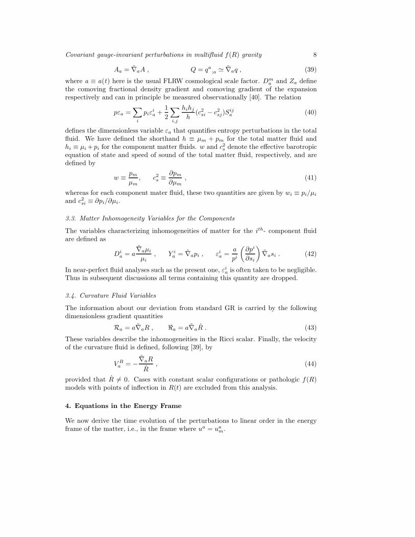
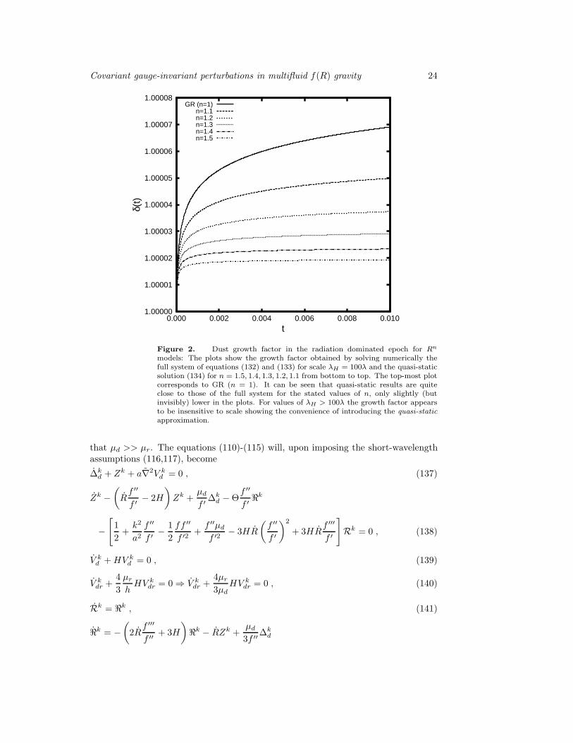
effect.In figure 2, we plot the normalized dust density contrast δ(t) ≡ ∆m(t)/∆eq in the

radiation-dominated epoch.

8.2. Perturbations in the Dust-dominated Epoch

During this epoch of the universe the dust energy density is dominating in the two-fluiddynamics and all order-of-magnitude approximations go in line with the assumption


1.00000

1.00001

1.00002

1.00003

1.00004

1.00005

1.00006

1.00007

1.00008

0.000 0.002 0.004 0.006 0.008 0.010

δ(t)

t

GR (n=1)n=1.1n=1.2n=1.3n=1.4n=1.5

Figure 2. Dust growth factor in the radiation dominated epoch for Rn

models: The plots show the growth factor obtained by solving numerically thefull system of equations (132) and (133) for scale λH = 100λ and the quasi-staticsolution (134) for n = 1.5, 1.4, 1.3, 1.2, 1.1 from bottom to top. The top-most plotcorresponds to GR (n = 1). It can be seen that quasi-static results are quiteclose to those of the full system for the stated values of n, only slightly (butinvisibly) lower in the plots. For values of λH > 100λ the growth factor appearsto be insensitive to scale showing the convenience of introducing the quasi-static

approximation.

that µd >> µr. The equations (110)-(115) will, upon imposing the short-wavelengthassumptions (116,117), become

∆kd + Zk + a∇2V k

d = 0 , (137)

Zk −(

Rf ′′

f ′ − 2H

)

Zk +µd

f ′ ∆kd −Θ

f ′′

f ′ ℜk

−[

1

2+

k2

a2f ′′

f ′ − 1

2

ff ′′

f ′2 +f ′′µd

f ′2 − 3HR

(

f ′′

f ′

)2

+ 3HRf ′′′

f ′

]

Rk = 0 , (138)

V kd +HV k

d = 0 , (139)

V kdr +

4

3

µr

hHV k

dr = 0 ⇒ V kdr +

4µr

3µd

HV kdr = 0 , (140)

Rk = ℜk , (141)

ℜk = −(

2Rf ′′′

f ′′ + 3H

)

ℜk − RZk +µd

3f ′′∆kd


−[

k2

a2+ (3HR+ R)

f ′′′

f ′′ + R2 f(iv)

f ′′ +f ′

3f ′′ −R

3

]

Rk . (142)

The resulting set of second order equations is therefore

∆kd +

(

2H − Rf ′′

f ′

)

∆kd − µd

f ′ ∆kd + 3H

f ′′

f ′ Rk

+

[

1

2+

k2

a2f ′′

f ′ − ff ′′

2f ′2 +f ′′µd

f ′2 − 3HR

(

f ′′

f ′

)2

+ 3HRf ′′′

f ′

]

Rk = 0 , (143)

Rk +

(

2Rf ′′′

f ′′ + 3H

)

Rk − R∆kd − µd

3f ′′∆kd

+

[

k2

a2+ (3HR+ R)

f ′′′

f ′′ + R2 f(iv)

f ′′ +f ′

3f ′′ −R

3

]

Rk = 0 . (144)

As can be observed, these two equations differ from their counterparts in the radiation-dominated epoch in that the curvature perturbations are not decoupled from that ofmatter in the system of equations.

The limiting GR perturbation equations for (143) and (144) in this epoch aregiven by

∆kd + 2H∆k

d − µd∆kd +

1

2Rk = 0 , (145)

− µd

3∆k

d +1

3Rk = 0 , (146)

and combine to give the equation

∆kd +

4

3t∆k

d −2

3t2∆k

d = 0 . (147)

This equation admits the well known solution

∆kd(t) = C1t

−1 + C2t23 . (148)

For Rn models, equations (143,144) take the form

∆kd +

(

10n− 6

3t

)

∆kd +

2(8n2 − 13n+ 3)

3t2∆k

d +3(n− 1)

2(4n− 3)tRk

+

[

n(n− 1)

3(4n− 3)

(

λH

λ

)2

eq

t2−4n3 +

27n2 − 8n3 − 18n

2n(4n− 3)

]

Rk = 0 , (149)

Rk +

{

8n [n(8n− 13) + 3] (4n− 3)

27(n− 1)t4

}

∆kd +

8n(4n− 3)

3t3∆k

d +8− 2n

tRk

+

{

4n2

9

(

λH

λ

)2

eq

t−4n3 − 2 [n(8n+ 5)− 69] + 54

9(n− 1)t2

}

Rk = 0 , (150)

where k2

a2 = 4n2

9

(

λH

λ

)2

eqt−

4n3 during this epoch.


Quasi-static Analysis In the quasi-static limit with(

λH

λ

)2

eq>> 1 we get a single

second order k-scale independent equation

∆kd +

4n

3t∆k

d +

[

4(8n2 − 13n+ 3)

9t2

]

∆kd = 0 , (151)

the solution of which is given by

∆kd(t) = C1t

α+ + C2tα− , (152)

where α± = − 2n3 + 1

2 ±√−112n2+184n−39

6 . The coefficients C1,2 can be determined byimposing initial conditions.

At t = teq = 1 we have

∆k(d) eq ≡ ∆k

(d)(teq) = C1 + C2 , (153)

and differentiating (152) gives

∆kd(t) = α+C1t

α+−1 + α−C2tα−−1 , (154)

which, at equality, will give

∆k(d) eq ≡ ∆k

(d)(teq) = α+C1 + α−C2 . (155)

Solving (153) and (155) simultaneously we obtain

C1,2 =±∆k

(d) eq ∓ α∓∆k(d) eq

α+ − α−. (156)

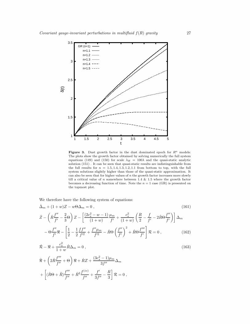
Fig. 3 shows the evolution of the density perturbations δ(t) ≡ ∆k(d)(t)/∆

k(d)eq in time

(t from 1 onwards, where t = teq = 1 is the normalized time at equality) for the abovelinearly independent solutions, C1,2 having been obtained by setting ∆k

(d)eq = 10−5

and ∆k(d)eq = 10−5 .

9. Long Wavelength Solutions

For specific intervals of n, a set of initial conditions give rise to cosmic histories whichinclude a transient decelerated phase which evolves towards an accelerated phase.Structure formation takes place during the transient regime [51].

In this section we analyze the evolution of scalar perturbations during thisphase, in the long wavelength limit. In this limit the wavenumber k is so small that

λ = 2πak

≫ λH , i.e., k2

a2H2 ≪ 1. All Laplacian terms can therefore be neglected and

spatially flat (K = 0) backgrounds guarantee the conservation of C, i.e., Ck = 0. Inthis paper we are considering only adiabatic perturbations, i.e. Sij = 0 and hence, fora radiation-dust mixture, the equation for the evolution of entropy perturbations

Sdr + a∇2Vdr = 0 . (157)

implies that

Vdr = 0 . (158)

And from this and the equation

Vdr −(

c2z −1

3

)

ΘVdr = − 1

ah(c2sd − c2sr)µ∆m − 1

ac2zSdr . (159)

follows

(c2sd − c2sr)µ∆m = 0 . (160)


1

1.5

2

2.5

3

3.5

1 1.5 2 2.5 3 3.5 4 4.5 5

δ(t)

t

GR (n=1)

n=1.1

n=1.2

n=1.3

n=1.4

n=1.5

Figure 3. Dust growth factor in the dust dominated epoch for Rn models:The plots show the growth factor obtained by solving numerically the full systemequations (149) and (150) for scale λH = 100λ and the quasi-static analyticsolution (151) . It can be seen that quasi-static results are indistinguishable fromthe full results for n = 1.5, 1.4, 1.3, 1.2, 1.1 from bottom to top, with the fullsystem solutions slightly higher than those of the quasi-static approximation. Itcan also be seen that for higher values of n the growth factor increases more slowlytill a critical value of n somewhere between 1.4 & 1.5 where the growth factorbecomes a decreasing function of time. Note the n = 1 case (GR) is presented onthe topmost plot.

We therefore have the following system of equations:

∆m + (1 + w)Z − wΘ∆m = 0 , (161)

Z −(

Rf ′′

f ′ − 2

3Θ

)

Z −[

(2c2s − w − 1)

(1 + w)

µm

f ′ +c2s

(1 + w)

(

R

2− f

f ′ − 2RΘf ′′

f ′

)]

∆m

−Θf ′′

f ′ ℜ −[

1

2− 1

2

ff ′′

f ′2 +f ′′µm

f ′2 − RΘ

(

f ′′

f ′

)2

+ RΘf ′′′

f ′

]

R = 0 , (162)

R − ℜ+c2s

1 + wR∆m = 0 , (163)

ℜ+

(

2Rf ′′′

f ′′ +Θ

)

ℜ+ RZ +(3c2s − 1)µm

3f ′′ ∆m

+

[

(RΘ+ R)f ′′′

f ′′ + R2 f(iv)

f ′′ +f ′

3f ′′ −R

3

]

R = 0 ,


C0

a2+

(

4

3Θ + 2

Rf ′′

f ′

)

Z − 2µm

f ′ ∆m +

[

2RΘf ′′′

f ′ − f ′′

f ′

(

f

f ′ − 2µm

f ′ + 2RΘf ′′

f ′

)]

R

+ 2Θf ′′

f ′ ℜ = 0, (164)

C0 being the conserved value for the quantity C.In terms of the background Rn solutions and making use of the conservation of

C the above equations can be rewritten as

∆m =

[

1 + w − 2n

1 + w− 6(n− 1)n

n+ 3(n− 1)w − 3

]

∆m

t

− 3(1 + w)2

4a20 [n+ 3(n− 1)w − 3] [4n− 3(1 + w)]t1−

4n3(1+w)C0

− 9(n− 1)(1 + w)3t2

4 [n+ 3(n− 1)w − 3] [4n− 3(1 + w)]t2ℜ

+

{

3(n− 1)(1 + w)2 [n(6w + 8)− 15(1 + w)]

4 [n+ 3(n− 1)w − 3] [4n− 3(1 + w)]

}

tR ,

(165)

R = ℜ+8nc2s [4n− 3(1 + w)]

3(1 + w)3∆m

t3, (166)

ℜ = −2

[

(n− 4) + 2(n− 2)w

(1 + w)t− 3n(n− 1)

n+ 3w(n− 1)− 3

]

ℜ

+2n(4n− 3w − 3)

(1 + w) [n+ 3(n− 1)w − 3]C0t

− 4n3(1+w)

−2

− 2

[

9n(n− 2)(n− 1)

n+ 3(n− 1)w − 3+ 2n2 − 7n− 3n2(9n− 26) + 57n

9(1 + w)(n − 1)− 8n2(n− 2)

9(1 + w)2(n− 1)

+6]Rt2

+ 16n∆m

t4[4n− 3(1 + w)] [4n+ 3(n− 1)w − 3]

27(n− 1)(1 + w)4 [n+ 3(n− 1)w − 3]×

[

(9w(1 + w) + 8)n2 −(

27w2 + 24w + 13)

n+ 3(1 + w)(1 + 6w)]

. (167)

9.1. Perturbations in the Radiation-dominated Epoch

The second order set of equations governing the dynamics of density perturbations inthis epoch is given by

∆kr +

n(9n− 14) + 4

2(n− 2)t∆k

r +n [n(n(19n− 54) + 58)− 32] + 8

2(n− 2)2t2∆k

r

+2 [n(3n− 4) + 2]

3(n− 2)2tRk − n(15n− 22) + 14

3(n− 2)Rk +

4(n2 − 1)

3(n− 2)2t−nC0 = 0, (168)

Rk − n(11n− 32) + 32

2(n− 2)tRk +

3 [n(5n− 9) + 8]

2t2Rk − 3n [n(n− 3) + 2]

2(n− 2)t3∆k

r


− 3n(n− 1) [n(19n− 28) + 4]

4(n− 2)t4∆k

r − 3n(n− 1)

(n− 2)t−(n+2)C0 = 0 . (169)

Making use of the conservation of C, we can eliminate Rk and Rk quantities in favourof ∆k

r (and its derivatives) and Co. This way we can get a decoupled third orderk-scale independent equation for ∆k

r :

d3

dt3∆k

r −n− 5

t

d2

dt2∆k

r +24n− 19n2 + 8

4t2d

dt∆k

r +(n− 2)

[

5n2 − 8n+ 2]

2t3∆k

r − (12− 7n)C0

3t(n+1)= 0 .

(170)

This equation admits the general solution

∆kr (t) = C1t

n

2 −1 + C2tβ+ + C3t

β− + C4t2−n . (171)

where C1,2,3 are arbitrary integration constants to be evaluated from initial conditionswith

C4 ≡ 2 (24− 14n)C0

9(7n3 − 18n2 + 16)(172)

and

β± ≡ −1

2+

n

4±√

3(81n2 − 44n+ 12)

4. (173)

Provided that the initial values of ∆kr , ∆

kr , ∆

kr and C0 are known at teq = 1, the

integration constants can be determined since

∆k(r)eq = C1 + C2 + C3 + C4,

∆k(r)eq =

(

n− 2

2

)

C1 + C2β+ + C3β− + (2− n)C4 ,

∆k(r)eq =

[

(n− 2)(n− 4)

4

]

C1 + C2β+(β+ − 1)

+ C3β−(β− − 1) + (2− n)(1 − n)C4 . (174)

We do not present C1,2,3 explicitly for the sake of simplicity.

9.2. Perturbations in the Dust-dominated Epoch

Proceeding in a similar fashion for the dust dominated, long wavelength, regime givesthe second order evolution equations given by

∆kd +

n(8n− 13) + 3

(n− 3)t∆k

d +[n(8n− 13) + 3] [n(16n− 15) + 9]

3(n− 3)2t2∆k

d

+3(n− 1) [n(16n− 15) + 9]

4(n− 3)2(4n− 3)tRk − n [(n(16n(8n− 31) + 711)− 540] + 189

4(n− 3)2(4n− 3)Rk

−n(

27 + 54n− 56n2)

− 27

4(n− 3)2(4n− 3)t−

4n3 C0 = 0 , (175)

Rk − 4(n− 1) [n(2n− 5) + 6]

[n(n− 4) + 3) tRk +

4 [n (n(2n(16n− 65) + 213)− 198) + 81]

9 [n(n− 4) + 3] t2Rk

− 16n(3− 4n)2 [n(8n− 13) + 3]

27 [(n− 4)n+ 3] t4∆k

d −2n [n(4n− 7) + 3]

n(n− 4) + 3t−(n+2)C0 = 0 , (176)


which reduce to a single third order evolution equation for the density perturbationsgiven as

d3

dt3∆k

d +5

t

d2

dt2∆k

d −2 [n (4n(8n− 19) + 33) + 9]

9(n− 1)t2d

dt∆k

d − 2(4n− 3) [n(8n− 13) + 3]

9(n− 1)t3∆k

d

−(

12n2 − 31n+ 18)

6(n− 1) tn+1C0 = 0 , (177)

which is a third order decoupled k-scale independent equation. The general solutionof (177) is given by

∆kd(t) = C1t

−1 + C2tγ+ + C3t

γ− + C4t2− 4n

3 , (178)

where C1,2,3 are arbitrary integration constants to be evaluated from initial conditionsand

C4 ≡9(

12n2 − 31n+ 18)

C0

8(48n4 − 184n3 + 159n2 + 63n− 81)(179)

together with

γ± ≡ −1

2∓ 1

6

√

256n3 − 608n2 + 417n− 81

n− 1. (180)

As in the radiation epoch, the integration constants C1,2,3 can be determined

from the initial values of ∆kd, ∆

kd, ∆

kd and C0 known at teq = 1 as follows:

∆k(d)eq = C1 + C2 + C3 + C4,

∆k(d)eq = −C1 + C2γ+ + C3γ− +

(

6− 4n

3

)

C4,

∆k(d)eq = 2C1 + C2γ+(γ+ − 1)

+ C3γ−(γ− − 1) +(6− 4n)(3− 4n)

9C4 . (181)

Once again, for the sake of simplicity, we do not present them here explicitly.It turns out that in the adiabatic limit, the long wavelength solutions of the

growth factor both in the radiation and dust epochs are exactly the same as thosefound in [51].

10. Conclusions

In this work we have for the first time presented a detailed analysis of the (1 + 3)-covariant and gauge-invariant theory of cosmological perturbations in situations wherethe universe is described by a multi-component fluid, with a general equation ofstate parameter for an arbitrary f(R) theory of gravity. The linearized evolutionequations of the density and curvature perturbations of such a universe have beenderived for both the fluid components and the total matter, relative to the energyframe. We then have taken the background transient solutions of Rn gravity for atwo-fluid system dominated respectively by radiation and CDM (dust) and obtainedsolutions in both the short and long wavelength approximations. These solutions areimportant when testing a full numerical implementation of these equations, importantfor generating the complete matter power spectrum for f(R) gravity theories with a


realistic background cosmological expansion history. We also found that for Rn gravityto be consistent with the Meszaros effect, the parameter n needs to satisfy n > 2/3.

We also gave a new covariant characterisation of the quasi-static approximationand used this to show that on small scales this approximation is valid for values of nin the neighbourhood of 1, i.e., it is in good agreement with a numerical integrationof the full set of equations for the given set of initial conditions. This is the first timesuch a quasi-static analysis has been presented in a covariant way both for radiationand dust universes and provided the foundations for detailed comparison with whatis found using the metric formalisms, together with a full computation of the powerspectra. This will be presented in a future work.

Acknowledgments

The authors thank the National Research Foundation (NRF-South Africa) for financialsupport. AdlCD also acknowledges nancial support from MICINN (Spain) projectnumbers FPA 2008-00592, FIS 2011-23000 and Consolider-Ingenio MULTIDARKCSD2009-00064.

References

[1] Moffat JW 2008 Reinventing Gravity, A Physicist goes beyond Einstein (NewYork:HarperCollins Publishers)

[2] Spergel DN et al 2003 ApJS 148 175-194[3] Frampton P 2005 (Preprint astro-ph/0506676 )[4] Copeland EJ, Sami M, Tsujikawa S 2006 Int. J. Mod. Phys. D 15 1753[5] Komatsu E et al 2011 ApJS 192 18[6] Bennett CL et al 2003 ApJS 148 97[7] Dobado A and Maroto AL 1995 Phys. Rev. D 52 1895[8] Dvali G, Gabadadze G and Porrati M 2000 Phys. Lett. B 485 208[9] Beltran J and Maroto AL 2008 Phys. Rev. D 78 063005 (2008); 2009 JCAP 0903 016 ; 2009

Phys. Rev. D 80 063512; 2009 Int. J. Mod. Phys. D 18 2243-2248[10] Sotiriou TP 2007 Modified Actions for Gravity: Theory and Phenomenology PhD thesis,

International School for Advanced Studies (SISSA), Trieste[11] Starobinsky AA 1980 Phys. Lett. 91B 99[12] Barrow JD and A. C. Ottewill AC 1983 J. Phys. A 16 2757[13] Nojiri S and Odintsov SD 2003 Phys. Rev. D 68 123512 ; 2004 Gen. Rel. Grav. 36 1765; 2007

Int. J. Geom. Meth. Mod. Phys. 4 115

[14] Carroll SM 2005 et al, Phys. Rev. D71 063513[15] Carloni S, Dunsby PKS, Capozziello S and Troisi A 2005 Class. Quant. Grav. 22 4839[16] Sotiriou TP and Faraoni V 2010 Rev. Mod. Phys. 82 451497[17] Faraoni V 2008 (Preprint arXiv:0810.2602v1 [gr-qc])[18] Weinberg S 1989 Rev. Mod. Phys 61 1[19] Ng YJ 1992 International Journal of Modern Physics D 1 145[20] Sotiriou TP and Liberati S 2007 Ann. Phys. 332 935-966[21] Cembranos JAR 2006 Phys. Rev. D 73 064029[22] Clifton T and Barrow JD 2005 Phys. Rev. D 72 103005[23] Capozziello S 2002 Int. J. Mod. Phys. D 11, 483; Capozziello S, Carloni S and Troisi A 2003

RecentRes.Dev.Astron.Astrophys.1:625 (Preprint arXiv: astro-ph/0303041)[24] Pogosian L and Silvestri A 2008 Phys. Rev. D 77 023503[25] Capozziello S and De Laurentis M 2011 (Preprint arXiv:1108.6266v2 [gr-qc])[26] Bardeen JM 1980 Phys. Rev. D 22 1882-1905[27] Kodama H and Sasaki M 1984 Progr.Theor.Phys. Suppl. 78 1[28] Brandenberger M, Kahn R, and Press WH 1983 Phys. Rev. D 28 1809-1821[29] Dodelson S 2003 Modern Cosmology (Amsterdam: Academic Press)[30] Padmanabhan T 1993 Structure formation in the Universe (Cambridge: Cambridge University

Press)

http://arxiv.org/abs/astro-ph/0506676

http://arxiv.org/abs/0810.2602


http://arxiv.org/abs/1108.6266


[31] Peebles PJE 1971 Physical Cosmology (Princeton: Princeton University Press)[32] Peebles PJE 1980 Large-scale structure of the Universe (Princeton: Princeton University Press)[33] Malik KA, Wands D 2009 Physics Reports 75, 1-4[34] Bertschinger E 2000 (Preprint arXiv:astro-ph/0101009)[35] Mukhanov VF, Feldman HA, Brandenberger RH 1992 Physics Reports. 215 203-333[36] Bernardis 2000 P et al, Nature 404 955-959[37] Ellis GFR and Bruni M 1989 Phys. Rev. D 40 1804[38] Dunsby PKS, Bruni M and Ellis GFR 1992 Astrophys. J. 395 54[39] Bruni M, Ellis GFR, and Dunsby PKS 1992 Class. Quantum Grav. Grav. 9 921-945[40] Bruni M, Dunsby PKS and Ellis GFR 1992 Ap. J. 395 34[41] Dunsby PKS 1991 Class. Quantum Grav. 8 1785[42] Carroll SM, Sawicki I, Silvestri A and Trodden M 2006 New J. Phys. 8 323 Tsujikawa S 2008

Phys. Rev. D 77 023507 Pogosian L and Silvestri A 2008 Phys. Rev. D 77 023503 StarobinskyAA 2007 JETP Lett. 86 157

[43] Bean R, Bernat D, Pogosian L, Silvestri A and Trodden M 2007 Phys. Rev. D 75 064020[44] Ananda KN, Carloni S and Dunsby PKS 2009 Class. Quant. Grav. 26 235018[45] Hwang J 1990 Phys. Rev. D 42 2601[46] Dunsby PKS 1992 Perturbations in general relativity and cosmology PhD thesis, Queen Mary

and Westfield College, London[47] Sotiriou TP 2006 Gen. Rel. Grav. 38 1407 Mena O, Santiago J and Weller J 2006 Phys. Rev.

Lett. 96 041103 Faraoni V 2006 Phys. Rev. D 74 023529 Cruz-Dombriz Adl and DobadoA 2006 Phys. Rev. D 74 087501 Nojiri S and Odintsov SD 2006 Phys. Rev. D 74 086005Sawicki I and Hu W 2007 Phys. Rev. D 75 127502.

[48] Cruz-Dombriz Adl, Dobado A and Maroto AL 2008 Phys. Rev. D 77 123515[49] Cruz-Dombriz Adl, Dobado A and Maroto AL 2009 Phys. Rev. Lett. 103 179001[50] G. F. R. Ellis, M. Bruni, and J. Hwang 1990 Phys. Rev. D 42 1035[51] Carloni S, Dunsby PKS and Troisi A 2008 Phys. Rev. D 77 024024[52] King AR and Ellis GFR 1973 Com. Math. Phys. 31, 209[53] Meszaros P 1974 Astron & Astrophys. 37 225-228


Documents

Covariant gauge-invariant perturbations in multifluid f(R) gravity