Crustal shear velocity structure of the south Indian shield

Crustal shear velocity structure of the south Indian shield

S. S. Rai,1 Keith Priestley,2 K. Suryaprakasam,1 D. Srinagesh,1 V. K. Gaur,3,4 and Z. Du5

Received 21 January 2002; revised 2 August 2002; accepted 30 October 2002; published 11 February 2003.

[1] The south Indian shield is a collage of Precambrian terrains gathered around and inpart derived from the Archean-age Dharwar craton. We operated seven broadbandseismographs on the shield along a N-S corridor from Nanded (NND) to Bangalore (BGL)and used data from these to determine the seismic characteristics of this part of the shield.Surface wave dispersion and receiver function data from these sites and the Geoscopestation at Hyderabad (HYB) give the shear wave velocity structure of the crust along this600 km long transect. Inversion of Rayleigh wave phase velocity measured along theprofile shows that the crust has an average thickness of 35 km and consists of a 3.66 kms�1, 12 km thick layer overlying a 3.81 km s�1, 23 km thick lower crust. At all sites,the receiver functions are extremely simple, indicating that the crust beneath each site isalso simple with no significant intracrustal discontinuities. Joint inversion of thereceiver function and surface wave phase velocity data shows the seismic characteristics ofthis part of the Dharwar crust to be remarkably uniform throughout and that it varieswithin fairly narrow bounds: crustal thickness (35 ± 2 km), average shear wave speed(3.79 ± 0.09 km s�1), and Vp/Vs ratio (1.746 ± 0.014). There is no evidence for a highvelocity basal layer in the receiver function crustal images of the central Dharwar craton,suggesting that there is no seismically distinct layer of mafic cumulates overlying theMoho and implying that the base of the Dharwar crust has remained fairly refractory sinceits cratonization. INDEX TERMS: 7203 Seismology: Body wave propagation; 7205 Seismology:

Continental crust (1242); 7255 Seismology: Surface waves and free oscillations; KEYWORDS: continental

crust, Archean crust, receiver function, Indian shield

Citation: Rai, S. S., K. Priestley, K. Suryaprakasam, D. Srinagesh, V. K. Gaur, and Z. Du, Crustal shear velocity structure of the

south Indian shield, J. Geophys. Res., 108(B2), 2088, doi:10.1029/2002JB001776, 2003.

1. Introduction

[2] Precambrian shields and platforms account for �70%of the continental crust. The seismic characteristics of theseregions provide insightful clues for discriminating betweenvarious contending hypotheses of crustal growth, whetherby steady state or by evolutionary processes governed bythe thermal history of the mantle. Three specific crustalseismic parameters provide strong constraints to be imposedon models of crustal evolution: (1) the thickness of thecrust; that is, depth to the seismic Mohorovicic disconti-nuity, (2) the presence or absence of a basal cumulate layerin which the shear velocity increases from about 4.0 to 4.35km s�1 and, if present, its thickness, and (3) the Poisson’sratio s or Vp/Vs of the crust. Knowledge of the lateralvariation of these three properties provides critical input for

modeling seismic wave propagation in the crustal wave-guide, which has strong influence on quantification ofregional seismic hazards and of the source characteristicsof earthquakes.[3] In this study, we discuss the results of an experiment

designed to determine the shear velocity structure andthickness of the crust beneath a 600 km long N-S transectof the relatively poorly studied south Indian shield, acollage of Precambrian terrains gathered around and in partderived from the Archean-age Dharwar craton (Figure 1). Alarge expanse of the northern Dharwar craton lies buriedbeneath the cover of Deccan flood basalts (65 Ma); else-where, the south Indian shield is dominated by the ubiq-uitous Peninsular Gneisses (3.3–2.6 Ga) that surround andseparate the shield’s variegated components, including someof its oldest relics (3.6 Ga) of migmatitic and gneissic rocks.The Closepet granite, which evolved by anatexis of its host,divides the Dharwar craton longitudinally. To the south, therocks of the south Indian shield pass through a narrowgradational zone and into the high-grade granulites of lateArchean metamorphism (2.6 Ga). Further south, across theNoyil-Kaveri shear zone (Figure 1), the high-grade gran-ulites are joined to the metamorphic terrains of Pan Africanorogeny. The latter cover the entire southern peninsula,alternately exposing a migmatitic complex and the granulitemassifs of Palni, Kodaikanal, and Periyakulum as well as

JOURNAL OF GEOPHYSICAL RESEARCH, VOL. 108, NO. B2, 2088, doi:10.1029/2002JB001776, 2003

1National Geophysical Research Institute, Hyderabad, India.2Bullard Laboratories, University of Cambridge, Cambridge, United

Kingdom.3Centre for Mathematical Modeling and Computer Simulation,

Bangalore, India.4Indian Institute of Astrophysics, Bangalore, India.5Institute of Theoretical Geophysics, University of Cambridge, Cam-

bridge, United Kingdom.

Copyright 2003 by the American Geophysical Union.0148-0227/03/2002JB001776$09.00

ESE 10 - 1

intrusives, of which the Proterozoic alkaline complex ofSivamalai is the most prominent.[4] Little research has been done on the seismic struc-

ture of the south Indian shield. Dube et al. [1973]analyzed travel times of crustal phases from aftershocksof the 1967 mb 6.7 Koyna earthquake and inferred fromthese a two-layer crust consisting of a 20 km thick graniticlayer (Vp 5.78 km s�1, Vs 3.42 km s�1), a 18.7 km thickbasaltic lower crust (Vp 6.58 km s�1, Vs 3.92 km s�1) anda Pn and Sn velocity of 8.19 and 4.62 km s�1, respectively.Our transect, which will be discussed below, is crossedabout midway by the 600 km long ENE-WSW refractionseismic profile [Kaila and Krishna, 1992] from Kavali onthe east coast to Uduppi on the west coast (Figure 1).These refraction data show an upper crust with P wavevelocity of 6.4 km s�1, a Moho depth varying from 34 kmin the east to 41 km in the west, and high Pn velocities of8.4–8.6 km s�1.[5] Crustal structure in the vicinity of Gauribidnaur

(GBA) (Figure 1) near the southern end of our transect isdiscussed by Krishna and Ramesh [2000] who inverted theseismic wave field from mine tremors and explosionsrecorded on the GBA short period vertical seismograph

array. They interpreted the group velocity and coda lengthsof the seismograms as indicating a laminated upper crustalwaveguide at 5–15 km depth. They find the Moho depthbeneath GBA to be 34–36 km, the Pn velocity to be 8.2 kms�1, and a value of 0.24 (Vp/Vs = 1.71) for the Poisson’sratio just below the Moho. Krishna et al. [1999] analyzedtravel times and waveforms of aftershocks of the Laturearthquake to determine a 1-D, P and S wave crustal modelnear KIL (Figure 1). Their model contains alternating lowvelocity layers (�7% velocity reduction) for both P and Swaves in the upper crust at depths between 6.5–9.0 and12.3–14.5 km and a lower crustal low velocity layer at 24–26 km depth. The arrival times of SmS phases (the S wavereflection from the Moho) indicated a Moho depth of 35–37km, while the Poisson’s ratio was found to be 0.21 (Vp/Vs =1.65) for the upper crust and 0.226 (Vp/Vs = 1.68) for thelower crust.[6] Little is known about the S wave structure of the south

Indian shield. Gaur and Priestley [1997] used receiverfunction analysis of 11 events with the highest signal-to-noise ratio occurring in two compact clusters during theperiod 1989–1996 to determine the shear wave structure ofthe crust beneath the Geoscope station at Hyderabad (HYB)(Figure 1). Their study showed that the crust beneath theHYB granites is quite simple, possesses a thickness of 36 ±1 km, and consists of a 10 km thick upper layer in which theshear velocity is 3.54 ± 0.07 km s�1 underlain by a 26 ± 1km thick lower crust in which the shear wave velocity variesuniformly with a small gradient of 0.02 s�1. The shear wavevelocity at the base is 4.1 ± 0.1 km s�1 just above the Mohotransition zone, which is constrained to be less than 4 kmthick and overlies a 4.74 ± 0.1 km s�1 half-space. Saul et al.[2000] used a data set of 297 events recorded at HYB andconfirmed these basic findings: a seismically transparentcrust beneath HYB and a shallow Moho (33 ± 2 km). Zhouet al. [2000] also analyzed HYB broadband data from 38events by constraining the shear wave velocity in the crustfrom a joint analysis of receiver function and Rayleigh wavedispersion measured over a broad region of India by Hwangand Mitchell [1987] and Bhattacharya [1992]. Their anal-ysis also indicates a low average shear velocity for the HYBcrust (3.58 ± 0.01 km s�1), a shallow Moho (32 ± 2 km),and a Poisson’s ratio of 0.26 ± 0.01. Singh et al. [1999]measured group velocity dispersion from seismograms ofthe 1997 Jabalpur earthquake at several stations on theIndian shield. Inversion of the group velocity data gave anaverage crustal model consisting of a two-layer crust (H1

13.8 km, Vp1 5.68 km s�1, Vs1 3.55 km s�1; H2 24.9 km, Vp2

6.16 km s�1, Vs2 3.85 km s�1) overlying an upper mantlewith Vpn 8.01 km s�1 and Vsn 4.65 km s�1. Kumar et al.[2001] find a crustal thickness of 36.5 km, average shearvelocity of 3.7 km s�1 and Poisson’s ratio of 0.26 at twosites on the Deccan basalt flows to the west of HYB. Atthese sites, the Deccan basalts are likely to form a thinveneer overlying rocks of the west Dharwar craton.

2. Data and Methodology

[7] In this study we examine the crustal shear wavestructure of the south Indian shield along a 600 km longN-S transect from Nanded (NND) in the north to Bangalore(BGL) in the south (Figure 1). This transect lies along the

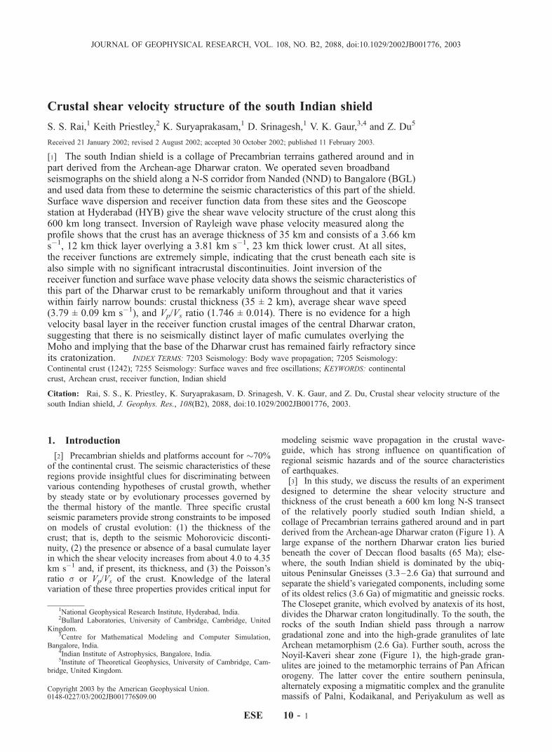
Figure 1. Principle geologic units of the south Indianshield. The seven sites with broadband seismographsoperated by NGRI and the Indian Institute of Astrophysics,jointly with the University of Cambridge, are designated bysolid triangles. The location of the Geoscope station atHyderabad is denoted by the solid square.

ESE 10 - 2 RAI ET AL.: SOUTH INDIAN SHIELD CRUSTAL STRUCTURE

western boundary of the eastern Dharwar craton andapproximately parallels the Closepet granitic intrusion. Wedeployed seven broadband digital seismographs (Figure 1)along this profile and operated these stations for about 15–18 months. Stations BGL, GBA, LTV, and MNB all lie onArchean crystalline outcrops of the Dharwar craton; KILand NND lie on a thin veneer of Deccan basalt flow (�350m) below which lie rocks of the Dharwar craton; and SLMis situated on the northeastern part of the Cuddappah Basin.Seismograms from these seven sites and from the Geoscopestation at HYB (Figure 1) provide the data for our study. Weanalyze teleseismic receiver functions and surface wavephase velocity from these data to constrain the averagecrustal shear wave velocity, the Moho depth, the Vp/Vs ratioof the crust, the velocity gradient in the crust–mantletransition zone and Moho sharpness beneath this part ofthe south Indian shield.

2.1. Surface Wave Dispersion Analysis

[8] Crustal structure has previously been determined atthree points along the NND–BGL transect (Figure 1): nearKIL [Krishna et al., 1999], near GBA [Krishna andRamesh, 2000], and between GBA and LTV [Kaila andKrishna, 1992]. All show a similar crustal thickness of �35km but indicate a possible small increase in average P wavespeed for the crust from �6.4 km s�1 in the south to �6.5km s�1 in the north. We first measure the short period (15–35 s) fundamental mode Rayleigh wave phase velocity andinvert these dispersion data to determine the average shearwave velocity of the crust beneath the transect.[9] We measure two-station fundamental mode Rayleigh

wave phase velocity from eleven events nearly alignedalong the same great circle path (<10�) as station pairs(Table 1), using the transfer function method of Gomberg etal. [1988]. This method poses the problem of phase velocitydetermination as a linear filter estimation problem in whichthe seismogram at a more distant station from an event isconsidered the convolution of the seismogram at a closestation with the Earth filter (the dispersion curve), which isto be determined. Smoothness constraints are imposedbased on an approximate knowledge of the group velocity.We used the results of Bhattacharya [1992] as an initialdispersion model. To ensure that the starting dispersioncurve was appropriate, we tested a number of variations

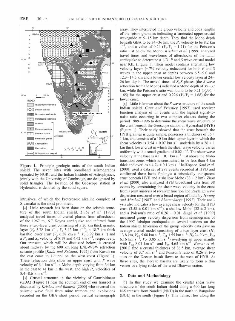
of the initial dispersion models and smoothing criteria. Wedetermined dispersion curves for the full length of thetransect and, separately, curves for the northern (KIL–SLM) and southern (SLM–BGL) halves of the transect.We inverted the dispersion along the transect to provide anaverage crustal model which could be used as the startingmodel for the receiver function inversion; we used thedispersion measured for the halves of the profile in thejoint receiver function–phase velocity inversion. The dis-persion curves were determined simultaneously from multi-ple station pairs, but we also calculated dispersion curvesfor all individual two-station paths separately to verify thatthere were no large outliers among the various two-stationcombinations.[10] We invert the Rayleigh wave phase velocity meas-

ured along the full transect using the stochastic least squaresroutine of Hermann [1994]. This expresses the least squaresproblem in terms of eigenvalues and eigenvectors and usessingular value decomposition to invert the matrix giving thesolution vector, the variance–covariance matrix, and theresolution matrix. The starting model for the inversion isfrom the average crustal model for the Indian shield ofSingh et al. [1999] and the 4.72 km s�1Sn velocity measure-ment of Huestis et al. [1973]. The starting model has beenparameterized in terms of 2 km thick layers over a half-space upper mantle. After the initial inversion, adjacent thinlayers with nearly the same velocities were grouped intothicker layers, resulting in a coarser model; we repeat theinversion to find the minimum number of crustal parameterswhich explain the observed dispersion. The final inversionmodel (Figure 2b) and the fit of the dispersion curve for thismodel to the observed dispersion (Figure 2a) show that theaverage crustal structure beneath the profile consists of twolayers: an upper 12 km thick layer with Vs 3.65 km s�1, anda lower 23 km thick layer with Vs 3.81 km s�1, overlying anupper mantle with Sn velocity 4.61 km s�1.

2.2. Receiver Function Analysis

[11] The teleseismic P wave coda contains S wavesgenerated by P-to-S conversions at significant velocitycontrasts in the crust and upper mantle below the seismo-graph site. Receiver functions are radial and transversewaveforms created by deconvolving the vertical componentfrom the radial and transverse components of the seismo-gram to isolate the receiver site effects from the other

Table 1. Surface Wave Analysis Summary

Date Origin Time (UTC) Latitude (�N) Longitude (�E) Full Profile North Section South Section

1999/01/16 1044:39.4 56.2 �147.4 NND–KIL (9.0)a SLM–GBA (6.5)SLM–BGL (1.0)

1999/01/24 0037:04.6 30.6 131.1 SLM–LTV (9.5)1999/01/24 0800:08.5 �26.5 74.5 HYB–BGL (7.0)1999/01/28 0810:05.4 52.9 �169.1 NND–KIL (1.0) SLM–GBA (3.5)1999/02/01 1635:31.1 �6.5 104.7 SLM–KIL (2.5)1999/02/03 0635:56.6 �6.2 104.2 SLM–KIL (2.0)1999/03/20 1047:45.9 51.6 �177.7 SLM–GBA (6.5)1999/03/21 1616:02.2 55.9 110.2 NND–KIL (6.0) SLM–GBA (6.5)1999/03/28 1905:11.0 30.5 79.4 BGL–NND (8.5)

GBA–LTV (10.0)GBA–NND (7.5)

1999/08/01 1247:50.1 51.5 �176.3 NND–KIL (4.5)1999/12/29 0519:46.9 18.2 �101.4 NND–MBN (7.5) LTV–BGL (6.5)

aNumbers in brackets following the two station pairs used for the interstation phase velocity measurement denote the difference in azimuth between thegreat circle path joining the stations and the great circle path joining the stations and the epicenter.

RAI ET AL.: SOUTH INDIAN SHIELD CRUSTAL STRUCTURE ESE 10 - 3

information contained in a teleseismic P wave. The use ofreceiver functions to determine crust and upper mantlevelocity structure beneath three-component broadband seis-mographs is now a well-established seismological techni-que; various approaches for interpreting receiver functionshave been discussed in the literature [Owens et al., 1984;Priestley et al., 1988; Zandt et al., 1995; Sheehan et al.,1995; Zhu and Kanamori, 2000]. We follow the procedureof Ammon et al. [1990] and compute true amplitude radialand tangential receiver functions [Ammon, 1991] and low-pass filter these at 1.2 Hz. The resulting receiver functionsconsist of wavelengths greater than 5–6 km; therefore, theminimum resolvable model layer thickness is approximately2–3 km.[12] Those receiver functions whose averaging functions

[Ammon, 1991] resembled a narrow Gaussian pulse andwhich emanated in a limited back azimuth and epicentraldistance range were stacked, and the ±1 standard deviation(s) bounds calculated. These bounds were used to evaluatehow well particular phases of the waveform are determined.We obtain a shear wave crustal model using the linearizedinversion procedure of Ammon et al. [1990] as modified toinclude the joint surface wave phase velocity constraint [Duand Foulger, 1999]. A starting model is parameterized as astack of thin horizontal layers to a depth of 60 km. The Swave velocity is the free parameter in the inversion, the Pwave velocity is set assuming a Poisson’s ratio of 0.25 andthe layer thicknesses are fixed. The radial receiver functionis inverted by minimizing the difference between theobserved receiver function and synthetic receiver functionscomputed from the model, while simultaneously constrain-ing the model smoothness.[13] We illustrate the details of our analysis procedure

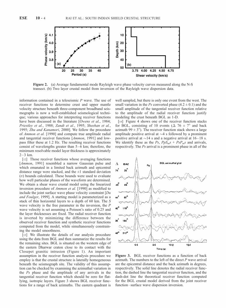
using the data from BGL and then summarize the results forthe remaining sites. BGL is situated on the western edge ofthe eastern Dharwar craton close to its contact with theClosepet granitic intrusion (Figure 1). An importantassumption in the receiver function analysis procedure weemploy is that the crustal structure is laterally homogeneousbeneath the seismograph site. The validity of this assump-tion can be checked by examining the azimuthal variation inthe Ps phase and the amplitude of any arrivals in thetangential receiver function which should be zero for flat-lying, isotropic layers. Figure 3 shows BGL receiver func-tions for a range of back azimuths. The eastern quadrant is

well sampled, but there is only one event from the west. Thesmall variation in the Ps converted phase (4.2 ± 0.1) and thesmall amplitude of the tangential receiver function relativeto the amplitude of the radial receiver function justifymodeling the crust beneath BGL as 1-D.[14] Figure 4 shows one of the receiver function stacks

for BGL, consisting of 10 events (� 76 ± 7� and backazimuth 99 ± 3�). The receiver function stack shows a largeamplitude positive arrival at �4 s followed by a prominentpositive arrival at �14 s and a negative arrival at 16–18 s.We identify these as the Ps, PpSms + PsPms and arrivals,respectively. The Ps arrival is a prominent phase in all of the

Figure 2. (a) Average fundamental mode Rayleigh wave phase velocity curves measured along the N-Stransect. (b) Two layer crustal model from inversion of the Rayleigh wave dispersion data.

Figure 3. BGL receiver functions as a function of backazimuth. The numbers to the left of the direct P wave arrivalare the epicentral distance and the back azimuth in degrees,respectively. The solid line denotes the radial receiver func-tion, the dashed line the tangential receiver function, and thedash-dot line the theoretical receiver function computedfor the BGL crustal model derived from the joint receiverfunction–surface wave dispersion inversion.


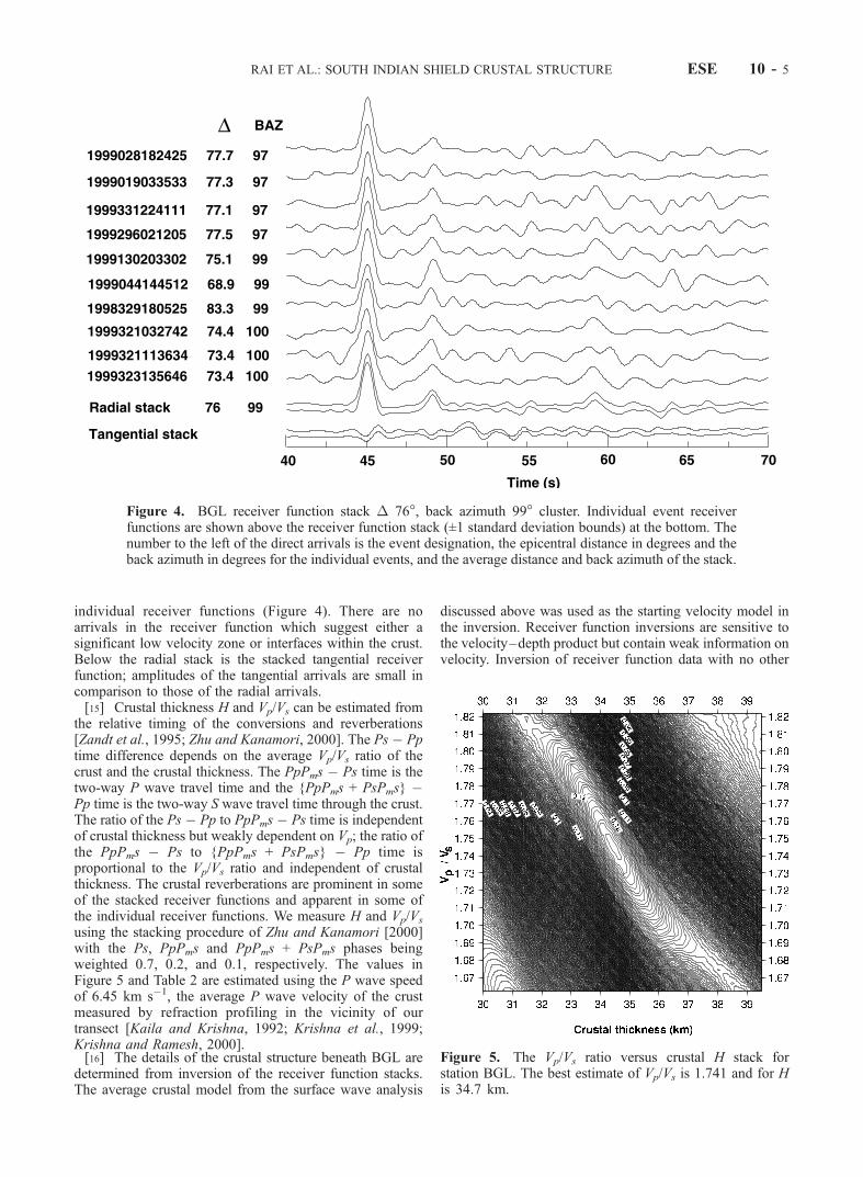
individual receiver functions (Figure 4). There are noarrivals in the receiver function which suggest either asignificant low velocity zone or interfaces within the crust.Below the radial stack is the stacked tangential receiverfunction; amplitudes of the tangential arrivals are small incomparison to those of the radial arrivals.[15] Crustal thickness H and Vp/Vs can be estimated from

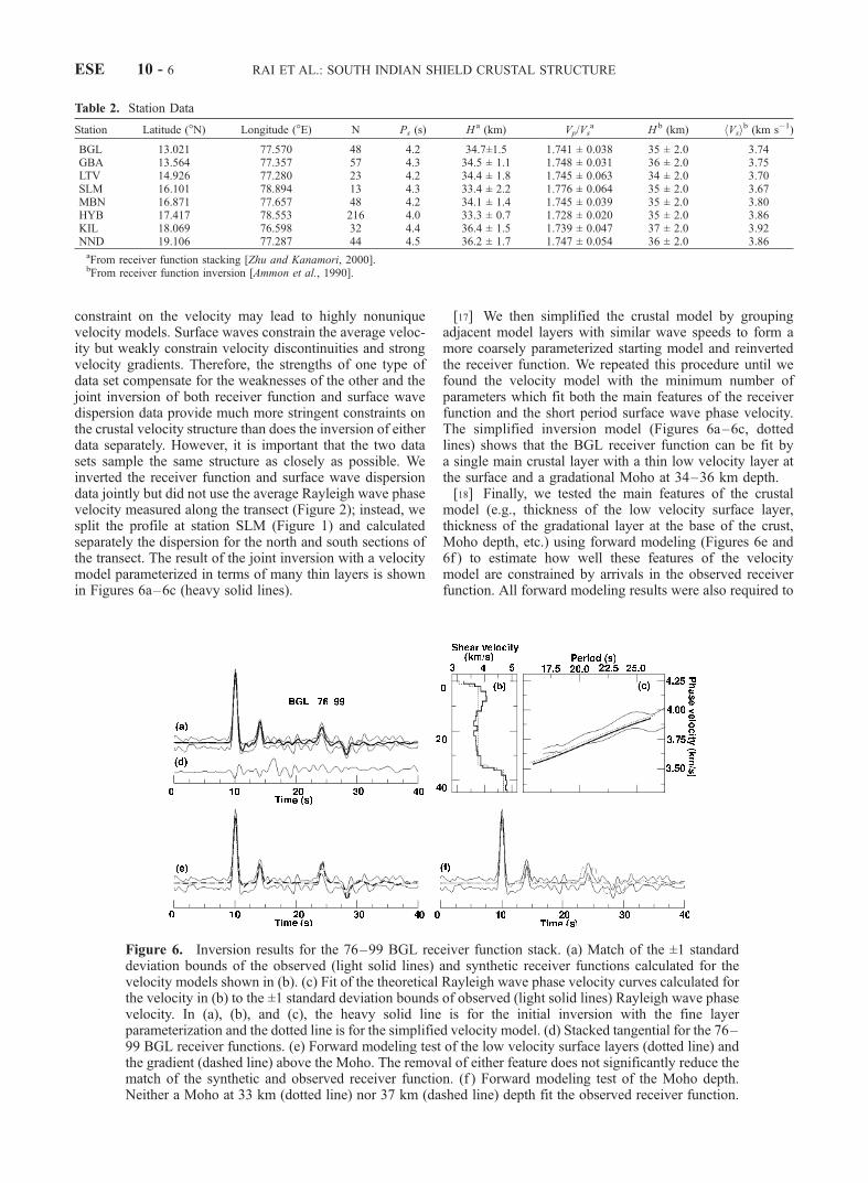
the relative timing of the conversions and reverberations[Zandt et al., 1995; Zhu and Kanamori, 2000]. The Ps � Pptime difference depends on the average Vp/Vs ratio of thecrust and the crustal thickness. The PpPms � Ps time is thetwo-way P wave travel time and the {PpPms + PsPms} �Pp time is the two-way S wave travel time through the crust.The ratio of the Ps � Pp to PpPms � Ps time is independentof crustal thickness but weakly dependent on Vp; the ratio ofthe PpPms � Ps to {PpPms + PsPms} � Pp time isproportional to the Vp/Vs ratio and independent of crustalthickness. The crustal reverberations are prominent in someof the stacked receiver functions and apparent in some ofthe individual receiver functions. We measure H and Vp/Vs

using the stacking procedure of Zhu and Kanamori [2000]with the Ps, PpPms and PpPms + PsPms phases beingweighted 0.7, 0.2, and 0.1, respectively. The values inFigure 5 and Table 2 are estimated using the P wave speedof 6.45 km s�1, the average P wave velocity of the crustmeasured by refraction profiling in the vicinity of ourtransect [Kaila and Krishna, 1992; Krishna et al., 1999;Krishna and Ramesh, 2000].[16] The details of the crustal structure beneath BGL are

determined from inversion of the receiver function stacks.The average crustal model from the surface wave analysis

discussed above was used as the starting velocity model inthe inversion. Receiver function inversions are sensitive tothe velocity–depth product but contain weak information onvelocity. Inversion of receiver function data with no other

Figure 4. BGL receiver function stack � 76�, back azimuth 99� cluster. Individual event receiverfunctions are shown above the receiver function stack (±1 standard deviation bounds) at the bottom. Thenumber to the left of the direct arrivals is the event designation, the epicentral distance in degrees and theback azimuth in degrees for the individual events, and the average distance and back azimuth of the stack.

Figure 5. The Vp/Vs ratio versus crustal H stack forstation BGL. The best estimate of Vp/Vs is 1.741 and for His 34.7 km.


constraint on the velocity may lead to highly nonuniquevelocity models. Surface waves constrain the average veloc-ity but weakly constrain velocity discontinuities and strongvelocity gradients. Therefore, the strengths of one type ofdata set compensate for the weaknesses of the other and thejoint inversion of both receiver function and surface wavedispersion data provide much more stringent constraints onthe crustal velocity structure than does the inversion of eitherdata separately. However, it is important that the two datasets sample the same structure as closely as possible. Weinverted the receiver function and surface wave dispersiondata jointly but did not use the average Rayleigh wave phasevelocity measured along the transect (Figure 2); instead, wesplit the profile at station SLM (Figure 1) and calculatedseparately the dispersion for the north and south sections ofthe transect. The result of the joint inversion with a velocitymodel parameterized in terms of many thin layers is shownin Figures 6a–6c (heavy solid lines).

[17] We then simplified the crustal model by groupingadjacent model layers with similar wave speeds to form amore coarsely parameterized starting model and reinvertedthe receiver function. We repeated this procedure until wefound the velocity model with the minimum number ofparameters which fit both the main features of the receiverfunction and the short period surface wave phase velocity.The simplified inversion model (Figures 6a–6c, dottedlines) shows that the BGL receiver function can be fit bya single main crustal layer with a thin low velocity layer atthe surface and a gradational Moho at 34–36 km depth.[18] Finally, we tested the main features of the crustal

model (e.g., thickness of the low velocity surface layer,thickness of the gradational layer at the base of the crust,Moho depth, etc.) using forward modeling (Figures 6e and6f ) to estimate how well these features of the velocitymodel are constrained by arrivals in the observed receiverfunction. All forward modeling results were also required to

Table 2. Station Data

Station Latitude (�N) Longitude (�E) N Ps (s) H a (km) Vp/Vsa H b (km) hVsib (km s�1)

BGL 13.021 77.570 48 4.2 34.7±1.5 1.741 ± 0.038 35 ± 2.0 3.74GBA 13.564 77.357 57 4.3 34.5 ± 1.1 1.748 ± 0.031 36 ± 2.0 3.75LTV 14.926 77.280 23 4.2 34.4 ± 1.8 1.745 ± 0.063 34 ± 2.0 3.70SLM 16.101 78.894 13 4.3 33.4 ± 2.2 1.776 ± 0.064 35 ± 2.0 3.67MBN 16.871 77.657 48 4.2 34.1 ± 1.4 1.745 ± 0.039 35 ± 2.0 3.80HYB 17.417 78.553 216 4.0 33.3 ± 0.7 1.728 ± 0.020 35 ± 2.0 3.86KIL 18.069 76.598 32 4.4 36.4 ± 1.5 1.739 ± 0.047 37 ± 2.0 3.92NND 19.106 77.287 44 4.5 36.2 ± 1.7 1.747 ± 0.054 36 ± 2.0 3.86aFrom receiver function stacking [Zhu and Kanamori, 2000].bFrom receiver function inversion [Ammon et al., 1990].

Figure 6. Inversion results for the 76–99 BGL receiver function stack. (a) Match of the ±1 standarddeviation bounds of the observed (light solid lines) and synthetic receiver functions calculated for thevelocity models shown in (b). (c) Fit of the theoretical Rayleigh wave phase velocity curves calculated forthe velocity in (b) to the ±1 standard deviation bounds of observed (light solid lines) Rayleigh wave phasevelocity. In (a), (b), and (c), the heavy solid line is for the initial inversion with the fine layerparameterization and the dotted line is for the simplified velocity model. (d) Stacked tangential for the 76–99 BGL receiver functions. (e) Forward modeling test of the low velocity surface layers (dotted line) andthe gradient (dashed line) above the Moho. The removal of either feature does not significantly reduce thematch of the synthetic and observed receiver function. (f ) Forward modeling test of the Moho depth.Neither a Moho at 33 km (dotted line) nor 37 km (dashed line) depth fit the observed receiver function.


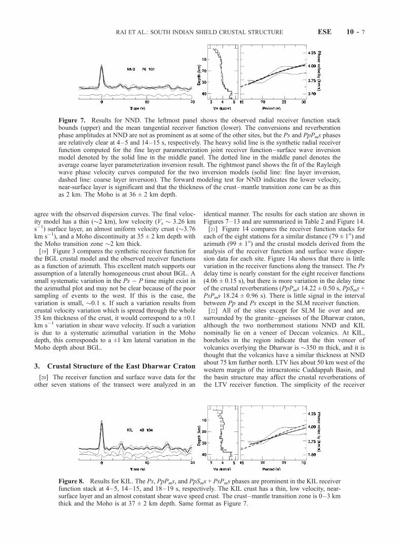
agree with the observed dispersion curves. The final veloc-ity model has a thin (�2 km), low velocity (Vs � 3.26 kms�1) surface layer, an almost uniform velocity crust (�3.76km s�1), and a Moho discontinuity at 35 ± 2 km depth withthe Moho transition zone �2 km thick.[19] Figure 3 compares the synthetic receiver function for

the BGL crustal model and the observed receiver functionsas a function of azimuth. This excellent match supports ourassumption of a laterally homogeneous crust about BGL. Asmall systematic variation in the Ps � P time might exist inthe azimuthal plot and may not be clear because of the poorsampling of events to the west. If this is the case, thevariation is small, �0.1 s. If such a variation results fromcrustal velocity variation which is spread through the whole35 km thickness of the crust, it would correspond to a ±0.1km s�1 variation in shear wave velocity. If such a variationis due to a systematic azimuthal variation in the Mohodepth, this corresponds to a ±1 km lateral variation in theMoho depth about BGL.

3. Crustal Structure of the East Dharwar Craton

[20] The receiver function and surface wave data for theother seven stations of the transect were analyzed in an

identical manner. The results for each station are shown inFigures 7–13 and are summarized in Table 2 and Figure 14.[21] Figure 14 compares the receiver function stacks for

each of the eight stations for a similar distance (79 ± 1�) andazimuth (99 ± 1�) and the crustal models derived from theanalysis of the receiver function and surface wave disper-sion data for each site. Figure 14a shows that there is littlevariation in the receiver functions along the transect. The Psdelay time is nearly constant for the eight receiver functions(4.06 ± 0.15 s), but there is more variation in the delay timeof the crustal reverberations (PpPms 14.22 ± 0.50 s, PpSms +PsPms 18.24 ± 0.96 s). There is little signal in the intervalbetween Pp and Ps except in the SLM receiver function.[22] All of the sites except for SLM lie over and are

surrounded by the granite–gneisses of the Dharwar craton,although the two northernmost stations NND and KILnominally lie on a veneer of Deccan volcanics. At KIL,boreholes in the region indicate that the thin veneer ofvolcanics overlying the Dharwar is �350 m thick, and it isthought that the volcanics have a similar thickness at NNDabout 75 km further north. LTV lies about 50 km west of thewestern margin of the intracratonic Cuddappah Basin, andthe basin structure may affect the crustal reverberations ofthe LTV receiver function. The simplicity of the receiver

Figure 7. Results for NND. The leftmost panel shows the observed radial receiver function stackbounds (upper) and the mean tangential receiver function (lower). The conversions and reverberationphase amplitudes at NND are not as prominent as at some of the other sites, but the Ps and PpPms phasesare relatively clear at 4–5 and 14–15 s, respectively. The heavy solid line is the synthetic radial receiverfunction computed for the fine layer parameterization joint receiver function–surface wave inversionmodel denoted by the solid line in the middle panel. The dotted line in the middle panel denotes theaverage coarse layer parameterization inversion result. The rightmost panel shows the fit of the Rayleighwave phase velocity curves computed for the two inversion models (solid line: fine layer inversion,dashed line: coarse layer inversion). The forward modeling test for NND indicates the lower velocity,near-surface layer is significant and that the thickness of the crust–mantle transition zone can be as thinas 2 km. The Moho is at 36 ± 2 km depth.

Figure 8. Results for KIL. The Ps, PpPms, and PpSms + PsPms phases are prominent in the KIL receiverfunction stack at 4–5, 14–15, and 18–19 s, respectively. The KIL crust has a thin, low velocity, near-surface layer and an almost constant shear wave speed crust. The crust–mantle transition zone is 0–3 kmthick and the Moho is at 37 ± 2 km depth. Same format as Figure 7.


functions (Figure 14a) indicates that the crust beneath eachsite is uncomplicated. The average Moho depth is 35 ± 2km, the average shear wave velocity of the crust is 3.79 ±0.09 km s�1 and the average Vp/Vs ratio of the crust is1.746 ± 0.014.[23] These values are similar to those found by Gaur and

Priestley [1996] for HYB and compatible with refractionobservations along the transect. Kumar et al. [2001] foundsimilar values from receiver function analysis of data fromPUNE and KARD to the northwest of our transect. How-ever, Zhou et al. [2000] found a slightly shallower Moho(32 ± 2 km) and a lower average shear wave velocity (3.58 ±0.10 km s�1) for the crust in their receiver function study ofHYB. A possible reason for this difference is that Zhou etal. used surface wave dispersion measured over a broadregion around India which included northern India whereother geophysical studies suggest the crust is thicker andwhere the thick sediment of the Indo-Gangetic plane [Chat-terjee, 1971] affects the observed phase and group veloc-ities. In contrast, the phase velocity values we jointly invertwith the HYB receiver function are measured in theimmediate vicinity of HYB. To be consistent, the two datafor the joint receiver function–surface wave inversion mustsample the same medium. The surface wave dispersionconstrains the average shear wave velocity of the crust,and the receiver function constrains the interfaces. If theaverage shear wave velocity of the crust is too low (3.58versus 3.79 km s�1), the Moho will be too shallow (30–32versus 34–36 km).[24] SLM lies on shales and sandstones younger than

1700 ma, on the northeastern margin of the Proterozoic

Cuddappah Basin. This spectacular crescent-shaped basin isfilled with over 10 km thick clastic sediments that arevirtually undeformed except at its eastern margin. The basinis thought to have developed over the upturned and erodedArchean basement, as evidenced by the Great EparchaeanUnconformity which spans 800 Ma and which marks itsnorthern, western and southern contacts with the craton. Thedeeper crustal structure beneath this site is thereforeexpected to be a piece of the larger Dharwar craton. TheSLM receiver function is somewhat more complex than thereceiver functions from the other sites (Figure 14a), andthere is stronger evidence for a midcrustal discontinuity inthe SLM crustal model (Figure 14b).

4. Discussion and Conclusions

[25] The seismic characteristics of the central Dharwarcraton, presented above, demonstrates the remarkable sim-ilarity of crustal structure and composition all along thistransect. Specifically, the receiver functions at all sites arecharacterized by a weak (�10%) transverse component anda simple P coda with clear Ps, PpPms and PpSms + PsPmsphases. The first attribute is an expression of the near-horizontal layering that provides adequate justification forassuming a 1-D model of the crust in the receiver functioninversions. The second attribute is a measure of the seismictransparency of the crust, implying no significant intra-crustal discontinuities. The relatively clear conversionsand reverberations of the simple P coda provide accuratetime intervals to determine the value of the Vp/Vs ratiowhich imposes a tighter constraint on crustal petrology than

Figure 9. Results for HYB. The Ps, PpPms, and PpSms + PsPms phases are prominent in the HYBreceiver function stack at �4, �13, and �15 s respectively. The HYB crust has a thin, near-surface, lowvelocity layer, a nearly uniform shear wave speed layer between 2 and 16 km depth and a positivegradient between 16 km depth and the Moho at 34 km depth. However, the HYB receiver function isalmost as well fit by a uniform shear wave speed layer between 2 and 33 km depth and a 3 km thickcrust–mantle transition zone. Same format as Figure 7.

Figure 10. Results for MBN. The MBN receiver function stack has prominent Ps and PpPms phases at�4 and �13 s and a weak PpSms + PsPms phase at 16–17 s. The crust–mantle transition zone is �4 kmthick and the Moho is at 35 ± 2 km depth. Same format as Figure 7.


is possible to obtain from either compressional or shearvelocities alone. However, all strategies to determine crustalthickness from travel times are essentially nonuniquebecause of the tradeoff with crustal velocity. Consequently,we have further constrained the reliability of our inversesolutions by jointly inverting the receiver function measure-ments with fundamental mode Rayleigh wave phase veloc-ity measurements along the profile. The two data aresensitive to different features of the crustal structure; hence,their joint inversion provides a more unique model of thecrustal structure.[26] The receiver functions show the seismic character-

istics of the Dharwar crust to be remarkably uniformthroughout and varying within fairly narrow bounds: crustalthickness (35 ± 2 km), average shear wave speed (3.79 ±0.09 km s�1), and Vp/Vs ratio (1.746 ± 0.014). These valuesare within the gross estimates of crustal thicknesses andvelocities determined by earlier investigators for HYB [Gaurand Priestley, 1996; Saul et al., 2000; Zhou et al., 2000],KIL [Krishna et al., 1999], GBA [Krishna and Ramesh,2000], and the intersection of the BGL–NND transect with

the E-W refraction profile [Kaila and Krishna, 1992; Reddyand Rao, 2000]. However, a straightforward comparison ofthe details of the crustal models determined from receiverfunction and refraction analysis cannot be made for severalreasons. First, the conversions and reverberations analyzedin the receiver function study sample the crust in a restrictedregion (�35 km) around the seismograph site whereas therefraction/wide-angle reflection arrivals sample the crustover a broader region (�200 km) and hence the two methodsaverage different spatial domains. Second, the frequencycontent of the receiver function arrivals is centered at about0.2 Hz whereas the refraction/wide-angle reflection arrivalsare 1–2 Hz and because of the different frequency content,the two data sample the details of the crustal layering in adifferent manner. Third, the receiver function arrivals pri-marily constrain the shear wave speed structure of the crustwhereas the refraction/wide-angle reflection arrivals primar-ily constrain the crustal compressional wave speed structure.[27] The simple nature and nearly uniform thickness

(�35 km) of the central Dharwar craton crust and its felsiccharacter are similar to the crust found for other Archaean

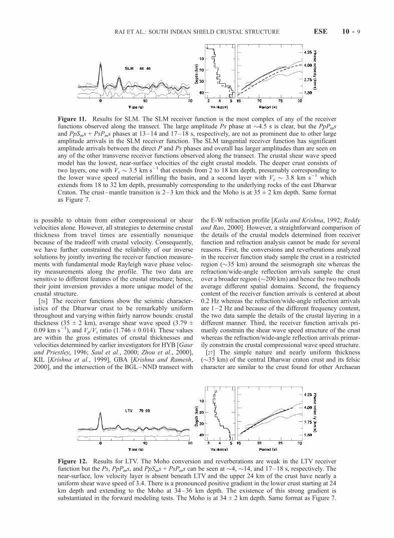
Figure 11. Results for SLM. The SLM receiver function is the most complex of any of the receiverfunctions observed along the transect. The large amplitude Ps phase at �4.5 s is clear, but the PpPmsand PpSms + PsPms phases at 13–14 and 17–18 s, respectively, are not as prominent due to other largeamplitude arrivals in the SLM receiver function. The SLM tangential receiver function has significantamplitude arrivals between the direct P and Ps phases and overall has larger amplitudes than are seen onany of the other transverse receiver functions observed along the transect. The crustal shear wave speedmodel has the lowest, near-surface velocities of the eight crustal models. The deeper crust consists oftwo layers, one with Vs � 3.5 km s�1 that extends from 2 to 18 km depth, presumably corresponding tothe lower wave speed material infilling the basin, and a second layer with Vs � 3.8 km s�1 whichextends from 18 to 32 km depth, presumably corresponding to the underlying rocks of the east DharwarCraton. The crust–mantle transition is 2–3 km thick and the Moho is at 35 ± 2 km depth. Same formatas Figure 7.

Figure 12. Results for LTV. The Moho conversion and reverberations are weak in the LTV receiverfunction but the Ps, PpPms, and PpSms + PsPms can be seen at �4, �14, and 17–18 s, respectively. Thenear-surface, low velocity layer is absent beneath LTV and the upper 24 km of the crust have nearly auniform shear wave speed of 3.4. There is a pronounced positive gradient in the lower crust starting at 24km depth and extending to the Moho at 34–36 km depth. The existence of this strong gradient issubstantiated in the forward modeling tests. The Moho is at 34 ± 2 km depth. Same format as Figure 7.


cratons that have remained largely stable since cratoniza-tion. The two largest Archaean terrains of western Australia(the Pilbara and the Yilgarn cratons) have a predominantlyfelsic [Chevrot and van der Hilst, 2000] crust which in theircentral undisturbed regions is 33–36 km thick [Clitheroe at

al., 2000] and underlain by a sharp Moho. The cores ofArchaean Kaapvaal and Zimbabwe cratons of southernAfrica also have crustal thicknesses clustering between 34and 37 km [Nguuri et al., 2001], and a sharp Moho thatproduces clear and large amplitude Ps signals. Sites over the

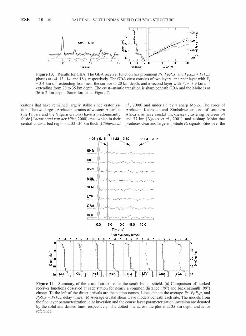
Figure 13. Results for GBA. The GBA receiver function has prominent Ps, PpPms, and PpSms + PsPmsphases at �4, 13–14, and 18 s, respectively. The GBA crust consists of two layers: an upper layer with Vs

�3.4 km s�1 extending from near the surface to 20 km depth, and a second layer with Vs � 3.9 km s�1

extending from 20 to 35 km depth. The crust–mantle transition is sharp beneath GBA and the Moho is at36 ± 2 km depth. Same format as Figure 7.

Figure 14. Summary of the crustal structure for the south Indian shield. (a) Comparison of stackedreceiver functions observed at each station for nearly a common distance (79�) and back azimuth (99�)cluster. To the left of the direct arrivals are the station names. Lines denote the average Ps, PpPms, andPpSms + PsPms delay times. (b) Average crustal shear wave models beneath each site. The models fromthe fine layer parameterization joint inversion and the coarse layer parameterization inversion are denotedby the solid and dashed lines, respectively. The dotted line across the plot is at 35 km depth and is forreference.


Slave craton in northwest Canada that contain the oldestknown rocks on Earth also show clear Ps phases withoutsignificant arrival time variations [Bank et al., 2000],yielding an average crustal thickness of 38 km. Receiverfunctions at three sites on the central Sao Francisco cratonin the southeast Brazilian shield show a similar �35 kmthick (estimated from the Ps � P intervals of 4–4.3 s),transparent crust which is felsic (Vp/Vs = 1.70) with nosignificant intracrustal features [Assumpcao et al., 2002].[28] Furthermore, there is no evidence for any high

velocity basal layer in the receiver function crustal imagesof the central Dharwar craton, suggesting that there is noseismically distinct layer of mafic cumulates overlying theMoho. This implies that the base of the Dharwar crust hasremained fairly refractory since its cratonization. Corrobo-rating evidence for the absence of mafic underplating in theDharwar craton is also provided by the average Poisson’sratio of the crust (0.256 ± 0.006), indicating that the crust isessentially intermediate-to-felsic in composition. This con-clusion supports the evolutionary hypothesis for the growthof continental crust; that is, the crustal formation processesin the Archean were different from those that dominatedsince the Archean [Durrheim and Mooney, 1991]. Indeed,the uniform low heat flow and the occurrence of diamondsin the Dharwar craton lend weight to this hypothesis.[29] Heat flow throughout this corridor is 25–50 mW

m�2 [Roy and Rao, 2000]. In fact, the mantle heat flow isreduced to a remarkably uniform value of around 12–18 mW m�2, when the quite variable heat generation ofthe surficial crustal layers is accounted for, discounting anysuggestion that there are substantial spatial variations in heatfrom the mantle into the lower crust. The eastern Dharwarcraton is also diamondiferous, with some of the well-knownpipes being quite close to LTV west of the CuddappahBasin. These diamonds, which are yet to be dated, occur inthe kimberlites of much younger ages (1100 Ma). SouthAfrican kimberlites of similar age contain Archean-agediamonds [Richardson et al., 1984].[30] The diamonds found on the Dharwar craton may also

belong to the Archean (2500 Ma) when the cratonization ofDharwar was complete, with an undercarriage of a colder,thicker lithosphere that had entered the diamond stabilityfield. A puzzling feature of the Dharwar craton, however, isthat its bulk composition does not appear to have akomatiitic origin but is possibly of tholeiitic and picriticcomposition, with some component of ultramafic rocks.[31] The above picture, strictly speaking, characterizes

only the central Dharwar craton whose 3-D structure mustawait similarly extended investigations to its east and west.The E-W refraction profile [Reddy and Rao, 2000], how-ever, indicates that the crust of the western Dharwar cratonacross the Closepet granite is thicker (>40 km) and of lowervelocity. However, based on its geology, the Dharwar cratonis widely regarded to be composed of two different terrainssutured longitudinally by the Closepet granite, and veryelaborate proposals [Hanson et al., 1986] have been sug-gested as evidence of a plate tectonic-type of activity havingoperated as far back as the Archean. Nevertheless, thesehypotheses are equivocal and if, as we believe, a similarevolutionary process was responsible for both the westernand eastern Dharwar craton, the differences in crustal thick-ness and isotopic signatures are a result of subsequent

tectonic processes. Therefore, we should be encouraged toinvestigate the western Dharwar craton for the possibleexistence of diamondiferous kimberlites and auriferousschists and not declare the western craton to be barren.[32] In conclusion, we note that seismically, the central

Dharwar craton over the 600 km long transect is remarkablytransparent and is therefore an excellent window for imag-ing the mantle beneath. The Dharwar craton appears to be aclassical representative of primitive cratons and constitutesa significant sample of early Earth processes that evolvedwith the thermodynamic evolution of the mantle.

[33] Acknowledgments. This project was supported in part by a grantfrom the Department of Science and Technology, Government of India, andby Bullard Laboratories of the University of Cambridge. Considerablelogistic support was provided by the directors of the National GeophysicalResearch Institute at Hyderabad, Centre for Mathematical Modeling andComputer Simulation, and the Indian Institute of Astrophysics at Banga-lore. VKG is especially thankful to Cowsik, Leelanandam, R. Srinivasan,and RUM Rao for stimulating discussions. KP would like to thank DenisHatzfeld for arranging a CNRS summer professorship and providingcomputing facilities at Universite Joseph Fourier, where most of thecomputations were done. This is Cambridge University Department ofEarth Sciences contribution 7145.

ReferencesAmmon, C. J., The isolation of receiver effects from teleseismic P wave-forms, Bull. Seismol. Soc. Am., 81, 2504–2510, 1991.

Ammon, C. J., G. E. Randall, and G. Zandt, On the non-uniqueness ofreceiver function inversions, J. Geophys. Res., 95, 15,303–15,318, 1990.

Assumpcao, M., D. James, and A. Snoke, Crustal thicknesses in SE Bra-zilian Shield by receiver function analysis: Implications for isostaticcompensation, J. Geophys. Res., 107(B1), 2006, doi:10.1029/2001JB000422, 2002.

Bank, C.-G., M. G. Bostock, R. M. Ellis, and J. F. Cassidy, A reconnais-sance teleseismic study of the upper mantle and transition zone beneaththe Archean Slave craton in NW Canada, Tectonophysics, 319, 151–166,2000.

Bhattacharya, S. N., Crustal and upper mantle velocity structure of Indiafrom surface wave dispersion, in Seismology in India: An Overview,edited by H. K. Gupta and S. Ramaseshan, Curr. Sci., 62, Suppl., 94–100, 1992.

Chatterjee, S. N., On the dispersion of Love Waves and crust –mantlestructure in the Gangetic Basin, Geophys. J. R. Astron. Soc., 23, 129–138, 1971.

Chevrot, S., and R. D. van der Hilst, The Poisson ratio of the Australiancrust: Geological and geophysical implications, Earth Planet. Sci. Lett.,183, 121–132, 2000.

Clitheroe, G., O. Gudmundsson, and B. L. N. Kennett, The crustal thick-ness of Australia, J. Geophys. Res., 105, 13,697–13,713, 2000.

Du, Z. J., and G. R. Foulger, The crustal structure of northwest Fjords,Iceland, from receiver functions and surface waves, Geophys. J. Int., 139,419–432, 1999.

Dube, R. K., J. C. Bhayana, and H. M. Chaudhary, Crustal structure of thePeninsular India, Pure Appl. Geophys., 109, 1718–1727, 1973.

Durrheim, R. J., and W. D. Mooney, Archean and Proterozoic crustal evo-lution: Evidence from crustal seismology, Geology, 19, 606–609, 1991.

Gaur, V. K., and K. Priestley, Shear wave velocity structure beneath theArchean granites around Hyderabad, inferred from receiver function ana-lysis, Proc. Indian Acad. Sci. Earth Planet. Sci., 105, 1–8, 1996.

Gaur, V. K., and K. F. Priestley, Shear wave velocity structure beneath theArchean granites around Hyderabad, inferred from receiver function ana-lysis, Proc. Indian Acad. Sci. Earth Planet. Sci., 106, 1–8, 1997.

Gomberg, J. S., K. Priestley, T. G. Masters, and J. N. Brune, The structureof the crust and upper mantle of northern Mexico, Geophys. J. R. Astron.Soc., 94, 1–20, 1988.

Hanson, G. N., E. J. Krogstad, V. Rajamani, and S. Balakrishnan, The Kolarschist belt: A possible Archean suture zone, in Workshop on TectonicEvolution of Greenstone Belts, edited by M. J. de Wit and L. D. Ashwal,LPI Tech Rep. 86-10, pp. 111–113, Lunar and Planet. Inst., Houston,Tex., 1986.

Herrmann, R. B., Computer Programs in Seismology, version 3.15, St.Louis Univ., St. Louis, Mo., 2002.

Huestis, S., P. Molnar, and J. Oliver, Regional Sn velocities and shearvelocity in the upper mantle, Bull. Seismol. Soc. Am., 63, 469–475, 1973.


Hwang, H. J., and B. J. Mitchell, Shear velocities, Qb, and frequencydependence of Qb in stable and tectonically active regions from surfacewave observations, Geophys. J. R. Astron. Soc., 90, 575–613, 1987.

Kaila, K. L. and V. G. Krishna, Deep seismic sounding studies in India andmajor discoveries, in Seismology in India: An Overview, edited by H. K.Gupta and S. Ramaseshan, Curr. Sci., 62, Suppl., 117–154, 1992.

Krishna, V. G., and D. S. Ramesh, Propagation of crustal waveguidetrapped Pg and seismic velocity structure in the south Indian shield, Bull.Seismol. Soc. Am., 90, 1281–1296, 2000.

Krishna, V. G., C. V. R. K. Rao, H. K. Gupta, D. Sarkar, and M. Baumbach,Crustal seismic velocity structure in the epicentral region of the Laturearthquake (September 29, 1993), southern India: Inferences from mod-elling of the aftershock seismograms, Tectonophysics, 304, 241–255,1999.

Kumar, M. R., J. Saul, D. Sarkar, R. Kind, and A. Shukla, Crustal structureof the Indian shield: New constraints from teleseismic receiver functions,Geophys. Res. Lett., 28, 1339–1342, 2001.

Nguuri, T. K., J. Gore, D. E. James, S. J. Webb, C. Wright, T. G. Zengeni,O. Gwavava, and J. A. Snoke, Crustal structure beneath southern Africaand its implications for the formation and evolution of the Kaapvaal andZimbabwe cratons, Geophys. Res. Lett., 28, 2501–2504, 2001.

Owens, T. J., G. Zandt, and S. R. Taylor, Seismic evidence for an ancientrift beneath the Cumberland Plateau, Tennessee: A detailed analysis ofbroadband teleseismic P waveforms, J. Geophys. Res., 89, 7783–7795,1984.

Priestley, K., G. Zandt, and G. Randal, Crustal structure in eastern Kazakh,USSR from teleseismic receiver functions, Geophys. Res. Lett., 15, 613–616, 1988.

Reddy, P. R., and V. Vijaya Rao, Structure and tectonics of the IndianPeninsular shield: Evidences from seismic velocities, Curr. Sci., 78,899–906, 2000.

Richardson, S. H., J. J. Gurney, A. J. Erlank, and J. W. Harris, Origin ofdiamonds in old enriched mantle, Nature, 310, 198–202, 1984.

Roy, S., and R. Rao, Heat flow in the Indian shield, J. Geophys. Res., 105,25,587–25,604, 2000.

Saul, J., M. R. Kumar, and D. Sarkar, Lithospheric and upper mantlestructure of the Indian shield, from teleseismic receiver functions, Geo-phys. Res. Lett., 27, 2357–2360, 2000.

Sheehan, A. F., G. A. Abers, C. H. Jones, and A. L. Lerner-Lam, Crustalthickness variation across the Colorado Rocky Mountains from teleseis-mic receiver functions, J. Geophys. Res., 100, 20,391–20,404, 1995.

Singh, S. K., R. S. Dattatrayam, N. M. Shapiro, P. Mandal, J. F. Pacheco,and R. K. Midha, Crustal and upper mantle structure of peninsular Indiaand source parameters of the 21 May 1997, Jabalpur earthquake (Mw =5,8): Results from the new regional broadband network, Bull. Seismol.Soc. Am., 89, 1631–1641, 1999.

Zandt, G., S. C. Myers, and T. C. Wallace, Crust and mantle structure acrossthe Basin and Range–Colorado Plateau boundary at 37�N latitude andimplementation for Cenozoic extensional mechanism, J. Geophys. Res.,100, 10,529–10,548, 1995.

Zhou, L., W.-P. Chen, and S. Ozalaybey, Seismic properties of the CentralIndian shield, Bull. Seismol. Soc. Am., 90, 1295–1304, 2000.

Zhu, L., and H. Kanamori, Moho depth variation in southern Californiafrom teleseismic receiver functions, J. Geophys. Res., 105, 2969–2980,2000.

��Z. Du, Institute of Theoretical Geophysics, University of Cambridge,

Cambridge, UK. ([email protected])V. K. Gaur, Centre for Mathematical Modeling and Computer Simulation,

NAL Belur Campus, Bangalore 560037, India. ([email protected])K. Priestley, Bullard Laboratories, University of Cambridge, Madingley

Rise, Madingley Road, Cambridge, CB3 0EZ, UK. ([email protected])S. S. Rai, D. Srinagesh, and K. Suryaprakasam, National Geophysical

Research Institute, Hyderabad 500007, India. ( [email protected])


Documents

Crustal shear velocity structure of the south Indian shield