C

I

gbbp�n�1d

©

GEOPHYSICS, VOL. 72, NO. 3 �MAY-JUNE 2007�; P. U31–U46, 10 FIGS., 2 TABLES.10.1190/1.2710205

onic velocity model

gor Ravve1 and Zvi Koren1

a�apcaiFsblm

�tvamctsrmevsr

moNclmtbmtj

eived O; zvi@

ABSTRACT

The effect of gradually increasing velocity with depth incompacted sedimentary layers is described by asymptotical-ly bounded velocity models. These models are defined bythree intuitive parameters: the velocity, its vertical gradient atan initial depth level, and a bounded velocity value. Recently,we have introduced the exponential asymptotically bounded�EAB� model, which belongs to this family of velocity mod-els. We introduce another monotonically increasing and as-ymptotically bounded model, which approaches the asymp-totic value in a slower and smoother fashion. Its main attrac-tiveness is the simplicity of ray tracing. The ray trajectories inthis model are elliptic, hyperbolic, or parabolic curves, de-pending on the ray parameter �horizontal slowness�. The lin-ear velocity model with a circular trajectory is a particularcase of the proposed model. Because the shapes of the ray tra-jectories correspond to the three types of conic sections, wecall the model Conic. We derive the relationships for lateralpropagation distance, traveltime, and arc length of the ray-path for arbitrary nonvertical rays, and we develop proce-dures for initial value and boundary-value ray tracing. Bothray-tracing problems have an analytical closed-formsolution.

INTRODUCTION

In compacted sedimentary layers, the instantaneous velocityradually increases with depth approaching a limiting value, definedy the properties of the fully compacted material. To describe thisehavior, different velocity models have been proposed. The sim-lest and the most widely used are the piecewise-constant modelDix, 1955; Hubral and Krey, 1980�, the linear velocity model �Slot-ick, 1936a, b, 1959�, the classical unbounded exponential modelSlotnick, 1936a, b�, and the linear slowness model �Al-Chalabi,997�. All these classical velocity models are unbounded at largeepths. They require a considerable number of depth intervals to

Manuscript received by the EditorAugust 16, 2006; revised manuscript rec1Paradigm Geophysical, Herzliya, Israel. E-mail: igorr@paradigmgeo.com2007 Society of Exploration Geophysicists.All rights reserved.

U31

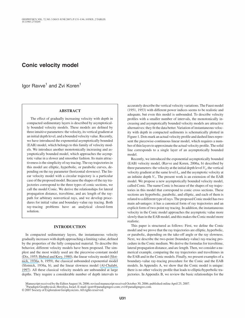
ccurately describe the vertical velocity variations. The Faust model1951, 1953� with different power indices seems to be realistic anddequate, but even this model is unbounded. To describe velocityrofiles with a smaller number of intervals, the monotonically in-reasing and asymptotically bounded velocity models are attractivelternatives: they fit the data better. Variation of instantaneous veloc-ty with depth in compacted sediments is schematically plotted inigure 1. Dots mark an actual velocity profile and dashed lines repre-ent the piecewise-continuous linear model, which requires a num-er of thin layers to approximate the actual velocity profile. The solidine corresponds to a single layer of an asymptotically bounded

odel.Recently, we introduced the exponential asymptotically bounded

EAB� velocity model, �Ravve and Koren, 2006a, b� described byhree parameters: the velocity at the initial depth level Va, the verticalelocity gradient at the same level ka, and the asymptotic velocity atn infinite depth V�. The present work is an extension of the EABodel. We propose a new asymptotically bounded velocity model,

alled Conic. The name Conic is because of the shapes of ray trajec-ories in this model that correspond to conic cross sections. Theseections are hyperbolic, parabolic, and elliptic, and each of them iselated to a different type of rays. The proposed Conic model has twoain advantages: it has a canonical form of ray trajectories and an

xplicit form of two-point ray tracing. In addition, the instantaneouselocity in the Conic model approaches the asymptotic value morelowly than in the EAB model, and this makes the Conic model moreealistic.

This paper is structured as follows: First, we define the Conicodel and we prove that the ray trajectories are elliptic, hyperbolic,

r parabolic, depending on the take-off angle or the ray slowness.ext, we describe the two-point �boundary-value� ray-tracing pro-

edure in the Conic medium. We derive the formulas for traveltime,ateral propagation distance, and arc length. Then, we consider a nu-

erical example, comparing the ray trajectories and traveltimes inhe EAB and in the Conic models. Finally, we present examples of aoundary-value ray-tracing procedure for the Conic and the EABodels. In Appendix A, we show that the Conic model is unique:

here is no other velocity profile that leads to elliptic/hyperbolic tra-ectories. In Appendix B, we review the basic relationships for the

ctober 30, 2006; published onlineApril 25, 2007.paradigmgeo.com.

taTbtpsdttCeVbt

ads

�

zt�edlwd

Akt0

cd

T

Fvm

ic

waumutm

Ds

Ir

wvr

Fvcpmeg

U32 Ravve and Koren

ilt �ray angle� and curvature of elliptic and hyperbolic trajectories,nd we relate the velocity and its gradient to the ray angle and depth.hese relations are further used to develop the initial value and theoundary-value ray-tracing procedures. In Appendix C, we derive aechnique for the initial value ray tracing. InAppendices D and E, weresent the two-point �boundary-value� ray-tracing technique, con-idering the endpoints located at different depths and at the sameepth, respectively. In Appendix F, we explain a technique of rayracing, through a reflector. In Appendix G, we study two-point rayracing through a package of horizontal layers described by differentonic velocity profiles with discontinuous velocity and/or its gradi-nt at the interfaces. In Appendix H, we consider the limit case

�→� when the Conic model converges to a linear velocity distri-ution, and we show that the traveltime derived for curved rays ofhe Conic model coincides with the traveltime for circular rays.

This paper refers to a class of laterally invariant 1D models, whichre naturally used in curved ray tomography in the time-migratedomain. General 3D complex models are beyond the scope of thistudy.

THE CONIC MODEL

We define the Conic velocity model as an infinite half-space 0�z�, where the velocity versus depth z is given by

V�z� =R�z + h�

�1 + Q2�z + h�2=

Rz

�1 + Q2z2, �1�

= z + h is the “absolute” depth, and R, Q, and h are three parame-ers that describe the model. Parameter h is a vertical shift: at z = −habove the reference depth level� the instantaneous velocity vanish-s. We call this point the absolute origin, z = 0. Parameter Q is aepth scale factor. It is also a measure of the nonlinearity of the ve-ocity function since Q→0 corresponds to the linear velocity modelith an unbounded velocity. The velocity gradient monotonicallyecreases with depth until it becomes infinitesimal:

0

1000

2000

3000

4000

5000

6000

7000

Dep

th (

m)

1000 2000 3000 4000 5000 6000Velocity (m/s)

Actual velocity profile

Asymptotically bounded model

Linear model

igure 1. Ageneral asymptotically bounded velocity model: verticalelocity variation. In this example, the actual velocity profile in theompacted sediments under the sea bottom �bold dots� can be ap-roximated either by a single layer of the asymptotically boundedodel with gradually decreasing gradient �solid line� or by three lin-

ar intervals with piecewise-constant and successively decreasingradients �dashed lines�.

k�z� =dV�z�

dz=

R

�1 + Q2�z + h�2�3/2 =R

�1 + Q2z2�3/2 . �2�

t the absolute origin, the velocity gradient has a maximum value,max = R. Within the depth range h� z�� �i.e., z�0�, the range ofhe velocity is Va �V�z��V�, and the range of the gradient is�k�z��ka.The Conic model can be also described in terms of the three physi-

al parameters mentioned previously: initial velocity Va, initial gra-ient ka, and asymptotic velocity V�,

Va =hR

�1 + Q2h2, ka =

R

�1 + Q2h2�3/2 , V� =R

Q. �3�

he inverse relationships are

R =kaV�

3

�V�2 − Va

2�3/2 , Q =R

V�

, h =Va�V�

2 − Va2�

kaV�2 . �4�

or a finite asymptotic velocity V� ��, we introduce the normalizedelocity V and the normalized absolute depth z. This leads to the nor-alized Conic velocity profile that includes no parameters,

V =V

V�

, z = Qz → V =z

�1 + z2. �5�

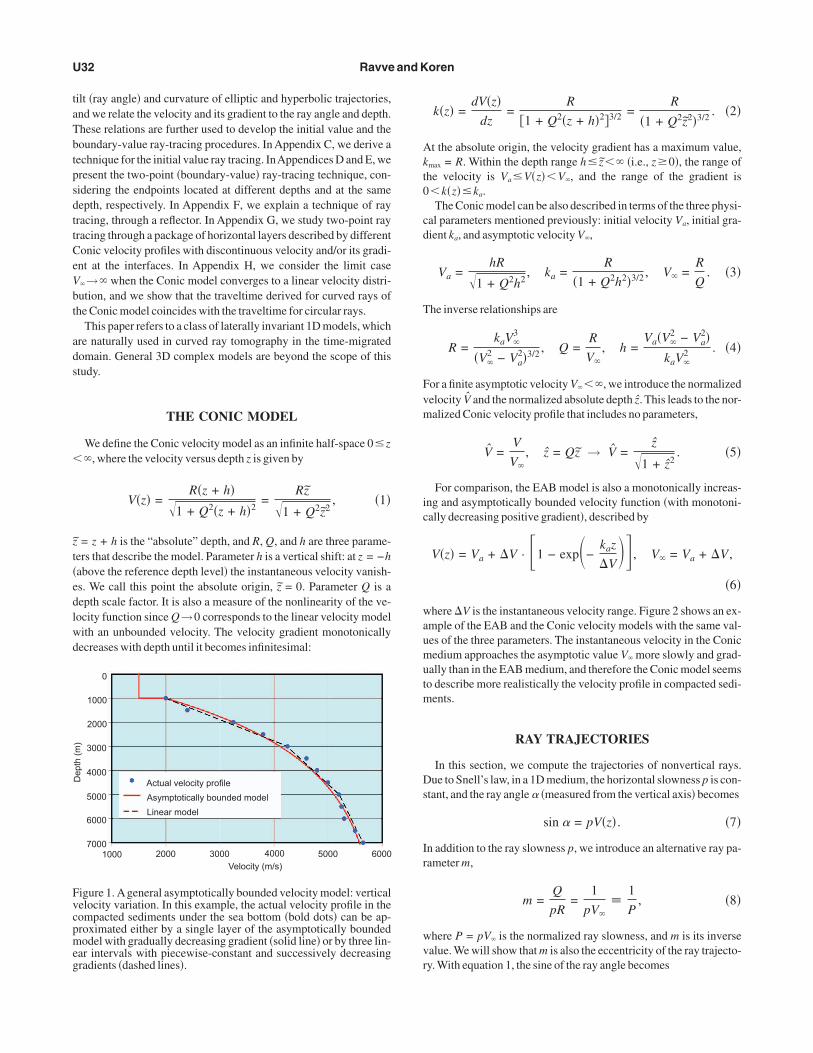
For comparison, the EAB model is also a monotonically increas-ng and asymptotically bounded velocity function �with monotoni-ally decreasing positive gradient�, described by

V�z� = Va + �V · �1 − exp�−kaz

�V�, V� = Va + �V ,

�6�

here �V is the instantaneous velocity range. Figure 2 shows an ex-mple of the EAB and the Conic velocity models with the same val-es of the three parameters. The instantaneous velocity in the Conicedium approaches the asymptotic value V� more slowly and grad-

ally than in the EAB medium, and therefore the Conic model seemso describe more realistically the velocity profile in compacted sedi-

ents.

RAY TRAJECTORIES

In this section, we compute the trajectories of nonvertical rays.ue to Snell’s law, in a 1D medium, the horizontal slowness p is con-

tant, and the ray angle � �measured from the vertical axis� becomes

sin � = pV�z� . �7�

n addition to the ray slowness p, we introduce an alternative ray pa-ameter m,

m =Q

pR=

1

pV�

1

P, �8�

here P = pV� is the normalized ray slowness, and m is its inversealue. We will show that m is also the eccentricity of the ray trajecto-y. With equation 1, the sine of the ray angle becomes

s

wm

w

E

w

Et

Tltnprcavt

ktrtirprdb

p

Ittwma

�cp

Rt=

wvv

tnqmutAv

Fdats

Conic velocity model U33

sin � =pRz

�1 + Q2z2=

pRz

�1 + m2p2R2z2, �9�

o that the tangent of this angle is

tan � = ±sin �

�1 − sin2 �= ±

pRz

�1 − m�2p2R2z2=

dx

dz, �10�

here m� is the conjugate eccentricity, m�2 = 1 − m2, and parameter�2 may be positive or negative. Integrating equation 10, we obtain

x�z� − xC = � tan �dz = ±�1 − m�2p2R2z2

m�2pR, �11�

here xC is the constant of integration. This leads to

p2R2m�4 · �x − xC�2 + p2R2m�2 · z2 = 1. �12�

quation 12 may be rearranged as

�x − xC�2

A2 ±z2

B2 = 1, �13�

here parameters A and B are

A2 =1

m�4p2R2 , ± B2 =1

m�2p2R2 . �14�

quation 13 describes a trajectory of elliptic or hyperbolic type, withhe eccentricity

e =�A2 � B2

A= m or e =

1

pV�

=1

P. �15�

he upper sign in equations 13–15 corresponds to an ellipse, and theower sign to a hyperbola. In both cases, the eccentricity is equal tohe inverse of the normalized slowness. Depending on the ray slow-ess p, parameters A and B are the semi-axes of an ellipse or of a hy-erbola. We distinguish three types of rays: precritical hyperbolicays when m�1, postcritical elliptic rays when 0�m�1, and criti-al parabolic rays when m = 1. For a linear velocity model, m = 0nd all rays are postcritical with a circular trajectory of constant cur-ature pR. Integrating equation 10 for the critical case m = 1, we ob-ain a parabola:

x − xC = ±Qz2

2. �16�

Thus, in the Conic velocity medium with the given parameters Va,a, and V�, we can have either of two kinds of rays, depending onheir horizontal slowness. The first kind — precritical hyperbolicays pV� �1 — may propagate to an infinite depth. At large depth,he instantaneous velocity becomes nearly constant, and the pre-crit-cal rays are nearly straight. The second kind — postcritical ellipticays, pV� �1 — first propagate downward, then reach a turningoint and return to the surface. In the limit case of critical parabolicays pV� = 1, the propagation depth is unbounded. At an infiniteepth, the parabolic rays become nearly horizontal; however, para-olic rays have no asymptote.

For any velocity model, the curvature of the ray trajectory isroportional to the vertical gradient of velocity,

�z� = pk�z� . �17�

n particular, in the linear velocity field with a constant gradient k,he curvature of a trajectory is constant for a fixed ray, and the trajec-ories are circular arcs. For the Conic model, the curvature decreasesith depth. Elliptic rays reach a minimum curvature at the lower-ost turning point. Hyperbolic rays become asymptotically straight

t an infinite depth.We now compute the critical angle �C. Rays with take-off angles

ray angle at the starting point on the earth’s surface� below the criti-al value �a ��C propagate to an infinite depth with a hyperbolicath. Their asymptotic tilt can be established from Snell’s law,

p =sin �a

Va=

sin ��

V�

→ �� = arcsinsin �aV�

Va

= arcsin�pV�� = arcsin1

m. �18�

ays with take-off angles exceeding the critical value �a ��C returno the surface following an elliptic path. For the critical angle, �a

�C, the normalized slowness is one, P = 1. This leads to

P = pCV� =sin �CV�

Va= 1 → �C = arcsin

Va

V�

, �19�

here pC is the critical slowness. Note that equations 18 and 19 arealid for any monotonically increasing and asymptotically boundedelocity model, not necessarily Conic or EAB.

The main advantage of the Conic model is the simplicity of thewo-point ray-tracing procedure. While the EAB model leads to aonlinear equation with an unknown ray parameter, which in turn re-uires an iterative procedure �Ravve and Koren, 2006a, b�, the Conicodel leads to an explicit solution. The Conic velocity model is

nique. There is no other 1D velocity distribution that leads to ellip-ic/hyperbolic rays. The proof of its uniqueness is given inAppendix. We start from the trajectory equation and we derive the velocityersus depth law.

12

1 - EAB model2 - Conic model

0

3000

6000

9000

12,000

15,0003000

Dep

th (

m)

4000 5000 6000Velocity (m/s)

igure 2. Instantaneous velocity of EAB and Conic model versusepth. The top velocity Va = 3000 m/s, the top gradient ka = 1 s−1,nd the asymptotic velocity V� = 6000 m/s. In the Conic model,he instantaneous velocity approaches the asymptotic value morelowly.

lci

Tt

I

C

Tcde

da1

wpe

wft

Em

Tgj

I

w

I

Tl

t

U34 Ravve and Koren

MAXIMUM PENETRATION DEPTH

The maximum penetration depth of over-critical elliptic rays isimited. The maximum velocity Vmax and the maximum depth zmax

orrespond to the turning point with the ray angle � = /2. Accord-ng to Snell’s law,

pVa = sin �a, pVmax = 1 → Vmax =1

p=

Va

sin �a. �20�

he maximum depth and the maximum velocity are related by equa-ion 1,

Vmax =R�zmax + h�

�1 + Q2�zmax + h�2→ �21�

zmax =Va

�R2 sin2 �a − Q2Va2

− h .

t follows from equations 3 and 19 that

R = QV�, R =ka

cos3 �C, h =

Va cos2 �C

ka. �22�

ombining equations 21 and 22, we obtain

zmax =Va cos2 �C

ka· � cos �C

�sin2 �a − sin2 �C

− 1� . �23�

he maximum absolute depth zmax = zmax + h gives the minor �verti-al� semi-axis B of the ellipse. Note that the maximum penetrationepth is different for various asymptotically bounded velocity mod-ls.

LATERAL DISTANCE, TRAVELTIME,AND ARC LENGTH

In a 1D medium, it is convenient to express the lateral propagationistance x, traveltime tS, and arc length s through the ray angle � andngle-dependent gradient k���. These relationships are �Kaufman,953; Ravve and Koren, 2006a, b�

x =1

p��a

�b

sin �d�

k���, tS = �

�a

�b

d�

sin �k���, s =

1

p��a

�b

d�

k���,

�24�

here �a and �b are ray angles at the departure and the destinationoints, respectively. It follows from Snell’s law �equation 7� andquations 1, 2, and 8 that

k��� = R · �1 − m2 sin2 ��3/2 R�3. �25�

here ��m,�� = �1 − m2 sin2 �. Equations 26–31 below followrom equations 24 and 25. The normalized lateral propagation dis-ance is

pRx = �− cos �

m�2��

�=�a

�=�b

. �26�

quation 26 can be used for m�1 and m�1. The parabolic case= 1 will be considered later. The normalized ray traveltime reads

RtS = −m2

m�2 ·cos �

�− arctanh� cos �

��

�=�a

�=�b

for m � 1, elliptic,

RtS = −m2

m�2 ·cos �

�− arctanh� �

cos ��

�=�a

�=�b

for m � 1, hyperbolic. �27�

he normalized arc length s = pRs is expressed through elliptic inte-rals of the first kind F and the second kind E. In case of elliptic tra-ectory, the eccentricity m�1 and

s =E��,m�

m�2 −m2

m�2 ·� sin � cos �

��

�=�a

�=�b

. �28�

n case of hyperbolic trajectory, the eccentricity m�1 and

s =E��,1/m�

m�2/m+

F��,1/m�m

−m2

m�2 · � sin � cos �

��

�=�a

�=�b

,

�29�

here the elliptic integrals are defined as

�30�

n case of a parabolic trajectory, m = 1, k��� = R cos3 � and

pRx =� 1

2 cos2 ��

� = �a

� = �b

,

RtS =� 1

2 cos2 �+ ln tan � �

� = �a

� = �b

,

pRs =1

2·�� sin �

cos2 �+ ln tan��

2+

4��

� = �a

� = �b

. �31�

he current depth can be also expressed through the ray angle. It fol-ows from equation 1,

z��� =V

R�1 − V2/V�2

→

Q · �zb − za� =�m sin �

��m,���

� = �a

� = �b

. �32�

INITIAL VALUE RAY TRACING

In the initial value ray-tracing problem, the medium parameters,he starting point, and the take-off ray angle are given, and the trajec-

tdcpartcf

CstlcttlsaerIflti

fuanldmFFltm�=ittnFdpe

Fmorva

Fzes

FEfigdprvature is larger.

Conic velocity model U35

ory is to be found.Applying equation 26 for angle-dependent lateralistance �x��� and equation 32 for angle-dependent depth z���, wean trace the ray trajectory parametrically, using the ray angle � as aarameter. An alternative, however, is to define explicitly the semi-xes A and B of the raypath and the lateral location xC of the trajecto-y center. The three conditions are: �1� the trajectory passes throughhe starting point �xa,za�, �2� the initial tilt is �a, and �3� the initialurvature is defined by the initial gradient a = pka. The techniqueor the initial value ray tracing is presented inAppendix C.

BOUNDARY VALUE RAY TRACING

The two-point ray-tracing problem has a simple solution for theonic velocity model. The given data are the depth values of the

ource and the destination points za and zb and the lateral distance be-ween these two points. The three parameters to be found are the el-iptic or hyperbolic semi-axes and the lateral location of the raypathenter. We distinguish two cases: a case when the source and the des-ination points are located at different depths, and a case when thewo endpoints are located at the same depth level �full symmetric el-iptic arc�. We treat these two cases differently. In both cases, the re-olving set of three equations has an analytic closed-form solution,nd this makes the Conic model especially attractive among the oth-r asymptotically bounded models. The technique of the two-pointay tracing is derived in Appendices D �case one� and E �case two�.n addition, we consider the ray-tracing procedure through the re-ector, and this technique is explained in Appendix F. Finally, ray

racing through a package of layers with the Conic velocity profiless studied inAppendix G.

NUMERICAL COMPARISON OF THE EABAND THE CONIC MODEL

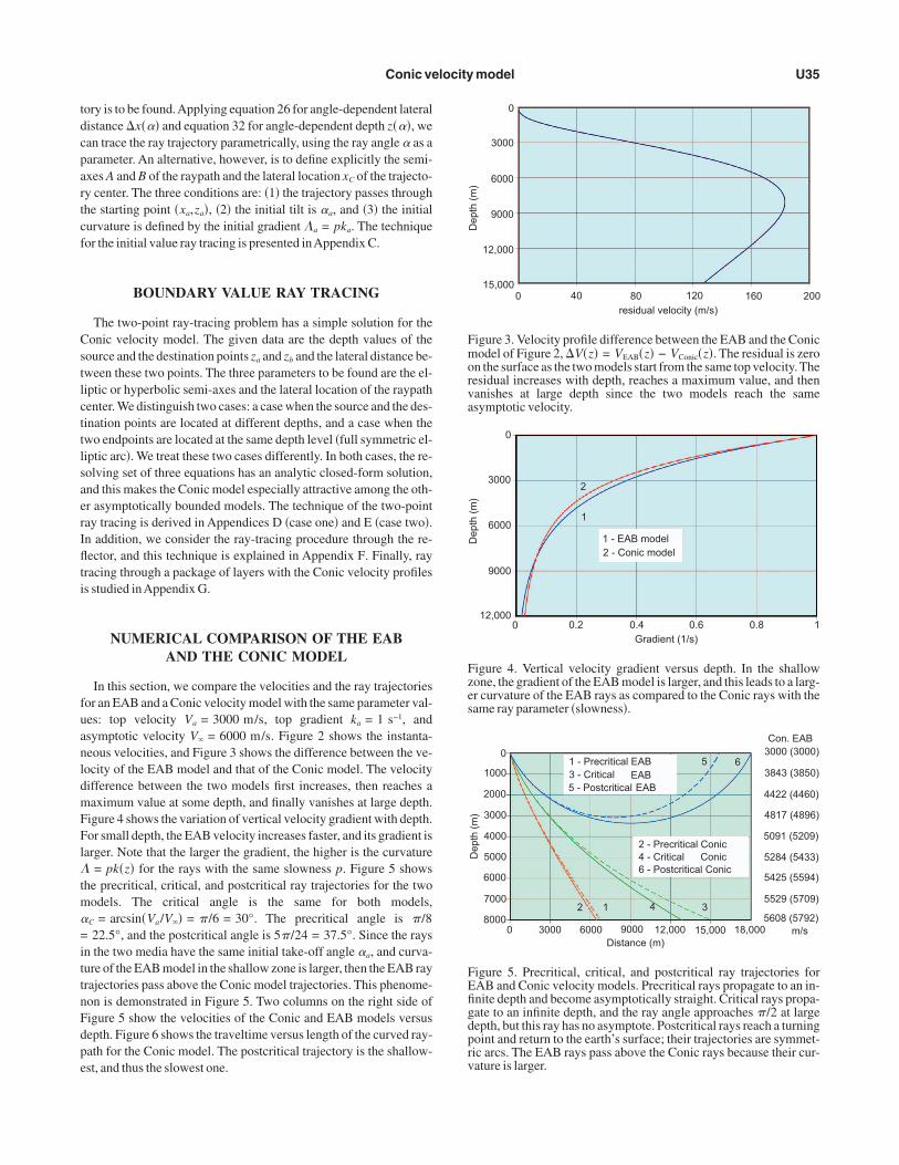
In this section, we compare the velocities and the ray trajectoriesor an EAB and a Conic velocity model with the same parameter val-es: top velocity Va = 3000 m/s, top gradient ka = 1 s−1, andsymptotic velocity V� = 6000 m/s. Figure 2 shows the instanta-eous velocities, and Figure 3 shows the difference between the ve-ocity of the EAB model and that of the Conic model. The velocityifference between the two models first increases, then reaches aaximum value at some depth, and finally vanishes at large depth.igure 4 shows the variation of vertical velocity gradient with depth.or small depth, the EAB velocity increases faster, and its gradient is

arger. Note that the larger the gradient, the higher is the curvature= pk�z� for the rays with the same slowness p. Figure 5 shows

he precritical, critical, and postcritical ray trajectories for the twoodels. The critical angle is the same for both models,

C = arcsin�Va/V�� = /6 = 30°. The precritical angle is /822.5°, and the postcritical angle is 5/24 = 37.5°. Since the rays

n the two media have the same initial take-off angle �a, and curva-ure of the EAB model in the shallow zone is larger, then the EAB rayrajectories pass above the Conic model trajectories. This phenome-on is demonstrated in Figure 5. Two columns on the right side ofigure 5 show the velocities of the Conic and EAB models versusepth. Figure 6 shows the traveltime versus length of the curved ray-ath for the Conic model. The postcritical trajectory is the shallow-st, and thus the slowest one.

0

3000

6000

9000

12,000

15,000

Dep

th (

m)

0 40 80 120 160 200residual velocity (m/s)

igure 3. Velocity profile difference between the EAB and the Conicodel of Figure 2, �V�z� = VEAB�z� − VConic�z�. The residual is zero

n the surface as the two models start from the same top velocity. Theesidual increases with depth, reaches a maximum value, and thenanishes at large depth since the two models reach the samesymptotic velocity.

2

1

0

3000

6000

9000

12,000

Dep

th (

m)

0

1 - EAB model2 - Conic model

0.2 0.4 0.6 0.8 1Gradient (1/s)

igure 4. Vertical velocity gradient versus depth. In the shallowone, the gradient of the EAB model is larger, and this leads to a larg-r curvature of the EAB rays as compared to the Conic rays with theame ray parameter �slowness�.

1 - Precritical EAB3 - Critical EAB5 - Postcritical EAB

2 - Precritical Conic4 - Critical Conic6 - Postcritical Conic

5 6

2 1 4 3

0

1000

2000

3000

4000

5000

6000

7000

8000

Dep

th (

m)

3000 (3000)Con. EAB

3843 (3850)

4422 (4460)

4817 (4896)

5091 (5209)

5284 (5433)

5425 (5594)

5529 (5709)

5608 (5792)m/s0 3000 6000 9000 12,000 15,000 18,000

Distance (m)

igure 5. Precritical, critical, and postcritical ray trajectories forAB and Conic velocity models. Precritical rays propagate to an in-nite depth and become asymptotically straight. Critical rays propa-ate to an infinite depth, and the ray angle approaches /2 at largeepth, but this ray has no asymptote. Postcritical rays reach a turningoint and return to the earth’s surface; their trajectories are symmet-ic arcs. The EAB rays pass above the Conic rays because their cur-

ppblplftmpeB=wl�e

ctpccc

stlmtxtppzoKtTgirprAmbCrj

ctdecaBm

Fam

Ftaftljc

Fapat

U36 Ravve and Koren

EXAMPLES OF RAY TRACING IN THE EABAND THE CONIC MODEL

In this section, we first consider three boundary-value ray-tracingroblems in a continuous Conic half-space, then we solve an exam-le of ray tracing through a reflector, and finally we demonstrate theoundary-value ray tracing through a package of layers. In two prob-ems with the continuous half-space, the source and the destinationoints are located at different depths. In the third problem, they areocated at the same depth and the approach for the ray tracing is dif-erent. We study the same medium: the top velocity Va = 3000 m/s,he top gradient ka = 1 s−1, and the asymptotic velocity V� = 6000

/s. We refer to Figure 7, which shows the solution of the first tworoblems. In both cases, the source point A is the same and it is locat-d at the origin. In the first case, the destination point is1�x = 4 km,z = 2 km�, and in the second case B2�x = 2 km,z3 km�. The goal is to plot the ray trajectory. First, we determinehether the trajectories are hyperbolic or elliptic. For this we calcu-

ate the critical angle �C = 30° and plot the critical parabolic raygreen line in Figure 7�. We see that the destination point B1 is locat-d above the critical ray, while the destination point B2 is below the

5

4

3

2

1

00 5000 10,000 15,000 20,000

Ray arc length (m)

Tim

e (s

)

1 - Precritical ray2 - Critical ray3 - Postcritical ray

3

2

1

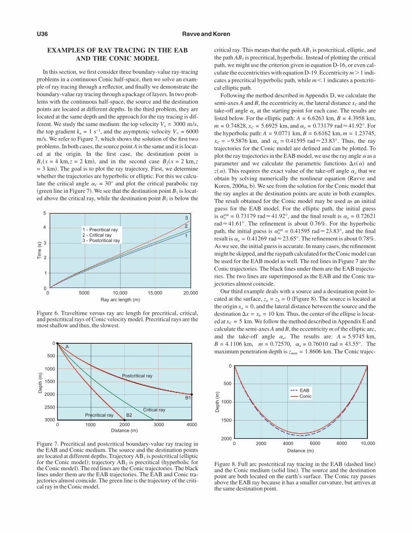
igure 6. Traveltime versus ray arc length for precritical, critical,nd postcritical rays of Conic velocity model. Precritical rays are theost shallow and thus, the slowest.

Postcritical ray

B1

A

Precritical ray B2Critical ray

0

500

1000

1500

2000

2500

3000

Dep

th (

m)

0 1000 2000 3000 4000Distance (m)

igure 7. Precritical and postcritical boundary-value ray tracing inhe EAB and Conic medium. The source and the destination pointsre located at different depths. Trajectory AB1 is postcritical �ellipticor the Conic model�; trajectory AB2 is precritical �hyperbolic forhe Conic model�. The red lines are the Conic trajectories. The blackines under them are the EAB trajectories. The EAB and Conic tra-ectories almost coincide. The green line is the trajectory of the criti-al ray in the Conic model.

ritical ray. This means that the path AB1 is postcritical, elliptic, andhe path AB2 is precritical, hyperbolic. Instead of plotting the criticalath, we might use the criterion given in equation D-16, or even cal-ulate the eccentricities with equation D-19. Eccentricity m�1 indi-ates a precritical hyperbolic path, while m�1 indicates a postcriti-al elliptic path.

Following the method described in Appendix D, we calculate theemi-axes A and B, the eccentricity m, the lateral distance xC and theake-off angle �a at the starting point for each case. The results areisted below. For the elliptic path: A = 6.6263 km, B = 4.3958 km,

= 0.74828, xC = 5.6925 km, and �a = 0.73179 rad 41.92°. Forhe hyperbolic path: A = 9.0771 km, B = 6.6162 km, m = 1.23745,

C = −9.5876 km, and �a = 0.41595 rad 23.83°. Thus, the rayrajectories for the Conic model are defined and can be plotted. Tolot the ray trajectories in the EAB model, we use the ray angle � as aarameter and we calculate the parametric functions �x��� and���. This requires the exact value of the take-off angle �a that webtain by solving numerically the nonlinear equation �Ravve andoren, 2006a, b�. We see from the solution for the Conic model that

he ray angles at the destination points are acute in both examples.he result obtained for the Conic model may be used as an initialuess for the EAB model. For the elliptic path, the initial guesss �a

init = 0.73179 rad 41.92°, and the final result is �a = 0.72621ad 41.61°. The refinement is about 0.76%. For the hyperbolicath, the initial guess is �a

init = 0.41595 rad 23.83°, and the finalesult is �a = 0.41269 rad 23.65°. The refinement is about 0.78%.s we see, the initial guess is accurate. In many cases, the refinementight be skipped, and the raypath calculated for the Conic model can

e used for the EAB model as well. The red lines in Figure 7 are theonic trajectories. The black lines under them are the EAB trajecto-

ies. The two lines are superimposed as the EAB and the Conic tra-ectories almost coincide.

Our third example deals with a source and a destination point lo-ated at the surface, za = zb = 0 �Figure 8�. The source is located athe origin xa = 0, and the lateral distance between the source and theestination �x = xb = 10 km. Thus, the center of the ellipse is locat-d at xC = 5 km. We follow the method described inAppendix E andalculate the semi-axes A and B, the eccentricity m of the elliptic arc,nd the take-off angle �a. The results are: A = 5.9745 km,= 4.1106 km, m = 0.72570, �a = 0.76010 rad = 43.55°. Theaximum penetration depth is zmax = 1.8606 km. The Conic trajec-

EABConic

0

500

1000

1500

2000

Dep

th (

m)

0 2000 4000 6000 8000 10,000

Distance (m)

igure 8. Full arc postcritical ray tracing in the EAB �dashed line�nd the Conic medium �solid line�. The source and the destinationoint are both located on the earth’s surface. The Conic ray passesbove the EAB ray because it has a smaller curvature, but arrives athe same destination point.

ttebttaiittssEas

teorlsstsdnitebd

S

1

2

3

4

5

6

tt

lcaT�ewtoed

tp=ctil�tvata=tppsT

TLv

L

1

2

3

FTc

Conic velocity model U37

ory is the solid line in Figure 8. To plot the EAB trajectory, we needo refine the take-off angle. For this, we solve again the nonlinearquation. Now the ray angle at the destination point is obtuse, andecause of the symmetry, the take-off angle �a is complementary tohe destination angle �b, so that �b = − �a. The result obtained forhe Conic model can be used as an initial guess for the EAB model,nd the refined result is �a = 0.74649 rad = 42.77°. The refinements about 1.79%. The maximum depth calculated for the EAB models zmax = 1.9195 km. The maximum depth relative difference be-ween the two models is about 3.17%. Unlike Figure 5, in Figure 8he Conic trajectory is above the EAB trajectory. The EAB pathtarts from a smaller take-off angle and penetrates deeper, so that de-pite the larger velocity gradient and the greater ray curvature in theAB model, the Conic ray and the EAB ray reach the earth’s surfacet the same point. In Figure 5, both the EAB and the Conic raypathstart from the same take-off angle.

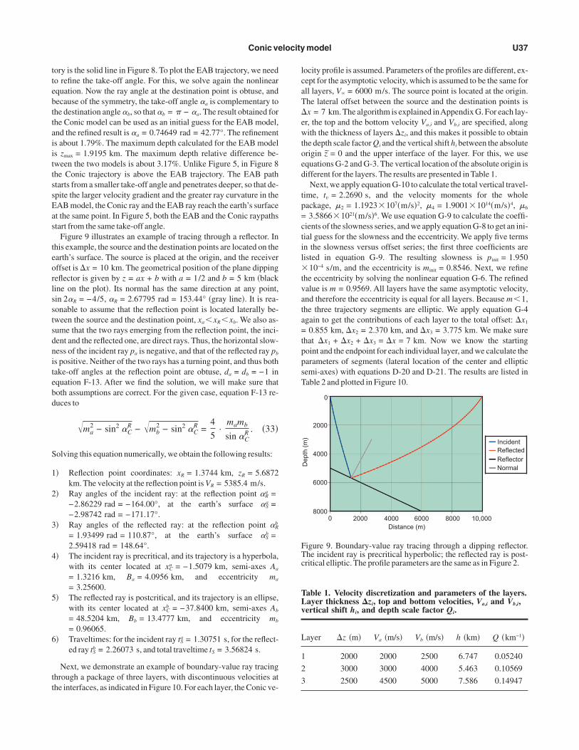
Figure 9 illustrates an example of tracing through a reflector. Inhis example, the source and the destination points are located on thearth’s surface. The source is placed at the origin, and the receiverffset is �x = 10 km. The geometrical position of the plane dippingeflector is given by z = ax + b with a = 1/2 and b = 5 km �blackine on the plot�. Its normal has the same direction at any point,in 2�R = −4/5, �R = 2.67795 rad = 153.44° �gray line�. It is rea-onable to assume that the reflection point is located laterally be-ween the source and the destination point, xa �xR �xb. We also as-ume that the two rays emerging from the reflection point, the inci-ent and the reflected one, are direct rays. Thus, the horizontal slow-ess of the incident ray pa is negative, and that of the reflected ray pb

s positive. Neither of the two rays has a turning point, and thus bothake-off angles at the reflection point are obtuse, da = db = −1 inquation F-13. After we find the solution, we will make sure thatoth assumptions are correct. For the given case, equation F-13 re-uces to

�ma2 − sin2 �C

R − �mb2 − sin2 �C

R =4

5·

mamb

sin �CR . �33�

olving this equation numerically, we obtain the following results:

� Reflection point coordinates: xR = 1.3744 km, zR = 5.6872km. The velocity at the reflection point is VR = 5385.4 m/s.

� Ray angles of the incident ray: at the reflection point �Ra =

−2.86229 rad = −164.00°, at the earth’s surface �Sa =

−2.98742 rad = −171.17°.� Ray angles of the reflected ray: at the reflection point �R

b

= 1.93499 rad = 110.87°, at the earth’s surface �Sb =

2.59418 rad = 148.64°.� The incident ray is precritical, and its trajectory is a hyperbola,

with its center located at xCa = −1.5079 km, semi-axes Aa

= 1.3216 km, Ba = 4.0956 km, and eccentricity ma

= 3.25600.� The reflected ray is postcritical, and its trajectory is an ellipse,

with its center located at xCb = −37.8400 km, semi-axes Ab

= 48.5204 km, Bb = 13.4777 km, and eccentricity mb

= 0.96065.� Traveltimes: for the incident ray tS

a = 1.30751 s, for the reflect-ed ray tS

b = 2.26073 s, and total traveltime tS = 3.56824 s.

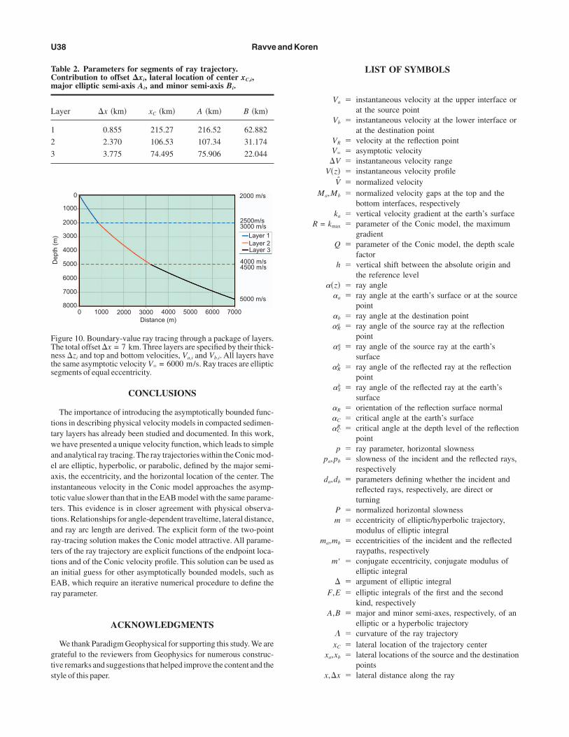
Next, we demonstrate an example of boundary-value ray tracinghrough a package of three layers, with discontinuous velocities athe interfaces, as indicated in Figure 10. For each layer, the Conic ve-

ocity profile is assumed. Parameters of the profiles are different, ex-ept for the asymptotic velocity, which is assumed to be the same forll layers, V� = 6000 m/s. The source point is located at the origin.he lateral offset between the source and the destination points isx = 7 km. The algorithm is explained inAppendix G. For each lay-r, the top and the bottom velocity Va,i and Vb,i are specified, alongith the thickness of layers �zi, and this makes it possible to obtain

he depth scale factor Qi and the vertical shift hi between the absoluterigin z = 0 and the upper interface of the layer. For this, we usequations G-2 and G-3. The vertical location of the absolute origin isifferent for the layers. The results are presented in Table 1.

Next, we apply equation G-10 to calculate the total vertical travel-ime, tv = 2.2690 s, and the velocity moments for the wholeackage, �2 = 1.1923�107�m/s�2, �4 = 1.9001�1014�m/s�4, �6

3.5866�1021�m/s�6. We use equation G-9 to calculate the coeffi-ients of the slowness series, and we apply equation G-8 to get an ini-ial guess for the slowness and the eccentricity. We apply five termsn the slowness versus offset series; the first three coefficients areisted in equation G-9. The resulting slowness is pinit = 1.950

10−4 s/m, and the eccentricity is minit = 0.8546. Next, we refinehe eccentricity by solving the nonlinear equation G-6. The refinedalue is m = 0.9569. All layers have the same asymptotic velocity,nd therefore the eccentricity is equal for all layers. Because m�1,he three trajectory segments are elliptic. We apply equation G-4gain to get the contributions of each layer to the total offset: �x1

0.855 km, �x2 = 2.370 km, and �x3 = 3.775 km. We make surehat �x1 + �x2 + �x3 = �x = 7 km. Now we know the startingoint and the endpoint for each individual layer, and we calculate thearameters of segments �lateral location of the center and ellipticemi-axes� with equations D-20 and D-21. The results are listed inable 2 and plotted in Figure 10.

able 1. Velocity discretization and parameters of the layers.ayer thickness �zi, top and bottom velocities, Va,i and Vb,i,ertical shift hi, and depth scale factor Qi.

ayer �z �m� Va �m/s� Vb �m/s� h �km� Q �km−1�

2000 2000 2500 6.747 0.05240

3000 3000 4000 5.463 0.10569

2500 4500 5000 7.586 0.14947

Incident Reflected Reflector Normal

0

2000

4000

6000

8000

Dep

th (

m)

0 2000 4000 6000 8000 10,000 Distance (m)

igure 9. Boundary-value ray tracing through a dipping reflector.he incident ray is precritical hyperbolic; the reflected ray is post-ritical elliptic. The profile parameters are the same as in Figure 2.

ttwaeaitttarttaEr

gts

TCm

L

1

2

3

FTnts

U38 Ravve and Koren

CONCLUSIONS

The importance of introducing the asymptotically bounded func-ions in describing physical velocity models in compacted sedimen-ary layers has already been studied and documented. In this work,e have presented a unique velocity function, which leads to simple

nd analytical ray tracing. The ray trajectories within the Conic mod-l are elliptic, hyperbolic, or parabolic, defined by the major semi-xis, the eccentricity, and the horizontal location of the center. Thenstantaneous velocity in the Conic model approaches the asymp-otic value slower than that in the EAB model with the same parame-ers. This evidence is in closer agreement with physical observa-ions. Relationships for angle-dependent traveltime, lateral distance,nd ray arc length are derived. The explicit form of the two-pointay-tracing solution makes the Conic model attractive. All parame-ers of the ray trajectory are explicit functions of the endpoint loca-ions and of the Conic velocity profile. This solution can be used asn initial guess for other asymptotically bounded models, such asAB, which require an iterative numerical procedure to define the

ay parameter.

ACKNOWLEDGMENTS

We thank Paradigm Geophysical for supporting this study. We arerateful to the reviewers from Geophysics for numerous construc-ive remarks and suggestions that helped improve the content and thetyle of this paper.

able 2. Parameters for segments of ray trajectory.ontribution to offset �xi, lateral location of center xC,i,ajor elliptic semi-axis Ai, and minor semi-axis Bi.

ayer �x �km� xC �km� A �km� B �km�

0.855 215.27 216.52 62.882

2.370 106.53 107.34 31.174

3.775 74.495 75.906 22.044

Layer 1Layer 2Layer 3

2000 m/s

2500m/s3000 m/s

4000 m/s4500 m/s

5000 m/s

0

1000

2000

3000

4000

5000

6000

7000

8000

Dep

th (

m)

0 1000 2000 3000 4000 5000 6000 7000Distance (m)

igure 10. Boundary-value ray tracing through a package of layers.he total offset �x = 7 km. Three layers are specified by their thick-ess �zi and top and bottom velocities, Va,i and Vb,i. All layers havehe same asymptotic velocity V� = 6000 m/s. Ray traces are ellipticegments of equal eccentricity.

LIST OF SYMBOLS

Va instantaneous velocity at the upper interface orat the source point

Vb instantaneous velocity at the lower interface orat the destination point

VR velocity at the reflection pointV� asymptotic velocity

�V instantaneous velocity rangeV�z� instantaneous velocity profile

V normalized velocityMa,Mb normalized velocity gaps at the top and the

bottom interfaces, respectivelyka vertical velocity gradient at the earth’s surface

R = kmax parameter of the Conic model, the maximumgradient

Q parameter of the Conic model, the depth scalefactor

h vertical shift between the absolute origin andthe reference level

��z� ray angle�a ray angle at the earth’s surface or at the source

point�b ray angle at the destination point�R

a ray angle of the source ray at the reflectionpoint

�Sa ray angle of the source ray at the earth’s

surface�R

b ray angle of the reflected ray at the reflectionpoint

�Sb ray angle of the reflected ray at the earth’s

surface�R orientation of the reflection surface normal�C critical angle at the earth’s surface�C

R critical angle at the depth level of the reflectionpoint

p ray parameter, horizontal slownesspa,pb slowness of the incident and the reflected rays,

respectivelyda,db parameters defining whether the incident and

reflected rays, respectively, are direct orturning

P normalized horizontal slownessm eccentricity of elliptic/hyperbolic trajectory,

modulus of elliptic integralma,mb eccentricities of the incident and the reflected

raypaths, respectivelym� conjugate eccentricity, conjugate modulus of

elliptic integral� argument of elliptic integral

F,E elliptic integrals of the first and the secondkind, respectively

A,B major and minor semi-axes, respectively, of anelliptic or a hyperbolic trajectory

curvature of the ray trajectoryxC lateral location of the trajectory center

xa,xb lateral locations of the source and the destinationpoints

x,�x lateral distance along the ray

mte

T

Wn

Av=

E

I

se

wss

I

FC

atittacu

we

T

NattC

Conic velocity model U39

�xa signed lateral distance between the source andthe reflection point

�xb signed lateral distance between the destinationand the reflection point

tS traveltime along the raytSa,tS

b traveltime along the incident and the reflectedrays, respectively

s ray arc lengths normalized ray arc lengthz depth measured from the earth’s surface or

upper interfacez, z absolute depth and normalized absolute depth,

respectivelyza,zb vertical locations of the source and the

destination pointxR,zR location of the reflection surface element

r parameter along the reflector linerR parameter on the reflector line, corresponding

to the reflection pointlX,lZ leading cosines of the tangent to the reflector

linenX

R,nZR leading cosines of the normal to the reflector

line� tilt of the secant line between the source and

the destination point

APPENDIX A

UNIQUENESS OF THE CONIC MODEL

In this appendix, we demonstrate the uniqueness of the Conicodel. Given the elliptic/hyperbolic trajectory of the raypath �equa-

ion 13�, we prove that the instantaneous velocity versus depth is giv-n by equation 1. Rearranging equation 13, we obtain

x − xC = ± A�1 � z2/B2. �A-1�

he tangent of the ray angle is

tan � =dx

dz= ±

Az

B2�1 � z2/B2. �A-2�

ithout any loss of generality, we may consider the horizontal slow-ess p positive. Thus, the sine of the ray angle is also positive,

sin � =1

�1 + cot2 �=

Az

�B4 + �A2 � B2� · z2. �A-3�

ccording to Snell’s law, in a 1D velocity model �with no lateralariation of velocity� the horizontal slowness is constant and sin �p ·V�z�. Thus, equation A-3 leads to

V�z� =1

p·

Az

�B4 + �A2 � B2� · z2. �A-4�

quation A-4 can be rearranged as

V−2�z� = p2 · �B4

A2 · z −2 +A2 � B2

A2 � . �A-5�

n an isotropic medium, velocity is independent of the specific ray

lowness p. Since this is true for any depth z, the two coefficients inquation A-5 are constant,

p2 ·B4

A2 = N1, p2 ·A2 � B2

A2 = N2, �A-6�

here N1 and N2 are constant values independent of p, while theemi-axes A and B depend on p. Solving equation set A-6 we find theemi-axes,

A2 =p2N1

�p2 − N2�2 , B2 = ±N1

p2 − N2→

A2 � B2 =N1 · N2

�p2 − N22�2 . �A-7�

ntroducing result A-7 into the velocity distribution A-4, we obtain

V�z� =z

�N1 + N2 · z2. �A-8�

inally, we set N1 = 1/R2 and N2 = Q2/R2 = V�−2, and we obtain the

onic velocity function, equation 1.

APPENDIX B

TILT AND CURVATURE OF ELLIPTICAND HYPERBOLIC TRAJECTORIES

In this appendix, we review the basic relationships for the tilt �rayngle� of elliptic and hyperbolic trajectories, to be further used in ini-ial value and boundary-value ray tracing. For two-point ray tracing,t is suitable to work in the shifted frame of reference. As we men-ioned, in the shifted frame depth z is measured from the origin abovehe earth’s surface.At z = 0, the instantaneous velocity vanishes andll rays �actually, continuations of rays� become vertical, so that theenters of ellipses or hyperbolas are located there. In the Conic medi-m, the shapes of rays are second-order curves,

�B-1�

here xC is the horizontal distance of the raypath.At any point of thelliptic or hyperbolic trajectory, the ray angle is

sin � =A2z

�A4z2 + B4�x − xC�2. �B-2�

he curvature of both elliptic or hyperbolic line z�x� is

=z�

�1 + z�2�3/2 = −A4B4

�A4z2 + B4�x − xC�2�3/2 . �B-3�

ormally, the curvature of an ellipse or hyperbola is considered neg-tive, but we will need to change the sign on the right side of equa-ion B-1 because ray angles are measured from the vertical axis, andhus, for a positive horizontal slowness, the ray angles increase.ombine equations B-2 and B-3,

Bp

wa

Nj

�tpt�cBil

Td

W

T

Wt

R

C

wfc

wpE

Ndac

wF

Nt

ep

erltp

U40 Ravve and Koren

��� =B4 sin3 �

A2z3 . �B-4�

ecause of Snell’s law, in any 1D medium, the curvature of the ray-ath is

��� =k��� · sin �

V���, �B-5�

here k��� is the angle-dependent velocity gradient. Equations B-4nd B-5 result in

B4 sin2 �

A2z3 =k���V���

. �B-6�

ote that although equation B-6 is related to the curvature of the tra-ectory, the curvature is eliminated from this equation.

APPENDIX C

TECHNIQUE FOR INITIAL VALUE RAY TRACING

Given the three parameters of the Conic model, the starting pointxa,za�, and the initial ray angle �a, we find the semi-axes A and B ofhe trajectory and the lateral distance xC of its center. First, we com-are the ray angle with the critical angle �C = arcsin�Va/V�� in ordero define whether the raypath is elliptic �postcritical� or hyperbolicprecritical�. To find the semi-axes and the distance, we apply threeonditions: the trajectory passes through the starting point �equation-1�, the initial tilt is known �equation B-2�, and the initial curvature

s known �equation B-6�. The introduction of equation B-6 into B-2eads to

zaka�xa − xC�2 = A2Va cos2 �a. �C-1�

his equation may be further simplified. Solving equation 1 forepth z,

R2z2�1 − Va2/V�

2 � = Va2 → Va = Rz cos �C. �C-2�

ith the use of the second equation of set 22, equation C-2 becomes

Va =kaza

cos2 �C→ za =

Va cos2 �C

ka. �C-3�

his makes it possible to eliminate depth from equation C-1,

�xa − xC�2

A2 =cos2 �a

cos2 �C. �C-4�

ith the use of equations C-3 and C-4, the equation of the ray trajec-ory B-1 reduces to

±Va

2

ka2 ·

cos4 �C

B2 =cos2 �C − cos2 �a

cos2 �C=

sin2 �a − sin2 �C

cos2 �C

=sin2 �a

cos2 �C· �1 −

sin2 �C

sin2 �a� . �C-5�

ecall that the eccentricity can be presented as

sin �C

sin �a=

Va/V�

pVa=

1

pV�

= m . �C-6�

ombining equations C-5 and C-6,

±Va

2

ka2 ·

cos4 �C

B2 =sin2 �a

cos2 �C· �1 − m2� =

sin2 �am�2

cos2 �C,

�C-7�

here the conjugate eccentricity squared m�2 = 1 − m2 is positiveor an ellipse and negative for a hyperbola. The minor semi-axis be-omes

B =Va

ka·

cos3 �C

sin �a·

1�± m�2

, �C-8�

here the plus sign stands for an ellipse and the minus sign for a hy-erbola, so that the value under the square root is positive anyway.quations B-6, C-3, and C-8 yield the major semi-axis,

A =ka

Va·

B2 sin �a

cos3 �C=

Va

ka·

cos3 �C

sin �a·

1

± m�2 =B

�± m�2.

�C-9�

ext, we use C-4 to get the distance xC. Analyzing the signs of theistances in case of an ellipse or a hyperbola, for acute and obtuse rayngles �obtuse angles may occur only in case of an ellipse�, we con-lude that for all cases,

xC = xa ± A ·cos �a

cos �C, �C-10�

ith the plus sign for an ellipse and the minus sign for a hyperbola.inally, we introduce equation C-9 into C-10 and obtain

xC = xa +Va

ka·

cos2 �C · cot �a

m�2 . �C-11�

ote that in equation C-11 the sign is positive, irrespective of theype of the trajectory.

Theoretically, there may be also a case when the take-off angle isxactly critical. Then the raypath is fully defined by the startingoint, and we apply equation 16 to establish the lateral distance xC,

xC = xa − Qza2/2. �C-12�

APPENDIX D

TECHNIQUE OF TWO-POINT RAYTRACING FOR SOURCE AND DESTINATION

AT DIFFERENT DEPTHS

Recall the formulation of the two-point ray-tracing problem. Giv-n the location of the end points �xa,za� and �xb,zb�, we find the pa-ameters of the elliptic or hyperbolic trajectory.According to Snell’saw for a 1D medium, at any two points of the trajectory the ratio be-ween the sines of ray angles equals the ratio of the velocities at theseoints. For the end points of the trajectory,

C

Ates

Tlta

Tw

Cs

w

Ttwspetu

w

Slttsbmoeto

WsDzit

�I

Cb

Itlpp

w

As

Conic velocity model U41

sin �a

sin �b=

Va

Vb. �D-1�

ombining equations B-2 and D-1, we obtain

A4zb2 + B4�xb − xC�2

A4za2 + B4�xa − xC�2 =

zb2Va

2

za2Vb

2 . �D-2�

n ellipse or a hyperbola passes through the endpoints of the trajec-ory, and thus the semi-axes can be expressed from the trajectoryquation. We use equation B-1 twice �for the two endpoints� andolve the equation set for the semi-axes A and B,

A2 =�xa − xC�2zb

2 − �xb − xC�2za2

zb2 − za

2 ,

B2 = ±�xa − xC�2zb

2 − �xb − xC�2za2

�xa − xC�2 − �xb − xC�2 . �D-3�

he plus sign corresponds to an ellipse, and the minus to a hyperbo-a. We assume here that depth values za and zb are different �and notoo close�, otherwise the solution D-3 does not exist �or has a poorccuracy�. Introducing equation D-3 into D-2, we get

��xa − xC�2 − �xb − xC�2�2 · zb2 + �zb

2 − za2� · �xb − xC�2

��xa − xC�2 − �xb − xC�2�2 · za2 + �zb

2 − za2� · �xa − xC�2

=zb

2Va2

za2Vb

2 . �D-4�

his is a quadratic equation for the unknown lateral distance xC, ande rearrange it in canonic form,

W2xC2 − 2W1xC + W0 = 0 → xC =

W1 ± �W12 − W0W2

W2.

�D-5�

oefficients W0, W1, and W2 can be obtained from equation D-4 in atraightforward manner,

Wj = 22−j�xj�x2za2zb

2 · �Vb2 − Va

2�

+ �z2�z2 · �xbj za

2Vb2 − xa

j zb2Va

2� , �D-6�

here j = 0, 1, 2 and the following notations are used,

�x = xb − xa, �x = xa + xb,

�z = zb − za, �z = za + zb. �D-7�

he solution of equation D-5 is unique. To discard the wrong root ofhe quadratic equation, we consider a linear velocity distributionith a circular raypath. We find that the sign before the square root

hould be positive, as in equation D-9. From our computational ex-erience, we conclude that the nonphysical extra root corresponds tondpoints that belong to different branches of a hyperbola. Introduc-ion of the coefficients from equation D-6 into solution D-7, with these of the Conic velocity law, results in

xC =�x

2+

S�x

2·

�z

2V��x − R�z�z·

�z

2V��x + R�z�z,

�D-8�

here parameter S is defined by

S = 2V�2 + R2�za

2 + zb2�

+ 2�R4za2zb

2 + R2V�2 �za

2 + zb2 + �x2� + V�

4 . �D-9�

olution D-8 includes two terms, where the first term �x/2 is just theateral location of the midpoint between the source and the destina-ion point. Except for this constant addition, the absolute lateral loca-ions of the endpoints do not affect the solution. Thus, the solution isensitive only to the vertical coordinates and the lateral distance �xetween the two points �and this is what we expect in a laterally ho-ogeneous medium�. Note that parameter S is positive and the signs

f the denominators in equation D-8 define whether the trajectory islliptic or hyperbolic. To explain this, assume that the ray passinghrough the endpoints is exactly critical �parabolic�. In this case, itbeys equation 16, and one of the two conditions holds,

x − xC = + Qz2/2, x − xC = − Qz2/2. �D-10�

ithout any loss of generality, we can suppose that the horizontallowness p is positive, thus �x�0. Then, the first equation of set-10 takes place when the source is above the destination point,

b � za and the second equation in the opposite case, when the sources below the destination, zb � za. Because the endpoints lie down onhe parabola,

Rza2 = + 2V��xa − xC� , Rzb

2 = + 2V��xb − xC�for zb � za

Rza2 = − 2V��xa − xC� , Rzb

2 = − 2V��xb − xC�for zb � za

� .

�D-11�

t follows from equation set D-11 that

�R�z�z = + 2V��x for positive �z

R�z�z = − 2V��x for negative �z� . �D-12�

ombining the two cases, we conclude that the ray is critical �para-olic� only when the endpoints satisfy

�zb2 − za

2� = 2V��x/R . �D-13�

f the vertical shift defined as � zb2 − za

2� exceeds 2V��x/R, then therajectory of the ray �emerging from the upper endpoint� passes be-ow the critical ray, and the ray is precritical �hyperbolic�. In the op-osite case, the ray trajectory is above the critical ray, and the ray isostcritical �elliptic�. Note that

2V��x ± R�z�z = V��z · �2 tan � ± Q�z� , �D-14�

here

tan � =�x

�z=

�x

�z=

xb − xa

zb − za. �D-15�

ngle � is the tilt of the straight chord �secant line� that connects theource with the destination point. It is suitable to introduce a simple

dpm

�

�

�

AE

o

Cr

Ach

wej

ftCBt

Tt

rtlztc

TtptetBat

Tas

A

Na

W

U42 Ravve and Koren

imensionless criterion that defines the shape of the trajectory, de-ending on the endpoint coordinates and parameter Q of theedium,

tan �� � Q�z/2 → Postcritical �elliptic� ray,

tan �� = Q�z/2 → Critical �parabolic� ray,

tan �� � Q�z/2 → Precritical �hyperbolic� ray. �D-16�

pply equation 1 twice, for two endpoints, and use equation D-14.quation D-8 reduces to

xC =�x

2+

tan ��z

2

·2 + Q�za

2 + zb2� + 2��1 + Q2za

2� · �1 + Q2zb2� + Q2�x2

�2 tan � − Q�z� · �2 tan � + Q�z�,

�D-17�

r alternatively,

xC =�x

2+

�z

2

·R2V�

2 �za2Va

−2 + zb2Vb

−2� + 2RV��R2za

2zb2V�

2 Va−2Vb

−2 + �x2

4V�2 tan � − �z2R2 cot �

.

�D-18�

ombining equations 15 and D-3, we obtain the eccentricity of theaypath,

m2 = 1

−4V�

2 − R2�z2�z2�x−2

R2V�2 �za

2Va−2 + zb

2Vb−2� + 2V�R�R2za

2zb2V�

2 Va−2Vb

−2 + �x2.

�D-19�

s we see, the denominator is always positive, and the numeratoran be of any sign, resulting in m�1 for elliptic rays and m�1 foryperbolic. Equation D-18 can be now rearranged as

xC =�x

2+

�z�z

2�xm�2 , �D-20�

here m�2 = 1 − m2 is negative for a hyperbola and positive for anllipse. In a particular case of a linear velocity profile and round tra-ectories, m� = 1.

The procedure of boundary-value ray tracing can be arranged asollows: We establish the eccentricity m following equation D-19,hen compute the lateral location of the center xC with equation D-20.ombining equations D-3 and D-20, we obtain the semi-axes A andof an ellipse or a hyperbola, expressed through the eccentricity and

he endpoint locations,

A2 =�x2m�2 + �z2

2�xm�2 ·�x2m�2 + �z2

2�xm�2 , ± B2 = A2m�2.

�D-21�

he ray angles �a and �b at the endpoints of the trajectory can be ob-ained from Snell’s law,

sin ��z� = pV�z� =V�z�mV�

→

sin �a =Va

mV�

, sin �b =Vb

mV�

. �D-22�

APPENDIX E

TECHNIQUE OF TWO-POINT RAY TRACINGFOR SOURCE AND DESTINATION AT

THE SAME DEPTH

As one can see from equation D-3, the method for boundary-valueay tracing described in Appendix F is based on the assumption thathe endpoints of a trajectory have different depths. For the endpointsocated at the same depth �full elliptic arc of a postcritical ray�

a = zb the procedure is different. Because of the symmetry, the cen-er of the ellipse is located laterally just between the endpoints of thehord, and the lateral distance xC is given by

xC =xa + xb

2=

�x

2, xa − xC =

xa − xb

2= −

�x

2. �E-1�

he semi-axes of the ellipse, A and B, should be found. One condi-ion is that the ellipse passes through one of the endpoints, for exam-le xa. The second point drops out and gives no new equationhrough the symmetry. However, the curvature of the ellipse at thendpoint of the arc matches the gradient in the Conic medium, andhis leads to an additional equation. Consider a set of three equations:-1 �for ellipse�, B-2, and B-6 with three unknown variables: A, B,nd �a. We eliminate the vertical semi-axis and the ray angle, and ob-ain a quadratic equation for the horizontal semi-axis:

�A2 −�x2

4�2

+za

2 · �x2

4=

A2za · Va

ka. �E-2�

o eliminate the extra root, we consider a linear case, where V�→�nd the elliptic trajectory becomes circular, and conclude that theign before the square root is positive:

2 =�x2

4+

zaVa

2ka+

za

2· �Va

2

ka2 + �x2 ·

Va − kaza

kaza

. �E-3�

ote that on the earth’s surface za = h. We calculate the minor semi-xis B from equation B-1, considering an elliptic case,

B2 =A2za

2

A2 − �x2/4. �E-4�

ith the use of equation 1, equation E-3 can be represented as

A2 =�x2

4+

za2

2· ��1 + Q2za

2� + ��1 + Q2za2�2 + Q2�x2� ,

�E-5�

o

Ti

TAod

N

s

T�vlp

Os

Rma

a

rtrtil

wsipuerpp

Lr

wfldehrastp

N

T

Tl

ww

Conic velocity model U43

r alternatively,

A2 =�x2

4+

R2za4

2Va2 · �1 + �1 +

�x2Va4

R2za4V�

2 � . �E-6�

he eccentricity of the elliptic path can be also expressed through thenput parameters,

m2 = 1 −2Va

2V�

R2za2V� + R�R2za

4V�2 + �x2Va

4. �E-7�

his result coincides with equation D-19 for a particular case za = zb.lthough equation D-19 was obtained by assuming that the depthsf the endpoints are different, it is still valid for endpoints at the sameepth. The eccentricity can be alternatively given by

m2 = 1 −2

1 + Q2za2 + ��1 + Q2za

2�2 + Q2�x2. �E-8�

ote that

sin �C =Va

V�

→ 1 + Q2z2 =V�

2

V�2 − Va

2 = sec2 �C,

�E-9�

o that equation E-8 simplifies to

m2 = 1 −2 cos2 �C

1 + �1 + Q2�x2 cos4 �C

. �E-10�

he eccentricity increases with an increase of the lateral distancelength of chord� �x. The minimum eccentricity corresponds to aanishing distance, and the maximum eccentricity to an infiniteength �in the latter case, the ray trajectory approaches the criticalarabolic path�,

lim�x→0

m = sin �C, lim�x→�

m = 1 → sin �C � m � 1.

�E-11�

ne can also first calculate the eccentricity m and then establish theemi-axes A and B with

A2 =�x2

4+ za

2m�−2, B2 =m�2 · �x2

4+ za

2. �E-12�

ecall that in case of an elliptic arc, the conjugate modulus� = �1 − m2 = B/A. The source and the destination �receiver� ray

ngles can be obtained from

sin �a = sin �b =sin �C

m=

Va

mV�

d →

�a = arcsin d , �b = − arcsin d . �E-13�

APPENDIX F

RAY TRACING THROUGH A REFLECTOR

In this appendix, we describe the tracing procedure for a ray pair:n incident ray from the source point to the reflection surface, and a

eflected ray from the reflection surface to the destination point, inhe medium with the Conic velocity profile. The given data are pa-ameters of the Conic model, locations of the source and the destina-ion points, and the reflector geometry. A 2D formulation is studiedn this appendix. The reflector is assumed to be a straight or a curvedine, given parametrically:

xR = xR�r�, zR = zR�r� , �F-1�

here r is a parameter. Let �xa,za� and �xb,zb� be the locations of theource and the receiver, and �xR,zR� is the reflection point. This points unknown, but it satisfies equation F-1, and our goal is to define thearameter rR of the reflection point. The technique for boundary-val-e ray tracing is already known.Apply equation D-19 to establish theccentricities ma and mb of the incident and reflected ray trajectory,espectively. Each eccentricity depends on the locations of the end-oints only, and thus, it becomes an explicit function of the reflectionoint rR and a number of known constant parameters,

ma = ma�rR�, mb = mb�rR� . �F-2�

et �Ra and �R

b be ray angles of the incident and the reflected ray at theeflection point, respectively,

sin �Ra = paVR =

VR

maV�

=sin �C

R

ma,

sin �Rb = pbVR =

VR

mbV�

=sin �C

R

mb, �F-3�

here VR�zR� is the velocity of the Conic profile at the depth of the re-ection point, and �C

R is the critical angle for the rays emerging at thisepth. We assume here, for the sake of symmetry, that both raysmerge from the reflection point. So far, we have assumed that theorizontal slowness is positive. However, when tracing through theeflector, we have to account for the actual sign of the ray parameters it may be different for the incident and the reflected rays. �Theigns of the horizontal slowness pa and pb are likely opposite for thewo rays, when we assume that both rays emerge from the reflectoroint.� With this comment, equation F-3 becomes

sin �Ra =

sgn pa sin �CR

ma, sin �R

b =sgn pb sin �C

R

mb. �F-4�

ote also that

sgn pa = sgn�xa − xR� sgn �xa,

sgn pb = sgn�xb − xR� sgn �xb. �F-5�

he components of the unit vector, tangent to the reflector line, are

lX =dxR/dr

��dxR/dr�2 + �dzR/dr�2,

lZ =dzR/dr

��dxR/dr�2 + �dzR/dr�2. �F-6�

he normalized components of the outward normal to the reflectorine are

sin �R = nXR�r� = lZ, cos �R = nZ

R�r� = − lX, �F-7�

here �R is the orientation of the normal with respect to the down-ard axis. Snell’s law at the reflection point is

s

A

Ee

Wwt

C

RtnTpaplfl

snI�ltpVOt

Sw

w

S

emaf

Atf

C

Im

TwuTr

U44 Ravve and Koren

�Ra + �R

b = 2�R, �F-8�o that

sin��Ra + �R

b� = sin 2�R. �F-9�

ccording to equations F-6 and F-7,

sin 2�R = −2�dx/dr� · �dz/dr�

�dx/dr�2 + �dz/dr�2 ,

cos 2�R =�dx/dr�2 − �dz/dr�2

�dx/dr�2 + �dz/dr�2 . �F-10�

xpanding the trigonometric sum in equation F-9 and applyingquations F-4 and F-5,

sgn �xa cos �Rb

ma+

sgn �xb cos �Ra

mb=

sin 2�R

sin �CR . �F-11�

ith the assumption that both rays emerge from the reflection point,e define factors da and db, the signs of cosines of the incident and

he reflected ray angles, respectively, as

d = sgn�cos �R� = �− 1 for obtuse angle �direct-ray�+ 1 for acute angle �turning ray� � .

�F-12�

ombining equations F-11 and F-12, we obtain

sgn �xa · db�mb

2 − sin2 �CR + sgn �xb · da

�ma2 − sin2 �C

R

=mamb sin 2�R

sin �CR . �F-13�

ecall that �CR is the critical angle at the reflection point depth. Equa-

ion F-13 includes a single unknown parameter r �parametric coordi-ate along the reflector line�. We solve this equation numerically.he ray angles of the incident and the reflected rays at the reflectionoint depend only on the eccentricities of the trajectories ma and mb

nd on the velocity at the reflection point VR = V� sin �CR. This sim-

lifies the use of Snell’s law with the Conic velocity profile. General-y, there may be multiple solutions, depending on the shape of the re-ector.

APPENDIX G

TWO-POINT TRACING TROUGHA PACKAGE OF LAYERS

Consider a package of n horizontal layers with flat interfaces. Theource point is located at the top of the uppermost layer and the desti-ation point at the bottom of the lowest layer, as shown in Figure 10.n this discussion, we limit ourselves to direct rays with ray angles �

/2. Because of Snell’s law, the ray slowness p is the same in allayers. It is reasonable to assume that the asymptotic velocity V� ishe same for all layers and corresponds to the velocity of fully com-acted sediments. The two other parameters, top interface velocitya,i and top interface gradient ka,i, are different for different layers.ften the bottom interface velocity Vb,i may be given instead of the

op gradient. In this case, for each layer the Conic profile reads

Qihi

�1 + Qi2hi

2=

Va,i

V�

,Q��zi + hi�

�1 + Qi2��zi + hi�2

=Vb,i

V�

. �G-1�

olving this set for the depth scale factor Qi and the vertical shift hi,e obtain

Qi�zi = �Mb,i2 − 1 − �Ma,i

2 − 1,

Qihi = �Ma,i2 − 1, Ri = QiV�, �G-2�

here Ma,i and Mb,i are the dimensionless inverse velocity gaps,

Ma,i =V�

�V�2 − Va

2, Mb,i =

V�

�V�2 − Vb

2,

Va,i

V�

=�Ma,i

2 − 1

Ma,i,

Vb,i

V�

=�Mb,i

2 − 1

Mb,i. �G-3�

ince the eccentricity is the inverse normalized slowness,pV� = 1/m, equal asymptotic velocities for all layers actually meansqual eccentricities for raypath segments in the layers. Eccentricity

is now related to the whole package. The ray segments are eitherll elliptic, all parabolic, or all hyperbolic. The ray angles at the inter-aces are related to the velocities,

sin �a =Va

mV�

, sin �b =Vb

mV�

. �G-4�

ssume that the ray is not critical �parabolic�, m�1; we will checkhis later. We apply equation 26 for an elliptic or a hyperbolic path,or all segments in chain, adding the lateral displacements,

�i=1

n

�xi = �x ,

1

pm�2�i=1

n1

Qi· � cos �a

�1 − m2 sin2 �a

−cos �b

�1 − m2 sin2 �b� = �x .

�G-5�

ombining equations G-4 and G-5, we obtain

1

1 − m2�i=1

n1

Qi· �Ma,i

�m2 − Va,i2 /V�

2 − Mb,i�m2 − Vb,i

2 /V�2 �

= �x . �G-6�

n case of the parabolic path, the limit of this expression exists for→1,

�i=1

nMb,i

2 − Ma,i2

2Qi= �x . �G-7�

he ray is parabolic only in the case when identity G-7 holds. Other-ise we solve equation G-6 for the unknown eccentricity m �a singlenknown parameter, no matter how many layers are in the package�.o get an initial guess, we recall that m−1 = pV�, and we apply the se-ies expansion slowness versus offset �Castle, 1994�,

w

Pa

�

FmGrotbete

am

w

bteset

wp

T

R

wl

I

wr

I

WtH

at

Ne

w2

Conic velocity model U45

p��x� = �i=0

�

C2i+1 · �x2i+1, �G-8�

here the first three coefficients are

c1 =1

�2tv, c3 = −

�4

2�24tv

3 , c5 =6�4

2 − 3�2�6

8�27tv

v . �G-9�

arameter tv is the one-way vertical traveltime, and coefficients �k

re the velocity moments

tv = �i=1

n �0

�zi

dz

V�z�,

k =1

tv· �

i=1

n �0

tv,i

Vk�� v�d� v =1

tv· �

i=1

n �0

�zi

Vk−1�z�dz . �G-10�

or the Conic velocity model, the vertical traveltime and the velocityoments are analytical expressions. The infinite series in equation-8 leads to an exact result. Because we use a truncated series, the

esult is approximate. The accuracy decreases with an increase in theffset-to-depth ratio. We refine the approximation for the eccentrici-y with equation G-6. Next, we use equation G-6 to obtain the contri-utions �xi of each layer to the total offset �x, and finally, we usequations D-20 and D-21 to get the three parameters for each trajec-ory segment. If the asymptotic velocities V�,i differ for each layer,quation G-6 becomes

�i=1

npV�,i

p2V�,i2 − 1

·V�,i

Ri�Ma,i

�1 − p2Va,i2 − Mb,i

�1 − p2Vb,i2 �

= �x , �G-11�

nd we solve it for the unknown slowness p. For the linear velocityodel, V�→� and Ma = Mb = 1, so that equation G-11 reduces to

�i=1

n1

Ri· ��1 − p2Va,i

2 − �1 − p2Vb,i2 � = �xp ,

Ri =Vb,i − Va,i

�zi, �G-12�

here parameter Ri becomes a constant gradient of a linear profile.

APPENDIX H

CONVERGENCE TO THE LINEAR MODEL

In this appendix, we show that when the asymptotic velocity V�

ecomes unbounded, the traveltime of the curved ray, the lateral dis-ance, and the arc length converge to those of a circular ray of the lin-ar velocity model. Parameter R of the Conic model becomes a con-tant gradient of the linear model, and in the shifted frame of refer-nce the velocity profile reads V� z� = Rz. For a vanishing eccentrici-y m = 0, the traveltime equation 27 reduces to

Rt = arctanh cos � − arctanh cos � , �H-1�

S a b

here �a and �b are ray angles at the starting point and the arrivaloint, respectively. We apply the following identity,

arctanh X − arctanh Y = arctanhX − Y

1 − XY. �H-2�

he traveltime tS becomes

RtS = arctanhcos �a − cos �b

1 − cos �a cos �b

= arccosh1 − cos �a cos �b

sin �a sin �b. �H-3�

ecall Snell’s law and the gradient-curvature relationship,

sin � = pV�z�, V�z� = Rz, pR = , =1

A, �H-4�

here p is the ray slowness, is the constant curvature of the circu-ar arc, and A is the arc radius. Then

sin �a =za

A, sin �b =

zb

A. �H-5�

ntroduce equation H-5 into equation H-3:

RtS = arccoshA2 � ��A2 − za

2� · �A2 − zb2�

zazb

, �H-6�

here a minus sign stands for direct rays and a plus sign for turningays. The expression under the square root can be reduced to

��A2 − za2� · �A2 − zb

2� =��x2 + za

2 − zb2�

2�x·

��x2 − za2 + zb

2�2�x

.

�H-7�

ntroduce notation PL for the product

PL ��x2 + za2 − zb

2���x2 − za2 + zb

2� . �H-8�

e note that PL is negative for the direct rays and positive for theurning rays. Therefore, for both direct and turning rays, equation-10 leads to

RtS = arccoshza

2 + zb2 + �x2

2zazb

, �H-9�

nd this coincides with the result obtained by Červený �2001�. Equa-ion D-21 yields the radius

A =��za

2 + zb2 + �x2�2 − 4za

2zb2

2�x. �H-10�

ext, we consider the lateral shift. For a vanishing eccentricity,quation 26 leads to

pRx = cos �a − cos �b →x

A= cos �a − cos �b, �H-11�

hich corresponds to a circular arc. Finally, the arc length equation8 leads to

A

CČD

F

—

H

K

R

—

S

—

U46 Ravve and Koren

pRs = �b − �a →s

A= �b − �a. �H-12�

REFERENCES

l-Chalabi, M., 1997, Instantaneous slowness versus depth functions: Geo-physics, 62, 270–273.

astle, R., 1994, Atheory of normal moveout: Geophysics, 59, 983–999.ervený, V., 2001, Seismic ray theory: Cambridge University Press.ix, C.-H., 1955, Seismic velocities from surface measurements: Geophys-ics, 20, 68–86.

aust, L.-Y., 1951, Seismic velocity as a function of depth and geologic time:

Geophysics, 16, 192–206. S

—–, 1953, A velocity function including lithologic variation: Geophysics,18, 271–288.

ubral, P., and T. Krey, 1980, Interval velocities from seismic reflection timemeasurements: SEG.

aufman, H., 1953, Velocity functions in seismic prospecting: Geophysics,18, 289–297.

avve, I., and Z. Koren, 2006a, Exponential asymptotically bounded veloci-ty model, Part I: Effective models and velocity transformations: Geophys-ics, 71, no. 3, T53–T65.—–, 2006b, Exponential asymptotically bounded velocity model, Part II:Ray tracing, Geophysics, 71, no. 3, T67–T85.

lotnick, M. M., 1936a, On seismic computations, with applications, Part I:Geophysics, 1, 9–22.—–, 1936b, On seismic computations, with applications, Part II: Geophys-ics, 1, 299–305.

lotnick, M. M., 1959, Lessons in seismic computing: SEG.