Embed Size (px)
Citation preview
FLUID DYNAMICS IN HORIZONTAL CYLINDRICAL
CONTAINERS AND
LIQUID CARGO VEHICLE DYNAMICS
A Dissertation
Submitted to the Faculty of Graduate Studies and Research
In Partial Fulfillment of the Requirements
for the Degree of
Doctor of Philosophy
In Engineering
University of Regina
By
Liang Xu
Regina, Saskatchewan
December 2005
Copyright 2005: Liang Xu
Reproduced with permission of the copyright owner. Further reproduction prohibited without permission.
1+1 Library and Bibliotheque et Archives Canada Archives Canada
Published Heritage Direction du Branch Patrimoine de redition
395 Wellington Street Ottawa ON KlA ON4 Canada
395, rue Wellington Ottawa ON KlA ON4 Canada
NOTICE: The author has granted a non-exclusive license allowing Library and Archives Canada to reproduce, publish, archive, preserve, conserve, communicate to the public by telecommunication or on the Internet, loan, distribute and sell theses worldwide, for commercial or non-commercial purposes, in microform, paper, electronic and/or any other formats.
The author retains copyright ownership and moral rights in this thesis. Neither the thesis nor substantial extracts from it may be printed or otherwise reproduced without the author's permission.
Your file Votre reference ISBN: 978-0-494-18871-2 Our file Notre reference ISBN: 978-0-494-18871-2
AVIS: L'auteur a accord& une licence non exclusive permettant a la Bibliotheque et Archives Canada de reproduire, publier, archiver, sauvegarder, conserver, transmettre au public par telecommunication ou par ('Internet, preter, distribuer et vendre des theses partout dans le monde, a des fins commerciales ou autres, sur support microforme, papier, electronique et/ou autres formats.
L'auteur conserve la propriete du droit d'auteur et des droits moraux qui protege cette these. Ni la these ni des extraits substantiels de celle-ci ne doivent etre imprimes ou autrement reproduits sans son autorisation.
In compliance with the Canadian Privacy Act some supporting forms may have been removed from this thesis.
While these forms may be included in the document page count, their removal does not represent any loss of content from the thesis.
1*1
Canada
Conformement a la loi canadienne sur la protection de la vie privee, quelques formulaires secondaires ont ete enleves de cette these.
Bien que ces formulaires aient inclus dans la pagination, it n'y aura aucun contenu manquant.
Reproduced with permission of the copyright owner. Further reproduction prohibited without permission.
Library and Archives Canada
Bibliotheque et Archives Canada
Published Heritage Branch
395 Wellington Street Ottawa ON K1A 0N4 Canada
Your file Votre reference ISBN: 978-0-494-18871-2 Our file Notre reference ISBN: 978-0-494-18871-2
Direction du Patrimoine de I'edition
395, rue Wellington Ottawa ON K1A 0N4 Canada
NOTICE:The author has granted a nonexclusive license allowing Library and Archives Canada to reproduce, publish, archive, preserve, conserve, communicate to the public by telecommunication or on the Internet, loan, distribute and sell theses worldwide, for commercial or noncommercial purposes, in microform, paper, electronic and/or any other formats.
AVIS:L'auteur a accorde une licence non exclusive permettant a la Bibliotheque et Archives Canada de reproduire, publier, archiver, sauvegarder, conserver, transmettre au public par telecommunication ou par I'lnternet, preter, distribuer et vendre des theses partout dans le monde, a des fins commerciales ou autres, sur support microforme, papier, electronique et/ou autres formats.
The author retains copyright ownership and moral rights in this thesis. Neither the thesis nor substantial extracts from it may be printed or otherwise reproduced without the author's permission.
L'auteur conserve la propriete du droit d'auteur et des droits moraux qui protege cette these.Ni la these ni des extraits substantiels de celle-ci ne doivent etre imprimes ou autrement reproduits sans son autorisation.
In compliance with the Canadian Privacy Act some supporting forms may have been removed from this thesis.
While these forms may be included in the document page count, their removal does not represent any loss of content from the thesis.
Conformement a la loi canadienne sur la protection de la vie privee, quelques formulaires secondaires ont ete enleves de cette these.
Bien que ces formulaires aient inclus dans la pagination, il n'y aura aucun contenu manquant.
i * i
CanadaReproduced with permission of the copyright owner. Further reproduction prohibited without permission.
UNIVERSITY OF REGINA
FACULTY OF GRADUATE STUDIES AND RESEARCH
SUPERVISORY AND EXAMINING COMMITTEE
Liang Xu, candidate for the degree of Doctor of Philosophy, has presented a thesis titled,
Fluid Dynamics in Horizontal Cylindrical Containers and Liquid Cargo Vehicle Dynamics,
in an oral examination held on November 25, 2005. The following committee members have
found the thesis acceptable in form and content, and that the candidate demonstrated
satisfactory knowledge of the subject material.
External Examiner: Dr. Pei Yu, University of Western Ontario
Supervisor: Dr. Liming Dai, Faculty of Engineering
Committee Member: Dr. Adisorn Aroonwilas, Faculty of Engineering
Committee Member: Dr. Nader Mobed, Department of Physics
Committee Member: Dr. Jing Tao Yao, Department of Computer Science
Chair of Defense: Dr. David Malloy, Faculty of Graduate Studies and Research
Reproduced with permission of the copyright owner. Further reproduction prohibited without permission.
UNIVERSITY OF REGINA
FACULTY OF GRADUATE STUDIES AND RESEARCH
SUPERVISORY AND EXAMINING COMMITTEE
Liang Xu, candidate for the degree o f Doctor o f Philosophy, has presented a thesis titled,
Fluid Dynamics in Horizontal Cylindrical Containers and Liquid Cargo Vehicle Dynamics,
in an oral examination held on November 25, 2005. The following committee members have
found the thesis acceptable in form and content, and that the candidate demonstrated
satisfactory knowledge o f the subject material.
External Examiner: Dr. Pei Yu, University of Western Ontario
Supervisor: Dr. Liming Dai, Faculty of Engineering
Committee Member: Dr. Adisom Aroonwilas, Faculty of Engineering
Committee Member: Dr. Nader Mobed, Department of Physics
Committee Member: Dr. Jing Tao Yao, Department of Computer Science
Chair o f Defense: Dr. David Malloy, Faculty of Graduate Studies and Research
Reproduced with permission of the copyright owner. Further reproduction prohibited without permission.
ABSTRACT
A new mathematical method especially for liquid motion in horizontal cylindrical
tanks has been developed to investigate the fluid dynamics inside liquid cargo tank
vehicles. The governing equations based on potential flow theory are rearranged by
continuous coordinate mappings in such a way that the difficulties of direct discretization
for numerical calculation are avoided. Corresponding numerical procedures have been
established for sloshing problems in 2D partially filled road tanks to study transient
lateral liquid responses under turning, lane change and double lane change manoeuvres.
The newly developed method has been extended to solve dynamic liquid
behaviour in partially filled 3D horizontal cylindrical tanks in a completely 3D manner.
The transient longitudinal liquid motion and corresponding liquid forces and moments
have been calculated for the tanks subjected to longitudinal acceleration input during the
accelerating/braking operations. The influence of different accelerations, fill levels,
hemispherical heads, the configuration of compartmented tanks and liquid distribution
has been analyzed in detail in different situations. This methodology can be used for road
tanks of arbitrarily shaped walls. It can also be easily integrated into coupled liquid-
structure systems to systematically study the dynamics of vehicle systems subjected to
liquid sloshing and other loadings.
Longitudinal liquid cargo vehicle dynamics has been investigated by equivalent
mechanical models for two cases. The ride performance of partially filled compartmented
tank vehicles has been investigated by using a linearized multi-degree-of-freedom
dynamic model. The liquid motion in the partially filled tank is described as a linear
I
Reproduced with permission of the copyright owner. Further reproduction prohibited without permission.
ABSTRACT
A new mathematical method especially for liquid motion in horizontal cylindrical
tanks has been developed to investigate the fluid dynamics inside liquid cargo tank
vehicles. The governing equations based on potential flow theory are rearranged by
continuous coordinate mappings in such a way that the difficulties o f direct discretization
for numerical calculation are avoided. Corresponding numerical procedures have been
established for sloshing problems in 2D partially filled road tanks to study transient
lateral liquid responses under turning, lane change and double lane change manoeuvres.
The newly developed method has been extended to solve dynamic liquid
behaviour in partially filled 3D horizontal cylindrical tanks in a completely 3D manner.
The transient longitudinal liquid motion and corresponding liquid forces and moments
have been calculated for the tanks subjected to longitudinal acceleration input during the
accelerating/braking operations. The influence of different accelerations, fill levels,
hemispherical heads, the configuration of compartmented tanks and liquid distribution
has been analyzed in detail in different situations. This methodology can be used for road
tanks o f arbitrarily shaped walls. It can also be easily integrated into coupled liquid-
structure systems to systematically study the dynamics o f vehicle systems subjected to
liquid sloshing and other loadings.
Longitudinal liquid cargo vehicle dynamics has been investigated by equivalent
mechanical models for two cases. The ride performance of partially filled compartmented
tank vehicles has been investigated by using a linearized multi-degree-of-ffeedom
dynamic model. The liquid motion in the partially filled tank is described as a linear
I
Reproduced with permission of the copyright owner. Further reproduction prohibited without permission.
spring-mass model. The power spectral density of seat accelerations has been utilized to
study the influence of liquid motion on the ride quality under different conditions,
including fill levels, vehicle speeds, road conditions, and types of liquid being carried. A
nonlinear impact mechanical system that describes the liquid motion as a linear spring-
mass system with an impact subsystem has been developed to investigate the longitudinal
dynamic behaviour of partially filled tank vehicles under rough road conditions.
The established methodology will provide a useful tool for researchers, in
performing investigations on liquid behaviour and dynamics of liquid-vehicle systems
with horizontal cylindrical tanks. The research results will also benefit engineers in
vehicle structure designing and manufacturing.
II
Reproduced with permission of the copyright owner. Further reproduction prohibited without permission.
spring-mass model. The power spectral density of seat accelerations has been utilized to
study the influence o f liquid motion on the ride quality under different conditions,
including fill levels, vehicle speeds, road conditions, and types o f liquid being carried. A
nonlinear impact mechanical system that describes the liquid motion as a linear spring-
mass system with an impact subsystem has been developed to investigate the longitudinal
dynamic behaviour of partially filled tank vehicles under rough road conditions.
The established methodology will provide a useful tool for researchers, in
performing investigations on liquid behaviour and dynamics o f liquid-vehicle systems
with horizontal cylindrical tanks. The research results will also benefit engineers in
vehicle structure designing and manufacturing.
II
Reproduced with permission of the copyright owner. Further reproduction prohibited without permission.
ACKNOWLEDGEMENTS
The author wishes to express his sincere appreciation to his Ph.D. supervisor, Dr.
Liming Dai, for his guidance throughout the course of this investigation. Dr. Dai's
patience, encouragement and financial support are crucial to the successful completion of
this research endeavour.
The author is grateful to Dr. Mehran Mehrandezh, Dr. Mingzhe Dong, Dr. Andy
Aroonwilas, Dr. Jing Tao Yao and Dr. Nader Mobed for their guidance and helps during
his study and thesis work. The helps provided by Mr. Robert D. Jones are significant for
the numerical computation of the author's research. Thanks are also due to faculty, staff
and colleagues for their contributions to this research.
The author also wishes to acknowledge the Faculty of Graduate Studies and
Research for the financial support provided in the form of Graduate Scholarships, the
Sampson J. Goodfellow Scholarship, the John Spencer Middleton & Jack Spencer
Gordon Scholarship, and the Teaching Fellowship. The work opportunities as a sessional
lecturer and teaching assistant provided by the Faculty of Engineering at the University
of Regina are also highly appreciated.
Finally, the author would like to express his special thanks to his parents, his
wife's parents, his wife and children for their continuous encouragement and support.
III
Reproduced with permission of the copyright owner. Further reproduction prohibited without permission.
ACKNOWLEDGEMENTS
The author wishes to express his sincere appreciation to his Ph.D. supervisor, Dr.
Liming Dai, for his guidance throughout the course o f this investigation. Dr. Dai’s
patience, encouragement and financial support are crucial to the successful completion of
this research endeavour.
The author is grateful to Dr. Mehran Mehrandezh, Dr. Mingzhe Dong, Dr. Andy
Aroonwilas, Dr. Jing Tao Yao and Dr. Nader Mobed for their guidance and helps during
his study and thesis work. The helps provided by Mr. Robert D. Jones are significant for
the numerical computation o f the author’s research. Thanks are also due to faculty, staff
and colleagues for their contributions to this research.
The author also wishes to acknowledge the Faculty o f Graduate Studies and
Research for the financial support provided in the form of Graduate Scholarships, the
Sampson J. Goodfellow Scholarship, the John Spencer Middleton & Jack Spencer
Gordon Scholarship, and the Teaching Fellowship. The work opportunities as a sessional
lecturer and teaching assistant provided by the Faculty o f Engineering at the University
o f Regina are also highly appreciated.
Finally, the author would like to express his special thanks to his parents, his
w ife’s parents, his wife and children for their continuous encouragement and support.
Ill
Reproduced with permission of the copyright owner. Further reproduction prohibited without permission.
TABLE OF CONTENTS
ABSTRACT I
ACKNOWLEDGEMENTS III
TABLE OF CONTENTS IV
LIST OF TABLES VIII
LIST OF FIGURES IX
NOMENCLATURE XII
CHAPTER 1 INTRODUCTION 1
1.1 Background 1
1.2 Research objective 2
1.3 Outline of the dissertation 3
CHAPTER 2 LITERATURE REVIEW 6
2.1 General sloshing problems 6
2.2 Liquid-structure systems 14
2.3 Sloshing in horizontal cylindrical tanks 18
2.4 Dynamics of liquid cargo vehicles 22
2.5 Summary 35
CHAPTER 3 DYNAMIC LIQUID MOTION IN 2D HORIZONTAL TANKS 38
3.1 Introduction 38
3.2 Mathematical model using potential flow theory 39
3.3 Mathematical method 41
3.3.1 First transformation 44
3.3.2 Second transformation 47
IV
Reproduced with permission of the copyright owner. Further reproduction prohibited without permission.
TABLE OF CONTENTS
ABSTRACT.................................................................................................................................... I
ACKNOWLEDGEMENTS....................................................................................................... Ill
TABLE OF CONTENTS........................................................................................................... IV
LIST OF TABLES................................................................................................................... VIII
LIST OF FIGURES.................................................................................................................... IX
NOMENCLATURE................................................................................................................. XII
CHAPTER 1 INTRODUCTION.................................................................................................1
1.1 Background.......................................................................................................................... 1
1.2 Research objective..............................................................................................................2
1.3 Outline o f the dissertation..................................................................................................3
CHAPTER 2 LITERATURE REVIEW .....................................................................................6
2.1 General sloshing problems................................................................................................ 6
2.2 Liquid-structure systems..................................................................................................14
2.3 Sloshing in horizontal cylindrical tanks.........................................................................18
2.4 Dynamics o f liquid cargo vehicles................................................................................. 22
2.5 Summary............................................................................................................................35
CHAPTER 3 DYNAMIC LIQUID MOTION IN 2D HORIZONTAL TANKS...............38
3.1 Introduction........................................................................................................................38
3.2 Mathematical model using potential flow theory........................................................ 39
3.3 Mathematical method....................................................................................................... 41
3.3.1 First transformation...................................................................................................44
3.3.2 Second transformation............................................................................................. 47
IV
Reproduced with permission of the copyright owner. Further reproduction prohibited without permission.
3.3.3 Third transformation 51
3.4 Numerical method 54
3.5 Results and discussion 60
3.5.1 Sloshing in circular tanks under harmonic excitations with small amplitudes 60
3.5.2 Sloshing in circular tanks under harmonic excitations with finite amplitude
near resonance 61
3.5.3 Transient liquid oscillations in circular tanks 67
3.6 Liquid motion in 2D elliptical tanks 74
3.6.1 Statement of liquid motion in 2D elliptical tanks 74
3.6.2 Natural frequencies 76
3.7 Summary 83
CHAPTER 4 LIQUID MOTION IN 3D HORIZONTAL CYLINDRICAL TANKS 86
4.1 Introduction 86
4.2 Statement of the problem 88
4.3 Mathematical approach 90
4.3.1 Continuous coordinate mappings 90
4.3.2 Formulae derivation 93
4.3.3 Numerical method 97
4.3.4 Calculation procedures 101
4.4 Results and discussion 103
4.4.1 Natural frequencies 103
4.4.2 Transient liquid dynamics 105
4.5 Summary 118
V
Reproduced with permission of the copyright owner. Further reproduction prohibited without permission.
3.3.3 Third transformation
3.4 Numerical method...........
3.5 Results and discussion....
51
54
60
3.5.1 Sloshing in circular tanks under harmonic excitations with small amplitudes 60
3.5.2 Sloshing in circular tanks under harmonic excitations with finite amplitude
near resonance..................................................................................................................... 61
3.5.3 Transient liquid oscillations in circular tanks........................................................ 67
3.6 Liquid motion in 2D elliptical tanks..............................................................................74
3.6.1 Statement o f liquid motion in 2D elliptical tanks.................................................74
3.6.2 Natural frequencies...................................................................................................76
3.7 Summary............................................................................................................................83
CHAPTER 4 LIQUID MOTION IN 3D HORIZONTAL CYLINDRICAL TANKS 8 6
4.1 Introduction........................................................................................................................8 6
4.2 Statement o f the problem.................................................................................................8 8
4.3 Mathematical approach....................................................................................................90
4.3.1 Continuous coordinate mappings............................................................................90
4.3.2 Formulae derivation..................................................................................................93
4.3.3 Numerical method.....................................................................................................97
4.3.4 Calculation procedures.......................................................................................... 101
4.4 Results and discussion................................................................................................... 103
4.4.1 Natural frequencies.................................................................................................103
4.4.2 Transient liquid dynamics...................................................................................... 105
4.5 Summary.......................................................................................................................... 118
V
Reproduced with permission of the copyright owner. Further reproduction prohibited without permission.
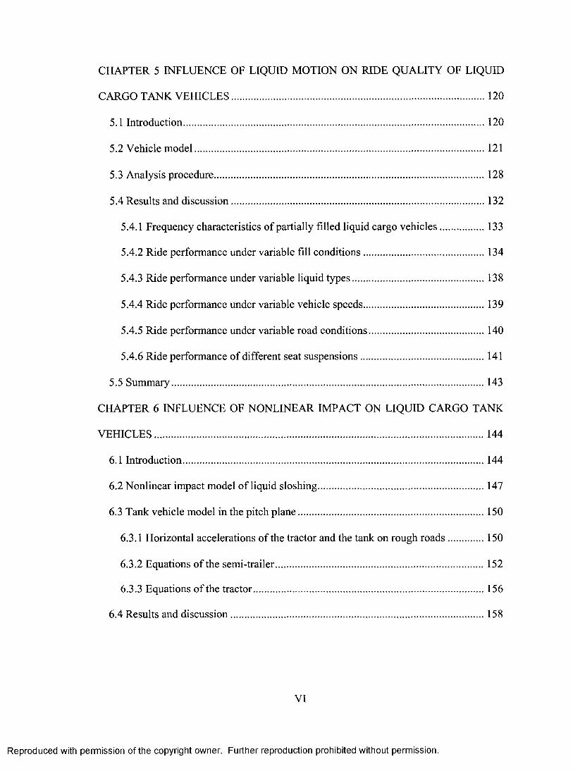
CHAPTER 5 INFLUENCE OF LIQUID MOTION ON RIDE QUALITY OF LIQUID
CARGO TANK VEHICLES 120
5.1 Introduction 120
5.2 Vehicle model 121
5.3 Analysis procedure 128
5.4 Results and discussion 132
5.4.1 Frequency characteristics of partially filled liquid cargo vehicles 133
5.4.2 Ride performance under variable fill conditions 134
5.4.3 Ride performance under variable liquid types 138
5.4.4 Ride performance under variable vehicle speeds 139
5.4.5 Ride performance under variable road conditions 140
5.4.6 Ride performance of different seat suspensions 141
5.5 Summary 143
CHAPTER 6 INFLUENCE OF NONLINEAR IMPACT ON LIQUID CARGO TANK
VEHICLES 144
6.1 Introduction 144
6.2 Nonlinear impact model of liquid sloshing 147
6.3 Tank vehicle model in the pitch plane 150
6.3.1 Horizontal accelerations of the tractor and the tank on rough roads 150
6.3.2 Equations of the semi-trailer 152
6.3.3 Equations of the tractor 156
6.4 Results and discussion 158
VI
Reproduced with permission of the copyright owner. Further reproduction prohibited without permission.
CHAPTER 5 INFLUENCE OF LIQUID MOTION ON RIDE QUALITY OF LIQUID
CARGO TANK VEHICLES...................................................................................................120
5.1 Introduction......................................................................................................................120
5.2 Vehicle m odel................................................................................................................. 121
5.3 Analysis procedure..........................................................................................................128
5.4 Results and discussion...................................................................................................132
5.4.1 Frequency characteristics o f partially filled liquid cargo vehicles.................. 133
5.4.2 Ride performance under variable fill conditions................................................134
5.4.3 Ride performance under variable liquid types.................................................... 138
5.4.4 Ride performance under variable vehicle speeds................................................139
5.4.5 Ride performance under variable road conditions..............................................140
5.4.6 Ride performance o f different seat suspensions.................................................141
5.5 Summary.......................................................................................................................... 143
CHAPTER 6 INFLUENCE OF NONLINEAR IMPACT ON LIQUID CARGO TANK
VEHICLES.................................................................................................................................144
6.1 Introduction......................................................................................................................144
6.2 Nonlinear impact model o f liquid sloshing................................................................. 147
6.3 Tank vehicle model in the pitch plane.........................................................................150
6.3.1 Horizontal accelerations of the tractor and the tank on rough roads...............150
6.3.2 Equations o f the semi-trailer..................................................................................152
6.3.3 Equations o f the tractor.......................................................................................... 156
6.4 Results and discussion................................................................................................... 158
VI
Reproduced with permission of the copyright owner. Further reproduction prohibited without permission.
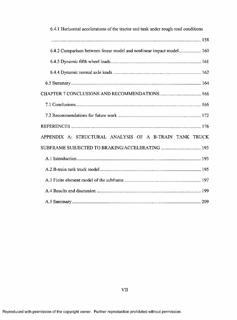
6.4.1 Horizontal accelerations of the tractor and tank under rough road conditions
158
6.4.2 Comparison between linear model and nonlinear impact model 160
6.4.3 Dynamic fifth wheel loads 161
6.4.4 Dynamic normal axle loads 162
6.5 Summary 164
CHAPTER 7 CONCLUSIONS AND RECOMMENDATIONS 166
7.1 Conclusions 166
7.2 Recommendations for future work 172
REFERENCES 176
APPENDIX A: STRUCTURAL ANALYSIS OF A B-TRAIN TANK TRUCK
SUBFRAME SUBJECTED TO BRAKING/ACCELERATING 193
A.1 Introduction 193
A.2 B-train tank truck model 195
A.3 Finite element model of the subframe 197
A.4 Results and discussion 199
A.5 Summary 209
VII
Reproduced with permission of the copyright owner. Further reproduction prohibited without permission.
6.4.1 Horizontal accelerations of the tractor and tank under rough road conditions
.............................................................................................................................................158
6.4.2 Comparison between linear model and nonlinear impact model..................... 160
6.4.3 Dynamic fifth wheel loads.....................................................................................161
6.4.4 Dynamic normal axle loads...................................................................................162
6.5 Summary........................................................................................................................ 164
CHAPTER 7 CONCLUSIONS AND RECOMMENDATIONS....................................... 166
7.1 Conclusions......................................................................................................................166
7.2 Recommendations for future w ork .............................................................................. 172
REFERENCES.......................................................................................................................... 176
APPENDIX A: STRUCTURAL ANALYSIS OF A B-TRAIN TANK TRUCK
SUBFRAME SUBJECTED TO BRAKING/ACCELERATING......................................193
A .l Introduction.....................................................................................................................193
A.2 B-train tank truck m odel...............................................................................................195
A.3 Finite element model of the subframe.........................................................................197
A.4 Results and discussion.................................................................................................. 199
A.5 Summary.........................................................................................................................209
VII
Reproduced with permission of the copyright owner. Further reproduction prohibited without permission.
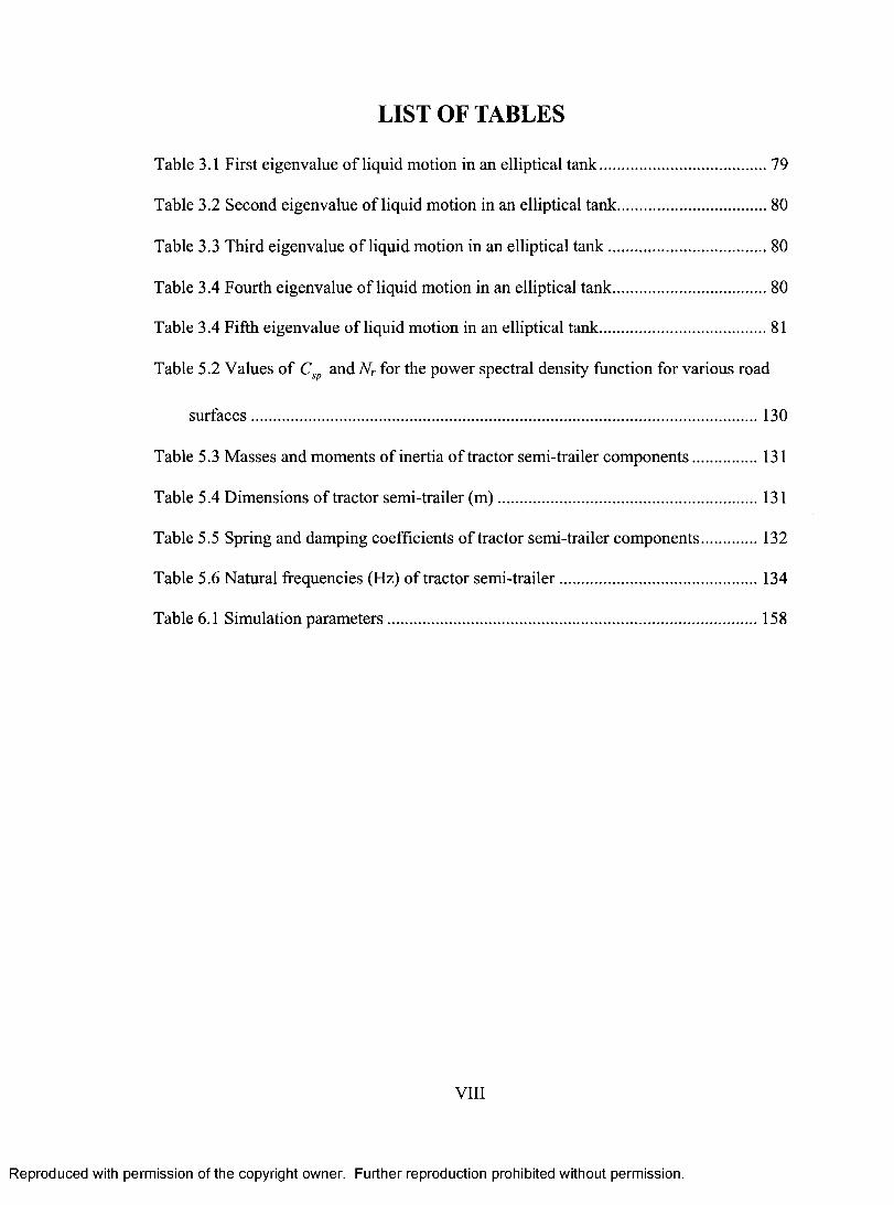
LIST OF TABLES
Table 3.1 First eigenvalue of liquid motion in an elliptical tank 79
Table 3.2 Second eigenvalue of liquid motion in an elliptical tank 80
Table 3.3 Third eigenvalue of liquid motion in an elliptical tank 80
Table 3.4 Fourth eigenvalue of liquid motion in an elliptical tank 80
Table 3.4 Fifth eigenvalue of liquid motion in an elliptical tank 81
Table 5.2 Values of C sp and N, for the power spectral density function for various road
surfaces 130
Table 5.3 Masses and moments of inertia of tractor semi-trailer components 131
Table 5.4 Dimensions of tractor semi-trailer (m) 131
Table 5.5 Spring and damping coefficients of tractor semi-trailer components 132
Table 5.6 Natural frequencies (Hz) of tractor semi-trailer 134
Table 6.1 Simulation parameters 158
VIII
Reproduced with permission of the copyright owner. Further reproduction prohibited without permission.
LIST OF TABLES
Table 3.1 First eigenvalue o f liquid motion in an elliptical tank.......................................... 79
Table 3.2 Second eigenvalue o f liquid motion in an elliptical tank......................................80
Table 3.3 Third eigenvalue o f liquid motion in an elliptical tan k ........................................80
Table 3.4 Fourth eigenvalue of liquid motion in an elliptical tank.......................................80
Table 3.4 Fifth eigenvalue of liquid motion in an elliptical tank.......................................... 81
Table 5.2 Values o f Csp and Nr for the power spectral density function for various road
surfaces.............................................................................................................................. 130
Table 5.3 Masses and moments o f inertia o f tractor semi-trailer components................. 131
Table 5.4 Dimensions of tractor semi-trailer (m )................................................................. 131
Table 5.5 Spring and damping coefficients of tractor semi-trailer components...............132
Table 5.6 Natural frequencies (Hz) of tractor semi-trailer.................................................. 134
Table 6.1 Simulation parameters.............................................................................................158
VIII
Reproduced with permission of the copyright owner. Further reproduction prohibited without permission.
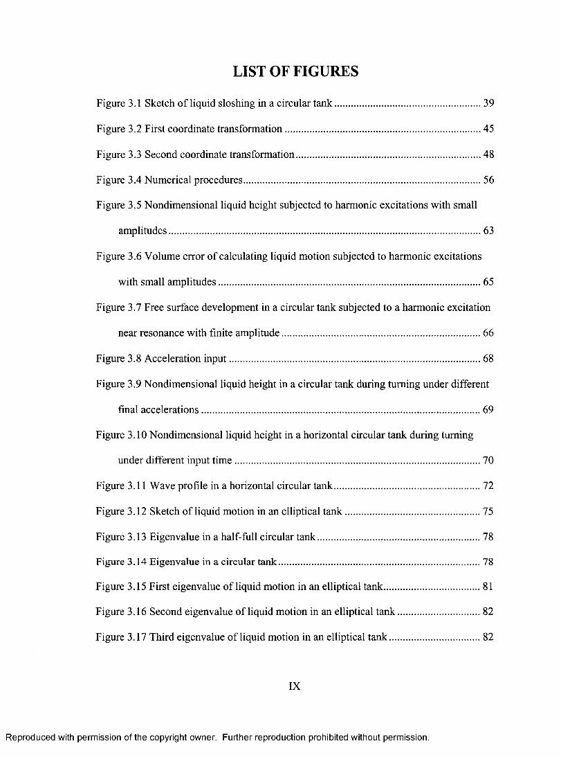
LIST OF FIGURES
Figure 3.1 Sketch of liquid sloshing in a circular tank 39
Figure 3.2 First coordinate transformation 45
Figure 3.3 Second coordinate transformation 48
Figure 3.4 Numerical procedures 56
Figure 3.5 Nondimensional liquid height subjected to harmonic excitations with small
amplitudes 63
Figure 3.6 Volume error of calculating liquid motion subjected to harmonic excitations
with small amplitudes 65
Figure 3.7 Free surface development in a circular tank subjected to a harmonic excitation
near resonance with finite amplitude 66
Figure 3.8 Acceleration input 68
Figure 3.9 Nondimensional liquid height in a circular tank during turning under different
final accelerations 69
Figure 3.10 Nondimensional liquid height in a horizontal circular tank during turning
under different input time 70
Figure 3.11 Wave profile in a horizontal circular tank 72
Figure 3.12 Sketch of liquid motion in an elliptical tank 75
Figure 3.13 Eigenvalue in a half-full circular tank 78
Figure 3.14 Eigenvalue in a circular tank 78
Figure 3.15 First eigenvalue of liquid motion in an elliptical tank 81
Figure 3.16 Second eigenvalue of liquid motion in an elliptical tank 82
Figure 3.17 Third eigenvalue of liquid motion in an elliptical tank 82
IX
Reproduced with permission of the copyright owner. Further reproduction prohibited without permission.
LIST OF FIGURES
Figure 3.1 Sketch of liquid sloshing in a circular tank .......................................................... 39
Figure 3.2 First coordinate transformation..............................................................................45
Figure 3.3 Second coordinate transformation..........................................................................48
Figure 3.4 Numerical procedures.............................................................................................. 56
Figure 3.5 Nondimensional liquid height subjected to harmonic excitations with small
amplitudes............................................................................................................................63
Figure 3.6 Volume error of calculating liquid motion subjected to harmonic excitations
with small amplitudes........................................................................................................ 65
Figure 3.7 Free surface development in a circular tank subjected to a harmonic excitation
near resonance with finite amplitude............................................................................... 6 6
Figure 3.8 Acceleration input....................................................................................................6 8
Figure 3.9 Nondimensional liquid height in a circular tank during turning under different
final accelerations...............................................................................................................69
Figure 3.10 Nondimensional liquid height in a horizontal circular tank during turning
under different input tim e ..................................................................................................70
Figure 3.11 Wave profile in a horizontal circular tank.......................................................... 72
Figure 3.12 Sketch of liquid motion in an elliptical tan k ......................................................75
Figure 3.13 Eigenvalue in a half-full circular tank.................................................................78
Figure 3.14 Eigenvalue in a circular tank........................................................................................ 78
Figure 3.15 First eigenvalue o f liquid motion in an elliptical tank.......................................81
Figure 3.16 Second eigenvalue of liquid motion in an elliptical tank ................................. 82
Figure 3.17 Third eigenvalue o f liquid motion in an elliptical tank .....................................82
IX
Reproduced with permission of the copyright owner. Further reproduction prohibited without permission.
Figure 3.18 Fourth eigenvalue of liquid motion in an elliptical tank 83
Figure 3.19 Fifth eigenvalue of liquid motion in an elliptical tank 83
Figure 4.1 Sketch of horizontal cylindrical tanks 89
Figure 4.2 First eigenvalue in the longitudinal direction for liquid motion in a cylindrical
tank 106
Figure 4.3 Force and moment calculation by fluid dynamics 107
Figure 4.4 Force and moment calculation by mass centre 107
Figure 4.5 Force and moment under different accelerations 109
Figure 4.6 Free surface development under different accelerations 110
Figure 4.7 Force and moment under different fill levels 112
Figure 4.8 Force and moment for different tank shapes 113
Figure 4.9 Free surface development in a tank with hemispherical heads 113
Figure 4.10 Axial forces in compartmented tanks 117
Figure 4.11 Influence of input time 115
Figure 5.1 Pitch plane model of the tractor semi-trailer 124
Figure 5.2 Influence of variable fill levels (20%) 135
Figure 5.3 Influence of variable fill levels (50%) 136
Figure 5.4 Influence of variable fill levels (80%) 137
Figure 5.5 Influence of liquid densities 139
Figure 5.6 Influence of vehicle speed 140
Figure 5.7 Influence of road condition 141
Figure 5.8 Influence of seat suspension 142
Figure 6.1 Tractor semi-trailer model and motion profile 150
X
Reproduced with permission of the copyright owner. Further reproduction prohibited without permission.
Figure 3.18 Fourth eigenvalue of liquid motion in an elliptical tan k .................................. 83
Figure 3.19 Fifth eigenvalue of liquid motion in an elliptical tan k ......................................83
Figure 4.1 Sketch of horizontal cylindrical tanks................................................................... 89
Figure 4.2 First eigenvalue in the longitudinal direction for liquid motion in a cylindrical
tank...................................................................................................................................... 106
Figure 4.3 Force and moment calculation by fluid dynamics.............................................. 107
Figure 4.4 Force and moment calculation by mass centre................................................. 107
Figure 4.5 Force and moment under different accelerations...............................................109
Figure 4.6 Free surface development under different accelerations...................................110
Figure 4.7 Force and moment under different fill levels..................................................... 112
Figure 4.8 Force and moment for different tank shapes...................................................... 113
Figure 4.9 Free surface development in a tank with hemispherical heads........................113
Figure 4.10 Axial forces in compartmented tanks................................................................ 117
Figure 4.11 Influence of input tim e........................................................................................ 115
Figure 5.1 Pitch plane model of the tractor semi-trailer...................................................... 124
Figure 5.2 Influence o f variable fill levels (20%)................................................................. 135
Figure 5.3 Influence of variable fill levels (50%)................................................................. 136
Figure 5.4 Influence o f variable fill levels (80%)................................................................. 137
Figure 5.5 Influence o f liquid densities..................................................................................139
Figure 5.6 Influence o f vehicle speed.....................................................................................140
Figure 5.7 Influence o f road condition...................................................................................141
Figure 5.8 Influence o f seat suspension..................................................................................142
Figure 6.1 Tractor semi-trailer model and motion profile................................................... 150
X
Reproduced with permission of the copyright owner. Further reproduction prohibited without permission.
Figure 6.2 Loading configuration of the semi-trailer 154
Figure 6.3 Loading configuration of the tractor 156
Figure 6.4 Horizontal accelerations of the tractor and tank 159
Figure 6.5 Nondimensional sloshing mass displacement (wavelength: 75m) 160
Figure 6.6 Nondimensional sloshing mass displacement (wavelength: 100m) 161
Figure 6.7 Fifth wheel loads 163
Figure 6.8 Normal axle loads 164
Figure A.1 Schematic of a B-train tank truck 196
Figure A.2 Subframe model 198
Figure A.3 Load shift during acceleration 200
Figure A.4 Load shift during braking 201
Figure A.5 Forces at hitch point during acceleration 202
Figure A.6 Forces at hitch point during braking 203
Figure A.7 Force difference between the liquid cargo and equivalent rigid cargo 204
Figure A.8 Stress distributions of the subframe 206
Figure A.9 Von Mises stress at critical node 208
XI
Reproduced with permission of the copyright owner. Further reproduction prohibited without permission.
Figure 6.2 Loading configuration of the semi-trailer............................................................154
Figure 6.3 Loading configuration o f the tractor.....................................................................156
Figure 6.4 Horizontal accelerations o f the tractor and tank.................................................159
Figure 6.5 Nondimensional sloshing mass displacement (wavelength: 75m ).................. 160
Figure 6 .6 Nondimensional sloshing mass displacement (wavelength: 100m)................161
Figure 6.7 Fifth wheel loads.................................................................................................... 163
Figure 6 .8 Normal axle loads................................................................................................... 164
Figure A. 1 Schematic o f a B-train tank truck.......................................................................196
Figure A.2 Subframe model..................................................................................................... 198
Figure A.3 Load shift during acceleration.............................................................................200
Figure A.4 Load shift during braking.....................................................................................201
Figure A.5 Forces at hitch point during acceleration........................................................... 202
Figure A .6 Forces at hitch point during braking...................................................................203
Figure A.7 Force difference between the liquid cargo and equivalent rigid cargo 204
Figure A .8 Stress distributions of the subframe.................................................................... 206
Figure A.9 Von Mises stress at critical node.........................................................................208
XI
Reproduced with permission of the copyright owner. Further reproduction prohibited without permission.
NOMENCLATURE
a: half of the major axis length of elliptical tanks
al , a2 , a3, a30 , a4 , ael , ae2 , a , 3 , ae4 , as : geometric parameters of tractor semi-trailer
aft: horizontal acceleration of the tractor in the local coordinate system
an : amplitude of the road contour
art: horizontal acceleration of the tank in the local coordinate system
at: applied acceleration on the equivalent mass
A,B,C,D,E,F,G: parameters used in calculation
Ao: final acceleration value when applied by a ramp function
Ag, Bg: parameter for adjusting the grid clustering
At, Az: lateral and longitudinal accelerations applied on the liquid
b: half of the minor axis length of elliptical tanks
,b5 : geometric parameters of tractor semi-trailer
bn : positive constant impact parameter
B: parameter for adjusting the grid clustering
Bir, B2r: coefficient matrices
B, G,, Ei, Di, Ii, Hi: coefficients used in the transformations
C:
CO:
elf :
e l2 :
half length of horizontal cylindrical tanks with flat heads
and half length of cylindrical section of tanks with hemispherical heads
distance between the still liquid surface and the coordinate system origin
damping coefficient of the tractor front suspension
damping coefficient of the tractor rear suspension
XII
Reproduced with permission of the copyright owner. Further reproduction prohibited without permission.
NOMENCLATURE
a: half of the major axis length of elliptical tanks
ax,a 2,a 2, ai0, a4, aei, ae2, aei, ae4, as : geometric parameters o f tractor semi-trailer
a/x: horizontal acceleration o f the tractor in the local coordinate system
a„ : amplitude of the road contour
arx'. horizontal acceleration of the tank in the local coordinate system
ax: applied acceleration on the equivalent mass
A ,B ,C ,D ,E ,F ,G : parameters used in calculation
Ao: final acceleration value when applied by a ramp function
Ag, Bg. parameter for adjusting the grid clustering
AXf Az: lateral and longitudinal accelerations applied on the liquid
b : half o f the minor axis length of elliptical tanks
b{, b20, b4, bs : geometric parameters of tractor semi-trailer
bn : positive constant impact parameter
B\ parameter for adjusting the grid clustering
B\r, B2/. coefficient matrices
Bj Gj Ejf Df Ii Hf. coefficients used in the transformations
c : half length of horizontal cylindrical tanks with flat heads
and half length of cylindrical section of tanks with hemispherical heads
co: distance between the still liquid surface and the coordinate system origin
cn : damping coefficient o f the tractor front suspension
c, 2 : damping coefficient of the tractor rear suspension
XII
Reproduced with permission of the copyright owner. Further reproduction prohibited without permission.
C21 :
Cf.
Cni:
C,:
C,11
C,12
Cal
damping coefficient of the semi-trailer suspension
artificial damping coefficient
equivalent damping coefficient of the equivalent mass-spring system
damping coefficient of the seat
damping coefficient of the tractor front axle
damping coefficient of the tractor rear axle
damping coefficient of the semi-trailer axle
Ci coefficients used in the transformations
Cr:
d:
D:
Do:
f f :
f.:
f
Fd:
F m:
F1• •
Fim:
damping matrix
constant for the road surface
still liquid height
tank diameter
amplitude of the tank displacement
tank displacement
frequency in the unit of Hz
tractor front axle rolling resistance coefficient
tractor rear axle rolling resistance coefficient
semi-trailer axle rolling resistance coefficient
driving force
tractor rear axle normal force
tractor front axle normal force
impact force
XIII
Reproduced with permission of the copyright owner. Further reproduction prohibited without permission.
c21: damping coefficient of the semi-trailer suspension
cf. artificial damping coefficient
cn\: equivalent damping coefficient o f the equivalent mass-spring system
cs : damping coefficient of the seat
clU : damping coefficient o f the tractor front axle
c, 12 : damping coefficient o f the tractor rear axle
cm : damping coefficient of the semi-trailer axle
Ci K if J if Mi, Liw Nf. coefficients used in the transformations
C,: damping matrix
Cv - constant for the road surface
d: still liquid height
D: tank diameter
Do: amplitude o f the tank displacement
Dx: tank displacement
f i frequency in the unit of Hz
fr tractor front axle rolling resistance coefficient
fm- tractor rear axle rolling resistance coefficient
fr - semi-trailer axle rolling resistance coefficient
Fd: driving force
Fm: tractor rear axle normal force
Fr tractor front axle normal force
F ■1 im• impact force
XIII
Reproduced with permission of the copyright owner. Further reproduction prohibited without permission.
FL:
Fr :
Frp
Fx :
Fy :
FZ :
g:
Gy:
h:
H:
H:
H*:
He:
force vector caused by liquid motion
liquid fill level
semi-trailer axle normal force
Laplace transform vector
interaction force between the liquid and the tank walls
horizontal force in the global coordinate system on the fifth wheel
vertical force in the global coordinate system on the fifth wheel
longitudinal liquid force
acceleration due to gravitation
frequency response of a given output yr in response to the road input
dynamic liquid height in the transformed coordinate system
dynamic liquid height in the transformed coordinate system
smoothed dynamic liquid height in the transformed coordinate system
dynamic liquid height in the transformed coordinate system
equivalent still liquid height
hoi,h1,, h2,14, H1,H2: geometric parameters of the tractor semi-trailer
j, k:
/ 20
I rl •
k11 :
k12 :
indices
moment of inertia of the empty semi-trailer
moment of inertia of the tractor
combined moment of inertia of semi-trailer and all fixed parts of the liquid
spring coefficient of the tractor front suspension
spring coefficient of the tractor rear suspension
XIV
Reproduced with permission of the copyright owner. Further reproduction prohibited without permission.
F[ : force vector caused by liquid motion
FL: liquid fill level
Fr : semi-trailer axle normal force
Frp: Laplace transform vector
Fs\ interaction force between the liquid and the tank walls
Fx : horizontal force in the global coordinate system on the fifth wheel
Fy : vertical force in the global coordinate system on the fifth wheel
F : longitudinal liquid force
g: acceleration due to gravitation
Gy. frequency response o f a given output jv in response to the road input
h: dynamic liquid height in the transformed coordinate system
H: dynamic liquid height in the transformed coordinate system
H : smoothed dynamic liquid height in the transformed coordinate system
F t : dynamic liquid height in the transformed coordinate system
He\ equivalent still liquid height
Aoy, hy, li2,hw, H\,H 2 '. geometric parameters o f the tractor semi-trailer
i,j, k: indices
I 20: moment o f inertia o f the empty semi-trailer
I rt: moment o f inertia o f the tractor
I r2: combined moment o f inertia o f semi-trailer and all fixed parts o f the liquid
ki,: spring coefficient of the tractor front suspension
kn : spring coefficient o f the tractor rear suspension
XIV
Reproduced with permission of the copyright owner. Further reproduction prohibited without permission.
k 21
kf
kg:
kil:
k :
k t 1 1 :
k t 12 :
k t 21 :
1, :
L:
Le:
LI :
m20 • '
ml:
Mnl
mri
M r2
ms :
spring coefficient of the semi-trailer suspension
artificial soft spring coefficient
parameter for adjusting the grid clustering
equivalent stiffness coefficient of the equivalent mass-spring system
spring coefficient of the seat
spring coefficient of the tractor front axle
spring coefficient of the tractor rear axle
spring coefficient of the semi-trailer axle
stiffness matrices
L,„: geometric parameters of the tractor semi-trailer
distance from the still free surface to the centre of fixed mass
distance from the still free surface to the centre of sloshing mass
distance between the tractor rear axle and semi-trailer axle
Lagrangian
equivalent tank length
distance between the tractor front axle and tractor rear axle
mass of the empty semi-trailer
total liquid mass inside the tank
equivalent mass of the equivalent mass-spring system
mass of the tractor
combined mass of the empty semi-trailer and all fixed parts of the liquid
mass of the seat and the driver
XV
Reproduced with permission of the copyright owner. Further reproduction prohibited without permission.
k2l: spring coefficient o f the semi-trailer suspension
kf. artificial soft spring coefficient
kg. parameter for adjusting the grid clustering
kn\. equivalent stiffness coefficient o f the equivalent mass-spring system
ks - spring coefficient o f the seat
k, 11 • spring coefficient o f the tractor front axle
kt 12 • spring coefficient of the tractor rear axle
kt 21. spring coefficient of the semi-trailer axle
Kr. stiffness matrices
Ij, kjt lg> Av, k w. geometric parameters of the tractor semi-trailer
1/nO '• distance from the still free surface to the centre of fixed mass
AbI '• distance from the still free surface to the centre o f sloshing mass
k- distance between the tractor rear axle and semi-trailer axle
L : Lagrangian
Le: equivalent tank length
V distance between the tractor front axle and tractor rear axle
m2o : mass o f the empty semi-trailer
mi: total liquid mass inside the tank
m„ i : equivalent mass of the equivalent mass-spring system
mrX\ mass of the tractor
mr2: combined mass o f the empty semi-trailer and all fixed parts o f the liq
ms : mass o f the seat and the driver
XV
Reproduced with permission of the copyright owner. Further reproduction prohibited without permission.
mill mass of the tractor front axle
Mt12 : mass of the tractor rear axle
Mt21 mass of the semi-trailer axle
MI : moment caused by liquid motion
/1-;/, : moment vector caused by liquid motion
Mr: mass matrix
n: normal direction on the curved walls
nn : positive impact integer
N, M, L: total numbers of cells in x*,Y* and Z* directions
Nn: number of compartments
Nr : constant for the road surface
P: liquid pressure
Q,: jth generalized force
R: radius of the cylindrical tank
Rf •• tractor front axle rolling resistance
R„, : tractor rear axle rolling resistance
Rr : semi-trailer axle rolling resistance
Re: Reynolds number
S: cross-section area of the liquid in the cylindrical section
Sy : power spectral density of a given output variable
S zii : power spectral density function of the elevation of the road surface profile
t: time
XVI
Reproduced with permission of the copyright owner. Further reproduction prohibited without permission.
m ,u : mass o f the tractor front axle
mt\2 • mass o f the tractor rear axle
m, 21: mass o f the semi-trailer axle
M r. moment caused by liquid motion
Mr- moment vector caused by liquid motion
Mr\ mass matrix
n: normal direction on the curved walls
n„ : positive impact integer
N, M, L: total numbers o f cells in X*, Y* and Z* directions
Nn: number of compartments
Nr : constant for the road surface
P- liquid pressure
Qrr yth generalized force
R : radius of the cylindrical tank
Rf : tractor front axle rolling resistance
Rm- tractor rear axle rolling resistance
K - semi-trailer axle rolling resistance
Re: Reynolds number
S: cross-section area of the liquid in the cylindrical section
Sy : power spectral density o f a given output variable
•• power spectral density function o f the elevation o f the road surface profile
t: time
XVI
Reproduced with permission of the copyright owner. Further reproduction prohibited without permission.

to: acceleration input time when applied by a ramp function
: delay time for the tractor rear axle
12 : delay time for the semi-trailer axle
ur: horizontal velocity of the tank in the local coordinate system
Uf : horizontal velocity of the tractor in the global coordinate system
horizontal velocity in the global coordinate system
Ur: horizontal velocity of the tank in the global coordinate system
Urp: vector of instantaneous values of vertical displacements of the road profile
at each axle location
v: speed of the vehicle
of vertical velocity of the tractor in the local coordinate system
vr: vertical velocity of the tank in the local coordinate system
V: liquid volume in the hemispherical head
Vj vertical velocity of the tractor in the global coordinate system
Vn: vertical velocity in the global coordinate system
Vr: vertical velocity of the tank in the global coordinate system
w: longitudinal length of the tank compartment
weight of the jth fixed mass
Wif • weight of the jth sloshing mass •
coefficients used in the transformations
W k : weight of the tractor
WL: wavelength of the road contour
XVII
Reproduced with permission of the copyright owner. Further reproduction prohibited without permission.
t0: acceleration input time when applied by a ramp function
t{: delay time for the tractor rear axle
t2: delay time for the semi-trailer axle
ur'. horizontal velocity o f the tank in the local coordinate system
U f: horizontal velocity o f the tractor in the global coordinate system
U„: horizontal velocity in the global coordinate system
Ur: horizontal velocity o f the tank in the global coordinate system
Urp. vector of instantaneous values of vertical displacements o f the road profile
at each axle location
v: speed of the vehicle
v/. vertical velocity of the tractor in the local coordinate system
vr: vertical velocity of the tank in the local coordinate system
V: liquid volume in the hemispherical head
V/. vertical velocity of the tractor in the global coordinate system
Vn: vertical velocity in the global coordinate system
Vr\ vertical velocity o f the tank in the global coordinate system
w: longitudinal length of the tank compartment
W0 j : weight of they'th fixed mass
Wyj : weight o f the yth sloshing mass
Wi Pi, Oi Si, Qi, Ri. coefficients used in the transformations
Wk : weight o f the tractor
WL: wavelength of the road contour
XVII
Reproduced with permission of the copyright owner. Further reproduction prohibited without permission.
W:
x, y, z:
x1,y1,z1:
xc :
xej:
xn, yn:
Xn0
Xr 1 :
Xr2:
Xs:
Xill:
Xt 1 2:
Xt21:
X, Y, Z:
Y Z :
Xfi
X., Y.:
Xn, Yn:
Xr, Yr:
Yr;
Yrp:
weight of the empty semi-trailer
coordinate system for coordinate transformation
coordinates for liquid sloshing inside tanks
nondimensional displacement
horizontal displacement of jth sloshing mass
local coordinate system on the tractor and the tank
displacement when the equivalent mass reaches the compartment walls
horizontal displacement of the tractor mass centre
Horizontal displacement of the semi-trailer mass centre
horizontal displacement of the seat
horizontal displacement of the tractor front axle
horizontal displacement of the tractor rear axle
horizontal displacement of the semi-trailer axle
coordinate system for coordinate transformation
coordinate system for coordinate transformation
global coordinates of tractor front tire-ground contact point
global coordinates of tractor rear tire-ground contact points
global coordinates of the tractor semi-trailer
global coordinates of semi-trailer tire-ground contact points
jth generalized coordinate of the vehicle system
vertical and longitudinal distances between the mass centre and
the selected axis for moment calculation
independent generalized coordinate vector
XVIII
Reproduced with permission of the copyright owner. Further reproduction prohibited without permission.
Wt : weight of the empty semi-trailer
x, y, z: coordinate system for coordinate transformation
jcijyz,: coordinates for liquid sloshing inside tanks
x c : nondimensional displacement
xej\ horizontal displacement ofy'th sloshing mass
x„, y„: local coordinate system on the tractor and the tank
x„o: displacement when the equivalent mass reaches the compartment walls
xr\: horizontal displacement of the tractor mass centre
xry. Horizontal displacement of the semi-trailer mass centre
Xyi horizontal displacement of the seat
xt\\\ horizontal displacement of the tractor front axle
xtn- horizontal displacement of the tractor rear axle
xa\. horizontal displacement of the semi-trailer axle
X, Y, Z: coordinate system for coordinate transformation
X*, Y*, Z*\ coordinate system for coordinate transformation
Xf, Yf. global coordinates of tractor front tire-ground contact point
X m, Ym: global coordinates o f tractor rear tire-ground contact points
X„, Yn: global coordinates o f the tractor semi-trailer
X r, Yr: global coordinates of semi-trailer tire-ground contact points
y rJ : yth generalized coordinate o f the vehicle system
y x, Zj: vertical and longitudinal distances between the mass centre and
the selected axis for moment calculation
Yrp\ independent generalized coordinate vector
XVIII
Reproduced with permission of the copyright owner. Further reproduction prohibited without permission.
Z11:
Z12:
Z21:
Zej:
Zrl:
Zr2:
Zs:
Ztll:
Zt12:
Z121:
a,13, y:
an, fin:
x:
8:
(1):
17:
17n:
f:
corn:
cor:
K:
road profile at the tractor front axle
road profile at the tractor rear axle
road profile at the semi-trailer axle
vertical displacement of jth sloshing mass
vertical displacement of the tractor mass centre
vertical displacement of the semi-trailer mass centre
vertical displacement of the seat
vertical displacement of the tractor front axle
vertical displacement of the tractor rear axle
vertical displacement of the semi-trailer axle
coordinate system for coordinate transformation
angle of the tank with respect to the X„ and Y, coordinates
eigenvector
parameter for different tank head types
velocity potential in the transformed coordinate system
free surface elevation in the transformed coordinate system
positive impact integer
velocity potential in the original coordinate system
road profile tangent angle at tire-ground contact point of tractor front axle
road profile tangent angle at tire-ground contact point of tractor rear axle
road profile tangent angle at tire-ground contact point of semi-trailer axle
eigenvalue
XIX
Reproduced with permission of the copyright owner. Further reproduction prohibited without permission.
z 1 1 : road profile at the tractor front axle
z\2 '. road profile at the tractor rear axle
Z2 \: road profile at the semi-trailer axle
zef. vertical displacement ofy'th sloshing mass
zr\: vertical displacement o f the tractor mass centre
z r2 '■ vertical displacement of the semi-trailer mass centre
zv: vertical displacement o f the seat
zt11: vertical displacement of the tractor front axle
zt\2- vertical displacement of the tractor rear axle
za\. vertical displacement of the semi-trailer axle
a, p, y: coordinate system for coordinate transformation
an p n\ angle o f the tank with respect to the X„ and Yn coordinates
X '■ eigenvector
8 : parameter for different tank head types
<p. velocity potential in the transformed coordinate system
77: free surface elevation in the transformed coordinate system
T]n: positive impact integer
qr. velocity potential in the original coordinate system
<pf : road profile tangent angle at tire-ground contact point o f tractor front axle
(pm: road profile tangent angle at tire-ground contact point o f tractor rear axle
cpr : road profile tangent angle at tire-ground contact point o f semi-trailer axle
k : eigenvalue
XIX
Reproduced with permission of the copyright owner. Further reproduction prohibited without permission.
ith eigenvalue
p: damping coefficient in the modified Rayleigh term
7r 3.1415926
A free surface angle when liquid motion modeled by mass centre models
01: angular displacement of the tractor
02: angular displacement of the semi-trailer
0„ : pendulum angular displacement
0„n : angular displacement when the pendulum reached the container walls
P: liquid density
co: excitation frequency
co,: natural frequency of liquid motion
con: first liquid sloshing frequency
free surface elevation above still liquid level in xiy,z, coordinate system
nondimensional damping coefficient
0: velocity potential in the transformed coordinate system
velocity potential in the transformed coordinate system
II : impact potential energy function
O : coefficient matrix in the eigenvalue problem
: spatial frequency
: coefficient matrix in the eigenvalue problem
XX
Reproduced with permission of the copyright owner. Further reproduction prohibited without permission.
X{. ith eigenvalue
ji\ damping coefficient in the modified Rayleigh term
tv. 3.1415926
&. free surface angle when liquid motion modeled by mass centre models
9\ : angular displacement o f the tractor
6 2 ' angular displacement o f the semi-trailer
dn: pendulum angular displacement
0 nQ: angular displacement when the pendulum reached the container walls
p\ liquid density
co\ excitation frequency
C0i\ natural frequency o f liquid motion
con: first liquid sloshing frequency
free surface elevation above still liquid level in x xy xz x coordinate system
Q. nondimensional damping coefficient
d>. velocity potential in the transformed coordinate system
0 *: velocity potential in the transformed coordinate system
1 1 : impact potential energy function
0 : coefficient matrix in the eigenvalue problem
Q : spatial frequency
W : coefficient matrix in the eigenvalue problem
XX
Reproduced with permission of the copyright owner. Further reproduction prohibited without permission.
CHAPTER 1 INTRODUCTION
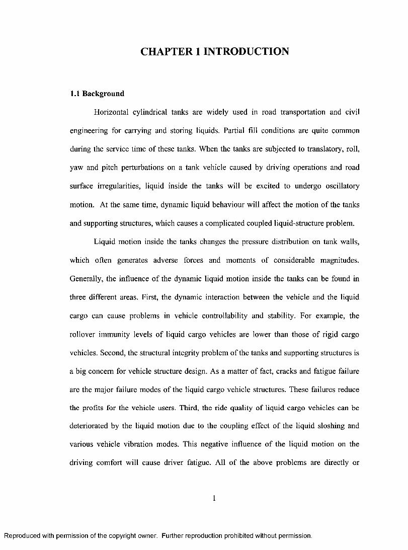
1.1 Background
Horizontal cylindrical tanks are widely used in road transportation and civil
engineering for carrying and storing liquids. Partial fill conditions are quite common
during the service time of these tanks. When the tanks are subjected to translatory, roll,
yaw and pitch perturbations on a tank vehicle caused by driving operations and road
surface irregularities, liquid inside the tanks will be excited to undergo oscillatory
motion. At the same time, dynamic liquid behaviour will affect the motion of the tanks
and supporting structures, which causes a complicated coupled liquid-structure problem.
Liquid motion inside the tanks changes the pressure distribution on tank walls,
which often generates adverse forces and moments of considerable magnitudes.
Generally, the influence of the dynamic liquid motion inside the tanks can be found in
three different areas. First, the dynamic interaction between the vehicle and the liquid
cargo can cause problems in vehicle controllability and stability. For example, the
rollover immunity levels of liquid cargo vehicles are lower than those of rigid cargo
vehicles. Second, the structural integrity problem of the tanks and supporting structures is
a big concern for vehicle structure design. As a matter of fact, cracks and fatigue failure
are the major failure modes of the liquid cargo vehicle structures. These failures reduce
the profits for the vehicle users. Third, the ride quality of liquid cargo vehicles can be
deteriorated by the liquid motion due to the coupling effect of the liquid sloshing and
various vehicle vibration modes. This negative influence of the liquid motion on the
driving comfort will cause driver fatigue. All of the above problems are directly or
1
Reproduced with permission of the copyright owner. Further reproduction prohibited without permission.
CHAPTER 1 INTRODUCTION
1.1 Background
Horizontal cylindrical tanks are widely used in road transportation and civil
engineering for carrying and storing liquids. Partial fill conditions are quite common
during the service time o f these tanks. When the tanks are subjected to translatory, roll,
yaw and pitch perturbations on a tank vehicle caused by driving operations and road
surface irregularities, liquid inside the tanks will be excited to undergo oscillatory
motion. At the same time, dynamic liquid behaviour will affect the motion o f the tanks
and supporting structures, which causes a complicated coupled liquid-structure problem.
Liquid motion inside the tanks changes the pressure distribution on tank walls,
which often generates adverse forces and moments of considerable magnitudes.
Generally, the influence of the dynamic liquid motion inside the tanks can be found in
three different areas. First, the dynamic interaction between the vehicle and the liquid
cargo can cause problems in vehicle controllability and stability. For example, the
rollover immunity levels o f liquid cargo vehicles are lower than those o f rigid cargo
vehicles. Second, the structural integrity problem of the tanks and supporting structures is
a big concern for vehicle structure design. As a matter o f fact, cracks and fatigue failure
are the major failure modes o f the liquid cargo vehicle structures. These failures reduce
the profits for the vehicle users. Third, the ride quality o f liquid cargo vehicles can be
deteriorated by the liquid motion due to the coupling effect o f the liquid sloshing and
various vehicle vibration modes. This negative influence o f the liquid motion on the
driving comfort will cause driver fatigue. All o f the above problems are directly or
1
Reproduced with permission of the copyright owner. Further reproduction prohibited without permission.
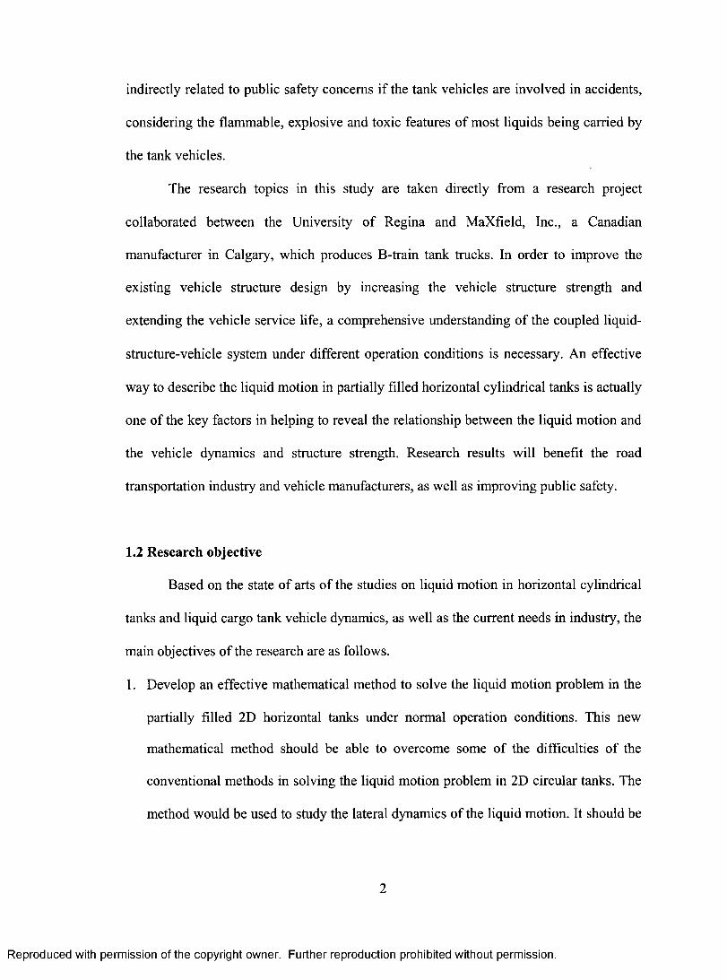
indirectly related to public safety concerns if the tank vehicles are involved in accidents,
considering the flammable, explosive and toxic features of most liquids being carried by
the tank vehicles.
The research topics in this study are taken directly from a research project
collaborated between the University of Regina and MaXfield, Inc., a Canadian
manufacturer in Calgary, which produces B-train tank trucks. In order to improve the
existing vehicle structure design by increasing the vehicle structure strength and
extending the vehicle service life, a comprehensive understanding of the coupled liquid-
structure-vehicle system under different operation conditions is necessary. An effective
way to describe the liquid motion in partially filled horizontal cylindrical tanks is actually
one of the key factors in helping to reveal the relationship between the liquid motion and
the vehicle dynamics and structure strength. Research results will benefit the road
transportation industry and vehicle manufacturers, as well as improving public safety.
1.2 Research objective
Based on the state of arts of the studies on liquid motion in horizontal cylindrical
tanks and liquid cargo tank vehicle dynamics, as well as the current needs in industry, the
main objectives of the research are as follows.
1. Develop an effective mathematical method to solve the liquid motion problem in the
partially filled 2D horizontal tanks under normal operation conditions. This new
mathematical method should be able to overcome some of the difficulties of the
conventional methods in solving the liquid motion problem in 2D circular tanks. The
method would be used to study the lateral dynamics of the liquid motion. It should be
2
Reproduced with permission of the copyright owner. Further reproduction prohibited without permission.
indirectly related to public safety concerns if the tank vehicles are involved in accidents,
considering the flammable, explosive and toxic features of most liquids being carried by
the tank vehicles.
The research topics in this study are taken directly from a research project
collaborated between the University o f Regina and MaXfield, Inc., a Canadian
manufacturer in Calgary, which produces B-train tank trucks. In order to improve the
existing vehicle structure design by increasing the vehicle structure strength and
extending the vehicle service life, a comprehensive understanding of the coupled liquid-
structure-vehicle system under different operation conditions is necessary. An effective
way to describe the liquid motion in partially filled horizontal cylindrical tanks is actually
one of the key factors in helping to reveal the relationship between the liquid motion and
the vehicle dynamics and structure strength. Research results will benefit the road
transportation industry and vehicle manufacturers, as well as improving public safety.
1.2 Research objective
Based on the state o f arts o f the studies on liquid motion in horizontal cylindrical
tanks and liquid cargo tank vehicle dynamics, as well as the current needs in industry, the
main objectives o f the research are as follows.
1. Develop an effective mathematical method to solve the liquid motion problem in the
partially filled 2D horizontal tanks under normal operation conditions. This new
mathematical method should be able to overcome some o f the difficulties of the
conventional methods in solving the liquid motion problem in 2D circular tanks. The
method would be used to study the lateral dynamics o f the liquid motion. It should be
2
Reproduced with permission of the copyright owner. Further reproduction prohibited without permission.
easy to apply to tanks of other shapes, such as elliptical tanks. It should also be easy
to extend the method to solve liquid motion problems in 3D horizontal cylindrical
tanks.
2. Develop an effective mathematical method to solve the liquid motion in the partially
filled 3D horizontal cylindrical tanks under normal operation conditions. This
situation had seldom been studied in the liquid cargo vehicle dynamics due to the lack
of an effective algorithm to describe the liquid motion in horizontal cylindrical tanks
in a completely 3D manner. The method should be able to be used to study the
longitudinal liquid dynamics, as well as the combined longitudinal and lateral
dynamics of the liquid motion.
3. Establish the numerical method and procedures needed to solve the liquid motion
inside the 2D and 3D tanks based on the methodology developed above, and study the
lateral liquid dynamics under transversal excitation for 2D tanks and longitudinal
liquid dynamics for 3D tanks under typical operations such as braking/accelerating.
4. Investigate the liquid cargo vehicle dynamics in the longitudinal direction by using
equivalent mechanical models for situations where the newly developed methodology
cannot be used, such as the ride comfort problem in the frequency domain and the
nonlinear impact problem in the pitch plane.
1.3 Outline of the dissertation
The content of the different chapters of this dissertation is briefly described below.
In this chapter, an introduction, including the background of the research, the objectives
of the research and the organization of the dissertation, is presented. In Chapter 2, a
3
Reproduced with permission of the copyright owner. Further reproduction prohibited without permission.
easy to apply to tanks of other shapes, such as elliptical tanks. It should also be easy
to extend the method to solve liquid motion problems in 3D horizontal cylindrical
tanks.
2. Develop an effective mathematical method to solve the liquid motion in the partially
filled 3D horizontal cylindrical tanks under normal operation conditions. This
situation had seldom been studied in the liquid cargo vehicle dynamics due to the lack
of an effective algorithm to describe the liquid motion in horizontal cylindrical tanks
in a completely 3D manner. The method should be able to be used to study the
longitudinal liquid dynamics, as well as the combined longitudinal and lateral
dynamics o f the liquid motion.
3. Establish the numerical method and procedures needed to solve the liquid motion
inside the 2D and 3D tanks based on the methodology developed above, and study the
lateral liquid dynamics under transversal excitation for 2D tanks and longitudinal
liquid dynamics for 3D tanks under typical operations such as braking/accelerating.
4. Investigate the liquid cargo vehicle dynamics in the longitudinal direction by using
equivalent mechanical models for situations where the newly developed methodology
cannot be used, such as the ride comfort problem in the frequency domain and the
nonlinear impact problem in the pitch plane.
1.3 Outline of the dissertation
The content o f the different chapters o f this dissertation is briefly described below.
In this chapter, an introduction, including the background of the research, the objectives
of the research and the organization of the dissertation, is presented. In Chapter 2, a
3
Reproduced with permission of the copyright owner. Further reproduction prohibited without permission.
comprehensive literature review is presented. The review has been carried out under
various subject headings in different sections, i.e., general sloshing problem, liquid-
structure systems, sloshing in horizontal cylindrical tanks, as well as the dynamics of
liquid cargo vehicles. More attention has been paid to horizontal cylindrical tanks due to
the wide application of this special configuration in liquid cargo vehicles in road
transportation industry, for which the liquid sloshing problem has only been investigated
by limited studies in comparison with the liquid motion analyses in the other fields.
In Chapter 3, a new mathematical method used to study the dynamic liquid
behaviour in partially filled horizontal circular tanks has been developed. Sloshing
problems in 2D circular tanks subjected to harmonic motions with small and finite
amplitudes are simulated to show the efficiency of the new method. Transient responses
of the liquid in the road tanks have been studied in detail under turning, lane change and
double lane change manoeuvres. The natural frequencies of liquid motion in 2D elliptical
tanks with different aspect ratios and under different liquid fill levels have been solved by
the current method for the first five liquid modes.
In Chapter 4, the mathematical method is further developed to study the liquid
dynamics in partially filled 3D horizontal cylindrical tanks, based on the method
developed for the 2D circular and elliptical tanks in Chapter 3. The transient liquid
motion and corresponding liquid forces and moments acting on the tank walls have been
calculated for tanks subjected to longitudinal acceleration input. The influence of the tank
shapes, tank configurations and liquid fill levels on the transient liquid motion has been
studied in detail.
In Chapter 5, the ride performance of a partially filled compartmented tank
4
Reproduced with permission of the copyright owner. Further reproduction prohibited without permission.
comprehensive literature review is presented. The review has been carried out under
various subject headings in different sections, i.e., general sloshing problem, liquid-
structure systems, sloshing in horizontal cylindrical tanks, as well as the dynamics of
liquid cargo vehicles. More attention has been paid to horizontal cylindrical tanks due to
the wide application of this special configuration in liquid cargo vehicles in road
transportation industry, for which the liquid sloshing problem has only been investigated
by limited studies in comparison with the liquid motion analyses in the other fields.
In Chapter 3, a new mathematical method used to study the dynamic liquid
behaviour in partially filled horizontal circular tanks has been developed. Sloshing
problems in 2D circular tanks subjected to harmonic motions with small and finite
amplitudes are simulated to show the efficiency o f the new method. Transient responses
o f the liquid in the road tanks have been studied in detail under turning, lane change and
double lane change manoeuvres. The natural frequencies of liquid motion in 2D elliptical
tanks with different aspect ratios and under different liquid fill levels have been solved by
the current method for the first five liquid modes.
In Chapter 4, the mathematical method is further developed to study the liquid
dynamics in partially filled 3D horizontal cylindrical tanks, based on the method
developed for the 2D circular and elliptical tanks in Chapter 3. The transient liquid
motion and corresponding liquid forces and moments acting on the tank walls have been
calculated for tanks subjected to longitudinal acceleration input. The influence of the tank
shapes, tank configurations and liquid fill levels on the transient liquid motion has been
studied in detail.
In Chapter 5, the ride performance o f a partially filled compartmented tank
4
Reproduced with permission of the copyright owner. Further reproduction prohibited without permission.
vehicle by a linearized multi-degree-of-freedom dynamic model has been investigated.
The liquid motion in the partially filled tanks has been described by a linear spring-mass
mechanical model. The power spectral density of the vertical and horizontal seat
accelerations has been utilized to study the influence of liquid motion on the ride quality.
In Chapter 6, a nonlinear impact mechanical model has been integrated into a tractor
semi-trailer vehicle model in order to study the influence of the liquid motion on the
liquid cargo vehicles subjected to rough road excitation.
The major conclusions of the research and recommendations for future work are
presented in Chapter 7. In Appendix A, a finite element analysis for the subframe of a B-
train tank truck has been performed based on the loading conditions obtained from the
vehicle model and the liquid load shift model.
5
Reproduced with permission of the copyright owner. Further reproduction prohibited without permission.
vehicle by a linearized multi-degree-of-freedom dynamic model has been investigated.
The liquid motion in the partially filled tanks has been described by a linear spring-mass
mechanical model. The power spectral density of the vertical and horizontal seat
accelerations has been utilized to study the influence of liquid motion on the ride quality.
In Chapter 6 , a nonlinear impact mechanical model has been integrated into a tractor
semi-trailer vehicle model in order to study the influence of the liquid motion on the
liquid cargo vehicles subjected to rough road excitation.
The major conclusions of the research and recommendations for future work are
presented in Chapter 7. In Appendix A, a finite element analysis for the subframe of a B-
train tank truck has been performed based on the loading conditions obtained from the
vehicle model and the liquid load shift model.
5
Reproduced with permission of the copyright owner. Further reproduction prohibited without permission.
CHAPTER 2 LITERATURE REVIEW
2.1 General sloshing problems
Liquid sloshing in moving tanks is the oscillatory phenomenon of liquid caused
by the motion of the tanks. It is an important topic in areas where liquid is being carried
or stored. Studies on liquid sloshing have been conducted in aerospace applications, road
transportation, ocean engineering, civil engineering, etc. Since the early 1960s, the
sloshing problem has been of major concern to aerospace researchers and engineers in
studying the influence of liquid propellant sloshing on the flight performance of jet
vehicles. In civil engineering, sloshing problems have been studied to find the effects of
earthquakes on large dams, liquid storage tanks, water reservoirs, and nuclear vessels. In
the road transportation area, the vehicle dynamics of liquid cargo tank trucks and trains
have been investigated by including the influence of liquid motion in the vehicle systems.
Sloshing problems of liquid cargo in ocean-going vessels have also been extensively
studied in the ocean engineering.
The monograph edited by Abramson and Silverman (1966) provided a thorough
review of the publications on sloshing problems prior to 1966, most of which were
related to applications in aerospace engineering. Ibrahim et al (2001) conducted a
detailed review of the research work developed on liquid sloshing dynamics in recent
years. This review contains 1319 references, most of which were published after 1966.
This review covers liquid sloshing in almost all areas until 2001.
Generally, sloshing problems can be mathematically modeled by two sets of
governing equations. The first set of equations is the Navier-Stokes equations (Harlow
6
Reproduced with permission of the copyright owner. Further reproduction prohibited without permission.
CHAPTER 2 LITERATURE REVIEW
2.1 General sloshing problems
Liquid sloshing in moving tanks is the oscillatory phenomenon o f liquid caused
by the motion o f the tanks. It is an important topic in areas where liquid is being carried
or stored. Studies on liquid sloshing have been conducted in aerospace applications, road
transportation, ocean engineering, civil engineering, etc. Since the early 1960s, the
sloshing problem has been of major concern to aerospace researchers and engineers in
studying the influence o f liquid propellant sloshing on the flight performance o f jet
vehicles. In civil engineering, sloshing problems have been studied to find the effects of
earthquakes on large dams, liquid storage tanks, water reservoirs, and nuclear vessels. In
the road transportation area, the vehicle dynamics o f liquid cargo tank trucks and trains
have been investigated by including the influence o f liquid motion in the vehicle systems.
Sloshing problems o f liquid cargo in ocean-going vessels have also been extensively
studied in the ocean engineering.
The monograph edited by Abramson and Silverman (1966) provided a thorough
review o f the publications on sloshing problems prior to 1966, most o f which were
related to applications in aerospace engineering. Ibrahim et al (2001) conducted a
detailed review of the research work developed on liquid sloshing dynamics in recent
years. This review contains 1319 references, most o f which were published after 1966.
This review covers liquid sloshing in almost all areas until 2001.
Generally, sloshing problems can be mathematically modeled by two sets of
governing equations. The first set of equations is the Navier-Stokes equations (Harlow
6
Reproduced with permission of the copyright owner. Further reproduction prohibited without permission.
and Welch, 1965). For liquid in tanks of arbitrary shapes subjected to different kinds of
motion, the liquid behaviour is usually described by the continuity equation, momentum
equations, kinematic and dynamic conditions on the free surface, and the velocity
conditions on the rigid walls. Based on some simplifying assumptions, the sloshing
problem could be modeled by the second set of equations based on the potential flow
theory. The adopted assumptions include: rigid tank, irrotational flow field, nonviscous
fluid, homogeneous fluid, incompressible fluid, no sinks or sources, and single-valued
velocity potential in any simply connected region (Abramson and Silverman, 1966).
Under these assumptions, the liquid behaviour can be established using the velocity
potential. The governing equation of the liquid motion should satisfy the Laplace
equation inside the liquid domain. The kinematic and dynamic conditions are to be
satisfied on the free surface. Relative normal velocities on the rigid walls should be zero.
(1) Analytical and semi-analytical solution
For many years, mathematical studies of liquid sloshing problems were basically
carried out on how to solve either the Navier-Stokes equations or the equations based on
the potential theory. Analytical or semi-analytical solutions of the Navier-Stokes
equations are not available without the adoption of further assumptions. Numerical
schemes can usually be employed to discretize the Navier-Stokes equations in such a way
that nonlinearities and viscous effect can be retained without any simplification. On the
contrary, analytical or semi-analytical solutions were tried extensively by many
researchers for simple tank configurations on the governing equations based on the
7
Reproduced with permission of the copyright owner. Further reproduction prohibited without permission.
and Welch, 1965). For liquid in tanks of arbitrary shapes subjected to different kinds of
motion, the liquid behaviour is usually described by the continuity equation, momentum
equations, kinematic and dynamic conditions on the free surface, and the velocity
conditions on the rigid walls. Based on some simplifying assumptions, the sloshing
problem could be modeled by the second set o f equations based on the potential flow
theory. The adopted assumptions include: rigid tank, irrotational flow field, nonviscous
fluid, homogeneous fluid, incompressible fluid, no sinks or sources, and single-valued
velocity potential in any simply connected region (Abramson and Silverman, 1966).
Under these assumptions, the liquid behaviour can be established using the velocity
potential. The governing equation o f the liquid motion should satisfy the Laplace
equation inside the liquid domain. The kinematic and dynamic conditions are to be
satisfied on the free surface. Relative normal velocities on the rigid walls should be zero.
(1) Analytical and semi-analytical solution
For many years, mathematical studies o f liquid sloshing problems were basically
carried out on how to solve either the Navier-Stokes equations or the equations based on
the potential theory. Analytical or semi-analytical solutions o f the Navier-Stokes
equations are not available without the adoption o f further assumptions. Numerical
schemes can usually be employed to discretize the Navier-Stokes equations in such a way
that nonlinearities and viscous effect can be retained without any simplification. On the
contrary, analytical or semi-analytical solutions were tried extensively by many
researchers for simple tank configurations on the governing equations based on the
7
Reproduced with permission of the copyright owner. Further reproduction prohibited without permission.
potential flow theory. These solutions can be divided into two classes, i.e., linear
solutions and non-linear solutions.
When the sloshing problems are further simplified with the assumptions that tanks
are subjected to small displacements or velocities and free surface slopes are small, the
boundary conditions at the free surface can be completely linearized, which makes some
of the sloshing problems solvable by the method of separation of variables. Linear
sloshing theory has been well established for certain kinds of tanks (Abramson and
Silverman, 1966). Liquid behaviour, such as the liquid height inside the tanks, liquid
forces and moments on the tank walls under single harmonic sway, pitch or yaw tank
motion, can be explicitly expressed after the velocity potential is obtained in the liquid
domain. At the same time, the eigenvalue problem, which represents the oscillation of the
free surface of the liquid inside a stationary tank, can be solved by the linear sloshing
theory to obtain the natural frequencies of fluid oscillation and the corresponding
sloshing modes (Moiseev and Petrov, 1966).
The situations where the linear sloshing theory could be applicable are rather
limited. It is apparent that nonlinear effects would be present and would sometimes
govern the character of the liquid motions. Such nonlinear effects might be described in
terms of three classes (Abramson and Silverman, 1966): (a) nonlinear effects arising as a
consequence of the container geometry, (b) nonlinear effects arising as a consequence of
large amplitude excitation and response, and (c) nonlinear effects arising as a
consequence of coupling or instabilities of different sloshing modes.
Ibrahim et al (2001) summarized three of the main theories that were developed
for treating the nonlinear liquid free surface in rectangular and upright cylindrical
8
Reproduced with permission of the copyright owner. Further reproduction prohibited without permission.
potential flow theory. These solutions can be divided into two classes, i.e., linear
solutions and non-linear solutions.
When the sloshing problems are further simplified with the assumptions that tanks
are subjected to small displacements or velocities and free surface slopes are small, the
boundary conditions at the free surface can be completely linearized, which makes some
o f the sloshing problems solvable by the method of separation o f variables. Linear
sloshing theory has been well established for certain kinds o f tanks (Abramson and
Silverman, 1966). Liquid behaviour, such as the liquid height inside the tanks, liquid
forces and moments on the tank walls under single harmonic sway, pitch or yaw tank
motion, can be explicitly expressed after the velocity potential is obtained in the liquid
domain. At the same time, the eigenvalue problem, which represents the oscillation of the
free surface of the liquid inside a stationary tank, can be solved by the linear sloshing
theory to obtain the natural frequencies o f fluid oscillation and the corresponding
sloshing modes (Moiseev and Petrov, 1966).
The situations where the linear sloshing theory could be applicable are rather
limited. It is apparent that nonlinear effects would be present and would sometimes
govern the character of the liquid motions. Such nonlinear effects might be described in
terms of three classes (Abramson and Silverman, 1966): (a) nonlinear effects arising as a
consequence o f the container geometry, (b) nonlinear effects arising as a consequence of
large amplitude excitation and response, and (c) nonlinear effects arising as a
consequence o f coupling or instabilities of different sloshing modes.
Ibrahim et al (2001) summarized three o f the main theories that were developed
for treating the nonlinear liquid free surface in rectangular and upright cylindrical
8
Reproduced with permission of the copyright owner. Further reproduction prohibited without permission.
containers. The first of these theories is Moiseev's theory (1958), which constructed
normal mode functions and characteristic numbers by integral equations in terms of
Green's function of the second kind. The second of these theories is Penny and Price's
theory (1952). Their method carried out a successive approximate approach where the
potential function was expressed as a Fourier series in space with coefficients that were
functions of time. These coefficients were again approximated by a Fourier time series
using the method of perturbation. The resulting solution was given as a double Fourier
series in space and time. The third of these theories is Hutton's theory (1963). Hutton
investigated the motion of fluid in an upright cylindrical tank subjected to lateral
harmonic vibration at a frequency in the neighbourhood of the lowest resonant frequency
of fluid. The Laplace equation and boundary conditions at the walls and free surface were
solved by the separation of variables and the Rayleigh-Ritz procedure. The investigation
indicated that nonplanar fluid motion was due to a nonlinear coupling between fluid
motions parallel and perpendicular to the plane excitation, and that this coupling took
place through the free surface waves.
All of the above three theories were further developed or applied in later
investigations on nonlinear liquid sloshing or liquid-structure coupling dynamics. A
detailed review of the development of the theoretical studies can be found in Ibrahim et al
(2001).
Analytical and semi-analytical solutions for rectangular tanks have also been
further advanced in the past several years. For example, Faltinsen and co-authors further
studied the nonlinear sloshing problems in 2D and 3D rectangular tanks using the modal
theory (Faltinsen et al., 2000, Faltinsen and Timokha, 2001, Faltinsen and Timokha, 2002,
9
Reproduced with permission of the copyright owner. Further reproduction prohibited without permission.
containers. The first o f these theories is Moiseev’s theory (1958), which constructed
normal mode functions and characteristic numbers by integral equations in terms of
Green’s function o f the second kind. The second of these theories is Penny and Price’s
theory (1952). Their method carried out a successive approximate approach where the
potential function was expressed as a Fourier series in space with coefficients that were
functions o f time. These coefficients were again approximated by a Fourier time series
using the method o f perturbation. The resulting solution was given as a double Fourier
series in space and time. The third of these theories is Hutton’s theory (1963). Hutton
investigated the motion o f fluid in an upright cylindrical tank subjected to lateral
harmonic vibration at a frequency in the neighbourhood of the lowest resonant frequency
of fluid. The Laplace equation and boundary conditions at the walls and free surface were
solved by the separation of variables and the Rayleigh-Ritz procedure. The investigation
indicated that nonplanar fluid motion was due to a nonlinear coupling between fluid
motions parallel and perpendicular to the plane excitation, and that this coupling took
place through the free surface waves.
All o f the above three theories were further developed or applied in later
investigations on nonlinear liquid sloshing or liquid-structure coupling dynamics. A
detailed review of the development of the theoretical studies can be found in Ibrahim et al
(2001).
Analytical and semi-analytical solutions for rectangular tanks have also been
further advanced in the past several years. For example, Faltinsen and co-authors further
studied the nonlinear sloshing problems in 2D and 3D rectangular tanks using the modal
theory (Faltinsen et al., 2000, Faltinsen and Timokha, 2001, Faltinsen and Timokha, 2002,
9
Reproduced with permission of the copyright owner. Further reproduction prohibited without permission.
Faltinsen et al., 2003, Solaas, 1995). The infinite-dimensional nonlinear modal theory
was first proposed by Miles (1976). Faltinsen et al. (2000) later generalized this method.
In the modal representation, Fourier series with time dependent coefficients (modal
functions) were used to describe the free surface evolution. Instead of prescribing the
acceleration of the tank, which was often adopted in the pure sloshing studies, the motion
of the tank was described by a pair of time-dependent vectors denoting instantaneous
translatory and angular velocities of a mobile Cartesian coordinate system rigidly framed
with the body relative to an absolute coordinate system. This made it possible to include
the instantaneous tank motion by solving the governing equations of the whole structures.
This facilitated the coupled liquid-structure dynamics studies.
Sloshing in upright cylindrical tanks is another area where analytical and semi-
analytical solutions have obtained great progress under both linear and nonlinear
conditions. In recent years, the investigations on this problem have been extended to
different cases, such as frictionless free surface liquid in upright cylindrical tanks
partially covered by an annular rigid surface (Bauer and Eidel, 1999a), viscous liquid
sloshing problems in cylindrical containers (Bauer and Eidel, 1999b), viscous liquid in
cylindrical containers with membrane and plate covers (Bauer and Chiba, 2000),
nonlinear oscillations in circular cylindrical containers separated by diametrical barriers
(Solodun, 2002), and the analytical investigation of vibration characteristics of the
sloshing and bulging modes for a liquid-filled rigid circular cylindrical storage tank with
an elastic annular plate in contact with sloshing surface of liquid (Kim and Lee, 2004).
Lukovsky et al (2002) studied the nonlinear fluid sloshing in tanks with non-vertical
walls using the modal modeling method. The fluid sloshing in circular conic tanks was
10
Reproduced with permission of the copyright owner. Further reproduction prohibited without permission.
Faltinsen et al., 2003, Solaas, 1995). The infinite-dimensional nonlinear modal theory
was first proposed by Miles (1976). Faltinsen et al. (2000) later generalized this method.
In the modal representation, Fourier series with time dependent coefficients (modal
functions) were used to describe the free surface evolution. Instead o f prescribing the
acceleration of the tank, which was often adopted in the pure sloshing studies, the motion
o f the tank was described by a pair o f time-dependent vectors denoting instantaneous
translatory and angular velocities o f a mobile Cartesian coordinate system rigidly framed
with the body relative to an absolute coordinate system. This made it possible to include
the instantaneous tank motion by solving the governing equations o f the whole structures.
This facilitated the coupled liquid-structure dynamics studies.
Sloshing in upright cylindrical tanks is another area where analytical and semi-
analytical solutions have obtained great progress under both linear and nonlinear
conditions. In recent years, the investigations on this problem have been extended to
different cases, such as frictionless free surface liquid in upright cylindrical tanks
partially covered by an annular rigid surface (Bauer and Eidel, 1999a), viscous liquid
sloshing problems in cylindrical containers (Bauer and Eidel, 1999b), viscous liquid in
cylindrical containers with membrane and plate covers (Bauer and Chiba, 2000),
nonlinear oscillations in circular cylindrical containers separated by diametrical barriers
(Solodun, 2002), and the analytical investigation o f vibration characteristics o f the
sloshing and bulging modes for a liquid-filled rigid circular cylindrical storage tank with
an elastic annular plate in contact with sloshing surface of liquid (Kim and Lee, 2004).
Lukovsky et al (2002) studied the nonlinear fluid sloshing in tanks with non-vertical
walls using the modal modeling method. The fluid sloshing in circular conic tanks was
10
Reproduced with permission of the copyright owner. Further reproduction prohibited without permission.
solved by spectral and variational theorems and a non-conformal mapping technique was
developed to transform the fluid domain to an artificial cylindrical domain, in which five
modes are used to approximate the free surface and the velocity potential.
(2) Numerical solutions
Numerical studies on the liquid sloshing problems were advanced by new
developments in computers and computational technologies in recent years. Different
discretization schemes were applied in two manners. First, nonlinear liquid sloshing
problems under large liquid wave heights were widely investigated for simple containers
such as rectangular and upright cylindrical containers, for which analytical solutions are
only available for linear situations, with semi-analytical solutions being available for
limited nonlinear cases. Second, researchers used the numerical methods to handle
special types of tank geometry, such as containers with non-vertical and non-straight
walls.
Five basic discretization methods are in common use. These are the finite
difference method, finite volume method, finite element method, boundary element
method, and pseudo-spectral method. Of these methods, the boundary element method
was traditionally considered the best choice for studying the liquid sloshing problems
because this discretizes the governing equations only on the rigid walls and the free
surface of liquid, while the others do the same thing in the entire liquid domain, and thus
require longer computational time and larger storage space in memory.
The most difficult thing in simulating free surface flow is the boundary conditions
on the time-varying free surface that needs to be located in the period of calculation.
11
Reproduced with permission of the copyright owner. Further reproduction prohibited without permission.
solved by spectral and variational theorems and a non-conformal mapping technique was
developed to transform the fluid domain to an artificial cylindrical domain, in which five
modes are used to approximate the free surface and the velocity potential.
(2) Numerical solutions
Numerical studies on the liquid sloshing problems were advanced by new
developments in computers and computational technologies in recent years. Different
discretization schemes were applied in two manners. First, nonlinear liquid sloshing
problems under large liquid wave heights were widely investigated for simple containers
such as rectangular and upright cylindrical containers, for which analytical solutions are
only available for linear situations, with semi-analytical solutions being available for
limited nonlinear cases. Second, researchers used the numerical methods to handle
special types o f tank geometry, such as containers with non-vertical and non-straight
walls.
Five basic discretization methods are in common use. These are the finite
difference method, finite volume method, finite element method, boundary element
method, and pseudo-spectral method. O f these methods, the boundary element method
was traditionally considered the best choice for studying the liquid sloshing problems
because this discretizes the governing equations only on the rigid walls and the free
surface o f liquid, while the others do the same thing in the entire liquid domain, and thus
require longer computational time and larger storage space in memory.
The most difficult thing in simulating free surface flow is the boundary conditions
on the time-varying free surface that needs to be located in the period o f calculation.
11
Reproduced with permission of the copyright owner. Further reproduction prohibited without permission.
Generally, there are three approaches that could be adopted to compute the free surface:
(1) Lagrangian mesh methods, (2) Eulerian mesh methods, and (3) hybrid Eulerian-
Lagrangian mesh methods. In Lagrangian mesh methods, the mesh moves with the fluids
and the edges of the mesh construct the fluid domain. Therefore, the basic task in these
methods is to re-establish the meshes all the time according to the liquid distribution and
liquid motion. In Eulerian methods, the mesh in the calculation domain is fixed, and the
fluid occupies the mesh. The main problem is to determine which cells of the mesh are
occupied by fluid. An indicator function is usually used to mark the fluids on both sides
of the free surface. In the hybrid Eulerian-Lagrangian mesh methods, the free surface is
represented and tracked explicitly by special marker points. However, the grid also
remains fixed.
Among many algorithms of updating the free surface in the free surface flow, the
Volume of Fluid (VOF) method (Hirt and Nichols, 1981) was found to be a very effective
method that could handle relatively large fluid motions, discontinuous surface segments,
multi-values surfaces, and the surface collapsing upon itself. This made the VOF method
capable of simulating some extreme situations such as overturning waves, breaking
waves, impacts on tank top covers, as well as large wave heights. In recent years, the
Volume of Fluid method has been further developed by many researchers (Rudman,
1997, Rider and Kothe, 1998, Harvie and Fletcher, 2000).
Although the sloshing problems are different in some respects from free surface
flow, especially the steady state free surface flow, the Volume of Fluid method has also
been applied in simulating sloshing problems due to the existence of the free surface. For
example, Kim and Lee (2003) and Kim et al (2003) proposed a free surface tracking
12
Reproduced with permission of the copyright owner. Further reproduction prohibited without permission.
Generally, there are three approaches that could be adopted to compute the free surface:
(1) Lagrangian mesh methods, (2) Eulerian mesh methods, and (3) hybrid Eulerian-
Lagrangian mesh methods. In Lagrangian mesh methods, the mesh moves with the fluids
and the edges o f the mesh construct the fluid domain. Therefore, the basic task in these
methods is to re-establish the meshes all the time according to the liquid distribution and
liquid motion. In Eulerian methods, the mesh in the calculation domain is fixed, and the
fluid occupies the mesh. The main problem is to determine which cells o f the mesh are
occupied by fluid. An indicator function is usually used to mark the fluids on both sides
o f the free surface. In the hybrid Eulerian-Lagrangian mesh methods, the free surface is
represented and tracked explicitly by special marker points. However, the grid also
remains fixed.
Among many algorithms o f updating the free surface in the free surface flow, the
Volume of Fluid (VOF) method (Hirt and Nichols, 1981) was found to be a very effective
method that could handle relatively large fluid motions, discontinuous surface segments,
multi-values surfaces, and the surface collapsing upon itself. This made the VOF method
capable o f simulating some extreme situations such as overturning waves, breaking
waves, impacts on tank top covers, as well as large wave heights. In recent years, the
Volume o f Fluid method has been further developed by many researchers (Rudman,
1997, Rider and Kothe, 1998, Harvie and Fletcher, 2000).
Although the sloshing problems are different in some respects from free surface
flow, especially the steady state free surface flow, the Volume o f Fluid method has also
been applied in simulating sloshing problems due to the existence of the free surface. For
example, Kim and Lee (2003) and Kim et al (2003) proposed a free surface tracking
12
Reproduced with permission of the copyright owner. Further reproduction prohibited without permission.
scheme which is based on the orientation vector to represent the free surface orientation
in each cell, and the baby-cell to determine the fluid volume flux at each cell boundary.
Sloshing simulation for large free surface motion in 3D rectangular oil tanks subjected to
harmonic motions in all six directions were conducted using this scheme in combination
with the finite element method.
For simulations of a free-surface flow problem, it is often very efficient to map
the liquid area into a rectangular computational domain on which the transformed
equations are discretized and solved (Tsai and Yue, 1996, Thompson et al, 1982). In
cases of non-breaking and non-overturning waves with single-valued liquid heights, the
sigma-transformation, which was originally proposed for meteorological forecasting by
Phillips (1957), has recently been applied in investigating the hydrodynamic problem,
non-sloshing free surface flow and free surface sloshing problems in several studies with
different numerical methods. These problems include pressures on dams by Navier-
Stokes equations and the finite difference method (Chen, 1994), 2D sloshing in
rectangular containers by the potential theory and the pseudospectral method (Chem et al,
1999), 3D standing and impulse waves in an upright cylindrical container with a central
cylindrical inclusion by potential theory and the spectral method (Chem et al, 2003), 2D
sloshing in rectangular containers by the potential theory and the finite element method
(Turnbull et al, 2003), 2D sloshing in rectangular containers by the potential theory and
the finite difference method (Frandsen, 2003, Frandsen and Borthwick 2003), and 2D
sloshing in rectangular containers by the potential theory and the Finite volume method
(Bucchignani, 2004). This has also been applied in sloshing problems in horizontal
circular and cylindrical tanks by using continuous coordinate transformations (Dai and
13
Reproduced with permission of the copyright owner. Further reproduction prohibited without permission.
scheme which is based on the orientation vector to represent the free surface orientation
in each cell, and the baby-cell to determine the fluid volume flux at each cell boundary.
Sloshing simulation for large free surface motion in 3D rectangular oil tanks subjected to
harmonic motions in all six directions were conducted using this scheme in combination
with the finite element method.
For simulations o f a free-surface flow problem, it is often very efficient to map
the liquid area into a rectangular computational domain on which the transformed
equations are discretized and solved (Tsai and Yue, 1996, Thompson et al, 1982). In
cases o f non-breaking and non-overturning waves with single-valued liquid heights, the
sigma-transformation, which was originally proposed for meteorological forecasting by
Phillips (1957), has recently been applied in investigating the hydrodynamic problem,
non-sloshing free surface flow and free surface sloshing problems in several studies with
different numerical methods. These problems include pressures on dams by Navier-
Stokes equations and the finite difference method (Chen, 1994), 2D sloshing in
rectangular containers by the potential theory and the pseudospectral method (Chem et al,
1999), 3D standing and impulse waves in an upright cylindrical container with a central
cylindrical inclusion by potential theory and the spectral method (Chem et al, 2003), 2D
sloshing in rectangular containers by the potential theory and the finite element method
(Turnbull et al, 2003), 2D sloshing in rectangular containers by the potential theory and
the finite difference method (Frandsen, 2003, Frandsen and Borthwick 2003), and 2D
sloshing in rectangular containers by the potential theory and the Finite volume method
(Bucchignani, 2004). This has also been applied in sloshing problems in horizontal
circular and cylindrical tanks by using continuous coordinate transformations (Dai and
13
Reproduced with permission of the copyright owner. Further reproduction prohibited without permission.
Xu, 2004, Xu and Dai, 2005a, Xu and Dai, 2005b, Xu and Dai, 2005c). By transforming
the physical liquid domain in a rectangular container onto a rectangular region bounded
by horizontal and vertical sides, the solution in the transformed computational domain
exactly fits the free surface boundary.
Liquid motion inside a tank depends largely on the tank geometry, liquid fill
levels, different excitation amplitudes and frequencies. There exists no universal
computational procedure that can be used for general nonlinear sloshing problems.
Although numerous publications (Wu et al, 1998, Liu and Huang, 1994) in numerical
simulations of liquid sloshing could be found in recent years, most of them focused on
the 2D and 3D rectangular and upright cylindrical containers. For tanks of other shapes
and configurations, they cannot be used directly. Therefore, there is still much work that
should be done to establish effective and efficient numerical schemes with good
convergence, high accuracy and a low computational cost for more tank configurations.
One disadvantage of numerical analysis is that it is difficult in the parameter studies.
Since the simulations are all carried out in the time domain, calculation should be
repeated if any one of the system parameters is changed. This sometimes can be time-
consuming.
2.2 Liquid-structure systems
Tanks for carrying or storing liquid are always connected with other structural
components. Depending on different applications, the structure system can be as simple
as the tank itself or as complicated as an aerospace craft or a B-train tank truck. Generally,
there are two types of interaction in the liquid-structure system. In the first type, the
14
Reproduced with permission of the copyright owner. Further reproduction prohibited without permission.
Xu, 2004, Xu and Dai, 2005a, Xu and Dai, 2005b, Xu and Dai, 2005c). By transforming
the physical liquid domain in a rectangular container onto a rectangular region bounded
by horizontal and vertical sides, the solution in the transformed computational domain
exactly fits the free surface boundary.
Liquid motion inside a tank depends largely on the tank geometry, liquid fill
levels, different excitation amplitudes and frequencies. There exists no universal
computational procedure that can be used for general nonlinear sloshing problems.
Although numerous publications (Wu et al, 1998, Liu and Huang, 1994) in numerical
simulations o f liquid sloshing could be found in recent years, most o f them focused on
the 2D and 3D rectangular and upright cylindrical containers. For tanks o f other shapes
and configurations, they cannot be used directly. Therefore, there is still much work that
should be done to establish effective and efficient numerical schemes with good
convergence, high accuracy and a low computational cost for more tank configurations.
One disadvantage of numerical analysis is that it is difficult in the parameter studies.
Since the simulations are all carried out in the time domain, calculation should be
repeated if any one o f the system parameters is changed. This sometimes can be time-
consuming.
2.2 Liquid-structure systems
Tanks for carrying or storing liquid are always connected with other structural
components. Depending on different applications, the structure system can be as simple
as the tank itself or as complicated as an aerospace craft or a B-train tank truck. Generally,
there are two types o f interaction in the liquid-structure system. In the first type, the
14
Reproduced with permission of the copyright owner. Further reproduction prohibited without permission.
components in the structure system, especially the tanks themselves, are considered as
flexible elements, for which the deformation theory should be adopted to solve both fluid
and solid simultaneously by either analytical or numerical methods. This is important for
situations where sloshing loads contribute considerably to the damage of tank structures,
for example, storage tanks in civil engineering. In the second type, the structure system is
described by the rigid body dynamics. For the complicated structure system such as
liquid cargo tank vehicles, structural components experience large rigid body motions
with small elastic deformations. The flexibility of one individual component has no
significant effect on the overall dynamic behaviour of the system. A rigid body model for
tanks can be employed.
Dynamic behaviour of liquid in the liquid-structure systems is quite different from
that of the pure fluid mechanics problem, in which the tank motions are usually
prescribed to be harmonic oscillations. In coupled liquid-structure systems, the tank
motions should be worked out from the governing equations of the structure system. Tank
motions in three translatory and three rotational directions are quite common. Transient
tank dynamics can sometimes be much more important than the steady state harmonic
responses. At the same time, the forces and moments caused by the pressure distribution
on the tank walls will have significant influence on the tank and whole structure system,
which in turn will change the liquid motion in the tank.
Lui (1990) studied the dynamic coupling of a fluid-tank system under transient
excitations. The tank system was modeled as a spring-damping-mass system and
described by Newton's Second Law of motion. The fluid in a 2D rectangular tank was
solved by the stream function. The forces and moments were calculated to link the two
15
Reproduced with permission of the copyright owner. Further reproduction prohibited without permission.
components in the structure system, especially the tanks themselves, are considered as
flexible elements, for which the deformation theory should be adopted to solve both fluid
and solid simultaneously by either analytical or numerical methods. This is important for
situations where sloshing loads contribute considerably to the damage o f tank structures,
for example, storage tanks in civil engineering. In the second type, the structure system is
described by the rigid body dynamics. For the complicated structure system such as
liquid cargo tank vehicles, structural components experience large rigid body motions
with small elastic deformations. The flexibility o f one individual component has no
significant effect on the overall dynamic behaviour o f the system. A rigid body model for
tanks can be employed.
Dynamic behaviour o f liquid in the liquid-structure systems is quite different from
that of the pure fluid mechanics problem, in which the tank motions are usually
prescribed to be harmonic oscillations. In coupled liquid-structure systems, the tank
motions should be worked out from the governing equations o f the structure system. Tank
motions in three translatory and three rotational directions are quite common. Transient
tank dynamics can sometimes be much more important than the steady state harmonic
responses. At the same time, the forces and moments caused by the pressure distribution
on the tank walls will have significant influence on the tank and whole structure system,
which in turn will change the liquid motion in the tank.
Lui (1990) studied the dynamic coupling o f a fluid-tank system under transient
excitations. The tank system was modeled as a spring-damping-mass system and
described by Newton’s Second Law of motion. The fluid in a 2D rectangular tank was
solved by the stream function. The forces and moments were calculated to link the two
15
Reproduced with permission of the copyright owner. Further reproduction prohibited without permission.
subsystems. The linearized system was transformed into the frequency domain by the
Laplace transformation. The influence of the fluid on the system was investigated for
rectilinear motion and rolling motion of the tank and compared to the equivalent non-
shifting cargo system. Peterson (1989) investigated the dynamics of a spacecraft model
coupled with the nonlinear low-gravity slosh of a fluid in an upright cylindrical tank. The
coupled nonlinear equations of motion for the fluid-spacecraft system were derived
through the Lagrangian method with two fundamental slosh modes and three secondary
slosh modes. An approximate perturbation solution of the equations of motion was
obtained.
Ibrahim and co-authors (Ibrahim and Barr, 1975a, Ibrahim and Barr, 1975b,
Ibrahim et al 1988b, Ibrahim and Li, 1988, Soundararajan and Ibrahim, 1988) studied the
parametric and autoparametric vibrations of an elevated water tower, in which the
container was an upright cylinder. The non-linear dynamic response of the system
subjected to the prescribed harmonic base excitations was examined by the interaction of
the lowest liquid sloshing mode with structural modes to show the characteristics of the
internal resonance and combination resonance.
Ikeda and Nakagawa (1997) studied the nonlinear vibrations of a structure
coupled with water sloshing in a 2D rectangular tank subjected to horizontal harmonic
excitations theoretically and experimentally. The structure was modeled by a mass-
spring-damping system. The liquid sloshing was solved by the modal method, in which
the velocity potential and the free surface were expressed by the natural linear liquid
modes with dynamic coefficients. The coupled nonlinear governing equations were
solved by numerical integration, and the theoretical resonance curves versus the
16
Reproduced with permission of the copyright owner. Further reproduction prohibited without permission.
subsystems. The linearized system was transformed into the frequency domain by the
Laplace transformation. The influence of the fluid on the system was investigated for
rectilinear motion and rolling motion of the tank and compared to the equivalent non
shifting cargo system. Peterson (1989) investigated the dynamics o f a spacecraft model
coupled with the nonlinear low-gravity slosh of a fluid in an upright cylindrical tank. The
coupled nonlinear equations of motion for the fluid-spacecraft system were derived
through the Lagrangian method with two fundamental slosh modes and three secondary
slosh modes. An approximate perturbation solution o f the equations o f motion was
obtained.
Ibrahim and co-authors (Ibrahim and Barr, 1975a, Ibrahim and Barr, 1975b,
Ibrahim et al 1988b, Ibrahim and Li, 1988, Soundararajan and Ibrahim, 1988) studied the
parametric and autoparametric vibrations o f an elevated water tower, in which the
container was an upright cylinder. The non-linear dynamic response of the system
subjected to the prescribed harmonic base excitations was examined by the interaction of
the lowest liquid sloshing mode with structural modes to show the characteristics of the
internal resonance and combination resonance.
Ikeda and Nakagawa (1997) studied the nonlinear vibrations o f a structure
coupled with water sloshing in a 2D rectangular tank subjected to horizontal harmonic
excitations theoretically and experimentally. The structure was modeled by a mass-
spring-damping system. The liquid sloshing was solved by the modal method, in which
the velocity potential and the free surface were expressed by the natural linear liquid
modes with dynamic coefficients. The coupled nonlinear governing equations were
solved by numerical integration, and the theoretical resonance curves versus the
16
Reproduced with permission of the copyright owner. Further reproduction prohibited without permission.
excitation frequency were obtained by the harmonic balance method. Ikeda (2003)
studied a similar coupled system for a 2D rectangular container subjected to vertical
harmonic excitations.
The review of the coupled liquid-structure system shows that for 2D and 3D
rectangular containers and upright cylindrical containers, the governing equations based
on the potential theory can be approximately solved by the modal method, in which the
liquid height and the velocity potential are expressed by the sums of the linearized liquid
modes.
The numerical methods for the liquid sloshing problems developed quickly due to
the application of high performance computers, and considerable researches were
conducted using the numerical methods in recent years. The application of these
numerical methods facilitates the studies on dynamics of the coupled liquid-structure
systems. The basic procedure of numerical methods for coupled liquid-structure systems
is quite clear. The liquid motion is solved directly from the Navier-Stokes equations or
the equations based on the potential theory with the assumption of incompressible,
irrotational, and inviscid liquid. Applications can be found by almost all existing
discretization schemes, such as the finite element method, finite difference method,
boundary element method, finite volume method, and spectral method. The forces and
moments caused by liquid motion are then obtained by integrating liquid pressures on the
containers and used as the excitations for the structures. The motion of the tanks can then
be established by the common methods for multi-DOF vibration, such as Newton's law
of motion, Lagrange's method or the Hamilton Principle. Due to the coupling of the
liquid motion and the structure motion, numerical methods, such as the Runge-Kutta
17
Reproduced with permission of the copyright owner. Further reproduction prohibited without permission.
excitation frequency were obtained by the harmonic balance method. Ikeda (2003)
studied a similar coupled system for a 2D rectangular container subjected to vertical
harmonic excitations.
The review of the coupled liquid-structure system shows that for 2D and 3D
rectangular containers and upright cylindrical containers, the governing equations based
on the potential theory can be approximately solved by the modal method, in which the
liquid height and the velocity potential are expressed by the sums of the linearized liquid
modes.
The numerical methods for the liquid sloshing problems developed quickly due to
the application o f high performance computers, and considerable researches were
conducted using the numerical methods in recent years. The application o f these
numerical methods facilitates the studies on dynamics of the coupled liquid-structure
systems. The basic procedure of numerical methods for coupled liquid-structure systems
is quite clear. The liquid motion is solved directly from the Navier-Stokes equations or
the equations based on the potential theory with the assumption o f incompressible,
irrotational, and inviscid liquid. Applications can be found by almost all existing
discretization schemes, such as the finite element method, finite difference method,
boundary element method, finite volume method, and spectral method. The forces and
moments caused by liquid motion are then obtained by integrating liquid pressures on the
containers and used as the excitations for the structures. The motion o f the tanks can then
be established by the common methods for multi-DOF vibration, such as Newton’s law
of motion, Lagrange’s method or the Hamilton Principle. Due to the coupling of the
liquid motion and the structure motion, numerical methods, such as the Runge-Kutta
17
Reproduced with permission of the copyright owner. Further reproduction prohibited without permission.
method, need to be used to get the dynamic response of the containers that will be
imported as the input excitation for the liquid for the next time step.
2.3 Sloshing in horizontal cylindrical tanks
Horizontal cylindrical tanks with circular and elliptical cross sections are widely
used in road transportation and civil engineering. Liquid sloshing could happen, and
could even become a big problem when the tanks are partially filled. However, unlike the
sloshing problems in rectangular and upright cylindrical tanks, liquid motions in the
horizontal cylindrical tanks and the resultant structure-liquid interactions have only been
studied in limited investigations, due to difficulties in dealing with the boundary
conditions on the curved walls and the free surface in the time-varying domain. A special
review is conducted as follows for the analytical, experimental and numerical
investigations on the liquid sloshing problems in horizontal cylindrical tanks.
Early analytical results on sloshing frequency for a half-full circular container
were given by Lamb (1945). Numerical techniques were later used by several researchers
to obtain the sloshing frequencies for a circular container with different fill levels.
Budiansky (1960) developed an integral-equation approach to analyze the natural
frequencies and natural modes in a 2D circular canal for arbitrary depth of liquid.
Sloshing forces were also obtained. Moiseev and Petrov (1966) described the application
of the Ritz variational method for the numerical calculation of sloshing frequencies in
vessels of various geometries, including the case of a horizontal cylindrical container.
McIver (1989) studied the 2D sloshing frequencies of fluid in a horizontal circular
cylindrical container and the 3D sloshing frequencies of fluid in a spherical container.
18
Reproduced with permission of the copyright owner. Further reproduction prohibited without permission.
method, need to be used to get the dynamic response of the containers that will be
imported as the input excitation for the liquid for the next time step.
2.3 Sloshing in horizontal cylindrical tanks
Horizontal cylindrical tanks with circular and elliptical cross sections are widely
used in road transportation and civil engineering. Liquid sloshing could happen, and
could even become a big problem when the tanks are partially filled. However, unlike the
sloshing problems in rectangular and upright cylindrical tanks, liquid motions in the
horizontal cylindrical tanks and the resultant structure-liquid interactions have only been
studied in limited investigations, due to difficulties in dealing with the boundary
conditions on the curved walls and the free surface in the time-varying domain. A special
review is conducted as follows for the analytical, experimental and numerical
investigations on the liquid sloshing problems in horizontal cylindrical tanks.
Early analytical results on sloshing frequency for a half-full circular container
were given by Lamb (1945). Numerical techniques were later used by several researchers
to obtain the sloshing frequencies for a circular container with different fill levels.
Budiansky (1960) developed an integral-equation approach to analyze the natural
frequencies and natural modes in a 2D circular canal for arbitrary depth o f liquid.
Sloshing forces were also obtained. Moiseev and Petrov (1966) described the application
o f the Ritz variational method for the numerical calculation o f sloshing frequencies in
vessels o f various geometries, including the case of a horizontal cylindrical container.
Mclver (1989) studied the 2D sloshing frequencies o f fluid in a horizontal circular
cylindrical container and the 3D sloshing frequencies o f fluid in a spherical container.
18
Reproduced with permission of the copyright owner. Further reproduction prohibited without permission.
The linearized wave theory was used to determine the frequencies of free oscillations
under gravity of an arbitrary amount of fluid by bipolar coordinates for circular
containers and toroidal coordinates for spherical containers. The eigenvalues were solved
numerically using integral equations. McIver and McIver (1993) presented analytical
methods to obtain upper and lower bounds of sloshing frequencies in horizontal
cylinders.
Analytical solutions for dynamic liquid behaviour in horizontal cylindrical
containers under forced oscillations are not available even for linearized problems. In
recent years, numerical investigations on sloshing problems in 2D horizontal circular
containers have been carried out by several studies using different discretization
approaches.
Tosaka et al (1989) developed a numerical approximation procedure to compute
the unsteady irrotational motion of an inviscid and incompressible fluid with a free
surface by the boundary element approach. The constant boundary element was used, and
the fluid motion in a half-filled circular container subjected to a forced horizontal
acceleration was simulated. Tosaka and Rugino (1990) further simulated the sloshing in a
partially filled circular container subjected to forced horizontal accelerations with large
amplitudes. The authors also simulated the sloshing in 2D elliptical containers with the
major axis in the gravitational direction and the minor axis in the gravitational direction.
Ortiz et al (1998) applied the boundary element method in simulating the 2D
large-displacement non-linear sloshing in circular containers subjected to prescribed
motions. The free surface position was updated by an adaptive technique and smoothing
and volume correction approaches were used in a polar coordinate system. The fluid
19
Reproduced with permission of the copyright owner. Further reproduction prohibited without permission.
The linearized wave theory was used to determine the frequencies o f free oscillations
under gravity of an arbitrary amount o f fluid by bipolar coordinates for circular
containers and toroidal coordinates for spherical containers. The eigenvalues were solved
numerically using integral equations. Mclver and Mclver (1993) presented analytical
methods to obtain upper and lower bounds of sloshing frequencies in horizontal
cylinders.
Analytical solutions for dynamic liquid behaviour in horizontal cylindrical
containers under forced oscillations are not available even for linearized problems. In
recent years, numerical investigations on sloshing problems in 2D horizontal circular
containers have been carried out by several studies using different discretization
approaches.
Tosaka et al (1989) developed a numerical approximation procedure to compute
the unsteady irrotational motion o f an inviscid and incompressible fluid with a free
surface by the boundary element approach. The constant boundary element was used, and
the fluid motion in a half-filled circular container subjected to a forced horizontal
acceleration was simulated. Tosaka and Rugino (1990) further simulated the sloshing in a
partially filled circular container subjected to forced horizontal accelerations with large
amplitudes. The authors also simulated the sloshing in 2D elliptical containers with the
major axis in the gravitational direction and the minor axis in the gravitational direction.
Ortiz et al (1998) applied the boundary element method in simulating the 2D
large-displacement non-linear sloshing in circular containers subjected to prescribed
motions. The free surface position was updated by an adaptive technique and smoothing
and volume correction approaches were used in a polar coordinate system. The fluid
19
Reproduced with permission of the copyright owner. Further reproduction prohibited without permission.
motion was modeled by the potential flow theory with the Rayleigh damping. A simple
road container model with horizontal force and vertical road profile input was
investigated. However, this simple model cannot be adopted and extended to simulate the
real road containers because the normal direction of the 2D circular plane was set to be
perpendicular to the driving direction, which was not the case for the horizontal
cylindrical tanks used in tank vehicles, for which the normal direction of the cross section
is the same as the driving direction.
Behr (2004) numerically studied the application of a slip boundary condition on
curved boundaries. Finite element analysis was used on a 2D half-filled circular tank. It
was concluded that a BC-free boundary condition was effective in maintaining both the
stationary hydrostatic solution and the expected non-recirculating transient solution.
Sloshing in a half-full circular container was also simulated using the finite volume
method by Sames et al (2002).
It was found that the existing numerical methods and algorithms that deal with
sloshing problems in 2D circular tanks can hardly be easily extended to corresponding
3D problems, i.e., sloshing in horizontal cylindrical tanks. Partom (1987) extended the
2D Volume of Fluid method to 3D sloshing in horizontal cylindrical containers. The
author gave a feeling for the capabilities and drawbacks of the Volume of Fluid method in
3D sloshing. When the procedure of free surface updating was extended to 3D geometry,
it could be extremely intricate and the algorithm called for considerable programming
sophistication. The stability of the program could sometimes hardly be guaranteed.
For the particular case of an exactly half-full horizontal cylinder and sphere,
Evans and Linton (1993) presented a series-type (semi-analytical) solution to the
20
Reproduced with permission of the copyright owner. Further reproduction prohibited without permission.
motion was modeled by the potential flow theory with the Rayleigh damping. A simple
road container model with horizontal force and vertical road profile input was
investigated. However, this simple model cannot be adopted and extended to simulate the
real road containers because the normal direction o f the 2D circular plane was set to be
perpendicular to the driving direction, which was not the case for the horizontal
cylindrical tanks used in tank vehicles, for which the normal direction of the cross section
is the same as the driving direction.
Behr (2004) numerically studied the application of a slip boundary condition on
curved boundaries. Finite element analysis was used on a 2D half-filled circular tank. It
was concluded that a BC-free boundary condition was effective in maintaining both the
stationary hydrostatic solution and the expected non-recirculating transient solution.
Sloshing in a half-full circular container was also simulated using the finite volume
method by Sames et al (2002).
It was found that the existing numerical methods and algorithms that deal with
sloshing problems in 2D circular tanks can hardly be easily extended to corresponding
3D problems, i.e., sloshing in horizontal cylindrical tanks. Partom (1987) extended the
2D Volume of Fluid method to 3D sloshing in horizontal cylindrical containers. The
author gave a feeling for the capabilities and drawbacks of the Volume o f Fluid method in
3D sloshing. When the procedure of free surface updating was extended to 3D geometry,
it could be extremely intricate and the algorithm called for considerable programming
sophistication. The stability of the program could sometimes hardly be guaranteed.
For the particular case of an exactly half-full horizontal cylinder and sphere,
Evans and Linton (1993) presented a series-type (semi-analytical) solution to the
20
Reproduced with permission of the copyright owner. Further reproduction prohibited without permission.
eigenvalue problem. The velocity potential was expanded in terms of non-orthogonal
bounded harmonic spatial functions. This method has recently been applied by
Papaspyrou et al (2004) in investigating the response of half-full horizontal cylindrical
vessels under external excitation in the transverse direction. A 2D mathematical model
was developed to describe sloshing effects in rigid vessels. The velocity potential was
expressed in a series form, where each term was the product of a time function and the
associated spatial function. In this geometrical configuration the spatial functions were
not orthogonal, and the problem was not separable. Application of the boundary
conditions resulted in a system of ordinary linear differential equations, which were
solved numerically. Unfortunately, because the solution was based on the linearized
kinematic and dynamic free surface conditions, it cannot be used to solve the nonlinear
problem for exactly half-full containers. It cannot be applied to containers at other fill
levels, either, even for a linearized free surface.
There are several experimental studies on the sloshing problems in horizontal
cylindrical tanks. McCarty and Stephens (1960) experimentally investigated the natural
frequencies of fluids in spherical and cylindrical tanks of different sizes, fullness, and
orientation with respect to the direction of oscillation in non-dimensional forms. The
experimental results were compared with other analytical results available. The results of
Budiansky (1960) were verified by the experimental results for the transverse sloshing in
the horizontal cylindrical container. In case of longitudinal oscillations of fluids in
horizontal circular cylinders, the experimental results indicated that the frequency
parameters for the longitudinal models were essentially independent of tank geometry.
There was no theoretical verification for this case.
21
Reproduced with permission of the copyright owner. Further reproduction prohibited without permission.
eigenvalue problem. The velocity potential was expanded in terms of non-orthogonal
bounded harmonic spatial functions. This method has recently been applied by
Papaspyrou et al (2004) in investigating the response o f half-full horizontal cylindrical
vessels under external excitation in the transverse direction. A 2D mathematical model
was developed to describe sloshing effects in rigid vessels. The velocity potential was
expressed in a series form, where each term was the product o f a time function and the
associated spatial function. In this geometrical configuration the spatial functions were
not orthogonal, and the problem was not separable. Application o f the boundary
conditions resulted in a system of ordinary linear differential equations, which were
solved numerically. Unfortunately, because the solution was based on the linearized
kinematic and dynamic free surface conditions, it cannot be used to solve the nonlinear
problem for exactly half-full containers. It cannot be applied to containers at other fill
levels, either, even for a linearized free surface.
There are several experimental studies on the sloshing problems in horizontal
cylindrical tanks. McCarty and Stephens (1960) experimentally investigated the natural
frequencies o f fluids in spherical and cylindrical tanks of different sizes, fullness, and
orientation with respect to the direction of oscillation in non-dimensional forms. The
experimental results were compared with other analytical results available. The results of
Budiansky (1960) were verified by the experimental results for the transverse sloshing in
the horizontal cylindrical container. In case of longitudinal oscillations o f fluids in
horizontal circular cylinders, the experimental results indicated that the frequency
parameters for the longitudinal models were essentially independent o f tank geometry.
There was no theoretical verification for this case.
21
Reproduced with permission of the copyright owner. Further reproduction prohibited without permission.
Kobayashi et al (1989) experimentally investigated the liquid natural frequencies
and the resultant slosh forces in horizontal cylindrical tanks. The liquid slosh response of
small and large slosh wave heights was studied in both longitudinal and transverse
directions. Under small slosh waves, the authors developed a calculation method of the
longitudinal slosh by substituting an equivalent rectangular tank for a horizontal
cylindrical tank. The calculated natural frequencies, slosh wave heights and slosh forces
were in good agreement with the experimental ones. Under large slosh waves, impulsive
slosh forces were observed for longitudinal excitation when the slosh liquid hit the top of
the tank. Also, the measured slosh forces, including the impulsive forces, were larger
than the calculated ones. The experiments were parametrically conducted with several
tank aspect ratios, liquid levels and excitation amplitudes. Ye (1990) and Ye and Birk
(1994) measured the fluid pressure in horizontal partially filled cylindrical tanks when
suddenly accelerated by impact along the longitudinal axis. Test results showed that the
peak pressure on the end of the tank was strongly affected by the fill level and the tank
length-diameter ratio. The maximum pressure observed was on the top of the tank.
2.4 Dynamics of liquid cargo vehicles
Numerous analytical vehicle models have been developed for vehicle dynamics
studies in the past. The kind of vehicle model that should be adopted usually depends on
the research objective. Kang (2000) gave a detailed review on the publications relevant to
heavy vehicle dynamics and stability for rigid cargo vehicles. According to this review,
degrees of freedom of vehicle models vary considerably, depending upon the number of
axles and units of the vehicle combinations, the analysis objectives and simplifying
22
Reproduced with permission of the copyright owner. Further reproduction prohibited without permission.
Kobayashi et al (1989) experimentally investigated the liquid natural frequencies
and the resultant slosh forces in horizontal cylindrical tanks. The liquid slosh response of
small and large slosh wave heights was studied in both longitudinal and transverse
directions. Under small slosh waves, the authors developed a calculation method of the
longitudinal slosh by substituting an equivalent rectangular tank for a horizontal
cylindrical tank. The calculated natural frequencies, slosh wave heights and slosh forces
were in good agreement with the experimental ones. Under large slosh waves, impulsive
slosh forces were observed for longitudinal excitation when the slosh liquid hit the top of
the tank. Also, the measured slosh forces, including the impulsive forces, were larger
than the calculated ones. The experiments were parametrically conducted with several
tank aspect ratios, liquid levels and excitation amplitudes. Ye (1990) and Ye and Birk
(1994) measured the fluid pressure in horizontal partially filled cylindrical tanks when
suddenly accelerated by impact along the longitudinal axis. Test results showed that the
peak pressure on the end of the tank was strongly affected by the fill level and the tank
length-diameter ratio. The maximum pressure observed was on the top o f the tank.
2.4 Dynamics of liquid cargo vehicles
Numerous analytical vehicle models have been developed for vehicle dynamics
studies in the past. The kind of vehicle model that should be adopted usually depends on
the research objective. Kang (2000) gave a detailed review on the publications relevant to
heavy vehicle dynamics and stability for rigid cargo vehicles. According to this review,
degrees o f freedom of vehicle models vary considerably, depending upon the number of
axles and units o f the vehicle combinations, the analysis objectives and simplifying
22
Reproduced with permission of the copyright owner. Further reproduction prohibited without permission.
assumptions, as well as the various operating conditions. Several earlier reviews on this
topic were listed, including Dugoff and Murphy (1971), Vlk (1982), Nalcez and Genin
(1984) and Fancher (1985). Researches were divided into several catalogues by Kang
(2000). The first one is the yaw and lateral directional dynamic response where both
linear and nonlinear yaw plane models had been developed. The yaw plane models can
be used to study several topics, such as the rearward amplification, dynamic off-tracking
and yaw and lateral stability limits. The second one is the roll dynamics analyses of
heavy vehicles where roll plane models were necessary to evaluate the roll stability limits
of the vehicles. In these models, linear or nonlinear vertical and roll stiffness of
suspensions, lateral stiffness of tires, and torsional compliance of the vehicle structures
and the articulation mechanisms were considered. Static rollover threshold under steady
turning manoeuvres and dynamic roll characteristics under transient directional
manoeuvres were studied in many investigations. The third is the 3D yaw and roll plane
analyses where the strong coupling between the yaw and roll were considered. The fourth
is the directional response under braking and turning. Among different vehicle models,
Kang (2000) described in detail the Phase IV model, which was considered as the most
comprehensive vehicle dynamics model developed for analysis of yaw, roll and lateral
stability of a heavy vehicle. The model integrated the properties of braking and an anti-
lock braking system, nonlinear cornering properties of tires using lookup tables,
nonlinear force-deflection properties of suspension springs, properties of the articulation
mechanism and driving/braking torque. The model was developed to analyze different
vehicle combinations comprising of up to three units and ten axles, such as trucks, tractor
23
Reproduced with permission of the copyright owner. Further reproduction prohibited without permission.
assumptions, as well as the various operating conditions. Several earlier reviews on this
topic were listed, including Dugoff and Murphy (1971), Vlk (1982), Nalcez and Genin
(1984) and Fancher (1985). Researches were divided into several catalogues by Kang
(2000). The first one is the yaw and lateral directional dynamic response where both
linear and nonlinear yaw plane models had been developed. The yaw plane models can
be used to study several topics, such as the rearward amplification, dynamic off-tracking
and yaw and lateral stability limits. The second one is the roll dynamics analyses of
heavy vehicles where roll plane models were necessary to evaluate the roll stability limits
of the vehicles. In these models, linear or nonlinear vertical and roll stiffness of
suspensions, lateral stiffness of tires, and torsional compliance o f the vehicle structures
and the articulation mechanisms were considered. Static rollover threshold under steady
turning manoeuvres and dynamic roll characteristics under transient directional
manoeuvres were studied in many investigations. The third is the 3D yaw and roll plane
analyses where the strong coupling between the yaw and roll were considered. The fourth
is the directional response under braking and turning. Among different vehicle models,
Kang (2000) described in detail the Phase IV model, which was considered as the most
comprehensive vehicle dynamics model developed for analysis o f yaw, roll and lateral
stability o f a heavy vehicle. The model integrated the properties o f braking and an anti
lock braking system, nonlinear cornering properties of tires using lookup tables,
nonlinear force-deflection properties o f suspension springs, properties o f the articulation
mechanism and driving/braking torque. The model was developed to analyze different
vehicle combinations comprising of up to three units and ten axles, such as trucks, tractor
23
Reproduced with permission of the copyright owner. Further reproduction prohibited without permission.
semi-trailer combinations, doubles, and triple combinations, with a maximum of 71
DOFs (Kang, 2000).
The dynamic behaviour of tank vehicles is greatly affected by the liquid motion in
the tanks if they are partially filled. Influence of liquid sloshing on tank trucks can be
found on many different aspects, such as the vehicle dynamics and stability, ride quality
and vehicle structure integrity. Among these topics, vehicle dynamics and stability,
especially the lateral stability, were paid the most attention.
Investigations on liquid cargo vehicles started as early as the 1970s. Bauer (1972)
pointed out that the unstrained free surface of a liquid has an alarming propensity to
undergo a large excursion for even very small motions of the container. This fact may
endanger the stability, as well as the riding and manoeuvring quality of the vehicle
considerably. Unfortunately, the suggested theoretical solutions based on the linearization
assumption can only be used for the rectangular and upright cylindrical container, and
cannot be applied to the horizontal cylindrical road container in tank vehicles. Also, the
mechanical model deduced from the rectangular and upright cylindrical containers could
hardly be directly applied to the road tanks either.
Slibar and Troger (1977) studied the steady-state behaviour of a truck-trailer
system carrying liquid cargo. The liquid sloshing was modeled by a spring-mass system
in the roll plane. This is the earliest research that employed the equivalent mechanical
model to describe the liquid behaviour in the partially filled tanks in road transportation.
The steady-state frequency responses of the yaw and roll deflections of the tractor, dolly
and trailer were investigated.
24
Reproduced with permission of the copyright owner. Further reproduction prohibited without permission.
semi-trailer combinations, doubles, and triple combinations, with a maximum of 71
DOFs (Kang, 2000).
The dynamic behaviour of tank vehicles is greatly affected by the liquid motion in
the tanks if they are partially filled. Influence o f liquid sloshing on tank trucks can be
found on many different aspects, such as the vehicle dynamics and stability, ride quality
and vehicle structure integrity. Among these topics, vehicle dynamics and stability,
especially the lateral stability, were paid the most attention.
Investigations on liquid cargo vehicles started as early as the 1970s. Bauer (1972)
pointed out that the unstrained free surface of a liquid has an alarming propensity to
undergo a large excursion for even very small motions of the container. This fact may
endanger the stability, as well as the riding and manoeuvring quality o f the vehicle
considerably. Unfortunately, the suggested theoretical solutions based on the linearization
assumption can only be used for the rectangular and upright cylindrical container, and
cannot be applied to the horizontal cylindrical road container in tank vehicles. Also, the
mechanical model deduced from the rectangular and upright cylindrical containers could
hardly be directly applied to the road tanks either.
Slibar and Troger (1977) studied the steady-state behaviour o f a truck-trailer
system carrying liquid cargo. The liquid sloshing was modeled by a spring-mass system
in the roll plane. This is the earliest research that employed the equivalent mechanical
model to describe the liquid behaviour in the partially filled tanks in road transportation.
The steady-state frequency responses o f the yaw and roll deflections of the tractor, dolly
and trailer were investigated.
24
Reproduced with permission of the copyright owner. Further reproduction prohibited without permission.
Research on lateral stability of partially loaded liquid vehicles was reported by
Strandberg (1978). The influence on the overturning and skidding stability of road
tankers from large amplitude sloshing was experimentally quantified. Liquid force
measurements in lateral oscillated model tanks were evaluated by simplified vehicle
models on a hybrid computer. The deteriorations of the cornering capacity due to
dynamic liquid motions were found. A simplified vehicle model without roll and yaw
was adopted. The effect of baffles and cross walls was also studied.
Bauer (1981) studied the dynamic behaviour of an elastic separating wall in
vehicle containers, based on the potential theory. The horizontal cylindrical tank divided
by an elastic separating wall was considered to be subjected to a small excitation in the
longitudinal direction with a harmonic form. The separating wall was modeled by a
membrane and a thin elastic plate. However, it was required that the tank be completely
filled. The derivation of the solutions would be impossible for a partially filled tank due
to the lack of axisymmetry.
Early investigations on the influence of liquid sloshing on the road vehicle
dynamics have two characteristics. The first one is that some suggested theories and
methods could only be useful for some simple tank configurations, such as the
rectangular or upright cylindrical containers, for which the linear solutions based on the
potential theory could be obtained. They are not applicable to partially filled horizontal
cylindrical containers. The second characteristic is that some schemes are so simple that
many important operation conditions could not be studied by these methods. Many
research results in this area were obtained in recent studies, since the late 1980s and early
1990s, most of which were conducted by researchers in CONCAVE Research Centre at
25
Reproduced with permission of the copyright owner. Further reproduction prohibited without permission.
Research on lateral stability of partially loaded liquid vehicles was reported by
Strandberg (1978). The influence on the overturning and skidding stability of road
tankers from large amplitude sloshing was experimentally quantified. Liquid force
measurements in lateral oscillated model tanks were evaluated by simplified vehicle
models on a hybrid computer. The deteriorations o f the cornering capacity due to
dynamic liquid motions were found. A simplified vehicle model without roll and yaw
was adopted. The effect of baffles and cross walls was also studied.
Bauer (1981) studied the dynamic behaviour o f an elastic separating wall in
vehicle containers, based on the potential theory. The horizontal cylindrical tank divided
by an elastic separating wall was considered to be subjected to a small excitation in the
longitudinal direction with a harmonic form. The separating wall was modeled by a
membrane and a thin elastic plate. However, it was required that the tank be completely
filled. The derivation o f the solutions would be impossible for a partially filled tank due
to the lack of axisymmetry.
Early investigations on the influence o f liquid sloshing on the road vehicle
dynamics have two characteristics. The first one is that some suggested theories and
methods could only be useful for some simple tank configurations, such as the
rectangular or upright cylindrical containers, for which the linear solutions based on the
potential theory could be obtained. They are not applicable to partially filled horizontal
cylindrical containers. The second characteristic is that some schemes are so simple that
many important operation conditions could not be studied by these methods. Many
research results in this area were obtained in recent studies, since the late 1980s and early
1990s, most o f which were conducted by researchers in CONCAVE Research Centre at
25
Reproduced with permission of the copyright owner. Further reproduction prohibited without permission.
Concordia University, Canada. Some important conclusions were worked out, especially
on lateral stability and rollover of partially filled tank vehicles. In the later 1990s and
early 2000s, publications by other researchers on liquid cargo vehicles could also be
found. Most of the studies on this topic were focused on mathematical models and
methods.
Experimental tests on liquid cargo vehicles can provide an effective way to study
the vehicle dynamics of the coupled liquid-vehicle system. Experimental tests can be
conducted on both real size tanks and scaled tank models. However, there are some
obvious disadvantages for both. For example, for real size tank vehicle tests, there are
some problems, such as high experimental cost, safety concerns, poor repeatability of test
results, and difficulties in data analysis due to the system complexity. For tests conducted
on scaled tank models and real vehicles, they can hardly be used to study the influence of
liquid motion on the vehicle dynamics and the coupled liquid-vehicle system. As a matter
of fact, liquid sloshing only has significant influence when the weight of the liquid cargo
is comparable to the total weight of the vehicle itself. Therefore, a scaled tank model test
can be used to obtain some important results of liquid behaviour under different
operations. However, it is not easy to study the coupled system dynamics.
A review of recent investigations on liquid cargo vehicles was conducted and
shown according to the different liquid methods adopted, such as the mass centre method,
2D dynamic model, and equivalent mechanical model.
(1) Mass centre method
26
Reproduced with permission of the copyright owner. Further reproduction prohibited without permission.
Concordia University, Canada. Some important conclusions were worked out, especially
on lateral stability and rollover of partially filled tank vehicles. In the later 1990s and
early 2000s, publications by other researchers on liquid cargo vehicles could also be
found. Most of the studies on this topic were focused on mathematical models and
methods.
Experimental tests on liquid cargo vehicles can provide an effective way to study
the vehicle dynamics of the coupled liquid-vehicle system. Experimental tests can be
conducted on both real size tanks and scaled tank models. However, there are some
obvious disadvantages for both. For example, for real size tank vehicle tests, there are
some problems, such as high experimental cost, safety concerns, poor repeatability of test
results, and difficulties in data analysis due to the system complexity. For tests conducted
on scaled tank models and real vehicles, they can hardly be used to study the influence of
liquid motion on the vehicle dynamics and the coupled liquid-vehicle system. As a matter
of fact, liquid sloshing only has significant influence when the weight o f the liquid cargo
is comparable to the total weight o f the vehicle itself. Therefore, a scaled tank model test
can be used to obtain some important results o f liquid behaviour under different
operations. However, it is not easy to study the coupled system dynamics.
A review of recent investigations on liquid cargo vehicles was conducted and
shown according to the different liquid methods adopted, such as the mass centre method,
2D dynamic model, and equivalent mechanical model.
(1) Mass centre method
26
Reproduced with permission of the copyright owner. Further reproduction prohibited without permission.
In earlier studies on the influence of liquid motion on vehicle dynamics, the load
shift caused by the liquid motion inside the tanks were usually calculated by the mass
centre of the liquid bulk, based on the assumption that the liquid would behave as a rigid
body. The mass centre of the liquid bulk could be determined based on the assumption
that the liquid free surface could be replaced by a flat line for 2D situations and a flat
surface for 3D situations. Therefore, only the geometry of the liquid bulk, which could be
determined by constant lateral and/or longitudinal accelerations, would be needed under
different operations, such as turning and/or braking.
Rakheja et al (1988) studied the rollover immunity level of articulated tank
vehicles with partial loads. The static roll plane model was established by considering the
vertical and lateral translation of the liquid cargo due to the vehicle roll angle and lateral
acceleration during steady turning. Ranganathan et al (1990) studied the influence of
liquid load shift on the dynamic response of a tractor semi-trailer by integrating the 2D
static liquid model that was described by the mass centre of liquid bulk in the roll plane
into the 3D vehicle model. Ranganathan et al (1993a) studied the directional response of
a B-train vehicle during turning, lane change and evasive manoeuvre by the same
method. The liquid motion was approximated in the lateral direction by the liquid bulk
that was assumed to move as a rigid body.
Popov et al (1996) carried out a numerical analysis to optimize the shape of
elliptical road containers to minimize the peak overturning moment based on the static
mass centre position. The container was subjected to constant lateral acceleration. It was
stated that the optimal height/width tank ratio decreased with the magnitude of lateral
27
Reproduced with permission of the copyright owner. Further reproduction prohibited without permission.
In earlier studies on the influence of liquid motion on vehicle dynamics, the load
shift caused by the liquid motion inside the tanks were usually calculated by the mass
centre o f the liquid bulk, based on the assumption that the liquid would behave as a rigid
body. The mass centre of the liquid bulk could be determined based on the assumption
that the liquid free surface could be replaced by a flat line for 2D situations and a flat
surface for 3D situations. Therefore, only the geometry o f the liquid bulk, which could be
determined by constant lateral and/or longitudinal accelerations, would be needed under
different operations, such as turning and/or braking.
Rakheja et al (1988) studied the rollover immunity level o f articulated tank
vehicles with partial loads. The static roll plane model was established by considering the
vertical and lateral translation o f the liquid cargo due to the vehicle roll angle and lateral
acceleration during steady turning. Ranganathan et al (1990) studied the influence of
liquid load shift on the dynamic response of a tractor semi-trailer by integrating the 2D
static liquid model that was described by the mass centre of liquid bulk in the roll plane
into the 3D vehicle model. Ranganathan et al (1993a) studied the directional response of
a B-train vehicle during turning, lane change and evasive manoeuvre by the same
method. The liquid motion was approximated in the lateral direction by the liquid bulk
that was assumed to move as a rigid body.
Popov et al (1996) carried out a numerical analysis to optimize the shape of
elliptical road containers to minimize the peak overturning moment based on the static
mass centre position. The container was subjected to constant lateral acceleration. It was
stated that the optimal height/width tank ratio decreased with the magnitude of lateral
27
Reproduced with permission of the copyright owner. Further reproduction prohibited without permission.
acceleration, and an elliptical container was less stable that a rectangular container of the
same capacity.
Ranganathan and Yang (1996) investigated the braking characteristics of a tractor
semi-trailer vehicle by incorporating the liquid load shift occurring within the partially
filled tank. It was assumed by the authors that the transient wave effect could be
neglected during constant deceleration manoeuvres, and the mass centre of liquid bulk
was obtained by calculating the gradient of the free surface of liquid subjected to constant
accelerations. Therefore, the dynamic axle loads could not be obtained by this totally
static approach. Wang et al (1996) used the static model to get the optimal partition
location for the compartmented tanks subjected to constant accelerations in the
longitudinal direction. The moments caused by braking were calculated based on the
mass centre of the liquid bulk expressed by the geometric relationship.
Kang et al (2002) studied the influence of the cargo load shift on the dynamics of
a tractor semi-trailer under braking and turning. The tanks had circular cross sections.
The liquid bulk in the roll and pitch plane under combined steering and braking was
derived as a function of the longitudinal and lateral accelerations. The corresponding load
shift was expressed by the instantaneous mass centre coordinates of the liquid bulk and
the mass moments of inertia of the liquid bulk. This static model was then integrated into
a dynamic vehicle model to simulate the dynamic response in terms of the load shift,
forces and moments induced by the cargo shift, and directional and roll response.
Rekheja et al (2002) carried out the same investigation for a tractor semi-trailer, in which
the tank has cross sections other than a circular cross section. In these studies, the mass
centre of the liquid bulk was solved based on the geometric relationship with the
28
Reproduced with permission of the copyright owner. Further reproduction prohibited without permission.
acceleration, and an elliptical container was less stable that a rectangular container o f the
same capacity.
Ranganathan and Yang (1996) investigated the braking characteristics o f a tractor
semi-trailer vehicle by incorporating the liquid load shift occurring within the partially
filled tank. It was assumed by the authors that the transient wave effect could be
neglected during constant deceleration manoeuvres, and the mass centre o f liquid bulk
was obtained by calculating the gradient of the free surface o f liquid subjected to constant
accelerations. Therefore, the dynamic axle loads could not be obtained by this totally
static approach. Wang et al (1996) used the static model to get the optimal partition
location for the compartmented tanks subjected to constant accelerations in the
longitudinal direction. The moments caused by braking were calculated based on the
mass centre o f the liquid bulk expressed by the geometric relationship.
Kang et al (2002) studied the influence of the cargo load shift on the dynamics of
a tractor semi-trailer under braking and turning. The tanks had circular cross sections.
The liquid bulk in the roll and pitch plane under combined steering and braking was
derived as a function of the longitudinal and lateral accelerations. The corresponding load
shift was expressed by the instantaneous mass centre coordinates o f the liquid bulk and
the mass moments of inertia o f the liquid bulk. This static model was then integrated into
a dynamic vehicle model to simulate the dynamic response in terms of the load shift,
forces and moments induced by the cargo shift, and directional and roll response.
Rekheja et al (2002) carried out the same investigation for a tractor semi-trailer, in which
the tank has cross sections other than a circular cross section. In these studies, the mass
centre o f the liquid bulk was solved based on the geometric relationship with the
28
Reproduced with permission of the copyright owner. Further reproduction prohibited without permission.
assumption that the liquid free surface could be an inclined flat plane when subjected to
the accelerations in both the longitudinal and lateral directions. Cargo load shift has also
been used in analyzing the braking/accelerating operation effects to structural strength of
tank vehicle subframe by a B-train tank truck model (Xu and Dai, 2004).
It is obvious that the static mass centre model neglects the transient liquid motion
and can hardly show dynamic vehicle behaviour. However, due to it simplicity, the mass
centre model was widely used in early studies on liquid cargo vehicles.
(2) 2D Dynamic liquid models
To overcome the problems caused by the mass centre model of liquid sloshing,
several dynamic liquid models have also been developed. The commonly used dynamic
liquid model was based on fluid mechanics equations, such as the Navier-Stokes
equations and the potential theory. When the liquid motion is described in 2D space, the
dynamic liquid model is established in either lateral direction or longitudinal direction.
Popov et al (1993b) investigated the dynamics of 2D liquid sloshing in horizontal
cylindrical containers of a circular cross section subjected to a suddenly applied constant
lateral acceleration to simulate the steady turning manoeuvre of a tank truck. It was
assumed that liquid motions of different cross sections had the same behaviour. The
transient response of the liquid was obtained by a numerical solution of the
incompressible 2-D Navier-Stokes, continuity, and the free-surface differential equations
using the Marker-and-cell technique (Harlow and Welch, 1965). Considerable
endeavours were made in dealing with the boundary conditions on the curved walls by
29
Reproduced with permission of the copyright owner. Further reproduction prohibited without permission.
assumption that the liquid free surface could be an inclined flat plane when subjected to
the accelerations in both the longitudinal and lateral directions. Cargo load shift has also
been used in analyzing the braking/accelerating operation effects to structural strength of
tank vehicle subframe by a B-train tank truck model (Xu and Dai, 2004).
It is obvious that the static mass centre model neglects the transient liquid motion
and can hardly show dynamic vehicle behaviour. However, due to it simplicity, the mass
centre model was widely used in early studies on liquid cargo vehicles.
(2) 2D Dynamic liquid models
To overcome the problems caused by the mass centre model o f liquid sloshing,
several dynamic liquid models have also been developed. The commonly used dynamic
liquid model was based on fluid mechanics equations, such as the Navier-Stokes
equations and the potential theory. When the liquid motion is described in 2D space, the
dynamic liquid model is established in either lateral direction or longitudinal direction.
Popov et al (1993b) investigated the dynamics o f 2D liquid sloshing in horizontal
cylindrical containers o f a circular cross section subjected to a suddenly applied constant
lateral acceleration to simulate the steady turning manoeuvre of a tank truck. It was
assumed that liquid motions of different cross sections had the same behaviour. The
transient response o f the liquid was obtained by a numerical solution of the
incompressible 2-D Navier-Stokes, continuity, and the free-surface differential equations
using the Marker-and-cell technique (Harlow and Welch, 1965). Considerable
endeavours were made in dealing with the boundary conditions on the curved walls by
29
Reproduced with permission of the copyright owner. Further reproduction prohibited without permission.
interpolation (Popov, 1991, Popov et al, 1993c). The influence of the viscosity, input
acceleration and fill level on the liquid motion was considered.
This numerical scheme was also used in the investigation of directional response
of tank vehicles by Sankar et al (1992). The 2D dynamic liquid sloshing model was
integrated into a 3D vehicle model to solve the vehicle responses in the time domain. The
oscillatory phenomena of lateral acceleration and roll angle were shown.
Longitudinal dynamic vehicle behaviour was also attempted by some researchers.
Popov et al (1993a) studied the dynamics of liquid sloshing in compartmented and
baffled road containers for braking and turning operations under prescribed accelerations.
The authors employed the same solution method (Popov, 1991) for the dynamic free
surface problem for rectangular road containers. Rumold (2001) simulated the braking
characteristics of partially filled tank vehicles of two axles and two identical
compartments under constant braking torques. The sloshing liquid dynamics were
determined by solving the instationary, incompressible Navier-Stokes equations under
consideration of free surfaces, by applying the finite volume approach and Volume-of-
Fluid method (Hirt and Nichols, 1981). It was shown that loss of controllability is more
likely for tank vehicles with a liquid load than for vehicles with equivalent rigid cargo. It
is very interesting that the rectangular compartments were also chosen. Since the liquid
motion was only calculated in the longitudinal direction and the 2D vehicle model was
established in the pitch plane, the simulation was conducted in exactly a 2D plane.
Currently there are very few reports on the extension from the existing numerical
methods to the 3D horizontal cylindrical containers due to the difficulties in capturing the
free surface in a time-varying 3D area. Aliabadi et al (2003) performed a comparison of
30
Reproduced with permission of the copyright owner. Further reproduction prohibited without permission.
interpolation (Popov, 1991, Popov et al, 1993c). The influence o f the viscosity, input
acceleration and fill level on the liquid motion was considered.
This numerical scheme was also used in the investigation o f directional response
of tank vehicles by Sankar et al (1992). The 2D dynamic liquid sloshing model was
integrated into a 3D vehicle model to solve the vehicle responses in the time domain. The
oscillatory phenomena of lateral acceleration and roll angle were shown.
Longitudinal dynamic vehicle behaviour was also attempted by some researchers.
Popov et al (1993a) studied the dynamics of liquid sloshing in compartmented and
baffled road containers for braking and turning operations under prescribed accelerations.
The authors employed the same solution method (Popov, 1991) for the dynamic free
surface problem for rectangular road containers. Rumold (2001) simulated the braking
characteristics o f partially filled tank vehicles o f two axles and two identical
compartments under constant braking torques. The sloshing liquid dynamics were
determined by solving the instationary, incompressible Navier-Stokes equations under
consideration o f free surfaces, by applying the finite volume approach and Volume-of-
Fluid method (Hirt and Nichols, 1981). It was shown that loss o f controllability is more
likely for tank vehicles with a liquid load than for vehicles with equivalent rigid cargo. It
is very interesting that the rectangular compartments were also chosen. Since the liquid
motion was only calculated in the longitudinal direction and the 2D vehicle model was
established in the pitch plane, the simulation was conducted in exactly a 2D plane.
Currently there are very few reports on the extension from the existing numerical
methods to the 3D horizontal cylindrical containers due to the difficulties in capturing the
free surface in a time-varying 3D area. Aliabadi et al (2003) performed a comparison of
30
Reproduced with permission of the copyright owner. Further reproduction prohibited without permission.
numerical analyses of fluid mechanics and mechanical models. The Navier-Stokes
equations have been solved by the finite element method to measure the accuracy of the
pendulum model considering liquid sloshing in a tanker truck during constant
acceleration turning. Parallel supercomputers with 96 fast processors and element-level
computations with millions of elements were used in the finite element analysis.
According to the results in this paper, both methods were in relatively good agreement
when the fuel inside the tanker was low. The difference between the amplitude and
frequency of sloshing was significant when there was a significant amount of fuel inside
the tanker. The braking characteristics in the longitudinal direction were also studied by
calculating the liquid forces on the tanker. In the comparison, the pendulum was so
established that all liquid mass was supposed to contribute to the pendulum mass, and the
pendulum had the same length irrespective of the liquid fill level. This was different from
the commonly used models, in which only part of the liquid mass could anticipate the
sloshing. However, the liquid model itself is one of the few really 3D models. Although it
was stated that such a method could provide the most accurate simulation results, the
extremely high computational cost needed by this scheme makes it difficult to be
performed on normal personal computers.
(3) Equivalent mechanical model
Equivalent mechanical models were developed as an alternate approach in
studying pure liquid sloshing (Abramson and Silverman, 1966). Spring-mass-damper
systems and pendulum systems are two equivalent mechanical models representing the
dynamic behaviour of liquid in moving containers. The parameters of the spring-mass-
31
Reproduced with permission of the copyright owner. Further reproduction prohibited without permission.
numerical analyses o f fluid mechanics and mechanical models. The Navier-Stokes
equations have been solved by the finite element method to measure the accuracy of the
pendulum model considering liquid sloshing in a tanker truck during constant
acceleration turning. Parallel supercomputers with 96 fast processors and element-level
computations with millions of elements were used in the finite element analysis.
According to the results in this paper, both methods were in relatively good agreement
when the fuel inside the tanker was low. The difference between the amplitude and
frequency of sloshing was significant when there was a significant amount o f fuel inside
the tanker. The braking characteristics in the longitudinal direction were also studied by
calculating the liquid forces on the tanker. In the comparison, the pendulum was so
established that all liquid mass was supposed to contribute to the pendulum mass, and the
pendulum had the same length irrespective o f the liquid fill level. This was different from
the commonly used models, in which only part of the liquid mass could anticipate the
sloshing. However, the liquid model itself is one of the few really 3D models. Although it
was stated that such a method could provide the most accurate simulation results, the
extremely high computational cost needed by this scheme makes it difficult to be
performed on normal personal computers.
(3) Equivalent mechanical model
Equivalent mechanical models were developed as an alternate approach in
studying pure liquid sloshing (Abramson and Silverman, 1966). Spring-mass-damper
systems and pendulum systems are two equivalent mechanical models representing the
dynamic behaviour o f liquid in moving containers. The parameters of the spring-mass-
31
Reproduced with permission of the copyright owner. Further reproduction prohibited without permission.
damper system or the pendulum system can be determined in such a way that the centre
of gravity, the force and moment resultants, oscillation frequencies and mass and inertial
properties of the mechanical system could be equivalent to those of the fluid system.
The parameters for the equivalent mechanical systems can be found in Chapter 6
in Abramson's monograph for a number of tank shapes, such as rectangular, cylindrical
and ellipsoidal. Further development on pursuing more accurate mechanical models and
parameters to simulate complicated nonlinear characteristics of sloshing problems were
later conducted by several researchers. Sayer and Baumgarten (1981) studied the
nonlinear fluid oscillations in spherical containers by a pendulum model. To compensate
for the strong boundary curvature of the spherical container, a cubic spring was included
to provide sufficient elasticity. The proper values for the coefficient of the cubic spring
were found in an experimental observation. Kana (1987) developed a compound
pendulum model to predict rotary slosh of liquid in a scale model Centaur propellant tank
at low fill levels. A portion of the liquid acted as a spherical pendulum that experienced
rotary motion throughout a frequency range below, at, and above first mode resonance.
The remainder of the fluid acted as an ordinary linear pendulum. Kana (1989) further
developed a combined spherical pendulum and linear pendulum system to produce the
same dynamic in-line and cross-axis reaction weight as liquid exhibiting rotary liquid
sloshing. Experimental measurements were used to get the pendulum parameters. It was
found that a constant-parameter combined system model could not be used to represent
typical rotary slosh over the entire frequency range. The author developed a model with
some parameters constant, and others were allowed to vary as necessary to match the
force data.
32
Reproduced with permission of the copyright owner. Further reproduction prohibited without permission.
damper system or the pendulum system can be determined in such a way that the centre
o f gravity, the force and moment resultants, oscillation frequencies and mass and inertial
properties o f the mechanical system could be equivalent to those o f the fluid system.
The parameters for the equivalent mechanical systems can be found in Chapter 6
in Abramson’s monograph for a number of tank shapes, such as rectangular, cylindrical
and ellipsoidal. Further development on pursuing more accurate mechanical models and
parameters to simulate complicated nonlinear characteristics o f sloshing problems were
later conducted by several researchers. Sayer and Baumgarten (1981) studied the
nonlinear fluid oscillations in spherical containers by a pendulum model. To compensate
for the strong boundary curvature o f the spherical container, a cubic spring was included
to provide sufficient elasticity. The proper values for the coefficient o f the cubic spring
were found in an experimental observation. Kana (1987) developed a compound
pendulum model to predict rotary slosh of liquid in a scale model Centaur propellant tank
at low fill levels. A portion o f the liquid acted as a spherical pendulum that experienced
rotary motion throughout a frequency range below, at, and above first mode resonance.
The remainder o f the fluid acted as an ordinary linear pendulum. Kana (1989) further
developed a combined spherical pendulum and linear pendulum system to produce the
same dynamic in-line and cross-axis reaction weight as liquid exhibiting rotary liquid
sloshing. Experimental measurements were used to get the pendulum parameters. It was
found that a constant-parameter combined system model could not be used to represent
typical rotary slosh over the entire frequency range. The author developed a model with
some parameters constant, and others were allowed to vary as necessary to match the
force data.
32
Reproduced with permission of the copyright owner. Further reproduction prohibited without permission.
Instead of using analytical and experimental methods, Salem (2000) numerically
developed a 2D trammel pendulum model to simulate liquid sloshing in a 2D elliptical
tank using the FEM package- LS_Dyna. Based on the assumptions of small angle
oscillation and a flat liquid free surface, the pendulum parameters were obtained by
matching the first natural frequency, forces and moments characteristic of the pendulum,
and those calculated from the liquid motion simulation. The elliptical tankers with
different aspect ratios and different fill levels were considered.
In recent years, the equivalent mechanical models were applied to liquid cargo
tank vehicles in studying the vehicle dynamics and responses by different vehicle models.
Khandelwal and Nigam (1982) performed the simulation of the dynamic response of a
railway wagon carrying liquid cargo in a rectangular container on a random, uneven
railway track. The pendulum model was adopted to describe the dynamic behaviour of
the liquid sloshing. The system equations were established by the Lagrange's equations
and solved by the Runge-Kutta method in the time domain. The wagon was idealized by
a heave model and a heave-pitch model. This is the earliest study that used the equivalent
pendulum model for liquid sloshing in road transportation. This is also one of the very
few investigations that included uneven road excitations.
Ranganathan et al (1993b) established a pendulum analogy model and applied this
model in studies on the directional response of tank vehicles. It was assumed that only a
part of the entire liquid mass created the sloshing effects. The rest of the liquid bulk was
considered to be attached to the tank. The model parameters were obtained by setting the
fundamental frequency and the forces arising from the mechanical system to be the same
as those derived from the dynamic fluid equations (Budiansky, 1960). The 2D
33
Reproduced with permission of the copyright owner. Further reproduction prohibited without permission.
Instead o f using analytical and experimental methods, Salem (2000) numerically
developed a 2D trammel pendulum model to simulate liquid sloshing in a 2D elliptical
tank using the FEM package- L S D yna. Based on the assumptions o f small angle
oscillation and a flat liquid free surface, the pendulum parameters were obtained by
matching the first natural frequency, forces and moments characteristic o f the pendulum,
and those calculated from the liquid motion simulation. The elliptical tankers with
different aspect ratios and different fill levels were considered.
In recent years, the equivalent mechanical models were applied to liquid cargo
tank vehicles in studying the vehicle dynamics and responses by different vehicle models.
Khandelwal and Nigam (1982) performed the simulation of the dynamic response of a
railway wagon carrying liquid cargo in a rectangular container on a random, uneven
railway track. The pendulum model was adopted to describe the dynamic behaviour of
the liquid sloshing. The system equations were established by the Lagrange’s equations
and solved by the Runge-Kutta method in the time domain. The wagon was idealized by
a heave model and a heave-pitch model. This is the earliest study that used the equivalent
pendulum model for liquid sloshing in road transportation. This is also one o f the very
few investigations that included uneven road excitations.
Ranganathan et al (1993b) established a pendulum analogy model and applied this
model in studies on the directional response of tank vehicles. It was assumed that only a
part of the entire liquid mass created the sloshing effects. The rest of the liquid bulk was
considered to be attached to the tank. The model parameters were obtained by setting the
fundamental frequency and the forces arising from the mechanical system to be the same
as those derived from the dynamic fluid equations (Budiansky, 1960). The 2D
33
Reproduced with permission of the copyright owner. Further reproduction prohibited without permission.
mechanical model describing the liquid behaviour in the lateral direction was then
integrated into a 3D five-axle tractor semi-trailer to study the roll angle and lateral
accelerations of the tanks. The authors stated that the pendulum model approach provided
a simple but accurate model of representing the fluid slosh within partially filled tank
vehicles.
Rangananthan et al (1994) established a model of a partially filled liquid tank
vehicle to study the dynamic characteristics during straight-line braking with constant
accelerations. The liquid motion was described by a spring-mass model. The oscillatory
response of the normal load on the tractor front and rear axles and the trailer axles was
shown after the tank vehicle came to a complete stop, representing the dynamics of the
fluid motion within the partially filled tank.
To study the dynamic behaviour of a truck carrying two spherical tanks, Ibrahim
et al (1998a) used the single degree of freedom pendulum model to represent the liquid
motion in the longitudinal direction. Governing equations of the whole system were
obtained by the Lagrange's method and solved by the Runge-Kutta method.
Considering the asynchronism of the liquid motion in the lateral direction in
different cross sections of the tank, Mantriota (2003) developed the elementary pendulum
model to describe the dynamics of the tank vehicles in the yaw direction. The liquid
motion was simulated by infinitesimal pendulums with the same parameters in the
transversal direction. In this model, it was assumed that the longitudinal motion could be
neglected. Liquid motions in pitch and roll planes were also ignored. Small amplitude
motion assumption was also needed to make use of the linear pendulum theory.
Equivalent spring-mass model has also been employed in studying the nonlinear impact
34
Reproduced with permission of the copyright owner. Further reproduction prohibited without permission.
mechanical model describing the liquid behaviour in the lateral direction was then
integrated into a 3D five-axle tractor semi-trailer to study the roll angle and lateral
accelerations o f the tanks. The authors stated that the pendulum model approach provided
a simple but accurate model of representing the fluid slosh within partially filled tank
vehicles.
Rangananthan et al (1994) established a model of a partially filled liquid tank
vehicle to study the dynamic characteristics during straight-line braking with constant
accelerations. The liquid motion was described by a spring-mass model. The oscillatory
response o f the normal load on the tractor front and rear axles and the trailer axles was
shown after the tank vehicle came to a complete stop, representing the dynamics o f the
fluid motion within the partially filled tank.
To study the dynamic behaviour o f a truck carrying two spherical tanks, Ibrahim
et al (1998a) used the single degree o f freedom pendulum model to represent the liquid
motion in the longitudinal direction. Governing equations o f the whole system were
obtained by the Lagrange’s method and solved by the Runge-Kutta method.
Considering the asynchronism of the liquid motion in the lateral direction in
different cross sections o f the tank, Mantriota (2003) developed the elementary pendulum
model to describe the dynamics o f the tank vehicles in the yaw direction. The liquid
motion was simulated by infinitesimal pendulums with the same parameters in the
transversal direction. In this model, it was assumed that the longitudinal motion could be
neglected. Liquid motions in pitch and roll planes were also ignored. Small amplitude
motion assumption was also needed to make use o f the linear pendulum theory.
Equivalent spring-mass model has also been employed in studying the nonlinear impact
34
Reproduced with permission of the copyright owner. Further reproduction prohibited without permission.
behaviour of tank vehicles (Xu and Dai, 2003, Dai and Xu, 2005) and ride quality
problem (Xu et al. 2004).
Obviously, the accuracy of the results obtained depends on the validity of the
pendulum model or the mass-spring-damper model used to replace the liquid. Parameters
of mechanical systems can only be reliable for limited tank configurations and tank
motions. For many tanks, the parameters of equivalent systems are not even available.
Except for the spherical pendulum model used for liquid sloshing in spherical containers,
all pendulum models and mass-spring-damper models can only be used to replace the
liquid sloshing in a 2D plane. For arbitrary liquid motion, it is impossible to find a
suitable mechanical model to simulate sloshing in a 3D space. For example, it is
impossible to use either a 2D planar pendulum or a 2D planar mass-spring-damper model
in a tank subjected to both lateral and longitudinal excitations.
Equivalent mechanical models have such advantages that they can be easily
integrated into the structure systems to study the dynamics of the coupled liquid-structure
systems, without the need for solving the fluid mechanics equations. Analytical solutions
for the structure dynamics could be pursued for some systems. Parametric studies of the
structure system can also be carried out much more easily. This provides great
convenience for researchers and engineers in both dynamics analysis and structural
design.
2.5 Summary
Based on the review conducted above, a list of problems in the research on liquid
sloshing and liquid cargo vehicles is summarized below.
35
Reproduced with permission of the copyright owner. Further reproduction prohibited without permission.
behaviour of tank vehicles (Xu and Dai, 2003, Dai and Xu, 2005) and ride quality
problem (Xu et al. 2004).
Obviously, the accuracy of the results obtained depends on the validity o f the
pendulum model or the mass-spring-damper model used to replace the liquid. Parameters
o f mechanical systems can only be reliable for limited tank configurations and tank
motions. For many tanks, the parameters o f equivalent systems are not even available.
Except for the spherical pendulum model used for liquid sloshing in spherical containers,
all pendulum models and mass-spring-damper models can only be used to replace the
liquid sloshing in a 2D plane. For arbitrary liquid motion, it is impossible to find a
suitable mechanical model to simulate sloshing in a 3D space. For example, it is
impossible to use either a 2D planar pendulum or a 2D planar mass-spring-damper model
in a tank subjected to both lateral and longitudinal excitations.
Equivalent mechanical models have such advantages that they can be easily
integrated into the structure systems to study the dynamics of the coupled liquid-structure
systems, without the need for solving the fluid mechanics equations. Analytical solutions
for the structure dynamics could be pursued for some systems. Parametric studies of the
structure system can also be carried out much more easily. This provides great
convenience for researchers and engineers in both dynamics analysis and structural
design.
2.5 Summary
Based on the review conducted above, a list of problems in the research on liquid
sloshing and liquid cargo vehicles is summarized below.
35
Reproduced with permission of the copyright owner. Further reproduction prohibited without permission.
1. The liquid sloshing problem was extensively studied for rectangular and upright
cylindrical tanks. However, liquid sloshing in tanks with curved walls, such as
horizontal cylindrical tanks, was only studied in limited investigations.
2. The modal method was applied for most analytical solutions for rectangular and
upright cylindrical tanks, based on the potential theory. For tanks with non-vertical
walls, either inclined straight walls or curved walls, the modes have a time-varying
domain. This makes the modal approach inapplicable even for linear problems.
3. Analytical solutions for dynamic liquid behaviour in horizontal cylindrical tanks
under forced oscillations are not available even for linearized problems. Numerical
investigations on sloshing problems in 2D horizontal circular tanks have been carried
out by several studies using different discretization approaches, such as the boundary
element method and finite difference method. However, the available numerical
methods and algorithms that deal with sloshing problems in 2D circular tanks can
hardly be easily extended to corresponding 3D problems.
4. A combination of 3D vehicle models with 2D dynamic liquid motion was used to
simulate vehicle dynamics by only considering the lateral liquid motion, with the
assumption that liquid at all cross sections behaves identically in the transversal
direction. Considerable approximation could be introduced and the research is
constrained to simulate the steady turning operation because of the inability of
describing the liquid motion in 3D space.
5. Researches on liquid cargo vehicles in the longitudinal direction are often carried out
on rectangular tanks instead of horizontal cylindrical ones due to the lack of an
effective algorithm to solve the liquid sloshing problems in horizontal cylindrical
36
Reproduced with permission of the copyright owner. Further reproduction prohibited without permission.
tanks in 3D space. At the same time, many important operation conditions, such as
straight line driving, turning at non-constant speed and radius, lane change and double
lane change, turn-in-braking, and driving on uneven roads still cannot be
systematically studied by coupled dynamic liquid and vehicle models. Obviously, an
effective algorithm to describe the liquid motion inside 3D horizontal cylindrical
tanks needs to be developed to solve some of these problems.
6. Due to its simplicity, the mass centre model was widely used in early studies on
liquid cargo vehicles for both 2D and 3D cargo load shift. However, the mass centre
model does not consider the dynamic behaviour of the liquid motion. The
introduction of the mass centre model into a dynamic vehicle model makes it
unsuitable to simulate the vehicle behaviour for both transient operations and
unsteady state conditions.
7. Equivalent mechanical models such as pendulum models and mass-spring-damper
models have such advantages that they can be easily integrated into the structure
systems to study the dynamics of the coupled liquid-structure systems without the
need for solving the fluid mechanics equations. The longitudinal dynamics of liquid
cargo vehicles, such as the ride quality of these vehicles under straight-line driving
and the influence of the liquid impact on vehicles under rough road excitations, which
were not studied before, can be investigated by using the equivalent mechanical
models.
37
Reproduced with permission of the copyright owner. Further reproduction prohibited without permission.
tanks in 3D space. At the same time, many important operation conditions, such as
straight line driving, turning at non-constant speed and radius, lane change and double
lane change, tum-in-braking, and driving on uneven roads still cannot be
systematically studied by coupled dynamic liquid and vehicle models. Obviously, an
effective algorithm to describe the liquid motion inside 3D horizontal cylindrical
tanks needs to be developed to solve some of these problems.
6. Due to its simplicity, the mass centre model was widely used in early studies on
liquid cargo vehicles for both 2D and 3D cargo load shift. However, the mass centre
model does not consider the dynamic behaviour o f the liquid motion. The
introduction o f the mass centre model into a dynamic vehicle model makes it
unsuitable to simulate the vehicle behaviour for both transient operations and
unsteady state conditions.
7. Equivalent mechanical models such as pendulum models and mass-spring-damper
models have such advantages that they can be easily integrated into the structure
systems to study the dynamics of the coupled liquid-structure systems without the
need for solving the fluid mechanics equations. The longitudinal dynamics of liquid
cargo vehicles, such as the ride quality o f these vehicles under straight-line driving
and the influence o f the liquid impact on vehicles under rough road excitations, which
were not studied before, can be investigated by using the equivalent mechanical
models.
37
Reproduced with permission of the copyright owner. Further reproduction prohibited without permission.
CHAPTER 3 DYNAMIC LIQUID MOTION IN 2D
HORIZONTAL TANKS
3.1 Introduction
The liquid motion in 2D circular tanks is a simplification of liquid motion in 3D
horizontal cylindrical tanks, based on the assumption that the liquid has exactly the same
behaviour at different cross sections of a cylindrical tank. This can be true when the
liquid inside the cylindrical tanks is only subjected to lateral excitation. For the liquid
motion in cylindrical tanks employed in road transportation, when the vehicle is in a
steady turning operation and, to some extent, in a lane change operation, the application
of a 2D model can give an approximation without consideration of the coupling effect
between the longitudinal and lateral liquid modes, if the effect of the longitudinal load
can be neglected. The analysis can then be significantly simplified by solving the liquid
motion in 2D space in the transverse direction. This approach had been adopted by
almost all past investigations in the study of directional response and lateral stability of
tank vehicles.
A review of past investigations shows that it is necessary to develop mathematical
methods that can easily manage the boundary conditions on the curved walls, and update
the free surface in the time-varying domain without the need for complicated algorithms.
In this chapter, a new mathematical method is developed for studying the dynamic liquid
behaviour in partially filled horizontal circular tanks, for above-mentioned reasons. The
governing equations of the sloshing problem in 2D circular tanks are based on the
potential flow theory. The derivations of the rearranged governing equations are provided
38
Reproduced with permission of the copyright owner. Further reproduction prohibited without permission.
CHAPTER 3 DYNAMIC LIQUID MOTION IN 2D
HORIZONTAL TANKS
3.1 Introduction
The liquid motion in 2D circular tanks is a simplification o f liquid motion in 3D
horizontal cylindrical tanks, based on the assumption that the liquid has exactly the same
behaviour at different cross sections of a cylindrical tank. This can be true when the
liquid inside the cylindrical tanks is only subjected to lateral excitation. For the liquid
motion in cylindrical tanks employed in road transportation, when the vehicle is in a
steady turning operation and, to some extent, in a lane change operation, the application
of a 2D model can give an approximation without consideration o f the coupling effect
between the longitudinal and lateral liquid modes, if the effect o f the longitudinal load
can be neglected. The analysis can then be significantly simplified by solving the liquid
motion in 2D space in the transverse direction. This approach had been adopted by
almost all past investigations in the study o f directional response and lateral stability of
tank vehicles.
A review of past investigations shows that it is necessary to develop mathematical
methods that can easily manage the boundary conditions on the curved walls, and update
the free surface in the time-varying domain without the need for complicated algorithms.
In this chapter, a new mathematical method is developed for studying the dynamic liquid
behaviour in partially filled horizontal circular tanks, for above-mentioned reasons. The
governing equations o f the sloshing problem in 2D circular tanks are based on the
potential flow theory. The derivations of the rearranged governing equations are provided
38
Reproduced with permission of the copyright owner. Further reproduction prohibited without permission.
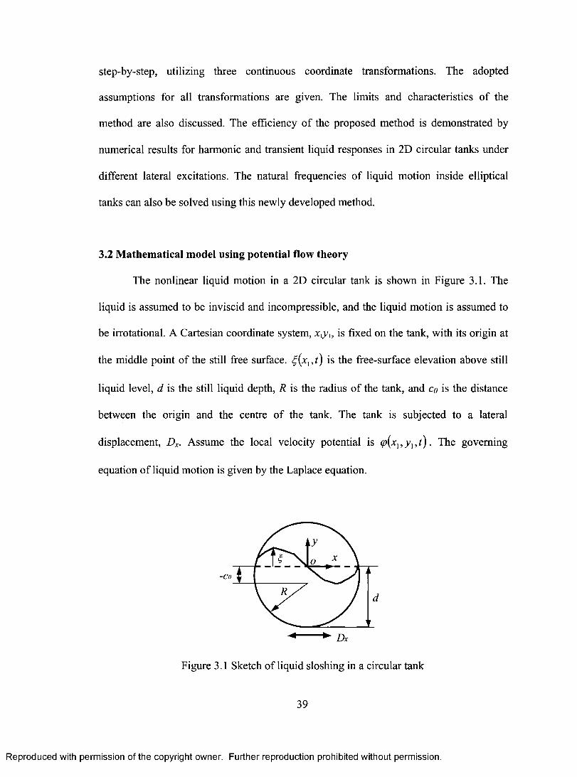
step-by-step, utilizing three continuous coordinate transformations. The adopted
assumptions for all transformations are given. The limits and characteristics of the
method are also discussed. The efficiency of the proposed method is demonstrated by
numerical results for harmonic and transient liquid responses in 2D circular tanks under
different lateral excitations. The natural frequencies of liquid motion inside elliptical
tanks can also be solved using this newly developed method.
3.2 Mathematical model using potential flow theory
The nonlinear liquid motion in a 2D circular tank is shown in Figure 3.1. The
liquid is assumed to be inviscid and incompressible, and the liquid motion is assumed to
be irrotational. A Cartesian coordinate system, xty, is fixed on the tank, with its origin at
the middle point of the still free surface. (x, ,t) is the free-surface elevation above still
liquid level, d is the still liquid depth, R is the radius of the tank, and co is the distance
between the origin and the centre of the tank. The tank is subjected to a lateral
displacement, Dx. Assume the local velocity potential is q).(xl ,yo t). The governing
equation of liquid motion is given by the Laplace equation.
Figure 3.1 Sketch of liquid sloshing in a circular tank
39
Reproduced with permission of the copyright owner. Further reproduction prohibited without permission.
step-by-step, utilizing three continuous coordinate transformations. The adopted
assumptions for all transformations are given. The limits and characteristics of the
method are also discussed. The efficiency o f the proposed method is demonstrated by
numerical results for harmonic and transient liquid responses in 2D circular tanks under
different lateral excitations. The natural frequencies of liquid motion inside elliptical
tanks can also be solved using this newly developed method.
3.2 Mathematical model using potential flow theory
The nonlinear liquid motion in a 2D circular tank is shown in Figure 3.1. The
liquid is assumed to be inviscid and incompressible, and the liquid motion is assumed to
be irrotational. A Cartesian coordinate system, x y u is fixed on the tank, with its origin at
the middle point of the still free surface. £,{xx, t) is the ffee-surface elevation above still
liquid level, d is the still liquid depth, R is the radius o f the tank, and Co is the distance
between the origin and the centre o f the tank. The tank is subjected to a lateral
displacement, Dx. Assume the local velocity potential is (p{xx, y x, t ) . The governing
equation o f liquid motion is given by the Laplace equation.
-C o
► Dx
Figure 3.1 Sketch of liquid sloshing in a circular tank
39
Reproduced with permission of the copyright owner. Further reproduction prohibited without permission.
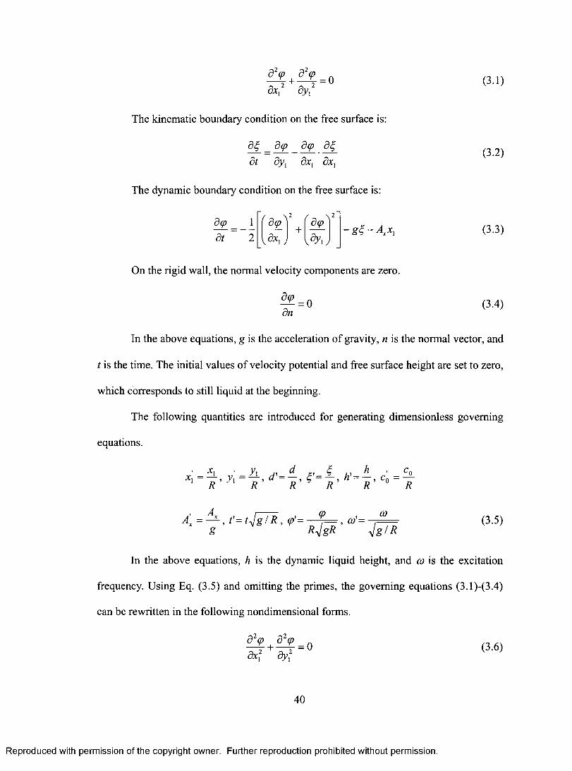
(3.1)
The kinematic boundary condition on the free surface is:
= av _aco at ay, ax, ax,
The dynamic boundary condition on the free surface is:
av i[( ac0\ 2at 2 a.x,
\
(3.2)
— g — Axxi (3.3)
On the rigid wall, the normal velocity components are zero.
aq3 —o an (3.4)
In the above equations, g is the acceleration of gravity, n is the normal vector, and
t is the time. The initial values of velocity potential and free surface height are set to zero,
which corresponds to still liquid at the beginning.
The following quantities are introduced for generating dimensionless governing
equations.
X ,
R ° R
A Ax =—' , tVg I R, (0'= r c°
g RaigR (3.5)
In the above equations, h is the dynamic liquid height, and co is the excitation
frequency. Using Eq. (3.5) and omitting the primes, the governing equations (3.1)-(3.4)
can be rewritten in the following nondimensional forms.
a2 (0 a2 co = 0
ax? ay?
40
(3.6)
Reproduced with permission of the copyright owner. Further reproduction prohibited without permission.
fix, fiy,
The kinematic boundary condition on the free surface is:
fi£ _ d(p dcp dE,dt fiy, fix, fix,
The dynamic boundary condition on the free surface is:
(3.1)
(3.2)
dcpdt
f dcp^
v& i J+
dcp
V ^ i J- g 4 - (3.3)
On the rigid wall, the normal velocity components are zero.
^ = 0dn
(3.4)
In the above equations, g is the acceleration of gravity, n is the normal vector, and
t is the time. The initial values of velocity potential and free surface height are set to zero,
which corresponds to still liquid at the beginning.
The following quantities are introduced for generating dimensionless governing
equations.
R y i -A, /,'4 .c0=%R R R R R
A'x = — , t ' = t J g / R , (p'= Z— S R jg R
, (O '' =co
(3.5)
In the above equations, h is the dynamic liquid height, and co is the excitation
frequency. Using Eq. (3.5) and omitting the primes, the governing equations (3.1)-(3.4)
can be rewritten in the following nondimensional forms.
S > f i>dxf dyx
= 0 (3.6)
40
Reproduced with permission of the copyright owner. Further reproduction prohibited without permission.
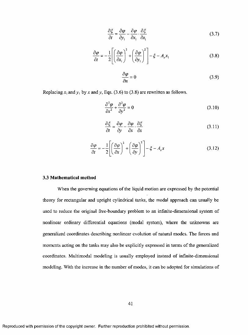
.a 4 _aco at ay, ax, ax,
ac, = _1 at 2
i aco \2 ( \2 -
ax1 .a-Y1)
ao an
— — Axx,
(3.7)
(3.8)
0 (3.9)
Replacing x, and y, by x and y, Eqs. (3.6) to (3.8) are rewritten as follows.
a2q)
+a2`)
. 0
aX2 ay 2
a = 4 _aco a at ay ax ax
4 =_ 1 at 2
(4)2 r aq) , 2
ax j + ay, _
(3.10)
(3.11)
— — Axx (3.12)
3.3 Mathematical method
When the governing equations of the liquid motion are expressed by the potential
theory for rectangular and upright cylindrical tanks, the modal approach can usually be
used to reduce the original free-boundary problem to an infinite-dimensional system of
nonlinear ordinary differential equations (modal system), where the unknowns are
generalized coordinates describing nonlinear evolution of natural modes. The forces and
moments acting on the tanks may also be explicitly expressed in terms of the generalized
coordinates. Multimodal modeling is usually employed instead of infinite-dimensional
modeling. With the increase in the number of modes, it can be adopted for simulations of
41
Reproduced with permission of the copyright owner. Further reproduction prohibited without permission.
dcpdt
c^L _dcp__dcp_ d%_ dt dy{ dx[ cbc,
dcp'2
+ fd(pTdx J
dcp0
dn
Replacing x { andy, by x andy, Eqs. (3.6) to (3.8) are rewritten as follows.
d 2tp d 2tpdx2 ay2
d£ _ dcp dcp d% dt dy dx dx
dcpdt
dcp v dx j
+dcp
j- £ - A x X
(3.7)
(3.8)
(3-9)
(3.10)
(3.11)
(3.12)
3.3 Mathematical method
When the governing equations of the liquid motion are expressed by the potential
theory for rectangular and upright cylindrical tanks, the modal approach can usually be
used to reduce the original free-boundary problem to an infinite-dimensional system of
nonlinear ordinary differential equations (modal system), where the unknowns are
generalized coordinates describing nonlinear evolution of natural modes. The forces and
moments acting on the tanks may also be explicitly expressed in terms o f the generalized
coordinates. Multimodal modeling is usually employed instead of infinite-dimensional
modeling. With the increase in the number o f modes, it can be adopted for simulations of
41
Reproduced with permission of the copyright owner. Further reproduction prohibited without permission.
realistic liquid motion. It can also be used for cases when the linear sloshing problem has
no analytical solutions, and the modes are approximated by a numeric-analytical method.
However, as pointed out by Faltinsen and Timokha (2002), it should be noted that
the modal method is a possible basis for studying sloshing with shallow, intermediate and
finite depth. It cannot describe overturning and breaking waves. The tank should have no
roof. More importantly, the tank walls in the equilibrium position must be vertical at the
mean free surface. For tanks with non-vertical walls, either inclined straight walls or
curved walls, the modes have a time-varying domain. This means the modal approach is
inapplicable even for linear sloshing problems. The actual liquid motion near the walls
cannot be described by using the modal approach and corresponding mathematical
treatments.
It should be noted that statements made by some researchers in their studies
suggesting that their methods could be used to solve sloshing problems for tanks of
arbitrary shapes could mislead readers. For example, Komatsu (1987) proposed a method
for calculating the nonlinear dynamic behaviour of liquid in tanks. The formulation used
the orthogonality of the linear mode shapes and the numerical perturbation technique.
The problem was reduced to the non-linear coupled ordinary differential equations
describing the timewise trend. The author stated that this method could deal with any
arbitrarily shaped tanks. However, because the linear solutions were pre-required in this
method, it actually cannot deal with arbitrarily shaped tanks. In fact, the method was
generally a modal method. The linear solutions were only analytically available for
rectangular and upright cylindrical containers. For tanks with non-vertical walls, it is
difficult to obtain linear solutions by either analytical or numerical method. The
42
Reproduced with permission of the copyright owner. Further reproduction prohibited without permission.
efficiency of the method had only been demonstrated by nonlinear liquid motion in
rectangular and axisymmetric upright cylindrical containers. As a matter of fact, sloshing
problem depends largely on the shapes and orientations of the tanks. It is commonly
recognized that orthogonal linear modes do not exist for tanks with curved walls. A
universal method for liquid sloshing problems cannot be pursued due to mathematical
difficulties.
Due to the unavailability of analytical solutions, a numerical method should be
used to solve the above governing equations. Obviously, the boundary conditions on the
curved walls, the nonlinearity caused by the boundary conditions on the free surface, as
well as the time-varying integration domain for the time-varying free surface are the
major difficulties in obtaining the numerical solution of sloshing problems in circular
tanks.
Existing numerical schemes for 2D sloshing problems in circular tanks usually
directly discretize the governing equations in the 2D circular area and have the following
difficulties. First, when the governing equations are described by Navier-Stokes equations
and discretized by the finite difference method, the boundary conditions on the curved
walls are quite difficult to obtain in those cells that are enclosed by curved edges and
straight edges. Computer algorithms for considering all different configurations in
interpolation for pressure and velocity components on the curved cell edges are extremely
intricate. When the governing equations are described by the potential theory and
discretized by the boundary element method, some existent algorithms for the smoothing
of the free surface position cannot be directly used in the time-varying domain caused by
the curved walls. This could be solved by changing to a polar coordinate system, which
43
Reproduced with permission of the copyright owner. Further reproduction prohibited without permission.
efficiency of the method had only been demonstrated by nonlinear liquid motion in
rectangular and axisymmetric upright cylindrical containers. As a matter o f fact, sloshing
problem depends largely on the shapes and orientations of the tanks. It is commonly
recognized that orthogonal linear modes do not exist for tanks with curved walls. A
universal method for liquid sloshing problems cannot be pursued due to mathematical
difficulties.
Due to the unavailability o f analytical solutions, a numerical method should be
used to solve the above governing equations. Obviously, the boundary conditions on the
curved walls, the nonlinearity caused by the boundary conditions on the free surface, as
well as the time-varying integration domain for the time-varying free surface are the
major difficulties in obtaining the numerical solution o f sloshing problems in circular
tanks.
Existing numerical schemes for 2D sloshing problems in circular tanks usually
directly discretize the governing equations in the 2D circular area and have the following
difficulties. First, when the governing equations are described by Navier-Stokes equations
and discretized by the finite difference method, the boundary conditions on the curved
walls are quite difficult to obtain in those cells that are enclosed by curved edges and
straight edges. Computer algorithms for considering all different configurations in
interpolation for pressure and velocity components on the curved cell edges are extremely
intricate. When the governing equations are described by the potential theory and
discretized by the boundary element method, some existent algorithms for the smoothing
of the free surface position cannot be directly used in the time-varying domain caused by
the curved walls. This could be solved by changing to a polar coordinate system, which
43
Reproduced with permission of the copyright owner. Further reproduction prohibited without permission.
in turn makes the governing equations much more complicated due to the lack of
axisymmetry in the free surface problem. Second, although the Volume of Fluid method
for free surface updating has been established and developed for many years, the
algorithms based on solving the volume fraction of the liquid in the free surface cells are
usually quite complicated for both theoretical development and programming. Third, the
above two difficulties become much more obvious when 3D sloshing in the horizontal
cylindrical tanks is to be solved.
Therefore, it is necessary to develop numerical methods that can easily deal with
the boundary conditions on the curved walls, update the free surface in the time-varying
domain without the need for complicated algorithms, as well as be extended to the 3D
problems with computational efficiency. In the following sections, a new numerical
scheme is developed for these purposes. The governing equations are rearranged by three
continuous coordinate mappings before discretization, which can avoid all of the above
difficulties in solving the sloshing problems in horizontal circular tanks.
3.3.1 First transformation
In solving the boundary conditions on curved walls, the interpolation method is
commonly employed if the governing equations are directly discretized from Eqs. (3.9) to
(3.12) in the Cartesian coordinate system. Considerable work should be carried out on the
potential expression on curved walls for different configurations. If the polar coordinates
were adopted, derivation of governing equations and implementation of calculation
would become complicated. Due to the lack of axisymmetry of the free surface problem
in partially filled tanks, the adoption of a polar coordinate system for 2D problems would
44
Reproduced with permission of the copyright owner. Further reproduction prohibited without permission.
in turn makes the governing equations much more complicated due to the lack of
axisymmetry in the free surface problem. Second, although the Volume o f Fluid method
for free surface updating has been established and developed for many years, the
algorithms based on solving the volume fraction o f the liquid in the free surface cells are
usually quite complicated for both theoretical development and programming. Third, the
above two difficulties become much more obvious when 3D sloshing in the horizontal
cylindrical tanks is to be solved.
Therefore, it is necessary to develop numerical methods that can easily deal with
the boundary conditions on the curved walls, update the free surface in the time-varying
domain without the need for complicated algorithms, as well as be extended to the 3D
problems with computational efficiency. In the following sections, a new numerical
scheme is developed for these purposes. The governing equations are rearranged by three
continuous coordinate mappings before discretization, which can avoid all o f the above
difficulties in solving the sloshing problems in horizontal circular tanks.
3.3.1 First transformation
In solving the boundary conditions on curved walls, the interpolation method is
commonly employed if the governing equations are directly discretized from Eqs. (3.9) to
(3.12) in the Cartesian coordinate system. Considerable work should be carried out on the
potential expression on curved walls for different configurations. If the polar coordinates
were adopted, derivation o f governing equations and implementation of calculation
would become complicated. Due to the lack o f axisymmetry of the free surface problem
in partially filled tanks, the adoption o f a polar coordinate system for 2D problems would
44
Reproduced with permission of the copyright owner. Further reproduction prohibited without permission.
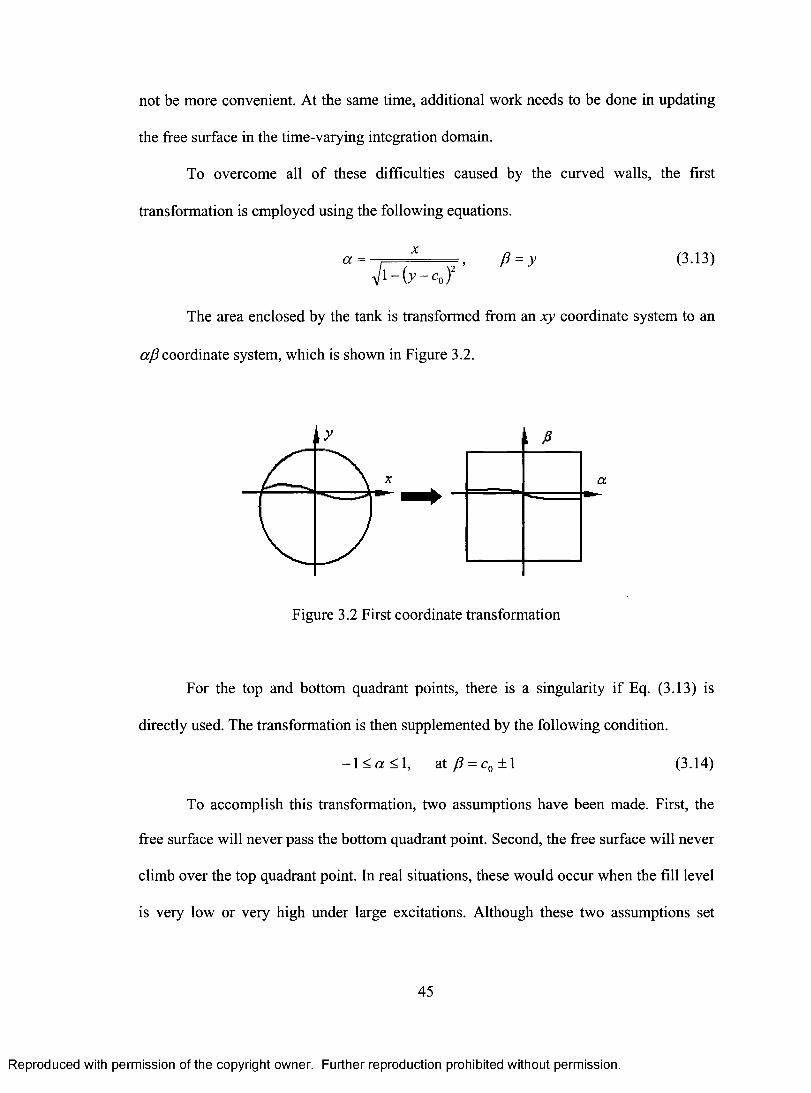
not be more convenient. At the same time, additional work needs to be done in updating
the free surface in the time-varying integration domain.
To overcome all of these difficulties caused by the curved walls, the first
transformation is employed using the following equations.
x (3.13) a = ,
Ail — (y — co )2 = y
The area enclosed by the tank is transformed from an xy coordinate system to an
a/3 coordinate system, which is shown in Figure 3.2.
A iS
a
Figure 3.2 First coordinate transformation
For the the top and bottom quadrant points, there is a singularity if Eq. (3.13) is
directly used. The transformation is then supplemented by the following condition.
—1<<—a<_1, at fi = co ± 1 (3.14)
To accomplish this transformation, two assumptions have been made. First, the
free surface will never pass the bottom quadrant point. Second, the free surface will never
climb over the top quadrant point. In real situations, these would occur when the fill level
is very low or very high under large excitations. Although these two assumptions set
45
Reproduced with permission of the copyright owner. Further reproduction prohibited without permission.
not be more convenient. At the same time, additional work needs to be done in updating
the free surface in the time-varying integration domain.
To overcome all o f these difficulties caused by the curved walls, the first
transformation is employed using the following equations.
a - P = y (3.13)V M t -C q)2
The area enclosed by the tank is transformed from an xy coordinate system to an
a f lcoordinate system, which is shown in Figure 3.2.
Figure 3.2 First coordinate transformation
For the top and bottom quadrant points, there is a singularity if Eq. (3.13) is
directly used. The transformation is then supplemented by the following condition.
- 1 < « < 1 , at /? = c0 ± 1 (3.14)
To accomplish this transformation, two assumptions have been made. First, the
free surface will never pass the bottom quadrant point. Second, the free surface will never
climb over the top quadrant point. In real situations, these would occur when the fill level
is very low or very high under large excitations. Although these two assumptions set
45
Reproduced with permission of the copyright owner. Further reproduction prohibited without permission.
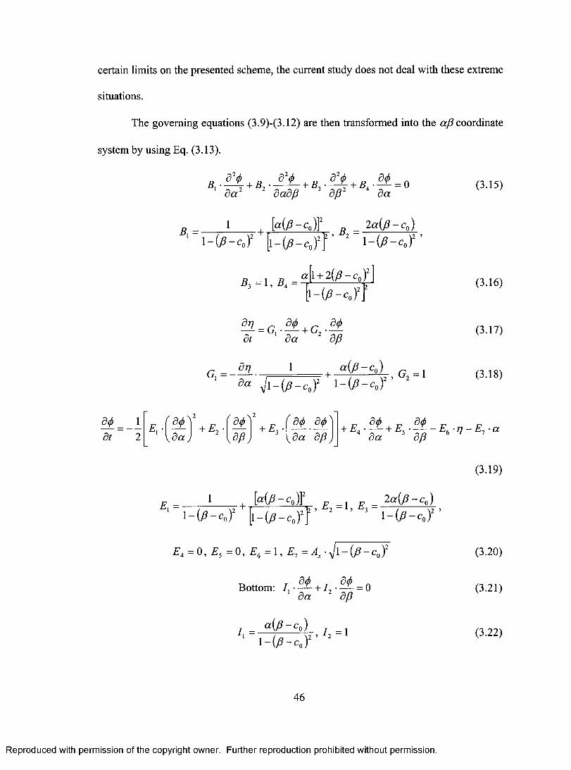
certain limits on the presented scheme, the current study does not deal with these extreme
situations.
The governing equations (3.9)-(3.12) are then transformed into the a/3 coordinate
system by using Eq. (3.13).
ao = _i[ E
at 2 1
B1
32A 02, 02A
afbB • '
1 a a 2 + B ' + B ' + B = 0
2 &tap 3 8,62 4 act
_ 1
1-(fi-00)2+ Ea(flcoA2 {i 0 — coyt , B 2 a2 1 ((flfi —C C00) )2
B3 = 1 , B4 = a 1 + 20 — c0 )2
1— (6 — co)2
871 =G•ao
at ' • —aa +G2
00
ap
a ri 1 +
46 — co ) G = I G = 1
as VI _ (fi• _ co )2 1—(p — c0)2, 2
50 2 ± E2. 50 2 ± E3 ' 80 80' + E4 . 50 ± E 50 E6
a) .8,6 ) ,aa ap , 0a 5• a/340
(3.15)
(3.16)
(3.17)
(3.18)
ri — E7 a
(3.19)
Et1 [a(B — co)12
1, E 3E 224 — co )
+
= =
, , 1 — (fi — CO ) 2 [1 — (fi — Co ) 2 f 1- (p — Co ) 2
E 4 = 0 , E 5 = 0 , E 6 = 1 , E7 = A„ •• ill — (fl — co )2 (3.20)
Bottom: 50 50 /' 12 (3.21) • a
+ -,6 =0
I1= a( 6) —c°)2 12 1 (3.22) -- , 1 — (p —Co)
46
Reproduced with permission of the copyright owner. Further reproduction prohibited without permission.
certain limits on the presented scheme, the current study does not deal with these extreme
situations.
The governing equations (3.9)-(3.12) are then transformed into the a p coordinate
system by using Eq. (3.13).
1 d a 2 2 dadp 3 dp3 a / 5 2 4 da(3.15)
Bx =[ a { p - c 0 )]2 2 a ( p - c 0)
B3 = 1, Ba =a
i P - c j f(3.16)
<h l = g a t + G mdt d a dp
dr] I | a ( p ~ c 0)
- { P - c J l - ( ^ - c 0):2 . G 2 =1
(3.17)
(3.18)
d l _ _ J_ dt ~ 2
E\ ’ + e 2 • + ^3-r dtj>_ d f
d a dp+ E4 - ^ - + E 5 ~ - E 6 ■T ] -E 7 -a
4 d a 5 d p 6 ' 7
(3.19)
£> =J , N y g -^o )]2 E =1 E _ 2 a ( p ~ c 0)
l - ( / 7 - c 0)2 l - ( / ? - c 0):
E 4 = 0 , E 5 = 0 , E 6 = 1 , E 7 = A x ^ I - ( P - c J
Bottom: /, • — + / 2 • ^ = 0d a dp
(3.20)
(3.21)
_ a { p - c 0)
2(3 .22)
46
Reproduced with permission of the copyright owner. Further reproduction prohibited without permission.
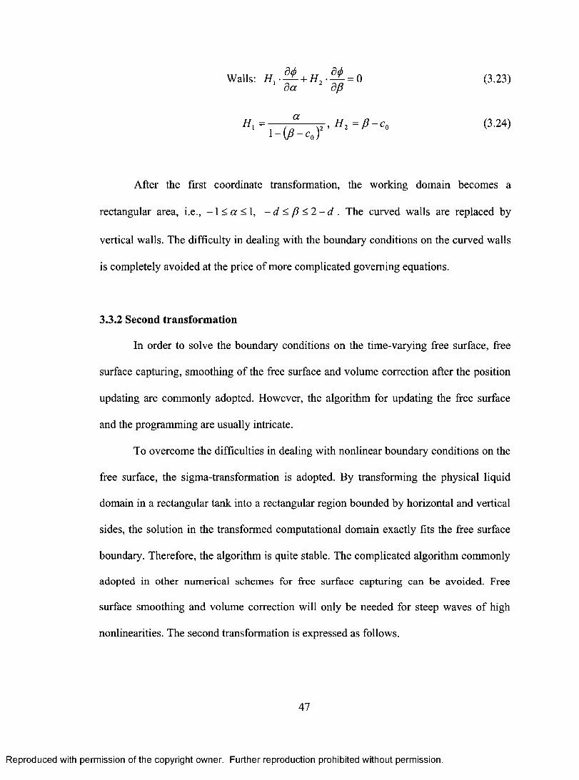
a0 _(P_a = 0 Walls: HI . T t- + H2 ap
aHI =
1—(p — co)2 , H2 =
fl
— co
(3.23)
(3.24)
After the first coordinate transformation, the working domain becomes a
rectangular area, i.e., —1 _.01 1, —,c1 /3 5 2 —d. The curved walls are replaced by
vertical walls. The difficulty in dealing with the boundary conditions on the curved walls
is completely avoided at the price of more complicated governing equations.
3.3.2 Second transformation
In order to solve the boundary conditions on the time-varying free surface, free
surface capturing, smoothing of the free surface and volume correction after the position
updating are commonly adopted. However, the algorithm for updating the free surface
and the programming are usually intricate.
To overcome the difficulties in dealing with nonlinear boundary conditions on the
free surface, the sigma-transformation is adopted. By transforming the physical liquid
domain in a rectangular tank into a rectangular region bounded by horizontal and vertical
sides, the solution in the transformed computational domain exactly fits the free surface
boundary. Therefore, the algorithm is quite stable. The complicated algorithm commonly
adopted in other numerical schemes for free surface capturing can be avoided. Free
surface smoothing and volume correction will only be needed for steep waves of high
nonlinearities. The second transformation is expressed as follows.
47
Reproduced with permission of the copyright owner. Further reproduction prohibited without permission.
After the first coordinate transformation, the working domain becomes a
rectangular area, i.e., -1 < a < 1, - d < J3 <2 - d . The curved walls are replaced by
vertical walls. The difficulty in dealing with the boundary conditions on the curved walls
is completely avoided at the price of more complicated governing equations.
3.3.2 Second transformation
In order to solve the boundary conditions on the time-varying free surface, free
surface capturing, smoothing of the free surface and volume correction after the position
updating are commonly adopted. However, the algorithm for updating the free surface
and the programming are usually intricate.
To overcome the difficulties in dealing with nonlinear boundary conditions on the
free surface, the sigma-transformation is adopted. By transforming the physical liquid
domain in a rectangular tank into a rectangular region bounded by horizontal and vertical
sides, the solution in the transformed computational domain exactly fits the free surface
boundary. Therefore, the algorithm is quite stable. The complicated algorithm commonly
adopted in other numerical schemes for free surface capturing can be avoided. Free
surface smoothing and volume correction will only be needed for steep waves o f high
nonlinearities. The second transformation is expressed as follows.
47
Reproduced with permission of the copyright owner. Further reproduction prohibited without permission.
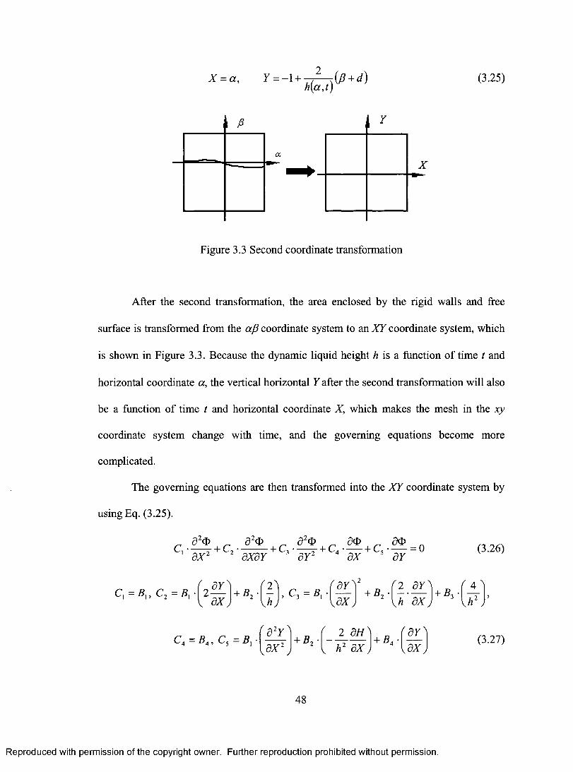
i \ X = a, Y=-1+ 2 (/3+d)
h(a ,t)
........a.m.._
46.---
a
MIIMIOP
1 Y
X
Figure 3.3 Second coordinate transformation
(3.25)
After the second transformation, the area enclosed by the rigid walls and free
surface is transformed from the afl coordinate system to an XY coordinate system, which
is shown in Figure 3.3. Because the dynamic liquid height h is a function of time t and
horizontal coordinate a, the vertical horizontal Y after the second transformation will also
be a function of time t and horizontal coordinate X, which makes the mesh in the xy
coordinate system change with time, and the governing equations become more
complicated.
The governing equations are then transformed into the XY coordinate system by
using Eq. (3.25).
2 0 2 20 c
a +c +C., +c •—+c —=o
' ax2 2 a
aXaY a aY2 4
ao ax 5
ao ay
(3.26)
ay 2 ay)2 (
h 2 ay
ax 1 - - ) B
1 1i
C, =B,, C2 = 131 . (2 —) + B2 • ( h ) , C3 = 13, (ax)
+B2 • — 1ax 172)'
( 2 all) (all a2Y)+B2 (— h2
—ax j+ B4 CaTc ) ,ax2
48
(3.27)
Reproduced with permission of the copyright owner. Further reproduction prohibited without permission.
X = a, Y = - 1 +h{a,t)
( p + d ) (3.25)
Figure 3.3 Second coordinate transformation
After the second transformation, the area enclosed by the rigid walls and free
surface is transformed from the af3 coordinate system to an X Y coordinate system, which
is shown in Figure 3.3. Because the dynamic liquid height h is a function o f time t and
horizontal coordinate a, the vertical horizontal Y after the second transformation will also
be a function of time t and horizontal coordinate X, which makes the mesh in the xy
coordinate system change with time, and the governing equations become more
complicated.
The governing equations are then transformed into the X Y coordinate system by
using Eq. (3.25).
C, d 20 d 2o dO1 d x 2 2
+ C->----------1- C , ------T- + C , -------b C , ----- — 0dXdY 3 BY3 4 ax BY
(3.26)
C\ =B . , C2 = B ,BY_8 X
+ B-, , C3 — B\\ n j
BY y B X ,
+ *r 2 B Y "'
h BX+ 5 3 -
J \ n j
C4 = B , , C5 = B, f d 2 y ) + B 2 ■( 2 BH']
+ B. ■------------[d X 2J
2 L h 2 BX) 4 lax) (3.27)
48
Reproduced with permission of the copyright owner. Further reproduction prohibited without permission.
51-1 ac =Ki . ao +lcat ax 2 aY
Ki =GI , K2 = G, • ( ay` ,ax ,
ac _ 1 [ ji r ao )2 +.12 r 2+.13.rao at at 2 aX
`aY, ax aY)
ao ao+ J 4 •—+ J 5 • ay J 6 •H — J 7 • AT
ax
, ay,2 J 1 = El , J 2 = El +E2 • (-4-- + E • —
\ aX j h 2 , 3
J 3 = Ei •(2 ay` ax
2 + E3 *(77), J 4 = 0, J 5 = —
Bottom:
( ay 2`
ax h,
ay at '
J6
= E6 '
J7
= E7
1. r alc. T aCD n1 • — + L 2 - = V ax aY
ay 2L1 =11 , L2 = 1.1 *( ax )+12 •
hj
N1•P-41)
+N2 -a4:1)
= 0 Walls: ax aY
NI = 11,, N2 =111( ay`,ax ,
+H2 •(-2 )
(3.28)
(3.29)
(3.30)
(3.31)
(3.32)
(3.33)
(3.34)
(3.35)
The application of the second transformation introduces the following
relationships, taking into account that the vertical coordinate is a function of time and the
horizontal coordinate.
ay ax -
Y+1 (au) a2y 2(Y+1) ( afi`2 Y+1 7 a2H` h ax )' ax2 h 2 \ ax , h ax2 J
ay Y +1 (al at h at
49
(3.36)
Reproduced with permission of the copyright owner. Further reproduction prohibited without permission.
dH „ 5 0 ^ 5 0 — Ki •------h Kj * —dt dX 2 dY
K, = G,, K 2 = G{ ■ + G2 •f - 1l a * ; 4 yk y
5 0dt
^ 5 0 ^ 25X
+ J^ 5 0 ^ 2
5 0
v 5 7 y+ ./-)
5 0 5 05W 57
5 0+ J 4 + J 5 J 6 - H - J 7 - X
dx
J \ = E \ , J 2 = E \ ■
dY
f
y d X j
f A \+ E 2 ■
k« 2j+ e 3 -
dY 2d x ' H
J 3 = E r( ? dY_) { dXj
r?L \h j
Bottom:
57/ = 0 T I = F I - F,i7 4 w , */ 5 — ^ ^ 6 6 1 J 1 ~dt
50 50L, b T-, ■ — — 0
1 5J7 2 57
L\ — I \ , L 2 — I x -r 57 A
v5Zy+ / 2 •
'2 ^
U y
Walls:5 0 5 0
N , + N 2 = 01 dx 2 dY
N\ - H x, N 2 - H { ■ + H 2 ■r 2 s
[ d X j 2 ^ y
(3.28)
(3.29)
(3.30)
(3.31)
(3.32)
(3.33)
(3.34)
(3.35)
The application of the second transformation introduces the following
relationships, taking into account that the vertical coordinate is a function o f time and the
horizontal coordinate.
dY 7 + 1 ( d H ^ 527 _ 2 (7 + i; ( d H \ 2 7 + 1 ( d 2H \dX h la*J ’ d X 2 h2 \ dX j h [ d X 2 J
57dt
7 + 1 rd H '
s. dt V(3.36)
49
Reproduced with permission of the copyright owner. Further reproduction prohibited without permission.
The second transformation is exactly the so-called sigma-transformation, which
was first proposed by Phillips (1957) for numerical forecasting. It has recently been
applied in the research of hydrodynamics and sloshing in combination with different
numerical methods. For example, it has been used in research on pressures on dams by
Navier-Stokes equations and the finite difference method (Chen, 1994), 2-D sloshing in
rectangular containers by the potential theory and the pseudospectral method (Chern et al,
1999), 3-D standing and impulse waves in an upright cylindrical container with a central
cylindrical inclusion by the potential theory and the spectral method (Chern et al, 2001),
2-D sloshing in rectangular containers by the potential theory and the finite element
method (Turnbull et al, 2003), and 2-D sloshing in rectangular containers by the potential
theory and the finite difference method (Frandsen, 2003). However, an application of
this approach in analyzing the liquid motion in a horizontal cylindrical tank is not found
in the current literature.
To perform the second transformation, another assumption is needed. Since the
free surface height is expressed as a single value function of the horizontal coordinate and
stretched in the direction of the vertical coordinate, overturning waves and breaking
waves cannot be described. Therefore, it is assumed that overturning waves and breaking
waves are not involved in the current study. This again sets certain limits on the proposed
method. This extreme situation is not considered in this research. It should also be noted
that the application of the second transformation, which is one type of the boundary fitted
method, makes it unsuitable for large excitations. It is well known that the simple
algebraic mappings are not robust when the free surface is quite steep. Therefore, high
nonlinearity such as a wave with large steepness is not considered in this study. The
50
Reproduced with permission of the copyright owner. Further reproduction prohibited without permission.
The second transformation is exactly the so-called sigma-transformation, which
was first proposed by Phillips (1957) for numerical forecasting. It has recently been
applied in the research o f hydrodynamics and sloshing in combination with different
numerical methods. For example, it has been used in research on pressures on dams by
Navier-Stokes equations and the finite difference method (Chen, 1994), 2-D sloshing in
rectangular containers by the potential theory and the pseudospectral method (Chem et al,
1999), 3-D standing and impulse waves in an upright cylindrical container with a central
cylindrical inclusion by the potential theory and the spectral method (Chem et al, 2001),
2-D sloshing in rectangular containers by the potential theory and the finite element
method (Turnbull et al, 2003), and 2-D sloshing in rectangular containers by the potential
theory and the finite difference method (Frandsen, 2003). However, an application of
this approach in analyzing the liquid motion in a horizontal cylindrical tank is not found
in the current literature.
To perform the second transformation, another assumption is needed. Since the
free surface height is expressed as a single value function of the horizontal coordinate and
stretched in the direction of the vertical coordinate, overturning waves and breaking
waves cannot be described. Therefore, it is assumed that overturning waves and breaking
waves are not involved in the current study. This again sets certain limits on the proposed
method. This extreme situation is not considered in this research. It should also be noted
that the application o f the second transformation, which is one type o f the boundary fitted
method, makes it unsuitable for large excitations. It is well known that the simple
algebraic mappings are not robust when the free surface is quite steep. Therefore, high
nonlinearity such as a wave with large steepness is not considered in this study. The
50
Reproduced with permission of the copyright owner. Further reproduction prohibited without permission.
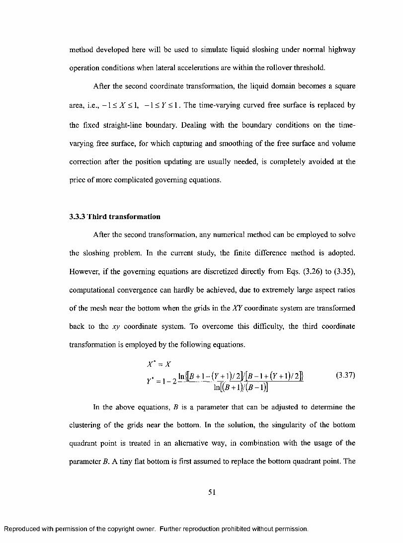
method developed here will be used to simulate liquid sloshing under normal highway
operation conditions when lateral accelerations are within the rollover threshold.
After the second coordinate transformation, the liquid domain becomes a square
area, i.e., —1 X Y 1. The time-varying curved free surface is replaced by
the fixed straight-line boundary. Dealing with the boundary conditions on the time-
varying free surface, for which capturing and smoothing of the free surface and volume
correction after the position updating are usually needed, is completely avoided at the
price of more complicated governing equations.
3.3.3 Third transformation
After the second transformation, any numerical method can be employed to solve
the sloshing problem. In the current study, the finite difference method is adopted.
However, if the governing equations are discretized directly from Eqs. (3.26) to (3.35),
computational convergence can hardly be achieved, due to extremely large aspect ratios
of the mesh near the bottom when the grids in the XY coordinate system are transformed
back to the xy coordinate system. To overcome this difficulty, the third coordinate
transformation is employed by the following equations.
X* = X
Y =1 214B +1— (Y +1)/ 210 —1+ (Y + 1)/ 211
ln[(B +1)/(B —1)]
(3.37)
In the above equations, B is a parameter that can be adjusted to determine the
clustering of the grids near the bottom. In the solution, the singularity of the bottom
quadrant point is treated in an alternative way, in combination with the usage of the
parameter B. A tiny flat bottom is first assumed to replace the bottom quadrant point. The
51
Reproduced with permission of the copyright owner. Further reproduction prohibited without permission.
method developed here will be used to simulate liquid sloshing under normal highway
operation conditions when lateral accelerations are within the rollover threshold.
After the second coordinate transformation, the liquid domain becomes a square
area, i.e., - \< X < 1, -1 < F < 1. The time-varying curved free surface is replaced by
the fixed straight-line boundary. Dealing with the boundary conditions on the time-
varying free surface, for which capturing and smoothing of the free surface and volume
correction after the position updating are usually needed, is completely avoided at the
price o f more complicated governing equations.
3.3.3 Third transformation
After the second transformation, any numerical method can be employed to solve
the sloshing problem. In the current study, the finite difference method is adopted.
However, if the governing equations are discretized directly from Eqs. (3.26) to (3.35),
computational convergence can hardly be achieved, due to extremely large aspect ratios
o f the mesh near the bottom when the grids in the X Y coordinate system are transformed
back to the xy coordinate system. To overcome this difficulty, the third coordinate
transformation is employed by the following equations.
X* - X... . , ln{|£ +1 - (y + 1)/ 2l/[fl -1 + (y + 1)/ 2P (3.37)
ln[(fi + l ) / ( 5 - l ) ]
In the above equations, B is a parameter that can be adjusted to determine the
clustering o f the grids near the bottom. In the solution, the singularity o f the bottom
quadrant point is treated in an alternative way, in combination with the usage o f the
parameter B. A tiny flat bottom is first assumed to replace the bottom quadrant point. The
51
Reproduced with permission of the copyright owner. Further reproduction prohibited without permission.
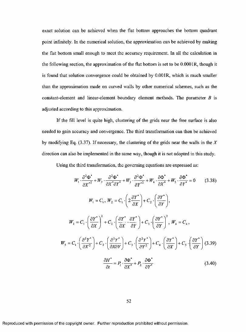
exact solution can be achieved when the flat bottom approaches the bottom quadrant
point infinitely. In the numerical solution, the approximation can be achieved by making
the flat bottom small enough to meet the accuracy requirement. In all the calculation in
the following section, the approximation of the flat bottom is set to be 0.0001R, though it
is found that solution convergence could be obtained by 0.001R, which is much smaller
than the approximation made on curved walls by other numerical schemes, such as the
constant-element and linear-element boundary element methods. The parameter B is
adjusted according to this approximation.
If the fill level is quite high, clustering of the grids near the free surface is also
needed to gain accuracy and convergence. The third transformation can then be achieved
by modifying Eq. (3.37). If necessary, the clustering of the grids near the walls in the X
direction can also be implemented in the same way, though it is not adopted in this study.
Using the third transformation, the governing equations are expressed as:
a2 * a20*
* 52 . ao* a W, +W2 +Tf73 0* +P V4 * +W5 (I)* = 0 (3.38)
ax 2 ax*ay ay 2 ax ay
W3 = C 1 •
W 5 = C 1 •
WI = C 1 , W 2 = CI • (2 + C 2
i a Y *
a Y /
,- ,2 ay* 1 'ay* ay* -F C3 ' ay*\ 2+c2 , W4 = C4 , ax, ax ay \ ay , i I
I a2 Y* \
, ax 2 1 + C2
a 2 y*
axaY i + C 3
(a2y*) (ay* \ laY*)
ay2 + C 4 ax , ± C5 , ay (3.39)
ax* ao* ao*at
= PI ax*
+P2 aY *
52
(3.40)
Reproduced with permission of the copyright owner. Further reproduction prohibited without permission.
exact solution can be achieved when the flat bottom approaches the bottom quadrant
point infinitely. In the numerical solution, the approximation can be achieved by making
the flat bottom small enough to meet the accuracy requirement. In all the calculation in
the following section, the approximation of the flat bottom is set to be 0.0001R, though it
is found that solution convergence could be obtained by 0.001 R, which is much smaller
than the approximation made on curved walls by other numerical schemes, such as the
constant-element and linear-element boundary element methods. The parameter B is
adjusted according to this approximation.
If the fill level is quite high, clustering o f the grids near the free surface is also
needed to gain accuracy and convergence. The third transformation can then be achieved
by modifying Eq. (3.37). If necessary, the clustering o f the grids near the walls in the X
direction can also be implemented in the same way, though it is not adopted in this study.
Using the third transformation, the governing equations are expressed as:
d20* d20* d20 * dO* dO*Wl - ^ r + W2 - . . +W3 - ^ t + W4 - ^ t + W5 - ^ - v = 0 (3.38)
1 ax dX dY dY dX 5 dY
wx= c {, w 2 = c x8 X\
+ C,/ v d F y
W3 = C rr dY*vv d X y
+ C2 •r dY* d Y*A
dX dY+ C3 -
r d Y * ^ 2
v dY jw = c, rr * — v 4 ,
w5 = c , . f a 2 r l + c , •f d 2Y* "1+ C 3 -f d 2Y*) + < v r dY* "1+ c5 ■( dY* ^
U x 2 J [dXdF J d Y 2 \ U1 J U f J (3.39)
dH* n dO* n dO*■ = P,- — r + P, •-
dt dX dY(3.40)
52
Reproduced with permission of the copyright owner. Further reproduction prohibited without permission.
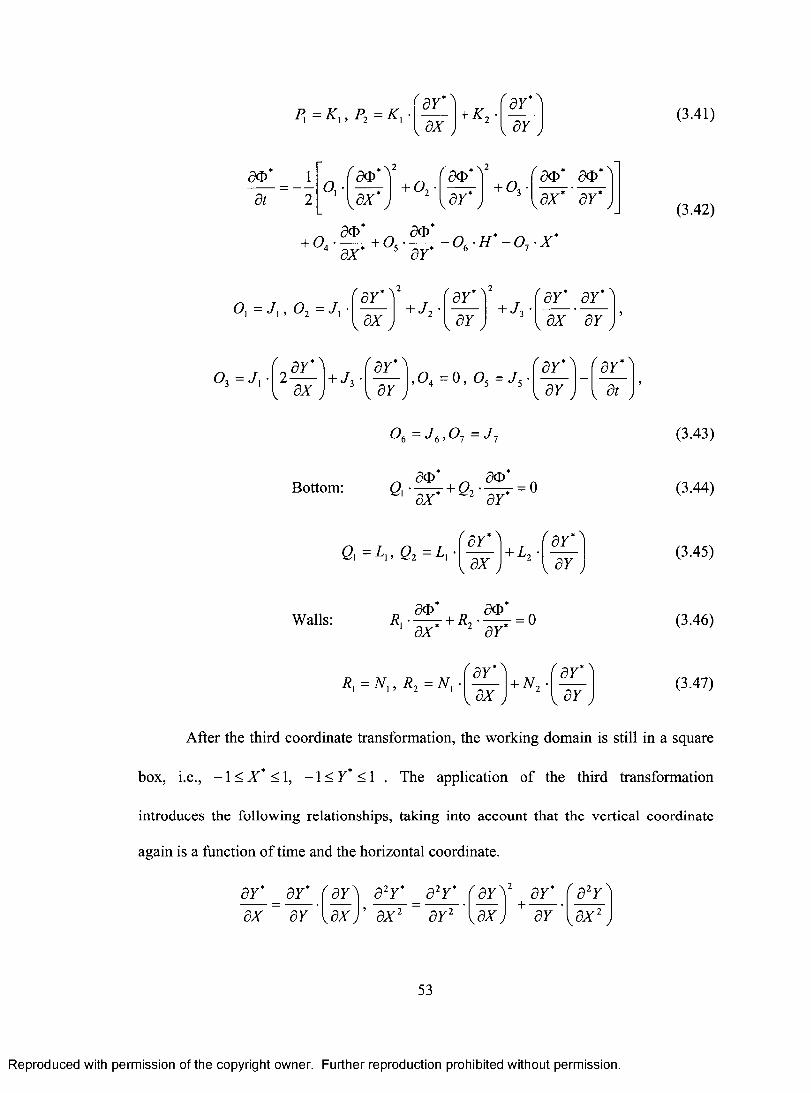
p = KI , P2 = K1gay .
ax + K2 •aY'
• ay
at 2 ax* - a Y * - ax* a Y * = 0, i + 0, i + 0,
ate ate` 'ate..•\2, * N2 racD* 1 acD
acD* acD* +o • +05 • OH• * —0 -X 7 4 ax* ay* 6
= , 02 = J 1 •
✓ * -\ 2 ay ay ay* ay" + * +J3 • ax 1 ay, ax ay,
• ay* ay' ay* ay* 0 3 =J, • 2 / +J3 ' \ , 04 = 0 , 05 =J5 '\• ax ay ay at
Bottom:
Q1 = , Q2 =L, •
06 = J6 , 0 7 =
acD* a Ql * +Q2
ate`= 0ax ay
ay* ax
+ L2
Walls: RI • ac= +R2 aCD
= 0 ax* ay*
R,= N,, R2 = NI • ( ay* \
ax + N2
ay* ay
ay* ay
(3.41)
(3.42)
(3.43)
(3.44)
(3.45)
(3.46)
(3.47)
After the third coordinate transformation, the working domain is still in a square
box, i.e., —1 x* 51, —1 Y* 1 . The application of the third transformation
introduces the following relationships, taking into account that the vertical coordinate
again is a function of time and the horizontal coordinate.
ay* ay* ray a2Y* a2Y* rayi ay* ( a2y` ax ay ,ax) ' axe ay2 aY ax2
53
Reproduced with permission of the copyright owner. Further reproduction prohibited without permission.
px= k x, p2 = k f a y * l + k 2 ■f 57* A[ s * J L I 57 J
50Bt
1 O, ■
f 50* ^2
f2
( 50* 50* 1+ * + On '2 U * ' J L 5 7 ' J [dX' 5 7 'J
50* 50*+ 0 A- ^ T + 0 5 - ^ v - 0 6 -H - 0 7 X
4 8X 5 57 6 7
0, = Jx, 0 2 = J, f BY*2
f2
r 57* 57*+ J 2 ■ + A ■[ s x ) 1 5 7 J ^5W 57 J
0 3 = J X f BY*) f 5 7 *1+ Jn 'I M jJ
CD
,o. = o , a = a
° 6 = J 6 ’ ° 7 = J 1
r b y*^v 5 7 y
Bottom:50
0 , - ^ + 02 ' 5W 2
5057*
= 0
0i - A ’ 02 — A + L7 •[ax) 2 I 57 J
Walls: A - ^ + ^ - ~ = 05A
/2 ,=W1, /22 = W 1-
57
r 57*^ + n 2 ■f 5 7 *1L [ 5 7 J
(3.41)
(3.42)
(3.43)
(3.44)
(3.45)
(3.46)
(3.47)
After the third coordinate transformation, the working domain is still in a square
box, i.e., - 1 < X * < 1 , — 1 < 7* < 1 . The application of the third transformation
introduces the following relationships, taking into account that the vertical coordinate
again is a function o f time and the horizontal coordinate.
57 57dX 57
^ 5 7 ^ \dX ;
5 7 5 7BX BY2
r BY^\d X j
+ -5757
f 5 2f A
v5.W y
53
Reproduced with permission of the copyright owner. Further reproduction prohibited without permission.
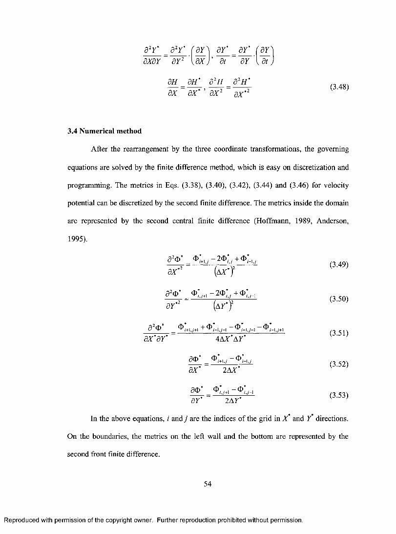
a2ye = a 2y* (ay) ay* ay ail axay ay2 ax at ay* ( at )
ax _51-1* 82H _32H* ax axe' ' ax2 ax*2
(3.48)
3.4 Numerical method
After the rearrangement by the three coordinate transformations, the governing
equations are solved by the finite difference method, which is easy on discretization and
programming. The metrics in Eqs. (3.38), (3.40), (3.42), (3.44) and (3.46) for velocity
potential can be discretized by the second finite difference. The metrics inside the domain
are represented by the second central finite difference (Hoffmann, 1989, Anderson,
1995).
ago' 4)* —24)* + 41:0*
ax' = (Ax*)2
,320* — 20;4 + (I),* (AY* )2 ay *2
a2c,* ax*ay*
i+i,J+1+ 4AX*AY*
ac* _ 0,.+1,; (13,_1, ax* 2AX*
_ OY* 2AY*
(3.49)
(3.50)
(3.51)
(3.52)
(3.53)
In the above equations, i and j are the indices of the grid in x* and y* directions.
On the boundaries, the metrics on the left wall and the bottom are represented by the
second front finite difference.
54
Reproduced with permission of the copyright owner. Further reproduction prohibited without permission.
a 2r* a 2r* ^ a r ^ ar*
#
1 r a r^ ja x a r
i
CD [ a x j ’ 8 t a r U J
8 H 8 H * 8 2H 8 2H8x 8x’ ax2 a x
*2 (3.48)
3.4 Numerical method
After the rearrangement by the three coordinate transformations, the governing
equations are solved by the finite difference method, which is easy on discretization and
programming. The metrics in Eqs. (3.38), (3.40), (3.42), (3.44) and (3.46) for velocity
potential can be discretized by the second finite difference. The metrics inside the domain
are represented by the second central finite difference (Hoffmann, 1989, Anderson,
1995).
a2o* _o*+1J - 2o ’ .+o;_1>y.ax’2 (ax*)2
a2o* o ’,+1 - 2 0 ’ . + o ’y._, ar’2 (at*)2
a 2o* ®;-u+.ax 8 Y 4AX AT
ao’ < i j - K u ax’ 2 AX*
ao’ _ o*y+l - o ’
(3.49)
(3.50)
(3.51)
(3.52)
(3.53)ar 2A y
In the above equations, i and j are the indices of the grid in X* and T* directions.
On the boundaries, the metrics on the left wall and the bottom are represented by the
second front finite difference.
54
Reproduced with permission of the copyright owner. Further reproduction prohibited without permission.
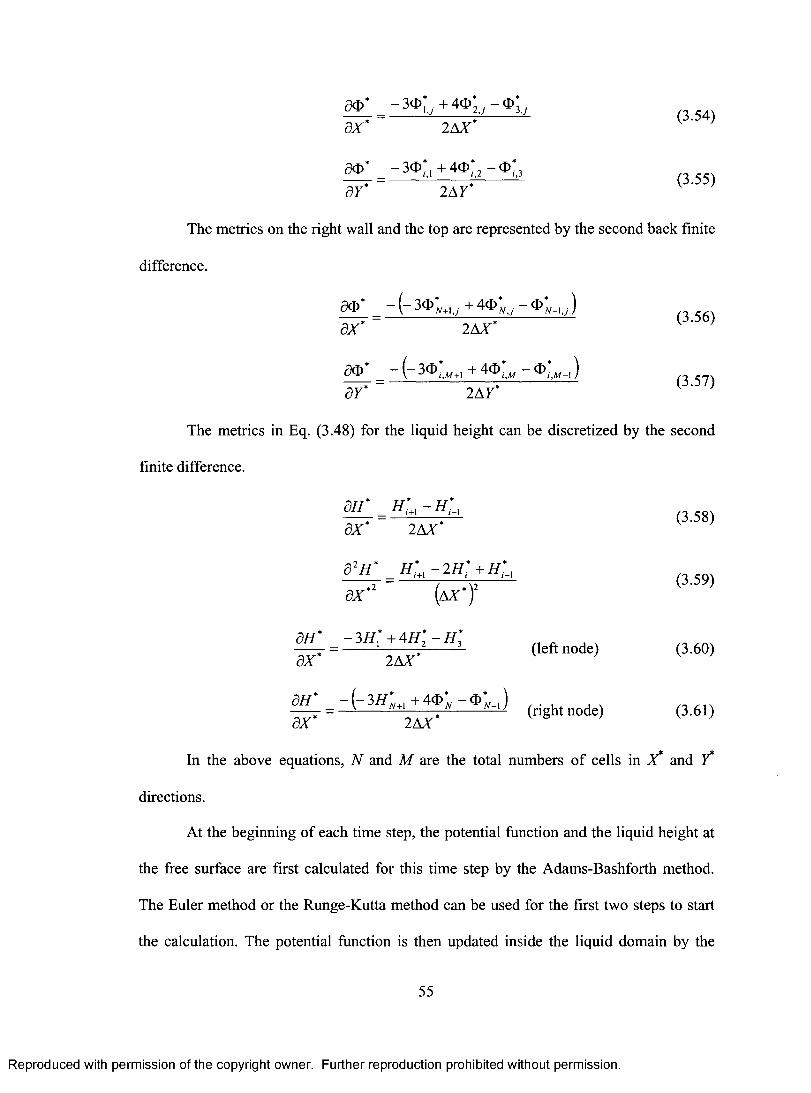
al)* — 34:13*,/ + 4(I)* 1ax* 2AX*
ao* 4o*;2 - (ID*13
ay* - 2AY*
(3.54)
(3.55)
The metrics on the right wall and the top are represented by the second back finite
difference.
ao* -(-30N+.,; + 40,1 ax* - 2AX*
ate' = — 3€1) +1 + m )
ay* 2AY*
(3.56)
(3.57)
The metrics in Eq. (3.48) for the liquid height can be discretized by the second
finite difference.
au* H* — H*= i+i ax* 2AX*
a2 H* H:+1 — 2H: + 1/:_1
ax * 2
au* -3H; + 4H; — H;
ax* 2AX* (left node)
* * +,ail* -(-31- i N + 4oN - (1)*N_ I ) - (right node) ax* 2AX*
(3.58)
(3.59)
(3.60)
(3.61)
In the above equations, N and M are the total numbers of cells in A" and Y*
directions.
At the beginning of each time step, the potential function and the liquid height at
the free surface are first calculated for this time step by the Adams-Bashforth method.
The Euler method or the Runge-Kutta method can be used for the first two steps to start
the calculation. The potential function is then updated inside the liquid domain by the
55
Reproduced with permission of the copyright owner. Further reproduction prohibited without permission.
a$* - 3 o ; .+ 4 o ; . - o 3/.d X * 2 AX*
ao* - 3 0 * , +4®*2 - 0 * 3
(3.54)
(3.55)8Y 2A Y
The metrics on the right wall and the top are represented by the second back finite
difference.
a®* -(-3®,., j +«>».,-® »-Jax* 2 AX*
ao* - ( - 3 0 * M+1+ 4 0 ^ - 0 * ^ , )
(3.56)
(3.57)a r 2A7
The metrics in Eq. (3.48) for the liquid height can be discretized by the second
finite difference.
dH* _ H*m
ax* 2 AX*
a2//* h m - i h , + //,„ax*2 (a x ’)2
dH _ - 3 H x + 4H 2 ~ h ; ~d)C~ 2 AX*
m ' - ( - 3 # ; +1+ 4 q ; - q ; . , ) ax* 2 AX*
(3.58)
(3.59)
(left node) (3.60)
(right node) (3.61)
In the above equations, N and M are the total numbers o f cells in X and Y
directions.
At the beginning of each time step, the potential function and the liquid height at
the free surface are first calculated for this time step by the Adams-Bashforth method.
The Euler method or the Runge-Kutta method can be used for the first two steps to start
the calculation. The potential function is then updated inside the liquid domain by the
55
Reproduced with permission of the copyright owner. Further reproduction prohibited without permission.
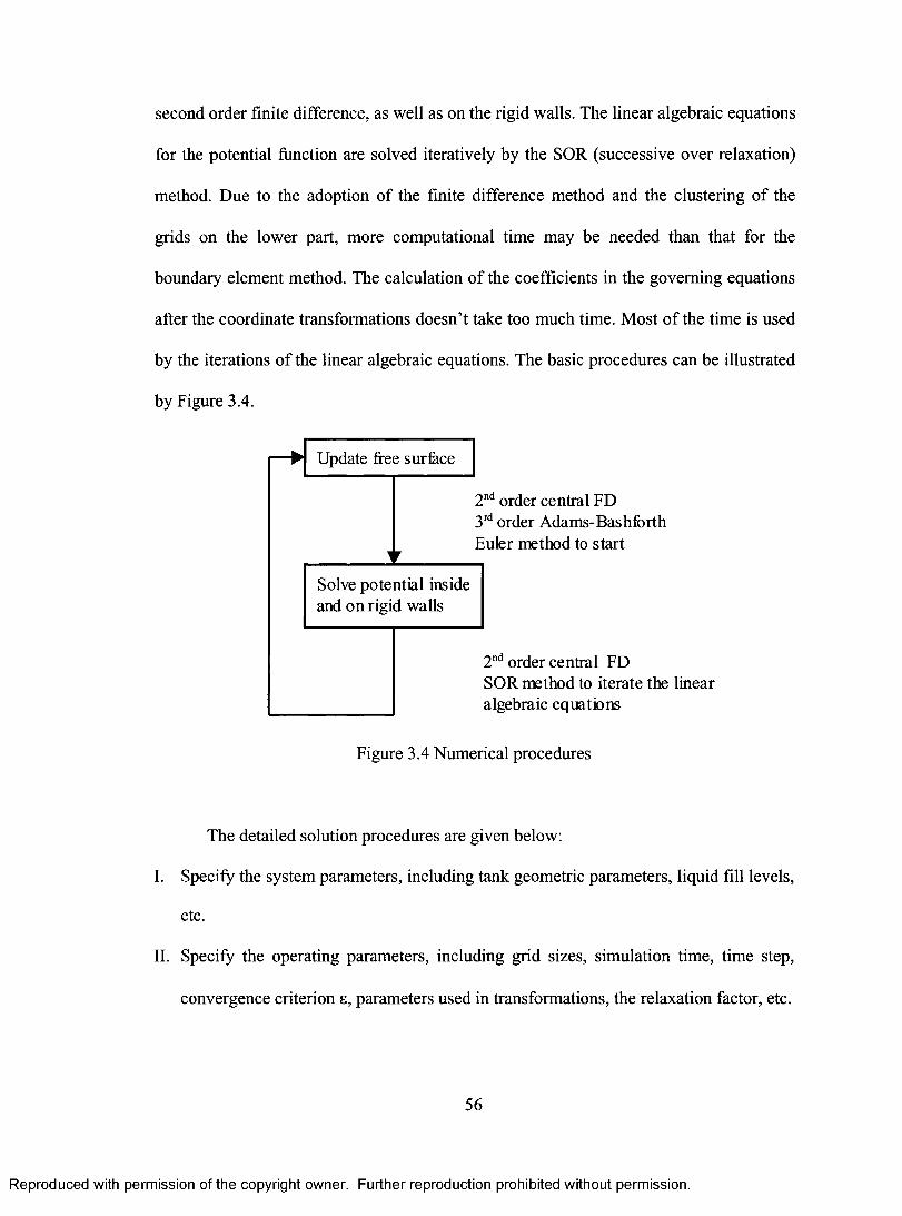
second order finite difference, as well as on the rigid walls. The linear algebraic equations
for the potential function are solved iteratively by the SOR (successive over relaxation)
method. Due to the adoption of the finite difference method and the clustering of the
grids on the lower part, more computational time may be needed than that for the
boundary element method. The calculation of the coefficients in the governing equations
after the coordinate transformations doesn't take too much time. Most of the time is used
by the iterations of the linear algebraic equations. The basic procedures can be illustrated
by Figure 3.4.
Update free surface
2❑d order central FD 3rd order Adams- Bas hfo rth Euler method to start
Solve potential inside and on rigid walls
2nd order central FD SOR method to iterate the linear algebraic equations
Figure 3.4 Numerical procedures
The detailed solution procedures are given below:
I. Specify the system parameters, including tank geometric parameters, liquid fill levels,
etc.
II. Specify the operating parameters, including grid sizes, simulation time, time step,
convergence criterion c, parameters used in transformations, the relaxation factor, etc.
56
Reproduced with permission of the copyright owner. Further reproduction prohibited without permission.
second order finite difference, as well as on the rigid walls. The linear algebraic equations
for the potential function are solved iteratively by the SOR (successive over relaxation)
method. Due to the adoption of the finite difference method and the clustering of the
grids on the lower part, more computational time may be needed than that for the
boundary element method. The calculation o f the coefficients in the governing equations
after the coordinate transformations doesn’t take too much time. Most o f the time is used
by the iterations o f the linear algebraic equations. The basic procedures can be illustrated
by Figure 3.4.
2nd order central FD 3 rd order Adams-Bashforth Euler method to start
2nd order central FDSOR method to iterate the linearalgebraic equations
Update free surface
Solve potential inside and on rigid walls
Figure 3.4 Numerical procedures
The detailed solution procedures are given below:
I. Specify the system parameters, including tank geometric parameters, liquid fill levels,
etc.
II. Specify the operating parameters, including grid sizes, simulation time, time step,
convergence criterion s, parameters used in transformations, the relaxation factor, etc.
56
Reproduced with permission of the copyright owner. Further reproduction prohibited without permission.
III. Specify the excitations for the specific operation: amplitude and frequency for sway,
final steady acceleration and input time for turning, the excitation function for lane
change and double lane change, etc.
IV. Specify initial values for liquid height and velocity potential.
V. Calculate Y*, Y, ay*
and a2y* , X*, X, a, x,
ax* and a' x* aY ay' ax ax2 •
VI. Calculate the initial pressures on the walls if the forces and moments are needed.
VII. Start the calculation in the time domain: if Time < TotalTime
i. Calculate the liquid forces (if needed):
1. Calculate liquid forces in x and y direction for the last time step based on the
liquid pressure distributions.
ii. Update the free surface:
ao* ao* art ari 2. Calculate * , * , * and — on the free surface.
ax aY ax ax
3. For each node on the free surface, calculate
ay ay ay* aY* (1) , — according to Eq. (3.36) and — according to Eq.(4.38);
ax at ax ' at
(2) the coefficients in Eqs. (3.20), (3.31), (3.43), (3.18), (3.29) and (3.41).
4. Calculate ate
and ail*
according to Eqs. (3.42) and (3.40). at at
5. Update the velocity potential and the liquid height on the free surface by:
(1) the Euler method for the first two time steps;
(2) the Adams-Bashforth method after the first two time steps.
6. (Only necessary for situations where convergence is difficult) Smooth the
velocity potential and liquid height on the free surface.
57
Reproduced with permission of the copyright owner. Further reproduction prohibited without permission.
III. Specify the excitations for the specific operation: amplitude and frequency for sway,
final steady acceleration and input time for turning, the excitation function for lane
change and double lane change, etc.
IV. Specify initial values for liquid height and velocity potential.
„ ^ __ ar* J a2r* ^ v ex* J d2x 'V. Calculate Y , Y , a n d — ,X ,X. a , x , a n d —.
ar a r2 d x d x 2
VI. Calculate the initial pressures on the walls if the forces and moments are needed.
VII. Start the calculation in the time domain: if Time < TotalTime
i. Calculate the liquid forces (if needed):
1. Calculate liquid forces in x and y direction for the last time step based on the
liquid pressure distributions.
ii. Update the free surface:
2. Calculate , ^ r and on the free surface.d x ar e x s x
3. For each node on the free surface, calculate
ar ar ar* ar*(1)— , — according to Eq. (3.36) a n d , according to Eq.(4.38);
dX dt dX dt
(2) the coefficients in Eqs. (3.20), (3.31), (3.43), (3.18), (3.29) and (3.41).
ao* dH*4. C alculate a n d according to Eqs. (3.42) and (3.40).
dt dt
5. Update the velocity potential and the liquid height on the free surface by:
(1) the Euler method for the first two time steps;
(2) the Adams-Bashforth method after the first two time steps.
6. (Only necessary for situations where convergence is difficult) Smooth the
velocity potential and liquid height on the free surface.
57
Reproduced with permission of the copyright owner. Further reproduction prohibited without permission.
iii. Solve potential inside and on the rigid walls:
aH* 52H* aft ail 7. Calculate and
ax* ' ax*2 ' ax ax
8. Calculate the coefficients
(1) in (3.22), (3.33), (3.45) for the bottom;
(2) in (3.16), (3.27), (3.39) for the inside;
(3) in (3.23), (3.35), (3.47) for the bottom for the left and right wall.
9. Solve the linear algebraic equations for the velocity potential by SOR.
If Convergence < c and Iteration number < Maximum iteration number
Stop the iteration and go to step 10;
If Convergence > c and Iteration number < Maximum iteration number
Continue the iteration;
If Convergence > c and Iteration number > Maximum iteration number
Stop and report the problem even if the convergence still could be
achieved by increasing the maximum iteration number.
10. Calculate the pressure distribution (if forces and moments are needed) on the
walls for the next time step.
11. Repeat steps 1-10 until the end of the simulation time.
iv. Posprocessing:
12. Save data;
13. Plot the figures for liquid height and liquid forces.
As pointed out previously, due to the application of the second transformation, i.e.
the boundary-fitted method, there is no need to deal with the boundary conditions on the
58
Reproduced with permission of the copyright owner. Further reproduction prohibited without permission.
iii. Solve potential inside and on the rigid walls:
„ ^ , dH* 82H* BH* , dH7. Calculate — - , ----- —, and — .
dX dX dX dX
8. Calculate the coefficients
(1) in (3.22), (3.33), (3.45) for the bottom;
(2) in (3.16), (3.27), (3.39) for the inside;
(3) in (3.23), (3.35), (3.47) for the bottom for the left and right wall.
9. Solve the linear algebraic equations for the velocity potential by SOR.
If Convergence < s and Iteration number < Maximum iteration number
Stop the iteration and go to step 10;
If Convergence > e and Iteration number < Maximum iteration number
Continue the iteration;
If Convergence > s and Iteration number > Maximum iteration number
Stop and report the problem even if the convergence still could be
achieved by increasing the maximum iteration number.
10. Calculate the pressure distribution (if forces and moments are needed) on the
walls for the next time step.
11. Repeat steps 1-10 until the end o f the simulation time.
iv. Posprocessing:
12. Save data;
13. Plot the figures for liquid height and liquid forces.
As pointed out previously, due to the application of the second transformation, i.e.
the boundary-fitted method, there is no need to deal with the boundary conditions on the
58
Reproduced with permission of the copyright owner. Further reproduction prohibited without permission.
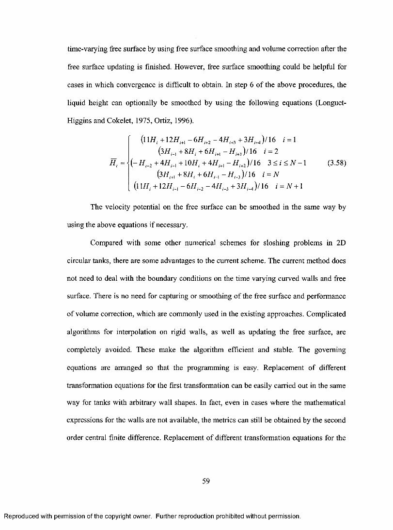
time-varying free surface by using free surface smoothing and volume correction after the
free surface updating is finished. However, free surface smoothing could be helpful for
cases in which convergence is difficult to obtain. In step 6 of the above procedures, the
liquid height can optionally be smoothed by using the following equations (Longuet-
Higgins and Cokelet, 1975, Ortiz, 1996).
(11H, + 12H,+1 — 6H,+2 — 4111+3 + 31/„+4 )/ 16 i =1
+ 8H, + 6H„+, — H,+3 )116 i = 2
+1011, + —H,+2)/16 3 i N —1
(3H,+, +8H, +6H,_, —H,_3 )/16 i =N
(11H, +12H,_ — 6111_2 — 4H1_3 + 3H,_4 )/16 i = N+1
(3.58)
The velocity potential on the free surface can be smoothed in the same way by
using the above equations if necessary.
Compared with some other numerical schemes for sloshing problems in 2D
circular tanks, there are some advantages to the current scheme. The current method does
not need to deal with the boundary conditions on the time varying curved walls and free
surface. There is no need for capturing or smoothing of the free surface and performance
of volume correction, which are commonly used in the existing approaches. Complicated
algorithms for interpolation on rigid walls, as well as updating the free surface, are
completely avoided. These make the algorithm efficient and stable. The governing
equations are arranged so that the programming is easy. Replacement of different
transformation equations for the first transformation can be easily carried out in the same
way for tanks with arbitrary wall shapes. In fact, even in cases where the mathematical
expressions for the walls are not available, the metrics can still be obtained by the second
order central finite difference. Replacement of different transformation equations for the
59
Reproduced with permission of the copyright owner. Further reproduction prohibited without permission.
time-varying free surface by using free surface smoothing and volume correction after the
free surface updating is finished. However, free surface smoothing could be helpful for
cases in which convergence is difficult to obtain. In step 6 o f the above procedures, the
liquid height can optionally be smoothed by using the following equations (Longuet-
Higgins and Cokelet, 1975, Ortiz, 1996).
( I I HI +12HM - 6 H M - 4 H M +3 HIJ / 1 6 i = 1
H, = <! ( - //,_2 + 4//,_, +107/,. + 4H m - H i+1)/16 3 < i < N - 1 (3.58)
(3W,.„+8ff,+6/fM- t f M)/16 i = N (l 1H, +12H,_, - 6H,_2 - 4 + 3//._4) /16 / = ,V +1
The velocity potential on the free surface can be smoothed in the same way by
using the above equations if necessary.
Compared with some other numerical schemes for sloshing problems in 2D
circular tanks, there are some advantages to the current scheme. The current method does
not need to deal with the boundary conditions on the time varying curved walls and free
surface. There is no need for capturing or smoothing of the free surface and performance
of volume correction, which are commonly used in the existing approaches. Complicated
algorithms for interpolation on rigid walls, as well as updating the free surface, are
completely avoided. These make the algorithm efficient and stable. The governing
equations are arranged so that the programming is easy. Replacement of different
transformation equations for the first transformation can be easily carried out in the same
way for tanks with arbitrary wall shapes. In fact, even in cases where the mathematical
expressions for the walls are not available, the metrics can still be obtained by the second
order central finite difference. Replacement o f different transformation equations for the
59
Reproduced with permission of the copyright owner. Further reproduction prohibited without permission.
third transformation can also be done without much extra modification needed for
program codes in adjusting the grids distribution.
3.5 Results and discussion
3.5.1 Sloshing in circular tanks under harmonic excitations with small amplitudes
In this section, the presented method is first used to simulate the sloshing problem
in a horizontal circular tank subjected to lateral harmonic motion with small amplitudes.
The tank is half-full. The displacement and acceleration of the tank are described by sine
functions.
D, = Do sin wt A, = —Dow2 sin ox (3.59)
In the above equations, Do = 0.002 is the amplitude of the tank displacement. co
is the excitation frequency.
To obtain necessary computational accuracy and solution convergence, numerical
trials have been carried out to find the proper grid size and time step. The grid size is
finally set to be 41x81 and the time step is set to be 0.005 for all cases in order to meet
the accuracy requirement, although coarser meshes and a larger time step can also be
used to get the same accuracy for cases where nonlinearity is weak or the excitation
frequencies are not close to the natural frequency. The convergence criterion of the
velocity potential is set to be 10-8.
Figure 3.5 presents the nondimensional liquid heights on the left and right walls
and at the middle point in a two-dimensional circular tank subjected to harmonic motion
under small amplitudes and different frequencies. It can be seen from Figure 3.5(a) that
the liquid heights on the walls are sine waves when the excitation frequency is far from
60
Reproduced with permission of the copyright owner. Further reproduction prohibited without permission.
third transformation can also be done without much extra modification needed for
program codes in adjusting the grids distribution.
3.5 Results and discussion
3.5.1 Sloshing in circular tanks under harmonic excitations with small amplitudes
In this section, the presented method is first used to simulate the sloshing problem
in a horizontal circular tank subjected to lateral harmonic motion with small amplitudes.
The tank is half-full. The displacement and acceleration of the tank are described by sine
functions.
Dx = D 0 sin cot Ax - -D 0 co2 sin cot (3.59)
In the above equations, D0 = 0.002 is the amplitude o f the tank displacement, co
is the excitation frequency.
To obtain necessary computational accuracy and solution convergence, numerical
trials have been carried out to find the proper grid size and time step. The grid size is
finally set to be 41x81 and the time step is set to be 0.005 for all cases in order to meet
the accuracy requirement, although coarser meshes and a larger time step can also be
used to get the same accuracy for cases where nonlinearity is weak or the excitation
frequencies are not close to the natural frequency. The convergence criterion o f the
velocity potential is set to be 10'8.
Figure 3.5 presents the nondimensional liquid heights on the left and right walls
and at the middle point in a two-dimensional circular tank subjected to harmonic motion
under small amplitudes and different frequencies. It can be seen from Figure 3.5(a) that
the liquid heights on the walls are sine waves when the excitation frequency is far from
60
Reproduced with permission of the copyright owner. Further reproduction prohibited without permission.
the natural frequency, which is 1.1644 or 1.169 (Lamb, 1945, Budiansky, 1960, and
Solaas and Faltinsen, 1997). When the excitation frequencies are close to the natural
frequency, i.e., Figure 3.5(c) and 3.5(e), the beat phenomena are obviously shown. When
the frequency is quite close to the natural frequency, i.e., Figure 3.5(d), the amplitude
grows monotonically with time. For other frequencies, i.e., Figure 3.5(b), the response is
the result of a combination of the excitation frequency and the natural frequency. For
most cases, the curves for the liquid height of the middle point at the free surface show
that the oscillation of the liquid height at the middle point is very small.
One criterion by which to verify the results is whether or not the conservation of
mass can be assured due to the assumption of incompressibility of liquid. The integral of
the free surface elevation over the free surface can be used for this purpose (Solaas and
Faltinsen, 1997). In the program, the volume error, Ve, is discretized on the free surface in
the a/3 coordinate system from the following expression.
Ve = 11 rida (3.60)
The volume errors corresponding to Figure 3.5 are obtained using the above
equation, and shown in Figure 3.6. Although smoothing of the free surface and volume
correction are not adopted in the current scheme, the results are quite satisfactory.
3.5.2 Sloshing in circular tanks under harmonic excitations with finite amplitude
near resonance
When the tank is subjected to a harmonic excitation with a finite amplitude near
resonance, the liquid behaviour is different because of the strong nonlinearity and
participation of higher modes. Figure 3.7 illustrates some free surface profiles from the
61
Reproduced with permission of the copyright owner. Further reproduction prohibited without permission.
the natural frequency, which is 1.1644 or 1.169 (Lamb, 1945, Budiansky, 1960, and
Solaas and Faltinsen, 1997). When the excitation frequencies are close to the natural
frequency, i.e., Figure 3.5(c) and 3.5(e), the beat phenomena are obviously shown. When
the frequency is quite close to the natural frequency, i.e., Figure 3.5(d), the amplitude
grows monotonically with time. For other frequencies, i.e., Figure 3.5(b), the response is
the result o f a combination of the excitation frequency and the natural frequency. For
most cases, the curves for the liquid height of the middle point at the free surface show
that the oscillation o f the liquid height at the middle point is very small.
One criterion by which to verify the results is whether or not the conservation of
mass can be assured due to the assumption o f incompressibility o f liquid. The integral of
the free surface elevation over the free surface can be used for this purpose (Solaas and
Faltinsen, 1997). In the program, the volume error, Ve, is discretized on the free surface in
the a p coordinate system from the following expression.
The volume errors corresponding to Figure 3.5 are obtained using the above
equation, and shown in Figure 3.6. Although smoothing of the free surface and volume
correction are not adopted in the current scheme, the results are quite satisfactory.
3.5.2 Sloshing in circular tanks under harmonic excitations with finite amplitude
near resonance
When the tank is subjected to a harmonic excitation with a finite amplitude near
resonance, the liquid behaviour is different because o f the strong nonlinearity and
participation o f higher modes. Figure 3.7 illustrates some free surface profiles from the
(3.60)
61
Reproduced with permission of the copyright owner. Further reproduction prohibited without permission.
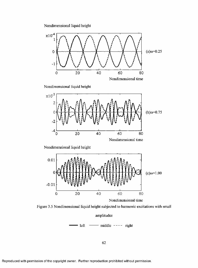
Nondimensional liquid height
x10-4
1
0
a 20 40 60 80
Nondimensional time
Nondimensional liquid height
X10-3
2
0
-2
-40
.•4 A • A t i I P e 1 I e I f I 1 % 1 li I 1i i I
%
I.I
I%
I. 1 I 1 it IA II II 4
20
Nondimensional liquid height
0 20
40
40
i al A f I I i 1 ir I i i I i i
1
I I it
Ir I
V 1 I i
I1C
60 80
Nondimensional time
60 80
Nondimensional time
(a)o)=0.25
(b)o)=0.75
(c)w=1.00
Figure 3.5 Nondimensional liquid height subjected to harmonic excitations with small
amplitudes
left middle - - - - right
62
Reproduced with permission of the copyright owner. Further reproduction prohibited without permission.
Nondimensional liquid height
0
1
40 60 800 20
(a)co=0.25
Nondimensional time
Nondimensional liquid height
■3xlO'
2
0V'
2 1 J
420 40 60 800
(b)co=0.75
Nondimensional time
Nondimensional liquid height
0.01
If
- 0.01
0 20 40 60 80
(c)<d=1.00
Nondimensional time
Figure 3.5 Nondimensional liquid height subjected to harmonic excitations with small
amplitudes
left m id d le right
62
Reproduced with permission of the copyright owner. Further reproduction prohibited without permission.
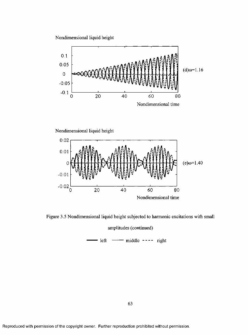
Nondimensional liquid height
0:1
0.05
0
-0.05
-0.1 0 2.0
Nondimensional liquid height
40 60 80
Nondimensional time
Nondimensional time
(d)w=1.16
(e)w=1.40
Figure 3.5 Nondimensional liquid height subjected to harmonic excitations with small
amplitudes (continued)
left middle - - - - right
63
Reproduced with permission of the copyright owner. Further reproduction prohibited without permission.
Nondimensional liquid height
0.1
0.05
-0.05
- 0.140 8060
Nondimensional time
(d)co=1.16
Nondimensional liquid height
0.02
0.01
0
- 0.01
- 0.02
M l ' A « A /
' A ' m l f t w m l !
h aAAAA
n W ' A l l fk •
i I V\ t 1 1 » 1 1 § f r A 1 I I VI il [ i M J ,1 / u> a i H. w ' M i
V VV“■ i
i l p U S I l !/ I Af i1
v - v y V s
•
11 1
0
(e)co=1.40
20 40 60 80Nondimensional time
Figure 3.5 Nondimensional liquid height subjected to harmonic excitations with small
amplitudes (continued)
left m id d le right
63
Reproduced with permission of the copyright owner. Further reproduction prohibited without permission.
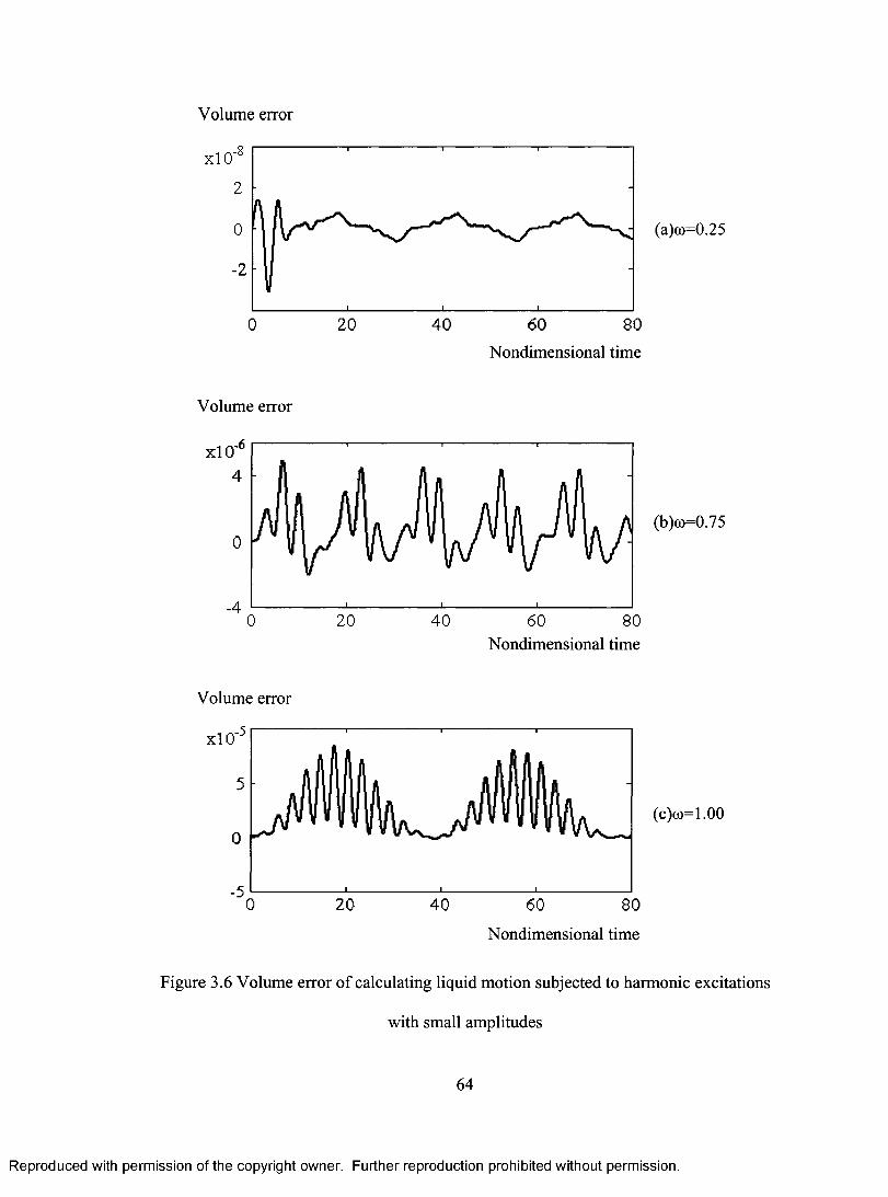
Volume error
x10-8
2
0
-2
0
Volume error
Volume error
20 40 60 80
Nondimensional time
20
20
40 60 80 Nondimensional time
40 60 80
Nondimensional time
(a)w=0.25
(b)co=0.75
(c)co=1.00
Figure 3.6 Volume error of calculating liquid motion subjected to harmonic excitations
with small amplitudes
64
Reproduced with permission of the copyright owner. Further reproduction prohibited without permission.
Volume error
2
(a)co=0.250
2
20 600 40 80
Nondimensional time
Volume error
xlO'
20 40 60 80 Nondimensional time
Volume error
xlO'
20 40 60 80
Nondimensional time
Figure 3.6 Volume error of calculating liquid motion subjected to harmonic excitations
with small amplitudes
64
Reproduced with permission of the copyright owner. Further reproduction prohibited without permission.
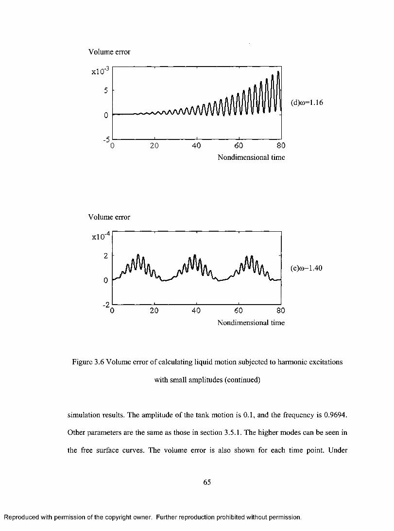
Volume error
20 40 60 80
Nondimensional time
Volume error
(e)co=1.40
Nondimensional time
Figure 3.6 Volume error of calculating liquid motion subjected to harmonic excitations
with small amplitudes (continued)
simulation results. The amplitude of the tank motion is 0.1, and the frequency is 0.9694.
Other parameters are the same as those in section 3.5.1. The higher modes can be seen in
the free surface curves. The volume error is also shown for each time point. Under
65
Reproduced with permission of the copyright owner. Further reproduction prohibited without permission.
Volume error
Nondimensional time
Volume error
(e)oo=1.40
60 80
Nondimensional time
Figure 3.6 Volume error o f calculating liquid motion subjected to harmonic excitations
with small amplitudes (continued)
simulation results. The amplitude of the tank motion is 0.1, and the frequency is 0.9694.
Other parameters are the same as those in section 3.5.1. The higher modes can be seen in
the free surface curves. The volume error is also shown for each time point. Under
65
Reproduced with permission of the copyright owner. Further reproduction prohibited without permission.
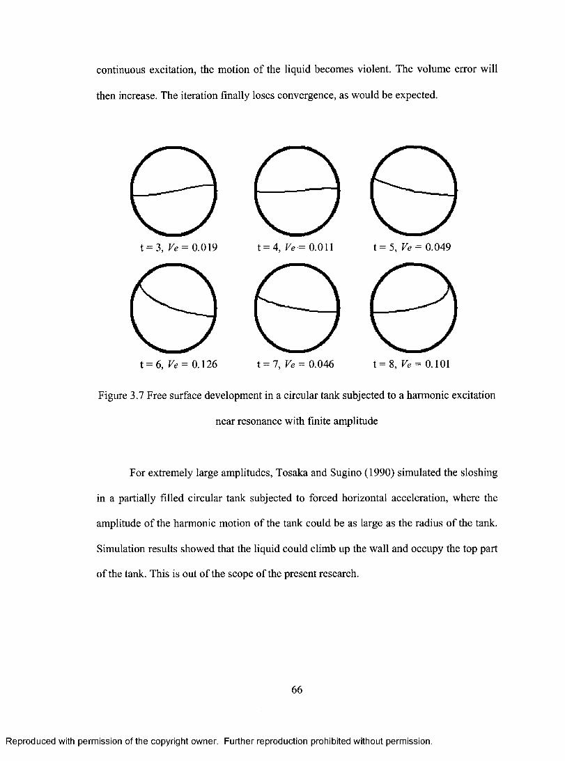
continuous excitation, the motion of the liquid becomes violent. The volume error will
then increase. The iteration finally loses convergence, as would be expected.
0 0 0 t = 3, Ve= 0.019 t = 4, Ve = 0.011 t= 5, Ve= 0.049
0 0 t = 6, Ve= 0.126 t = 7,Ve= 0.046 t = 8, Ve = 0.101
Figure 3.7 Free surface development in a circular tank subjected to a harmonic excitation
near resonance with finite amplitude
For extremely large amplitudes, Tosaka and Sugino (1990) simulated the sloshing
in a partially filled circular tank subjected to forced horizontal acceleration, where the
amplitude of the harmonic motion of the tank could be as large as the radius of the tank.
Simulation results showed that the liquid could climb up the wall and occupy the top part
of the tank. This is out of the scope of the present research.
66
Reproduced with permission of the copyright owner. Further reproduction prohibited without permission.
continuous excitation, the motion of the liquid becomes violent. The volume error will
then increase. The iteration finally loses convergence, as would be expected.
t = 4, V e - = 0.011 t = 5, V e = 0.049t = 3, V e = 0.019
t = 7 , V e = 0.046 t = 8, V e ~ 0.101t = 6, V e = 0.126
Figure 3.7 Free surface development in a circular tank subjected to a harmonic excitation
near resonance with finite amplitude
For extremely large amplitudes, Tosaka and Sugino (1990) simulated the sloshing
in a partially filled circular tank subjected to forced horizontal acceleration, where the
amplitude o f the harmonic motion o f the tank could be as large as the radius o f the tank.
Simulation results showed that the liquid could climb up the wall and occupy the top part
o f the tank. This is out of the scope of the present research.
66
Reproduced with permission of the copyright owner. Further reproduction prohibited without permission.
3.5.3 Transient liquid oscillations in circular tanks
In most applications of road transportation, the input accelerations do not
necessarily need to be harmonic. To study the transient liquid responses in circular tanks,
three different input types are considered, and sloshing problems under these input types
are simulated. The system parameters are the same as those in Section 3.4.1. The first
type is shown in Figure 3.8(a), where the lateral acceleration applied builds up to its final
steady value, Ao, in an input time, to. This can be used to simulate the acceleration input
for a liquid vehicle during a turning operation.
Figure 3.9 shows the nondimensional liquid height on the right wall of a circular
tank during turning subjected to different steady accelerations with the same input time,
10.0. It can be found that the liquid height decreases during the input time. After the final
steady acceleration is reached, the liquid heights begin to oscillate around their
equilibrium positions, which correspond to the static positions that can be obtained by
isobars. The oscillation amplitude increases with the increase in the steady acceleration.
Therefore, the forces and moments on the tank and supporting structures caused by
turning would also have oscillatory characteristics, which cannot be ignored when
structural integrity and fatigue are considered, especially under large turning
accelerations. When the lateral acceleration for the turning operation for liquid cargo
vehicles is higher than 0.3g, it is very possible that rollover of the partially filled vehicle
could happen, and the conditions for sloshing problems will not exist. Calculations also
show that when the input acceleration is higher than 0.3g, the convergence of the iteration
can become very slow and difficult, which is basically caused by the application of the
67
Reproduced with permission of the copyright owner. Further reproduction prohibited without permission.
3.5.3 Transient liquid oscillations in circular tanks
In most applications of road transportation, the input accelerations do not
necessarily need to be harmonic. To study the transient liquid responses in circular tanks,
three different input types are considered, and sloshing problems under these input types
are simulated. The system parameters are the same as those in Section 3.4.1. The first
type is shown in Figure 3.8(a), where the lateral acceleration applied builds up to its final
steady value, A o , in an input time, t o - This can be used to simulate the acceleration input
for a liquid vehicle during a turning operation.
Figure 3.9 shows the nondimensional liquid height on the right wall o f a circular
tank during turning subjected to different steady accelerations with the same input time,
10.0. It can be found that the liquid height decreases during the input time. After the final
steady acceleration is reached, the liquid heights begin to oscillate around their
equilibrium positions, which correspond to the static positions that can be obtained by
isobars. The oscillation amplitude increases with the increase in the steady acceleration.
Therefore, the forces and moments on the tank and supporting structures caused by
turning would also have oscillatory characteristics, which cannot be ignored when
structural integrity and fatigue are considered, especially under large turning
accelerations. When the lateral acceleration for the turning operation for liquid cargo
vehicles is higher than 0.3g, it is very possible that rollover o f the partially filled vehicle
could happen, and the conditions for sloshing problems will not exist. Calculations also
show that when the input acceleration is higher than 0.3g, the convergence of the iteration
can become very slow and difficult, which is basically caused by the application o f the
67
Reproduced with permission of the copyright owner. Further reproduction prohibited without permission.
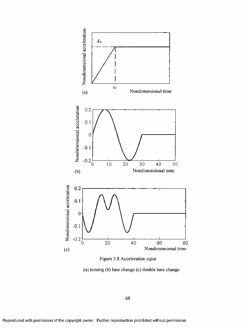
Non
dim
ensi
onal
acc
eler
atio
n
Non
dim
ensi
onal
acc
eler
atio
n
(b)
0.2
0.1
-0.1
to Nondimensional time
-0.2 0
0.2
0.1
0
-0.1
-0.2. 0
(c)
10 20 30 40 50 Nondimensional time
20 40 60 80 Nondimensional time
Figure 3.8 Acceleration input
(a) turning (b) lane change (c) double lane change
68
Reproduced with permission of the copyright owner. Further reproduction prohibited without permission.
o
<D
CTJfio
t oNondimensional time
2 0.2
8 0.1
I °Wge - o . ico
£ - 0.230 40 5
Nondimensional time
I 0.2
^ rv§ 0C/3
I -0 -1■oco£ - 0.2
4020Nondimensional time
Figure 3.8 Acceleration input
(a) turning (b) lane change (c) double lane change
68
Reproduced with permission of the copyright owner. Further reproduction prohibited without permission.
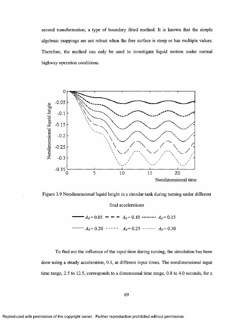
second transformation, a type of boundary fitted method. It is known that the simple
algebraic mappings are not robust when the free surface is steep or has multiple values.
Therefore, the method can only be used to investigate liquid motion under normal
highway operation conditions.
Non
dim
ensi
onal
liq
uid
heig
ht
0
-0.05
-0.1
-0.15
-0.2
-0.25
-0.3
-0.35 0 5 10 15 20
Nondimensional time
Figure 3.9 Nondimensional liquid height in a circular tank during turning under different
final accelerations
Ao= 0 .05 — -- — A0 = 0 .10 Ao= 0.15
Ao — 0.20 Ao — 0.25 Ao = 0.30
To find out the influence of the input time during turning, the simulation has been
done using a steady acceleration, 0.1, at different input times. The nondimensional input
time range, 2.5 to 12.5, corresponds to a dimensional time range, 0.8 to 4.0 seconds, for a
69
Reproduced with permission of the copyright owner. Further reproduction prohibited without permission.
second transformation, a type of boundary fitted method. It is known that the simple
algebraic mappings are not robust when the free surface is steep or has multiple values.
Therefore, the method can only be used to investigate liquid motion under normal
highway operation conditions.
-0.05
- 0.1
-0.15cd G o
• (/> ca.£ -0.25CO£ -0.3
- 0.2
-0.3520
Nondimensional time
Figure 3.9 Nondimensional liquid height in a circular tank during turning under different
final accelerations
A o = 0 . 0 5 ------------------0.10 A o = 0.15
A o ~ 0 .2 0 -------- A 0 = 0.25 ............ ^ 0=0.30
To find out the influence of the input time during turning, the simulation has been
done using a steady acceleration, 0.1, at different input times. The nondimensional input
time range, 2.5 to 12.5, corresponds to a dimensional time range, 0.8 to 4.0 seconds, for a
69
Reproduced with permission of the copyright owner. Further reproduction prohibited without permission.
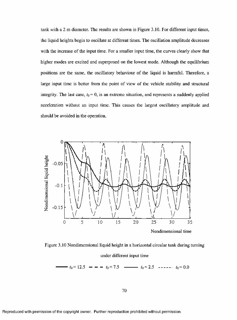
tank with a 2 m diameter. The results are shown in Figure 3.10. For different input times,
the liquid heights begin to oscillate at different times. The oscillation amplitude decreases
with the increase of the input time. For a smaller input time, the curves clearly show that
higher modes are excited and superposed on the lowest mode. Although the equilibrium
positions are the same, the oscillatory behaviour of the liquid is harmful. Therefore, a
large input time is better from the point of view of the vehicle stability and structural
integrity. The last case, to = 0, is an extreme situation, and represents a suddenly applied
acceleration without an input time. This causes the largest oscillatory amplitude and
should be avoided in the operation.
Non
dim
ensi
onal
liq
uid
heig
ht
0
-0.05
-0.1
-0.15
0 5 10 15 20 25 30 35
Nondimensional time
Figure 3.10 Nondimensional liquid height in a horizontal circular tank during turning
under different input time
to = 12.5 — — — to = 7.5 to — 2.5 to = 0.0
70
Reproduced with permission of the copyright owner. Further reproduction prohibited without permission.
tank with a 2 m diameter. The results are shown in Figure 3.10. For different input times,
the liquid heights begin to oscillate at different times. The oscillation amplitude decreases
with the increase o f the input time. For a smaller input time, the curves clearly show that
higher modes are excited and superposed on the lowest mode. Although the equilibrium
positions are the same, the oscillatory behaviour of the liquid is harmful. Therefore, a
large input time is better from the point of view of the vehicle stability and structural
integrity. The last case, to = 0, is an extreme situation, and represents a suddenly applied
acceleration without an input time. This causes the largest oscillatory amplitude and
should be avoided in the operation.
2 -0.05rs
I -0 1C/3
C3us
-3
I -°15
0 5 10 15 20 25 30 35
Nondimensional time
Figure 3.10 Nondimensional liquid height in a horizontal circular tank during turning
under different input time
to = 12.5 — — - t0 =7.5 ---------- to =2.5 t0= 0 .0
70
Reproduced with permission of the copyright owner. Further reproduction prohibited without permission.
The other two input types for transient response study are shown in Figure 3.8 (b)
and (c). In Figure 3.8 (b), the input acceleration is expressed using a single period sine
function. This is used to simulate the lateral acceleration input for a road vehicle during a
lane change operation. In Figure 3.8 (c), the input acceleration is described using a
combination of sine functions, which can approximate the lateral acceleration input for a
road vehicle during a double lane change operation. The wave developments under these
two types of input are shown in Figure 3.11(a) and Figure 3.11 (b). Since the input
frequency is much smaller than the liquid sloshing modes, the wave in the tank develops
in step with the input acceleration. The natural modes are actuated and shown in the
figures. After the operation is finished, the liquid height oscillates around the equilibrium
position. Because the liquid in the double lane change operation is actuated much more
than in the lane change, the oscillation amplitude after the double lane change is much
larger than after the lane change, even though the amplitude of the input acceleration is
larger in the lane change.
It is interesting that in some early vehicle stability researches, liquid motion in
tanks was sometimes modeled by mass centre models, which assumed that the liquid kept
a perfectly inclined flat surface during operations. This assumption may cause two
concerns. First, for many operations, the free surfaces have complicated shapes and
cannot be simply considered as a straight line. Also, the mass centre of the liquid bulk
would be different. This phenomenon has been shown numerically (Popov et al, 1993b),
as well as experimentally (Rakheja et al, 1992). Second, even the liquid motion is
approximated by the first natural liquid mode, for which the free surface could be
approximated by a straight line, the dynamic feature of liquid motion makes the flat free
71
Reproduced with permission of the copyright owner. Further reproduction prohibited without permission.
The other two input types for transient response study are shown in Figure 3.8 (b)
and (c). In Figure 3.8 (b), the input acceleration is expressed using a single period sine
function. This is used to simulate the lateral acceleration input for a road vehicle during a
lane change operation. In Figure 3.8 (c), the input acceleration is described using a
combination o f sine functions, which can approximate the lateral acceleration input for a
road vehicle during a double lane change operation. The wave developments under these
two types of input are shown in Figure 3.11(a) and Figure 3.11 (b). Since the input
frequency is much smaller than the liquid sloshing modes, the wave in the tank develops
in step with the input acceleration. The natural modes are actuated and shown in the
figures. After the operation is finished, the liquid height oscillates around the equilibrium
position. Because the liquid in the double lane change operation is actuated much more
than in the lane change, the oscillation amplitude after the double lane change is much
larger than after the lane change, even though the amplitude of the input acceleration is
larger in the lane change.
It is interesting that in some early vehicle stability researches, liquid motion in
tanks was sometimes modeled by mass centre models, which assumed that the liquid kept
a perfectly inclined flat surface during operations. This assumption may cause two
concerns. First, for many operations, the free surfaces have complicated shapes and
cannot be simply considered as a straight line. Also, the mass centre o f the liquid bulk
would be different. This phenomenon has been shown numerically (Popov et al, 1993b),
as well as experimentally (Rakheja et al, 1992). Second, even the liquid motion is
approximated by the first natural liquid mode, for which the free surface could be
approximated by a straight line, the dynamic feature of liquid motion makes the flat free
71
Reproduced with permission of the copyright owner. Further reproduction prohibited without permission.
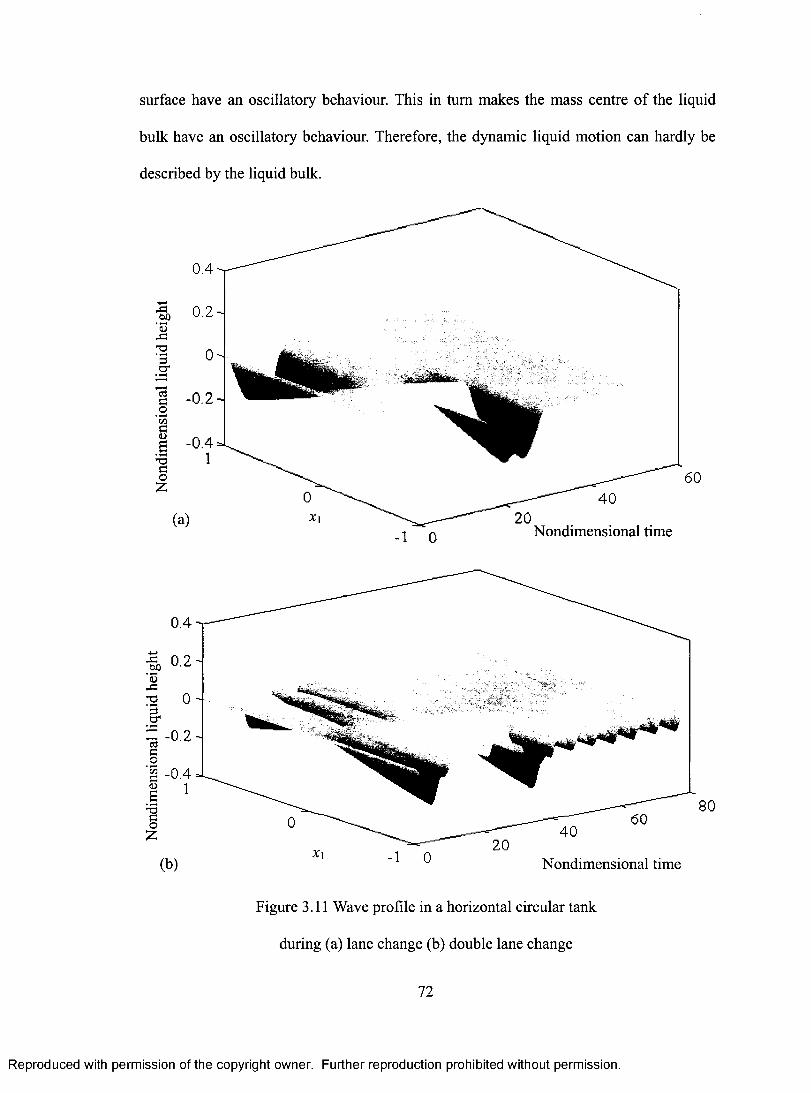
surface have an oscillatory behaviour. This in turn makes the mass centre of the liquid
bulk have an oscillatory behaviour. Therefore, the dynamic liquid motion can hardly be
described by the liquid bulk. N
ondi
men
sion
al l
iqui
d he
ight
(a)
0 Xi
Xi 20
20 40
Nondimensional time
40
Nondimensional time
Figure 3.11 Wave profile in a horizontal circular tank
during (a) lane change (b) double lane change
72
60
80
Reproduced with permission of the copyright owner. Further reproduction prohibited without permission.
surface have an oscillatory behaviour. This in turn makes the mass centre o f the liquid
bulk have an oscillatory behaviour. Therefore, the dynamic liquid motion can hardly be
described by the liquid bulk.
-1 0 Nondimensional time
§ -0.4
Nondimensional time
Figure 3.11 Wave profile in a horizontal circular tank
during (a) lane change (b) double lane change
72
Reproduced with permission of the copyright owner. Further reproduction prohibited without permission.
In the above simulations of the transient response of liquids, it is shown that the
oscillatory motions of liquids continue due to the lack of damping in the current study. In
a real situation, the liquid will eventually calm down if there is no new excitation. The
time required for the transient effect to die out depends on the viscosity of the liquid
being carried.
The importance of viscosity in the liquid sloshing problems depends on the
different excitation types. The effect of viscosity is more significant near tank walls and
near a resonant frequency during liquid sloshing. The influence of fluid viscosity can be
considered without any approximation if the sloshing problems are described by the
Navier-Stokes equations. For example, a straightforward investigation was conducted by
Popov et al (1993b) to study the influence of liquid viscosity on the dynamics of road
tanks subjected to suddenly applied lateral accelerations, based on the Navier-Stokes
equations. The effect was shown in terms of the Reynolds number. It was found that the
Re number had no influence on the magnitudes and frequencies of the sloshing
parameters in the range 107-105. In the range 105-103, the influence was rather small. For
the range Re < 103, the difference in amplitudes and frequencies rapidly increased in such
a way that more viscous liquids vibrated more slowly, with a smaller amplitude and with
stronger decay. It was concluded that for the majority of practical cases, covered by Re >
105, the main sloshing parameters, such as the magnitudes and frequencies of the sloshing
forces and moments, were almost independent of the Re number (Popov et al, 1993b).
However, when the sloshing problems are modeled by the potential flow theory,
the liquid viscosity cannot be directly included. As long as the tank holding the liquid is
smooth inside and not very small, viscosity plays a minor role in determining the sloshing
73
Reproduced with permission of the copyright owner. Further reproduction prohibited without permission.
In the above simulations of the transient response of liquids, it is shown that the
oscillatory motions of liquids continue due to the lack of damping in the current study. In
a real situation, the liquid will eventually calm down if there is no new excitation. The
time required for the transient effect to die out depends on the viscosity o f the liquid
being carried.
The importance of viscosity in the liquid sloshing problems depends on the
different excitation types. The effect of viscosity is more significant near tank walls and
near a resonant frequency during liquid sloshing. The influence o f fluid viscosity can be
considered without any approximation if the sloshing problems are described by the
Navier-Stokes equations. For example, a straightforward investigation was conducted by
Popov et al (1993b) to study the influence o f liquid viscosity on the dynamics o f road
tanks subjected to suddenly applied lateral accelerations, based on the Navier-Stokes
equations. The effect was shown in terms of the Reynolds number. It was found that the
Re number had no influence on the magnitudes and frequencies o f the sloshing
parameters in the range 107-105. In the range 105-103, the influence was rather small. For
the range Re < 103, the difference in amplitudes and frequencies rapidly increased in such
a way that more viscous liquids vibrated more slowly, with a smaller amplitude and with
stronger decay. It was concluded that for the majority o f practical cases, covered by Re >
105, the main sloshing parameters, such as the magnitudes and frequencies o f the sloshing
forces and moments, were almost independent o f the Re number (Popov et al, 1993b).
However, when the sloshing problems are modeled by the potential flow theory,
the liquid viscosity cannot be directly included. As long as the tank holding the liquid is
smooth inside and not very small, viscosity plays a minor role in determining the sloshing
73
Reproduced with permission of the copyright owner. Further reproduction prohibited without permission.
behaviour. Hence it is usually neglected without sacrificing the essential features of the
phenomenon. In cases where the damping effect is expected in the simulation, a
commonly adopted method is to introduce a dissipation mechanism into the description
of the fluid instead of solving the full Navier-Stokes equations. By introducing a fictitious
term into the Euler equation, a modified Bernoulli equation can be obtained with a
modified Rayleigh damping term (Faltinsen, 1974 and Faltinsen, 1978). In this way, the
dynamic condition on the free surface, i.e., Eq. (3.12), can be modified as:
act ,__1 aq3N2at 2 ax
(a1
2— — Axx — pc,
a (3.61)
The modified Rayleigh damping term, ,uco, is included to simulate the viscosity of the
liquid in order to study the damping effect in the liquid motion. The way to decide the
value of p can be found in Faltinsen (1974), Faltinsen (1978) and Ortiz and Barhorst
(1998).
3.6 Liquid motion in 2D elliptical tanks
3.6.1 Statement of liquid motion in 2D elliptical tanks
Tanks with elliptical cross sections are also widely used in road transportation
industry. There are very few reports on sloshing studies for this specific configuration in
the current literature. The first natural mode of liquid motion was investigated by Salem
(2000) using an equivalent mechanical pendulum by linearization under the assumption
of a flat free surface and small oscillation angle. The analogy was established in the
transverse direction and therefore had a 2D solution. Liquid motion under finite
excitations in the roll plane and 3D liquid behaviour were not considered.
74
Reproduced with permission of the copyright owner. Further reproduction prohibited without permission.
behaviour. Hence it is usually neglected without sacrificing the essential features o f the
phenomenon. In cases where the damping effect is expected in the simulation, a
commonly adopted method is to introduce a dissipation mechanism into the description
o f the fluid instead of solving the full Navier-Stokes equations. By introducing a fictitious
term into the Euler equation, a modified Bernoulli equation can be obtained with a
modified Rayleigh damping term (Faltinsen, 1974 and Faltinsen, 1978). In this way, the
dynamic condition on the free surface, i.e., Eq. (3.12), can be modified as:
dtpdt
r dcp^ \ d x j
+r dcpv
- £ - A xx-n<p (3.61)
The modified Rayleigh damping term, /J.(p, is included to simulate the viscosity o f the
liquid in order to study the damping effect in the liquid motion. The way to decide the
value o f n can be found in Faltinsen (1974), Faltinsen (1978) and Ortiz and Barhorst
(1998).
3.6 Liquid motion in 2D elliptical tanks
3.6.1 Statement of liquid motion in 2D elliptical tanks
Tanks with elliptical cross sections are also widely used in road transportation
industry. There are very few reports on sloshing studies for this specific configuration in
the current literature. The first natural mode of liquid motion was investigated by Salem
(2000) using an equivalent mechanical pendulum by linearization under the assumption
o f a flat free surface and small oscillation angle. The analogy was established in the
transverse direction and therefore had a 2D solution. Liquid motion under finite
excitations in the roll plane and 3D liquid behaviour were not considered.
74
Reproduced with permission of the copyright owner. Further reproduction prohibited without permission.
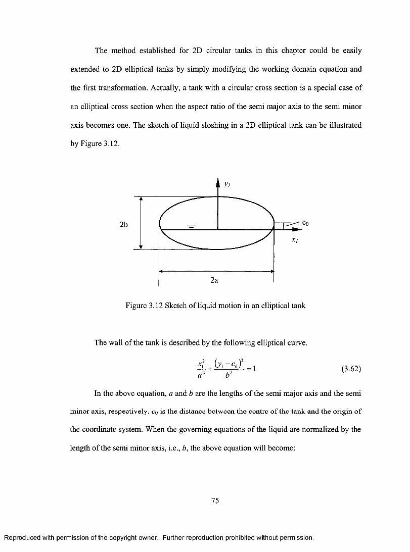
The method established for 2D circular tanks in this chapter could be easily
extended to 2D elliptical tanks by simply modifying the working domain equation and
the first transformation. Actually, a tank with a circular cross section is a special case of
an elliptical cross section when the aspect ratio of the semi major axis to the semi minor
axis becomes one. The sketch of liquid sloshing in a 2D elliptical tank can be illustrated
by Figure 3.12.
2b
Figure 3.12 Sketch of liquid motion in an elliptical tank
The wall of the tank is described by the following elliptical curve.
2 +
1 x l VI b - CO )2 =1a 2 2
(3.62)
In the above equation, a and b are the lengths of the semi major axis and the semi
minor axis, respectively. co is the distance between the centre of the tank and the origin of
the coordinate system. When the governing equations of the liquid are normalized by the
length of the semi minor axis, i.e., b, the above equation will become:
75
Reproduced with permission of the copyright owner. Further reproduction prohibited without permission.
The method established for 2D circular tanks in this chapter could be easily
extended to 2D elliptical tanks by simply modifying the working domain equation and
the first transformation. Actually, a tank with a circular cross section is a special case of
an elliptical cross section when the aspect ratio of the semi major axis to the semi minor
axis becomes one. The sketch of liquid sloshing in a 2D elliptical tank can be illustrated
by Figure 3.12.
2b
Figure 3.12 Sketch of liquid motion in an elliptical tank
The wall of the tank is described by the following elliptical curve.
i L + f o - C o ) =1 (3 62)a b
In the above equation, a and b are the lengths o f the semi major axis and the semi
minor axis, respectively, co is the distance between the centre of the tank and the origin of
the coordinate system. When the governing equations o f the liquid are normalized by the
length of the semi minor axis, i.e., b, the above equation will become:
75
Reproduced with permission of the copyright owner. Further reproduction prohibited without permission.
2 X 2 ± (y — c0 )2 =1
a (3.63)
Note that a and co in this equation are the nondimensional quantities that are normalized
by b. The first transformation will then be performed using the following equations.
a= x
= Y (y — co )2
(3.64)
The singularity at the bottom point will be treated in the same way used for a
circular tank. By using the same method for the other two coordinate transformations and
the same numerical procedures, the sloshing problems in elliptical tanks can be solved
without any difficulties.
3.6.2 Natural frequencies
The natural frequencies of liquid sloshing in circular tanks have been well
evaluated by several researchers (Budiansky, 1960, McIver, 1989) under different fill
levels. However, there is no detailed study on the natural frequencies of liquid motion in
elliptical tanks. In this section, the natural frequencies in an elliptical tank are calculated
to verify the method developed in this chapter. When the natural frequency problem is to
be solved, the linearized Bernoulli equation on the free surface can be obtained as follows
(Budiansky, 1960).
a =
ay (3.65)
In the above equation, xis the eigenvalue. The frequency is to be solved using:
(3.66)
76
Reproduced with permission of the copyright owner. Further reproduction prohibited without permission.
Note that a and Co in this equation are the nondimensional quantities that are normalized
by b. The first transformation will then be performed using the following equations.
The singularity at the bottom point will be treated in the same way used for a
circular tank. By using the same method for the other two coordinate transformations and
the same numerical procedures, the sloshing problems in elliptical tanks can be solved
without any difficulties.
3.6.2 Natural frequencies
The natural frequencies o f liquid sloshing in circular tanks have been well
evaluated by several researchers (Budiansky, 1960, Mclver, 1989) under different fill
levels. However, there is no detailed study on the natural frequencies o f liquid motion in
elliptical tanks. In this section, the natural frequencies in an elliptical tank are calculated
to verify the method developed in this chapter. When the natural frequency problem is to
be solved, the linearized Bernoulli equation on the free surface can be obtained as follows
(Budiansky, 1960).
In the above equation, k is the eigenvalue. The frequency is to be solved using:
x (3.64)a =
(3.66)
76
Reproduced with permission of the copyright owner. Further reproduction prohibited without permission.
Since the natural frequency problem is fixed in the domain which the liquid
initially occupies, only the first and the third transformations in this chapter are used for
the linearized Bernoulli equation on the free surface. Discretization of the governing
equations leads to a generalized eigenvalue problem.
Tx = /Mx (3.67)
In the above equations, Wand 0 are coefficient matrices and x is the eigenvector.
To verify the method developed in this chapter for the eigenvalue problem, the first three
eigenvalues for a half-filled circular tank have been solved by trying different mesh sizes.
Figure 3.13 illustrates the eigenvalue results calculated by different grid numbers in both
horizontal and vertical directions. The results show that the eigenvalues eventually
converge when the cell numbers are 40x80. The eigenvalues converge to the values
calculated by other methods, which can be shown by the last points (McIver, 1989) for
corresponding curves.
Eigenvalues in a partially filled circular tank at different fill levels have been
solved in the same way. The results for a tank of unit radius are shown in Figure 3.14.
The first and third eigenvalues are the first and second antisymmetrical modes. The
second eigenvalue is the first symmetrical mode. The eigenvalues for points on the
dashed line in this figure are taken from McIver (1989), in which the linearized wave
theory was used to solve the eigenvalues of free oscillations numerically by integral
equations in a bipolar coordinate system for circular tanks. The eigenvalues for points on
the solid line are calculated using the current method. It can be seen that the results in this
study are in good agreement with the results from McIver (1989).
77
Reproduced with permission of the copyright owner. Further reproduction prohibited without permission.
Since the natural frequency problem is fixed in the domain which the liquid
initially occupies, only the first and the third transformations in this chapter are used for
the linearized Bernoulli equation on the free surface. Discretization o f the governing
equations leads to a generalized eigenvalue problem.
V Z = «®Z (3.67)
In the above equations, W and <9 are coefficient matrices and x is the eigenvector.
To verify the method developed in this chapter for the eigenvalue problem, the first three
eigenvalues for a half-filled circular tank have been solved by trying different mesh sizes.
Figure 3.13 illustrates the eigenvalue results calculated by different grid numbers in both
horizontal and vertical directions. The results show that the eigenvalues eventually
converge when the cell numbers are 40x80. The eigenvalues converge to the values
calculated by other methods, which can be shown by the last points (Mclver, 1989) for
corresponding curves.
Eigenvalues in a partially filled circular tank at different fill levels have been
solved in the same way. The results for a tank o f unit radius are shown in Figure 3.14.
The first and third eigenvalues are the first and second antisymmetrical modes. The
second eigenvalue is the first symmetrical mode. The eigenvalues for points on the
dashed line in this figure are taken from Mclver (1989), in which the linearized wave
theory was used to solve the eigenvalues of free oscillations numerically by integral
equations in a bipolar coordinate system for circular tanks. The eigenvalues for points on
the solid line are calculated using the current method. It can be seen that the results in this
study are in good agreement with the results from Mclver (1989).
77
Reproduced with permission of the copyright owner. Further reproduction prohibited without permission.
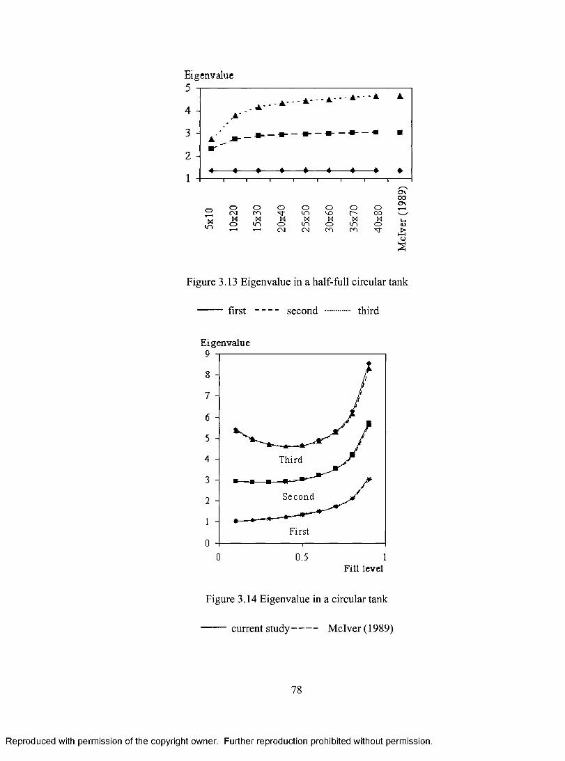
Eigenvalue 5
4 -
3 -
2 -
1
_ A' - A —
AL .... —_ 41— -- ill— -- il— -- il— -- 0— -- 0
E"'
A
•
• 4 0 • 0 4 4 • 4
,---, Cr% CO
% 0 0 0 0 0 0 0 ,—. CV c Sr Le) ko r- co ,_, N N N N N N N t_.
0 4-1 0 Lr-, c, in c> a) •—• ,—. CV CV Or) c ,cr
1---1 0
Figure 3.13 Eigenvalue in a half-full circular tank
first - - - - second third
Ei genvalue 9
Figure 3.14 Eigenvalue in a circular tank
current study---- McIver (1989)
78
Reproduced with permission of the copyright owner. Further reproduction prohibited without permission.
Eigenvalue5
4
3
2
1C\00
o o o O o o oCM CO M" n kO r- 00
K N xO m O m o m o1 i—■1 CM CM Ci
3
Figure 3.13 Eigenvalue in a half-full circular tank
f i r s t second .......... third
Eigenvalue9
8
7
6
5
4 Third
3
Second2
First0
0 0.5Fill level
Figure 3.14 Eigenvalue in a circular tank
current study M clver(1989)
78
Reproduced with permission of the copyright owner. Further reproduction prohibited without permission.
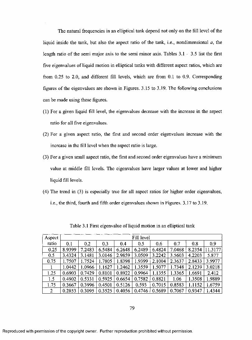
The natural frequencies in an elliptical tank depend not only on the fill level of the
liquid inside the tank, but also the aspect ratio of the tank, i.e., nondimensional a, the
length ratio of the semi major axis to the semi minor axis. Tables 3.1 - 3.5 list the first
five eigenvalues of liquid motion in elliptical tanks with different aspect ratios, which are
from 0.25 to 2.0, and different fill levels, which are from 0.1 to 0.9. Corresponding
figures of the eigenvalues are shown in Figures. 3.15 to 3.19. The following conclusions
can be made using these figures.
(1) For a given liquid fill level, the eigenvalues decrease with the increase in the aspect
ratio for all five eigenvalues.
(2) For a given aspect ratio, the first and second order eigenvalues increase with the
increase in the fill level when the aspect ratio is large.
(3) For a given small aspect ratio, the first and second order eigenvalues have a minimum
value at middle fill levels. The eigenvalues have larger values at lower and higher
liquid fill levels.
(4) The trend in (3) is especially true for all aspect ratios for higher order eigenvalues,
i.e., the third, fourth and fifth order eigenvalues shown in Figures. 3.17 to 3.19.
Table 3.1 First eigenvalue of liquid motion in an elliptical tank
Aspect ratio
Fill level 0.1 0.2 0.3 0.4 0.5 0.6 0.7 0.8 0.9
0.25 8.9399 7.2483 6.5484 6.2648 6.2489 6.4824 7.0468 8.2354 11.3177 0.5 3.4324 3.1481 3.0146 2.9859 3.0509 3.2242 3.5603 4.2203 5.877 0.75 1.7507 1.7524 1.7805 1.8398 1.9399 2.1004 2.3637 2.8433 3.9977
1 1.0442 1.0966 1.1627 1.2462 1.3559 1.5077 1.7348 2.1239 3.0218 1.25 0.6903 0.7429 0.8101 0.8922 0.9964 1.1355 1.3365 1.6691 2.412 1.5 0.4902 0.5331 0.5925 0.6654 0.7582 0.8821 1.06 1.3508 1.9889 1.75 0.3667 0.3996 0.4501 0.5126 0.593 0.7015 0.8583 1.1152 1.6759
2 0.2853 0.3095 0.3525 0.4056 0.4746 0.5689 0.7067 0.9347 1.4344
79
Reproduced with permission of the copyright owner. Further reproduction prohibited without permission.
The natural frequencies in an elliptical tank depend not only on the fill level of the
liquid inside the tank, but also the aspect ratio o f the tank, i.e., nondimensional a, the
length ratio o f the semi major axis to the semi minor axis. Tables 3.1 - 3.5 list the first
five eigenvalues o f liquid motion in elliptical tanks with different aspect ratios, which are
from 0.25 to 2.0, and different fill levels, which are from 0.1 to 0.9. Corresponding
figures o f the eigenvalues are shown in Figures. 3.15 to 3.19. The following conclusions
can be made using these figures.
(1) For a given liquid fill level, the eigenvalues decrease with the increase in the aspect
ratio for all five eigenvalues.
(2) For a given aspect ratio, the first and second order eigenvalues increase with the
increase in the fill level when the aspect ratio is large.
(3) For a given small aspect ratio, the first and second order eigenvalues have a minimum
value at middle fill levels. The eigenvalues have larger values at lower and higher
liquid fill levels.
(4) The trend in (3) is especially true for all aspect ratios for higher order eigenvalues,
i.e., the third, fourth and fifth order eigenvalues shown in Figures. 3.17 to 3.19.
Table 3.1 First eigenvalue of liquid motion in an elliptical tank
Aspectratio
Fill level0.1 0.2 0.3 0.4 0.5 0.6 0.7 0.8 0.9
0.25 8.9399 7.2483 6.5484 6.2648 6.2489 6.4824 7.0468 8.2354 11.31770.5 3.4324 3.1481 3.0146 2.9859 3.0509 3.2242 3.5603 4.2203 5.877
0.75 1.7507 1.7524 1.7805 1.8398 1.9399 2.1004 2.3637 2.8433 3.99771 1.0442 1.0966 1.1627 1.2462 1.3559 1.5077 1.7348 2.1239 3.0218
1.25 0.6903 0.7429 0.8101 0.8922 0.9964 1.1355 1.3365 1.6691 2.4121.5 0.4902 0.5331 0.5925 0.6654 0.7582 0.8821 1.06 1.3508 1.9889
1.75 0.3667 0.3996 0.4501 0.5126 0.593 0.7015 0.8583 1.1152 1.67592 0.2853 0.3095 0.3525 0.4056 0.4746 0.5689 0.7067 0.9347 1.4344
79
Reproduced with permission of the copyright owner. Further reproduction prohibited without permission.
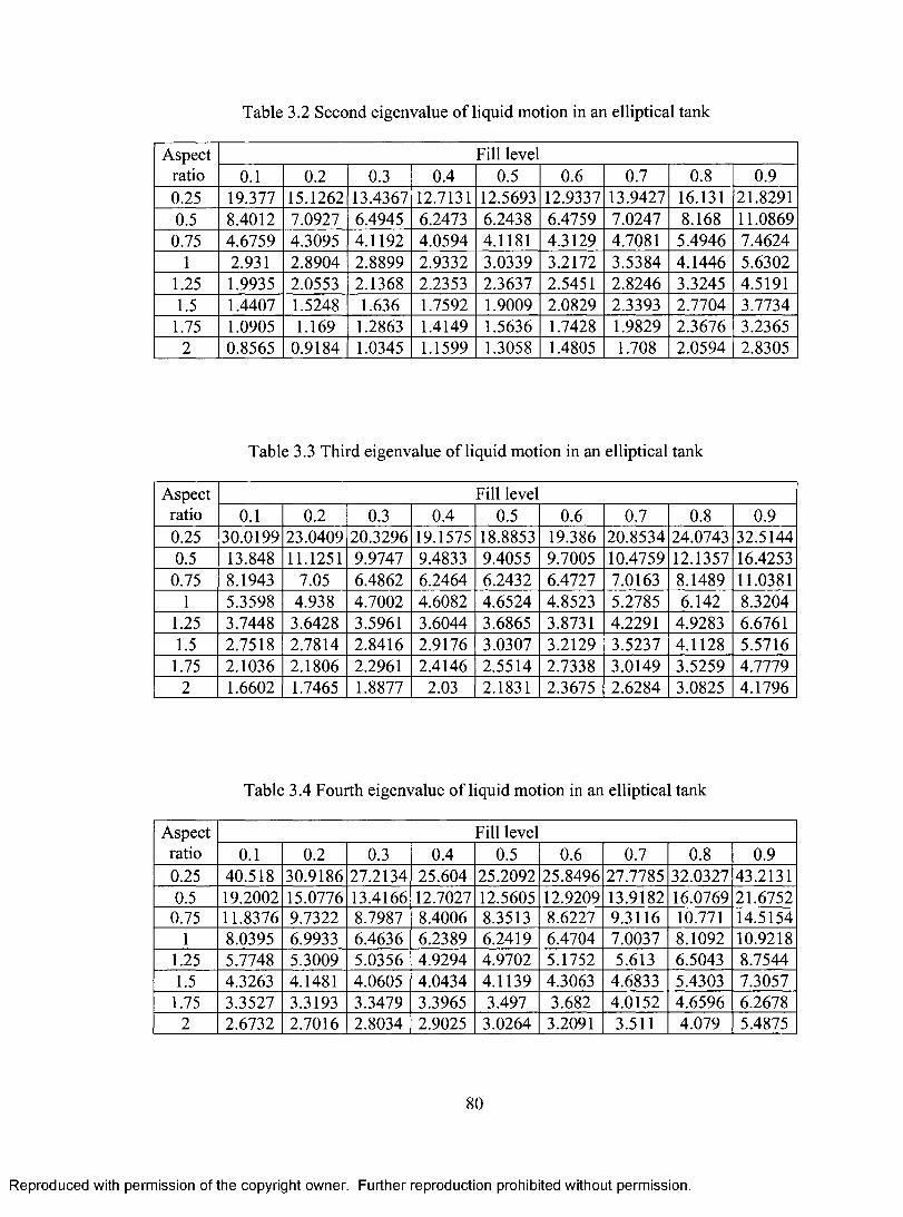
Table 3.2 Second eigenvalue of liquid motion in an elliptical tank
Aspect ratio
Fill level 0.1 0.2 0.3 0.4 0.5 0.6 0.7 0.8 0.9
0.25 19.377 15.1262 13.4367 12.7131 12.5693 12.9337 13.9427 16.131 21.8291 0.5 8.4012 7.0927 6.4945 6.2473 6.2438 6.4759 7.0247 8.168 11.0869
0.75 4.6759 4.3095 4.1192 4.0594 4.1181 4.3129 4.7081 5.4946 7.4624 1 2.931 2.8904 2.8899 2.9332 3.0339 3.2172 3.5384 4.1446 5.6302
1.25 1.9935 2.0553 2.1368 2.2353 2.3637 2.5451 2.8246 3.3245 4.5191 1.5 1.4407 1.5248 1.636 1.7592 1.9009 2.0829 2.3393 2.7704 3.7734
1.75 1.0905 1.169 1.2863 1.4149 1.5636 1.7428 1.9829 2.3676 3.2365 2 0.8565 0.9184 1.0345 1.1599 1.3058 1.4805 1.708 2.0594 2.8305
Table 3.3 Third eigenvalue of liquid motion in an elliptical tank
Aspect ratio
Fill level 0.1 0.2 0.3 0.4 0.5 0.6 0.7 0.8 0.9
0.25 30.0199 23.0409 20.3296 19.1575 18.8853 19.386 20.8534 24.0743 32.5144 0.5 13.848 11.1251 9.9747 9.4833 9.4055 9.7005 10.4759 12.1357 16.4253
0.75 8.1943 7.05 6.4862 6.2464 6.2432 6.4727 7.0163 8.1489 11.0381 1 5.3598 4.938 4.7002 4.6082 4.6524 4.8523 5.2785 6.142 8.3204
1.25 3.7448 3.6428 3.5961 3.6044 3.6865 3.8731 4.2291 4.9283 6.6761 1.5 2.7518 2.7814 2.8416 2.9176 3.0307 3.2129 3.5237 4.1128 5.5716
1.75 2.1036 2.1806 2.2961 2.4146 2.5514 2.7338 3.0149 3.5259 4.7779 2 1.6602 1.7465 1.8877 2.03 2.1831 2.3675 2.6284 3.0825 4.1796
Table 3.4 Fourth eigenvalue of liquid motion in an elliptical tank
Aspect ratio
Fill level 0.1 0.2 0.3 0.4 0.5 0.6 0.7 0.8 0.9
0.25 40.518 30.9186 27.2134 25.604 25.2092 25.8496 27.7785 32.0327 43.2131 0.5 19.2002 15.0776 13.4166 12.7027 12.5605 12.9209 13.9182 16.0769 21.6752
0.75 11.8376 9.7322 8.7987 8.4006 8.3513 8.6227 9.3116 10.771 14.5154 1 8.0395 6.9933 6.4636 6.2389 6.2419 6.4704 7.0037 8.1092 10.9218
1.25 5.7748 5.3009 5.0356 4.9294 4.9702 5.1752 5.613 6.5043 8.7544 1.5 4.3263 4.1481 4.0605 4.0434 4.1139 4.3063 4.6833 5.4303 7.3057
1.75 3.3527 3.3193 3.3479 3.3965 3.497 3.682 4.0152 4.6596 6.2678 2 2.6732 2.7016 2.8034 2.9025 3.0264 3.2091 3.511 4.079 5.4875
80
Reproduced with permission of the copyright owner. Further reproduction prohibited without permission.
Table 3.2 Second eigenvalue o f liquid motion in an elliptical tank
Aspectratio
Fill level0.1 0.2 0.3 0.4 0.5 0.6 0.7 0.8 0.9
0.25 19.377 15.1262 13.4367 12.7131 12.5693 12.9337 13.9427 16.131 21.82910.5 8.4012 7.0927 6.4945 6.2473 6.2438 6.4759 7.0247 8.168 11.0869
0.75 4.6759 4.3095 4.1192 4.0594 4.1181 4.3129 4.7081 5.4946 7.46241 2.931 2.8904 2.8899 2.9332 3.0339 3.2172 3.5384 4.1446 5.6302
1.25 1.9935 2.0553 2.1368 2.2353 2.3637 2.5451 2.8246 3.3245 4.51911.5 1.4407 1.5248 1.636 1.7592 1.9009 2.0829 2.3393 2.7704 3.7734
1.75 1.0905 1.169 1.2863 1.4149 1.5636 1.7428 1.9829 2.3676 3.23652 0.8565 0.9184 1.0345 1.1599 1.3058 1.4805 1.708 2.0594 2.8305
Table 3.3 Third eigenvalue o f liquid motion in an elliptical tank
Aspectratio
Fill level0.1 0.2 0.3 0.4 0.5 0.6 0.7 0.8 0.9
0.25 30.0199 23.0409 20.3296 19.1575 18.8853 19.386 20.8534 24.0743 32.51440.5 13.848 11.1251 9.9747 9.4833 9.4055 9.7005 10.4759 12.1357 16.4253
0.75 8.1943 7.05 6.4862 6.2464 6.2432 6.4727 7.0163 8.1489 11.03811 5.3598 4.938 4.7002 4.6082 4.6524 4.8523 5.2785 6.142 8.3204
1.25 3.7448 3.6428 3.5961 3.6044 3.6865 3.8731 4.2291 4.9283 6.67611.5 2.7518 2.7814 2.8416 2.9176 3.0307 3.2129 3.5237 4.1128 5.5716
1.75 2.1036 2.1806 2.2961 2.4146 2.5514 2.7338 3.0149 3.5259 4.77792 1.6602 1.7465 1.8877 2.03 2.1831 2.3675 2.6284 3.0825 4.1796
Table 3.4 Fourth eigenvalue of liquid motion in an elliptical tank
Aspectratio
Fill level0.1 0.2 0.3 0.4 0.5 0.6 0.7 0.8 0.9
0.25 40.518 30.9186 27.2134 25.604 25.2092 25.8496 27.7785 32.0327 43.21310.5 19.2002 15.0776 13.4166 12.7027 12.5605 12.9209 13.9182 16.0769 21.6752
0.75 11.8376 9.7322 8.7987 8.4006 8.3513 8.6227 9.3116 10.771 14.51541 8.0395 6.9933 6.4636 6.2389 6.2419 6.4704 7.0037 8.1092 10.9218
1.25 5.7748 5.3009 5.0356 4.9294 4.9702 5.1752 5.613 6.5043 8.75441.5 4.3263 4.1481 4.0605 4.0434 4.1139 4.3063 4.6833 5.4303 7.3057
1.75 3.3527 3.3193 3.3479 3.3965 3.497 3.682 4.0152 4.6596 6.26782 2.6732 2.7016 2.8034 2.9025 3.0264 3.2091 3.511 4.079 5.4875
Reproduced with permission of the copyright owner. Further reproduction prohibited without permission.
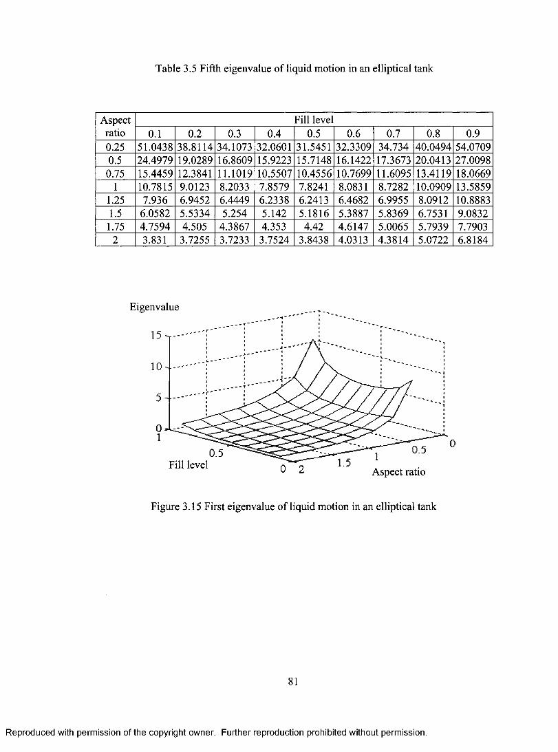
Table 3.5 Fifth eigenvalue of liquid motion in an elliptical tank
Aspect ratio
Fill level 0.1 0.2 0.3 0.4 0.5 0.6 0.7 0.8 0.9
0.25 51.0438 38.8114 34.1073 32.0601 31.5451 32.3309 34.734 40.0494 54.0709 0.5 24.4979 19.0289 16.8609 15.9223 15.7148 16.1422 17.3673 20.0413 27.0098 0.75 15.4459 12.3841 11.1019 10.5507 10.4556 10.7699 11.6095 13.4119 18.0669
1 10.7815 9.0123 8.2033 7.8579 7.8241 8.0831 8.7282 10.0909 13.5859 1.25 7.936 6.9452 6.4449 6.2338 6.2413 6.4682 6.9955 8.0912 10.8883 1.5 6.0582 5.5334 5.254 5.142 5.1816 5.3887 5.8369 6.7531 9.0832 1.75 4.7594 4.505 4.3867 4.353 4.42 4.6147 5.0065 5.7939 7.7903
2 3.831 3.7255 3.7233 3.7524 3.8438 4.0313 4.3814 5.0722 6.8184
Eigenvalue
15 ''''-
10 ''''
5 - 111111 140 a-,,A101010 1°41.14 01
M I •_ I I I I I I I I 1" -_,dollow' WO -41% 101.1 44%••••4-- -41,1-4 01*--"
0.5 Fill level 1.5
1
Aspect ratio
0.5
Figure 3.15 First eigenvalue of liquid motion in an elliptical tank
81
Reproduced with permission of the copyright owner. Further reproduction prohibited without permission.
Table 3.5 Fifth eigenvalue of liquid motion in an elliptical tank
Aspectratio
Fill level0.1 0.2 0.3 0.4 0.5 0.6 0.7 0.8 0.9
0.25 51.0438 38.8114 34.1073 32.0601 31.5451 32.3309 34.734 40.0494 54.07090.5 24.4979 19.0289 16.8609 15.9223 15.7148 16.1422 17.3673 20.0413 27.0098
0.75 15.4459 12.3841 11.1019 10.5507 10.4556 10.7699 11.6095 13.4119 18.06691 10.7815 9.0123 8.2033 7.8579 7.8241 8.0831 8.7282 10.0909 13.5859
1.25 7.936 6.9452 6.4449 6.2338 6.2413 6.4682 6.9955 8.0912 10.88831.5 6.0582 5.5334 5.254 5.142 5.1816 5.3887 5.8369 6.7531 9.0832
1.75 4.7594 4.505 4.3867 4.353 4.42 4.6147 5.0065 5.7939 7.79032 3.831 3.7255 3.7233 3.7524 3.8438 4.0313 4.3814 5.0722 6.8184
Eigenvalue
0.50.5Fill level
Aspect ratio
Figure 3.15 First eigenvalue o f liquid motion in an elliptical tank
Reproduced with permission of the copyright owner. Further reproduction prohibited without permission.
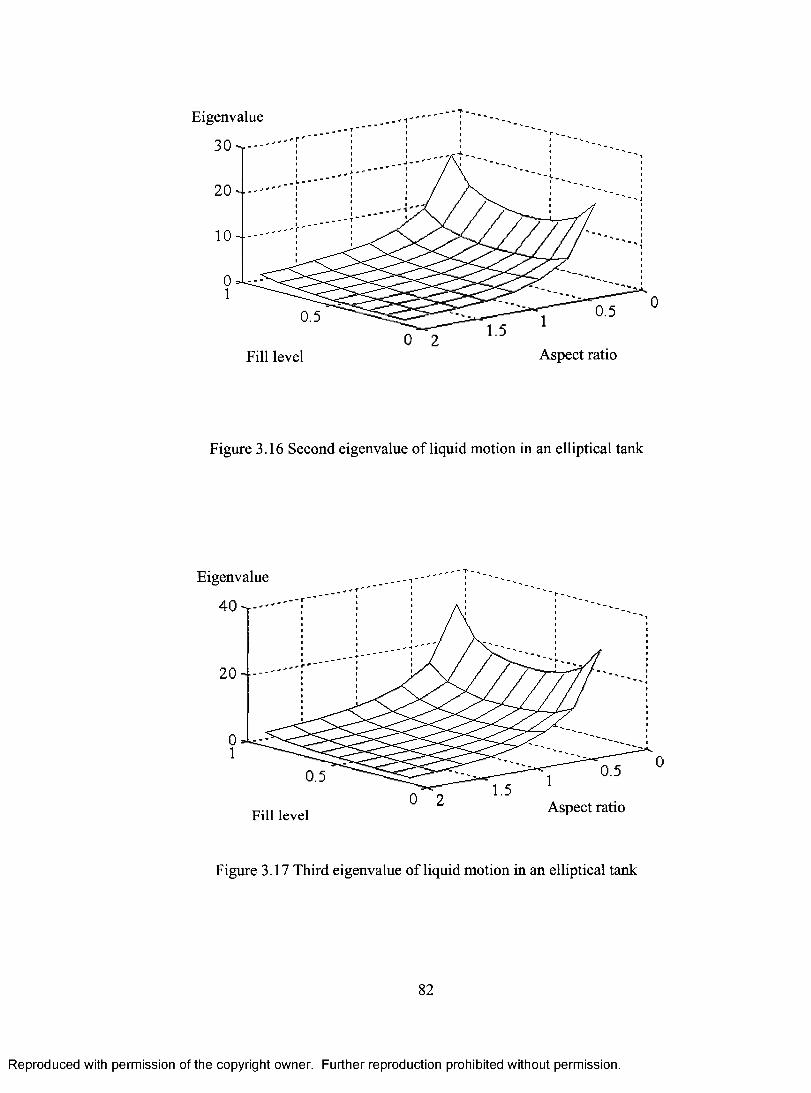
Eigenvalue
30 ''''''
Fill level Aspect ratio
Figure 3.16 Second eigenvalue of liquid motion in an elliptical tank
Eigenvalue ''''
#1110*Iri i
I I IA I *b Ill I I P -4 I lit. I I I I I I • -4 I PA P O
'41 11111F111.1W-
40 ---
20
0.5
Fill level
1.5 1 0.5
Aspect ratio
Figure 3.17 Third eigenvalue of liquid motion in an elliptical tank
82
Reproduced with permission of the copyright owner. Further reproduction prohibited without permission.
Eigenvalue
30 >---
20
0.50.5
Aspect ratioFill level
Figure 3.16 Second eigenvalue o f liquid motion in an elliptical tank
Eigenvalue
4 0 ~ r-"
0.50.5
Aspect ratioFill level
Figure 3.17 Third eigenvalue of liquid motion in an elliptical tank
82
Reproduced with permission of the copyright owner. Further reproduction prohibited without permission.
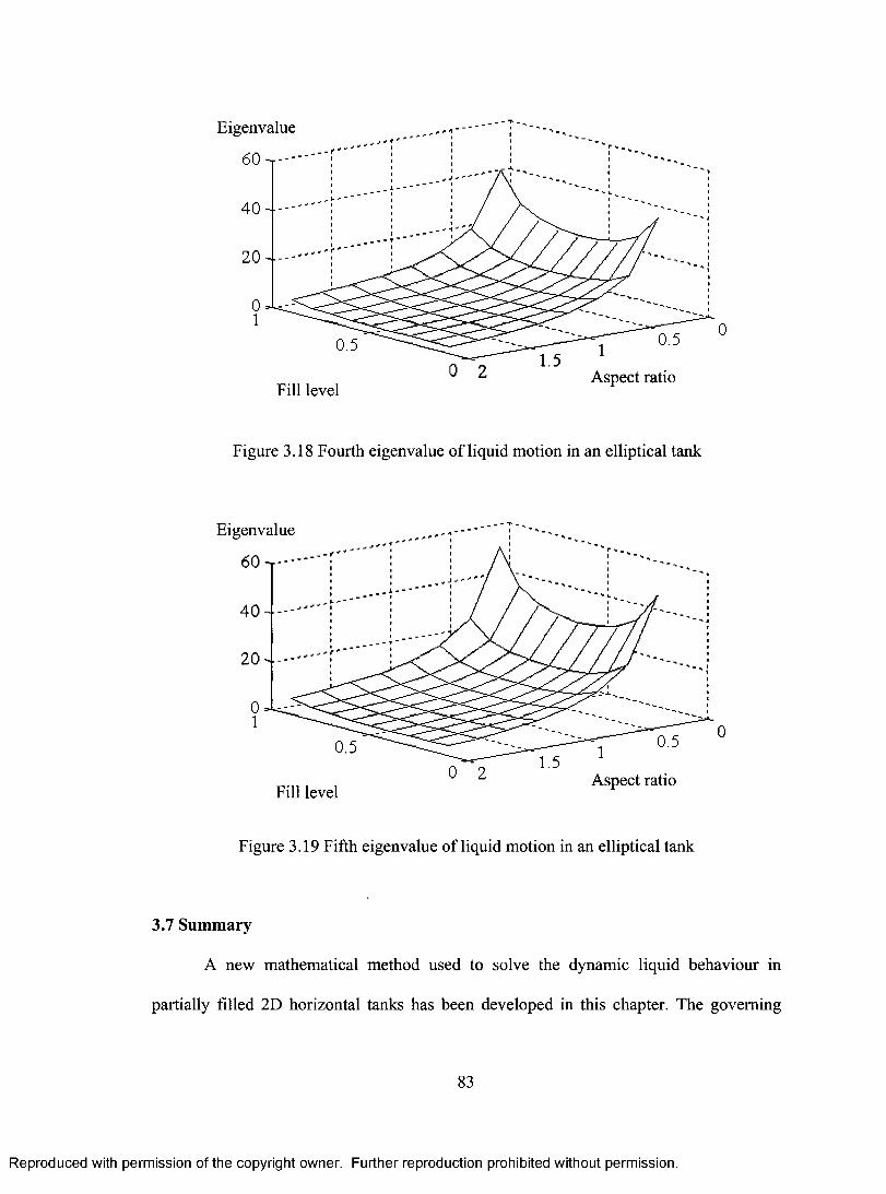
0.5
Fill level
1.5 1Aspect ratio
0.5
Figure 3.18 Fourth eigenvalue of liquid motion in an elliptical tank
Eigenvalue
60 --------r.
—
Fill level Aspect ratio
Figure 3.19 Fifth eigenvalue of liquid motion in an elliptical tank
3.7 Summary
A new mathematical method used to solve the dynamic liquid behaviour in
partially filled 2D horizontal tanks has been developed in this chapter. The governing
83
Reproduced with permission of the copyright owner. Further reproduction prohibited without permission.
Eigenvalue
6 0 -r —
0.50.5
Aspect ratioFill level
Figure 3.18 Fourth eigenvalue of liquid motion in an elliptical tank
Eigenvalue
60 t —
0.50.5
Aspect ratioFill level
0
Figure 3.19 Fifth eigenvalue o f liquid motion in an elliptical tank
3.7 Summary
A new mathematical method used to solve the dynamic liquid behaviour in
partially filled 2D horizontal tanks has been developed in this chapter. The governing
83
Reproduced with permission of the copyright owner. Further reproduction prohibited without permission.
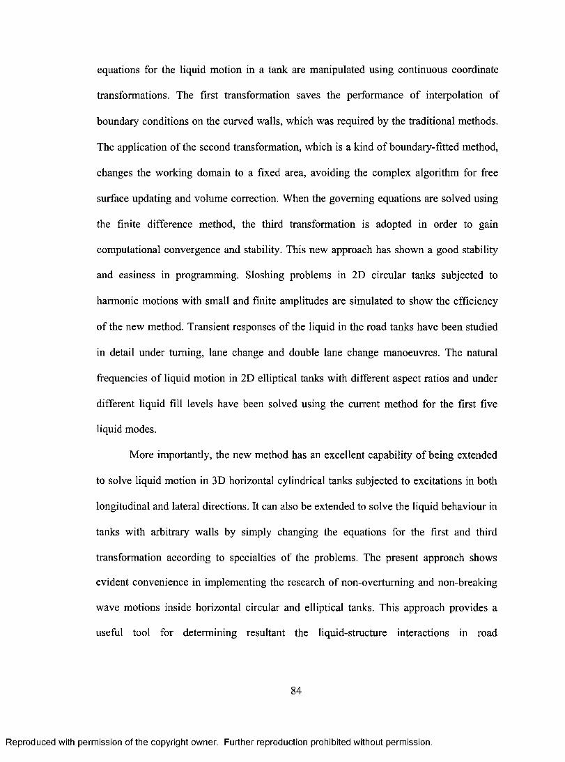
equations for the liquid motion in a tank are manipulated using continuous coordinate
transformations. The first transformation saves the performance of interpolation of
boundary conditions on the curved walls, which was required by the traditional methods.
The application of the second transformation, which is a kind of boundary-fitted method,
changes the working domain to a fixed area, avoiding the complex algorithm for free
surface updating and volume correction. When the governing equations are solved using
the finite difference method, the third transformation is adopted in order to gain
computational convergence and stability. This new approach has shown a good stability
and easiness in programming. Sloshing problems in 2D circular tanks subjected to
harmonic motions with small and finite amplitudes are simulated to show the efficiency
of the new method. Transient responses of the liquid in the road tanks have been studied
in detail under turning, lane change and double lane change manoeuvres. The natural
frequencies of liquid motion in 2D elliptical tanks with different aspect ratios and under
different liquid fill levels have been solved using the current method for the first five
liquid modes.
More importantly, the new method has an excellent capability of being extended
to solve liquid motion in 3D horizontal cylindrical tanks subjected to excitations in both
longitudinal and lateral directions. It can also be extended to solve the liquid behaviour in
tanks with arbitrary walls by simply changing the equations for the first and third
transformation according to specialties of the problems. The present approach shows
evident convenience in implementing the research of non-overturning and non-breaking
wave motions inside horizontal circular and elliptical tanks. This approach provides a
useful tool for determining resultant the liquid-structure interactions in road
84
Reproduced with permission of the copyright owner. Further reproduction prohibited without permission.
equations for the liquid motion in a tank are manipulated using continuous coordinate
transformations. The first transformation saves the performance o f interpolation of
boundary conditions on the curved walls, which was required by the traditional methods.
The application o f the second transformation, which is a kind of boundary-fitted method,
changes the working domain to a fixed area, avoiding the complex algorithm for free
surface updating and volume correction. When the governing equations are solved using
the finite difference method, the third transformation is adopted in order to gain
computational convergence and stability. This new approach has shown a good stability
and easiness in programming. Sloshing problems in 2D circular tanks subjected to
harmonic motions with small and finite amplitudes are simulated to show the efficiency
o f the new method. Transient responses o f the liquid in the road tanks have been studied
in detail under turning, lane change and double lane change manoeuvres. The natural
frequencies o f liquid motion in 2D elliptical tanks with different aspect ratios and under
different liquid fill levels have been solved using the current method for the first five
liquid modes.
More importantly, the new method has an excellent capability o f being extended
to solve liquid motion in 3D horizontal cylindrical tanks subjected to excitations in both
longitudinal and lateral directions. It can also be extended to solve the liquid behaviour in
tanks with arbitrary walls by simply changing the equations for the first and third
transformation according to specialties o f the problems. The present approach shows
evident convenience in implementing the research o f non-overturning and non-breaking
wave motions inside horizontal circular and elliptical tanks. This approach provides a
useful tool for determining resultant the liquid-structure interactions in road
84
Reproduced with permission of the copyright owner. Further reproduction prohibited without permission.
transportation and other relevant engineering fields. The development of the method for
liquid motion in 3D cylindrical tanks and the application of the new method in studying
3D liquid dynamics will be conducted in the following chapter.
85
Reproduced with permission of the copyright owner. Further reproduction prohibited without permission.
transportation and other relevant engineering fields. The development o f the method for
liquid motion in 3D cylindrical tanks and the application of the new method in studying
3D liquid dynamics will be conducted in the following chapter.
85
Reproduced with permission of the copyright owner. Further reproduction prohibited without permission.

CHAPTER 4 LIQUID MOTION IN 3D HORIZONTAL
CYLINDRICAL TANKS
4.1 Introduction
In the current literature, 2D sloshing models have been combined with 3D vehicle
models in almost all studies on vehicle dynamics for liquid cargo vehicles. For the lateral
liquid models, the liquid motion is described only in the transverse direction with the
assumption that the liquid in all cross sections of the cylindrical tank behaves identically
from the head to the end of the tank. This may be reasonable if the tank only suffers the
excitation in the transverse direction. However, for tanks used in road vehicles, this
cannot be true. In the turning, lane change and double lane change operations, the mass
centre of the tank is subjected to the translational and rotational accelerations in all six
directions. Even when the tank is considered to be turned along a perfect circular curve
with a constant forward speed, where the mass centre of the tank is only subjected to a
constant centrifugal acceleration, the liquid particles at different positions in the tank can
become subject to different lateral and longitudinal accelerations. Therefore, even for this
case, the above assumption cannot show the real motion of the liquid. For turning along
arbitrary trajectories and the lane change and double lane change, the mass centre of the
tank is subjected to both tangential acceleration and centrifugal acceleration. The motion
of the liquid particles should then be determined according to these time varying
accelerations. The assumption that the liquid has the same behaviour at different cross
sections neglects the longitudinal effect exerted on the liquid. Also, the application of the
same constant lateral acceleration on all cross sections cannot show the lateral
86
Reproduced with permission of the copyright owner. Further reproduction prohibited without permission.
CHAPTER 4 LIQUID MOTION IN 3D HORIZONTAL
CYLINDRICAL TANKS
4.1 Introduction
In the current literature, 2D sloshing models have been combined with 3D vehicle
models in almost all studies on vehicle dynamics for liquid cargo vehicles. For the lateral
liquid models, the liquid motion is described only in the transverse direction with the
assumption that the liquid in all cross sections o f the cylindrical tank behaves identically
from the head to the end of the tank. This may be reasonable if the tank only suffers the
excitation in the transverse direction. However, for tanks used in road vehicles, this
cannot be true. In the turning, lane change and double lane change operations, the mass
centre o f the tank is subjected to the translational and rotational accelerations in all six
directions. Even when the tank is considered to be turned along a perfect circular curve
with a constant forward speed, where the mass centre o f the tank is only subjected to a
constant centrifugal acceleration, the liquid particles at different positions in the tank can
become subject to different lateral and longitudinal accelerations. Therefore, even for this
case, the above assumption cannot show the real motion of the liquid. For turning along
arbitrary trajectories and the lane change and double lane change, the mass centre o f the
tank is subjected to both tangential acceleration and centrifugal acceleration. The motion
of the liquid particles should then be determined according to these time varying
accelerations. The assumption that the liquid has the same behaviour at different cross
sections neglects the longitudinal effect exerted on the liquid. Also, the application of the
same constant lateral acceleration on all cross sections cannot show the lateral
86
Reproduced with permission of the copyright owner. Further reproduction prohibited without permission.
acceleration differences among the liquid particles. For some situations, turning, lane
change and double lane change operations are often performed along with braking or
accelerating. For these cases, the influence of the tangential acceleration is much more
significant. For all of the above situations, the forces and moments obtained from the
liquid motion model considered only in the lateral direction are undoubtedly unable to
accurately reflect the true liquid action on the tank and the vehicle. When using the
resultant tank motion as the input to calculate the liquid motion for the next time step, the
simulation can hardly be reliable. The simulation results will, in the long run, derivate
from the true response.
During ideal straight line driving, the tank is subjected to translational
accelerations in the longitudinal and vertical directions, as well as rotational acceleration
in the pitch plane. In this case, the longitudinal liquid model is needed. It can be found in
the current literature that rectangular tanks, which are not common in road transportation
engineering, have been selected by researchers to study the vehicle dynamics in the
longitudinal direction, due to the difficulties of solving the governing equations in the 3D
space. For the rectangular tanks, existing algorithms for 2D liquid free surface problems,
such as the MAC method and VOF method, could be applied. However, because of the
existence of curved walls in the horizontal cylindrical tanks used by most liquid cargo
vehicles, the above schemes could hardly be extended to solve the liquid-vehicle system,
because the liquid motion in the longitudinal direction in cylindrical or elliptical tanks is
a 3D problem even for perfect straight line driving, braking and accelerating.
Obviously, the lack of an effective algorithm to solve the liquid sloshing problems
in horizontal cylindrical tanks in 3D space is the main reason that most studies on liquid
87
Reproduced with permission of the copyright owner. Further reproduction prohibited without permission.
acceleration differences among the liquid particles. For some situations, turning, lane
change and double lane change operations are often performed along with braking or
accelerating. For these cases, the influence of the tangential acceleration is much more
significant. For all o f the above situations, the forces and moments obtained from the
liquid motion model considered only in the lateral direction are undoubtedly unable to
accurately reflect the true liquid action on the tank and the vehicle. When using the
resultant tank motion as the input to calculate the liquid motion for the next time step, the
simulation can hardly be reliable. The simulation results will, in the long run, derivate
from the true response.
During ideal straight line driving, the tank is subjected to translational
accelerations in the longitudinal and vertical directions, as well as rotational acceleration
in the pitch plane. In this case, the longitudinal liquid model is needed. It can be found in
the current literature that rectangular tanks, which are not common in road transportation
engineering, have been selected by researchers to study the vehicle dynamics in the
longitudinal direction, due to the difficulties of solving the governing equations in the 3D
space. For the rectangular tanks, existing algorithms for 2D liquid free surface problems,
such as the MAC method and VOF method, could be applied. However, because o f the
existence of curved walls in the horizontal cylindrical tanks used by most liquid cargo
vehicles, the above schemes could hardly be extended to solve the liquid-vehicle system,
because the liquid motion in the longitudinal direction in cylindrical or elliptical tanks is
a 3D problem even for perfect straight line driving, braking and accelerating.
Obviously, the lack of an effective algorithm to solve the liquid sloshing problems
in horizontal cylindrical tanks in 3D space is the main reason that most studies on liquid
87
Reproduced with permission of the copyright owner. Further reproduction prohibited without permission.
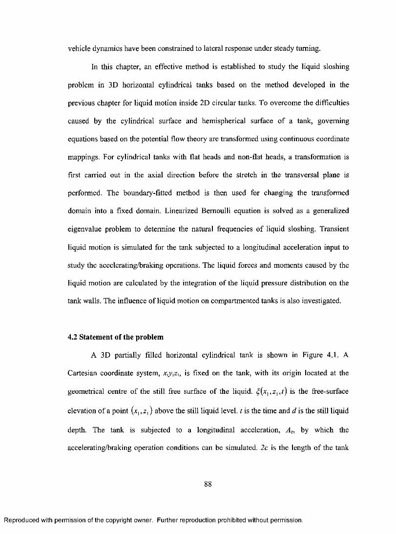
vehicle dynamics have been constrained to lateral response under steady turning.
In this chapter, an effective method is established to study the liquid sloshing
problem in 3D horizontal cylindrical tanks based on the method developed in the
previous chapter for liquid motion inside 2D circular tanks. To overcome the difficulties
caused by the cylindrical surface and hemispherical surface of a tank, governing
equations based on the potential flow theory are transformed using continuous coordinate
mappings. For cylindrical tanks with flat heads and non-flat heads, a transformation is
first carried out in the axial direction before the stretch in the transversal plane is
performed. The boundary-fitted method is then used for changing the transformed
domain into a fixed domain. Linearized Bernoulli equation is solved as a generalized
eigenvalue problem to determine the natural frequencies of liquid sloshing. Transient
liquid motion is simulated for the tank subjected to a longitudinal acceleration input to
study the accelerating/braking operations. The liquid forces and moments caused by the
liquid motion are calculated by the integration of the liquid pressure distribution on the
tank walls. The influence of liquid motion on compartmented tanks is also investigated.
4.2 Statement of the problem
A 3D partially filled horizontal cylindrical tank is shown in Figure 4.1. A
Cartesian coordinate system, xiyizi, is fixed on the tank, with its origin located at the
geometrical centre of the still free surface of the liquid. (x1,z, , t) is the free-surface
elevation of a point (x1,z,) above the still liquid level. t is the time and d is the still liquid
depth. The tank is subjected to a longitudinal acceleration, Az, by which the
accelerating/braking operation conditions can be simulated. 2c is the length of the tank
88
Reproduced with permission of the copyright owner. Further reproduction prohibited without permission.
vehicle dynamics have been constrained to lateral response under steady turning.
In this chapter, an effective method is established to study the liquid sloshing
problem in 3D horizontal cylindrical tanks based on the method developed in the
previous chapter for liquid motion inside 2D circular tanks. To overcome the difficulties
caused by the cylindrical surface and hemispherical surface o f a tank, governing
equations based on the potential flow theory are transformed using continuous coordinate
mappings. For cylindrical tanks with flat heads and non-flat heads, a transformation is
first carried out in the axial direction before the stretch in the transversal plane is
performed. The boundary-fitted method is then used for changing the transformed
domain into a fixed domain. Linearized Bernoulli equation is solved as a generalized
eigenvalue problem to determine the natural frequencies o f liquid sloshing. Transient
liquid motion is simulated for the tank subjected to a longitudinal acceleration input to
study the accelerating/braking operations. The liquid forces and moments caused by the
liquid motion are calculated by the integration o f the liquid pressure distribution on the
tank walls. The influence o f liquid motion on compartmented tanks is also investigated.
4.2 Statement of the problem
A 3D partially filled horizontal cylindrical tank is shown in Figure 4.1. A
Cartesian coordinate system, is fixed on the tank, with its origin located at the
geometrical centre of the still free surface of the liquid. %{xx, z x,t) is the free-surface
elevation o f a point (x, ,z ,) above the still liquid level, t is the time and d is the still liquid
depth. The tank is subjected to a longitudinal acceleration, Az, by which the
accelerating/braking operation conditions can be simulated. 2 c is the length of the tank
88
Reproduced with permission of the copyright owner. Further reproduction prohibited without permission.
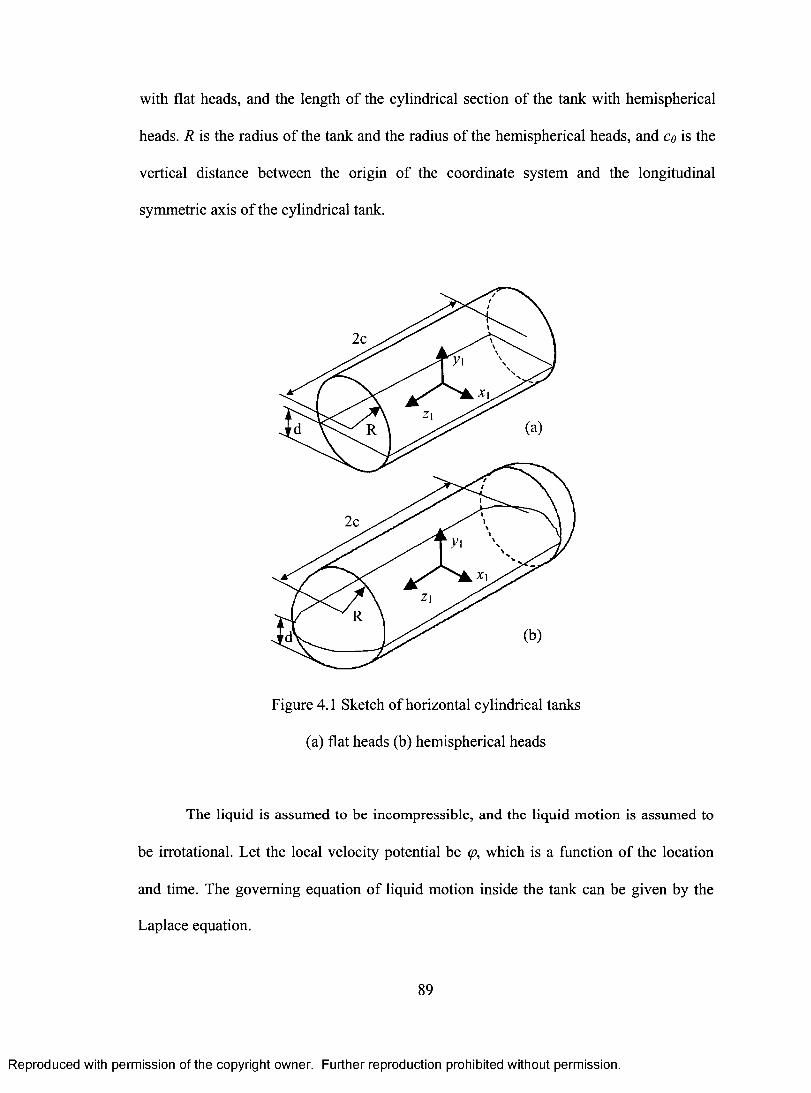
with flat heads, and the length of the cylindrical section of the tank with hemispherical
heads. R is the radius of the tank and the radius of the hemispherical heads, and co is the
vertical distance between the origin of the coordinate system and the longitudinal
symmetric axis of the cylindrical tank.
Figure 4.1 Sketch of horizontal cylindrical tanks
(a) flat heads (b) hemispherical heads
The liquid is assumed to be incompressible, and the liquid motion is assumed to
be irrotational. Let the local velocity potential be q,, which is a function of the location
and time. The governing equation of liquid motion inside the tank can be given by the
Laplace equation.
89
Reproduced with permission of the copyright owner. Further reproduction prohibited without permission.
with flat heads, and the length of the cylindrical section of the tank with hemispherical
heads. R is the radius o f the tank and the radius o f the hemispherical heads, and co is the
vertical distance between the origin of the coordinate system and the longitudinal
symmetric axis o f the cylindrical tank.
Figure 4.1 Sketch of horizontal cylindrical tanks
(a) flat heads (b) hemispherical heads
The liquid is assumed to be incompressible, and the liquid m otion is assumed to
be irrotational. Let the local velocity potential be (p, which is a function o f the location
and time. The governing equation o f liquid motion inside the tank can be given by the
Laplace equation.
89
Reproduced with permission of the copyright owner. Further reproduction prohibited without permission.
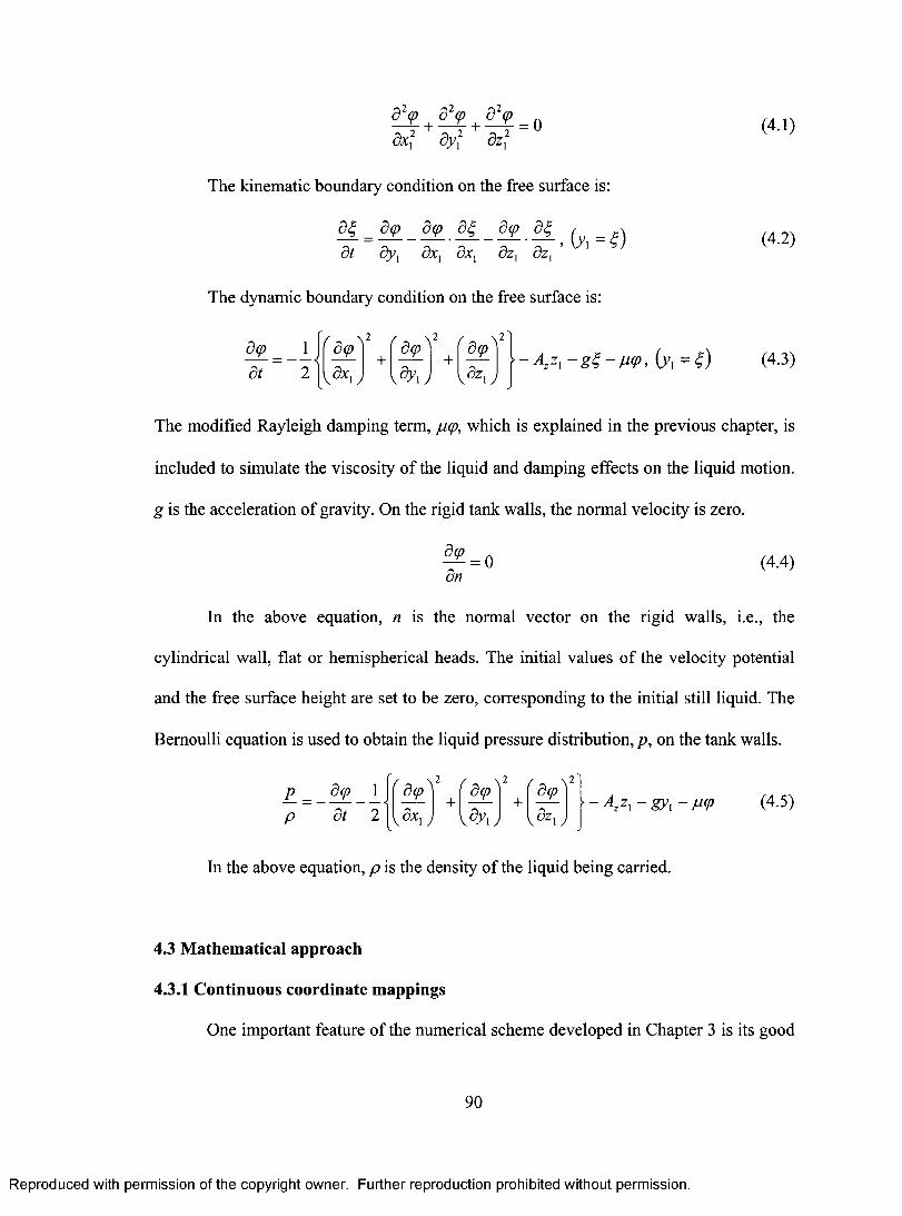
a2 v ± a2co ± a2 v = 0
ax; ay, az
The kinematic boundary condition on the free surface is:
a _4 4 ta 4 a , (yi _ ) at ay, ax, ax, az, az,
The dynamic boundary condition on the free surface is:
ac — 1 __ at 2 ax,,
ao \ 2 ( \2 aci + +
\aY1 ) Paz, }( aq' 2 — Azz, —g — MD, (y1 = 6
(4.1)
(4.2)
(4.3)
The modified Rayleigh damping term, ,ugo, which is explained in the previous chapter, is
included to simulate the viscosity of the liquid and damping effects on the liquid motion.
g is the acceleration of gravity. On the rigid tank walls, the normal velocity is zero.
aq' =o an (4.4)
In the above equation, n is the normal vector on the rigid walls, i.e., the
cylindrical wall, flat or hemispherical heads. The initial values of the velocity potential
and the free surface height are set to be zero, corresponding to the initial still liquid. The
Bernoulli equation is used to obtain the liquid pressure distribution, p, on the tank walls.
P 4 -\ 2 aco
P at 2 ax 1 \
( 2 / \ 2} aco aq, — Az z l — gyp — P+ +
\.. aYi \, ) aZ1 O/
)
In the above equation, p is the density of the liquid being carried.
(4.5)
4.3 Mathematical approach
4.3.1 Continuous coordinate mappings
One important feature of the numerical scheme developed in Chapter 3 is its good
90
Reproduced with permission of the copyright owner. Further reproduction prohibited without permission.
d 2<P d 2(p d 2<pdxf dyx dzx
The kinematic boundary condition on the free surface is:
dt; _ dcp dcp dt; dcp dt; , _ \dt dyx dxi dxx dzx dzx ’
The dynamic boundary condition on the free surface is:
(4.1)
(4.2)
dcpdt
/ d^ 2
\ dx\ j
r dkp^2
V ^i j+
' d(p 2
v& i j~ A Z\ - g £ - w > U =4) (4.3)
The modified Rayleigh damping term, /icp, which is explained in the previous chapter, is
included to simulate the viscosity o f the liquid and damping effects on the liquid motion.
g is the acceleration o f gravity. On the rigid tank walls, the normal velocity is zero.
^ = 0dn
(4.4)
In the above equation, n is the normal vector on the rigid walls, i.e., the
cylindrical wall, flat or hemispherical heads. The initial values o f the velocity potential
and the free surface height are set to be zero, corresponding to the initial still liquid. The
Bernoulli equation is used to obtain the liquid pressure distribution, p, on the tank walls.
P_P
d(p 1 dt 2
' chp^ KdxXJ
dcp
\ p y \ j+
/ dcp 2
KdzXJ A z x - g y x-p(p (4.5)
In the above equation, p is the density of the liquid being carried.
4.3 Mathematical approach
4.3.1 Continuous coordinate mappings
One important feature of the numerical scheme developed in Chapter 3 is its good
90
Reproduced with permission of the copyright owner. Further reproduction prohibited without permission.
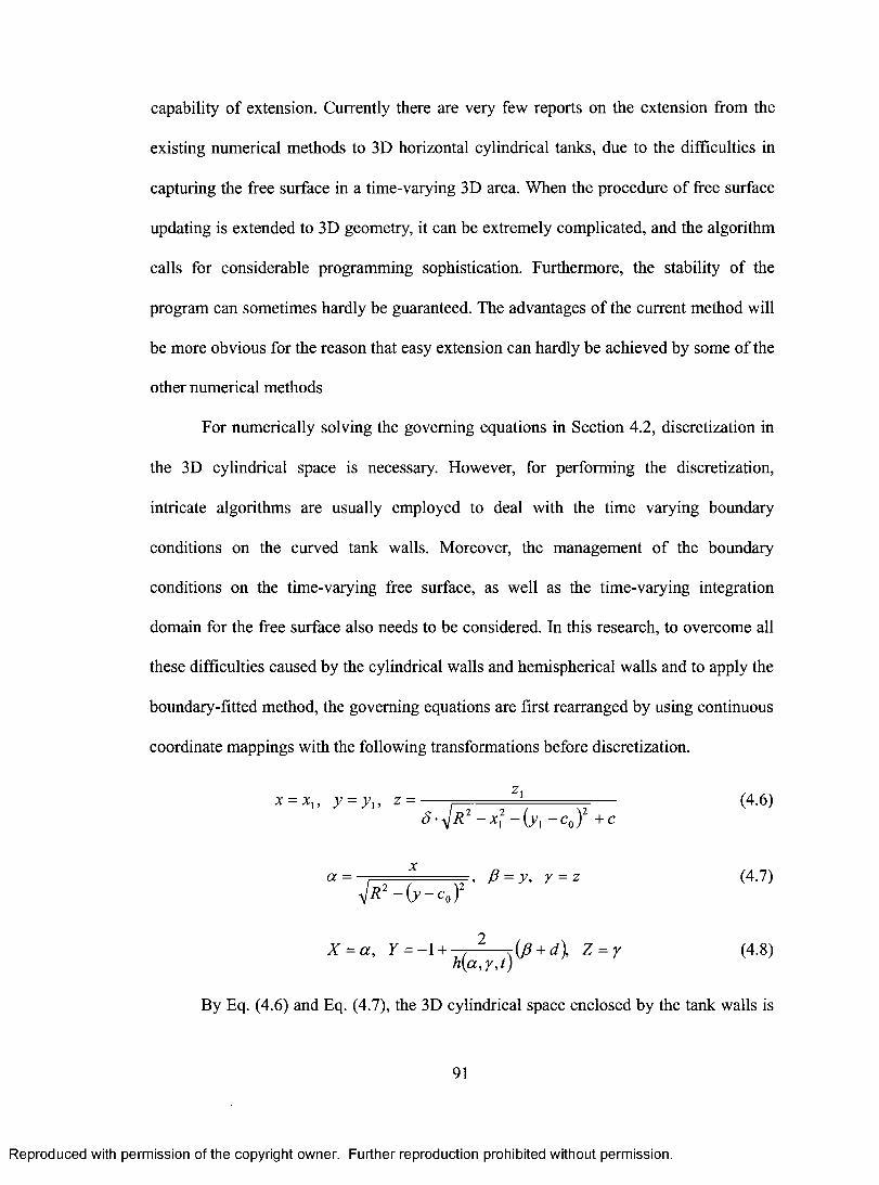
capability of extension. Currently there are very few reports on the extension from the
existing numerical methods to 3D horizontal cylindrical tanks, due to the difficulties in
capturing the free surface in a time-varying 3D area. When the procedure of free surface
updating is extended to 3D geometry, it can be extremely complicated, and the algorithm
calls for considerable programming sophistication. Furthermore, the stability of the
program can sometimes hardly be guaranteed. The advantages of the current method will
be more obvious for the reason that easy extension can hardly be achieved by some of the
other numerical methods
For numerically solving the governing equations in Section 4.2, discretization in
the 3D cylindrical space is necessary. However, for performing the discretization,
intricate algorithms are usually employed to deal with the time varying boundary
conditions on the curved tank walls. Moreover, the management of the boundary
conditions on the time-varying free surface, as well as the time-varying integration
domain for the free surface also needs to be considered. In this research, to overcome all
these difficulties caused by the cylindrical walls and hemispherical walls and to apply the
boundary-fitted method, the governing equations are first rearranged by using continuous
coordinate mappings with the following transformations before discretization.
x=xl , y=y1, z=
a= x
z1
8 . 11R 2 + xi2 + ( y1 + co )2 + c
AIR' — (y —c0 )2 '
(4.6)
fl = y, r = z (4.7)
, \ X=a 2 , Y=-1+ , , (fi+d), Z=7
10,y,t) (4.8)
By Eq. (4.6) and Eq. (4.7), the 3D cylindrical space enclosed by the tank walls is
91
Reproduced with permission of the copyright owner. Further reproduction prohibited without permission.
capability of extension. Currently there are very few reports on the extension from the
existing numerical methods to 3D horizontal cylindrical tanks, due to the difficulties in
capturing the free surface in a time-varying 3D area. When the procedure o f free surface
updating is extended to 3D geometry, it can be extremely complicated, and the algorithm
calls for considerable programming sophistication. Furthermore, the stability of the
program can sometimes hardly be guaranteed. The advantages o f the current method will
be more obvious for the reason that easy extension can hardly be achieved by some of the
other numerical methods
For numerically solving the governing equations in Section 4.2, discretization in
the 3D cylindrical space is necessary. However, for performing the discretization,
intricate algorithms are usually employed to deal with the time varying boundary
conditions on the curved tank walls. Moreover, the management o f the boundary
conditions on the time-varying free surface, as well as the time-varying integration
domain for the free surface also needs to be considered. In this research, to overcome all
these difficulties caused by the cylindrical walls and hemispherical walls and to apply the
boundary-fitted method, the governing equations are first rearranged by using continuous
coordinate mappings with the following transformations before discretization.
By Eq. (4.6) and Eq. (4.7), the 3D cylindrical space enclosed by the tank walls is
z.(4.6)
a = f3 = y, y = z (4.7)
(4.8)
91
Reproduced with permission of the copyright owner. Further reproduction prohibited without permission.
transformed from the xiy iz 1 coordinate system to an afly coordinate system, which results
in a working domain enclosed by a cubic box. By Eq.(4.6), a stretch is performed in the
axial direction, which is especially important for tanks with hemispherical heads. The
parameter 8is expressed as:
8= {oi flat heads
hemispherical heads (4.9)
By Eq.(4.7), a stretch is performed to avoid the complex algorithm for
interpolating the boundary conditions on curved tank walls. In order to avoid singularities,
the transformation is constrained by the following condition.
—1<ct 1, at /3=c0 ±R (4.10)
In Eq.(4.8), h is the total liquid height from the bottom to the transient free surface
in the afly coordinate system. Equation (4.8) reflects the boundary-fitted method, by
which the transformed liquid domain is further transformed into another cubic box in the
XYZ coordinate system, in which the vertical coordinate value, Y, changes with the
horizontal coordinate values, X and Z, and the time, t. Once again, it should be noted that,
for applying the boundary-fitted scheme, the above development is based on the
assumption that the liquid height is expressible as a single-value function of the location.
This implies that overturning waves and breaking waves will not occur during the motion
of the liquid tank, and the liquid will never hit the top of the tank or leave the bottom of
the tank in the case that sudden change of boundary conditions occurs. These
assumptions are commonly accepted by other researchers in this field. In fact, there still
exist no effective ways to numerically simulate these extreme cases by solving fluid
mechanics equations (Ibrahim et al, 2001).
92
Reproduced with permission of the copyright owner. Further reproduction prohibited without permission.
transformed from the x y xz x coordinate system to an afiy coordinate system, which results
in a working domain enclosed by a cubic box. By Eq.(4.6), a stretch is performed in the
axial direction, which is especially important for tanks with hemispherical heads. The
parameter S is expressed as:
By Eq.(4.7), a stretch is performed to avoid the complex algorithm for
interpolating the boundary conditions on curved tank walls. In order to avoid singularities,
the transformation is constrained by the following condition.
In Eq.(4.8), h is the total liquid height from the bottom to the transient free surface
in the afiy coordinate system. Equation (4.8) reflects the boundary-fitted method, by
which the transformed liquid domain is further transformed into another cubic box in the
XYZ coordinate system, in which the vertical coordinate value, Y, changes with the
horizontal coordinate values, X and Z, and the time, t. Once again, it should be noted that,
for applying the boundary-fitted scheme, the above development is based on the
assumption that the liquid height is expressible as a single-value function o f the location.
This implies that overturning waves and breaking waves will not occur during the motion
o f the liquid tank, and the liquid will never hit the top of the tank or leave the bottom of
the tank in the case that sudden change o f boundary conditions occurs. These
assumptions are commonly accepted by other researchers in this field. In fact, there still
exist no effective ways to numerically simulate these extreme cases by solving fluid
mechanics equations (Ibrahim et al, 2001).
f lat heads hemispherical heads
(4.9)
- 1 < « < 1 , at fi = c0 ± R (4.10)
92
Reproduced with permission of the copyright owner. Further reproduction prohibited without permission.
4.3.2 Formulae derivation
Applying Eqs. (4.6) and (4.7) to the governing equations (4.1)-(4.4) leads to the
following rearranged equations in the afiy coordinate system. The Laplace equation
becomes:
B• 82(4 +B• '32° +B• a2° +B 82° +B5• a20
• +B6•
a2A
Y' + B • B 8 • = 0 1 a ct 2 2 as2 3 ay2 4 a a ap may aaay 7 a a a,/
(4.11)
In the above equation, the coefficients are expressed by the metrics relating the
coordinate systems.
B 3
= (aa
+ (ace
+2 j 2
ax — ay
az " aa 801\
8X1 \ 8X 831
-N 2
, B2 =(—afi a y
7 az \ 2 \ 2 \ 2 2
aZ aZ ay a/3`+ + - • B 4 =
2(aa
ax ay, j az, j az ay ay
az ay az 'aa ay B
5 = 2—
ay, —az
' B6 = 2 ay, ay az
B 8
, B7 =
7 \2
7 aZ
\ 2
8X \ aYi
+2 az ' aa ale
ax, ax ay
raa 2 az a2a +
13Y .1 ax, axay
ay
az
The kinematic boundary condition on the free surface is transformed into:
=G• ° +G . a°at ' aa 816 3 ar
G =-8a +—aa ace) a77 ( ay az G _afi
ay ax aaax ) ay az ax, ) 2- ay
az 5a ari - ay aZ • 2. aZ 2
ax, ax aa az ` ax, az,
93
ari}ay
(4.12)
(4.13)
(4.14)
Reproduced with permission of the copyright owner. Further reproduction prohibited without permission.
4.3.2 Formulae derivation
Applying Eqs. (4.6) and (4.7) to the governing equations (4.1)-(4.4) leads to the
following rearranged equations in the afiy coordinate system. The Laplace equation
becomes:
da dp dy dadp dpdy dady d a dy(4.11)
In the above equation, the coefficients are expressed by the metrics relating the
coordinate systems.
5 ,= ( d a )2
+ 1 ^
1 a
2+ 2
dz ' rda da?, B2 =
' d p 'Vdx J Kfy ) ^ dx dy j
S3 =' d z V r d z vva*iy
B5 = 2
r d z ' 1
v ^ i j
dz dy dyx dz
v& iv
' dy_<l ydz
, B, = 2r d a d p '
dy dry+ 2
dzdxx
d a dp dx dy
2 ^ -da d y '
, Bn =
s 11 2 o dz + 2 ----
d 2adyx d z y 7 /
y d y ) dx | dxdy ’
Bq =' d z ' 2
ydX , ,+
r d z ' 2
\ f y \ j
dydz
(4.12)
The kinematic boundary condition on the free surface is transformed into:
drjdt
d(j)= G , 1- G1 1- G , -----
d(/> , ^ d<j>da dp dy
(4.13)
G, = — +da da I dr]dy dx \ da
dr} i dy dz dy v dz dxx j • ^ 2 =
dPdy ’
g 3 =( d y \Kdz ,
r d z ' dz d a djj dy dxx dx d a dz
' d z ' 2
y dxXJ+
r d z ' 1
ydzxJdr\dy
(4.14)
93
Reproduced with permission of the copyright owner. Further reproduction prohibited without permission.
The dynamic boundary condition on the free surface is transformed into:
•\ ao =_ 1 {E
, • ( -00 )2 +E 2.(a0 at 2 as afl)
E _ r aay + i ox ) r aa
)2 E = ay 2
E4 = 2 7 aa ap`
ay ay /
2 + E3 • ( '* 2 E a2° E E
6
a2d)Y" +E
} 7ay I
+ 4 aaap
• a2° + 5 apay
+ aaar
2 r IV \ —
, E3 .aY i
/ \ 2 r 2 2
az az j az ) + +aX 1 / \ ay, az,
az (as ay az (as ay` ,E =2— — —+ 2 — — —
5 ax aX az) ayi ay az j
az afl ay E6
ay az = 2 — [— —2±),E7 = - A zZi - gq — 44
i ay
(4.15)
paz ) ry
'
(4.16)
In the above equations, 0 is the corresponding potential and ri is the
corresponding liquid height in the afly coordinate system. The boundary conditions on
the walls parallel to the aj3, ay and fiyplanes are changed to the following equations.
ao 00 ao D
' • aa
+ D2
• ap
+ D3
• —ay
= 0
r a 0 , r a 0 , r3 •
ay 80
i • -- ri • -- ri • - =v
ap
a0 a0 a0 H1 •aa
— + H2 • ap — + I - I3 •ay
• — =0
D, = 8 •{ a
a
a aa / x1 + — 011 — c0 5 )1 D2 — • r ay , -.5 —co)
a D3 = 8 • { Oz x ± —oz (y, — co)+ az
• (z ± c)} • i-/ + (1— 8)• alax, ' ay, az, 1 az az
/1 = sa /2 =
94
_ ay az az ay,
(4.20)
(4.21)
Reproduced with permission of the copyright owner. Further reproduction prohibited without permission.
The dynamic boundary condition on the free surface is transformed into:
1 II 1 1 -
A F'i ■{d<)2
+ E 2 • f d<f>~)2
+ £ 3 •fdt 2 { d a ) I W ) [ d y )
+ £d 2(j)
+ E<d 2(j)
4 dad[3 5 dfidy+ e 6 -
d 2<j>+ £ 7
dady
(4.15)
E x =f da} 2
\ d x jr d a }
\ d y s, e 2 =
r dp} 2.^3 = ydXxj
+ f d z '* +V& 1 J
dydz
E4 =2 f da 8 0} dy dy
E6 = 2dzdyx
,E S = 2 — dx
dp dy dy dz
i V
d a dy dx dz
+ 2 d a dydyx Kdy dz
, £ 7 = - A tz x- g r \ - (4.16)
In the above equations, (j) is the corresponding potential and 77 is the
corresponding liquid height in the aPy coordinate system. The boundary conditions on
the walls parallel to the ap, ay and Py planes are changed to the following equations.
d</> d(/> d<t>D , h A !■ D, • — — 0
da dp J dy
/ r 3 £ + v M + / 3 . M = 0da dp dy
H, ■ - x - + / / , • — + H, • — = 0d<i>
da dp J dy
(4.17)
(4.18)
(4.19)
A = S } ' + } ■ i.l'i - c„)}, A -Co)}
dz dz dydx dy dz. dz
dydz
(4.20)
j da _ dp _ dy dz 1 dy ’ 2 dy ’ 3 dz dyx
(4.21)
94
Reproduced with permission of the copyright owner. Further reproduction prohibited without permission.
as act Hl = 1 — co ), H2 =-8/3 • (y, — co)
ax ay ay
H3 = az az (
ax, x1+ y1— c")
ay, k
oy
az (4.22)
In Eq.(4.20), the sign ± is used for two hemispherical heads. The governing
equations can be further transformed by applying the boundary-fitted method, i.e., Eq.
(4.8).
020 520 520 a2C13 a20 +c2 +C3 +c4axe aY2 az2 axaY
+C5 aYaZ
a20+ c6 ± •— + • + C9 —
axaz ax aY az
CI = B1 ,
\ 2 ayy ( ay 2 B5C2 = B1 •(
ax, + B2 • (—
:2 + B3 r az aX ) h1
(4.23)
aY 2) + B6
ray ay
az h ) (ax az ) '
aY aY C3 =B3 , C4 = 131 .(2—
ax)+ B4 • ( —
h) ± B6 (az),
ay C5 = B3 + B5 • + B
6 c6 B , C, = B7 , • (2
—az) (a/71
ax )'
C8 =BI .( 8Y +B 3 • a2
B 4 • ( 2
•
ax B 2 ari) (2
ax az) ax 022 azh25
. (
a2Y+ B,
( aY) ay)
axaz \ ax )+B
8 az
C9 = B 8 (4.24)
aH , ao K + K3
a(130
ay
(4.25) = 1 at 1 •
+ • —ao —ax 2 aY az
= Gi , K 2 = •(Tlayc)+ G2 (-1,-; +G
3 ' K
3 = G
3 (4.26) •
az
95
Reproduced with permission of the copyright owner. Further reproduction prohibited without permission.
In Eq.(4.20), the sign ± is used for two hemispherical heads. The governing
equations can be further transformed by applying the boundary-fitted method, i.e., Eq.
(4.8).
a 2o a 2o a2o a 2o a2o c , + a • —t- + C-, + c •— + c<8 X l 8 Y
OXdZ
dZ 2
ae x 8 ' ay
dXdY
+ a . ^ + c 7 . ^ + c 8 . ^ + c 9 - ^
a raz
az= o
(4.23)
a x y+ B-,
\ h 2 jAa y vv.azy + ^ 4 ‘
' a r 2 " d x ' hy
+ b 5 ■r dY 2 \ „ f a y ay^
• - + b„ •az a a x az
' 3 ~ 3 ’ 4
( dY \ "2"+ b6 -B, • 2 ---- + b a •I
I s x j4 0 l a z j
Q = 5 3
CD f 2 l2 — + Br • ■+* B6 ■I 5 Z J j 0 l a x j , C6 — B6, C7 — B7,
ayva x y
+ V^ a y vva z y - b 4 -
2 d H ' ( 2 d H N --------------r ax / V a az
r a2y ^ + b 7 ■( ay^+ B. •
f d Y )—
[ax az J 1 U x J 0 I d Zj
C9 — ^8
at a x ay az
(4.24)
(4.25)
X ^ G ^ X ^ G , ( 8Y) + G, •'2" + G3 • 'a y "
U x J Z Khj j ,a z ,, X3 = G 3 (4.26)
95
Reproduced with permission of the copyright owner. Further reproduction prohibited without permission.
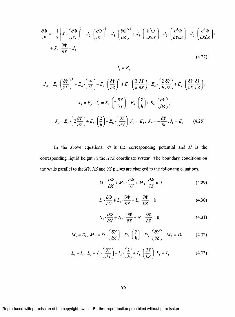
80 { (50 ) 2 (34 2 ao
J + at 2 I * (ax ) j2 a Y) j3 •
+J, ay +J8
J 2 - E i •
r ay )2
,ax + E 2 •
( 4"\
ft j
+ E 3
J 1 , E,,
( 4520 \ ,axay 1
+ J 5
( akp ayaz
J 6
a2,1),axaz
(4.27)
off 2
2 ay) r 2 ay) ( ay ay) ,7
L'4 h ax )± • --h az )± ,ax az )'
(
J 3 = E 3 , J 4 = El • 2 ay\ 2) ( ay` ax) + E4 •
(—h + E
6
•
az,
ay\ 2 a Y a Y J S =E3 •(2 +E5 • +E6 (—ax j,J 6 =E6 , =— ,J8 =E, (4.28)
az h i at
In the above equations, 0 is the corresponding potential and H is the
corresponding liquid height in the XYZ coordinate system. The boundary conditions on
the walls parallel to the XY, XZ and YZ planes are changed to the following equations.
acD acD acD Mi .— + M2 • —
a Y + M3 —
az =
ax 0
, i
ae. azi) L • — 1.2 • — /.3 —
ac =
ax a Y az
M, M2 , D,
al) a0 +N2 • — +N3 ac =0 ax a Y az
(a axn D2 1+D3 \a an , M3 = D3
( aY I I , L2 =I, • ,ax )+ I 2 PI+ 13 .1 ay\az
,L3 =1317)
96
(4.29)
(4.30)
(4.31)
(4.32)
(4.33)
Reproduced with permission of the copyright owner. Further reproduction prohibited without permission.
dt 2 ' 1
aov5X y
aoy d Y ;
+ J^ a o vva z y
+ J 4 ■r a 2o A
8 XdY+ J 5 ■
C \a odYdZ + J 6 '
/ 2,*x Aa o a x a z ,
r 5 0 r+ .Z7 b Jq1 b y 8
(4.27)
J\ = E X,
J 2 - E\ •r d Y vKdXj
+ E 2 •K ' l 2 J
+ is 3 •
ayva z y + A -
r i a y A v/* a x y
+ a^ 2 a y N\ h d Z j
+ Aay a r a x az
1 - F J - F*j j ^ 3 3 ^ 4 ^1' dY^v a x y \ h j
+ E<f dY \ d Z j
J S = E 3 ‘^2— V a z y + A -
' 2 N+ VV" /
"a y " va x y
,y6=£6, y 7= ~ , y 8=£7 (4.28)dt
In the above equations, 0 is the corresponding potential and H is the
corresponding liquid height in the XFZ coordinate system. The boundary conditions on
the walls parallel to the XY, X Z and YZ planes are changed to the following equations.
a o ao aoM, • - — + M7 • - — b M, • —— = 0ax ay az
(4.29)
a o _ ao aoL. ------ b Z,7 b L-, -----— 0a x
ao
ay J az
ao aoX, + N i + N i = 0ax ay az
M, = Z),, M 2 = D] • " ay "va x ,
+ a • f - 1 + A '^ a y Ava z y
, AZ3 = Z)3
(4.30)
(4.31)
(4.32)
L\ — 11 , L 2 — Z[ •r dY^ va x y
+ z2 •" 2 "
U , + Vr d Y )vazy A3=/ 3 (4.33)
96
Reproduced with permission of the copyright owner. Further reproduction prohibited without permission.
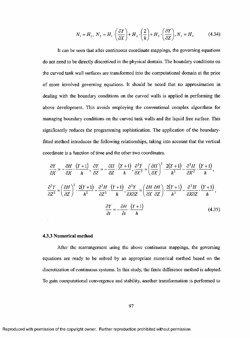
ay NI = Hi , N2 = H
' •(
ax)+ H
2 • i 2 \
\ j/ j+ H3
a (—
ayz ),N3 = H, (4.34)
It can be seen that after continuous coordinate mappings, the governing equations
do not need to be directly discretized in the physical domain. The boundary conditions on
the curved tank wall surfaces are transformed into the computational domain at the price
of more involved governing equations. It should be noted that no approximation in
dealing with the boundary conditions on the curved walls is applied in performing the
above development. This avoids employing the conventional complex algorithms for
managing boundary conditions on the curved tank walls and the liquid free surface. This
significantly reduces the programming sophistication. The application of the boundary-
fitted method introduces the following relationships, taking into account that the vertical
coordinate is a function of time and the other two coordinates.
aY ail (y +1) ay aH (y +1) a2Y —(ax)
H)2 2(y +1) a2H (y +1) ax ax h ' az az h 'axe ax h2 ax2 h '
a2y (aH )2 2(Y+1) a2H (Y+1) a2y (ail a 2(Y+1) 52H (Y+1) az2
- az h2 az2 h 'axaz ax az) h 2 axaz h '
8Y _ aH (Y+1) at at h
(4.35)
4.3.3 Numerical method
After the rearrangement using the above continuous mappings, the governing
equations are ready to be solved by an appropriate numerical method based on the
discretization of continuous systems. In this study, the finite difference method is adopted.
To gain computational convergence and stability, another transformation is performed to
97
Reproduced with permission of the copyright owner. Further reproduction prohibited without permission.
n x = h x, n 2 = h x-" d F N
+ h 2 ■' 2 s
+ H 3 ■{ d Y 12 J [ d Z ), n 3 = h 3 (4.34)
It can be seen that after continuous coordinate mappings, the governing equations
do not need to be directly discretized in the physical domain. The boundary conditions on
the curved tank wall surfaces are transformed into the computational domain at the price
o f more involved governing equations. It should be noted that no approximation in
dealing with the boundary conditions on the curved walls is applied in performing the
above development. This avoids employing the conventional complex algorithms for
managing boundary conditions on the curved tank walls and the liquid free surface. This
significantly reduces the programming sophistication. The application o f the boundary-
fitted method introduces the following relationships, taking into account that the vertical
coordinate is a function of time and the other two coordinates.
8 Y _ 8 H (F + l) 8 Y _ 8 H (F + l) 8 2Y _ f 8 H ) 2 2(Y + 1) d 2/ / (F + l)8 X 8 X
8 Y 8 Z 2
r 8 H} 2
k 8 Z j
8 Z 8 Z h 8X 2
2 (r + l) 8 2H ( f + i ) 8 2Y8 Z h 8 X 8 Z
8 Y _ _ _ 8 H_ (F + l) dt dt h
y d X y
8 H 8 H 8 X 8 Z
8 X 2
2(F + l) 8 2H (F + l)8 X 8 Z h
(4.35)
4.3.3 Numerical method
After the rearrangement using the above continuous mappings, the governing
equations are ready to be solved by an appropriate numerical method based on the
discretization of continuous systems. In this study, the finite difference method is adopted.
To gain computational convergence and stability, another transformation is performed to
97
Reproduced with permission of the copyright owner. Further reproduction prohibited without permission.
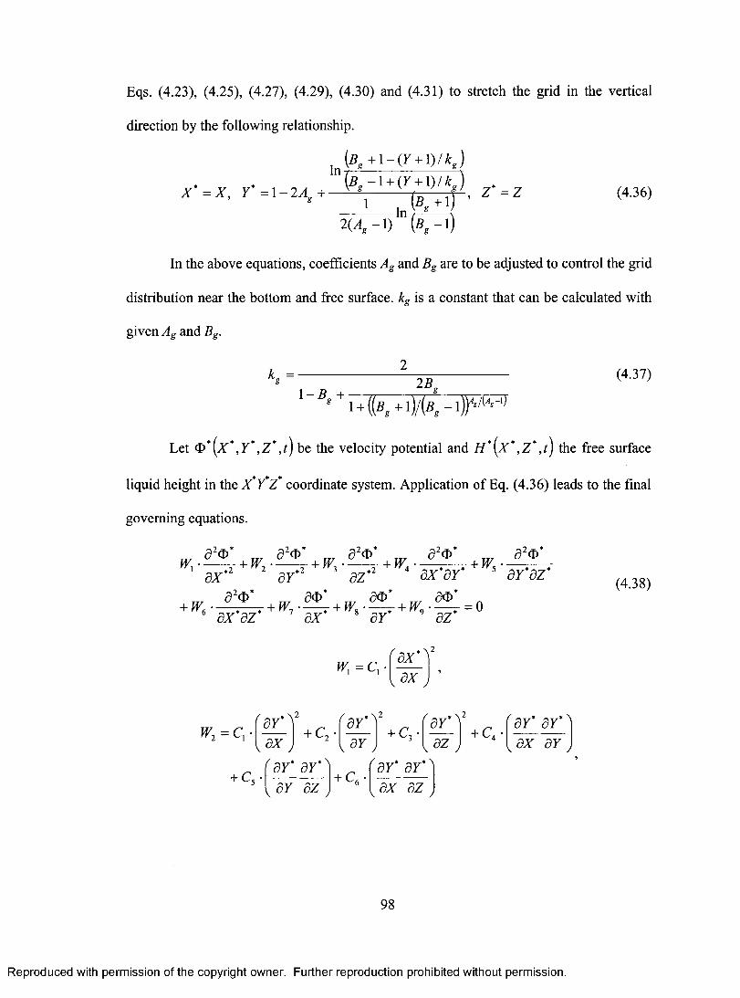
Eqs. (4.23), (4.25), (4.27), (4.29), (4.30) and (4.31) to stretch the grid in the vertical
direction by the following relationship.
,
In `Bg
+ 1 — (Y + 1) I kg)
(Bg —1+ (Y +1)I k‘g ) =1— 2Ag + 1
In(Bg +1) ' f \
2(A g —1) 0 ' g —1)
(4.36)
In the above equations, coefficients Ag and Bg are to be adjusted to control the grid
distribution near the bottom and free surface. kg is a constant that can be calculated with
given Ag and Bg.
kg = 2
2Bg
1— Bg +1+0 g +1)I(Bg — viig-i)
(4.37)
Let (13* (X ,Y , Z * ,t) be the velocity potential and H * (X * , Z * , t) the free surface
liquid height in the X*Y*Z* coordinate system. Application of Eq. (4.36) leads to the final
governing equations.
a 2 (1 )* a 2 * 82 cp* a 2,13* a 2,13*
W • +w2 • +w3 +w +w ax .2 aY*2 az .2 4 ax*aY* 5 aY*az*
2 * ao* ao* ao* +w • 6 ax*az
*+W' ax* +W8 a
* +W9 a*
=0
W 2 -= C i •
+ C 5
W, = C,
( * • \ 2 ( * )2 aY aY ' aY* 12
2 • 3 • pax + c + c , ,ay az'ay* aY* + C 'aye ay' ,aY az I
6 ax az 1
98
+ c 41 ay* ay*1
ax ay ) ,
(4.38)
Reproduced with permission of the copyright owner. Further reproduction prohibited without permission.
Eqs. (4.23), (4.25), (4.27), (4.29), (4.30) and (4.31) to stretch the grid in the vertical
direction by the following relationship.
, Z * = Z (4.36)X = X , Y = I - 2 A +( b +1)
2 ( A , - l ) lr,f c ^ T )
In the above equations, coefficients Ag and Bg are to be adjusted to control the grid
distribution near the bottom and free surface. kg is a constant that can be calculated with
given Ag and Bg.
k„ = 25(4.37)
g
l - B* + u
Let ®*(x*,r*,Z*,f) be the velocity potential and H*[x* ,Z * ,t) the free surface
liquid height in the X*r*Z* coordinate system. Application of Eq. (4.36) leads to the final
governing equations.
a2®* a 2®* a 2®* TT/ a 2®* a 2®W, + W , r- + W, T- + W , ; r + W.1 ax*2 2 ar*2 3 az*2 4 ax*ar* 5 a r ’az*
a2®* a®* a®* a®*+ w<- . . * +w1~ + w , - - — + w9- - — = 0e x az a x a r az
(4.38)
fr ,=c,r d x * v
\ dX ;
w2 = c x2
f2
f a r ’ ^2
f a r ’ a r ’ "j+ C, • + C3 • + c 4 *U x J U y J [ a z J s CD
ar* ar ar az
«\+ Q •
* \ar* ar ax az
98
Reproduced with permission of the copyright owner. Further reproduction prohibited without permission.
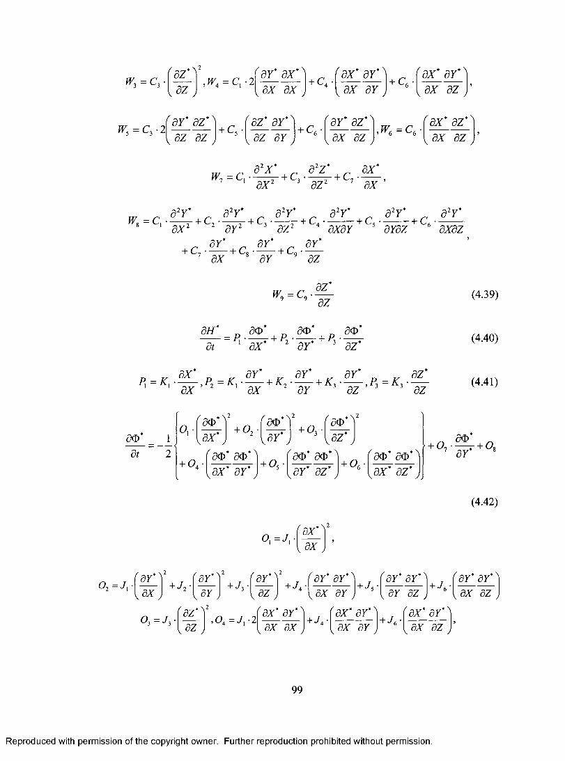
W3 = C3
W5 = C3 • 2
T478 = CI
'az' ,W4 = C, 2
'aY* az az az ,
+ C5
•ay* ax" • ax ax
az* ay*` az ay
+ C4
+ C6 •
'ax*aY*
ax ay ,
•ay* az*, ax az
( * *\ ax aY +C6
ax az
W6 =
a2x* a2z* ax w7 =c • +c • -pc axe az2 ax'
ax* az' ax az,
a2Y* a 2 y* a2Y* a 2 Y * a 2 Y * a 2 Y *
ax2 y2 az 2 + C4 aXa Y+ C5 a YaZ
+ C6 axaz
+C2 + C3
ay* ay* ay* +c, +c 8 + C9ax aY az
az*W9 = C9
az
aH*=P ao* + P • ao*+P ao*
• at ' ax* 2 aY* 3 az*
ax* ay* aY* ay* az P=K P =K • +K +K• P =K
' ax ' 2 I ax 2 aY 3 az ' 3 3 az
at 2 'ate* ao* + 05 ,ay* az* ,
'ate* ao* + 06 (ao
,ax* ate*
) * az*
7 + 0 80 Y
,ax* aY*
( * \ 2 ( * \ 2
+04
• 0* )2 +492 + o 3
ate* ax* aY* az*
(4.39)
(4.40)
(4.41)
0 2 = J, •
, ay* 12 (ayt y
,ax) + j2 +j3
0 l az. 1 23 = az '04=f'
(4.42)
ax*`2oi =J ' (ax ,
* ` 2
(ay* ay * ray * ay * ) ( ay * ay] • ay + j4 * ± 15* ay az )± j6 ax az az , , ax ay , 2(ax* ay*)
+J4 (ax* ay*)+J6 (
ax* ay*) ax ax ax ay ax az ,
99
Reproduced with permission of the copyright owner. Further reproduction prohibited without permission.
w3 = c 3-^az* ^2 v a Z y
, W . = C x-2 dY' dX* dX dX
+ C4 •* \ax* d r
dX dY+ C,
r dX* d Y ^
J
W5 = C3 • 2r dY* dZ*A
dZ dZ+ C5 -
Aaz* dY *A dZ dY
+ C,f dY* aZ*A
dX dZ,w6 = c 6
dX dZ
r d X ' dZ* ^
v dX dZ
w7 = c x + C3 . ^ + C7 •—7 1 a z 2 3 a z 2 7 ax
a2r* a 2r* a2r* a 2r* a 2r* a 2r* - c, • + c , • + c , • + c • + c , • + c .
a x 2 a r 2 a z 2 dXdY dYdZ axaz
+ c , - — + c„- — + c 0 a rax a r
wg = c 9-
az
az*az
a#* n ao* „ ao* „ ao* = p •— - t + p , - — ^ + p , -
dt ax ar* az
= X, . — , p , = K t - ^ r + X, - ^ - + K ^ ^ — ,P ,= K dZ1 1 a x ’ 2 ax a r az az
(4.39)
(4.40)
(4.41)
ao <V/ » A2ao
ax*
/ \ 2 aova r y
^ a o * ^ 2vaz y
dt 2 ( ao* ao* "i f a o ’ ao* 'I f ao* ao* ^+ Oa * + Oc * + Os *
% CD [ar* a z ’ J [ax* a z ’ J
ao+ o 7 ~ + o 8
7 a r 8
(4.42)
Ox= J x ax*v a x y
o 2Aa r* ^ 2v a x y
+ «/*> 'dy*" '2v a r y
r dY^ 2
\ d Z y+ Ji
r dY' a r * A ax a r +J<
r 8 Y* ar*^ a r az
Aar* ar*" ax az ,
o 3 = j 3 -^az*^2v a z y
, 0 4 = J X-2r a x ’ ar* 'I f ax* ar* 'I f ax* ar* 'I+ J 4 ‘ + J 6 '
[ a x ax J [ a x a r J [ a x az J
99
Reproduced with permission of the copyright owner. Further reproduction prohibited without permission.
OZ* OY*O5 = J
3 • 2( . az)+ J
5
'az* ay'\ az ay j+.16
'az* ay*) n T (ax* az* 3 3-0'6 - a 6 3
az ax ax az
ay* aY* 0, = J 7 ay at , 0 8 = J 8 (4.43)
The boundary conditions on the walls parallel to the X*Y* plane, X*Z* plane and
I/Z* plane are changed to the following.
a o* ate* a es* S'
+s +s =0 1 ax* 2 ay' az*
, ao* , aci* acb* v, ax*
+Q2 ay* +Q3 az* = 0
ao* ao* ao* R1 ax* + R2 ay* + R3 az*
=0
ax* ay* ay ay az s,=m, • , S2 = MI • +M2 +M3 , S3 = M3ax ax OY az az
ay* ay* ay* az* Q, = LI • —
ax* , Q2 = L, • +L2' +L3. , Q3 = L3ax ax aY az az
ax aY* ay* ay* az*R, = N 1 — , R2 = N, • + N2 + N3 , R3 = N3
ax ax aY az az
(4.44)
(4.45)
(4.46)
(4.47)
(4.48)
(4.49)
The following relationships can be obtained with the application of the boundary-
fitted method.
ay* ay* ay ay* ay* ay ay* ay* aY = ax ay ax 5 3 az ay az at ay at 5
a2Y* _ a2Y* ( ay ) +
2 ay* a2Y a2Y* = a2Y* ( 3)12 +
ay* a2Yax2 aY2 .aAT aY ax2 ' az2 aY2 .3z ) ay aZ2 '
a2Y* a2Y* axaz = aY2
( ay ay) ay* a2Y ax az + ay axaz'
100
Reproduced with permission of the copyright owner. Further reproduction prohibited without permission.
Os = J 3-2r dZ* 3Y*A
dZ dZ+ Jc f dZ' ar*A
dZ dY + -Vf dZ* dY*A
8 Z dX ’Of, — Jf,r dx' d z ^
dx dz
O - J .2L . . 2L o = j'-/7 ~ J l _ 9^8 ^8 (4.43)dY dt
The boundary conditions on the walls parallel to the X*Y* plane, X*Z* plane and
Y*Z* plane are changed to the following.
ao*ao ao s r ^ + s 2 - ^ 1 ax 2 ar + s 3 ■az = 0
_ ao* ao* ao*Q\ ’ — r Qi — *■ Q-i — *■_ 0
1 dX 2 dY 3 a z
ax ar* az*
(4.44)
(4.45)
(4.46)
_ ax _ .. ar ar .. ar _ .. az5, = M , -------,S 2 - M , -------- yM 2 ------- h M ,------ , S , = M ,------ (4.47)1 1 ax ax 2 ar 3 az 3 3 az
_ r ax* T ar* r ar* , ar* r az*Q\ — L\ > Q? — A 1- L2 1- L , , Q-, — L-,------1 ' a x 2 1 ax 2 ar 3 az 3 3 az
= n x■— ,R 2 = N i • — + x 2 1 1 ax 2 1 ax 2az*d . . 1- N-,------ , R-, — N-,------ar 3 az 3 3 az
(4.48)
(4.49)
The following relationships can be obtained with the application of the boundary-
fitted method.
ar _aT ar ar _aT ar ar _aT ardX ~ dY ' d X ’ dZ ~ dY ' d Z ’ dt ~ dY ' dt ’
a2r* a2r* farY . ar* a2r a2r* a2r* farY ar* a2rax2 ar2
ar* a2r a2r* _ a2r* "ar tUxJ ar ax2 ’ az2 ar2 UzJ ar dz2
a2r* _a2r* far ar\ ar a2r axaz_ ar2 'laxaz J+ ar ’axaz
100
Reproduced with permission of the copyright owner. Further reproduction prohibited without permission.
a2y* a2y* ay 52y* 52y* ay
axay ay2 ax' ayaz ay2 az'
aH air ax* aH ail az* ax ax* ax' az az* az'
52x 52x* ax*'2 ax* 52x*` 52x 52x* (at"' ax* (52Z*(4.50)
ax2 ax*2 ax +
ax*
ax2 az2 az*2 az , +
az*
,az2
4.3.4 Calculation procedures
The calculation procedures are exactly the same as those described in Section 3.3,
except that all quantities should be calculated in both lateral and longitudinal directions,
as the liquid motion is modeled in 3D space. The metrics of the velocity potential in the
rearranged governing equations are now written using the followings expressions.
a24)* (-13,7+,,k ax
*2 = (Ax *Y 520* 0:,j •+1,k —20:,J.k + (1)i,j-1,k =
ay *2 ry
520* cD*. — 2cD1*. + cDis,j,k ,j,k-1
az *2 (A7*Y * a20* 1:13 * * * i+1, j+1,k + 43 —43.i-1,j-1,k i+1,j-1,k — 43
aX * ar 4AX*AY*
azo* cD* + cD* — cD* — cD*i+1,j,k+1 i-1,j,k-I i+1,j,k-1 i-1,j,k+1
ax*az* 4AX*A7*
(13a2cD * * + * . — cro* . 4:)i,J+1,k+1 — o i*,j-1,k+1 ar aZ * 4A Y*A7*
101
(4.51)
(4.52)
(4.53)
(4.54)
(4.55)
(4.56)
Reproduced with permission of the copyright owner. Further reproduction prohibited without permission.
8 2Y 8 2Y dY 8 2Y d 2Y dYa XdY d Y 2 8X ’ 8 Y8 Z d Y 2 8 Z
8 H 8 H * dX* 8 H 8 H * 8 Z*s x d x * a x ’ az az* az ’
8 2h 8 2h * fa x * va x 2 ax*2 v a x y
a //ax*
^ a 2x * A a x 2
a 2/ / a 2/ / r 8 Z *^2
s z 2 az* v az ,+-
a //az*
( a 2z*^ v a z 2 y
(4.50)
4.3.4 Calculation procedures
The calculation procedures are exactly the same as those described in Section 3.3,
except that all quantities should be calculated in both lateral and longitudinal directions,
as the liquid motion is modeled in 3D space. The metrics of the velocity potential in the
rearranged governing equations are now written using the followings expressions.
a2o* _ o *+U;4-2(D*7, , + o *_1i (4 5i)
(4.52)
(4.53)
(4.54)
(4.55)
(4.56)
ax*2 (AX*)2
a2®* _ ®U+U - 2< , * + ® u -uar*2 (AT*)2
a 2®* + <M -.az*2 (az*)2
aX*aZ* 4AX*A 7*
a2®* _ + K um-x ~ ,4+1
ax*az*
a2®*ar*az*
4 AX AZ
® i , . / + l , 4 + l + ® i , y - l , 4 - l ^ i .j + 1,4 -1 ^ i ' J - 1 , 4 + 1
4AF AZ
101
Reproduced with permission of the copyright owner. Further reproduction prohibited without permission.
ac* ax* 2AX*
a _ i,j+1,k (1);,j-1,k
ay* 2AY*
ac)* _€13
az* — 2AZ*
On the boundaries:
ao* + 40*2,J,k -03,J,k ax* 2AX*
* * ao _ — 30*N+1,J,k + 4(1) N,J,k — 0 ;1_1, ,k) ax* 2AX*
ao* 30, Ik + 40,2,k 0,3,k a Y* 2AY*
ao = - 443:,M,k -413i,M-1,k)
ay* 2AY*
ao* _ + 4o*„.,,2 az* 2AZ*
ate* 3(1)* + 407 — (1)t.
i,j,L+1 t,j,L ,j,L-1
az* 2AZ*
(4.57)
(4.58)
(4.59)
(4.60)
(4.61)
(4.62)
(4.63)
(4.64)
(4.65)
The metrics of the liquid height in the rearranged governing equations are written
by the followings expressions.
ax 11:+i k — H: k , - ,
ax* 2AX*
a2 H* = H: +1,k 211,:k H: Lk
ax*2 (Ax*)2
—
aH + 4.1-1; k — H3* k
ax* 2AX*
102
(4.66)
(4.67)
(4.68)
Reproduced with permission of the copyright owner. Further reproduction prohibited without permission.
d x 2 AX
5 0 O iy+l k — O, j_x k8 Y 2AY
5 0 _ Q;j,*+i ~ Oi,y,t-i a z ^ - 2AZ*
On the boundaries:
a o ’ - 3 0 ^ + 4 0 ^ - 0 ^ax* 2 AX*
c"t.’ - (- - ^V iJ t )ax* 2 AX*
ao* _ - 3 0 * u + 40* 2i - 0 *3
ar 2a f
5 0 _ ~ (~ 3 Q / A/+l t + 4 Q ;M t ~Q),a/-i,^) ar* “ 2Ar*
ao* - 3Q/JJ + 40*ji2 - O/j.3 az* 2AZ*
ao* - ( - 3 0 * j .i+1+ 4 0 ’M - 0 * 7.i . 1)
(4.57)
(4.58)
(4.59)
(4.60)
(4.61)
(4.62)
(4.63)
(4.64)
(4.65)az 2AZ
The metrics of the liquid height in the rearranged governing equations are written
by the followings expressions.
a //’ _ h ;+1, - H*_l kax* 2 AX*
a 2//*ax*2 (ax*)2
a//* _ -3H*l k + 4 H ’2 k - H l k ax* 2 AX*
102
(4.66)
(4.67)
(4.68)
Reproduced with permission of the copyright owner. Further reproduction prohibited without permission.
OH* ( 3H- N. 4eN,k eN-1,k ax* 26,A' *
all* —
, I I k+1 H ,k-1
az* 2AZ*
a211* *k+l - 2H ,*k =
az*2 (Az * )2
_ + 4HL — H i: 3
az* 2A7*
art _—(-31-1,7,L+1+ az* 2A7*
(4.69)
(4.70)
(4.71)
(4.72)
(4.73)
4.4 Results and discussion
4.4.1 Natural frequencies
Knowledge of the natural frequencies of liquid sloshing in horizontal cylindrical
tanks is important in designing and manufacturing liquid cargo tanks and their supporting
structures. Identification of the natural frequencies may help to avoid the oscillation that
leads to large-amplitude fluid motion, which causes vehicle instability and even structural
failure. The mathematical method for the natural frequencies of liquid motion in 2D
circular and elliptical tanks developed in the previous chapter can be extended to solve
the natural frequencies of liquid motion in 3D cylindrical tanks. A linearized Bernoulli
equation on the free surface and the governing equations inside the liquid domain and on
the rigid walls lead to a generalized eigenvalue problem. The procedures used in the
previous chapter can be easily applied by increasing the third dimension in the
longitudinal direction and solving this problem in a 3D space.
Theoretical solutions for longitudinal sloshing frequency and liquid motion have
103
Reproduced with permission of the copyright owner. Further reproduction prohibited without permission.
(4.69)dX 2AX
(4.70)8Z* 2AZ*
(4.71)az*2 (a z *)2
(4.72)
(4.73)dZ 2AZ
4.4 Results and discussion
4.4.1 Natural frequencies
Knowledge o f the natural frequencies o f liquid sloshing in horizontal cylindrical
tanks is important in designing and manufacturing liquid cargo tanks and their supporting
structures. Identification o f the natural frequencies may help to avoid the oscillation that
leads to large-amplitude fluid motion, which causes vehicle instability and even structural
failure. The mathematical method for the natural frequencies o f liquid motion in 2D
circular and elliptical tanks developed in the previous chapter can be extended to solve
the natural frequencies o f liquid motion in 3D cylindrical tanks. A linearized Bernoulli
equation on the free surface and the governing equations inside the liquid domain and on
the rigid walls lead to a generalized eigenvalue problem. The procedures used in the
previous chapter can be easily applied by increasing the third dimension in the
longitudinal direction and solving this problem in a 3D space.
Theoretical solutions for longitudinal sloshing frequency and liquid motion have
103
Reproduced with permission of the copyright owner. Further reproduction prohibited without permission.
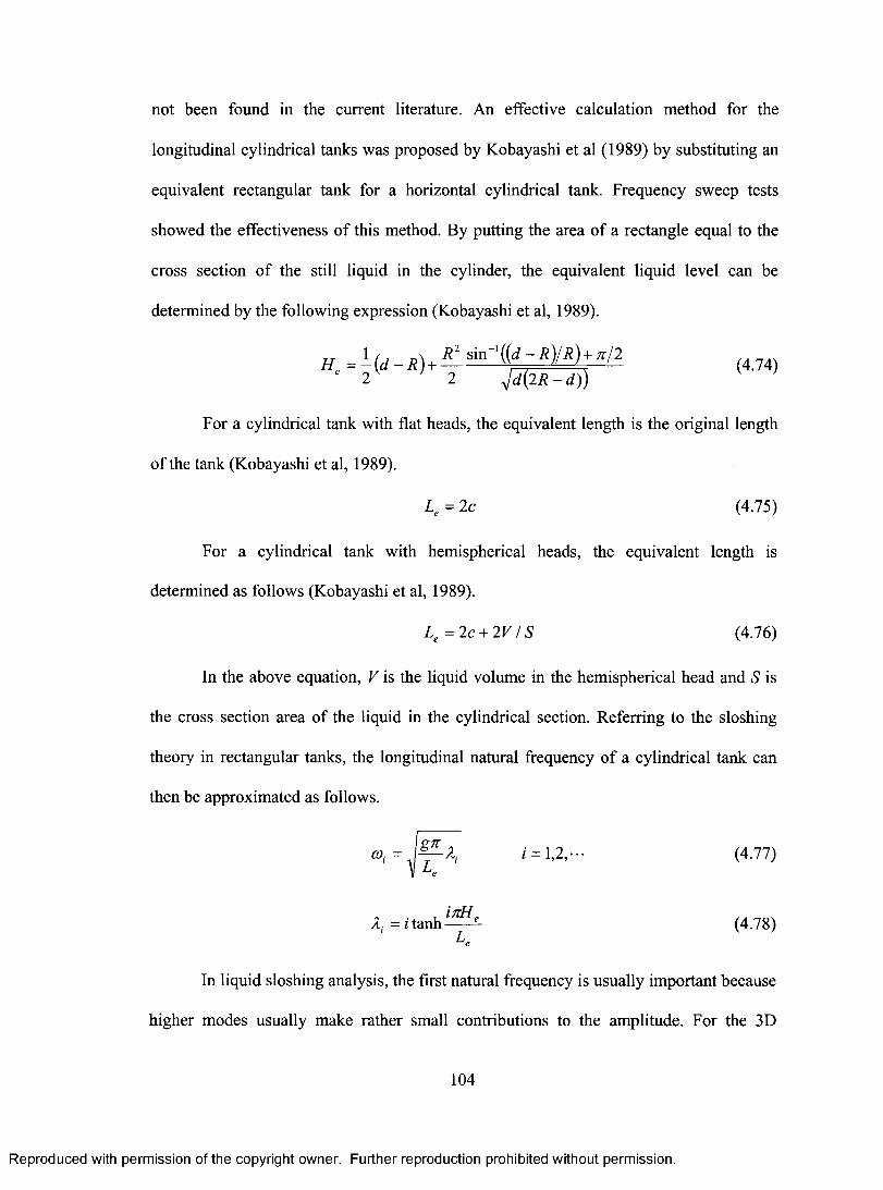
not been found in the current literature. An effective calculation method for the
longitudinal cylindrical tanks was proposed by Kobayashi et al (1989) by substituting an
equivalent rectangular tank for a horizontal cylindrical tank. Frequency sweep tests
showed the effectiveness of this method. By putting the area of a rectangle equal to the
cross section of the still liquid in the cylinder, the equivalent liquid level can be
determined by the following expression (Kobayashi et al, 1989).
1 1 \ — OR)+ rc12 H = - R)+ e 2 2 ild(2R— d))
(4.74)
For a cylindrical tank with flat heads, the equivalent length is the original length
of the tank (Kobayashi et al, 1989).
Le = 2c (4.75)
For a cylindrical tank with hemispherical heads, the equivalent length is
determined as follows (Kobayashi et al, 1989).
Le =2c +2V I S (4.76)
In the above equation, V is the liquid volume in the hemispherical head and S is
the cross section area of the liquid in the cylindrical section. Referring to the sloshing
theory in rectangular tanks, the longitudinal natural frequency of a cylindrical tank can
then be approximated as follows.
co, = gg
i = 1,2, • • • (4.77) Le
A, =itanh Le
(4.78)
In liquid sloshing analysis, the first natural frequency is usually important because
higher modes usually make rather small contributions to the amplitude. For the 3D
104
Reproduced with permission of the copyright owner. Further reproduction prohibited without permission.
not been found in the current literature. An effective calculation method for the
longitudinal cylindrical tanks was proposed by Kobayashi et al (1989) by substituting an
equivalent rectangular tank for a horizontal cylindrical tank. Frequency sweep tests
showed the effectiveness o f this method. By putting the area o f a rectangle equal to the
cross section o f the still liquid in the cylinder, the equivalent liquid level can be
determined by the following expression (Kobayashi et al, 1989).
For a cylindrical tank with flat heads, the equivalent length is the original length
o f the tank (Kobayashi et al, 1989).
4 = 2c (4.75)
For a cylindrical tank with hemispherical heads, the equivalent length is
determined as follows (Kobayashi et al, 1989).
Le =2c + 2 V I S (4.76)
In the above equation, V is the liquid volume in the hemispherical head and S is
the cross section area o f the liquid in the cylindrical section. Referring to the sloshing
theory in rectangular tanks, the longitudinal natural frequency o f a cylindrical tank can
then be approximated as follows.
4 = i tanh *n^ e- (4.78)
In liquid sloshing analysis, the first natural frequency is usually important because
higher modes usually make rather small contributions to the amplitude. For the 3D
104
Reproduced with permission of the copyright owner. Further reproduction prohibited without permission.
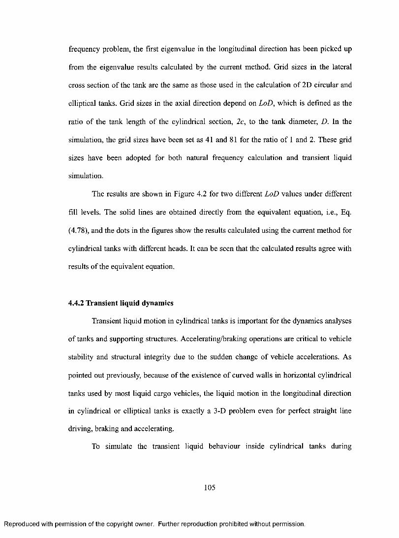
frequency problem, the first eigenvalue in the longitudinal direction has been picked up
from the eigenvalue results calculated by the current method. Grid sizes in the lateral
cross section of the tank are the same as those used in the calculation of 2D circular and
elliptical tanks. Grid sizes in the axial direction depend on LoD, which is defined as the
ratio of the tank length of the cylindrical section, 2c, to the tank diameter, D. In the
simulation, the grid sizes have been set as 41 and 81 for the ratio of 1 and 2. These grid
sizes have been adopted for both natural frequency calculation and transient liquid
simulation.
The results are shown in Figure 4.2 for two different LoD values under different
fill levels. The solid lines are obtained directly from the equivalent equation, i.e., Eq.
(4.78), and the dots in the figures show the results calculated using the current method for
cylindrical tanks with different heads. It can be seen that the calculated results agree with
results of the equivalent equation.
4.4.2 Transient liquid dynamics
Transient liquid motion in cylindrical tanks is important for the dynamics analyses
of tanks and supporting structures. Accelerating/braking operations are critical to vehicle
stability and structural integrity due to the sudden change of vehicle accelerations. As
pointed out previously, because of the existence of curved walls in horizontal cylindrical
tanks used by most liquid cargo vehicles, the liquid motion in the longitudinal direction
in cylindrical or elliptical tanks is exactly a 3-D problem even for perfect straight line
driving, braking and accelerating.
To simulate the transient liquid behaviour inside cylindrical tanks during
105
Reproduced with permission of the copyright owner. Further reproduction prohibited without permission.
frequency problem, the first eigenvalue in the longitudinal direction has been picked up
from the eigenvalue results calculated by the current method. Grid sizes in the lateral
cross section of the tank are the same as those used in the calculation of 2D circular and
elliptical tanks. Grid sizes in the axial direction depend on LoD, which is defined as the
ratio o f the tank length of the cylindrical section, 2c, to the tank diameter, D. In the
simulation, the grid sizes have been set as 41 and 81 for the ratio o f 1 and 2. These grid
sizes have been adopted for both natural frequency calculation and transient liquid
simulation.
The results are shown in Figure 4.2 for two different LoD values under different
fill levels. The solid lines are obtained directly from the equivalent equation, i.e., Eq.
(4.78), and the dots in the figures show the results calculated using the current method for
cylindrical tanks with different heads. It can be seen that the calculated results agree with
results o f the equivalent equation.
4.4.2 Transient liquid dynamics
Transient liquid motion in cylindrical tanks is important for the dynamics analyses
of tanks and supporting structures. Accelerating/braking operations are critical to vehicle
stability and structural integrity due to the sudden change of vehicle accelerations. As
pointed out previously, because of the existence of curved walls in horizontal cylindrical
tanks used by most liquid cargo vehicles, the liquid motion in the longitudinal direction
in cylindrical or elliptical tanks is exactly a 3-D problem even for perfect straight line
driving, braking and accelerating.
To simulate the transient liquid behaviour inside cylindrical tanks during
105
Reproduced with permission of the copyright owner. Further reproduction prohibited without permission.
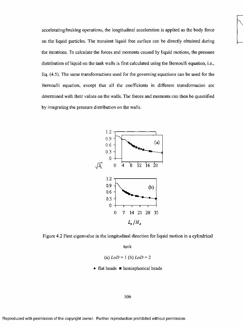
accelerating/braking operations, the longitudinal acceleration is applied as the body force
on the liquid particles. The transient liquid free surface can be directly obtained during
the iterations. To calculate the forces and moments caused by liquid motions, the pressure
distribution of liquid on the tank walls is first calculated using the Bernoulli equation, i.e.,
Eq. (4.5). The same transformations used for the governing equations can be used for the
Bernoulli equation, except that all the coefficients in different transformation are
determined with their values on the walls. The forces and moments can then be quantified
by integrating the pressure distribution on the walls.
1.2
0.9 0.6
(a)
0.3
0
4 8 I 12
I I 16 20 j 0
1.2
0.9 - (b) 0.6 -
0.3 -
0
0 7 14 21 28 35
Le /He
Figure 4.2 First eigenvalue in the longitudinal direction for liquid motion in a cylindrical
tank
(a) LoD = 1 (b) LoD = 2
• flat heads • hemispherical heads
106
Reproduced with permission of the copyright owner. Further reproduction prohibited without permission.
accelerating/braking operations, the longitudinal acceleration is applied as the body force
on the liquid particles. The transient liquid free surface can be directly obtained during
the iterations. To calculate the forces and moments caused by liquid motions, the pressure
distribution of liquid on the tank walls is first calculated using the Bernoulli equation, i.e.,
Eq. (4.5). The same transformations used for the governing equations can be used for the
Bernoulli equation, except that all the coefficients in different transformation are
determined with their values on the walls. The forces and moments can then be quantified
by integrating the pressure distribution on the walls.
1 .2 ----------------------------0.9 - 0.6 -
0.3 -‘0 -
^ 0 4 8 12 16 20
1.2 -
0.9 - 0.6 -
0.3 -i-0 -
0 7 14 21 28 35
h i n .
Figure 4.2 First eigenvalue in the longitudinal direction for liquid motion in a cylindrical
tank
(a) LoD = 1 (b) LoD = 2
• flat heads ■ hemispherical heads
106
Reproduced with permission of the copyright owner. Further reproduction prohibited without permission.
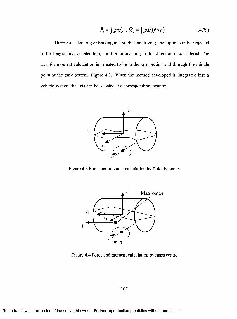
Fl = f(pds)ii , A = f(pds)(7- x ii) (4.79)
During accelerating or braking in straight-line driving, the liquid is only subjected
to the longitudinal acceleration, and the force acting in this direction is considered. The
axis for moment calculation is selected to be in the x1 direction and through the middle
point at the tank bottom (Figure 4.3). When the method developed is integrated into a
vehicle system, the axis can be selected at a corresponding location.
z1
Figure 4.3 Force and moment calculation by fluid dynamics
Mass centre
Figure 4.4 Force and moment calculation by mass centre
107
Reproduced with permission of the copyright owner. Further reproduction prohibited without permission.
F; = ^(pds)n , M, = ^{pds\r x n) (4.79)
During accelerating or braking in straight-line driving, the liquid is only subjected
to the longitudinal acceleration, and the force acting in this direction is considered. The
axis for moment calculation is selected to be in the x\ direction and through the middle
point at the tank bottom (Figure 4.3). When the method developed is integrated into a
vehicle system, the axis can be selected at a corresponding location.
Figure 4.3 Force and moment calculation by fluid dynamics
Mass centre
Figure 4.4 Force and moment calculation by mass centre
107
Reproduced with permission of the copyright owner. Further reproduction prohibited without permission.
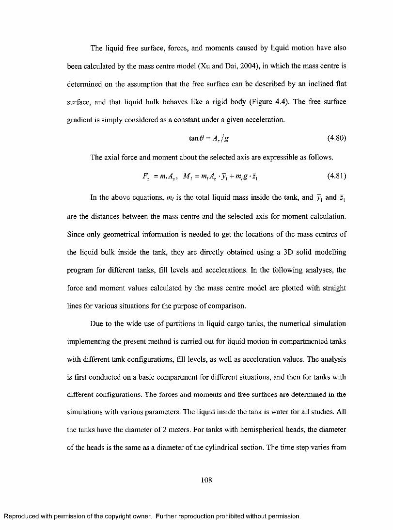
The liquid free surface, forces, and moments caused by liquid motion have also
been calculated by the mass centre model (Xu and Dai, 2004), in which the mass centre is
determined on the assumption that the free surface can be described by an inclined flat
surface, and that liquid bulk behaves like a rigid body (Figure 4.4). The free surface
gradient is simply considered as a constant under a given acceleration.
tan 0 = A, /g (4.80)
The axial force and moment about the selected axis are expressible as follows.
F. = mi Az , M1 = mi Az • A + mig • f 1 (4.81)
In the above equations, in/ is the total liquid mass inside the tank, and y, and f l
are the distances between the mass centre and the selected axis for moment calculation.
Since only geometrical information is needed to get the locations of the mass centres of
the liquid bulk inside the tank, they are directly obtained using a 3D solid modelling
program for different tanks, fill levels and accelerations. In the following analyses, the
force and moment values calculated by the mass centre model are plotted with straight
lines for various situations for the purpose of comparison.
Due to the wide use of partitions in liquid cargo tanks, the numerical simulation
implementing the present method is carried out for liquid motion in compartmented tanks
with different tank configurations, fill levels, as well as acceleration values. The analysis
is first conducted on a basic compartment for different situations, and then for tanks with
different configurations. The forces and moments and free surfaces are determined in the
simulations with various parameters. The liquid inside the tank is water for all studies. All
the tanks have the diameter of 2 meters. For tanks with hemispherical heads, the diameter
of the heads is the same as a diameter of the cylindrical section. The time step varies from
108
Reproduced with permission of the copyright owner. Further reproduction prohibited without permission.
The liquid free surface, forces, and moments caused by liquid motion have also
been calculated by the mass centre model (Xu and Dai, 2004), in which the mass centre is
determined on the assumption that the free surface can be described by an inclined flat
surface, and that liquid bulk behaves like a rigid body (Figure 4.4). The free surface
gradient is simply considered as a constant under a given acceleration.
tan 6 = A j g (4.80)
The axial force and moment about the selected axis are expressible as follows.
FZ| = m,Az, M, = m,Az -y, + m ,g - z l (4.81)
In the above equations, mi is the total liquid mass inside the tank, and y, and z,
are the distances between the mass centre and the selected axis for moment calculation.
Since only geometrical information is needed to get the locations o f the mass centres of
the liquid bulk inside the tank, they are directly obtained using a 3D solid modelling
program for different tanks, fill levels and accelerations. In the following analyses, the
force and moment values calculated by the mass centre model are plotted with straight
lines for various situations for the purpose o f comparison.
Due to the wide use of partitions in liquid cargo tanks, the numerical simulation
implementing the present method is carried out for liquid motion in compartmented tanks
with different tank configurations, fill levels, as well as acceleration values. The analysis
is first conducted on a basic compartment for different situations, and then for tanks with
different configurations. The forces and moments and free surfaces are determined in the
simulations with various parameters. The liquid inside the tank is water for all studies. All
the tanks have the diameter o f 2 meters. For tanks with hemispherical heads, the diameter
o f the heads is the same as a diameter o f the cylindrical section. The time step varies from
108
Reproduced with permission of the copyright owner. Further reproduction prohibited without permission.
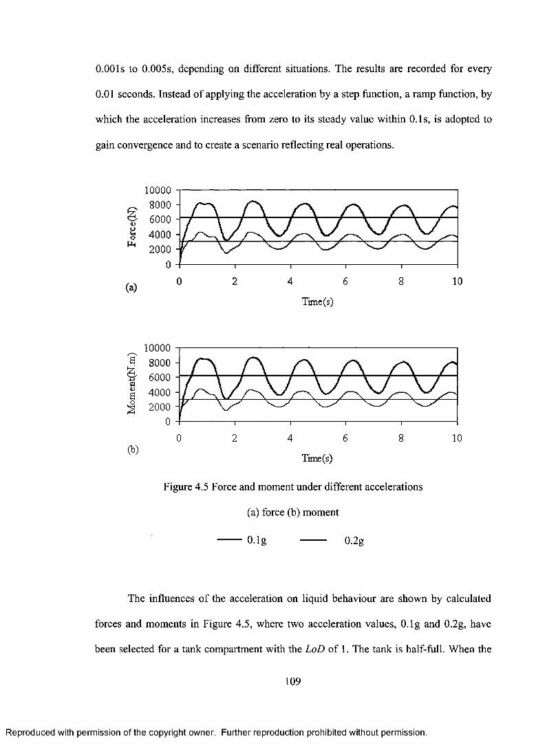
0.001s to 0.005s, depending on different situations. The results are recorded for every
0.01 seconds. Instead of applying the acceleration by a step function, a ramp function, by
which the acceleration increases from zero to its steady value within 0.1s, is adopted to
gain convergence and to create a scenario reflecting real operations.
(a)
10000
8000 6000
4000 2000
0
0
10000
8000 V 6000
4000 2000
0
0 (b)
2 4 6
Time(s)
8 10
2 4 6
Time (s)
8
Figure 4.5 Force and moment under different accelerations
(a) force (b) moment
0.1g 0.2g
10
The influences of the acceleration on liquid behaviour are shown by calculated
forces and moments in Figure 4.5, where two acceleration values, 0.1g and 0.2g, have
been selected for a tank compartment with the LoD of 1. The tank is half-full. When the
109
Reproduced with permission of the copyright owner. Further reproduction prohibited without permission.
0.001s to 0.005s, depending on different situations. The results are recorded for every
0.01 seconds. Instead of applying the acceleration by a step function, a ramp function, by
which the acceleration increases from zero to its steady value within 0.1s, is adopted to
gain convergence and to create a scenario reflecting real operations.
<L)OUo
(a)
100008000600040002000
0
2 6 80 4 10
Time(s)
a&+->C<DaO
(b)
100008000600040002000
00 2 4 6 8 10
Time(s)
Figure 4.5 Force and moment under different accelerations
(a) force (b) moment
O.lg ------- 0.2g
The influences o f the acceleration on liquid behaviour are shown by calculated
forces and moments in Figure 4.5, where two acceleration values, O.lg and 0.2g, have
been selected for a tank compartment with the LoD of 1. The tank is half-full. When the
109
Reproduced with permission of the copyright owner. Further reproduction prohibited without permission.
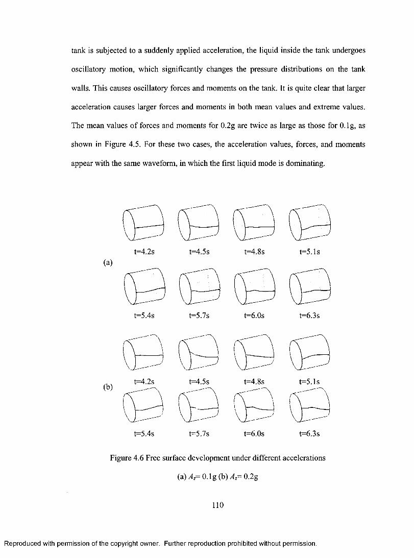
tank is subjected to a suddenly applied acceleration, the liquid inside the tank undergoes
oscillatory motion, which significantly changes the pressure distributions on the tank
walls. This causes oscillatory forces and moments on the tank. It is quite clear that larger
acceleration causes larger forces and moments in both mean values and extreme values.
The mean values of forces and moments for 0.2g are twice as large as those for 0.1g, as
shown in Figure 4.5. For these two cases, the acceleration values, forces, and moments
appear with the same waveform, in which the first liquid mode is dominating.
(a)
(b)
t=4.2s
t=5.4s
t=4.2s
t=5.4s
t=4.5 s
t=5.7s
t=4.5 s
t=5 .7 s
t=4.8s
t=6.0s
t=4.8s
t=6.0s
t=5.1s
t=6.3s
t=5.1s
t=6.3s
Figure 4.6 Free surface development under different accelerations
(a) AZ 0.1g (b) AZ 0.2g
110
Reproduced with permission of the copyright owner. Further reproduction prohibited without permission.
tank is subjected to a suddenly applied acceleration, the liquid inside the tank undergoes
oscillatory motion, which significantly changes the pressure distributions on the tank
walls. This causes oscillatory forces and moments on the tank. It is quite clear that larger
acceleration causes larger forces and moments in both mean values and extreme values.
The mean values o f forces and moments for 0.2g are twice as large as those for O.lg, as
shown in Figure 4.5. For these two cases, the acceleration values, forces, and moments
appear with the same waveform, in which the first liquid mode is dominating.
t=4.2s(a)
t=5.4s
t=4.5s
t=5.7s
t=4.8s
t=6.0s
t=5.1s
t=6.3s
t=4.2s(b)
t=5.4s
t=4.5s t=4.8s
\
t=5.1s
t=5.7s t=6.0s t=6.3s
Figure 4.6 Free surface development under different accelerations
(a) Az= O.lg (b) Az= 0.2g
110
Reproduced with permission of the copyright owner. Further reproduction prohibited without permission.
Corresponding free surface development is illustrated in Figure 4.6 at different
times. It can be found that the free surfaces evolve in a similar manner for both
acceleration values, except that the liquid heights on the walls are higher under larger
acceleration. It can be seen from the figure that at most of the times, the free surfaces are
no longer inclined flat surfaces, even though the first natural liquid mode is dominating.
Higher modes are superposed on the first mode, a situation which is clearly shown by the
free surface shapes. For such a short tank compartment, the liquid motion takes the form
of standing waves.
The influence of fill levels on the liquid motion inside the same tank is studied by
comparing the forces and moments on the tank walls when the fill levels are 0.4D and
0.6D. This comparison is exhibited in Figure 4.7. As can be seen from Figure 4.7, the
force and moment have larger mean values at a fill level of 0.6D due to more liquid
inside the tank at a higher fill level. At the same time, the variations of force and moment
at 0.6D have smaller periods due to the increase in frequency caused by the higher fill
level.
Figure 4.8 shows the forces and moments of three different tanks to investigate
the influence of the hemispherical heads on the transient liquid behaviour. The tanks are
all half-full and the acceleration is 0.1g. Due to the different lengths of the tanks, the
periods of the three tanks are different. The longest tank has the largest period. The mean
values and the alternating values of oscillatory forces and moments are also different. The
values for the second and third tanks are much larger than those of the first tank, due to
their larger liquid volumes. It can be found from this figure that the force and moment
characteristics of the tank with hemispherical heads are much closer to those of the tank
111
Reproduced with permission of the copyright owner. Further reproduction prohibited without permission.
Corresponding free surface development is illustrated in Figure 4.6 at different
times. It can be found that the free surfaces evolve in a similar manner for both
acceleration values, except that the liquid heights on the walls are higher under larger
acceleration. It can be seen from the figure that at most o f the times, the free surfaces are
no longer inclined flat surfaces, even though the first natural liquid mode is dominating.
Higher modes are superposed on the first mode, a situation which is clearly shown by the
free surface shapes. For such a short tank compartment, the liquid motion takes the form
of standing waves.
The influence of fill levels on the liquid motion inside the same tank is studied by
comparing the forces and moments on the tank walls when the fill levels are 0.4D and
0.6D. This comparison is exhibited in Figure 4.7. As can be seen from Figure 4.7, the
force and moment have larger mean values at a fill level o f 0.6D due to more liquid
inside the tank at a higher fill level. At the same time, the variations o f force and moment
at 0.6D have smaller periods due to the increase in frequency caused by the higher fill
level.
Figure 4.8 shows the forces and moments o f three different tanks to investigate
the influence of the hemispherical heads on the transient liquid behaviour. The tanks are
all half-full and the acceleration is O.lg. Due to the different lengths o f the tanks, the
periods o f the three tanks are different. The longest tank has the largest period. The mean
values and the alternating values o f oscillatory forces and moments are also different. The
values for the second and third tanks are much larger than those o f the first tank, due to
their larger liquid volumes. It can be found from this figure that the force and moment
characteristics o f the tank with hemispherical heads are much closer to those of the tank
111
Reproduced with permission of the copyright owner. Further reproduction prohibited without permission.
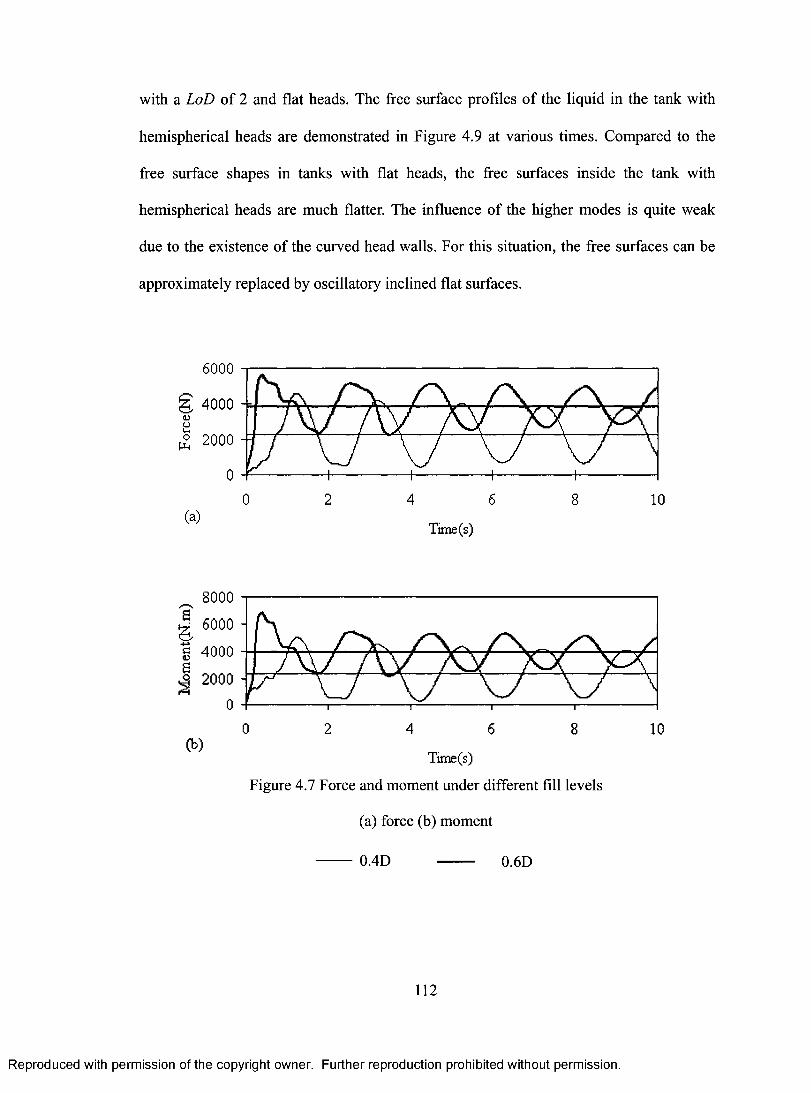
with a LoD of 2 and flat heads. The free surface profiles of the liquid in the tank with
hemispherical heads are demonstrated in Figure 4.9 at various times. Compared to the
free surface shapes in tanks with flat heads, the free surfaces inside the tank with
hemispherical heads are much flatter. The influence of the higher modes is quite weak
due to the existence of the curved head walls. For this situation, the free surfaces can be
approximately replaced by oscillatory inclined flat surfaces.
6000
g 4000
° 2000
0
(a)
8000
6000
40 4000
2000
0
0 2 4 6
Time(s)
8 10
0 2 4 6 (b)
Time(s)
Figure 4.7 Force and moment under different fill levels
(a) force (b) moment
0.4D 0.6D
112
8 10
Reproduced with permission of the copyright owner. Further reproduction prohibited without permission.
with a LoD o f 2 and flat heads. The free surface profiles o f the liquid in the tank with
hemispherical heads are demonstrated in Figure 4.9 at various times. Compared to the
free surface shapes in tanks with flat heads, the free surfaces inside the tank with
hemispherical heads are much flatter. The influence o f the higher modes is quite weak
due to the existence of the curved head walls. For this situation, the free surfaces can be
approximately replaced by oscillatory inclined flat surfaces.
6000
g, 4000<DO° 2000
0 2 4 6 8 10
Time(s)
8000
; 6000
£ 4000
S 2000
2 4 6 8 100
Time(s)
Figure 4.7 Force and moment under different fill levels
(a) force (b) moment
0.4D 0.6D
112
Reproduced with permission of the copyright owner. Further reproduction prohibited without permission.
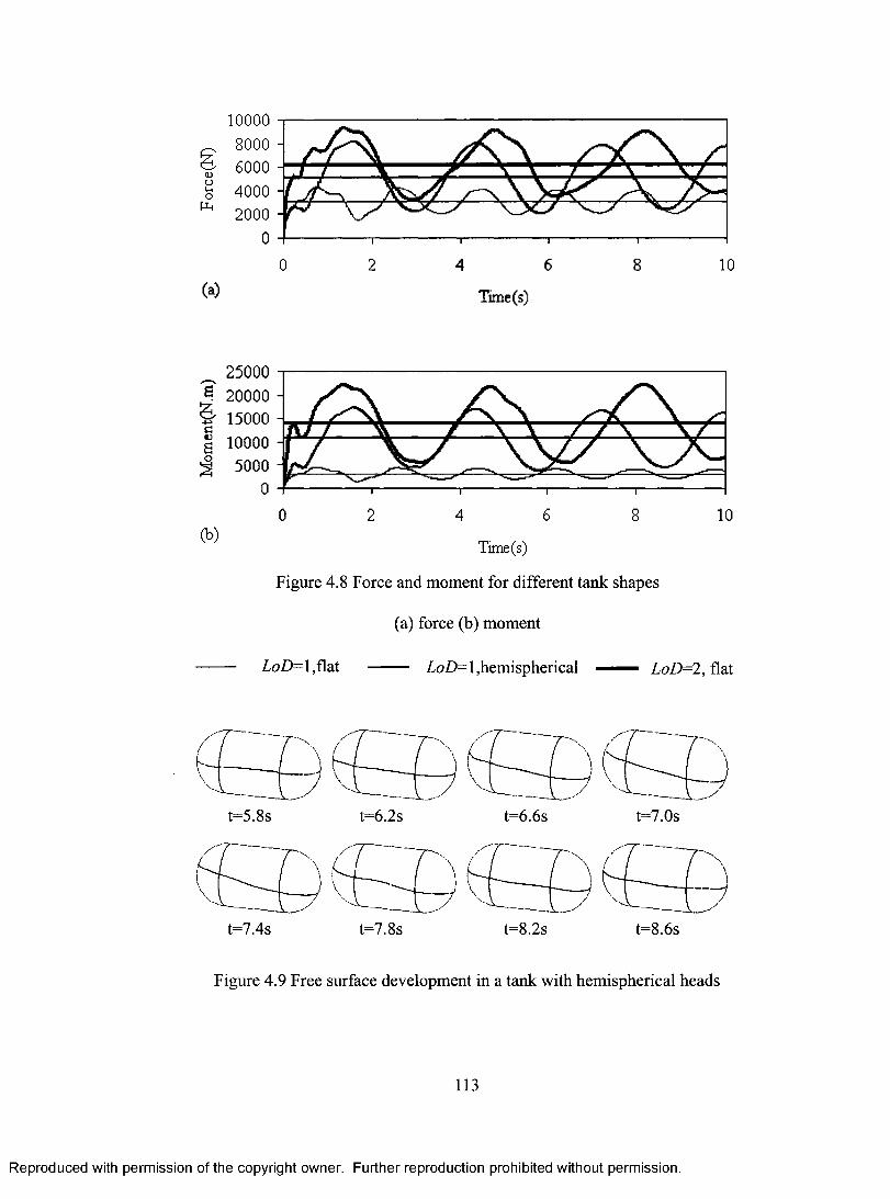
10000
a ., 8000 - 6000
,‘5° 4000 -w
2000
0
0
(a)
25000 r. 20000 15000
g 10000 5000
0
0 (b)
LoD=1,flat
t=7.4s
2 4 6
Time(s)
8 10
2 4 6
Time(s)
Figure 4.8 Force and moment for different tank shapes
(a) force (b) moment
LoD=1,hemi spherical LoD=2, flat
t=7.8s t=8.2s
8
t=8.6s
10
Figure 4.9 Free surface development in a tank with hemispherical heads
113
Reproduced with permission of the copyright owner. Further reproduction prohibited without permission.
100008000600040002000
<DO
0 2 4 6 8 10(a) Time(s)
_ 25000J 20000
15000 10000
% 5000
Cb)
0
0 8 102 4 6
Time(s)
Figure 4.8 Force and moment for different tank shapes
(a) force (b) moment
LoD= l,flat - LoD= 1 hemispherical — — LoD=2, flat
r
t=5.8s t=6.2s t=6.6s t=7.0s
t=7.4s t=7.8s t=8.2s t=8.6s
Figure 4.9 Free surface development in a tank with hemispherical heads
113
Reproduced with permission of the copyright owner. Further reproduction prohibited without permission.
The mobility of liquid cargo causes different dynamic vehicle behaviour from that
of rigid cargo, and poses challenges to researchers and engineers in vehicle stability
analysis and structure design. When the tank is subjected to a suddenly applied
acceleration, the oscillatory liquid motion causes oscillatory forces and moments of
considerable magnitudes, as shown in the above analysis and corresponding figures.
Compared to rigid cargo vehicles, the induced oscillatory forces and moments have
harmful influence on vehicle stability and controllability. They also exert cyclical
loadings on the supporting structures, which is one of the main reasons for the reduction
of the fatigue life of tank vehicle structures. It can be clearly seen from the previous
discussion that the mass centre model only shows the mean values of the oscillatory
forces and moments. It completely ignores the dynamic behaviour of the liquid and
cannot be used to describe the transient liquid motion during accelerating/braking
operations.
Numerical simulation is also conducted to study the influence of the time used for
applying the acceleration. In this case, the time is expressed by a ramp function. The
acceleration builds up to its final steady value within 4 seconds. It can be found from
Figure 4.11 that the force and moment also take the form of a ramp function and oscillate
around their equilibrium positions. At the same time, the amplitudes of the oscillations
are much smaller than those of a sudden applied acceleration. After the acceleration
reaches its steady value, the oscillation is so small that it can be neglected. Therefore,
when the acceleration is smoothly applied within a long enough time, the liquid can be
finally simplified as a rigid body by only considering the first liquid mode without
oscillation, i.e., fixed inclined flat surface. The load shift may then be obtained by using
114
Reproduced with permission of the copyright owner. Further reproduction prohibited without permission.
The mobility of liquid cargo causes different dynamic vehicle behaviour from that
o f rigid cargo, and poses challenges to researchers and engineers in vehicle stability
analysis and structure design. When the tank is subjected to a suddenly applied
acceleration, the oscillatory liquid motion causes oscillatory forces and moments of
considerable magnitudes, as shown in the above analysis and corresponding figures.
Compared to rigid cargo vehicles, the induced oscillatory forces and moments have
harmful influence on vehicle stability and controllability. They also exert cyclical
loadings on the supporting structures, which is one o f the main reasons for the reduction
o f the fatigue life o f tank vehicle structures. It can be clearly seen from the previous
discussion that the mass centre model only shows the mean values o f the oscillatory
forces and moments. It completely ignores the dynamic behaviour o f the liquid and
cannot be used to describe the transient liquid motion during accelerating/braking
operations.
Numerical simulation is also conducted to study the influence o f the time used for
applying the acceleration. In this case, the time is expressed by a ramp function. The
acceleration builds up to its final steady value within 4 seconds. It can be found from
Figure 4.11 that the force and moment also take the form of a ramp function and oscillate
around their equilibrium positions. At the same time, the amplitudes o f the oscillations
are much smaller than those of a sudden applied acceleration. After the acceleration
reaches its steady value, the oscillation is so small that it can be neglected. Therefore,
when the acceleration is smoothly applied within a long enough time, the liquid can be
finally simplified as a rigid body by only considering the first liquid mode without
oscillation, i.e., fixed inclined flat surface. The load shift may then be obtained by using
114
Reproduced with permission of the copyright owner. Further reproduction prohibited without permission.
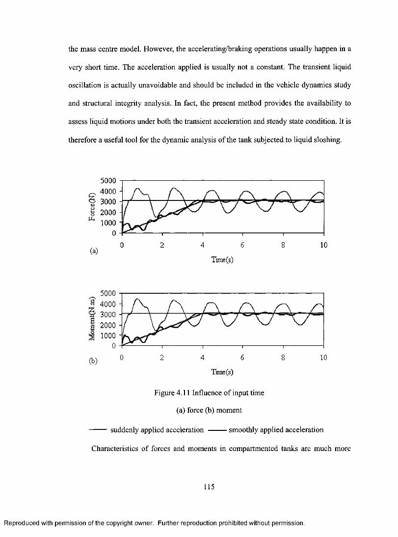
the mass centre model. However, the accelerating/braking operations usually happen in a
very short time. The acceleration applied is usually not a constant. The transient liquid
oscillation is actually unavoidable and should be included in the vehicle dynamics study
and structural integrity analysis. In fact, the present method provides the availability to
assess liquid motions under both the transient acceleration and steady state condition. It is
therefore a useful tool for the dynamic analysis of the tank subjected to liquid sloshing.
5000
a ., 4000 6 3000
O"- 2000 1-1-1
1000 0
0 (a)
5000
4000 3000
'Id 2000 1000
0
(b) 0
2 4 6
Time (s)
8 10
2 4 6
Time (s)
8 10
Figure 4.11 Influence of input time
(a) force (b) moment
suddenly applied acceleration smoothly applied acceleration
Characteristics of forces and moments in compartmented tanks are much more
115
Reproduced with permission of the copyright owner. Further reproduction prohibited without permission.
the mass centre model. However, the accelerating/braking operations usually happen in a
very short time. The acceleration applied is usually not a constant. The transient liquid
oscillation is actually unavoidable and should be included in the vehicle dynamics study
and structural integrity analysis. In fact, the present method provides the availability to
assess liquid motions under both the transient acceleration and steady state condition. It is
therefore a useful tool for the dynamic analysis of the tank subjected to liquid sloshing.
5000 _ 4000 § 3000 “ 2000
1000
uOP4
4 6 8 100 2
Time(s)
5000 4000
_ 3000 | 2000 J 1000
0 2 4 6 8 10
Time(s)
Figure 4.11 Influence o f input time
(a) force (b) moment
suddenly applied acceleration smoothly applied acceleration
Characteristics o f forces and moments in compartmented tanks are much more
115
Reproduced with permission of the copyright owner. Further reproduction prohibited without permission.
complicated. Figure 4.10 shows the simulation of a 2-compartment tank and 3-
compartment tank. The acceleration is 0.1g. The tank configurations and liquid levels are
illustrated in Figure 4.10(a). For a tank with two identical compartments, Figure 4.10(b)
shows that the axial force has the smallest variation when the two compartments have
different fill levels, i.e., case I. When the liquid levels in the two compartments are
different, the liquid frequencies are different, as shown in Figure 4.7. The asynchronous
liquid motion helps to decrease the magnitude of the varying force when the resultant
liquid force is obtained by combining the forces in both compartments. When the two
compartments have the same liquid level, i.e., case II, the synchronicity of the liquid
motion makes the force larger than that of case I, even though the tanks have the same
volume of liquid for these two cases. It can also be found that a tank with the same
volume but without a partition, i.e., case III, has the largest force, which makes it a bad
choice for carrying liquid product. It is known that the free liquid surface motion and the
liquid impact can be more severe longitudinally than laterally if no transverse partitions
are introduced (Ibrahim et al 2001). Therefore, compartmented tanks are widely used in
road transportation industry.
For a 3-compartment tank, Figure 4.10(c) shows that the axial force has the
smallest magnitude when the three compartments are filled to different levels, i.e., case
IV. For case VI, the tank is composed of a short compartment with an LoD of 1 and a
long compartment with an LoD of 2. Although the liquid frequencies are different, the
axial force has not been depressed by the asynchronous liquid motion, because the axial
force caused by the liquid in the longer compartment dominates. It should be noted that if
the liquid forces are calculated by the mass centre model, the results would be the same
116
Reproduced with permission of the copyright owner. Further reproduction prohibited without permission.
complicated. Figure 4.10 shows the simulation o f a 2-compartment tank and 3-
compartment tank. The acceleration is O.lg. The tank configurations and liquid levels are
illustrated in Figure 4.10(a). For a tank with two identical compartments, Figure 4.10(b)
shows that the axial force has the smallest variation when the two compartments have
different fill levels, i.e., case I. When the liquid levels in the two compartments are
different, the liquid frequencies are different, as shown in Figure 4.7. The asynchronous
liquid motion helps to decrease the magnitude o f the varying force when the resultant
liquid force is obtained by combining the forces in both compartments. When the two
compartments have the same liquid level, i.e., case II, the synchronicity o f the liquid
motion makes the force larger than that o f case I, even though the tanks have the same
volume o f liquid for these two cases. It can also be found that a tank with the same
volume but without a partition, i.e., case III, has the largest force, which makes it a bad
choice for carrying liquid product. It is known that the free liquid surface motion and the
liquid impact can be more severe longitudinally than laterally if no transverse partitions
are introduced (Ibrahim et al 2001). Therefore, compartmented tanks are widely used in
road transportation industry.
For a 3-compartment tank, Figure 4.10(c) shows that the axial force has the
smallest magnitude when the three compartments are filled to different levels, i.e., case
IV. For case VI, the tank is composed o f a short compartment with an LoD o f 1 and a
long compartment with an LoD o f 2. Although the liquid frequencies are different, the
axial force has not been depressed by the asynchronous liquid motion, because the axial
force caused by the liquid in the longer compartment dominates. It should be noted that if
the liquid forces are calculated by the mass centre model, the results would be the same
116
Reproduced with permission of the copyright owner. Further reproduction prohibited without permission.
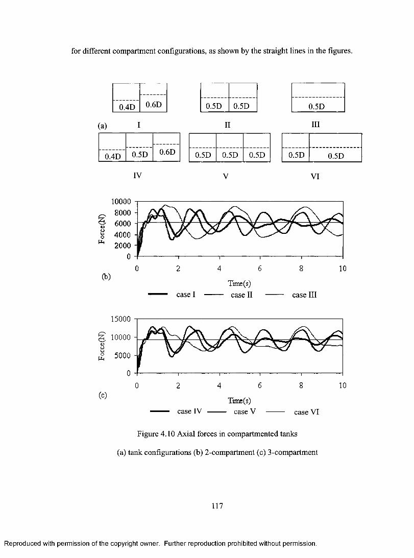
for different compartment configurations, as shown by the straight lines in the figures.
(a)
0.4D 0.6D
I
0.4D 0.5D 0.6D
10000
, .., 8000
' 6000
o'ci,
4000 P-1
2000 0
0 (b)
IV
0.5D
II
0.5D
0.5D 0.5D 0.5D
V
0.5D
III
0.5D 0.5D
VI
15000
10000 . U ,... ra-e ° 5000
(c)
0
2
case I
4 6
Time(s)
case II
8
case III
10
0 2 4 6 8
Time(s) case IV - case V case VI
Figure 4.10 Axial forces in compartmented tanks
(a) tank configurations (b) 2-compartment (c) 3-compartment
117
10
Reproduced with permission of the copyright owner. Further reproduction prohibited without permission.
for different compartment configurations, as shown by the straight lines in the figures.
0.5D 0.5D0.6D0.4D
(a) I II HI
0.6D0.4D 0.5D 0.5D 0.5D 0.5D 0.5D 0.5D
IV V VI
■DOuO[J-i
100008000600040002000
06 80 2 4 10
(b)
case ITirne(s) case II case III
Q JOU.o[J-i
(c)
15000
10000
5000
06 8 100 2 4
case IVTime(s)
■ case V case VI
Figure 4.10 Axial forces in compartmented tanks
(a) tank configurations (b) 2-compartment (c) 3-compartment
117
Reproduced with permission of the copyright owner. Further reproduction prohibited without permission.
4.5 Summary
In this chapter, a new mathematical method is developed to study the liquid
dynamics in partially filled 3D horizontal cylindrical tanks based on the method
developed for 2D circular and elliptical tanks in the previous chapter. The governing
equations based on potential flow theory, including the Laplace equation and boundary
conditions on the free surface and curved walls of a tank, are rearranged by continuous
coordinate mappings, such that the difficulties of direct discretization for numerical
calculation are avoided. The efficiency of this method has been approved by solving the
natural frequencies of a generalized eigenvalue problem using the linearized Bernoulli
equation. The transient liquid motion and corresponding liquid forces and moments
acting on the tank walls have been calculated for the tank subjected to longitudinal
acceleration input.
When the tank is subjected to a suddenly applied acceleration during
accelerating/braking operations, the liquid inside the tank undergoes severe sloshing,
which causes oscillatory forces and moments on the tank. The liquid free surface, liquid
forces, and moments under different acceleration values and liquid levels are investigated
in detail with the method developed. The influence of the existence of hemispherical
heads is studied by comparing the forces and moments to those with flat heads. The
configuration of compartmented tanks and liquid distribution inside different
compartments have a significant influence on the forces and moments, which have been
simulated and analysed under different situations for a 2-compartment tank and a 3-
compartment tank.
The methodology developed solves the transient liquid motion in a completely 3D
118
Reproduced with permission of the copyright owner. Further reproduction prohibited without permission.
4.5 Summary
In this chapter, a new mathematical method is developed to study the liquid
dynamics in partially filled 3D horizontal cylindrical tanks based on the method
developed for 2D circular and elliptical tanks in the previous chapter. The governing
equations based on potential flow theory, including the Laplace equation and boundary
conditions on the free surface and curved walls o f a tank, are rearranged by continuous
coordinate mappings, such that the difficulties o f direct discretization for numerical
calculation are avoided. The efficiency of this method has been approved by solving the
natural frequencies o f a generalized eigenvalue problem using the linearized Bernoulli
equation. The transient liquid motion and corresponding liquid forces and moments
acting on the tank walls have been calculated for the tank subjected to longitudinal
acceleration input.
When the tank is subjected to a suddenly applied acceleration during
accelerating/braking operations, the liquid inside the tank undergoes severe sloshing,
which causes oscillatory forces and moments on the tank. The liquid free surface, liquid
forces, and moments under different acceleration values and liquid levels are investigated
in detail with the method developed. The influence o f the existence o f hemispherical
heads is studied by comparing the forces and moments to those with flat heads. The
configuration o f compartmented tanks and liquid distribution inside different
compartments have a significant influence on the forces and moments, which have been
simulated and analysed under different situations for a 2-compartment tank and a 3-
compartment tank.
The methodology developed solves the transient liquid motion in a completely 3D
118
Reproduced with permission of the copyright owner. Further reproduction prohibited without permission.
manner for horizontal cylindrical tanks with flat heads and hemispherical heads. This
methodology can be used to evaluate liquid motion in tanks of arbitrarily shaped walls,
such as tanks with elliptical cross sections and tanks with other types of heads. It can also
be easily integrated into coupled liquid-structure system to study the vehicle system
dynamics. This provides the availability of a systematic analysis of the tank vehicle
structures subjected to liquid sloshing and other loadings.
119
Reproduced with permission of the copyright owner. Further reproduction prohibited without permission.
manner for horizontal cylindrical tanks with flat heads and hemispherical heads. This
methodology can be used to evaluate liquid motion in tanks o f arbitrarily shaped walls,
such as tanks with elliptical cross sections and tanks with other types o f heads. It can also
be easily integrated into coupled liquid-structure system to study the vehicle system
dynamics. This provides the availability o f a systematic analysis o f the tank vehicle
structures subjected to liquid sloshing and other loadings.
119
Reproduced with permission of the copyright owner. Further reproduction prohibited without permission.
CHAPTER 5 INFLUENCE OF LIQUID MOTION ON RIDE
QUALITY OF LIQUID CARGO TANK VEHICLES
5.1 Introduction
The issue of ride comfort is of great concern because exposure to high levels of
vibration will cause driver fatigue, which in turn can have a harmful influence on health
problems and driving safety. Ride quality problems have been studied for many years.
Some basic theories can be found in Wong (1993). A literature survey especially on heavy
vehicle ride comfort has recently been conducted by Jiang et al (2001). A general concept
of vibration-related health problems, ride comfort assessment criteria and methods and
methodology of using computer simulation to analyze ride comfort have been discussed.
Seven vehicle models, five driver/seat models, and detailed modeling techniques have
been reviewed. However, nothing has been discussed regarding ride comfort for liquid
cargo vehicles.
The ride quality of tractor semi-trailers carrying rigid cargo has attracted the
attention of several researchers in recent years (Vaduri and Law 1993, Elmadany, 1987).
However, a systematic assessment of the influence of liquid sloshing on ride quality in
partially filled tank vehicles is still outstanding in the current literature. For most tank
trucks, the total payload of the liquid cargo accounts for a large portion of the total
vehicle weight. The liquid motion within the partially filled tanks has a negative
influence on the driver's ride quality. The influence is much greater when other factors,
such as the articulation of tractor semi-trailer and B-train tank trucks, are taken into
120
Reproduced with permission of the copyright owner. Further reproduction prohibited without permission.
CHAPTER 5 INFLUENCE OF LIQUID MOTION ON RIDE
QUALITY OF LIQUID CARGO TANK VEHICLES
5.1 Introduction
The issue o f ride comfort is of great concern because exposure to high levels of
vibration will cause driver fatigue, which in turn can have a harmful influence on health
problems and driving safety. Ride quality problems have been studied for many years.
Some basic theories can be found in Wong (1993). A literature survey especially on heavy
vehicle ride comfort has recently been conducted by Jiang et al (2001). A general concept
o f vibration-related health problems, ride comfort assessment criteria and methods and
methodology o f using computer simulation to analyze ride comfort have been discussed.
Seven vehicle models, five driver/seat models, and detailed modeling techniques have
been reviewed. However, nothing has been discussed regarding ride comfort for liquid
cargo vehicles.
The ride quality of tractor semi-trailers carrying rigid cargo has attracted the
attention o f several researchers in recent years (Vaduri and Law 1993, Elmadany, 1987).
However, a systematic assessment of the influence o f liquid sloshing on ride quality in
partially filled tank vehicles is still outstanding in the current literature. For most tank
trucks, the total payload of the liquid cargo accounts for a large portion of the total
vehicle weight. The liquid motion within the partially filled tanks has a negative
influence on the driver’s ride quality. The influence is much greater when other factors,
such as the articulation of tractor semi-trailer and B-train tank trucks, are taken into
120
Reproduced with permission of the copyright owner. Further reproduction prohibited without permission.
consideration. The liquid motion depends on different operation conditions, which makes
the ride quality analysis different from that of rigid cargo vehicles.
Although the mathematical method developed in the previous chapter can be
applied to study the vehicle dynamics by integrating the fluid mechanics solution into the
vehicle system, it is basically an approach to analyzing the liquid motion in a temporal
domain, and not suitable for investigation of ride quality in a frequency domain. To study
the ride quality problem of liquid cargo vehicles, equivalent mechanical models should
be employed. In this chapter, a multi-degree-of-freedom pitch plane vehicle model
representing the dynamic response of partially filled compartmented tank vehicles is
developed and analyzed in the frequency domain to assess the effect of liquid sloshing on
ride quality. The dynamic liquid motion within the tank is modeled by a linear spring-
mass system. The input to the model is a user-specified power spectral density of the
vertical road irregularities. The power spectral density of the vertical and longitudinal
driver seat accelerations is simulated and compared with that of rigid cargo vehicles. The
influence of liquid fill level, vehicle speed, the suspension system, and road condition on
the ride quality of the tank vehicles is also investigated.
5.2 Vehicle model
The tractor semi-trailer for this study is modeled as shown in Figure 5.1. The
vehicle is considered to be traveling over an uneven road at a constant forward speed. It
is assumed that the left and right wheels of the vehicle experience identical excitations.
Vibration corresponding to the model is thus constrained to the pitch plane. The tractor
and the semi-trailer structure without payload are treated as perfect rigid bodies. The
121
Reproduced with permission of the copyright owner. Further reproduction prohibited without permission.
consideration. The liquid motion depends on different operation conditions, which makes
the ride quality analysis different from that o f rigid cargo vehicles.
Although the mathematical method developed in the previous chapter can be
applied to study the vehicle dynamics by integrating the fluid mechanics solution into the
vehicle system, it is basically an approach to analyzing the liquid motion in a temporal
domain, and not suitable for investigation o f ride quality in a frequency domain. To study
the ride quality problem of liquid cargo vehicles, equivalent mechanical models should
be employed. In this chapter, a multi-degree-of-freedom pitch plane vehicle model
representing the dynamic response of partially filled compartmented tank vehicles is
developed and analyzed in the frequency domain to assess the effect o f liquid sloshing on
ride quality. The dynamic liquid motion within the tank is modeled by a linear spring-
mass system. The input to the model is a user-specified power spectral density o f the
vertical road irregularities. The power spectral density of the vertical and longitudinal
driver seat accelerations is simulated and compared with that o f rigid cargo vehicles. The
influence o f liquid fill level, vehicle speed, the suspension system, and road condition on
the ride quality of the tank vehicles is also investigated.
5.2 Vehicle model
The tractor semi-trailer for this study is modeled as shown in Figure 5.1. The
vehicle is considered to be traveling over an uneven road at a constant forward speed. It
is assumed that the left and right wheels o f the vehicle experience identical excitations.
Vibration corresponding to the model is thus constrained to the pitch plane. The tractor
and the semi-trailer structure without payload are treated as perfect rigid bodies. The
121
Reproduced with permission of the copyright owner. Further reproduction prohibited without permission.
tractor and semi-trailer are allowed to translate in the forward and vertical directions, and
to pitch about the fifth wheel, which is modeled as a pin connection. The vehicle is
supported by three axle suspension systems. The wheels and axles are supported through
the tire springs and dampers by the road. The tires of the vehicle are assumed to remain in
contact with the road surface at all times. The seat suspension is also modeled as a linear
spring with a damper. The tank includes four compartments, as illustrated in Figure 5.1.
As verified in the previous chapter, the natural frequencies of the liquid motion in
the longitudinal direction can be effectively calculated by using an equivalent calculation
method to make use of the theory of the liquid motion response in rectangular tanks. This
equivalent method was originally established by Kobayashi et al (1989) with frequency
sweep testing. Calculated results of natural frequencies, sloshing wave heights and
sloshing forces were in good agreement with the experimental ones. Another similar
method, a summation technique, was developed by Ranganathan et al (1994) to calculate
the parameters of the spring-mass model according to the theory of sloshing response in
rectangular tanks. Although the mathematical method developed in the previous chapter
can be used in dynamic liquid motion and liquid-structure system study, it can only solve
the problems in the time domain. For the study of ride quality of the liquid cargo tank
vehicles, it is necessary to find the influence of the liquid motion on the vehicle system in
the frequency domain, and compare with the ISO standard. The equivalent mechanical
model of liquid motion, i.e., the spring-mass system, can actually be a useful tool for this
purpose. In this chapter, the equivalent method generated by Kobayashi et al (1989) is
used to study the ride quality of partially filled tank vehicles. When the liquid motion is
represented by the linear mechanical model and only the fundamental mode is
122
Reproduced with permission of the copyright owner. Further reproduction prohibited without permission.
tractor and semi-trailer are allowed to translate in the forward and vertical directions, and
to pitch about the fifth wheel, which is modeled as a pin connection. The vehicle is
supported by three axle suspension systems. The wheels and axles are supported through
the tire springs and dampers by the road. The tires of the vehicle are assumed to remain in
contact with the road surface at all times. The seat suspension is also modeled as a linear
spring with a damper. The tank includes four compartments, as illustrated in Figure 5.1.
As verified in the previous chapter, the natural frequencies o f the liquid motion in
the longitudinal direction can be effectively calculated by using an equivalent calculation
method to make use o f the theory o f the liquid motion response in rectangular tanks. This
equivalent method was originally established by Kobayashi et al (1989) with frequency
sweep testing. Calculated results o f natural frequencies, sloshing wave heights and
sloshing forces were in good agreement with the experimental ones. Another similar
method, a summation technique, was developed by Ranganathan et al (1994) to calculate
the parameters of the spring-mass model according to the theory o f sloshing response in
rectangular tanks. Although the mathematical method developed in the previous chapter
can be used in dynamic liquid motion and liquid-structure system study, it can only solve
the problems in the time domain. For the study o f ride quality o f the liquid cargo tank
vehicles, it is necessary to find the influence of the liquid motion on the vehicle system in
the frequency domain, and compare with the ISO standard. The equivalent mechanical
model of liquid motion, i.e., the spring-mass system, can actually be a useful tool for this
purpose. In this chapter, the equivalent method generated by Kobayashi et al (1989) is
used to study the ride quality of partially filled tank vehicles. When the liquid motion is
represented by the linear mechanical model and only the fundamental mode is
122
Reproduced with permission of the copyright owner. Further reproduction prohibited without permission.
considered, the liquid can be divided into two parts. One part is fixed to the tank and
moves as a rigid mass, while the other part moves as a point mass.
The displacements of the component of the vehicle system are denoted by the
independent generalized coordinates Yrp measured from the position of static equilibrium.
Yrp = [zs Zrl 191 Zil 1 ;12 Zt21 0 2 Xri • • • Xe, • • 1T (5.1)
Other dependent generalized coordinates, xs , xr2 , zr2 , x111 , .X,12 , x, 21 and ze, , are
determined by the rigid body motions, as indicated in the Figure 5.1. The dimensions of
the model are also shown in Figure 5.1. The descriptions of the generalized coordinates
are listed in Table 5.1. The masses and moments of inertia of the vehicle components,
together with the spring and damping components, will be discussed later.
The artificial soft spring and damper ( kf and cf ) attached to the tractor restrain
the otherwise semi-definite system and represent the behaviour of free rolling tires of a
vehicle traveling at a constant forward speed on a straight road. The parameters of the
spring-mass model of the liquid motion, along with the mass and moment of inertia of the
fixed part can be calculated from the equations given by Abramson and Silverman
(1966).
123
Reproduced with permission of the copyright owner. Further reproduction prohibited without permission.
considered, the liquid can be divided into two parts. One part is fixed to the tank and
moves as a rigid mass, while the other part moves as a point mass.
The displacements o f the component o f the vehicle system are denoted by the
independent generalized coordinates Yrp measured from the position o f static equilibrium.
Y r p ~ Z r \ Z l l l Z t l 2 Z t 2 \ @ 2 X r \ X e i ” ' ] ( 5 - 1 )
Other dependent generalized coordinates, xs , x r2, z r2, xlU , xtn , xt2l and zei, are
determined by the rigid body motions, as indicated in the Figure 5.1. The dimensions of
the model are also shown in Figure 5.1. The descriptions of the generalized coordinates
are listed in Table 5.1. The masses and moments o f inertia o f the vehicle components,
together with the spring and damping components, will be discussed later.
The artificial soft spring and damper ( k f and cf ) attached to the tractor restrain
the otherwise semi-definite system and represent the behaviour o f free rolling tires o f a
vehicle traveling at a constant forward speed on a straight road. The parameters o f the
spring-mass model of the liquid motion, along with the mass and moment o f inertia o f the
fixed part can be calculated from the equations given by Abramson and Silverman
(1966).
123
Reproduced with permission of the copyright owner. Further reproduction prohibited without permission.
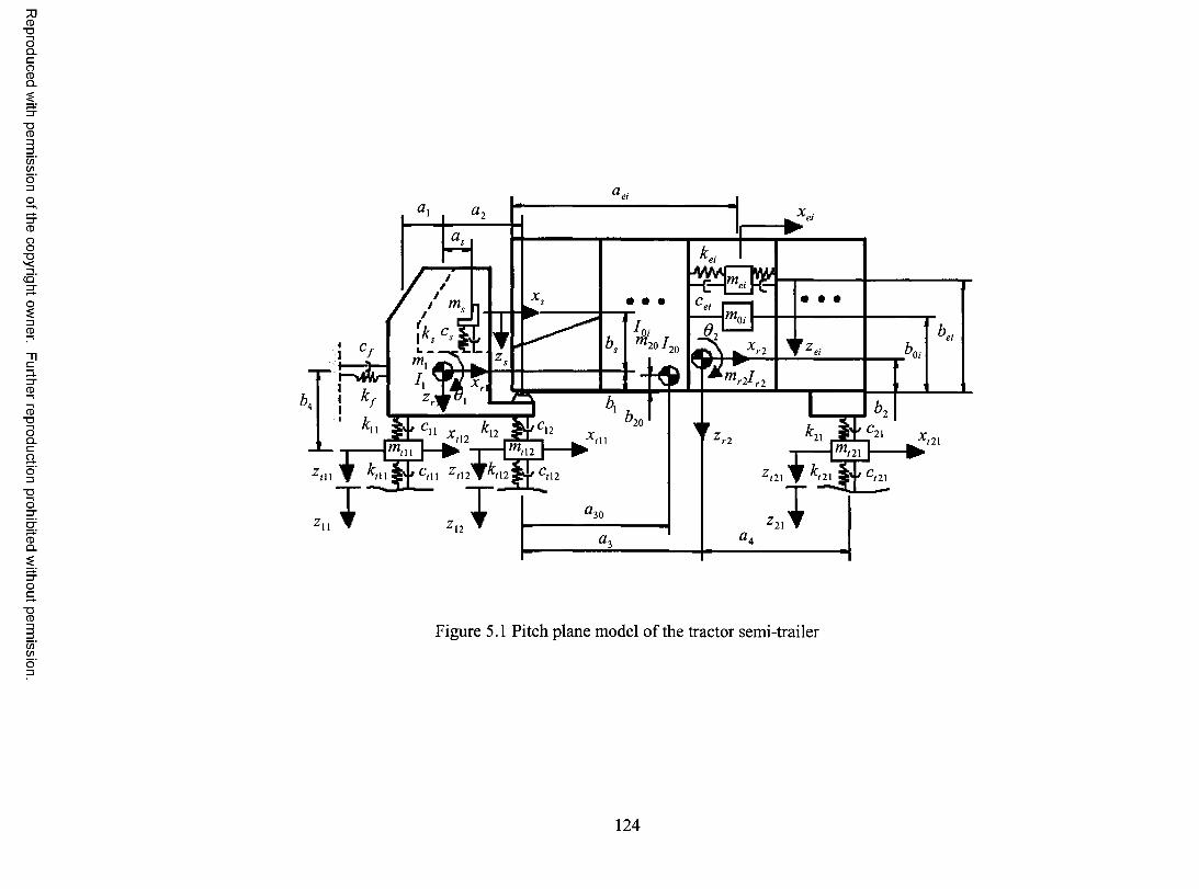
Reproduced w
ith permission o
f the copyright owner.
Further reproduction prohibited w
ithout permission.
zrll
z11
I Cf.
k11
aeia2
r
ms
i ks c L _
mi
• • •
/ 0i m 20 / 20
I 1zr 1
Cei
1121P mor
Xr ei
r 2I r2
1
mr11
b
k 12 C12 Xr12 Xrll m 12
Cri1 Zi12 r12 Cr12
Z12
a30
2
a3 a4
b2
C21 21 Xr21 m 21
Z121 Kr 21 Cr21
Figure 5.1 Pitch plane model of the tractor semi-trailer
124
Reproduced w
ith permission of the copyright ow
ner. F
urther reproduction prohibited without perm
ission.
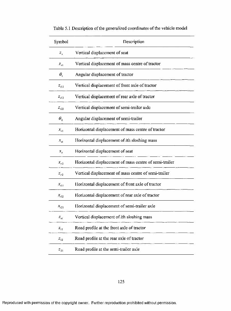
Table 5.1 Description of the generalized coordinates of the vehicle model
Symbol Description
zs Vertical displacement of seat
Zrl Vertical displacement of mass centre of tractor
Angular displacement of tractor
Znn 1 Vertical displacement of front axle of tractor
ZI12 Vertical displacement of rear axle of tractor
Zt21 Vertical displacement of semi-trailer axle
0 2 Angular displacement of semi-trailer
Xrl Horizontal displacement of mass centre of tractor
x ei Horizontal displacement of ith sloshing mass
xs Horizontal displacement of seat
Xr2 Horizontal displacement of mass centre of semi-trailer
Zr2 Vertical displacement of mass centre of semi-trailer
Horizontal displacement of front axle of tractor
x,12 Horizontal displacement of rear axle of tractor
Horizontal displacement of semi-trailer axle
Zei Vertical displacement of ith sloshing mass
Z11 Road profile at the front axle of tractor
Z12 Road profile at the rear axle of tractor
Z21 Road profile at the semi-trailer axle
125
Reproduced with permission of the copyright owner. Further reproduction prohibited without permission.
Table 5.1 Description of the generalized coordinates o f the vehicle model
Symbol Description
Vertical displacement of seat
Vertical displacement of mass centre of tractor
Angular displacement o f tractor
z m Vertical displacement o f front axle o f tractor
Z t \ 2 Vertical displacement of rear axle o f tractor
Z t 2 \ Vertical displacement o f semi-trailer axle
e2 Angular displacement o f semi-trailer
X r X Horizontal displacement o f mass centre of tractor
X e i Horizontal displacement of z'th sloshing mass
X s Horizontal displacement of seat
X r 2 Horizontal displacement o f mass centre of semi-trailer
Z r 2 Vertical displacement o f mass centre o f semi-trailer
XI\\ Horizontal displacement o f front axle of tractor
X t \ 2 Horizontal displacement of rear axle o f tractor
X t 2 1 Horizontal displacement o f semi-trailer axle
2 el Vertical displacement o f z'th sloshing mass
z xx Road profile at the front axle of tractor
Z X 2 Road profile at the rear axle o f tractor
Z 2 X Road profile at the semi-trailer axle
125
Reproduced with permission of the copyright owner. Further reproduction prohibited without permission.
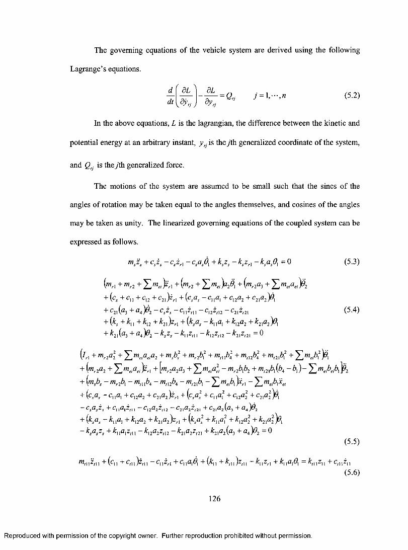
The governing equations of the vehicle system are derived using the following
Lagrange's equations.
d a a - = Q, j =1,•••,n (5.2) dt - a Y rj
In the above equations, L is the lagrangian, the difference between the kinetic and
potential energy at an arbitrary instant, yrj is the jth generalized coordinate of the system,
and Q, is the jth generalized force.
The motions of the system are assumed to be small such that the sines of the
angles of rotation may be taken equal to the angles themselves, and cosines of the angles
may be taken as unity. The linearized governing equations of the coupled system can be
expressed as follows.
msEs +csi s —cs2r,—csase9,+kszs —kszri —ksasOl = 0 (5.3)
(mri mr2 E me, )ri (mr2 E me, )a 2 5.11 (mr2a3 E meiae,
+ (Cs + CI C12 ± C21 )i ri (csas — la, + c12a2 e2ia2 + c2, (a3 + ajd2 — cs±, — c11±111—c12±112—C21-2t21
k 2i )Zri (ksas — la, + ki2a2 + k2ia2
+ k2i (a3 + a4 )02 — ksz, k2,z,21 = 0
mr2a2 E meiaeia2 msbs2 mr2bi2 + mil IN + mti2N m121b12 + E meib,2
(5.4)
±(mr2a2+ E meiaei [Mr2a2a3 E meicie2, — mr2bib2 — 4)— Im„beib,182
(msbs — mr — mi. ikt — mt. 2b4 — mt2ibi — E /17,4 )1 r1 — ineib lkq
+(csas — + c12a2 + c2,a2 + (csas2 +clog; cuai c2iaZ )41 — csasi s Cl2a 2±t12 c21a2E,21 c2ia2(a3 a4
+ ki2a2 + k2ia2 )zr, + (ksas2 + ki k21ai )91 — ksaszs + kllaizti — k12a2; 12 — k21(22zt21 + k21a2(a3 + a4 = 0
(5.5)
mmE111 (c11 cti 1a1191 (k11 km )zti = kll1z11 +ct11 11 (5.6)
126
Reproduced with permission of the copyright owner. Further reproduction prohibited without permission.
The governing equations of the vehicle system are derived using the following
Lagrange’s equations.
d_dt dy v J rJ y
81 =Qri J = l - , n (5.2)dy,
In the above equations, L is the lagrangian, the difference between the kinetic and
potential energy at an arbitrary instant, y . is the yth generalized coordinate o f the system,
and Qrj is theyth generalized force.
The motions of the system are assumed to be small such that the sines of the
angles o f rotation may be taken equal to the angles themselves, and cosines of the angles
may be taken as unity. The linearized governing equations o f the coupled system can be
expressed as follows.
m z + c z - c z , - c a d , + k z — k z , —k a 0 , = 0 (5.3)s s s s s r 1 5 s i s s s r 1 s s 1 V /
(mrt + mr2 + X ^ e iK l + ( m r 2 + + ( m r 2 a 3 +
+ ( c s + c xx + c n + c 2 i K i + ( C A - c xxa x + c n a 2 + c 2 xa ^ x
+ c2i(u3 + aA)d2 - c szs — cxxznx — cl2zt 12 — c2lzl2l (5.4)+ (K + k\ i + k]2 + klx )zrX + (ksas - kx xax + kx2a2 + k2]a2)0X + k2X{a2 + a4)02 — kszs — kxxztxx — kx2ztX2 — k2xzt2x = 0
[lri + mr2a\ + + ™A2 + mrlbx + mtX xb\ + mtnb] + mt2xbx )&x
+ ( " L 2 « 2 + + Y , m e i a l ~ m r 2 h x h + “ b X ) ~ Z m e P e P x
+ (msb, - mr2bt - mtXXb4 - m,12Z>4 - m(21Z>, - J X a K i " 2 X A * e/
+ (<A - c„fl, + c12a2 + c21a2)zrl + ( c ^ 2 + cna 2 + c12u2 + c21a22)0,
~ C s a s ^ s C \ \ a \ Z l \ \ ~ ~ C X 2 a 2 ^ l X 2 ~ ^ 2 \ a 2 Z l 2 X “*“ ^ 4 ) ^ 2
+ (* A - A + k n a 2 + k 2Xa 2 ) z rX + ( k s a ] + A:nu,2 + £12a 2 + k 2Xa 22 ] d x
- K a s z s + k xxa xz n x - k x2 a 2 z m ~ k 2 xa 2 z m + M 2 f a + a 4 ) 0 2 = 0(5.5)
m,xxzax +(cn +ctXX)ztXX - c xxzrl +cxxax0x +(kxx + klXX)ztXX - k xxzrX +kxxaxOx = knxzxx +ctxxzx(5.6)
126
Reproduced with permission of the copyright owner. Further reproduction prohibited without permission.
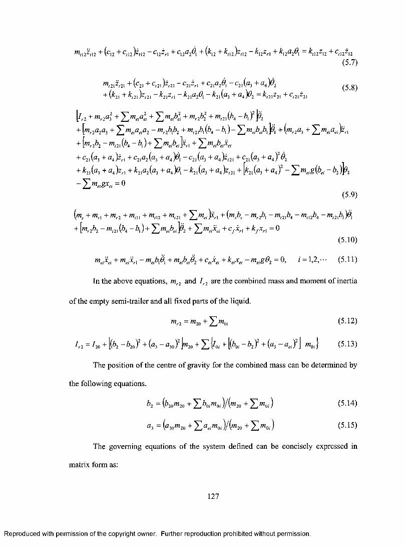
Mtl 2 t12 + ( C.12 + c 112 )±tI2 Cl2 r1 C12a 2° 1 ( k 12 k tI2 ) Zt12 k 12Zr1 k 12a 2e 1 = k tI2Z12 c tI2 12
(5.7)
m t21 t21 ( c 21 ± )t 21 — C2I i rl c n a ze i c 2I +6 /4 ) 4.92
( k 2I kt21);21 2k i Zri k 2ia 20 1 k 2 (a 3 + a.4 )0-
L = k t21 Z 21 c a1i 21
I./r2 m r2a 3 mejae2i E meibe2, m r2b m t2I ( b 4 — b l ) 212
[mr2a2a3 meiaeia2 — mr2b1b2 + mi214(b4 — b1 )— E (mr2a3 +E 1;iaei)1
+{mr2b2 — ma1(b4 — b1)+ E rrzeibei liri +Im eibeik i
c21(23 ± a 4 ) /-1 c2Ia2(a3 + a4)0, — c2i(a3 + a ) 4 ' j ai ± C21(23 4- '24 ) 262
+ k 2, (a 3 + ri k 21a 2(a 3 + a 4 ) , — k 2, (a 3 + ); 21 + [k21(a 3 +a 4 — meig(bei—Imeigxei = 0
(5.8)
2)192
(5.9)
(Ms + Mrl Mr2 Mtl I ± Mt12 ± Mt 21 ± E ( Msb s Mr2b 1 Mt2lb 4 Mil2b 4 maibiA kr2b 2 m t 21 (b4 b1)+ E meibei F 2 4- E Meii ei C f .xri k f Xri = 0
(5.10)
meibei + ineAl —meiblel+ meibeio2 + ei + keixei — meig02 = 0, i = 1,2,• • • (5.11)
In the above equations, m r2 and / r2 are the combined mass and moment of inertia
of the empty semi -trailer and all fixed parts of the liquid.
mr2 = m zo E moi
11.2 =' 20 + {(b2 b 20 + (a3 a 30 in2o E fro, + [(b0, — b2 + (a 3 — a,,) 2
(5.12)
m o,} (5.13)
The position of the centre of gravity for the combined mass can be determined by
the following equations.
b z = (b zom zo +yboimoi)/(m2.± E m 01 )
a 3 = ( a 30 m 20 E aeimoi )A m 20 E mOi
(5.14)
(5.15)
The governing equations of the system defined can be concisely expressed in
matrix form as:
127
Reproduced with permission of the copyright owner. Further reproduction prohibited without permission.
m t\2 Zt\2 + i C\2 + Cn2Xl2 C\2^r\ + c \2a 2@\ + ( 12 + 12 ) rl2 ^ \2 Z r\ + k \2 ° 2 ^ \ k t\2Z \2 + Ct\2Z \2
(5.7)
W (2 1 ^ ( 2 1 + ( C 21 + C l 2 l ) Z t 2 1 ~ C 2 \ Z r \ + C 2 \ a 2 ^ \ ~ C 2 l ( f l 3 + f l 4 ) ^ 2 ^ g ^
+ ( & 21 ^ k l 2 i ) z , 2 i ~ k 2 \ Z r \ — k l x a 2 O x — k 2 \ i . a 2 + ^ 4 ) ^ 2 — ^ 7 2 \ Z 2 \ ^ C t 2 \ Z 2 \
[7,2 + m n a \ + Y j m eia l i + Y j m e.b l + m r2b 2 + ™ t2 \ ib 4 “ b \ f J 2
Wr2a2fl3 + T j m eia eia 2 ~ m r2b A + *”,21^4 “ A)" Z ™«AA]^1 + (Wr2«3 + Z W*fl*K l
m r2b 2 ~ m m ( b 4 - A) + Z ™ A f c l + Z ™ A A
C 21 ( ^ 3 ^ 4 ) ^ r l C 2 1 ^ 2 ( f l 3 ^ 4 ) ^ 1 _ C 2 I ( ^ 3 ^ 4 ) ^ / 2 l C 21 ( f l 3 ^ 4 ) ^ 2
+ £21(a3 + a4)zH + £ 21a2(a3 + a4)6> - * 2 i ( « 3 + a 4 ) z m + [*2i(«3 + o 4)2 - Z w«-gfe/ A ) k
- Z WrfS*e*=°(5.9)
k + Wr, + ror2 + /»„, + mn2 + mt2l + £ mei)xrl + (msbs - mr2bx - mt2lb4 - mn2b4 - ml2xbx )0X
+ [™r2b 2 - m ,2 \{b 4 ~ b l ) + Z W A & + Z V e i + C f K \ + k f X r\ = 0
( 5 . 1 0 )
m elX a + m j r l ~ m eib A + m c A A + C eiK i + K i* e i ~ ™ e iS d 2 = 0> * = A V •1 1)
In the above equations, mr2 and I r2 are the combined mass and moment o f inertia
of the empty semi-trailer and all fixed parts o f the liquid.
m r2 = m 20 + Z m 0i (5-12)
7,2 =ho+[(b2 - b2of +(a3 - a2o)2\ n20 + T J^Oi + [(bOi-b2 f + (a2 - aei)2\ m0i] (5-13)
The position o f the centre o f gravity for the combined mass can be determined by
the following equations.
b 2 = (h io W io + Z 60,™0, )/ko + Z OTo/) (5-14)
« 3 = ( « 3 0 W 20 + Z ^ - m 0 1 ) / k o + Z ' ” 0i ) ( 5 ‘ 1 5 )
The governing equations o f the system defined can be concisely expressed in
matrix form as:
127
Reproduced with permission of the copyright owner. Further reproduction prohibited without permission.
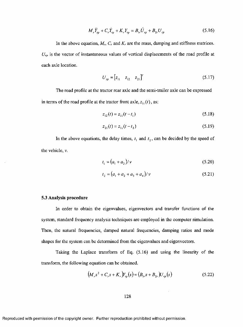
M r f rp ± C r icp ± K r Yrp = B ir L I rp ± B 2rU rp (5.16)
In the above equation, Mr, Cr and Kr are the mass, damping and stiffness matrices.
Urp is the vector of instantaneous values of vertical displacements of the road profile at
each axle location.
211T U rp = Z[z11 z 12 (5.17)
The road profile at the tractor rear axle and the semi-trailer axle can be expressed
in terms of the road profile at the tractor front axle, z,1(t), as:
Z12 ( t ) = Z I1 ( t — t l ) (5.18)
z21(t) = zii(t — t2) (5.19)
In the above equations, the delay times, t, and t2 , can be decided by the speed of
the vehicle, v.
t, = (a, +a2 )/v (5.20)
t2 = (a, + a2 + a3 + a4 )/v (5.21)
5.3 Analysis procedure
In order to obtain the eigenvalues, eigenvectors and transfer functions of the
system, standard frequency analysis techniques are employed in the computer simulation.
Then, the natural frequencies, damped natural frequencies, damping ratios and mode
shapes for the system can be determined from the eigenvalues and eigenvectors.
Taking the Laplace transform of Eq. (5.16) and using the linearity of the
transform, the following equation can be obtained.
(Mrs 2 + C rS + Kr )Y,p(s)= (Ars + B 2r )U rp (S) (5.22)
128
Reproduced with permission of the copyright owner. Further reproduction prohibited without permission.
M X P +CrYrp + K J rp= B [rUrp+B2rUrp (5.16)
In the above equation, Mr, Cr and Kr are the mass, damping and stiffness matrices.
Urp is the vector of instantaneous values of vertical displacements o f the road profile at
each axle location.
Urp=[zu z l2 z 2J (5.17)
The road profile at the tractor rear axle and the semi-trailer axle can be expressed
in terms o f the road profile at the tractor front axle, z ,, ( t ) , as:
z i2(t) = z n (* -* ,) (5.18)
z 2\(t) = z u ( t - t 2) (5.19)
In the above equations, the delay times, t] and t2, can be decided by the speed of
the vehicle, v.
ty - (a, +a2) /v (5.20)
t2 = (ax + a2 + a 3 +a4) /v (5.21)
5.3 Analysis procedure
In order to obtain the eigenvalues, eigenvectors and transfer functions of the
system, standard frequency analysis techniques are employed in the computer simulation.
Then, the natural frequencies, damped natural frequencies, damping ratios and mode
shapes for the system can be determined from the eigenvalues and eigenvectors.
Taking the Laplace transform of Eq. (5.16) and using the linearity o f the
transform, the following equation can be obtained.
(hi,*1 + C rS + K X ( s ) = ( K s + Blr)Ure(s) (5-22)
128
Reproduced with permission of the copyright owner. Further reproduction prohibited without permission.
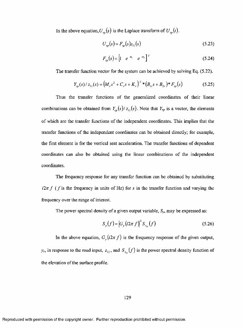
In the above equation, U rp (s) is the Laplace transform of U rp (t).
U rp (S)=-- Frp (s)zil (s) (5.23)
Frp (s)=[1 e-st' e-'21 T (5.24)
The transfer function vector for the system can be achieved by solving Eq. (5.22).
I', (s) / zl , (s) =(1 rs2 + C rs + Kr ) 1 *(1211rs+B2r )* F rp (S) (5.25)
Thus the transfer functions of the generalized coordinates of their linear
combinations can be obtained from Yrp (s)/ z11 (s). Note that Yrp is a vector, the elements
of which are the transfer functions of the independent coordinates. This implies that the
transfer functions of the independent coordinates can be obtained directly; for example,
the first element is for the vertical seat acceleration. The transfer functions of dependent
coordinates can also be obtained using the linear combinations of the independent
coordinates.
The frequency response for any transfer function can be obtained by substituting
i2z f (f is the frequency in units of Hz) for s in the transfer function and varying the
frequency over the range of interest.
The power spectral density of a given output variable, Sy, may be expressed as:
S y (f)=1G y (i2ir f)1 2 S zu (f) (5.26)
In the above equation, G y (i2rc f) is the frequency response of the given output,
yr, in response to the road input, z11 , and Szii (f) is the power spectral density function of
the elevation of the surface profile.
129
Reproduced with permission of the copyright owner. Further reproduction prohibited without permission.
In the above equation,!/ is) is the Laplace transform of Urp(t).
= / / » „ ( * ) (5-23)
Fn,(s)=[l e-'1' e - ' ^ Y (5.24)
The transfer function vector for the system can be achieved by solving Eq. (5.22).
y „ (s )/ Z|,M = { M y + C,s + AT,)'1 • (Blrs + f l j * F j s ) (5.25)
Thus the transfer functions of the generalized coordinates o f their linear
combinations can be obtained from Yrp{s)lzu (s). Note that Yv is a vector, the elements
o f which are the transfer functions o f the independent coordinates. This implies that the
transfer functions o f the independent coordinates can be obtained directly; for example,
the first element is for the vertical seat acceleration. The transfer functions o f dependent
coordinates can also be obtained using the linear combinations o f the independent
coordinates.
The frequency response for any transfer function can be obtained by substituting
i2n f ( / is the frequency in units of Hz) for s in the transfer function and varying the
frequency over the range of interest.
The power spectral density o f a given output variable, Sy, may be expressed as:
S , ( f ) = \ G y{ i 2 x f f s , a ( f ) (5.26)
In the above equation, Gy {i2n / ) is the frequency response o f the given output,
y r, in response to the road input, zn , and 5lZ i ( / ) is the power spectral density function of
the elevation o f the surface profile.
129
Reproduced with permission of the copyright owner. Further reproduction prohibited without permission.
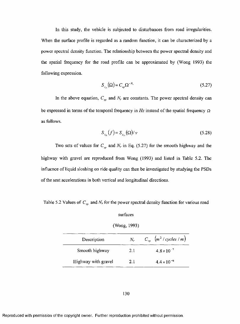
In this study, the vehicle is subjected to disturbances from road irregularities.
When the surface profile is regarded as a random function, it can be characterized by a
power spectral density function. The relationship between the power spectral density and
the spatial frequency for the road profile can be approximated by (Wong 1993) the
following expression.
szIl (ci) = c„friv, (5.27)
In the above equation, Csp and Nr are constants. The power spectral density can
be expressed in terms of the temporal frequency in Hz instead of the spatial frequency n
as follows.
S zii (f)= S z (S2)/ v (5.28)
Two sets of values for Cs/0 and Al", in Eq. (5.27) for the smooth highway and the
highway with gravel are reproduced from Wong (1993) and listed in Table 5.2. The
influence of liquid sloshing on ride quality can then be investigated by studying the PSDs
of the seat accelerations in both vertical and longitudinal directions.
Table 5.2 Values of Csp and Nr for the power spectral density function for various road
surfaces
(Wong, 1993)
Description Nr Csp (In 2 / cycles I m)
Smooth highway 2.1 4.8 x10⁻⁷
Highway with gravel 2.1 4.4 x10 -6
130
Reproduced with permission of the copyright owner. Further reproduction prohibited without permission.
In this study, the vehicle is subjected to disturbances from road irregularities.
When the surface profde is regarded as a random function, it can be characterized by a
power spectral density function. The relationship between the power spectral density and
the spatial frequency for the road profile can be approximated by (Wong 1993) the
following expression.
In the above equation, Csp and Nr are constants. The power spectral density can
be expressed in terms of the temporal frequency in Hz instead o f the spatial frequency Q
as follows.
Two sets o f values for Csp and Nr in Eq. (5.27) for the smooth highway and the
highway with gravel are reproduced from Wong (1993) and listed in Table 5.2. The
influence o f liquid sloshing on ride quality can then be investigated by studying the PSDs
o f the seat accelerations in both vertical and longitudinal directions.
Table 5.2 Values o f Csp and Nr for the power spectral density function for various road
surfaces
(5.27)
(5.28)
(Wong, 1993)
Description Nr Csp (m2 / cycles / m)
Smooth highway 2.1 4.8 x 10"7
Highway with gravel 2.1 4.4 x 10~6
130
Reproduced with permission of the copyright owner. Further reproduction prohibited without permission.
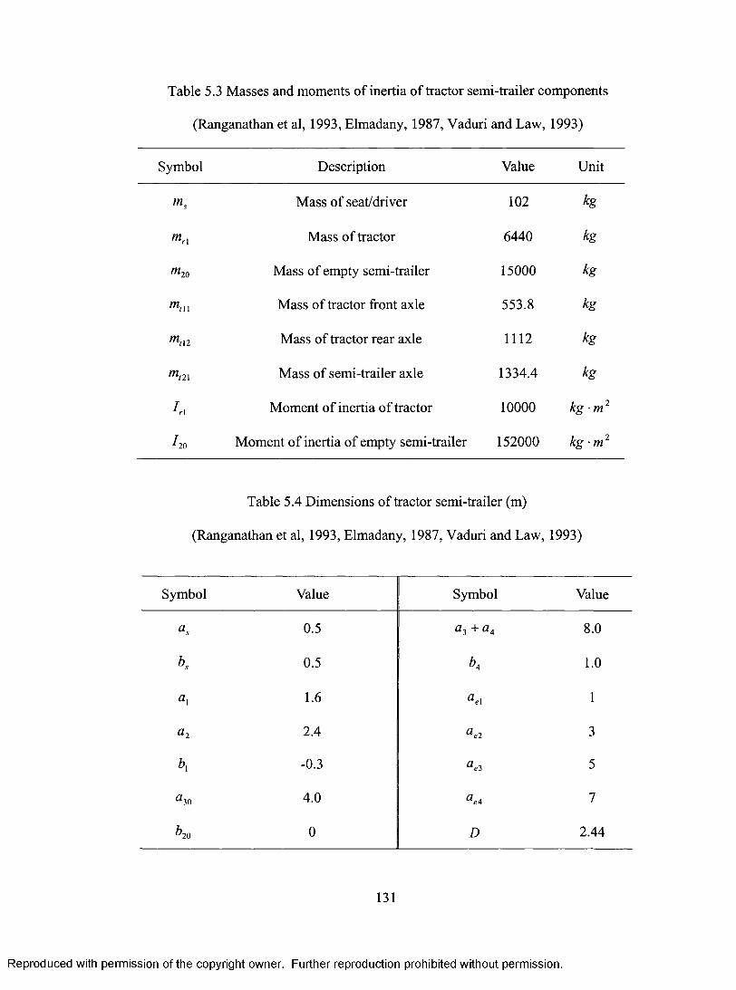
Table 5.3 Masses and moments of inertia of tractor semi-trailer components
(Ranganathan et al, 1993, Elmadany, 1987, Vaduri and Law, 1993)
Symbol Description Value Unit
Ins Mass of seat/driver 102 kg
Mel Mass of tractor 6440 kg
m20 Mass of empty semi-trailer 15000 kg
mtll Mass of tractor front axle 553.8 kg
mt12 Mass of tractor rear axle 1112 kg
mt 21 Mass of semi-trailer axle 1334.4 kg
Iri Moment of inertia of tractor 10000 kg • m 2
-120 Moment of inertia of empty semi-trailer 152000 kg • m 2
Table 5.4 Dimensions of tractor semi-trailer (m)
(Ranganathan et al, 1993, Elmadany, 1987, Vaduri and Law, 1993)
Symbol Value Symbol Value
as 0.5 a3 + a4 8.0
bs 0.5 b4 1.0
a1 1.6 a el 1
a 2 2.4 ae2 3
bt -0.3 ae3 5
a30 4.0 ae4 7
b20 0 D 2.44
131
Reproduced with permission of the copyright owner. Further reproduction prohibited without permission.
Table 5.3 Masses and moments o f inertia o f tractor semi-trailer components
(Ranganathan et al, 1993, Elmadany, 1987, Vaduri and Law, 1993)
Symbol Description Value Unit
ms Mass of seat/driver 102 kg
mrX Mass o f tractor 6440 kg
m20 Mass o f empty semi-trailer 15000 kg
mm Mass of tractor front axle 553.8 kg
mtM Mass o f tractor rear axle 1112 kg
ml2i Mass of semi-trailer axle 1334.4 kg
In Moment of inertia o f tractor 10000 kg • m
120 Moment o f inertia of empty semi-trailer 152000 kg ■ m
Table 5.4 Dimensions o f tractor semi-trailer (m)
(Ranganathan et al, 1993, Elmadany, 1987, Vaduri and Law, 1993)
Symbol Value Symbol Value
as 0.5 8.0
bs 0.5 K 1.0
1.6 ael 1
a2 2.4 ae2 3
-0.3 aei 5
aio 4.0 ae4 7
20 0 D 2.44
131
Reproduced with permission of the copyright owner. Further reproduction prohibited without permission.
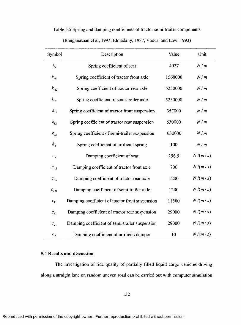
Table 5.5 Spring and damping coefficients of tractor semi-trailer components
(Ranganathan et al, 1993, Elmadany, 1987, Vaduri and Law, 1993)
Symbol Description Value Unit
k,
k tll
Spring coefficient of seat
Spring coefficient of tractor front axle
4027
1560000
N / m
N 1m
kl2 Spring coefficient of tractor rear axle 5250000 N / m
k 121 Spring coefficient of semi-trailer axle 5250000 N / m
k11 Spring coefficient of tractor front suspension 357000 N / m
ki2 Spring coefficient of tractor rear suspension 630000 N / m
k 21 Spring coefficient of semi-trailer suspension 630000 N / m
kf Spring coefficient of artificial spring 100 N / m
cs Damping coefficient of seat 256.5 N 1(m / s)
CtIl Damping coefficient of tractor front axle 700 N /(m / s)
C,12 Damping coefficient of tractor rear axle 1200 N 1(ml s)
Ct21 Damping coefficient of semi-trailer axle 1200 N 1(m / s)
C11 Damping coefficient of tractor front suspension 11500 N /(m I s)
C12 Damping coefficient of tractor rear suspension 29000 N 1(m / s)
C21 Damping coefficient of semi-trailer suspension 29000 N 1(m / s)
Cf Damping coefficient of artificial damper 10 N /(m I s)
5.4 Results and discussion
The investigation of ride quality of partially filled liquid cargo vehicles driving
along a straight lane on random uneven road can be carried out with computer simulation
132
Reproduced with permission of the copyright owner. Further reproduction prohibited without permission.
Table 5.5 Spring and damping coefficients o f tractor semi-trailer components
(Ranganathan et al, 1993, Elmadany, 1987, Vaduri and Law, 1993)
Symbol Description Value Unit
K Spring coefficient o f seat 4027 N / m
K n Spring coefficient of tractor front axle 1560000 N tm
K n Spring coefficient o f tractor rear axle 5250000 N / m
kt2\ Spring coefficient of semi-trailer axle 5250000 N / m
kn Spring coefficient o f tractor front suspension 357000 N / m
k\2 Spring coefficient o f tractor rear suspension 630000 N / m
k2l Spring coefficient o f semi-trailer suspension 630000 N / m
k f Spring coefficient of artificial spring 100 N / m
cs Damping coefficient o f seat 256.5 N /(m / s )
cm Damping coefficient o f tractor front axle 700 N /(m/ s)
Ct\2 Damping coefficient o f tractor rear axle 1200 N /(m l s)
Ct2\ Damping coefficient o f semi-trailer axle 1200 N /(m / s )
Cu Damping coefficient o f tractor front suspension 11500 N /(m/ s)
cX2 Damping coefficient o f tractor rear suspension 29000 N !{m / 5 )
C 2l Damping coefficient of semi-trailer suspension 29000 N l(ml s)
Cf Damping coefficient of artificial damper 10 N l(ml s)
5.4 Results and discussion
The investigation of ride quality o f partially filled liquid cargo vehicles driving
along a straight lane on random uneven road can be carried out with computer simulation
132
Reproduced with permission of the copyright owner. Further reproduction prohibited without permission.
employing the power spectral density of the driver seat accelerations in both vertical and
horizontal directions. The PSDs are determined by substituting the different frequency
values (in the calculation, 200 points from 0.1 Hz to 100 Hz are used) directly into the
expressions of the desired functions, such as the vertical and horizontal accelerations,
after Eq. (5.26) is obtained.
The candidate tank includes four separated compartments. Therefore, four degrees
of freedom are needed to describe the liquid motion of the tank vehicle, and it is assumed
that the four parts of liquid in different compartments have the same fill levels. The
parameters used in the simulation are listed in Tables 5.3, 5.4 and 5.5 (Ranganathan et al,
1993, Elmadany, 1987, Vaduri and Law, 1993). The symbol D, which is not shown in
Figure 5.1, represents the diameter of the tank.
5.4.1 Frequency characteristics of partially filled liquid cargo vehicles
The natural frequencies of the vehicle system are calculated for different fill
levels under the given tank configurations. The frequencies due to the liquid sloshing
modes are in the frequency range of 0.1-0.7 Hz. Table 5.6 lists the frequencies for two
different fill levels, 30% and 70%. As shown in the table, the frequencies due to the
liquid sloshing modes increase with the increase of the liquid fill levels, while the
frequencies due to the bounce and pitch modes of the tractor and semi-trailer decrease
with the increase in the fill levels. It should be noted that when the fill level increases, the
increased mass and moment of inertia will make the frequencies of the bounce and pitch
modes of the tractor and semi-trailer lower. At the same time, the frequencies of liquid
sloshing will increase because of the higher fill level. This will generate a coupled effect
133
Reproduced with permission of the copyright owner. Further reproduction prohibited without permission.
employing the power spectral density of the driver seat accelerations in both vertical and
horizontal directions. The PSDs are determined by substituting the different frequency
values (in the calculation, 200 points from 0.1 Hz to 100 Hz are used) directly into the
expressions o f the desired functions, such as the vertical and horizontal accelerations,
after Eq. (5.26) is obtained.
The candidate tank includes four separated compartments. Therefore, four degrees
o f freedom are needed to describe the liquid motion of the tank vehicle, and it is assumed
that the four parts o f liquid in different compartments have the same fill levels. The
parameters used in the simulation are listed in Tables 5.3, 5.4 and 5.5 (Ranganathan et al,
1993, Elmadany, 1987, Vaduri and Law, 1993). The symbol D, which is not shown in
Figure 5.1, represents the diameter o f the tank.
5.4.1 Frequency characteristics of partially filled liquid cargo vehicles
The natural frequencies of the vehicle system are calculated for different fill
levels under the given tank configurations. The frequencies due to the liquid sloshing
modes are in the frequency range of 0.1-0.7 Hz. Table 5.6 lists the frequencies for two
different fill levels, 30% and 70%. As shown in the table, the frequencies due to the
liquid sloshing modes increase with the increase o f the liquid fill levels, while the
frequencies due to the bounce and pitch modes of the tractor and semi-trailer decrease
with the increase in the fill levels. It should be noted that when the fill level increases, the
increased mass and moment o f inertia will make the frequencies o f the bounce and pitch
modes of the tractor and semi-trailer lower. At the same time, the frequencies of liquid
sloshing will increase because o f the higher fill level. This will generate a coupled effect
133
Reproduced with permission of the copyright owner. Further reproduction prohibited without permission.
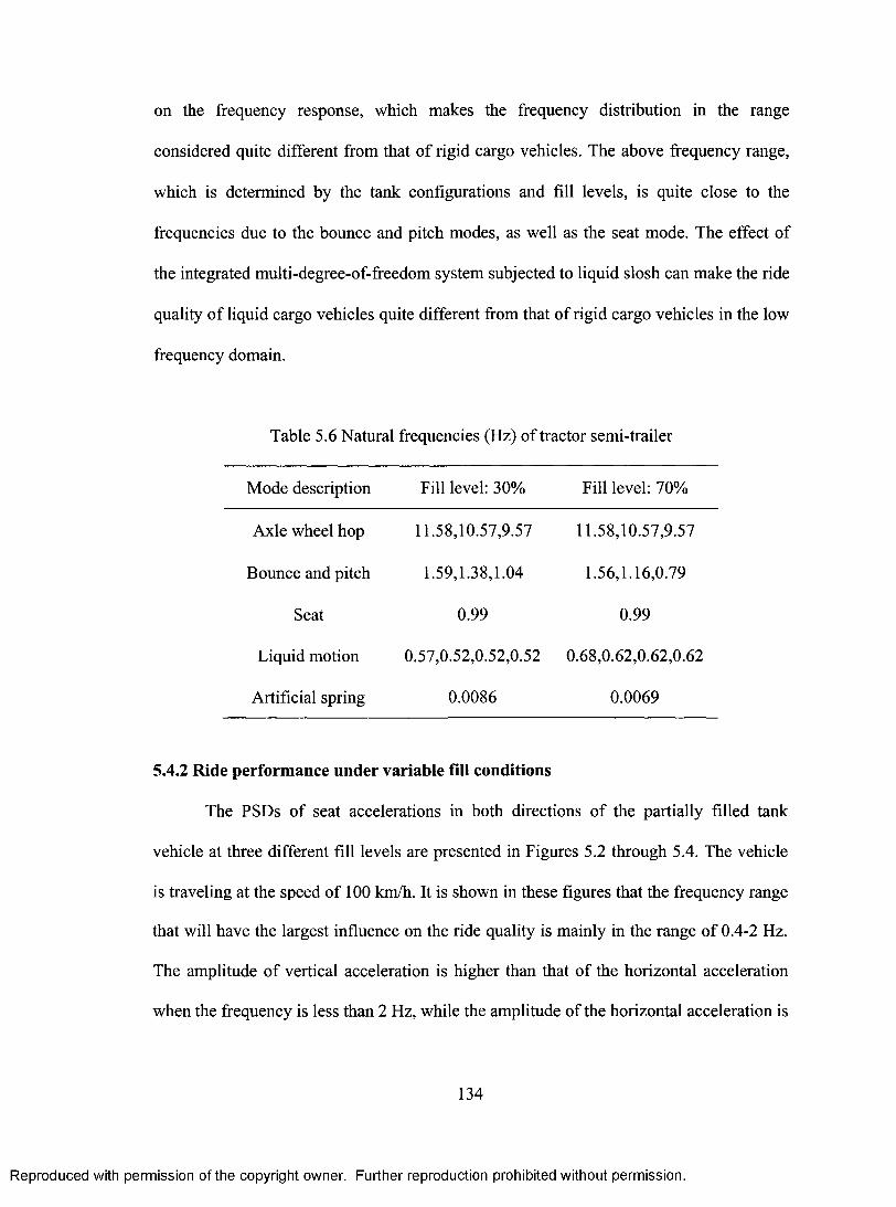
on the frequency response, which makes the frequency distribution in the range
considered quite different from that of rigid cargo vehicles. The above frequency range,
which is determined by the tank configurations and fill levels, is quite close to the
frequencies due to the bounce and pitch modes, as well as the seat mode. The effect of
the integrated multi-degree-of-freedom system subjected to liquid slosh can make the ride
quality of liquid cargo vehicles quite different from that of rigid cargo vehicles in the low
frequency domain.
Table 5.6 Natural frequencies (Hz) of tractor semi-trailer
Mode description Fill level: 30% Fill level: 70%
Axle wheel hop 11.58,10.57,9.57 11.58,10.57,9.57
Bounce and pitch 1.59,1.38,1.04 1.56,1.16,0.79
Seat 0.99 0.99
Liquid motion 0.57,0.52,0.52,0.52 0.68,0.62,0.62,0.62
Artificial spring 0.0086 0.0069
5.4.2 Ride performance under variable fill conditions
The PSDs of seat accelerations in both directions of the partially filled tank
vehicle at three different fill levels are presented in Figures 5.2 through 5.4. The vehicle
is traveling at the speed of 100 km/h. It is shown in these figures that the frequency range
that will have the largest influence on the ride quality is mainly in the range of 0.4-2 Hz.
The amplitude of vertical acceleration is higher than that of the horizontal acceleration
when the frequency is less than 2 Hz, while the amplitude of the horizontal acceleration is
134
Reproduced with permission of the copyright owner. Further reproduction prohibited without permission.
on the frequency response, which makes the frequency distribution in the range
considered quite different from that of rigid cargo vehicles. The above frequency range,
which is determined by the tank configurations and fill levels, is quite close to the
frequencies due to the bounce and pitch modes, as well as the seat mode. The effect of
the integrated multi-degree-of-ffeedom system subjected to liquid slosh can make the ride
quality o f liquid cargo vehicles quite different from that o f rigid cargo vehicles in the low
frequency domain.
Table 5.6 Natural frequencies (Hz) o f tractor semi-trailer
Mode description Fill level: 30% Fill level: 70%
Axle wheel hop 11.58,10.57,9.57 11.58,10.57,9.57
Bounce and pitch 1.59,1.38,1.04 1.56,1.16,0.79
Seat 0.99 0.99
Liquid motion 0.57,0.52,0.52,0.52 0.68,0.62,0.62,0.62
Artificial spring 0.0086 0.0069
5.4.2 Ride performance under variable fill conditions
The PSDs o f seat accelerations in both directions o f the partially filled tank
vehicle at three different fill levels are presented in Figures 5.2 through 5.4. The vehicle
is traveling at the speed of 100 km/h. It is shown in these figures that the frequency range
that will have the largest influence on the ride quality is mainly in the range of 0.4-2 Hz.
The amplitude o f vertical acceleration is higher than that of the horizontal acceleration
when the frequency is less than 2 Hz, while the amplitude of the horizontal acceleration is
134
Reproduced with permission of the copyright owner. Further reproduction prohibited without permission.
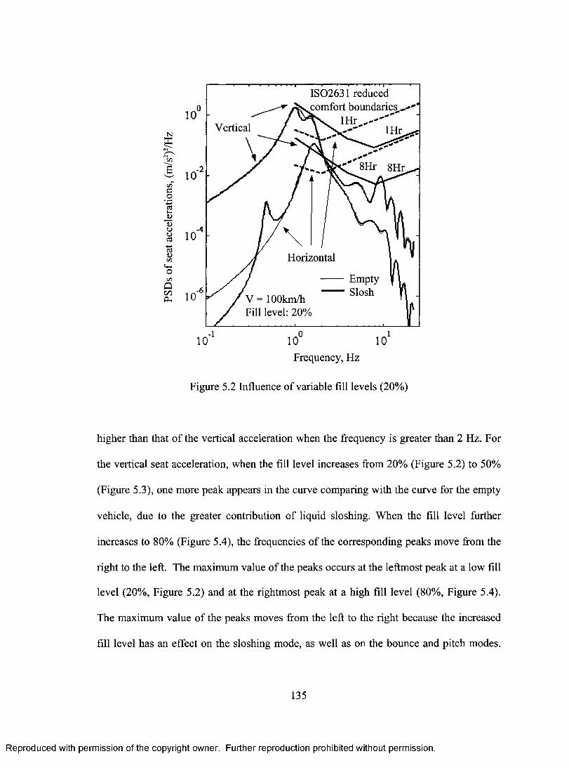
PS
Ds
of s
eat a
ccel
erat
ions
, (m
/s2)
2/H
z
100
10 2
10 4
10-6
104
Vertical ---------..
ISO2631 reduced comfort boundaries.....--' . ..
1Hr, .- ....0-1Hr
.0.
Horizontal
V = 100km/h Fill level: 20%
Empty Slosh
100
Frequency, Hz
101
Figure 5.2 Influence of variable fill levels (20%)
higher than that of the vertical acceleration when the frequency is greater than 2 Hz. For
the vertical seat acceleration, when the fill level increases from 20% (Figure 5.2) to 50%
(Figure 5.3), one more peak appears in the curve comparing with the curve for the empty
vehicle, due to the greater contribution of liquid sloshing. When the fill level further
increases to 80% (Figure 5.4), the frequencies of the corresponding peaks move from the
right to the left. The maximum value of the peaks occurs at the leftmost peak at a low fill
level (20%, Figure 5.2) and at the rightmost peak at a high fill level (80%, Figure 5.4).
The maximum value of the peaks moves from the left to the right because the increased
fill level has an effect on the sloshing mode, as well as on the bounce and pitch modes.
135
Reproduced with permission of the copyright owner. Further reproduction prohibited without permission.
Nffi
C/3Uou<L>
13ooacdd>C/3twOC/3
QooPh
IS02631 reduced comfort boundaries.,'
1 HrlH rVertical
\: 8Hr 8Hr
Horizontal
EmptySlosh
V = lOOkm/h Fill level: 20%
10 10 '
Frequency, Hz
Figure 5.2 Influence of variable fill levels (20%)
higher than that o f the vertical acceleration when the frequency is greater than 2 Hz. For
the vertical seat acceleration, when the fill level increases from 20% (Figure 5.2) to 50%
(Figure 5.3), one more peak appears in the curve comparing with the curve for the empty
vehicle, due to the greater contribution o f liquid sloshing. When the fill level further
increases to 80% (Figure 5.4), the frequencies of the corresponding peaks move from the
right to the left. The maximum value o f the peaks occurs at the leftmost peak at a low fill
level (20%, Figure 5.2) and at the rightmost peak at a high fill level (80%, Figure 5.4).
The maximum value of the peaks moves from the left to the right because the increased
fill level has an effect on the sloshing mode, as well as on the bounce and pitch modes.
135
Reproduced with permission of the copyright owner. Further reproduction prohibited without permission.
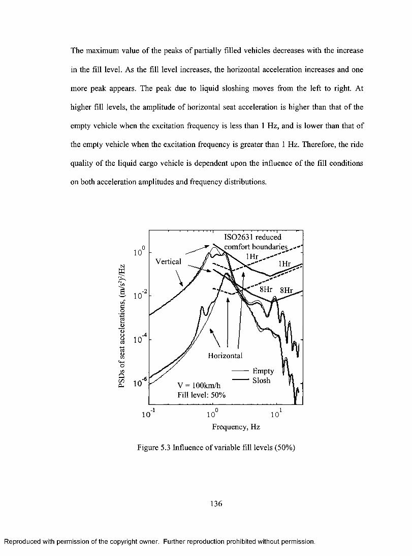
The maximum value of the peaks of partially filled vehicles decreases with the increase
in the fill level. As the fill level increases, the horizontal acceleration increases and one
more peak appears. The peak due to liquid sloshing moves from the left to right. At
higher fill levels, the amplitude of horizontal seat acceleration is higher than that of the
empty vehicle when the excitation frequency is less than 1 Hz, and is lower than that of
the empty vehicle when the excitation frequency is greater than 1 Hz. Therefore, the ride
quality of the liquid cargo vehicle is dependent upon the influence of the fill conditions
on both acceleration amplitudes and frequency distributions.
PS
Ds
of s
eat a
ccel
erat
ions
, (m
/s2)
Z/H
z
10o
10 2
10
0-6
Vertical
ISO2631 reduced comfort boundaries,,,--
1Hr .,---'1Hr
Horizontal
V = 100km/h Fill level: 50%
Empty Slosh
10-1
100
Frequency, Hz
101
Figure 5.3 Influence of variable fill levels (50%)
136
Reproduced with permission of the copyright owner. Further reproduction prohibited without permission.
The maximum value of the peaks of partially filled vehicles decreases with the increase
in the fill level. As the fill level increases, the horizontal acceleration increases and one
more peak appears. The peak due to liquid sloshing moves from the left to right. At
higher fill levels, the amplitude o f horizontal seat acceleration is higher than that of the
empty vehicle when the excitation frequency is less than 1 Hz, and is lower than that of
the empty vehicle when the excitation frequency is greater than 1 Hz. Therefore, the ride
quality o f the liquid cargo vehicle is dependent upon the influence of the fill conditions
on both acceleration amplitudes and frequency distributions.
N
5
e_oca
Jin13ooca"ca<DwomQ cn Oh
IS02631 reduced comfort boundaries.*W l H r *
\ lHr
o0
Vertical
8Hr 8 Hr•210
•40
Horizontal
EmptySlosh•6
10 V - lOOkm/h Fill level: 50%
l o l
Frequency, Hz
Figure 5.3 Influence of variable fill levels (50%)
136
Reproduced with permission of the copyright owner. Further reproduction prohibited without permission.
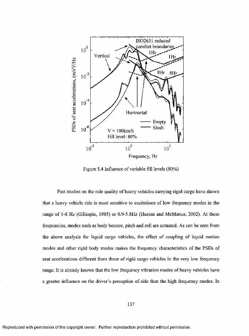
PS
Ds
of s
eat a
ccel
erat
ions
, (m
/s2)
2/H
z
100
10 2
10.4
10 6
101
Vertical
ISO2631 reduced comfort boundaries
1Hr
Horizontal
- Empty
V = 100km/h - Slosh
Fill level: 80%
1 0o
Frequency, Hz
101
Figure 5.4 Influence of variable fill levels (80%)
Past studies on the ride quality of heavy vehicles carrying rigid cargo have shown
that a heavy vehicle ride is most sensitive to excitations of low frequency modes in the
range of 1-8 Hz (Gillespie, 1985) or 0.9-5.8Hz (Hassan and McManus, 2002). At these
frequencies, modes such as body bounce, pitch and roll are actuated. As can be seen from
the above analysis for liquid cargo vehicles, the effect of coupling of liquid motion
modes and other rigid body modes makes the frequency characteristics of the PSDs of
seat accelerations different from those of rigid cargo vehicles in the very low frequency
range. It is already known that the low frequency vibration modes of heavy vehicles have
a greater influence on the driver's perception of ride than the high frequency modes. In
137
Reproduced with permission of the copyright owner. Further reproduction prohibited without permission.
N
EC
C/3co• rH
Idf-H<L>*3oocdod<uCOocoQC/3CL,
IS02631 reduced comfort boundaries. V v lH r1 X
010
Vertical
8 Hr 8Hr■20
410
Horizontal
EmptySlosh•6
10 V = lOOkm/h Fill level: 80%
l o l10 10 10
Frequency, Hz
Figure 5.4 Influence o f variable fill levels (80%)
Past studies on the ride quality of heavy vehicles carrying rigid cargo have shown
that a heavy vehicle ride is most sensitive to excitations of low frequency modes in the
range of 1-8 Hz (Gillespie, 1985) or 0.9-5.8Hz (Hassan and McManus, 2002). At these
frequencies, modes such as body bounce, pitch and roll are actuated. As can be seen from
the above analysis for liquid cargo vehicles, the effect of coupling o f liquid motion
modes and other rigid body modes makes the frequency characteristics o f the PSDs of
seat accelerations different from those o f rigid cargo vehicles in the very low frequency
range. It is already known that the low frequency vibration modes o f heavy vehicles have
a greater influence on the driver’s perception of ride than the high frequency modes. In
137
Reproduced with permission of the copyright owner. Further reproduction prohibited without permission.
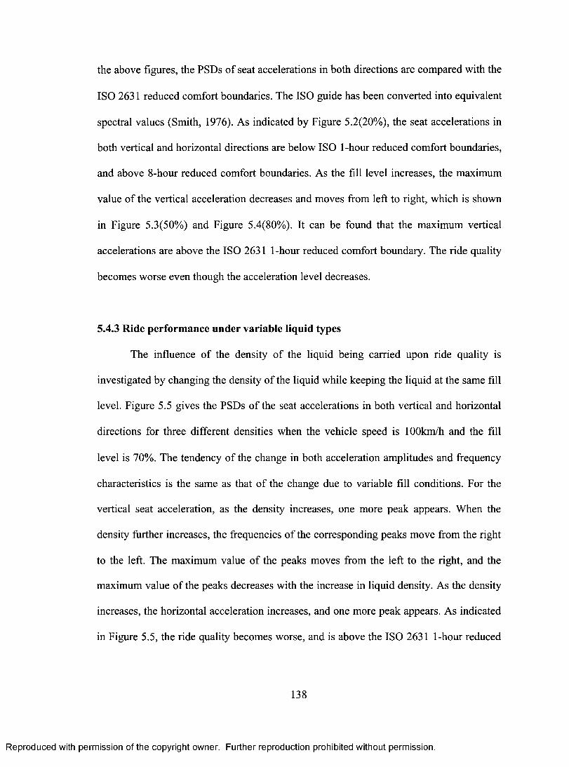
the above figures, the PSDs of seat accelerations in both directions are compared with the
ISO 2631 reduced comfort boundaries. The ISO guide has been converted into equivalent
spectral values (Smith, 1976). As indicated by Figure 5.2(20%), the seat accelerations in
both vertical and horizontal directions are below ISO 1-hour reduced comfort boundaries,
and above 8-hour reduced comfort boundaries. As the fill level increases, the maximum
value of the vertical acceleration decreases and moves from left to right, which is shown
in Figure 5.3(50%) and Figure 5.4(80%). It can be found that the maximum vertical
accelerations are above the ISO 2631 1-hour reduced comfort boundary. The ride quality
becomes worse even though the acceleration level decreases.
5.4.3 Ride performance under variable liquid types
The influence of the density of the liquid being carried upon ride quality is
investigated by changing the density of the liquid while keeping the liquid at the same fill
level. Figure 5.5 gives the PSDs of the seat accelerations in both vertical and horizontal
directions for three different densities when the vehicle speed is 100km/h and the fill
level is 70%. The tendency of the change in both acceleration amplitudes and frequency
characteristics is the same as that of the change due to variable fill conditions. For the
vertical seat acceleration, as the density increases, one more peak appears. When the
density further increases, the frequencies of the corresponding peaks move from the right
to the left. The maximum value of the peaks moves from the left to the right, and the
maximum value of the peaks decreases with the increase in liquid density. As the density
increases, the horizontal acceleration increases, and one more peak appears. As indicated
in Figure 5.5, the ride quality becomes worse, and is above the ISO 2631 1-hour reduced
138
Reproduced with permission of the copyright owner. Further reproduction prohibited without permission.
the above figures, the PSDs of seat accelerations in both directions are compared with the
ISO 2631 reduced comfort boundaries. The ISO guide has been converted into equivalent
spectral values (Smith, 1976). As indicated by Figure 5.2(20%), the seat accelerations in
both vertical and horizontal directions are below ISO 1-hour reduced comfort boundaries,
and above 8-hour reduced comfort boundaries. As the fill level increases, the maximum
value o f the vertical acceleration decreases and moves from left to right, which is shown
in Figure 5.3(50%) and Figure 5.4(80%). It can be found that the maximum vertical
accelerations are above the ISO 2631 1-hour reduced comfort boundary. The ride quality
becomes worse even though the acceleration level decreases.
5.4.3 Ride performance under variable liquid types
The influence of the density o f the liquid being carried upon ride quality is
investigated by changing the density o f the liquid while keeping the liquid at the same fill
level. Figure 5.5 gives the PSDs of the seat accelerations in both vertical and horizontal
directions for three different densities when the vehicle speed is lOOkm/h and the fill
level is 70%. The tendency of the change in both acceleration amplitudes and frequency
characteristics is the same as that of the change due to variable fill conditions. For the
vertical seat acceleration, as the density increases, one more peak appears. When the
density further increases, the frequencies o f the corresponding peaks move from the right
to the left. The maximum value of the peaks moves from the left to the right, and the
maximum value of the peaks decreases with the increase in liquid density. As the density
increases, the horizontal acceleration increases, and one more peak appears. As indicated
in Figure 5.5, the ride quality becomes worse, and is above the ISO 2631 1-hour reduced
138
Reproduced with permission of the copyright owner. Further reproduction prohibited without permission.
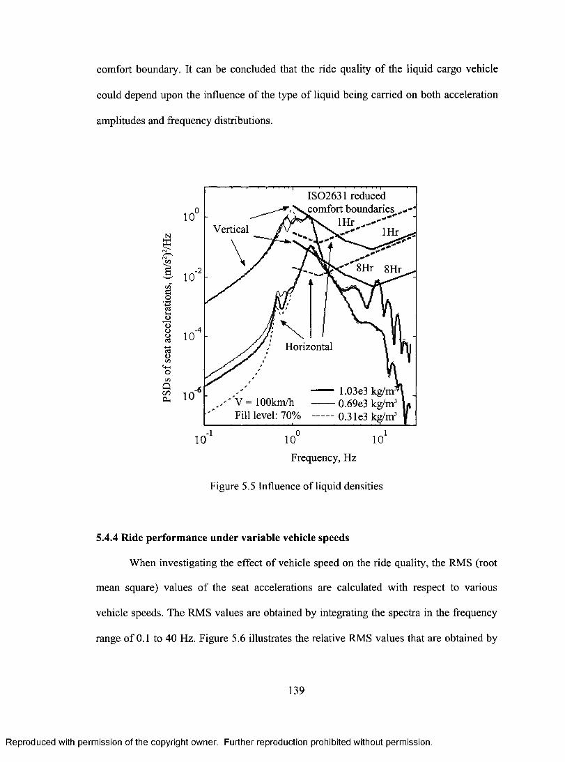
comfort boundary. It can be concluded that the ride quality of the liquid cargo vehicle
could depend upon the influence of the type of liquid being carried on both acceleration
amplitudes and frequency distributions.
PS
Ds
of s
eat a
ccel
erat
ions
, (m
/s2)
2/H
z
100
10 2
10 4
1a 6
.-------F'Vertical
IS02631 reduced comfort boundaries ..-d-• ....
Horizontal
' , 1.03e3 kg/m „ ..
,''V = 1001an/h — 0.69e3 kg/m -'- Fill level: 70% 0.31e3 1(4,/m
1Hr ........" ... ...0 1Hr
1 0- 1
10
Frequency, Hz
101
Figure 5.5 Influence of liquid densities
5.4.4 Ride performance under variable vehicle speeds
When investigating the effect of vehicle speed on the ride quality, the RMS (root
mean square) values of the seat accelerations are calculated with respect to various
vehicle speeds. The RMS values are obtained by integrating the spectra in the frequency
range of 0.1 to 40 Hz. Figure 5.6 illustrates the relative RMS values that are obtained by
139
Reproduced with permission of the copyright owner. Further reproduction prohibited without permission.
comfort boundary. It can be concluded that the ride quality o f the liquid cargo vehicle
could depend upon the influence o f the type of liquid being carried on both acceleration
amplitudes and frequency distributions.
N
5
G.2cdjB13oocdodvC/5
oC/5
Qc/oPh
Vertical
IS02631 reduced comfort boundaries -
: 8 Hr 8 Hr
Horizontal
-l10
V = lOOkm/h Fill level: 70%
1.03e3 kg/m" 0.69e3 kg/m3 0.3 le3 kg/m3
10 10
Frequency, Hz
Figure 5.5 Influence o f liquid densities
5.4.4 Ride performance under variable vehicle speeds
When investigating the effect o f vehicle speed on the ride quality, the RMS (root
mean square) values of the seat accelerations are calculated with respect to various
vehicle speeds. The RMS values are obtained by integrating the spectra in the frequency
range o f 0.1 to 40 Hz. Figure 5.6 illustrates the relative RMS values that are obtained by
139
Reproduced with permission of the copyright owner. Further reproduction prohibited without permission.
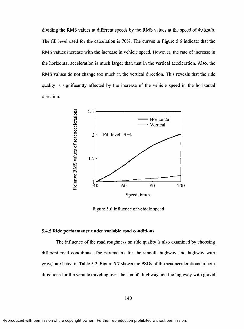
dividing the RMS values at different speeds by the RMS values at the speed of 40 km/h.
The fill level used for the calculation is 70%. The curves in Figure 5.6 indicate that the
RMS values increase with the increase in vehicle speed. However, the rate of increase in
the horizontal acceleration is much larger than that in the vertical acceleration. Also, the
RMS values do not change too much in the vertical direction. This reveals that the ride
quality is significantly affected by the increase of the vehicle speed in the horizontal
direction.
Rel
ativ
e R
MS
val
ues
of s
eat a
ccel
erat
ions
Speed, km/h
Figure 5.6 Influence of vehicle speed
5.4.5 Ride performance under variable road conditions
The influence of the road roughness on ride quality is also examined by choosing
different road conditions. The parameters for the smooth highway and highway with
gravel are listed in Table 5.2. Figure 5.7 shows the PSDs of the seat accelerations in both
directions for the vehicle traveling over the smooth highway and the highway with gravel
140
Reproduced with permission of the copyright owner. Further reproduction prohibited without permission.
dividing the RMS values at different speeds by the RMS values at the speed of 40 km/h.
The fill level used for the calculation is 70%. The curves in Figure 5.6 indicate that the
RMS values increase with the increase in vehicle speed. However, the rate o f increase in
the horizontal acceleration is much larger than that in the vertical acceleration. Also, the
RMS values do not change too much in the vertical direction. This reveals that the ride
quality is significantly affected by the increase o f the vehicle speed in the horizontal
direction.
t /3flO
<DOocamcawc/3CmOC/3<D
la>oo
<D.>Mca
&
2.5
HorizontalVertical
Fill level: 70%
40 80 100
Speed, km/h
Figure 5.6 Influence of vehicle speed
5.4.5 Ride performance under variable road conditions
The influence o f the road roughness on ride quality is also examined by choosing
different road conditions. The parameters for the smooth highway and highway with
gravel are listed in Table 5.2. Figure 5.7 shows the PSDs of the seat accelerations in both
directions for the vehicle traveling over the smooth highway and the highway with gravel
140
Reproduced with permission of the copyright owner. Further reproduction prohibited without permission.
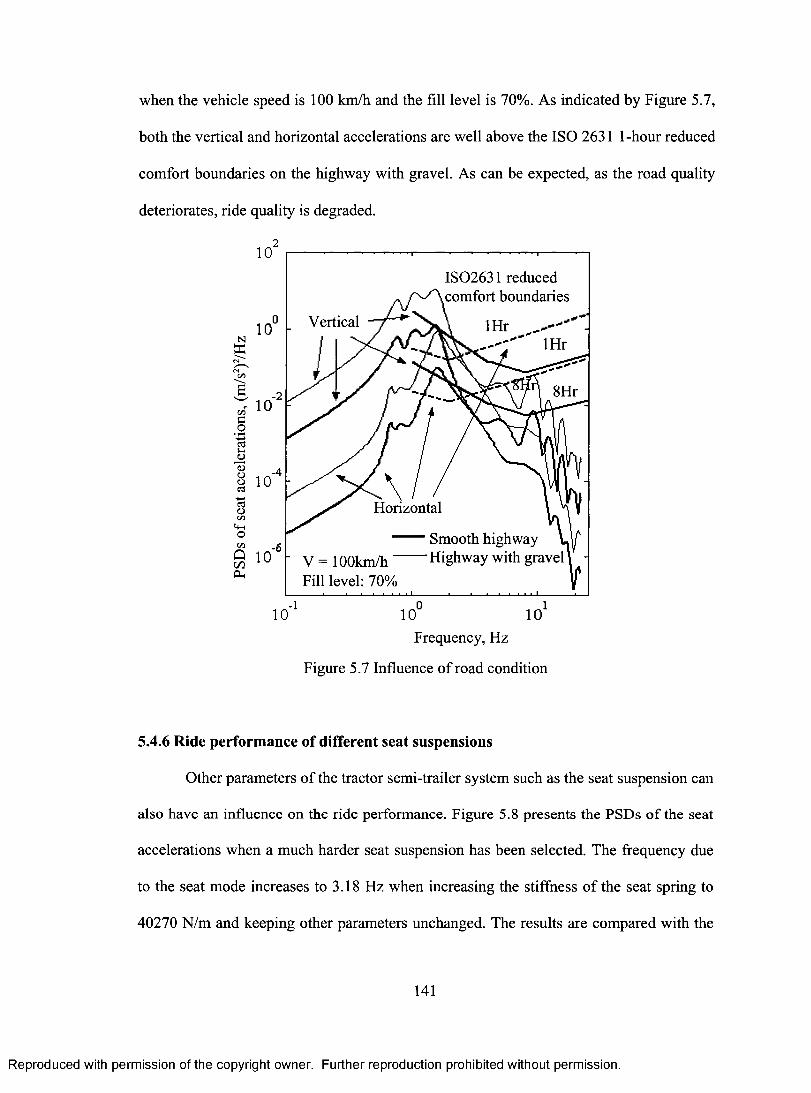
when the vehicle speed is 100 km/h and the fill level is 70%. As indicated by Figure 5.7,
both the vertical and horizontal accelerations are well above the ISO 2631 1-hour reduced
comfort boundaries on the highway with gravel. As can be expected, as the road quality
deteriorates, ride quality is degraded.
10 2
le Vertical
ISO2631 reduced comfortboundaries
4 , . .. . . . - : -, - - •
1Hr
„. ..1Hr _,
r".
v ial ,8Hr 1414'
V
'tHorizontal
V = 100km/h Fill level: 70%
Smooth highway Highway with gravel
101 100
Frequency, Hz
101
Figure 5.7 Influence of road condition
5.4.6 Ride performance of different seat suspensions
Other parameters of the tractor semi-trailer system such as the seat suspension can
also have an influence on the ride performance. Figure 5.8 presents the PSDs of the seat
accelerations when a much harder seat suspension has been selected. The frequency due
to the seat mode increases to 3.18 Hz when increasing the stiffness of the seat spring to
40270 N/m and keeping other parameters unchanged. The results are compared with the
141
Reproduced with permission of the copyright owner. Further reproduction prohibited without permission.
when the vehicle speed is 100 km/h and the fill level is 70%. As indicated by Figure 5.7,
both the vertical and horizontal accelerations are well above the ISO 2631 1-hour reduced
comfort boundaries on the highway with gravel. As can be expected, as the road quality
deteriorates, ride quality is degraded.
N
C/3c_oc3
jo73ooCCj<uC/3Cmo1/3
pmPh
10
IS02631 reduced comfort boundaries
o Vertical lH rlH r
10
8Hr■210
■40
Horizontal
Smooth highway I Highway with gravel
■60 V = lOOkm/h"
Fill level: 70%l o l
10 10 10Frequency, Hz
Figure 5.7 Influence of road condition
5.4.6 Ride performance of different seat suspensions
Other parameters o f the tractor semi-trailer system such as the seat suspension can
also have an influence on the ride performance. Figure 5.8 presents the PSDs o f the seat
accelerations when a much harder seat suspension has been selected. The frequency due
to the seat mode increases to 3.18 Hz when increasing the stiffness of the seat spring to
40270 N/m and keeping other parameters unchanged. The results are compared with the
141
Reproduced with permission of the copyright owner. Further reproduction prohibited without permission.
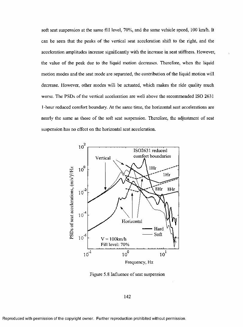
soft seat suspension at the same fill level, 70%, and the same vehicle speed, 100 km/h. It
can be seen that the peaks of the vertical seat acceleration shift to the right, and the
acceleration amplitudes increase significantly with the increase in seat stiffness. However,
the value of the peak due to the liquid motion decreases. Therefore, when the liquid
motion modes and the seat mode are separated, the contribution of the liquid motion will
decrease. However, other modes will be actuated, which makes the ride quality much
worse. The PSDs of the vertical acceleration are well above the recommended ISO 2631
1-hour reduced comfort boundary. At the same time, the horizontal seat accelerations are
nearly the same as those of the soft seat suspension. Therefore, the adjustment of seat
suspension has no effect on the horizontal seat acceleration.
PS
Ds
of s
eat a
ccel
erat
ions
, (m
/s2)
Z/H
z
102
100
10-2
1a 4
10 6
Vertical
ISO2631 reduced comfort boundaries
•-• 1Hr .------- ... -
1Hr
Horizontal
- Hard - Soft
V = 100km/h Fill level: 70%
. . . . . . . . . . . . ,
1 04
10 101
Frequency, Hz
Figure 5.8 Influence of seat suspension
142
Reproduced with permission of the copyright owner. Further reproduction prohibited without permission.
soft seat suspension at the same fill level, 70%, and the same vehicle speed, 100 km/h. It
can be seen that the peaks of the vertical seat acceleration shift to the right, and the
acceleration amplitudes increase significantly with the increase in seat stiffness. However,
the value of the peak due to the liquid motion decreases. Therefore, when the liquid
motion modes and the seat mode are separated, the contribution o f the liquid motion will
decrease. However, other modes will be actuated, which makes the ride quality much
worse. The PSDs of the vertical acceleration are well above the recommended ISO 2631
1-hour reduced comfort boundary. At the same time, the horizontal seat accelerations are
nearly the same as those of the soft seat suspension. Therefore, the adjustment o f seat
suspension has no effect on the horizontal seat acceleration.
10'2
IS02631 reducedcomfort boundariesVertical
Horizontal
V = lOOkm/h Fill level: 70%
10-l
10o
10Frequency, Hz
Figure 5.8 Influence o f seat suspension
142
Reproduced with permission of the copyright owner. Further reproduction prohibited without permission.
5.5 Summary
In this chapter, the ride performance of partially filled compartmented tank
vehicles has been investigated using a linearized multi-degree-of-freedom dynamic
model. The liquid motion in the partially filled tank is described as a linear spring-mass
model. The power spectral density of the vertical and horizontal seat accelerations has
been utilized to study the influence of liquid motion on ride quality. Since the natural
frequencies due to the liquid motion modes are in the very low range and are quite close
to those of the bounce and pitch modes, the effect of the coupling of these vibration
modes makes the ride quality quite different from that of the rigid cargo vehicles in the
very low frequency range. Simulation results show that the acceleration amplitudes and
frequency distributions are significantly affected by fill level, vehicle speed, road
condition, and the type of liquid being carried.
143
Reproduced with permission of the copyright owner. Further reproduction prohibited without permission.
5.5 Summary
In this chapter, the ride performance o f partially filled compartmented tank
vehicles has been investigated using a linearized multi-degree-of-freedom dynamic
model. The liquid motion in the partially filled tank is described as a linear spring-mass
model. The power spectral density o f the vertical and horizontal seat accelerations has
been utilized to study the influence o f liquid motion on ride quality. Since the natural
frequencies due to the liquid motion modes are in the very low range and are quite close
to those of the bounce and pitch modes, the effect o f the coupling of these vibration
modes makes the ride quality quite different from that o f the rigid cargo vehicles in the
very low frequency range. Simulation results show that the acceleration amplitudes and
frequency distributions are significantly affected by fill level, vehicle speed, road
condition, and the type of liquid being carried.
143
Reproduced with permission of the copyright owner. Further reproduction prohibited without permission.
CHAPTER 6 INFLUENCE OF NONLINEAR IMPACT ON
LIQUID CARGO TANK VEHICLES
6.1 Introduction
Although the mathematical method developed in Chapter 4 can be employed to
study the longitudinal dynamics for coupled liquid-vehicle-road systems under normal
driving conditions, it cannot deal with nonlinear impact problems during rough road
driving. The impact problem of liquid sloshing cannot be analytically solved. Other
methods, such as experimental studies (Kobayashi et al, 1989, Ye, 1990, Ye and Birk,
1990), numerical simulations (Arai et al, 1994, Kim, 2001), and equivalent mechanical
models (Ibrahim et al, 2001), have been employed in past investigations. Arai et al (1994)
developed a numerical method to simulate the impact load on tank walls and ceilings by
using the Marker-and-Cell (MAC) method for 3D rectangular containers. Due to the
discrete modeling of flow in the tank during the liquid impact on the tank ceiling, the
sudden change of boundary conditions from the free surface to the rigid one was detected
only at selected points in space. Therefore, the numerical solution of pressure time
history consisted of a series of isolated pulses that were generated at discrete grid points.
The authors used a numerical approach that mitigated this artificial discrete pressure
pulse in order to overcome this problem. Kim (2001) simulated sloshing with an impact
on the ceiling in 2D and 3D rectangular containers based on the Navier-Stokes equations,
finite difference method and SOLA scheme (Hirt et al, 1975). The concept of a buffer
zone was adopted near the tank ceiling, where a mixed boundary condition of rigid wall
and free surface was imposed before an impact. In order to mitigate a series of discrete
144
Reproduced with permission of the copyright owner. Further reproduction prohibited without permission.
CHAPTER 6 INFLUENCE OF NONLINEAR IMPACT ON
LIQUID CARGO TANK VEHICLES
6.1 Introduction
Although the mathematical method developed in Chapter 4 can be employed to
study the longitudinal dynamics for coupled liquid-vehicle-road systems under normal
driving conditions, it cannot deal with nonlinear impact problems during rough road
driving. The impact problem of liquid sloshing cannot be analytically solved. Other
methods, such as experimental studies (Kobayashi et al, 1989, Ye, 1990, Ye and Birk,
1990), numerical simulations (Arai et al, 1994, Kim, 2001), and equivalent mechanical
models (Ibrahim et al, 2001), have been employed in past investigations. Arai et al (1994)
developed a numerical method to simulate the impact load on tank walls and ceilings by
using the Marker-and-Cell (MAC) method for 3D rectangular containers. Due to the
discrete modeling o f flow in the tank during the liquid impact on the tank ceiling, the
sudden change of boundary conditions from the free surface to the rigid one was detected
only at selected points in space. Therefore, the numerical solution o f pressure time
history consisted of a series o f isolated pulses that were generated at discrete grid points.
The authors used a numerical approach that mitigated this artificial discrete pressure
pulse in order to overcome this problem. Kim (2001) simulated sloshing with an impact
on the ceiling in 2D and 3D rectangular containers based on the Navier-Stokes equations,
finite difference method and SOLA scheme (Hirt et al, 1975). The concept o f a buffer
zone was adopted near the tank ceiling, where a mixed boundary condition o f rigid wall
and free surface was imposed before an impact. In order to mitigate a series of discrete
144
Reproduced with permission of the copyright owner. Further reproduction prohibited without permission.
impacts, the computed signal was averaged over several time steps. The simulation
results showed a favourable agreement of impact pressures as well as the global fluid
motion.
However, the above methods can only be effective for a fairly gentle touch of
liquid on the ceiling. As pointed out by Arai et al (1994), in the case of violent sloshing,
such as nearly flat impact, the combined boundary condition was not effective. Generally
speaking, the numerical simulation of impact sloshing problems needs an extremely fine
mesh and time step, which will cause an extremely high demand for CPU time and
memory. For large amplitude excitations, the liquid becomes violent, and the stability of
numerical simulation can hardly be achieved. Impact is a quite challenging area in
sloshing studies.
An equivalent mechanical impact model was adopted by Pilipchuk and Ibrahim
(1997) and El-sayad et al (1999). Instead of pursuing the sloshing load by fluid
mechanics equations, the authors adopted an analogous pendulum model to simulate the
strongly nonlinear motion, where the nonlinearity was mainly due to the rapid velocity
changes associated with hydrodynamic pressure impacts of liquid motion close to the free
surface. The fluid free surface was modeled as a pendulum that could reach the walls of
the tank. Instead of using the equations of linear relationship with constraints, the authors
employed impact characteristic functions such as power nonlinearity with a higher
exponent to produce the same effect as the impact system. When the liquid model
described by the pendulum with hydrodynamic impact was included in the structural
system, the system model was obtained as multi-dimensional vibration equations with
both impact nonlinear terms and other nonlinear terms such as geometrical nonlinearities.
145
Reproduced with permission of the copyright owner. Further reproduction prohibited without permission.
impacts, the computed signal was averaged over several time steps. The simulation
results showed a favourable agreement o f impact pressures as well as the global fluid
motion.
However, the above methods can only be effective for a fairly gentle touch of
liquid on the ceiling. As pointed out by Arai et al (1994), in the case o f violent sloshing,
such as nearly flat impact, the combined boundary condition was not effective. Generally
speaking, the numerical simulation of impact sloshing problems needs an extremely fine
mesh and time step, which will cause an extremely high demand for CPU time and
memory. For large amplitude excitations, the liquid becomes violent, and the stability of
numerical simulation can hardly be achieved. Impact is a quite challenging area in
sloshing studies.
An equivalent mechanical impact model was adopted by Pilipchuk and Ibrahim
(1997) and El-sayad et al (1999). Instead of pursuing the sloshing load by fluid
mechanics equations, the authors adopted an analogous pendulum model to simulate the
strongly nonlinear motion, where the nonlinearity was mainly due to the rapid velocity
changes associated with hydrodynamic pressure impacts o f liquid motion close to the free
surface. The fluid free surface was modeled as a pendulum that could reach the walls of
the tank. Instead of using the equations of linear relationship with constraints, the authors
employed impact characteristic functions such as power nonlinearity with a higher
exponent to produce the same effect as the impact system. When the liquid model
described by the pendulum with hydrodynamic impact was included in the structural
system, the system model was obtained as multi-dimensional vibration equations with
both impact nonlinear terms and other nonlinear terms such as geometrical nonlinearities.
145
Reproduced with permission of the copyright owner. Further reproduction prohibited without permission.
This method has been used to study the dynamics of elastically supported elevated water
towers by the multiple scale method (El-sayad et al, 1999) and a special saw-tooth time
transformation technique (Pilipchuk and Ibrahim, 1997).
For liquid motion in horizontal cylindrical tanks, it is already known that the free
liquid surface motion and the liquid impact can be more severe longitudinally than
laterally if no transverse baffles are introduced (Ibrahim et al, 2001). An experimental
study was conducted by Kobayashi et al (1989) to determine the liquid natural
frequencies and the resultant slosh forces under small and large slosh wave heights in
horizontal cylindrical tanks, both laterally and longitudinally. The measured longitudinal
slosh forces, including the impulsive forces, were much larger than the calculated ones of
the linear theory. Compared with the stability analysis and directional response
characteristics of heavy vehicles carrying liquid cargo in the roll plane vehicle model, the
influence of liquid sloshing in the pitch plane has only been investigated in limited
studies. Only linear mechanical models were employed to represent the complex liquid
motion, and constant deceleration braking characteristics were considered. Rough road
conditions have never been included in the past investigations.
Equivalent mechanical models can be used for liquid cargo vehicle systems in
simulating vehicle behaviour. In this chapter, a nonlinear impact mechanical model for
liquid sloshing in partially filled liquid tank vehicles has been developed to investigate
the longitudinal dynamic characteristics of tank vehicles during typical straight-line
driving. The dynamic fluid motion within the tank has been modeled by utilizing a
mechanical system that can describe the behaviour of the liquid motion as a spring-mass
sloshing model with an impact subsystem for longitudinal oscillations. Computer
146
Reproduced with permission of the copyright owner. Further reproduction prohibited without permission.
This method has been used to study the dynamics of elastically supported elevated water
towers by the multiple scale method (El-sayad et al, 1999) and a special saw-tooth time
transformation technique (Pilipchuk and Ibrahim, 1997).
For liquid motion in horizontal cylindrical tanks, it is already known that the free
liquid surface motion and the liquid impact can be more severe longitudinally than
laterally if no transverse baffles are introduced (Ibrahim et al, 2001). An experimental
study was conducted by Kobayashi et al (1989) to determine the liquid natural
frequencies and the resultant slosh forces under small and large slosh wave heights in
horizontal cylindrical tanks, both laterally and longitudinally. The measured longitudinal
slosh forces, including the impulsive forces, were much larger than the calculated ones of
the linear theory. Compared with the stability analysis and directional response
characteristics o f heavy vehicles carrying liquid cargo in the roll plane vehicle model, the
influence o f liquid sloshing in the pitch plane has only been investigated in limited
studies. Only linear mechanical models were employed to represent the complex liquid
motion, and constant deceleration braking characteristics were considered. Rough road
conditions have never been included in the past investigations.
Equivalent mechanical models can be used for liquid cargo vehicle systems in
simulating vehicle behaviour. In this chapter, a nonlinear impact mechanical model for
liquid sloshing in partially filled liquid tank vehicles has been developed to investigate
the longitudinal dynamic characteristics o f tank vehicles during typical straight-line
driving. The dynamic fluid motion within the tank has been modeled by utilizing a
mechanical system that can describe the behaviour o f the liquid motion as a spring-mass
sloshing model with an impact subsystem for longitudinal oscillations. Computer
146
Reproduced with permission of the copyright owner. Further reproduction prohibited without permission.
simulation of the tank vehicle under typical rough road conditions has been performed by
incorporating the forces and moments caused by liquid motion into the pitch plane
vehicle model. The fifth wheel loads and the normal axle loads have been computed
using the mechanical system approach in order to investigate the influence of liquid
motion.
6.2 Nonlinear impact model of liquid sloshing
Equivalent mechanical models have been proven to be simple and effective ways
to describe the liquid slosh because the equations of motion for point masses and rigid
bodies could be included more readily in the overall vehicle model than the equations for
a continuously deformable medium such as fuel oil. Linear analytical representations of
liquid sloshing by the pendulum theory and spring-mass theory were usually employed in
liquid cargo vehicle research. In this section, the spring-mass model including nonlinear
impact effect has been developed to investigate the dynamics of liquid sloshing under
large amplitude situations.
For sloshing in the longitudinal direction of horizontal cylindrical tanks,
Ranganathan et al (1994) developed a summation technique to calculate the parameters of
the spring-mass model according to theory of the slosh response in rectangular tanks.
Kobayashi et al (1989) established an equivalent calculation method to make use of the
theory of slosh response in rectangular tanks in seismic design research. Calculated
results of natural frequencies are in good agreement with the experimental ones. This
calculation method was introduced in Section 4.4.1 and has been applied in studying the
ride quality problem for tractor semi-trailer systems in Chapter 5.
147
Reproduced with permission of the copyright owner. Further reproduction prohibited without permission.
simulation o f the tank vehicle under typical rough road conditions has been performed by
incorporating the forces and moments caused by liquid motion into the pitch plane
vehicle model. The fifth wheel loads and the normal axle loads have been computed
using the mechanical system approach in order to investigate the influence o f liquid
motion.
6.2 Nonlinear impact model of liquid sloshing
Equivalent mechanical models have been proven to be simple and effective ways
to describe the liquid slosh because the equations o f motion for point masses and rigid
bodies could be included more readily in the overall vehicle model than the equations for
a continuously deformable medium such as fuel oil. Linear analytical representations of
liquid sloshing by the pendulum theory and spring-mass theory were usually employed in
liquid cargo vehicle research. In this section, the spring-mass model including nonlinear
impact effect has been developed to investigate the dynamics o f liquid sloshing under
large amplitude situations.
For sloshing in the longitudinal direction o f horizontal cylindrical tanks,
Ranganathan et al (1994) developed a summation technique to calculate the parameters of
the spring-mass model according to theory o f the slosh response in rectangular tanks.
Kobayashi et al (1989) established an equivalent calculation method to make use o f the
theory o f slosh response in rectangular tanks in seismic design research. Calculated
results of natural frequencies are in good agreement with the experimental ones. This
calculation method was introduced in Section 4.4.1 and has been applied in studying the
ride quality problem for tractor semi-trailer systems in Chapter 5.
147
Reproduced with permission of the copyright owner. Further reproduction prohibited without permission.
When the liquid motion is described by a linear mechanical model, the equation
of motion is:
d 2x,, dx,imn1 dt 2 +CO dt + KnIx n = —Mnla x (6.1)
In this equation, innl, cn1 and k,,1 are equivalent mass, damping and stiffness of the
equivalent mass-spring system, and zn is the displacement of the mass. ax is the applied
acceleration on the equivalent mass.
Under severe conditions, nonlinear liquid motion will appear due to rapid velocity
changes associated with hydrodynamic pressure impacts. For example, this strongly
nonlinear motion could happen when the exciting frequency is equal to or near the
sloshing frequency. The resulting forces and moments caused by the hydrodynamic
pressure impact will affect the responses of the tank vehicles, and are extremely
important in design of the supporting structures and internal components of the vehicle
tanks. Pilipchuk and Ibrahim (1997) studied the nonlinear liquid sloshing impact in
moving rectangular containers. The liquid sloshing was modeled by a pendulum
describing impacts with the container walls. The mathematic model included the
constraint that 18„l < Ono when considering the pendulum and the container walls as rigid
bodies, where on was the pendulum angle, and e, was the angular when the pendulum
reached the container walls. To solve the problem, impact characteristic functions could
be used to produce the same effect as the linear equation with constraints.
Similarly, it is assumed that Ixa l< x,,0 is the constraint for the linear spring-mass
system for liquid slosh, where zno = w/2 . w is the longitudinal length of the tank
148
Reproduced with permission of the copyright owner. Further reproduction prohibited without permission.
When the liquid motion is described by a linear mechanical model, the equation
o f motion is:
d 2x n dxnm nl — j - + cnX — + k nXx n = - m nlax (6.1)
dt dt
In this equation, mn\,c„\ and kn\ are equivalent mass, damping and stiffness of the
equivalent mass-spring system, and x„ is the displacement o f the mass. ax is the applied
acceleration on the equivalent mass.
Under severe conditions, nonlinear liquid motion will appear due to rapid velocity
changes associated with hydrodynamic pressure impacts. For example, this strongly
nonlinear motion could happen when the exciting frequency is equal to or near the
sloshing frequency. The resulting forces and moments caused by the hydrodynamic
pressure impact will affect the responses o f the tank vehicles, and are extremely
important in design of the supporting structures and internal components o f the vehicle
tanks. Pilipchuk and Ibrahim (1997) studied the nonlinear liquid sloshing impact in
moving rectangular containers. The liquid sloshing was modeled by a pendulum
describing impacts with the container walls. The mathematic model included the
constraint that \en | < enQ when considering the pendulum and the container walls as rigid
bodies, where Qn was the pendulum angle, and was the angular when the pendulum
reached the container walls. To solve the problem, impact characteristic functions could
be used to produce the same effect as the linear equation with constraints.
Similarly, it is assumed that \xn \ < x n0 is the constraint for the linear spring-mass
system for liquid slosh, where xn0=w/2 . w is the longitudinal length o f the tank
148
Reproduced with permission of the copyright owner. Further reproduction prohibited without permission.
compartment. The potential energy function is (Pilipchuk and Ibrahim 1997) expressed
as:
ri(xj=bnxn0 xn
2nn
-\ 2n„
(6.2)
In this equation, nn >> 1 is a positive integer and bn is a positive constant parameter. The
impact force is:
Fm =
dInxn
) =
bn
„ (6.3)
Thus the equation of motion (6.1) can be modified to include the impact effect.
d2 xn dxn—
nin1 dt 2 + cn1 dt + kn,Xn bn
( xn
\Xn0
\ 2n„-1
= —Mnl a x
The motion equation can be expressed in the non-dimensional form.
2 dx
c 24-a) + con x + qnxc2 n 1 = — ax
dt n
dx
dt xno
(6.4)
(6.5)
According to Dodge (Abramson and Silverman, 1966), even considering the
energy dissipation due to free surface effects, the total dissipation or damping is so small
in unbaffled tanks that practically no limit is placed on the slosh amplitude at resonance.
By neglecting the damping effect, the interaction between the liquid and the tank walls
can be expressed as:
Fs = Mn1Can2Xn bnXc 11" -1 (6.6)
bn =gmmnixn0 (6.7)
xc = Xn0
xn
149
(6.8)
Reproduced with permission of the copyright owner. Further reproduction prohibited without permission.
compartment. The potential energy function is (Pilipchuk and Ibrahim 1997) expressed
as:
/ \2«„
2 n(6 .2)
n V nO /
In this equation, nn » 1 is a positive integer and b„ is a positive constant parameter. The
impact force is:
F _ d n k ) _ bim j r,dx„
(6.3)
Thus the equation o f motion (6.1) can be modified to include the impact effect.
md 2x dx
n\ + C n\ ------ + knXXn + bnd t 2 nx dt " "
/ ' \ 2 « „ - l
I ’± .
\ X nO J
~ mnxax (6.4)
The motion equation can be expressed in the non-dimensional form.
d 2x, dxc— f + 2 f r n —d t 1
2 2n -1 a rM + ^ n Xc +flnXc" = -----“dt X«0
(6.5)
According to Dodge (Abramson and Silverman, 1966), even considering the
energy dissipation due to free surface effects, the total dissipation or damping is so small
in unbaffled tanks that practically no limit is placed on the slosh amplitude at resonance.
By neglecting the damping effect, the interaction between the liquid and the tank walls
can be expressed as:
F s = m n \ ( ° 2n X n + ( 6 - 6 )
K = (6.7)
x„ = ■x,
(6 .8)n 0
149
Reproduced with permission of the copyright owner. Further reproduction prohibited without permission.
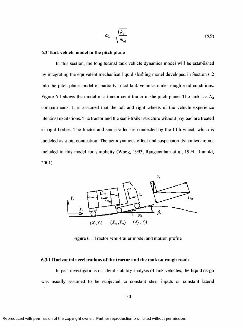
con , ‘
icil
Inn] (6.9)
6.3 Tank vehicle model in the pitch plane
In this section, the longitudinal tank vehicle dynamics model will be established
by integrating the equivalent mechanical liquid sloshing model developed in Section 6.2
into the pitch plane model of partially filled tank vehicles under rough road conditions.
Figure 6.1 shows the model of a tractor semi-trailer in the pitch plane. The tank has Nn
compartments. It is assumed that the left and right wheels of the vehicle experience
identical excitations. The tractor and the semi-trailer structure without payload are treated
as rigid bodies. The tractor and semi-trailer are connected by the fifth wheel, which is
modeled as a pin connection. The aerodynamics effect and suspension dynamics are not
included in this model for simplicity (Wong, 1993, Ranganathan et al, 1994, Rumold,
2001).
Vn
an
(X,., Yr) (Xm , Y„,) (Xf , Yf)
Figure 6.1 Tractor semi-trailer model and motion profile
6.3.1 Horizontal accelerations of the tractor and the tank on rough roads
In past investigations of lateral stability analysis of tank vehicles, the liquid cargo
was usually assumed to be subjected to constant steer inputs or constant lateral
150
Reproduced with permission of the copyright owner. Further reproduction prohibited without permission.
6.3 Tank vehicle model in the pitch plane
In this section, the longitudinal tank vehicle dynamics model will be established
by integrating the equivalent mechanical liquid sloshing model developed in Section 6.2
into the pitch plane model of partially filled tank vehicles under rough road conditions.
Figure 6.1 shows the model of a tractor semi-trailer in the pitch plane. The tank has Nn
compartments. It is assumed that the left and right wheels o f the vehicle experience
identical excitations. The tractor and the semi-trailer structure without payload are treated
as rigid bodies. The tractor and semi-trailer are connected by the fifth wheel, which is
modeled as a pin connection. The aerodynamics effect and suspension dynamics are not
included in this model for simplicity (Wong, 1993, Ranganathan et al, 1994, Rumold,
2001).
Vn
(Xr,Yr) (Xm,Ym) (Xf , Yj)
Figure 6.1 Tractor semi-trailer model and motion profile
6.3.1 Horizontal accelerations of the tractor and the tank on rough roads
In past investigations o f lateral stability analysis o f tank vehicles, the liquid cargo
was usually assumed to be subjected to constant steer inputs or constant lateral
150
Reproduced with permission of the copyright owner. Further reproduction prohibited without permission.
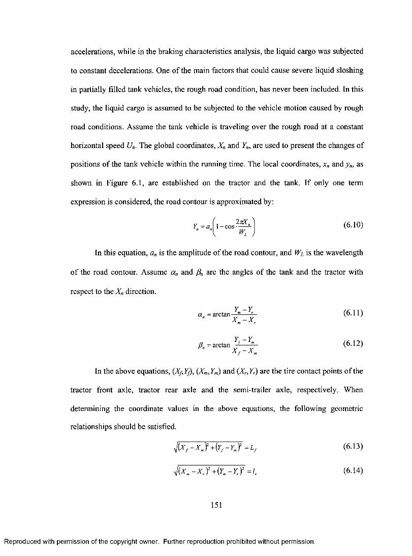
accelerations, while in the braking characteristics analysis, the liquid cargo was subjected
to constant decelerations. One of the main factors that could cause severe liquid sloshing
in partially filled tank vehicles, the rough road condition, has never been included. In this
study, the liquid cargo is assumed to be subjected to the vehicle motion caused by rough
road conditions. Assume the tank vehicle is traveling over the rough road at a constant
horizontal speed U. The global coordinates, X, and Yn, are used to present the changes of
positions of the tank vehicle within the running time. The local coordinates, x, and yn, as
shown in Figure 6.1, are established on the tractor and the tank. If only one term
expression is considered, the road contour is approximated by:
=a„ 1 —cos t „WL,
(6.10)
In this equation, an is the amplitude of the road contour, and WL is the wavelength
of the road contour. Assume an and fin are the angles of the tank and the tractor with
respect to the X, direction.
= arctan Y — Y
X. — X,
— Y /3 „ arctan
X — X„,
(6.11)
(6.12)
In the above equations, (, cf,Yf), Y,n) and (Xr, Yr) are the tire contact points of the
tractor front axle, tractor rear axle and the semi-trailer axle, respectively. When
determining the coordinate values in the above equations, the following geometric
relationships should be satisfied.
AI f + frf = Lf (6.13)
AAA'. — X,Y+(Y. —1c)2 =1,
151
(6.14)
Reproduced with permission of the copyright owner. Further reproduction prohibited without permission.
accelerations, while in the braking characteristics analysis, the liquid cargo was subjected
to constant decelerations. One of the main factors that could cause severe liquid sloshing
in partially filled tank vehicles, the rough road condition, has never been included. In this
study, the liquid cargo is assumed to be subjected to the vehicle motion caused by rough
road conditions. Assume the tank vehicle is traveling over the rough road at a constant
horizontal speed Un. The global coordinates, X„ and Yn, are used to present the changes of
positions o f the tank vehicle within the running time. The local coordinates, xn and y„, as
shown in Figure 6.1, are established on the tractor and the tank. If only one term
expression is considered, the road contour is approximated by:
Y'=a„' 2« r . Al - c o s (6.10)
WL
In this equation, an is the amplitude o f the road contour, and Wl is the wavelength
o f the road contour. Assume a„ and /?„ are the angles o f the tank and the tractor with
respect to the X n direction.
an = arctan — — — (6.11)
P n = arctan — ---- — (6.12)x f - x m
In the above equations, (Xf,YJ), (Xm,Ym) and (Xr, Yr) are the tire contact points o f the
tractor front axle, tractor rear axle and the semi-trailer axle, respectively. When
determining the coordinate values in the above equations, the following geometric
relationships should be satisfied.
f a , - x j +(¥,-¥„? =L{ (6.13)
y l (Xm - X r f + (Ym- Y r )2 =lr (6.14)
151
Reproduced with permission of the copyright owner. Further reproduction prohibited without permission.
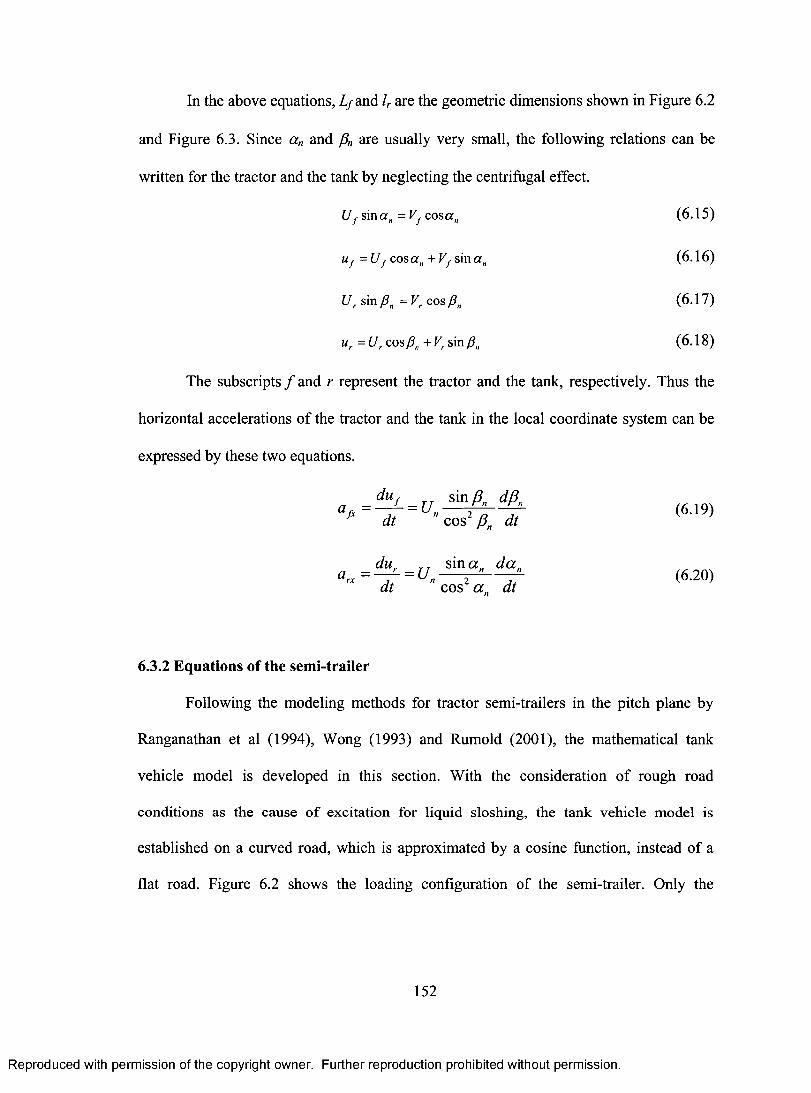
In the above equations, Lf and lr are the geometric dimensions shown in Figure 6.2
and Figure 6.3. Since an and fl are usually very small, the following relations can be
written for the tractor and the tank by neglecting the centrifugal effect.
Uf sin an =Vi cosan (6.15)
Uf =Uf cos an +Ili sin an (6.16)
Ur sin fi,, =v, cos fin (6.17)
u,. = U,. cos /fn + V, sin fin (6.18)
The subscripts f and r represent the tractor and the tank, respectively. Thus the
horizontal accelerations of the tractor and the tank in the local coordinate system can be
expressed by these two equations.
= du
f = U sin fi
" fx dt
ncos' 16 dt
a = dur = U sin a n dan
, dt n COS' a n dt
(6.19)
(6.20)
6.3.2 Equations of the semi-trailer
Following the modeling methods for tractor semi-trailers in the pitch plane by
Ranganathan et al (1994), Wong (1993) and Rumold (2001), the mathematical tank
vehicle model is developed in this section. With the consideration of rough road
conditions as the cause of excitation for liquid sloshing, the tank vehicle model is
established on a curved road, which is approximated by a cosine function, instead of a
flat road. Figure 6.2 shows the loading configuration of the semi-trailer. Only the
152
Reproduced with permission of the copyright owner. Further reproduction prohibited without permission.
In the above equations, Z/and lr are the geometric dimensions shown in Figure 6.2
and Figure 6.3. Since an and are usually very small, the following relations can be
written for the tractor and the tank by neglecting the centrifugal effect.
Uf sina„ = Vf cosan (6.15)
uf - Uf cos an + Vf sin an (6.16)
Ur sin p n = Vr cos /?„ (6.17)
ur = Ur cos Pn + Vr sin /?„ (6.18)
The subscripts / and r represent the tractor and the tank, respectively. Thus the
horizontal accelerations of the tractor and the tank in the local coordinate system can be
expressed by these two equations.
d u f s in /? dBa fx= — L = Un----- fa .— Bjl /6 19)dt cos Pn dt
dur TT s in«„ da„arX = - r - = U n (6-20)
dt cos a„ dt
6.3.2 Equations of the semi-trailer
Following the modeling methods for tractor semi-trailers in the pitch plane by
Ranganathan et al (1994), Wong (1993) and Rumold (2001), the mathematical tank
vehicle model is developed in this section. With the consideration of rough road
conditions as the cause o f excitation for liquid sloshing, the tank vehicle model is
established on a curved road, which is approximated by a cosine function, instead of a
flat road. Figure 6.2 shows the loading configuration of the semi-trailer. Only the
152
Reproduced with permission of the copyright owner. Further reproduction prohibited without permission.
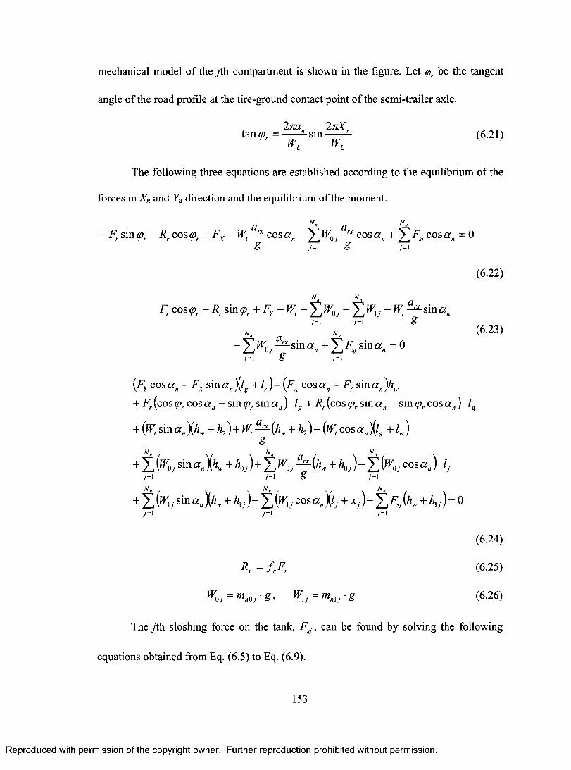
mechanical model of the jth compartment is shown in the figure. Let cor be the tangent
angle of the road profile at the tire-ground contact point of the semi-trailer axle.
27ran 27rX,tan g = sin
Wr. (6.21)
The following three equations are established according to the equilibrium of the
forces in X„ and Y,, direction and the equilibrium of the moment.
a — Fr sin q),. — Rr cos gor + Fx — a cos a,,—EWoi —1--x cos a„+ EFs; cos a n = 0
g j=1 g J=1
Fr cosyor — Rr sin g + Fy — TY, — EWoi — W arx sin a„ j=1 J=1
. —E W f a sin a„ +ZF s, sin a„= 0 o ./=-1 g f=1
(FY cosa„— Fx sin a n k+1,.)—(Fx cosa„+ Fy sin a n )h,,„
+ Fr (cosgor cosa„+ sin g sin a n ) lg +R,.(cosgor sin a,— sin go,. cos a n ) lg
+(W, sin a n Xiiw +h2 )+W, + h2 )— (W, cos a n k g +1,,)
+ E(wo; sin a n )(11„,+1101)+ZW0i —a"(17,„+hoi)—E(w0; cos a n ) 1 1=1 j=1 j=1 N„ N„ N„
+ E(wii sin a ii(h 1 j) — E(w11cos a ,,X1 + x j) — (11 „ + ) = 0 i=i i=i j=i
(6.22)
(6.23)
(6.24)
Rr = frFr (6.25)
WO j = nin0j • g W lj = innlj • g (6.26)
The jth sloshing force on the tank, Fsi , can be found by solving the following
equations obtained from Eq. (6.5) to Eq. (6.9).
153
Reproduced with permission of the copyright owner. Further reproduction prohibited without permission.
mechanical model o f the y'th compartment is shown in the figure. Let cpr be the tangent
angle o f the road profile at the tire-ground contact point of the semi-trailer axle.
tan (pr = sin 'n^ r (6.21)WL WL
The following three equations are established according to the equilibrium of the
forces in X n and Yn direction and the equilibrium of the moment.
a N" a N"- Fr s in (pr - Rr co s (pr + F X - fVt - nLc o sa n - 'Y 'fV 0, - SLc o sa n + Y f . c o s« n = 0
g M g M
(6 .22)
N „ N „
F, cos <?, - R , sin <pr + F , - W, - £ ,W0, - £ ,Wt, - W, ^ ;sin ,a ,7 =1 7 = 1 g
(6-23)" Z W oj — sin «„ + Z F s jsin a n = 0
7 = 1 g 7 = 1
far cos a n - F x s \n a n cos a n + Fy sin a n )hw
+ Fr (cos (pr cos a n + sin (pr sin a n) / + Rr (cos (pr sin a n - sin (pr cos a n) /
+ (Wt sin a n \ h w + h2 ) + Wt ^ (hw + h2) ■- (Wt cos a n \ l g + lw)§
N „ N n N „
+ Z S'm a n l K + f h j ) + ' L W 0 j — ( K + C 0 S a n) h7 = 1 7 = 1 g 7 = 1
N n N „ N „
+ £ (fV{J sin a n\ h w + hXJ)~ Z ( K j co sa n \ l j + x}) - £ K { K + K j ) = 07 = 1 7 = 1 7 = 1
(6.24)
R r = f rFr (6.25)
K j = ™„oj ■ g > W\j = mnXJ ■ g (6.26)
The yth sloshing force on the tank, Fsj, can be found by solving the following
equations obtained from Eq. (6.5) to Eq. (6.9).
153
Reproduced with permission of the copyright owner. Further reproduction prohibited without permission.
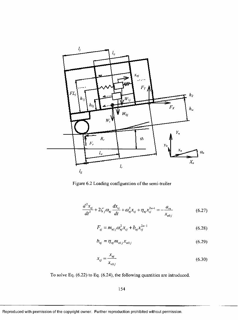
lg
Figure 6.2 Loading configuration of the semi-trailer
2 d X d.Xci 2n-1 a rx
COnix ci + niXci — dt 2
+ 24"Joni dt X nO j
2n-1 F sj = Mn1 j CO2nj Xcj b nj X cj
b nj = njni nlj Xn0j
X njX ci =
X nO j
To solve Eq. (6.22) to Eq. (6.24), the following quantities are introduced.
154
(6.27)
(6.28)
(6.29)
(6.30)
Reproduced with permission of the copyright owner. Further reproduction prohibited without permission.
r
Figure 6.2 Loading configuration o f the semi-trailer
d x . d x . , , , a - + 2C (D __ - + a> x + n x = __—dt1 ^ * dt + a ’ + '! Xmj
b nj = I n j ^ n X j ^ n O j
XnjX c j = —
X n O j
To solve Eq. (6.22) to Eq. (6.24), the following quantities are introduced.
154
(6.27)
(6.28)
(6.29)
(6.30)
Reproduced with permission of the copyright owner. Further reproduction prohibited without permission.
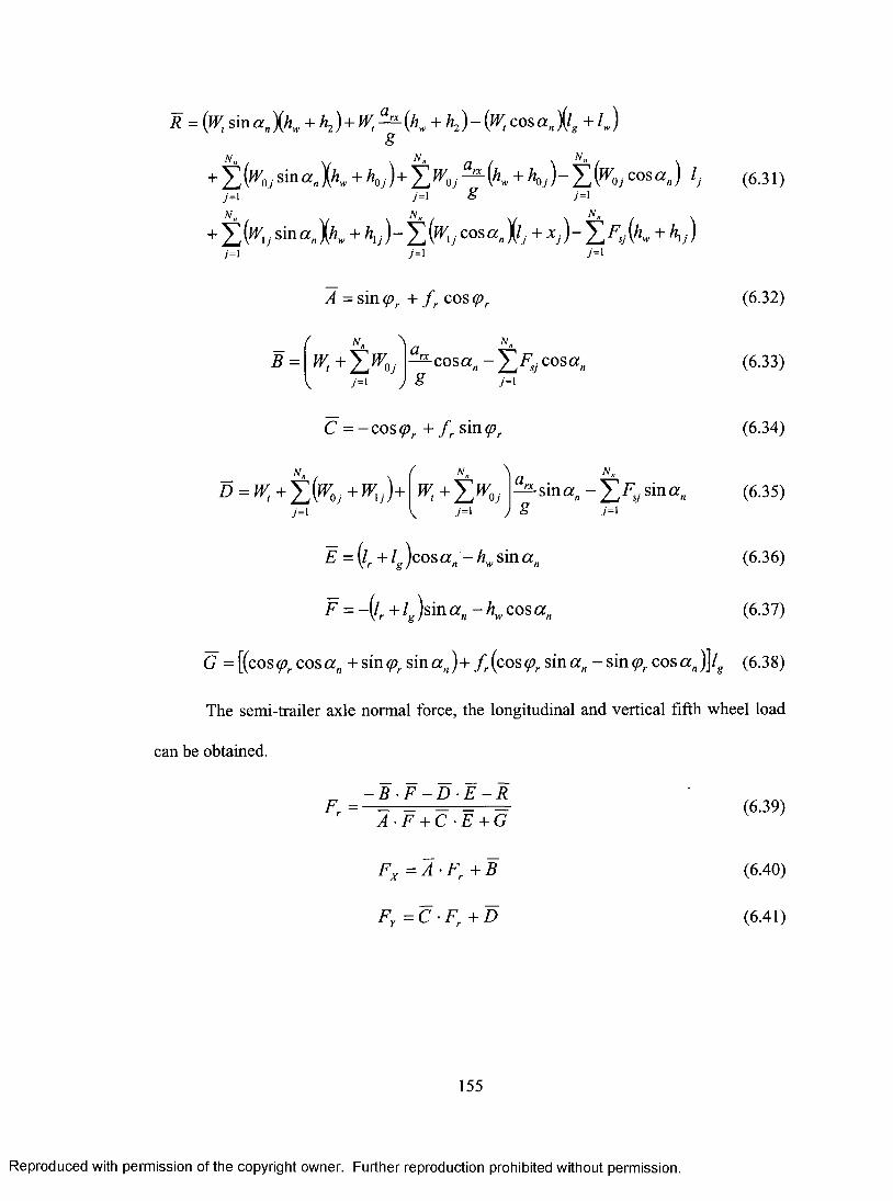
=(w, sin a„ )02„, + h2 )+ W, + 10—(47,cosan k g +1,„)
+1(W o j sin an )(h,,+ hc,j)+1Wo jarx (h„, + I/01 )— E(wojeosan) lJ
J=1 g J=1
+I(W1 j sin an k,+11,j)-1(wl cosa,,Xli +xj)-1F si(k+h,j) j=1 1=1
= sin cor + f r coso,.
I N„ N„
.E. = wt +lwoiarx
cosan —IFsi cosa„ J--1 j g j=1
=—cosq,r + f r sin gis,
N„ , N„
=wt +DK; -kwu)+ W +Iwo.;j=1 j=1
E =(1,.+1g )cosan — hw sin an
= —(1, + lg )sin an —h„,cosan
(6.31)
(6.32)
(6.33)
(6.34)
N„
arx sin an —IFs., sin a n (6.35) J=1
(6.36)
(6.37)
G = [(cos car cos an + sin car sin an )+ f. (cos cor sin an co,. cos (in )]lg (6.38)
The semi-trailer axle normal force, the longitudinal and vertical fifth wheel load
can be obtained.
Fr = —ff•F—D•k—k A•F+C•E+G
(6.39)
Fx =71•Fr +B (6.40)
Fy = C • Fr +D (6.41)
155
Reproduced with permission of the copyright owner. Further reproduction prohibited without permission.
R = (Wt s ina n\ h w + h2)+ ^ — (K + h2)-(jV, co sa n g + lw)g
+ Z K y sin a j h w + h0j)+ Y W 0J^ (hw + /*>,-)- Z K y co s««) h (6.31)j = 1 J = 1 £ / = !
N,
+ Z K Sin« J ^ + 0 ~ Z K ' c o sa J / . + X7) - Z ^ ( ^ + ^y)y=i y=i 7=i
B =N„ N„
wt + i w0j — cos«„ - I X cosa„7 = 1
C = - c o s (pr + f r s in <pr
N n f N n \ " n
D =Wt + Z (^ o y + W,j)+ Wt + Y W 0j — s i n - Z Fsjs i na nV 7 = 1 ) g7 = 1 7 = 1
E = ( l r + lg )cos a „ - hw sin a„
^ = - ( /r + ^ ) sin« i , - ^ cos a i.
(6.32)
(6.33)
(6.34)
(6.35)
(6.36)
(6.37)
G = [(cos <pr cos a n + sin cpr sin a n) + f r (cos (pr sin a n - sin (pr cos a n )]/g (6.38)
The semi-trailer axle normal force, the longitudinal and vertical fifth wheel load
can be obtained.
- B F - D E - R r ~ A - F + C -E + G
Fx = A • Fr + B
FV= C F + D
(6.39)
(6.40)
(6.41)
155
Reproduced with permission of the copyright owner. Further reproduction prohibited without permission.
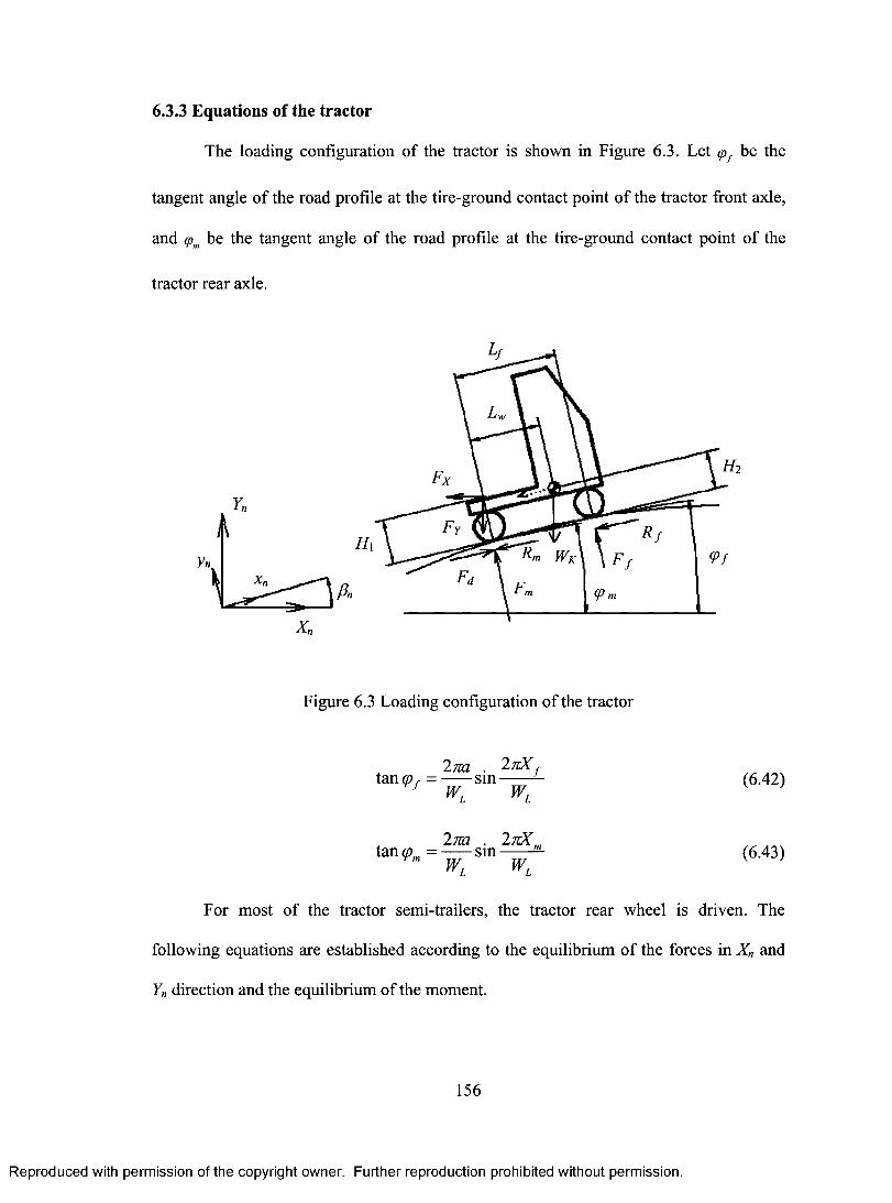
6.3.3 Equations of the tractor
The loading configuration of the tractor is shown in Figure 6.3. Let yof be the
tangent angle of the road profile at the tire-ground contact point of the tractor front axle,
and co,,, be the tangent angle of the road profile at the tire-ground contact point of the
tractor rear axle.
Yn
fin
Figure 6.3 Loading configuration of the tractor
tan go = 27-ca
sin 27TXf f WL WL
(6.42)
tan corn= 2ga
sin 27-rX.
(6.43) W W L L
For most of the tractor semi-trailers, the tractor rear wheel is driven. The
following equations are established according to the equilibrium of the forces in X, and
Yn direction and the equilibrium of the moment.
156
Reproduced with permission of the copyright owner. Further reproduction prohibited without permission.
6.3.3 Equations of the tractor
The loading configuration of the tractor is shown in Figure 6.3. Let q> be the
tangent angle o f the road profile at the tire-ground contact point o f the tractor front axle,
and (pm be the tangent angle of the road profile at the tire-ground contact point of the
tractor rear axle.
<Pf
Figure 6.3 Loading configuration o f the tractor
2 m . 2.7lKftane?, = s in (6.42)
Vr WL WL
2 m . 27tXmtan (pm = s in ^ (6.43)
WL WL V 7
For most o f the tractor semi-trailers, the tractor rear wheel is driven. The
following equations are established according to the equilibrium of the forces in X n and
Yn direction and the equilibrium of the moment.
156
Reproduced with permission of the copyright owner. Further reproduction prohibited without permission.
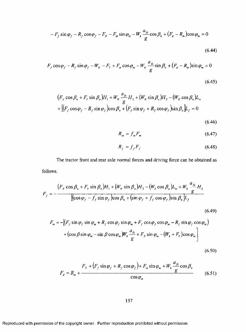
— Ff sin ypf — Rf cos col — Fx — Fm sin yom — Wk —arf cos fin + (Fd — Rm )cos yom = 0
(6.44)
Ff cos yo f — Rf sin yof — WK — Fy F„, cos q)„, — WK s.fx
sin fin + (Fd — Rm )sin q)„, = 0
(6.45)
(Fx cos fin + Fy sin fin + WK :2- H2 + (WK sin 13,,)H2 — O K cos )3 n )L,„ g
+[(F f cos yo f R f sin y)f )cos /3n + (Ff sin q)./. + R f cos q)./ )sin f = 0
(6.46)
= f„,Fm (6.47)
R f = ff Ff (6.48)
The tractor front and rear axle normal forces and driving force can be obtained as
follows.
Ft =
(Fx cos fin + Fy sin fin + (WK sin fin )H2 — (Wk cos fin )L,„ + Wk a
fx H2g
[(cos yof — f f sin yof )cos fin + (sin yof + f f cos yof )sin fin iLf
F„, = —{(Ff sin yof sin yom + Rf cos sin q). + Ff cos yof cos yom — Rf sin cos
+ (cos fi sin yom —sin fi cos yom )Wk 2c—fx
+ Fx sin q,„, —(Wk +Fy )coscpng
Fx + (F f sin gof R f COS f )± Fm sin yom + Wk afx cos i n
Fd = + cos q)„,
157
(6.49)
(6.50)
(6.51)
Reproduced with permission of the copyright owner. Further reproduction prohibited without permission.
(6.44)
Ff co s<pf - R f sin(pf - W K - F Y + Fm co s<pm - WK ^ s i n J3n + {Fd - Rm)s in (pm = 0§
(6.45)
(Fx cos A + F, sin A )f f , + ^ t f 2 + (WK sin A )ff 2 - cos A Kg
[(/*) cos (pf - R f sin <pf )cos Pn + {Ff sin (pf + Rf cos (pf )sin P ^ f = 0+
R ,n = f m F m
(6.46)
(6.47)
R f = f f F f (6.48)
The tractor front and rear axle normal forces and driving force can be obtained as
follows.
( f , cos A + Fr sin A )H , + (WK sin A ) # 2 - cos A ) A + ^ ^F f -
[(cos (pf - f f sin (pf )cos (3n + (sin <pf + f f cos <pf )sin P n ]Lfg
(6.49)
Fm = -[(.F} sin (pf sin (pm + Rf cos (pf sin (pm + Ff cos (pf cos cpm - Rf sin (pf cos (pm)
+ (cos p sin cpm - sin p cos <pm )Wk — + FX sin cpm - (Wk + Fy) cos <pmg
(6.50)
Fx + (1Ff sin <pf + Rf cos <pf )+ Fm sin (pm + Wk ^ c o s Pn ______________ _________ _ ________ s __
c o s ^(6.51)
157
Reproduced with permission of the copyright owner. Further reproduction prohibited without permission.
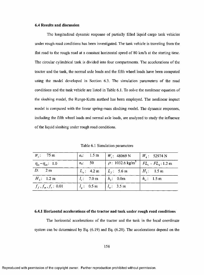
6.4 Results and discussion
The longitudinal dynamic response of partially filled liquid cargo tank vehicles
under rough road conditions has been investigated. The tank vehicle is traveling from the
flat road to the rough road at a constant horizontal speed of 80 km/h at the starting time.
The circular cylindrical tank is divided into four compartments. The accelerations of the
tractor and the tank, the normal axle loads and the fifth wheel loads have been computed
using the model developed in Section 6.3. The simulation parameters of the road
conditions and the tank vehicle are listed in Table 6.1. To solve the nonlinear equation of
the sloshing model, the Runge-Kutta method has been employed. The nonlinear impact
model is compared with the linear spring-mass sloshing model. The dynamic responses,
including the fifth wheel loads and normal axle loads, are analyzed to study the influence
of the liquid sloshing under rough road conditions.
Table 6.1 Simulation parameters
Pry 75 m an: 1.5 m W, : 48069 N Wk : 52974 N
IL --17,0 : 1.0 nn: 50 p : 1032.6 kg/m3 FL, - FL4 : 1.2 m
D: 2m L,„: 4.2m Lf : 5.6m HI : 1.5m
H 2 : 1.2 m lr : 7.0 m h2 : 0.0m lc: 1.5 m
f f , f„,,fr : 0.01 ig : 0.5m lw : 3.5m
6.4.1 Horizontal accelerations of the tractor and tank under rough road conditions
The horizontal accelerations of the tractor and the tank in the local coordinate
system can be determined by Eq. (6.19) and Eq. (6.20). The accelerations depend on the
158
Reproduced with permission of the copyright owner. Further reproduction prohibited without permission.
6.4 Results and discussion
The longitudinal dynamic response o f partially filled liquid cargo tank vehicles
under rough road conditions has been investigated. The tank vehicle is traveling from the
flat road to the rough road at a constant horizontal speed of 80 km/h at the starting time.
The circular cylindrical tank is divided into four compartments. The accelerations of the
tractor and the tank, the normal axle loads and the fifth wheel loads have been computed
using the model developed in Section 6.3. The simulation parameters o f the road
conditions and the tank vehicle are listed in Table 6.1. To solve the nonlinear equation of
the sloshing model, the Runge-Kutta method has been employed. The nonlinear impact
model is compared with the linear spring-mass sloshing model. The dynamic responses,
including the fifth wheel loads and normal axle loads, are analyzed to study the influence
o f the liquid sloshing under rough road conditions.
Table 6.1 Simulation parameters
WL: 75 m a„: 1.5 m Wt : 48069 N Wk : 52974 N
nnl-
orf1 n„: 50 P - 1032.6 kg/m3 F L X - F L a : 1.2 m
D: 2 m L w: 4.2 m L f 5.6 m H x: 1.5 m
h 2 : 1.2 m I/- 7.0 m h2, 0.0m K - 1.5 m
f f 0.01 h-- 0.5 m K-- 3.5 m
6.4.1 Horizontal accelerations of the tractor and tank under rough road conditions
The horizontal accelerations of the tractor and the tank in the local coordinate
system can be determined by Eq. (6.19) and Eq. (6.20). The accelerations depend on the
158
Reproduced with permission of the copyright owner. Further reproduction prohibited without permission.
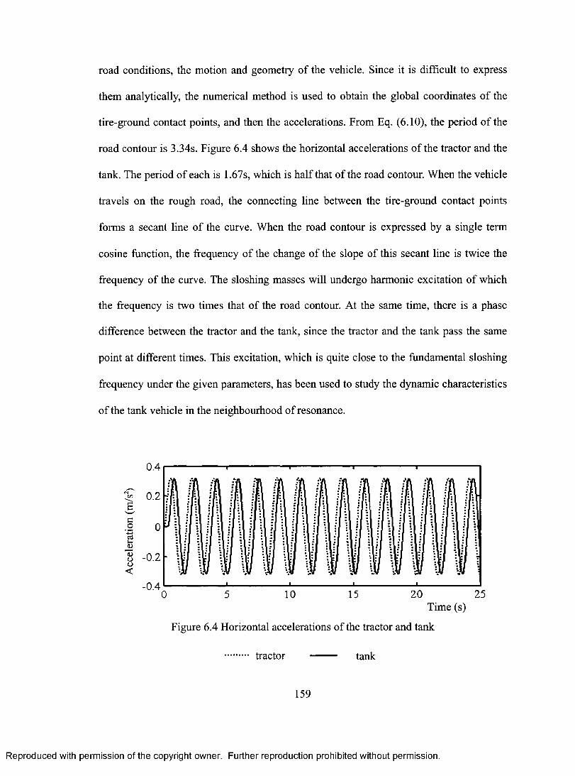
road conditions, the motion and geometry of the vehicle. Since it is difficult to express
them analytically, the numerical method is used to obtain the global coordinates of the
tire-ground contact points, and then the accelerations. From Eq. (6.10), the period of the
road contour is 3.34s. Figure 6.4 shows the horizontal accelerations of the tractor and the
tank. The period of each is 1.67s, which is half that of the road contour. When the vehicle
travels on the rough road, the connecting line between the tire-ground contact points
forms a secant line of the curve. When the road contour is expressed by a single term
cosine function, the frequency of the change of the slope of this secant line is twice the
frequency of the curve. The sloshing masses will undergo harmonic excitation of which
the frequency is two times that of the road contour. At the same time, there is a phase
difference between the tractor and the tank, since the tractor and the tank pass the same
point at different times. This excitation, which is quite close to the fundamental sloshing
frequency under the given parameters, has been used to study the dynamic characteristics
of the tank vehicle in the neighbourhood of resonance.
5 10 15 20 25 Time (s)
Figure 6.4 Horizontal accelerations of the tractor and tank
tractor tank
159
Reproduced with permission of the copyright owner. Further reproduction prohibited without permission.
road conditions, the motion and geometry o f the vehicle. Since it is difficult to express
them analytically, the numerical method is used to obtain the global coordinates of the
tire-ground contact points, and then the accelerations. From Eq. (6.10), the period o f the
road contour is 3.34s. Figure 6.4 shows the horizontal accelerations o f the tractor and the
tank. The period of each is 1.67s, which is half that o f the road contour. When the vehicle
travels on the rough road, the connecting line between the tire-ground contact points
forms a secant line o f the curve. When the road contour is expressed by a single term
cosine function, the frequency of the change of the slope of this secant line is twice the
frequency of the curve. The sloshing masses will undergo harmonic excitation of which
the frequency is two times that of the road contour. At the same time, there is a phase
difference between the tractor and the tank, since the tractor and the tank pass the same
point at different times. This excitation, which is quite close to the fundamental sloshing
frequency under the given parameters, has been used to study the dynamic characteristics
of the tank vehicle in the neighbourhood of resonance.
0.4
« 0.2
cq n
<D8 - 0.2 o <
-0.420
Time (s)
Figure 6.4 Horizontal accelerations o f the tractor and tank
tractor ------- tank
159
Reproduced with permission of the copyright owner. Further reproduction prohibited without permission.
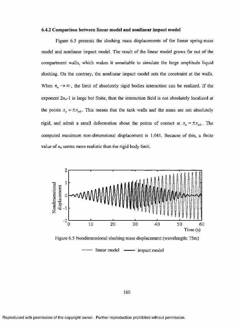
6.4.2 Comparison between linear model and nonlinear impact model
Figure 6.5 presents the sloshing mass displacements of the linear spring-mass
model and nonlinear impact model. The result of the linear model grows far out of the
compartment walls, which makes it unsuitable to simulate the large amplitude liquid
sloshing. On the contrary, the nonlinear impact model sets the constraint at the walls.
When n„ —) 00 , the limit of absolutely rigid bodies interaction can be realized. If the
exponent 2n,-1 is large but finite, then the interaction field is not absolutely localized at
the points xn = ±x,i0 . This means that the tank walls and the mass are not absolutely
rigid, and admit a small deformation about the points of contact at x„ = -±x,0 . The
computed maximum non-dimensional displacement is 1.041. Because of this, a finite
value of n„ seems more realistic than the rigid body limit.
• • 1 . _ 0 10 20 30 40 50 60
Time (s)
Figure 6.5 Nondimensional sloshing mass displacement (wavelength: 75m)
linear model — impact model
160
Reproduced with permission of the copyright owner. Further reproduction prohibited without permission.
6.4.2 Comparison between linear model and nonlinear impact model
Figure 6.5 presents the sloshing mass displacements o f the linear spring-mass
compartment walls, which makes it unsuitable to simulate the large amplitude liquid
sloshing. On the contrary, the nonlinear impact model sets the constraint at the walls.
When nn —> go , the limit of absolutely rigid bodies interaction can be realized. If the
exponent 2nn-\ is large but finite, then the interaction field is not absolutely localized at
the points x n — ± xn0. This means that the tank walls and the mass are not absolutely
rigid, and admit a small deformation about the points of contact at xn = ± xn0. The
computed maximum non-dimensional displacement is 1.041. Because o f this, a finite
value o f n„ seems more realistic than the rigid body limit.
model and nonlinear impact model. The result o f the linear model grows far out of the
2
2 ■ ■ ■ ■ ■" 0 10 20 30 40 50 60
Time (s)
Figure 6.5 Nondimensional sloshing mass displacement (wavelength: 75m)
linear model impact model
160
Reproduced with permission of the copyright owner. Further reproduction prohibited without permission.
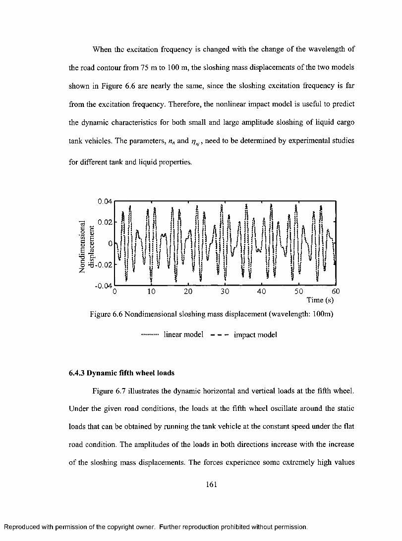
When the excitation frequency is changed with the change of the wavelength of
the road contour from 75 m to 100 m, the sloshing mass displacements of the two models
shown in Figure 6.6 are nearly the same, since the sloshing excitation frequency is far
from the excitation frequency. Therefore, the nonlinear impact model is useful to predict
the dynamic characteristics for both small and large amplitude sloshing of liquid cargo
tank vehicles. The parameters, nn and /in, , need to be determined by experimental studies
for different tank and liquid properties.
Non
dim
ensi
onal
0.04
1 A
)1 11 MI 11 11 Ji !ill 111 I IPA 11111.
- Vij il ihnj qf h
-0.04 0 10 20 30 40 50 60
Time (s)
Figure 6.6 Nondimensional sloshing mass displacement (wavelength: 100m)
linear model — — — impact model
6.4.3 Dynamic fifth wheel loads
Figure 6.7 illustrates the dynamic horizontal and vertical loads at the fifth wheel.
Under the given road conditions, the loads at the fifth wheel oscillate around the static
loads that can be obtained by running the tank vehicle at the constant speed under the flat
road condition. The amplitudes of the loads in both directions increase with the increase
of the sloshing mass displacements. The forces experience some extremely high values
161
Reproduced with permission of the copyright owner. Further reproduction prohibited without permission.
When the excitation frequency is changed with the change o f the wavelength of
the road contour from 75 m to 100 m, the sloshing mass displacements of the two models
shown in Figure 6 .6 are nearly the same, since the sloshing excitation frequency is far
from the excitation frequency. Therefore, the nonlinear impact model is useful to predict
the dynamic characteristics for both small and large amplitude sloshing o f liquid cargo
tank vehicles. The parameters, n„ and 77 ., need to be determined by experimental studies
for different tank and liquid properties.
0.04
0.02
-0.0420 30 40 50
Time (s)
Figure 6 .6 Nondimensional sloshing mass displacement (wavelength: 100m)
linear m o d e l impact model
6.4.3 Dynamic fifth wheel loads
Figure 6.7 illustrates the dynamic horizontal and vertical loads at the fifth wheel.
Under the given road conditions, the loads at the fifth wheel oscillate around the static
loads that can be obtained by running the tank vehicle at the constant speed under the flat
road condition. The amplitudes of the loads in both directions increase with the increase
o f the sloshing mass displacements. The forces experience some extremely high values
161
Reproduced with permission of the copyright owner. Further reproduction prohibited without permission.
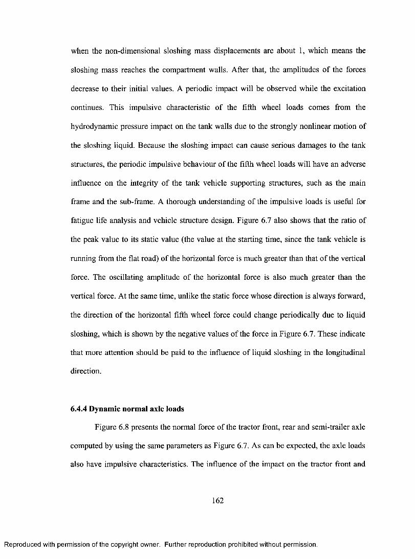
when the non-dimensional sloshing mass displacements are about 1, which means the
sloshing mass reaches the compartment walls. After that, the amplitudes of the forces
decrease to their initial values. A periodic impact will be observed while the excitation
continues. This impulsive characteristic of the fifth wheel loads comes from the
hydrodynamic pressure impact on the tank walls due to the strongly nonlinear motion of
the sloshing liquid. Because the sloshing impact can cause serious damages to the tank
structures, the periodic impulsive behaviour of the fifth wheel loads will have an adverse
influence on the integrity of the tank vehicle supporting structures, such as the main
frame and the sub-frame. A thorough understanding of the impulsive loads is useful for
fatigue life analysis and vehicle structure design. Figure 6.7 also shows that the ratio of
the peak value to its static value (the value at the starting time, since the tank vehicle is
running from the flat road) of the horizontal force is much greater than that of the vertical
force. The oscillating amplitude of the horizontal force is also much greater than the
vertical force. At the same time, unlike the static force whose direction is always forward,
the direction of the horizontal fifth wheel force could change periodically due to liquid
sloshing, which is shown by the negative values of the force in Figure 6.7. These indicate
that more attention should be paid to the influence of liquid sloshing in the longitudinal
direction.
6.4.4 Dynamic normal axle loads
Figure 6.8 presents the normal force of the tractor front, rear and semi-trailer axle
computed by using the same parameters as Figure 6.7. As can be expected, the axle loads
also have impulsive characteristics. The influence of the impact on the tractor front and
162
Reproduced with permission of the copyright owner. Further reproduction prohibited without permission.
when the non-dimensional sloshing mass displacements are about 1, which means the
sloshing mass reaches the compartment walls. After that, the amplitudes o f the forces
decrease to their initial values. A periodic impact will be observed while the excitation
continues. This impulsive characteristic o f the fifth wheel loads comes from the
hydrodynamic pressure impact on the tank walls due to the strongly nonlinear motion of
the sloshing liquid. Because the sloshing impact can cause serious damages to the tank
structures, the periodic impulsive behaviour o f the fifth wheel loads will have an adverse
influence on the integrity of the tank vehicle supporting structures, such as the main
frame and the sub-frame. A thorough understanding of the impulsive loads is useful for
fatigue life analysis and vehicle structure design. Figure 6.7 also shows that the ratio of
the peak value to its static value (the value at the starting time, since the tank vehicle is
running from the flat road) o f the horizontal force is much greater than that o f the vertical
force. The oscillating amplitude of the horizontal force is also much greater than the
vertical force. At the same time, unlike the static force whose direction is always forward,
the direction of the horizontal fifth wheel force could change periodically due to liquid
sloshing, which is shown by the negative values o f the force in Figure 6.7. These indicate
that more attention should be paid to the influence o f liquid sloshing in the longitudinal
direction.
6.4.4 Dynamic normal axle loads
Figure 6.8 presents the normal force o f the tractor front, rear and semi-trailer axle
computed by using the same parameters as Figure 6.7. As can be expected, the axle loads
also have impulsive characteristics. The influence o f the impact on the tractor front and
162
Reproduced with permission of the copyright owner. Further reproduction prohibited without permission.
rear axle normal forces is greater than that of the semi-trailer axle normal force. Since the
static liquid weight is mainly supported by the tractor rear and semi-trailer axle, the
average value of the tractor front axle normal force is much less than that of the tractor
rear and semi-trailer axle. Therefore, the investigation of the longitudinal stability of
partially filled tank vehicles under rough road conditions is focused on the tractor front
axle. Extreme cases can be seen in this figure. At the moment when the sloshing mass
reaches the compartment walls, the normal force of the tractor front axle becomes
negative, which in a real situation means the front wheel may lose contact with the road
surface at these particular instants. Though the force goes back to its equilibrium point
after the impacts, the possible liftoff of the front wheel may possibly cause instability of
tank vehicles under some extreme conditions, which may cause catastrophic accidents.
1
10 2.0 30 40 50 60 Time (s)
Figure 6.7 Fifth wheel loads
horizontal load vertical load
163
Reproduced with permission of the copyright owner. Further reproduction prohibited without permission.
rear axle normal forces is greater than that o f the semi-trailer axle normal force. Since the
static liquid weight is mainly supported by the tractor rear and semi-trailer axle, the
average value o f the tractor front axle normal force is much less than that o f the tractor
rear and semi-trailer axle. Therefore, the investigation of the longitudinal stability of
partially filled tank vehicles under rough road conditions is focused on the tractor front
axle. Extreme cases can be seen in this figure. At the moment when the sloshing mass
reaches the compartment walls, the normal force o f the tractor front axle becomes
negative, which in a real situation means the front wheel may lose contact with the road
surface at these particular instants. Though the force goes back to its equilibrium point
after the impacts, the possible liftoff of the front wheel may possibly cause instability of
tank vehicles under some extreme conditions, which may cause catastrophic accidents.
1
^ 0.555
VO0S 01 -°-5
-i0 10 20 30 40 50 60
Time (s)
Figure 6.7 Fifth wheel loads
horizontal load ------- vertical load
163
■ : j
v - v w V v v y W .........
Reproduced with permission of the copyright owner. Further reproduction prohibited without permission.
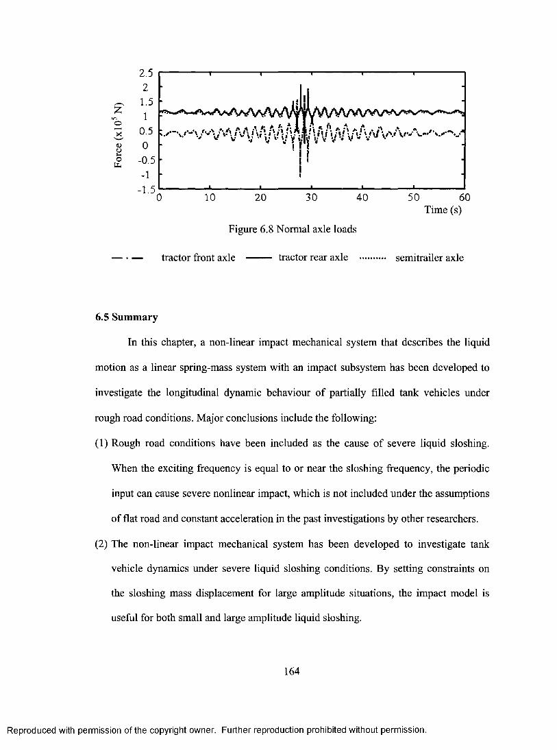
z
iG
a) 00
4.1
2.5 2
1.5
1 0.5 0
-0.5 -1
-1.50
e A ! • • f; A fl it A 4. NA; tIEV• IL/ I. • .iiii•il, •1.% ext t. Ai • i• v %.; • P xi 0 V
I I
10 20 30 40 50 60 Time (s)
Figure 6.8 Normal axle loads
tractor front axle tractor rear axle semitrailer axle
6.5 Summary
In this chapter, a non-linear impact mechanical system that describes the liquid
motion as a linear spring-mass system with an impact subsystem has been developed to
investigate the longitudinal dynamic behaviour of partially filled tank vehicles under
rough road conditions. Major conclusions include the following:
(1) Rough road conditions have been included as the cause of severe liquid sloshing.
When the exciting frequency is equal to or near the sloshing frequency, the periodic
input can cause severe nonlinear impact, which is not included under the assumptions
of flat road and constant acceleration in the past investigations by other researchers.
(2) The non-linear impact mechanical system has been developed to investigate tank
vehicle dynamics under severe liquid sloshing conditions. By setting constraints on
the sloshing mass displacement for large amplitude situations, the impact model is
useful for both small and large amplitude liquid sloshing.
164
Reproduced with permission of the copyright owner. Further reproduction prohibited without permission.
2.52
^ 1.5£oo* 0.5
-1-1.5
0 10 20 30 40 50 60Time (s)
Figure 6.8 Normal axle loads
tractor front axle tractor rear axle semitrailer axle
6.5 Summary
In this chapter, a non-linear impact mechanical system that describes the liquid
motion as a linear spring-mass system with an impact subsystem has been developed to
investigate the longitudinal dynamic behaviour o f partially filled tank vehicles under
rough road conditions. Major conclusions include the following:
(1) Rough road conditions have been included as the cause o f severe liquid sloshing.
When the exciting frequency is equal to or near the sloshing frequency, the periodic
input can cause severe nonlinear impact, which is not included under the assumptions
of flat road and constant acceleration in the past investigations by other researchers.
(2) The non-linear impact mechanical system has been developed to investigate tank
vehicle dynamics under severe liquid sloshing conditions. By setting constraints on
the sloshing mass displacement for large amplitude situations, the impact model is
useful for both small and large amplitude liquid sloshing.
164
Reproduced with permission of the copyright owner. Further reproduction prohibited without permission.
(3) Periodic impulsive behaviour of fifth wheel loads and normal axle loads is shown in
the neighbourhood of resonance. More attention should be paid to the fifth wheel load
in the horizontal direction in structure design and fatigue analysis, due to the drastic
changes in both the amplitude and the direction.
(4) Instability of the tank vehicle may occur under certain rough road conditions due to
the possible loss of tire-ground contact at the tractor front axle.
165
Reproduced with permission of the copyright owner. Further reproduction prohibited without permission.
(3) Periodic impulsive behaviour o f fifth wheel loads and normal axle loads is shown in
the neighbourhood o f resonance. More attention should be paid to the fifth wheel load
in the horizontal direction in structure design and fatigue analysis, due to the drastic
changes in both the amplitude and the direction.
(4) Instability of the tank vehicle may occur under certain rough road conditions due to
the possible loss o f tire-ground contact at the tractor front axle.
165
Reproduced with permission of the copyright owner. Further reproduction prohibited without permission.
CHAPTER 7 CONCLUSIONS AND RECOMMENDATIONS
7.1 Conclusions
In this dissertation, the dynamic behaviour of liquid motion inside liquid cargo
vehicle tanks has been investigated in detail based on the newly developed mathematical
method especially for liquid motion in horizontal cylindrical tanks. Liquid cargo vehicle
dynamics in the longitudinal direction has been investigated by equivalent mechanical
models for some situations where the newly developed method cannot be used, i.e., the
ride comfort problem in the frequency domain and the nonlinear impact problem in the
pitch plane.
The research involves: the development of a new mathematical method and
corresponding numerical procedures for liquid motion inside 2D circular and elliptical
tanks; the development of a new mathematical method for liquid motion inside 3D
horizontal cylindrical tanks with flat heads and hemispherical heads; a dynamic liquid
behaviour study based on the newly developed methods for both 2D and 3D road tanks
under typical highway operation conditions, such as turning, lane change and
braking/accelerating; the investigation of the ride quality of liquid cargo tank vehicles in
the longitudinal direction by integrating the equivalent linear mass-spring systems into
the tractor semi-trailer model; the study of the influence of liquid impact by the
development of an equivalent nonlinear impact model.
Research results from the author's research activities during his Ph.D. program
have been published in the form of journal papers, conference papers and a technical
report ([19, 20, 21, 22, 23, 130, 131, 132, 133, 134, 135, 136, 137]), most of which are
166
Reproduced with permission of the copyright owner. Further reproduction prohibited without permission.
CHAPTER 7 CONCLUSIONS AND RECOMMENDATIONS
7.1 Conclusions
In this dissertation, the dynamic behaviour o f liquid motion inside liquid cargo
vehicle tanks has been investigated in detail based on the newly developed mathematical
method especially for liquid motion in horizontal cylindrical tanks. Liquid cargo vehicle
dynamics in the longitudinal direction has been investigated by equivalent mechanical
models for some situations where the newly developed method cannot be used, i.e., the
ride comfort problem in the frequency domain and the nonlinear impact problem in the
pitch plane.
The research involves: the development o f a new mathematical method and
corresponding numerical procedures for liquid motion inside 2D circular and elliptical
tanks; the development of a new mathematical method for liquid motion inside 3D
horizontal cylindrical tanks with flat heads and hemispherical heads; a dynamic liquid
behaviour study based on the newly developed methods for both 2D and 3D road tanks
under typical highway operation conditions, such as turning, lane change and
braking/accelerating; the investigation o f the ride quality of liquid cargo tank vehicles in
the longitudinal direction by integrating the equivalent linear mass-spring systems into
the tractor semi-trailer model; the study of the influence of liquid impact by the
development of an equivalent nonlinear impact model.
Research results from the author’s research activities during his Ph.D. program
have been published in the form of journal papers, conference papers and a technical
report ([19, 20, 21, 22, 23, 130, 131, 132, 133, 134, 135, 136, 137]), most o f which are
166
Reproduced with permission of the copyright owner. Further reproduction prohibited without permission.
directly from this dissertation. The major conclusions of the research presented in this
work are as follows.
• A new mathematical method to solve the dynamic liquid behaviour in partially
filled horizontal 2D circular and elliptical tanks has been developed to study the
lateral dynamics of liquid motion inside road tanks. The governing equations for
the liquid motion in a tank are manipulated with the continuous coordinate
transformations. The first transformation saves the performance of interpolation
of boundary conditions on the curved walls. The application of the second
transformation changes the working domain to a fixed area, avoiding the complex
algorithm for free surface updating and volume correction. When the governing
equations are solved using the finite difference method, the third transformation is
adopted to gain computational convergence and stability.
• Compared with some other numerical schemes for sloshing problems in 2D
circular tanks, there are some advantages to the current method. The current
method does not need to deal with the boundary conditions on the time varying
curved walls and free surface. There is no need for capturing or smoothing of the
free surface, and the performance of volume correction. Complicated algorithms
for interpolation on rigid walls and updating the free surface are completely
avoided. These make the algorithm efficient and stable. The governing equations
are rearranged so that the programming is easy. Replacement of different
transformation equations for the first transformation can be easily carried out in
the same way for tanks with arbitrary wall shapes. Replacement of different
167
Reproduced with permission of the copyright owner. Further reproduction prohibited without permission.
directly from this dissertation. The major conclusions o f the research presented in this
work are as follows.
• A new mathematical method to solve the dynamic liquid behaviour in partially
filled horizontal 2D circular and elliptical tanks has been developed to study the
lateral dynamics o f liquid motion inside road tanks. The governing equations for
the liquid motion in a tank are manipulated with the continuous coordinate
transformations. The first transformation saves the performance of interpolation
o f boundary conditions on the curved walls. The application o f the second
transformation changes the working domain to a fixed area, avoiding the complex
algorithm for free surface updating and volume correction. When the governing
equations are solved using the finite difference method, the third transformation is
adopted to gain computational convergence and stability.
• Compared with some other numerical schemes for sloshing problems in 2D
circular tanks, there are some advantages to the current method. The current
method does not need to deal with the boundary conditions on the time varying
curved walls and free surface. There is no need for capturing or smoothing of the
free surface, and the performance o f volume correction. Complicated algorithms
for interpolation on rigid walls and updating the free surface are completely
avoided. These make the algorithm efficient and stable. The governing equations
are rearranged so that the programming is easy. Replacement o f different
transformation equations for the first transformation can be easily carried out in
the same way for tanks with arbitrary wall shapes. Replacement o f different
167
Reproduced with permission of the copyright owner. Further reproduction prohibited without permission.
transformation equations for the transformations can also be done without much
extra modification needed for program codes in adjusting the grid distribution.
• More importantly, the new method has an excellent capability of extending to
solve liquid motion in 3D horizontal cylindrical tanks subjected to excitations in
both longitudinal and lateral directions. It has been concluded in the literature
review that the combination of 3D vehicle models with 2D dynamic liquid motion
have been used to simulate vehicle dynamics by considering only the lateral liquid
motion with the assumption that liquid at all cross sections behaves identically in
the transversal direction. The lack of an effective algorithm to describe the liquid
motion in 3D space constrained past researches to the steady turning operation. At
the same time, researches on liquid cargo vehicles in the longitudinal direction
were often carried out on rectangular tanks instead of horizontal cylindrical ones,
for the same reason. In this research, a new mathematical method has been
developed to study the liquid dynamics in partially filled 3D horizontal cylindrical
tanks based on the method developed for 2D circular and elliptical tanks. This
approach provides a useful tool for solving the liquid dynamics in horizontal
cylindrical road tanks in a completely 3D manner. It can be easily integrated into
coupled liquid-structure systems to study the vehicle system dynamics. This also
provides the availability of a systematic analysis of tank vehicle structures
subjected to liquid sloshing and other loadings.
• During turning operations, the newly developed method has been used to simulate
168
Reproduced with permission of the copyright owner. Further reproduction prohibited without permission.
transformation equations for the transformations can also be done without much
extra modification needed for program codes in adjusting the grid distribution.
• More importantly, the new method has an excellent capability o f extending to
solve liquid motion in 3D horizontal cylindrical tanks subjected to excitations in
both longitudinal and lateral directions. It has been concluded in the literature
review that the combination o f 3D vehicle models with 2D dynamic liquid motion
have been used to simulate vehicle dynamics by considering only the lateral liquid
motion with the assumption that liquid at all cross sections behaves identically in
the transversal direction. The lack o f an effective algorithm to describe the liquid
motion in 3D space constrained past researches to the steady turning operation. At
the same time, researches on liquid cargo vehicles in the longitudinal direction
were often carried out on rectangular tanks instead of horizontal cylindrical ones,
for the same reason. In this research, a new mathematical method has been
developed to study the liquid dynamics in partially filled 3D horizontal cylindrical
tanks based on the method developed for 2D circular and elliptical tanks. This
approach provides a useful tool for solving the liquid dynamics in horizontal
cylindrical road tanks in a completely 3D manner. It can be easily integrated into
coupled liquid-structure systems to study the vehicle system dynamics. This also
provides the availability of a systematic analysis o f tank vehicle structures
subjected to liquid sloshing and other loadings.
• During turning operations, the newly developed method has been used to simulate
168
Reproduced with permission of the copyright owner. Further reproduction prohibited without permission.
the oscillatory liquid motion that could not be described by mass centre models.
The oscillatory motion depends on the acceleration input time and the final
acceleration amplitude. The oscillation amplitude of the liquid motion increases
with the increase in steady acceleration. The oscillation amplitude decreases with
an increase of the input time. A suddenly applied acceleration without an input
time causes the largest oscillatory amplitude and should be avoided in the
operation. The dynamic liquid motion during a lane change operation and a
double lane change has also been calculated.
• Longitudinal dynamic liquid motion inside 3D horizontal cylindrical tanks has
been analyzed by the new method during accelerating/braking operations. When
the tank is subjected to a suddenly applied acceleration, the liquid inside the tank
undergoes oscillatory motion, which significantly changes the pressure
distributions on the tank walls. This causes oscillatory forces and moments on the
tank. Larger acceleration causes larger forces and moments in both mean values
and extreme values. Compared to the free surface shapes in tanks with flat heads,
the free surfaces inside the tank with hemispherical heads are much flatter. The
influence of higher modes is quite weak due to the existence of the curved head
walls. For compartmented tanks with different fill levels, the asynchronous liquid
motion helps to decrease the magnitude of the varying force when the resultant
liquid force is obtained by combining the forces in all compartments. Long tanks
without any partitions are harmful for longitudinal dynamics and are therefore a
bad choice for carrying liquid product.
169
Reproduced with permission of the copyright owner. Further reproduction prohibited without permission.
the oscillatory liquid motion that could not be described by mass centre models.
The oscillatory motion depends on the acceleration input time and the final
acceleration amplitude. The oscillation amplitude of the liquid motion increases
with the increase in steady acceleration. The oscillation amplitude decreases with
an increase o f the input time. A suddenly applied acceleration without an input
time causes the largest oscillatory amplitude and should be avoided in the
operation. The dynamic liquid motion during a lane change operation and a
double lane change has also been calculated.
• Longitudinal dynamic liquid motion inside 3D horizontal cylindrical tanks has
been analyzed by the new method during accelerating/braking operations. When
the tank is subjected to a suddenly applied acceleration, the liquid inside the tank
undergoes oscillatory motion, which significantly changes the pressure
distributions on the tank walls. This causes oscillatory forces and moments on the
tank. Larger acceleration causes larger forces and moments in both mean values
and extreme values. Compared to the free surface shapes in tanks with flat heads,
the free surfaces inside the tank with hemispherical heads are much flatter. The
influence o f higher modes is quite weak due to the existence of the curved head
walls. For compartmented tanks with different fill levels, the asynchronous liquid
motion helps to decrease the magnitude o f the varying force when the resultant
liquid force is obtained by combining the forces in all compartments. Long tanks
without any partitions are harmful for longitudinal dynamics and are therefore a
bad choice for carrying liquid product.
169
Reproduced with permission of the copyright owner. Further reproduction prohibited without permission.
• The ride comfort for vehicle operations is of great concern because an exposure to
high levels of vibration will cause driver fatigue, which in turn can have a harmful
effect on health problems and driving safety. The liquid motion within the
partially filled tanks has a negative influence on the driver's ride quality, a
problem which had never been studied. In this research, the ride performance of
partially filled compartmented tank vehicles in the longitudinal direction has been
investigated by a linearized multi-degree-of-freedom dynamic model. The power
spectral density of the vertical and horizontal seat accelerations has been utilized
to study the influence of liquid motion on the ride quality. The frequencies due to
the liquid sloshing modes are in the frequency range of 0.1-0.7 Hz, which is
determined by the tank configurations and fill levels and quite close to the
frequencies due to the bounce and pitch modes, as well as the seat mode. This
generates a coupled effect on the frequency response, which makes the frequency
distribution in the range considered quite different from that of rigid cargo
vehicles in the low frequency domain, i.e., 0.1-2Hz. Simulation results show that
the amplitudes and frequency distributions of seat accelerations in both directions
are significantly affected by the liquid fill level, vehicle speed, road surface
condition, the type of liquid being carried, and the seat suspension parameters.
• Under severe conditions, highly nonlinear liquid motion will occur due to rapid
velocity changes associated with hydrodynamic pressure impacts. One of the
main factors that could cause severe liquid sloshing in partially filled tank
vehicles is the rough road surface. When the excitation frequency of the road
170
Reproduced with permission of the copyright owner. Further reproduction prohibited without permission.
• The ride comfort for vehicle operations is of great concern because an exposure to
high levels o f vibration will cause driver fatigue, which in turn can have a harmful
effect on health problems and driving safety. The liquid motion within the
partially filled tanks has a negative influence on the driver’s ride quality, a
problem which had never been studied. In this research, the ride performance of
partially filled compartmented tank vehicles in the longitudinal direction has been
investigated by a linearized multi-degree-of-ffeedom dynamic model. The power
spectral density o f the vertical and horizontal seat accelerations has been utilized
to study the influence of liquid motion on the ride quality. The frequencies due to
the liquid sloshing modes are in the frequency range o f 0.1-0.7 Hz, which is
determined by the tank configurations and fill levels and quite close to the
frequencies due to the bounce and pitch modes, as well as the seat mode. This
generates a coupled effect on the frequency response, which makes the frequency
distribution in the range considered quite different from that o f rigid cargo
vehicles in the low frequency domain, i.e., 0.1-2Hz. Simulation results show that
the amplitudes and frequency distributions o f seat accelerations in both directions
are significantly affected by the liquid fill level, vehicle speed, road surface
condition, the type o f liquid being carried, and the seat suspension parameters.
• Under severe conditions, highly nonlinear liquid motion will occur due to rapid
velocity changes associated with hydrodynamic pressure impacts. One o f the
main factors that could cause severe liquid sloshing in partially filled tank
vehicles is the rough road surface. When the excitation frequency o f the road
170
Reproduced with permission of the copyright owner. Further reproduction prohibited without permission.
contour is equal to or near the sloshing frequency, the periodic input can cause
severe nonlinear impact, a problem which had never been considered in the past
investigations by other researchers, since the assumptions of flat road and
constant acceleration were adopted. In this research, a nonlinear impact
mechanical system that describes the liquid motion as a linear spring-mass system
with an impact subsystem has been developed to investigate the longitudinal
dynamic behaviour of partially filled tank vehicles under rough road conditions.
By setting constraints to the sloshing mass displacement for large amplitude
situations, the impact model is useful for both small and large amplitude liquid
motion. The periodic impulsive behaviour of fifth wheel loads and normal axle
loads is shown in the neighbourhood of resonance. More attention should be paid
to the fifth wheel load in the horizontal direction in structure design and fatigue
analysis due to the drastic change in both the amplitude and the direction.
As pointed out previously, mass centre models and 2D sloshing models have been
used in combination with 3D vehicle models in vehicle dynamics studies in the current
literature. The lack of 3D sloshing models in horizontal cylindrical tanks had prevented
further investigations attempting to obtain a thorough and comprehensive understanding
of liquid behaviour in partially filled tanks and liquid-vehicle systems subjected to liquid
sloshing and external excitations. The methodology developed in this research will
provide a completely 3D analysis for liquid motion in such tanks, as well as an effective
3D approach for liquid-vehicle coupling systems. Much more accurate and reliable
results are expected for topics that were previously studied by mass centre models and 2D
171
Reproduced with permission of the copyright owner. Further reproduction prohibited without permission.
contour is equal to or near the sloshing frequency, the periodic input can cause
severe nonlinear impact, a problem which had never been considered in the past
investigations by other researchers, since the assumptions o f flat road and
constant acceleration were adopted. In this research, a nonlinear impact
mechanical system that describes the liquid motion as a linear spring-mass system
with an impact subsystem has been developed to investigate the longitudinal
dynamic behaviour o f partially filled tank vehicles under rough road conditions.
By setting constraints to the sloshing mass displacement for large amplitude
situations, the impact model is useful for both small and large amplitude liquid
motion. The periodic impulsive behaviour o f fifth wheel loads and normal axle
loads is shown in the neighbourhood o f resonance. More attention should be paid
to the fifth wheel load in the horizontal direction in structure design and fatigue
analysis due to the drastic change in both the amplitude and the direction.
As pointed out previously, mass centre models and 2D sloshing models have been
used in combination with 3D vehicle models in vehicle dynamics studies in the current
literature. The lack o f 3D sloshing models in horizontal cylindrical tanks had prevented
further investigations attempting to obtain a thorough and comprehensive understanding
o f liquid behaviour in partially filled tanks and liquid-vehicle systems subjected to liquid
sloshing and external excitations. The methodology developed in this research will
provide a completely 3D analysis for liquid motion in such tanks, as well as an effective
3D approach for liquid-vehicle coupling systems. Much more accurate and reliable
results are expected for topics that were previously studied by mass centre models and 2D
171
Reproduced with permission of the copyright owner. Further reproduction prohibited without permission.
liquid models. At the same time, the research will be significantly expanded to areas that
cannot be studied by 2D sloshing models. The established methodology will provide a
useful tool for researchers in performing investigations on liquid behaviour and dynamics
of systems carrying and storing liquid. This will also benefit engineers in vehicle
structure designing and manufacturing.
It should also be pointed out that liquid sloshing is a strongly nonlinear
phenomenon, which depends largely on the tank geometry, liquid fill level, different
excitation amplitude and frequency. It is well recognized that it is difficult to analyze
liquid sloshing problems either analytically or numerically. As previously mentioned, the
research objective of this study is to develop an effective mathematical method that can
be used especially for liquid motion in horizontal cylindrical road tanks in studying liquid
cargo tank vehicle dynamics under normal highway operations. It is not the author's
purpose to develop a general computational fluid dynamics method. It is important to be
aware of the assumptions and limitations of the newly developed method when applying
it to dynamic problems of liquid cargo tank vehicles. Currently, for situations where the
newly developed method cannot be applied, the equivalent mechanical models can be
further developed and employed to study the dynamics of liquid cargo tank vehicles
under certain kinds of operations.
7.2 Recommendations for future work
This research has developed a mathematical method to solve liquid sloshing
problems for horizontal cylindrical tanks with different configurations for liquid cargo
tank vehicles. Equivalent mechanical models of liquid motion have also been applied and
172
Reproduced with permission of the copyright owner. Further reproduction prohibited without permission.
liquid models. At the same time, the research will be significantly expanded to areas that
cannot be studied by 2D sloshing models. The established methodology will provide a
useful tool for researchers in performing investigations on liquid behaviour and dynamics
of systems carrying and storing liquid. This will also benefit engineers in vehicle
structure designing and manufacturing.
It should also be pointed out that liquid sloshing is a strongly nonlinear
phenomenon, which depends largely on the tank geometry, liquid fill level, different
excitation amplitude and frequency. It is well recognized that it is difficult to analyze
liquid sloshing problems either analytically or numerically. As previously mentioned, the
research objective o f this study is to develop an effective mathematical method that can
be used especially for liquid motion in horizontal cylindrical road tanks in studying liquid
cargo tank vehicle dynamics under normal highway operations. It is not the author’s
purpose to develop a general computational fluid dynamics method. It is important to be
aware o f the assumptions and limitations o f the newly developed method when applying
it to dynamic problems o f liquid cargo tank vehicles. Currently, for situations where the
newly developed method cannot be applied, the equivalent mechanical models can be
further developed and employed to study the dynamics of liquid cargo tank vehicles
under certain kinds of operations.
7.2 Recommendations for future work
This research has developed a mathematical method to solve liquid sloshing
problems for horizontal cylindrical tanks with different configurations for liquid cargo
tank vehicles. Equivalent mechanical models o f liquid motion have also been applied and
172
Reproduced with permission of the copyright owner. Further reproduction prohibited without permission.
developed for two situations where the newly developed method cannot be used. It is
recommended to continue the research in the following areas.
1. Apply the method developed to tanks of arbitrary shapes employed in the road
transformation industry to study the dynamic liquid motion inside the road tanks.
Different transformations based on the tank shape expressions can be easily
carried out in the same way for tanks with arbitrary wall shapes in stretching the
tank areas to rectangular areas. Even in cases where the mathematical expressions
for the walls are not available, the metrics can be obtained numerically by the
second order central finite difference. This can be done without much extra
modification needed for program codes.
2. Apply the mathematical method to study the transient dynamic liquid motion
inside road tanks subjected to other highway operation conditions. The
mathematical method and corresponding numerical procedures can be applied to
liquid motion problems in horizontal cylindrical tanks in a real 3D manner. The
liquid dynamics under many important operation conditions, such as straight line
driving at varying accelerations, turning at non-constant speed and radius, lane
change and double lane change, and turn-in-braking, can be studied based on the
knowledge of the applied accelerations. Although the studies in this dissertation
focus on longitudinal dynamics, there is no difficulty in including both the lateral
acceleration and the longitudinal acceleration by the present method in order to
study the liquid behaviour in 3D space.
3. Apply the newly developed method to coupled dynamic liquid-vehicle systems.
Once the tank motions in three translatory and three rotational directions in the
173
Reproduced with permission of the copyright owner. Further reproduction prohibited without permission.
developed for two situations where the newly developed method cannot be used. It is
recommended to continue the research in the following areas.
1. Apply the method developed to tanks o f arbitrary shapes employed in the road
transformation industry to study the dynamic liquid motion inside the road tanks.
Different transformations based on the tank shape expressions can be easily
carried out in the same way for tanks with arbitrary wall shapes in stretching the
tank areas to rectangular areas. Even in cases where the mathematical expressions
for the walls are not available, the metrics can be obtained numerically by the
second order central finite difference. This can be done without much extra
modification needed for program codes.
2. Apply the mathematical method to study the transient dynamic liquid motion
inside road tanks subjected to other highway operation conditions. The
mathematical method and corresponding numerical procedures can be applied to
liquid motion problems in horizontal cylindrical tanks in a real 3D manner. The
liquid dynamics under many important operation conditions, such as straight line
driving at varying accelerations, turning at non-constant speed and radius, lane
change and double lane change, and tum-in-braking, can be studied based on the
knowledge of the applied accelerations. Although the studies in this dissertation
focus on longitudinal dynamics, there is no difficulty in including both the lateral
acceleration and the longitudinal acceleration by the present method in order to
study the liquid behaviour in 3D space.
3. Apply the newly developed method to coupled dynamic liquid-vehicle systems.
Once the tank motions in three translatory and three rotational directions in the
173
Reproduced with permission of the copyright owner. Further reproduction prohibited without permission.
coupled liquid-vehicle system are solved from the governing equations of the
vehicle system established by Newton's law of motion, Lagrange's method, or the
Hamilton principle, the forces and moments caused by the liquid pressure
distribution on the tank walls can be solved numerically based on the fluid
mechanics equations by using the mathematical method developed in this
research. They can be used to determine the motion of the vehicle components
and tanks for the next time step. The dynamics of the vehicle structure system,
which is usually described by a multi-DOF vibration system of rigid bodies linked
by linear or nonlinear elastic and damping elements, can be solved by numerical
methods, such as the Runge-Kutta method. The mathematical procedures
established in the newly developed method can then be used to study the
dynamics of the coupled liquid-vehicle systems under different normal operation
conditions.
4. Conduct structural integrity analysis using the structural dynamic loadings
calculated by the newly developed method. The design standards and safety
regulations for vehicles carrying dangerous goods have been outlined by the CSA
(Canadian Standards Association) B620-03 in Canada. This standard is to be used
for design, manufacturing, testing, inspection and maintenance for tanks and
vehicle structures. However, the stress calculation methods for both the liquid
tanks and frames or integral structural supports do not include the dynamic effect
caused by liquid sloshing under different operation conditions. Since the
mathematical method and corresponding numerical procedures can be applied to
liquid motion in horizontal cylindrical tanks and dynamics of coupled liquid-
174
Reproduced with permission of the copyright owner. Further reproduction prohibited without permission.
coupled liquid-vehicle system are solved from the governing equations o f the
vehicle system established by Newton’s law o f motion, Lagrange’s method, or the
Hamilton principle, the forces and moments caused by the liquid pressure
distribution on the tank walls can be solved numerically based on the fluid
mechanics equations by using the mathematical method developed in this
research. They can be used to determine the motion of the vehicle components
and tanks for the next time step. The dynamics of the vehicle structure system,
which is usually described by a multi-DOF vibration system of rigid bodies linked
by linear or nonlinear elastic and damping elements, can be solved by numerical
methods, such as the Runge-Kutta method. The mathematical procedures
established in the newly developed method can then be used to study the
dynamics o f the coupled liquid-vehicle systems under different normal operation
conditions.
4. Conduct structural integrity analysis using the structural dynamic loadings
calculated by the newly developed method. The design standards and safety
regulations for vehicles carrying dangerous goods have been outlined by the CSA
(Canadian Standards Association) B620-03 in Canada. This standard is to be used
for design, manufacturing, testing, inspection and maintenance for tanks and
vehicle structures. However, the stress calculation methods for both the liquid
tanks and frames or integral structural supports do not include the dynamic effect
caused by liquid sloshing under different operation conditions. Since the
mathematical method and corresponding numerical procedures can be applied to
liquid motion in horizontal cylindrical tanks and dynamics o f coupled liquid-
174
Reproduced with permission of the copyright owner. Further reproduction prohibited without permission.
vehicle systems in a real 3D manner, the corresponding dynamic loadings on the
vehicle structures can be used for the structural stress and strength analysis by
commercial finite element analysis software programs in order to assess and
improve existing structural design or provide guides for new structural design.
175
Reproduced with permission of the copyright owner. Further reproduction prohibited without permission.
REFERENCES
1. Abramson, H. N. and Silverman, S., The dynamic behaviour of liquids in moving
containers, NASA SP-106, NASA, Washington D.C., USA, 1966.
2. Aliabadi, S., Johnson, A. and Abedi, J., Comparison of finite element and pendulum
models for simulation of sloshing, Computers and Fluids, Vol. 32, pp.535-545,
2003.
3. Anderson, J. D. Jr., Computational fluid dynamics: the basics with applications,
McGraw-Hill Inc., New York, USA, 1995.
4. Anderson, J. G., Semercigil, S. E. and Turan, 0. F., A standing-wave-type sloshing
absorber to control transient oscillations, Journal of Sound and Vibration, Vol. 232,
No.5, pp.839-856, 2000.
5. Arai, M., Cheng, L. Y. and Inoue, Y., 3-D numerical simulation of impact load due
to liquid cargo sloshing, Journal of the Society of Naval Architects of Japan, Vol.
171, pp.177-184, 1994.
6. Bauer, H. F., Dynamic behaviour of an elastic separating wall in vehicle containers:
Part 1, International Journal of Vehicle Design, Vol. 2, No. 1, pp.44-77, 1981.
7. Bauer, H.F. and Chiba, M., Hydroelastic viscous oscillations in a circular
cylindrical container with an elastic cover, Journal of Fluids and Structures, Vol.
14, pp. 917-936, 2000.
8. Bauer, H.F. and Eidel, W., Free oscillations and response of a viscous liquid in a
rigid circular cylindrical tank, Aerospace Science Technologies, Vol. 3, pp. 495-
512, 1999a.
176
Reproduced with permission of the copyright owner. Further reproduction prohibited without permission.
REFERENCES
1. Abramson, H. N. and Silverman, S., The dynamic behaviour o f liquids in moving
containers, NASA SP-106, NASA, Washington D.C., USA, 1966.
2. Aliabadi, S., Johnson, A. and Abedi, J., Comparison of finite element and pendulum
models for simulation of sloshing, Computers and Fluids, Vol. 32, pp.535-545,
2003.
3. Anderson, J. D. Jr., Computational fluid dynamics: the basics with applications,
McGraw-Hill Inc., New York, USA, 1995.
4. Anderson, J. G., Semercigil, S. E. and Turan, O. F., A standing-wave-type sloshing
absorber to control transient oscillations, Journal o f Sound and Vibration, Vol. 232,
No.5, pp.839-856, 2000.
5. Arai, M., Cheng, L. Y. and Inoue, Y., 3-D numerical simulation o f impact load due
to liquid cargo sloshing, Journal of the Society o f Naval Architects o f Japan, Vol.
171, pp.177-184, 1994.
6. Bauer, H. F., Dynamic behaviour of an elastic separating wall in vehicle containers:
Part 1, International Journal o f Vehicle Design, Vol. 2, No. 1, pp.44-77, 1981.
7. Bauer, H.F. and Chiba, M., Hydroelastic viscous oscillations in a circular
cylindrical container with an elastic cover, Journal o f Fluids and Structures, Vol.
14, pp. 917-936, 2000.
8. Bauer, H.F. and Eidel, W., Free oscillations and response o f a viscous liquid in a
rigid circular cylindrical tank, Aerospace Science Technologies, Vol. 3, pp. 495-
512, 1999a.
176
Reproduced with permission of the copyright owner. Further reproduction prohibited without permission.
9. Bauer, H.F. and Eidel, W., Frictionless liquid sloshing in circular cylindrical
container configurations, Aerospace Science Technologies, Vol. 5, pp.301-311,
1999b.
10. Bauer, H.F., On the destabilizing effects of liquids in various vehicles, Vehicle
System Dynamics, Vol. 1, pp.227-260, 1972.
11. Behr, M., On the application of slip boundary condition on curved boundaries,
International Journal for Numerical Methods in Fluids, Vol.45, No.1, pp.43-51,
2004.
12. Bucchignani, E., A numerical study of non-linear dynamics in a tank for aerospace
applications, Applied Numerical Mathematics, Vol. 49, No. 3-4, pp.307-318, 2004.
13. Budiansky, B., Sloshing of liquids in circular canals and spherical tanks, Journal of
the Aero/space Sciences, Vol.27, No.3, pp.61-73, 1960.
14. Canadian Standards Association, CSA B620-03: Highway tanks and portable tanks
for the transportation of dangerous goods, Mississauga, Ontario, Canada, 2003.
15. Chen, B. F., Nonlinear hydrodynamic pressures by earthquakes on dam faces with
arbitrary reservoir shapes, Journal of Hydraulic Research, Vol.32, No.3, pp. 401-
413, 1994.
16. Chern, M. J., Borthwick, A. G. L. and Eatock Taylor, R., A pseudospectral a-
transformation model of 2-D nonlinear waves, Journal of Fluids and Structures,
Vol. 13, pp.607-630, 1999.
17. Chern, M. J., Borthwick, A. G. L. and Eatock Taylor, R., Simulation of non-linear
free surface motions in a cylindrical domain using a Chebyshev - Fourier spectral
177
Reproduced with permission of the copyright owner. Further reproduction prohibited without permission.
9. Bauer, H.F. and Eidel, W., Frictionless liquid sloshing in circular cylindrical
container configurations, Aerospace Science Technologies, Vol. 5, pp.301-311,
1999b.
10. Bauer, H.F., On the destabilizing effects o f liquids in various vehicles, Vehicle
System Dynamics, Vol. 1, pp.227-260, 1972.
11. Behr, M., On the application o f slip boundary condition on curved boundaries,
International Journal for Numerical Methods in Fluids, Vol.45, N o.l, pp.43-51,
2004.
12. Bucchignani, E., A numerical study of non-linear dynamics in a tank for aerospace
applications, Applied Numerical Mathematics, Vol. 49, No. 3-4, pp.307-318, 2004.
13. Budiansky, B., Sloshing of liquids in circular canals and spherical tanks, Journal of
the Aero/space Sciences, Vol.27, No.3, pp.61-73,1960.
14. Canadian Standards Association, CSA B620-03: Highway tanks and portable tanks
for the transportation of dangerous goods, Mississauga, Ontario, Canada, 2003.
15. Chen, B. F., Nonlinear hydrodynamic pressures by earthquakes on dam faces with
arbitrary reservoir shapes, Journal of Hydraulic Research, Vol.32, No.3, pp. 401-
413, 1994.
16. Chem, M. J., Borthwick, A. G. L. and Eatock Taylor, R., A pseudospectral a-
transformation model o f 2-D nonlinear waves, Journal o f Fluids and Structures,
Vol. 13, pp.607-630, 1999.
17. Chem, M. J., Borthwick, A. G. L. and Eatock Taylor, R., Simulation o f non-linear
free surface motions in a cylindrical domain using a Chebyshev - Fourier spectral
177
Reproduced with permission of the copyright owner. Further reproduction prohibited without permission.
collocation method, International Journal for Numerical Methods in Fluids, Vol. 36,
pp. 465-496, 2001.
18. Conle, F.A. and Mousseau, C.W., Using vehicle dynamics simulations and finite-
element results to generate fatigue life contours for chassis components,
International Journal of Fatigue, Vol. 13, pp.195-205, 1991.
19. Dai, L. and Xu, L., A new numerical scheme for dynamic liquid sloshing in
horizontal cylindrical containers, submitted to Journal of Automobile Engineering,
in revision, 2004.
20. Dai, L. and Xu, L., A study on the characteristics of a nonlinear oscillatory system
with dry friction, ASME International Mechanical Engineering Congress &
Exposition, Washington, D.C., USA, Nov. 2003.
21. Dai, L., Xu, L. and Dong, M, Assessment of the behaviour of weakly and highly
nonlinear friction-driven oscillatory systems, Communications in Nonlinear Science
and Numerical Simulation, Vol. 10, pp.57-71, 2005.
22. Dai, L., Xu, L. and Han, Q., Semi-analytical and numerical solutions of multi-
degree-of-freedom nonlinear oscillatory systems with linear coupling, accepted by
Communications in Nonlinear Science and Numerical Simulation, in press,
available online, 2004.
23. Dai, L., Xu, L. and Setiawan, B., A new non-linear approach to analysing the
dynamic behaviour of tank vehicles subjected to liquid sloshing, Proc. IMechE Part
K: Journal of Multi-body Dynamics, Vol. 219, pp.75-86, 2005.
24. Dugoff, H. and Murphy, R. W., The dynamic performance of articulated highway
vehicles - a review of the state-of-the-art, SAE paper, No. 710223, 1971.
178
Reproduced with permission of the copyright owner. Further reproduction prohibited without permission.
collocation method, International Journal for Numerical Methods in Fluids, Vol. 36,
pp. 465-496, 2001.
18. Conle, F.A. and Mousseau, C.W., Using vehicle dynamics simulations and finite-
element results to generate fatigue life contours for chassis components,
International Journal o f Fatigue, Vol. 13, pp.195-205, 1991.
19. Dai, L. and Xu, L., A new numerical scheme for dynamic liquid sloshing in
horizontal cylindrical containers, submitted to Journal o f Automobile Engineering,
in revision, 2004.
20. Dai, L. and Xu, L., A study on the characteristics o f a nonlinear oscillatory system
with dry friction, ASME International Mechanical Engineering Congress &
Exposition, Washington, D.C., USA, Nov. 2003.
21. Dai, L., Xu, L. and Dong, M, Assessment o f the behaviour o f weakly and highly
nonlinear friction-driven oscillatory systems, Communications in Nonlinear Science
and Numerical Simulation, Vol. 10, pp.57-71, 2005.
22. Dai, L., Xu, L. and Han, Q., Semi-analytical and numerical solutions o f multi-
degree-of-ffeedom nonlinear oscillatory systems with linear coupling, accepted by
Communications in Nonlinear Science and Numerical Simulation, in press,
available online, 2004.
23. Dai, L., Xu, L. and Setiawan, B., A new non-linear approach to analysing the
dynamic behaviour o f tank vehicles subjected to liquid sloshing, Proc. IMechE Part
K: Journal of Multi-body Dynamics, Vol. 219, pp.75-86, 2005.
24. Dugoff, H. and Murphy, R. W., The dynamic performance of articulated highway
vehicles - a review of the state-of-the-art, SAE paper, No. 710223, 1971.
178
Reproduced with permission of the copyright owner. Further reproduction prohibited without permission.
25. Elmadany, M. M., Nonlinear ride analysis of heavy trucks, Computers and
Structures, Vol. 25, No. 1, pp.69-82, 1987.
26. EL-Sayad, M. A., Hanna, S. N. and Ibrahim, R. A., Parametric excitation of
nonlinear elastic systems involving hydrodynamic sloshing impact, Nonlinear
Dynamics, Vol.18, pp.25-50, 1999.
27. Evans, D.V. and Linton, C.M., Sloshing frequencies, Journal of Mechanics and
Applied Mathematics, Vol. 46, pp.71-87, 1993.
28. Faltinsen, 0. M., A nonlinear theory of sloshing in rectangular tanks, Journal of
Ship Research, Vol. 18, pp. 224-241, 1974.
29. Faltinsen, 0. M., A numerical nonlinear method of sloshing in tanks with 2D flow,
Journal of Ship Research, Vol.22, No.3, pp.193-202, 1978.
30. Faltinsen, 0. M., Rognebakke, 0. F., Lukovsky, I. A. and Timokha, A. N.,
Multidimensional modal analysis of nonlinear sloshing in a rectangular tank with
finite water depth, Journal of Fluid Mechanics, Vol. 407, pp.201-234, 2000.
31. Faltinsen, 0. M., Rognebakke, 0. F. and Timokha, A. N., Resonant three-
dimensional nonlinear sloshing in a square-base basin, Journal of Fluid Mechanics,
Vol. 487, pp. 1-42, 2003.
32. Faltinsen, 0. M. and Timokha, A. N., Adaptive multimodal approach to nonlinear
sloshing in a rectangular rank, Journal of Fluid Mechanics, Vol. 432, pp.167-200,
2001.
33. Faltinsen, 0. M. and Timokha, A. N., Asymptotic modal approximation of
nonlinear resonant sloshing in a rectangular tank with small fluid depth, Journal of
Fluid Mechanics, Vol. 470, pp.319-357, 2002.
179
Reproduced with permission of the copyright owner. Further reproduction prohibited without permission.
25. Elmadany, M. M., Nonlinear ride analysis of heavy trucks, Computers and
Structures, Vol. 25, No. 1, pp.69-82, 1987.
26. EL-Sayad, M. A., Hanna, S. N. and Ibrahim, R. A., Parametric excitation of
nonlinear elastic systems involving hydrodynamic sloshing impact, Nonlinear
Dynamics, Vol. 18, pp.25-50, 1999.
27. Evans, D.V. and Linton, C.M., Sloshing frequencies, Journal o f Mechanics and
Applied Mathematics, Vol. 46, pp.71-87, 1993.
28. Faltinsen, O. M., A nonlinear theory o f sloshing in rectangular tanks, Journal of
Ship Research, Vol. 18, pp. 224-241, 1974.
29. Faltinsen, O. M., A numerical nonlinear method o f sloshing in tanks with 2D flow,
Journal of Ship Research, Vol.22, No.3, pp.193-202,1978.
30. Faltinsen, O. M., Rognebakke, O. F., Lukovsky, I. A. and Timokha, A. N.,
Multidimensional modal analysis o f nonlinear sloshing in a rectangular tank with
finite water depth, Journal of Fluid Mechanics, Vol. 407, pp.201-234, 2000.
31. Faltinsen, O. M., Rognebakke, O. F. and Timokha, A. N., Resonant three-
dimensional nonlinear sloshing in a square-base basin, Journal o f Fluid Mechanics,
Vol. 487, pp. 1-42, 2003.
32. Faltinsen, O. M. and Timokha, A. N., Adaptive multimodal approach to nonlinear
sloshing in a rectangular rank, Journal o f Fluid Mechanics, Vol. 432, pp. 167-200,
2001 .
33. Faltinsen, O. M. and Timokha, A. N., Asymptotic modal approximation of
nonlinear resonant sloshing in a rectangular tank with small fluid depth, Journal of
Fluid Mechanics, Vol. 470, pp.319-357, 2002.
179
Reproduced with permission of the copyright owner. Further reproduction prohibited without permission.
34. Fancher, P. S., The static stability of articulated commercial vehicles, Vehicle
System Dynamics, Vol. 14, pp.201-227, 1985.
35. Frandsen, J. B., Sloshing motions in excited tanks, Journal of Computational
Physics, Vol. 196, No.1, pp.53-87, 2003.
36. Frandsen, J.B. and Borthwick, A.G.L., Simulation of sloshing motions in fixed and
vertically excited containers using a 2-D inviscid a - transformed finite difference
solver, Journal of Fluids and Structures, Vol. 18, pp.197-214, 2003.
37. Gillespie, T.D., Heavy truck ride, Society of Automotive Engineers Inc., USA,
1985.
38. Greenwood, D. T., Principles of dynamics, Prentice-hall, Inc., Englewood Cliffs,
New Jersey, USA, 1965.
39. Harlow, F. H. and Welch, J. E., Numerical calculation of time-dependent viscous
incompressible flow of fluid with free surface, Physics of Fluids, Vol. 8, No.12,
pp.2182-2189, 1965.
40. Hassan, R. and McManus K., Perception of low frequency vibrations by heavy
vehicle drivers, Journal of Low Frequency Noise, Vibration and Active Control,
Vol.21, No. 2, pp.65-76, 2002.
41. Harris, C. M. and Piersol, A. G., Harris' shock and vibration handbook, 5th ed.,
McGraw-Hill Inc., New York, USA, 2002.
42. Harvie, D. J. E. and Fletcher, D. F., A new volume of fluid advection algorithm: the
stream scheme, Journal of Computational Physics, Vol. 162, pp.1-32, 2000.
180
Reproduced with permission of the copyright owner. Further reproduction prohibited without permission.
34. Fancher, P. S., The static stability o f articulated commercial vehicles, Vehicle
System Dynamics, Vol. 14, pp.201-227, 1985.
35. Frandsen, J. B., Sloshing motions in excited tanks, Journal o f Computational
Physics, Vol. 196, N o.l, pp.53-87, 2003.
36. Frandsen, J.B. and Borthwick, A.G.L., Simulation o f sloshing motions in fixed and
vertically excited containers using a 2-D inviscid a - transformed finite difference
solver, Journal of Fluids and Structures, Vol. 18, pp.197-214, 2003.
37. Gillespie, T.D., Heavy truck ride, Society o f Automotive Engineers Inc., USA,
1985.
38. Greenwood, D. T., Principles o f dynamics, Prentice-hall, Inc., Englewood Cliffs,
New Jersey, USA, 1965.
39. Harlow, F. H. and Welch, J. E., Numerical calculation o f time-dependent viscous
incompressible flow o f fluid with free surface, Physics o f Fluids, Vol. 8, No. 12,
pp.2182-2189, 1965.
40. Hassan, R. and McManus K., Perception o f low frequency vibrations by heavy
vehicle drivers, Journal of Low Frequency Noise, Vibration and Active Control,
Vol.21, No. 2, pp.65-76, 2002.
41. Harris, C. M. and Piersol, A. G., Harris’ shock and vibration handbook, 5th ed.,
McGraw-Hill Inc., New York, USA, 2002.
42. Harvie, D. J. E. and Fletcher, D. F., A new volume o f fluid advection algorithm: the
stream scheme, Journal o f Computational Physics, Vol. 162, pp. 1-32, 2000.
180
Reproduced with permission of the copyright owner. Further reproduction prohibited without permission.
43. Hirt, C. W., Nichols, B. D. and Romero, N. C., SOLA- a numerical solution
algorithm for transient fluid-flow problems involving free surfaces, Report No. LA-
3425, Los Almos Scientific Laboratory, New Mexico, USA, 1975.
44. Hirt, C.W. and Nichols, B.D., Volume of fluid (VOF) methods for the dynamics of
free boundaries, Journal of Computational Physics, Vol. 39, pp. 201-225, 1981.
45. Hoffmann, K. A., Computational fluid dynamics for engineers, the University of
Texas at Austin, Austin, Texas, USA, 1989.
46. Hutton, R. E., An investigation of resonant nonlinear nonplanar free surface
oscillations of a fluid, NASA Technical Note D-1870, NASA, Washington D.C.,
USA, 1963.
47. Ibrahim, I.M., El-Nashar M.A., and Younes, Y.K., Ride behaviour of trucks
transporting liquids, Heavy Vehicle Systems, Vol. 5, Nos. 3/4, pp. 261-276, 1998.
48. Ibrahim, R. A. and Barr, A.D.S., Autoparametric resonance in a structure containing
a liquid, part I: two mode interaction, Journal of Sound and Vibration, Vol. 42,
No.2, pp.159-179, 1975a.
49. Ibrahim, R. A. and Barr, A.D.S., Autoparametric resonance in a structure containing
a liquid, part II: three mode interaction, Journal of Sound and Vibration, Vol. 42,
No.2, pp.181-200, 1975b.
50. Ibrahim, R. A. and Li, W., Parametric and autoparametric vibration of an elevated
water tower, Part II: Autoparametric response, Journal of Sound and Vibration, Vol.
121, No. 3, pp.429-444, 1988.
181
Reproduced with permission of the copyright owner. Further reproduction prohibited without permission.
43. Hirt, C. W., Nichols, B. D. and Romero, N. C., SOLA- a numerical solution
algorithm for transient fluid-flow problems involving free surfaces, Report No. LA-
3425, Los Almos Scientific Laboratory, New Mexico, USA, 1975.
44. Hirt, C.W. and Nichols, B.D., Volume o f fluid (VOF) methods for the dynamics of
free boundaries, Journal o f Computational Physics, Vol. 39, pp. 201-225, 1981.
45. Hoffmann, K. A., Computational fluid dynamics for engineers, the University of
Texas at Austin, Austin, Texas, USA, 1989.
46. Hutton, R. E., An investigation o f resonant nonlinear nonplanar free surface
oscillations o f a fluid, NASA Technical Note D-1870, NASA, Washington D.C.,
USA, 1963.
47. Ibrahim, I.M., El-Nashar M.A., and Younes, Y.K., Ride behaviour o f trucks
transporting liquids, Heavy Vehicle Systems, Vol. 5, Nos. 3/4, pp. 261-276, 1998.
48. Ibrahim, R. A. and Barr, A.D.S., Autoparametric resonance in a structure containing
a liquid, part I: two mode interaction, Journal o f Sound and Vibration, Vol. 42,
No.2, pp. 159-179, 1975a.
49. Ibrahim, R. A. and Barr, A.D.S., Autoparametric resonance in a structure containing
a liquid, part II: three mode interaction, Journal o f Sound and Vibration, Vol. 42,
No.2, pp. 181-200, 1975b.
50. Ibrahim, R. A. and Li, W., Parametric and autoparametric vibration o f an elevated
water tower, Part II: Autoparametric response, Journal o f Sound and Vibration, Vol.
121, No. 3, pp.429-444, 1988.
181
Reproduced with permission of the copyright owner. Further reproduction prohibited without permission.
51. Ibrahim, R. A., Gau, Jin-shy and Soundararajan A., Parametric and autoparametric
vibration of an elevated water tower, Part I: Parametric response, Journal of Sound
and Vibration, Vol. 121, No. 3, pp.413-428, 1988.
52. Ibrahim, R.A., Pilipchuk, V.N. and Ikeda, T., Recent advances in liquid sloshing
dynamics, Applied Mechanics Reviews, Vol. 54, No. 2, pp.133-199, 2001.
53. Ikeda, T. and Nakagawa, N., Non-linear vibrations of a structure caused by water
sloshing in a rectangular tank, Journal of Sound and Vibration, Vol. 201, No. 1,
pp.23-41, 1997.
54. Ikeda, T., Nonlinear parametric vibrations of an elastic structure with a rectangular
liquid tank, Nonlinear Dynamics, Vol. 33, pp.43-70, 2003.
55. ISO 2631-1985, Evaluation of human exposure to whole-body vibration,
International Standard Organization, Geneva, Switzerland, 1985.
56. Jiang, Z., Streit, D.A. and El-Gindy, M., Heavy vehicle ride comfort: literature
survey, Heavy Vehicle Systems, Vol. 8, No. 3/4, pp.258-284, 2001.
57. Kana, D. D., A model for nonlinear rotary slosh in propellant tanks, Journal of
Spacecraft and Rockets, Vol. 24, No. 2, pp.166-177, 1987.
58. Kana, D. D., Validated spherical pendulum model for rotary liquid slosh, Journal of
Spacecraft and Rockets, Vol. 26, No. 3, pp.188-195, 1989.
59. Kang, X., Optimal tank design and directional dynamic analysis of liquid cargo
vehicles under steering and braking, Ph. D. dissertation, Concordia University,
Montreal, Canada, 2001.
182
Reproduced with permission of the copyright owner. Further reproduction prohibited without permission.
51. Ibrahim, R. A., Gau, Jin-shy and Soundararajan A., Parametric and autoparametric
vibration o f an elevated water tower, Part I: Parametric response, Journal of Sound
and Vibration, Vol. 121, No. 3, pp.413-428, 1988.
52. Ibrahim, R.A., Pilipchuk, V.N. and Ikeda, T., Recent advances in liquid sloshing
dynamics, Applied Mechanics Reviews, Vol. 54, No. 2, pp.133-199, 2001.
53. Ikeda, T. and Nakagawa, N., Non-linear vibrations of a structure caused by water
sloshing in a rectangular tank, Journal of Sound and Vibration, Vol. 201, No. 1,
pp.23-41, 1997.
54. Ikeda, T., Nonlinear parametric vibrations o f an elastic structure with a rectangular
liquid tank, Nonlinear Dynamics, Vol. 33, pp.43-70, 2003.
55. ISO 2631-1985, Evaluation of human exposure to whole-body vibration,
International Standard Organization, Geneva, Switzerland, 1985.
56. Jiang, Z., Streit, D.A. and El-Gindy, M., Heavy vehicle ride comfort: literature
survey, Heavy Vehicle Systems, Vol. 8, No. 3/4, pp.258-284, 2001.
57. Kana, D. D., A model for nonlinear rotary slosh in propellant tanks, Journal of
Spacecraft and Rockets, Vol. 24, No. 2, pp.166-177,1987.
58. Kana, D. D., Validated spherical pendulum model for rotary liquid slosh, Journal of
Spacecraft and Rockets, Vol. 26, No. 3, pp.188-195, 1989.
59. Kang, X., Optimal tank design and directional dynamic analysis o f liquid cargo
vehicles under steering and braking, Ph. D. dissertation, Concordia University,
Montreal, Canada, 2001.
182
Reproduced with permission of the copyright owner. Further reproduction prohibited without permission.
60. Kang, X., Rakheja, S. and Stiharu, I., Cargo load shift and its influence on tank
vehicle dynamics under braking and turning, Heavy Vehicle Systems, Vol. 9, No. 3,
pp.173-203, 2002.
61. Khandelwal, R.S. and Nigam, N.C., Digital simulation of the dynamic response of a
vehicle carrying liquid cargo on a random uneven surface, Vehicle System
Dynamics, Vol. 11, pp.195-214, 1982.
62. Kim, M. S. and Lee, W. I., A new VOF-based numerical scheme for the simulation
of fluid flow with free surface, Part I: new free surface-tracking algorithm and its
verification, International Journal for Numerical Methods in Fluids, Vol. 42,
pp.765-790, 2003.
63. Kim, M. S., Park, J. S. and Lee, W. I., A new VOF-based numerical scheme for the
simulation of fluid flow with free surface. Part II: application to the cavity filling
and sloshing problems, International Journal for Numerical Methods in Fluids, Vol.
42, pp.791-812, 2003.
64. Kim, Y. and Lee, Y., Coupled vibration analysis of liquid-filled rigid cylindrical
storage tank with an annular plate cover, Journal of Sound and Vibration, in press,
available online, 2004.
65. Kim, Y., Numerical simulation of sloshing flows with impact load, Applied Ocean
Research, Vol. 23, pp.53-62, 2001.
66. Kobayashi, N., Mieda, T., Shibata, H. and Shinozaki, Y., A study of the liquid
sloshing response in horizontal cylindrical tanks, Transactions of the ASME,
Journal of Pressure Vessel Technology, Vol. 111, pp.32-38, 1989.
183
Reproduced with permission of the copyright owner. Further reproduction prohibited without permission.
60. Kang, X., Rakheja, S. and Stiharu, I., Cargo load shift and its influence on tank
vehicle dynamics under braking and turning, Heavy Vehicle Systems, Vol. 9, No. 3,
p p . 1 7 3 - 2 0 3 , 2 0 0 2 .
61. Khandelwal, R.S. and Nigam, N.C., Digital simulation o f the dynamic response o f a
vehicle carrying liquid cargo on a random uneven surface, Vehicle System
Dynamics, Vol. 11, pp.195-214, 1982.
62. Kim, M. S. and Lee, W. I., A new VOF-based numerical scheme for the simulation
o f fluid flow with free surface, Part I: new free surface-tracking algorithm and its
verification, International Journal for Numerical Methods in Fluids, Vol. 42,
pp.765-790, 2003.
63. Kim, M. S., Park, J. S. and Lee, W. I., A new VOF-based numerical scheme for the
simulation of fluid flow with free surface. Part II: application to the cavity filling
and sloshing problems, International Journal for Numerical Methods in Fluids, Vol.
42, pp.791-812, 2003.
64. Kim, Y. and Lee, Y., Coupled vibration analysis of liquid-filled rigid cylindrical
storage tank with an annular plate cover, Journal o f Sound and Vibration, in press,
available online, 2004.
65. Kim, Y., Numerical simulation of sloshing flows with impact load, Applied Ocean
Research, Vol. 23, pp.53-62, 2001.
66. Kobayashi, N., Mieda, T., Shibata, H. and Shinozaki, Y., A study of the liquid
sloshing response in horizontal cylindrical tanks, Transactions o f the ASME,
Journal of Pressure Vessel Technology, Vol. I l l , pp.32-38, 1989.
183
Reproduced with permission of the copyright owner. Further reproduction prohibited without permission.
67. Komatsu, K., Non-linear sloshing analysis of liquid in tanks with arbitrary
geometries, International Journal of Non-linear Mechanics, Vol. 22, pp.193-207,
1987.
68. Kuo, E.Y. and Kelkar, G.G., Vehicle body structure durability analysis, SAE Paper,
No. 951096, 1995.
69. Lamb, H., Hydrodynamics, 6th ed., Dover Publications, New York, USA, 1945.
70. Lee, Y.L., Raymond, M.N. and Villaire, M.A., Durability design process of a
vehicle suspension component, Journal of Testing and Evaluation, Vol.23, pp.354-
363, 1995.
71. Liu, Z. and Huang, Y., A new method for large amplitude sloshing problems,
Journal of Sound and Vibration, Vol. 175, No.2, pp.185-195, 1994.
72. Longuet-Higgins, M. S. and Cokelet, E. D., The deformation of steep surface waves
on water I. A numerical method of computation, Proceedings of the Royal Society
of London, Series A, Vol. 350, pp. 1-26, 1975.
73. Lui, A. P., Dynamic coupling of a liquid tank system under transient excitations,
Ocean Engineering, Vol. 17, No. 3, pp.263-277, 1990.
74. Lukovsky, I. A., Modal modeling of nonlinear fluid sloshing in tanks with non-
vertical walls: non-conformal mapping technique, International Journal of Fluid
Mechanics Research, Vol. 29, No. 2, pp.216-242, 2002.
75. Mantriota, G., Directional stability of articulated tank vehicles: a simplified model,
International Journal of Heavy Vehicle Systems, Vol.10, pp.144-165, 2003.
184
Reproduced with permission of the copyright owner. Further reproduction prohibited without permission.
67. Komatsu, K., Non-linear sloshing analysis of liquid in tanks with arbitrary
geometries, International Journal o f Non-linear Mechanics, Vol. 22, pp. 193-207,
1987.
68. Kuo, E.Y. and Kelkar, G.G., Vehicle body structure durability analysis, SAE Paper,
No. 951096, 1995.
69. Lamb, H., Hydrodynamics, 6th ed., Dover Publications, New York, USA, 1945.
70. Lee, Y.L., Raymond, M.N. and Villaire, M.A., Durability design process of a
vehicle suspension component, Journal o f Testing and Evaluation, Vol.23, pp.354-
363,1995.
71. Liu, Z. and Huang, Y., A new method for large amplitude sloshing problems,
Journal o f Sound and Vibration, Vol. 175, No.2, pp. 185-195, 1994.
72. Longuet-Higgins, M. S. and Cokelet, E. D., The deformation o f steep surface waves
on water I. A numerical method of computation, Proceedings o f the Royal Society
of London, Series A, Vol. 350, pp. 1-26, 1975.
73. Lui, A. P., Dynamic coupling of a liquid tank system under transient excitations,
Ocean Engineering, Vol. 17, No. 3, pp.263-277, 1990.
74. Lukovsky, I. A., Modal modeling o f nonlinear fluid sloshing in tanks with non
vertical walls: non-conformal mapping technique, International Journal o f Fluid
Mechanics Research, Vol. 29, No. 2, pp.216-242, 2002.
75. Mantriota, G., Directional stability o f articulated tank vehicles: a simplified model,
International Journal o f Heavy Vehicle Systems, Vol.10, pp.144-165, 2003.
184
Reproduced with permission of the copyright owner. Further reproduction prohibited without permission.
76. McCarty, J. L. and Stephens, D. G., Investigation of the natural frequencies of
fluids in spherical and cylindrical tanks, NASA Technical Note, D-252, NASA,
Washington D.C., USA, 1960.
77. McIver, P., Sloshing frequencies for cylindrical and spherical containers filled to an
arbitrary depth, Journal of Fluid Mechanics, Vol. 201, pp.243-257, 1989.
78. McIver, P., McIver, M., Sloshing frequencies of longitudinal modes for a liquid
contained in a trough, Journal of Fluid Mechanics, Vol. 252, pp.525-541, 1993.
79. Miles, J. W., Nonlinear surface waves in closed basins, Journal of Fluid Mechanics,
Vol.75, pp.419-448, 1976.
80. Moiseev, N. N., On the theory of nonlinear vibration of a liquid of finite volume,
Applied Mathematics and Mechanics (PMM), Vol.22, No.5, pp.612-621, 1958.
81. Moiseev, N.N. and Petrov, A.A., The calculation of free oscillations of a liquid in a
motionless container. Advances in Applied Mechanics, Vol. 9, pp.91-154, 1966.
82. Nalcez, A.G. and Genin, J., Dynamic stability of heavy articulated vehicles,
International Journal of Vehicle Design, Vol. 5, No. 4, pp.417-426, 1984.
83. Olofsson, U., Svensson T. and Torstensson H., Response spectrum methods in tank-
vehicle design, Experimental Mechanics, Vol. 35, pp.345-351, 1995.
84. Ortiz, J. L. and Barhorst, A. A., Large-displacement non-linear sloshing in 2-D
circular rigid containers - prescribed motion of the container, International Journal
for Numerical Methods in Engineering, Vol. 41, pp.195-210, 1998.
85. Ortiz, J. L., Modeling flexible multibody systems-fluid interaction, Ph.D.
dissertation, Texas Tech University, Texas, USA, 1996.
185
Reproduced with permission of the copyright owner. Further reproduction prohibited without permission.
76. McCarty, J. L. and Stephens, D. G., Investigation o f the natural frequencies of
fluids in spherical and cylindrical tanks, NASA Technical Note, D-252, NASA,
Washington D.C., USA, 1960.
77. Mclver, P., Sloshing frequencies for cylindrical and spherical containers filled to an
arbitrary depth, Journal o f Fluid Mechanics, Vol. 201, pp.243-257, 1989.
78. Mclver, P., Mclver, M., Sloshing frequencies o f longitudinal modes for a liquid
contained in a trough, Journal of Fluid Mechanics, Vol. 252, pp.525-541, 1993.
79. Miles, J. W., Nonlinear surface waves in closed basins, Journal o f Fluid Mechanics,
V ol.75,pp.419-448, 1976.
80. Moiseev, N. N., On the theory of nonlinear vibration o f a liquid o f finite volume,
Applied Mathematics and Mechanics (PMM), Vol.22, No.5, pp.612-621, 1958.
81. Moiseev, N.N. and Petrov, A. A., The calculation o f free oscillations o f a liquid in a
motionless container. Advances in Applied Mechanics, Vol. 9, pp.91-154, 1966.
82. Nalcez, A.G. and Genin, J., Dynamic stability o f heavy articulated vehicles,
International Journal of Vehicle Design, Vol. 5, No. 4, pp.417-426, 1984.
83. Olofsson, U., Svensson T. and Torstensson H., Response spectrum methods in tank-
vehicle design, Experimental Mechanics, Vol. 35, pp.345-351, 1995.
84. Ortiz, J. L. and Barhorst, A. A., Large-displacement non-linear sloshing in 2-D
circular rigid containers - prescribed motion of the container, International Journal
for Numerical Methods in Engineering, Vol. 41, pp.195-210, 1998.
85. Ortiz, J. L., Modeling flexible multibody systems-fluid interaction, Ph.D.
dissertation, Texas Tech University, Texas, USA, 1996.
185
Reproduced with permission of the copyright owner. Further reproduction prohibited without permission.
86. Papaspyrou, S., Karamanos, S.A. and Valougeorgis, D., Response of half-full
horizontal cylinders under transverse excitation, Journal of Fluids and Structures, in
press, available online, 2004.
87. Partom, I. S., Application of the VOF method to the sloshing of a fluid in a partially
filled cylindrical container, International Journal for Numerical Methods in Fluids,
Vol.7, pp.535-550, 1987.
88. Peterson, L. D., Nonlinear fluid slosh coupled to the dynamics of a spacecraft,
AIAA Journal, Vol. 27, No. 9, pp.1230-1240, 1989.
89. Phillips, N. A., A coordinate system having some special advantages for numerical
forecasting, Journal of Meteorology, Vol. 14, pp.184-185, 1957.
90. Pilipchuk, V. N. and Ibrahim, R. A., The dynamics of nonlinear system simulating
liquid sloshing impact in moving structures, Journal of Sound and Vibration, Vol.
205, pp.593-615, 1997.
91. Popov G., Dynamics of liquid sloshing in road containers, Ph. D. dissertation,
Concordia University, Montreal, Canada, 1991.
92. Popov, G, Sankar, S. and Sankar, T. S., Dynamics of fluid sloshing in baffled and
compartmented road containers, Journal of Fluids and Structures, Vol. 7, pp. 803-
821, 1993a.
93. Popov, G, Sankar, S. and Sankar, T. S., Shape optimization of elliptical road
containers due to liquid load in steady-state turning, Vehicle System Dynamics,
Vol. 25, pp.203-221, 1996.
186
Reproduced with permission of the copyright owner. Further reproduction prohibited without permission.
86. Papaspyrou, S., Karamanos, S.A. and Valougeorgis, D., Response o f half-full
horizontal cylinders under transverse excitation, Journal o f Fluids and Structures, in
press, available online, 2004.
87. Partom, I. S., Application o f the VOF method to the sloshing of a fluid in a partially
filled cylindrical container, International Journal for Numerical Methods in Fluids,
Vol.7, pp.535-550, 1987.
88. Peterson, L. D., Nonlinear fluid slosh coupled to the dynamics o f a spacecraft,
AIAA Journal, Vol. 27, No. 9, pp. 1230-1240, 1989.
89. Phillips, N. A., A coordinate system having some special advantages for numerical
forecasting, Journal o f Meteorology, Vol. 14, pp.184-185,1957.
90. Pilipchuk, V. N. and Ibrahim, R. A., The dynamics of nonlinear system simulating
liquid sloshing impact in moving structures, Journal of Sound and Vibration, Vol.
205, pp.593-615, 1997.
91. Popov G., Dynamics of liquid sloshing in road containers, Ph. D. dissertation,
Concordia University, Montreal, Canada, 1991.
92. Popov, G, Sankar, S. and Sankar, T. S., Dynamics of fluid sloshing in baffled and
compartmented road containers, Journal o f Fluids and Structures, Vol. 7, pp. 803-
821, 1993a.
93. Popov, G, Sankar, S. and Sankar, T. S., Shape optimization o f elliptical road
containers due to liquid load in steady-state turning, Vehicle System Dynamics,
Vol. 25, pp.203-221, 1996.
186
Reproduced with permission of the copyright owner. Further reproduction prohibited without permission.
94. Popov, G., Sankar, S., Sankar, T. S. and Vatistas, G. H., Dynamics of liquid
sloshing in horizontal cylindrical road containers, IMechE, Part C: Journal of
Mechanical Engineering Science, Vol. 207, pp.399-406, 1993b.
95. Popov, G., Vatistas, G. H., Sankar, S. and Sankar, T. S., Numerical simulations of
viscous liquid sloshing in arbitrary shaped reservoirs, AIAA Journal, Vol. 31, No.
1, pp.10-11, 1993c.
96. Rakheja, S., Ranganathan, R., and Sankar, S., Field testing and validation of
directional dynamics model of a tank truck, International Journal of Vehicle Design,
Vol. 13, No. 3, pp.251-275, 1992.
97. Rakheja, S., Sankar, S. and Ranganathan, R., Roll plane analysis of articulated tank
vehicles during steady turning, Vehicle System Dynamics, Vol. 17, No. 1-2, pp.81-
104, 1988.
98. Rakheja, S., Sankar, S., Ranganathan, R., Billing, J.R. and Mercer, W., Field testing
of a tank truck and study of fluid slosh, SAE paper, No. 912679, 1991.
99. Rakheja, S., Stiharu, I., Kang, X. and Romero, J. A., Influence of tank cross-section
and road adhesion on dynamic response of partially-filled tank trucks under
braking-in-turn, Heavy Vehicle Systems, Vol. 9, No. 3, pp.223-240, 2002.
100. Ranganathan, R. and Yang, Y. S., Impact of liquid load shift on the braking
characteristics of partially filled tank vehicles, Vehicle System Dynamics, Vol. 26,
No.3, pp. 223-240, 1996.
101. Ranganathan, R., Stability analysis and directional response characteristics of heavy
vehicles carrying liquid cargo, Ph.D. dissertation, Concordia University, Montreal,
Canada, 1990.
187
Reproduced with permission of the copyright owner. Further reproduction prohibited without permission.
94. Popov, G., Sankar, S., Sankar, T. S. and Vatistas, G. H., Dynamics of liquid
sloshing in horizontal cylindrical road containers, IMechE, Part C: Journal of
Mechanical Engineering Science, Vol. 207, pp.399-406, 1993b.
95. Popov, G., Vatistas, G. H., Sankar, S. and Sankar, T. S., Numerical simulations of
viscous liquid sloshing in arbitrary shaped reservoirs, AIAA Journal, Vol. 31, No.
1, pp.10-11, 1993c.
96. Rakheja, S., Ranganathan, R., and Sankar, S., Field testing and validation of
directional dynamics model o f a tank truck, International Journal o f Vehicle Design,
Vol. 13, No. 3, pp.251-275, 1992.
97. Rakheja, S., Sankar, S. and Ranganathan, R., Roll plane analysis o f articulated tank
vehicles during steady turning, Vehicle System Dynamics, Vol. 17, No. 1-2, pp.81-
104, 1988.
98. Rakheja, S., Sankar, S., Ranganathan, R., Billing, J.R. and Mercer, W., Field testing
o f a tank truck and study o f fluid slosh, SAE paper, No. 912679, 1991.
99. Rakheja, S., Stiharu, I., Kang, X. and Romero, J. A., Influence o f tank cross-section
and road adhesion on dynamic response o f partially-filled tank trucks under
braking-in-tum, Heavy Vehicle Systems, Vol. 9, No. 3, pp.223-240, 2002.
100. Ranganathan, R. and Yang, Y. S., Impact o f liquid load shift on the braking
characteristics o f partially filled tank vehicles, Vehicle System Dynamics, Vol. 26,
No.3, pp. 223-240, 1996.
101. Ranganathan, R., Stability analysis and directional response characteristics o f heavy
vehicles carrying liquid cargo, Ph.D. dissertation, Concordia University, Montreal,
Canada, 1990.
187
Reproduced with permission of the copyright owner. Further reproduction prohibited without permission.
102. Ranganathan, R., Rakheja, S. and Sankar, S., Influence of liquid load shift on the
dynamics response of articulated tank vehicles, Vehicle System Dynamics, Vol. 19,
pp.177-200, 1990.
103. Ranganathan, R., Rakheja, S. and Sankar, S., Directional response of a B-Train
vehicle combination carrying liquid cargo, Journal of Dynamic Systems,
Measurement and Control, Vol. 115, pp.133-139, 1993a.
104. Ranganathan, R., Ying, Y. and Miles, J. B., Analysis of fluid slosh in partially filled
tanks and their impact on the directional response of tank vehicles, SAE Paper, No.
932942, 1993b.
105. Ranganathan, R., Ying, Y. and Miles, J. B., Development of a mechanical analogy
model to predict the dynamic behaviour of liquids in partially filled tank vehicles,
SAE Paper, No. 942307, 1994.
106. Rider, W. J. and Kothe, D. B., Reconstructing volume tracking, Journal of
Computational Physics, Vol. 141, pp.112-152, 1998.
107. Rudman, M., Volume-tracking methods for interfacial flow calculations,
International Journal for Numerical Methods in Fluids, Vol. 24, pp.671-691, 1997.
108. Rumold, W., Modeling and simulation of vehicles carrying liquid cargo, Multibody
System Dynamics, Vol. 5, pp.351-374, 2001.
109. Salem, M., Rollover stability of partially filled heavy-duty elliptical tankers using
trammel pendulums to simulate fluid sloshing, Ph.D. dissertation, West Virginia
University, Virginia, USA, 2000.
188
Reproduced with permission of the copyright owner. Further reproduction prohibited without permission.
102. Ranganathan, R., Rakheja, S. and Sankar, S., Influence o f liquid load shift on the
dynamics response o f articulated tank vehicles, Vehicle System Dynamics, Vol. 19,
pp. 177-200, 1990.
103. Ranganathan, R., Rakheja, S. and Sankar, S., Directional response o f a B-Train
vehicle combination carrying liquid cargo, Journal o f Dynamic Systems,
Measurement and Control, Vol. 115, pp.133-139, 1993a.
104. Ranganathan, R., Ying, Y. and Miles, J. B., Analysis of fluid slosh in partially filled
tanks and their impact on the directional response of tank vehicles, SAE Paper, No.
932942, 1993b.
105. Ranganathan, R., Ying, Y. and Miles, J. B., Development o f a mechanical analogy
model to predict the dynamic behaviour o f liquids in partially filled tank vehicles,
SAE Paper, No. 942307, 1994.
106. Rider, W. J. and Kothe, D. B., Reconstructing volume tracking, Journal of
Computational Physics, Vol. 141, pp.112-152, 1998.
107. Rudman, M., Volume-tracking methods for interfacial flow calculations,
International Journal for Numerical Methods in Fluids, Vol. 24, pp.671-691, 1997.
108. Rumold, W., Modeling and simulation o f vehicles carrying liquid cargo, Multibody
System Dynamics, Vol. 5, pp.351-374, 2001.
109. Salem, M., Rollover stability o f partially filled heavy-duty elliptical tankers using
trammel pendulums to simulate fluid sloshing, Ph.D. dissertation, West Virginia
University, Virginia, USA, 2000.
188
Reproduced with permission of the copyright owner. Further reproduction prohibited without permission.
110. Salem, M., Mucino, V.H., and Gautam, M., Review of parameters affecting stability
of partially filled heavy-duty tankers, SAE Truck and Bus Conference, No. 1999-
01-3709, 1999.
111. Sames, P. C., Marcouly, D. and Schellin, T. E., Sloshing in rectangular and
cylindrical tanks, Journal of Ship Research, Vol.46, No. 3, pp.186-200, 2002.
112. Sankar, S., Ranganathan, R., and Rakheja, S., Impact of dynamic fluid slosh loads
on the directional response of tank vehicles, Vehicle System Dynamics, Vol. 21,
pp.385-404, 1992.
113. Sayer, B.A. and Baumgarten, J.R., Pendulum analogy for nonlinear fluid
oscillations in spherical containers, Journal of Applied Mechanics, Vol. 48, pp.769-
772, 1981.
114. Slibar, A. and Troger, H., The steady state behaviour of a tank trailer system
carrying rigid or liquid load, VSD-IUTAM symposium on Dynamics of Vehicles on
Roads and Tracks, Vienna, Austria, 1977.
115. Smith, C. C., On using the ISO standard to evaluate the ride quality of broad-band
vibration spectra in transportation vehicles, ASME, Journal of Dynamic Systems,
Measurement and Control, December, pp. 440-443, 1976.
116. Solaas, F., Analytical and numerical studies of sloshing in tanks, Ph.D. dissertation,
The Norwegian Institute of Technology, Trondheim, Norway, 1995.
117. Solodun, V., Investigation of forced oscillations in circular cylindrical vessels
separated by diametrical barriers, Nonlinear Oscillations, Vol. 5, No. 1, pp.83-98,
2002.
189
Reproduced with permission of the copyright owner. Further reproduction prohibited without permission.
110. Salem, M., Mucino, V.H., and Gautam, M., Review of parameters affecting stability
o f partially filled heavy-duty tankers, SAE Truck and Bus Conference, No. 1999-
01-3709, 1999.
111. Sames, P. C., Marcouly, D. and Schellin, T. E., Sloshing in rectangular and
cylindrical tanks, Journal of Ship Research, Vol.46, No. 3, pp. 186-200, 2002.
112. Sankar, S., Ranganathan, R., and Rakheja, S., Impact o f dynamic fluid slosh loads
on the directional response of tank vehicles, Vehicle System Dynamics, Vol. 21,
pp.385-404, 1992.
113. Sayer, B.A. and Baumgarten, J.R., Pendulum analogy for nonlinear fluid
oscillations in spherical containers, Journal o f Applied Mechanics, Vol. 48, pp.769-
772, 1981.
114. Slibar, A. and Troger, H., The steady state behaviour o f a tank trailer system
carrying rigid or liquid load, VSD-IUTAM symposium on Dynamics o f Vehicles on
Roads and Tracks, Vienna, Austria, 1977.
115. Smith, C. C., On using the ISO standard to evaluate the ride quality o f broad-band
vibration spectra in transportation vehicles, ASME, Journal o f Dynamic Systems,
Measurement and Control, December, pp. 440-443, 1976.
116. Solaas, F., Analytical and numerical studies o f sloshing in tanks, Ph.D. dissertation,
The Norwegian Institute o f Technology, Trondheim, Norway, 1995.
117. Solodun, V., Investigation o f forced oscillations in circular cylindrical vessels
separated by diametrical barriers, Nonlinear Oscillations, Vol. 5, No. 1, pp.83-98,
2002 .
189
Reproduced with permission of the copyright owner. Further reproduction prohibited without permission.
118. Soundararajan A. and Ibrahim, R. A., Parametric and autoparametric vibration of an
elevated water tower, Part III: random response, Journal of Sound and Vibration,
Vol. 121, No. 3, pp.445-462, 1988.
119. Strandberg, L., Lateral stability of road tankers, VTI report, No. 138A, National
Road and Traffic Research Institute, Linkoping, Sweden, 1978.
120. Thompson, J.F., Varsi, Z. U. A. and Mastin, C.W., Boundary-fitted coordinate
systems for numerical solution of partial differential equations - a review, Journal of
Computational Physics, Vol. 47, pp.1-108, 1982.
121. Tosaka, N. and Sugino, R., Boundary element analysis of non-linear liquid motion
in 2D containers, in Morino, L. and Piva, R. (eds), Boundary Integral Methods,
Theory and Applications. Proc. IABEM Symp., Rome, Italy, Springer, Berlin, 1991.
122. Tosaka, N., Sugino, R. and Kawabata, H., Boundary element-Lagrangian solution
method for nonlinear free surface problems, in Annigeri, B. S. and Tseng, K. (eds),
Proc. Int. Symp. on BEM: Advances in Solid and Fluid Mechanics, East Hartford,
Connecticut, USA, 1989.
123. Tsai, W-T. and Yue, D. K.P., Computation of nonlinear free-surface flows, Annual
Review of Fluid Mechanics, Vol. 28, pp.249-278, 1996.
124. Turnbull, M. S., Borthwick, A. G. L. and Eatock Taylor, R., Numerical wave tank
based on a a-transformed finite element inviscid flow solver, International Journal
for Numerical Methods in Fluids, Vol.42, pp.641-663, 2003.
125. Vaduri, S. and Law, E. H., Development of a simulation for assessment of ride
quality of tractor semi-trailers, SAE paper, No. 932940, 1993.
190
Reproduced with permission of the copyright owner. Further reproduction prohibited without permission.
118. Soundararajan A. and Ibrahim, R. A., Parametric and autoparametric vibration o f an
elevated water tower, Part III: random response, Journal o f Sound and Vibration,
Vol. 121, No. 3, pp.445-462, 1988.
119. Strandberg, L., Lateral stability of road tankers, VTI report, No. 138A, National
Road and Traffic Research Institute, Linkoping, Sweden, 1978.
120. Thompson, J.F., Varsi, Z. U. A. and Mastin, C.W., Boundary-fitted coordinate
systems for numerical solution o f partial differential equations - a review, Journal of
Computational Physics, Vol. 47, pp. 1-108, 1982.
121. Tosaka, N. and Sugino, R., Boundary element analysis o f non-linear liquid motion
in 2D containers, in Morino, L. and Piva, R. (eds), Boundary Integral Methods,
Theory and Applications. Proc. IABEM Symp., Rome, Italy, Springer, Berlin, 1991.
122. Tosaka, N., Sugino, R. and Kawabata, H., Boundary element-Lagrangian solution
method for nonlinear free surface problems, in Annigeri, B. S. and Tseng, K. (eds),
Proc. Int. Symp. on BEM: Advances in Solid and Fluid Mechanics, East Hartford,
Connecticut, USA, 1989.
123. Tsai, W-T. and Yue, D. K.P., Computation of nonlinear free-surface flows, Annual
Review of Fluid Mechanics, Vol. 28, pp.249-278, 1996.
124. Turnbull, M. S., Borthwick, A. G. L. and Eatock Taylor, R., Numerical wave tank
based on a a-transformed finite element inviscid flow solver, International Journal
for Numerical Methods in Fluids, Vol.42, pp.641-663, 2003.
125. Vaduri, S. and Law, E. H., Development o f a simulation for assessment o f ride
quality o f tractor semi-trailers, SAE paper, No. 932940, 1993.
Reproduced with permission of the copyright owner. Further reproduction prohibited without permission.
126. Vlk, F., Lateral dynamics of commercial vehicle combinations - a literature survey,
Vehicle Systems Dynamics, Vol. 11, No. 6, pp.305-324, 1982.
127. Wang, Z., Rakheja, S. and Sun C., Optimal partition location to enhance directional
stability performance of a partially-filled tank truck, in Truck Safety: Perceptions
and Reality, edited by Saccomanno, F. F and Shorread, J. H., Institute for Risk
Research, University of Waterloo, Waterloo, Canada, 1996.
128. Wong, J. Y., The theory of ground vehicle, John Wiley & Son, Inc., New York,
1993.
129. Wu, G. X., Ma, Q.W. and Eatock Taylor, R., Numerical simulation of sloshing
waves in a 3D tank based on a finite element method, Applied Ocean Research,
Vol.20, pp.337-355, 1998.
130. Xu, L., Finite element analysis on subframe of B-train cargo tank trucks, Technical
report, submitted to MaXfield Inc., Calgary, 2003.
131. Xu, L. and Dai, L., A mechanical model for dynamic behaviour of large amplitude
liquid sloshing in partially filled tank vehicles, Paper No. IMECE2003-42494,
ASME International Mechanical Engineering Congress & Exposition, Washington,
D.C., USA, Nov. 2003.
132. Xu, L. and Dai, L., A numerical approach of assessing fluid oscillatory motions in
3D partially filled horizontal cylindrical tanks, Paper No. IMECE2005-81301,
ASME International Mechanical Engineering Congress & Exposition, Orlando,
Florida, USA, Nov. 5-11, 2005a.
191
Reproduced with permission of the copyright owner. Further reproduction prohibited without permission.
126. Vlk, F., Lateral dynamics o f commercial vehicle combinations - a literature survey,
Vehicle Systems Dynamics, Vol. 11, No. 6, pp.305-324, 1982.
127. Wang, Z., Rakheja, S. and Sun C., Optimal partition location to enhance directional
stability performance o f a partially-filled tank truck, in Truck Safety: Perceptions
and Reality, edited by Saccomanno, F. F and Shorread, J. H., Institute for Risk
Research, University o f Waterloo, Waterloo, Canada, 1996.
128. Wong, J. Y., The theory o f ground vehicle, John Wiley & Son, Inc., New York,
1993.
129. Wu, G. X., Ma, Q.W. and Eatock Taylor, R., Numerical simulation of sloshing
waves in a 3D tank based on a finite element method, Applied Ocean Research,
Vol.20, pp.337-355, 1998.
130. Xu, L., Finite element analysis on subframe o f B-train cargo tank trucks, Technical
report, submitted to MaXfield Inc., Calgary, 2003.
131. Xu, L. and Dai, L., A mechanical model for dynamic behaviour o f large amplitude
liquid sloshing in partially filled tank vehicles, Paper No. IMECE2003-42494,
ASME International Mechanical Engineering Congress & Exposition, Washington,
D.C., USA, Nov. 2003.
132. Xu, L. and Dai, L., A numerical approach o f assessing fluid oscillatory motions in
3D partially filled horizontal cylindrical tanks, Paper No. IMECE2005-81301,
ASME International Mechanical Engineering Congress & Exposition, Orlando,
Florida, USA, Nov. 5-11, 2005a.
191
Reproduced with permission of the copyright owner. Further reproduction prohibited without permission.
133. Xu, L. and Dai, L., Longitudinal dynamic fluid motions in 3D partially filled
horizontal cylindrical tanks with flat and hemispherical heads, submitted to Journal
of Fluids and Structures, in review, 2005b.
134. Xu, L. and Dai, L., Numerical study of liquid dynamics in partially filled circular
tanks, Paper No. PVP2005-71685, ASME Pressure Vessels and Piping Division
Conference, Denver, Colorado, USA, July 17-21, 2005c.
135. Xu, L. and Dai, L., Solving nonlinear oscillatory systems with a newly developed
P-T method, Paper No. 494-126, WSEAS (The World Scientific and Engineering
Academy and Society) Conference, Copacabana, Rio de Janeiro, Brazil, April 25-
27, 2005d.
136. Xu, L. and Dai, L., Transient operation effects to fatigue life of tank vehicle
structures, Paper No. TR-79, presented at 5th Transportation Specialty Conference
of the Canadian Society for Civil Engineering, Saskatoon, Canada, June 2-5, 2004.
137. Xu, L., Dai, L., Dong, M. and Setiawan, B., Influence of liquid slosh on ride quality
of liquid cargo tank vehicles, Proc. IMechE Part D: Journal of Automobile
Engineering, Vol. 218, pp. 675-684, 2004.
138. Ye, Z. and Birk, A. M., Fluid pressure in partially liquid-filled horizontal
cylindrical vessels undergoing impact acceleration, Transactions of the ASME,
Journal of Pressure Vessel Technology, Vol.116, pp.449-459, 1994.
139. Ye, Z., Experimental investigation of fluid pressures in partially liquid filled
horizontal cylindrical tanks during impact, Master's thesis, Queen's University,
Canada, 1990.
192
Reproduced with permission of the copyright owner. Further reproduction prohibited without permission.
133. Xu, L. and Dai, L., Longitudinal dynamic fluid motions in 3D partially filled
horizontal cylindrical tanks with flat and hemispherical heads, submitted to Journal
o f Fluids and Structures, in review, 2005b.
134. Xu, L. and Dai, L., Numerical study of liquid dynamics in partially filled circular
tanks, Paper No. PVP2005-71685, ASME Pressure Vessels and Piping Division
Conference, Denver, Colorado, USA, July 17-21, 2005c.
135. Xu, L. and Dai, L., Solving nonlinear oscillatory systems with a newly developed
P-T method, Paper No. 494-126, WSEAS (The World Scientific and Engineering
Academy and Society) Conference, Copacabana, Rio de Janeiro, Brazil, April 25-
27, 2005d.
136. Xu, L. and Dai, L., Transient operation effects to fatigue life o f tank vehicle
structures, Paper No. TR-79, presented at 5th Transportation Specialty Conference
o f the Canadian Society for Civil Engineering, Saskatoon, Canada, June 2-5, 2004.
137. Xu, L., Dai, L., Dong, M. and Setiawan, B., Influence o f liquid slosh on ride quality
o f liquid cargo tank vehicles, Proc. IMechE Part D: Journal o f Automobile
Engineering, Vol. 218, pp. 675-684, 2004.
138. Ye, Z. and Birk, A. M., Fluid pressure in partially liquid-filled horizontal
cylindrical vessels undergoing impact acceleration, Transactions o f the ASME,
Journal o f Pressure Vessel Technology, Vol. 116, pp.449-459, 1994.
139. Ye, Z., Experimental investigation of fluid pressures in partially liquid filled
horizontal cylindrical tanks during impact, Master’s thesis, Queen’s University,
Canada, 1990.
192
Reproduced with permission of the copyright owner. Further reproduction prohibited without permission.
APPENDIX A: STRUCTURAL ANALYSIS OF A B-TRAIN
TANK TRUCK SUBFRAME SUBJECTED TO
BRAKING/ACCELERATING
A.1 Introduction
Generally, structural integrity problems of liquid cargo tank vehicles may include
any kind of structure strength and fatigue problems of both vehicle structures and tanks.
More failure has occurred on the vehicle structures than the tanks. For example, pictures
from MaXfield Inc., a Canadian tank truck manufacturer in Calgary, show that cracks in
the subframe, which is the important structure for supporting and connecting the front
tank and rear tank in B-train tank trucks, are one of the major failures that have happened
in the past. An experimental study was conducted (Olofsson et al, 1995) to measure the
acceleration time histories on the shell of a tank vehicle carrying liquid on different road
types and with different liquid levels in the tanks. Statistics of the different kinds of
failure that occurred in Sweden in 1990 were shown.
The assessment of the durability performance of vehicle structures was
traditionally carried out by test methods. In recent years, analytical fatigue life prediction
methods have been developed, which rely on numerical techniques. By combining the
vehicle motion simulation and finite element method with the traditional fatigue
technologies, several studies have conducted vehicle structure durability assessment and
fatigue analysis for the chassis component (Conle et al, 1991), suspension component
(Lee et al, 1995) and car body (Kuo and Kelkar, 1995) for rigid cargo vehicles or
193
Reproduced with permission of the copyright owner. Further reproduction prohibited without permission.
APPENDIX A: STRUCTURAL ANALYSIS OF AB-TRAIN
TANK TRUCK SUBFRAME SUBJECTED TO
BRAKING/ACCELERATING
A .l Introduction
Generally, structural integrity problems of liquid cargo tank vehicles may include
any kind of structure strength and fatigue problems of both vehicle structures and tanks.
More failure has occurred on the vehicle structures than the tanks. For example, pictures
from MaXfield Inc., a Canadian tank truck manufacturer in Calgary, show that cracks in
the subframe, which is the important structure for supporting and connecting the front
tank and rear tank in B-train tank trucks, are one o f the major failures that have happened
in the past. An experimental study was conducted (Olofsson et al, 1995) to measure the
acceleration time histories on the shell of a tank vehicle carrying liquid on different road
types and with different liquid levels in the tanks. Statistics o f the different kinds of
failure that occurred in Sweden in 1990 were shown.
The assessment of the durability performance of vehicle structures was
traditionally carried out by test methods. In recent years, analytical fatigue life prediction
methods have been developed, which rely on numerical techniques. By combining the
vehicle motion simulation and finite element method with the traditional fatigue
technologies, several studies have conducted vehicle structure durability assessment and
fatigue analysis for the chassis component (Conle et al, 1991), suspension component
(Lee et al, 1995) and car body (Kuo and Kelkar, 1995) for rigid cargo vehicles or
193
Reproduced with permission of the copyright owner. Further reproduction prohibited without permission.
passenger vehicles. Compared to the stability analysis and directional response
characteristics of heavy vehicles carrying liquid cargo, the influence of liquid motion on
the liquid cargo vehicle structure strength and fatigue were seldom investigated due to the
complexities and difficulties in describing the liquid motion and the liquid-vehicle
interactions.
Kang (2001) studied the influence of tank cross-sections on structural integrity by
using finite element analysis for the tank itself and the direct supporting structures that
were welded to the tank. The optimal and conventional tanks were modeled in ANSYS to
do preliminary stress analysis under static loading conditions, which included the weight
of the liquid cargo and the weight of the tank. The boundary conditions were applied
directly to the interface between the tank supports and trailer frame, assuming a
negligible influence of trailer frame flexibility. The von Mises stresses were evaluated
using the static structural analysis option of ANSYS. The stress distributions were
compared for different tank shapes and fill levels. A static finite element analysis was
conducted for the subframe by the author (Xu, 2003). Several types of loading conditions,
i.e., the static loading conditions caused by the weight of the liquid cargo and tanks, the
loading conditions caused by a lateral acceleration by the pendulum analog, and the
simplified loading conditions representing the influence of accelerating and braking, were
applied on corresponding supporting and connecting locations on the subframe. The von
Mises stress and deflection distributions were examined. Most dangerous areas were
identified. The FE analysis was carried out in ALGOR.
In the analysis of the tank vehicle structures, the subframes, which are usually
built with flat plates, are more likely to undergo elastic deformation. In this section, the
194
Reproduced with permission of the copyright owner. Further reproduction prohibited without permission.
passenger vehicles. Compared to the stability analysis and directional response
characteristics of heavy vehicles carrying liquid cargo, the influence o f liquid motion on
the liquid cargo vehicle structure strength and fatigue were seldom investigated due to the
complexities and difficulties in describing the liquid motion and the liquid-vehicle
interactions.
Kang (2001) studied the influence of tank cross-sections on structural integrity by
using finite element analysis for the tank itself and the direct supporting structures that
were welded to the tank. The optimal and conventional tanks were modeled in ANSYS to
do preliminary stress analysis under static loading conditions, which included the weight
of the liquid cargo and the weight o f the tank. The boundary conditions were applied
directly to the interface between the tank supports and trailer frame, assuming a
negligible influence of trailer frame flexibility. The von Mises stresses were evaluated
using the static structural analysis option o f ANSYS. The stress distributions were
compared for different tank shapes and fill levels. A static finite element analysis was
conducted for the subframe by the author (Xu, 2003). Several types o f loading conditions,
i.e., the static loading conditions caused by the weight o f the liquid cargo and tanks, the
loading conditions caused by a lateral acceleration by the pendulum analog, and the
simplified loading conditions representing the influence o f accelerating and braking, were
applied on corresponding supporting and connecting locations on the subframe. The von
Mises stress and deflection distributions were examined. Most dangerous areas were
identified. The FE analysis was carried out in ALGOR.
In the analysis of the tank vehicle structures, the subframes, which are usually
built with flat plates, are more likely to undergo elastic deformation. In this section, the
194
Reproduced with permission of the copyright owner. Further reproduction prohibited without permission.
structural stress analysis is conducted to study the effects of one typical vehicle operation,
accelerating and/or braking, on the subframe of a B-train tank truck. The transient cargo
load shift in the front and rear tanks of the B-train tank truck is calculated by the vehicle
pitch plane model to obtain the loading conditions on the subframe. The finite element
model of the subframe is established, and the finite element analysis is implemented. The
structural stress analysis is carried out under the prescribed accelerations and different fill
levels.
A.2 B-train tank truck model
Theoretically, during the service life of B-train tank trucks, loading conditions for
vehicle structures under all different kinds of operations could cause durability problems
of the structures. However, some operating conditions, such as stationary loading and
unloading, idle condition, and constant-speed driving, would not cause severe cyclic
loading on the vehicle structures. On the contrary, other conditions, such as repeated
accelerating and braking, and driving on rough roads and roads with unique flaws, should
be considered as the major contributors to cyclic loadings. The loading conditions on the
vehicle structures are much worse when the cargo load shifts and dynamic behaviour
under these conditions are included, due to the motility of the liquid cargo.
In this section, the loading conditions caused by one of the transient operations,
accelerating and braking, are considered to study the influence on the vehicle structures.
The tank vehicle is considered to be traveling over a flat road subjected to constant
accelerations. The motion is constrained to the pitch plane. Lateral turning acceleration
and the motion caused by the extremely uneven road in both longitudinal and lateral
195
Reproduced with permission of the copyright owner. Further reproduction prohibited without permission.
structural stress analysis is conducted to study the effects of one typical vehicle operation,
accelerating and/or braking, on the subframe o f a B-train tank truck. The transient cargo
load shift in the front and rear tanks o f the B-train tank truck is calculated by the vehicle
pitch plane model to obtain the loading conditions on the subframe. The finite element
model o f the subframe is established, and the finite element analysis is implemented. The
structural stress analysis is carried out under the prescribed accelerations and different fill
levels.
A.2 B-train tank truck model
Theoretically, during the service life o f B-train tank trucks, loading conditions for
vehicle structures under all different kinds of operations could cause durability problems
o f the structures. However, some operating conditions, such as stationary loading and
unloading, idle condition, and constant-speed driving, would not cause severe cyclic
loading on the vehicle structures. On the contrary, other conditions, such as repeated
accelerating and braking, and driving on rough roads and roads with unique flaws, should
be considered as the major contributors to cyclic loadings. The loading conditions on the
vehicle structures are much worse when the cargo load shifts and dynamic behaviour
under these conditions are included, due to the motility o f the liquid cargo.
In this section, the loading conditions caused by one o f the transient operations,
accelerating and braking, are considered to study the influence on the vehicle structures.
The tank vehicle is considered to be traveling over a flat road subjected to constant
accelerations. The motion is constrained to the pitch plane. Lateral turning acceleration
and the motion caused by the extremely uneven road in both longitudinal and lateral
195
Reproduced with permission of the copyright owner. Further reproduction prohibited without permission.
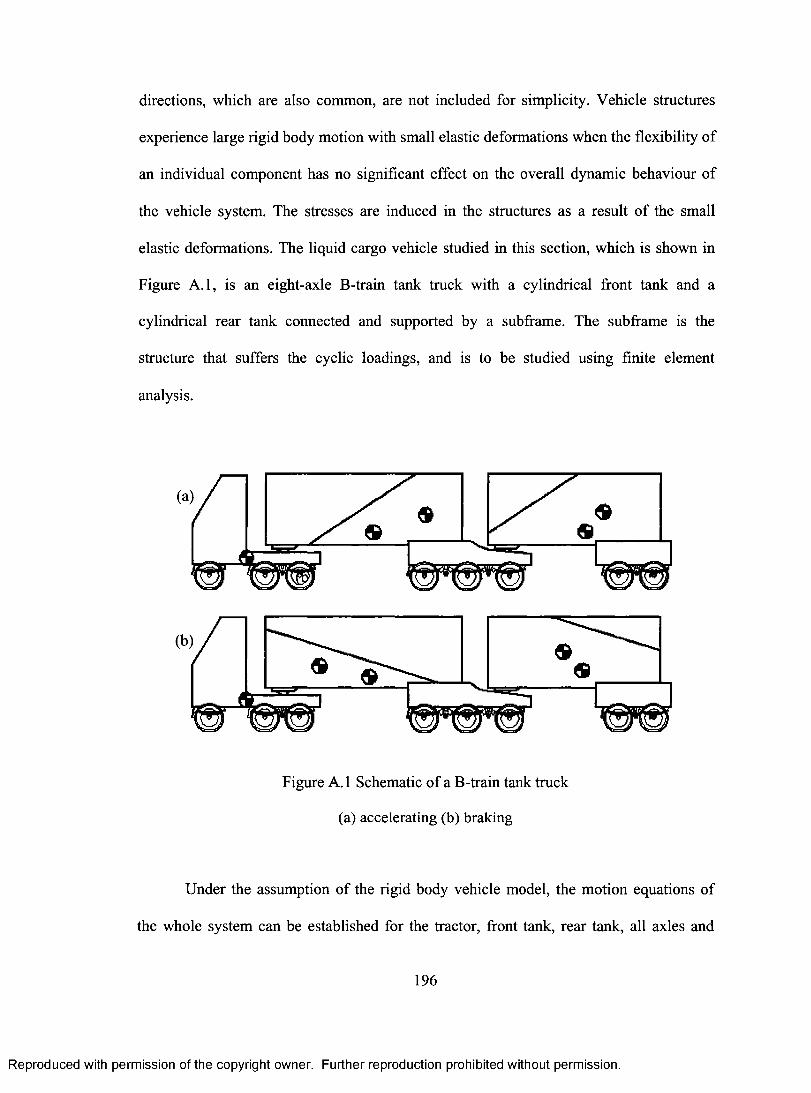
directions, which are also common, are not included for simplicity. Vehicle structures
experience large rigid body motion with small elastic deformations when the flexibility of
an individual component has no significant effect on the overall dynamic behaviour of
the vehicle system. The stresses are induced in the structures as a result of the small
elastic deformations. The liquid cargo vehicle studied in this section, which is shown in
Figure A.1, is an eight-axle B-train tank truck with a cylindrical front tank and a
cylindrical rear tank connected and supported by a subframe. The subframe is the
structure that suffers the cyclic loadings, and is to be studied using finite element
analysis.
Figure A.1 Schematic of a B-train tank truck
(a) accelerating (b) braking
Under the assumption of the rigid body vehicle model, the motion equations of
the whole system can be established for the tractor, front tank, rear tank, all axles and
196
Reproduced with permission of the copyright owner. Further reproduction prohibited without permission.
directions, which are also common, are not included for simplicity. Vehicle structures
experience large rigid body motion with small elastic deformations when the flexibility of
an individual component has no significant effect on the overall dynamic behaviour of
the vehicle system. The stresses are induced in the structures as a result o f the small
elastic deformations. The liquid cargo vehicle studied in this section, which is shown in
Figure A .l, is an eight-axle B-train tank truck with a cylindrical front tank and a
cylindrical rear tank connected and supported by a subframe. The subframe is the
structure that suffers the cyclic loadings, and is to be studied using finite element
analysis.
Under the assumption of the rigid body vehicle model, the motion equations of
the whole system can be established for the tractor, front tank, rear tank, all axles and
(a;
Figure A .l Schematic o f a B-train tank truck
(a) accelerating (b) braking
196
Reproduced with permission of the copyright owner. Further reproduction prohibited without permission.
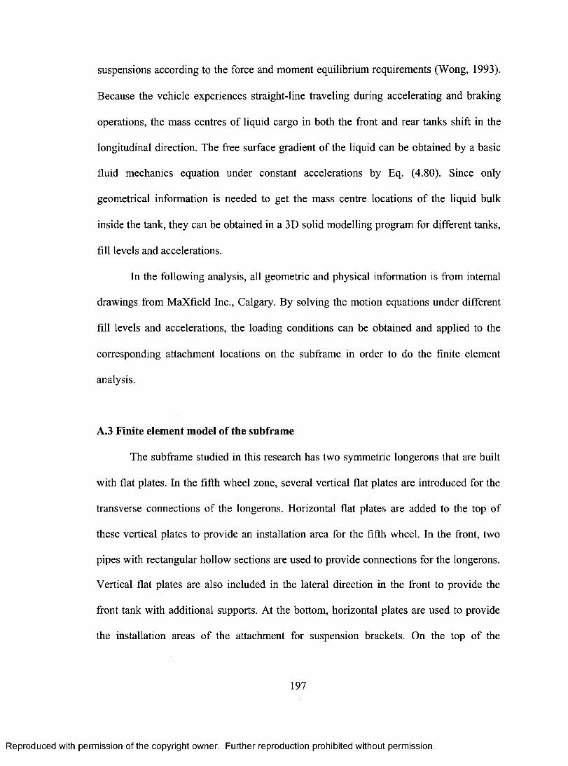
suspensions according to the force and moment equilibrium requirements (Wong, 1993).
Because the vehicle experiences straight-line traveling during accelerating and braking
operations, the mass centres of liquid cargo in both the front and rear tanks shift in the
longitudinal direction. The free surface gradient of the liquid can be obtained by a basic
fluid mechanics equation under constant accelerations by Eq. (4.80). Since only
geometrical information is needed to get the mass centre locations of the liquid bulk
inside the tank, they can be obtained in a 3D solid modelling program for different tanks,
fill levels and accelerations.
In the following analysis, all geometric and physical information is from internal
drawings from MaXfield Inc., Calgary. By solving the motion equations under different
fill levels and accelerations, the loading conditions can be obtained and applied to the
corresponding attachment locations on the subframe in order to do the finite element
analysis.
A.3 Finite element model of the subframe
The subframe studied in this research has two symmetric longerons that are built
with flat plates. In the fifth wheel zone, several vertical flat plates are introduced for the
transverse connections of the longerons. Horizontal flat plates are added to the top of
these vertical plates to provide an installation area for the fifth wheel. In the front, two
pipes with rectangular hollow sections are used to provide connections for the longerons.
Vertical flat plates are also included in the lateral direction in the front to provide the
front tank with additional supports. At the bottom, horizontal plates are used to provide
the installation areas of the attachment for suspension brackets. On the top of the
197
Reproduced with permission of the copyright owner. Further reproduction prohibited without permission.
suspensions according to the force and moment equilibrium requirements (Wong, 1993).
Because the vehicle experiences straight-line traveling during accelerating and braking
operations, the mass centres o f liquid cargo in both the front and rear tanks shift in the
longitudinal direction. The free surface gradient of the liquid can be obtained by a basic
fluid mechanics equation under constant accelerations by Eq. (4.80). Since only
geometrical information is needed to get the mass centre locations o f the liquid bulk
inside the tank, they can be obtained in a 3D solid modelling program for different tanks,
fill levels and accelerations.
In the following analysis, all geometric and physical information is from internal
drawings from MaXfield Inc., Calgary. By solving the motion equations under different
fill levels and accelerations, the loading conditions can be obtained and applied to the
corresponding attachment locations on the subframe in order to do the finite element
analysis.
A.3 Finite element model of the subframe
The subframe studied in this research has two symmetric longerons that are built
with flat plates. In the fifth wheel zone, several vertical flat plates are introduced for the
transverse connections o f the longerons. Horizontal flat plates are added to the top of
these vertical plates to provide an installation area for the fifth wheel. In the front, two
pipes with rectangular hollow sections are used to provide connections for the longerons.
Vertical flat plates are also included in the lateral direction in the front to provide the
front tank with additional supports. At the bottom, horizontal plates are used to provide
the installation areas of the attachment for suspension brackets. On the top of the
197
Reproduced with permission of the copyright owner. Further reproduction prohibited without permission.
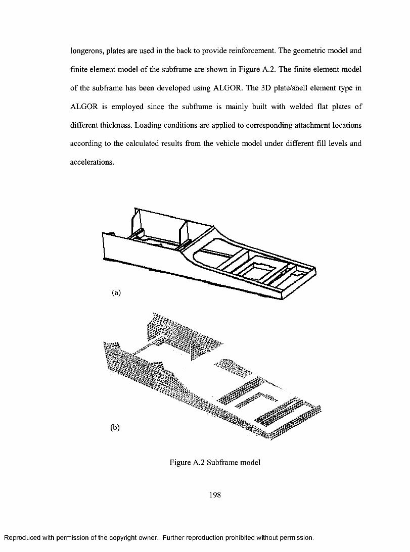
longerons, plates are used in the back to provide reinforcement. The geometric model and
finite element model of the subframe are shown in Figure A.2. The finite element model
of the subframe has been developed using ALGOR. The 3D plate/shell element type in
ALGOR is employed since the subframe is mainly built with welded flat plates of
different thickness. Loading conditions are applied to corresponding attachment locations
according to the calculated results from the vehicle model under different fill levels and
accelerations.
0/
(b)
Figure A.2 Subframe model
198
Reproduced with permission of the copyright owner. Further reproduction prohibited without permission.
longerons, plates are used in the back to provide reinforcement. The geometric model and
finite element model o f the subframe are shown in Figure A. 2. The finite element model
o f the subframe has been developed using ALGOR. The 3D plate/shell element type in
ALGOR is employed since the subframe is mainly built with welded flat plates of
different thickness. Loading conditions are applied to corresponding attachment locations
according to the calculated results from the vehicle model under different fill levels and
accelerations.
Figure A. 2 Subframe model
Reproduced with permission of the copyright owner. Further reproduction prohibited without permission.
(a) geometric model (b) finite element model
A.4 Results and discussion
Figure A.3 shows the load shift for different accelerations when the fill level is
30% in the front tank and 70% in the rear tank. As shown in the figure, when the vehicle
is accelerating, as the acceleration increases (indicated by the arrow), the centre of mass
in the front tank moves closer to the front part of the subframe, and the centre of mass in
the rear tank moves away from the rear part of the subframe. The load shift in the
longitudinal direction is much larger than that in the vertical direction, due to the
geometric shape of the tanks. Also, the load shifts at low fill levels are much larger than
at high fill levels. For a fully filled tank, no load shift will occur. The influence of liquid
motion does not exist for this situation. The load shifts for the same conditions under
braking are shown in Figure A.4. When the vehicle is braking, as the acceleration
increases, the centre of mass in the front tank moves away from the front part of the
subframe and the centre of mass in the rear tank moves closer to the rear part of the
subframe.
Figures A.5 and A.6 show the loads at the hitch point in both longitudinal and
vertical directions during accelerating and braking. The force in the longitudinal direction
increases with the increase in the acceleration and fill level. The negative sign means that
the force in the longitudinal direction is in the opposite direction when braking. The
increase is larger at a high fill level and acceleration. The vertical force increases with the
increase in total payload. During acceleration, the vertical force decreases with the
increase in acceleration because the cargo moves away from the fifth wheel zone. During
braking, the vertical force increases with the increase in acceleration because the load
199
Reproduced with permission of the copyright owner. Further reproduction prohibited without permission.
(a) geometric model (b) finite element model
A.4 Results and discussion
Figure A.3 shows the load shift for different accelerations when the fill level is
30% in the front tank and 70% in the rear tank. As shown in the figure, when the vehicle
is accelerating, as the acceleration increases (indicated by the arrow), the centre o f mass
in the front tank moves closer to the front part o f the subframe, and the centre o f mass in
the rear tank moves away from the rear part o f the subframe. The load shift in the
longitudinal direction is much larger than that in the vertical direction, due to the
geometric shape o f the tanks. Also, the load shifts at low fill levels are much larger than
at high fill levels. For a fully filled tank, no load shift will occur. The influence o f liquid
motion does not exist for this situation. The load shifts for the same conditions under
braking are shown in Figure A.4. When the vehicle is braking, as the acceleration
increases, the centre o f mass in the front tank moves away from the front part o f the
subframe and the centre of mass in the rear tank moves closer to the rear part of the
subframe.
Figures A.5 and A.6 show the loads at the hitch point in both longitudinal and
vertical directions during accelerating and braking. The force in the longitudinal direction
increases with the increase in the acceleration and fill level. The negative sign means that
the force in the longitudinal direction is in the opposite direction when braking. The
increase is larger at a high fill level and acceleration. The vertical force increases with the
increase in total payload. During acceleration, the vertical force decreases with the
increase in acceleration because the cargo moves away from the fifth wheel zone. During
braking, the vertical force increases with the increase in acceleration because the load
199
Reproduced with permission of the copyright owner. Further reproduction prohibited without permission.
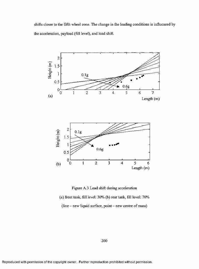
shifts closer to the fifth wheel zone. The change in the loading conditions is influenced by
the acceleration, payload (fill level), and load shift.
1
1
2 3 4 5 6 7
Length (m)
0.6g
2 3 4 5 6 Length (m)
Figure A.3 Load shift during acceleration
(a) front tank, fill level: 30% (b) rear tank, fill level: 70%
(line — new liquid surface, point — new centre of mass)
200
Reproduced with permission of the copyright owner. Further reproduction prohibited without permission.
shifts closer to the fifth wheel zone. The change in the loading conditions is influenced by
the acceleration, payload (fill level), and load shift.
xi.SP'5
(a)
2
1.5
1 O.lg
0.50.6g
03 5 6 70 1 2 4
Length (m)
O.lgS
• • •
0.6g0.5
(b)Length (m)
Figure A.3 Load shift during acceleration
(a) front tank, fill level: 30% (b) rear tank, fill level: 70%
(line - new liquid surface, point - new centre o f mass)
200
Reproduced with permission of the copyright owner. Further reproduction prohibited without permission.
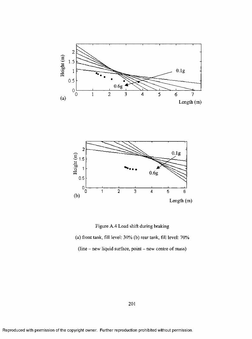
2
1.5 an
"U 1
0.5
0 0
(a) 1 2 3 4 5 6 7
Length (m)
Length (m)
Figure A.4 Load shift during braking
(a) front tank, fill level: 30% (b) rear tank, fill level: 70%
(line — new liquid surface, point — new centre of mass)
201
Reproduced with permission of the copyright owner. Further reproduction prohibited without permission.
2
1 .5
O.lg1
0 . 5
0.6g0
0 1 2 3 4 5 6 7
Length (m)
O.lg
0.6g0.5
(b)Length (m)
Figure A.4 Load shift during braking
(a) front tank, fill level: 30% (b) rear tank, fill level: 70%
(line - new liquid surface, point - new centre o f mass)
201
Reproduced with permission of the copyright owner. Further reproduction prohibited without permission.
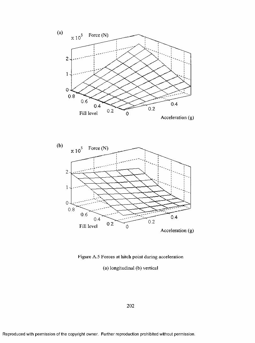
(a)
(b)
0
0.8 0.6
0.4
Fill level 0.2
0
0.8 0.6
0.4
Fill level
x 105 Force (N)
x 105 Force (N)
-meL_M._•mW-111L11111‘.I N_ a.-1116.1.6.‘1W
0.4
e---___ --- '
0.2
0.2 0.4
Acceleration (g)
0.2
Acceleration (g)
Figure A.5 Forces at hitch point during acceleration
(a) longitudinal (b) vertical
202
Reproduced with permission of the copyright owner. Further reproduction prohibited without permission.
(a) 5 Force (N)
0.80.6
0.4Fill level 0 2
0.40.2
Acceleration (g)
(b) .5 Force (N)
Fill level 0 2 0Acceleration (g)
Figure A. 5 Forces at hitch point during acceleration
(a) longitudinal (b) vertical
202
Reproduced with permission of the copyright owner. Further reproduction prohibited without permission.
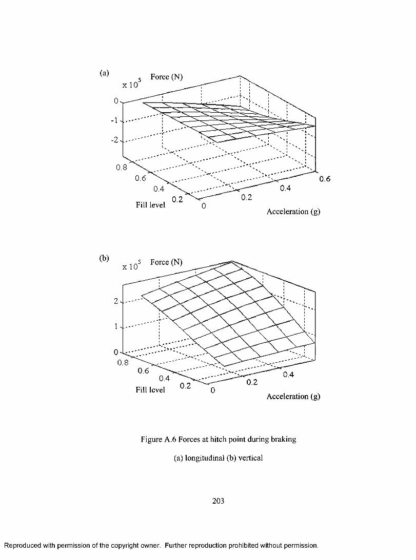
(a)
(b)
x 1 0
0.8
0 0.8
0.6 0.4
Fill level 0.2
5 Force (N)
0.6 0.4
Fill level 0.2
x 105 Force (N)
0.2
0.6 0.4
Acceleration (g)
Acceleration (g)
Figure A.6 Forces at hitch point during braking
(a) longitudinal (b) vertical
203
Reproduced with permission of the copyright owner. Further reproduction prohibited without permission.
(a) Force (N)
0.2Fill level 0
Acceleration (g)
(b) . a5 Force (N) x 10 v ’
0.80.6
0.4Fill level ^
0.40.2
Acceleration (g)
Figure A.6 Forces at hitch point during braking
(a) longitudinal (b) vertical
203
Reproduced with permission of the copyright owner. Further reproduction prohibited without permission.
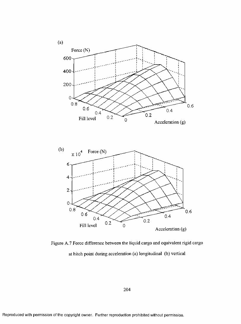
(a)
Force (N)
600
400
200
0 0.8
0.6 0.4
Fill level
(b) x 10
4 Force (N)
0.8 0.6
0.4
Fill level 0' 2.
0.2
0.6 0.4
0.2
Acceleration (g)
0.2
0.6 0.4
Acceleration (g)
Figure A.7 Force difference between the liquid cargo and equivalent rigid cargo
at hitch point during acceleration (a) longitudinal (b) vertical
204
Reproduced with permission of the copyright owner. Further reproduction prohibited without permission.
(a)
Force (N)
600
400
200
0.80.6 0.40.4 0.20.2Fill level
Acceleration (g)
(b) 1 Force (N) x 10
0.8 0.60.6 / 0.4 <
Fill level
0.40.2
Acceleration (g)
Figure A.7 Force difference between the liquid cargo and equivalent rigid cargo
at hitch point during acceleration (a) longitudinal (b) vertical
204
Reproduced with permission of the copyright owner. Further reproduction prohibited without permission.
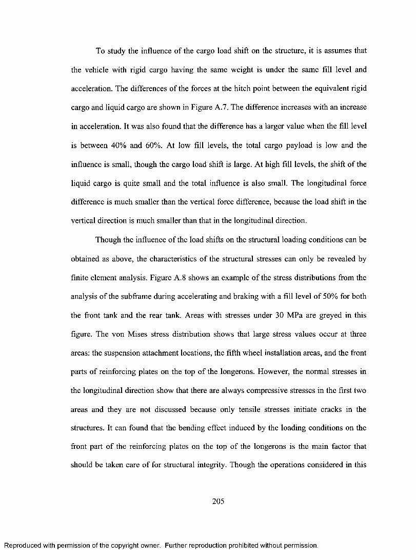
To study the influence of the cargo load shift on the structure, it is assumes that
the vehicle with rigid cargo having the same weight is under the same fill level and
acceleration. The differences of the forces at the hitch point between the equivalent rigid
cargo and liquid cargo are shown in Figure A.7. The difference increases with an increase
in acceleration. It was also found that the difference has a larger value when the fill level
is between 40% and 60%. At low fill levels, the total cargo payload is low and the
influence is small, though the cargo load shift is large. At high fill levels, the shift of the
liquid cargo is quite small and the total influence is also small. The longitudinal force
difference is much smaller than the vertical force difference, because the load shift in the
vertical direction is much smaller than that in the longitudinal direction.
Though the influence of the load shifts on the structural loading conditions can be
obtained as above, the characteristics of the structural stresses can only be revealed by
finite element analysis. Figure A.8 shows an example of the stress distributions from the
analysis of the subframe during accelerating and braking with a fill level of 50% for both
the front tank and the rear tank. Areas with stresses under 30 MPa are greyed in this
figure. The von Mises stress distribution shows that large stress values occur at three
areas: the suspension attachment locations, the fifth wheel installation areas, and the front
parts of reinforcing plates on the top of the longerons. However, the normal stresses in
the longitudinal direction show that there are always compressive stresses in the first two
areas and they are not discussed because only tensile stresses initiate cracks in the
structures. It can found that the bending effect induced by the loading conditions on the
front part of the reinforcing plates on the top of the longerons is the main factor that
should be taken care of for structural integrity. Though the operations considered in this
205
Reproduced with permission of the copyright owner. Further reproduction prohibited without permission.
To study the influence o f the cargo load shift on the structure, it is assumes that
the vehicle with rigid cargo having the same weight is under the same fill level and
acceleration. The differences of the forces at the hitch point between the equivalent rigid
cargo and liquid cargo are shown in Figure A.7. The difference increases with an increase
in acceleration. It was also found that the difference has a larger value when the fill level
is between 40% and 60%. At low fill levels, the total cargo payload is low and the
influence is small, though the cargo load shift is large. At high fill levels, the shift of the
liquid cargo is quite small and the total influence is also small. The longitudinal force
difference is much smaller than the vertical force difference, because the load shift in the
vertical direction is much smaller than that in the longitudinal direction.
Though the influence o f the load shifts on the structural loading conditions can be
obtained as above, the characteristics o f the structural stresses can only be revealed by
finite element analysis. Figure A.8 shows an example o f the stress distributions from the
analysis o f the subframe during accelerating and braking with a fill level o f 50% for both
the front tank and the rear tank. Areas with stresses under 30 MPa are greyed in this
figure. The von Mises stress distribution shows that large stress values occur at three
areas: the suspension attachment locations, the fifth wheel installation areas, and the front
parts o f reinforcing plates on the top o f the longerons. However, the normal stresses in
the longitudinal direction show that there are always compressive stresses in the first two
areas and they are not discussed because only tensile stresses initiate cracks in the
structures. It can found that the bending effect induced by the loading conditions on the
front part of the reinforcing plates on the top of the longerons is the main factor that
should be taken care of for structural integrity. Though the operations considered in this
205
Reproduced with permission of the copyright owner. Further reproduction prohibited without permission.
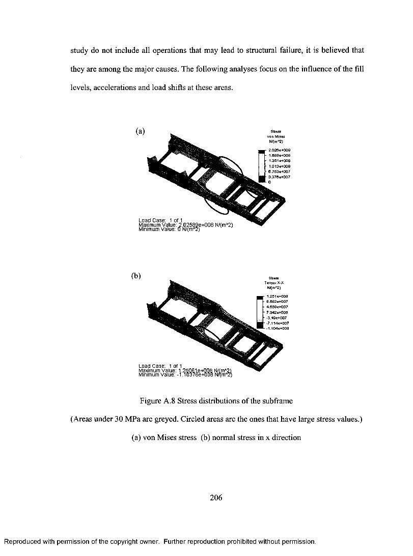
study do not include all operations that may lead to structural failure, it is believed that
they are among the major causes. The following analyses focus on the influence of the fill
levels, accelerations and load shifts at these areas.
(a)
Load Case: 1 of 1 Maximum Value: 2.02589e+008 N/(mA2) Minimum Value: 0 N/(mA2)
(b)
Load Case: 1 of 1 Maximum Value: 1.25061e+008 N/LmA2i Minimum Value: -1.10376e+008 I\1/(mAz)
Stress von Mines
W(rn^2)
2.028e+008 :
1.688e+008 1.351 e+005
1.013 e+008
6.753e+007 3.3780+007 0
Stress Tensor X-X
Nkrn^2)
1.251e+008 8.582e+007
4.858 e+007
7.342e+006 -3.19e+007
-7.114e+007 -1.104e+008
Figure A.8 Stress distributions of the subframe
(Areas under 30 MPa are greyed. Circled areas are the ones that have large stress values.)
(a) von Mises stress (b) normal stress in x direction
206
Reproduced with permission of the copyright owner. Further reproduction prohibited without permission.
study do not include all operations that may lead to structural failure, it is believed that
they are among the major causes. The following analyses focus on the influence o f the fill
levels, accelerations and load shifts at these areas.
L oad C ase : 1 of 1Maximum Value: 2 .0 2 5 8 9 e+ 0 0 8 N/(mA2) Minimum Value: 0 N/(mA2)
S t r e s s
v o n M is e s
N / ( m A2 )
2 . 0 2 6 e + 0 0 8
1 . 6 8 8 * + 0 0 8
1 . 3 5 1 * + 0 0 8
1 . 0 1 3 e + 0 0 8
6 . 7 5 3 e + 0 0 7
3 . 3 7 6 « + 0 0 7
0
(b)T e n s o r X - X
N/fmA2)
1 . 2 5 1 e + 0 0 8
8 , 5 8 2 e + 0 0 7
4 . 6 5 8 e + 0 0 7
7 . 3 4 2 e + 0 0 6
• 3 . 1 9 6 + 0 0 7
- 7 . 1 1 4 e + 0 0 7
- 1 . 1 0 4 e + 0 0 8
Load C ase: 1 of 1Maximum Value: 1.25061 e+008 IM/(mA2 Minimum Value: - 1 .10376e+ 008 W
Figure A.8 Stress distributions of the subframe
(Areas under 30 MPa are greyed. Circled areas are the ones that have large stress values.)
(a) von Mises stress (b) normal stress in x direction
206
Reproduced with permission of the copyright owner. Further reproduction prohibited without permission.
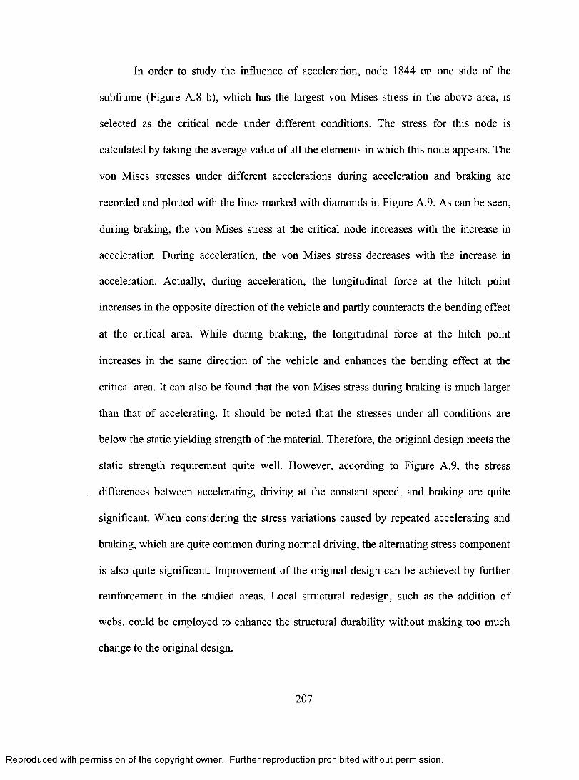
In order to study the influence of acceleration, node 1844 on one side of the
subframe (Figure A.8 b), which has the largest von Mises stress in the above area, is
selected as the critical node under different conditions. The stress for this node is
calculated by taking the average value of all the elements in which this node appears. The
von Mises stresses under different accelerations during acceleration and braking are
recorded and plotted with the lines marked with diamonds in Figure A.9. As can be seen,
during braking, the von Mises stress at the critical node increases with the increase in
acceleration. During acceleration, the von Mises stress decreases with the increase in
acceleration. Actually, during acceleration, the longitudinal force at the hitch point
increases in the opposite direction of the vehicle and partly counteracts the bending effect
at the critical area. While during braking, the longitudinal force at the hitch point
increases in the same direction of the vehicle and enhances the bending effect at the
critical area. It can also be found that the von Mises stress during braking is much larger
than that of accelerating. It should be noted that the stresses under all conditions are
below the static yielding strength of the material. Therefore, the original design meets the
static strength requirement quite well. However, according to Figure A.9, the stress
differences between accelerating, driving at the constant speed, and braking are quite
significant. When considering the stress variations caused by repeated accelerating and
braking, which are quite common during normal driving, the alternating stress component
is also quite significant. Improvement of the original design can be achieved by further
reinforcement in the studied areas. Local structural redesign, such as the addition of
webs, could be employed to enhance the structural durability without making too much
change to the original design.
207
Reproduced with permission of the copyright owner. Further reproduction prohibited without permission.
In order to study the influence of acceleration, node 1844 on one side of the
subframe (Figure A.8 b), which has the largest von Mises stress in the above area, is
selected as the critical node under different conditions. The stress for this node is
calculated by taking the average value of all the elements in which this node appears. The
von Mises stresses under different accelerations during acceleration and braking are
recorded and plotted with the lines marked with diamonds in Figure A.9. As can be seen,
during braking, the von Mises stress at the critical node increases with the increase in
acceleration. During acceleration, the von Mises stress decreases with the increase in
acceleration. Actually, during acceleration, the longitudinal force at the hitch point
increases in the opposite direction o f the vehicle and partly counteracts the bending effect
at the critical area. While during braking, the longitudinal force at the hitch point
increases in the same direction o f the vehicle and enhances the bending effect at the
critical area. It can also be found that the von Mises stress during braking is much larger
than that o f accelerating. It should be noted that the stresses under all conditions are
below the static yielding strength o f the material. Therefore, the original design meets the
static strength requirement quite well. However, according to Figure A.9, the stress
differences between accelerating, driving at the constant speed, and braking are quite
significant. When considering the stress variations caused by repeated accelerating and
braking, which are quite common during normal driving, the alternating stress component
is also quite significant. Improvement o f the original design can be achieved by further
reinforcement in the studied areas. Local structural redesign, such as the addition of
webs, could be employed to enhance the structural durability without making too much
change to the original design.
207
Reproduced with permission of the copyright owner. Further reproduction prohibited without permission.
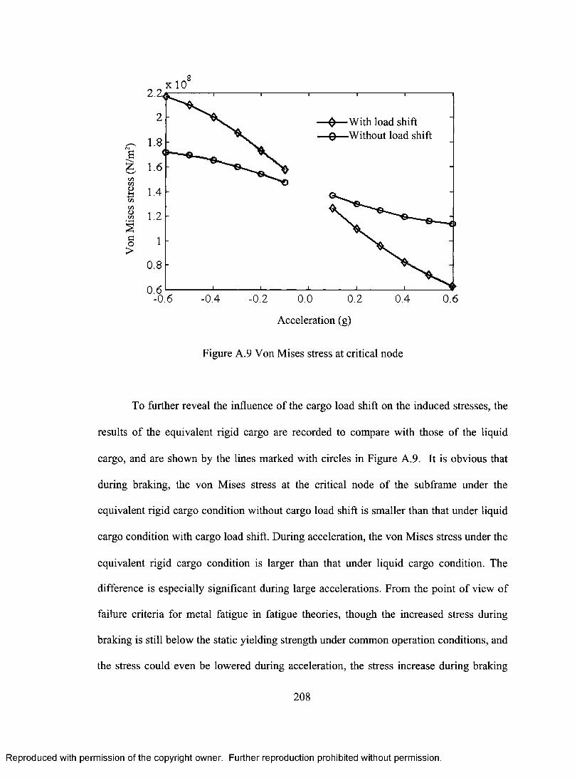
Von
Mis
es s
tres
s (N
/m2)
X 10$ 2.
2
1.8
1.6
1.4
1.2
1
0.8
0.6 -0.6
—With load shift $Without load shift
-0.4 -0.2 0.0 0.2
Acceleration (g)
0.4
Figure A.9 Von Mises stress at critical node
0.6
To further reveal the influence of the cargo load shift on the induced stresses, the
results of the equivalent rigid cargo are recorded to compare with those of the liquid
cargo, and are shown by the lines marked with circles in Figure A.9. It is obvious that
during braking, the von Mises stress at the critical node of the subframe under the
equivalent rigid cargo condition without cargo load shift is smaller than that under liquid
cargo condition with cargo load shift. During acceleration, the von Mises stress under the
equivalent rigid cargo condition is larger than that under liquid cargo condition. The
difference is especially significant during large accelerations. From the point of view of
failure criteria for metal fatigue in fatigue theories, though the increased stress during
braking is still below the static yielding strength under common operation conditions, and
the stress could even be lowered during acceleration, the stress increase during braking
208
Reproduced with permission of the copyright owner. Further reproduction prohibited without permission.
■0— With load shift ■Q— Without load shift
£z
0.8
0.6 L -0.6 -0.4 - 0.2 0.0 0.2 0.4 0.6
Acceleration (g)
Figure A.9 Von Mises stress at critical node
To further reveal the influence of the cargo load shift on the induced stresses, the
results o f the equivalent rigid cargo are recorded to compare with those of the liquid
cargo, and are shown by the lines marked with circles in Figure A.9. It is obvious that
during braking, the von Mises stress at the critical node of the subframe under the
equivalent rigid cargo condition without cargo load shift is smaller than that under liquid
cargo condition with cargo load shift. During acceleration, the von Mises stress under the
equivalent rigid cargo condition is larger than that under liquid cargo condition. The
difference is especially significant during large accelerations. From the point of view of
failure criteria for metal fatigue in fatigue theories, though the increased stress during
braking is still below the static yielding strength under common operation conditions, and
the stress could even be lowered during acceleration, the stress increase during braking
208
Reproduced with permission of the copyright owner. Further reproduction prohibited without permission.
and stress decrease during acceleration caused by the cargo load shift are extremely
harmful to the fatigue life of the structures. Under frequent acceleration and braking, the
combined effect of the acceleration and cargo load shift makes the alternating stress
component, which is the most important factor in determining the number of cycles of
load the material can withstand before fracture, much larger than that of the subframe
subjected only to acceleration. Therefore, the cargo load shift exerts an additional and
significant effect on the cyclic loadings on the subframe. It is detrimental to the structural
durability.
A.5 Summary
In this section, the influence of the accelerating and braking operations on the
structural strength of a B-train tank truck subframe has been investigated. The loading
conditions on an existing design of the subframe have been obtained using the pitch plane
vehicle model under constant accelerations. Finite element analysis of the subframe has
been implemented. The influence of the acceleration, fill level, and cargo load shift has
been studied. The analysis results show that the critical area is located on the front part of
the reinforcing plates on the top of the longerons, and that structural failure is mainly
caused by the bending effect at this area. Improvement of the existing design could be
achieved by further reinforcement at the studied locations. In addition to the inertia effect
induced by accelerations, the cargo load shift exerts an extra effect on the cyclic loadings
on the subframe. It has a detrimental influence on the structural durability.
As shown in Chapter 3 and Chapter 4, the results of the mass centre model only
show the mean values of the oscillatory forces and moments caused by the liquid motion
209
Reproduced with permission of the copyright owner. Further reproduction prohibited without permission.
and stress decrease during acceleration caused by the cargo load shift are extremely
harmful to the fatigue life of the structures. Under frequent acceleration and braking, the
combined effect o f the acceleration and cargo load shift makes the alternating stress
component, which is the most important factor in determining the number o f cycles of
load the material can withstand before fracture, much larger than that o f the subframe
subjected only to acceleration. Therefore, the cargo load shift exerts an additional and
significant effect on the cyclic loadings on the subframe. It is detrimental to the structural
durability.
A.5 Summary
In this section, the influence o f the accelerating and braking operations on the
structural strength of a B-train tank truck subframe has been investigated. The loading
conditions on an existing design of the subframe have been obtained using the pitch plane
vehicle model under constant accelerations. Finite element analysis o f the subframe has
been implemented. The influence of the acceleration, fill level, and cargo load shift has
been studied. The analysis results show that the critical area is located on the front part of
the reinforcing plates on the top o f the longerons, and that structural failure is mainly
caused by the bending effect at this area. Improvement of the existing design could be
achieved by further reinforcement at the studied locations. In addition to the inertia effect
induced by accelerations, the cargo load shift exerts an extra effect on the cyclic loadings
on the subframe. It has a detrimental influence on the structural durability.
As shown in Chapter 3 and Chapter 4, the results of the mass centre model only
show the mean values of the oscillatory forces and moments caused by the liquid motion
209
Reproduced with permission of the copyright owner. Further reproduction prohibited without permission.
immediately after the application of the acceleration. When the tank is subjected to a
suddenly applied acceleration, the oscillatory liquid motion causes oscillatory forces and
moments of considerable magnitudes, which are not only harmful to vehicle stability and
controllability, but also exert direct cyclical loadings on the supporting structures. The
stress analysis based on these cyclical loadings is very important for the fatigue life of
tank vehicle structures. To fully reveal the relationship between the liquid motion and the
structural strength and fatigue life, further studies are definitely necessary in order to
include the influence of the dynamic liquid behaviour under different operation
conditions on vehicle structures. With the integration of the method developed in the
previous chapters into dynamic vehicle models, structural analysis can be continued
based on the established finite element model and the loading conditions of the liquid-
vehicle-structure model.
210
Reproduced with permission of the copyright owner. Further reproduction prohibited without permission.
immediately after the application of the acceleration. When the tank is subjected to a
suddenly applied acceleration, the oscillatory liquid motion causes oscillatory forces and
moments o f considerable magnitudes, which are not only harmful to vehicle stability and
controllability, but also exert direct cyclical loadings on the supporting structures. The
stress analysis based on these cyclical loadings is very important for the fatigue life of
tank vehicle structures. To fully reveal the relationship between the liquid motion and the
structural strength and fatigue life, further studies are definitely necessary in order to
include the influence of the dynamic liquid behaviour under different operation
conditions on vehicle structures. With the integration of the method developed in the
previous chapters into dynamic vehicle models, structural analysis can be continued
based on the established finite element model and the loading conditions o f the liquid-
vehicle-structure model.
210
Reproduced with permission of the copyright owner. Further reproduction prohibited without permission.