DAPL IIR Filter Module Manual - Microstar Laboratories

DAPL IIR Filter Module Manual

DAPL IIR Filter Module applications and command reference

Version 1.00

Microstar Laboratories, Inc.

This manual contains proprietary information which is protected by copyright. All rights are reserved. No part of this manual may be photocopied, reproduced, or translated to another language without prior written consent of Microstar Laboratories, Inc.

Copyright © 2000-2001 Microstar Laboratories, Inc. 2265 116th Avenue N.E. Bellevue, WA 98004 Tel: (425) 453-2345 Fax: (425) 453-3199 http://www.mstarlabs.com

Microstar Laboratories, DAPcell, Data Acquisition Processor, DAP, DAPL, and DAPview are trademarks of Microstar Laboratories, Inc.

Microstar Laboratories requires express written approval from its President if any Microstar Laboratories products are to be used in or with systems, devices, or applications in which failure can be expected to endanger human life.

Microsoft, MS, and MS-DOS are registered trademarks of Microsoft Corporation. Windows is a trademark of Microsoft Corporation. IBM is a registered trademark of International Business Machines Corporation. Intel is a registered trademark of Intel Corporation. Novell and NetWare are registered trademarks of Novell, Inc. Other brand and product names are trademarks or registered trademarks of their respective holders.

Part Number MSDAPLIFMM100

Contents iii

Contents

1. Digital and Analog Filtering................................................................................................. 1 Why Filter?........................................................................................................................ 1 Filters: Analog and Digital ................................................................................................ 2 Digital Filters: Finite or Infinite Response ........................................................................ 3

FIR Filtering................................................................................................................ 3 IIR Filtering................................................................................................................. 4

2. IIR Filter Families................................................................................................................. 7 Butterworth Filters............................................................................................................. 7 Bessel Filters ..................................................................................................................... 8 Chebyshev Filters ............................................................................................................ 10 Inverse Chebyshev Filters................................................................................................ 12 Elliptic Filters .................................................................................................................. 14

3. How Good Are The Filter Designs? ................................................................................... 21 Obtaining Detailed Design Information........................................................................... 25

4. IIR Filter Parameters.......................................................................................................... 27 Filter Order ...................................................................................................................... 27 Cutoff Frequency............................................................................................................. 27 Passband Ripple .............................................................................................................. 28 Stopband Rejection.......................................................................................................... 29

5. Application Examples ......................................................................................................... 31 Filter Families.................................................................................................................. 31

6. IIR Filter Module Command Reference............................................................................ 35 BESSEL........................................................................................................................... 36 BUTTERWORTH ........................................................................................................... 39 CHEBYINV .................................................................................................................... 42 CHEBYSHEV ................................................................................................................. 45 ELLIPTIC........................................................................................................................ 49 FIRFILTER ..................................................................................................................... 52

Index......................................................................................................................................... 53

Digital and Analog Filtering 1

1. Digital and Analog Filtering

This section provides an overview of filtering, the role of digital signal processing in filtering, the FIR and IIR types of digital filters, and how to select an appropriate filter type for an application.

Why Filter?

The basic reason for filtering is because an application requires it! Applications apply filtering to discriminate between different bands of frequencies, responding to some, and suppressing others. Examples include:

• Eliminating interference from power-line frequencies • Eliminating very low frequency “DC offset drift” from a signal • Selecting characteristic frequencies that contain the best information • Reducing the effects of random measurement noise • Detecting the presence of a special signal tone • Preserving accurate signal samples when using data acquisition equipment (anti-

aliasing)

Filtering technologies were first developed for continuous signals using analog circuit elements, and these technologies are still appropriate and widely used today. However, digital processing is becoming more and more accessible because of rapidly developing digital hardware technologies.

Digital processing requires converting the signals from a continuous waveform into an equivalent representation as a sequence of discrete numerical values. There are two strategies for filtering a signal when doing this:

1. Apply continuous filtering technologies to perform the required filtering as before, then capture digitized samples of the filtered waveforms.

2. Capture digitized samples of the original waveforms prior to filtering, and then apply mathematical operations to the data stream to emulate the effects that an analog filter would provide.

Which approach is better depends on many factors, but two of the most important are configurability and economy. For an application requiring simple filtering on very few signal channels, hardware-based analog technologies are probably the best solution. For applications requiring complex filtering on several channels, where the filtering characteristics might need to be individually adjusted, and where fabrication of

2 Digital and Analog Filtering

hardware-based filters would be too expensive, a software-based digital technology is likely a better choice.

Filters: Analog and Digital

The digital filter families in this package provide the same benefits as their corresponding analog filter families. The correspondence is very close – but not exact. That is the nature of a discrete numerical approximation, highly accurate, but with certain limitations.

The most critical limitation of a sampled signal representation is the Nyquist limit. A sample sequence obtained by capturing data samples at regular time interval T is considered to have “sampling frequency” Fs = 1/T. The Nyquist limit is half of this frequency

Fn = (1/ 2) x Fs

Frequencies above the Nyquist limit cannot be distinguished from frequencies below it in the sampled data. This leads to the phenomenon called “aliasing.” For example, in figure 1 below, the data samples indicated by black dots could result from sampling either the dark curve (below the Nyquist limit) or the light curve (above the Nyquist limit).

Figure 1: Frequencies above and below the Nyquist limit yield indistinguishable data samples.

If both frequencies are present, both contribute to the sample values. Depending on the phase of the two frequency components, the values may add or cancel. This is usually impossible to predict, and definitely impossible to correct after the signal samples have been recorded. The only way to guarantee that irrelevant frequencies above the Nyquist frequency limit do not corrupt measurements of frequencies below


the Nyquist limit is to guarantee that problematic high frequencies are not present when the continuous signal is sampled.

One way to eliminate an aliasing problem is to assume it away. If the high frequencies are random, and the total energy in the noise bands is small, the effects on the samples will be random and small – white noise. On the other hand, if the high frequencies are not random noise, the accurate sampling of a Data Acquisition Processor (or any other high-quality data acquisition device) is guaranteed to exactly produce all of the aliasing artifacts, whether you want them or not. Some people who assumed away interfering signals discovered too late that noise sources were non-random, and the data corruption introduced by aliasing was on the order of plus or minus 100%. Do you feel lucky?

Another approach to avoiding aliasing is to combine the best properties of the digital and analog worlds. A relatively simple passive analog filter can “roll off” or “bypass” all of the very high frequencies, and then the digital sampling can run at a sufficiently high rate – oversampling relative to the rates strictly required to represent the signal – so that aliasing effects in the desired frequency band are negligible.

Given guarantees that aliasing effects from discrete sampling are insignificant, the results of applying a digital filter or an analog filter are virtually identical. A complete anti-aliasing solution as provide by the Microstar Laboratories iDSC products can guarantee alias-free data, but in some cases other means are good enough to avoid aliasing problems.

Digital Filters: Finite or Infinite Response

Having obtained a clean, sampled representation of a signal, and having determined that digital filtering in software provides a good economic solution for the filtering requirements, there remains a choice of how to do the filtering. There are two types of digital filters that can be applied: finite impulse response filtering, or infinite impulse response filtering. This section will briefly compare the two approaches.

FIR Filtering

Finite impulse response (FIR) filtering applies a mathematical operation to a stream of data samples to compute filtered outputs. The most common filters of this class are the “symmetric FIR filters” such as the designs generated by the Microstar Laboratories design program FGEN for Windows and used by the FIRFILTFIRFILTFIRFILTFIRFILTERERERER command built into the DAPL operating system. A finite impulse response filtering operation can be considered a weighted sum of data sample values, with the coefficients of the filter serving as the weighting factors.

4 Digital and Analog Filtering

The symmetry property of symmetric FIR filters comes from using an equal number of data samples before and after a particular position in the data stream. While it is clear that a history of past samples is available for doing this computation, it is less clear how the filter can be applied to future samples! The answer, of course, is that computations must be delayed until those samples are available. This delay can’t be extended forever, so only a finite number of past and future terms can be used in the computation. Consequently, an impulse signal appearing in the input data stream can affect only a finite number of output samples, hence the name finite impulse response filtering.

The quality of FIR-filtered data is excellent. These filters are the basis of the superior performance of the iDSC products. In particular, symmetric FIR filters do not shift different frequencies relative to each other -- technically speaking, the phase shift is proportional to frequency. This means minimal distortion in the signal, preserving all magnitude and relative phase information in the retained frequency band.

FIR filtering also has the advantages of decimating efficiently. If high frequencies are completely removed by filtering, there is no point in retaining a very high sample rate in the data sequence; because much of the data is redundant. The computational load can be reduced by deleting a major portion of the redundant samples, with no loss of accuracy in the representation of the signal.

One cost of FIR filtering is the real-time delay waiting for samples to arrive before filtering operations can be applied. Applications that must respond in real time to information from the filtered signal might experience unacceptable delay times.

IIR Filtering

The alternative approach, called infinite impulse response (IIR) filtering, is supported by the DAPL IIR Filter Module. While a FIR filtering operation is applied to the stream of data samples only, IIR filtering uses data samples and also past history of the filter response for deriving subsequent filtered values. This makes IIR filtering a more general but more complicated kind of filtering. Using past output values establishes a kind of “feedback” resulting in an infinitely decaying response from an impulse disturbance in the data stream, hence the name infinite impulse response filtering.

Whether the response to an impulse is strictly limited in time or converges to zero over an extended period of time makes little difference in practice. What is important is that the IIR filters tend to have natural resonances and decay rates analogous to tuned circuits in an analog filter. This is a definite advantage if the goal is to accurately replicate responses of analog filter families – including all of the phase shifts, for better or worse.


Because the IIR filters generally have no symmetry property, they do not need to wait for input data and can respond quickly to changes in the input data stream.

IIR filters are typically not as useful as FIR filters for decimation applications, because they have no means to reproduce the internal representations of past history if input data is skipped.

IIR filters excel for isolating very low frequencies. To distinguish very low frequencies, a filter must preserve information over a long time interval. The only way to do this with a FIR filter is to use an exceptionally long data history, with corresponding long and costly computations. An IIR filter, on the other hand, retains information about a long period of past history by applying a very slow internal decay rate to information about past outputs. Adjusting these decay coefficients does not affect the structure or complexity of the filter.

One additional special property of IIR filters: they can be designed to have natural resonance frequencies just below the cutoff frequency, sustaining the passband response level, and zeroes of transmission just above the cutoff frequency to force the stopband response to zero. This yields a filter with an exceptionally abrupt “brick wall” cutoff. But there is a cost. The resonant frequencies can cause havoc with passband flatness and phase response.

IIR Filter Families 7

2. IIR Filter Families

This chapter describes the filter families supported by the DAPL IIR Filter Module, comparing their advantages and disadvantages.

After IIR filtering has been chosen for a digital filtering application, the problem of obtaining an optimized IIR filter design for that one application is an advanced mathematical exercise best left to specialists. However, there are some generalized cases for which the design work has already been done. Prominent among these are design methods based on established analog filter families. These techniques map the parameters of an analog filter design into the parameter of an equivalent filter in the discrete sample domain. The method used for doing this is called bilinear mapping with pre-warping. Fortunately, you don’t need to worry about all of the technical details – the hard math is done automatically, and the filters will work exactly as you specify.

Sometimes the choice of filter family is easy. When “The Specification” says that the filter shall be a sixth order Butterworth filter, the decision is already made! Other times, a filter type for best meeting application objectives must be selected.

Butterworth Filters

Butterworth filters have an optimally flat response at the low frequency end of the spectrum, and a frequency response rolloff that drops smoothly toward zero at the high end of the spectrum, with modest phase distortions near the cutoff frequency. However, the passband is not sustained uniformly, and Butterworth filters are famous for a sagging response at higher passband frequencies, with a rather wide passband-to-stopband transition. When a filtering application is only concerned with low frequencies, and there is relatively little energy at the higher frequencies, the wide transition band might be of no consequence, and a Butterworth filter would be a good choice.

The plot below illustrates a typical Butterworth filter characteristic. As the filter order increases, the passband sustains somewhat better, and the asymptotic stopband rolloff gets steeper, but the high frequency rolloff remains rather wide and rounded.

8 IIR Filter Families

Fraction of Nyquist Frequency

0.0 0.1 0.2 0.3 0.4 0.5 0.7 0.8 0.9 1.00.6

0.0

0.1

0.2

0.3

0.5

0.6

0.7

0.8

0.9

1.0

0.4

Figure 2: Butterworth filters of order 3, 6, 9 and 12, showing a narrowing transition band with higher filter order.

Bessel Filters

To avoid waveform distortions and loss of phase information from filter phase shifts not proportional to frequency, a Bessel filter provides the advantage of a highly linear phase response to well into the cutoff region. It is optimal among the families of IIR filters in this respect. However, compared to the Butterworth filters, the magnitude response of the Bessel filter has very little passband flatness. It places all of the emphasis on phase linearity, with very little improvement in filtering magnitude characteristics from the lowest order filters to the highest.


0.0

0.1

0.2

0.3

0.5

0.6

0.7

0.8

0.9

1.0

0.4

0.0


0.1 0.2 0.3 0.4 0.5 0.7 0.8 0.9 1.00.6

Figure 3: Little difference in magnitude response between order 3 and order 18 Bessel filter.

The phase response is shown in Figure 4.

-8.0

-7.0

-5.0

-4.0

-3.0

-2.0

-1.0

0.0

-6.0

0.0


0.1 0.2 0.3 0.4 0.5 0.7 0.8 0.9 1.00.6

Figure 4: Bessel filter phase response for order 3 and order 12.


The higher order filter is seen to have more phase shift (group delay) and its linear phase response band extends further into the stopband region, but in most other respects, the response characteristics are very similar.

Since symmetric FIR filters offer superior passband flatness and guaranteed linear phase response across the entire spectrum, the question might be asked, why bother with Bessel filters? Good question. There are two situations where they can be useful.

1. “The Specification” calls for a Bessel filter.

2. Real-time response is important.

Other than that, consider FIR filters as a preferred alternative.

Chebyshev Filters

When the Butterworth filter family puts its emphasis on absolute flatness at the low-frequency end of the passband, the response suffers at the high-frequency end of the passband. The Chebyshev filter family, on the other hand, guarantees uniform response through the passband. That is, the passband gain sustains at approximately 1.0 from zero frequency to near the cutoff frequency. However, the magnitude is not flat (at 1.0 gain), rather, it has small “ripples.” While that sounds like a major drawback, the ripples are bounded and of uniform magnitude, and can be adjusted to a small enough level that they are insignificant to the application. For example, in audio applications, 0.1 dB variations in frequency response are not considered audible, so a passband ripple of this magnitude might be considered insignificant.

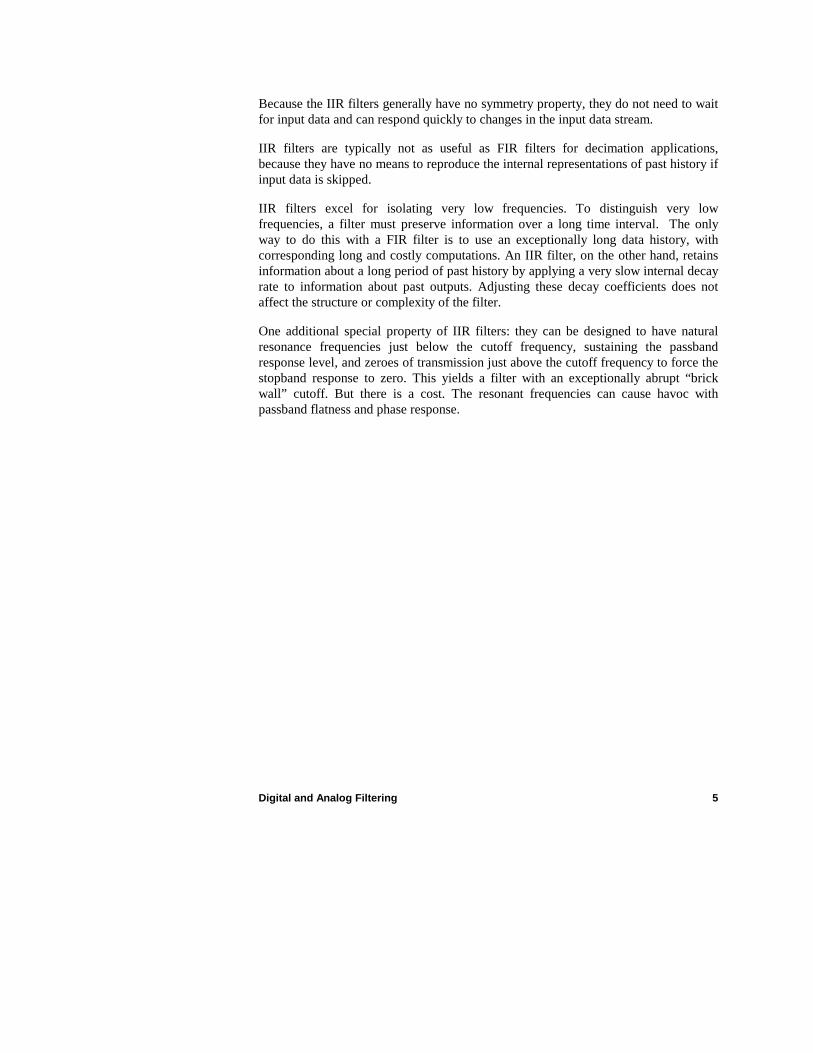
Figure 5 illustrates a seventh-order Chebyshev filter magnitude response for two different ripple parameters, 0.25 dB ripple (about 3%) and 0.01 dB ripple (about 0.1%).


0.0

0.1

0.2

0.3

0.5

0.6

0.7

0.8

0.9

1.0

0.4

0.0


0.1 0.2 0.3 0.4 0.5 0.7 0.8 0.9 1.00.6

Figure 5: Allowing a larger passband ripple in an order-7 Chebyshev filter yields a narrower transition band.

Though the two curves are very similar, the curve with 0.01 dB passband ripple is almost indistinguishable from perfectly flat in the passband, while the curve with 0.25 dB passband ripple has a distinctly narrower transition band.

The magnitude response drops off much more rapidly near the cutoff frequency compared to a Butterworth filter. This means that Chebyshev filters offer good selectivity in distinguishing passband and stopband frequencies. In general, higher filter orders give sharper cutoff transitions. A good approach to specifying a Chebyshev filter is to first establish the allowable ripple magnitude, and then select the lowest filter order that gives an acceptable transition width. The following plot shows the widths of the transition band (from 95% to 5% of the passband magnitude), as a function of the passband ripple and filter order.


0.0

0.1

0.2

0.3

0.5

0.4

0.0001

Passband ripple, dB

0.001 0.01 1.0 10.00.1

12

16

20

10

87 6 5

Figure 6: Chebyshev filter transition width as a function of passband ripple. Transition band width is expressed as a fraction of passband width. Each curve is marked with its filter order.

The poles that sustain the passband response (and cause passband ripple) introduce phase shifts, so the phase response is much less linear than in a Butterworth filter, producing some distortion of wave shapes and loss of phase information.

Inverse Chebyshev Filters

Where the emphasis of the Chebyshev filter is on uniform response in the passband, the emphasis of the Inverse Chebyshev filters is on uniform response in the stopband. All of the filters described so far have the property of increasing stopband rejection with increasing frequency. That is good for the high frequency end of the spectrum, but not so good for the low frequency end, where stopband rejection is often poor near the cutoff frequency. If it is important to guarantee a minimum level of noise rejection everywhere in the stopband, the Inverse Chebyshev filter can be a good choice.

Unlike the Butterworth, Bessel and Chebyshev filter characteristics that only approach zero, the Inverse Chebyshev characteristic reaches and passes through zero producing zeroes of transmission in the stopband. These zeroes keep the stopband response small. By adjusting the relative positions of the zeroes, the worst-case ripple (nonzero stopband response) between transmission zeroes is made uniform and as low as


possible. Like the Chebyshev filter, the ripple magnitude is adjustable, and the response in the stopband can be reduced to insignificance for the purposes of the application. The following diagram illustrates an Inverse Chebyshev response with a stopband rejection of 30 dB, about 3% ripple magnitude, and with stopband rejection of 60 dB, about 0.1% ripple magnitude.

0.0


0.1 0.2 0.3 0.4 0.5 0.7 0.8 0.9 1.00.6

0.0

0.1

0.2

0.3

0.5

0.6

0.7

0.8

0.9

1.0

0.4

Figure 7: 6th order Inverse Chebyshev filters, 30 dB and 60 dB minimum stopband rejection.

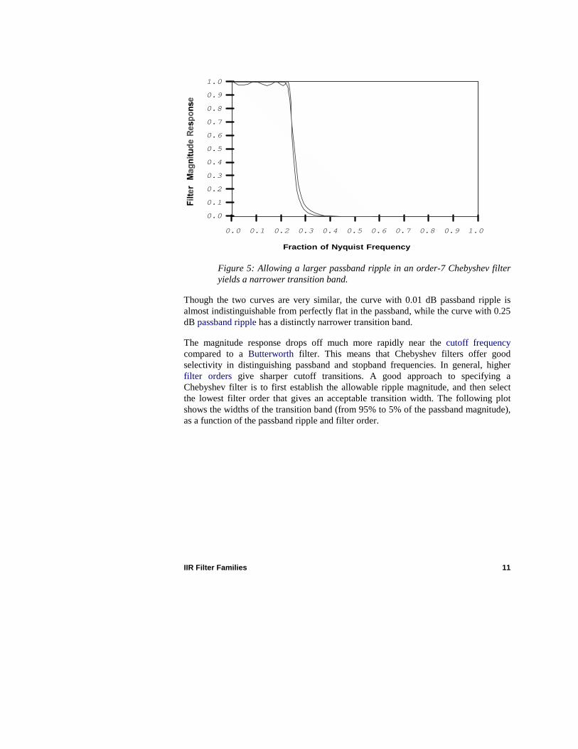
As with the Chebyshev filter, there is a tradeoff between the amount of ripple and the sharpness of the cutoff transition. Because there is less emphasis on enforcing extremely high rejection at the high frequency end of the stopband, the Inverse Chebyshev filter is able to provide a wider passband, still with good flatness at low frequencies similar to a Butterworth filter. The graph in Figure 8 shows the widths of the transition band (from 95% to 5% of the passband magnitude), as a function of the stopband minimum rejection and filter order. As with the Chebyshev filter, a good strategy is to pick an acceptable minimum stopband rejection, and then use Figure 8 to determine the filter order necessary for an acceptable transition width.


0.0

0.1

0.2

0.3

0.5

0.4

20

Minimum stopband rejection, dB

30 40 60 70 80 90 10050

2016

12

10

8

6 75

Figure 8: Width of the Inverse Chebyshev transition band as a function of stopband rejection. Curves are labeled by filter order.

Much like the Chebyshev filter, there is some phase distortion near the cutoff frequency. Phase shifts of this sort are typically not a problem for applications such as FFT magnitude spectrum analysis in which phase information is discarded.

For a filter of odd order, a stopband zero will occur at the Nyquist frequency. Even-order filters do not roll off to zero near the Nyquist frequency like Butterworth, Chebyshev and Bessel filters.

Elliptic Filters

Elliptic filters are the most complicated filter family in the DAPL IIR Filter Module. They provide adjustable ripple levels in both the passband and stopband, almost like a combination of the Chebyshev and Inverse Chebyshev designs. Elliptic filters can deliver filter designs with extremely abrupt passband-to-stopband transitions, a “brick wall” even more abrupt than Microstar Laboratories iDSC products can produce. Yes, but what’s the catch? The catch is that there are compromises in almost everything else. Beware!

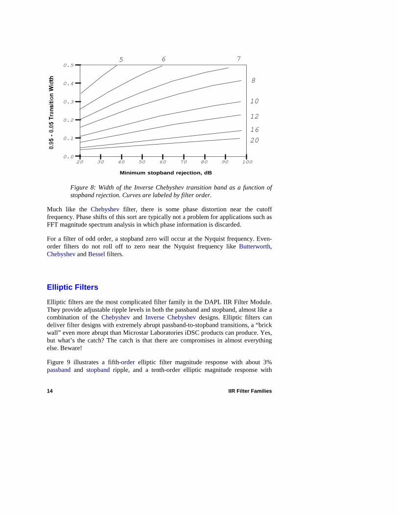
Figure 9 illustrates a fifth-order elliptic filter magnitude response with about 3% passband and stopband ripple, and a tenth-order elliptic magnitude response with


about 0.3% passband and stopband ripple. The sharp cutoff of the 10th order filter is quite dramatic. As with the Chebyshev and Inverse Chebyshev filter types, there is a tradeoff between ripple magnitudes and the width of the transition band.

0.0


0.1 0.2 0.3 0.4 0.5 0.7 0.8 0.9 1.00.6

0.0

0.1

0.2

0.3

0.5

0.6

0.7

0.8

0.9

1.0

0.4

Figure 9: Elliptic filter magnitude reponses of a 5th order filter with 3% ripple magnitude and a 10th order filter with 0.2% ripple magnitude.

But examining Figure 10 for the same 10th order filter shown in figure 9, it is clear that there are major phase disruptions.


-16.0

-14.0

-10.0

-8.0

-6.0

-4.0

-2.0

0.0

-12.0

0.0


0.1 0.2 0.3 0.4 0.5 0.7 0.8 0.9 1.00.6

Figure 10: Phase response of the 10th-order elliptic filter of Figure 9.

There are two gray bounding lines added to this figure. The sloping line shows the phase response of a filter with a phase lag proportional to frequency, or equivalently, a fixed time lag. That is how the elliptic filter behaves in roughly the first 2/3 of the passband. But approaching the cutoff frequency from that point, there is a major phase angle swing, covering approximately 2 pi radians. Frequencies near 90% of the cutoff frequency have a phase shift of about pi additional radians – these frequency components are completely inverted. This can be a serious problem. For example, if it is assumed that subtracting a filtered signal will cancel frequencies from the original data sequence, instead, these frequencies could be doubled rather than canceled!

In addition to the stopband ripple and passband ripple, filter design reference books typically introduce various other parameters to describe elliptic filters: the “transition parameter,” the “discrimination parameter,” the “ripple factor,” the “complete elliptic integral,” the “Jacobi sn function” and so on. All of these are interrelated in complicated ways. Most are unnecessary when using the elliptic filter family from the DAPL IIR Filter Module. Just specify a filter order, passband ripple and a stopband ripple, and all of the complicated mathematics will be done automatically.

One exception sometimes arises because elliptic filters are often specified in terms of a “transition width” property. The transition band for elliptic filters is defined as the interval from the passband edge, the frequency where the filter magnitude response first exceeds the maximum passband error, to the stopband edge, the first point that


meets minimum stopband rejection requirements. Elliptic filters have the property that the passband ends at frequency k1/2 Fc and the stopband begins at frequency 1/k1/2 Fc, where Fc is the desired cutoff frequency and k is a design parameter to be determined. Consequently, the transition band width is:

transition Fc k Fc k= −/

The parameter k characterizes the “steepness” of the transition, with the transition edge approaching vertical as the value of k approaches 1.0. In most cases, k is around 0.90 or so, and it sufficient to approximate

transition k Fc≈ −( . )10

For example, a transition parameter k of 0.90 yields a passband-to-stopband transition width of roughly 0.10 of passband width. Figure 11 illustrates the definition of the band edges and the correponding k parameter.

TransitionBandWidth

Figure 11: How an elliptic filter transition width is defined.

After establishing acceptable ripple levels for the passband and stopband, the reason for choosing a higher or lower filter order is to adjust the transition width as characterized by k. Here are two ways to determine what filter order is needed to meet a transition width requirements.

• FIRST ALTERNATIVE. Select a value for transition parameter k as described above. Compute the “discrimination parameter” d according to the formula:

dAp

As=−−

10 1010 10

0 1

0 1

.

...

for ripple expressed in decibels, or


( )( )

de

e

p

s

=−

−

−1

1 32768

2

132768

2

10

10

/

/

.

. for ripple expressed in integer counts.

where

ep = passband maximum ripple in unit counts

Ap = passband maximum ripple in decibels

es = stopband maximum ripple in unit counts

As = stopband minimum rejection (loss) in decibels

Locate the point on the graph in Figure 12 corresponding to the parameter pair (d,k). Identify the filter order corresponding to the first curve that lies above the identified point on the graph.

0.0

0.6

0.5

0.4

0.3

0.2

0.1

0.7

0.8

1.0

0.9

-6.0

Ripple discrimination parameter, d

-5.0 -4.0 -2.0 -1.0-3.0

643

578

1012

15

Figure 12: Elliptic filter transition width, as a function of intermediate discrimination parameter d. Curves are labeled by filter order.

• SECOND ALTERNATIVE. Use the following formulas to determine analytically what filter order is necessary to achieve a specified transition width.


1. Select a value for the transition parameter k, and compute “discrimination factor” d from the passband and stopband ripple as in the Second Alternative above.

2. Map the selected value of k into internal parameter q0 by the transformation

( )( )q

k

k0

2 14

2 14

12

1 1

1 1=

− −

+ −

( )

( )

3. Map q0 to internal parameter q by the series approximation q q q q q= + + +0 0

50

90132 15 150 . . .

4. Compute order parameter np from parameter q and d np d q= log ( ) / log ( )10

210

5. Pick filter order N as the first integer greater than or equal to np.

While elliptic filters are highly adjustable in passband and stopband and have excellent frequency sensitivity, they achieve this with compromises in the magnitude and phase response. So, use elliptic filters with care.

How Good Are The Filter Designs? 21

3. How Good Are The Filter Designs?

The goal of the digital filter approximation is to match the performance of analog filtering as closely as possible. In this section, we will examine the claim that the performance of the digital filters is virtually indistinguishable from the performance of their analog counterparts, comparing the subtle differences of corresponding analog and digital filters. The discussion will apply to all of the digital filter families.

1. Flatness properties of the analog filter designs are preserved exactly.

This is a provable mathematical property deriving from the prototype analog filter properties and the transformation technique that produces the digital filter designs.

2. Equi-ripple properties of the analog filter designs are preserved.

For the cases of analog filter families that have equi-ripple characteristics in passband or stopband, this is a provable mathematical property deriving from the prototype analog filter properties and the transformation technique that produces the digital filter designs.

3. Cutoff frequencies correspond exactly to the design specification.

This is not a natural property. It is enforced by the DAPL IIR Filter Module automated design algorithms.

The cutoff frequency is the frequency where the response magnitude is 0.70714 times the response magnitude in the passband. Or, equivalently the cutoff frequency is the frequency at which the filter response is reduced to half power. In the filter design literature, only the Butterworth filter is commonly defined in terms of cutoff frequency. However, all of the filters in the DAPL IIR Filter Module are specified by cutoff frequency. To do this, an additional frequency scaling operation is applied after the classical design steps, forcing the cutoff frequency to match the specification.

4. Critical frequencies are shifted.

Critical frequencies are features of the filter response such as minima, maxima or zero crossings. The transformation that maps frequencies from the continuous signal domain to the digital domain is

22 How Good Are The Filter Designs?

s zTzz= ≈ −+

1 12

11ln( )

This is a highly nonlinear mapping. Frequency 0 maps into z=1 exactly. The cutoff frequency is forced into exact alignment by applying a scaling factor to each s term in the analog model. All other frequencies are displaced.

• Passband ripple peaks are shifted very small amounts toward the cutoff frequency. These effects are usually negligibly small, and they are completely meaningless in flat portions of a passband.

• Stopband ripple peaks and zero crossings are shifted toward the cutoff frequency, to an increasing extent at higher frequencies.

The greatest differences occur in stopband ripple peaks and zero crossings near the Nyquist limit. For example, the following table lists stopband zero crossing frequencies of a ninth-order Inverse Chebyshev filter with cutoff at 25% of the Nyquist frequency and 1% ripple in the stopband.

Analog Model Digital Filter

Cutoff 0.2500 0.2500

Crossing 1 0.2991 0.2929

Crossing 2 0.3401 0.3267

Crossing 3 0.4583 0.4135

Crossing 4 0.8613 0.6109

Odd zero infinity 1.0000

Figure 13: Comparing zero-crossing locations of an Inverse Chebyshev analog filter prototype and the corresponding digital filter.

In most cases, features such as ripple peaks are undesirable artifacts that are intentionally made small enough that they are negligible, and therefore differences in their locations are of no consequence. However, a design that is depending on a zero crossing at a specific location must take the frequency shifts into account. If an analog filter design was selected to ensure a transmission zero at a specific stopband frequency, this property will not be preserved in the discrete filter. In most cases, small adjustments in the cutoff frequency can compensate for small shifts in the location of critical frequencies.


5. Passbands tend to be just slightly wider in the discrete filters.

Passband frequencies are also affected by frequency shifts, however, the effects are small because they are constrained by the alignment of frequency zero and the cutoff frequency. In most cases, the differences can be considered beneficial. The following table illustrates the slightly sustained passband levels for a ninth-order Butterworth filter.

frequency Analog Model Digital Filter

0.0938 0.9971 0.9974

0.1016 0.9883 0.9891

0.1172 0.8727 0.8756

0.1250 0.7071 0.7071

Figure 14: Slightly sustained passband in a ninth-order Butterworth filter with cutoff 1/8 of Nyquist frequency.

6. Transition bands tend to be just slightly narrower in discrete filters.

Frequency shifting effects tend to compress frequency features, producing filters with a very slightly narrower passband-to-stopband transition. In most cases, this can be considered beneficial. As an illustration, the following table shows the narrowing of the transition band for an eight-order Butterworth filter.

frequency Analog Model Digital Filter

transition start 0.1094 0.9576 0.9597

0.1133 0.9245 0.9273

transition end 0.1602 0.1062 0.0991

0.1641 0.0862 0.0792

24 How Good Are The Filter Designs?

Figure 15: Slight narrowing of transition band for a ninth-order Butterworth filter with cutoff 1/8 of Nyquist frequency.

7. Group delay (rate of phase change as a function of frequency) is slightly different in the digital and analog domains.

To illustrate this, the following plot shows the phase angle response of a ninth-order analog Butterworth filter and its digital approximation, with cutoff frequency 1/8 of the Nyquist limit.

-16.0

-14.0

-10.0

-8.0

-6.0

-4.0

-2.0

0.0

-12.0

0.00


0.05 0.10 0.15 0.20 0.25 0.35 0.40 0.45 0.500.30

Cutoff

Analog

Digital

Figure 16: Comparing analog prototype and digital realization for a 9th order Butterworth filter with cutoff at 1/8 of the Nyquist limit.

It is apparent in this plot that the phase differences are relatively small in the passband, with the greatest disturbances near the cutoff frequency. The phase angle begins to diverge in the stopband, and this continues at higher frequencies. The phase angle differences in the stopband are usually not a problem because the response magnitude is very low. Figure 17 plots the phase angle difference.


-0.30

-0.25

-0.15

-0.10

-0.05

0.00

0.05

0.10

-0.20

0.00


0.05 0.10 0.15 0.20 0.25 0.35 0.40 0.45 0.500.30

Figure 17: Phase angle difference between 9th-order analog Butterworth filter and its digital counterpart.

The phase angle differences are closely related to the frequency shifting that occurs when the analog filter is mapped into the digital domain.

Perhaps the worst hazard of the phase differences is that these compromise the phase linearity of the Bessel filter families. The effects are most apparent for filters with high cutoff frequencies.

Obtaining Detailed Design Information

If you have concerns that subtle differences between the discrete filter and analog filter characteristics are important to your application, you can obtain additional information about a filter design.

See the DAPview for Windows examples shipped with the product.

IIR Filter Parameters 27

4. IIR Filter Parameters

The procedures, notations and parameters described in engineering reference texts are different for each filter type. That is because each of the design methods was developed by a different mathematician, using different notations and mathematical tools. In the DAPL IIR Filter Module, all of the designs are specified by a simple and consistent set of parameters. Not only does this make the DAPL IIR Filter Module filters (without any exaggeration) the easiest package to use, it also greatly simplifies substitution of one filter type for another to facilitate field comparison in situations where the required filter properties are not clear a priori.

The parameters used to define the filter families for the DAPL IIR Filter Module are listed and discussed in detail below.

Filter Order

This number corresponds to the number of primitive first-order filter stages (states), each stage corresponding to one pole in the filter design. Most filter designs pair the filter stages to eliminate complex-valued intermediate terms, producing a filter with N/2 second-order stages plus an additional first-order stage when the filter order is odd. Pairing the filter stages does not change the filter order. Higher filter orders tend to deliver higher performance in terms of passband flatness, sharper transitions, and lower ripple, but the amount of computation grows in proportion to the filter order.

All of the filter families require a filter order parameter. Specify the filter order as an integer value. The order can range from 2 through 20 for all of the families except the elliptic, which will accept order 2 through 15.

Cutoff Frequency

Filtering frequencies are normalized so that the range 0.0 to 1.0 represents the frequency interval from 0.0 Hz to the Nyquist frequency (1/2 of sampling frequency). The cutoff can be specified using a fixed point or floating point notation. The maximum cutoff is 0.5 (1/4 of the sampling frequency).

If the cutoff is represented using a floating point notation, specify the cutoff frequency as a fraction of the Nyquist frequency. For example, if the sampling frequency is 10000 Hz, specifying a cutoff of 0.2 will produce a filter with cutoff frequency of 1000 Hz (2/10 of the Nyquist frequency of 5000 Hz).

28 IIR Filter Parameters

If the cutoff is represented using an integer notation, the integer range 0 through 32768 represents the frequency range from 0 to the Nyquist frequency. This can be useful in combination with FFT-based filtering or analysis.

For example, suppose that data is collected for an FFT analysis using blocks of 1024 samples of real-valued data. The FFT analysis will yield 512 samples covering from zero frequency through the Nyquist frequency. Then 32768/512 = 64, and filter cutoff frequencies that are multiples of 64 will correspond to the frequencies sampled in the FFT spectrum. To align a filter cutoff frequency at term 128 of the FFT, specify the filter cutoff 128*64 = 8192.

Passband Ripple

A passband ripple parameter is required for the Chebyshev and Elliptic filter families.

This parameter specifies the maximum amount that the passband gain can deviate from the nominal passband gain of 1.0. It can be specified using a floating point or a fixed point notation. Ripple magnitudes are limited to 2 dB or less. Figure 18 illustrates how passband ripple is defined.

(1-e)e

Maximum passband ripple = 32768*e

Minimum passbandgain =-20*log10(1-e)decibels

1.0

0.0

Figure 18: Definition of passband ripple parameters.

If a floating point notation is used to specify a passband ripple, it represents the signal gain at a point of minimum passband gain, (or equivalently maximum deviation from unity gain), expressed in decibels. Some useful special cases:

1. 0.1 dB, about 1.14% ripple, often used in high-quality analog audio filters,

IIR Filter Parameters 29

2. 0.01 dB, about 0.1% ripple, usually below a threshold of significance,

3. 0.00425 dB, about 16 counts peak error, one LSB for a 12-bit A-to-D converter,

4. 0.00106 dB, about 4 counts peak error, one LSB for a 14-bit A-to-D converter,

5. 0.0001325 dB, about 1 count peak error, the resolution of a 16-bit number.

If an integer notation is used to specify a passband ripple, the output level for any passband input frequency of maximum magnitude 32767 produces output peaks that differ from 32767 by at most by the specified amount.

For example, if the passband ripple parameter is set to 0.05 dB, the response of the filter can sag as low as 10(-0.05 / 20.0) = 0.99426 from its maximum of 1.0, for an error percentage of 0.574%. This same passband ripple can be specified by specifying a passband maximum error integer value 0.00574 x 32768 = 188 counts. With either notation, the maximum error in the passband given a sinusoidal wave with peak value 32767 is 188 counts.

Stopband Rejection

The Inverse Chebyshev and Elliptic filter families require a minimum stopband rejection (loss) parameter. This parameter specifies the maximum gain for any frequency in the stopband. It can be specified using a floating point or integer notation.

e

Minimumstopbandrejection =-20*log10(e)decibels

1.0

0.0

Maximumstopbandripple =32768 * e

Figure 19: Definition of stopband ripple parameters.

30 IIR Filter Parameters

If a stopband is specified using a floating point notation, it represents the minimum stopband rejection in decibels. Some useful special cases are:

• 30 dB, about 3.2% maximum response, or 1036 counts. • 40 dB, 1% maximum response, or 328 counts. • 60 dB, 0.1% maximum response, 33 counts. • 66 dB, 0.05% of maximum response, 16 counts, the output resolution of a 12-bit

D/A converter. • 96.3 dB, 1/65536, the resolution of a 16-bit number.

If the stopband ripple parameter is specified using an integer notation, it represents the maximum response level in integer counts when the input level is maximum for a frequency in the stopband.

For example, if the stopband rejection parameter is set to 50.0 dB, the response will never exceed the value 10(-50.0 / 20.0) = 0.003162 of the input signal level, for any frequency in the stopband. This corresponds to .003162 x 32768 = 103 counts output response for a stopband frequency driven at input maximum level.

Application Examples 31

5. Application Examples

This chapter provides application examples that illustrate the use of filters from this package.

Filter Families

In this first application, data is measured in a harsh environment using a sensor protected by an isolation amplifier. There is a ground voltage offset that drifts over time. Due to the high gains and high isolation impedances, there is a slowly drifting almost-constant voltage, with a magnitude comparable to the voltage level of the desired measurements. Frequencies below 1/2 Hz are considered to be due to the offset drift. Frequencies from 2 to 125 Hz are considered important to the application.

To get a good representation of the data at the upper end of the frequency range, a sampling frequency must be selected much higher than the highest frequency to be retained. The Nyquist limit would be 250 Hz, but as a practical matter, the analysis might require sampling at a rate higher than the theoretical absolute minimum. Assume that the sampling rate is set to 1000 Hz, or 4x oversampling. At this sampling rate, how large of a data block is necessary to distinguish 1/2 Hz from higher frequencies? Basically, there must be enough data to contain one complete cycle at 1/2 Hz. That is 2000 data points, a huge amount of data for a filter to process.

One approach to reducing the amount of computation is decimation. For detecting low frequencies, the higher frequency information can be removed by filtering. Fewer samples are needed to accurately represent the remaining low frequency signal, so the filtered data is decimated. The low frequency information is then much easier to filter in the decimated data stream. But then, to cancel the drift terms in the original data stream, the decimated stream must be replicated so that cancellation can be applied term by term.

This works, but it is somewhat cumbersome because of the filtering, decimation, re-filtering, replication and cancellation steps. Careful design of decimating and frequency discrimination filters is also required.

An alternative is to use the excellent low-frequency rejection properties of an IIR filter family for isolating the low frequencies. The filter must have a gain of exactly 1.0 at zero frequency, but a gradual magnitude deviation is acceptable approaching the

32 Application Examples

cutoff frequency. Small phase deviations are acceptable, but larger phase deviations would boost rather than cancel frequencies near the cutoff. A Butterworth filter characteristic has a flat response and relatively little phase disturbance, hence is considered the best filter family for this application. Examining Figure 2, if the filter cutoff is set to 1/2 Hz, a sixth-order filter has less than 5% response at 1 Hz and negligible response at 2 Hz.

The application configuration is as shown in Figure 21.

Anti-Alias for 1 KHz

BUTTERWORTH offset detect

HighSpeedSamples

- +

Application filtering

Figure 21 - Signal flow for offset drift cancellation application

Figure 21 also shows anti-aliasing filtering. This is necessary in all discrete sample systems when there is no guarantee that the external signal is free from non-random high frequency noise. Presume that the isolation amplifier and its circuits have a known natural cutoff frequency at 5 kHz. For data acquisition products such as the Microstar Laboratories iDSC series, the anti-alias filtering is built into the system. For this application example, assume a DAP series product that does not include onboard filters. Then the signal can be sampled at 5 kHz, and the DAPL command FIRLOWPASS used to implement anti-aliasing filtering with a factor of 5 decimation, to yield a clean sample sequence at a 1000 Hz sampling rate.

With a cutoff frequency at 1/2 Hz and a sampling frequency of 1000 Hz, the cutoff frequency for the Butterworth filter is 0.0005 of the sampling frequency, or 0.001 of the Nyquist limit. This number and the filter order are specified for the BUTTERWORTHBUTTERWORTHBUTTERWORTHBUTTERWORTH filtering command.

This application is now configured to run in the DAPL system using the following commands in the configuration script.

Application Examples 33

RESET CONSTANT cutoff FLOAT = 0.001 CONSTANT order WORD = 6 PIPES pclean WORD, plow WORD, pfiltered WORD IDEFINE sampling 1 SET IPIPE0 S0 TIME 200 END PDEF nodrift FIRLOWPASS(IPIPE0,5,pclean) BUTTERWORTH(pclean,order,cutoff,plow) pfiltered = pclean - plow // Application processing goes here END

IIR Filter Module Command Reference 35

6. IIR Filter Module Command Reference

This chapter provides detailed descriptions of command syntax and parameter list options.

Note: For a detailed discussion of magnitude and phase response in digital IIR filters, see Chapter 2. For information about the correspondence between the digital filters and their analog filter prototypes, see Chapter 3.

36 IIR Filter Module Command Reference

BESSEL

Define a task that applies an infinite impulse response lowpass filter of Bessel type to a data stream.

BESSEL (<in_pipe>, <order_N>, <cutoff>, <out_pipe>)

Parameters <in_pipe>

Input data pipe. WORD PIPE | FLOAT PIPE | DOUBLE PIPE

<order_N> The filter order. WORD CONSTANT

<cutoff> A value that specifies the cutoff frequency. WORD CONSTANT | FLOAT CONSTANT | DOUBLE CONSTANT

<out_pipe> Output data pipe. WORD PIPE | FLOAT PIPE | DOUBLE PIPE

Description BESSELBESSELBESSELBESSEL applies an infinite impulse response digital filter with response characteristics closely matching a lowpass analog Bessel filter. The filter accepts a data stream from <in_pipe> and delivers the filtered data stream to <out_pipe>. The data types of the <in_pipe> and <out_pipe> must be the same. The filter is characterized by the filter order <order_N> which corresponds to the number of filter stages in an analog filter design, and passband limit <cutoff> which is expressed as a fraction of the sampling Nyquist frequency. The filters are normalized to give a gain magnitude of 1.0 in the passband.

The cutoff frequency is specified using a positive word integer value or a floating point value. If the parameter is a floating point value, the value must be a positive fraction 0.0 < <cutoff> < 1.0. If the value is a word integer value, the range from 0 to 32768 represents the range from 0 to 100% of the Nyquist frequency. As a practical matter, very low values will exhibit undesirable numerical sensitivities and large response time constants, while very high values will not allow enough filter bandwidth for useful stop band attenuation.


The filter order <order_N> is restricted to the range 2 to 20. A first order filter is exactly equivalent to a lag filter. Higher order filters are subject to numerical sensitivity problems, hence are not supported. Higher-order filtering applications should consider a cascade of lower-order filters or FIRFILTERFIRFILTERFIRFILTERFIRFILTER as an alternative.

The Bessel filter is a causal (one-sided) filter. This allow it to respond with minimal delay, but at the costs of a loss of flatness in the passband and a very wide transition band. If it is not necessary to respond to the filtered signal with minimal latency, FIRFILTERFIRFILTERFIRFILTERFIRFILTER can provide superior passband flatness, excellent stopband attenuation, and much better transition width characteristics with lower computational overhead.


Examples BESSEL (FPIPE1, 12, 0.10, FPIPE2)

Apply a lowpass Bessel filter of order 12 to data from the input stream from floating point pipe FPIPE1, with filter cutoff frequency at 10% of the Nyquist frequency. Sent the results to floating point pipe FPIPE2.

See Also Bessel Filters, BUTTERWORTHBUTTERWORTHBUTTERWORTHBUTTERWORTH, CHEBYINVCHEBYINVCHEBYINVCHEBYINV, CHEBYSHEVCHEBYSHEVCHEBYSHEVCHEBYSHEV, ELLIPTICELLIPTICELLIPTICELLIPTIC, FIRFILTERFIRFILTERFIRFILTERFIRFILTER


BUTTERWORTH

Define a task that applies an infinite impulse response lowpass filter of Butterworth type to a data stream.

BUTTERWORTH (<in_pipe>, <order_N>, <cutoff>, <out_pipe>)






Description BUTTERWORTHBUTTERWORTHBUTTERWORTHBUTTERWORTH applies an infinite impulse response digital filter with response characteristics closely matching a lowpass analog Butterworth filter. The filter accepts a data stream from <in_pipe> and delivers the filtered data stream to <out_pipe>. The data types of the <in_pipe> and <out_pipe> must be the same. The filter is characterized by the filter order <order_N> which corresponds to the number of filter stages in an analog filter design, and passband limit <cutoff> which is expressed as a fraction of the sampling Nyquist frequency. The filters are normalized to give a gain magnitude of 1.0 in the passband.




The unity passband gain makes it is easy to use BUTTERWORTHBUTTERWORTHBUTTERWORTHBUTTERWORTH in combination with a DAPL expression to implement highpass filtering. Simply subtract the lowpass-filtered signal from the original signal to cancel out the low-frequency components.


Examples BUTTERWORTH (FPIPE1, 10, 0.10, FPIPE2)

Apply a lowpass Butterworth filter of order 10 to data from the input stream from floating point pipe FPIPE1, with filter cutoff frequency at 10% of the Nyquist frequency. Send the results to floating point pipe FPIPE2.

BUTTERWORTH (IPIPE1, 7, 328, PTEMP) P2 = IPIPE1-PTEMP

Use a Butterworth filter of order 7 and DAPL expression to remove low frequencies from the data stream in input channel pipe IPIPE1, placing the highpass filtered data into pipe P2. Use a lowpass filter cutoff frequency 328/32768, approximately 1% of the Nyquist frequency. Use word pipe PTEMP for the intermediate filter results.

See Also Butterworth filters, BESSELBESSELBESSELBESSEL, CHEBYINVCHEBYINVCHEBYINVCHEBYINV, CHEBYSHEVCHEBYSHEVCHEBYSHEVCHEBYSHEV, ELLIPTICELLIPTICELLIPTICELLIPTIC, FIRFILTERFIRFILTERFIRFILTERFIRFILTER


CHEBYINV

Define a task that applies an infinite impulse response lowpass filter of Inverse Chebyshev type to a data stream.

CHEBYINV (<in_pipe>, <order_N>, <cutoff>, <ripple>, <out_pipe>)





<ripple> A value that specifies the stopband ripple magnitude. WORD CONSTANT | FLOAT CONSTANT | DOUBLE CONSTANT


Description CHEBYINVCHEBYINVCHEBYINVCHEBYINV applies an infinite impulse response digital filter with response characteristics closely matching a lowpass analog Inverse Chebyshev filter. The filter accepts a data stream from <in_pipe> and delivers the filtered data stream to <out_pipe>. The data types of the <in_pipe> and <out_pipe> must be the same. The filter is characterized by the filter order <order_N> which corresponds to the number of filter stages in an analog filter design, a passband limit <cutoff> which is expressed as a fraction of the sampling Nyquist frequency, and a stopband ripple magnitude <ripple>. The filters are normalized to give a gain magnitude of 1.0 in the passband.

The cutoff frequency is specified using a positive word integer value or a floating point value. If the parameter is a floating point value, the value must be a positive


fraction 0.0 < <cutoff> < 1.0. If the value is a word integer value, the range from 0 to 32768 represents the range from 0 to 100% of the Nyquist frequency. As a practical matter, very low values will exhibit undesirable numerical sensitivities and large response time constants, while very high values will not allow enough filter bandwidth for useful stop band attenuation.

The ripple is specified using a positive word integer value or a floating point value. If the parameter is a floating point value, the value must be a positive fraction 0.0 < <ripple> << 1.0 and typically this number is very small. If the value is a word integer value, the range from 0 to 32768 represents the range from 0 to 100% of passband magnitude. For example, a <ripple> of 100 in the stopband corresponds to about 50 decibels minimum stopband loss. When stopband losses need to be bounded but not necessarily very large, the CHEBYINVCHEBYINVCHEBYINVCHEBYINV command provides a filter with good flatness in the passband, rapid stopband transition, and adjustable stopband loss with guaranteed minimum, but a less linear phase response than BUTTERWORTHBUTTERWORTHBUTTERWORTHBUTTERWORTH or BBBBESSELESSELESSELESSEL filters.

The filter order <order_N> is restricted to the range 2 to 20. A first order filter is exactly equivalent to a lag filter. Higher-order filtering applications should consider a cascade of lower-order filters or FIRFILTERFIRFILTERFIRFILTERFIRFILTER as an alternative.

The CHEBYINVCHEBYINVCHEBYINVCHEBYINV filter can be used in the manner of the BUTTERWORTHBUTTERWORTHBUTTERWORTHBUTTERWORTH filter, in combination with a DAPL expression, for highpass filtering. The flat passband of the CHEBYINVCHEBYINVCHEBYINVCHEBYINV will cause excellent cancellation of low frequencies, but the stopband ripples will affect the pass band response.


Examples CHEBYINV (P1, 6, 0.05, 64, P2)

Apply a lowpass Inverse Chebyshev filter of order 6 to data from the input stream from word pipe P1, with filter cutoff frequency at 1638/32768 of the Nyquist frequency, and allowing stopband deviations no greater than 64 counts (-54 dB minimum stopband loss). Send the results to word pipe P2.

See Also Inverse Chebyshev filters, BUTTERWORTHBUTTERWORTHBUTTERWORTHBUTTERWORTH, BESSELBESSELBESSELBESSEL, CHEBYCHEBYCHEBYCHEBYSHEVSHEVSHEVSHEV, ELLIPTICELLIPTICELLIPTICELLIPTIC, FIRFILTERFIRFILTERFIRFILTERFIRFILTER


CHEBYSHEV

Define a task that applies an infinite impulse response lowpass filter of Chebyshev type to a data stream.

CHEBYSHEV (<in_pipe>, <order_N>, <cutoff>, <ripple>, <out_pipe>)





<ripple> A value that specifies the passband ripple magnitude. WORD CONSTANT | FLOAT CONSTANT | DOUBLE CONSTANT


Description CHEBYSHEVCHEBYSHEVCHEBYSHEVCHEBYSHEV applies an infinite impulse response digital filter with response characteristics closely matching a lowpass analog Chebyshev filter. The filter accepts a data stream from <in_pipe> and delivers the filtered data stream to <out_pipe>. The data types of the <in_pipe> and <out_pipe> must be the same. The filter is characterized by the filter order <order_N> which corresponds to the number of filter stages in an analog filter design, a passband limit <cutoff> which is expressed as a fraction of the sampling Nyquist frequency, and a passband ripple magnitude <ripple>. The filters are normalized to give a peak gain magnitude of 1.0 in the passband.

The cutoff frequency is specified using a positive word integer value or a floating point value. If the parameter is a floating point value, the value must be a positive


fraction 0.0 < <cutoff> < 1.0. If the value is a word integer value, the range from 0 to 32768 represents the range from 0 to 100% of the Nyquist frequency. As a practical matter, very low values will exhibit undesirable numerical sensitivities and large response time constants, while very high values will not allow enough filter bandwidth for useful stop band attenuation.

The ripple is specified using a positive word integer value or a floating point value. If the parameter is a floating point value, the value must be a positive fraction 0.0 < <ripple> << 1.0 and typically this number is very small. If the value is a word integer value, the range from 0 to 32768 represents the range from 0 to 100% of passband magnitude. For example, a 0.1 dB ripple magnitude corresponds to about 1.2%, which can be represented as a ripple parameter of 0.012 or as 393. When small deviations in passband phase and magnitude are acceptable, the CHEBYSHEVCHEBYSHEVCHEBYSHEVCHEBYSHEV command provides a filter with better cutoff and transition band characteristics compared to the BUTTERWORTHBUTTERWORTHBUTTERWORTHBUTTERWORTH filter.


The filter order <order_N> is restricted to the range 2 to 20. A first order filter is exactly equivalent to a lag filter. Higher-order filtering applications should consider a cascade of lower-order filters or FIRFILTER as an alternative.

The CHEBYSHEVCHEBYSHEVCHEBYSHEVCHEBYSHEV filter can be used in the same manner of the BUTTERWORTHBUTTERWORTHBUTTERWORTHBUTTERWORTH filter, in combination with a DAPL expression for highpass filtering. Just keep in mind that the passband ripples of the CHEBYSHEVCHEBYSHEVCHEBYSHEVCHEBYSHEV filter will lead to incomplete cancellation of low frequencies, resulting in response peaks that limit stopband loss in highpass operation.


Examples CHEBYSHEV (FPIPE1, 5, 1638, 0.025 FPIPE2)

Apply a lowpass Chebyshev filter of order 5 to data from the input stream from floating point pipe FPIPE1, with ripple in the filter passband no larger than 2.5%, and with filter cutoff frequency at 1638/32768 of the Nyquist frequency. Send the results to floating point pipe FPIPE2.

See Also Chebyshev filter, BUTTERWORTHBUTTERWORTHBUTTERWORTHBUTTERWORTH, BESSELBESSELBESSELBESSEL, CHEBYINVCHEBYINVCHEBYINVCHEBYINV, ELLIPTICELLIPTICELLIPTICELLIPTIC, FIRFILTERFIRFILTERFIRFILTERFIRFILTER


ELLIPTIC

Define a task that applies an infinite impulse response lowpass filter of Elliptic type to a data stream.

ELLIPTIC (<in_pipe>, <order_N>, <cutoff>, <P_ripple>, <S_ripple>, <out_pipe>)





<P_ripple> A value that specifies the passband ripple magnitude. WORD CONSTANT | FLOAT CONSTANT | DOUBLE CONSTANT

<S_ripple> A value that specifies the stopband ripple magnitude. WORD CONSTANT | FLOAT CONSTANT | DOUBLE CONSTANT


Description ELLIPTIC applies an infinite impulse response digital filter with response characteristics closely matching a lowpass analog elliptic filter. The filter accepts a data stream from <in_pipe> and delivers the filtered data stream to <out_pipe>. The data types of the <in_pipe> and <out_pipe> must be the same. The filter is characterized by the filter order <order_N> which corresponds to the number of filter stages in an analog filter design, a passband limit <cutoff> which is expressed as a fraction of the sampling Nyquist frequency, a maximum passband ripple magnitude<ripple> and a maximum stopband ripple magnitude


<ripple>. The filters are normalized to give a peak gain magnitude of 1.0 in the passband.



Ripple parameters are specified using either a positive word integer value or a floating point value. If the parameter is a floating point value, the value must be a positive fraction 0.0 < <ripple> << 1.0 and typically this number is very small. If the value is a word integer value, the range from 0 to 32768 represents the range from 0 to 100% of passband magnitude.

An elliptic filter is typically used in situations where a very rapid “brick wall” response characteristic is needed, but rather large phase shifts near the cutoff frequency are not a problem. Ordinarily, stopband and passband ripple limits are specified, and then a filter order is selected to give a sufficiently narrow transition width. Elliptic filters are best applied in special situations where a highly selective cutoff characteristic is necessary, and speed is more important than accurate passband gains or high stopband rejection.


Examples ELLIPTIC (P1, 5, 1638, 0.01, 0.002, P2)

Apply a lowpass Elliptic filter of order 5 to data from the input stream from word pipe P1, with filter cutoff frequency at 1638/32768 of the Nyquist frequency, and allowing passband ripple of no more than 1.0% and stopband ripples of no more than 0.2% (-54 dB). Send the results to word pipe P2.

See Also Elliptic filters, BUTTERWORTHBUTTERWORTHBUTTERWORTHBUTTERWORTH, BESSELBESSELBESSELBESSEL, CHEBYINVCHEBYINVCHEBYINVCHEBYINV, CHEBYSHEVCHEBYSHEVCHEBYSHEVCHEBYSHEV, FIRFILTERFIRFILTERFIRFILTERFIRFILTER


FIRFILTER

See the DAPL 2000 Reference Manual for a description of the FIRFILTER command.

Index 53

Index Application Examples ............................................................................................................... 31 Bessel ................................................................................................................ 12, 14, 25, 36, 38 BESSEL...................................................................................................... 36, 41, 43, 44, 48, 51 Bessel Filters............................................................................................................................... 8 Butterworth ........................................................... 7, 8, 10, 11, 12, 13, 14, 21, 23, 24, 32, 39, 41 BUTTERWORTH............................................................... 32, 38, 39, 40, 43, 44, 46, 47, 48, 51 Butterworth Filters ...................................................................................................................... 7 CHEBYINV................................................................................................ 38, 41, 42, 43, 48, 51 Chebyshev............................................................................................. 12, 13, 14, 15, 28, 45, 48 CHEBYSHEV....................................................................................... 38, 41, 44, 45, 46, 47, 51 Chebyshev Filters...................................................................................................................... 10 cutoff........................................................................................................... 15, 36, 39, 42, 45, 49 cutoff frequency .............................................................................. 10, 11, 12, 36, 39, 42, 45, 50 Cutoff frequency ....................................................................................................................... 27 cutoff region................................................................................................................................ 8 Digital and Analog Filtering ....................................................................................................... 1 Digital Filters

Finite or Infinite Response ..................................................................................................... 3 Elliptic................................................................................................................................. 28, 29 ELLIPTIC ......................................................................................................... 38, 41, 44, 48, 49 elliptic filter............................................................................................................................... 49 Elliptic filter .............................................................................................................................. 51 Elliptic Filters ........................................................................................................................... 14 families........................................................................................................................................ 8 filter families ............................................................................................. 2, 7, 21, 25, 27, 28, 29 Filter Families ........................................................................................................................... 31 filter family................................................................................................................................ 31 filter order ............................................... 7, 13, 16, 17, 18, 32, 36, 37, 39, 40, 42, 45, 47, 49, 50 Filter order ................................................................................................................................ 27 filter orders................................................................................................................................ 11 Filters

Analog and Digital.................................................................................................................. 2 FIRFILTER..................................................................... 3, 37, 38, 40, 41, 43, 44, 48, 50, 51, 52 How Good Are The Filter Designs?.......................................................................................... 21 IIR Filter Families....................................................................................................................... 7 IIR Filter Module Command Reference.................................................................................... 35 IIR Filter Parameters ................................................................................................................. 27 Inverse Chebyshev ...................................................................................... 14, 15, 22, 29, 42, 44 Inverse Chebyshev Filters ......................................................................................................... 12 Obtaining Detailed Design Information .................................................................................... 25 order.......................................................................................................................... 8, 10, 14, 15 passband.................................................................................................................................... 14

54 Index

passband ripple ................................................................................................. 10, 11, 16, 45, 49 Passband Ripple........................................................................................................................ 28 ripple............................................................................................................................. 12, 43, 46 stopband.................................................................................................................................... 14 Stopband Rejection................................................................................................................... 29 stopband ripple ............................................................................................................. 16, 42, 49 Why Filter? ................................................................................................................................. 1

Documents

DAPL IIR Filter Module Manual - Microstar Laboratories