DBN Structure Design Algorithm for Different Datasets Based

entropy

Article

DBN Structure Design Algorithm for DifferentDatasets Based on Information Entropy andReconstruction Error

Jianjun Jiang *, Jing Zhang, Lijia Zhang, Xiaomin Ran, Jun Jiang and Yifan Wu

National Digital Switching System Engineering and Technological Research Center (NDSC), Zhengzhou 450000,Henan, China; [email protected] (J.Z.); [email protected] (L.Z.); [email protected] (X.R.);[email protected] (J.J.); [email protected] (Y.W.)* Correspondence: [email protected]; Tel.: +86-150-3823-2583

Received: 23 October 2018; Accepted: 2 December 2018; Published: 4 December 2018��

Abstract: Deep belief networks (DBNs) of deep learning technology have been successfully used inmany fields. However, the structure of a DBN is difficult to design for different datasets. Hence, a DBNstructure design algorithm based on information entropy and reconstruction error is proposed. Unlikeprevious algorithms, we innovatively combine network depth and node number and optimizes themsimultaneously. First, the mathematical model of the structural design problem is established, andthe boundary constraint for node number based on information entropy is derived by introducing theidea of information compression. Moreover, the optimization objective of the network performancebased on reconstruction error is proposed by deriving the fact that network energy is proportionalto reconstruction error. Finally, the improved simulated annealing (ISA) algorithm is used to adjustthe DBN network layers and nodes simultaneously. Experiments were carried out on three publicdatasets (MNIST, Cifar-10 and Cifar-100). The results show that the proposed algorithm can designits proper structure to different datasets, yielding a trained DBN which has the lowest reconstructionerror and prediction error rate. The proposed algorithm is shown to have the best performancecompared with other algorithms and can be used to assist the setting of DBN structural parametersfor different datasets.

Keywords: deep learning; DBN; artificial intelligence; structure design; information entropy;reconstruction error; improved simulated annealing algorithm

1. Introduction

A deep belief network (DBN) is a kind of deep artificial neural network (ANN) [1]. An ANN,which originated from Rosenblatt’s perceptron model, is an information processing network composedof simple nodes that has nonlinear fitting ability [2]. In 2006 and later, Hinton proposed the DBN [3] andCD-K [4] algorithms, which has enabled ANNs to develop from a shallow to deep structure, achievingsignificant performance improvements. As a typical type of deep network [5], DBNs are widely usedin image processing [6–10], speech recognition [11–13] and nonlinear function prediction [14], yieldingexcellent performance. However, DBNs still have many problems worth studying, such as the networkstructure design [15–19], selection and improvement of training algorithms [20,21], introduction ofautomatic encoders, and implementation of GPU parallel acceleration [22,23]. In particular, the designof DBN network structures is of high research significance.

The performance of a DBN is closely related to its structure. A simple structure can improve theconvergence speed, but it may lead to problems such as low training precision and large prediction error.A complex structure can improve the training precision, but it can easily lead to non-convergence or

Entropy 2018, 20, 927; doi:10.3390/e20120927 www.mdpi.com/journal/entropy

http://www.mdpi.com/journal/entropy

http://www.mdpi.com

http://www.mdpi.com/1099-4300/20/12/927?type=check_update&version=1

http://dx.doi.org/10.3390/e20120927

http://www.mdpi.com/journal/entropy

Entropy 2018, 20, 927 2 of 18

over-fitting. In engineering practice, experience or trial-and-error method are often used in traditionalANN structure design [2,24]. However, because a DBN is deep, with numerous nodes and a complexstructure, it is difficult to find the optimal structure using these methods, and the network performancecan-not be guaranteed. In addition, these approaches do not result in a network that can self-adapt,which is needed to redesign it for different data sets.

Given the above problems, some researchers have studied DBN structure design. In terms ofnetwork depth, Pan et al. proposed using the correlation inference of network energy, networkperformance, and depth [15]. Gao et al. determined the number of DBN layers using the correlation ofhidden layers [16]. But them only analyzed the depth with ignoring the relationship between the numberof nodes and the number of layers. Stathakis designed a fitness function to solve the optimal networkstructure by combining the coding and optimization process of genetic algorithm [18]. However, it isnot suitable for the process of unsupervised training. In terms of the number of hidden-layer neurons,researchers have proposed various strategies such as using the data dimensionality as the number ofnodes [21], using more nodes than the data dimensionality [20], the minimizing the error to determinethe node number, and using a symmetric hidden layer structure [21].

Previous studies have preliminarily discussed the design method for a DBN structure, but theyhave only discussed a single aspect of structure, either network depth or the number of nodes. Or, theydid not fully consider the unsupervised training process of the DBN network. In fact, the performanceof a network is determined by both aspects. The two parameters are coupled and hence influenceeach other. The optimal value of the depth is related to the node selection strategy, and the optimalvalue of the number of nodes is related to the depth optimization strategy. If we combine the depthdecision and the node optimization processes while ignoring the organic correlation between them,it is difficult to obtain a good network structure. Therefore, to improve the performance of DBN bychanging its structure, we need a DBN structure design algorithm that simultaneously and organicallycombines network depth and node number.

Hence, this paper proposes a DBN structural design algorithm based on information entropyand reconstruction error. The algorithm innovatively combines the network depth and number ofnodes into a unified mathematical model, introduces information entropy and reconstruction error,and uses the ISA algorithm to solve the optimization problem. First, using information compressionand the distribution characteristics of the sample, a bound on the number of hidden layer neuronsbased on information entropy is derived. In addition, the positive correlation between reconstructionerror and network energy is proved, and a model optimization that minimizes the reconstruction erroris constructed. Then, this paper employs the ISA algorithm to solve for the network depth and nodenumber while training the network. The experimental results show that this algorithm can generatea network structure that is adapted to different datasets. Moreover, the constructed DBN has lowerreconstruction and root-mean-square errors in training process as well as a low prediction error rate intest process.

2. Structure Optimization Model of a DBN

The DBN structure is determined by the number of layers and the number of nodes (or neurons)contained in each layer. Therefore, to adjust the structure, it is essential to automatically solve forthe optimal number of layers and nodes for each data set. From the perspective of mathematicalmodeling, this problem can be expressed as an optimization in the solution space formed by all feasibleDBN structures. Therefore, for the general optimization model, the problem can be mathematicallyexpressed in the framework of an objective function and constraint conditions as follows:

min f (x) x ∈ Xs.t. gi(x) = 0 i = 1, 2, . . .

hj(x) ≤ 0 j = 1, 2, . . .(1)

Entropy 2018, 20, 927 3 of 18

where, f (x) denotes the target function and gi(x) and hj(x) denote equality constraints and inequalityconstraints, respectively. For the problem of DBN structure design, this paper derives and provestwo conclusions:

Conclusion 1. The range of the number of hidden-layer neurons is based on the information entropy.

Conclusion 2. The network performance is based on reconstruction error.

Hence, the DBN structure optimization model is constructed as follows:

min R(C) C ∈ Cs.t. Nmin(k) ≤ Nhid(k) ≤ Nmax(k), ∀k ∈ 1 . . . n

D ≤ Dmax

(2)

Here, C represents the DBN structure and C represents the solution space formed by all feasibleDBN structures, R(C) indicates the DBN reconstruction error in structure C, k represents the index ofthe restricted Boltzmann machine (RBM) in the DBN from 1 to n, Nhid(k) denotes the number of hiddenlayer neurons in the k-th RBM, and Nmin(k) and Nmax(k) represent the minimum and maximum valuesof the number of neurons in the hidden layer in the k-th RBM, respectively. Finally, D represents thedepth of the DBN network and Dmax represents the maximum depth of the network that meets therequirements. The physical meaning of the mathematical model is to find the network structure thatminimizes the reconstruction error on the basis of satisfying the boundary for the number of neuronsand the upper bound of the depth of network. Sections 2.1 and 2.2 of this paper detail the derivationof Conclusions 1 and 2, respectively.

2.1. Lower Bound of the Number of Hidden Neurons

The DBN consists of multiple layers of neurons, where each two adjacent layers of neurons makeup one RBM, as shown in Figure 1. Each RBM has a bipartite graph structure. According to the inputand output, the neurons are divided into a visible layer and hidden layer. Each neuron only performslayer interconnection and does not perform intra-layer interconnection. Each layer of neurons canbe used as both a hidden layer for the current RBM and a visible layer for the next RBM. Therefore,a DBN can be regarded as a deep network in which multiple RBMs are stacked.

Entropy 2018, 20, x FOR PEER REVIEW 3 of 18

where, ( )f x denotes the target function and ( )ig x and ( )jh x denote equality constraints and inequality constraints, respectively. For the problem of DBN structure design, this paper derives and proves two conclusions:

Conclusion 1: The range of the number of hidden-layer neurons is based on the information entropy.

Conclusion 2: The network performance is based on reconstruction error.

Hence, the DBN structure optimization model is constructed as follows:

( ) ( )min hid max

max

min ( ) s.t. ( ) , 1...

R C CN k N k N k k nD D

∈≤ ≤ ∀ ∈

≤

. (2)

Here, C represents the DBN structure and represents the solution space formed by all feasible DBN structures, ( )R C indicates the DBN reconstruction error in structure C, k represents the index of the restricted Boltzmann machine (RBM) in the DBN from 1 to n ,

hid ( )N k denotes the number of hidden layer neurons in the k-th RBM, and ( )minN k and ( )maxN k represent the minimum and maximum values of the number of neurons in the hidden layer in the k-th RBM, respectively. Finally, D represents the depth of the DBN network and maxD represents the maximum depth of the network that meets the requirements. The physical meaning of the mathematical model is to find the network structure that minimizes the reconstruction error on the basis of satisfying the boundary for the number of neurons and the upper bound of the depth of network. Sections 2.1 and 2.2 of this paper detail the derivation of Conclusions 1 and 2, respectively.

2.1. Lower Bound of the Number of Hidden Neurons

The DBN consists of multiple layers of neurons, where each two adjacent layers of neurons make up one RBM, as shown in Figure 1. Each RBM has a bipartite graph structure. According to the input and output, the neurons are divided into a visible layer and hidden layer. Each neuron only performs layer interconnection and does not perform intra-layer interconnection. Each layer of neurons can be used as both a hidden layer for the current RBM and a visible layer for the next RBM. Therefore, a DBN can be regarded as a deep network in which multiple RBMs are stacked.

Train data

...

...

...

……

Output

Labels

RBM1

BP

W0

W1

WD

RBM0

V0

H0

V1

H1

V2

Figure 1. RBM structure in a DBN.

The process of transferring data from the visible layer to the hidden layer in an RBM is a dimensionality-reducing feature extraction process [25]. Its purpose is to represent high-dimensional input data using a low-dimensional output vector through network mapping. This feature extraction process, from the viewpoint of information theory, is an information compression process:

Figure 1. RBM structure in a DBN.

The process of transferring data from the visible layer to the hidden layer in an RBM is adimensionality-reducing feature extraction process [25]. Its purpose is to represent high-dimensionalinput data using a low-dimensional output vector through network mapping. This feature extractionprocess, from the viewpoint of information theory, is an information compression process: eliminating

Entropy 2018, 20, 927 4 of 18

the redundant information in the input and using a smaller number of coded bits to achieve the storageof information.

Based on the idea of information compression, when determining the number of hidden-layernodes, it must be ensured that the maximum amount of information that the hidden layer outputvector can store is greater than or equal to the amount of information carried by the input data ofthe visible layer, so that information will be transferred losslessly. Otherwise, information will beinevitably lost, and this will ultimately reduce the overall network performance. Therefore, this paperemploys the information entropy as the criterion for determining the number of hidden layer nodes.

Information entropy, proposed by Shannon, is a measure of information quantity. In physicalsense, it refers to the uncertainty of the received signal. The formula for calculating the informationentropy of a single character is:

H =J

∑i=1

p(i) log1

p(i)(3)

where, H is information entropy, J is the number of characters, and p(i) indicates the probability of

receiving character i, whereJ

∑i=1

p(i) = 1.

Equation (3) shows that a larger signal uncertainty leads to a larger amount of information.Moreover, when all the probability values are equal, the amount of information of the characteris maximized.

Let the number of visual layer nodes be Nviso, the probability that the state of the i-th node in alayer equals zero be denoted by Pi(0), and the probability that the state is equal to one be denoted byPi(1). Then, the information entropy Hviso of the RBM visual layer is calculated by:

Hviso =Nviso

∑i=1

[pi(0) log

1pi(0)

+ pi(1) log1

pi(1)

](4)

Further, let the number of hidden layer nodes be Nhid, the probability that the state of the i-thnode in the layer equals zero be denoted by p′i(0), the probability that the state is equal to one bedenoted by p′i(1), and the hidden layer’s overall information volume be denoted by Hhid. Because thestate of the hidden layer neurons of DBN can only be zero or one, so the maximum value Hmax

hid of Hhidis reached at p′i(0) = p′i(1) =

12 :

Hmaxhid =

Nhid∑i−p′i(0) log2

(p′i(0)

)− p′i(1) log2

(p′i(1)

)=

Nhid∑i

12 log2

(12

)+ 1

2 log2

(12

)= Nhid

(5)

Because the maximum amount of information that the hidden layer output vector can storeis greater than or equal to the amount of information carried by the input data of the visible layer,we obtain:

Hmaxhid ≥ Hviso. (6)

From Equations (5) and (6), we can get:

Nhid ≥ Hviso. (7)

Obviously, Equation (7) gives the lower bound of the number of nodes in the hidden layer as follows:

Nmin(k) = Hviso(k). (8)

To obtain a more reasonable network, the maximum number of neurons in each hidden layer isdefined according to [4,21], which use the same number of neurons for the hidden layers. This paper

Entropy 2018, 20, 927 5 of 18

sets the number of nodes for each hidden layer to be no greater than the number of nodes in the inputlayer. Let Ni be the number of nodes in the current layer, and N0 be the number of nodes in the inputlayer. The value range of the number of nodes is as follows:

Nhid ≤ N0 (9)

From Equation (9), the upper bound of the hidden layer nodes can be obtained as:

Nmax(k) = N0 (10)

From the above analysis, we hence obtain Conclusion 1, and the range of the number of hiddenlayer nodes based on information entropy is Hviso ≤ Nhid ≤ N0.

2.2. DBN Performance Measurement Based on Reconstruction Error

To optimize the network structure, we need to introduce an index that can reflect the performanceof DBN. According to [20], we have the following lemma:

Lemma 1. Network energy is an important index for judging the performance of feedback network, and itsnumerical value is inversely proportional to the network performance.

Network energy is calculated as:

L =1T

T

∑t=1

[Nviso

∑i

Nhid

∑j

Wijvi(t)hj(t) +Nviso

∑i

aivi(t) +Nhid

∑j

bjhj(t)

](11)

Here, L represents the network energy, T represents the total number of training samples,W represents the weight matrix, vi(t) represents the value of the i-th visible-layer neurons, hj(t)represents the value of the j-th hidden-layer neurons, ai represents the bias of the i-th visible-layerneurons, and bj represents the bias of the j-th hidden-layer neurons. A lower network energy indicatesa better network performance.

Therefore, in theory, network energy can be used as an optimization objective. However,the computational complexity of network energy is high, which may lead to impractically longcomputation times and memory overflow. Hence, in this paper, based on [15], the relationship betweenreconstruction error and network energy is derived, and a network performance metric based onreconstruction error is proposed.

The reconstruction error refers to the difference between the samples obtained by Gibbs samplingand the original data. The calculation of reconstruction error R is:

R =

T∑

t=1v(t)− v0(t)

T(12)

Here, v0(t) denotes the original data and v(t) denotes the value obtained by Gibbs sampling.Because the input of samples is stationary processes, when T is large enough:

T∑

t=1v(t)

T= E(v) = ∑

kpv(k)k (13)

T∑

t=1vo(t)

T= E(vo) = ∑

kpv0(k)k (14)

Entropy 2018, 20, 927 6 of 18

Here, E(•) denotes the expectation, pv(k) denotes the probability that reconstruction value vequals k (this is also called posteriori probability), and pv0(k) as the probability that reconstructionvalue v0 equals k (this is also called priori probability). Combining Equations (12)–(14), we get:

R = ∑k

k[pv(k)− pv0(k)] (15)

In RBMs, we use v0 to denote the original data of the visible layer, v to denote the value afterreconstruction, and h to denote the value of hidden layer. For convenience of discussion, the probabilitydistribution of v is p(v), the probability distribution of v0 is p(v0), and the probability distributionof h is p(h). According to conditional probability and total probability formula, p(v) is calculatedas follows:

p(v) = ∑h

p(v|h)p(h)

= ∑h

p(v|h)∑v0

p(h|v0)p(v0)

= ∑h

∑v0

p(v,h)p(h)

p(h,v0)p(v0)

p(v0)

= ∑h

∑v0

p(v, h) p(v0,h)p(h) = ∑

h∑v0

p(v, h)p(v0|h)

(16)

Because p(v0) belongs to priori probability, p(v0|h) = p(v0). Equation (15) can be rewrittenas follows:

R = ∑k

k

[∑h

∑v0

pv,h(k, h)pv0(k)− pv0(k)

](17)

Because pv0(k) is only related to the training data and has nothing to do with the network,the following statement can be obtained from Equation (17):

R ∝ pv,h(k, h) (18)

Combining Equation (11) and the energy-based model of RBM, pv,h(k, h) has the followingrelationship with network energy L:

pv,h(k, h) =eL

Z(19)

Here Z is a normalized denominator that is determined only by the network parameters.Therefore, according to Equation (19), we obtain:

pv,h(k, h) ∝ L (20)

Moreover, according to Equations (18) and (19), we have:

R ∝ pv,h(k, h) ∝ L (21)

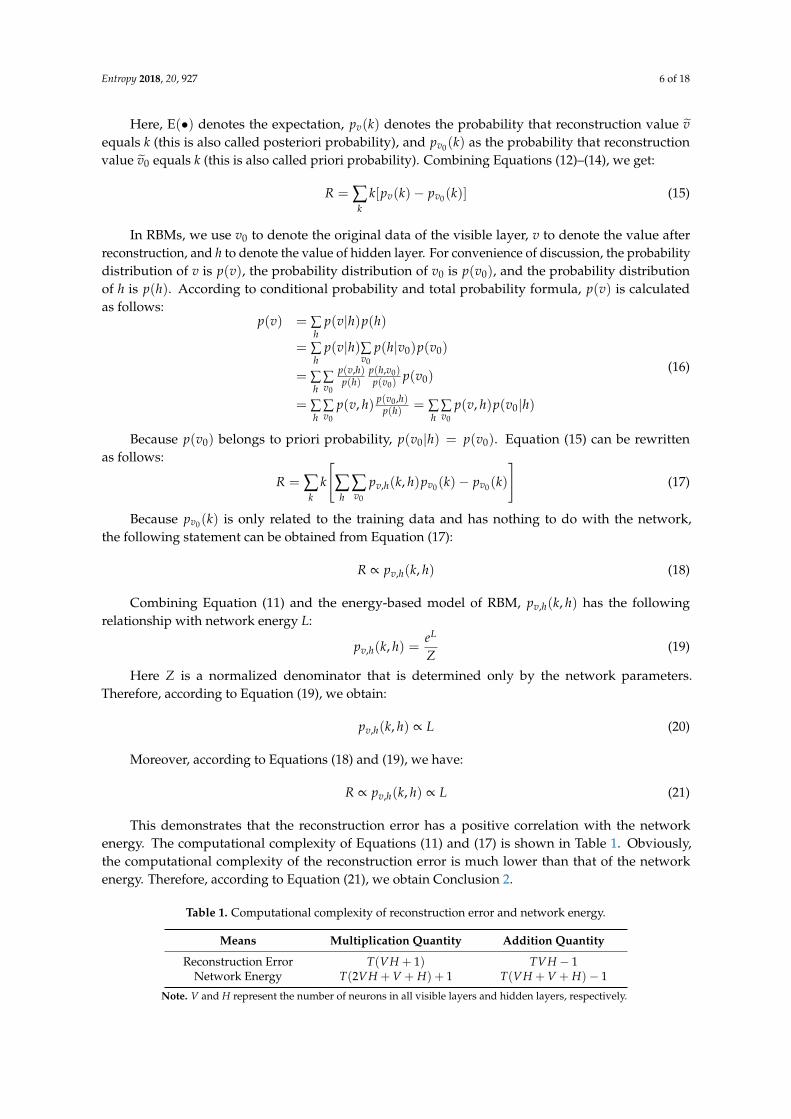
This demonstrates that the reconstruction error has a positive correlation with the networkenergy. The computational complexity of Equations (11) and (17) is shown in Table 1. Obviously,the computational complexity of the reconstruction error is much lower than that of the networkenergy. Therefore, according to Equation (21), we obtain Conclusion 2.

Table 1. Computational complexity of reconstruction error and network energy.

Means Multiplication Quantity Addition Quantity

Reconstruction Error T(VH + 1) TVH − 1Network Energy T(2VH + V + H) + 1 T(VH + V + H)− 1

Note. V and H represent the number of neurons in all visible layers and hidden layers, respectively.

Entropy 2018, 20, 927 7 of 18

3. Structure Design Using ISA

For the optimization model established in the Section 2, a suitable algorithm can be adopted.The simulated annealing (SA) algorithm has many advantages [26], such as a simple structure, flexibility,and high efficiency. At the same time, the simulated annealing algorithm has been theoretically provedto be a global optimization algorithm [27]. Moreover, the network performance oscillation caused bythe DBN structure optimization process is similar to the “heating” and “cooling” procedure of theSA algorithm, so this algorithm is easily incorporated into DBN structure design. Hence, this sectionexplains how we employ the SA algorithm to optimize the mathematical model described in Section 2.

The SA algorithm is a general probabilistic search algorithm that simulates the annealing processof solid matter in physics. It has a fast search speed and excellent globally optimal search ability.The core concept of SA is to construct a state transition probability matrix and update the currentsolution according to the matrix. The probability of a transition from state 1 to state 2 p(1→ 2) is:

p(1→ 2) =

{1, Y2 < Y1

exp(−Y2−Y1

τ

), Y2 > Y1

(22)

Here, τ is the “temperature”, which is the artificially set control algorithm iteration rate,Y1 and Y2 are the internal energies of state 1 and 2, respectively, and the state energy Y is theoptimization objective.

In addition, let τ be gradually reduced in each iteration according to:

τk+1 = ατk (23)

Here, α denotes the descending factor, α < 1, to ensure τ decreases. Obviously, combiningEquations (22) and (23), as the temperature τ gradually decreases, the system state will graduallyconverge to a low energy state and eventually reach the lowest point of the internal energy, that is,the minimum value of the optimization target.

The traditional SA algorithm has some disadvantages, such as sensitive parameters,poor convergence performance, and a tendency to fall into local optima. Therefore, according to [27],the global search performance of SA can be improved by adding memory and return search functions.The improved algorithm is called the ISA algorithm.

In order to study the DBN structure design based on ISA algorithm, two lemmas are introduced.

Lemma 2. the fitting accuracy of the network increases as the number of network layers increases, when thenumber of training samples is sufficient [15].

Lemma 3. increasing network depth can improve network performance more effectively than increasing networkwidth [28].

Combining Conclusions 1 and 2, we obtain the following three Rules.

1. The internal energy of the solution in the ISA algorithm is equal to the reconstruction error of theRBM at the highest level of the DBN.

From Conclusion 2 and Lemma 2, we obtain that the reconstruction error of the topmost RBMreflects the upper bound of the performance of the whole network structure, which is the optimizationgoal of the model. Hence, we obtain a second rule.

2. The undetermined new solution of the number of nodes in the layer is randomly generated,and the state update follows Equation (22).

The number of nodes Ni in the layer is randomly generated from the average probabilitydistribution, where the probability of each value is P = 1

M and M is the total number of possible

Entropy 2018, 20, 927 8 of 18

values. Based on Conclusion 1 and Equation (8), the number of neuron nodes in the current layer Niand the number of nodes in the next layer Ni−1 have the following relationship:

N0 ≥ Ni ≥ log2(Ni−1) (24)

Hence, we obtain the following equation:

M = N0 − ceil(log2(Ni−1)) (25)

According to the Metropolis rules, if N′i denotes the undetermined new solution, then theprobability of accepting state update Ni → N′i is calculated according to Equation (22), where thereconstruction error Y2 under N′i is substituted into R′i and the reconstruction error Y1 under Ni isreplaced by Ri. We finally have a third rule.

3. The number of layers increases monotonically from simple to complex.

According to Lemma 3, the effect of the upper layer nodes on performance is much higher thanthat of the lower layer nodes, so the complexity of the network structure is gradually improved by alayer-by-layer approach. The number of nodes in the bottom layer is optimized first then fixed. Then, ineach subsequent iteration, only the number of nodes in the next layer of the network is adjusted.

The pseudocode of the resulting DBN structure design algorithm is shown in Algorithm 1.

Algorithm 1: DBN Structure Design Algorithm via ISA

1: Initialization: set initial temperature τ0, minimum temperature τmin, intra-layer iterationlimit Dmax, network overall iteration limit Gmax, objective function threshold Rend, initialnetwork depth D = 2 (input layer and output layer), and memory matrix I.

2: For i = 1: Dmax align all the symbols correctly3: D = D + 1, T = T0

4: Generate Ni from Rule 2, form current network structure C based on Ni, and calculatethe reconstruction error R of C.

5: For j = 1: Gmax

6: The new number of neurons N′ is randomly generated by Rule 2 as the undeterminedsolution, the DBN structure C′ formed by N′ is the candidate DBN structure, and thereconstruction error R′ corresponding to C′ is calculated.

7: If ∆R = R′ − R < 0 or exp(−∆R/T) > rand8: C = C′, j = 1: Gmax

9: If j ≥ Gmax1 or T ≤ Tmin or R ≤ Rend

10: Find Cbest in I and search the adjacent domain of Cbest to obtain Cfinal, then go to Step 3.11: τk+1 = ατk

12: End For13: If D ≥ Dmax or R ≤ Rend

14: Return the optimal network structure.15: End For

4. Experiments and Results Analysis

In the evaluation, we refer to the proposed algorithm as the information entropy andreconstruction error via ISA (IEREISA) method. We compare the similarities and differences inperformance between IEREISA and some common DBN depth and node-number setting methods.The depth setting methods consist of a fixed method [25], a depth design method based on thereconstruction error [15], and a depth design method based on the number of correlations [16].The node setting methods consist of using a fixed number of nodes [15], and an error minimization

Entropy 2018, 20, 927 9 of 18

method [25]. Combining these methods, we obtain three comparison algorithms. Moreover, to evaluatethe effect of the ISA algorithm in IEREISA, a DBN structure design algorithm SA is also compared.The comparison algorithms are as follows:

• Reconstruction Error and Equivalent nodes (REE): The number of neurons in each layer are setto be equal and the decision to increase the network depth is determined by the value of thereconstruction error. Moreover, the maximum network depth is set to ensure the convergence ofthe algorithm.

• Rate of Correlation and Equivalent nodes (RCE): Similar to REE, the numbers of neurons in eachlayer are equal. The value of the cross-correlation coefficient determines whether to increasethe network depth and the maximum network depth is fixed to ensure the convergence ofthe algorithm.

• Traversal Search with Constant Layers (TSCL): TSCL obtains the optimal architecture by manuallysetting the network depth and then searching for the number of neurons in each layer by traversal,also called exhaustive search. In the TSCL algorithm, the maximum number of neurons per layeris fixed to ensure the convergence of the algorithm.

• IERESA: The main idea of the IERESA algorithm is the same as the IEREISA algorithm, exceptthat the normal SA algorithm is used instead of ISA.

The corresponding DBNs were generated for the above five different structural algorithms, andexperiments were carried out on three public datasets (Cifar-10, Cifar-100, and MNIST) [29]. The resultsconsist of the following four metrics:

1. Reconstruction error in the unsupervised training process. The unsupervised training pre-adjuststhe weights and bias, and a lower reconstruction error indicates better training, which furtherindicates that the structure design algorithm obtains better results.

2. Root-mean-square error (RMSE) in the supervised training process. Supervised training uses theerror back propagation algorithm to fine-tune the weight. A lower RMSE after training indicatesbetter training and a better network performance.

3. The prediction error rate of the test dataset. The error rate of the test results indicates theeffectiveness of the algorithm.

4. The runtime of the algorithm. When the DBN structure is changed, the new part of the structureneeds to be retrained, which causes the complexity of the algorithm to substantially impacttraining time. A higher complexity and larger number of required iterations increases the timefor training. Therefore, runtime, as an indicator of algorithm complexity, can be compared acrossdifferent algorithms.

In the experiment, the initialization parameters of the DBN network were set as follows:

(1) The weights W were randomly generated according to the normal distribution N ~ (0, 0.01).(2) The hidden layer bias c was initialized to be zero.(3) To control the network scale, Dmax = 10.(4) The visual layer bias b was produced by the following equation:

M = N0 − ceil(log2(Ni−1)) (25)

where bi is the bias of the i-th neuron and pi is the probability that the neuron will become active.The remaining DBN initialization parameters are controlled by the input dataset. The DBN initializationparameters for each specific experiment are listed in Tables 2 and 3 below.

4.1. Cifar-10 Dataset Classification Experiment

This experiment tests the performance of the methods on a high-dimensional input sample.The public dataset Cifar-10 is a classic experimental dataset in the machine learning, which has 60,000

Entropy 2018, 20, 927 10 of 18

samples and 10 classes. Each sample contains features and labels, characterized by 3072 pixels with avalue of 1–255 and a single integer in the range 0–9. We used 50,000 samples as training set and 10,000samples the test set, and the algorithm parameter settings are shown in Table 2. In the IEREISA andIERESA algorithms, Rend = 1. In the REE and RCE algorithms, the number of neurons in each layerwas 200 and 100, and in the TSCL algorithm, the number of hidden layers in the network was 10.

Table 2. Algorithm parameter settings for the Cifar-10 dataset.

BatchSize

Iterations(Supervised,

Unsupervised)

LearningAlgorithm Momentum

Learning Rate(Supervised,

Unsupervised)

ActivationFunction

OutputClassifier τ0 α

2000 (1500,50) Momentumgradient 0.5 (0.5,0.5) Sigmoid Softmax 1 0.7

4.1.1. Reconstruction Error for Unsupervised Training

The reconstruction error for DBN obtained by the five structure design algorithms is shown inFigure 2. Obviously, over the whole iteration process, except for the TSCL algorithm, the reconstructionerror of the algorithms gradually decreases. The IEREISA algorithm has the lowest convergence value,demonstrating that it performs the best on this dataset.

In Figure 2, the REE algorithm and the RCE algorithm use an equal number of neurons in eachlayer, which does not guarantee that the numbers of neurons in each layer are optimal. Hence, thereconstruction error cannot converge to its optimal value. It proves that the performance of DBN isdetermined by the number of layers and the number of nodes. The algorithms that only consider thenumber of layers cannot find the optimal network structure. Moreover, the TSCL algorithm adoptsthe traversal method with a slow convergence speed, so the reconstruction error tends to oscillateand may not converge within the maximum number of iterations. In the same way, an algorithm thatconsiders only the number of nodes without considering the number of layers also cannot find theoptimal network structure. In addition, the IEREISA algorithm and IERESA algorithm have goodperformance and the IEREISA algorithm can reach the lowest reconstruction error. This is becausethe optimization ability of SA is not as good as that of ISA. The experimental results hence show thatthe network structure generated by IEREISA algorithm has the lowest reconstruction error and theIEREISA algorithm, which simultaneously and organically combines network depth and node number,can find the optimal DBN structure suitable for the current dataset.


samples and 10 classes. Each sample contains features and labels, characterized by 3,072 pixels with a value of 1–255 and a single integer in the range 0–9. We used 50,000 samples as training set and 10,000 samples the test set, and the algorithm parameter settings are shown in Table 2. In the IEREISA and IERESA algorithms, Rend = 1. In the REE and RCE algorithms, the number of neurons in each layer was 200 and 100, and in the TSCL algorithm, the number of hidden layers in the network was 10.

Table 2. Algorithm parameter settings for the Cifar-10 dataset.

Batch size

Iterations (Supervised,

Unsupervised)

Learning Algorithm

Momentum Learning rate (Supervised,

Unsupervised)

Activation Function

Output Classifier

τ0 α

2000 (1500,50) Momentum

gradient 0.5 (0.5,0.5) Sigmoid Softmax 1 0.7

4.1.1. Reconstruction Error for Unsupervised Training

The reconstruction error for DBN obtained by the five structure design algorithms is shown in Figure 2. Obviously, over the whole iteration process, except for the TSCL algorithm, the reconstruction error of the algorithms gradually decreases. The IEREISA algorithm has the lowest convergence value, demonstrating that it performs the best on this dataset.

In Figure 2, the REE algorithm and the RCE algorithm use an equal number of neurons in each layer, which does not guarantee that the numbers of neurons in each layer are optimal. Hence, the reconstruction error cannot converge to its optimal value. It proves that the performance of DBN is determined by the number of layers and the number of nodes. The algorithms that only consider the number of layers cannot find the optimal network structure. Moreover, the TSCL algorithm adopts the traversal method with a slow convergence speed, so the reconstruction error tends to oscillate and may not converge within the maximum number of iterations. In the same way, an algorithm that considers only the number of nodes without considering the number of layers also cannot find the optimal network structure. In addition, the IEREISA algorithm and IERESA algorithm have good performance and the IEREISA algorithm can reach the lowest reconstruction error. This is because the optimization ability of SA is not as good as that of ISA. The experimental results hence show that the network structure generated by IEREISA algorithm has the lowest reconstruction error and the IEREISA algorithm, which simultaneously and organically combines network depth and node number, can find the optimal DBN structure suitable for the current dataset.

Figure 2. DBN reconstruction error variation of five structural algorithms on the Cifar-10 dataset.

0 50 100 150 200 250 300100

101

102

103

104

Iteration

Rec

onst

ruct

ion

Erro

r

REETSCLRCEIERESAIEREISA

Figure 2. DBN reconstruction error variation of five structural algorithms on the Cifar-10 dataset.

Entropy 2018, 20, 927 11 of 18

The DBN structures obtained by the above five algorithms is shown in Table 3. It can be seen thatthe DBN structure obtained by the IEREISA algorithm proposed in this paper is more reasonable thanother algorithms.

Table 3. The five DBN structures obtained by above five algorithms in Cifar-10 dataset.

Algorithm DBN Structure Reconstruction Error

REE [3072,200,200,200,200,200,200,10] 3.9989TSCL [3072,3008,2009,500,507,406,99,208,316,58,36,10] 5.0036RCE [3072,100,100,100,100,100,100,10] 3.6587

IERESA [3072,2959,756,1024,146,99,95,10] 1.4032IEREISA [3072,2958,756,1033,134,99,95,10] 1.1106

4.1.2. RMSE in Supervised Training

The algorithm parameter settings for the supervised training process are shown in Table 2.The RMSE of the DBN networks generated by the algorithms during the training process is shownin Figure 3. Compared with the other four algorithms, the DBN network generated by the IEREISAalgorithm has the fastest convergence speed for supervised training and has the lowest RMSEconvergence value, because the IEREISA can design the most proper network structure.


The DBN structures obtained by the above five algorithms is shown in Table 3. It can be seen that the DBN structure obtained by the IEREISA algorithm proposed in this paper is more reasonable than other algorithms.

Table 3. The five DBN structures obtained by above five algorithms in Cifar-10 dataset.

Algorithm DBN Structure Reconstruction Error REE [3072,200,200,200,200,200,200,10] 3.9989

TSCL [3072,3008,2009,500,507,406,99,208,316,58,36,10] 5.0036 RCE [3072,100,100,100,100,100,100,10] 3.6587

IERESA [3072,2959,756,1024,146,99,95,10] 1.4032 IEREISA [3072,2958,756,1033,134,99,95,10] 1.1106


The algorithm parameter settings for the supervised training process are shown in Table 2. The RMSE of the DBN networks generated by the algorithms during the training process is shown in Figure 3. Compared with the other four algorithms, the DBN network generated by the IEREISA algorithm has the fastest convergence speed for supervised training and has the lowest RMSE convergence value, because the IEREISA can design the most proper network structure.

Figure 3. RMSE variation of five algorithms on the Cifar-10 dataset.

4.1.3. Prediction Error Rate and Time Complexity

The trained networks were tested using the same test set, and the error rates are shown in Figure 4. The IEREISA algorithm has the lowest error rate of 30.35%. The runtime statistics of the algorithms are shown in Figure 5. The training times of RCE and REE algorithms are short, the training times of the IERESA and IEREISA algorithms are a little longer, and the training time of the TSCL algorithm is the longest. This is because the number of nodes is much larger than the number of layers of the solution space, so the IERESA, IEREISA, and TSCL algorithms require more searching and take a longer time to compute. In particular, the TSCL algorithm uses traversal search, which is inefficient. Although the IEREISA algorithm takes more time than some methods, it considers both the network depth and number of nodes. In contrast to the REE and RCE algorithms, IEREISA obtains both the best network depth and the number of nodes. IEREISA also improves the quality of the solution obtained by IERESA.

200 400 600 800 1000 1200 1400

101

Iteration

RM

SE

REETSCLRCERECSARECISA

Figure 3. RMSE variation of five algorithms on the Cifar-10 dataset.


The trained networks were tested using the same test set, and the error rates are shown in Figure 4.The IEREISA algorithm has the lowest error rate of 30.35%. The runtime statistics of the algorithmsare shown in Figure 5. The training times of RCE and REE algorithms are short, the training times ofthe IERESA and IEREISA algorithms are a little longer, and the training time of the TSCL algorithmis the longest. This is because the number of nodes is much larger than the number of layers of thesolution space, so the IERESA, IEREISA, and TSCL algorithms require more searching and take alonger time to compute. In particular, the TSCL algorithm uses traversal search, which is inefficient.Although the IEREISA algorithm takes more time than some methods, it considers both the networkdepth and number of nodes. In contrast to the REE and RCE algorithms, IEREISA obtains both the bestnetwork depth and the number of nodes. IEREISA also improves the quality of the solution obtainedby IERESA.

Entropy 2018, 20, 927 12 of 18Entropy 2018, 20, x FOR PEER REVIEW 12 of 18

Figure 4. Prediction error rate of five algorithms on the Cifar-10 dataset.

Figure 5. Runtime of five algorithms on the Cifar-10 dataset.

In summary, the experimental results show that on the Cifar-10 dataset, the proposed IEREISA algorithm can obtain a lower RMSE and reconstruction error than those of other algorithms and has higher prediction accuracy. However, the algorithm incurs a small increase in time complexity owing to the increased scale of the solution space.

4.2. MNIST Dataset Classification Experiment

This experiment evaluates the performance of the algorithm on other datasets. The experiment uses the MNIST handwriting recognition dataset, which is a basic experimental dataset for testing network performance and consists of a total of 60,000 training samples, 10,000 test samples and 10 classes. Each sample has a 28 × 28 matrix as the input features and 10 one-hot vectors as labels. The algorithm parameters were set as shown in Table 4.

Table 4. Algorithm parameter settings for the MNIST dataset.

Batch Size


Unsupervised)

Learning Algorithm


Unsupervised)

Activation Function

Output Classifier

T0 α

200 (30,500) Momentum


In the IEREISA and IERESA algorithms, Rend = 1. In the REE and RCE algorithms, the number of neurons in each layer was 200, and in the TSCL algorithm, the number of hidden layers in the network was 10.

REE RCE TSCL IERESA IEREISA0

10

20

30

40

50

60

Erro

r Rat

e ( %

)


1000

2000

3000

4000

5000

6000

Spen

t Tim

e ( s

econ

d )





In summary, the experimental results show that on the Cifar-10 dataset, the proposed IEREISA algorithm can obtain a lower RMSE and reconstruction error than those of other algorithms and has higher prediction accuracy. However, the algorithm incurs a small increase in time complexity owing to the increased scale of the solution space.


This experiment evaluates the performance of the algorithm on other datasets. The experiment uses the MNIST handwriting recognition dataset, which is a basic experimental dataset for testing network performance and consists of a total of 60,000 training samples, 10,000 test samples and 10 classes. Each sample has a 28 × 28 matrix as the input features and 10 one-hot vectors as labels. The algorithm parameters were set as shown in Table 4.


Batch Size


Unsupervised)

Learning Algorithm


Unsupervised)

Activation Function

Output Classifier

T0 α

200 (30,500) Momentum


In the IEREISA and IERESA algorithms, Rend = 1. In the REE and RCE algorithms, the number of neurons in each layer was 200, and in the TSCL algorithm, the number of hidden layers in the network was 10.


10

20

30

40

50

60

Erro

r Rat

e ( %

)


1000

2000

3000

4000

5000

6000

Spen

t Tim

e ( s

econ

d )


In summary, the experimental results show that on the Cifar-10 dataset, the proposed IEREISAalgorithm can obtain a lower RMSE and reconstruction error than those of other algorithms and hashigher prediction accuracy. However, the algorithm incurs a small increase in time complexity owingto the increased scale of the solution space.


This experiment evaluates the performance of the algorithm on other datasets. The experimentuses the MNIST handwriting recognition dataset, which is a basic experimental dataset for testingnetwork performance and consists of a total of 60,000 training samples, 10,000 test samples and10 classes. Each sample has a 28 × 28 matrix as the input features and 10 one-hot vectors as labels.The algorithm parameters were set as shown in Table 4.


BatchSize

Iterations(Supervised,

Unsupervised)

LearningAlgorithm Momentum

Learning Rate(Supervised,

Unsupervised)

ActivationFunction

OutputClassifier T0 α

200 (30,500) Momentumgradient 0.5 (0.5,0.5) Sigmoid Softmax 5 0.5

In the IEREISA and IERESA algorithms, Rend = 1. In the REE and RCE algorithms, the number ofneurons in each layer was 200, and in the TSCL algorithm, the number of hidden layers in the networkwas 10.

Entropy 2018, 20, 927 13 of 18

4.2.1. Reconstruction Error in Unsupervised Training

The results of the reconstruction error are shown in Figure 6. Like the analysis in Section 4.1.1,the IEREISA algorithm also achieves the lowest reconstruction error on the MNIST dataset, whichdemonstrates the effectiveness of the algorithm on more than one dataset.

The DBN structures obtained by the above five algorithms is shown in Table 5. It has also beenproved in Table 5 that the IEREISA algorithm proposed in this paper has the most reasonable networkstructure, which shows the same result as in Table 3.

Table 5. The five DBN structures obtained by above five algorithms in MNIST dataset.

Algorithm DBN Structure Reconstruction Error

REE [784,200,200,200,200,200,200,10] 3.9989TSCL [784,777,659,452,68,106,69,78,16,28,36,10] 5.0036RCE [784,100,100,100,100,100,100,10] 3.6587

IERESA [784,150,138,112,102,92,82,10] 1.4032IEREISA [784,155,150,112,112,100,75,10] 1.1106


4.2.1. Reconstruction Error in Unsupervised Training

The results of the reconstruction error are shown in Figure 6. Like the analysis in Section 4.1.1, the IEREISA algorithm also achieves the lowest reconstruction error on the MNIST dataset, which demonstrates the effectiveness of the algorithm on more than one dataset.

The DBN structures obtained by the above five algorithms is shown in Table 5. It has also been proved in Table 5 that the IEREISA algorithm proposed in this paper has the most reasonable network structure, which shows the same result as in Table 3.

Table 5. The five DBN structures obtained by above five algorithms in MNIST dataset.

Algorithm DBN Structure Reconstruction Error REE [784,200,200,200,200,200,200,10] 3.9989

TSCL [784,777,659,452,68,106,69,78,16,28,36,10] 5.0036 RCE [784,100,100,100,100,100,100,10] 3.6587

IERESA [784,150,138,112,102,92,82,10] 1.4032 IEREISA [784,155,150,112,112,100,75,10] 1.1106

Figure 6. DBN reconstruction error variation of five algorithms on the MNIST dataset.


The results of the RMSE are shown in Figure 7. The RMSE of the IEREISA algorithm converges to the lowest value and its speed of convergence is the fastest on the MNIST data set. Compared with the networks of the other algorithms, the DBN structure designed by the proposed IEREISA algorithm has the most proper structure and shows the best fitting ability.

0 20 40 60 80 100 120 140 160 180

101

102

Iteration

Rec

onst

ruct

ion

Erro

r

REETSCLRCERECSARECISA

Figure 6. DBN reconstruction error variation of five algorithms on the MNIST dataset.


The results of the RMSE are shown in Figure 7. The RMSE of the IEREISA algorithm converges tothe lowest value and its speed of convergence is the fastest on the MNIST data set. Compared with thenetworks of the other algorithms, the DBN structure designed by the proposed IEREISA algorithm hasthe most proper structure and shows the best fitting ability.

Entropy 2018, 20, 927 14 of 18Entropy 2018, 20, x FOR PEER REVIEW 14 of 18

Figure 7. RMSE variation of DBN of five algorithms on the MNIST dataset.


The error rates are compared shown in Figure 8. The error rate of the IEREISA algorithm (0.81%) is much lower than of the other four algorithms. This demonstrates that the network structure generated by the IEREISA algorithm has the best prediction performance on the MNIST dataset compared with other algorithms.

The time consumed by the five algorithms is shown in Figure 9. The IEREISA algorithm slightly increases the time complexity of the algorithm, which is consistent with the experimental results of Section 4.1.3.

Figure 8. Prediction error rate of five algorithms on the MNIST dataset.

Figure 9. Runtime of five algorithms on the MNIST dataset.

20 40 60 80 100 120 140 160 180 200

10-1

100

Iteration

RM

SE



0.5

1

1.5

2

2.5

3

3.5

Erro

r Rat

e( %

)


100

200

300

400

500

600

700

800

900

1000

Spen

t Tim

e (s

econ

d)



The error rates are compared shown in Figure 8. The error rate of the IEREISA algorithm (0.81%) ismuch lower than of the other four algorithms. This demonstrates that the network structure generatedby the IEREISA algorithm has the best prediction performance on the MNIST dataset compared withother algorithms.

The time consumed by the five algorithms is shown in Figure 9. The IEREISA algorithm slightlyincreases the time complexity of the algorithm, which is consistent with the experimental results ofSection 4.1.3.








20 40 60 80 100 120 140 160 180 200

10-1

100

Iteration

RM

SE



0.5

1

1.5

2

2.5

3

3.5

Erro

r Rat

e( %

)


100

200

300

400

500

600

700

800

900

1000

Spen

t Tim

e (s

econ

d)









20 40 60 80 100 120 140 160 180 200

10-1

100

Iteration

RM

SE



0.5

1

1.5

2

2.5

3

3.5

Erro

r Rat

e( %

)


100

200

300

400

500

600

700

800

900

1000

Spen

t Tim

e (s

econ

d)


Entropy 2018, 20, 927 15 of 18

4.3. ISA Algorithm Analysis

In the DBN structure design algorithm proposed in this paper, when the RBM layer is newlyadded, the ISA algorithm is selected to calculate the optimal number of neurons. In order to verifythe effectiveness of the ISA algorithm, the ISA algorithm is compared with the SA algorithm andthe genetic algorithm (GA). The experiment using genetic algorithm was denoted as IEREGA. In theexperiment, the parameter settings of the IEREISA algorithm and the IERESA algorithm are shown inTables 2 and 3. The parameter settings on Cifar-10 dataset are same as Cifar-100 dataset. Accordingto [18], the parameter settings of IEREGA algorithm are as shown in Table 6.

Table 6. Parameter settings of the IEREIGA algorithm on different datasets.

Dataset Coding Length Population Max Numberof Generations

CrossoverProbability

MutationProbability

Cifar-10 12 10 10 0.75 0.01Cifar-100 12 10 10 0.75 0.01MNIST 10 10 10 0.75 0.01

The experimental results of three algorithms on the three datasets are shown in Tables 7–9.By comparing Tables 7–9, it can be seen that the IEREISA algorithm can obtain a reasonable networkstructure for different datasets while maintaining low reconstruction error, low RMSE, and highprediction accuracy. Table 8 shows that the SA algorithm may fall into local optima when solving forthe number of neurons, which is caused by the SA algorithm’s performance.

It can be seen from Table 9 that the IEREGA algorithm also appears to fall into the local optimum,because GA is susceptible to the initial value of the population. When searching the optimal numberof neurons, the area of solutions determined by the coding length of GA is much larger than the rangeof values satisfying the constraints of neurons, thus causing a decline in GA search capability. And thequality of the solution is affected by the insufficient local search ability of GA.

Table 7. Experimental results of the IEREISA algorithm on different dataset.

Dataset Numberof Layers Number of Neurons Reconstruction

Error RMSE PredictionAccuracy

Cifar-10 8 [3072,2958,756,1033,134,99,95,10] 1.1106 3.3010 69.65%Cifar-100 10 [3072,2586,880,112,86,73,99,95,86,100] 36.2558 10.0777 61.94%MNIST 8 [784,155,150,112,112,100,75,10] 6.2096 0.0299 99.19%

Table 8. Experimental results of the IERESA algorithm on different dataset.



Cifar-10 8 [3072,2959,756,1024,146,99,95,10] 1.4032 3.4263 67.43%Cifar-100 10 [3072,2516,892,117,86,73,98,95,85,100] 36.8585 11.7817 61.70%MNIST 8 [784,150,138,112,102,92,82,10] 6.2397 0.0302 99.08%

Table 9. Experimental results of the IEREGA algorithm on different dataset.



Cifar-10 9 [3072,2436,1056,102,461,156,114,95,10] 2.0031 3.4003 64.34%Cifar-100 10 [3072,2516,892,201,88,98,102,94,85,100] 38.6475 11.8016 61.60%MNIST 8 [784,155,150,112,107,95,74,10] 6.3305 0.0311 99.07%

Entropy 2018, 20, 927 16 of 18

In summary, for different datasets, the proposed IEREISA algorithm maintains the lowestreconstruction error, RMSE and prediction error rate, and has the best fitting and predictionperformance compared with other algorithms. The IEREISA algorithm organically combines themethods for determining the number of layers and number of neurons, and simultaneously optimizesboth to obtain a better network structure. Compared with the REE and RCE algorithms which onlyconsider the number of layers, the runtime of IEREISA algorithm is longer, but redundancy in thenetwork is avoided. Moreover, a network with better performance and a more reasonable structureis obtained by the IEREISA algorithm. Compared with TSCL, which only considers the number ofneurons, IEREISA can not only obtain a network with better performance, but it also improves theefficiency of the algorithm and reduces the runtime. Because TSCL adopts a traversal search, it isdifficult to converge for networks with a complex structure.

Compared with the previously proposed method, the IEREISA algorithm, which utilizesinformation entropy and reconstruction error, optimizes the number of layers and the number ofneurons simultaneously and can quickly obtain a DBN network with better performance and a morereasonable structure.

5. Conclusions

In this paper, an approach that combines and simultaneously optimizes the number of networknodes and the depth of the network in a DBN was proposed. First, we constructed a mathematicalmodel for optimizing the DBN structure by introducing information entropy and reconstruction error.Then, the ISA algorithm was employed to optimize the model. Finally, the algorithm proposed inthis paper was tested on three public datasets. Experimental results show that for different datasets,the proposed algorithm can achieve lower reconstruction error, RMSE, and prediction error rates.Moreover, this algorithm can adaptively optimize a network structure for different datasets and obtaina better network structure than other algorithms. The DBN structure design algorithm proposed inthis paper is superior to the previously proposed algorithms and can be used to provide a referencefor the setting of DBN structural parameters for different datasets, which is an important and oftenover-looked issue of parameter optimization in DBN.

The ideas in this article can also be used when working with other network models. For example,for the CNN model, the reconstruction error after optimization for CNN can be used as an objectivefunction of network performance. The information entropy theory is used as the constraint conditionof the number of neurons, and the heuristic search algorithm can be used to obtain the optimal networkstructure. In this paper, we mainly combine the unsupervised training process of DBN, so the algorithmproposed in this paper may not be applicable to networks without unsupervised training process.Therefore, our follow-up work will be based on the idea of this paper, and propose structure designalgorithms for other network models.

Author Contributions: Conceptualization—J.J. (Jianjun Jiang), J.Z. and L.Z.; methodology—J.J. (JianjunJiang); software—J.J. (Jianjun Jiang) and L.Z.; validation—J.J. (Jianjun Jiang), J.Z., L.Z. and J.J. (Jun Jiang);formal analysis—J.J. (Jianjun Jiang) and J.Z.; investigation—J.J. (Jun Jiang) and Y.W.; resources—X.R. andJ.Z.; data curation—Jianjun.J. and L.Z; writing, original draft preparation—J.J. (Jianjun Jiang) and L.Z;writing—review and editing, J.J. (Jianjun Jiang) and Y.W.; visualization—J.J. (Jianjun Jiang); supervision—J.Z.;project administration—X.R.; funding acquisition—X.R. and J.Z.

Funding: This research received no external funding.

Conflicts of Interest: The authors declare no conflict of interest.

References

1. Nicolas, L.R.; Yoshua, B. Representational power of restricted Boltzmann machines and deep belief networks.Neural Comput. 2008, 20, 1631–1649. [CrossRef]

2. Haykin, S. Neural Network and Machine Learning; China Machine Press: Beijing, China, 2011.

http://dx.doi.org/10.1162/neco.2008.04-07-510

Entropy 2018, 20, 927 17 of 18

3. Hinton, G.E.; Salakhutdinov, R.R. Reducing the dimensionality of data with neural networks. Science 2006,313, 436–444. [CrossRef] [PubMed]

4. Hinton, G.E. Neural Networks: Tricks of the Trade; Springer: Berlin/Heidelberg, Germany, 2012.5. Yann, L.; Yoshua, B.; Geoffrey, H. Deep learning. Nature 2015, 521, 567–577. [CrossRef]6. Taigman, Y.; Yang, M.; Marc’Aurelio, R.; Wolf, L. Deepface: Closing the gap to human-level performance in

face verification. In Proceedings of the 2014 IEEE Conference on Computer Vision and Pattern Recognition,Columbus, OH, USA, 23–28 June 2014; pp. 1701–1708.

7. Toshev, A.; Szegedy, C. Deeppose: Human pose estimation via deep neural networks. In Proceedings of the2014 IEEE Conference on Computer Vision and Pattern Recognition, Columbus, OH, USA, 23–28 June 2014;pp. 1653–1660.

8. Denton, E.; Weston, J.; Paluri, M.; Bourdev, L.; Fergus, R. User conditional hashtag prediction for images.In Proceedings of the 21th ACM SIGKDD International Conference on Knowledge Discovery and DataMining, Sydney, NSW, Australia, 10–13 August 2015; pp. 1731–1740.

9. Zhiqiang, Z.; Licheng, J.; Jiaqi, Z. Discriminant deep belief network for high-resolution SAR imageclassification. Pattern Recognit. 2017, 61, 686–701. [CrossRef]

10. Wu, Z.; Chen, T.; Chen, Y.; Zhang, Z.; Liu, G. NIRExpNet: Three-stream 3D convolutional neural network fornear infrared facial expression recognition. Appl. Sci. 2017, 7, 1184. [CrossRef]

11. Xing, W.; Yipeng, Z.; Dongqing, Z. Research on low probability of intercept radar signal recognition usingdeep belief network and bispectra diagonal slice. J. Electron. Inf. Technol. 2016, 38, 2972–2976. [CrossRef]

12. Zhu, L.; Chen, L.; Zhao, D.; Zhou, J.; Zhang, W. Emotion recognition from Chinese speech for smart affectiveservices using a combination of SVM and DBN. Sensors 2017, 17, 1694. [CrossRef] [PubMed]

13. Su, R.; Chen, X.; Cao, S.; Zhang, X. Random forest-based recognition of isolated sign language subwordsusing data from accelerometers and surface electromyographic sensors. Sensors 2016, 16, 100. [CrossRef][PubMed]

14. Tang, Q.; Chai, Y.; Qu, J.; Ren, H. Fisher discriminative sparse representation based on DBN for faultdiagnosis of complex system. Appl. Sci. 2018, 8, 795. [CrossRef]

15. Guangyuan, P.; Wei, C.; Junfei, Q. Calculation for depth of deep belief network. Control Decis. 2015, 30,256–260. [CrossRef]

16. Qiang, G.; Yanmei, M. Research and application of the level of the deep belief betwork (DBN). Sci. Technol.Eng. 2016, 16, 234–238. [CrossRef]

17. Xuan, L.; Chunsheng, L. Alternating update layers for DBN-DNN fast training method. Appl. Res. Comput.2016, 33, 843–847. [CrossRef]

18. Stathakis, D. How many hidden layers and nodes? Int. J. Remote Sens. 2009, 30, 2133–2147. [CrossRef]19. Sermanet, P.; Kavukcuoglu, K.; Chintala, S.; Lecun, Y. Pedestrian detection with unsupervised multi-stage

feature learning. In Proceedings of the IEEE 2013 Conference on Computer Vision and Pattern Recognition,Portland, OR, USA, 23–28 June 2013; pp. 3626–3633.

20. Schmidhuber, J. Deep learning in neural networks: An overview. Neural Netw. 2014, 61, 85–117. [CrossRef][PubMed]

21. Bengio, Y. Practical recommendations for gradient-based training of deep architectures. In Lecture Notes inComputer Science; Springer: Berlin/Heidelberg, Germany, 2012; Volume 7700, pp. 437–478.

22. Naijie, G.; Zeng, Z.; Yafei, L. Algorithm of depth neural network training based on multi-GPU. J. Chin.Comput. Syst. 2015, 36, 1042–1046. [CrossRef]

23. Kim, S.K.; McAfee, L.C.; McMahon, P.L.; Olukotun, K. A highly scalable Restricted Boltzmann MachineFPGA implementation. In Proceedings of the 2009 International Conference on Field Programmable Logicand Applications, Prague, Czech Republic, 31 August–2 September 2009; pp. 367–372.

24. Roux, N.L.; Bengio, Y. Representational power of restricted Boltzmann machines and deep belief networks.Neural Comput. 2008, 20, 1631–1649. [CrossRef] [PubMed]

25. Chunxia, Z.; Nannan, J.; Guanwei, W. Restricted Boltzmann Machine. Chin. J. Eng. Math. 2015, 3, 159–173.[CrossRef]

26. Hao, Z.; Chang-ming, W.; Wen-dong, M.A. Simulated Annealing Algorithm of Global Search for CriticalSliding Surface of Slope and Improvements. J. Jilin Univ. 2007, 37, 129–133. [CrossRef]

27. Lishan, K.; Yun, X.; Shiyong, Y. Non-Numerical Parallel Computing: Simulated Annealing Algorithm; SciencePress: Beijing, China, 1997.

http://dx.doi.org/10.1126/science.1127647

http://www.ncbi.nlm.nih.gov/pubmed/16873662

http://dx.doi.org/10.1038/nature14539

http://dx.doi.org/10.1016/j.patcog.2016.05.028

http://dx.doi.org/10.3390/app7111184

http://dx.doi.org/10.11999/JEIT160031

http://dx.doi.org/10.3390/s17071694


http://dx.doi.org/10.3390/s16010100


http://dx.doi.org/10.3390/app8050795

http://dx.doi.org/10.13195/j.kzyjc.2013.1390

http://dx.doi.org/10.3969/j.issn.1671-1815.2016.23.045


http://dx.doi.org/10.1080/01431160802549278

http://dx.doi.org/10.1016/j.neunet.2014.09.003



http://dx.doi.org/10.1162/neco.2008.04-07-510




Entropy 2018, 20, 927 18 of 18

28. Bengio, Y. Learning Deep Architectures for AI. Found. Trends® Mach. Learn. 2009, 2, 1–127. [CrossRef]29. Asuncion, A.; Newman, D. UCI Machine Learning Repository. Available online: http://archive.ics.uci.edu/

ml (accessed on 10 October 2018).

© 2018 by the authors. Licensee MDPI, Basel, Switzerland. This article is an open accessarticle distributed under the terms and conditions of the Creative Commons Attribution(CC BY) license (http://creativecommons.org/licenses/by/4.0/).

http://dx.doi.org/10.1561/2200000006

http://archive.ics.uci.edu/ml

http://archive.ics.uci.edu/ml

http://creativecommons.org/

http://creativecommons.org/licenses/by/4.0/.

Documents

DBN Structure Design Algorithm for Different Datasets Based