Deconvolution of overlapping chromatographic peaks using a cerebellar model arithmetic computer neural network

n Original Research Paper

Chemometrics and Inrelligent Laboratory Systems, 18 (1993) 41-57 Elsevier Science Publishers B.V., Amsterdam

41

Deconvolution of overiapping chromatographic peaks using a cerebellar model arithmetic computer

neural network

Stuart R. Gallant

B~separat~o~ Research Center, Department of Chemical Engineering, Re~se~er Polyie~hnic ~~titute, Troy, NY 12180 (USA)

Steven P. Fraleigh

Gensyrn Corporation, 125 Cambridgepark Drive, Cambridge, MIA 02140 (USA)

Steven M. Cramer

Bioseparations Research Center, Department of Chemical Engineering, Rensselaer Polytechnic Institute, Troy, NY 12180 (USA)

(Received 4 December 1991; accepted 22 June 1992)

Gallant, S.R., Fraleigh, S.P. and Cramer, SM., 1993. Deconvolution of overlapping chromatographic peaks using a cerebellar model arithmetic computer neural network. Chemometrics and Inlefligent Laboratory Systems, 18: 41-57.

In this paper, we report on the use of a cerebellar model arithmetic computer (CMAC) neural network for the deconvolution of overlapping chromatographic peaks. Features derived from the chromatogram and its second derivative were employed to map an unresolved signal onto its component peaks. The accuracy of the CMAC network was examined as a function of the training-set size, training method, and network parameters. The accuracy of the network was further verified using ultraviolet ab~rption traces produced by two peptides, N-benzoyi-L-arginine ethyl ester and N-benzoyl-L-alanine, chromatographed on a C,, reversed-phase column. CMAC was found to provide rapid, accurate deconvolutions for a wide range of peak-height ratios, peak widths, and resolutions. In addition, CMAC has significant advantages in ease of training and in detection of inadequate training that do not apply for a back-propagation neural network.

INTRODUCHON Correspondence to: Dr. S.M. Cramer, Bioseparations Re-

search Center, Department of Chemical Engineering, Rensse- laer Polytechnic Institute, Troy, NY 12180 (USA).

Analytical chromatograms frequently contain fused or overlapping peaks. While it is usually

0169-7439/93/$06.~ 0 1993 - Elsevier Science Pubfishers B.V. All rights reserved

42 S. R. Gallant et al. / Chemom. Intell. Lab. Syst. 18 (1993) 41 -S7/ Original Research Paper n

possible to modify the stationary phase or mobile phase conditions in order to improve the separation, it is not always possible to attain complete baseline resolution within the operating con- straints of a given separation system.

In order to obtain quantitative information about the component peaks of an unresolved chromatographic signal, a variety of integration techniques have been developed. Simple methods, such as perpendicular drop, triangulation, and skimming, are employed by chromatographic integrators to estimate the areas of underlying peaks [1,23. These methods use the first derivative of the chromatographi~ signal to assign portions of the area contained under the entire signal to individual components. Although first derivative methods produce rapid results, each method has certain regimes of peak-height ratio and resolution in which it will fail to produce accurate results.

ing the cerebellar model arithmetic computer (CMAC) neural network [14-161. CMAC was originally developed as an adaptive controller for robots. Since its invention, CMAC has been employed in a number of pattern recognition prob- lems [17]. Although CMAC has received less at- tention than other neural network architectures, it offers interesting possibilities for chemometric applications. Since CMAC does not employ the back-propagation paradigm, it may have significant advantages. A recent review article [II] reported that kernel classifiers such as the CMAC require less training time than many other types of classifiers (including back-propagation networks) without requiring as much memory as some types of classifiers (such as k-nearest neigh- bor). In addition, the CMAC facilitates the detection of inadequate training as will be shown below.

Grushka and coworkers [3,4] have studied the behavior of the second derivative of chromatographic signals to extend the range and accuracy of chromatographic integrators. Their work has focused on the use of the second derivative to establish stop/start points for integration of overlapping peaks.

An alternative to derivative-based integration schemes is curve fitting which can be used to establish the height and variance of the underlying components of a composite peak 15-91. Al- though curve fitting can provide accurate estimates of the individual component areas, it is often a time-consuming process.

The results of the work described below fall into two categories: simulated and experimental. In the initial phase of CMAC development, the networks were trained and tested using simulated chromatograms as will be described below. Later, after a satisfactory network had been produced, CMAC was tested using real chromatograms of a two-peptide mixture containing N-benzoyl-L- arginine ethyl ester and N-benzoyl-L-alanine which was injected onto a C,, reversed-phase column. The second evaluation, while less thor- ough than the initial testing, should give a realis- tic picture of the results produced by CMAC under actual laboratory conditions.

A method to deconvolve overlapping chromatographic peaks which could provide both speed and accuracy would be useful in a variety of applications including on-line analysis using fast high-performance liquid chromatography (HPLC) [lo]. Artificial neural networks may offer a way of achieving both of these goals. Neural networks have recently been applied to a number of probIems of interest in chemometrics including pattern recognition [ll], fault diagnosis 1121, and noise elimination [ 131.

The goals of this research were: (1) to examine the use of pattern classification for the processing of chromatographic signaIs; (2) to create a system of deconvolution which combines rapid response with accuracy over a wide range of peak-height ratios and resolutions; and (3) to evaluate a neural network architecture which has not previously been employed for chemometric applications.

THEORY

This paper will describe a method for the The classical model of pattern classification deconvolution of overlapping chromatographic contains a transducer, a feature extractor, and a peaks based on pattern classification and employ- classifier [18]. The transducer produces unpro-

8 S.R. Gafiant et al. f Chemom. InteE. Lab. Syst. 1% (19931 41-.57/Otigind Research Paper 43

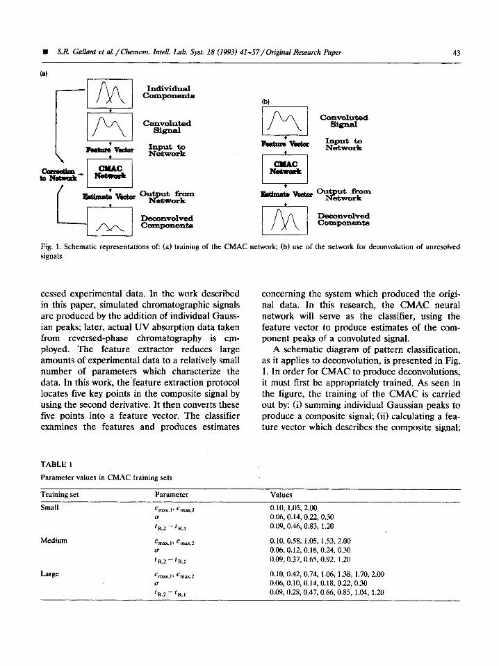
Fig. 1. Schematic repre~ntations of: (a) training signals.

of the CMAC network; (b) use of the network for de~nvolution of unresolved

cessed experimental data. In the work described in this paper, simulated chromatographi~ signals are produced by the addition of individual Gauss- ian peaks; later, actual UV absorption data taken from reversed-phase chromatography is employed. The feature extractor reduces large amounts of experimental data to a relatively small number of parameters which characterize the data. In this work, the feature extraction protocol locates five key points in the composite signal by using the second derivative. It then converts these five points into a feature vector. The classifier examines the features and produces estimates

concerning the system which produced the original data. In this research, the CMAC neural network will serve as the classifier, using the feature vector to produce estimates of the component peaks of a convoluted signal.

A schematic diagram of pattern classification, as it applies to deconvolution, is presented in Fig. 1. In order for CMAC to produce de~nvolutions, it must first be appropriately trained. As seen in the figure, the training of the CMAC is carried out by: (i> summing individual Gaussian peaks to produce a composite signal; (ii> calculating a feature vector which describes the composite signal;

TABLE I

Parameter values in CMAC training sets

Training set

Small

Medium

Large

Parameter Values

cnxlx.1~ =max,z 0.10, 1.05,2.00 a 0.06, 0.14,0.22,0.30 lR.2 - tR.I 0.09,0.46,0.83, 1.20

cnl,x.1* cnlax.2 0.10,0.58, 1.05, 1.53,2.00 u 0.06, 0.12, 0.18, 0.24, 0.30 ?R.2 - fR,I 0.09,0.37,0.65,0.92, 1.20

cnl,x.l~ %lax.2 0.10,0.42, 0.74, 1.06, 1.38, 1.70, 2.00 0 0.06,0.10,0.14,0.18, 0.22,0.30 ‘R.2 - ‘R.1 0.09,0.2x, 0.47,0.66,0.85, 1.04, 1.20

44 S. R. Gallant et al. / Chemom. Intell. Lab. Syst. 18 (I 993) 41-57/ Original Research Paper n

(iii) estimating the deconvolution of the composite signal; and (iv) modifying the network based on the deviation of CMAC’s estimate from the correct deconvolution. Each step in this training sequence is described in detail below. Once training is complete, the network is then employed for deconvolution of a wide range of unknown composite peaks as depicted in Fig. lb.

Chromatographic signal generation

The chromatographic data employed in these computer experiments were generated using the analytical expression for the Gaussian distribution [193.

cj = c max,j exp { -f[(tR,j-‘)/~]z) (1)

where cj is the concentration of the jth peak at time t; c,,,,~ is the peak height; fRIj is the retention time of the peak; t is time; and gj is the standard deviation of the peak. For the purposes of this study, the units of time and concentration are arbitrary. The values of cmax,,, cmax,.+ u, and

tR,2 - tR,l listed in Table 1 were combined to create a ‘smail’, ‘medium’ and ‘large’ training set of composite peaks used to train CMAC for deconvolution.

Feature extraction

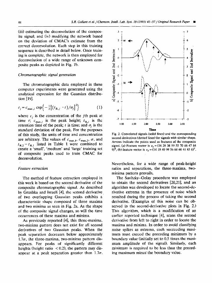
The method of feature extraction employed in this work is based on the second derivative of the composite chromatographic signal. As described by Grushka and Israeli 141, the second derivative of two overlapping Gaussian peaks exhibits a characteristic shape composed of three maxima and two minima as seen in Fig. 2a. As the shape of the composite signal changes, so will the time occurrences of these maxima and minima.

As previous!y reported [4], this three-maxima, two-minima pattern does not exist for all second derivatives of two Gaussian peaks. When the peak separation decreases below approximately 1.7a, the three-maxima, two-minima pattern disappears. For peaks of significantly different heights (height ratio < 0.21, the pattern may dis- appear at a peak separation greater than 1.7~.

3,

2

-6

: I :

1.00 150 2.00 2.50 3.00 3.50

Time

Fig. 2. Convoluted signals (solid lines) and the corresponding second derivatives (dotted fines) for signals with similar shape. Arrows indicate the points used as features of the composite signal. (a) Feature vector is s, = (18 28 38 99 55 70 66 47 84 SIT; (bf feature vector is s2 = (14 18 40 99 56 68 68 41 85 61T,

Nevertheless, for a wide range of peak-height ratios and separations, the three-maxima, two- minima pattern prevails.

The Savitzky-Golay procedure was employed to obtain the second derivatives [20,211, and an algorithm was developed to locate the second-derivative extrema in the presence of noise which resulted during the process of taking the second derivative. (Examples of this noise can be observed in the second-derivative plots in Fig. 2.) This algorithm, which is a modification of an earlier reported technique [4], scans the second derivative from left to right in order to locate the maxima and minima. In order to avoid classifying noise spikes as extrema, each succeeding maximum must exceed the preceding minimum by a boundary value (initially set to 0.5 times the maximum amplitude of the signal). Similarly, each minimum is required to be less than the preceding maximum minus-the boundary value.

w S.R Gallant et al. /Chemom. Intell. Lab. Syst. I8 (1993) 41-57/Origbd Research Paper 45

If the characteristic pattern is not found, the boundary value is halved or doubled (depending on whether too few or too many extrema have been located). This process is repeated until the algorithm succeeds in locating the five maxima and minima. If the algorithm does not detect the characteristic three-maxima, two-minima pattern within ten iterations (because the composite signal is of extremely low resolution or because it has baseline resolution), the signal is discarded from the training set. As a result, the combinations of the parameters listed in Table 1 produced smaller training sets than would be obtained if all of the generated signals were employed. The actual sizes of the small, medium, and large training sets were 47, 225, and 832, respectively. The main difference between this and the earlier reported algorithm is that the boundary ‘floats’. As a result, it will always locate the characteristic pattern if the noise is of lower magnitude than the minimum amplitude of the second derivative.

As seen in Fig. 2, ten features are taken from each composite signal: the time occurrence of the five second-derivative maxima and minima (t,, t,, t,, t,, ts) and the concentration of the original signal at those five times (ci, c2, c3, cd, cJ. The feature extractor uses these values to produce a feature vector according to Eqn. 2:

round(d * [(t, - t,)/w])

round(d * WC,,,))

si = (2)

round(d * [it5 - t,)/w])

round@ * WC,,,))

where si is the feature vector; d is the discretization (the number of integer values that each element in si can assume); t, is the nth time-occurrence feature; c, is the nth concentration feature; t, is the breakthrough time of the composite signal; w is the length of the composite signal (time units); and c,,, is the maximum concentration of the composite signal.

Eqn. 2 represents a scaling process during which the feature times and concentrations are normalized to the magnitude and length of the

signal. This scaling process produces a vector si composed of integer elements ranging in value from 0 to d - 1. Significantly, si has the useful property of depending only on the shape of the composite signal. This shape dependence can be seen in the similarity of the feature vectors presented in the legend of Fig. 2.

Since si is a scaled vector, the output vector yi which contains the parameters of the two, underlying, Gaussian peaks shown in Eqn. 3.

(al/w) Yi =

CC lllC4X,2/Clllt3X >

I Nt,,, - ttJ/w (9/w)

\

1

I I

must also be scaled as

(3)

where yi is the vector to be stored in CMAC; C max,j is the height of the jth component peak; C max is the maximum height of the composite signal; tqj is the retention time of the jth component peak; t, is the breakthrough time of the composite signal; cj is the standard deviation of the jth component peak; and w is the length of the composite signal. The vector yi is not dis- cretized because the actual values calculated using Eqn. 3 (not a discrete approximation) are stored in the CMAC as will be shown below.

As described below, the CMAC network con- sists of the mapping of the scaled feature vector si to the scaled output vector yi. In order to recover the values of c,,, i, c,,, z, tR,,, t, *, and U, the output yi must be unscaled. Since CMAC provides the vector yi and since the height of the composite signal c,,, , its width w, and its breakthrough time t, are known, Eqn. 3 can be solved for the unknown values cmax,i, c,,,~~,~, tR,,, tR,2, and u.

CMAC neural network

The CMAC mapping from the input vector si to the output vector yi is depicted in the set-oriented block diagram Fig. 3a 1171. CMAC creates a mapping from an input vector si to a set of c

46 S.R. Gallant et al. / Chemom. Intel. Lab. Syst. 18 (1993) 41-.57/0riginal Research Paper n

(a) lb) 0

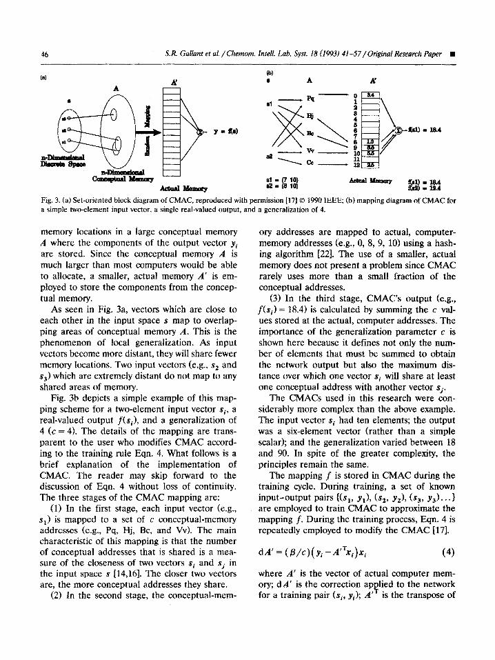
Fig. 3. (a) Set-oriented block diagram of CMAC, reproduced with permission [17] Q 1990 IEEE; (b) mapping diagram of CMAC for a simple two-element input vector, a single real-valued output, and a generalization of 4.

memory locations in a large conceptual memory A where the components of the output vector y, are stored. Since the conceptual memory A is much larger than most computers would be able to allocate, a smaller, actual memory A’ is employed to store the com~nents from the conceptual memory.

As seen in Fig. 3a, vectors which are close to each other in the input space s map to overlapping areas of conceptual memory A. This is the phenomenon of local generalization. As input vectors become more distant, they will share fewer memory locations. Two input vectors (e.g., s2 and sJ) which are extremely distant do not map to any shared areas of memory.

Fig. 3b depicts a simple example of this mapping scheme for a ho-element input vector sj, a real-valued output f(si), and a generalization of 4 (c = 4). The details of the mapping are trans- parent to the user who modifies CMAC according to the training rule Eqn. 4. What follows is a brief explanation of the implementation of CMAC. The reader may skip forward to the discussion of Eqn. 4 without loss of continuity. The three stages of the CMAC mapping are:

(1) In the first stage, each input vector (e.g., s,) is mapped to a set of c conceptual-memory addresses (e.g., Pq, Hj, Bc, and Vv). The main characteristic of this mapping is that the number of conceptual addresses that is shared is a mea- sure of the closeness of two vectors si and sj in the input space s 114,161. The closer two vectors are, the more conceptual addresses they share.

(2) In the second stage, the conceptual-mem-

ory addresses are mapped to actual, computer- memory addresses (e.g., 0, 8, 9, 10) using a hash- ing algorithm [22]. The use of a smaller, actual memory does not present a problem since CMAC rarely uses more than a small fraction of the conceptual addresses.

(3) In the third stage, CMAC’s output (e.g., f(si) = 18.4) is calculated by summing the c values stored at the actual, computer addresses. The importance of the generalization parameter c is shown here because it defines not only the number of elements that must be summed to obtain the network output but also the maximum dis- tance over which one vector si will share at least one conceptual address with another vector sj.

The CMACs used in this research were con- siderably more complex than the above example. The input vector si had ten elements; the output was a six-element vector (rather than a simple scalar); and the generalization varied between 18 and 90. In spite of the greater complexity, the principles remain the same.

The mapping f is stored in CMAC during the training cycle. During training, a set of known input-output pairs KS,, y,), (sZ, y&, ($a, yJ.. .I are employed to train CMAC to appro~mate the mapping f. During the training process, Eqn. 4 is repeatedly employed to modify the CMAC [17].

dA’= (fi/~)(y~-A’~+ (4)

where A’ is the vector of actual computer memory; dA’ is the correction applied to the network for a training pair (si, y,); _4jT is the transpose of

l S.R. Gallant et al. /Chemom. Inteil. Lab. Syst. 18 (1993) 41-57/Original Research Paper 47

A’; yi is the desired network output for a given input si; xi is a binary selection vector; /3 is the training rate; and c is the generalization.

The elements of the vector xi have the value 0 or 1. Those elements which have a value of 1 correspond to the c elements of A’ which must be summed to produce a given network output A’=& If the output is in error, the correction applied to the efements is determined by multiplying the error (yi - JI’~&> by the ratio p/c. The resulting correction is added to each of the summed elements to correct the network at the training point si. Training continues until the average value of dA’ decreases below some threshold, at which time the network is said to have converged.

During the training process, the learning rate of CMAC is controlled by the parameter p. For a training rate p of 0, no change is made in the network. For a training rate of 1, the network is corrected to produce the exact desired output. At the beginning of training, fi is usually set to 1 in order to bring the network to a close approximation of f as soon as possible. In the last phase of training, reduction of p below 1 may help the network to converge in areas of steep functional gradient. In these studies, the CMAC was found to be relatively insensitive to /3 values and a constant value of 1 was employed.

An important feature of CMAC is that it facilitates detection of inadequate training. If, prior to training, each element of A’ is set to an arbitrary, large integer value, the elements which have never been modified during the training can be readily excluded from the output sum. In addition, the fraction of memory locations which have actually been affected by training can be calculated. Thus, an invalid output (i.e., an output in which this fraction does not exceed some threshold) can be discarded, used with a warning, or adjusted by multiplying by the inverse of the fraction of occupied memory locations.

IMPLEMENTATION

The computer programs employed in this paper were written in the LISP programming lan-

guage using the Common LISP Object System (CLOS) [23,24]. The LISP interpreter was purchased from Gold Hill Inc. (Cambridge, MA). This language was chosen because LISP’s auto- matic memory management and Gold Hill’s programming environment significantly shortened program development time. The programs were run on a CC1 33-MHz personal computer with the 80386 processing unit.

As described above, the program included modules for signal processing, feature extraction, and the CMAC network. An object-oriented protocol based on QuickSig 1251 was employed to store and carry out basic operations on the chromatographic signals. This signal processing protocol allowed efficient manipulation of the chromatographic data. The data was stored within computer arrays. The sampling interval was fully adjustable. Operations such as addition, subtrac- tion, scaling, and taking derivatives of signals were defined within the package. Because the signals were defined within a windowing environment, visual monitoring of the signal processing operations was possible and greatly facilitated software development. Data generated in this study were exported to text files and imported into the Microsoft Excel spreadsheet program for analysis.

The implementation of CMAC used in this research generated bit strings as its conceptual- memory addresses. These strings were converted into floating-point numbers and hashed into the LISP data structure for a hash table. The developed CMAC was capable of generating its results in a fraction of a second and of training over a period of minutes to hours depending on the training set size. As an example, training a CMAC with training set size = 47, discretization = 100, generalization = 70, and training passes = 4 required 24 min.

EXPERIMENTAL

Materials

N-Benzoyl-r_.-arginine ethyl ester (Bz-Arg-OEt) and N-benzoyl-t_-alanine (Bz-Ala) were pur-

48 S.R. Gallant et al. /Chemom. Intell. Lab. Syst. 18 (1993) 41-57/0riginal Research Paper w

0.5-l : : : : : : : : 1

0 loll 200 300 400 500 600 700 800 900

Points in Training Set

t

0.5

I 0.5

-r I

0 1 2 3 4

Passes ThroughTraining Set

i--

0 25 50 75 100 0.0 0.5 1.0 IL.5 2.0 2.5

Dfscretization Generalization/Discretization

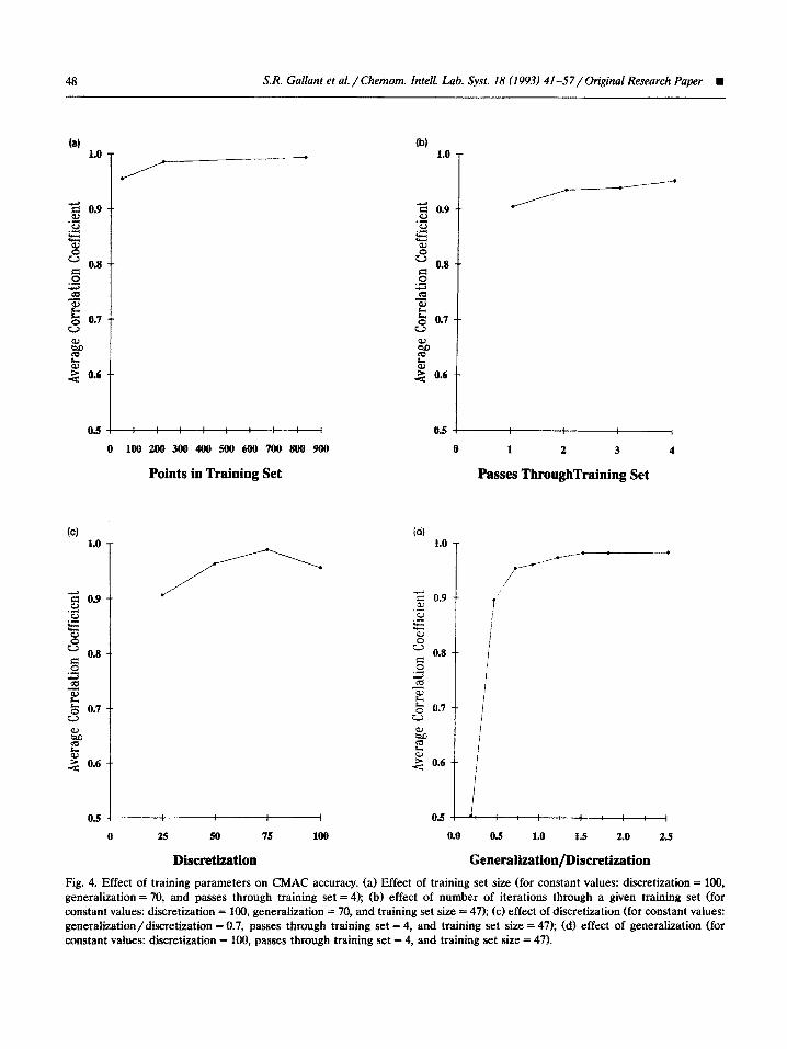
Fig. 4. Effect of training parameters on CMAC accuracy. (a) Effect of training set size (for constant values: discretization = 100, generalization = 70, and passes through training set = 4); (b) effect of number of iterations through a given training set (for constant values: discretization = 100, generalization = 70, and training set size = 47); (c) effect of discretization (for constant values: generai~ation/di~retization = 0.7, passes through training set = 4, and training set size = 47); fd) effect of generalization (for constant values: discretization = 100, passes through training set = 4, and training set size = 47).

W S.R Gallant et al. /Chemom. Intell. Lab. Syst. 18 (1993) 41-57/Original Research Paper 49

chased from Sigma Chemical Company (St. Louis, MO). HPLC-grade acetonitrile and sodium phosphate monobasic were purchased from Fisher Scientific (Rochester, NY). The column (300 x 3.9 mm i.d.1 prepacked with PBondapak octadecyl silica (37-55 pm) was a gift from Waters Chro- matography Division of Millipore Corporation (Milford, MA).

Procedures

The chromatograph employed for these experiments consisted of a Model LC 2150 pump (Pharmacia LKB Biotechnology Inc., Piscataway, NJ) connected to the column via a Model 7125 injector (Rheodyne Inc., Cotati, CA). The column effluent was monitored at 254 nm using a Model 757 Spectroflow UV-VIS detector (Applied Biosystems, Ramsey, NJ). The detector signal was recorded using a Powermate 2 personal computer (NEC Inc., Tokyo, Japan) which was running Maxima 820 data collection software (Waters Chromatography Division, Millipore Corp.). The computer and chromatography software were gifts from Millipore.

In order to produce unresolved signals for deconvolution, the relative concentrations of the two peptides and the organic content of the mobile phase were varied. 20-~1 injections of 0.25 mM Bz-Ala with 0.25, 0.125, or 0.0625 mM Bz- Arg-OEt were used. The chromatograms were recorded under three different mobile phase compositions: 20, 22, and 23% (v/v) acetonitrile in 50 mM sodium phosphate buffer, pH 3.0, to produce varying degrees of peak overlap. In order to verify that the correct deconvolution was produced by CMAC, appropriate solutions of the individual peptides were injected separately into the chromagraph to determine the underlying peaks.

RESULTS AND DISCUSSION

Parametric investigation of CM4C accuracy

The factors controlling the accuracy of the output in the CMAC pattern classifier include: (i)

the number of points in the training set and the distribution of those points across the function surface; (ii) the number of passes made through the training set; and (iii) the discretization and generalization employed in the classifier. The ef- fects of training set size, training iterations, discretization, and generalization on the accuracy of CMAC were evaluated using the correlation coefficient [26].

BY varying cmax,l, c,,,,~, u, and tR,2 - tR,l be-

tween the maximum and minimum values given in Table 1, a test set of random convoluted signals was generated to evaluate the CMAC networks. Correlation coefficients (see Eqn. 5) were then calculated for four of the five parameters estimated by the CMAC (c,,,i, c,,,~~,~, tR,2 and a).

n Cxi’i - ( C’i)( C’i)

r= J-J- (5)

Given pairs of actual and estimated values (x,, i’,), (x2, i:,),..., (x,,, x’,>, Eqn. 4 quantifies the correlation of the observations. For data in which Zi predicts xi strongly, r is near 1.0. For data in which there is no relationship between ii and xi, r is near 0.0. Since the retention time of the first peak, t R ,, testing process, ‘its

was held constant during the correlation coefficient was

mathematically undefined since nCti,,,i = (CtR,,,i)2 and the denominator of Eqn. 5 for this parameter is zero. The remaining four correlation coefficients were averaged to generate an average correlation coefficient. The trends observed in the four individual correlation coefficients were the same as those observed in the average coefficient.

The effect of training set size on the accuracy of estimates returned by CMAC is illustrated in Fig. 4a. As seen in the figure, a training set of 47 composite signals produced a CMAC of relatively high accuracy. As the size of the training set was increased from this value (with the number of training passes held constant), the accuracy slowly increased and asymptotically approached the limit of 1. Two conclusions can be drawn from this result. First, it is possible to attain a good degree

50 S.R. Gallant et al. /Chemom. Intell. Lab. Syst. 18 (1993) 41-57/0riginal Research Paper n

of accuracy with a relatively small training set using this pattern classi~cation system. Second, in order to attain an extremely high degree of accuracy, a relatively large training set will be required.

As training of the CMAC occurs, the values previously stored in the network are changed. Thus, the CMAC does not converge to the most accurate configuration possible during the first pass through the training set. By making repeated passes through the training set, a high degree of accuracy is eventually attained at each training point and at the points between the training points (provided the generalization and discretization are appropriate). The effect of the number of passes through the training set on the accuracy of CMAC is shown in Fig. 4b. While a high degree of accuracy was attained in the first pass through the training set, additional passes resulted in further improvements. Clearly, the accuracy of the CMAC is limited by the specific training set employed (e.g., 47 training points were used to generate Fig. 4b). One of the important features of CMAC is that only a few passes through the training set will usually guarantee convergence.

When the ratio of generalization to discretization is changed, the percent of the network that is affected by each training point is also changed. Thus, in order to examine the effect of discretization alone, it is necessary to hold this ratio constant. Fig. 4c looks at the effect of discretization on the accuracy of CMAC’s output for a constant ratio of generalization to discretization of 0.7. If the discretization is too low, information will be lost because the feature vector will not reflect small changes in the convoluted signal. As the discretization increases, it becomes large enough to adequately represent the system being mapped (e.g., discretization = 75 in Fig. 4~). At high values of discretization, the accuracy of the network can actually decrease due to the greater effect of noise on the CMAC feature vector si. Clearly, the size of the discretization which provides the high- est accuracy will be a function of the size of the training set and the shape of the function surface.

The percent of the network affected by each training point is dete~ined by the ratio of gener-

alization to discretization. Fig. 4d depicts the effect of changing this ratio on the accuracy of the resulting CMAC network. For low vafues of this ratio (e.g., 0.2 in the figure) many areas of the network are effectively isolated. This results in both a minimal number of training points within a given generalization region and a lack of interactions between the regions corresponding to the various training points. As the ratio of generalization to discretization increases, the isolated areas of the network becomes smaller, and the accuracy of the network output is increased. For the deconvolution mapping f, higher values of the generalization continually improved the accuracy of the network. However, for extremely large values of the generalization to discretization ratio, the increased memory requirements would no longer be justified by an increase in network accuracy.

CMAC networks with large memory requirements did not always provide the greatest accuracy. One CMAC trained in this research required 39.1 kilobytes of memory to achieve a correlation coefficient of 0.503 (discretization = 100, generalization = 20, training set size = 47). Another required 18.6 kilobytes to achieve a correlation coefficient of 0.987 (discretization = 75, generalization = 53, training set size = 47). Clearly, appropriate combinations of discretization, generalization, and training size can both dramatically increase the network accuracy and reduce the memory requirements.

As a result of this parametric investigation of CMAC accuracy, the following network parameters were employed to generate a CMAC with an overall correlation coefficient of 0.994: discretization = 100, generalization = 70, training set size = 832, and training passes = 4. This network was trained using the large training set described in Table 1 and was employed for all the deconvolutions described below.

Deconvoiution of simuiuted peaks

Since CMAC allows the variance and heights of the underlying chromatographic peaks to be recovered from the convoluted signal, it is able to produce deconvolved chromatograms from over-

n S.R Gallant et al. /Chemm. IntelL Lab. Syst. 18 (1993) 41-57/Originai Research Paper 51

lapping peaks. In order to assess CMAC’s accd- racy, a variety of composite peaks was deconvolved. CMAC was tested outside the training region covered in Table 1 in order to demonstrate that only the shape and not the magnitude of the composite signal governed the deconvolution process. Of course, the scaled input vectors si produced from the test set would have to correspond to a shape similar to one in the training set or CMAC would not succeed in deconvolving it. However, this method of training will certainly save time and memory space over a method that does not use scaling.

In creating the signals used to test CMAC, the parameters of the first component were held constant (P = 20, cmax,, = 10, and tn,, = 100) while the second component’s height and separation from the first peak were-varied from O.lc,, , to l.Oc max,,, and 1.70 to 4.0a, respectively. Similar deconvolution results were obtained for a set of composite signals in which the parameters of the second peak were held constant and the parameters of the first peak were varied.

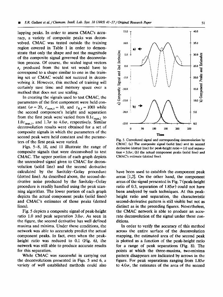
Figs. 5-8, 10, and 11 illustrate the range of composite signals that were deconvolved to test CMAC. The upper portion of each graph depicts the unresolved signal given to CMAC for deconvolution (solid line) and the second derivative calculated by the Savitzky-Golay procedure (dotted line). As described above, the second-derivative noise produced by the Savitzky-Golay procedure is readily handled using the peak scan- ning algorithm. The lower portion of each graph depicts the actual component peaks (solid lines) and CMAC’s estimates of those peaks (dotted lines).

Fig. 5 depicts a composite signal of peak-height ratio 1.0 and peak separation 3.0a. As seen in the figure, the second derivative has well defined maxima and minima. Under these conditions, the network was able to accurately predict the actual component peaks. In fact, even when the peak- height ratio was reduced to 0.1 (Fig. 61, the network was still able to produce accurate results for this separation.

While CMAC was successful in carrying out the deconvolutions presented in Figs. 5 and 6, a variety of well established methods could also

P 3

$ 5.0

‘C e: P

w 0.0

a

8

;a 5.0

GilI a 2 -10.0

P :: -15.0 T

-25.0

0 so 100 150 200 250

Time

Fig. 5, Convoluted signal and corresponding deconvolution by CMAC. (a) The composite signal (solid line) and its second derivative (dotted line) for peak-height ratio = 1.0 and separation = 3.0~; (b) the actual component peaks (solid line) and CMAc’s estimate (dotted line).

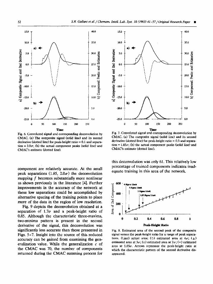
have been used to establish the component peak areas [1,2]. On the other hand, the component areas of the signal presented in Fig. 7 (peak-height ratio of 0.3, separation of 1.85~) could not have been analyzed by such techniques. At this peak- height ratio and separation, the characteristic second-derivative pattern is still visible but not as distinct as in the preceding figures. Nevertheless, the CMAC network is able to produce an accurate deconvolution of the signal under these conditions.

In order to verify the accuracy of this method across the entire surface of the deconvolution mapping, the estimated area of the second peak is plotted as a function of the peak-height ratio for a range of peak separations (Fig. 8). The points at which the three-maxima, two-minima pattern disappears are indicated by arrows in the figure. For peak separations ranging from 1.85~ to 4.Ou, the estimates of the area of the second

S.R. Gallant et al. / Chemom. Intell. Lab. Syst. 18 (1993) 41-57/Original Research Paper n

i

40.0

I.0

A ~ 35.0

30.0 3

E 3

25.0 $

B m

20.0 -8 &

u” -15.0 10.0 s “i;i‘

-20.0 50

-25.0 0.0

0 so 100 150 200 250

Fig. 6. Convoluted signal and corresponding deconvolution by CMAC. (a) The composite signal (solid line) and its second derivative (dotted line) for peak-height ratio = 0.1 and separation = 3.0~; (b) the actual component peaks (solid line) and

Time

CMAC’s estimate (dotted line).

component are relatively accurate. At the small peak separations (1.85, 2.00) the de~nvolutio~ mapping f becomes substantially more nonlinear as shown previously in the literature [4]. Further improvements in the accuracy of the network at these low separations could be accomplished by alternative spacing of the training points to place more of the data in the region of low resolution.

Fig. 9 depicts the deconvolution obtained at a separation of 1.7~ and a peak-height ratio of 0.85. Although the characteristic three-maxima, two-minima pattern is present in the second de~vative of the signal, this de~nvolution was significantly less accurate than those presented in Figs. 5-7. Insight into the source of this reduced accuracy can be gained from examining the generalization value. While the generalization c of the CMAC was 70, the number of components returned during the CMAC su~ing process for

-a B a -5.0

.#

+$ -10.0

B

Fig. 7. Convoluted signal and corresponding deconvolution by CMAC. (a) The composite signal (solid line) and its second

0

derivative (dotted line) for peak-height ratio = 0.3 and separa-

50

tion = 1.85~; (b) the actual ~rn~nent peaks (solid line) and

100

CMAC’s estimate (dotted line).

150 200 250

Time

this deconvolution was only 61. This relatively low percentage of trained components indicates inadequate training in this area of the network.

4 Sigma Limit

0 0.2 0.4 0.6 0.8 1

Pa-Heft Ratio

Fig. 8. Estimated area of the second peak of the composite signal versus the peak-height ratio for a range of peak separations. (Line) actual area; (0) estimated area at 4~; (A) estimated area at 3~; (01 estimated area at 2~; ( *) estimated area at 1.850. Arrows represent the peak-height ratio at which the characteristic pattern of the second derivative dis- appeared.

n S.R. Gallant et al. /Chemom. InteN. Lab. Syst. 18 (1993) 41-57/Origirtal Research Paper 53

15.0

10.0

g 3 .E

5.0

p:

iis O.O -u 9

a -5.0

3

2 ’ w -10.0

i% s -15.0 ‘;;i

\ t t t : : ;-‘._’

t : ‘_’

+

40.0

35.0

30.0 E -z

2

25.0 $

8 m

20.0 % 2

-s 15.0 B

& E

s 10.0 s

5.0

0.0

0 50 100 150 200 2.50

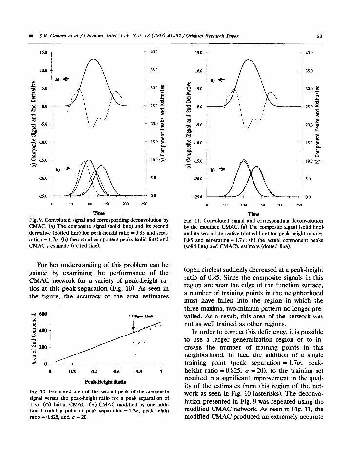
Time Fig. 9. Convoluted signal and corresponding deconvolution by CMAC. (a) The composite signal (solid line) and its second derivative (dotted line) for peak-height ratio = 0.85 and separation = 1.7~; (b) the actual component peaks (solid line) and CMAC’s estimate (dotted line).

Further understanding of this problem can be gained by examining the performance of the CMAC network for a variety of peak-height ratios at this peak separation (Fig. 10). As seen in the figure, the accuracy of the area estimates

0 0.2 0.4 0.6 0.8 1

Peak-Height Ratio

Fig. 10. Estimated area of the second peak-of the composite signal versus the peak-height ratio for a peak separation of 1.7~. to) Initial CMAC, (*) CMAC modified by one additional training point at peak separation = 1.7~; peak-height ratio = 0.825, and (T = 20.

40.0

35.0

30.0 8 t E

3

25.0 4 w B v)

20.0 % B

-s 15.0 s

zi. E u”

10.0 3

5.0

0.0

0 50 100 150 200 250

Time Fig. 11. Convoluted signal and corresponding deconvolution by the modified CMAC. (a) The composite signal (solid line) and its second derivative (dotted line) for peak-height ratio = 0.85 and separation = 1.7~; (b) the actual component peaks (solid line) and ChBAC’s estimate (dotted line).

(open circles) suddenly decreased at a peak-height ratio of 0.85. Since the composite signals in this region are near the edge of the function surface, a number of training points in the neighborh~ must have fallen into the region in which the three-maxima, two-minima pattern no longer pre- vailed. As a result, this area of the network was not as well trained as other regions.

In order to correct this deficiency, it is possible to use a larger generalization region or to increase the number of training points in this neighborhood. In fact, the addition of a single training point (peak separation = 1.7a, peak- height ratio = 0.825, u = 201, to the training set resulted in a significant improvement in the qual- ity of the estimates from this region of the network as seen in Fig, 10 (asterisks). The deconvolution presented in Fig. 9 was repeated using the modified CMAC network. As seen in Fig. 11, the modified CMAC produced an extremely accurate

54 S.R. Gallant et al. / Chemom. Intell. Lab. Syst. 18 (1993) 41-57/Original Research Paper w

de~nvolution. These results clearly demonstrate how inaccuracies in the network can be dramatically improved by appropriate modifications in the training set.

Deconuolution of expetimentul chrornatograrns

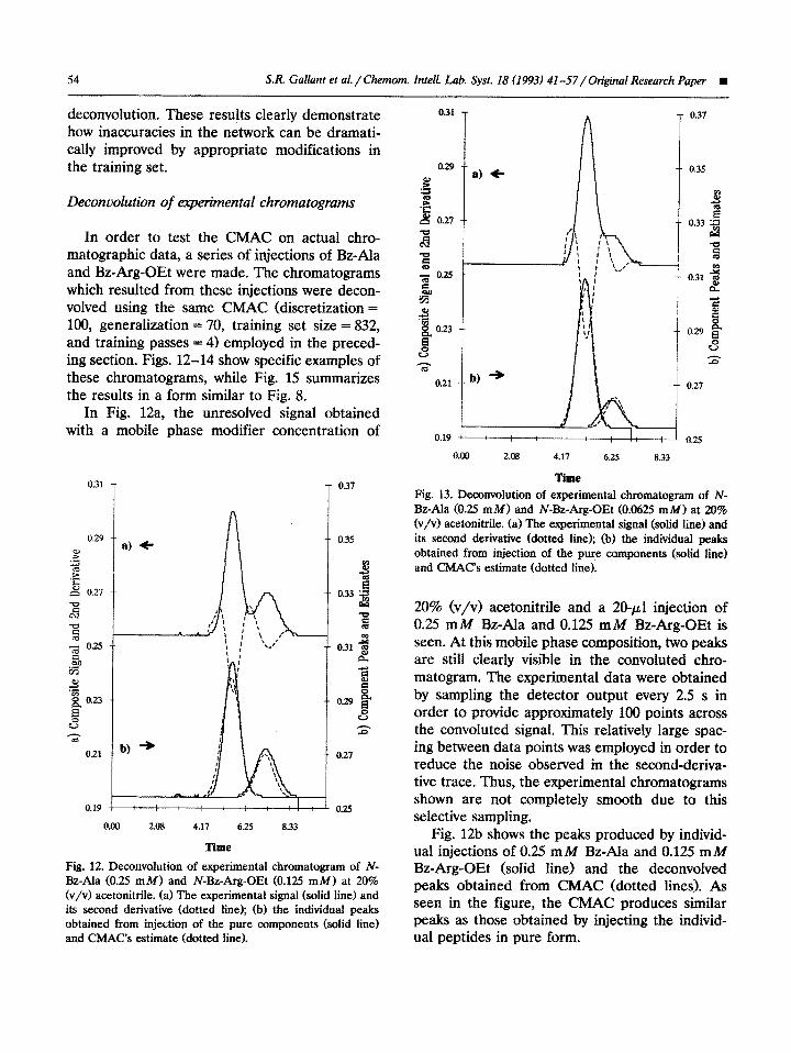
In order to test the CMAC on actual chromatographic data, a series of injections of Bz-Ala and Bz-Arg-OEt were made. The chromatograms which resulted from these injections were deconvolved using the same CMAC (discretization = 100, generalization = 70, training set size = 832, and training passes = 4) employed in the preceding section. Figs. 12-14 show specific examples of these chromatograms, while Fig. 15 summarizes the results in a form similar to Fig. 8.

In Fig. 12a, the unresolved signal obtained with a mobile phase modifier concentration of

0.31 T T 0.37

0.29 0.35

0.25

4.17 6.25 8.33

Time

Fig. 12. Deconvolution of experimental chromatogram of N- Bz-Ala (0.25 mM) and iV-Bz-Arg-OEt (0.125 mM) at 20% (v/v) acetonitrile. (a) The experimental signal (solid line) and its second derivative (dotted line); (b) the individual peaks obtained from injection of the pure components (solid line) and CMAC’s estimate (dotted line).

0.29

g 74

6 0.27

0.19 i

0.00 2.08 4.17

Time

6.2s 8.33

Fig. 13. Deconvolution of experimental chromatogram of N- Bz-Ala (0.25 m&f) and N-Bz-Arg-OEt (0.0625 mM) at 20% (v/v) acetonitrile. (a) The experimental signal (solid line) and its second derivative (dotted line); (b) the individual peaks obtained from injection of the pure ~m~nents (solid line) and CMAC’s estimate (dotted line).

20% (v/v> acetonitrile and a 20-~1 injection of 0.25 mM Bz-Ala and 0.125 mM Bz-Arg-OEt is seen. At this mobile phase composition, two peaks are still clearly visible in the convoluted chromatogram. The experimental data were obtained by sampling the detector output every 2.5 s in order to provide appro~mately 100 points across the convoluted signal. This relatively large spacing between data points was employed in order to reduce the noise observed in the second-derivative trace. Thus, the experimental chromatograms shown are not completely smooth due to this selective sampling,

Fig. 12b shows the peaks produced by individual injections of 0.25 mild Bz-Ala and 0.125 mM Bz-Arg-OEt (solid line) and the deconvolved peaks obtained from CMAC (dotted lines). As seen in the figure, the CMAC produces similar peaks as those obtained by injecting the individual peptides in pure form.

8 S.R. Gallant et al./Chemom. Intell. Lab. Syst. 18 (1993) 41-57/0riginal Research Paper 55

0.37

0.27

0.19 0.25

0.00 2.08 4.17 6.25 8.33

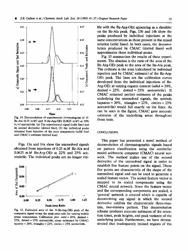
Time Fig. 14. Deconvolution of experimental chromatogram of N- Bz-Ala (0.25 mM) and N-Bz-Arg-OEt (0.0625 mM) at 20% (v/v) acetonitrile. (a) The experimental signal (solid line) and its second derivative (dotted line); (b) the individual peaks obtained from injection of the pure components (solid line) and CMAC’s estimate (dotted line).

Figs. 13a and 14a show the unresolved signals obtained from injections of 0.25 mA4 Bz-Ala and 0.0625 mM Bz-Arg-OEt in 22% and 23% acetonitrile. The individual peaks are no longer visi-

0.00 0.25 0.50 0.75 1.00 1.25

Peak-Area Ratio

Fig. 15. Estimated area of the N-Bz-Arg-(iEt peak of the composite signal versus the peak-area ratio for varying mobile phase composition. Calibration plot: solid = 20%, dashed = 22%, dotted = 23% acetonitrile; areas estimated by CMAC: squares = 20%, triangles = 22%, circles = 23% acetonitrile.

ble with the Bz-Arg-OEt appearing as a shoulder on the Bz-Ala peak. Figs. 13b and 14b show the peaks produced by individual injections at the same concentrations as those present in the mixed solution (solid lines). In both cases, the deconvolution produced by CMAC (dotted lines) well approximates these individual peaks.

Fig. 15 summarizes the results of these experiments. The abscissa is the ratio of the area of the Bz-Arg-OEt peak to the area of the Bz-Ala peak. The ordinate is the area (calculated by individual injection and by CMAC estimate) of the Bz-Arg- OEt peak. The lines are the calibration curves developed from the individual injections of Bz- Arg-OEt at varying organic content (solid = 20%, dashed = 22%, dotted = 23% acetonitrile). If CMAC returned perfect estimates of the peaks underlying the unresolved signals, the symbols (squares = 20%, triangles = 22%, circles = 23% acetonitrile) would fall exactly on the lines. As can be seen in the figure, CMAC gave accurate estimates of the underlying areas throughout these tests.

CONCLUSIONS

This paper has presented a novel method of deconvolution of chromatographic signals based on pattern classification using the cerebellar model arithmetic computer (CMAC) neural network. The method makes use of the second derivative of the unresolved signal in order to establish five feature points on the signal. These five points are characteristic of the shape of the unresolved signal and can be used to generate a scaled feature vector. The scaled feature vector is mapped to its scaled components using the CMAC neural network. Since the feature vector and the corresponding components are scaled, a ‘general’ network is created which is capable of deconvolving any signal in which the second derivative exhibits the characteristic three-maxima, two-minima pattern. This deconvolution scheme produces accurate estimates of the retention times, peak heights, and peak variance of the underlying peaks. Furthermore, we have demon- strated that inadequately trained regions of the

56 S.R. Gallant et al. / Chemom. Intell. Lab. Syst. 18 (1993) 41-57/Original Research Paper n

network can be dramatically improved by the addition of appropriate training points. Once the CMAC network is established using an appropriate training procedure, the system is able to provide rapid, constant-time deconvolutions of both simulated and actual chromatographid signals.

While the signals employed in this paper were composed of Gaussian peaks, the applications of CMAC for chromatographic deconvolution should not be viewed as so tightly constrained. In fact, it should be possible to deconvolve composite signals composed of a wide variety of distributions. This is an important advantage of the use of CMAC over other possible methods of unresolved peak area estimation. We are presently creating CMAC networks trained using the log- normal and other distributions which more aceu- rately describe the peak shapes observed in real analytical and preparative chromatographic applications [91.

SYMBOLS

A A’ A

A’

C

‘j

cn C mm

C mahi

f” si t

tb

t”

‘RJ

W

ni

Yi

Conceptual CMAC memory Actual CMAC memory Vector representation of conceptual CMAC memory Vector representation of actual CMAC memory CMAC generalization Concentration of jth component at a par- ticular time Concentration at nth feature point Maximum concentration of signal Maximum concentration of jth component CMAC discretization Mapping stored in CMAC Feature vector i Time Breakthrough time Time at nth feature point Retention time of jth component Length of signal Binary selection vector Output vector corresponding to feature vector i

P CMAC training rate

5 Standard deviation of jth component

ACKNOWLEDGEMENTS

This investigation was supported by a National Science Foundation Grant No. CTS-8957746 (Presidential Young Investigation Award to SMC) and by Millipore Corporation.

REFERENCES

1

2

3

4

5

6

7

8

A.W. Westerberg, detection and resolution of overlapping peaks for an on-line computer system for gas chro- matographs, Analytical Chemistry, 41 (1969) 1770-1777.

A. Fozard, J.J. Frances and A.J. Wyatt, Real-time peak detection and area apportionment of unknown chromatograms, Chromatographia, 5 (1972) 130-135. E. Grushka and I. Atamna, The use of derivatives for establishing integration limits of chromatographic peaks, Chromatographia, 24 (1987) 226-232.

E. Grushka and D. Israeli, Characterization of overlapped chromatographic peaks by their second derivative, the limit of the method, Analytical Chemistry, 62 (1990) 717- 721. A.H. Anderson, T.C. Gibb and A.B. Littlewood, Com- puter analysis of unresolved non-Gaussian gas chromatograms by curve-fitting, Analytical Chemistry, 42 (1970)

434-440. R.A. Vaidya and R.D. Hester, Deconvolution of overlapping chromatographic peaks using constrained non-linear optimization, Journal of Chromatography, 287 (1984) 231-

244. P.J.H. Scheeren, Z. Klaus and H.C. Smit, A software package for the orthogonal polynomial approximation of analytical signals, including a simulation program for chromatograms and spectra, Analytica Chimica Acta, 171(1985)

45-60. R.A. Caruana, R.B. Searle, T. Heller and S.I. Shupack, Fast algorithm for the resolution of spectra, Analytical

Chemdy, 58 (1986) 1162-1167. J. Grimalt, H. Iturriaga and J. Olive, An experimental study of the efficiency of different statistical functions for the resolution of chromatograms with overlapping peaks, Analytica Chimica Acta, 201 (1987) 193-205.

K. Kalghatgi and C. Horvath, Rapid peptide mapping by high-performance liquid chromatography, Journal of Chro- matography, 443 (1988) 343-354. R.P. Lippmann, Pattern classification using neural networks, IEEE Communications Magazine, 27 (1989) 47-64.

L.H. Ungar, B.A. Powell and S.N. Kamens, Adaptive networks for fault diagnosis and process control, Comput-

ers in Chemical Engineering, 14 (1990) 561-572.

n S.R. Gallanr et al. /&morn. Inrell. Lab. Syst. 18 (1993) 41-57/Original Research Paper 57

13 D. Logan and P. Argyrakis, Neural Nets for Eliminating

Noise in Experimental Signals, IBM Corporation, Scientific and Engineering Computations Department 48B/428, Kingston, NY, 1990.

14 J.S. Albus, A new approach to manipulator control: the cerebellar model articulation controller, Journal of Dy- namic Systems, Measurement, and Control, 97 (1975) 220-

227. 15 J.S. Albus, Data storage in the cerebellar model articula-

tion controller (CMAC), Journal of Dynamic Systems, Measurement, and Conrrol, 97 (1975) 228-233.

16 J.S. Albus, Brain, Behacior, and Robotics, Byte Books, Peterborough, NH, 1981.

20

21

22

23

24

17 W.T. Miller, F.H. Glanz and L.G. Kraft, CMAC: an asso- ciative neural network alternative to backpropagation, Proceedings of the IEEE, 78 (1990) 1561-1567.

18 R.O. Duda and P.E. Hart, Pattern Classification and Scene Analysis, Wiley, New York, 1973.

19 C. Horvath and W. Melander, Theory of chromatography, in E. Heftmann (Editor), Chromatography: Fundamentals and Applications of Chromarographic and Electrophoretic Methods, Elsevier, Amsterdam, 1983.

25

26

A. Savitzky and M.J.E. Golay, Smoothing and differentiation of data by simplified least squares procedures, Analyt- ical Chemistry, 36 (1964) 1627-1639.

J. Steinier, Y. Termonia and J. Deltour, Comments on smoothing and differentiation of data by simplified least square procedure, Analytical Chemistry, 44 (1972) 1906- 1909.

R. Sedgewick, Algorithms, Addison-Wesley, Reading, MA, 1983. R. Wilensky, Common LISPcraft, Norton and Company, New York, 1986. S. Keene, Object-Oriented Programming in Common Lisp,

Addison-Wesley, Reading, MA, 1989. M. Karjalainen, T. Altosaar and P. Alku, QuickSig - An object-oriented signal processing environment, Proceidings

of the Inrernational Conference on Acoustics, Speech, and

Signal Processing, 3 (1988) 1682-1685. J. Devore, Probability and SIatistics for Engineering and the

Sciences, Brook/Cole, Monterey, CA, 1987.

Documents

Deconvolution of overlapping chromatographic peaks using a cerebellar model arithmetic computer neural network