Curves: Definition and Types | Curves| Surveying

Definition of Curves:

Curves are regular bends provided in the lines of communication like roads, railways

etc. and also in canals to bring about the gradual change of direction. They are also

used in the vertical plane at all changes of grade to avoid the abrupt change of grade

at the apex.

Curves provided in the horizontal plane to have the gradual change in direction are

known as Horizontal curves, whereas those provided in the vertical plane to obtain

the gradual change in grade are known as vertical curves. Curves are laid out on the

ground along the centre line of the work. They may be circular or parabolic.

Classification of Curves:

(i) Simple,

(ii) Compound

(iii) Reverse and

(iv) Deviation

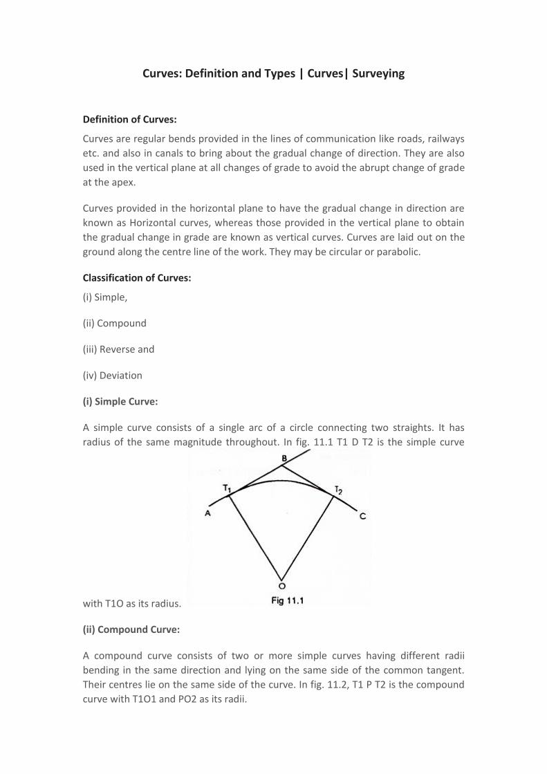
(i) Simple Curve:

A simple curve consists of a single arc of a circle connecting two straights. It has

radius of the same magnitude throughout. In fig. 11.1 T1 D T2 is the simple curve

with T1O as its radius.

(ii) Compound Curve:

A compound curve consists of two or more simple curves having different radii

bending in the same direction and lying on the same side of the common tangent.

Their centres lie on the same side of the curve. In fig. 11.2, T1 P T2 is the compound

curve with T1O1 and PO2 as its radii.

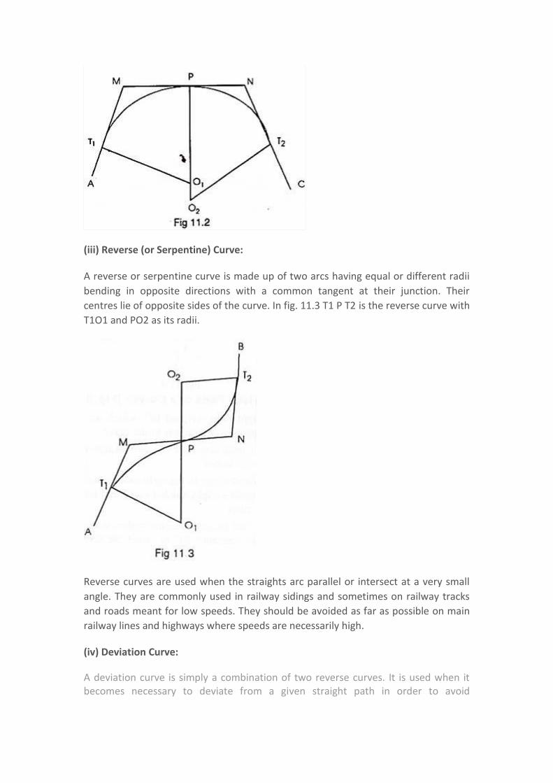
(iii) Reverse (or Serpentine) Curve:

A reverse or serpentine curve is made up of two arcs having equal or different radii

bending in opposite directions with a common tangent at their junction. Their

centres lie of opposite sides of the curve. In fig. 11.3 T1 P T2 is the reverse curve with

T1O1 and PO2 as its radii.

Reverse curves are used when the straights arc parallel or intersect at a very small

angle. They are commonly used in railway sidings and sometimes on railway tracks

and roads meant for low speeds. They should be avoided as far as possible on main

railway lines and highways where speeds are necessarily high.

(iv) Deviation Curve:

A deviation curve is simply a combination of two reverse curves. It is used when it becomes necessary to deviate from a given straight path in order to avoid

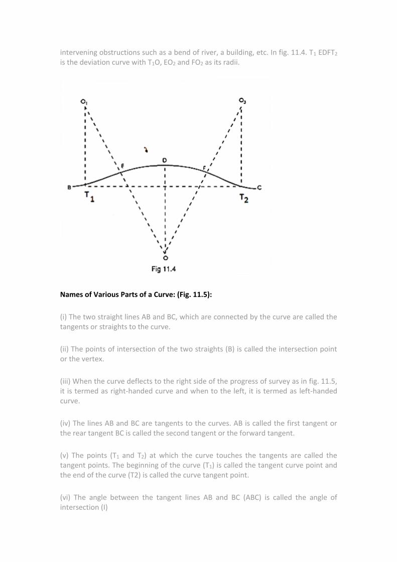
intervening obstructions such as a bend of river, a building, etc. In fig. 11.4. T1 EDFT2 is the deviation curve with T1O, EO2 and FO2 as its radii.

Names of Various Parts of a Curve: (Fig. 11.5):

(i) The two straight lines AB and BC, which are connected by the curve are called the tangents or straights to the curve.

(ii) The points of intersection of the two straights (B) is called the intersection point or the vertex.

(iii) When the curve deflects to the right side of the progress of survey as in fig. 11.5, it is termed as right-handed curve and when to the left, it is termed as left-handed curve.

(iv) The lines AB and BC are tangents to the curves. AB is called the first tangent or the rear tangent BC is called the second tangent or the forward tangent.

(v) The points (T1 and T2) at which the curve touches the tangents are called the tangent points. The beginning of the curve (T1) is called the tangent curve point and the end of the curve (T2) is called the curve tangent point.

(vi) The angle between the tangent lines AB and BC (ABC) is called the angle of intersection (I)

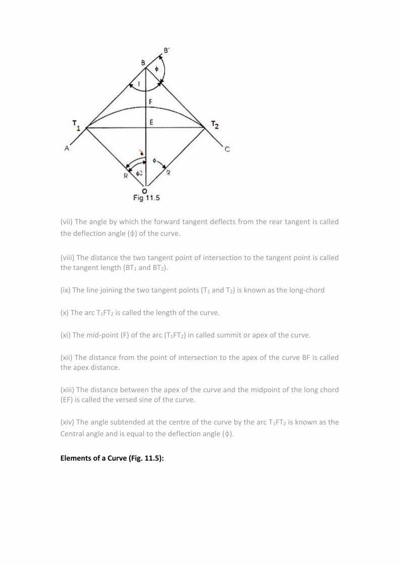
(vii) The angle by which the forward tangent deflects from the rear tangent is called

the deflection angle (ɸ) of the curve.

(viii) The distance the two tangent point of intersection to the tangent point is called the tangent length (BT1 and BT2).

(ix) The line joining the two tangent points (T1 and T2) is known as the long-chord

(x) The arc T1FT2 is called the length of the curve.

(xi) The mid-point (F) of the arc (T1FT2) in called summit or apex of the curve.

(xii) The distance from the point of intersection to the apex of the curve BF is called the apex distance.

(xiii) The distance between the apex of the curve and the midpoint of the long chord (EF) is called the versed sine of the curve.

(xiv) The angle subtended at the centre of the curve by the arc T1FT2 is known as the

Central angle and is equal to the deflection angle (ɸ).

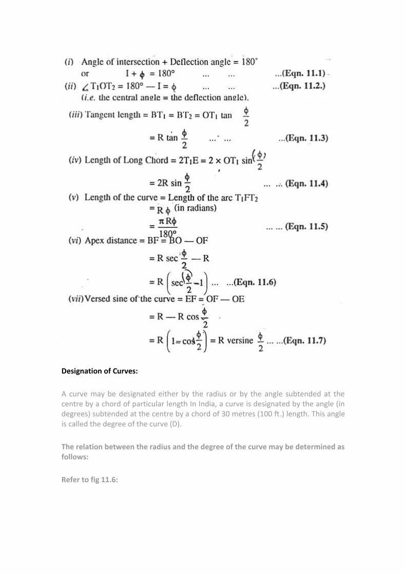
Elements of a Curve (Fig. 11.5):

Designation of Curves:

A curve may be designated either by the radius or by the angle subtended at the centre by a chord of particular length In India, a curve is designated by the angle (in degrees) subtended at the centre by a chord of 30 metres (100 ft.) length. This angle is called the degree of the curve (D).

The relation between the radius and the degree of the curve may be determined as follows:

Refer to fig 11.6:

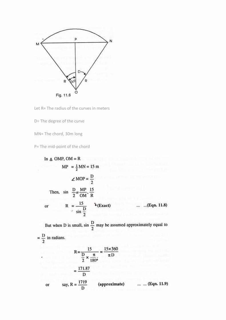
Let R= The radius of the curves in meters

D= The degree of the curve

MN= The chord, 30m long

P= The mid-point of the chord

The approximate relation holds good up to 5° curves. For higher degree curves,

the exact relation should be used.

Methods of Curve Ranging:

A curve may be set out:

1. By linear methods, where chain and tape are used.

2. By angular or instrumental methods, where a theodolite with or without a chain is used.

Before starting setting out a curve by any method, the exact positions of the tangent points between which the curve lies, must be determined.

For this, proceed as follows: (Fig. 11.5)

(i) Having fixed the directions of the straights, produce them to meet at point (B).

(ii) Set up a theodolite at the intersection point (B) and measure the angle of

intersection (I). Then find the deflection angle (ɸ) by subtracting (I) from 180°. i.e.,

ɸ = 180° — I

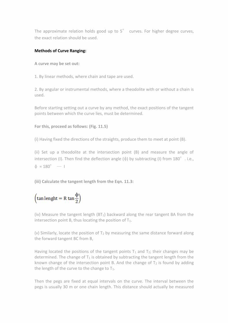
(iii) Calculate the tangent length from the Eqn. 11.3:

(iv) Measure the tangent length (BT1) backward along the rear tangent BA from the intersection point B, thus locating the position of T1.

(v) Similarly, locate the position of T2 by measuring the same distance forward along the forward tangent BC from B,

Having located the positions of the tangent points T1 and T2; their changes may be determined. The change of T1 is obtained by subtracting the tangent length from the known change of the intersection point B. And the change of T2 is found by adding the length of the curve to the change to T1.

Then the pegs are fixed at equal intervals on the curve. The interval between the pegs is usually 30 m or one chain length. This distance should actually be measured

along the arc, but in practice it is measured along the chord, as the difference between the chord and the corresponding arc is small and hence negligible. In order that this difference is always small and negligible, the length of the chord should not be more than 1/20th of the radius of the curve. The curve is then obtained by joining all these pegs.

The distances along the centre line of the curve are continuously measured from the point of beginning of the line up to the end, i.e., the pegs along the centre line of the work should be at equal interval from the beginning of the line to the end. There should be no break in the regularity of their spacing in passing from a tangent to a curve or from a curve to a tangent.

For this reason, the first peg on the curve is fixed at such a distance from the first tangent point (T1) that its change becomes the whole number of chains i.e. the whole number of peg interval. The length of the first chord is thus less than the peg interval and is called as a sub- chord. Similarly, there will be a sub chord at the end of the curve. Thus, a curve usually consists of two-chords and a number of full chords. This is made clear from the following example.

Linear Methods of Setting out Curves

The following are the methods of setting out simple circular curves by linear

methods and by the use of chain and tape: 1. By ordinates from the Long chord 2. By

Successive Bisection of Arcs. 3. By Offsets from the Tangents. 4. By Offsets from

Chords Produced.

Method # 1. By Ordinates from the Long Chord (Fig. 11.8):

Let T1T2=L= the length of the Long chord

ED= O0= the offset at mid-point (e) of the long chord (the versed sine)

PQ=Ox= the offset at distance x from E

Draw QQ1 parallel to T1 T2 meeting DE at Q1

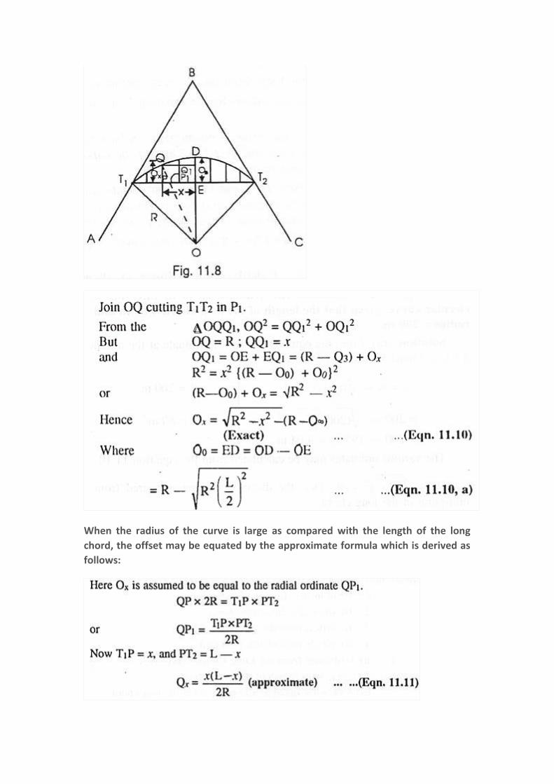
When the radius of the curve is large as compared with the length of the long

chord, the offset may be equated by the approximate formula which is derived as

follows:

Note:

In the exact equation (11.1), the distance x of the point P is measured from the

mid-point of the long chords; while in the approximate equation (11.11), it is

measured from the first tangent point (T1).

Procedure of Setting Out the Curve:

(i) Divide the long chord into an even number of equal parts.

(ii) Calculate the offsets by the equation 11.10 at each of the points of division.

Note:

1. Since the curve is symmetrical on both sides of the middle- ordinate, the offsets

for the right-hand half of the curve are the same as those for the left-hand half.

ADVERTISEMENTS:

2. If the offsets are found by the approximate equation (11.11), the long chord

should be divided into a convenient number of equal parts and the calculated offsets

laid out at each of the points of division.

This method is used for setting out short curves e.g., curves for street bends.

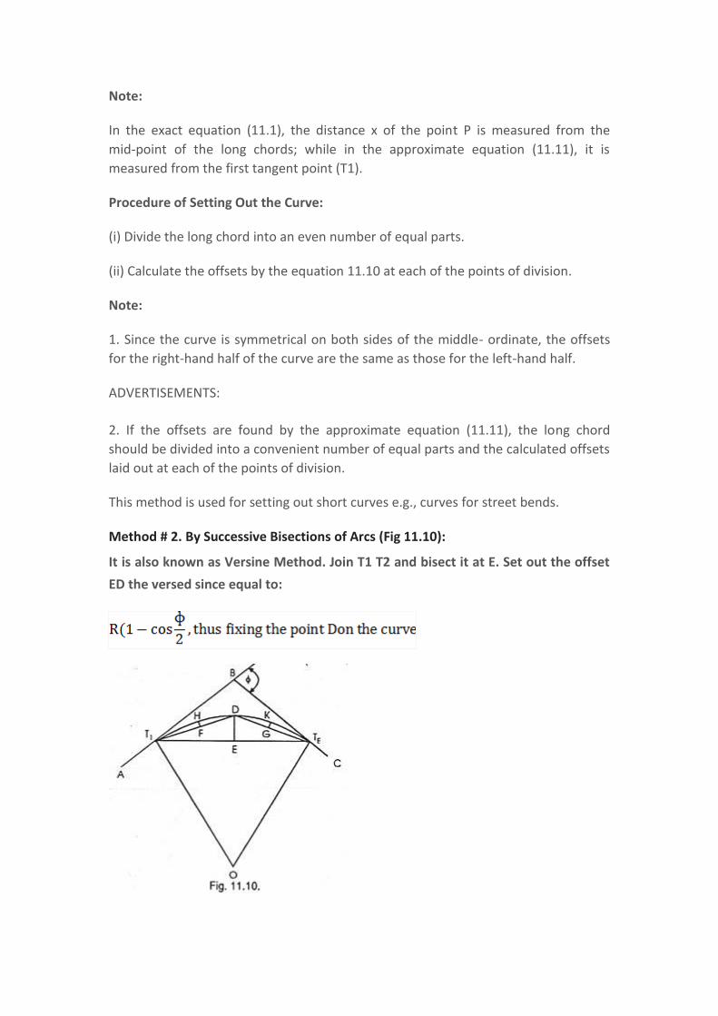
Method # 2. By Successive Bisections of Arcs (Fig 11.10):

It is also known as Versine Method. Join T1 T2 and bisect it at E. Set out the offset

ED the versed since equal to:

Join T1D and DT2 and bisect them at F and G respectively. Then set outsets FH and

GK at F and G each equal to thus fixing two more points H and K on

the curve. Then each of the offsets to be set out at mid points of the chords T1H, HD,

DK and KT2 is equal to .By repeating this process, set out as many

point as are required.

This method is suitable where the ground outside the curve is not favorable to the

tangents.

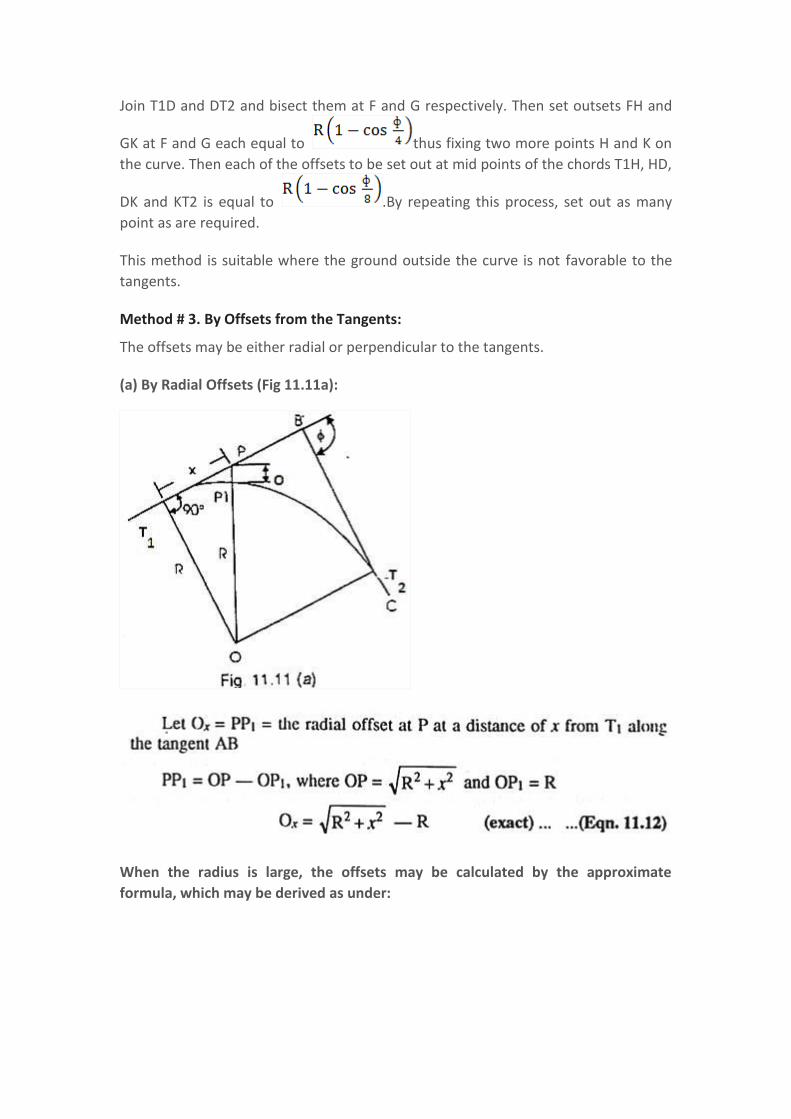
Method # 3. By Offsets from the Tangents:

The offsets may be either radial or perpendicular to the tangents.

(a) By Radial Offsets (Fig 11.11a):

When the radius is large, the offsets may be calculated by the approximate

formula, which may be derived as under:

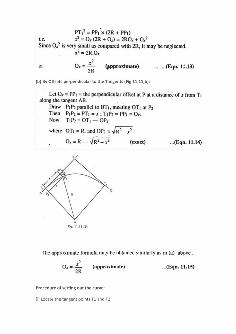
(b) By Offsets perpendicular to the Tangents (Fig 11.11,b):

Procedure of setting out the curve:

(i) Locate the tangent points T1 and T2.

(ii) Measure equal distances, say 15 or 30 m along the tangent from T1.

(iii) Set out the offsets calculated by any of the above methods at each distance, thus

obtaining the required points on the curve.

(iv) Continue the process until the apex of the curve is reached.

(v) Set out the other half of the curve from the second tangent.

This method is suitable for setting out sharp curves where the ground outside the

curve is favourable for chaining.

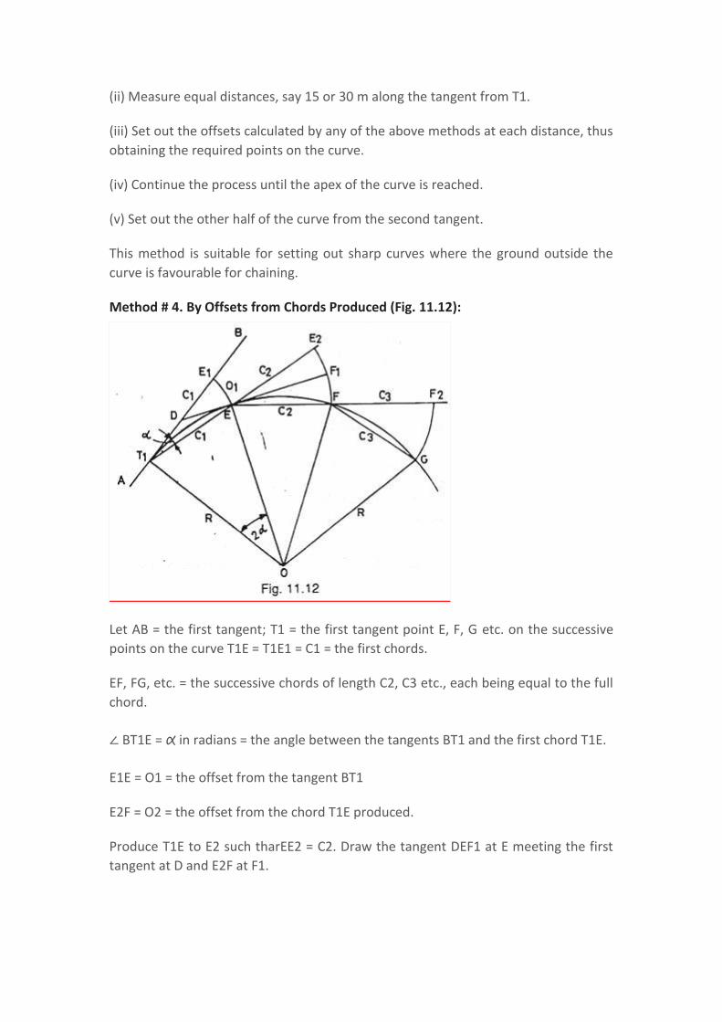
Method # 4. By Offsets from Chords Produced (Fig. 11.12):

Let AB = the first tangent; T1 = the first tangent point E, F, G etc. on the successive

points on the curve T1E = T1E1 = C1 = the first chords.

EF, FG, etc. = the successive chords of length C2, C3 etc., each being equal to the full

chord.

∠ BT1E = α in radians = the angle between the tangents BT1 and the first chord T1E.

E1E = O1 = the offset from the tangent BT1

E2F = O2 = the offset from the chord T1E produced.

Produce T1E to E2 such tharEE2 = C2. Draw the tangent DEF1 at E meeting the first

tangent at D and E2F at F1.

∠BT1E= α in the radians= the angle between the tangents BT1and the first chord

T1E.

E1E=O1= the offset from the tangent BT1

E2F=O2= the offset from the chord T1E produced.

Produce T1E to E2 such that EE2= C2. Draw the tangent DEF1at E meeting the first

tangent at D and E2Fat F1.

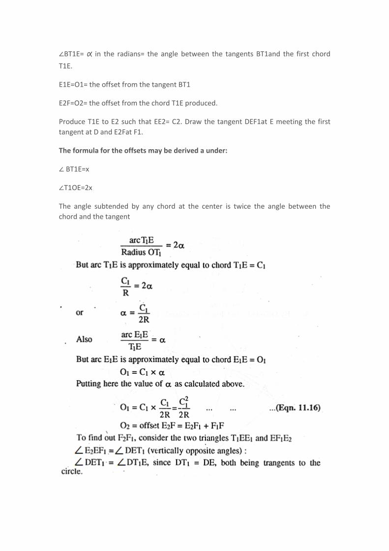
The formula for the offsets may be derived a under:

∠ BT1E=x

∠T1OE=2x

The angle subtended by any chord at the center is twice the angle between the

chord and the tangent

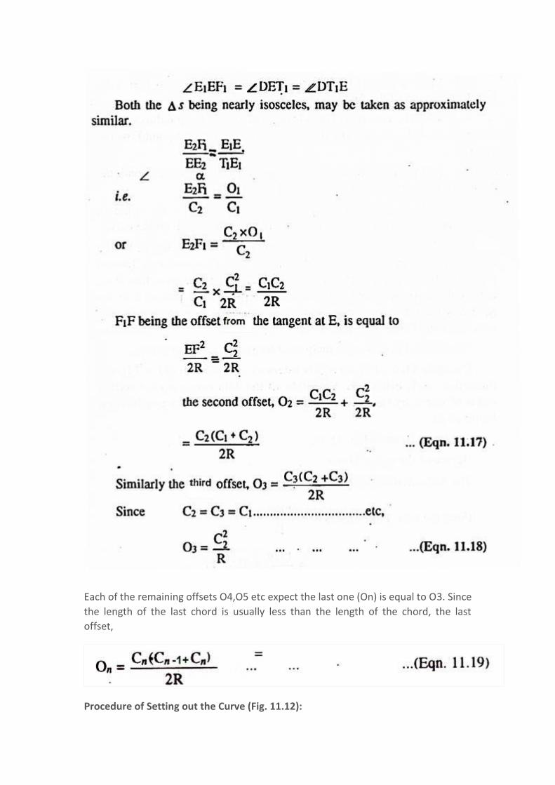
Each of the remaining offsets O4,O5 etc expect the last one (On) is equal to O3. Since

the length of the last chord is usually less than the length of the chord, the last

offset,

Procedure of Setting out the Curve (Fig. 11.12):

(i) Locate the tangent points (T1 and T2) and find out their changes. From these

changes, calculate lengths of first and last sub-chords and find out the offsets by

using the equations 11.16 to 11.19.

(ii) Mark a point E1 along the first tangent T1B such that T1E1 equals the length of

the first sub-chord.

(iii) With the zero end of the chain (or tape) at T1 and radius = T1E1, swing an arc E1E

and cut off E1E = O1, thus fixing the first point E on the curve.

(iv) Pull the chain forward in the direction of T1E produced until the length EE2

becomes equal to the second chord C2.

(v) Hold the zero end of the chain at E. and radius = C2, swing an arc E2F and cut off

E2F = O2, thus fixing the second point F on the curve.

(vi) Continue the process until the end of the curve is reached. The last point fixed in

this way should coincide with the previously located point T2. If not, find the closing

error. If it is large i.e., more than 2 m, the whole curve are moved sideways by an

amount proportional to the square of their distances from the tangent point T1. The

closing error is thus distributed among all the points.

This method is very commonly used for setting out road curves.

Angular Methods for Setting out Curves

The following two methods are the methods of setting out simple circular curves by

angular or instrumental methods: 1. By Rankine’s Tangential Angles. 2. By Two

Theodolites.

Method # 1. Rankine’s Method of Tangential or Deflection Angles: (Fig. 11.14):

In this method, the curve is set out by the tangential angles (also known as

deflection angles) with a theodolite and a chain (or tape). The method is also called

as chain and theodolite method.

The deflection angles are calculated as follows:

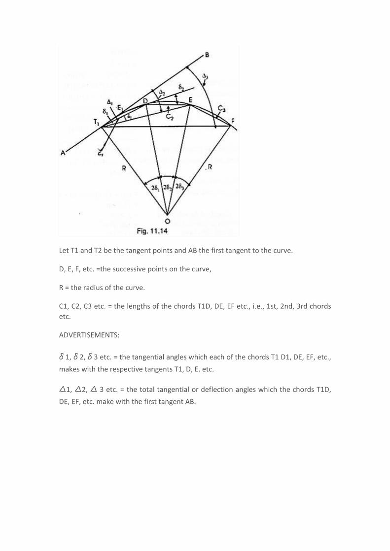
Let T1 and T2 be the tangent points and AB the first tangent to the curve.

D, E, F, etc. =the successive points on the curve,

R = the radius of the curve.

C1, C2, C3 etc. = the lengths of the chords T1D, DE, EF etc., i.e., 1st, 2nd, 3rd chords

etc.

ADVERTISEMENTS:

δ 1, δ 2, δ 3 etc. = the tangential angles which each of the chords T1 D1, DE, EF, etc.,

makes with the respective tangents T1, D, E. etc.

∆1, ∆2, ∆ 3 etc. = the total tangential or deflection angles which the chords T1D,

DE, EF, etc. make with the first tangent AB.

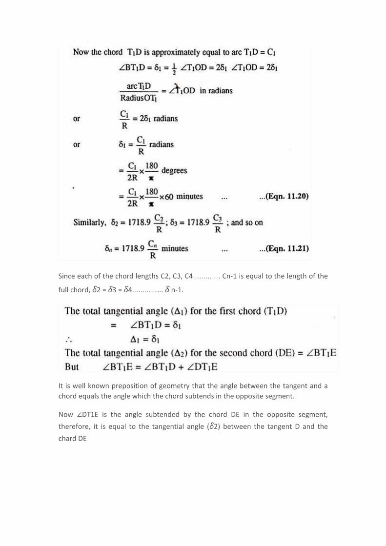
Since each of the chord lengths C2, C3, C4…………. Cn-1 is equal to the length of the

full chord, δ2 = δ3 = δ4…………... δ n-1.

It is well known preposition of geometry that the angle between the tangent and a

chord equals the angle which the chord subtends in the opposite segment.

Now ∠DT1E is the angle subtended by the chord DE in the opposite segment,

therefore, it is equal to the tangential angle (δ2) between the tangent D and the

chard DE

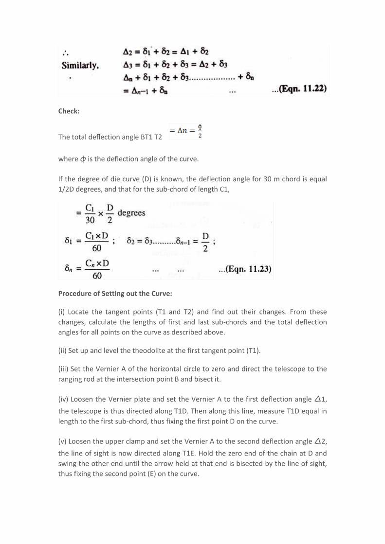
Check:

The total deflection angle BT1 T2

where φ is the deflection angle of the curve.

If the degree of die curve (D) is known, the deflection angle for 30 m chord is equal

1/2D degrees, and that for the sub-chord of length C1,

Procedure of Setting out the Curve:

(i) Locate the tangent points (T1 and T2) and find out their changes. From these

changes, calculate the lengths of first and last sub-chords and the total deflection

angles for all points on the curve as described above.

(ii) Set up and level the theodolite at the first tangent point (T1).

(iii) Set the Vernier A of the horizontal circle to zero and direct the telescope to the

ranging rod at the intersection point B and bisect it.

(iv) Loosen the Vernier plate and set the Vernier A to the first deflection angle Δ1,

the telescope is thus directed along T1D. Then along this line, measure T1D equal in

length to the first sub-chord, thus fixing the first point D on the curve.

(v) Loosen the upper clamp and set the Vernier A to the second deflection angle Δ2,

the line of sight is now directed along T1E. Hold the zero end of the chain at D and

swing the other end until the arrow held at that end is bisected by the line of sight,

thus fixing the second point (E) on the curve.

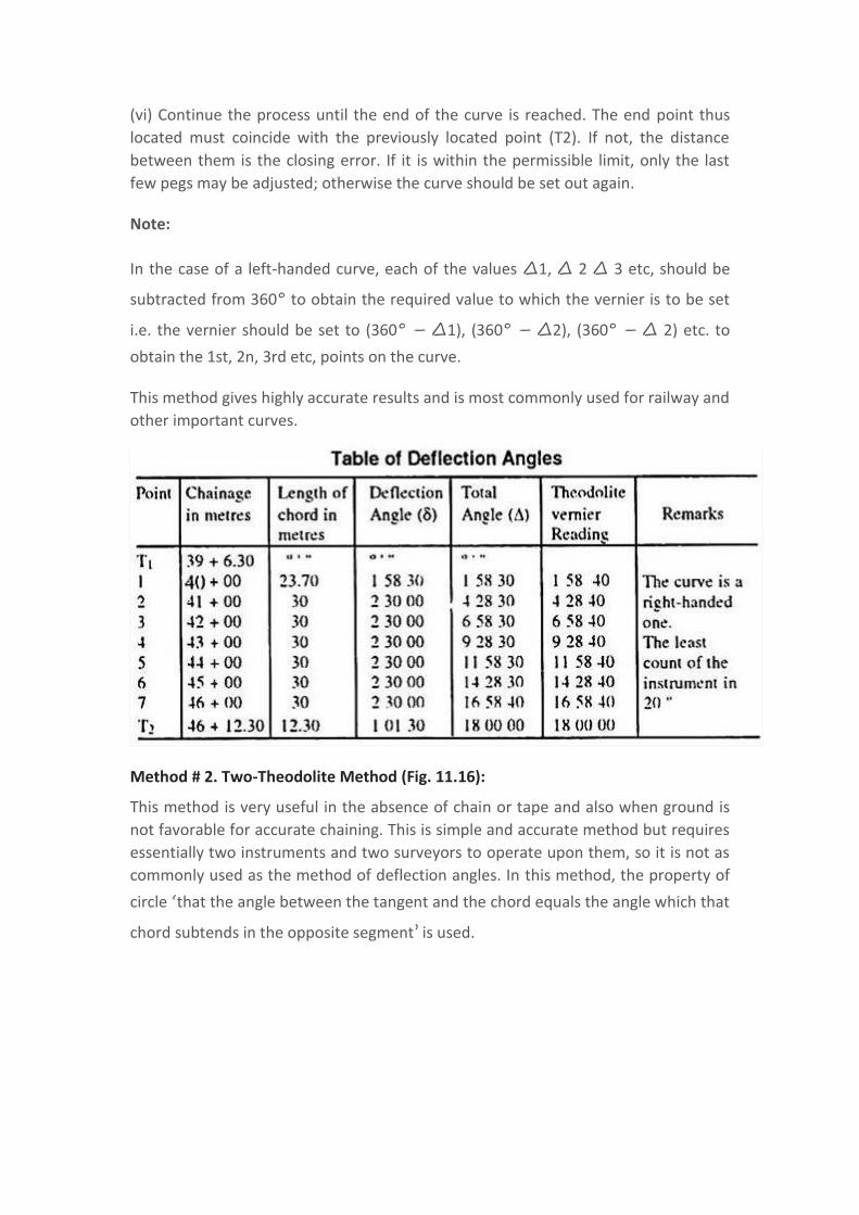
(vi) Continue the process until the end of the curve is reached. The end point thus

located must coincide with the previously located point (T2). If not, the distance

between them is the closing error. If it is within the permissible limit, only the last

few pegs may be adjusted; otherwise the curve should be set out again.

Note:

In the case of a left-handed curve, each of the values Δ1, Δ 2 Δ 3 etc, should be

subtracted from 360° to obtain the required value to which the vernier is to be set

i.e. the vernier should be set to (360° – Δ1), (360° – Δ2), (360° – Δ 2) etc. to

obtain the 1st, 2n, 3rd etc, points on the curve.

This method gives highly accurate results and is most commonly used for railway and

other important curves.

Method # 2. Two-Theodolite Method (Fig. 11.16):

This method is very useful in the absence of chain or tape and also when ground is

not favorable for accurate chaining. This is simple and accurate method but requires

essentially two instruments and two surveyors to operate upon them, so it is not as

commonly used as the method of deflection angles. In this method, the property of

circle ‘that the angle between the tangent and the chord equals the angle which that

chord subtends in the opposite segment’ is used.

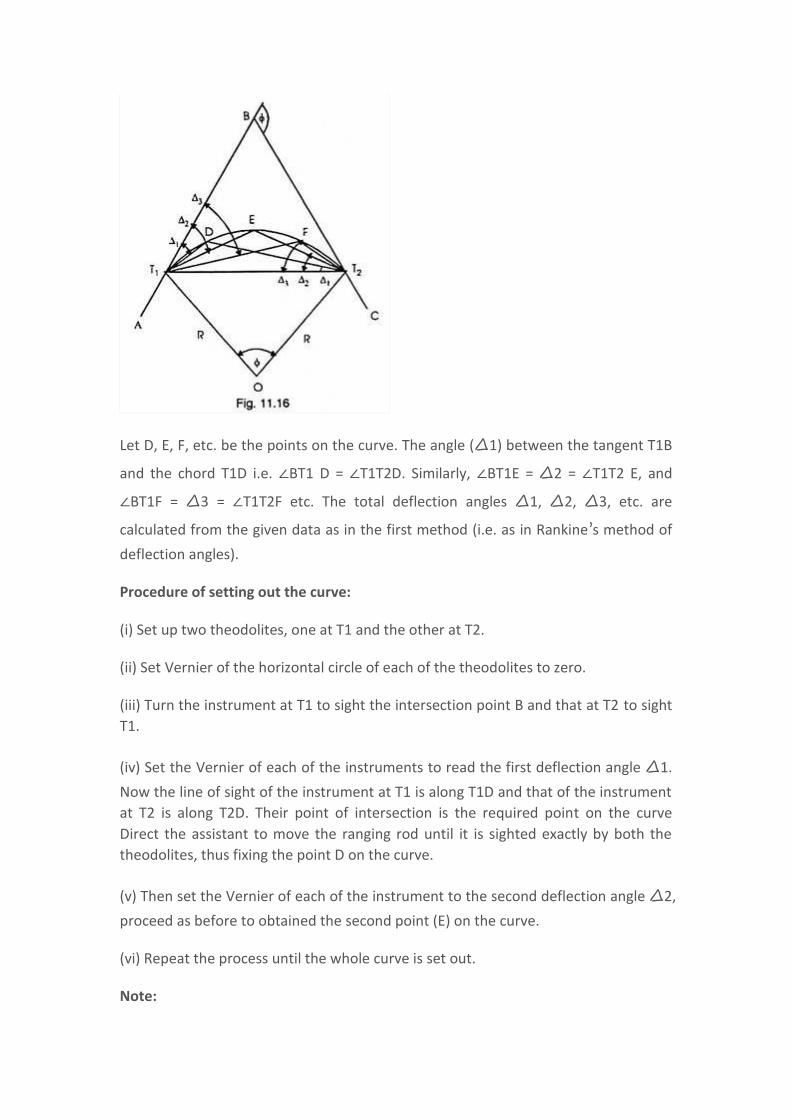
Let D, E, F, etc. be the points on the curve. The angle (Δ1) between the tangent T1B

and the chord T1D i.e. ∠BT1 D = ∠T1T2D. Similarly, ∠BT1E = ∆2 = ∠T1T2 E, and

∠BT1F = ∆3 = ∠T1T2F etc. The total deflection angles ∆1, ∆2, ∆3, etc. are

calculated from the given data as in the first method (i.e. as in Rankine’s method of

deflection angles).

Procedure of setting out the curve:

(i) Set up two theodolites, one at T1 and the other at T2.

(ii) Set Vernier of the horizontal circle of each of the theodolites to zero.

(iii) Turn the instrument at T1 to sight the intersection point B and that at T2 to sight

T1.

(iv) Set the Vernier of each of the instruments to read the first deflection angle Δ1.

Now the line of sight of the instrument at T1 is along T1D and that of the instrument

at T2 is along T2D. Their point of intersection is the required point on the curve

Direct the assistant to move the ranging rod until it is sighted exactly by both the

theodolites, thus fixing the point D on the curve.

(v) Then set the Vernier of each of the instrument to the second deflection angle Δ2,

proceed as before to obtained the second point (E) on the curve.

(vi) Repeat the process until the whole curve is set out.

Note:

It may so happen that the point T1 may not be visible from the point T2. In such a

case, direct the telescope of the instrument at T2 towards B with the Vernier A set to

zero. Now loosen the Vernier plate and set the Vernier A to read an angle of

. The telescope is thus directed along T2 T1. For the first point D on the

curve, set the Vernier A to read . Similarly, for the second point E,

set the Vernier A to , and so on.

Transition Curves:

A non-circular curve of varying radius introduced between a straight and a circular curve for the purpose of giving easy changes of direction of a route is called a transition or easement curve. It is also inserted between two branches of a compound or reverse curve.

Advantages of providing a transition curve at each end of a circular curve:

(i) The transition from the tangent to the circular curve and from the circular curve to the tangent is made gradual.

(ii) It provides satisfactory means of obtaining a gradual increase of super-elevation from zero on the tangent to the required full amount on the main circular curve.

(iii) Danger of derailment, side skidding or overturning of vehicles is eliminated.

(iv) Discomfort to passengers is eliminated.

Conditions to be fulfilled by the transition curve:

(i) It should meet the tangent line as well as the circular curve tangentially.

(ii) The rate of increase of curvature along the transition curve should be the same as that of increase of super-elevation.

(iii) The length of the transition curve should be such that the full super-elevation is attained at the junction with the circular curve.

(iv) Its radius at the junction with the circular curve should be equal to that of circular curve.

There are three types of transition curves in common use:

(1) A cubic parabola,

(2) A cubical spiral, and

(3) A lemniscate, the first two are used on railways and highways both, while the third on highways only.

When the transition curves are introduced at each end of the main circular curve, the combination thus obtained is known as combined or Composite Curve.

Super-Elevation or Cant:

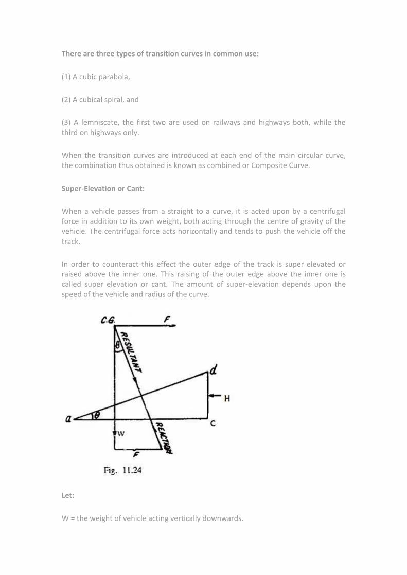
When a vehicle passes from a straight to a curve, it is acted upon by a centrifugal force in addition to its own weight, both acting through the centre of gravity of the vehicle. The centrifugal force acts horizontally and tends to push the vehicle off the track.

In order to counteract this effect the outer edge of the track is super elevated or raised above the inner one. This raising of the outer edge above the inner one is called super elevation or cant. The amount of super-elevation depends upon the speed of the vehicle and radius of the curve.

Let:

W = the weight of vehicle acting vertically downwards.

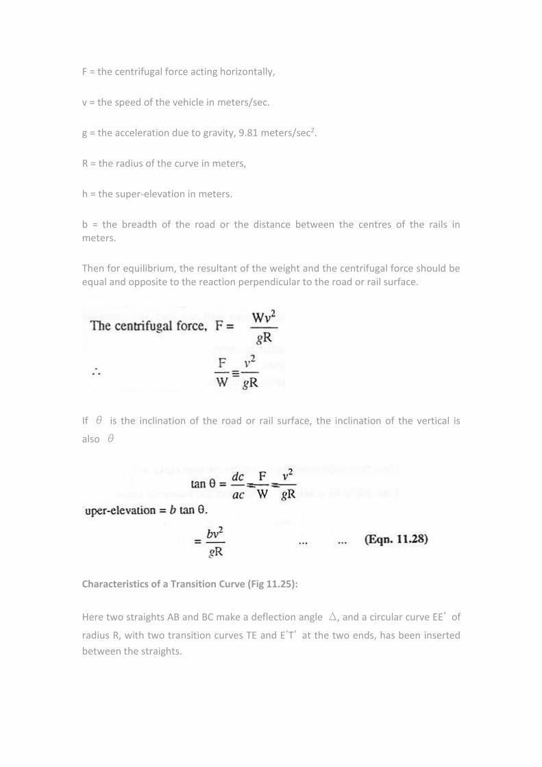
F = the centrifugal force acting horizontally,

v = the speed of the vehicle in meters/sec.

g = the acceleration due to gravity, 9.81 meters/sec2.

R = the radius of the curve in meters,

h = the super-elevation in meters.

b = the breadth of the road or the distance between the centres of the rails in meters.

Then for equilibrium, the resultant of the weight and the centrifugal force should be equal and opposite to the reaction perpendicular to the road or rail surface.

If θ is the inclination of the road or rail surface, the inclination of the vertical is

also θ

Characteristics of a Transition Curve (Fig 11.25):

Here two straights AB and BC make a deflection angle ∆, and a circular curve EE’ of

radius R, with two transition curves TE and E’T’ at the two ends, has been inserted

between the straights.

(i) It is clear from the figure that in order to fit in the transition curves at the ends, a circular imaginary curve (T1F1T2) of slightly greater radius has to be shifted towards the centre as (E1 EF E E1. The distance through which the curve is shifted is known as

shift (S) of the curve, and is equal to , where L is the length of each transition

curve and R is the radius of the desired circular curve (EFE’). The length of shift (T1E1)

and the transition curve (TE) mutually bisect each other.

Fig. 11.25:

(ii) The tangent length for the combined curve

(iii) The spiral angle φ1=

(iv) The central angle for the circular curve:

∠EOE’=∆2ɸ1

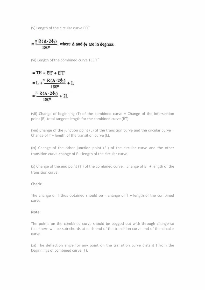
(v) Length of the circular curve EFE’

(vi) Length of the combined curve TEE’T”

(vii) Change of beginning (T) of the combined curve = Change of the intersection point (B)-total tangent length for the combined curve (BT).

(viii) Change of the junction point (E) of the transition curve and the circular curve = Change of T + length of the transition curve (L).

(ix) Change of the other junction point (E’) of the circular curve and the other

transition curve-change of E + length of the circular curve.

(x) Change of the end point (T’) of the combined curve = change of E’ + length of the

transition curve.

Check:

The change of T thus obtained should be = change of T + length of the combined curve.

Note:

The points on the combined curve should be pegged out with through change so that there will be sub-chords at each end of the transition curve and of the circular curve.

(xi) The deflection angle for any point on the transition curve distant I from the beginnings of combined curve (T),

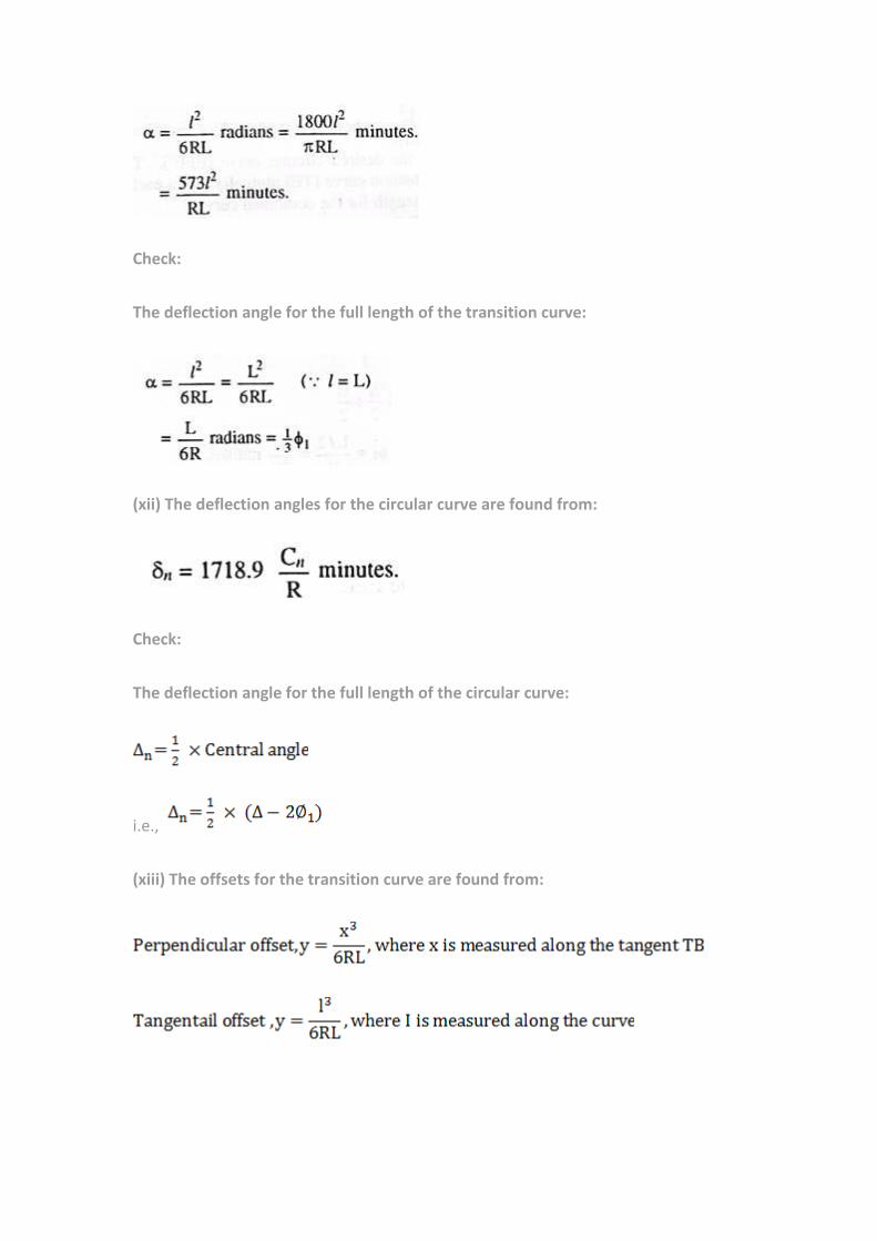
Check:

The deflection angle for the full length of the transition curve:

(xii) The deflection angles for the circular curve are found from:

Check:

The deflection angle for the full length of the circular curve:

i.e.,

(xiii) The offsets for the transition curve are found from:

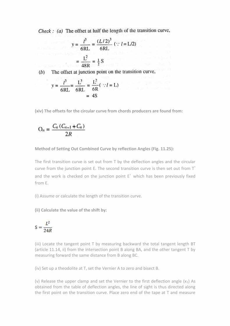
(xiv) The offsets for the circular curve from chords producers are found from:

Method of Setting Out Combined Curve by reflection Angles (Fig. 11.25):

The first transition curve is set out from T by the deflection angles and the circular

curve from the junction point E. The second transition curve is then set out from T’

and the work is checked on the junction point E’ which has been previously fixed

from E.

(i) Assume or calculate the length of the transition curve.

(ii) Calculate the value of the shift by:

(iii) Locate the tangent point T by measuring backward the total tangent length BT (article 11.14, ii) from the intersection point B along BA, and the other tangent T by measuring forward the same distance from B along BC.

(iv) Set up a theodolite at T, set the Vernier A to zero and bisect B.

(v) Release the upper clamp and set the Vernier to the first deflection angle (x1) As obtained from the table of deflection angles, the line of sight is thus directed along the first point on the transition curve. Place zero end of the tape at T and measure

along this line a distance equal to first sub chords, thus locating first point on the transition curve.

(vi) Repeat the process, until the end of the curve E is reached.

Check:

The last deflection angle should be equal to φ1/3, and the perpendicular offset

from the tangent TB for the last point E should be equal to 4S.

Note:

The distance to each of the successive points on the transition curve is measured from T.

(vii) Having laid the transition curve, shift the theodolite to E and set it up and level it accurately.

(viii) Set the Vernier to a reading(360°-2/3 φ1 ) for a right-hand curve (or 2/3 φ1)

for a left-hand curve and lake a back sight on T. Loosen the upper clamp and turn the

telescope clockwise through an angle 2/3 φ1 the telescope is thus directed towards

common tangent at E and the Vernier reads 360°. Transit the telescope, now it

points towards the forward direction of the common tangent at E i.e. towards the tangent for the circular curve.

(ix) Set the Vernier to the first tabulated deflection angle for the circular curve, and locate the first point on the circular curve as already explained in simple curves.

(x) Set out the complete circular curve up to E’ in the usual way

Check:

The last deflection angle should be equal to

(xi) Set out the other transition curve from T as before. The point E’ to be set from T

should be the same as already set out from E.

Method of Setting Out a Combined Curve by Tangential Offsets (Fig. 11.25):

(i) Assume or calculate the length of the transition curve.

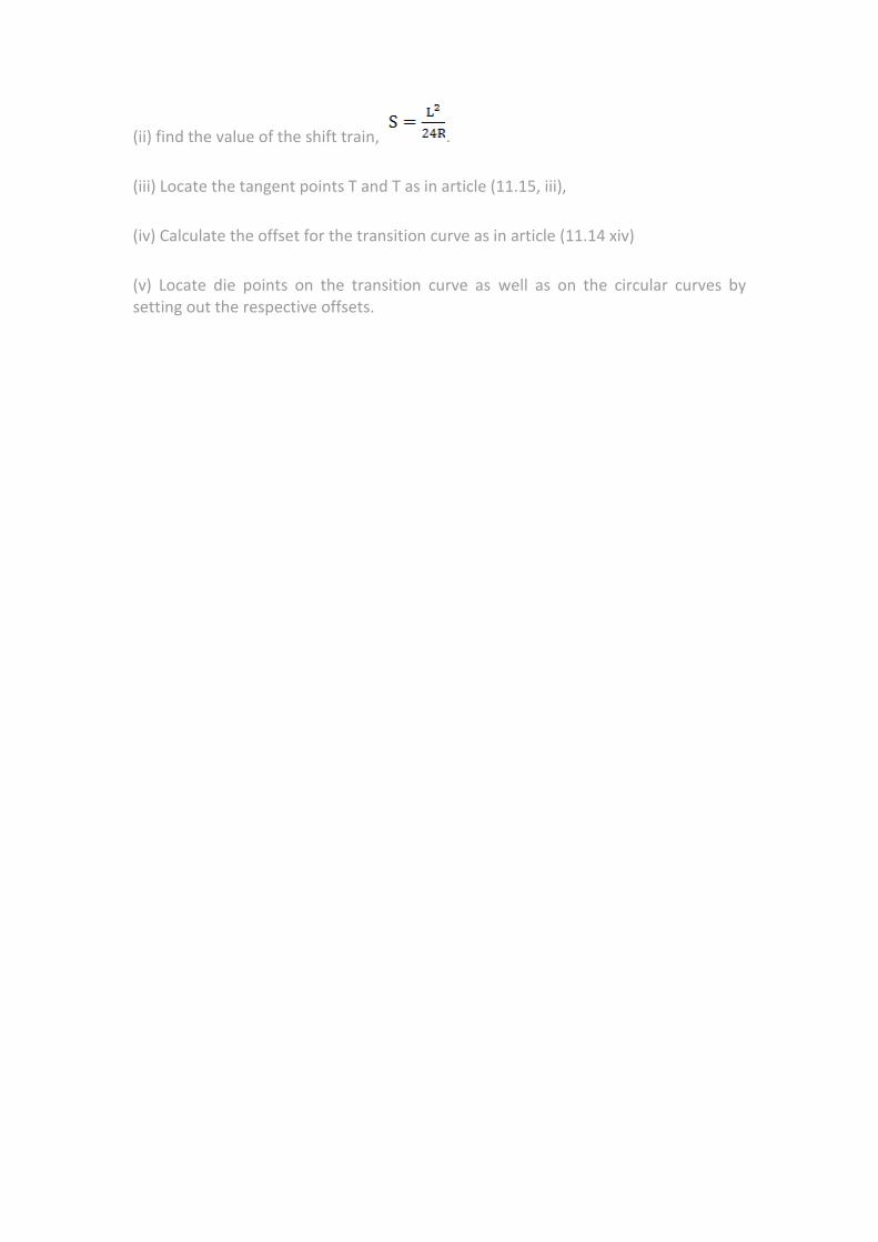
(ii) find the value of the shift train, .

(iii) Locate the tangent points T and T as in article (11.15, iii),

(iv) Calculate the offset for the transition curve as in article (11.14 xiv)

(v) Locate die points on the transition curve as well as on the circular curves by setting out the respective offsets.