Degradation in probability logic: When more information leads to less precise conclusions

Kybernetika

Christian Wallmann; Gernot D. KleiterDegradation in probability logic: When more information leads to less preciseconclusions

Kybernetika, Vol. 50 (2014), No. 2, 268--283

Persistent URL: http://dml.cz/dmlcz/143793

Terms of use:© Institute of Information Theory and Automation AS CR, 2014

Institute of Mathematics of the Academy of Sciences of the Czech Republic provides access to digitizeddocuments strictly for personal use. Each copy of any part of this document must contain theseTerms of use.

This paper has been digitized, optimized for electronic delivery and stampedwith digital signature within the project DML-CZ: The Czech Digital MathematicsLibrary http://project.dml.cz

http://dml.cz/dmlcz/143793

http://project.dml.cz

KYB ERNET IK A — VO LUME 5 0 ( 2 0 1 4 ) , NUMBER 2 , PAGES 2 6 8 – 2 8 3

DEGRADATION IN PROBABILITY LOGIC:WHEN MORE INFORMATION LEADS TO LESS PRECISECONCLUSIONS

Christian Wallmann and Gernot D. Kleiter

Probability logic studies the properties resulting from the probabilistic interpretation of log-ical argument forms. Typical examples are probabilistic Modus Ponens and Modus Tollens.Argument forms with two premises usually lead from precise probabilities of the premises toimprecise or interval probabilities of the conclusion. In the contribution, we study generalizedinference forms having three or more premises. Recently, Gilio has shown that these generalizedforms “degrade” — more premises lead to more imprecise conclusions, i. e., to wider intervals.We distinguish different forms of degradation. We analyse Predictive Inference, Modus Po-nens, Bayes’ Theorem, and Modus Tollens. Special attention is devoted to the case where theconditioning events have zero probabilities. Finally, we discuss the relation of degradation tomonotonicity.

Keywords: probability logic, generalized inference forms, degradation, total evidence, co-herence, probabilistic Modus Tollens

Classification: 03B48, 97K50

1. INTRODUCTION

Consider a knowledge base that contains the observations D1, D2, D3. By the knowledgebase, we evaluate that P (H|D1∧D2) ∈ [0.1, 0.12]. In addition, by the knowledge base, weevaluate that P (H|D1∧D2∧D3) ∈ [0.6, 0.9]. Which one of the two probability intervalsshould we use to update the probability of H? Three properties may be consideredfor this choice: (i) The width of the intervals (the interval [0.1, 0.12] is tighter than[0.6, 0.9]), (ii) the position of the intervals (the positions of [0.1, 0.12] and [0.6, 0.9] arerather different), (iii) the amount of information (D1∧D2 is less specific than D1∧D2∧D3). The principle of total evidence requires to base the updated probability of H onP (H|D1 ∧D2 ∧D3). However, this leads to the more imprecise interval. In probability

DOI: 10.14736/kyb-2014-2-0268

http://doi.org/10.14736/kyb-2014-2-0268

Degradation in probability logic 269

logic1 conflicts between the amount of evidence and the precision of the conclusions arequite typical [4]. Especially in inferences that generalize common inference forms, likegeneralized Modus Ponens or Modus Tollens, more specific information leads to moreimprecise probabilities of the conclusions. The fact that the width of the interval of theconclusion increases as the number of premises increases has been called “degradationin probability logic”. In the extreme case, the probability of the conclusion may benoninformative, i. e., may attain any value between zero and one [4, 7, 12, 13].

Probability logic studies the properties resulting from the probabilistic interpretationof logical argument forms. It determines the set of all coherent probability values ofthe conclusion if a coherent probability assessment on the premises is given. This setis according to de Finetti’s Fundamental Theorem [2, 9] an interval or a point value.The probability of a conditional P (A ⇒ B) is represented by the conditional probabilityP (B|A). Consider, for example, Modus Ponens. Its logical form infers from the premises{A,A ⇒ B} the conclusion B. Accordingly, the probabilistic version of Modus Ponensinfers from the premises {P (A) = α, P (B|A) = β} the conclusion P (B) ∈ [αβ, αβ + 1−α]. Generalized probabilistic Modus Ponens determines the interval P (H) ∈ [δ′, δ′′] ifthe premises {P (E1) = α1, . . . , P (En) = αn, P (H|

∧ni=1 Ei) = β} are given (see Section

2.5 below).For a generalized inference form we denote by In the interval for the conclusion if

n premises are given. Let |Ii| be the width of the interval Ii. A generalized inferenceform degrades if and only if for all i, j ∈ N: If i < j, then |Ii| ≤ |Ij |. A differentposition of the interval, which is based on more premises, may compensate for a widerinterval (compare the intervals [0.6, 0.9] and [0.1, 0.12] in the introductory example). Tostudy degradation in more detail, we therefore distinguish two forms of degradation. Ageneralized inference form strongly degrades if and only if for all i, j ∈ N: If i < j, thenIi ⊆ Ij (i. e., the former interval is included in the latter). A generalized inference formweakly degrades if and only if it degrades and if for some k, l ∈ N Ik 6⊆ Il and Il 6⊆ Ik

(i. e., the latter interval is wider but does not include the former). In general, however,the preference of intervals with different width and intervals with different positions isa difficult task and both forms of degradation are problematic for the application ofprobability logic to generalized inference forms.

In this contribution, we analyse generalizations of Modus Ponens, Predictive Infer-ence, Conjunction, Bayes’ Theorem, and Modus Tollens for the different kinds of degra-dation. It is common to all of the inference forms considered in the present paper —with the exception of Modus Tollens — that a certain form of ultimate degradation isobserved. If the number of premises is sufficiently high, then the interval of the conclu-sion is the unit interval [0, 1]. The reason is that the lower bound of the conjunctionof n events P (

∧ni=1 Ei) quickly becomes zero if the number of conjuncts n increases.

The fact that the lower bound of the conjunction is often zero has the consequence thatthe conditioning event of many conditional events has zero probability. We thereforepay special attention to this case. In particular, we study the generalization of Bayes’Theorem when the prior probability of the hypothesis is zero or when the data has zero

1If probabilities of conditionals P (A ⇒ B) are represented by conditional probabilities P (B|A), thenone usually speaks of conditional probability logic. However, in the remainder of the paper, we use theexpression ‘probability logic’ instead of ‘conditional probability logic’.

270 C. WALLMANN AND G.D. KLEITER

probability. The case when the conditioning event has zero probability can be treatedin the coherence approach of de Finetti [1, 2]. Furthermore, we prove the result forthe generalized Modus Tollens stated in [7, 12, 13]. Finally, we discuss the relation ofdegradation to monotonicity and its significance for uncertain reasoning. In particular,we show that probability logic is weak for decision making and that it should thereforebe supplemented by additional principles.

2. DEGRADATION OF INFERENCES IN PROBABILITY LOGIC

2.1. Terminology

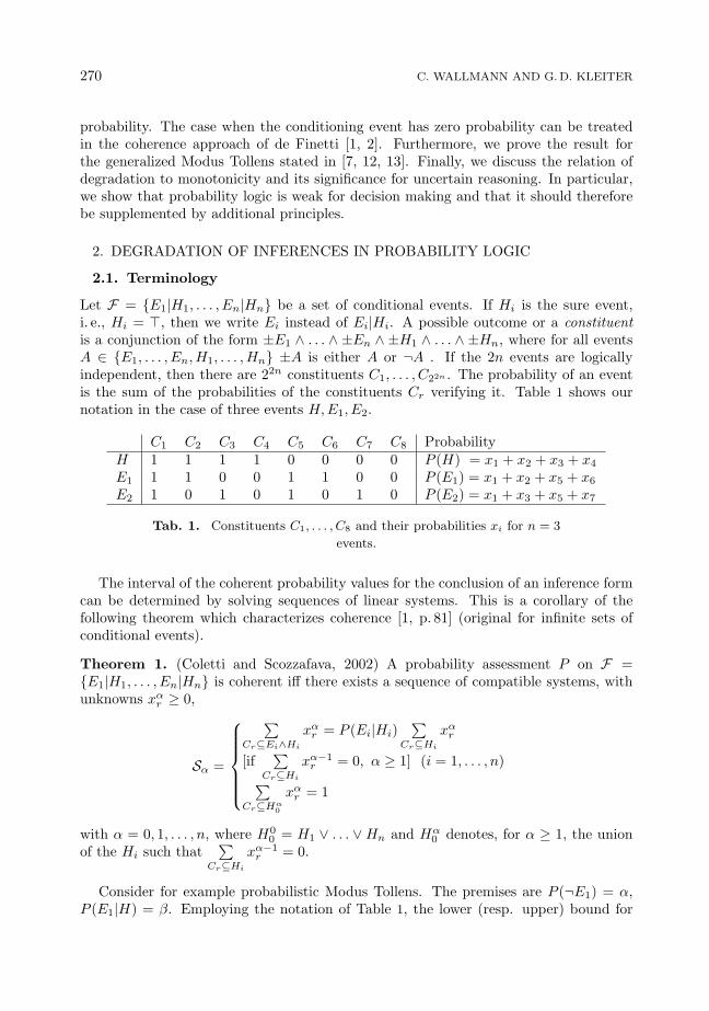
Let F = {E1|H1, . . . , En|Hn} be a set of conditional events. If Hi is the sure event,i. e., Hi = >, then we write Ei instead of Ei|Hi. A possible outcome or a constituentis a conjunction of the form ±E1 ∧ . . . ∧ ±En ∧ ±H1 ∧ . . . ∧ ±Hn, where for all eventsA ∈ {E1, . . . , En,H1, . . . ,Hn} ±A is either A or ¬A . If the 2n events are logicallyindependent, then there are 22n constituents C1, . . . , C22n . The probability of an eventis the sum of the probabilities of the constituents Cr verifying it. Table 1 shows ournotation in the case of three events H,E1, E2.

C1 C2 C3 C4 C5 C6 C7 C8 ProbabilityH 1 1 1 1 0 0 0 0 P (H) = x1 + x2 + x3 + x4

E1 1 1 0 0 1 1 0 0 P (E1) = x1 + x2 + x5 + x6

E2 1 0 1 0 1 0 1 0 P (E2) = x1 + x3 + x5 + x7

Tab. 1. Constituents C1, . . . , C8 and their probabilities xi for n = 3

events.

The interval of the coherent probability values for the conclusion of an inference formcan be determined by solving sequences of linear systems. This is a corollary of thefollowing theorem which characterizes coherence [1, p. 81] (original for infinite sets ofconditional events).

Theorem 1. (Coletti and Scozzafava, 2002) A probability assessment P on F ={E1|H1, . . . , En|Hn} is coherent iff there exists a sequence of compatible systems, withunknowns xα

r ≥ 0,

Sα =

∑Cr⊆Ei∧Hi

xαr = P (Ei|Hi)

∑Cr⊆Hi

xαr

[if∑

Cr⊆Hi

xα−1r = 0, α ≥ 1] (i = 1, . . . , n)∑

Cr⊆Hα0

xαr = 1

with α = 0, 1, . . . , n, where H00 = H1 ∨ . . . ∨Hn and Hα

0 denotes, for α ≥ 1, the unionof the Hi such that

∑Cr⊆Hi

xα−1r = 0.

Consider for example probabilistic Modus Tollens. The premises are P (¬E1) = α,P (E1|H) = β. Employing the notation of Table 1, the lower (resp. upper) bound for


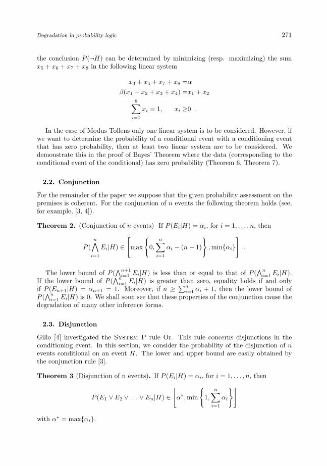
the conclusion P (¬H) can be determined by minimizing (resp. maximizing) the sumx5 + x6 + x7 + x8 in the following linear system

x3 + x4 + x7 + x8 =α

β(x1 + x2 + x3 + x4) =x1 + x2

8∑i=1

xi = 1, xi ≥0 .

In the case of Modus Tollens only one linear system is to be considered. However, ifwe want to determine the probability of a conditional event with a conditioning eventthat has zero probability, then at least two linear system are to be considered. Wedemonstrate this in the proof of Bayes’ Theorem where the data (corresponding to theconditional event of the conditional) has zero probability (Theorem 6, Theorem 7).

2.2. Conjunction

For the remainder of the paper we suppose that the given probability assessment on thepremises is coherent. For the conjunction of n events the following theorem holds (see,for example, [3, 4]).

Theorem 2. (Conjunction of n events) If P (Ei|H) = αi, for i = 1, . . . , n, then

P (n∧

i=1

Ei|H) ∈

[max

{0,

n∑i=1

αi − (n− 1)

},min{αi}

].

The lower bound of P (∧n+1

i=1 Ei|H) is less than or equal to that of P (∧n

i=1 Ei|H).If the lower bound of P (

∧ni=1 Ei|H) is greater than zero, equality holds if and only

if P (En+1|H) = αn+1 = 1. Moreover, if n ≥∑n

i=1 αi + 1, then the lower bound ofP (

∧ni=1 Ei|H) is 0. We shall soon see that these properties of the conjunction cause the

degradation of many other inference forms.

2.3. Disjunction

Gilio [4] investigated the System P rule Or. This rule concerns disjunctions in theconditioning event. In this section, we consider the probability of the disjunction of nevents conditional on an event H. The lower and upper bound are easily obtained bythe conjunction rule [3].

Theorem 3 (Disjunction of n events). If P (Ei|H) = αi, for i = 1, . . . , n, then

P (E1 ∨ E2 ∨ . . . ∨ En|H) ∈

[α∗,min

{1,

n∑i=1

αi

}]

with α∗ = max{αi}.


P r o o f . We note that∨n

i=1 Ei is equivalent to ¬∧n

i=1 ¬Ei and, accordingly, P (∨n

i=1 Ei|H)= 1−P (

∧ni=1 ¬Ei|H). We denote P (

∨ni=1 Ei|H) by α. As P (¬Ei|H) = 1−αi, we know

the probability of the negation of each of the events and we can apply the conjunctiontheorem to the n negated events to obtain the disjunction. We have

1− α = P (n∧

i=1

¬Ei|H) ∈

[max

{0,

n∑i=1

(1− αi)− (n− 1)

},min{1− αi}

]. (2.1)

Using P (∨n

i=1 Ei|H) = 1− P (∧n

i=1 ¬Ei|H) and (2.1), we obtain

α ∈

[α∗,min

{1,

n∑i=1

αi

}]. (2.2)

�

An upper bound of the disjunction of n events, that is different from 1, is gettingwider, if αn+1 6= 0.

2.4. Predictive Inference

Predictive Inference is one of the key inference rules in Bayesian statistics. It determinesthe predictive probability P (H|E1 ∧ . . . ∧ Er ∧ ¬Er+1 ∧ . . . ∧ ¬En) of H after havingobserved r successes and n− r failures in the set {Ei}n

i=1. It is of main importance if His regarded exchangeable with the other events. If at least one of the events {Ei}n

i=1 didnot occur, i. e., r < n, then the interval obtained for the predictive probability is the unitinterval [12]. As observed in [12], the case where all previous trials were successes, i. e.,r = n, is a special case of the System P rule Cautious Monotonicity. Consequently, thefollowing theorem is a corollary of the result for Cautious Monotonicity stated in [4].

Theorem 4. (Predictive probability) If P (H) = β and P (Ei) = αi, for i = 1, . . . , n,then P (H|E1 ∧ . . . ∧ En) ∈ [γ′, γ′′], with

γ′ =

max{

0,β+

Pni=1 αi−nPn

i=1 αi−(n−1)

}if

∑ni=1 αi − (n− 1) > 0

0 if∑n

i=1 αi − (n− 1) ≤ 0

γ′′ =

min{

1, βPni=1 αi−(n−1)

}if

∑ni=1 αi − (n− 1) > 0

1 if∑n

i=1 αi − (n− 1) ≤ 0.

We compare this result with the result for the case where the premise P (En+1) = αn+1

is added and the conclusion is H|E1 ∧ . . . ∧ En ∧ En+1. Observe that in both cases thesame event H is predicted. Theorem 4 shows that the upper bound of the conclusionincreases and that its lower bound decreases. Thus, the interval gets wider if a new eventis added and the old interval is a subset of the new interval. Consequently, in the caseof predictive inference we have a strong degradation. Furthermore, if n ≥

∑ni=1 αi + 1,

then P (H|E1 ∧ . . .∧En) ∈ [0, 1]. The property that the lower bound of the conjunctiondecreases is the reason for both, the strong degradation of Predictive Inference and forobtaining the unit interval if n is large.


2.5. Modus Ponens

Modus Ponens is a special case of the System P rule Cut. The following theorem is acorollary of Gilio’s result for the generalization of the Cut rule [4].

Theorem 5. (Modus Ponens) If P (Ei) = αi, for i = 1, . . . , n, and P (H|∧n

i=1 Ei) = β,then

P (H) ∈ [βσn , βσn + 1− σn],

with σn = max

{0,

n∑i=1

αi − (n− 1)

}.

We compare this result with the result where P (En+1) = αn+1 is added to thepremises and P (H|

∧ni=1 Ei) = β is replaced by P (H|

∧n+1i=1 Ei) = γ. If γ = β, then

Modus Ponens strongly degrades. However, even if β 6= γ, the width of the interval forP (H) normally increases. This follows from the facts that its width is 1− σn and thatσn normally decreases. Consequently, that the lower bound of the conjunction decreasescauses the degradation of Modus Ponens. However, since β is replaced by γ 6= β, theposition of the interval for P (H) may change. Therefore, in the case of Modus Ponensa weak degradation is observed.

Example 1. Consider the premise sets T and T ′ such thatT = {P (E1) = 0.9, P (E2) = 0.8, P (E3) = 0.95, P (H|E1 ∧ E2 ∧ E3) = 0.8} andT ′ ={P (E1) = 0.9, P (E2) = 0.8, P (E3) = 0.95, P (E4) = 0.8, P (H|E1∧E2∧E3∧E4) =0.1}.From T it follows that P (H) ∈ [0.52, 0.87], whereas from T ′ it follows that P (H) ∈[0.045, 0.595].

The width of the interval 1− σn depends on the lower bound of the conjunction σn.Since this lower bound is zero if n ≥

∑ni=1 αi + 1, the interval for P (H) is the unit

interval if the number of premises is sufficiently high.

2.6. Bayes’ theorem

Suppose that the prior probability of a certain hypothesis P (H) = δ, the likelihoodsof the data given both, the hypothesis H, P (D|H) = β, and the alternative hypoth-esis ¬H, P (D|¬H) = γ, are given. The posterior probability of the hypothesis Hgiven the data D is obtained by Bayes’ Theorem P (H|D) = βδ

βδ+γ(1−δ) . The premisesof generalized Bayes’ Theorem are P (H) = δ, P (E1|H) = β1, . . . , P (En|H) = βn,P (E1|¬H) = γ1, . . . , P (En|¬H) = γn. In inferential statistics it is often assumed thatthe Ei’s are independent and identically distributed. To be as general as possible,we do neither require conditional independence of the Ei’s given H nor do we requirethat P (Ei|H) = P (Ej |H) for i 6= j. The conclusion of generalized Bayes’ Theorem is


P (H|E1 ∧ . . . ∧ En). Observe that if P (E1 ∧ . . . ∧ En) > 0, then

P (H|E1 ∧ . . . ∧ En) =P (H ∧ E1 ∧ . . . ∧ En)

P (E1 ∧ . . . ∧ En)

=P (H)P (E1 ∧ . . . ∧ En|H)

P (H)P (E1 ∧ . . . ∧ En|H) + P (¬H)P (E1 ∧ . . . ∧ En|¬H).

(2.3)

To prove the result for the generalization of Bayes’ Theorem (Theorem 6 and Theo-rem 7) we consequently treat two cases for the probability of the data P (E1 ∧ . . .∧En):(i) P (E1 ∧ . . .∧En) > 0 and (ii) P (E1 ∧ . . .∧En) = 0. In case (ii) it is relevant whetherthe prior probability P (H) is zero, one, or different from both values. To handle case(ii) properly we make use of Theorem 1. The special case n = 1 has been investigatedin detail by Coletti and Scozzafava [1, Chapter 16]. The proofs of the next two resultsare obtained by analogous considerations; hence, we omit the first one.

Theorem 6. (Bayes’ Theorem, lower bound) Suppose that P (H) = δ and that for alli = 1, . . . , n, P (Ei|H) = βi and P (Ei|¬H) = γi. Then:

• If δ(∑n

i=1 βi − (n− 1)) > 0, then

P (H|E1 ∧ . . . ∧ En) ≥δ(

∑ni=1 βi − (n− 1))

δ(∑n

i=1 βi − (n− 1)) + (1− δ) min{γi}.

• If δ(∑n

i=1 βi − (n− 1)) ≤ 0, then P (H|E1 ∧ . . . ∧ En) ≥ 0.

Theorem 7. (Bayes’ Theorem, upper bound) Suppose that P (H) = δ and that for alli = 1, . . . , n, P (Ei|H) = βi and P (Ei|¬H) = γi. Then:

• If (1− δ)(∑n

i=1 γi − (n− 1)) > 0, then

P (H|E1 ∧ . . . ∧ En) ≤ δ min{βi}δ min{βi}+ (1− δ)(

∑ni=1 γi − (n− 1))

.

• If (1− δ)(∑n

i=1 γi − (n− 1)) ≤ 0, then P (H|E1 ∧ . . . ∧ En) ≤ 1.

P r o o f . We distinguish two cases.(I) If (1− δ)(

∑ni=1 γi − (n− 1)) > 0, then P (E1 ∧ . . . ∧En) > 0. The result is obtained

by application of the Conjunction Theorem (Theorem 2) to (2.3).(II) If (1− δ)(

∑ni=1 γi− (n− 1)) ≤ 0, we distinguish two cases (i) δ min{βi} > 0 and (ii)

δ min{βi} = 0.In case (i) the upper bound 1 is obtained by setting P (H∧E1∧. . .∧En) to δ min{βi} > 0and P (¬H ∧ E1 ∧ . . . ∧ En) to its minimum 0.In case (ii) we obtain the upper bound by setting the probability of the data P (E1 ∧. . . ∧ En) to 0. We treat the case n = 2. The proof generalizes to the case n > 2


straightforwardly. We build the sequence of linear systems Sα (Theorem 1). To improvereadability we write xi instead of x0

i , yi instead of x1i , and zi instead of x2

i .Using the notation of Table 1, the first linear system S0 is given by

x1 + x5 = 0P (H|E1 ∧ E2)(x1 + x5) = x1

x1 + x2 + x3 + x4 = δ

x1 + x2 = β1(x1 + x2 + x3 + x4), x1 + x3 = β2(x1 + x2 + x3 + x4)x5 + x6 = γ1(x5 + x6 + x7 + x8), x5 + x7 = γ2(x5 + x6 + x7 + x8)

x1 + x2 + x3 + x4 + x5 + x6 + x7 + x8 = 1, xi ≥ 0 .

As unique solution of S0 we obtain x1 = x5 = 0, x2 = β1δ, x3 = β2δ, x4 = δ −(β1 + β2)δ, x6 = γ1(1 − δ), x7 = γ2(1 − δ), x8 = (1 − δ) − (γ1 + γ2)(1 − δ). Sinceδ min{β1, β2} = 0, it holds that x4 = δ(1−β1−β2) = δ(1−max{β1, β2}) ≥ 0, and sinceby assumption γ1 + γ2 ≤ 1, it is x8 ≥ 0, so that the solution is admissible.If 0 < P (H) = δ < 1, then H1

0 = E1 ∧ E2. The system S1 is consequently given by

P (H|E1 ∧ E2)(y1 + y5) = y1

y1 + y5 = 1, yi ≥0 .

So that P (H|E1 ∧ E2) = y1y1+y5

can attain any value in [0, 1].

If P (H) = δ = 0 (the case P (H) = 1 is treated in the same way), then x1 = x2 = x3 =x4 = x5 = 0 and consequently H1

0 = H ∨ (E1 ∧ E2). In the system S ′1 all constraintsthat concern conditional events with conditioning event H remain.

P (H|E1 ∧ E2)(y1 + y5) =y1

y1 + y2 = β1(y1 + y2 + y3 + y4), y1 + y3 =β2(y1 + y2 + y3 + y4)y1 + y2 + y3 + y4 + y5 =1, yi ≥ 0 .

We solve S ′1 in such a way that P (H) > 0 and P (E1 ∧E2) = 0. The unique solutionin this case is y2 = β1, y3 = β2, y4 = 1− (β1 + β2). Then H2

0 = E1 ∧ E2 and the thirdsystem S ′2 is

P (H|E1 ∧ E2)(z1 + z5) =z1

z1 + z5 = 1, zi ≥0 .

So that P (H|E1 ∧ E2) = z1z1+z5

can attain any value in [0, 1].In both cases, 0 < P (H) < 1 and P (H) = 0, we have constructed a sequence ofcompatible systems (Sα), with unknowns (xα

i ), i = 1, . . . , 8, α = 0, 1, 2, such thatP (H|E1 ∧ E2) ∈ [0, 1]. According to Theorem 1 P (H|E1 ∧ E2) can coherently attainany value in [0, 1]. �

In the present paper the non uniquely determined probabilities result from the factthat no knowledge about the association (conditional independence or kind of depen-dence) of the data given the hypothesis is presumed. For a slightly more general ap-proach to iterated conditioning in Bayes’ Theorem and the accordingly also non uniquelydetermined probabilities see [5].


Bayes’ Theorem does not degrade. First of all, Bayes’ Theorem does not degradestrongly. The lower bound is not monotonically decreasing, because it depends on theminimum of the set {γi}. If for a given n the premises P (En+1|¬H) = γn+1 < min{γi}and P (En+1|H) = βn+1 are added, the lower bound may increase. Similar considerationsshow that the upper bound is not monotonically increasing. As a consequence, intervalswith rather different positions may result.

Example 2. Suppose that P (H) = 0.1, P (E1|H) = 0.9, P (E2|H) = 0.8, P (E3|H) =0.4, P (E1|¬H) = 0.9999, P (E2|¬H) = 0.9999, P (E3|¬H) = 0.001. Then P (H|E1 ∧E2) ∈ [0.072, 0.081], but P (H|E1 ∧ E2 ∧ E3) = [0.917, 0.982] .2

In Bayes’ Theorem even no weak degradation is observed. In general, the probabilityinterval of the conclusion need not get wider as the number of premises increases.

Example 3. Suppose that P (H) = 0.9, P (E1|H) = 0.99, P (E2|H) = 0.99, P (E3|H) =0.98, P (E1|¬H) = 0.9999, P (E2|¬H) = 0.9999, P (E3|¬H) = 0.001. Then P (H|E1 ∧E2) ∈ [0.898176, 0.89911] , but P (H|E1 ∧ E2 ∧ E3) ∈ [0.999884, 0.999909], so that thewidth of the first interval is 0.000934 and that of the second interval is 0.000025 .3

This does by no means imply that additional information makes the situation nec-essarily better. In many cases the interval does get wider if the number of premisesincreases. If, for instance, identical probabilities βi = β and γi = γ for i = 1, . . . , n,are assumed, then Bayes’ Theorem strongly degrades. This case is of main importancebecause it is implied by the assumption of conditional exchangeability. Moreover, The-orem 6 and Theorem 7 show that even in the case of Bayes’ Theorem one ends up withthe unit interval. If n ≥ max {

∑ni=1 βi + 1,

∑ni=1 γi + 1}, then

∑ni=1 βi − (n − 1) ≤ 0

and∑n

i=1 γi − (n− 1) ≤ 0, so that the interval [0, 1] is obtained.We therefore claim that Bayesian updating, i. e., the new probability of a hypothesis

H after observing E1, E2, . . . , En should be measured by P (H|E1 ∧ E2 ∧ . . . ∧ En), isaccurate only under very restricted assumptions. One such assumption is conditionalindependence, leading to a point probability of the likelihood P (E1 ∧ . . . ∧ En|H).

2.7. Modus Tollens

The following holds for the probabilistic Modus Tollens of two events as we show below(Theorem 8). If P (¬E1) = α1 and P (E1|H) = β, then P (¬H) ∈ [δ′, 1], where

δ′ = max{

1− α1

1− β, 1− 1− α1

β

}. (2.4)

Wagner [11] has shown the result for the lower bound. However, Wagner’s upperbound is different from 1. The reason for this is that Wagner defined the conditionalprobability P (E1|H) by the fraction P (E1∧H)

P (H) . If P (¬H) = 1, then P (H) = 0 andP (E1|H) would consequently be undefined. As already pointed out, in the coherenceapproach conditionalizing on events with zero probability is possible, so that the “cor-rect” upper bound P (¬H) = 1 is obtained.

2All values are rounded.3All values are rounded.


The result for the generalized Modus Tollens has been presented without proof in[7, 12].

Theorem 8. (Modus Tollens) If P (¬Ei) = αi, for i = 1, 2, . . . , n, and if P (E1 ∧ E2 ∧. . . ∧ En|H) = β, then P (¬H) ∈ [δ′, 1], with

δ′ =

1− 1−α∗

β if α∗ + β > 1,

1−Pn

i=1 αi

1−β if∑n

i=1 αi + β < 1,

0 if∑n

i=1 αi + β ≥ 1 and α∗ + β ≤ 1,

where α∗ = max{αi}.

P r o o f . First, we treat the case n = 1. Then we use this result and the conjunctionrule (Theorem 2) to prove the general case n > 1.

One event. If n = 1, we employ the following notation

C1 C2 C3 C4 ProbabilityH 1 1 0 0 P (H) = x1 + x2

E1 1 0 1 0 P (E1) = x1 + x3 = 1− α1

and obtain the linear system

β(x1 + x2) = x1 (2.5)x2 + x4 = α1 (2.6)

x1 + x2 + x3 + x4 = 1, xi ≥ 0 .

To maximize (resp. minimize) P (¬H), we minimize (resp. maximize)

P (H) = x1 + x2 .

Manipulation of (2.5) shows that if β > 0, then

P (H) =x1

β. (2.7)

If β = 0, then the solvability of the above linear system requires that P (H) = x2 ∈ [0, α1]and therefore P (¬H) ∈ [1− α1, 1].Because of (2.7), to maximize (minimize) P (H) in case of β > 0, we maximize (minimize)x1 = P (H ∧ E1).

Upper bound of P (¬H). The minimum x1 = 0 is obtained by setting x4 = α1.

Lower bound of P (¬H). For the maximum of x1 observe that x1 ≤ 1−α1. Furthermore,since P (H ∧ E1) ≤ P (E1|H), we have x1 ≤ β. Therefore, x1 ≤ min{1 − α1, β} and wedistinguish two cases: (I) 1− α1 ≤ β and (II) 1− α1 > β.


In case (I), we set x1 to its maximum 1−α1. By (2.7) we obtain P (H) = 1−α1β , so that

the minimum of P (¬H) is 1− 1−α1β . It is straightforward to establish that the solution

x1 = 1− α1 is admissible.In case (II), we cannot set x1 to its maximum β. Otherwise, we have x1 + x3 + x4 =β + α1 > 1. We employ that by (2.5), it is x1 = x2β

1−β . Hence, x1 is maximized if x2

is maximized. This is the case if x2 = α1 (and hence x4 = 0), so that x1 = α1β1−β .

Consequently

x3 = P (¬H) = 1− (x1 + x2) = 1−(α1)β1−β

β= 1− α1

1− β.

n events. Employing the case n = 1, writing E :=∧n

i=1 Ei, we obtain that if P (¬E) = αand if P (E|H) = β, then P (¬H) ∈ [δ′, 1], where

δ′ =

1− 1−α

β if α + β > 1,

1− α1−β if α + β < 1,

0 if α + β = 1 .

(2.8)

Applying the disjunction rule (Theorem 3) to P (¬Ei) = αi, yields for α = P (¬E) =P (

∨ni=1 ¬Ei)

α ∈

[α∗,min

{1,

n∑i=1

αi

}]. (2.9)

Applying (2.9) to (2.8) and distinguishing cases proves the result:

Case 1: If α∗+β > 1, then α+β > 1. According to (2.8), since 1− 1−αβ is monotonically

increasing with α, the minimum is 1− 1−α∗

β .Case 2: If α∗ + β ≥ 1, we distinguish two cases.(2.1): If

∑ni=1 αi + β < 1, then since α ≤

∑ni=1 αi, we have α + β < 1. Since 1− α

1−β is

monotonically decreasing in α, 1−Pn

i=1 αi

1−β is the minimum.(2.2): If

∑ni=1 αi+β > 1, then 1−β ∈ [α∗,min{1,

∑ni=1 αi}]. Thus, by setting α = 1−β,

from (2.8), we obtain the lower bound zero. �

Modus Tollens has very interesting properties with respect to degradation. Supposethat P (¬En+1) is added to the premises and P (E1 ∧ E2 ∧ . . . ∧ En|H) = β is replacedby P (E1∧E2∧ . . .∧En+1|H) = γ. While the upper bound 1 for P (¬H) is already most“degraded”, the lower bound does not decrease as the number of premises n increases.Depending on the values of γ and α∗, we jump back and forth between the cases (a)α∗ + γ > 1 and (b) α∗ + γ ≤ 1. In case (b), since

∑ni=1 αi increases as n increases, the

lower bound 0 is obtained rapidly. In case (a), the lower bound strongly depends on thevalues of γ and α∗. As a consequence, it can attain any value c ∈ (0, 1]. If α∗ < 1, thenP (¬H) ∈ [c, 1] if β = 1−α∗

1−c . Consequently, Modus Tollens does not degrade. Moreover,contrary to the other inference forms considered in this paper, the unit interval is notnecessarily obtained if the number of premises is large.


3. DEGRADATION IS NOT NON-MONOTONICITY

We have seen that the generalized inference forms which correspond to the most impor-tant inference forms in classical logic degrade. “More” premises lead to wider intervalsof the conclusion. However, the expression ‘more’ is metaphoric, since we either re-placed in all the inference forms considered one of the premises by another one (ModusPonens, Modus Tollens), or we changed the conclusion (Conjunction-Rule, PredictiveInference, Bayes’ Theorem). It might be supposed that if we do not replace premises,but keep and cumulate all available premises, the degradation disappears. Indeed, thisis a consequence of the fact that the transition from the probability of the premises tothe probability of the conclusion is monotonic. If a set of premises T already establishesthat P (A) ≥ α (P (A) ≤ α), then no additional premises, i. e. restrictions, T ′ ⊃ T canyield a smaller (greater) value than α. Although degradation disappears, we are oftenfaced with an even more serious problem then. Paradoxically, if we take into accountall premises, most of them are irrelevant. Consider, for instance, generalized ModusPonens.

Example 4. Let T1 = {P (E1) = 0.7, P (H|E1) = 0.8} andT2 = {P (E1) = 0.7, P (E2) = 0.8, P (H|E1 ∧ E2) = 0.8}.

• From T1 it follows that P (H) ∈ [0.56, 0.86].

• From T2 it follows that P (H) ∈ [0.4, 0.9].

• From T1 ∪ T2 = {P (E1) = 0.7, P (E2) = 0.8, P (H|E1) = 0.8, P (H|E1 ∧E2) = 0.8}it follows that P (H) ∈ [0.56, 0.86].

The interval obtained by the union T1 ∪ T2 is the same interval as obtained before byT1. The premises of T2 are consequently irrelevant in T1 ∪ T2.

Modus Ponens degrades. The interval of P (H) obtained by T2 [0.4, 0.9] is wider thanthe interval [0.56, 0.86] obtained by T1. We add P (E2) = 0.8 to the premises. However,in addition, we replace P (H|E1) = 0.8 in T1 by P (H|E1 ∧ E2) = 0.8 in T2. Thus, it isnot the case that T1 ⊆ T2 and there is no violation of monotonicity.

If we do not replace P (H|E1) = 0.8 by P (H|E1 ∧ E2) = 0.8, but employ bothpremises, the degradation disappears. This follows from the fact that the transition fromthe probability of the premises to the probability of the conclusion is monotonic. Since,if T1 already establishes that the probability P (H) is at least 0.56, then no additionalpremises, i. e. restrictions, can yield a smaller value for P (H). Equally, P (H) cannotexceed 0.86.

However, if we take into account all premises, two of them are irrelevant. To derivethe interval of the conclusion, we can only make use of the premises of the first set T1.This is equally true for all the inference forms considered in this paper that stronglydegrade. If the number of premises is high, not only two but most of them are irrelevant.In the example, the combination of P (E2) and P (H|E1 ∧ E2) with P (H|E1) does notchange the interval [0.56, 0.86]. The information given by T2, i. e., P (E2) = 0.8 andP (H|E1 ∧ E2) = 0.8 is consequently irrelevant.

Consider, as a second example, the combination of two Modi Ponentes [7]. For theprobability interval of the conclusion, we have to take two times the “better” value, i. e.,


the greater lower bound and the smaller upper bound. The example generalizes to everyinference form considered in this contribution that weakly degrades.

Example 5. If from the assessment P (H|E), P (E) it follows P (H) ∈ [α1, α2], and iffrom the assessment P (H|F ), P (F ) it follows P (H) ∈ [β1, β2], and if in addition [α1, α2]∩[β1, β2] 6= ∅ 4, then it follows from the joint assessment P (H|E), P (E), P (H|F ), P (F )that P (H) ∈ [max{α1, β1},min{α2, β2}].

We would expect, however, that the lower bound (upper bound) is a function of thetwo lower (upper) bounds which takes into account their positions and their distance.It is, for example, possible to take their mean. Equally, we would expect that in Ex-ample 4 the fact that E1 ∧ E2 is the more specific information than E1 yields a lower(upper) bound of P (H), derived by T1 ∪ T2, that is closer to, or is even identical with,0.4 (0.9). Probability logic, however, is often insensitive with respect to both, to thespecificity of information and to relations between intervals. It is therefore very weak.Simply cumulating evidence, i. e., considering the union of all premise sets, and applyingprobability logic doesn’t leave us with the desired results, since we often have to ignoremost of the available information. We are therefore forced to make a preselection andreplace some of the premises by others, leading to degradation.

4. DISCUSSION

In probability theory and consequently in probability logic, if point probabilities ofthe conjuncts are given, then only an interval probability for their conjunction can beinferred. If we do not have information about the dependencies between the conjuncts,this interval probability is getting wider as the number of conjuncts increases (compareSection 2.2). As a consequence, many generalized inference forms degrade. We have seenthat Predictive Inference strongly degrades, Modus Ponens weakly degrades, and thatBayes’ Theorem and Modus Tollens do not degrade. However, even Bayes’ Theorem andModus Tollens tend to degrade. Moreover, in all the inference forms considered — withthe exception of Modus Tollens — the unit interval is obtained if the number of premisesis sufficiently large. A narrower interval might be considered better than a wider intervaland a more complete knowledge might be considered better than a truncated one [8]. Inprobability logic the number of premises and the precision of the conclusion often mustconflict.

This conflict between amount of information and precision is persistent and hard-wired. On the one hand, the principle of total evidence, i. e., selecting the most “recent”interval obtained by the most specific information, leads to wide intervals. In manycases it even leads to the non-informative interval [0,1]. On the other hand, a take-the-best-strategy, i. e., selecting the most precise interval, requires to base the interval of theconclusion on the most unspecific information (n = 1). Since all additional premises arediscarded, it would be useless to apply probability logic to generalized inference forms.It thereby leads to overconfidence, i. e., it suggests precision where no precision would beif we considered all available information. We have seen in Section 3 that the third andmaybe most natural way to solve the conflict doesn’t work either. Simply cumulating

4If [α1, α2] ∩ [β1, β2] = ∅, then the joint assessment is incoherent.


evidence, i. e., considering the union of all premise sets, and letting probability logicdecide the matter, forces us in many cases to ignore most of the available premises.

Recently, probability logic was used to model human reasoning (see, for example,[10]). The properties of degradation and monotonicity (see Section 3) are of special in-terest from the perspective of reasoning and judgment under uncertainty. They demon-strate that in some situations less information may be preferred to more information.Degradation shows that adding premises may weaken an inference. Monotonicity showsthat additional premises are often irrelevant. Degradation and monotonicity may actas Ockham’s razor [7]. In uncertain reasoning and in decision making it may often berational to keep the number of premises small.

Although additional premises often yield more imprecise intervals, they do not alwaysmake inference worse. First, they prevent overconfidence. Second, contrary to strongdegradation, in the case of weak degradation obtaining intervals with different positionsto a certain degree compensates for obtaining wider intervals (as, for instance, in Ex-ample 2). Since the new position is based on more information, it is more “recent” thanthe old position. The knowledge of the position of the interval is of main importancefor decision making, so that it is not reasonable to discard the new information. Solvingthe conflict between precision and specificity requires to counterbalance (i) the width ofan interval, (ii) the amount of information it is based upon, and (iii) the position of theinterval.

However, probability logic is insensitive with regard to these respects and thereforetoo weak for the practical needs of decision making. Whether a take-the-best strategyis rational, which information should be considered, or how to counterbalance (i), (ii),and (iii) are questions of subjective preferences and pragmatic conditions of decisionmaking. Although raised by degradation and monotonicity (compare Section 3), theycannot be answered by the formal results of probability logic, because probability logic istoo weak. Probability logic is not decision theory. The basic aspect of probability logicis to determine the coherent extensions of a given initial assessment. How this can bedone is stated in the Fundamental Theorem of de Finetti: “Given the probabilities P (Ei)(i = 1, 2, . . . , n) of a finite number of events, the probability, P (E) of a further event E,either (a) turns out to be determined (whatever P is) if E is linearly dependent on theEi, or (b) can be assigned, coherently, any value in a closed interval p′ ≤ P (E) ≤ p′′

(which can often give a illusory restriction, if p′ = 0 and p′′ = 1).” ([2], p. 112). Contraryto decision theory, the only thing that matters in probability logic, is the principle oftotal evidence. I. J. Good, for instance, claims that the principle of total evidence followsfrom the principle of rationality [6].

Moreover, the language of probability logic (probabilities defined on formulas ofpropositional logic) and its tools are too parsimonious. The logical inference formsstudied should be supplemented by, for example, assumptions about the probabilisticdependencies (or independencies) of the events. More complex — and often more real-istic — problems of probabilistic inference are studied in statistics. Here, problems areembedded in statistical models. Typically, such models specify the structure of a datagenerating process, they make assumptions about probability distributions, parameters,dependencies, homogeneity of variances, prior distributions etc.

We might also strenghten probability logic by stating the dependencies and correla-


tions between the events considered. Indeed, the assumption of stochastic independenceoften weakens the degradation. However, independence is a strong and often not justi-fied assumption. We have investigated the more realistic assumption of exchangeability.However, even exchangeability does not prevent degradation [12]. Finally, we remarkthat degradation is not restricted to inference forms involving conjunctions. The Sys-tem P rule Or [4] as well as the disjunction of n events (see Section 2.3) degrade.

ACKNOWLEDGEMENT

This work is supported by the Austrian Science Foundation (FWF, I 141-G15) within theLogICCC Programme of the European Science Foundation. We thank two anonymous reviewersfor their detailed and valuable comments.

(Received February 28, 2013)

R E FER E NCE S

[1] G. Coletti and R. Scozzafava: Probabilistic Logic in a Coherent Setting. Kluwer, Dordrecht2002.

[2] B. De Finetti: Theory of Probability. A Critical Introductory Treatment. Volume 1. Wiley,New York 1974.

[3] M. Frechet: Generalisations du theoreme des probabilites totales. Fund. Math. 255 (1935),379–387.

[4] A. Gilio: Generalization of inference rules in coherence-based probabilistic default reason-ing. Internat. J. Approx. Reason. 53 (2012), 413–434.

[5] A. Gilio and G. Sanfilippo: Conditional random quantities and iterated conditioning inthe setting of coherence. In: Symbolic and Quantitative Approaches to Reasoning withUncertainty (L. van der Gaag, ed.), Lecture Notes in Comput. Sci. 7958, Springer (2013),pp. 218–229.

[6] I. J. Good: On the principle of total evidence. British J. Philos. Sci. 17 (1967), 319–321.

[7] G. D. Kleiter: Ockham’s razor in probability logic. In: Synergies of Soft Computing andStatistics for Intelligent Data Analysis (R. Kruse, M. R. Berthold, C. Moewes, M.A. Gil,P. Grzegorzewski and O. Hryniewicz, eds.). Adv. in Intelligent Systems and Computation190, Springer (2012), pp. 409–417.

[8] H. E. Kyburg and C.M. Teng: Uncertain Inference. Cambridge University Press, Cam-bridge 2001.

[9] F. Lad: Operational Subjective Statistical Methods. Wiley, New York 1996.

[10] K. I. Manktelow, D. E. Over, and S. Elqayam, eds.: The Science of Reasoning. A Festschriftfor Jonathan St B.T. Evans. Psychology Press, New York 2011.

[11] C.G. Wagner: Modus tollens probabilized. British J. Philos. Sci. 55 (2004), 4, 747–753.

[12] C. Wallmann and G. D. Kleiter: Exchangeability in probability logic. In: IPMU 2012,Part IV (S. Greco et al., eds.), CCIS 300 (2012), pp. 157–167.

[13] C. Wallmann and G. D. Kleiter: Probability propagation in generalized inference forms.Studia Logica. In press. Doi= 10.1007/s11225-013-9513-4.


Christian Wallmann, University of Salzburg, Department of Philosophy, Franziskanergasse 1.

Austria.

e-mail: [email protected]

Gernot D. Kleiter, University of Salzburg, Department of Psychology, Hellbrunnerstr. 34.

Austria.

e-mail: [email protected]

Documents

Degradation in probability logic: When more information leads to less precise conclusions