Design and Implementation of Odd-Order Wave Digital Lattice

Design and Implementation of Odd-Order Wave Digital Lattice Lowpass Filters:

From Specifications to Motorola DSP56307EV.M Module

BY

Yidong Qi

A Thesis

Presented to the Faculty of Gnduate Studies

In Partial Fulfillment of the Requirements

For the Degree

MASTER OF SCIENCE

Department of Electncal and Computer Engineering

University OF Manitoba

Winnipeg, Manitoba

June 2001

National Library 1*1 of Canada Bibliothèque nationale du Canada

Acquisitions and Acquisitions et Bibliogmphic Services services bibliographiques 395 Weilington Street 395, rue Wellington OttawaON KlAON4 Ottawa ON K1A ON4 Canada Canada

The author has granted a non- L'auteur a accordé une licence non exclusive licence aiiowing the exclusive permettant à la National Library of Canada to Bibliothèque nationale du Canada de reproduce, loan, distri'bute or seil reproduire, prêter, distribuer ou copies of this thesis in microform, vendre des copies de cette thèse sous paper or electronic formats. Ia forme de micro fi ch el^ de

reproduction sur papier ou sur format électronique.

The author retains ownership of the L'auteur conserve la propriété du copyright in this thesis. Neither the droit d'auteur qui protège cette thèse. thesis nor substantial extracts fiom it Ni la thèse ni des extraits substantiels may be printed or otherwise de celle-ci ne doivent être imprimés reproduced without the author's ou autrement reproduits sans son pem*ssion. autorisation.

To my grandmother

THE UNIVERSITY OF MANITOBA

FACULTY OF GRADUATE STUDIES

COPYRIGHT PERMISSION

DESIGN AND iMPLEMENTATION OF

ODD-ORDER WAVlE DIGITAL LATTICE LOWPASS FILTIERS:

FROM SPECIFICATIONS TO MOTOROLA DSP56307EVM MODULE

MASTER OF SCIENCE

Yidong Qi O 2001

Permission has been pn t ed to the LIBRARY OF THE LMVEiRSm OF MANITOBA to lend or sel1 copies of this thesis/pncticum, to the NATlONAL LIBRARY OF CANADA to microfilm this thesis/pncticum and to lend or sel1 copies of the film, and to LJNWERSIïY MICROFILMS W. to publish an abstract of this thesis/practicum ...

This reproduction or copy of this thesis has been made available by authority of the copyright owner solely for the purpose of private study and research, and may be reproduced and copied as permitted by copyright or with express written authorization from the copyright owner.

i hereby deciare that I am the sole author of this thesis.

authorize the University of Manitoba to lend this thesis to other institutions or individuals for the purpose of scholarly research.

Yidong Qi

I furthet authonze the University of Manitoba to reproduce this thesis by photocopying or by other means, in total or in part, at the request of other institutions or individuals for the purpose of scholarly researc h.

Yidong Qi

Contents

Abstract

Acknow Iedgrnents

1 Introduction

2 The Basic Principles of a WD Lattice Lowpass Fiiter

3. L The transformation from voltage ccurrent network to voltage wave network

2.2 The interconnection of network ports

1.3 The denvation of a lattice wave digital filter

2.4 The realization of a lattice wave digital filter

2.4.1 An allpass section of degree one

2.4.2 An allpass section ofdegree two

2.4.3 The synthesis by cascaded ailpass sections

2.5 The principles of the explicit formulas for WD lattice filter design

3 The Coefficient Calculations with Explicit Formulas for Lattice WD Filters

3.1 The description of the Lowpass digital filter specifications

3.3 The coefficient computation

3.3 The calculation of the coefficients for Butterworth response

3.3-1 Determination of the design boundary

3.3.2 Determination of the coefficients

3.4 The caiculation of the coefficients for Chebyshev response

3.4.1 Determination of the design boundary


3.5 The calculation of the coefficients for Cauer response



4 The Design Procedures with An Example

4.1 Gened Specifications with an example of a 9Lh order Cauer lowpass filter

4.2 Directory establishment to manage the source codes and data files 4 t 2 7%- **-Al...:- ..-A -..--..*:-- -C*h+. *A.-.-. -.-.A*- C--*L- ---cc-:--* 7 -3 I ILL LVl l I~ l lUUVt l LUlU LALLUUVIt V I UICi SWUlCiC. b W U o I U L LLIG L V C ; L L l L I C I I L

caiculations

vi

vii

1

3

3

5

7

10

11

LZ

15

L 6

19

20

2 1

22

22

22

23

23

23

24

24

25

27

28

28

4.4 The characteristics of a 9fi order Cauer lowpass filter design

4.5 Test vector generation for simulation and implernentation

4.6 The simulation with a 9" order Cauer (Elliptic) lowpass filter

4.7 The compilation of the source codes with a 9" order Cauer filter

implementation

4.5 The implementation of the filter in DSP56307EVM with test vector

4.9 The cornparison of the input of the test vector with different platforms

4.10 Re-simulation by passing the test vector, dsp-impl-inputSigna1

4.1 1 Data comparison between MatIab simulation and DSP56307EVM

implementation

4.12 Preliminary analysis

4.13 File management and narne conventions

5 The Design Discussion and Conclusions

5.1 Discussion

5.2 Conclusions

References

Appendix A The Results of A S~ Order Chebyshev WD Lowpass Filter

Appendix B The Results of A 7" Order Butterworth WD Lowpass Filter

Appendix C The List of the Design TooIs

Appendix D The Features of the Motorola DSP56307EWI

Appendix E The Source Codes for WD Lowpass Filter Design

Group 1: 9 ' order Cauer (Elliptic) lowvpass WD filter design

Gmup 2: 5" order Chebyshev lowpass WD filter design

Group 3: 7' order Buneworth lowpass WD filter desip

Design and Implementation of Odd-Order Wave Digital Lattice Lowpass Filters:

From Specifications to Motorola DSP56307EVM Module

Yidong Qi

Abstract

This thesis is dedicated to applying and developing explicit formulas for the design and

implementation of odd-order lattice lowpass wave digitai filters (WDFs) on a Digital Signal

Processor (DSP), such as a Motorola DSP56307EVM (Evaluation Module). The direct design

method of Gazsi for filter types such as Butterworfb, Chebyshev, inverse Chebyshev, and

Cauer (Elliptic) provides a straighrforward method for calculating the coefficients without an

extensive knowledge of digital signal pmcessing.

A program package to design and implement odd-order WDFs, including detailed procedures

and examples, is presented in this thesis and includes not only the caIculations of the

coefficients, but also the simulation on a M A U pla$onn and an implementation on a

Motorola DSP56307EVM board. it is very quick, effective and convenient to obtain the

coefficients when the user enters a few parameters according to the general specifications; to

veri@ the chanctenstics of the designed filter; to sirnulate the fiIter on the MATLAB plaûorm;

to implement the filter on the DSP board; and to compare the results between the simulation and

the irnplementation.

Acknowledgments

I wish to acknowledge dl those who have given me their support, encouragement and assistance

in helping me to complete this thesis.

1 would like to thank my advisor Dr. G.O. Martens for his constant guidance, encouragement and

constructive criticism throughout this study. This thesis would not have been possible without his

support. My sincere appreciation is extended to Dr. H. Finlayson and Dr. R.D. McLeod for their

reviews.

I would Iike to express my heartfelt appreciation to my family. 1 am forever p teful to my

parents and my wife, Weimin, whose unconditional love, emotional support and understanding has

made this thesis possible.

vii

Chapter 1 Introduction

With digitai realizations available for a variety of analog elernents, sevenl families of wave digital

filters can be obtained by converting classical lattice, ladder, microwave, and other types of analog

filters into digital filters.

Wave digital filters (WDFs)[l] are rnodeled on classical filters, especially in lattice or ladder

configurations or generalizations thereof. They have sorne excellent advantages concerning low

coefficient accuracy requirernents, dynarnic range, and ail aspects of stability even under finite-

arithmetic conditions.

There are a number of different ways to achieve WDF realizations using various rnethods. Lajos

Gazsi (21 introduced a very convenient and simple approach, nmed "Explicit Forrnulas for Lattice

Wave Digital Filters", which is to design the most comrnon filter types, such as Butterwonh,

Chebyshev, inverse Chebyshev, and Cauer (elliptic) filter responses, The design process denves the

coefficients directly, and crin be of benefit for people who are not farniliar with complicated digital

signal processing theory, but need to design filters for their own digital signal processing

applications, for instance in rnedical analysis, image processing, speech processing, etc., areas which

might not have specialized filter designers.

With developments in science and technology, cornputer program applications have already been

used in almost every m a in the world. There are rnany commercial DSP (Digital Signai Processing)

chips available from stock. As mentioned before, people, who lack experience and knowledge in

classical network theory and DSP irnplernentation, should be given the rneans to design filters and

implernent them on a commercial DSP chip to meet their own specifications.

The main purpose in this thesis is dedicated to develop Gazsi's rnethod to reaiize DSP

applications. In chapter 2. we investigate the basic principles of WD lattice lowpass fiiters. Sections

2.1-3.3 review the background knowledge required for the derivation of wave lattice digital filers.

Section 2.4 describes the structure of the cornponents of allpass functions of d e p e one and two for

the synthesis and realization of Iattice configurations. Section 3.5 is focused on the theoretical basis

of the expIicit formulas for WD lattice filter design.

In chapter 3, we describe the design specifications for digital filters at first, and then review the

process of coefficient computations with explicit formulas [2]. Sections 3.3-3.5 describe how to

calculate the coefficients with filter types, such as Butterworth, Chebyshev and Cauer responses.

In chapter 4, the general design procedures are highlighted at the beginning point, and then

combine this with the design of a 9' order Cauer lowpass filter as ;tn example to dernonstrate the

whole procedure and results at each step. Basicdly, we need to mdce a simulation and a DSP

implernentation with the sarne specifications, and compare ciifferences between them to see

whether or not the DSP implernentation is realizable in t e m of the simulation. The procedures

include directory establishment, coefficient calculations by user interface, filter characteristics,

test vector generation, verificdion of the simuhtion, source compilation of the irnplernentation,

the implernentation on the DSP56307EVM board, data manipulations, and data analysis

comparison between MatIab simulation and DSP imptementation. Due to a variety of source

codes, data files and scripts, we introduce the file management and file n m e conventions in

section 4.13.

In chapter 5, we give the design discussion and state the concIusions.

In the references section, we list al1 teferences used in this thesis.

In the appendix section, we provide the results of a 5" order Chebyshev WD lowpass filter in

appendix A, the results of a 7' order Butterworth WD lowpass filter in appendix B, the list of the

design tools in appendix Cl the features of the Motorola DSP56307EVM in appendix D, and the

al1 unduplicated source codes in appendix E for readers. The source codes are split to three

groups in terms of the design of the different filter types.

Chapter 2

The Basic Principles of a WD Lattice Lowpass Filter

2.1 The transformation from voltage current network to voltage wave network

In generai, a linear tirne-invariant ( LTI ) electrical N-port network can be illustrated as in Figure

3.1.

- v, +

Pa, A , P

Figure 2.1 An LTI N-port network in the voltage-current domain

The signal quann'ties at each pon consist of a voltage m) and a c m n t (ri). We cm represent a pair

of equations for the ia port as Follows:

Ai = Vi + Ri 1; (2, la)

Bi = Vi - Ri li (Llb)

where A; and Bi are incident and refiected voltage waves, respectively. The wave quantities (Ai ,

Bi) for the entire network can be described by a voltage vector V and a current vector 1. We define

a vector transformation fiom the voltage-cunent vector domain to voitage-wave vector domain. The

incident voltage wave vector A is given by

A = V + R I (2.2a)

and the reflected voltage wave vector B is given by

B = V - R I (2.2b)

The matrix R is defined to be a real positive definite diagonal matrix. Thus the matrix is of the form

R =diag(Rr, Rz, ..., Ri ,..., R,) R i > O , i = L.2, ..., n (2.3)

From (2.2a) and (2.2b), the mapping of voltage current to voltage wave can be rewritten in a matrix

form, such as

where 1, is a n by n identity matrix.

R is positive definite by Our definition, therefore it guarantees the existence of the inverse matrix of

(2.4). The mapping between the voltage current domain and voltage wave domain is Iinear and one

to one. The inverse matrix of (2.4) is

Since the matrix R is diagonal, the mapping of (2.4) cm be rewntten as

We know that the transformation from voltage current to voltage wave is the mapping of the signai

quantities port by port. The network of Figure 2.1 cm be represented in the voltage wave domain as

follows:

Figure 2.3 An equivalent LTI N-port nctwork in the analog voltage wavc domain

2.2 The Interconnection of Network Ports

Consider oiro isolated 2-port networks cascded in the voltage curent domain s h o w in Figure 2.3.

Figure 2.3 The intcrconnection o f two 2 - p o r t netivork in voltage-currcnt domnin

We note that this connection results in the constraints

v1 = v2 (2.7a)

and

i l = - i l (2.7b)

Now consider the same interconnection of the above in the voltage wave domain. From (2.6),

(2.7a) and (2.7b), we have

al = VI + rIil = vz - rliz (2.8a)

and

bI = V I - rIil = vz + rliz (2.8b)

If r1= rz is assumed, we can see that

a1 = vz - -iZ = bz (2.9a)

and

b1 = vz + rtiz = a2 (2.9b)

Therefore we h o w that the ports can be interconnected as show in Figure 2.4 if the port

resistmces are equal.

Figure 2.4 The interconncction OF two 2-port network in voltage-wave domain

When we take the mapping from the continuous-rime voltage wave domain to the discrete-time

dornain by using a bilinear transformation of the frequency variable, a delay-free directed lwp may

be created in the interconnection as showed in Figure 2.5. It wili cause the discrete-time network to

be non-computable and must be avoided in our design Il].

Figure 2.5 A dclay-Cree directeci loop in the interconnection of twa 2-port networb: in discretr-tirne d u m r h

2.3 The derivation of a wave lattice digital filter

An LC resistively terminated filter Ciui be regarded as a combination of some impedances (R, sL, or

l/sC), a source (V or i), and a few Zport series wire interconnections. Realizing these elernents

digitally and then substituting for the analogy elernents in the LC filter by their digitai realizations

can synthesize a wave digitai filter.

The farnily of wave lattice filters is based on the Iattice networks of Figure 2.6, where ZA and ZB

are usuaily canonicai, lossless, LC impedances.

Figure 1.6 A n analog Iattice network

As any other 2-pon network. the lanice network of Figure 2.6 cm be translated by the wave

characterization as follows:

Figure L7a An alternative realization in tems of the wave characterization

Figure L 7 b A siia p l i l i e d w r u e configuralion ( A , = O. B z is the only autput)

If we assign pon resistances Ri = R2 = R and eliminate 1,. h, and VI, Vt in (2.1a) and (2.1b) using

from Figure 2.6, we obtain

B = S A

where

with SII =SE = % ( S B +SA)

These equations lead to the lattice realization of a WD filter.

2.4 The realizrition of a wave lattice digital filter

From Figure 2.4, we can rewrite (2.14 and (2.1b) as foliow

al = vi + rlil (2.14a)

bi = VI - ri& (2.14b)

and

a2 = v2 + r2iZ (2. 15a)

b., = v2 - r2iz (2.1%)

As mentioned in 2.2, (2.7a) and (2.7b) gives the relations of voltages and currents, we cm

substitute them into (2.15~1). and obtain

az=vl -r2il (2.16)

From (2.14), (2.15) and (2.7). we obtain

Substituting (2.17) and (2.18) into (2.14b) and (2.15b) using (2.7) respectively, i.e.

b ~ = al + yo(- - a l ) (2.19b)

Equations (2.19a) and (2.19b) describe a two port known as a two-port adaptor.

Where - r2

Now we rnove to the discussion of the allpass sections of degree one md degree two for lattice

WD filter synthesis using two-port adaptors and de1ays.

2.4.1 An allpass section of degree one

To redize a degree one dlpass section, an adaptor and a deIay are required as shown in Figure 2.8.

Figure 1.8 W ove-Clon diogrem of the allpnss section o f degrec one

From Figure 2.8, we have

a2 = 2'' b2 (2.21)

Using (2.19) and (2.20) the refiectance S = bilai = (il - yo)/(l-y@' ) (2.22)

Furthemore

1 -Bo

whem Bo is the panmeter in the refiectance S(v) = (w- BO)/(^+ Bo). Substituting

w = ( 1 - i l ) i ( l + z-') and compaing with (2.22) yields (2.23) [3].

2.4.2 An allpass section of degree two

To redire a degree two allpass section, two two-port adaptoa and two delays are required as

s h o w in Figure 2.9.

Figum 2 9 EquivaIent wave-flow diagram OP the i* second degree dpass section

We apply the results in (2.19a) and (2.19b), we have

b4 = a3 + Y2i ( 5 - a3 1 (2.25b)

Now we discuss the three different wave flow diagrarns, respectively.

Case 1: from this diagram, we have

a., = z -l bj

a3 = z-'" bz

p = z-IR b3

Substituting (3.25a) into (7.24b)

Substituting (3.37), (2.26a) and (2.26b) into (2.25a)

Substituting (2.28) into (2.26~)

Substituting (2.29) into (2.24b)

Substituting (2.30) into (2.24a) and putting it into the form of a msfer function


We can use the sarne approach as in Case 1 to derive bqi b3* b2, the resuIts are

Comparing (2.35) with (2.29), we see the same result. The next step is to substitute (2.35)

into (224b). Obviously, we will get the sarne relationship between al and a2 if we recall

(2.30) process. Furthemore, the transfer function S is identical to (2.31).


a4 = z-' b4 (2.36a)

a3 = b (2.36b)

a2 = z-'b3 (2.36~)

We foIlow the same idea as in the Case 2 discussion, we get

From (2.36c), we have

(2.39) is equal to (2.351, as discussed in Case 2, (2.39) will result in the same concIusion regrtrding

transfer function S.

w here

and cornparing with (2.3 1) yieIds (2.40) and (2.41) [3].

2.4.3 The synthesis by cascaded alIpass sections

Finally, we can build the completed structure of a lattice WD filter for the most common cases,

such as Buttenvorth, Chebyshev and Cauer (elliptic) responses. The block diagram is as foIfows:

Figure 310 Block di;igriun of the odd order common WD httice fiiter where n = 5.9.13, ..as the upper structure

n = 7.11,15, ...as the lower structure

2.5 The priaciples of the explicit formulas for WD lattice filter design

As we discussed in 2.4, a WD filter is derived from a real IossIess reference filter via the voltage

wave quantities. For a lattice WD filter, the reference filter is a reai symmetric two port.

The reference fiIter is defrned in the Y domain. The appropriate choice for Y is the bilinear

transformation of the z-variable.

To consider the frequency response, the Laplace variable Y is evaiuated on the imaginary mis and

the z-variable is evaiuated on the unit circle. Le.

Y=j (P (2.43) j oT z = e (2-44)

where (Q is the anaiog frequency and w is the digital frequency.

Substituting (2.431, (2.44) into (2-42)

cp = tan (wTI2 ) (2.45)

where T = 1/F and F is the sampling frequency. (2.46)

From Figure 2.7b, both lattice branches of the lattice WDF Sl(y) and Sz(v) are alIpass functions.

Consequently, we cm describe hem as follow

where gl (y) and gz (w) are Hurwitz polynoniials of degree NI and N2. respectively.

The corresponding transfer functions cm be derived as foIlows:

where h (y), f (v) and g (y) are called canonic polynomids.

From the above, we know that g (y) is a Hurwitz polynomial of degree N, i.e. the filter order. (It

must be an odd number for lowpass filters.) Consequeniiy, a lattice WDF is the sum of the de-

of the two reflectances SI and S2, Le. N = NI + Nz

Chapter 3

The Coefficient Calculations with Explicit Formulas

For Lattice Wave Digital Filters We take advantage of explicit formulas as the basic approach to the design of lattice wave digital

filters, and to achieve designs of the most cornmon type of WD filters, such as Butterworth,

Chebyshev, and Cauer filters. We write programs for the coefficient computation and frequency

response chuacteristics based on the fit ter specifications and pmperties-

First of d l , we define some notations in tems of lowpass fiiter design specifications corresponding

to attenuation as shown in Figure 3.L.

Zn the above figure, we now define the notation as follows:

a,: maximum al1owabIe attenuation in the passband

a,: specified minimum attenuation in the stopband

f,: upper boundary frequency of the passband

f,: Iower boundary frequency of the stopband

F: sampling frequency

3.1 The description of the digital lowpass filter specifications

The digital lowpass filter specification used is illustrated in Figure 3.1. The attenuation function of

the digital filter AD (e") is defrned by

AD (eiW ) = -20 log (1 HD (29 1 ) (3-1)

where Ho (2"') is the m s f e r hnction of the digital filter. The units of the attenuation axis are

decibels. The frequency variable o has units of radians and is related to the z-transfocm variable by

z = i w (3 2)

where o = 2xfE and cp = tan(d2) = tan(icF/F)

The rtctenuation function must be within the un-shaded sector shown in Figure 3.1.

The five variables that constitute the specification set ( ap, h, f,, f,, F ) are desctibed as folows. The

frequency band (0, O S ) is divided into three sub-bands by the variables Fp and f,. We define the

sub-band (0, f,) to be the passbmd, (fp, fr} &O be transition band, and (fS, O S ) ro be the stopband.

On the attenuation axis we define a ceference Ievel whose value is given by the minimum attenuation

of the specific transfer function sotution in the passband. The variabte g defines the maximum

attenuation relative to the reference level that the attenuation function AD (& is allowed within the

passbmd. The variable a, defines the minimum attenuation relative eo the reference Ievel that the

anenuation function AD (e is ailowed within the stopband. There are no restrictions on the

attenuation function AD (e") within the transition band The design procedure in the foiiowing

sections is taken from Gazsi[2].

3.2 The coefficient computation

~ = \ 1 1 0 ~ ~ " - 1 (3.3)

q, = d 10 -1 (3.4)

where G. E, are the ripple factors in the stopband and passband, respectively.

cp,= tan (d,/ F) (3.5)

rp, = tan (.IsfP 1 F) (3 -61 where cp, (pp are corresponding analog frequencies determined by the pre-warping effect of the

bilinear transformation.

Secondly, we consider the determination of the filter order N according to the above specifications.

A minimum vdue for the lowpass filter order could be estimated by the following approximations

where cl.cz.and c3 are given in Table 1 with

and ki+1 = ki' + d kiJ - 1 , for i=0,1,2,3.

Table 1: Parameters for Approximation of the Filter Order I I I I

Filter Type

Butterworth

The value of n,, rnight not be an odd number. Accordingly, we can choose the smallest odd

number N as the design filter order satisfying

N 2 n,, (3.10)

The next thing we should do is to caIcuIate the coefficients of the specified filter type. We split it

into two steps: the first one is to ensure the design range, the second one is to compute the

Che byshev

Cauer (Elliptic)

C I

1

1

8

C2

1

C3

ko

2

4

kl

2k4

coefficients. Now we will show the calculations for the Butterworth, Chebyshev, and Cauer

(Elliptic) lowpass filter types, respectively.

3 3 The calculation of the coefficients for Buttemorth response

Butterworth filters are "maximaIly flat " in the passband, and they have the most linear phase

response in the passband compared with other types of the filtzrs, such as Chebyshev, inverse

Chebyshev, and Cauer (Elliptic) responses. We will show their characteristics combined with design

examples in chapter 4.

33.1 Determination of the design boundary

De fine

where k,, kS are the auxiliary panmeters.

Now we can choose an arbitrary value for ''Y which satisfies the inequalities

k, I r < k, (3.13)

If k, I O and O 5 kp and r = O is chosen, it d l lead to the bireciprocai case, which we won't

discuss in advance.

33.2 Determination of the coefkients

When we choose the vdue in an appropriate rnmner, the muhiplier values (coefficients) can be

obtained as iollows:

3.4 The calculation of coefficients for Chebyshev response

A Chebyshev filter contains a passband ripple and the phase response in the pasçband is less linear

than the Butterworth filter. However, the magnitude response drops off more sharply than the

Buttenvorth fitter, i.e., typically, a lower filter order is required. We wilI show its characteristics

combined with design examples later.


Define:

3%

where E,, h n is the smallest possible value of the passband ripple factor;

kl is given by ( 3.7 ). We cm choose an arbitrary value &,*as an actuai passband ripple factor which satisfies

E~ M. < E ~ * < E~ (3.18)

As we know, the whole design margin will be allocated to the passband if = E~ min is selected.

This will result in the exact bound with given specifications under the circumstances, We use this

condition (5' = E,, ~ n ) in our considerations.

Again, we define additional auxiliary panmeters as follows:

and

1 r = (w--)-cp,

W


w h m Ai = r - C O S ( W N ) (3.24)

Bi = ( wZ- I / W ~ - ~ * C O S ( ~ ~ ~ / N) } (3-25)

with i = 1,2, ..., (FI-1)/2

3.5 The calculation of the coeflkients for Cauer response

The Cauer (elliptic) fiIter contains a rippie in the passband and stopband. The phase response in the

passband is the most non-linear of the common filter types. However, it contains the sharpest drop-

off. Therefore, typically a lower order filter is required to meet the specifications.

3.5.1 Determination of the design buundary

and furthemore

+ = + d i for i =O,I

where ta, ï i + r . r ~ . and are the auxiliary p m e k r s .

Now we define the minimum vaiue of the lower stopband edge frequency, fs,,, in terrns of x,

& ,. = FJK a t a n (<ppx;) (3.3 0)

From (3.28). we c m choase the actual vaiue of the lower stop edge frequency, f,', which satisfies

the inequdities

As we know, f< = fi would ailocilte the whole design rnvgin to the msition band, or to the

passband and to the stopband if f,' = fp chosen.

According to (3.3) and (3.29), we cm get

for i =O, 1,2,3 (3.34)

mi., = J '/i (mi + I h i ) for i = 4,3,2, 1 (3.36)

From the above, we can onally compute m, and then we have

Ef Ep min =

mo2

where E, ,, is the smallest possible value of the passband npple factor.

Similarly, we could choose the actual value E,' which satisfies the inequaiities

cp in C < E~ (3.38)

As we discussed before. this will dlocate the entire design margin ro the paaband if E ~ ' = and

to the entire stopband if E,' = E, is selected.

3.5.2 Determination of the Coefficients

Define the auxiliary parameters as follows:

L 1 ~ i - ~ = - ( w -- ) for i = 5,4,3,2,1 (3.42)

2qi-1 wi

Then the coefficient value of the multiplier, y*, can be cdculated by

Now we define auxiiiary parameters for the calcuIations of the other rnuItiplier vaIues as follows:

44 G , i = for i = 1,2, . . . , (N-1)/2. (3.44)

sin ( i7dN)

We can get the rest of the multiplier values for i = 1,2, ..., IN-1)/2 using

Chapter 4 The Design Procedures with An Example

in this chapter, the whole design procedures with an exampie are described step by step. At first,

an overview of the cornmon design procedures via a flowchart is present. Secondly, we take a 9'

order Cauer (Elliptic) lowpass filter design as an example with the detailed procedures. With the

general specifications, the source codes and &ta files in different directories are specialized for

different purposes, such as calculating coefficients, genenting a test vector, viewing the

characteristics of the filter, loading input and output data for Matlab simulation and define EVM

implementation, comparing the difference between simulation and implementation. After the design

is completed, a prelirninary analysis is present. Based on al1 types of the filter designs, the analysis

of the results in detail will be provided in chapter 5. There are a lot of files (source codes and data

files) that need to be dealt, Section 4.13 describes the file management and naming convention. The

sarne procedures could apply to different types of fiIter design, the results of a 7" order Butterworth

lowpass filter design and a 5" order Chebyshev lowpass filter design are present in Appendix A and

Appendix B as references.

Figure 4.1 The flowchart of design procedures and tools

4.1 General Specifrcatians with an example of a 9& order Cauer lowpass filter

According to the definitions from Figure 3.L. we define the general specifications of a 9" order

Cauer lowpass filter as foiIows:

Example: a 91h arder Cauer (Elliptic) FirD lowpass filter design

General Specifications:

Passband Frequency: = 3500 Hz

Passband Attenuation: = 0.3 dB

Stopband Frequency: = 4000 Hz

Stopband Atrenuation: = 80 dB

SmplingFrequency: = 16000Hz

4.2 Directory creation to manage the source codes and data files

L. Create 1 directory, called WD-Filter-Design, and 7 subdirectories under this directory

ris follows:

The above 7 directories contain the sources codes and data files with different purposes.

2. At F:\WDWDFilter-Design\commonn~u~eI we put source codes with the filter

coefficient caIculations, test vector generator and the program to compare the input: signal

with different platforms. After compiling source codes wïth MS-Visual CH-, we c m get

executabIes, such as carrer-cdexe, for coefficient calcuIations, and nin

testingVetctor_gear.m to obtain data files, wtiich contain test vector data This directory is

similar to the following:

3. At F:\WD-Filter-DesignWspjmpl-cauer9, we put source codes with the DSP

implementation required. After compilation by TASKING DSP563xx EDE Source Compiler,

we wilt get the executable, 9th-cauerfiItet.abs, which c m be downloaded to the

DSP56307EVM board. By using the debugging cool, CrossView Pro DSP56xxx Debugger,

we can collect input and output data from the designed filter. The whole set of files in this

directory is simitar to the following:

When compiling source codes, some files in this directory, which are for debug@ng only, are

automatically generated. The directones F:\WD_Filter-Design\dsp-hpl-cheby5 and

F:\WD-Filter-Designldsp-impl-butter7, which are focused on the implementations for a

5" order Chebyshev filter and a 7" order Butterworth filter on an DSP56307EVM board are

for the same purposes as above, respectively.

4, At F:\WD-Filter-Designhtlabtlsimimcauer9, we put Marlab source codes and the data

files generated, which are for a 9' order Cauer filter anaiysis of the filter charactenzation,

Matlab simulation, and detailed filter design verifications in both ways, Le. simulation and

EVM implementation; this directory is sirnilar to the fotlowing:

The directories F:\WDWDF*dter-Design\mntlabtlsimsimeheby5&F:\~-Fdter-~b~b-dm-bu~ff

that are specialized on the design of a 5th order Chebyshev filters and a 7th order

Butterworth filters are for the same purposes as above, respectiveIy.

4.3 The compilation and execution of the source codes for the coeficient calculation

At this step, we compile the source codes of the coefficient caiculations and execute the executable

to obtain the coefficients that satisfy the general speçifications:

At F:\WD_Filter-Design\commonnsource, we load the source files:

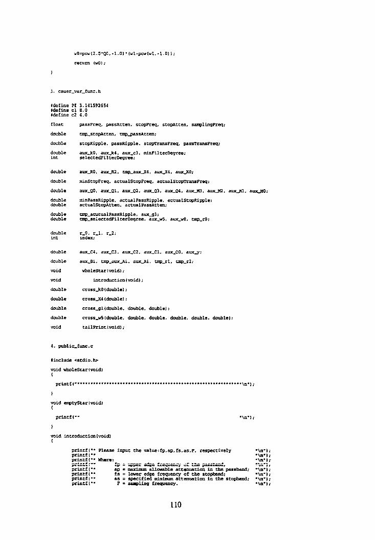
1. cauerjünc.~

2. cauer-catx

3. cauer-var3nc.h

4. pub1icJknc.c

Next we use the MS-Visuai C+t comptier to generate the executable, called cauer-caLexe, and then

run this executable with the MS-DOS window, it wilI give - you the results of the coefficient

caiculation on the user interface.

Figure 4.2 User interface of the coefficients for the Cauer Iowpass filter with the specifications

4.4 The characteristics of 9' order Cauer lowpass filter design

At F:\WD_Filter-De~ignbtlab~sirn~cauer9, we load the MatIab's source files:

1. Two-adap.m

2. wdfiUer.m

3. impulse-respm

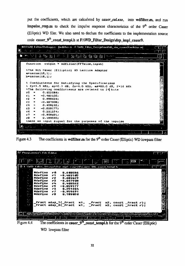
put the coefficients, which are caicuhted by cauer-cal.exe, into wdfilterm, and mn

impulse-resp.m to check ihe impuIse response characteristics of the 9' order Cauer

(Elliptic) WD filer. We also need to declare the coefficients to the implementation source

code ca~er-9~-const-tern~l at F:\WD-F'rlter-DesignwSpPimpI~cauer9. . . .. . .

%The 9 t h Cauer (Ellzptzc] üD Laccree Adaptor a-zeros ( r 8 , i ) ; b=zeros ( 18,l) :

i Caefficiencs f o r Satr~Tp~ng the Speclficscions ; fp'3.5 kHz, a p 4 . 3 d B , fs-4.0 kHz, as-80.0 dB, F-16 kHz %The tollotring coeffrcrents are r t L a C @ d to 24) b i t s rO - 0.603586: t l = -0.483105; r2 - 0.689629: r3 - -0.697908: r4 - 0.409262: r5 - -0.859177: r6 - 0.251224: r7 - -0.959691: r8 - 0.189050: a i %maRe as inDut slanal f o r chc m u r i i o t t s o f the r m n u l s t

Figure 4.3 The coefficients in wdfdter.m for the 9& order Cauer (nliptic) WD lowpass filter

tclefine r 0 0,603586 tclefine r l -0,4831 05 mdefine r 2 0,689629 tdefine r 3 -0,607908 RdeÇine rii 0,409262 SUeFine r 5 -0,859177 mdefine r 6 0,251224 Ldefinc r 7 -0,959691

1 *define r 8 0-189MO

- f rac t a d a p - l t j r a c t x1. j r a c t x2. const - F r a c t r>; - f r a c t adap-2<-fract x l , -Çract x2. const -Fract r);

WD lowpass filter

Figure 4.5 The magnitude and attenuation response of the 9' order Cauer (Elliptic)

WD Iowpass filter

Figure 4.6 The detailed response in the passband and stopband of the 9" order

Cauer (Elliptic) WD Iowpass filter

4.5 Test vector generation for simulation and implementation

To verify the filter for simulation and irnplementation, we need to generate a test vector and pass it

through different types of filters with the Matlab simulator and DSPS6307EVM, respectively.

Test vector description:

fundamental frequency = 500 Hz

sampling frequency = 16000 Hz

test vector size = 2k, i.e. 2048 samples

low frequency component: 0.070sin(oot) + 2.200t)

hi$ frequency component: 0.041cos(12.500t) + 0.062~0~(14.2~0~t)

noise frequency component: 0.024*random(highFrequencyComponent + noiseCornponent) where oo = fundarnentalFrequency 1 samplingE%equency, t is time

Input Signal = lowFequencyComponent+highFrequencyCompon randomFrequencyComponent

Test vector generation:

At F:\WD-Filter-Design\common~~~urce, we run testingSignal_gear.m and plot out the

figures for the input signal in the tirne and frequency domains for Matlab simulation and

DSP56307EVM implementation; this script can also generate data fiIes:

r. matlab-h-inputSignaLdat,

2. pnnt-mcrtlab-Sun-input.daf,

3. print-min-maxqower-SNR.dat.,

The file pht-min-mujower-SNR.dat c m capture the maximum and minimum

amplitudes, which should be within (-1.0, +1.0); this specification is only for the DSP

implementation, real input power, noise input power, and signal-to-noise-ratio (SNR) in dB.

The data file, matlab-sim-inputSignal.dat, is to colIect input signal data in 2048x1 format,

which will be applied for the simulation and DSP implementation of 3 different types of

filters. The reason we need to coIIect the data file is that the noise component is a mdom

one. When we run this script at different times, we will get different input data. So the benefit

of this data file is to guarantee passing the same vector through simulator and DSP EVM. m r v r m ri..- A!oc, k is ï i c c ~ a i tü cüpy Ii iü $ 1 ~ &r~~iury, P : i w ~ _ ~ ~ ~ r - ~ i g n ~ u n a i i a O ~ s i m ~ c a u e r Y ,

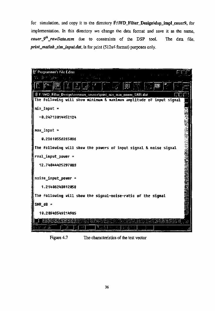
nax-Input =

8.2361 iES6265O96

The following will show the pouers of i n p u t s ignal & noise signal

real-inputgower =

12.74044425297083

noiseinputgower =

1.21406243812858

The following u i l l show the signal-noise-ratio o f the signal

SNRdB =

1 O .2OSWS492l4!?85

for simulation. and copy it to the directory F:\WD_1Filter-DesipWsp-hpl-caud, for

implementation. in this directory we change the data format and Save it as the name,

c~uer-~~-raw~afaasrn due to constraints of the DSP tool. The data file,

print-nrarlab-sim-input,&, is for print (512x4 format) purposes only.

Figure 4.7 The chmctenstics of the test vector

org K." .cauer-9thrawData":$6000

d c 0.1 881363W48962 d c -0. W8l2lW95Uk6 dc II.gP60389747W53 dc 8.05644873843868 dc 0.06987763254867 d c 0.11682196150487 1

! d c il.il88605264g5778 d c 0.14461289199072 d c O. 82255874634048 d c B. iVW2979405599 Uc B.02173321926057 d c O- O2936388429663

i

figure 4.8 The test vector in different formats

Figure 4.9 The test vector in the time domain and frequency domains

4.6 The simulation with a 9a order Cauer (Elliptic) lowpass filter

At F:\WD-Filter-De~ignùnatIab~sim~cauer9, we can run matlab-sim-outputm; it will

show the output signal in the time domain and frequency domains graphicdiy by passing the

test vector, mdlabbsim-inputSignaZ.dat, to the 9' order Cauer lowpass filter.

Figure 4-10 Simulation: Output of the 9~ order Cauer (Eliiptic) lowpass filter

for the test vector

4.7 The compilation of the source codes with gh order Cauer filter implementation

Using the TASKING EDE, we compile the source codes of the 9' order Cauer (Elliptic) lowpass

fitter to obtain the executable, gh-caueflter.abs, which cari be downioaded to the DSP56307EVM.

At F:\WD_Filter-Design\dsp-impI-cauer9, we load the source files:

1. cauer-gh-raw~ata.asnt

2. twoPort-Adap.c

3. cauer-9Yconst-templ. h

4. cauer-91h-main.c

Open TASIUNG DSP563xx EDE Source Compiler, create a project file, called ~hh_cauerFïler.pjt

and add the above 4 source files to the project. Now we can link and build this project and genente

an executable, called 9'h-cauerjilfer.abs, which can be downloaded to DSP56307EVM board for the

implernentation.

4.8 The implementation of the t'ilter in DSP56307EVM with the test vector

Open CrossView Pro DSPS6xxx Debugger, clean up the memory and download

9'h-cauerfiter.abs to the EVM. and run using GO in the CrossView command window.

To collect the input signal data and output signa1 data at the particular rnernory addresses and

using decirnai format, in the cauer-ga-const-templ.h, we pre-set the input data at

X:Ox6000 and the output data at X:Ox8000. To do this, we c m perform a set of commands

in the CrossView command window by using a script file, cailed

dspjo-dataCoUected.cmd, as follows:

Figure 4.1 1 The script file, dsp-io-dataCollected.cmd, to coIlect input and output &ta

En the command window of the CrossView Pro, send the command

"cdsp-io-dataColIected.cmd" which wi11 automatically collect input data from X memory

X:Ox6ûûû and Save it to the fiIe dsp-inputsignal-ruwDcrfaadat and gather output data €rom

X mernory X:Ox8000 and Save it to the file dsp-ou@utSig~aI~rawData.dat both data files

have 5 12x4 format.

Use MS-Excel to delete the symbols in dsp-inputSi~uI-rawDatadat and

dsp-oulputSigna~rawDat~~.& and save as different names, correspondhg to

dsp-inputSigon-l2~4.& md dsp-outputSigm~512~4.d~, cop y them to the direc tory at

F:\WD-Filter-Designùnatlab-sim-cauer9.

Figure 4.12 Data files: dsp-ou@utSignalalr~Data.& and d r p _ n p u t S i ~ ~ w D a i a ~

41

At F:\WD-Filter-Designhatlab-sim-caued, we couId load source code, called

dspjn-out-load.m, and run it. This script wilI automaticaIIy generate 2 data files

dsp-impl-hputSignaLdd and dsp-imp~utputSignddat wi th 2048x1 format. The 2 data

files stand for real input and output data implemented on the DSP56307EVM board,

respective1 y.

Figure 4.13 Data files: dsp-impI~inpirtSignaLdat and dsp-impl-outputSignaLdd

At F:\WD-Fdter_Design\matlabtlsimm~uer9, we load 2 source codes, dsp-impl-inpukm

and dsp-impl-outputm, and run hem individually, which wi l show the real input signal

and the output signal of the DSP implementation, graphicaiiy.

Figure 4.14 Input signa1 in the time and frequency domains with DSP56307EVM implementation

Figure 4.15 Output signal in the time and frequency domains with DSP56307EVM irnplementation

4.9 The cornparison of the input of the test vector with different platforms

Due to the accuracy of the different platforms, such as Matlab platform or CrossView Pro

DSP563xx, we need to verify whether or not the data of input signal is identical with different

platforms. If not, a test vector from DSP implementation expects a re-simulation to parantee there

is no any contamination from input signal.

Open a text editor, such as Programmer's File Editor (PFE), and compare the data file

pnitt-dsp-impl-inputSignaLakt from F:\WD-Filter-Designhtlab-sim-muer9 with the

data file pnnt-matlab-sim-input.dd from F:\WD-Filter-Designkommon-source. And

run the comp-testVect0r.m at the sub-directory of cornmon-source to check the difference.

Figure 4-16 Input of the test vector rit different platforms

Figure 4.17 Input of the test vector at different pIatfom by ninning corne-testvectorm

The input signai is different with different pIat5orms. To minimize the ciifference to zero, we

need to p a s the test vector, dspPimpl_inputSignaL&, which is Iess accurate than

matlab-sim-inputSigriaLdat, to the Matlab platfonn again in order to guarantee that we pass

an identical test vector to both of platforms.

4.10 Re-Simulation by passing the test vector, dsp-impiJnputSipaI

Copy the data file, dsp-impl-inpuiSrgnul.&, overwrite the data file, named

matlab-sim-inputSignuLdr, and run ma tfa b-sim_outputm again.

Figure 4-18 hplementation: Output of the 9' order Cauer mliptic) lowpass filter

for the test vector, &pPimpljnputSignal.dat

4.11 Data cornparison between Matlab simulation and DSPS6307EVM implementation

The final step is to load and run the source code, dsp-simcomp.m. The program is used to

compare the Matlab simulation with the real DSP56307EVM implementation in detaiI. The

cornparisons are as follows:

Input signai in the tirne domain. (data files: print-sim-impl-inpuf_cauer9.fxt, figure

4.19).

Output signal in the tirne dornain (data files: print-mathb-sim-output-cauet9.m

and pniit-dsp-hpbutput-cauer9.m; figure 4.20).

Output signal in the frequency domain (figure 4.22).

Output signal in the frequency dornain with noise amplitude level (figure 4.23).

The spectrum difference between the real and imaginary part of the output signal due

to complex numbers in the frequency dornain (figure 4.24).

The detailed difference between the reai and imaginary part of the output signal in the

passband and stopband. The reason is the same ris in 5 (figure 4.25).

Power cornparison in the time and frequency domains in terms of Parseval's rdations

for apenodic signais (data file: p n n t ~ ~ ~ i m p l q o w e r ~ c o m p ~ c a u e r 9 . ~ t ) .

Figure 4.19 Input Signai in the time domain with simulation and impIementation

Figure 4.20 Output Signai in the time domain with simulation and implementation

d t l a 9th order Cauer YD F i l t e r

0.10813630800088 -0. W812118OBOOO8 1.09683180008080 O.O5644û7008000@

0-06159194624OM 0.W676829022001 0.07270317191478 0-07899291394358 0.06676829022091 0.07270317191578 0.078992m394358 0.07994661314464

with a 9 th order Cauer YD Filter

O.OOû58420009000 0.003451B0000000 0.4118000080000 0.024~160000000

Figure 4.21 The data files of input and output with simulation and implementation

Figure 4.22 Output Signal in the frequency domain with simulation and implementation

Figure 4.23 Noise level specûum of the output signal with simulation and implementahon

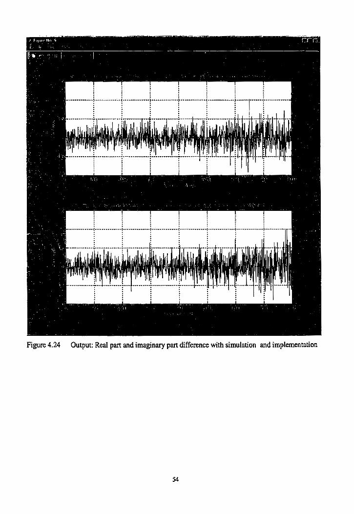
Figure 4.24 Output: Red part and imaginary part diffennce with simulation and irnplementation

Figure 4.25 Output: Real part and imaginary part difference in the passband and stopband

by a 9 t h o r d e r Cauer M F i l t e r i n t e r i s OF Parseual R e a l a t i o n

S imu la t i on i n t i n e donain= I n p u t S i g n a l Power - 13-80ir98W7035438 Simu la t i on i n Freq 6ona inr I n p u t S i g n a l Power - 13,804986971t35437

Inp lementa t ion i n t i n e donain = I n p u t S i g n a l Pouer - 13 -8IW98 W7035438 I m p l e r n t a t i o n i n Çreq d o u i n : Lnput s i g n a i Power - 13,80498WfWS437

S i n u l a t i o n i n tire donain: Output S i g n a l Pouer - 7,22122W8081833 Simu la t i on i n Freq dofuln: Output S i g n a l Pouer - 7.22122W8081834

Imp lenenta t ion i n t ime doœain: Output S i g n a l Poerer - 7-221Z1962165052 I n p l e n e n t a t i o n i n Freq donain: Output S i g n a l Power - 7.2212196216SOS2

The Fol lo ia ing is t o compare power d iF fe rence of ou tpu t s i g n a l between s i m u l a t i o n and DSP imp leaen ta t i on

Output Signal : Power D i i f e r e n c e i n t irne a o m i n - O-OOOOOa859167Bl Output Signal: Power D i fFerence i n Frea dona in - 0~00000085916781

Figure 4.26 Power cornparison: data file, pnnt-~rn-impl_po~er-comp-cauer9~fxf

The values for the input signal of the simulation and implementation are identicai, which

guarantees the= is no impact of different platforms for the test vector.

The vaiues for the output signal of the simulation and implementation in the time domain and

the frequency are very close, which indicate the signals we gathered are correct with respect

to Parseval's relation.

From a Parseval relation point of view, the power difference in the time or frequency domain

between Matlab simulation and DSP56307EVM irnplementation is about 8 . 5 9 ~ 1 ~ ~ . which is

acceptable for the design.

Due to complex numbers in the frequency, we cornpare the output difference between the

Matlab simulation and the DSP56307EVM implementation using the real part and imaginary

part of the passband and stopband, respectively, and pphicaily. We can see the difference is

within 8.0~10" - 1 5 x 1 0 ~ (Figure 4.25). which is acceptable.

4.13 File management and name conventions

There are a number of files including source codes and data files with a variety of names. To make

them more readable for the reader, we introduce the file and directory name conventions and cIarify

the file managemenu with the example, 9' order Cauer lowpass filter design. The examples, a 9 order Chebyshev lowpass filter design and a 7h order Butterworth lowpass filter design use the same

conventions and file tree. We list four figures from a high-level view to the details to show how the

file is managed and explain the name conventions of the directory, source code and data files. We

use boId font in the names for directories or source codes and bold and ltalic font in the names for

the data fiIes or executables.

root directory

sub-directory

Figure 4.27 9Lb Ordcr Cauer Filter Design: Source Code and Data File Management Higli Level Vicw

WD-Filter-Design: directory that is the home directory for the overall filter design. The

directory contains 7 sub-directories. In Figure 4.27, we only show 3 sub-directories for the 9&

order Cauer 1owp;iss filter design.

cornmon-source: sub-directory that includes ail 3 types of source codes and executabks for

the coefficient caiculations of the filter design. Also it covers with source codes and data files

for the vector genentor as an input signal for the verification.

rnatlab-sim-cauer9: sub-directory, cauer9 stands for 9' order lowpass filter. Since al1

source codes in this directory are Matiab codes, it is not only for Matiab simulation, but aiso

for an analysis comparison between the Matlab simulation and the DSP implementation.

6 dsp-impl-cauer9: sub-directory that mems 9" order Cauer lowpass filter design for DSP

implementation only. It contains al1 source codes written using C, test vector in assembly

format, executable, data files, command sctipt and some auto-generated debugging sources

after compilation,

Figure 4.38 9" Oder Cauer Filter Design: Source Code and Data Fie bIanagcment su b-direcîory: cornmon-source

public-func.c: source code, the narne is public functions, which gather al1 sharable functions

for the coeEcient calcuIations with 3 types of filter designs.

cauer-var-funh source code. The name rneans the declantion of the variables and

functions of the coefficient calculations for the 9" order Cauer lowpas filter design.

cauer-func.c: source code which stands for some calculation process of the coefficient

caiculations for the 9" order Cauer Iowpass filter design.

cauer-ca1.c: source code that is the main procedure of the coefficient caiculations for the 9"

order Cauer lowpass filter design.

cauer-cal.exe: executable that can be implemented in a DOS window for the gLh order Cauer

lowpass filter design.

testingSigna1~ear.m: source code, the name is used as a generator for the test vector- It also

generates a data file Cor the characteristics of the signd if the option is ON when executed

pril2t-min-rnaxqower_SNR.dat: data file. Executing testingsignal-gear with print ON

option generates it. The name rneans printing out the minimum and maximum amplitudes

reai signal power, noise power and SNR in dB. Al1 data files in the next discussions wiII be

endosed in appendix section if the name containspint- o r g r i n t

muilab-sim-inputSignaLdaf: data file. It is genemted by executing testingSignal_gear with

print ON option. The data msttnx is 2048x1. This data wilI be as an input signd to pass

through al1 different types of filters with simulation and implementation.

~auer-~~-raw~ata.asm: data file which is exactiy the same as matlab-si~nputSignaLdat

with assembly format for the DSP implementation only. Ii will be copied to the sub-

directory, dsp-impl-cauer9. The data matrix is dso 2048x1.

Figure 4.29 Order Cauer FiIter Design: Source Code and Data Ede Management sub-directory : dspdspimpl_oiuer9

9~cauer~i l ter .~jt: pmject file. The name means a project for the 9' order Cauer lowpass

filter design. It is required by TASKING EDE tool. Under this project, we put ail source code

and data files in it for easy Ioading, compiling, linking, and building.

twoPort-Adap.c: source code. This is a basic hnction to perform a two port adaptive WD

filter routine.

muer-9~lh_const-tmpl.h: source code. The name is the declaration of the constant templates

and basic functions for 9' order Cauer lowpass filter design.

cauer-9~-main.c: source code. This is the main function to execute the procedures for the

9& order Cauer lowpass filter design.

9Qauer~ilter.abs: executabk. It automaticaily be generated by cauer-gch-rnain.c and it is

downloadable to the DSP56307EVM board.

dsp-io-dataCollected.cmd: script. After EVM in running mode, executing this script in the

command window can auto-collecc input data and output data at pre-set memory addresses

and auto-generate 2 data files, we explain them as follows.

dspinputsignal-rawData.dat & dsp-ouCputSigna1-mwDatsi.dat: data files. They are

generated by the above script. The nmes mean the raw data of the input signal & output

signal in the DSP56307EVM implementation. Each file has al1 data addresses with 512x4

formats.

dsp-inputSignal-512x4.dat & dsp-outputSigna1-512x4.dat: data files. The data and size

in each file are exactly the same as in the above, correspondingly, but Excel removes the dl

message addresses. And they will be copied to the sub-directory, matlab-sim-cauer9.

9~ Cauer Filter v dsp-irnpl-inputSignaL&t

Characterizations

1

subdirectory - source code 1-1 uecutable or dni./i*

show figure only

Figure 430 9Ih Order Cauer Filter Design: Source Code and Data Füe Management subdirectory: matlab-sim-muer9

Two-adap.m: source code. This is a basic function to petform a two port adaptive WD filter

routine.

wdfi1ter.m: source code. This is another basic function to implement the routine for the 9"

order WD lowpass filter with defined coefficients.

impulse-resp.m: source code. The name means impulse response. It plots the characteristics

of the 9' order Cauer lowpass filter with impulse response.

matlab-sim-outputm: source code. It is only valid when matlab-sim-inputSignuLht is

Ioaded in the same subdirectory. It can plot the output signal with the MatIab simulation by

passing the test vector to the 9h order Cauer lowpass filter.

print-matlab-sim-output-auer9.dat: data file. The name means print the output data with

the Matlab simulation by passing the 9" order Cauer lowpass filter when

matlab-sirn-output is executed with the print option in the ON mode.

dsp-in-out-1oad.m: source code. Basicaily, it is the procedure to load the input and output

data from the DSP implementation of the 9' order Cauer lowpass filter. It is executable if

dsp-inputSignal_512xQQ& and dsp_oufputSi'gnalal5I2x4.dat are loaded in the same

sub-directory. It also can generate another 2 data files.

dsp-impl-inputSignal.dat: data file. This is the input data More the DSP implementation

of the 9" order Cauer lowpass filter. The data matrix is 2048x1.

dsp-impl-outputSignaI.dat: data file. This is the output data after the DSP implementation

of the 9'" order Cauer lowpass filter. The data matrix is 2048x1.

dsp-impl-input.m: source code. It can plot the input signal and generate a data file for print

only with the DSP implementation of the 9" order Cauer lowpass filter.

dsp-implputputm: source code. It can plot the output signal and generate a data file for

printing only with the DSP implernentation of the 9' order Cauer lowpass filter.

print-dsp-impl-input-cauer9,dat: data file. It means printing only the input data with the

DSP implementation of the 9" order Cauer lowpass filter. The size of the data is 512x4.

print-dsp-impl-output-cauer9,dat: data file. It means printing only the output data with

the DSP implementation of the 9' order Cauer lowpass filter. The size of the data is 512x4.

sim-impl-c0mp.m: source code. It means the comparison between Matlab simulation and

DSP implementation. It compares the simulation with the DSP implernentation in the time

domain and the frequency domain in detail.

print~sim~dsp~power~comp~cauer9.dat: data file. This is the final data file with the

design of the 9' order Cauer lowpass filter. The n a w means printing the power comparison

between the Matlab simulation and the DSP implementation OF Parseval's relation, and to

check the power difference between 2 different ways to irnplement the fiIter-

Chapter 5 The Design Discussion and Conclusions

in this chapter, we wiIl discuss and analyze the whole design procedure described in the above

chripiers.

5.1 Discussion

0 From (3.13) of chapter 3, we have the formula, I r 5 kp, this means we can choose any

value of r within [k,, kp] as a factor to cornpute the coefficients for the Butterworth lowpass

filter design. But this will create a ripple in the frequency response in the stopband. For

example, if we use the srune general specifications as in Appendix B, and choose r=0.0625,

the resulting coefficients rire as follows:

Figure 5.1 The coefficient calculations for a Butterworth Iowpass fiIter

63

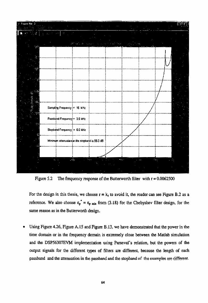
Figure 5.2 The frequency response of the Buttenvorth filter with r = 0.0062500

For the design in this thesis, we choose r = k, to avoid it, the reader can see Figure B.2 as a

reference. We also choose = E, h m (3.18) for the Chebyshev filter design, for the

same reason as in the Buttenvorth design.

Using Figure 4.26, Figure A.15 and Figure B.13, we have demonstrated that the power in the

time domain or in the frequency domain is extremely close between the Matlab simuiation

and the DSP56307EVM implementation using Parseval's relation, but the powen of the

output signals for the different types of frIters are different, because the Iength of each

passband and the attenuation in the passband and the stopband of the examples ~ r e rliffeyenr.

From DSP56307EVM implementation point of view, the input signals of different types of

the filters are exactly sarne, but the output signais of different types of the filters are different

when we apply an identical test vector to the different types of filters. That means the EVM

board doesn't impact input signais at al1 whichever type of the filter is used. The differences

in the output signal are due to different general specifications.

Figure 5.3 The input cornparison with 3 different types of filters

65

Figure 5.4 The output cornparison with 3 different types of fiiters

To andyze the difference of the output signa1 in the frequency domain between Matlab

simulation and DSP56307EVM implementation, we take an FFT of the output signals for L-rL ,,al-- 3 WUI U~GLII&, aiid compare the reai pari anci the imaginary part separateiy due to compiex

number constraints, we c m see the differences are within [5.0~10'~, 1.5~10~], which is

acceptable from a design point of view. This point is demonstrated using Figure 4.25, Figure

A. 14 and Figure B. 12 as references.

5.2 Conclusions

* The explicit formulas developed by Gazsi to design odd-order lattice wave digital lowpass

filters provide a very straightforward method for calculating the coefficients from general

specifications.

The computations are fairly tedious, it requires users to repeat the calculations of the

coefficients when the specifications need to be changed. In this thesis, we developed a

program package and created a friendly user interface for users to easily calculate the

coefficients for three different types of filters, i.e. for Buttenvorth, Chebyshev and Cauer

(Elliptic) filters.

Part of the program package is to verify the characteristics for the different types of filters.

We can easily check them by ninning the scripts, such as impulse_resp.m before the

simulation and DSP implementation.

A test vector cm be passed to the simulation program and the real DSP implementation to

venfy whether or not the high frequency components have b a n filtered out. An appropriate

test vector is very impomt for a successful design.

We used three examples with the above three different types of the filters, and tested them in

a Matlab simulation and in a DSP56307EVM implementation. We verified that the

difference in accuracy in the frequency domain is Iess than 15x10-~, which is acceptable for

design, and then we conchded that the irnpIementation of the explicit formulas to design

lattice wave digital Iowpass filters is reaIizable on a Motorda DSP56307EVM.

From the DSP design point of view, there are always a numberof source codes and data files

to be managed pmperly. We created a method to maintain the 6ies in order in section 4.3.

Furthemore, a more generic package to design filter types other than those used in this thesis

could be developed. For example, computing coefficients would require one program

regardIess of fiIter type; i.e. one program would design any odd-order WDF.

References

[l] A. Fettweis, "Wave digital filter: theory and practice". Proc. IEEEE, vol 74, pp270-327, Feb.,

1986

[2] L. Gazsi, "Explicit formulas for lattice wave digital filters", IEEEE Trans. Circuits and Sys.,

vol. CAS-32, pp68-88, Jan., 1985

[3] J. Wang, "Design of even-order campiex wave digital filters", M. Sc. Thesis. University of

Manitoba, Winnipeg, Canada, 1996

[4] C. Webb, "Design of digital wave-state-variable Iattice filters", M. Sc. Thesis, University of

Manitoba, Winnipeg, Canada, 1987

[5] A. Fettweis, "Digital filter structure related to classicai filter networks", Arch. Elek.

Uebertragrrng, vol. 25, pp79-89, 197 1

[61 A. Fettweis, H. Levin, and A. Sedlmeyer, "Wave digital lattice filters", [nt. J, Circuit Theory

Appl. Vol. 2 pp163-174, June 1974

171 A. Fettweis, "Wave digital filters for improved irnplementation by commercial digital signai

processors", Signal Processing, North-Holland, vo1.16, pp193-207,1989

[8] A. Fettweis, "Digitid circuit and systems" IEEE T r m . on Circuit and Systems, vol. Cas3 1 No.

1 pp3 1-48, Jan., 1984

[9] A. H. Gray, and J. D. Markel, "Digital lattice and ladder filter synthesis", ZEEE, Tram on Andio

and Electroacoustics. vol. AU-21, No. 6 pp-491-500, Dec. 1973

[10] A. Fettweis, "Design of orthogonal and related digital filters by network-theory approach",

AEU, Apr. 1990

[Il] M. EI-Sharkawy, "Digital signal pmcessing applications with Motorola's DSP56002

processot', PTR Prentice Hall, inc., 1996

1121 "DSP56307 user's manuai", Motorula Inc., 1998

[13] A. Oppenheim, and A. Wllsky, "Signais and systems", Prentice Hall, 1996

[14] "DSP56xxx v2.1 Crossview Pro Debugger User's Guiden, Tasking Inc., 1998

Via? K- Ingle: and John G. P i g k i i 'nig&d S i g d Ofnreshg s ing x4%AR,,, RrcctU'Cc!,~,

2000

[16] "DSP563xx EDE Source Compiler User's Guide", Tasking Tnc., 1998

Appendix A The Results of a sth order Chebyshev WD Lowpass Filter

Example: A 5th order Chebyshev WD lowpass fitter design

Genelrl Specifications:

PassbandFrequency: = 3000 Hz

Prtssband Attenuation: = 1 .O dB


Stopband Attenuation: = 40 dB

SampIing Frequency: = 16000 Hz

Rpure A. L User interface of the coefficients for the Chebyshev lowpass filter with the spifications

Figure A.2 The attenuation response in the passband and stopband of the 5' order

Chebyshev WD lowpass fiIter

Figure A.3 nie magnitude Rsponse of the 5" order Chebyshev WD lowpass filter

Figure AA The detailed response in the passband of the 5' order Chebyshev WD Iowpass filter

Figure A S The test vector in the time domain and frequency domains

73

Figure A.6 Simulation: Output of the 5" order Chebyshev lowpass filter for the test vector

Figure A.7 hplementation: Output of the 5' order Chebyshev lowpass fiiter for the test vector

Figure A.8 Input Signal in the time domain with simulation and implementation

Figure A.9 Output Signal in the time domain with simulation and impiementation

Figure A.11 Output Signal in the frequency domain with simulation and implernentaiion

Figure A.12 Noise leveI spectnim of the output signai with simulation and implementation

Figure A.13 Output: Real pan and ircaginary part difference with simulation and implcmentation

Figure A. 14 Output: Real part and imaginiiry part difference in the passband and stopband

1 by a 5 th order Ch~bySheW W F i l t e r i n teras o f Parseual Relat ion

I Simulat ion i n t ime domain: fnput S ignal Power - 13,80498û97035438 Simulation i n Çreq domin: Input S ignal Power - 13.804981197035437

1 Implenentation i n t i r e doaain: Input S ignal Power - 13Al0498097035438 Implementation i n Çreq domain: Input S ignal Power - 13.80498U97035437

Simulat ion i n t ime donain: Output S ignal Power - 6,49919761557241 SimUlatiOn i n Freq domain: Output S ignal Power - 6.99919761557241

Implenentation i n t ime d 0 ~ i n : output S ignal Power - 6,499f9826111585 Lmplenentation i n Çreq d 0 ~ i n : Output S ignal Power - 6,499t9826111587

The Fol lowing i s t o compare power ClifFerenCe OF output s i g n a l betveen s inu la t ion and DSP inplementation

Output Signal: Paver Oif ference i n tine donain - 9-08000964554393 1 Output Signal: Power DiFCerence i n Creq domain - 0,000009o4554346

Figure A. 15 Power cornparison: data file, pnnt-sim-implqower-camp-cheby5.txt

Appendix B The Results of a 7th order Butterworth WD Lowpass Filter

Example: A 7th order Butterworth WD lowpass filter design

Generai S peci fications:

Passband Frequency: = 3400 Hz

P assband Attenuation: = 0.5 dB


Stopband Attenuation: = 55 dB

Sampling Frequency: = 16000 Hz

Figiire B.1 User interface of the coefficients for the Butterworth lowpass filter with the specifications

Figure B.2 The magnitude and attenuation nsponse of the 7' order Buttenvorth WD lowpas filter

Figure B.3 The test vector in the time domain and frequency domain

Figure B.4 Simulation: Output of the 7h order Buitemorth lowpass filter for the test vector

Figure B.5 implementation: Output of the 7' order Butterwonh Iowpass filter for the test vector

Figure B.6 Input Signal in the time domain with simulation and impIementation

Figure B.7 Output Signal in the time domain with simulation and irnplementation

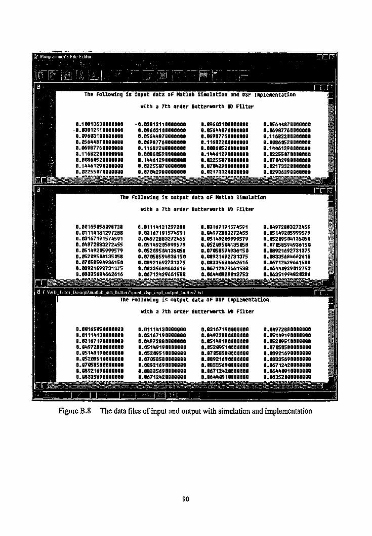
The Following i s output data o f l b t i a b simulation

with a 7th order Butterwrth W F i l t e r

with a 7th order Butterwrth üû F i l t e r

0.06165950808010 0.01114130000000 0.W16719800000~ 9.04972880080000 0.Wll4130000000 0.83167190000008 8.849728BUOE0800 0~85149190008000 0.W1671900000OQ 0.04972880008000 0.851491918000U1 0.05209518000000 0.0497288~001091 0.85149190088000 O.US2û9518800000 0.81058580000800

Figure B.8 The data files of input and output with simulation and implementation

Figure B.9 Output Signal in the frequency domain with simuIation and implementation

Figure B.10 Noise level spectmm of the output signa1 with simulation and implementation

Figure B.11 Output: Real pan and ùnaginary part diffennce with simulation and implementation

Figure B.12 Output: Real part and imaginary part difference in the passband and stopband

I Simulat ion i n t i n e d o u i n : Inpu t S igna l Pouer - 13,80498W7035438 Simulat ion i n Çreq d o u i n : Inpu t S igna l Povcr - 13.80498W7835437

Inp leaentat ion i n t ime domin: Inpu t S igna l Povt r - 18.80498897035438 Implementation i n f r e q domin: Inpu t S igna l Porer - 13,80498097035437

S iau lo t i on i n t ime donain: Output S igna l Pouer - 7,61270924441598 s imu la t ion i n Çreq domain: output S igna l Pouer - 7,61270924441597

Xnplementation i n t i n e d 0 ~ i n : output S igna l Pouer - 7-6127094377h499 Xnplementation i n Freq donain: Output s i g n a l Pouer - 7,632709U77U99

Tne Fol lowing i s t o compare pouer aieference OF output s i g n a l betuecn s imu la t ion and DSP implementation

output Signal: Poiwr DifFerence i n t i n e ao i u i n - 0,000QOOl93329ü2 Output Signal: Pover DiCFerence i n Freq d o m i n - 0-01000919332902

Figure B.13 Power cornparison: data file,pniif,sim-implqower_compu#er7.m

Appendix C The List of the Design Tools

MS-Visud Ci+ 5.0 Compiler

This tool is used to compile the source codes for coefficient calculation, wrïtten in C, it

generates an executable file, such as butter-dexe to calculate the coefficients of a

Butterworth type filter.

Figure C.1 An exampIe by using Visuai Ci+ Compiler

MS-DOS

An MS-DOS window is used to implement the calculation of the coefficients for the

particular type of lowpass filter designeci, which will be run in simulator & EVM.

Figure C.2 An example by using MS-DOS window to run cauer-ai

This tool is used to mn the simulation of the filter design, including the filter charactenstics,

test vector generations, and the andysis of result comparing between the simulation in

Matiab Bc implementation in DSP56307EVM board.

Figure C.3 An example by using Matlab Comrnand Window

TASKING DSP563xx EDE Source Compiler

The tool is a total progrrunming environment that inteptes ail the tools a deveIoper needs to

create, edit, build, and debug an embedded application, including a language-sensitive editor,

easy configuration of compiler, assembler, and linker options, automatic build using MAKE,

custornizable working and application environment. We compile the source code for

implementation with this tool, and genente an executable, such as 9th-cauerfilter.abs,

which is downloadable to the DSP56307EVM board.

. .-

Figure C.4 An exarnple by using TASKING DSP563xx EDE

CrossView Pro DSP56xxx Debugger

CrossView Pro is a debugger For EVM, it provides Features and functionality to help shorten

the debug session, determine performance bottIenecks, uncover additional information, and

test the application, which has multi-viewing windows, code and software data breakpoints,

sing[e stepping without stopping, register grouping, direct memory, C and assembly level

trace and stack tracing, etc. We use this tool to execute the executabIe, such as

9th-cauerfiIter.abs, to run the filter in the EVM board and collect input and output data with

a pre-set vector.

Figure CS An example by using CrossView Pro DSP56xxx Debugger

Appendix D The Feahires of the Motorota DSP56307EVM

Figure D.1 A MotoroIa DSP56307EVM processor

The DSP56307 Evduation Module @SP56307EVM) is a low-cost platform for developing real-

time software and hardware products to support a new generation of wireless, teIecommunications,

and multimedia applications. The DSP56307EVM targets applications requiring a large mount of

on-chip memory such as wireless infrastructure applications. The Enhanced Filter Coprocessor

(EFCOP) cm accelerate general filtering aigorithms, such as finite impulse response (FIR) filters,

infinite impulse response (DR) filten; the EFCOP cm dso adapt FIR filtets as multi-channel filters

used in echo cancellation, correlation, and general-purpose convolution-based algorithm. The user

cm download software to on-chip or on-board RAM, then mn and debug it. The user can also

cfip_n_p~f har&wZT, Y =;Y,~ES ;ty~ ~~Urfgg-:~&$;~ ~ f . &@f&c;üi;Uüg (=,!A)

converters, for product development. The 24-bit precision or the DSP56307 Digital Signal Pmessor

(DSP) cornbined with the on-board 64K of extemai SRAM and Crystal Semiconductor's CS4218

stereo, CDquality, audio codec ideally suits the DSP56307EVM For impiementing and

demonstrating many communications and audio processing algorithms, It is dso an effective tool for

leaming the architecture and instruction set of the DSP56307 procesor.

Figure D.2 The connection between DSP56307EVM and working environment

Figure D.3 The functional block diagram of DSP56307EVM

DSP56307EVM Hardware Features:

high performance DSP56307 core: 100 MIPS (Million Instructions Per Second), 100

MHz clock, data ALU (Anthmetic Logic Unit), 6 channel DMA (Data Memory

Access) controller, on-chip emulation (OnCE) module

enhanced filter coprocessor (EFCOP): on-chip filtering and echo-cancellation

coprocessor runs in parallel to the DSP core

on-chip mernories: 64K on-chip RAM. instruction cache

2 channeIs of 24-bit A/D conversion

2 channeIs of 24-bit DIA conversion

2 ESSI (Enhmced Synchronous Serial Interface) connectors

SC1 (Serial Communications Interface) connectors

The Source Codes for WD Lowpass Filter Design

In the appendix, we enclose al1 source codes (Matlab's, C's and script's) as teferences, Some files

have the same names, but serve different design purposes. To produce a quality visuaiization

(unconvertible between MS-word editor and text editor) for readers, we use a text file format

appended to a11 of them. Each file has a file name and location in the top bar. We split ai1 files into 3

groups in order, according to 3 types of filter designs as folIows:

Group 1: 9" order Cauer (Eliiptic) lowpass WD filter design

Group 2: 5" order Chebyshev lowpass WD filter design

Group 3: 7" order Butterworth lowpass PirD filter design

Note: Al1 files in the File Name List (Ornittedl of Group 3 or Group 3 mean that the codes are - exactiy same as the files in the File Name List IPresented) of Group 1, correspondingly.

Group 1: 9Lh order Cauer (Elliptic) lowpass WD fdter design

File Name List (Presentedl

Gmup 2: 51b order Chebyshev lowpass WD riter design

File Name List (Presented)

File Name List (Ornittedl

Gmup 3: 7Lb order Buttemorth lowpass WD füter design

File Name Li (Presented)

File Name Lit (Ornittedl

1' To calculace the coefficients for Cauer iElliptic1 filters * I

vholeStar(1: printfi" To calculate the coeffieiencs for CauertEllipticl Eilter -\na): introductioni 1: vholeScnr Il ;

printfi'\n\t Passband Prequency: fp = 'l;scanfl'0f',hpassPr~l; ~rintf('\t Passband Actenuacion: ap = 'l:s~~fioOE'.hpassAtteirl:

printft" KiniIirnn filcer Order is Of printft" Please Chwse the Pilcer ûrder N wholeStar~l ; printfi'\n\t The Selected Pilter Ordcr: N = .l: scanf('%d',hselectedPilcerDePrct);printfl'\n'); wholeStar0 :

princE('* The Eilcer order select& is N = Od

else

princft'. The tilter ordcr selected is N = Od

princfl" The actual attenuation in p a s s h d is 0f dB .\n.,acttialPa~sAtcmJ ; princfl" The actiral atrenuation in stopband is 0E d9 *\n',actualStopAttcnl: wfreleStar1) ;

ifl2.index < 101 c iE(r-2 w 100001 printf ('\t\tcoeEficientEOd = Of\n',2'index.r-2) : else printf t'\t\tcoeff icient-Od = Of\n0, 2'fndex. r-2) ;

c iflr-2 w 10000l printf i'\t\tcoeEficient-Od = Of\n'.2'indoc.r-2) ; else

printt ('\II') ; wholeStar[ 1 ; cailPrint ( 1: *&lestar( 1 ;

recurn O;

I

1 I t include *s tdio. iv linclude aiath.b linclude 'cauer-var-frmc-h'

double crossJcO(double kOl

(

double kl.k2. k3.k4;

kl:powlk0.2.0~*s~t~pcwlk0,4.01-1.0l; k2=pow~kl.2.0)*~grtlpaw~kl,4.0l-1.0l; k3=~tk2.2.Ol*s~t(pov~W.4.0l-1.0~; k4=paw(k3.2.01+s~t(powlk3,4.0l-1.Ol;

recurn 1k4);

1

double cross-ROldouble ROI

(

double R1.RZ:

return IXOI:

double aoss,glldouble e_piusStar.double Ki.&uble Ml

c

double gL.gZ.g3:

g1=egassScar*1.0+sgtt~pau~egassS~r~2.0~+101;

g2=gl*Wl+sqrt tpowtg1~MM2.01+l.01 :

J.g2*~+sqrt~powtg2*~.2.0)+1.Ol;

return (931;

J

&le cross-w5 [double wS.double 94. double Q3 .double Q2.double Ql.doub1e QOI

c double w4.w3.w2.wl.w0;

ElaaC

double

àouble

double int

&le

double

double

douiile double

&le Quble

double i n t

double

double

mid

id

double

double

double

double

~ i d

r-O. r-1. r-2; index:

aux-Ca. aux_C3. aux-Ci. aux-Cl. aux_CO, auxy:

auxJi, tmp-auxS. a m i . tq-rl. unp-rt;

who~eStarlvoidl;

introductian(voidl;

crossJO tdoublel ;

crossJ4 tdoublel :

crossgl (double. double, double) :

cross-w5(double. double. double. double. double. double):

tailmint tvoidl ;

printf t"

I l t h e fo l la r ing code is £or debugging purpose only I f p r i n t f L" cauer: 1500.0.2.4100.60.16000 I I p t i n c f ( ' * butterrarch: 1400.0.5.6000.55.16000 I l p r i n t f l " chebyshev: 1000.1.0.5000.40.16000

1

m i d c a i l F r i n t I ~ i d 1 c

pr in t f ( '* printC(" M l c o e f f i c i e n t s a r e quantized t o 24 bits.

%The piece of code is CO ploc ou t input s igna l i n naclab simulation bas i s

c l e a r ;

tormac long:

index = {0:1023)': freqAxxs = (index11281'1000:

dtsp('P1ease choose one O C options: p r i n t - s k i n p u t = 1. show-figure = 2'1; uhich-loap = input(' iay option = ' 1 :

i E w h i k l o o p == 1

d i ' u y prin~qiac labg i I lLinput~dat : inputSigml = msrlab,sint-inputSignall: m a c l a b - s k i n p u t s r i n t = reshape tinputSiqna1'. 512.0 diary otf:

disp('Gnly show input s igna l i n the & frequency domain praphical lyVl:

e l s e

dlspC'ïour option is out of t h e range!');

%mis parcian is to genezate signais a s input and use O-lementacion. which vil1 be as a testing veccor CO

the data rhrough Hatlab Sindation h DSP56307~~ pass different type of the filcers designed

m s i r e = 2048: Half_PFTsire = FFTsi=el2: sampLingPreq = l6000: cime-incemal = Linspace(O.PPTsize-1,FPPsiral;

diary matlabsiatFnpucsig~al.&c; maclab-sincinpucSimiri1 = inpucsignal' diary off;

disp('=e following will show che signal-noise-ratio of the signal'); %dB = 10*1~1Otreal-inpucgowcrfaoi~e~inputgover~ &ary of f :

disp('Your option is out of the range!');

Eigure 11 1

clear:

format long;

FFPsize = 2048; HalfgFTsize = PPTsizelZ; tirne-interval = linspace(O.PFT~ize-l.PFTsize1;

Uoad index.&t index = i0:1023)': tr-is = iindexJ128) '1000:

subplot (3.1.1) :plot (tim=incerval. inputSigoal-arg};axisI [O 512 - .25 .251) ;=id on: title('1nput Signal inplemented in naclab Platfom'): ylabel ('Amplitude' ) :

nibplot(3.1.2);ploc(time~incerval,inpucSigml~rea,'r'I;axis1[O 512 -.25 .25[l:grid on: ticle('1nput Signal iüglemented in Tasking EüE Placforn'): ylabel ('Ar~litude'l :

nibglot(3.L.3):plot(time-inter~al.inpitSipnal-orp-inputSiçnal-rcal:a*isitO 512 -1.5e-7 1.5e-71):grid on: title('1npuc Signal: Amplitude difference with natlab and Taskhg EDE platLorms'l: xlabel('Signd1 in Time ~omain'):ylabeli'~lituda'l:

#&fine PPTSIZE

l&f ine aDDRESS-CRneR_LOCAI.-VAR tdef ine AODRESS-SfnmdTIONJATA l&f ine AûDReSS-Ch~WTPüT

AoDResS-CAuEFi-r.c'=AL-'.mRJ= eqli ADDREsS-CA[nq_OUT~~ W AûDRESS-SMULATIWDAW eqli

ldefine rO 0.603586 &&fine rl -0.483105 Cdefine r2 0.689629 $&fine r3 -0.697908 :&fine r4 0.409262 ldetine r5 -0.859177 #&fine r6 0.251224 #&fine r7 -0.959691 #&fine r8 0.189050

1- 9th CauerlEllipcicl Latcice Covpass Pilter with Specifications'l 1' Ep~3500. ap=ïi.05. fs=4100. as=60, F=16000 *I 1' The Follaring Program is the Inpleaentation for Impulse resy>onse9I sinclude 'cauer-9cLconst-templ-hh Illinclude 'cvoPort~p.c'

-interna1 -fract _X 'pointerSimOata; -incernai -fract _X output [PPPSXZEl -at l A D D R E Ç S - C A ü E R - ~ ~ :

Ilextern -exCernal int J i: -interna1 2 int i;

for ii=O: i <= FFTSIZE-1; ic*) ( IIaIOl=inpuc(il;

dl01 =*poincerShCaca-+:

bl01 =adap-1 (a101 .alIl. c01; b[ll=adap-2laIOl .a[ll.rO): altl=b[Ll: a[61=b101:

bt8l=acidp-L~aIaI .a[91.r41; bl91=adap-ltal81 .a[91.r4): a191=b[91: a[71=blBI:

bl61=aOap-ttat61 .a[71.r3): bl7l=adap-2taI61 .al71.r31: all4l=bibl;

bll61=adapJlalL61 .afl71 ,dl; b~l7I=adap-i!lal161 .a[Lll,r81: altll=b[lfl; aI151=b1161:

bll4l=a&p~la[L41 .a[l51.r7): btl51=adap_2laCl41 .ai151 .cl):

I' Input for Lavnr Section *I a[2l=aIOl;

bl4l=adap-l(a[Ol .a[51.r21: b[SJ=adap_2ta[41 ,a[51 ,r21; aCSi =bl51: aC3I=bt41;

1 Data as impulse respoose *I output[il=0.5*ibtl4l+bllOl);

1' Punction's Definition for Isc Elcnrne ot 'hm-Port Adagtor ' I

l l f l o a c adap-l(Cloat ri. floac x2. Eloac rl

-iracc adap-11 -£race XI. -frace x2, coast -tract r)

[ l l f l c d ~ t; l lfloat yl;

-fracc c: -tract yl;

1' ~ c t i o n ' s Definition Eor 2nd Elemeat of Tau-Port ~ p c o ~ '1

-5ract adap-2I -fracc xl. -fracc x2. const -fract cl

return 1 ~ 2 ) ;

1

0- piece of cade is CO ploc out input signal in OSP56307M -1-tation b s i s

clek-;

formac long;

%lwdfng input signal for print purpose

fprintf(EidJ.' OIO.14E 420.14i 420.14f 420.14f\n'. ... inputSignallil.inputSignal(i+ll.inputSignalti+2l,inputSignalti+3~1;

elae EprincL (fid-1, ' tl0.14E b20.14f 620.14f t20.14E\nD, ...

inputSigaaliil.inputSignal~i+ll.uiputSignalti+2l.iDputSigaalii+3ll: end

end

Éclose i f id-LI;

disp('0nly show input signal in cime h frequency demain graphically'l:

else

dispt'your option is out of the range!');

end

subplotl3,l.l) ;ploc(time_interval.dsp-input) :axisi [O 512 -.25 -251 l ;g+d on; ticlei'Tise ~omain: Input Signal for 9th Cauer IEllipticI DSPS6307EVn uirplemuitation'l; ylabel('%uplitude in The domain' 1 ;

nibploci3.1,2l;ploctEreqA*is,unpl1025:20481/HalfJFPsize.'r'l;~d on: title('Overal1 Spectrum: Input Signal for 9th Cauer (Ellipcicl DSPS6307M implementation'l; ylabel i'%uplitude'l:

subploti3.1.3) ;ploc(frcqAxis.unpi1025:2048l /HaIf-PPTsizc, 'm'l ;sis1 10 8000 O .O061 1 ;grid on; title('N0ise kvel Spectrrmi: Input Signal for 9th Cauer (Ellipcicl DSP56307EVK implemencation*l; xlakli'fceqxncy Damain: Hz'l;ylakli'Amplitude'l;

\The piece of code is to plot out output signal in DSP56307FlM inipLamICaCioa bsis

t o m t long;

index = 10:10231 '; t-is = lindu1128l*1000;

Ol~dfng output signal for print purpose

disp('P1ease choase one oE options: print-a&output = 1, ahai-Cipure = 2'1: which_twp = inputt' my option = '1 ;

iTille-1 = ~print-&p-tnPl-0~tput~~a~et9~~1t~; Ei41 = EopenliTitle-1,'wr'l: EprintElficiJ. '\t\t The Eollowing is output data of DSP rmplmentation\n\n'l; EprintClfidJ. '\t\t\c with a 9th order Cauer WD Pilter\nb\n'l:

for i = 1:512

iE outputsignal [il c O EprintflficLI.' 010-ldf 020.14f %2O.I4E %20.14f\n'. ...

nitputSigna1 (il .outpicSignaLti+ll .outpucSignal(i+21 .outpitSignaZ ti+31 1:

displ'hily show output signal in cine h freguency domoin qraphically'):

else

disp('Your option is out of the range!');

end

subplotl3.1,1l:plotlcime~interval.dspdsp~cpit~:axis(t0 512 -.15 .lSIl:grid on: citle('Timz Damain: Output Signal for 9th muer [Ellipric) DSP56307ëVX inplementacion'): ylabel ('Amplitude in Time domin' ) :

subplocl3,1.2);plotlfreqAxis,~(1025:20481/Balf-~size,'r'~:~d on; citlel'overall Spectrum: Output Signal for 9th Cauer (Ellipticl DSP56307EVM implementacion'l; ylakl t'Amplitude' ) :

s~Loc(3.1.3~:gloc(freqAxis.~(L025:2048~/KalfJ~size,'n'I;axist[O 3000 O ,006l):grid on; citlr('Noise Level Spectrum: Output Signal for 9th Cauer (Ellipcicl DSP56307EVn implernencacion'l; xlabel('Frequency Domain: &'):ylakl('Aiÿplicude'):

$The prcgram is CO l m d the &ta oE input and oucput signal with DSP563075~M implcmcncation

clear;

format long;

subplot(2.l,ll;plotlt~,interval.&p~iripu~Signal.'r'):~s~IO 512 -.25 -2Sll;grid on; ticle(~mpuc Signal of 9th Cauer (Elliptic) DS~563070R3 Implmieatation in T m Danuiin'); ylabel('Amp1itude');

nibploc(2.1.2I :plot(tfme_interval,dsp_outpitSip~l) ;&SI IO SI2 -.25 .2SI l :grid on: citle('0utput Signal of 9th Cauer (Ellipticl DSP5630fEW -1-tation in Time Danuiin'); %label ( 'Signal in Time Oomain* 1 :ylakl t 'Anplitude' 1 :

subplot(2.1.1) :ploc~fIeqAxia.tmp,l1(102S:2048lI~1Lpprsize,*r' ;grid on: citle('1nput signal of 9th Cauer (Elfipticl DÇP56307EVü Enplmencation rn Prequency Damain'): ylabelt 'ampli tude' 1;

subplot(2.1.2l :plot(freqllxis.tmp,22 (1025:2048) / ~ I a l £ ~ s i z e l ;@d an; title('0utput Signal of 9th Cauer (Ellipticl OSP56307EüH Implemurtacion in Frequency Dcimafn'l: xlabell 'Signal in Frequency Damafn: Br' : ylabel ('Amplitude' ) :

subplot~2,L.l);plot~freqllxis.~m0_11~1025:2008)/HalfgFPsize.'r'):axis~[O 8000 O -0061);grid on: title('Noise Level Spectrrmi: input Siguui of 9th Cauer (efliptic) EP56307EVM ~lcmentation'l: ylabel t 'Amplitude' ) ;

dispi'please choose one oi options: not-load_dsp_io-&Ca = 1. 1wdAsp-io-&ta = 2'); '&ch-hop = input(' my option ' 1 ;

diary &p--1-inputSignal.&t; dsp-inputsignal diary off;

diary &p--1-outputSignal.&t: dsp-outputSigna1 diary off;

disp(' <dsp-kapl-inputSigxd.&t> is input data Emm EVH implaauicatian.'): dispt' cdsp--1-outputSignal.dat> is output data frcan EVX implementation:);

else

disp('Your option is out of range!');

end

%The charac~oriracians of the 9th Cauer (Ellipcic) lowpass latrice filter

clear: fomac long;

FFTsize = 2048: cime-interval = 1inspaceiO.PFTsize-1.PrPsize);

impulseKnput(1) = l:i~ulseInput(2:FPTsizel = zeros~FPPsite-1.1); impulseOucput = vdf rlteriPFTsize, i ~ s e L n p u t 1;

subplot(2,1.1):scabitiar_intenral,i~lsauitput. 'r');axisl[0.32.-0.2.0.4II;grid on: tltlel'Impulsc Respanse of che 9th Cauer (Elliptie) lavpsss Pilter');

subploC~2.1.2l;pLot~fftshift(abs(fEtl~~ulscQutput)l~ll;axfs~[500 1550 0.96 1ll:qrid on; trtle('Iupu1se Prequency Speccrrmi of Che 9th Cauer (Elliptic) tawpass Pilter'l;

s~bplot(2.1.l~;ploc(frcg~xis.~stnagnfeute):sxis~10.8000.0.ll):Qlid on; tsxt(4500.0.75.'~ruriptfng Prequency = 16 kHz'); text(4500.0.55.'passband Preaueno = 3 .5 kiiz');

subplot(2.1.2) :plot(freqAxis. impilseAttuiuationl ;arislC0.8000.0.200I) ;grid on: cexti500.9O.'Samplhg Prcquency = 16 kEz'1: text~500.70;Passband Prequmcy = 3.5 Mz'); torc(500.50,'Stopband Repuency = 4.0 ~z'):tat(4100.50.'Miokmnn actenuation ia the stcpband is 80.0 dB'); titlet'Attenuation Respo~e of the 9th Cauer (Eîlipticl Lavpass Filter'l; xlabefI'Frequency in Kz*);ylabell'Attenuation in dB');

~lot13.1,2);p1ot(frcqAxis,~seAttmuationl;a*istCO 4000 O 0.4l);grid an; text(550..35.'&dmm attenuation in the passbarid is 0.3 dB'): t u t (2200. -35. 'Passband Prequency = 3500 Bz' ) : title('Passband Atcenuatian Resgonse of the 9th Cauer IElliptic) Lovpass Ptlter'):

subploc(3,1.3);ploc(freqXxis.~1seAtten~dtion~;~is3500 BO00 60 2001);grid on: cexc~S200.170:~inimrnn actenuation in the stopband is 80.0 dB-1; ;ex (5200.150. 'Stopband Prequenc/ = 4000 Hz' l ; ticle('Stopband Accenuation Respan5e of the 9th Cauer IEllipcicl Lobpass Pilcer'l; xlabel('Prequency in tfz'l;ylabel('Attenuation in dB');

#The piece of code is CO ploc ouc output signal in Xaclab simulation basis

clear;

t o m t long;

index = (0:1023)': EreqAxis = ~index/128~*1000:

tloading output signal for princ p w s e

disp('P1ease choose one of options: printg~oucput = 1. show-figure = 2'1; nhich-Loap = input ( ' my option = ' ) ;

if rhichJoop == 1

z'ïitle-1 = 'princguclab~si~outputtcauer9.~c'; fid-1 = fopen(rTic1e-1,'wr'l: £princE(Eid-1. '\t\t The Eollowing is output data of Maclab Sinailation\n\n'I; tprintf(fid.J. '\c\t\t with a 9th order Cauer WD PLlcer\n\n\n'I;

for i = L:S12

if oucpurSimia1 (il s O Eprincf (fici-1.' %lO.ldt U0.14f %20.14f t20+14f\n', . . .

ourpitSignal~il.oucpueÇiqnal~f+l~,oucput5igaalli+2~.out~~Si~lli*3lIz else

tprintt (fici-1, ' 310.14f o20.14f 120.14f i20.14£\n'. ... outpucSignal(il,aucputSi~lIi+1),oucpucSi~lli+2~,aucpucSignal~i*3l1:

end

fclosclfihll;

elseif which-loop == 2

disp('0nly show oucput signal in tima & Lrtqucncy domain graphicaily'l;

else

disp('Your option is out of the ranger'):

end

subplot(3,l.2):ploc(Er~s.~(1025:2048l/Half_WTeize.'t'l;gcfd an: title('0verall S p e c w : Output signal for 9th huer (Elliptic) Hatlab Sinulatian'l; yfabef I'Amplftude'I;

%This program is CO canpare with the shlatiou h DSP iniglemontation in iarlti-uays

clear:

format long;

W s i z e = 2048; tialfgmsize = PFPsizel2: cime-interval = linsgace10,PFPsize-1,PFTsize):

0load index.&c index = i0:1023l': freqhis = lindut/128)*1000:

%------------------------------------------------------------------------------------------------------------ a-s zone is co load simulation h implementation &ta

aaclab-outputSigna1 = wdf ilter IPFTsize. dsp-impl-inpucsignall :

\-----------------*----**-*-----------*----------------------------------------------------------------------

??!IF~ seccion in ta compare vath c'Ce real part and imginary part between Hatlab r DS25630fFJX. respac:;vely

subploc(3.1.1) ;plot ~time,interval,matlababmtpr~SisaaIl :axisf [O 512 -.15 -151 I :grid an:

ticle('Actua1 Output Signal in Time m i n with 9th Cauer (Elliptic) Haclab Simulaticn'): ylabel('Anip1irude'I:

subplot~3.1.2):plot(tiw~interval.dsp~~l~out~tSipna1.'r'l:aui~I~O 512 -.15 .15lI;grid on: cicle('Actua1 Output Signal in Time Domain with 9th Cauer [Ellipticl DSP56307eVM ~lemwtntian'l; ylabel {'Amplitude' ) :

subplot (2,l. 11 ;plot (frepAxis.mtlab~10~~~~~0~tp1tSigaal( 1025 :2048l IblfJPTsize. ' r' l ; grid on: ticle('The Spectrinn: Accual Output Signal with 9th Cauer (Ellipticl üdtlab Similation'l: xlabel('Prequency in Hz'l;ylabel('Amplitu&'l:

subplot(2.1,2l;plot(frepAxis.&pglotPPP_outputSignal(1025:20481IAalf~Pfisize); grid an: CitleI'The Specrrum: Xctual ciutput Signal with 9th Cauer (Ellipticl DSP56307EVK Implcnrntation'l; xlabel('Prequency in nt'l:ylabel('Amplitude'l:

axisi [ O 8000 O :0041 tq&d on; trcle('N0ise Level Speccrum: accual Output Signal with 9th Cauer (Ellivtic) mtlab Sinutlacion'): xlabe1i'Prequency ln ~z'l:yLakl('Amplitu&'l;

subplot(2.1,2~;pLot~fr~is.&p~l0t~~0~tputSignal(l025:2048lIAalt~sizel; axist[O BO00 O .0041):grid on: title(*troise Level spectrum: Accual Output Signal with 9th Cauer IEllipticI DSP56307EVM -1-cation'); xlabel('Prequency in Ht'l :yLabel ('Amplitude'l ;

s~lot~2.1.II:plot~freqiius.ditf~realParc~PFP(lO25:2O48l/HalfJFTsize.'r'l;prid on: title('The Output Speccnun Difference in real part betwecn 9thCauer (Ellipticl Sindation and Lniplemcntatim'l: xlakl('Prequency in Hz'l;yLabel('Amplitude'l:

subplot (2.1.21 :plot (freg~xis,diff~imagPart~~~1025:2048l lüalf-Pfisize) ;grid a; title('The htpuc Spectnun Difference in h g part between 9th Cauer (Ellipticl Simulation and Implementatien'); xlaklt'Prequency in Hz'l;yLabtl('Amplicu&'l:

nrbplot(2.2,1l;plot~frcgi\*is(l:449l,diff~realPa~~(l025:1473lIBalf~PFTsizel; ticlel'9th Cauer lElliotic1 outmit real m r t diff in mssband'l;

NbpLot(2.2.2l;pLot(fregAxis(64L:lOZ4~.diff~reaLPartgPT~1665:2048)Iblf~~ize.'r'~; titlet'9th Cauer (Elliptic) outpit real part diff in stopbaod'l: xlak1I'Prequmcy in Hz') ;ylakl('Amplitude'l :grid on: subpLoc(2.2.4) :pIot(fr~is(641:l024l .diff_hgPar~m[l665:2048)Iblfg~~size, 'r'l ; title('9th Cauer (Elliptic) output h g part diff in stopband'): xlakl('Prequmcy in Hz' l :ylaklt'Amplitude' l :grid on;

disp('P1ease choose one O£ options: trac--data = 1. printsovv-coirp = 2'1; *&ch-loop = input t ' my ogtion = '1 ;

if whik1oop == 1

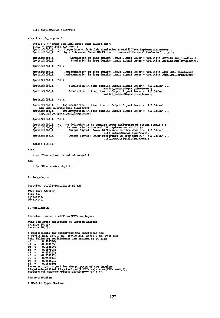
iTitle-L = 'print-s~implgower~camp~ca~er4~ert': fihl = fopen(iTit1e-l.'wr'l; fprincf(fi&i. '\c Cmpuison wich HaClab shlation & DSP56307EVn ~lementation\n\n*I; Eprintftfici-1. '\t by a 9th order Cauer WD Pilcer in terms of Parseval Realacion\n\n\n'I;

fprincC(fidJ. ' Simulation in cime daanin: Input Signal Power = OlO.L4f\n*.matlabg~ch~overl; fprincf (firl-1. ' Simulation in freq daiiain: Input Signal Pcwer = 0lO.L4f\n'.matlab-s~freq~ower1;

fprincl (f ici-1. ' \n' ) :

fprintL(fiL1. ' ~lenientation in timc domain: Input Signal m e r = 010.L4E\n'.dsp-impl-time~ower); fprincf(fi&i. ' implemuitation in freq domain: Input Signal Pmer = 010.L4C\n'.dsp-impl-freq~orer~;

Eprincf ( f iai. ' \n' 1 ;

fprincf ( f id-1. ' Shlation in cime dowin: Output Signal Power = 010.14f\n',.-- maclab-outputSiw1-timepower);

Epr'hcf if idJ, ' Simulation in freq -in: Output Signal Power = %lO.l4E\n', ... maclab-mcputSipna1-Ere~Parer};

Eprincf (fidJ. '\nPl;

Eprincflfici-i. ' implemencation in c h dowin: Output Signal Power = %10.14f\n'. ... &p--1-oucputSigna1-timepawer):

fprincftfid-1. ' miemencation in freq domain: Output Signal Power = %10.14t\n'. ... &p--1-outputSigna1-freqpwer);

fprincf ( fid-1, '\n') :

fprincf fprincf fprincf

fprincf

ifrd-1. '\c The Eolloving is CO c m r e paver difference of oucpuc slgnal\n'I; (fici-1. '\t\c bec- simulation and DSP ~laœntacion\n\n'l: tfid-1. ' Oucput Signal: Pawer Ditference in cime domain = 01O.l4f\n'. ...

aiff-outputSignal-timeP0wcr~ i Ifid-1, ' üucput Signal: Pwer Ditference in freq darain = 810.14f\n'. ...

ditf,outpucSiqml,fregPwerl:

dispI"four option is out of range!'):

funccion tbl.b2liPwo-adavtr.al,a2)

funccion oucput = wdEilter(PFTsize.input)

%The 9ch Cauer (Ellipcic) WD Lattice Adaptor a=zerosll8.1); brzeros (18. 1) ;

O Coefficients for Sacisfyfng che Specificatioas O fp3.5 küz. apd.3 dB. fs4.O kRz. as=80.0 dB. F=16 kHz One follosrfng coefficients are relaced co 24 bits rû = 0.603586: rl = -0.483105: r2 = 0.689629: r3 = -0.697908: r4 = 0.409262; r5 = -0.859177;

= 0.251224: r7 = -0.959691:

for n=l:FFTsize

8 Goes to ripper Section

0 CaLls the function creaced

iblll .b(2) IiRuo-adaplrtl.ail1 .a121 1;

0 Nexf State

ai21=b(2);

0 Connection Conscraint

a Goes CO m e r Section

a13)=alll;

b mds Lover Section

OEigure(1) ;stan(outputJ ;axisl [O 70 -0.2 0.41 1 ;grid on;

wholeStar I I ; printfl'. To calculate the coeffieiencs Eor Chebyshcv Eilter *\n*) ; introduction 1 1;

princft" Xfnimum filcer Order is \ £ nrintE1" Please Choose the Filter Oder N bhole~tar0 ; printfIs\n\t Rie selccted Pilter Ordfr: N = ' 1 : scanfl'0d'.hseIeccedPilter~ce):pruicE~'\n'):

wholestar O ;emptyScarll; printff" The actual attenuation in passband is 0f dB *\n'. pass~tten-star) ;

printfl" The actual accenuatian in stopband fs Pf dB *\no. stopâtcen-star) : empcfitart l ;wholeStarll;

1 if tr-1 r -10000 && r-1 c 0) printfl'\t\tcoefficientttd = 0E\n'.2*index-L.r-1); else printf t'\t\tcoefficicat3d = tE\n0. 2.indtx-L. r-1) ;

1 else ( if fr-1 > -10000 && r-1 c O1 printf t'\tltcoefficient~0d = 0f\n'. 2*foda-L.r-1) ; else prinrf t-\t\ccoefficieuttM = Pf\n'.Zbindex-LrJl ;

1

c itlr-2 > 100001 printf ('\t\ccoefficienttOd = 0t\n'.2'index.r-2~ ; else priotfi'\t\tcoefficiurtSd = %f\a',2*index,r-21;

>

t&f ine ldefine tdefine

t l o d ~

do& 1 e

deuble

dcuble

:nt

ddubIe

double

double

int

double

=id

void

vuid

void

awrJc0. aux-kl. i w - c 3 , minFilterDegree;

index:

#Qf ine ADDReSSReSCHEBï-LOCAtOCAtVAR OxlOOO t&f ine AûtiRESS_ÇMIILATIONJATA 0x6000 #define ADDRESS-QfEBYYOUTPüT 0x8000

c- -*- o u - L I L - / T h e follawiag coefficients are related to 24 bits*/

Idefiae rO 0,675837

a ~ h e piece oE COQ is to plot out input signal in DSP56307EWX implementation b i s

clear;

E-t long;

Load dsp--1-inpiUiqnal.&C;

index = 10:1023)': freqAxis = Iindex11281*1000;

%Loading input signal for print p-se

dispi'?lease &ose one of options: printgkinput = 1. show-figure = 2'1; uhich-hop = inpucl' my option = '1 :

iTitle-1 = 'print3irQ-1-inputC&eby5.txt'; EidJ = LopeniiTiCle-1. ' w r ' I : CprintflfidJ, '\t The Eollowing is input data of Haclab Sfnulation and DSP ïmplcmui Éprrntf(fidJ. '\c\c\t vith a 5th order Chebyshev WD Pilter\n\n\n'l:

end

disp('0rily sha* input signal in tirna & frequancy damain praphically'l:

dispi'uout option is out of the rsnqei ' 1 ;

end

subplot(3.1,11;plotttima,intcnmi.~-inpur):ads([0 512 -.25 .251l;qrid on: ritlc('Tfme kamin: Inpvt Signal for 5th Cheby~hev DSP56307EVM impiCaWlCXfon'); ylabel ('Amplitude in Tira domain' 1 ;

subploc~3.1.2l:ploclfr~s.~il015:2048lI~lfJ~size,'r*l;grid on: ciclet'overall speccnsm: Input Signal for 5th Chebyhev DSP56307EW ~leuentatim'l; ylabel L'xmplit~de' 1 ;

subplot~3.1.31:plot(f~s.~îlOZS:204811~al~size,'m~):aris[[O BO00 O .0061l;grid on: ticle('N0ise Level Spectntm: Input Signal Eot 5th Chcbyehev üSP56307EVü impl-tation'); *label ['Frequency Demain: üz' 1 ;yiaki ('Amplitude' 1;

%The piece of coüe is to plot out output signal in DSP56307FJK fmpleaentatian basis

load dsp-impl-inpicSisnal.dat: load asp-impL-outpucsigIlal.dat:

PFTsize = Z048: KalfSFTsize = FFTsizelZ: cime-inteml = lins~ce(O.PFTsize-1.PFTsizel;

%loading output signal Lac princ purpose

disp('Pledse choose one of options: p r i n t 3 k O u t p ~ t = 1. show-figure = 2 ' ) : uhichJoov = inpucl ' my option = ' I :

iTicle-1 = ' ~ r i n t - & p - ~ i - o u t p u t - c h ~ . t w c * ; EiàJ = fopx l iTi t le-1, ' w r ' ; Eprintf(fidJ, ' \ t \ c The foltopring is autpilt data of DSP Impleaencation\n\n'); Eprintftfid-1, ' \ t \ c \ c trich a 5 t h arder Cixhyshev WD Filter\n\n\n1);

else fpnnrf (€id-1. ' 010.14f 02O.f~f 920.10f fi20.l4f\nP, ...

oucputSi~l(i~.~tputSiqnal(i+l).outpi~i~l(i+21.outpitSignal(i+3)); end

end

disp('0nly s h w output signal in cimi L Erern<enc{ damain graphical1y'):

displ"iour opcion is o u t cf the range! '1 ;

subplot(3.1.3~ :plot(frcgAns. ~(1025:20481 lüaltfprsize, 'm.) ;&s( [O 8000 0 -0061 1 ;grid on: title('Noise m l Spectrum: Output Signal for 5th Chcbyshtv DSP56307m implemcnracion'l; ItlaklI'Vrequency m i n : Efz');ylakli'A~~plitude'l;

%The progrrarn is Co load the data of input and output signal uith OçP5630ïFJH ~laaentatiori

kload Ur.&: index = IO:1023l'; EreqAxis = tindex/128) '1000:

subpl0~(2.i.r);plot(time_interval.dsp-iaputSionai.'r'l:axist[O 512 -.25 .251l;prid an; title('1nput Signal of 5th Chebyshev DSP56307BRI Unplementation in Time Domain'); ylabel ['dmplitude' :

subplot(2.1.2) ;plotttinie-intenral.&p,outpttSignall :&si [O 512 -.25 -2511 :grid OU; title('Output Signal of 5th Chebyshev DÇP56307EVH Impl-tation in Tire Damain*): xlabel ('Signal in Time Domain' 1 ;ylabel 1' Ampiitude' ;

subploc (2.1.1l :plotlEreqRvis. cmp-11 l1025:2048) /Salt-PFTsize:r'I ;grid on; title ('Tnpuc Signal of 5th Chebyshev DSP56307EVn Iniplemenmtion in Frequency Danmin' 1 ; ylabclt'rimplitude'):

subplot(2.1.2~;plotlfr~s.~~22il025:2048)I~lfgPPsize~;grid on; title('Oucput Signal of 5th Chrbyshev DSP56307EW Iniplanencacian in Prequency Dowin'I; xlabel('Signa1 in Prequencf Dcmiain: Hz'l:ylabell'Amplitudc');

subplot(2.1.ll ;p lo tIEreqi lx i s .~ - l1 i1025:2048l /HaIf-PFTsize, 'r') ;&SI [O 8000 O .O061 ;grid on: ticle('Noise Level Speccrum: Input Signal of 5th Chebyshev DSP56307EVèf Iliipimwtation'); ylabel ( 'Amp1i:ude' I ;

dispf'please chwse one of options: noc,loahdsp-io-data = 1. loaLdsp_io-data = 2 ' ) ; which-loop = input (' my option = ' 1 ;

%The charactorizations of the 5th Chabyshw iowpdss lattfce filter

claar; format long:

ploc( treqhis. ixguls&ttenuatian) :ais 1 [O. 8000.0.1201 1 :-id on; cexr(500,190.'S~ling Prequency = 16 W'l: cu(t(500.170:Passband Prequmcy = 3.0 kHz'): textï500.~50.'Sta~band Praucacv = 5.0 m'l: cext(500,130:~iaimilm att&cf& in the scopband is 40.0 dB-1: title('~ttenuatiaa Responac ot the 5th Chebyshev Lowpass Pilcer'l: xlabel(*Prtqueacy i n ~Iz'):yiabelt'Attenuation in & ' I :

figure 13)

piot(~r~is.imgtrlse~agnituce,'r+1:axis([0.8000.0.11):i~rid on: text(4500.0.75. 'Sampliog Frequency = 16 k k ' l : t u t (4500.0.55. 'eassband Prequency = 3 .O Mz' 1 : ttxt(4500.0.35. 'Stopbaad Frequency = 5.0 kBz' l ; citlel'nsgnirute Response of the 5th Chebyshev m a s Fflter'l; xlabel( 'Prequency in Hz' i ;ylabel ('Magnitute in dB' 1 :

subploc(2.1.Ll :plot ~ft~is,impulseMqnitutal ;axislIO 3500 0.85 11 l :grid on; tutc(ltOO,O.8~5, '9aqnitute cespanse in the pusband' l ; titlel'eassbmd Wgnitute Respanae of the 5th Chebyshcv Lcwpass Pflter'li ylakll'nagnituce in dB'!;

subpIoct2,1.21;plottfr~is.impils&ttanuacfonl;axisitO 3500 O 1.2l);grid on; c~t~1050.1.I:naximm atteauatioa in the pasaband i s 1.0 dB*): titlel'eassband kttcnuatian R e m s e of the 5th ChebyShev bmpass Qiltcr'l: ylabeLl'Atcenuacion in dB');

%The piue of ccde i s ro plot out outpur sigaal in Hatfab almulacion -1s

clear:

f o m t long;

maclab-input = matlab_si~inputSigMr:

index = {0:1023)'; f r w s = (indwc1128) '1000:

maclab-output = vdfilcer1PFTsize.matlab-input);

alaading output signal Cor print purpose

disp('P1ease ciiwse one of optiansr print-skoutpuc = 1. show-figure = 2 ' ) : whiciCloop = input t ' m/ optiaa = 1 :

iTitle-1 = 'print_aatlabsim,outputtEiieby5 .txc' ; fiàJ = fopentiTitleJ.'wr'I: fprintf (fici-1. '\t\t The followiag is output data of Ihtlab Shrdation\n\n') : fprintf (fici-1. '\t\c\t vftb a 5th orüer aiebyshev WD Pilcer\n\n\n') :

for i = 1:512

displ'0nly s h w eucmt signal in t i w 4 frequency dnmain graphically'):

else

dispi'Your option is out of Che range!');

end

~lac(3.1.1):plot(t~-in~erva1,~dab~outguti;~sitO 512 -.1S .15l);wid on: ticlc['Th m i n : Outpur Signal for 5th Chebyshev mclab ~imulation'l: jrlabel( mAmpLicude in T i w donuiin' 1:

subplot(J.1.2l ;ploc(f~Axis,uip(1025:2048) lüdlf-FFTsire. 'r') ;grid on; citle('ûveral1 Spectrum: Oucput Signal for 5th Chebyshev Matlab Sinailacian'l; ylabel(';\mglitude'~;

subploc(3.1.31:p1otlfrcqAxis,tirrp(1025:20d8iIfEalf,PPPsize.'m'~;axisi[O 8000 O .00611:grid on; titletaNoise Lerel Spaccntm: Output Signal for 5th Chebyshev MaClab Simulacion'l: xlakll'Frequency Douain: Hz');ylakli'Amglicude'l;

\This program is CO cangare wich the siimtlation & DSP implanencacion in mulci-vays

ciear:

f o m t long:

Uoad index.dar index = 10:1023l': freqhis = 1index1128I .LO00;

t---------------------------------------------------------------------- %fie section i s CO c v e wiCh the powers io t ime daDain & trcquaecy drimain. using P a r s e a l ' s Relation

subploc(3,l.l);plot[time_intervd.~tlab~s~in~cl:axisî[O 512 -.25 -2SIi;grid on: cicle('Actua1 Input Signal in T h Daaain with 5th Chehyshtv Matlab Çidaticn'l; ylabel ('Amplitude' i ;

subploc13.1.2) :plot(timt-ioterval,dspdspimpllinpueSipnal. ' P l :axisl [O 512 -.25 -251 1 :grid on: ticle('accua1 Input Signal in ~ i m r m i n uith 5th ~hehyshev üSP56307EW Iniplementation'): yiabal ('Amplitude' ) ;

subplocl3,l,3) ;plot~tfaP_interval,matlab-sim,inpic--1 :s*is( [O 512 -.3e-6 .Je41 1 :grid on; titlel'Input: Amplitude ditference in Tima &main Bchreen Sinailacion and Lmplementation'): %label l 'Signal in Time Damain' 1 ;ylabd ('-litude' 1 ;

~ubploKl3.?. 1) si lot (cd-intenra1,maclab-outpucSigna1I ;axis [ /O 512 -.15 ,151 ! :grid on: C:tle('Actual Output Signal in Tirm Domain with 5th Chebyshw naclab Siddtlorr'l: ïlabcl 1 'Amplitude' ) ;

subplocl3.1.31:plot(cimt_interral,mac1ab~outputSignal'-&p~inipl~outprcSi<~al);axisl[O 512 -.3t6 -3e-61l:grid on: citle1'Output: Amplitude difference in Tinr Domain Berueen Simulation and Implementation'): xlabel ('Signal in Time &main' I ;ylabel ('hplitude' 1;

subplocl2.l.l);ploc(freqAUs.wtlabglot~~0~tputSi~l~1025:20481IHalf~sire.'r'): grid on: title('The Spectnua: dctual Outpue sigrml wich 5th Cirebyshev Wtlab Sfmulation'l; xlabel 1 'Prequency in Hz' i : ylakl i 'Amplitude' 1 ;

grid on; ciclelrThe Spectnmi: Actual Outpic Signal w i c h 5th Chebyshev DÇP56307WM ïmvl-Cation'): xlabeli'Prequency in Hz'):ylakLi'Amplitude');

subp~oc12.1,l);plot(fre~s.mntlabgLot~~~~outpueSi~l~lO25:20481ItlalfJPTsi:e.'r'l; axis ( [O BO00 O -0041 ) ;grid on; citle('Noise tevel Spectrum: Actual uitpuc Signal with 5th Chcbyghcv ~ a t l a b Sinnilation'l: xlabell'Prequency in Xz');ylabel('Amplitude'I:

~ l 0 t l 2 . ~ . ~ ) ; p ~ 0 t l f r ~ f ~ , & ~ g ~ 0 t ~ ~ ~ ~ ~ ~ t p u t Ç ~ ~ ~ ~ ~ 0 ~ 5 : ~ 0 ~ 8 1 / ~ ~ ~ ~ ~ ~ ~ ~ Z ~ ~ ; axis( [O 8000 O -0041 ) ;grid on; citle('Noise Lewl Speetrrrm: Actual Cucput Signai uith 5th Chtbyshw DSPS6307ARI fmplementacion~); %label ('Prcquency in Hz') ;ylaball'Aniplicu&'l;

~lot~2.l,l);p1ot~f~s.difE~ealPart_~~IO25:2048IBalfS~s~e.'r');prid~on; cttle(The Output Speccrum Difference in real pan ktweea 5th Chebyshev Sinulauon and Emplemmcation') : %label ('Prequency in Xz' 1 ;ylakl( 'Amplitu*' ;

nibploc (2.1.2) :plot (freql\xis.dif E-imagPart_FPP{1025:2048) ~ R a l ~ s f z e l :&d on: title('The Output Speccrum Difierence in imag part k b r c m 5 t h Chebyshw Simulation and Empl-tation'l; XiabelI'Prequency in Xz') ;ylakl('AmpliNde' ) ;

figure 16 i :

subplot12.2,2);plotlfreqAxisl641:lO24l.dlf~~realPartgrC~l665:2048~/&alfgFPsize,'r'~; title('5th Chebyshev output real part diff in stopband'); xlabd [ 'Frequency in Hz' ) ;ylabell 'Amplitude' 1 ;gr id an: subplot(2.Z,4~;pl0t(freqAxi~(641:1024).atff~imagPartgPP(1665:2O48~I~lE_FFPsite.'r*i; ciclel-5th Chebyshev output imag part ditf in stopband'l; xlabel(vPrequen~ in Hz');ylabel('Amplitude'l;gfid on;

dfsp{'Please chose one of options: trackgower-data = 1, priatQowr-coap = 2'1; which-loop = input ( ' my option = ' 1 ;

disp('Canparison with Marlab simulation & ~sP56307EVl4 iniplemcntation') ; dispt'in te= of Parseval Realation'):

1Ticle-1 = 'print-si~iniplgawerI~~omDchebyS.Utt: £id-1 = fogcnl iTicle-1. 'K' ; tprintfiÉ:d_l. '\t Comparison with EIatlab simulation & DSPS6307EVn inplemmtation\n\n'L; EprincfIfidJ, '\c by a 5th order Chebyshev WD Pilter in terms of Parseval ReaIation\n\n\n'I;

fprintf ifid-1. ' Simulation in cime danain: Input Signal Power = ~10.14f\n'.maclabg~timePavcrI: tprintf 1 f idJ, ' Simulation in freq danain: Input Signal Power = 0LO.l4f\n'.matlab~~frcqPoverI:

CprintfIEidJ. '\n'l;

fprintfIfidJ, ' implenentation in tirnt ciormin: Input Signal M r = 010.14f\n'.dsp--1-timaPwerl; p r n t f i l ' Implementation in freq damin: Input Signal Power = 910.14E\n'.&p-~l,frcqPwer);

fprintf Itià-1, 'm.):

fprint€[fidJ, ' Simulation in t h -in: Output Signal Power = 010.14f\n'. ... matlab_outputSignal~thPowerl;

fprintE( fici-1, , Simulation in Ereq dniiain: Output Signal Power = UO.l4f\n'*.-. matlabab~~tSiqnalOUfrepPwer~:

EprincfifidJ. ' Implmrntation in t h dowin: üutput Signal Power = UO.l4t\n'. ... dsp-~1,outputSignal1t~Powcr);

fprintflfici-1. ' Implaaentacion in freq domain: Output Signal Power = t10.14f\n'.. .. dsp-imDl-outputSignaltfr~Power);

Eprintflfiél, '\t 'Rie following is to ccippare pmuer differmce of output sigrial\n*): fprintf(fici-1, '\t\t becvccn sinnxlatfon and DSP implcmentatioa\n\n'l: fprintflficL1, ' Cutput Signal: Power Difference in cime domain = \10.14f\n', ...

dif f-outputSigna1-tfmePower1; Eprintf l fial, ' Output Signal: m e r Difference in freq domain = UO.lOf\n'. ...

dif ~outputSigna1,freqQawerl:

e1se

displ'Your option is out of ranget');

end

diary of E; disp(*Ml data are saved ac the file, calleri z p r i n ~ s ~ f m g i s o W C r ~ c ~ - ~ - d s ~ ' l ;

else

dispi'Have a nice & y ! ' ) :

end

function output = vdfilter(PPPsize,inputl

PTLie 5th Chebyshev WD Lattice Adaptor

0 Coefficients for SatisEyiag the Specificatioas 0 fpz3.0 kHz. ap=l.O dB. fs.S.0 kHz. as=40.0 dB. P=16 kKz $The following coefficients are related CO 24 bits

b k e as input signal for the purpases of the in&UlSe ~Lmpulse1nput(ll=L:%LmpulseInputl2:~sizel=reros(PPTsize-1.lI: ~input(ll=L:input(2:F~sizel=zeras~PFTsi:e-1.L):

for n=l: FFTsize

% Goes Co UpOer Section

alIl = inputlnl;

4 CaLls the function. no-adap.m

Ib(ll .b(2) lm-adap(rû.a(t1 .al21 1:

% Nexc Stace

al21 =bt2l :

P Corneccion Conscraint

\ ends UFper Section

% CM9 CO Lower Section

% Eh& Gover Section

0 Nexc Stace

end

figure(1l :stenitoutputl:axis~lO 70 -0.2 0.41) ;Wd on;

1' To calculate the coefficients for Butteworth filters * I tinclude cstdio.b

wholeStar II ; printfl" To calculate the coettieients for Buttecvorth filter *\nm) : introchictiun [ ) : wholescar I :

printf('\t ~ t ~ b a n d ~ccëauacion: as = 'l:scanLl'%t'.bsc&rt&~: printEt'\t S w l i n g Prequency: P = ' l : s c a n f l ' % f ' . ~ l i n g P r e q l ; p r i n t f ( ' \ n ' ~ ;

princfl'. ninioana filcer Order is Of else

princt('* üinfmrmi filcer Order is Of printEi*- Plcase Chdgss the Filter Mer N wholcStar0 : printEi'\n\c The Selutcd Filter Order: N = ' 1 ; s c a n f I ' ~ d ' . r s e l c c c c d f i l t e r ~ ~ I ; p r i n t f ( ~ \ n ~ ) : &lestar( 1 :

for (ind~l;fndexs=(sclactcdPtlt~ee-1)12:indu++)

itl2'index < LOI r iflr-2 r 19000) printfl'\t\tcoet£icient-%d = OE\n'.2*index,r-2): else printE~'\c\cccetficient_$d = %£\n'.2'inder.r-2):

1

return O:

edefine $define )de€ ine

float

double

double

double

inc

doubIe double double

int

double

VQid

w i d

VQid

~ i d

Pi 3.151532654 cl 1 c2 L

passFreq. passAtten. srcpfreq, scopAccen. samplingFreq;

unp-sropAtcen. uapQassAtten;

StopRlpple. passRipple. stoplransfreq. passTransPreq:

aux-k0. a c ~ c 3 . minPilterûeqree;

selectedFilcerDegtee:

auxs. aux_aiulus-kp. auxglus-kp. arucminus-ks. auxglus_ks; aux-kp, aux-ks: gamma:

index:

mp-rOi r-O. cmp_rl, r-1. r-2;

wholeSCarlvoid) ;

empcystar lvofd) ;

intrcductiantvoid) ;

tailhrinc lvoid) :

tdefine FFTSIZE 2.1024

t&f ine ADDRESS-BUTER-LCCAL-VRR OxlOOO #define ADDRESS-SIWXdTIONONDATA 0x6000 #&fine 2 9 D R E S S J ~ m P V T 0x8000

/ T h e Eolloving coeCLicients are related to 24 bitso/

#&fine rO 0.011606 #&tirte rl -0.052229 (define r2 0.023209 Idefine r3 -0.232042 Idetine r4 0.023209 *&fine r5 -0.636004 idefine r6 0.023209

-fracc adap-1 (-fract xl. -tract x2. canst -tract rl ; -Lract adap-21-fracc xl. ,Eracc x2. coast -Cract rl:

1' 9th CaucriElLipticl t a t t i c e Lowpass Pilter wich SpeciEicacions*l 1 - Lpz3500. ap4.Z. Es=QlOO. as.60, F=L6POO * / I' The Follow~ng Program is the InDlementation for Impulse response'l tinclude 'butter-7th-const~enp1.h' lll~ncludc 'twPortJ\dap.c'

rpraqm asm include 'bucter-7th-ranData.am'

rpragma endasm

-internai ,tract _X 'painterSimData: -interna1 -tract ,X output [FPTSIZEI -ùt lADORISS-9G-OVïR111:

Ilextern -exteml int Y. i: -interna1 -X int i;

void naintvoid) (

for ir=O: i <= FFTSIZE-1; :++l

\The piece OC code is ta plat out inpuc signal in DSF56307EW4 izzplmientation b i s

clear;

index = 10:L023)'; freepucis = rndex/ l28i'?OOO:

Olaading izpuc signal for pcint purpose

dtsp{'PLease chaose one O C opcions: ptint-sminpuc = t . shw-Ligure = 2'1; svhich-Laop = Lngut l' iuf opcion = ' 1 :

iTitleJ = 'pcint-s~impl,inwtthtter7.txt': f i 9 1 = CopenliTitlg1,'wr'l; tprrntfIfidJ. '\t The folla~*inq is input data of mtlab Simulacion and DSC fmpLemaitatim\n\n't; fprintf[Ei<l. '\t\t\t mth a 7th order Butte~wiirth m~ Filter\a\n\n'l;

foc i = 1:512

i f InputSignalIi) c 3 fprintf lEid-1.' $10. H E 220.14L I20.LOE ~~~~~~~~~~. . . .

inputSignalli1 .iaputSLg~lîi*Ll .inputSig~lïi*2l .iapucSiqnalli*3)1:

end

dispt'mly shav inpuc signal in cime r Erqcacy damin grapbically'l;

else

disp(*uour option is out O C the ranger ' 1 :

end

~lor13.l.l):ploc~time_inte~.dsp~iapu~);~~~0 512 --25 -251):grid an; trtle('Time mteain: rnput Signal for 7th Witt-rth ï S P 5 6 3 0 7 ~ implementatim'); ylabdt'amplitude in T h &nain' 1 :

nrbplocILl.31 :p lo t (LregRic i s . tmpI l025:2048)I~f~s i te :m't : a i s ( t O 800a O -00611:prfd on:

citle('tioise Level Spectrum: Inpur signal for 7th Buteervorth DSP56307EVX implementatioa']; xlabell'Prequency Domain: Kz'1:ylabel~'Amplitude'l:

\The piece of ccdt is to plot out output signal in DSP56307EVW impleaeatation basis

load &p-hl-inputSignal.&t: load &p-impl-outputsignal .&t;

PFTsize = 2048: iialf-FFPsize = PETsizell: cime-interval = linspacel0.PFPsite-1.PPTsizel:

index = 10:10231'; Cr-s = (indexll281*1000:

bloading output signaL for print purpose

disp~'Please -se one of options: print-siihoutput = 1. shw-figure = 2'1; which-loop = inpucl' my option = '1:

iTitle-1 = 'princ-&p-impl-output~tter7.cxt'; f i&l = fopen 1 iTf cle-1 . 'vr' ; fprrntfIEidJ. '\t\t The following is output data of DSP hpLemuitation:n\n'); EprintfIfidJ. '\t\c\t with a 7th order Bucteworth WD Pilcer\n\n\n');

end

fclosel~idJ1;

clseif whichJwp =- 2

displ'only s h w output signal in cima c frcquancf domain qraphically'):

else

dispi'Your option is out of the rangel'l:

end

I----------------------------------------------------------------------------------*------------------------

subplotl3.i,l);ploc(time~imenml.dsp_wt~tl:axisi[O 512 -.15 .lSll;grid on: title1'Ti.m Damin: Output Sigwl for 7th Butremorth DSPS6307M inplcmcntation'l: ylabell 'mlitude in T h -in' 1 :

nrbpLotl3.1.2t;plot!LRqAxis,w(lOt5:2048)1~fgPPsize.'r'l;~d an: title('ûveral1 Spectrum: üutput Signal for 7th Buttenmrth üSP56307EVü fnplaw!ntatiou'l: ylabelt'limplitude') ;

%The program is CO load the data of input and output signal with DSP56307W implanntation

clear:

format long;

FFTsize = 2048; üalf-PFîsize = PFPsizel2; cime-interval = Linspace(0. eFTsize-1,PPTsizel:

l a d dsp,inpucSiqnal-512x4.dac

load &p,outputSignal,512x4.dat

mpl = dsp-inpucSignaLJl2x4' : dsp,ingucSignal = cmpL I: ;

sload index.dat index = (O:LO23)'; ÉreqAxis = (indexlL28) '1000:

subploe(2.l,ll;plot~timt_interval,QpQpi~putSi~l.+r'l;axis~~O 512 -.25 .251);grid an: ciclel'Ippuc Signal of 7th auecemorth DSP56307WM Zmplementation in T i w Daeain'); yliklt-amplitude' ) :

nubplot(2.1.2) :plac(c~-incerval.&p-outputStg~1l :axis ((0 512 - .25 -251) ;grid on: cicle('0ucput Signal of 7th Euttemurth DSP56307gVi4 faplemenracion in Time Gamin'): xlabel l 'Signal in T h ? Domain' 1 :yldbcl ( ' - L i t t & ' 1 ;

?iubploc(2.l.l) :plottfraqAxis,~-11(1025:2048l IIIalf-PFPsize.'r'I :&d on; citle('1nput Signal of 7th Buccerrorth DSP56307EVn e lem enta ci an in Frequcocy Domain'): ylabel ('mplicude' 1 :

subplot12.1.2) :ploc( EreqAxLs. c~ip-22 11025:2048) /Kalfpsizel ;grid on: titlel*<)lttput Signal of 7th Buctervorth DSPS6307EVn Imglcmentation in Prequcncy ûouain'l: xlabel('Signa1 in Fcequency m i n : Hz'1;ylabcl~'~licude'):

subploct2. 1.1) :pLot(freqAwis.unp~ll[l025:2048) ~Ulf-PPTsize. 'r'l :axisl [O 8000 O .0061) :grid on: ticlel'Noise Level Spcctrum: Inpuc Signal o t ?th Butteworch DSP56307EVM Impia~antati~n'): ylabel('tmplitude'):

s~loc(2.1.2) :ploc(Ereqllxis.tmp,22~1025:2048) l~lf,PPTsi+el ;axisl [O 8000 O .O061 ) :grid an: citle('Noise Level Speccrum: uttput Sigaal ot 7th Butteworth DSP56307W -1-tacion'); xlabel('Signa1 in Frequency m i n : Hr'l:yl&l('knplitude'I:

displ'Plesse choose one of options: no~-lm&dsp,fo-data = 1, loaQdsp_io-&ta = 2'): whichJoop = input(' my option = '1:

iE whichJoop == 1

disp('tiave a nice dayl'l:

elseif which-loop == 2

diary dsp-impl-inputsignal . dat : dspjnputSigaa1 diary off:

dia- dsp-i~l,autputSignal-dat; dsp-outputSigna1 diary off:

clear; EO~PYLC long:

:izs=interral = linspace (O. FiTsize-1. FFPsire) ;

Oload index.&t index = (0:1023)': freqAxis = (index/ 128) '1000;

nibgloc12.1.11:stem1time~~nterval,~lseuicput.'r'l:axis1[0,32.-0.3.0.51l:grid on; titlel'Inwulse ReSponse of the 7th Butcemrrh W s s Filter');

~lotl2.l.2l:plotlfftshiftlabs~fftIILnpul~e(krtput)I~li~prid on; ricle~'r~lse Prequency Spectrum ot the 7th Butcervorth towpass Filter'):

~loc~fr~~is.~ls~miitute.'r'):axis~[O,8500,0.Lll:~id on;

tut(4500.0.35, .Scopband ~re&en& = 6000 Hz' ; tirlel'PICURE 1 -- hgnitute Re-t of the 7th Ructeworth towpass Filter'): xlabell'Frequency in Hz');yl;ibcl('Uagnicute in dB',;

Eigurel3) ploclfreq~is.imprlseAtcenuacion):axis110.8000,0.2OOlI:grfd an; cexc 1500,150. 'Sanpling Prequency = 16 kHz' 1 : textl500.130,'eassband Frequency = 3.4 ItHz'l: tutl500.110:Stophind Frequency = 6.0 krir'l: cextl500.90.'Ma%imrrm actenuation in the passband ir 0.5 dB'); tut1500.70:ifinimum actenuation in the stopband is 55.0 dB'): titlel'Actenuation Response of the 7th Buccermrth tavpass Filter'l; %label i 'Prequency in If:' ;ylabel( 'Accenuation in dB' 1 ;

\Tt14 piecc of code is CO plot out OUCQUC siml in mtlab sirnrlation basis

clear;

nuclab-input = mtlabq~inputSigna1;

PPPsize = 2048: EIalf-PPTsize = FFTsizelZ; time_interval = linspace [O.FFTsize-1,PFTsitel: index = (0:1023)'; EreqAxis = (index/128)*1000;

0loading output sional for pdnt purpose

disp('P1ease chocse one of opcians: print_sinl_output = 2. shm-Ci- = 2'); whichloap = input(' my option = ');

iTitle-1 = 'pr in t_raat labg in l_output~t t~~7~tx t~ ; fihl = fopen(iTit1e-1.'~'): fprintf(fid-1. '\t\c The follauing is outgutdata of KaCiab Simulatioa\n\n'i: £printf(fi&l, '\t\c\t vfth a 7th order Butterwrth WD Fflter\n\n\n');

else fprfntf Ifid-1, ' iIO.ldf i20.14f 020.14E UO.L4E\n' , ...

outpursimal Ii) ,outpitSi~nal li*ll. ourpucÇignalli+21 .autplt5ignal(i+31) : end

end

fclose I f id-1 l ;

elseif whichloap == 2

displ'Only s h w o u w t signal in t i m & Ereqaency damain prapbically'):

erse

disp('Yaur option i s out of the ranqe!' k ;

E igue I 11

suhloct3.1.1) ;plot(time_inteml.matlab-outprtl ;arcis( [O 512 -.1S -151) ;grid an: ciclat'Time Damin: hitput Signal for 7th Butcentorth Kaclab Shlation'): ylakel ('Auglitude in Timt domain' l :

subplorl3.l.2l;platlfrtqAxra,cmp~1015:20481/HalfJPTliize.'r'I:~id an: ciclel'Overal1 Spectrinn: Output Signal tor 7th Wlccemmrtti Katlab SMularian'): ylabel I 'Xmplicude' 1 ;

clear:

$----------------------------------------------------------------------------------------------------

0TNs zone is to load simulation & fmpleaantation Qca

$----------------------------------------------------------------------------------------------------------

%The section is co compare vicia the powers in t h e domain & freq~necy dImain. usin9 Parsemi's Relation

suhplo~(3,1.11 ;plottcime,inccwal.matlab-sikinwtl ;axisI LO 512 -.ZS .2511 :grid on: titla('Accua1 Input Signal in Time m i n with 7th Bu~t-r~h Haciab Sieuiation'l; ylabel('Amp1itude');

subploc(3.1.ZI ;plo~(time_inten*al,&p~imp1~inpucSisriai. *r'l :axis([O 512 -.25 -251 1 ;grid an: title('Actua1 Inpuc S i m l in Time m i n with 7th ~utcenrorth DSP56307EMI Dr@lCrnCntacion~I; ylabel ('rimplitude' I :

subploc~3.1,~):plo~Itineineinterval.mtlab~outputSi~l~:axis1[0 512 -.15 .151);grid on: citle('Actu1 Output Signal in Time Domain with 7th Buctemorth Ilactab Sirrmlaticn'l: ylabel i'âmplitude' 1 :

subplot(3.1.11 :plot ~time~interral.dsp~i~l~outputSi~1. 'r') ;ais( [O 512 -.lS .L5l l ;=id on; title('Actua1 Output Signal in Time Domain with 7th Sutteruorth DSP56107rVM ~iementation'l: ylabel ( 'rimplitude' 1 :

subplot(3.1.3) :ploc(time,incerval,matlab~~tputSi~na1~-dap_imgl-outputSignall :axis( [O 512 -.32e-6 .32e-6) ) :grid on: title('Outpuc: Amplitude difference in T h e Dawia Bec- Slniulation and Iniplcmcntation'l: xlabel('Signa1 in T h e ~omain'l:ylakl('~lituds'I:

~ubplot~2,1.2);~lo~1Er«1~xis.dspgl0~~~~p~tSip1~1025:2048lIHalf_~i~@): grid on; citle('Thc Spectrum: Actual Oucpx Sign~l vith 7th Butt-rth DüP56307EüM Implaamtacion'l; xlabal ('Prequmcy in Ur' 1 :yldbel l'Amplituder) :

subplot (2.1. Il ;ploc(fraqPJcis.mtlabgfo~~~o~t~cSi~l~1025:2048)IHalf~PPTsire. 'c' 1 : axis([O 8000 O -004Jl;grid on: title['Noise Level Spectruni: Accual Outpuc Sipnal with 7th üuttsnmrth Xaclab Simulation*); %label ('Prequency in 8%') ;ylabel i'rur~litude'l;

~lot~2,l.ll:plot(freqAxis,diff~rea1~~spT(1O25:2048lfHalfSPTsize.'r'l:grid cm: title('The Output Spectrinn Diffcnnce in real part betwteD 7th W l t ~ r r h Sidation aRd ïnplaœr%dtian'l: xlakl('Prequency in Kz'l;ylabel~'Aÿglitu&');

figure (6 1:

ntbplot~2.2.1):plo~~~r~s(l:4Q9).difE~realPartgPT(1025:1473)/HalE_PFTsize1: cicle('7th wictewatch output real patt diff in passband'); xlakl('Frequency in Hz'I;yIabel('Arnplitu&');grid on: ~1or(2.2.3);plot1frcqAxis(1:449).diff~imagPatr~PPP(1025:1473)1Hnl£JPPsize~; ticlet'7~b üutcenmrth output inag part diff in passband'); xlabel('Ftequency in bIz'l;ylabel('~LicudeOl;grid on:

disp('P1ease choose one of options: tracmr-&cd = 1. printgower-cm = 2'1; uhich-Loop = input(, ary option = ' ) :

disp('Cwrison vich Matlab simulation & DSP563070lM wlementation8); dispt'in terms of Parswal Realation');

i~itle-1 = 'princ-s~imgl_power-~oatp~àitterl .~rc'; Eid-1 = fopentiticle-1:w'I: Eprincltfid-1. '\c Comparison with Maclab simulation & DSP56307EVn impicmaitacion\n\n'): EprincfIfidJ. '\c by a 7th order ButterdOrth WD Filter in tenus ot Parseml Realation\n\n\n'l;

tprintf l £id-1. ' Simulation in time domain: Input Signal M e r = tlO.l4f\n'.maClab~~t~Pcmr1; fprinctlfid-1. ' Simulation in treq damain: Input Signal Power = ~10 .14 f \n* .mat labg~frcqPover1 ;

tprincf(fid-1. ' ïmplementation in time dcmain: Input Signal Pawer = U0.14fin'.(iJp(iJpinwl-CimcPowerl; fprinc£(fidJ. ' Implementacion in treq dcmain: Input Signal Power = ~ 1 0 . 1 4 f \ n ' . ~ - ~ l - f r c q P o w t r 1 ;

Eprintf (f id-1. ' in' 1;

Éprintf 1fid.J. ' Simulation in tire dowin: Output Signal Pcwer = %IO-14f\nr. ... matlai-outputSignalOUtimePowtrI :

furincf (fici-1. ' Simulation in freq domain: Output Signal Powcr = UO.l4f\n', - . - macl&-outputSignal~treqPower):

fprintf If idJ. ' \a' I ;

forinte (Cid-1. ' rmplemuitation in t b danain: Output Signal Pover = UO.l4f\n'. . . . dsp--1-oufputSipnaipnaitimePowerl :

ÉprintftEid-1. fmpl-cation in freq dcmain: Output Signal &wer = OlO.l4f\n'... . &p,impl-outputSiW-f reqDoverl:

fprincE(fid-1. '\t The fol1dwLng is CO ccmparc powr dtfference of output signal\n'); fprintf(EiC1. '\t\t benmn sindation and DSP fniplcmuitation\nin'); fprintL(fié1, ' Cutmt Signal: Pwer DiEfe~tnce in t i m e damain = UO.l4f\rr', . ..

diff ,outpucSig~l ,chP~~erl: fprintf (fi&L. ' Output Signal: ~mter Diffesmce in treq dcmain = UO.l4f\n'. .-.

dif f,outputSignal-fresPwerl r

else

disp('Your option is dut of range!') ;

eiseif whichJocp == 2

dia= off; dispi'Ai1 data are saved at the file. called cprint-siiq_imglgower-c~>tter7.&c>'I:

else

end

\ Coefficients for satisfying the Specitications 0 t p 3 . 4 Hz. ap=0.5 dB. fs.6.0 kEz. as=SS.O dB, I-16 W z %The follcving coefficients are relaced to 24 bits

W k e as input signal for the -ses of the impulse \liepulse1nputll)=l;01~~e1nput(2:PPPsizel=zerostPPTsi:e-l.~I; \input(l) =L;input(2:FFTsirel =zeros(FFTsize-1. LI ;

toc n=l:FFTsize

% Goes CO Oppar Section

0 Calls the tunction c:caced

[blll .bi2I1iPvo,adn~(d.atli.ai2il:

\ Next Stace

a(21 =bIZl:

0 Connection Conscraint

a(1) =bill;

[big1 .b(101 1-%-adap(rU.atSI .btlO) atlO) =b(lO) : a(BI=b(91:

t Ends Uppar Section

[bill .bt81 l.TwO-a&ptr3.at7I .al81 1;

t Goes to Louer Sutioa

a(3l=atll:

t Ra& Lawr Section

tbtll) .b~1211~-a&~ïrS.a(L1) . a W ) 1 ;

Documents

Design and Implementation of Odd-Order Wave Digital Lattice