Seediscussions,stats,andauthorprofilesforthispublicationat:https://www.researchgate.net/publication/222433007

Designandimplementationoftimeefficienttrajectoriesforunderwatervehicles

ARTICLEinOCEANENGINEERING·JANUARY2008

ImpactFactor:1.35·DOI:10.1016/j.oceaneng.2007.07.007

CITATIONS

34

READS

37

4AUTHORS,INCLUDING:

ThomasHaberkorn

Universitéd'Orléans

33PUBLICATIONS277CITATIONS

SEEPROFILE

RyanN.Smith

FortLewisCollege

64PUBLICATIONS420CITATIONS

SEEPROFILE

SongKChoi

UniversityofHawaiʻiatMānoa450PUBLICATIONS2,782CITATIONS

SEEPROFILE

Availablefrom:RyanN.Smith

Retrievedon:03February2016

Design and Implementation of Time Efficient

Trajectories for an Underwater Vehicle

M. Chyba, T. Haberkorn 1

University of Hawaii at Manoa, Mathematics Department, 2565 McCarthy Mall,Honolulu, HI 96822

R.N. Smith 1

University of Hawaii at Manoa, Ocean and Resources Engineering, Honolulu, HI96822

S.K. Choi 2

University of Hawaii at Manoa, Autonomous System Laboratory, College ofEngineering, Honolulu, HI 96822

Abstract

This paper discusses control strategies adapted for practical implementation andefficient motion of underwater vehicles. These trajectories are piecewise constantthrust arcs with few actuator switchings. We provide the numerical algorithm whichcomputes the time efficient trajectories parameterized by the switching times. Wediscuss both the theoretical analysis and experimental implementation results.

Key words: Autonomous Underwater Vehicles, Optimal Control, NumericalAlgorithm, Trajectory Planning.

1 Introduction

Underwater vehicles have been designed to perform a multitude of tasks andplay many roles. From side-scan sonar to water sampling, their use in ocean

1 Research supported in part by NSF grants DMS-030641, DMS-06085832 Research partially supported by ONR Grant N00014-03-1-0969, N00014-04-1-0751, N00014-04-1-0751

Preprint submitted to Elsevier Science 5 April 2007

research has gone from occasional to necessity. Whether they are tethered,towed or autonomous; torpedoes, gliders or robot fish, we must develop con-trol strategies that govern their motions. Traditionally, autonomous underwa-ter vehicles (AUV’s) have taken the role of performing the long data gatheringmissions in the open ocean with little to no interaction with their surround-ings [22]. The AUV is used to find the shipwreck, and the remotely operatedvehicle (ROV) handles the up close exploration. AUV mission profiles of thissort are best suited through the use of a torpedo shaped AUV [1], such asWHOI’s REMUS and MIT’s Odyssey, since straight lines and minimal (0 -30) angular displacements are all that are necessary to perform the transectsand grid lines for these applications. However, the torpedo shape AUV lacksthe ability to perform low-speed maneuvers in cluttered environments, suchas autonomous exploration close to the seabed and around obstacles [22,24].Also a torpedo shape is easy to control along straight lines but would per-form poorly if asked to follow a fast moving, agile target. This inability of thetorpedo shape AUV is currently remedied through the use of an ROV. Thisapproach has its advantages and disadvantages. Note though, more and moreautonomous vehicles are being designed to take over these jobs from the ROV’s[24]. However, we should not let application drive the limits of the theory orvise versa. Water provides a medium in which all six degrees of freedom areobtainable and readily accessible without the necessity to constantly providelift. This gives us a configuration and operation space for our vehicle wherewe can exploit all six degrees of freedom. This has motivated the research anddevelopment of AUV’s and their control systems which have the ability totake over more responsibilities in ocean research. As we give a vehicle moreresponsibilities, assuming all else is constant, it will require an increase inefficiency. From a practical point of view, efficiency is measured time or en-ergy consumption. Here we address the time minimum problem. This is a firststep toward minimizing a combination of both time and energy consumptionalong a given trajectory. The work presented here forms the foundation ofan algorithm to compute efficient trajectories based on the vehicle’s demands.Emergency avoidance places a heavier weight on time minimization, while longduration observation missions will require more energy efficiency. This work iscurrently under investigation. From a mathematical point of view, underwatervehicles belong to the class of simple mechanical systems; their Lagrangian isof the form kinetic energy minus potential energy. They can be characterizedby differential geometric properties, see [5] for a recent treatment of geomet-ric control for mechanical systems. Based on these geometric features [17,18]examines the stabilizing effect of gravity on the motion of a submerged rigidbody in an unbounded ideal fluid . Without a doubt, the geometric frameworkis the correct architecture to study this application and exploit the inherentnonlinearity of the system. From a theoretical point of view, the time minimumtrajectory planning problem for a submerged rigid body is addressed in [8–12].These papers mainly focus on the conditions for an extremal to be singular.Even in the ideal fluid case, these extremals can be very complex and even

2

contain an infinite number of actuator switches to acheive optimality. Trajec-tories such as these are impossible to realize with an AUV. Thus, we set outto create trajectories which can be implemented onto a test-bed AUV and arealso time efficient. Moreover, we consider the real fluid case. From preliminarystudies, it is clear that the complexity of the equations, due mainly to externalforces, is such that we must consider numerical solutions. We assume the er-rors in the numerical computations are negligible with respect to errors in theapproximation of the hydrodynamic model. Later, we present the algorithmused to compute the efficient implementable trajectories. In [3,4] the author’sapproach provides continuously varying controls as minimization solutions.This is a major inconvenience for practical implementation. On our test-bedvehicle, orientation, depth and open loop control are updated every 30ms. Acontinuously evolving control for any substantial time would exceed the on-board data storage limits. For this reason we consider a strategy based onpiecewise constant controls. This strategy is designed to have a small numberof changes or switches. For experimental testing, our efficient trajectories areimplemented onto a spherical vehicle which is near neutrally buoyant and withcenter of gravity (CG) very close to the center of buoyancy (CB) (with respectto vehicle diameter). There is almost no preference of direction or orientationfor movement, giving us a very controllable and versatile vehicle. The vehicle’sdesign allows for simple drag estimations to give accurate coefficients, as wellas exploits symmetry in the control theory through its geometry. However, thespherical vehicle gives virtually no resistance or restoration in yaw, and thusrequires a good understanding of the vehicle’s dynamics and thrusters in orderto control it well. Due to this sensitivity, we run a feedback controller on theyaw component during testing. Our experimentation began with pure motionand concatenated pure motion trajectories and we obtained excellent results[7]. From these experiments we were able to fine tune our theoretical model andmove on to implement our computed time efficient trajectories. Now we havesuccessfully demonstrated the implementability and efficiency of the designedtrajectories in many experiments. This capability of implementation allows usto stretch geometric control theory to its maximum potential for underwaterapplications and many other nonlinear mechanical control systems.

2 Equations of Motion

In [6] the equations of motion for a controlled rigid body immersed in a realfluid are introduced. Here briefly state the assumptions and equations. Theposition and orientation of a rigid body are identified with an element ofSE(3): (b, R), where b = (b1, b2, b3)

t ∈ IR3 denotes the position vector of thebody and R ∈ SO(3) is a rotation matrix describing the orientation of thebody. The translational and angular velocities in the body-fixed frame are

3

denoted by ν = (ν1, ν2, ν3)t and Ω = (Ω1,Ω2,Ω3)

t respectively. It follows thatthe kinematic equations of a rigid body are given by: b = Rν, R = RΩ wherethe operator ∗ : IR3 → so(3) is defined by yz = y× z where so(3) is the spaceof skew-symmetric matrices.

Assumption 2.1 We take the origin of the body-fixed frame to be the centerof gravity CG. Moreover, we assume the body to have three planes of symmetrywith body axes which coincide with the principal axes of inertia.

Under our assumptions, the kinetic energy of the rigid body is given by

Tbody =1

2

v

Ω

t mI3 0

0 J

v

Ω

(1)

where m is the mass of the rigid body, I3 is the 3× 3-identity matrix and J isthe body inertia matrix. The equations of motion for a rigid body are:

Mν = Mν × Ω

JΩ = JΩ× Ω +Mν × ν(2)

where M = mI3. We now assume that the body is submerged in a real fluid.By real fluid we mean an ideal fluid which is not inviscid. Note that we as-sume a real fluid to be irrotational, when in practice this is not the case. Ourassumptions on the vehicle imply that the body inertia, added mass and mo-ment of inertia matrices are all diagonal, and the added cross-terms are zero.It follows that the total kinetic energy of our rigid body in an unboundedreal fluid is given by T = 1

2(νt(mI3 +Mf )ν + Ωt(Jb + Jf )Ω) where Mf , Jf are

referred to as the added-mass and the added moment of inertia.

Assumption 2.2 We assume the drag force Dν(ν) and drag momentum DΩ(Ω)matrices are both diagonal. The contribution of these forces is quadratic in thevelocities; Dii

ν (ν) = CDρA | νi | νi where CD (sphere) is 1.2 for laminar flowand 0.2 for turbulent flow, ρ is the density of the fluid and A is the projectedsurface area of the object. With this assumption, the drag force and momen-tum are non-differentiable functions and theoretical analysis becomes difficult.To avoid difficulties, some restrict vehicle motion to a single direction, hence| νi | νi = ν2

i . We do not want to make this assumption because at least rota-tions are needed in both directions. Based on our test bed vehicle, our compu-tations for the total drag force with respect to velocity suggests a cubic functionwith no quadratic or constant term as a good approximation. Thus, the con-tribution to the translational motions is given by Dν(ν) = diag(Di2

ν ν3i +Di1

ν νi)and to the rotational motions by DΩ(Ω) = diag(Di2

Ω Ω3i + Di1

ν Ωi) where Dijν ,

DijΩ are constant coefficients.

4

We also consider the restoring force and restoring moment. The only momentdue to restoring forces is the righting moment −rB ×RtρgVk where rB is thevector from CG to the center of buoyancy CB, ρ is the fluid density, g theacceleration of gravity, V the volume of fluid displaced by the rigid body andk the unit vector pointing in the direction of gravity.

Definition 2.3 Under our assumptions, the equations of motion, in the body-fixed frame, for a controlled rigid body submerged in a real fluid are given by:

Mν = Mν × Ω +Dν(ν)ν +RtρgVk + ϕν

JΩ = JΩ× Ω +Mν × ν +DΩ(Ω)Ω− rB ×RtρgVk + τΩ(3)

where M accounts for the mass and added mass coefficients, J accounts forthe body moments of inertia and added moments of inertia coefficients. Thematrices Dν(ν), DΩ(Ω) represent the drag force and momentum. And, ϕν =(ϕν1 , ϕν2 , ϕν3)

t and τΩ = (τΩ1 , τΩ2 , τΩ3)t account for the control forces.

Remark 2.4 In (3) we assume that we have three forces acting at CG alongthe three body-fixed axes and three pure torques about these three axes. Wewill refer to these controls as the six degree-of-freedom (DOF) controls. Thisis not realistic from a practical point of view since underwater vehicle controlsgenerally do not act at CG. We assume the vehicle controls represent the ac-tion of thrusters on the vehicle. Other representations are valid; ours is drivenby the test-bed AUV we use in experiments. The forces from these thrustersdo not act at CG and the torques are obtained from the moments created bythe forces. For test-bed experimentation, we must compute the transforma-tion between the six DOF controls and the real controls corresponding to thethrusters. We address such transformation for our test-bed vehicle later in thispaper.

Together, the kinematic equations of a rigid body and (3) form a first-orderaffine control system on the tangent bundle T SE(3) which represents thesecond-order forced affine-connection control system on SE(3)

∇γ′γ′ =

M−1(Dν(ν)ν + +RtρgVk + ϕν

)J−1

(DΩ(Ω)Ω− rB ×RtρgVk + τΩ

) . (4)

where ∇ is the Levi-Civita affine-connection for the Riemannian metric in-duced by the kinetic energy T . In the absence of dissipative forces, Equa-tion (4) represents a left-invariant affine-connection control system on the Liegroup SE(3). It is true in general that a forced affine-connection control sys-tem on a manifold Q is equivalent to an affine control system on TQ. Theequivalence is realized via the geodesic spray of an affine-connection and thevertical lift of tangent vectors to Q. We show this for the submerged rigidbody. We introduce χ = (η, ν,Ω), and let χ0 = χ(0) and χT = χ(T ) be the

5

initial and final states for our submerged rigid body. We denote the controlγ = (ϕν , τΩ). Equation (4) is equivalent to the following affine control system:

χ(t) = Y0(χ(t)) +6∑

i=1

Yi(t)γi(t) (5)

where the drift Y0 is given by

Y0 =

Rν

ΘΩ

M−1[Mν × Ω +Dν(ν)ν +RtρgVk]

J−1[JΩ× Ω +Mν × ν +DΩ(Ω)Ω− rB ×RtρgVk]

(6)

where Θ is given by Equations (10)-(12). The input vector fields are given by

Yi = (0, 0, I−1i )t with I−1

i being the column i of the matrix I−1 =

M−1 0

0 J−1

.

In other words, we have that Yi = vlft(I−1i ). In [5] the authors show that

trajectories for the affine-connection control system on Q map bijectively totrajectories for the affine control system on TQ whose initial points lie on thezero-section. This concludes the general derivation of the equations of motion.We now show the local coordinates of the equations of motion for a rigid bodysubmerged in a real fluid. We denote by η = (b1, b2, b3, φ, θ, ψ)t the positionand orientation of the vehicle with respect to the earth-fixed reference frame.The coordinates φ, θ, ψ are the Euler angles for the body frame. Translationaland rotational velocities are ν = (ν1, ν2, ν3)

t and Ω = (Ω1,Ω2,Ω3)t.

Lemma 2.5 The equations of motion expressed in coordinates of the body-fixedframe for a rigid body submerged in a real fluid subjected to external forces aregiven by the following affine control system:

6

b1 = ν1 cosψ cos θ + ν2R12 + ν3R

13 (7)

b2 = ν1 sinψ cos θ + ν2R22 + ν3R

23 (8)

b3 = −ν1 sin θ + ν2 cos θ sinφ+ ν3 cos θ cosφ (9)

φ = Ω1 + Ω2 sinφ tan θ + Ω3 cosφ tan θ (10)

θ = Ω2 cosφ− Ω3 sinφ (11)

ψ =sinφ

cos θΩ2 +

cosφ

cos θΩ3 (12)

ν1 =1

m1

[−(m3)ν3Ω2 + (m2)ν2Ω3 +Dν(ν1)−G sin θ + ϕν1 ] (13)

ν2 =1

m2

[(m3)ν3Ω1 − (m1)ν1Ω3 +Dν(ν2) +G cos θ sinφ+ ϕν2 ] (14)

ν3 =1

m3

[−(m2)ν2Ω1 + (m1)ν1Ω2 +Dν(ν3) +G cos θ cosφ+ ϕν3 ] (15)

Ω1 =1

Ib1 + JΩ1f

[(Ib2 − Ib3 + JΩ2f − JΩ3

f )Ω2Ω3 + (M ν2f −M ν3

f )ν2ν3

+DΩ(Ω1) + ρgV(−yB cos θ cosφ+ zB cos θ sinφ) + τΩ1 ] (16)

Ω2 =1

Ib2 + JΩ2f

[(Ib3 − Ib1 + JΩ3f − JΩ1

f )Ω1Ω3 + (M ν3f −M ν1

f )ν1ν3

+DΩ(Ω2) + ρgV(zB sin θ + xB cos θ cosφ) + τΩ2 ] (17)

Ω3 =1

Ib3 + JΩ3f

[(Ib1 − Ib2 + JΩ1f − JΩ2

f )Ω1Ω2 + (M ν1f −M ν2

f )ν1ν2

+DΩ(Ω3) + ρgV(−xB cos θ sinφ− yB sin θ) + τΩ3 ] (18)

where G = mg − ρgV, mi = m+M νif , Dν(νi) = Di2

ν ν3i +Di1

ν νi and DΩ(Ωi) =Di2

Ω Ω3i + Di1

Ω Ωi. ϕν = (ϕν1 , ϕν2 , ϕν3) and τΩ = (τΩ1 , τΩ2 , τΩ3) represent thecontrol.

Definition 2.6 An admissible control is a measurable bounded function(ϕν , τΩ) : [0, T ] → U = F × T where:

F = ϕν ∈ IR3|αminνi

≤ ϕνi≤ αmax

νi, αmin

νi< 0 < αmax

νi, i = 1, 2, 3

T = τΩ ∈ IR3|αminΩi

≤ τΩi≤ αmax

Ωi, αmin

Ωi< 0 < αmax

Ωi, i = 1, 2, 3

(19)

3 Maximum Principle

Before describing our algorithm, we recall the necessary conditions of themaximum principle. This is to introduce terminology used in our explanations,namely the notion of bang-bang and singular arcs. We state the maximumprinciple without making use of the geometric structure of our problem sincewe use the equations of motion expressed in local coordinates. We do this to

7

introduce a vocabulary and not conduct an analysis of the solutions. We referthe interested reader to [6] for a geometric study of the extremals. Assumethat there exists an admissible time-optimal control γ = (ϕν , τΩ) : [0, T ] →U , such that the corresponding trajectory χ = (η, ν,Ω) is a solution of theequations (7)-(18) and steers the body from χ0 to χT . The maximum principle[2], implies that there exists an absolutely continuous vector λ = (λη, λν , λΩ) :[0, T ] → IR12, λ(t) 6= 0 for all t, such that the following conditions hold almosteverywhere:

η =∂H

∂λη

, ν =∂H

∂λν

, Ω =∂H

∂λΩ

, λη = −∂H∂η

, λν = −∂H∂ν

, λΩ = −∂H∂Ω

(20)

where the Hamiltonian function H is given by:

H(χ, λ, ϕ, τ) =λtη(Rν,ΘΩ)t + λt

νM−1[Mν × Ω +Dν(ν)ν +RtρgVk + ϕν ]

+λtΩJ

−1[JΩ× Ω +Mν × ν +DΩ(Ω)Ω− rB ×RtρgVk+ τΩ] (21)

Furthermore, the maximum condition holds:

H(χ(t), λ(t), ϕν(t), τΩ(t)) = maxγ∈U

H(χ(t), λ(t), γν , γΩ) (22)

The maximum of the Hamiltonian is constant along the solutions of (20) andmust satisfy H(χ(t), λ(t), ϕν(t), τΩ(t)) = λ0, λ0 ≥ 0. A quadruple (χ, λ, ϕν , τΩ)that satisfies the maximum principle is called an extremal, and the vectorfunction λ(.) is called the adjoint vector. The maximum condition (22), alongwith the control domain F × T , is equivalent almost everywhere to (M,Jdiagonal and > 0), i = 1, 2, 3:

ϕνi(t) = αmin

νiif λνi

(t) < 0 and ϕνi(t) = αmax

νiif λνi

(t) > 0 (23)

τΩi(t) = αmin

Ωiif λΩi

(t) < 0 and τΩi(t) = αmax

Ωiif λΩi

(t) > 0 (24)

Clearly, the zeros of the functions λνi, λΩi

determine the structure of thesolutions to the maximum principle, and hence of the time-optimal control.

Definition 3.1 We say that a component of the control is bang-bang on agiven interval [t1, t2] if its corresponding switching function is nonzero foralmost all t ∈ [t1, t2]. The bang-bang component of the control only takes valuesin αmin

i , αmaxi for almost every t ∈ [t1, t2], i = 1, · · · , 6.

Definition 3.2 If there is a nontrivial interval [t1, t2] such that a switchingfunction is identically zero, the corresponding component of the control is saidto be singular on [t1, t2]. A singular control is said to be strict if the othercontrols are bang.

8

Below is the notion of a switching time as used in this paper.

Definition 3.3 We consider two types of switching times. First, assume agiven component of the control to be piecewise constant, in particular it is thecase if this component is bang-bang. Then, we say that ts ∈ [t1, t2] is a switchingtime for this component if, for each interval of the form ]ts− ε, ts + ε[∩[t1, t2],ε > 0, the component is not constant. Secondly, a time ts will also be referred toa switching time for a given component if it corresponds to a junction betweena singular and a bang-bang arc for this component. We do not consider thecase of a chattering junction between bang and singular case. For this issue,the interested reader should refer to [8]. Finally, when computing the totalnumber of switching times along a trajectory we count only 1 switching timein the case that several components of the control switch simultaneously.

4 Numerical Algorithms

We are now ready to introduce the numerical methods used for our computa-tions and analyze the obtained results.

4.1 Optimization Method

To numerically solve an optimal control problem (OCP ) we have two broadclasses of methods: indirect or direct. Indirect methods are based on the ap-plication of the maximum principle and are usually called single or multi-ple shooting methods. The single shooting method consists of computing ex-tremals of the (OCP ). The idea is based on the existence of a control feedbackγ(χ, λ) in terms of the state and adjoint variables, the feedback is providedby the maximization condition (22). Given an initial value λ(0) of the adjointvector and a final time T , we integrate the Hamiltonian system (20) using thefeedback control previously determined. This then becomes an initial valueproblem. The results are the final values for the state and the adjoint vari-ables: χ(T ) and λ(T ). If χ(T ) = χT , then we have found an extremal of ourproblem. If not, we search for a zero of χ(T ) − χT using a Newton-like algo-rithm applied to λ(0) and T . The function S(T, λ(0)) = χ(T )−χT is called theshooting function. For bang-bang controls, S is not differentiable everywhereand especially not for pairs (T, λ(0)) which generate a new switching time(the structure of the control is not fixed in neighborhoods of the pair). Directmethods are a rewriting of the (OCP ) as a finite dimensional optimizationproblem. There are many ways to rewrite the (OCP ), however we only statethe one used for our computations. We reparameterize the time domain [0, T ]as [0, 1] and choose a discretization 0 = t0 < t1 < · · · < tN = 1 of [0, 1]. Then

9

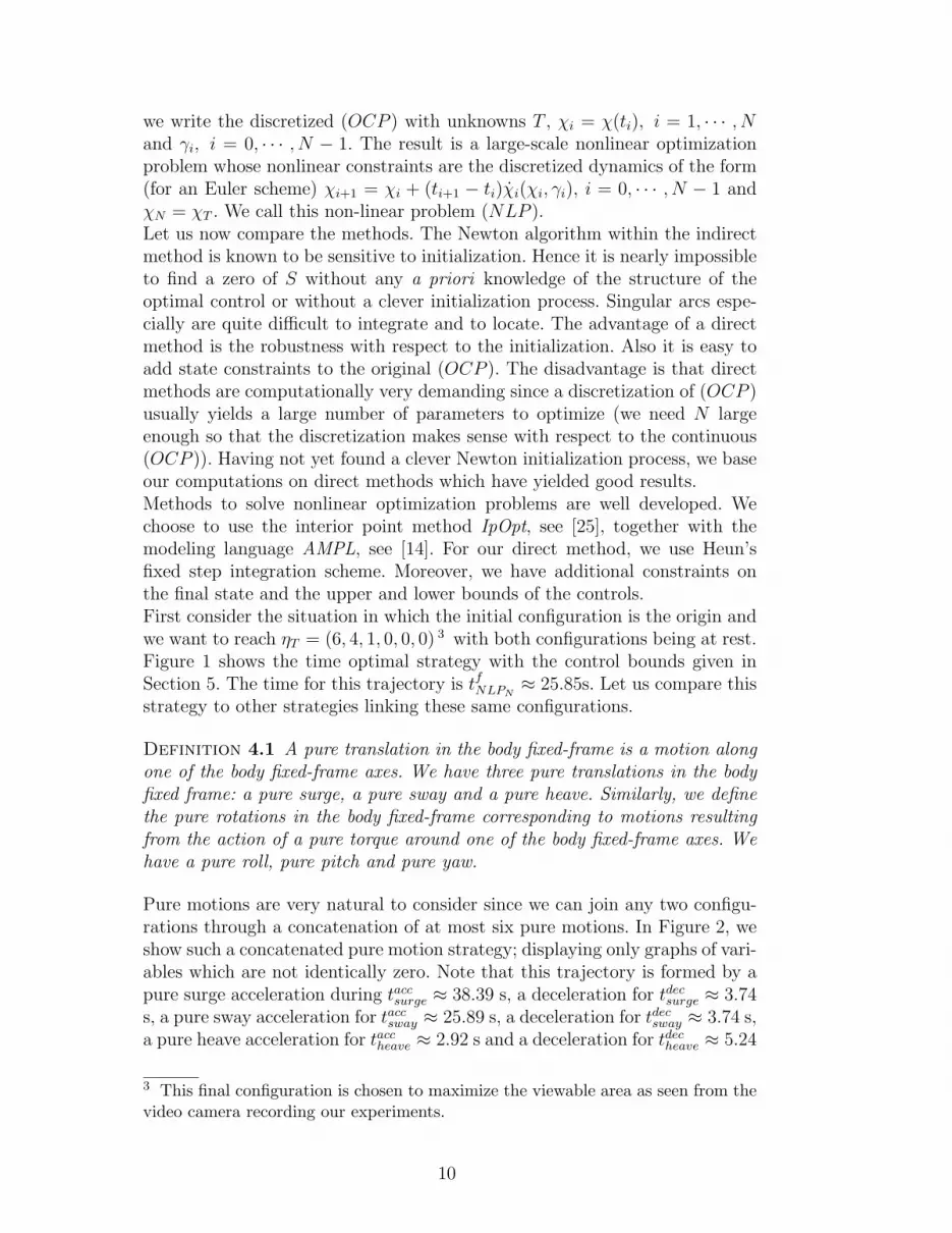
we write the discretized (OCP ) with unknowns T , χi = χ(ti), i = 1, · · · , Nand γi, i = 0, · · · , N − 1. The result is a large-scale nonlinear optimizationproblem whose nonlinear constraints are the discretized dynamics of the form(for an Euler scheme) χi+1 = χi + (ti+1 − ti)χi(χi, γi), i = 0, · · · , N − 1 andχN = χT . We call this non-linear problem (NLP ).Let us now compare the methods. The Newton algorithm within the indirectmethod is known to be sensitive to initialization. Hence it is nearly impossibleto find a zero of S without any a priori knowledge of the structure of theoptimal control or without a clever initialization process. Singular arcs espe-cially are quite difficult to integrate and to locate. The advantage of a directmethod is the robustness with respect to the initialization. Also it is easy toadd state constraints to the original (OCP ). The disadvantage is that directmethods are computationally very demanding since a discretization of (OCP )usually yields a large number of parameters to optimize (we need N largeenough so that the discretization makes sense with respect to the continuous(OCP )). Having not yet found a clever Newton initialization process, we baseour computations on direct methods which have yielded good results.Methods to solve nonlinear optimization problems are well developed. Wechoose to use the interior point method IpOpt, see [25], together with themodeling language AMPL, see [14]. For our direct method, we use Heun’sfixed step integration scheme. Moreover, we have additional constraints onthe final state and the upper and lower bounds of the controls.First consider the situation in which the initial configuration is the origin andwe want to reach ηT = (6, 4, 1, 0, 0, 0) 3 with both configurations being at rest.Figure 1 shows the time optimal strategy with the control bounds given inSection 5. The time for this trajectory is tfNLPN

≈ 25.85s. Let us compare thisstrategy to other strategies linking these same configurations.

Definition 4.1 A pure translation in the body fixed-frame is a motion alongone of the body fixed-frame axes. We have three pure translations in the bodyfixed frame: a pure surge, a pure sway and a pure heave. Similarly, we definethe pure rotations in the body fixed-frame corresponding to motions resultingfrom the action of a pure torque around one of the body fixed-frame axes. Wehave a pure roll, pure pitch and pure yaw.

Pure motions are very natural to consider since we can join any two configu-rations through a concatenation of at most six pure motions. In Figure 2, weshow such a concatenated pure motion strategy; displaying only graphs of vari-ables which are not identically zero. Note that this trajectory is formed by apure surge acceleration during tacc

surge ≈ 38.39 s, a deceleration for tdecsurge ≈ 3.74

s, a pure sway acceleration for taccsway ≈ 25.89 s, a deceleration for tdec

sway ≈ 3.74 s,a pure heave acceleration for tacc

heave ≈ 2.92 s and a deceleration for tdecheave ≈ 5.24

3 This final configuration is chosen to maximize the viewable area as seen from thevideo camera recording our experiments.

10

0 10 20−10

0

10

γ ν 1

0 10 20−10

0

10

γ ν 2

0 10 20−20

0

20

40

γ ν 3

t (s)

0 10 20−5

0

5

γ Ω1

0 10 20−5

0

5

γ Ω2

0 10 20−1

0

1

γ Ω3

t (s)Fig. 1. Time Optimal thrust strategy ending at ηT = (6, 4, 1, 0, 0, 0) at rest.

0 20 40 60−10

0

10

γ ν 1

0 20 40 60−10

0

10

γ ν 2

0 20 40 60−20

0

20

40

γ ν 3

t (s)

0 20 40 600

5

10

b 1

0 20 40 600

2

4

b 2

0 20 40 600

0.5

1

b 3

t (s)Fig. 2. Pure surge, sway and then heave in order to reach ηT = (6, 4, 1, 0, 0, 0) m.

s. The non-symmetry of the acceleration and deceleration phases is due to dragforces and thruster unsymmetries. The total transfer time for this trajectory istpure ≈ 79.92 s. The duration is more than triple the optimal time! This is ac-tually not that surprising since the pure motion trajectory uses only a fractionof the available thrust. A pure motion control strategy is attractive for ourproblem due to its piecewise constant structure but it is far from time efficient.Notice that the same should be true when considering energy consumption.It is inefficient to concatenate motions through configurations at rest. Now

11

back to the time optimal strategy. The structure here is mostly bang-bang,except for the τΩ3 control which contains singular arcs. These singular arcsdepend on our choice of initial and final configurations. Orienting the vehi-cle correctly allows it to use the full power of the translational controls, butit needs to maintain this orientation over the entire trajectory. Singular arcsdo not appear in τΩ1 and τΩ2 because their full power is needed to offset therestoring moments. The translational controls ϕν1,ν2,ν3 are used to their fullextent, as one would expect for a time optimal translational displacement.Other than the τΩ3 singular arc, the time optimal control strategy has anothersevere drawback when considering practical implementation. From Figure 1,we can count 21 actuator switching times. Each switching generates errorssince the physical thrusters have an unstable behavior for abrupt changes ofdirection. We cannot match the accuracy of the solution with the refresh rateon a real vessel because it would require storage of impractical amounts ofdata. From a computational point of view, obtaining the time optimal tra-jectory is time consuming and data storage limiting. To accurately track thesingular arcs and handle the large number of switches, one solution similar tothat represented in Figure 1 requires about 15 minutes of computation.From the above remarks, neither a control strategy based on pure motions norone based on time optimal trajectories alone is a viable option for practicalimplementation onto a test-bed vehicle. The next section takes the advan-tages of both control strategies and combines them to create the new hybridmethod.

4.2 Switching time parameterization algorithm

Inspired from the work in [15,23], we developed another approach to over-come the issues seen in the previous solving methods. In [23], the authors usethe discretized solution of an optimal control problem to extract the switch-ing structure of the optimal control. Then, they rewrite the optimal controlproblem as a nonlinear optimization problem whose unknowns are the switch-ing times (more precisely the time length between two switches). A high orderintegrator can be used to integrate the obtained dynamic system. The motiva-tion for their approach is the verification of second order sufficient conditionsfor optimality. Along singular trajectories they are allowed to write the controlas a feedback both the state and adjoint variables. This can not be done inour situation. In [6] we detail the computations for the singular components ofthe control. The formulas for the singular components are very complex andthe feedback depends on the adjoint variables. Moreover, the structure of theoptimal solution is very difficult, if not impossible, to extract.It is important to note that our primary goal is to produce a time efficientwhich can be easily implemented onto a test-bed vehicle. By time efficient, wemean that the trajectory duration is close in time to that of the time optimal

12

solution. To this end, we first note that a translational displacement can al-ways be achieved by a thrust strategy with a single switching time at whichthe 3 components of ϕν change. We extend this idea by imposing the structureof the control strategy but not basing it on the solution of the (NLP ) prob-lem. We fix the number of switching times along the trajectory, preferably toa small number, and we numerically determine the optimal trajectory fromthese candidates. We call this new optimization problem (STPP )p (SwitchingTime Parameterization Problem) where p refers to the number of switchingtimes. The unknowns are the time periods between two switching times alongwith the time period between the last switch and the final time, and the val-ues of the constant thrust arcs. It is essential for convergence that the latervalues are introduced as parameters. Our construction does not necessarilyproduce bang-bang trajectories. The new optimization problem (STPP )p hasthe following form:

(STPP )p

minz∈D

tp+1

t0 = 0

ti+1 = ti + ξi , i = 1, · · · , p

χi+1 = χi +∫ ti+1ti χ(t, γi)dt

χp+1 = χT

z = (ξ1, · · · , ξp+1, γ1, · · · , γp+1)

D = IR(p+1)+ × Up+1

(25)

where ξi, i = 1, · · · , p+1 are the time arclengths and γi ∈ U , i = 1, · · · , p+1are the values of the constant thrust arcs. The right hand side of the dynamicsystem defined by (7)-(18) is simply χ(t, γi), with the constant control γi.To integrate the dynamic system of (STPP )p we use DOP853, a high orderadaptative step integrator [16]. This allows us to minimize potential differencesbetween the theoretical computations and the experiments. Uncertainties arealready introduced with the approximated model. Compared to the compu-tation time of the solutions of (NLP ), we gain considerable computationaltime with our (STPP )p procedure. The reason is the drastic reduction in thenumber of unknowns. Even though the integration takes more time, the com-putational resources needed to solve (STPP )p are drastically reduced. Notethat (STPP )p is another way to discretize the (OCP ) which could be calleda variable step recursive discretization. Variable step implies the arclength be-tween two discretization times is an optimization parameter. Recursive impliesthat the control is an optimization parameter and the final value of the stateis computed recursively from the initial to the final time. If N is large enough(to insure convergence for (NLP )), the solutions of (STPP )N−1 are better

13

than the solutions of (NLP )N . Clearly, the following inequalities are true:

tfmin ≤ tfSTPPp+1≤ tfSTPPp

≤ tfNLPp(26)

where tfNLPpis the time of the solution of (NLP ) with p discretization points,

and tfmin is the theoretical minimum time. However, we are interested in solu-tion of (STPP )p when p is small.In Figures 3 and 4, we compare the solution of (NLP ) for the initial and finalconfigurations used in Section 4.1 with the solution of (STPP )4 for the sameset of configurations. Notice that the final time tfSTPP4

is less than 6% more

0 5 10 15 20 25−10

0

10

γ ν 1

0 5 10 15 20 25−10

0

10

γ ν 2

0 5 10 15 20 25−20

0

20

40

γ ν 3

t (s)

0 5 10 15 20 25−5

0

5

γ Ω1

0 5 10 15 20 25−5

0

5

γ Ω2

0 5 10 15 20 25−1

0

1

γ Ω3

t (s)Fig. 3. Control strategy solution of (NLP ) (N = 1000, tfNLP ≈ 26.58 s, solid line)and of (STPP )4 (tfSTPP 4

≈ 28.02 s, dashed line).

than the time optimal trajectory. Through many experiments, we have shownthat the trajectory time computed using the switching times parameterizationalgorithm is within 10% of the optimal trajectory time. An open question isa formal proof of this result. With our new algorithm we produce not onlytrajectories that are easily implementable and time efficient but we also dra-matically reduced the computational time. Solving (STPP )p takes less than30 s on the same platform which earlier quoted 15 minutes to solve (NLP ).The simulations show a sensitivity in the initialization process of our switch-ing time parameterization algorithm and that there are few local minima. TheSTPP strategy is easier to implement than the (NLP ) because of the reducednumber of switching times and the piecewise constant property. As seen in thegraphs, the control strategies of (NLP ) and (STPP )4 share some properties.This suggests the use of (STPP )p solutions as an initialization point to the(NLP ). However, simulations have shown that the time gained using such aprocedure is not substantial, and we still have the problem of the singulararcs.

14

From the two control strategies seen in Figure 3, we display the correspondingtheoretical trajectories in Figure 4. The two trajectories are very similar. For

0 5 10 15 20 250

2

4

6

b 1

0 5 10 15 20 250

2

4

b 2

0 5 10 15 20 25−1

0

1

2

b 3

t (s)

0 5 10 15 20 25−0.5

0

0.5

φ

0 5 10 15 20 25−0.5

0

0.5

1

θ

0 5 10 15 20 25−0.5

0

0.5

ψ

t (s)Fig. 4. Trajectory solution of (NLP ) (N = 1000, tfNLP ≈ 26.58 s, solid line) and of(STPP )4 (tfSTPP 4

≈ 28.02 s, dashed line).

the optimal trajectory (solid line), the evolution of ψ, during the singular arc,is constant. Whereas for the (STPP )4 solution (dashed line), ψ is slightlyevolving over the entire trajectory. In Table 1 we analyze tfSTPPp

for differentp and alternate final configurations. The initial configuration is always η0 = 0and ν0 = Ω0 = 0. Because of instant control (thruster) switches, the reader

Final (NLP ) (STPP )p

Configuration tfNLP # sw. Singular? tfSTPP2tfSTPP3

tfSTPP4

(6, 4, 1, 0, 0, 0) 26.58 s 21 Yes 28.72 s 28.10 s 28.02 s

(6, 4, 0, 0, 0, 0) 28.42 s 28 Yes 34.43 s 29.83 s 29.01 s

(6, 0, 0, 0, 0, 0) 25.40 s 23 Yes 31.52 s 28.45 s 26.55 s

(0, 6, 0, 0.2, 0.3, 0) 25.46 s 19 Yes 30.09 s 29.05 s 28.98 sTable 1Final times for different final configurations (#sw. = number of switchings)

may be surprised that piecewise constant control strategies are easily imple-mentable on a test-bed vehicle. We remedied this by connecting the piecewiseconstant arcs by a linear function which ramps the control from max to min orvise versa. This linear function is chosen in such a way that its slope does notdamage the AUV’s electronics (i.e. vehicle specific). The vehicle used in theexperiments has an internal refresh rate R = 33 Hz. Actuator switchings gen-erally occur over a period of a few R intervals. We also implemented electronicsafety circuits to control any induced voltage or current.

15

5 Experiments

5.1 Test-Bed AUV

The test-bed AUV we use is the Omni-Directional Intelligent Navigator (ODIN)which is owned and operated by the Autonomous Systems Laboratory (ASL),College of Engineering at the University of Hawaii. The experiments conductedfor this research are carried out at the Duke Kahanamoku Swimming Com-plex at the University of Hawaii. As seen in Figure 5, ODIN has a spherical

Fig. 5. ODIN operating in the pool.

hull which is 65cm in diameter. This sphere is constructed from an aluminumalloy to prevent corrosion. Eight thrusters are attached to the sphere via fourfabricated mounts, each holding two thrusters. The thrusters are evenly dis-tributed around the sphere with four vertical and four horizontal. Fully assem-bled, ODIN weighs 126.55kg and is positively buoyant by ≈ 0.1kg. ODIN iscapable of moving in six DOF from either a remote or autonomous mode. Forour experiments, ODIN is tethered, but only to send commands via TCP/IPprotocol from a shore based laptop to be run in autonomous mode. This setupallows for multiple tests to be conducted without removing ODIN from the wa-ter to upload mission sorties. ODIN’s internal CPU is a 800 MHz Intel basedprocessor running on a PC104+ form factor with two external I/O boardsproviding A/D and D/A operations. Major internal components include apressure sensor, inertial measurement unit (IMU) and 24 batteries. ODIN iscapable of computing real time, yaw, pitch, tilt, and depth and can run au-tonomously for up to 5 hours. However the IMU is not designed to track fastchanges of heading (≥ 6/s). The software is divided into two components.The first component is based on a real time extension to the Windows 2000operating system, which provides ODIN real time autonomous control. Thesecond component runs on the remote laptop and allows the operator to uploadautonomous mission profiles to ODIN on the fly during testing as well as mon-

16

itor ODIN in real time. As noted above, ODIN does not have real time sensorsto detect horizontal (x, y) position. Instead, experiments are video taped fromthe 10m diving platform, giving us a near nadir view of ODIN’s movements.Videos are saved and horizontal position is post processed for later analysis.A real time system utilizing sonar was available on ODIN, but was abandonedfor two main reasons. First, the sonar created too much noise in the diving wellwhich led to inaccuracies. More significantly, in the implementation of our ef-ficient trajectories, ODIN is often required to achieve large (> 15) list angleswhich render the sonars useless for horizontal position. Many solutions wereattempted and video led to the most accurate results. The numerical valuesof the various parameters used for our theoretical model are given in Table 2.These values were derived from experiments performed on ODIN. The addedmass and drag terms were estimated from formulas found in [19,21]. Momentsof inertia were calculated using experiments outlined in [20]. We used inclin-ing experiments to locate and place CB while we assume that CG is locatedat the center of our body-fixed axis. The drag and CB estimates were thenadapted to match the experimental behavior of the vehicle. Unique to ODIN’s

m 126.55 kg ρg∇ 1241.2 N CB (0.9, 0.2,−7) mm

Muf 70 kg Mv

f 70 kg Mwf 70 kg

Ix 5.46 kg.m2 Iy 5.29 kg.m2 Iz 5.72 kg.m2

Jpf 0 kg.m2 Jq

f 0 kg.m2 Jrf 0 kg.m2

D11ν −27.03 D21

ν −27.03 D31ν −27.03

D12ν −897.66 D22

ν −897.66 D32ν −897.66

D11Ω −13.79 D21

Ω −13.79 D31Ω −11.94

D12Ω −6.46 D22

Ω −6.46 D32Ω −6.94

Table 2Numerical values used for our hydrodynamic model.

construction is the control from an eight dimensional thrust to move in sixDOF. This construction puts redundancy into the system in case of thrusterfailure. It is important to distinguish between a control for the real vehicle,namely the applied control referring to the action of the thrusters, and the sixDOF control introduced previously. Our input trajectories to ODIN take theform of the six DOF controls which are converted onboard ODIN to the con-trol for the eight actual thrusters using the following Thrust Control Matrices(TCM’s) (Eqns. 27 and 28).

TCM horizontal =

−0.707 0.707 0.707 −0.707

0.707 0.707 −0.707 −0.707

0.48160 −0.48160 0.48160 −0.48160

(27)

17

TCM vertical =

−1.0 −1.0 −1.0 −1.0

−0.26989 −0.26989 0.26989 0.26989

0.26989 −0.26989 −0.26989 0.26989

(28)

These transformations are based on the following assumptions. Let us denoteγh

i , i = 1, · · · , 4 as the thrusts induced by the horizontal thrusters and γvi , i =

1, · · · , 4 the thrusts induced by the vertical thrusters. The first assumption isthat points of application of the thrusts γ

(h,v)i lie in a plane going through the

center of the vehicle. We also assume that the distance from the center of thebody frame (CG in our case) to the center of the sphere (CB in our case) is smallwith respect to the radius of the sphere. As a consequence we can decouplethe action of the thrusters as follows. The horizontal thrusters contributeonly to the forces ϕν1 (surge) and ϕν2 (sway) and to the torque τΩ3 (yaw).The vertical thrusters contribute only to the force ϕΩ3 (heave) and to thetorques τν1 (roll) and τν2 (pitch). We have (ϕν1 , ϕν2 , τΩ3)

t = TCM horizontal ·(γh)t and (ϕν3 , τΩ1 , τΩ2)

t = TCM vertical · (γv)t. Assuming that the thrusters

are independently powered, we can reasonably state that each thrust γ(h,v)i is

bounded by fixed values:

γ(h,v) ∈ Υ = γ ∈ IR8|γ(h,v),mini ≤ γ

(h,v)i ≤ γ

(h,v),maxi , i = 1, · · · , 4 (29)

The image of Υ through the above linear transformation is composed of twoflat ellipsoids. We choose a box included within these ellipsoids as domainof control for the six DOF control. There are different possible choices forthis box depending on the controllability properties that we prefer for ourvehicle. In the sequel, we assume the control domain for the component ϕν

and τΩ to be as in Equation (19). For our numerical computations, we willtake αmax

ν1,2= −αmin

ν1,2= 8 N, αmax

ν3= 25 N, αmin

ν3= −5 N, αmax

Ω1,2= −αmin

Ω1,2= 3

N.m and αmaxΩ3

= −αminΩ3

= 1 N.m. The non-symmetry of αmin,maxν3

is due to thefact that the 4 vertical thrusters are all oriented in the same direction. Alongwith the tests to determine the values in Table 2, we also tested the thrusters.Each thruster has a unique voltage input to power output relationship. Thisrelationship is highly nonlinear and is approximated using a piecewise linearfunction which we refer to as our thruster model.

5.2 One Switching STTP Experiment

We begin by testing a (STPP )1 strategy from the origin to ηT = (6, 4, 1, 0, 0, 0).This control strategy contains only one switch and thus does not change theorientation of the vehicle during the motion. This aids the practical implemen-tation since we can apply roll, pitch and yaw feedback stabilization during theexperiment. The only open loop controls are the translational ϕν1 , ϕν2 andϕν3 . Here the linear function connecting the constant thrust arcs occur over

18

a duration of 0.9 s. This linear function minimally increases the total timewhen compared to the purely piecewise constant (STPP ) strategy. Figure 6displays the applied translational controls. The evolution of ODIN’s positionduring the experiment is given by the solid line and the prescribed evolution(theoretical evolution we wanted to achieve) is given by the dashed line. Notethat, from the point of view of this paper, there is no need to display the orien-tation evolution or the angular control since they are computed in closed-loopwith feedback and we are not interested in the efficiency of the feedback con-troller. The total time of this strategy is tfSTPP1

≈ 42.55 s which is actually the

0 10 20 30 40

−5

0

5

γ ν 1 (N

)

0 10 20 30 40−6

−4

−2

0

2

4

γ ν 2 (N

)

0 10 20 30 40−1

0

1

2

3

γ ν 3 (N

)

t (s)

0 10 20 30 400

2

4

6

b 1 (m

)

0 10 20 30 400

1

2

3

4

5

b 2 (m

)

0 10 20 30 400.5

1

1.5

2

2.5

b 1 (m

)

t (s)

Fig. 6. Experimental (solid) and prescribed (dashed) evolutions of the AUV for a(STPP )1 strategy ending at ηT = (6, 4, 1, 0, 0, 0).

time needed to do just a pure surge motion of 6 m with the prescribed linearjunction. This duration is not surprising at all since the (STPP )1 method issimply a modified pure motion. Here the direction of the motion is not alongone of the body fixed axes, but along a line in the direction from the initialto the final configuration. A (STPP )1 strategy takes as long as the longestpure motion of a pure motion strategy. The evolutions of b1 and b2 exactlycorrespond to surge and sway since there is no orientation alteration. We seethat the experimental is very close to the prescribed path. This indicates thatour drag and thrust magnitudes are well estimated. We found similar behaviorover various thrust magnitudes implying that our thrust and drag coefficientestimates are consistent. The behavior of b3 (heave) is slightly more erraticand deviant than b1 and b2. This behavior is a result of noise within the depthsensor circuitry and buoyancy effects from the tether. Since ODIN is nearneutrally buoyant, small buoyancy alterations have noticeable effects. Thisexperiment validates part of our hydrodynamic model and thruster calibra-tion. This gives very promising results even though the (STPP )1 strategy isnot exceptionally time efficient.

19

5.3 Two Switchings STPP Experiment

Building on the good results from Section 5.2, we now consider a (STPP )2

strategy with the same final configuration. This trajectory contains a large listangle. This makes orientation tracking nearly impossible due to the poor dy-namic behavior of our sensors (especially for ψ). Including the linear junction,the total duration of this trajectory is tfSTPP2

≈ 28.66 s. This experiment doesnot use any feedback control. The results test and help update the accuracy ofour hydrodynamic model as well as our thruster calibration. In Figure 7, weshow the control strategy applied during the experiment. The (STTP )1 strat-

0 5 10 15 20 25

−5

0

5

γ ν 1 (N

)

0 5 10 15 20 25

−5

0

5

γ ν 2 (N

)

0 5 10 15 20 25

0

10

20

γ ν 3 (N

)

t (s)

0 5 10 15 20 25

−3

−2

−1

0

γ Ω1 (

N)

0 5 10 15 20 25−1

0

1

2

3

γ Ω2 (

N)

0 5 10 15 20 25−0.4

−0.2

0

0.2

0.4

γ Ω3 (

N)

t (s)

Fig. 7. (STPP )2 control strategy targeting ηT = (6, 4, 1, 0, 0, 0).

egy maximized only one control whereas here, the (STPP )2 strategy usedfour of the controls to their maximum extent (γν1 , γν2 , γΩ1 and γΩ2). Thistrajectory requires ODIN to realize a list of about 60. Due to compensationfor the restoring moments in pitch and roll, we can not maximize the heavecontrol over the trajectory. And, in yaw there is never any significant forceto overcome, thus it will never show a maximized control output. Overall, wenote that this (STPP )2 strategy resembles the pure motion control strategyshown earlier. In Figure 8 we display the experimental and theoretical evolu-tion of the vehicle. We modify the theoretical evolution by an initial rotationto match the orientation ODIN started with in the pool. Before analyzing thisexperimental result, we would like emphasize again that we are completely inan open loop framework. All controls are computed before the experiment.First note that the evolution of the yaw does not match the prescribed strat-egy. This is nearly impossible to fix it since there are minimal restoring forcesacting in this direction. Any misappropriated thrust will result in a parasiteyaw torque. This significantly affects the yaw evolution since there is nothingto counter act it. Parasite torques exist for roll and pitch but are far less prob-

20

0 5 10 15 20 250

2

4

6

b 1 (m

)

0 5 10 15 20 250

1

2

3

4b 2 (

m)

0 5 10 15 20 25

1

2

3

4

b 3 (m

)

t (s)

0 5 10 15 20 25−40

−20

0

20

φ (d

eg)

0 5 10 15 20 25−50

0

50

θ (d

eg)

0 5 10 15 20 25−100

−50

0

50

ψ (

deg)

t (s)

Fig. 8. Experimental (solid) and theoretical (dashed) evolutions of the AUV for the(STPP )2 strategy ending at ηT = (6, 4, 1, 0, 0, 0).

lematic. The restoring moments make any parasite torques nearly negligible.Speaking of the evolution of φ and θ, we see that the general trend of the pre-scribed motion is respected up to the transient behavior. During the transientbehavior we can notice rather important overshooting that have three mainreasons. The first reason is the overshooting of the thrusters. This indicatesthat our 0.9 s linear junction still does not erase the transient response ofthe thrusters. However, using a larger duration for the junction would renderthe (STPP )p control strategy less time efficient and might even impair itsconvergence. The second identified reason is the sensor accuracy and tran-sient behavior. As for the yaw, we cannot rule out that the sensor are proneto misreading when confronted to fast change of orientation. A final reasonwould be an over estimation of the drag coefficient in pitch and roll (and thenin yaw by symmetry). Indeed the observed overshooting looks very similar towhat would happen to a less damped system. Future experiments will try todetermine the respective impact of those three issues and to cope with them.The depth evolution (b3) looks fine until about 20 s when ODIN dove morethan expected. This is caused by the instability of the thrusters around aswitching along with some overshooting based on inaccurate drag estimates.We are also examining the effect of the tether on the buoyancy of ODIN. Forthe horizontal motions, we note a good comparison in surge, while the swayevolution leaves much to be desired. However, with the overshooting issue inpitch and roll, we can not expect to match both surge and sway evolutionswith the prescribed motion. For the (STPP )2 trajectory, we have found thatthe drag of the tether may not be small as first expected.

21

6 Conclusion

Bridging the gap between theory and application is the ultimate goal of controltheory. During the past two decades, major developments have occurred in thefield of geometric control. The work presented here is based on recent progressmade in geometric optimal control with the objective to develop an efficienttool for scientists such as oceanographers. Our underwater vehicle applicationsuccessfully demonstrates the applicability of these geometric methods to de-sign trajectories for a concrete applications. In the reverse, the underwatervehicles presents an ideal platform to extend the theory to mechanical sys-tems with dissipative and potential forces. In particular, we are interested inthe extension of the notion of kinematic reductions. For the next step, we arecurrently studying the addition of energy consumption as a minimization cost.Since we can determine the optimal time between two configurations at rest,we can consider the trade-off between energy consumption and duration ofthe trajectory. Trajectories which minimize energy consumption can be com-puted using similar numerical techniques as presented for time minimization inthis paper. Moreover, implementation will be straightforward since the controlstrategy design is the same.

Acknowledgment

We would like to take time to thank a few people without whom this researchwould not succeed. We thank Bruce Kennard, the UH pool coordinator, for hisongoing flexibility and willingness to fit us into an already busy schedule. ChrisMcLeod has been beneficial to the project with his knowledge and expertisein electrical engineering and general maintenance and upkeep of ODIN. Also,thank you to Jeff Fines for his devotion to the mundane filming and filmanalysis of all the experiments which we conduct.

References

[1] Volker Bertram and Alberto Alvarez. Hydrodynamic Aspects of AUV Design.5th International Conference on Computer Applications and InformationTechnology in the Maritime Industries Leiden/Netherlands, 2006.

[2] B. Bonnard and M. Chyba. Singular Trajectories and their Role in ControlTheory. Springer-Verlag, 2003.

[3] R.W. Brocket. Minimum Attention Control, In 36th IEEE Conf. on Decisionand Control, San Diego, 1997.

22

[4] R.W. Brocket. Minimum Attention Control in a Motion Control Context, In42th IEEE Conf. on Decision and Control, Maui, 2003.

[5] F. Bullo and A.D. Lewis. Geometric Control of Mechanical Systems Modeling,Analysis, and Design for Simple Mechanical Control Systems. Springer-Verlag,New York-Heidelberg-Berlin, 49 in Texts in Applied Mathematics, 2004.

[6] M.Chyba, T. Haberkorn. R.N. Smith. G.R. Wilkens. Geometric Properties ofSingular Extremals for a Submerged Rigid Body, Preprint, 2007.

[7] M. Chyba, T. Haberkorn, R.N. Smith, Scott Weatherwax and Song K.Choi. ”Experimental Analysis of a Theoretical AUV Model”. Submitted26th International Conference on Offshore Mechanics and Artic Engineering(OMAE), San Diego, 2007.

[8] M. Chyba and T. Haberkorn. “Autonomous Underwater Vehicles: SingularExtremals and Chattering”. Proceedings of the 22nd IFIP TC 7 Conferenceon System Modeling and Optimization, Italy, 18-22 July 2005.

[9] M. Chyba and T. Haberkorn. “Designing Efficient Trajectories for UnderwaterVehicles Using Geometric Control Theory”. Proceedings of the 24rdInternational Conference on Offshore Mechanics and Arctic Engineering,Greece, 12-17 June 2005.

[10] M. Chyba, N.E. Leonard and E.D. Sontag. “Singular Trajectories in the Multi-Input Time-Optimal Problem: Application to Controlled Mechanical Systems”.Journal on Dynamical and Control Systems 9(1):73-88, 2003.

[11] M. Chyba. “Underwater Vehicles: A Surprising Non Time-Optimal Path”.In42th IEEE Conf. on Decision and Control, Maui 2003.

[12] M.Chyba, H. Maurer, H.J. Sussmann and G. Vossen. “Underwater Vehicles: TheMinimum Time Problem”. In Proceedings of the 43th IEEE Conf. on Decisionand Control , Bahamas, 2004.

[13] T.I. Fossen. “Guidance and Control of Ocean Vehicles”. Wiley, New York, 1994

[14] R. Fourer, D.M. Gay and B.W. Kernighan. “AMPL: A Modeling Languagefor Mathematical Programming”. Duxbury Press, Brooks-Cole PublishingCompany,1993.

[15] C.Y. Kaya and J.L. Noakes. “Computation Method for Time-Optimal SwitchingControl”. Journal of Optimization Theory and Applications, 117(1):69-92, 2003.

[16] E. Hairer, S.P. Norsett and G. Wanner.“Solving Ordinary DifferentialEquations I. Nonstiff Problems. 2nd edition”.Springer series in computationalmathematics, Springer Verlag, 1993.

[17] N.E. Leonard. “Stability of a Bottom-Heavy Underwater Vehicle”. Automactica,33(3):331-46, 1997.

[18] N.E. Leonard. Stabilization of Steady Motions of an Underwater Vehicle, Proc.of the 35th IEEE Conference on Decision and Control, 1996.

23

[19] F.H. Imlay. “The Complete Expressions for Added Mass of a Rigid Body Movingin an Ideal Fluid”. Technical Report DTMB, 1961.

[20] R. Bhattacharyya. “Dynamics of Marine Vehicles”, Wiley, 1978.

[21] E. Allmendinger. “Submersible Vehicle Design”, SNAME, 1990.

[22] Malcolm A. MacIver, Ebraheem Fontaine and Joel W. Burdick. “DesigningFuture Underwater Vehicles: Principles and Mechanisms of the Weakly ElectricFish”. In IEEE Journal of Oceanic Engineering , Volume 29, No. 3, July 2004.

[23] H. Maurer, C. Buskens, J-H.R. Kim and I.C. Kaya. “Optimization Methods forNumerical Verification of Second Order Sufficient Conditions for Bang-BangControls”. Optimal Control Application and Methods, 26:129-156, 2005.

[24] Levente Molnar, Edin Omerdic and Daniel Toal. “Hydrodynamic Aspects ofAUV Design”. Ocean 2005 Europe IEEE Conference Brest, France, June 2005.

[25] A. Waechter and L. T. Biegler. “On the Implementation of an Interior-Point Filter-Line Search Algorithm for Large-Scale Nonlinear Programming”.Research Report RC 23149, IBM T.J. Watson Research Center, Yorktown,New-York.

24