http://pic.sagepub.com/Engineering Science

Engineers, Part C: Journal of Mechanical Proceedings of the Institution of Mechanical

http://pic.sagepub.com/content/215/1/27The online version of this article can be found at:

 DOI: 10.1243/0954406011520490

215: 27 2001Proceedings of the Institution of Mechanical Engineers, Part C: Journal of Mechanical Engineering Science

D Akdas and G A Medrano-Cerdaregulator theory

Design of a stabilizing controller for a ten-degree-of-freedom bipedal robot using linear quadratic  

Published by:

http://www.sagepublications.com

On behalf of: 

  Institution of Mechanical Engineers

can be found at:Engineering ScienceProceedings of the Institution of Mechanical Engineers, Part C: Journal of MechanicalAdditional services and information for

   

  http://pic.sagepub.com/cgi/alertsEmail Alerts:

 

http://pic.sagepub.com/subscriptionsSubscriptions:  

http://www.sagepub.com/journalsReprints.navReprints:  

http://www.sagepub.com/journalsPermissions.navPermissions:  

http://pic.sagepub.com/content/215/1/27.refs.htmlCitations:  

What is This? 

- Jan 1, 2001Version of Record >>

at The University of Manchester Library on November 12, 2013pic.sagepub.comDownloaded from at The University of Manchester Library on November 12, 2013pic.sagepub.comDownloaded from

Design of a stabilizing controller for aten-degree-of-freedom bipedal robot usinglinear quadratic regulator theory

D Akdas* and G A Medrano-Cerda

Department of Electronic and Electrical Engineering, University of Salford, UK

Abstract: This paper considers the design and evaluation of stabilizing controllers for a ten-degree-

of-freedom (10 DOF) biped robot using linear quadratic optimal control techniques and reduced-

order observers. The controllers are designed using approximate planar dynamical models for thesagittal and lateral planes. Experiments were carried out to test the control system when the biped

robot was in the double-support phase and the robot was subject to external disturbances. Although

the control system is based on single-support models, the experimental results have shown that the

robot successfully kept its given posture under disturbances.

Keywords: stabilizing controller, bipedal robot, linear quadratic regulator theory

1 INTRODUCTION

In recent years, there has been an increased interest in

bipedal robots. In particular, the creation of the Eur-

opean Network on Climbing and Walking Robots

(CLAWAR) has provided a focus for worldwide

research on mobile robotics. Experimental prototypes

have been developed throughout the world and, atpresent, the most remarkable results have been achieved

by Hirai et al. [1]. However, biped robots are still quite

primitive and a substantial amount of research is needed

to develop a biped capable of performing useful tasks inunstructured and hazardous environments. Some

attractive features of two-legged robots are their

potential to navigate in con® ned spaces, walk on rough

terrain and ascend/descend stairs.

One of the major problems in bipedal robots is that ofpreserving stability during locomotion as well as stati-

cally. This problem alone provides a substantial engi-

neering challenge. Hierarchical control architectures are

usually adopted to achieve stable locomotion, particu-

larly at high speeds. High-level controllers generate

suitable walking patterns according to terrain condi-

tions, speed and gait. The realization of a walking pat-tern is then the task of low-level joint controllers.

Several researchers have investigated stabilization

strategies based on modern control theory and linear-

ized (planar) models. Mita et al. [2] used linear optimal

regulator theory; Eldukhri [3] and Medrano-Cerda and

Eldukhri [4] considered linear optimal control imple-

mented via reduced-order observers. Hemami and

Wyman [5] and Golliday and Hemami [6] used pole

placement controllers in their simulation studies;decoupling control was studied by Raibert [7] and

Golliday and Hemami [8]. Comparative simulation

studies were presented in reference [9] for PD, computed

torque and sliding mode controllers. Miura and Shi-

moyama [10] used linear state feedback to stabilizemotions around carefully preselected trajectories.

An alternative approach is to use low-level servo-

controllers for each joint to track a desired trajectory.

The stabilization is then carried out entirely by high-

level controllers. Channon et al. [11] used local PD joint

controllers with gravity compensation and gain sche-

duling; slow motion stabilization was achieved by con-

trolling the position of the centre of gravity. Inaba et al.

[12] followed a similar approach for static balancing

using vision feedback to control the centre of gravity

position. Strategies using neural networks have been

suggested by Fukuda et al. [13], Kun and Miller [14] and

Salatian and Zheng [15]. For high-speed locomotion, the

problem of maintaining balance involves controlling the

position of the zero moment point (ZMP) [16]. TheZMP method has been frequently used in biped robot

stabilization. For a biped with a trunk, the outline of the

method is as follows [17, 18]:

1. For a chosen terrain, the leg trajectories and desired

ZMP trajectory are speci® ed.

The MS was received on 20 September 1999 and was accepted afterrevision for publication on 21 March 2000.* Corresponding author: Department of Electron and ElectricalEngineering, University of Salford, Salford M5 4WT, UK.

27

C12899 ß IMechE 2001 Proc Instn Mech Engrs Vol 215 Part C at The University of Manchester Library on November 12, 2013pic.sagepub.comDownloaded from

2. The trunk motion stabilizing the robot for the

chosen trajectories is determined.3. The trajectories in 1 and 2 are used as reference

inputs for the local joint servos.

Since the stabilizing trunk motion is computed using

mathematical models, there will be discrepancies

between the desired ZMP and the actual ZMP trajec-tories. For large errors, locomotion stability cannot be

guaranteed. Li et al. [19] considered using measure-

ments of the actual ZMP to modify the trunk motion

so that ZMP errors become small. Re® nements and

variations to the basic ZMP approach have been

investigated in recent years. Yamaguchi et al. [20] useda three degree-of-freedom (3 DOF) trunk to stabilize a

biped robot. An adaptive controller that modi® es the

initial leg trajectories using information about the foot

landing surface was proposed by Yamaguchi et al. [21].

The ZMP approach has also been extended to bipedrobots with arms. [22] The humanoid robot developed

by Hirai et al. [1] is also based on the ZMP method,

but a slightly diŒerent scheme to the one described

above is used. The authors claim that their posture-

stabilizing controller is similar to that of humans, yetwhen walking or standing on ¯ at surfaces the angles in

the sagittal plane are rather large. This is particularly

noticeable in the knee joints. The magnitudes of these

angles could be reduced by specifying a slightly

diŒerent walking pattern. For small sagittal angles the

eŒects of backlash can become a problem, but a suit-

ably designed joint control system should overcome

this di� culty. It is believed that the performance of local

PD joint controllers can be greatly improved by more

sophisticated low-level controllers (see also reference

[9]). In previous research [3, 4] the present authors have

designed and tested joint controllers for locomotion in

the sagittal plane on ¯ at surfaces. Results showed that

during the single-support phase the leg joints could be

straightened and, while standing on both feet, small

angles could be maintained to reduce power consump-

tion. The ® rst prototype had eight degrees of freedom,

seven in the sagittal plane and one in the lateral plane

(trunk). This joint distribution limited the robot loco-

motion to the sagittal plane. Additional degrees of

freedom were needed for locomotion in the lateral plane.

Therefore, two more degrees of freedom have been

inserted in the lateral plane. The work in this paper is an

extension of previous research to include multiple

degrees of freedom in both sagittal and lateral planes.

To simplify the design, independent stabilizing con-

trollers are developed for the sagittal and lateral planes.

A brief description of the new biped robot is given in

Section 2. The technique used for derivation of mathe-

matical models and the designs of the control systems

are presented in Section 3. The robustness and dis-

turbance transmission properties of the control systems

are assessed in Section 4. Experimental results are given

in Section 5. Conclusions and further work are sum-

marized in Section 6.

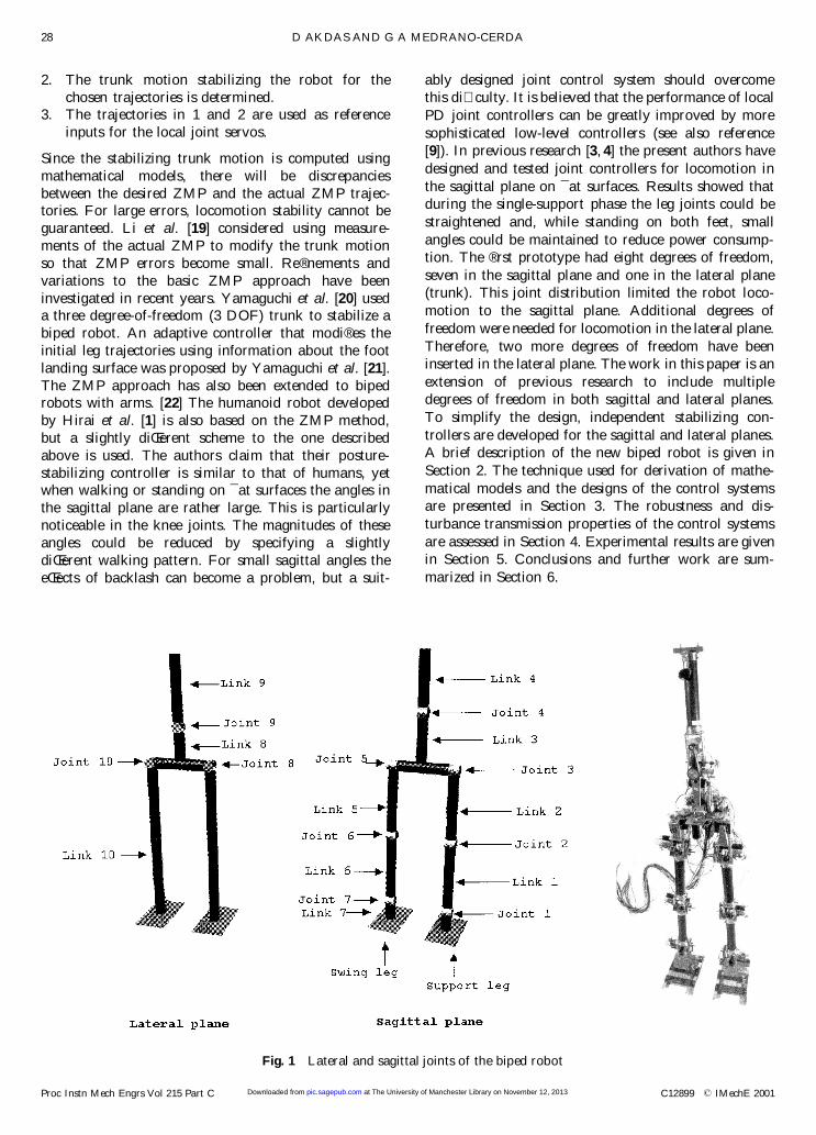
Fig. 1 Lateral and sagittal joints of the biped robot

28 D AKDAS AND G A MEDRANO-CERDA

Proc Instn Mech Engrs Vol 215 Part C C12899 ß IMechE 2001 at The University of Manchester Library on November 12, 2013pic.sagepub.comDownloaded from

2 SYSTEM DESCRIPTION

The new bipedal robot has ten degrees of freedom, threeof them in the lateral plane and seven in the sagittal

plane. Figure 1 shows the joint distribution. The joints

are driven by permanent magnet d.c. motors and higher-

quality gearboxes (higher e� ciency and smaller back-

lash). Potentiometers are used to measure the relative

joint angles. The robot weighs about 13 kg and is 160 cm

tall. The foot size is 12 cm by 22 cm. The biped is con-trolled by a 486DX20 PC. Smoothing and anti-aliasing

® lters (at 15 and 22 Hz respectively) are used to condi-

tion the signals. The new robot is the second-generation

bipedal robot built at the University of Salford. Themajor modi® cations that were carried out to the ® rst

prototype are:

1. Two hip joints were added in the lateral plane. Both

joints are driven by 90 W d.c. motors and worm-

wheel gearboxes with low backlash (less than

0.02 rad). This has increased the mass of the hipby approximately 3 kg.

2. The trunk gearboxes were replaced with worm-

wheel gearboxes (low backlash). Also, 70 W d.c.

motors are used in the new trunk drives.3. The drives for the knee and hip joints in the sagittal

plane were changed. The new drives use 20 W d.c.

motors. The new gearboxes have larger reduction

ratios than those used in the ® rst prototype [3, 4].

These changes have increased the overall gain of the

drive as well as the contributions of motor inertia

and damping re¯ ected at the output shaft.

Parameter values for the new robot are included in the

Appendix.

3 MATHEMATICAL MODELLING AND

CONTROL SYSTEM DESIGN

Symbolic mathematical models of the biped are

obtained for the sagittal and lateral planes separately. In

this way, the complexity of the symbolic model is

reduced. Kane’s equations of motion have been used to

obtain the corresponding dynamic models assuming anopen-chain structure and that the robot is in the single-

support phase [23]. It is also assumed that the support

foot is in ® rm contact with the ground and slippage does

not occur. Reduced-order models for the double-

support phase (closed-chain structure) are derived byincluding the forces of constraint in the dynamic equa-

tions [5, 23, 24]. In this paper, stabilizing control systems

are designed using linearized single-support models.

However, the control systems should be su� ciently

robust to stabilize linearized models in the double-sup-port phase.

3.1 Mathematical model for the sagittal plane

The general form of the equation for a multi-body sys-

tem is

A ³… † �³ ‡ B ³; _³ _³ ˆ f ‡ CT…³†K

W…³† ˆ 0

…1†

where A and B are n £ n matrices, A…³† is the inertia

tensor matrix, B…³; _³ † _³ is the vector of centripetal and

Coriolis forces. The r £ 1 vector W…³† denotes holo-

nomic constraints and C…³† ˆ @W=@³ is an r £ n matrix

[the Jacobian of W…³†Š, f is an n £ 1 generalized force

vector including eŒects of gravity and input forces andK is an r £ 1 vector denoting forces of constraint. In the

sagittal plane, n ˆ 7 (the number of degrees of freedom)

and r ˆ 2; ³, _³ and �³ denote the relative joint angles,

relative angular velocities and accelerations respec-

tively.

When the biped is in the single-support phase, K ˆ 0.Linearizing (1) around the upright position …³ ˆ _³ ˆ 0†yields a 14-dimensional linear state-space model. This

model, including d.c. motors and gearboxes, can be

written in terms of the state variables of the ® rst six linksand the states of the seventh link (see Fig. 1) as

_x6 ˆ A6x6 ‡ B6u6 ‡ A67x7 ‡ B6

7u7

_x7 ˆ A7x7 ‡ B7u7 ‡ A76x6 ‡ B7

6u6

Taking norms gives

_x6k k4 A6k k x6k k ‡ B6k k u6k k ‡ A67 x7k k ‡ B6

7 u7k k

_x7k k4 A7k k x7k k ‡ B7k k u7k k ‡ A76 x6k k ‡ B7

6 u6k k

where

A6k k ˆ 250:33; B6k k ˆ 22:19

A67 ˆ 18:94; B6

7 ˆ 1:91

A7k k ˆ 202:96; B7k k ˆ 20:42

A76 ˆ 54:31; B7

6 ˆ 2:66

The above results indicate that the contributions of x7

and u7 (the ankle joint) to _x6 are not too large. There-

fore, in order to reduce complexity in the calculations of

the controller, this joint is neglected in the derivation of

the mathematical model in the sagittal plane. However,

the mass of the swing-leg foot is added to the mass of thecorresponding knee link. To keep the swing-leg foot

DESIGN FOR A STABILIZING CONTROLLER FOR A 10 DOF BIPEDAL ROBOT 29

C12899 ß IMechE 2001 Proc Instn Mech Engrs Vol 215 Part C at The University of Manchester Library on November 12, 2013pic.sagepub.comDownloaded from

parallel to the ground, a separate foot controller has

been designed.Neglecting the ankle joint, there are six degrees of

freedom (i.e. n ˆ 6). Linearizing (1) around the upright

position and using a 10 ms sampling time interval, a

linear discrete time model is obtained in state-space

form:

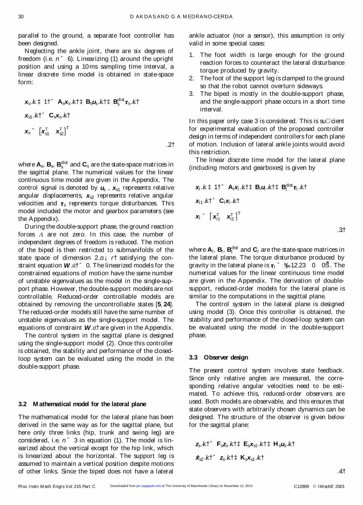
xs…k ‡ 1† ˆ Asxs…k† ‡ Bsus…k† ‡ Bdists ½½½½½s…k†

xs1…k† ˆ Csxs…k†

xs ˆ xTs1 xT

s2

T

…2†

where As, Bs, Bdists and Cs are the state-space matrices in

the sagittal plane. The numerical values for the linearcontinuous time model are given in the Appendix. The

control signal is denoted by us , xs1 represents relative

angular displacements, xs2 represents relative angular

velocities and ½½½½½s represents torque disturbances. This

model included the motor and gearbox parameters (see

the Appendix).During the double-support phase, the ground reaction

forces ¤ are not zero. In this case, the number of

independent degrees of freedom is reduced. The motion

of the biped is then restricted to submanifolds of the

state space of dimension 2…n ¡ r† satisfying the con-straint equation W…³† ˆ 0. The linearized models for the

constrained equations of motion have the same number

of unstable eigenvalues as the model in the single-sup-

port phase. However, the double-support models are not

controllable. Reduced-order controllable models areobtained by removing the uncontrollable states [5, 24].

The reduced-order models still have the same number of

unstable eigenvalues as the single-support model. The

equations of constraint W…³† are given in the Appendix.

The control system in the sagittal plane is designed

using the single-support model (2). Once this controlleris obtained, the stability and performance of the closed-

loop system can be evaluated using the model in the

double-support phase.

3.2 Mathematical model for the lateral plane

The mathematical model for the lateral plane has been

derived in the same way as for the sagittal plane, buthere only three links (hip, trunk and swing leg) are

considered, i.e. n ˆ 3 in equation (1). The model is lin-

earized about the vertical except for the hip link, which

is linearized about the horizontal. The support leg is

assumed to maintain a vertical position despite motionsof other links. Since the biped does not have a lateral

ankle actuator (nor a sensor), this assumption is only

valid in some special cases:

1. The foot width is large enough for the ground

reaction forces to counteract the lateral disturbance

torque produced by gravity.

2. The foot of the support leg is clamped to the ground

so that the robot cannot overturn sideways.3. The biped is mostly in the double-support phase,

and the single-support phase occurs in a short time

interval.

In this paper only case 3 is considered. This is su� cient

for experimental evaluation of the proposed controllerdesign in terms of independent controllers for each plane

of motion. Inclusion of lateral ankle joints would avoid

this restriction.

The linear discrete time model for the lateral plane

(including motors and gearboxes) is given by

xl…k ‡ 1† ˆ Alxl…k† ‡ Blul…k† ‡ Bdistl ½½½½½l…k†

xl1…k† ˆ Clxl…k†

xl ˆ xTl1 xT

l2

T

…3†

where Al, Bl, Bdistl and Cl are the state-space matrices in

the lateral plane. The torque disturbance produced by

gravity in the lateral plane is ½½½½½l ˆ ¡12:23 0 0‰ ŠT. Thenumerical values for the linear continuous time model

are given in the Appendix. The derivation of double-

support, reduced-order models for the lateral plane is

similar to the computations in the sagittal plane.

The control system in the lateral plane is designed

using model (3). Once this controller is obtained, thestability and performance of the closed-loop system can

be evaluated using the model in the double-support

phase.

3.3 Observer design

The present control system involves state feedback.

Since only relative angles are measured, the corre-

sponding relative angular velocities need to be esti-mated. To achieve this, reduced-order observers are

used. Both models are observable, and this ensures that

state observers with arbitrarily chosen dynamics can be

designed. The structure of the observer is given below

for the sagittal plane:

zs…k† ˆ Fszs…k† ‡ Esxs1…k† ‡ Hsus…k†

x̂s2…k† ˆ zs…k† ‡ Ksxs1…k†

…4†

30 D AKDAS AND G A MEDRANO-CERDA

Proc Instn Mech Engrs Vol 215 Part C C12899 ß IMechE 2001 at The University of Manchester Library on November 12, 2013pic.sagepub.comDownloaded from

where zs is the state vector of the observer and x̂s2 is the

vector of estimated relative angular velocities in thesagittal plane. The torque disturbances are excluded in

the observer since they are not measured or known

accurately. In some cases, simple disturbances could be

modelled (e.g. the eŒect of the umbilical cable), but in

general it is unrealistic to try to model every possible

disturbance. Neglecting the disturbances in the design ofthe observer produces errors in the estimated angular

velocities. It is possible to design reduced-order obser-

vers that are independent of the plant disturbances, but

then the observer eigenvalues cannot be chosen arbi-

trarily. In fact, some or all of the eigenvalues of Fs haveto be chosen at the locations of the stable invariant zeros

[25]. In addition, since observers are highly sensitive to

variations in plant parameters, even an observer that is

independent of the disturbances would fail to provide

asymptotic state reconstruction. Techniques for redu-cing observer estimation errors due to plant parameter

changes are available [26] or, alternatively, adaptive

observers could be used [27]. In spite of state estimation

errors, the performance of an observer-based controller

can exhibit a good degree of robustness with respect to

plant parameter variations. This paper does not considerthe design of an observer with minimum estimation

errors but rather focuses on obtaining a robust observer-

based controller. Re® nements on observer design will be

considered elsewhere.

In this work, the observer design is based on a simplertechnique compared with the approach used in refer-

ences [3] and [4]. Here, the observer state matrix Fs has

been chosen, and the remaining observer parameters are

computed from the following relations [28]:

As ˆAs11 As12

As21 As22

; Bs ˆBs1

Bs2

Ks ˆ As22 ¡ Fs… †A¡1s12

Hs ˆ Bs2 ¡ KsBs1

Es ˆ As21 ¡ KsAs11… † ‡ FsKs

The observer should drive the estimation error close tozero quickly, but without degrading stability margins

too much. The matrix Fs ˆ 0:9I6£6 has been chosen,

where I6£6 is a 6 by 6 identity matrix. This selection is a

compromise between the speed of response of the

observer and a reduction in relative stability. In general,

as the eigenvalues of Fs approach zero, the observerbecomes a `diŒerentiator’ , relative stability decreases

and quantization noise is substantially ampli® ed. The

observer for the lateral plane has the same structure as

the one given above for the sagittal plane.

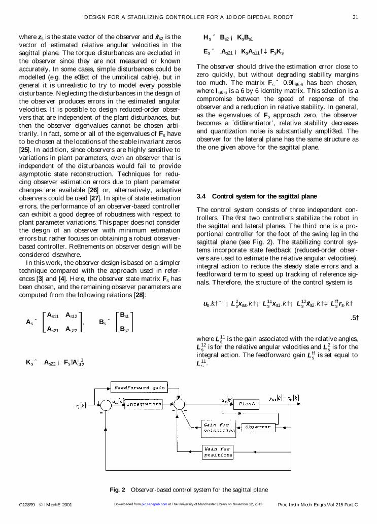
3.4 Control system for the sagittal plane

The control system consists of three independent con-

trollers. The ® rst two controllers stabilize the robot in

the sagittal and lateral planes. The third one is a pro-portional controller for the foot of the swing leg in the

sagittal plane (see Fig. 2). The stabilizing control sys-

tems incorporate state feedback (reduced-order obser-

vers are used to estimate the relative angular velocities),

integral action to reduce the steady state errors and afeedforward term to speed up tracking of reference sig-

nals. Therefore, the structure of the control system is

us…k† ˆ ¡L2sxas…k† ¡ L11

s xs1…k† ¡ L12s x̂s2…k† ‡ Lff

s rs…k†

…5†

where L11s is the gain associated with the relative angles,

L12s is for the relative angular velocities and L2

s is for the

integral action. The feedforward gain Lffs is set equal to

L11s .

Fig. 2 Observer-based control system for the sagittal plane

DESIGN FOR A STABILIZING CONTROLLER FOR A 10 DOF BIPEDAL ROBOT 31

C12899 ß IMechE 2001 Proc Instn Mech Engrs Vol 215 Part C at The University of Manchester Library on November 12, 2013pic.sagepub.comDownloaded from

The state-space representation of the integral action is

xas…k ‡ 1† ˆ ©asxas…k† ‡ ¡asuas…k†

uas…k† ˆ rs…k† ¡ xs1…k†

…6†

where xas is the state vector for the integrators, rs is the

vector of reference signals, which is set to zero in the

linear quadratic regulator design, ©as and ¡as are 6 £ 6identity matrices and xas, rs and xs1 are 6 £ 1 vectors.

The design of the optimal state feedback matrix starts

with the speci® cation of a quadratic performance index

J and the constraint equation. The objective is to

minimize J around the nominal operating point. The

performance index is in the form

Js ˆ1

kˆ0

xds…k†TQdsxds…k† ‡ us…k†TRdsus…k† …7†

where Qds and Rds are chosen as diagonal matrices with

positive entries. The constraint equation (ignoring tor-

que disturbances) is

xds…k ‡ 1† ˆ ©dsxds…k† ‡ ¡dsus…k† …8†

where

xds ˆxs

xas

©ds ˆAs 012£12

¡¡asCs ©as

¡ds ˆBs

06£6

The selection of Qds and Rds was investigated in Matlab

simulations and during experiments. The aims were to

achieve fast response with little or no overshoot and tomaintain the control signal within the power supply

limitations. The chosen values for Qds and Rds are

Qds ˆ Qsp Qsv Qsu

Qsp ˆ diag105 7 £ 104 5 £ 104

4 £ 105 3 £ 104 3 £ 104

Qsv ˆ 06£6

Qsu ˆ 10¡3I6£6

Rds ˆ I6£6

…9†

where Qsp is the matrix penalizing angular positions,

Qsv is for the velocities and Qsu is for the integralactions. In selecting Qsp, it was desirable for them to

be as low as possible to prevent demands for large

control actions. Low Qsp values increase relative sta-

bility and reduce sensitivity to noise. However, to

track reference signals with small errors and quickly

attenuate torque disturbances, relatively high values ofQsp are needed. Therefore, a compromise was made

between relative stability margins and the good

tracking of reference signals.

In order to minimize the control eŒorts, the matrix

penalizing velocities, Qsv, is set to zero. In the sagittalplane, gains for integral actions were kept to a mini-

mum. High integral gains tend to cause oscillations in

the system, mainly owing to the presence of backlash.

At present, tuning of the individual entries in Rds has

not been considered. One alternative would be to chooseRds taking into account the power of each actuator.

Once Qds and Rds are chosen, the optimal value J ¤s of

(7) is given in terms of the initial condition xs…0† and the

solution of the corresponding discrete-time algebraic

Riccati equation, P rics , i.e. J ¤

s ˆ xTs …0†P ric

s xs…0†.

3.5 Control system for the lateral plane

The control system has the same structure as the one for

the sagittal plane. The only diŒerence is that in the lat-

eral plane there are three links instead of six. The

matrices Qdl and Rdl for the performance index are

Qdl ˆ …Qlp†3£3 …Qlv†3£3 …Qlu†3£3

Qdl ˆ diag 104 104 104 0 0 0 1 1 19£9

Rdl ˆ I3£3

Owing to high static friction of the worm gearboxes used

for the lateral hip joints, the integral penalty matrix Qlu

is given higher values than those in the sagittal plane.

Bear in mind that excessive integral gain can causeoscillations.

4 RELATIVE STABILITY AND PERFORMANCE

This section investigates the robustness of the control

system through the analysis of Nyquist and singular-value plots. The state-space representation of the overall

32 D AKDAS AND G A MEDRANO-CERDA

Proc Instn Mech Engrs Vol 215 Part C C12899 ß IMechE 2001 at The University of Manchester Library on November 12, 2013pic.sagepub.comDownloaded from

controller can be written as follows (subscript s is used

for the sagittal plane and l for the lateral plane):

~as ˆFs ¡ HsL12

s ¡HsL2s

0 ©as

~bs ˆEs ¡ Hs L11

s ‡ L12s Ks

¡¡as

~cs ˆ ¡ L12s L2

s ; ~ds ˆ ¡ L11s ‡ L12

s Ks

~gs ˆHsL11

s

¡as

…10†De® ning

Gcs z… † ˆ ~cs zI ¡ ~as… †¡1 ~bs ‡ ~ds

Ns z… † ˆ ~cs zI ¡ ~as… †¡1 ~gs ‡ L11s

Gs…z† ˆ Cs…zI ¡ As†¡1Bs

Gdists …z† ˆ Cs…zI ¡ As†¡1Bdist

s

…11†Then, equations (2) and (5) can be written as

xs1 z… † ˆ Gs…z†u z… † ‡ Gdists ½½½½½s z… †

us z… † ˆ Gcs…z†‰xs1 z… † ‡ ns…z†Š ‡ Ns…z†rs z… †

…12†where, ns represents the quantization measurement

noise. The tilde in equations (10) and (11) is used toavoid using the same symbols to represent diŒerent

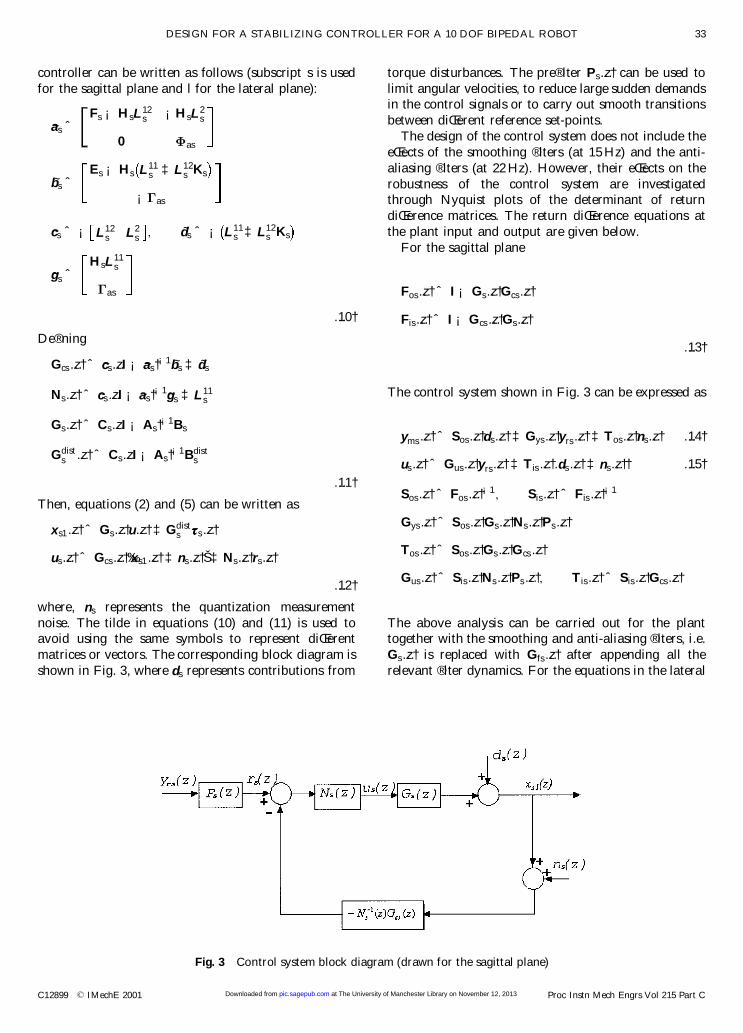
matrices or vectors. The corresponding block diagram is

shown in Fig. 3, where ds represents contributions from

torque disturbances. The pre® lter Ps z… † can be used to

limit angular velocities, to reduce large sudden demandsin the control signals or to carry out smooth transitions

between diŒerent reference set-points.

The design of the control system does not include the

eŒects of the smoothing ® lters (at 15 Hz) and the anti-

aliasing ® lters (at 22 Hz). However, their eŒects on the

robustness of the control system are investigatedthrough Nyquist plots of the determinant of return

diŒerence matrices. The return diŒerence equations at

the plant input and output are given below.

For the sagittal plane

Fos z… † ˆ I ¡ Gs z… †Gcs z… †

Fis z… † ˆ I ¡ Gcs z… †Gs z… †

…13†

The control system shown in Fig. 3 can be expressed as

yms z… † ˆ Sos z… †ds z… † ‡ Gys z… †yrs z… † ‡ Tos z… †ns z… † …14†

us z… † ˆ Gus z… †yrs z… † ‡ Tis z… † ds z… † ‡ ns z… †… † …15†

Sos z… † ˆ Fos z… †¡1; Sis z… † ˆ Fis z… †¡1

Gys z… † ˆ Sos z… †Gs z… †Ns z… †Ps z… †

Tos z… † ˆ Sos z… †Gs z… †Gcs z… †

Gus z… † ˆ Sis z… †Ns z… †Ps z… †; Tis z… † ˆ Sis z… †Gcs z… †

The above analysis can be carried out for the planttogether with the smoothing and anti-aliasing ® lters, i.e.

Gs z… † is replaced with Gfs z… † after appending all the

relevant ® lter dynamics. For the equations in the lateral

Fig. 3 Control system block diagram (drawn for the sagittal plane)

DESIGN FOR A STABILIZING CONTROLLER FOR A 10 DOF BIPEDAL ROBOT 33

C12899 ß IMechE 2001 Proc Instn Mech Engrs Vol 215 Part C at The University of Manchester Library on November 12, 2013pic.sagepub.comDownloaded from

plane, the subscript s is replaced by l. General infor-

mation about singular-value analysis can be found inreferences [29] and [30].

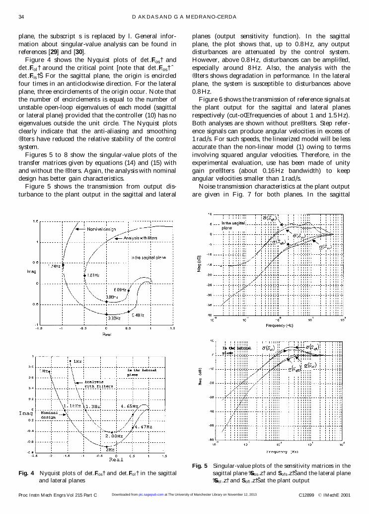
Figure 4 shows the Nyquist plots of det…Fos† and

det…Fol† around the critical point [note that det…Fos† ˆdet…Fis†Š. For the sagittal plane, the origin is encircled

four times in an anticlockwise direction. For the lateral

plane, three encirclements of the origin occur. Note thatthe number of encirclements is equal to the number of

unstable open-loop eigenvalues of each model (sagittal

or lateral plane) provided that the controller (10) has no

eigenvalues outside the unit circle. The Nyquist plots

clearly indicate that the anti-aliasing and smoothing® lters have reduced the relative stability of the control

system.

Figures 5 to 8 show the singular-value plots of the

transfer matrices given by equations (14) and (15) with

and without the ® lters. Again, the analysis with nominaldesign has better gain characteristics.

Figure 5 shows the transmission from output dis-

turbance to the plant output in the sagittal and lateral

planes (output sensitivity function). In the sagittal

plane, the plot shows that, up to 0.8 Hz, any outputdisturbances are attenuated by the control system.

However, above 0.8 Hz, disturbances can be ampli® ed,

especially around 8 Hz. Also, the analysis with the

® lters shows degradation in performance. In the lateral

plane, the system is susceptible to disturbances above

0.8 Hz.Figure 6 shows the transmission of reference signals at

the plant output for the sagittal and lateral planes

respectively (cut-oŒfrequencies of about 1 and 1.5 Hz).

Both analyses are shown without pre® lters. Step refer-

ence signals can produce angular velocities in excess of1 rad/s. For such speeds, the linearized model will be less

accurate than the non-linear model (1) owing to terms

involving squared angular velocities. Therefore, in the

experimental evaluation, use has been made of unity

gain pre® lters (about 0.16 Hz bandwidth) to keepangular velocities smaller than 1 rad/s.

Noise transmission characteristics at the plant output

are given in Fig. 7 for both planes. In the sagittal

Fig. 4 Nyquist plots of det…Fos† and det…Fol† in the sagittal

and lateral planes

Fig. 5 Singular-value plots of the sensitivity matrices in the

sagittal plane ‰Sos…z† and Sofs…z†Š and the lateral plane

‰Sol…z† and Sofl…z†Š at the plant output

34 D AKDAS AND G A MEDRANO-CERDA

Proc Instn Mech Engrs Vol 215 Part C C12899 ß IMechE 2001 at The University of Manchester Library on November 12, 2013pic.sagepub.comDownloaded from

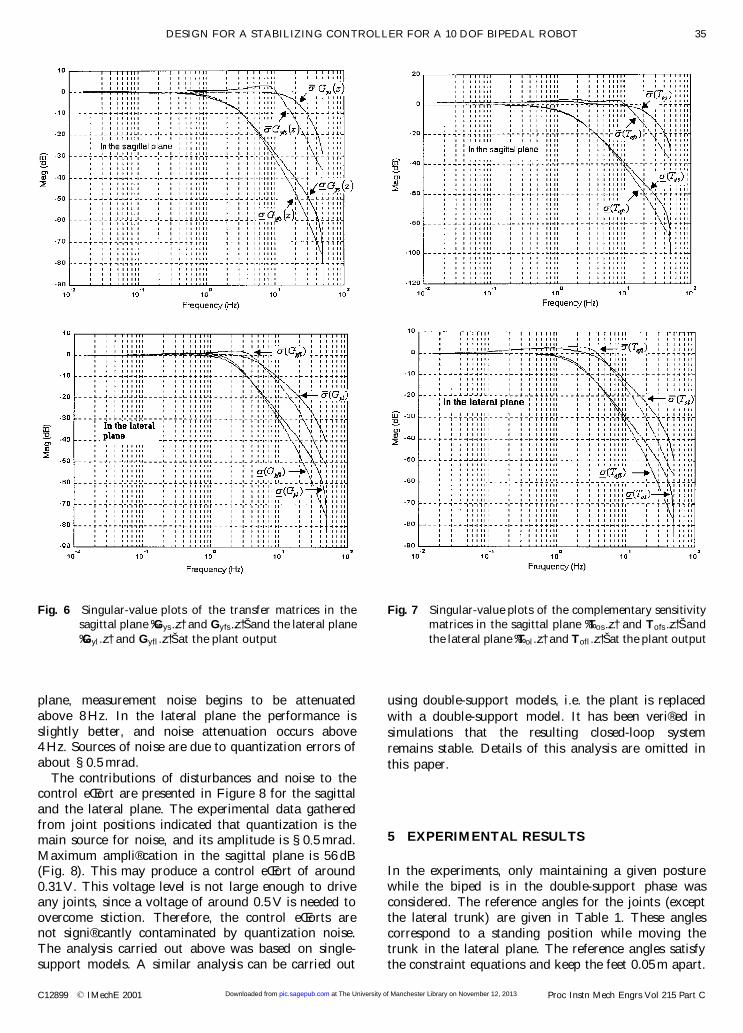
plane, measurement noise begins to be attenuatedabove 8 Hz. In the lateral plane the performance isslightly better, and noise attenuation occurs above4 Hz. Sources of noise are due to quantization errors ofabout §0:5 mrad.

The contributions of disturbances and noise to thecontrol eŒort are presented in Figure 8 for the sagittaland the lateral plane. The experimental data gatheredfrom joint positions indicated that quantization is themain source for noise, and its amplitude is §0:5 mrad.Maximum ampli® cation in the sagittal plane is 56 dB(Fig. 8). This may produce a control eŒort of around0.31 V. This voltage level is not large enough to driveany joints, since a voltage of around 0.5 V is needed toovercome stiction. Therefore, the control eŒorts arenot signi® cantly contaminated by quantization noise.The analysis carried out above was based on single-support models. A similar analysis can be carried out

using double-support models, i.e. the plant is replaced

with a double-support model. It has been veri® ed in

simulations that the resulting closed-loop system

remains stable. Details of this analysis are omitted in

this paper.

5 EXPERIMENTAL RESULTS

In the experiments, only maintaining a given posturewhile the biped is in the double-support phase wasconsidered. The reference angles for the joints (exceptthe lateral trunk) are given in Table 1. These anglescorrespond to a standing position while moving thetrunk in the lateral plane. The reference angles satisfythe constraint equations and keep the feet 0.05 m apart.

Fig. 6 Singular-value plots of the transfer matrices in the

sagittal plane ‰Gys…z† and Gyfs…z†Š and the lateral plane

‰Gyl…z† and Gyfl…z†Š at the plant output

Fig. 7 Singular-value plots of the complementary sensitivity

matrices in the sagittal plane ‰Tos…z† and Tofs…z†Š and

the lateral plane ‰Tol…z† and Tofl…z†Š at the plant output

DESIGN FOR A STABILIZING CONTROLLER FOR A 10 DOF BIPEDAL ROBOT 35

C12899 ß IMechE 2001 Proc Instn Mech Engrs Vol 215 Part C at The University of Manchester Library on November 12, 2013pic.sagepub.comDownloaded from

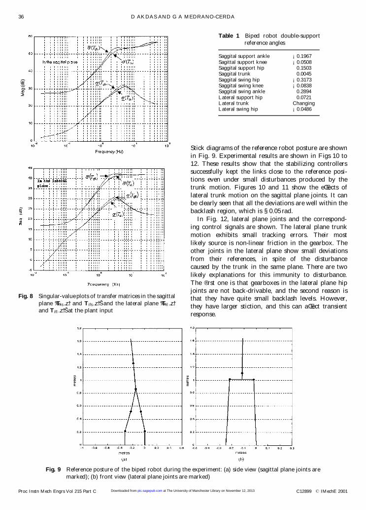
Stick diagrams of the reference robot posture are shown

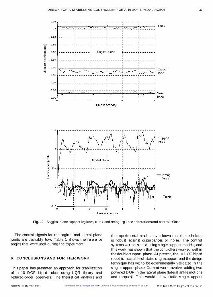
in Fig. 9. Experimental results are shown in Figs 10 to

12. These results show that the stabilizing controllers

successfully kept the links close to the reference posi-

tions even under small disturbances produced by the

trunk motion. Figures 10 and 11 show the eŒects of

lateral trunk motion on the sagittal plane joints. It can

be clearly seen that all the deviations are well within the

backlash region, which is §0:05 rad.

In Fig. 12, lateral plane joints and the correspond-

ing control signals are shown. The lateral plane trunk

motion exhibits small tracking errors. Their most

likely source is non-linear friction in the gearbox. The

other joints in the lateral plane show small deviations

from their references, in spite of the disturbance

caused by the trunk in the same plane. There are two

likely explanations for this immunity to disturbance.

The ® rst one is that gearboxes in the lateral plane hip

joints are not back-drivable, and the second reason isthat they have quite small backlash levels. However,

they have larger stiction, and this can aŒect transient

response.

Fig. 8 Singular-value plots of transfer matrices in the sagittal

plane ‰Tis…z† and Tifs…z†Š and the lateral plane ‰Til…z†and Tifl…z†Š at the plant input

Table 1 Biped robot double-support

reference angles

Saggital support ankle ¡0:1967Sagittal support knee ¡0:0508Saggital support hip 0.1503Saggital trunk 0.0045Saggital swing hip ¡0:3173Saggital swing knee ¡0:0838Saggital swing ankle 0.2894Lateral support hip 0.0721Lateral trunk ChangingLateral swing hip ¡0:0486

Fig. 9 Reference posture of the biped robot during the experiment: (a) side view (sagittal plane joints are

marked); (b) front view (lateral plane joints are marked)

36 D AKDAS AND G A MEDRANO-CERDA

Proc Instn Mech Engrs Vol 215 Part C C12899 ß IMechE 2001 at The University of Manchester Library on November 12, 2013pic.sagepub.comDownloaded from

The control signals for the sagittal and lateral plane

joints are desirably low. Table 1 shows the reference

angles that were used during the experiment.

6 CONCLUSIONS AND FURTHER WORK

This paper has presented an approach for stabilization

of a 10 DOF biped robot using LQR theory andreduced-order observers. The theoretical analysis and

the experimental results have shown that the technique

is robust against disturbances or noise. The control

systems were designed using single-support models, andthis work has shown that the controllers worked well in

the double-support phase. At present, the 10 DOF biped

robot is incapable of static single support and the design

technique has yet to be experimentally validated in the

single-support phase. Current work involves adding two

powered DOF in the lateral plane (lateral ankle motionsand torques). This would allow static single-support

Fig. 10 Saggital plane support-leg knee, trunk and swing-leg knee orientations and control eŒorts

DESIGN FOR A STABILIZING CONTROLLER FOR A 10 DOF BIPEDAL ROBOT 37

C12899 ß IMechE 2001 Proc Instn Mech Engrs Vol 215 Part C at The University of Manchester Library on November 12, 2013pic.sagepub.comDownloaded from

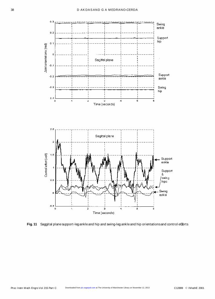
Fig. 11 Saggital plane support-leg ankle and hip and swing-leg ankle and hip orientations and control eŒorts

38 D AKDAS AND G A MEDRANO-CERDA

Proc Instn Mech Engrs Vol 215 Part C C12899 ß IMechE 2001 at The University of Manchester Library on November 12, 2013pic.sagepub.comDownloaded from

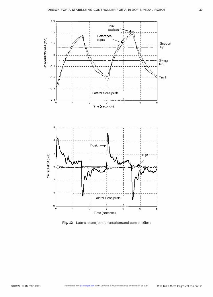
Fig. 12 Lateral plane joint orientations and control eŒorts

DESIGN FOR A STABILIZING CONTROLLER FOR A 10 DOF BIPEDAL ROBOT 39

C12899 ß IMechE 2001 Proc Instn Mech Engrs Vol 215 Part C at The University of Manchester Library on November 12, 2013pic.sagepub.comDownloaded from

balance and give the robot the capability to climb stairs

and walk at low speeds, as well as making dynamicwalking smoother. In addition, the control system was

capable of maintaining joint positions close to given

reference values under small torque disturbances. For

large torque disturbances the biped did not remain

standing. This failure was due to the lack of information

about ground reaction forces. It is clear that groundreaction force measurements are essential to maintain

equilibrium in realistic situations.

REFERENCES

1 Hirai, K., Hirose, M., Haikawa, Y. and Takenaka, T. The

development of Honda humanoid robot. In IEEE Inter-

national Conference on Robotics and Automation, Leuven,

Belgium, May 1998, Vol. 2, pp. 1321± 1326.

2 Mita, T., Yamaguchi, T., Kashiwase, T. and Kawase, T.

Realization of a high speed biped using modern control

theory. Int. J. Control, 1984, 40(1), 107± 119.

3 Eldukhri, E. E. Design and control of a biped walking

robot. PhD thesis, Department of Electronic and Electrical

Engineering, University of Salford, UK.

4 Medrano-Cerda, G. A. and Eldukhri, E. E. Biped robot

locomotion in the sagittal plane. Trans. Inst. Measmt and

Control, 1997, 19(1), 38± 49.

5 Hemami, H. and Wyman, B. F. Modeling and control of

constrained dynamic systems with application to biped

locomotion in the frontal plane. IEEE Trans. Autom.

Control, 1979, AC-24(4), 527± 535.

6 Golliday Jr, C. L. and Hemami, H. Postural stability of the

two-degree of freedom biped by general linear feedback.

IEEE Trans. Autom. Control, 1976, AC-21(1), 74± 79.

7 Raibert, M. H. Legged Robots that Balance, 1986 (MIT

Press, Cambridge, Massachusetts).

8 Golliday Jr, C. L. and Hemami, H. An approach to

analyzing biped locomotion dynamics and designing robot

locomotion controls. IEEE Trans. Autom. Control, 1977,

AC-22(6), 963± 972.

9 Raibert, M. H., Tzafestas, S. and Tzafestas, C. Compara-

tive simulation study of three control techniques applied to

a biped robot. In IEEE International Conference on

Systems, Man and Cybernetics, Le Touquet, France,

October 1993, Vol. 1, pp. 494± 502.

10 Miura, H. and Shimoyama, I. Dynamic walk of a robot.

Int. J. Robotics Res., 1984, 3(2), 60± 74.

11 Channon, P. H., Hopkins, S. H. and Pham, D. T.

Modelling and control of a bipedal robot. J. Syst.

Engng, 1992, 2, 46± 59.

12 Inaba, M., Kanehiro, F., Kagami, S. and Inoue, H. Two-

armed bipedal robot that can walk, roll over and stand up.

In IROS’95 International Conference on Intelligent Robots

and System, Pittsburgh, Pennsylvania, 1995, Vol. 3, pp.

297± 302.

13 Fukuda, T., Komata, Y. and Arakawa, T. Stabilisation

control of biped locomotion robot based learning with Gas

having self-adaptive mutation and recurrent neural net-

works. In IEEE International Conference on Robotics and

Automation, Albuquerque, New Mexico, April 1997, Vol.

1, pp. 217± 222.

14 Kun, A. and Miller, W. T. Adaptive dynamic balance of a

biped robot using neural networks. In IEEE International

Conference on Robotics and Automation, Minneapolis,

Minnesota, April 1996, pp. 240± 245.

15 Salatian, A. W. and Zheng, Y. F. Gait synthesis for a biped

robot climbing sloping surfaces using neural networks. In

IEEE International Conference on Robotics and Auto-

mation, Nice, France, May 1992, pp. 2601± 2606.

16 Vukobratovic, M., Borovac, B., Surla, D. and Stokic, D.

Biped Locomotion: Dynamics, Stability, Control and

Application, 1990 (Springer-Verlag, Berlin).

17 Takanishi, A., Ishida, M., Yamazaki, Y. and Kato, I. The

realization of dynamic walking by the biped walking robot

WL-10RD. In International Conference on Advanced

Robotics, Tokyo, 1985, pp. 459± 466.

18 Takanishi, A., Tochizawa, M., Takeya, T., Kanaki, H. and

Kato, I. Realization of dynamic biped walking stabilized

with trunk motion under known external force. In 4th

International Conference on Advanced Robotics, Colum-

bus, Ohio, 1990; in ScientiWc Fundamentals of Robotics 7

(Ed. K. J. Waldron), 1990, pp. 299± 310 (Springer-Verlag,

Berlin).

19 Li, Q., Takanishi, A. and Kato, I. Learning control for a

biped walking robot with a trunk. In IEEE International

Conference on Intelligent Robots and Systems, Yokohama,

Japan, July 1993, pp. 1171± 1777.

20 Yamaguchi, J., Takanishi, A. and Kato, I. Development of

a biped walking robot compensating for three-axis

moment by trunk motion. In IEEE International Con-

ference on Robotics and Automation, Yokohama, Japan,

July 1993, pp. 561-566.

21 Yamaguchi, J., Kinoshita, N., Takanishi A. and Kato, I.

Development of a dynamic biped walking system for

humanoid: development of a biped walking robot adapting

to the humans’ living ¯ oor. In IEEE International

Conference on Robotics and Automation, Minneapolis,

Minnesota, April 1996, pp. 232± 239.

22 Yamaguchi, J., Soga, E., Inoue, S. and Takanishi, A.

Developmentof a bipedal humanoid robot: control method

of whole body co-operative dynamic biped walking.

In IEEE International Conference on Robotics and

Automation, Detroit, Michigan, May 1999, pp. 368-374.

23 Amirouche, F. M. L. Computational Methods in Multibody

Dynamics, 1992 (Prentice-Hall, Englewood CliŒs, New

Jersey).

24 Shih, C. L. and Gruver, W. A. Control of a biped robot in

the double-support phase. IEEE Trans. Syst. Man and

Cybernetics, 1992, SMC-22(4), 729± 735.

25 Kudva, P., Viswanadham, N. and Ramakrishna, A.

Observers for linear systems with unknown inputs. IEEE

Trans. Autom. Control, 1980, AC-25(1), 113± 115.

26 Wang, S. D., Kuo, T. S. and Hsu, C. F. Optimal observer

design for linear dynamical systems with uncertain

parameters. Int. J. Control, 1987, 45(2), 701± 711.

27 O’Reilly, J. Observers for Linear Systems, 1983 (Academic

Press, London).

28 Vaccaro, R. J. Digital Control, a State-Space Approach,

1995 (McGraw-Hill, Singapore).

29 Maciejowski, J. M. Multivariable Feedback Design, 1989

(Addison-Wesley, Cornwall).

30 Skogestad, S. and Postlethwaite, I. Multivariable Feedback

Control (John Wiley, Chichester).

40 D AKDAS AND G A MEDRANO-CERDA

Proc Instn Mech Engrs Vol 215 Part C C12899 ß IMechE 2001 at The University of Manchester Library on November 12, 2013pic.sagepub.comDownloaded from

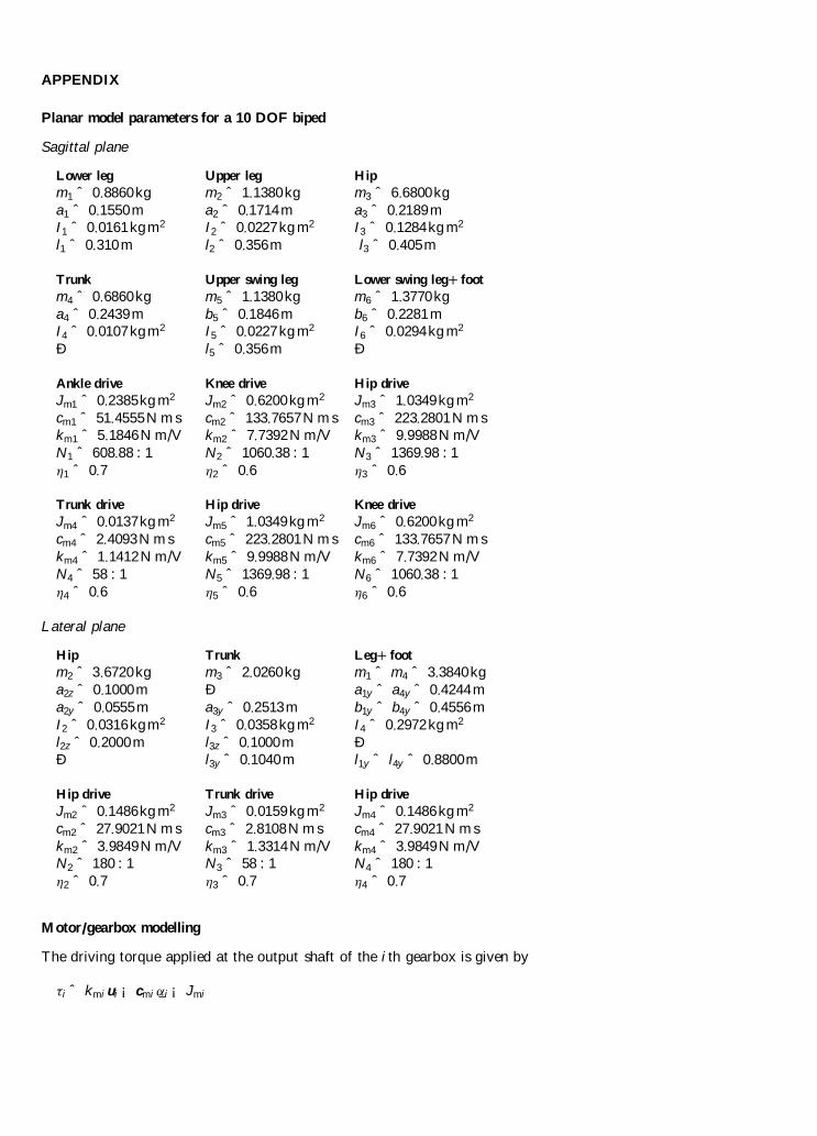
APPENDIX

Planar model parameters for a 10 DOF biped

Sagittal plane

Lower leg Upper leg Hip

m1 ˆ 0:8860 kg m2 ˆ 1:1380 kg m3 ˆ 6:6800 kg

a1 ˆ 0:1550 m a2 ˆ 0:1714 m a3 ˆ 0:2189 mI1 ˆ 0:0161 kg m2 I2 ˆ 0:0227 kg m2 I3 ˆ 0:1284 kg m2

l1 ˆ 0:310 m l2 ˆ 0:356m l3 ˆ 0:405m

Trunk Upper swing leg Lower swing leg 1 foot

m4 ˆ 0:6860 kg m5 ˆ 1:1380 kg m6 ˆ 1:3770 kg

a4 ˆ 0:2439 m b5 ˆ 0:1846 m b6 ˆ 0:2281 mI4 ˆ 0:0107 kg m2 I5 ˆ 0:0227 kg m2 I6 ˆ 0:0294 kg m2

Ð l5 ˆ 0:356m Ð

Ankle drive Knee drive Hip drive

Jm1 ˆ 0:2385kg m2 Jm2 ˆ 0:6200 kg m2 Jm3 ˆ 1:0349 kg m2

cm1 ˆ 51:4555 N m s cm2 ˆ 133:7657 N m s cm3 ˆ 223:2801 N m skm1 ˆ 5:1846 N m/V km2 ˆ 7:7392 N m/V km3 ˆ 9:9988 N m/VN1 ˆ 608:88 : 1 N2 ˆ 1060:38 : 1 N3 ˆ 1369:98 : 1

²1 ˆ 0:7 ²2 ˆ 0:6 ²3 ˆ 0:6

Trunk drive Hip drive Knee drive

Jm4 ˆ 0:0137kg m2 Jm5 ˆ 1:0349 kg m2 Jm6 ˆ 0:6200 kg m2

cm4 ˆ 2:4093 N m s cm5 ˆ 223:2801 N m s cm6 ˆ 133:7657 N m s

km4 ˆ 1:1412 N m/V km5 ˆ 9:9988 N m/V km6 ˆ 7:7392 N m/VN4 ˆ 58 : 1 N5 ˆ 1369:98 : 1 N6 ˆ 1060:38 : 1

²4 ˆ 0:6 ²5 ˆ 0:6 ²6 ˆ 0:6

Lateral plane

Hip Trunk Leg 1 foot

m2 ˆ 3:6720 kg m3 ˆ 2:0260 kg m1 ˆ m4 ˆ 3:3840 kg

a2z ˆ 0:1000 m Ð a1y ˆ a4y ˆ 0:4244 m

a2y ˆ 0:0555 m a3y ˆ 0:2513 m b1y ˆ b4y ˆ 0:4556 m

I2 ˆ 0:0316 kg m2 I3 ˆ 0:0358 kg m2 I4 ˆ 0:2972 kg m2

l2z ˆ 0:2000 m l3z ˆ 0:1000 m ÐÐ l3y ˆ 0:1040 m l1y ˆ l4y ˆ 0:8800m

Hip drive Trunk drive Hip drive

Jm2 ˆ 0:1486kg m2 Jm3 ˆ 0:0159 kg m2 Jm4 ˆ 0:1486 kg m2

cm2 ˆ 27:9021 N m s cm3 ˆ 2:8108 N m s cm4 ˆ 27:9021 N m s

km2 ˆ 3:9849 N m/V km3 ˆ 1:3314 N m/V km4 ˆ 3:9849 N m/VN2 ˆ 180 : 1 N3 ˆ 58 : 1 N4 ˆ 180 : 1

²2 ˆ 0:7 ²3 ˆ 0:7 ²4 ˆ 0:7

Motor/gearbox modelling

The driving torque applied at the output shaft of the i th gearbox is given by

½i ˆ kmi ui ¡ cmi _¬i ¡ Jmi �¬i

where _¬i and �¬i are the relative angular velocity and acceleration of the i th joint, ui is the applied motor voltage, kmi is

the motor gain, cmi is the motor damping re¯ ected at the output shaft and Jmi is the motor inertia re¯ ected at theoutput shaft. In the present calculations the motor inductance and the gearbox inertia are neglected.

DESIGN FOR A STABILIZING CONTROLLER FOR A 10 DOF BIPEDAL ROBOT 41

C12899 ß IMechE 2001 Proc Instn Mech Engrs Vol 215 Part C at The University of Manchester Library on November 12, 2013pic.sagepub.comDownloaded from

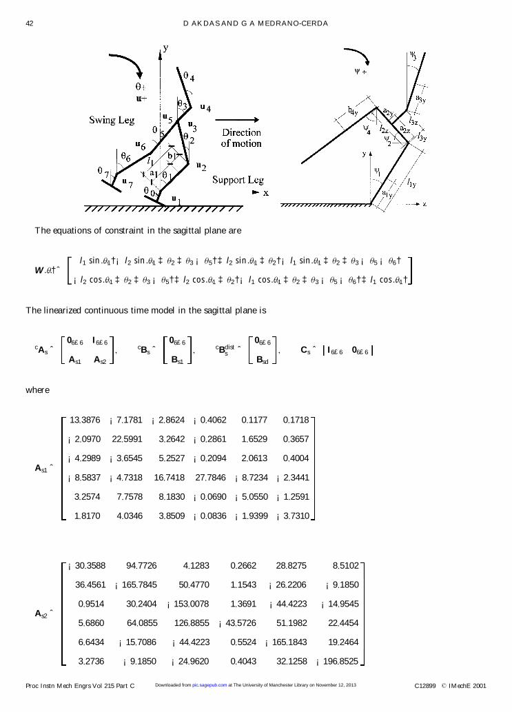
The equations of constraint in the sagittal plane are

W…³† ˆl1 sin…³1† ¡ l2 sin…³1 ‡ ³2 ‡ ³3 ¡ ³5† ‡ l2 sin…³1 ‡ ³2† ¡ l1 sin…³1 ‡ ³2 ‡ ³3 ¡ ³5 ¡ ³6†

¡l2 cos…³1 ‡ ³2 ‡ ³3 ¡ ³5† ‡ l2 cos…³1 ‡ ³2† ¡ l1 cos…³1 ‡ ³2 ‡ ³3 ¡ ³5 ¡ ³6† ‡ l1 cos…³1†

The linearized continuous time model in the sagittal plane is

cAs ˆ06£6 I6£6

As1 As2

; cBs ˆ06£6

Bs1

; cBdists ˆ

06£6

Bsd

; Cs ˆ I6£6 06£6

where

As1 ˆ

13:3876 ¡7:1781 ¡2:8624 ¡0:4062 0:1177 0:1718

¡2:0970 22:5991 3:2642 ¡0:2861 1:6529 0:3657

¡4:2989 ¡3:6545 5:2527 ¡0:2094 2:0613 0:4004

¡8:5837 ¡4:7318 16:7418 27:7846 ¡8:7234 ¡2:3441

3:2574 7:7578 8:1830 ¡0:0690 ¡5:0550 ¡1:2591

1:8170 4:0346 3:8509 ¡0:0836 ¡1:9399 ¡3:7310

As2 ˆ

¡30:3588 94:7726 4:1283 0:2662 28:8275 8:5102

36:4561 ¡165:7845 50:4770 1:1543 ¡26:2206 ¡9:1850

0:9514 30:2404 ¡153:0078 1:3691 ¡44:4223 ¡14:9545

5:6860 64:0855 126:8855 ¡43:5726 51:1982 22:4454

6:6434 ¡15:7086 ¡44:4223 0:5524 ¡165:1843 19:2464

3:2736 ¡9:1850 ¡24:9620 0:4043 32:1258 ¡196:8525

42 D AKDAS AND G A MEDRANO-CERDA

Proc Instn Mech Engrs Vol 215 Part C C12899 ß IMechE 2001 at The University of Manchester Library on November 12, 2013pic.sagepub.comDownloaded from

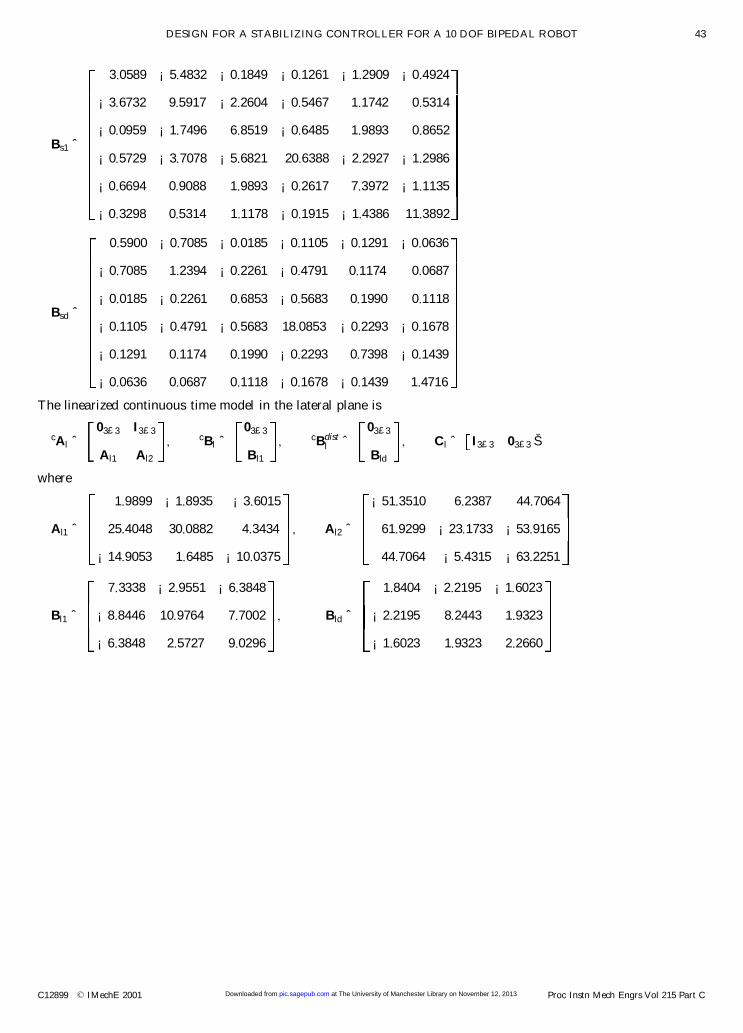
Bs1 ˆ

3:0589 ¡5:4832 ¡0:1849 ¡0:1261 ¡1:2909 ¡0:4924

¡3:6732 9:5917 ¡2:2604 ¡0:5467 1:1742 0:5314

¡0:0959 ¡1:7496 6:8519 ¡0:6485 1:9893 0:8652

¡0:5729 ¡3:7078 ¡5:6821 20:6388 ¡2:2927 ¡1:2986

¡0:6694 0:9088 1:9893 ¡0:2617 7:3972 ¡1:1135

¡0:3298 0:5314 1:1178 ¡0:1915 ¡1:4386 11:3892

Bsd ˆ

0:5900 ¡0:7085 ¡0:0185 ¡0:1105 ¡0:1291 ¡0:0636

¡0:7085 1:2394 ¡0:2261 ¡0:4791 0:1174 0:0687

¡0:0185 ¡0:2261 0:6853 ¡0:5683 0:1990 0:1118

¡0:1105 ¡0:4791 ¡0:5683 18:0853 ¡0:2293 ¡0:1678

¡0:1291 0:1174 0:1990 ¡0:2293 0:7398 ¡0:1439

¡0:0636 0:0687 0:1118 ¡0:1678 ¡0:1439 1:4716

The linearized continuous time model in the lateral plane is

cAl ˆ03£3 I3£3

Al1 Al2

; cBl ˆ03£3

Bl1

; cBdistl ˆ

03£3

Bld

; Cl ˆ I3£3 03£3 Š

where

Al1 ˆ

1:9899 ¡1:8935 ¡3:6015

25:4048 30:0882 4:3434

¡14:9053 1:6485 ¡10:0375

; Al2 ˆ

¡51:3510 6:2387 44:7064

61:9299 ¡23:1733 ¡53:9165

44:7064 ¡5:4315 ¡63:2251

Bl1 ˆ

7:3338 ¡2:9551 ¡6:3848

¡8:8446 10:9764 7:7002

¡6:3848 2:5727 9:0296

; Bld ˆ

1:8404 ¡2:2195 ¡1:6023

¡2:2195 8:2443 1:9323

¡1:6023 1:9323 2:2660

DESIGN FOR A STABILIZING CONTROLLER FOR A 10 DOF BIPEDAL ROBOT 43

C12899 ß IMechE 2001 Proc Instn Mech Engrs Vol 215 Part C at The University of Manchester Library on November 12, 2013pic.sagepub.comDownloaded from