Design of experiment and Response surface methodology

Design Of Experiment (DOE) &

Response Surface Methodology (RSM)

Present by:

Wan Nor Nadyaini Wan Omar,

B.Eng (Chem),M.Eng (Chem)Faculty of Chemical Engineering

([email protected])

Date: 12 Aug 2015

Place: N29,,Faculty of Chemical Engineering

12/8/2015 1academia@DahliaOmar

IF??


Research Cycle processAsk Question:

Objective of study

Data Collection

Experimental Design

Graphical analysis

Analyze the result to answer the

question


DATA COLLECTIONTo clarify the objective of experiment

• What data to be collected?• How to measure it?• How the data relates to process performances

and experimental objective?

The experimenter must determine

• Thus, the data could lead to correct conclusion

The experimenter must ensure the data collected is represented the processThe experimenter must ensure the data collected is represented the process

The experimental design must related to experimental objectivesThe experimental design must related to experimental objectives


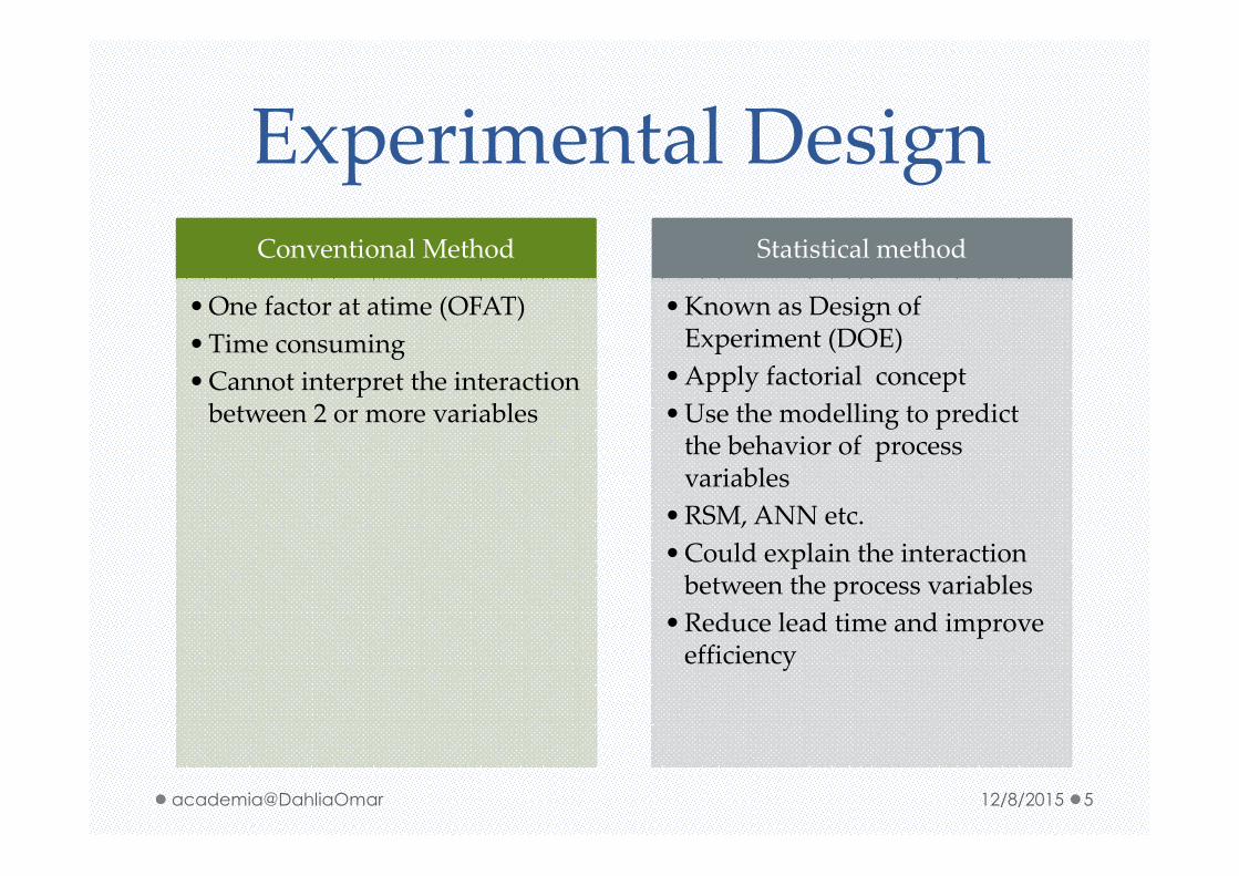
Experimental DesignConventional Method

• One factor at atime (OFAT)• Time consuming• Cannot interpret the interaction

between 2 or more variables

Statistical method

• Known as Design of Experiment (DOE)

• Apply factorial concept • Use the modelling to predict

the behavior of process variables

• RSM, ANN etc.• Could explain the interaction

between the process variables• Reduce lead time and improve

efficiency


Response Surface Methodology (RSM) is a statistic techniques employed a regression analysis to performed for the collective data.

• is a tools to help we designs our experiment and analyses our data.

• RSM is one of the technique that have been programmed in that software.

What is STATISTICA, Design Expert, MiniTaband etc?

What is RSM?

What is DOE?A collection of predetermined process variables setting


What DOE & RSM can do?

PREDICTION

• Could predict the relationship/interaction between the values of some measureable response variable(s) and those of a set of experimental factors presumed to affect the response(s)

• Predict the response value at various process condition

OPTIMIZATION

• Could find the values of the factors that produces the best value or values of the response(s).


Flow of RSM study

Experiment

DOE spreadsheet

Mathematical model

Validity of Data

Variable selection

Find relationship

Optimization

Design of

experiment

(DOE)

Analysis of

Data


Step in RSM studyBefore: Select the

variable-Design the experiment

During: The actual experiment will be

carried out

After: Analyze the data.


Before Experiment

1. Selecting the process variables

2. Selecting the level and range for each process variable

3. Selecting the design of experiment (DOE)12/8/2015 10academia@DahliaOmar

Preparing for RSM study•What response variables are to be measured, how they will be

measured, and in what sequence?RESPONSE

•Which factor are most important and therefore will be included in the experiment, and which are least important and can these factor be omitted? With the important factors, can the desired effects be detected?

PROCESS VARIABLE

•What extraneous or disturbing factors must be controlled or at least have their effects minimized?DISTURBANCE

•What is the experimental unit, that is to say, what is the piece of experimental material from which a response value is measured? How are the experimental units to be replicated, if at all?

EXPERIMENTAL UNIT

•The choice of the factors and level determined the type, size and experimental region. The no. of level at each factor as well as the no. of replicated experiment units represent the total no. of experiment.

DESICION


Design of experiment (DOE) Process

Objective

• Screening • Prediction• Optimization

Factor

• No of Independent Var.

• Block• Level • Range

Type of design

• Full factorial• Fractional factorial• Placket Burman• CCD• Box-behnken• Taguchi• Etc.


Objective

• To identify significant main effect of factors from a list of many potential ones

• Not identified the interaction effect• Type of design: 2-level with resolution III or IV, fractional

factorial, Plackett-Burman

• To identify significant main effect of factors from a list of many potential ones

• Not identified the interaction effect• Type of design: 2-level with resolution III or IV, fractional

factorial, Plackett-Burman

Screening

• To identify the best process performance, interaction effect, and significant of factors

• Type of design: CCD or BBD

• To identify the best process performance, interaction effect, and significant of factors

• Type of design: CCD or BBD

Optimization


1) Selecting the Parameter

• Process conditions influence the value of response variable• Can be qualitative or quantitative• Qualitative-blocking variables• Quantitative –normally considered in RSM

• Process conditions influence the value of response variable• Can be qualitative or quantitative• Qualitative-blocking variables• Quantitative –normally considered in RSM

Factors:

• The measureable quantity whose value is assumed to be affected by changing the levels of the factors and most interested in optimizing.

• The measureable quantity whose value is assumed to be affected by changing the levels of the factors and most interested in optimizing.

Responses:


2) Selecting the Level

Two level (2k) - (-1,+1)-first order,

• Two-level factorial design is each factor is evaluated at a “low” setting and at “high” setting.

Three level (3k) – (-1,0,+1) second or higher order

• Three-level factorial design is each factor is evaluated at a “low”, “center” and at “high” setting.

Five-level (5k)-(-α, -1,0,+1, -α) second or higher order

• Five-level factorial design is each factor is evaluated at a “Star low”, “low”, “center” , “high” and “star high” setting.


Experimental region o The region of conceivable factor level values that represents the factor combinations of potential interest.

o Need to determined before the experiment by finding the range of variables.

o If at the end of analysis, the factor value or optimum is out of the range, the experiment need to repeat with the new range.

Factors SymbolRange and Levels

-1 0 +1Molar ratio methanol: oil X1 20:1 30:1 40:1

Catalyst loading, wt% X2 2 3 4Reaction Time, min X3 120 180 240

Reaction Temperature X4 90 120 15012/8/2015 16academia@DahliaOmar

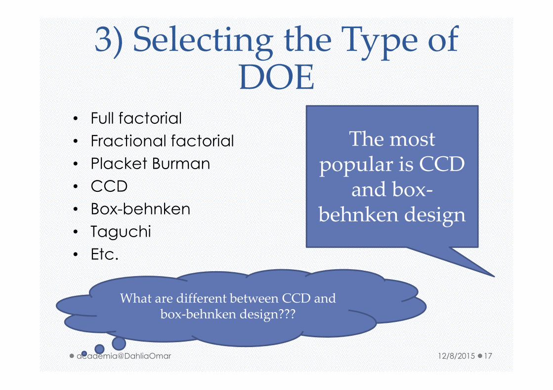
3) Selecting the Type of DOE

• Full factorial

• Fractional factorial

• Placket Burman

• CCD

• Box-behnken

• Taguchi

• Etc.

What are different between CCD and box-behnken design???

The most popular is CCD

and box-behnken design


Factorial design

Easy to be used by simply following relatively simple design

Able to meet the majority of the experimental needs and its data analysis can be performed by graphical methods

Require relatively few runs at a reasonable size

If large number of factors is selected, the fractional factorial design can be employed to keep thea experimental run at a reasonable size


Full factorial & fractional factorial

• Two level Full factorial (-1,+1)= 2k

• Three level full factorial (-1,0,+1) =3k

• Fractional factorial (two level) = 2k-m, m<ko ½= 2k-1

o 1/4= 2k-2

o 1/8= 2k-4

• Fractional factorial (three level) = 3k-m, m<k

Rotatable

Orthogonal


Matrix Arrangement(2-level)

A B C D1 -1 -1 -1 -12 1 -1 -1 13 -1 1 -1 14 1 1 -1 -15 -1 -1 1 16 1 -1 1 -17 -1 1 1 -18 1 1 1 1

A B C D1 -1 -1 -1 -12 1 -1 -1 -13 -1 1 -1 -14 1 1 -1 -15 -1 -1 1 -16 1 -1 1 -17 -1 1 1 -18 1 1 1 -19 -1 -1 -1 110 1 -1 -1 111 -1 1 -1 112 1 1 -1 113 -1 -1 1 114 1 -1 1 115 -1 1 1 116 1 1 1 1

2-level fractional fractorial design (resolution IV)

2-level factorial design (full)


Matrix Arrangement(3-level)

3**(4-0) full factorial design, 1 block , 81 runs (Spreadsheet1)

A B C D1 -1 -1 -1 -12 -1 -1 -1 0

3 -1 -1 -1 14 -1 -1 0 -15 -1 -1 0 06 -1 -1 0 17 -1 -1 1 -18 -1 -1 1 067 1 0 0 -168 1 0 0 069 1 0 0 170 1 0 1 -171 1 0 1 072 1 0 1 173 1 1 -1 -174 1 1 -1 075 1 1 -1 176 1 1 0 -177 1 1 0 078 1 1 0 179 1 1 1 -180 1 1 1 081 1 1 1 1

3**(4-1) fractional factorial design, 1 block , 27 runs (Spreadsheet1)

A B C D

1 -1 -1 -1 -1

2 -1 -1 0 1

3 -1 -1 1 0

4 -1 0 -1 1

5 -1 0 0 0

6 -1 0 1 -1

7 -1 1 -1 0

8 -1 1 0 -1

9 -1 1 1 1

10 0 -1 -1 1

11 0 -1 0 0

12 0 -1 1 -1

18 0 1 1 0

19 1 -1 -1 0

20 1 -1 0 -1

21 1 -1 1 1

22 1 0 -1 -1

23 1 0 0 1

24 1 0 1 0

25 1 1 -1 1

26 1 1 0 0

27 1 1 1 -1

3**(4-1) fractional factorial design, 3 blocks, 27 runs (Spreadsheet1)

Block A B C D

1 1 1 0 -1 -1

2 1 0 1 0 1

3 1 -1 -1 0 1

4 1 0 1 -1 -1

5 1 1 0 0 1

6 1 -1 -1 1 0

13 2 0 -1 1 -1

14 2 0 -1 0 0

15 2 0 -1 -1 1

16 2 1 1 0 0

17 2 -1 0 -1 1

18 2 1 1 1 -1

19 3 0 0 1 1

20 3 0 0 0 -1

21 3 -1 1 -1 0

22 3 0 0 -1 0

23 3 1 -1 1 1

24 3 1 -1 0 -1

25 3 1 -1 -1 0

26 3 -1 1 1 1

27 3 -1 1 0 -1

3**(4-1) fractional factorial design, 9 blocks, 27 runs (Spreadsheet1)

Block A B C D

1 1 0 1 0 1

2 1 1 0 1 0

5 2 1 0 0 1

6 2 0 1 -1 -1

7 3 1 0 -1 -1

8 3 -1 -1 0 1

11 4 -1 0 -1 1

12 4 1 1 1 -1

13 5 -1 0 1 -1

14 5 1 1 0 0

15 5 0 -1 -1 1

16 6 1 1 -1 1

17 6 0 -1 1 -1

18 6 -1 0 0 0

19 7 -1 1 -1 0

20 7 0 0 0 -1

21 7 1 -1 1 1

22 8 0 0 -1 0

23 8 1 -1 0 -1

24 8 -1 1 1 1

25 9 0 0 1 1

26 9 1 -1 -1 0

27 9 -1 1 0 -1 12/8/2015 21academia@DahliaOmar

Central Composite Design (CCD)

2k vertices of a k-dimensional “cube” (2-

level full factorial design or 2k-m fractional design) � coded as ±1

Total run= 2k+2k+no or 2k-m+2k+ no

n0≥1 “center” point replicates � coded as 0

2k vertices of a k-dimensional “star” � coded as ±α

Providing the estimate of pure

error and curvature


CCDThe most common design (for the 2nd degree model)

•orthogonal: the term of model have to redefined• : normally used if the blocking variable is considered.

•Rotatable: related to the precision of the predicted value• : archieved by selecting appropriate values for no (>0) and α=4√M, M=2k

Can be orthogonal or rotatable design


Box-behnken designThe equivalent in the case of 3(k-p) designs (3-level full factorial with incomplete block) are the so-called Box-Behnken designs (Box and Behnken, 1960).

These designs do not have simple design generators (they are constructed by combining two-level factorial designs with incomplete block designs), and have complex confounding of interaction.

However, the designs are economical and therefore particularly useful when it is expensive to perform the necessary experimental runs.


DOE Matrix Arrangement-1.00 -1.00 -1.00 -1.00

-1.00 -1.00 -1.00 1.00

-1.00 -1.00 1.00 -1.00

-1.00 -1.00 1.00 1.00

-1.00 1.00 -1.00 -1.00

-1.00 1.00 -1.00 1.00

-1.00 1.00 1.00 -1.00

-1.00 1.00 1.00 1.00

1.00 -1.00 -1.00 -1.00

1.00 -1.00 -1.00 1.00

1.00 -1.00 1.00 -1.00

1.00 -1.00 1.00 1.00

1.00 1.00 -1.00 -1.00

1.00 1.00 -1.00 1.00

1.00 1.00 1.00 -1.00

1.00 1.00 1.00 1.00

-2.00 0.00 0.00 0.00

2.00 0.00 0.00 0.00

0.00 -2.00 0.00 0.00

0.00 2.00 0.00 0.00

0.00 0.00 -2.00 0.00

0.00 0.00 2.00 0.00

0.00 0.00 0.00 -2.00

0.00 0.00 0.00 2.00

0.00 0.00 0.00 0.00

0.00 0.00 0.00 0.00

-1.00 -1.00 -1.00 -1.00

-1.00 -1.00 0.00 1.00

-1.00 -1.00 1.00 0.00

-1.00 0.00 -1.00 1.00

-1.00 0.00 0.00 0.00

-1.00 0.00 1.00 -1.00

-1.00 1.00 -1.00 0.00

-1.00 1.00 0.00 -1.00

-1.00 1.00 1.00 1.00

0.00 -1.00 -1.00 1.00

0.00 -1.00 0.00 0.00

0.00 -1.00 1.00 -1.00

0.00 0.00 -1.00 0.00

0.00 0.00 0.00 -1.00

0.00 0.00 1.00 1.00

0.00 1.00 -1.00 -1.00

0.00 1.00 0.00 1.00

0.00 1.00 1.00 0.00

1.00 -1.00 -1.00 0.00

1.00 -1.00 0.00 -1.00

1.00 -1.00 1.00 1.00

1.00 0.00 -1.00 -1.00

1.00 0.00 0.00 1.00

1.00 0.00 1.00 0.00

1.00 1.00 -1.00 1.00

1.00 1.00 0.00 0.00

1.00 1.00 1.00 -1.00

CCD, 26 run 3 fractional factorial, 27 run

-1.00 -1.00 0.00 0.00

1.00 -1.00 0.00 0.00

-1.00 1.00 0.00 0.00

1.00 1.00 0.00 0.00

0.00 0.00 -1.00 -1.00

0.00 0.00 1.00 -1.00

0.00 0.00 -1.00 1.00

0.00 0.00 1.00 1.00

0.00 0.00 0.00 0.00

-1.00 0.00 0.00 -1.00

1.00 0.00 0.00 -1.00

-1.00 0.00 0.00 1.00

1.00 0.00 0.00 1.00

0.00 -1.00 -1.00 0.00

0.00 1.00 -1.00 0.00

0.00 -1.00 1.00 0.00

0.00 1.00 1.00 0.00

0.00 0.00 0.00 0.00

-1.00 0.00 -1.00 0.00

1.00 0.00 -1.00 0.00

-1.00 0.00 1.00 0.00

1.00 0.00 1.00 0.00

0.00 -1.00 0.00 -1.00

0.00 1.00 0.00 -1.00

0.00 -1.00 0.00 1.00

0.00 1.00 0.00 1.00

0.00 0.00 0.00 0.00

BBD, 27 run12/8/2015 25academia@DahliaOmar

CCD vs BBD

Criteria CCD BBD

Design 2-level factorial, with star point

3-level fractional factorial,

Block Up to researcher LimitedMean effect Not considered Considered Interaction Linear Linear, quadraticOptimization Yes Yes


DOE TableRun

s

Manipulated Variables Response

sX1 X2 X3

Operating

temperature,T(oC

)

Levelb

Molar Ratio

(meOH: oil)

Levelb

Reaction

time,t (h)

Levelb

Yield, Y1

(%)

1 50 -1 3 -1 2 -1 91.90

2 50 -1 3 -1 4 +1 84.60

3 50 -1 10 +1 2 -1 65.15

4 50 -1 10 +1 4 +1 95.95

5 70 +1 3 -1 2 -1 63.90

6 70 +1 3 -1 4 +1 94.95

7 70 +1 10 +1 2 -1 87.60


Addition note• The order of run is random• Can protect us from bias caused by unware factors, and validates our

analysis based on normal mode assumptions

Randomisation

• Repetition of experiments• It is essential feature to increase the degree of belief

Replication

• The experimental units are grouped into homogeneous clusterd in an attempt to improve the comparison of treatments with greater precision by randomly allocating the treatments withing each cluster or ‘block’

• To detect the effect of treatment from background noise caused by non-homogeneous experimental unit.

• Can eliminate a source of variability from analysis

Blocking


REMEMBERS

There are none software that can help you IF your DOE is worst

or wrong.


After experiment

1. Insert the complete data into DOE

2. Develop the empirical/predicted model

3. Statistic analysis of empirical model

4. Find the importance of process variables

5. Investigate the influence of process variables

6. Optimization of process variables


1) Complete dataInsert the collected data into the software.

(refer to tutorial 2)


2) Develop the model

• First Order polynomial

• Second Order polynomial


Mathematical Model (empirical/predicted model)

To• represent the relationship of response function and the factor level• Predict the response at various combination of process variables

Can be shown by• First order model (linear,X)• Second order model (Quadratic, X2)• Third model (Cubic, X3), if using design expert.

Analysis• the least square method was employed to estimate the response surface model.

Test of significance of model• t and F-test• Parity plot• Pareto chart• Probability plot

Random Error-(Pure error)- are normal distributed 12/8/2015 33academia@DahliaOmar

First Order Model• Fit for

o Limited for small experimental region (two level)

o Response surface is hyperlane

o First approximation of the surface

o Cost of experimentation are held to a minimum

o To locate higher value of the response-steepest ascent

o Screening for the important factor

Ŷ = βo + β1X1 + β2X2 + β3X3

Y : predicted response (response functionβo : intercept coefficient (offset)β1 , β2 and β3 : linear terms (first order)X1 , X2 and X3 : uncoded independent variables


Second order model (polynomial)

• Normally used for optimization since it is consider the center point.

Ŷ = βo + β1X1 + β2X2 + β3X3 + β12X1X2 + β13X1X3+β23X2X3 + β11X1

2 + β22X22 +β33X3

2

Y : predicted response (response functionβo : intercept coefficient (offset)β1 , β2 and β3 : linear terms (first order)β11 , β22 and β33 : quadratic terms (second order)β12 , β13 and β23 : interaction termsX1 , X2 and X3 : uncoded independent variables


3) Statistic analysis of model

• Regression analysis

• ANOVA

• Hypothesis testing


Validity of model

The adequacy of the fitted model is checked by ANOVA (Analysis of Variance) using Fisher F-test

The fit quality of the model can also be checked from their Coefficient of Correlation (R) and Coefficient of Determination (R2)


Observed and predicted table

YuŶuŸ=mean

SST=SST=∑(Yu- Ÿ)2 =4.59875

SSR=SSR=∑(Ŷu- Ÿ )2=4.4225

SST=SST=∑(Yu-Ŷ)2 =0.1762512/8/2015 38academia@DahliaOmar

Coefficient of Determination (R-square, R2)

Coefficient of Determination (R2): a proportion of total variation of the observed values of activity (Yi) about the mean explained by the fitted model

• R2=SSR/SST

Coefficient of Correlation (R) : an acceptability about the correlation between the experimental and predicted values from the model.

Adjusted R2: Measure the drop of magnitude of the estimate of the error variance

• adj R2=1- Msresidual/(SST/N)-more smaller more better12/8/2015 39academia@DahliaOmar

How to interpret the R2 ?

R2>0.75 acceptable (Haaland), however, >0.8

is much better

R2 is closer to 1, the predicted model is more

reliable

R2 value is always in between 0 to 1

The value of 1, indicated the empirical/predicted model explains all of the variability in the data

The value of 0, indicated that none of the variability in the data can be explained by predicted model.


Analysis of variance (ANOVA)• The F-value is a measurement of variance of data about the mean based on the ratio of mean square (MS) of group variance due to error.

• F-value = MS regression/MSresidual= (SSR/DFregression)/ (SSE/DFresidual)

• F table =F(p−1,N−p,α) o p−1 :DFregressiono N−p:DFresidualo N=total expo P=no of term in fitted modelo α-value: level of significant

• the calculated F-value should be greater than the tabulated F-value to reject the null hypothesis,


Hypothesis testing (F value)

• There are 2 statement is comparing at significant confident level (95%, α= 0.05)

Null hypothesis, H0: All the coefficient (β) are zero

Alternative hypothesis, H1: At least one of coefficient (β) is not zero.

Conclusion: The null is

True: Fcal< F table, cannot be rejected

Rejected: F cal>F table.

The surface is plane

The surface is twisted.

F table Can be find online


4) Importance/significant of process variables

• T-value and p-value

• Pareto chart

• Probability plot


Significant of the model coefficient

•Measure how large the coefficient is in relationship to its standard error• T�value = coefficient/ standard error

T�Value:

• is an observed significance level of the hypothesis test or the probability of observing an F�statistic as large or larger than one we observed.• The small values of p�value � the null hypothesis is not true.

P�value

Can be visualized• Pareto Chart

• Normal Probability plot 12/8/2015 44academia@DahliaOmar

Interpretation?

Design expert:P-value sometimes known as Pprob

Statistica: visualize using pareto chart

- If a p-value is ≤ 0.01, then the Ho can be rejected at a 1% significance level � “convincing” evidence that the HA is true.

- If a p-value is 0.01<p-value≤0.05, then the Ho can be rejected at a 5% significance level � “strong” evidence in favor of the HA.

- If a p-value is 0.05<p-value≤0.10, then the Ho can be rejected at a 10% significance level. �it is in a “gray area/moderate”

- If a p-value is >0.10, then the Ho cannot be rejected.� “weak” or ”no” evidence in support of the HA.


A) Lignin degradation (%)

p=.05

Standardized Effect Estimate (Absolute Value)

1Lby3Q1Lby3L2Lby3L

(3)Reaction Time (min)(L)2Qby4L2Qby3L2Lby3Q1Qby3L1Qby3Q1Qby4L

Moisture content (%)(Q)2Lby4L

Reaction Time (min)(Q)1Lby2Q

(4)Ozone flowrate (LPM)(L)(2)Moisture content (%)(L)

1Qby2L3Lby4L

Ozone flowrate (LPM)(Q)Particle size (mm)(Q)

1Lby4L1Lby2L

1Qby2Q(1)Particle size (mm)(L)

Pare

to C

hart ANOVA effect estimates

are sorted from largest to small value

The magnitude of each effect is represented by a column

A line going across the column indicates how large and effect has to be statistically significant


Probability plot Probability Plot; Var.:Lignin degradation (%); R-sqr=.99031; Adj:.87403

Y = -0.0848+0.3431*x

4 3-level factors, 1 Blocks, 27 Runs; MS Residual=10.05794

DV: Lignin degradation (%)

1Qby2Q

1Lby2L3Lby4L1Qby2L

(4)Ozone flowrate (LPM)(L)1Lby2Q1Qby3Q1Qby3L2Qby3L1Lby3Q1Lby3L2Lby3L(3)Reaction Time (min)(L)2Qby4L2Lby3Q1Qby4LMoisture content (%)(Q)2Lby4LReaction Time (min)(Q)

(2)Moisture content (%)(L)Ozone flowrate (LPM)(Q)

Particle size (mm)(Q)1Lby4L

(1)Particle size (mm)(L)

-8 -6 -4 -2 0 2 4 6 8

- Interactions - Main effects and other effects

Standardized Effects (t-values)

-3.0

-2.5

-2.0

-1.5

-1.0

-0.5

0.0

0.5

1.0

1.5

2.0

2.5

3.0

Exp

ecte

d N

orm

al V

alu

e

.01

.05

.15

.35

.55

.75

.95

.99

1Qby2Q

1Lby2L3Lby4L1Qby2L

(4)Ozone flowrate (LPM)(L)1Lby2Q1Qby3Q1Qby3L2Qby3L1Lby3Q1Lby3L2Lby3L(3)Reaction Time (min)(L)2Qby4L2Lby3Q1Qby4LMoisture content (%)(Q)2Lby4LReaction Time (min)(Q)

(2)Moisture content (%)(L)Ozone flowrate (LPM)(Q)

Particle size (mm)(Q)1Lby4L


Probability Plot; Var.:Lignin degradation (%); R-sqr=.99031; Adj:.87403

4 3-level factors, 1 Blocks, 27 Runs; MS Residual=10.05794

DV: Lignin degradation (%)

1Lby3Q1Lby3L2Lby3L(3)Reaction Time (min)(L)2Qby4L2Qby3L2Lby3Q1Qby3L1Qby3Q1Qby4LMoisture content (%)(Q)

2Lby4LReaction Time (min)(Q)

1Lby2Q(4)Ozone flowrate (LPM)(L)(2)Moisture content (%)(L)

1Qby2L3Lby4L


1Lby4L

1Lby2L

1Qby2Q


-1 0 1 2 3 4 5 6 7

- Interactions - Main effects and other effects

Standardized Effects (t-values) (Absolute Values)

0.0

0.5

1.0

1.5

2.0

2.5

3.0

Exp

ecte

d H

alf-N

orm

al V

alu

es (

Half-N

orm

al P

lot)

.05

.25

.45

.65

.75

.85

.95

.99

1Lby3Q1Lby3L2Lby3L(3)Reaction Time (min)(L)2Qby4L2Qby3L2Lby3Q1Qby3L1Qby3Q1Qby4LMoisture content (%)(Q)

2Lby4LReaction Time (min)(Q)

1Lby2Q(4)Ozone flowrate (LPM)(L)(2)Moisture content (%)(L)

1Qby2L3Lby4L


1Lby4L

1Lby2L

1Qby2Q


Normal Half- Normal

• To assess how closely a set of observed values follow a theoretical distribution

• if all values fall onto stright line, the residual follow the normal distribution• The parameter were rank –ordered.


5) Interaction/influence of process variables

• Contour plot

• Surface (3D)

• Single parameter


Visualize the result• Predicted response function (Ŷ) (read “Y hat”):

o Predict the value of response

• Response surface:o Represent the relationship between predicted response function and factor

o Is visualized in 3D, contour, single parameter;

.25 .63

Particle size (mm)

55

60

65

70

75

80

85

90

95

100

105

Lig

nin

De

gra

da

tio

n (

%)

.25 .63

Particle size (mm)

55

60

65

70

75

80

85

90

95

100

105

Lig

nin

De

gra

da

tio

n (

%)


Single Variables• The graph is plot the predicted Mean of value of process variables

0.2 0.3 0.4 0.5 0.6 0.7 0.8 0.9

Partic le Size (mm)

65

70

75

80

85

90

95

100

%

Lignin degradation (%)

Glucose recovery (%)

.25 .63

Particle size (mm)

55

60

65

70

75

80

85

90

95

100

105

Lig

nin

De

gra

da

tio

n (

%)

.25 .63

Particle size (mm)

55

60

65

70

75

80

85

90

95

100

105

Lig

nin

De

gra

da

tio

n (

%)


Contour

Visualized the shape of the 3D response surface

Line or curves (known as contour) represent the surface of response value are drawn on graph or plane whose coordinates represent the level of the factor.

The direction of contour can be used to explained the behavior of interaction for both parameter

Ellipses, circular or saddle point


Examples (Ellipse)


Examples (saddle point)


Example (Circular)


3D surface plotShows the interaction between two process variables as function of factors.

Shape

•Minimum: basin•Maximum: hill•Saddle: saddle shape


Surface

Hyperbola, maximum hill

Parabola, maximum hill

Saddle-shaped12/8/2015 56academia@DahliaOmar


Quadratic interaction


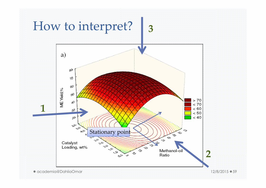
How to interpret?

1

2

3

Stationary pointStationary point


6) Optimization• Single response

• Multi response


Optimization: Single response-Critical value

Will identified the point on the quadratic response surface either it the minimum, maximum, or saddle point of the surface.

The critical values for the independent variables are the coordinates of the origin of the quadratic response surface.

Shown the predicted value of the dependent variable (response) at the critical values for each of the independent variables.


OPTIMIZATION: Multi-response

• Superimpose of two contour plot.


OPTIMIZATION: Multi-response via

Desirability Function

A popular and established technique for simultaneous determization of optimum settings of input variables that can determine optimum performance levels for one or more responses

Converting the estimated response model ( Y) into individual desirability function (d) that are then aggregated into a composite function (D).

This composite function is usually a geometric or an arithmetric , which will be maximized or minimized, respectively.


Desirability Profile

Predicted value

Process variable

Desirability 12/8/2015 64academia@DahliaOmar

3D surface plot


Contour plot


Conclusion DOE and RSM

•A powerful method for design of experimentation, analysis of experimental data, and optimization.

Advantages

• design of experiment, statistical analysis, optimization, and profile of analysis in one step

• Produce empirical mathematical model

Disadvantage

• The prediction only can be determined in range of study.


references


Slide can be found at https://teknologimalaysia.academia.edu/DahliaOmar


Statistica Tutorial 1DESIGN OF EXPERIMENT


DOE spreadsheetOpen spreadsheet STEP 1

Click StatisticaSTEP 2


Click industrial statistics & six Click industrial statistics & six sigma

STEP 3

Click experimental design (DOE)STEP 4


Design & analysis of experiment windows

Click central composite, non factorial, surface Click central composite, non factorial, surface design→ok

STEP 5


Pick suitable design →okSTEP 6

CCD


Click change factor value etcSTEP 7


Change value

Insert the variable and range → okSTEP 8


Click design display Click design display (standard order)

STEP 9

Design display on workbook windows


Copy DOE to spreedsheet

Select all right clickSelect all → right click→copy with headers

STEP 1

Paste on spreadsheetSTEP 2


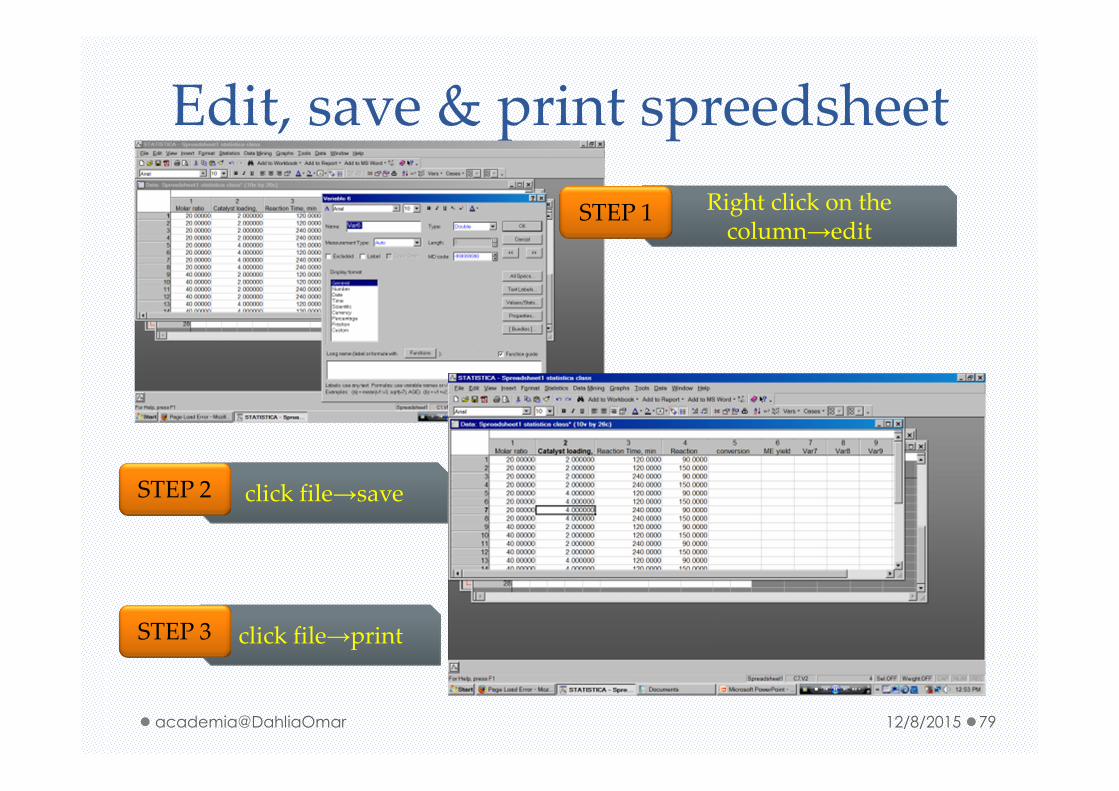
Edit, save & print spreedsheetRight click on the Right click on the

column→editSTEP 1

click file→saveSTEP 2

click file→printSTEP 3


Statistica tutorial 2INSERT AND ANALYSIS THE DATA


Insert the result into spreadsheet

Remember save the spreadsheet(note: spreadsheet is an important in statistica)

Open spreadsheet and insert the result STEP 1


Click StatisticaSTEP 2

Click industrial statistics & six Click industrial statistics & six sigma

STEP 3

Click experimental design (DOE)STEP 4


Click central composite, non factorial, surface Click central composite, non factorial, surface design→ok

STEP 5

Click analyze design tabSTEP 6


Click variablesSTEP 8


Pick variable →okSTEP 9

Click okSTEP 10


Analysis of the central composite (response surface) experiment windows opened.Analysis of the central composite (response surface) experiment windows opened.(note: this windows is an important for analysis since it display all information

needed)


Save as project

Click file → save project asSTEP 11

This statistica project file can be opened anytime and the analysis and workbook could be resume.


STATISTICA TUTORIAL 3PREDICTED/EMPIRICAL MODEL


Model (Coefficient selection)

STEP 1


Click Anova/effect Click Anova/effect →regression coefficient

STEP 2

434232413121

2

4

2

3

2

2

2

143212

005.0001.0056.0011.0004.0198.0

003.0001.0843.0050.0978.1774.0266.0623.4048.192

XXXXXXXXXXXX

XXXXXXXXY

−++−+−

−−−−++−+−=


STATISTICA TUTORIAL 4ANOVA


ANOVA/Effects

Click ANOVA table tabSTEP


ANOVA table

SourcesSum of

Squares(SS)

Degree of

Freedom(d.f)

Mean Squares

(MS)F-value F0.05

Regression

(SSR)2807.32 14 200.52 3.39 >2.74

Residual 649.87 11 59.08

Total (SST) 3457.29 25

R2>0.75 (Haaland, 1989)

SST

Residual

SSR= SST-residual

DF

DFSSR= DFSST-DF residual12/8/2015 93academia@DahliaOmar

STATISTICA TUTORIAL 5Effects


Tab of ANOVA/Effects


Effect estimates


STATISTICA TUTORIAL 6Mean Effect




STATISTICA TUTORIAL 7Contour plot



STATISTICA TUTORIAL 83D Surface



STATISTICA TUTORIAL 9Optimization: Single response


OPTIMIZATION: Single responses

Predicted response

Click quick tab critical value (min, Click quick tab→ critical value (min, max, saddle)

STEP 1


STATISTICA TUTORIAL 10Optimization: Desirability function



Desirability profile

3D surface plot

Contour plot


Documents

Design of experiment and Response surface methodology