DAO O�ce Note 97-05O�ce Note Series onGlobal Modeling and Data AssimilationRichard B. Rood, HeadData Assimilation O�ceGoddard Space Flight CenterGreenbelt, MarylandDesign of the Goddard EarthObserving System (GEOS) ParallelPhysical-space Statistical AnalysisSystem (PSAS)P. M. Lyster�, J. W. Larson�, C. H. Q. Dingz,J. Guoy, W. Sawyer�, A. da Silva, I. �Stajner��Data Assimilation O�ceNASA/Goddard Space Flight Center, Greenbelt, MarylandAdditional A�liations:� Joint Center for Earth System Science (JCESS), University of Marylandy General Sciences Corporation (a subsidiary ofScience Applications International Corporation).��Universities Space Research Association.z National Energy Research Scienti�c Computing Center.This paper has not been published and shouldbe regarded as an Internal Report from DAO.Permission to quote from it should beobtained from the DAO. ��������������������������������������������������������������������������������������������������������������������������������������������������������������������������������������������������������������������������������������������������������������������������������������������������������������������������������������������������������������������������������������������������������������������������������������������������������������������������������������������������������������������Goddard Space Flight CenterGreenbelt, Maryland 20771February 1997

AbstractThe Physical-space Statistical Analysis System (PSAS) comprises the coreanalysis scheme for the Goddard Earth Observing System (GEOS) atmosphericdata assimilation system. The Data Assimilation O�ce (DAO) of the NationalAeronautics and Space Administration (NASA) developed both GEOS andPSAS, and are currently in the process of constructing a parallel implemen-tation of GEOS. Here we discuss the progress in the parallel implementationof PSAS, which has culminated in the construction of the prototype parallelPSAS. This document derives from two week-long workshops that were con-ducted at the NASA/Goddard Space Flight Center Data Assimilation O�ce(DAO) on September 30 to October 4, and October 28 to November 1, 1996.The purposed of these workshops was to review the requirements for the de-velopmental parallel Physical-space Statistical Analysis System (PSAS) and tolay the groundwork for the prototyping and design of the operational PSASthat will be a part of the Goddard Earth Observing System data assimilationsystem GEOS 3.0. This will use the Message Passing Interface (MPI) library,with some heritage C and Fortran 77 code, and with an overarching Fortran 90(f90) modular design.iii

ContentsAbstract iii1 Introduction 12 The Scienti�c Algorithm 23 Requirements 44 The JPL Prototype Parallel PSAS 54.1 Summary of the algorithm . . . . . . . . . . . . . . . . . . . . . . . . 54.1.1 Parallel Partition . . . . . . . . . . . . . . . . . . . . . . . . . 74.1.2 Matrix Block Partition . . . . . . . . . . . . . . . . . . . . . . 84.1.3 Solve Parallel Conjugate Gradient . . . . . . . . . . . . . . . . 104.1.4 Calculate Analysis Increment . . . . . . . . . . . . . . . . . . 104.2 Summary of Timings for PSAS JPL . . . . . . . . . . . . . . . . . . . 115 Developmental PSAS 2.1 and 3.0 135.1 Summary of PSAS 2.1 . . . . . . . . . . . . . . . . . . . . . . . . . . 135.1.1 Parallel Partition . . . . . . . . . . . . . . . . . . . . . . . . . 145.1.2 Matrix Block Partition . . . . . . . . . . . . . . . . . . . . . . 165.1.3 Solve Parallel Conjugate Gradient . . . . . . . . . . . . . . . . 175.1.4 Calculate Analysis Increment . . . . . . . . . . . . . . . . . . 176 The Parallel Evaluation of Forecast Error Covariance Matrices 186.1 PSAS JPL, PSAS 2.1, and PSAS 3.0 . . . . . . . . . . . . . . . . . . 186.2 Issues for Evaluating P f on the Analysis Grid . . . . . . . . . . . . . 187 Optimization and Load Balance 218 Input/Output and the PSAS-GCM Interface 229 Parallel Quality Control 2310 Reproducibility 2311 Portability, Reusability, and Third-Party Software 25Appendix A: List of Symbols and De�nitions 29A.1 List of Symbols . . . . . . . . . . . . . . . . . . . . . . . . . . . . . . . 29A.2 De�nitions . . . . . . . . . . . . . . . . . . . . . . . . . . . . . . . . . 29A.3 Versions of algorithms . . . . . . . . . . . . . . . . . . . . . . . . . . . 30A.4 PSAS JPL Datatypes . . . . . . . . . . . . . . . . . . . . . . . . . . . 30A.5 PSAS 2.1 Datatypes . . . . . . . . . . . . . . . . . . . . . . . . . . . . 31A.6 Data Attributes . . . . . . . . . . . . . . . . . . . . . . . . . . . . . . 31iv

Appendix B: PSAS JPL Data Structures 32B.1: Obs handle Structure . . . . . . . . . . . . . . . . . . . . . . . . . . . 32B.2: Gpt handle Structure . . . . . . . . . . . . . . . . . . . . . . . . . . . 34B.3: Vec handle Structure . . . . . . . . . . . . . . . . . . . . . . . . . . . 35B.4: Grd handle Structure . . . . . . . . . . . . . . . . . . . . . . . . . . . 38B.5: Gvec handle Structure . . . . . . . . . . . . . . . . . . . . . . . . . . 40Appendix C: GEOS 2.1 Data Types 42C.1: Obs Vect Type . . . . . . . . . . . . . . . . . . . . . . . . . . . . . . 42C.2: State Vect Type . . . . . . . . . . . . . . . . . . . . . . . . . . . . . 42C.3: Anal Vec Type . . . . . . . . . . . . . . . . . . . . . . . . . . . . . . 43Appendix D: GEOS 3.0 Proposed Data Types 44D.1: Gpt handle f90 . . . . . . . . . . . . . . . . . . . . . . . . . . . . . . 44Appendix E: Notes on the JPL Parallel PSAS Code 45E1. Where the JPL Parallel PSAS is Archived . . . . . . . . . . . . . . . . 45E.2 About the Source Code for the Parallel PSAS . . . . . . . . . . . . . . 45E.3 Building the Executable JPL Parallel PSAS . . . . . . . . . . . . . . . 46E.4 Running the JPL Parallel PSAS . . . . . . . . . . . . . . . . . . . . . 47E.5 Procedures for Modifying the Source Code . . . . . . . . . . . . . . . . 48E.6 Sample Input Parameter File param.in . . . . . . . . . . . . . . . . . 51Appendix F: Workshop Participants 52Appendix G: Figures 53

v

1 IntroductionThe Physical-space Statistical Analysis (PSAS) algorithm is a signi�cant part of theGEOS atmospheric data assimilation system that is used by the Data AssimilationO�ce (DAO). Apart from the considerable technology surrounding the data I/O,storage, transmission to and from data facilities, and data visualization, the corecomponents of GEOS are an atmospheric general circulation model (GCM), a cou-pler that interpolates the GCM output onto the observation grid and calculates thedi�erence between the forecast and observation (known as innovations), a data qualitycontrol (QC) system that checks these innovations for suspect values, and the analysisscheme PSAS (Figure 1). These are compute-intensive algorithms that, because ofthe nature of the underlying physical models, are highly coupled.The DAO is preparing to move its data assimilation system to advanced comput-ing platforms. This will be part of its regular operation, although an important roleis expected for the Mission to Planet Earth (MTPE) system in the coming years.Key components of the gridpoint-based GCM (Takacs et al. 1996) have been paral-lelized, and are expected to be incorporated into the system in the coming year. In1994, the core components of the developmental serial version of PSAS were takenover by computer scientists at the Jet Propulsion Laboratory (JPL) as part of theHigh Performance Computing and Communications (HPCC) project. The algorithm(PSAS JPL) was parallelized using distributed-memory Single ProgramMultiple Data(SPMD) message-passing approach (Ding and Ferraro 1995).The workshops that are summarized in this document were intended to �rst sum-marize the requirements (Stobie 1996) and to initiate the prototyping and design forthe parallel system GEOS 3.0. It should be noted that the current scienti�c (serial)versions PSAS 2.0 and parallel PSAS JPL have diverged considerably since 1994.This was the result of a conscious decision that was made at the time because it wasknown that the serial code was undergoing considerable scienti�c development andchange. It is our intention to merge the parallel technology with the newest versionPSAS 2.1 and generate the �rst uni�ed parallel algorithm that we designate PSAS3.0. Thereafter the development of parallel code will not diverge from the scienti�cproduction code. In order to plan the message-passing methodology, the approachwe took was to review the JPL parallel code (the �rst week September 30 to October4) and then study the data life cycle in the serial PSAS 2.1 (October 28 to November1). PSAS JPL is written in C (approximately 15; 000 lines of code) that uses theMessage Passing Interface (MPI) library, and calls low-level Fortran 77 subroutines1

(7; 500 lines). We are most interested in how this technology will transfer to theenvironment that is planned for PSAS 2.1, which uses f90 extensively and MPI. Keyissues are the e�ciency of on-processor code and message-passing functions, and theload balancing of the new algorithm. To do this, both the software constructs (f90types) and the physical layout of memory need to be considered; the latter is espe-cially important for RISC-based processors such as the ones the DAO is likely to beusing. The di�cult task of Con�guration Management which will specify the processof merging PSAS JPL with PSAS 2.1 to generate PSAS 3.0 will be left to the GEOS3.0 Design Team.2 The Scienti�c AlgorithmFour Dimensional Data Assimilation (4DDA) is the process whereby a state forecastand observations are combined to form a best estimate, or analysis, of the state (Daley1992). A forecast is derived from a model (e.g., GCM) of the system. The data foran analysis are up to 150; 000 observations over a six hour period. 4DDA may beused to provide the initial conditions for a weather forecast. 4DDA is also used atthe DAO and other institutions to perform reanalyses of past datasets in order toobtain a continuous, gridded, best estimate of the atmosphere for key state variables(e.g., height, wind, surface pressure, and moisture). The DAO also provides supportfor measurement instrument operation. DAO will provide software for an operationalreanalysis 4DDA system by the year 1998 under the Mission to Planet Earth (MTPE).As mentioned in the Introduction, the core compute-intensive components are themodel GCM, the quality control QC, and PSAS. The complexity of the GCM isO(n),where n is the number of gridpoints on the analysis grid multiplied by the number ofstate variables. The analysis takes p observations that are inhomogeneously placedin space and time and through a statistical interpolation modi�es a forecast wf 2 IRnto form an analysis wa 2 IRn. The approach of PSAS (da Silva et al. 1995) solves alarge matrix problem using the following formulation: The innovation equation(HP fHT +R)x = wo �Hwf ; (1)and the analyzed state is given by the analysis equationwa = wf + P fHTx: (2)where wo(2 IRp) is the vector of observations; P f (IRn ! IRn) is the speci�ed forecasterror covariance matrix; R(IRp ! IRp) is the speci�ed observation error covariance2

matrix; H(IRn ! IRp) represents a generalized interpolation from the analysis gridto the observations; and x(2 IRp) is a vector of weights.Multiple observations from an instrument at the same horizontal position arecalled pro�les, i.e., it is assumed for the current development that members of thesame pro�le (e.g., radiosonde or satellite measured radiances) are at the same positionof latitude and longitude. It is convenient to writeH = FI; (3)where I(IRn ! IRs) interpolates from the analysis grid to the state grid which isa grid whose horizontal locations are the locations of pro�les and whose vertical loca-tions are standard levels for a discretized forward operator. (i.e., a quasi-unstructuredgrid). The observation operator F (IRs ! IRp) models wo on the observation grid (anunstructured grid) from the interpolated variables on the state grid. (i.e., F actson individual pro�les on the state grid to produce the corresponding pro�les in theobservation grid). For the current formulation of PSAS, the �rst term HP fHT inthe innovation equation is evaluated as FP fs F T where P fs is the approximation ofIP fIT , evaluated directly on the state grid using speci�ed forecast error variancesand a correlation model. The correlation model is implemented using lookup tableswhose coordinates are the appropriate horizontal and vertical coordinates. For PSASJPL there is no F operator since only state variables are assimilated. One of the keychanges in PSAS 2.1 is the assimilation of non-state variables. For example (Lamichand da Silva 1996) layer thickness, total precipitable water, and cloud-cleared ra-diances will be directly assimilated. In these cases F is the tangent linear forwardmodel and is often obtained from instrument teams.The innovation equation is solved using a preconditioned conjugate gradient al-gorithm (Golub and van Loan 1989, da Silva and Guo 1996). This is an O(Nip2)operation, where Ni is the number of iterations of the CG solver. Typically, betweeneight and twelve iterations are needed to produce a CG solution whose residual hasbeen reduced by at least two orders of magnitude. Experiments in which the residualsare reduced by more than two orders of magnitude resulted in errors in x that muchsmaller than expected analysis errors.while solution of the analysis equation is an O(np) operation.As mentioned earlier, the innovation matrix HP fHT + R is dense, although en-tries associated with locations that are separated by several correlation lengths arenegligible (or zero for compactly supported correlation functions, Gaspari and Cohn1996). In order to introduce some sparseness in HP fHT +R and save computational3

e�ort, the correlations beyond a preset cuto� distance are not included. For PSASJPL, with a 6; 000 kilometer cuto� between centroids of regions the innovation matrixis approximately 26% full, and this uses in excess of 5 gigabytes of storage.3 RequirementsThe scienti�c and software requirements are set out in the document: Data andArchitectural Design for the GEOS 2.1 Data Assimilation System Document Version1 (Lamich and da Silva 1996), and GEOS 3.0 SystemRequirements (Stobie 1996). ForGEOS 3.0 we outline the following requirements that pertain to the parallelizatione�ort:� The parallel PSAS 3.0 will be prototyped and designed along with the serialversion PSAS 2.1. In particular, the code is being developed using f90, and willhandle non-state variable observation operators. The formal merging of theserial and parallel coded will be done in 1997 on a schedule to be determinedby the DAO GEOS 3.0 Design Team.� The parallel design must generate scienti�c software that will have a long lifecycle. The recent development of PSAS as a new algorithm for data assimilation,and the incorporation of f90 into GEOS 2.1 a�ords the opportunity to use amodular approach that allows for expandability, decreases the likelihood of bugs,and makes it easier for a larger group of scientists to use and modify the samecode. It is commonly acknowledged that parallel computing, and message-passing in particular, are su�ciently complex that some e�ort has to be madeto hide the communication modules from a substantial population of the regularprogrammers.� After an extensive review of DAO computing activities, and following the recom-mendation of the external DAO Review Panel (Farrell et al. 1996), theMessagePassing Interface (MPI) parallel library will be used. If necessary, mixed lan-guage third-party software may be used provided portable Fortran bindings areavailable.� The parallel code must scale to meet the performance needs of future productione�orts of the DAO. This includes a commitment to MTPE by 1998 (Zero et al.1996), and ongoing commitments to HPCC (Lyster et al. 1995).4

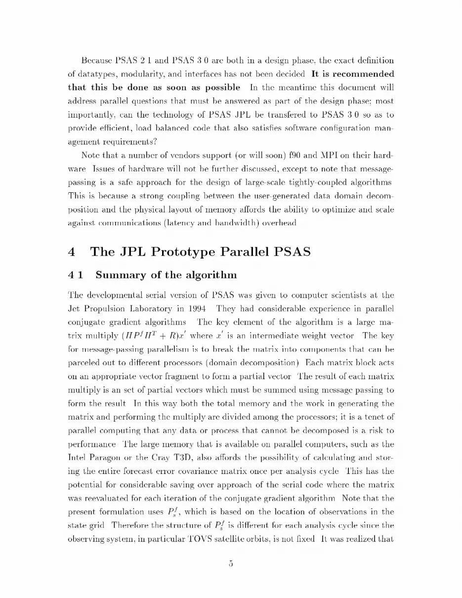
Because PSAS 2.1 and PSAS 3.0 are both in a design phase, the exact de�nitionof datatypes, modularity, and interfaces has not been decided. It is recommendedthat this be done as soon as possible. In the meantime this document willaddress parallel questions that must be answered as part of the design phase; mostimportantly, can the technology of PSAS JPL be transfered to PSAS 3.0 so as toprovide e�cient, load balanced code that also satis�es software con�guration man-agement requirements?Note that a number of vendors support (or will soon) f90 and MPI on their hard-ware. Issues of hardware will not be further discussed, except to note that message-passing is a safe approach for the design of large-scale tightly-coupled algorithms.This is because a strong coupling between the user-generated data domain decom-position and the physical layout of memory a�ords the ability to optimize and scaleagainst communications (latency and bandwidth) overhead.4 The JPL Prototype Parallel PSAS4.1 Summary of the algorithmThe developmental serial version of PSAS was given to computer scientists at theJet Propulsion Laboratory in 1994. They had considerable experience in parallelconjugate gradient algorithms. The key element of the algorithm is a large ma-trix multiply (HP fHT + R)x0 where x0 is an intermediate weight vector. The keyfor message-passing parallelism is to break the matrix into components that can beparceled out to di�erent processors (domain decomposition). Each matrix block actson an appropriate vector fragment to form a partial vector. The result of each matrixmultiply is an set of partial vectors which must be summed using message passing toform the result. In this way both the total memory and the work in generating thematrix and performing the multiply are divided among the processors; it is a tenet ofparallel computing that any data or process that cannot be decomposed is a risk toperformance. The large memory that is available on parallel computers, such as theIntel Paragon or the Cray T3D, also a�ords the possibility of calculating and stor-ing the entire forecast error covariance matrix once per analysis cycle. This has thepotential for considerable saving over approach of the serial code where the matrixwas reevaluated for each iteration of the conjugate gradient algorithm. Note that thepresent formulation uses P fs , which is based on the location of observations in thestate grid. Therefore the structure of P fs is di�erent for each analysis cycle since theobserving system, in particular TOVS satellite orbits, is not �xed. It was realized that5

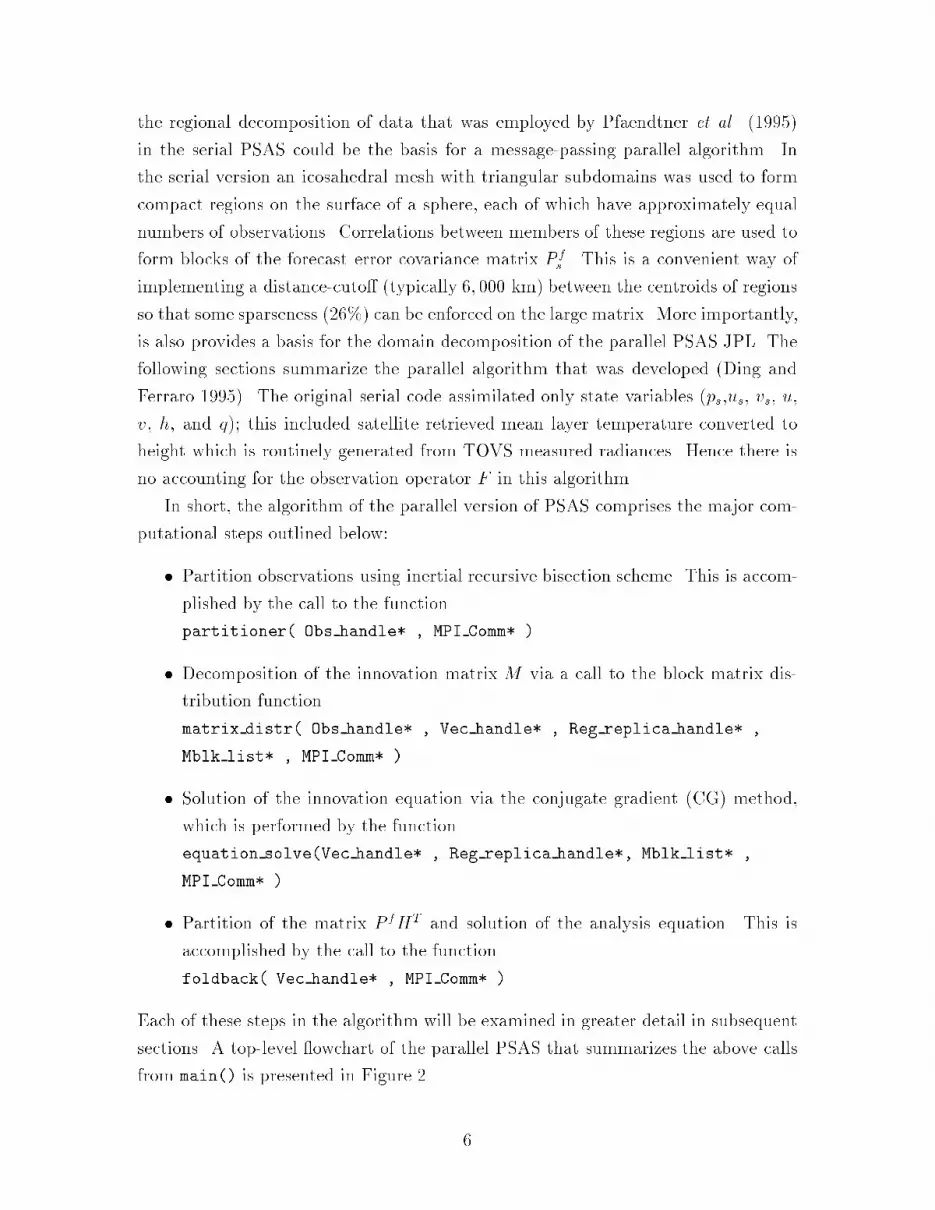
the regional decomposition of data that was employed by Pfaendtner et al. (1995)in the serial PSAS could be the basis for a message-passing parallel algorithm. Inthe serial version an icosahedral mesh with triangular subdomains was used to formcompact regions on the surface of a sphere, each of which have approximately equalnumbers of observations. Correlations between members of these regions are used toform blocks of the forecast error covariance matrix P fs . This is a convenient way ofimplementing a distance-cuto� (typically 6; 000 km) between the centroids of regionsso that some sparseness (26%) can be enforced on the large matrix. More importantly,is also provides a basis for the domain decomposition of the parallel PSAS JPL. Thefollowing sections summarize the parallel algorithm that was developed (Ding andFerraro 1995). The original serial code assimilated only state variables (ps,us, vs, u,v, h, and q); this included satellite retrieved mean layer temperature converted toheight which is routinely generated from TOVS measured radiances. Hence there isno accounting for the observation operator F in this algorithm.In short, the algorithm of the parallel version of PSAS comprises the major com-putational steps outlined below:� Partition observations using inertial recursive bisection scheme. This is accom-plished by the call to the functionpartitioner( Obs handle* , MPI Comm* ).� Decomposition of the innovation matrix M via a call to the block matrix dis-tribution functionmatrix distr( Obs handle* , Vec handle* , Reg replica handle* ,Mblk list* , MPI Comm* )� Solution of the innovation equation via the conjugate gradient (CG) method,which is performed by the functionequation solve(Vec handle* , Reg replica handle*, Mblk list* ,MPI Comm* )� Partition of the matrix P fHT and solution of the analysis equation. This isaccomplished by the call to the functionfoldback( Vec handle* , MPI Comm* ).Each of these steps in the algorithm will be examined in greater detail in subsequentsections. A top-level owchart of the parallel PSAS that summarizes the above callsfrom main() is presented in Figure 2. 6

4.1.1 Parallel PartitionThis algorithm divides p observations among Nr regions using bisection on the sur-face of a sphere. The data are read in as innovations (wo � Hwf ) and distributedin random order (but in equal numbers) on Np processors. In the �rst iteration, theobservations are divided along the orthogonal cut of their combined principal axismoment of inertia. Successive iterations are performed in a tree structure that re-peats the decomposition on half the remaining processors with approximately halfthe data. At each stage, the calculation of the principal axis is performed in parallel.As regions replicate, data are moved between di�erent processors using split MPIcommunicators. The inertial division guarantees some degree of compactness of theresulting decomposition. This algorithm requires there to be power-of-two numberof processors and number of regions, with Nr � Np. Typically, Np = 256, or 512,and Nr = 512. It is possible to modify the power-of-two restriction on numbers ofregions and processors (the orthogonal cut may be made anywhere along the principalaxis to give a division of observations other than 50-50), and maintain approximatelyequal numbers of observations per region. However if the number of regions in eachprocessor is not �xed for all processors there may be some load imbalance in the anal-ysis equation (section 5.1.4). A schematic for the parallel partition of observationsis shown in Figure 1. Note that the decomposition is in terms of equal numbers ofobservations, and that the regions are not necessarily equal in area. Also, the de-composition is two dimensional and pro�les are not permitted to be divided betweenregions (for reasons that will be discussed in section 5.1.2).The key structures (C) for the parallel partition are shown in Appendix B.1(Obs_handle) and B.2 (Gpt_handle). Initially, the unsorted observations are approx-imately equally distributed among processors. The structure Obs_handle referenceselemental structures of type Observ that store the observations (actually innovations,wo�Hwf ) del, and a number of attributes (id, kt, kx, rlats, rlons, rlevs, xyz[3],SigO, and sigF). The allocated memory for all the observations on each processoris contiguous. The structure Gpt_handle (not to be confused with gridpoints of aregular grid) is very similar to Obs_handle except that the elemental type (Gpoint)holds only the coord positions of the observations on a unit sphere, a sequencingid, and the original processor orgn_proc (numbered from 0 to Np � 1) where eachobservation is initially located. Using Gpt_handle the parallel partitioner proceedsby only passing data of type Gpoint between processors. In this way minimal dataare passed (i.e., the other attributes and the value aren't passed during successivebisections of the the parallel partitioner). At each bisection, each processor identi�es7

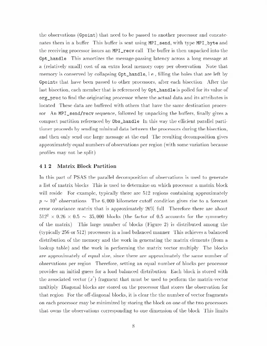
the observations (Gpoint) that need to be passed to another processor and concate-nates them in a bu�er. This bu�er is sent using MPI_send, with type MPI_byte andthe receiving processor issues an MPI_recv call. The bu�er is then unpacked into theGpt_handle. This amortizes the message-passing latency across a long message ata (relatively small) cost of an extra local memory copy per observation. Note thatmemory is conserved by collapsing Gpt_handle, i.e., �lling the holes that are left byGpoints that have been passed to other processors, after each bisection. After thelast bisection, each member that is referenced by Gpt_handle is polled for its value oforg_proc to �nd the originating processor where the actual data and its attributes islocated. These data are bu�ered with others that have the same destination proces-sor. An MPI_send/recv sequence, followed by unpacking the bu�ers, �nally gives acompact partition referenced by Obs_handle. In this way the e�cient parallel parti-tioner proceeds by sending minimal data between the processors during the bisection,and then only send one large message at the end. The resulting decomposition givesapproximately equal numbers of observations per region (with some variation becausepro�les may not be split).4.1.2 Matrix Block PartitionIn this part of PSAS the parallel decomposition of observations is used to generatea list of matrix blocks. This is used to determine on which processor a matrix blockwill reside. For example, typically there are 512 regions containing approximatelyp � 105 observations. The 6; 000 kilometer cuto� condition gives rise to a forecasterror covariance matrix that is approximately 26% full. Therefore there are about5122 � 0:26 � 0:5 � 35; 000 blocks (the factor of 0:5 accounts for the symmetryof the matrix). This large number of blocks (Figure 2) is distributed among the(typically 256 or 512) processors in a load balanced manner. This achieves a balanceddistribution of the memory and the work in generating the matrix elements (from alookup table) and the work in performing the matrix vector multiply. The blocksare approximately of equal size, since there are approximately the same number ofobservations per region. Therefore, setting an equal number of blocks per processorprovides an initial guess for a load balanced distribution. Each block is stored withthe associated vector (x0) fragment that must be used to perform the matrix-vectormultiply. Diagonal blocks are stored on the processor that stores the observation forthat region. For the o�-diagonal blocks, it is clear the the number of vector fragmentson each processor may be minimized by storing the block on one of the two processorsthat owns the observations corresponding to one dimension of the block. This limits8

the ability to simply parcel out the blocks in a deterministic and load-balanced way.From the initial state, the load-balancing scheme proceeds towards this goal by �rstre�ning the initial distribution to produce a new initial state using the followingscheme:1. The load on each processor Li to perform work for the conjugate gradient solveris estimated, along with the average load �L. This leads to a set of imbalances�i � �L� Li2. For each pair (i; j) of processors, an exchange probability Pij = LjLi+Lj is calcu-lated.3. Use a random number r 2 [0; 1] to decide if processor i or processor j is assignedthe block. Processor i is assigned the block if r � Pi, while processor j isassigned the block if r > Pi. This amounts to a weighted coin toss.From this re�ned initial state, the block distribution is improved iteratively throughthe following adjustment process:1. For iteration m � Niter, for each pair (i; j) of processors deviations from theaverage load balance �i and �j are calculated, along with the exchange prob-ability Pij described above. The number of blocks on each processor, Ni andNj, respectively, are counted along with the average number of blocks on eachprocessor �N .2. If �i > 0 and �j < 0, the block is transferred from processor i to processor j.If �i < 0 and �j > 0, the block is transferred from processor j to processor i.3. If both �i and �j have the same sign, then if Ni �Nj > �� �N , then the blockis moved from processor i to processor j.4. Finally, for all other cases not covered above, the block is assigned to a processorbased on the weighted coin toss described in the re�nement of the initial state.Following this scheme for Niter = 10 and � = 1=20 results in a load imbalance ofapproximately 10%. The messages that must be exchanged during the matrix blockpartition are matrix indices and geometrical data. No complex structures, such as inthe parallel partition, are exchanged until the block partition is complete.9

4.1.3 Solve Parallel Conjugate GradientThe conjugate gradient algorithm uses block preconditioning, and is described inGolub and van Loan (1989) and da Silva and Guo (1996). Computationally, the coreis the large matrix-vector multiply. In the parallel partitioner the innovations areseparated into regions that are distributed among the processors. These provide theinitial condition for the vector iterate (x0). The vector is actually composed of vectorfragments. The nature of distributed-memory parallel processing is that matrices andvectors are rarely represented as a whole on any one processor (an exception is some-times made for the purpose of performing I/O). Depending on how the o�-diagonalblocks are distributed, some of these vector fragments must be replicated on multipleprocessors. Furthermore the algorithm that generates the blocks uses lookup tableswith inner loops over same-data types. Hence the vectors are reordered and referencedby a third structure Vec_handle (Appendix B.3). This is similar to the previously de-scribed structures except that the elemental type Vec_region references long vectorsof attributes and data. In this case message-passing is easy since the same datatypesare e�ectively already bu�ered. It may be possible to sum the partial vectors usingMPI split communicators and the MPI_reduce(...,MPI_sum,...) function. Thisuses a butter y-tree algorithm. It turns out that the hand written code optimizedusing MPI_send/recv functions is more e�cient since the number of processors hold-ing any particular vector segment is small compared to the total number of processingunits (C. Ding personal communication).For PSAS JPL an older, considerably less e�cient algorithm was used to performthe table lookup (it has been made faster in the present development PSAS by anorder of magnitude). Hence, the generation of the matrix elements was a dominantpart of the cost. The savings in evaluating the matrix only once per analysis cyclewas considerable; e�ectively Ni (the number of CG iterations) multiplied by the costof generating the matrix.4.1.4 Calculate Analysis IncrementThe analysis increment is (Eq. 2) P fHTx. The operator P fHT � P fIT repre-sents the forecast error covariance between the observation grid and the analysisgrid. The domain decomposition for this must account for the unstructured dis-tribution of the observations and the structured analysis grid. The solution vectorx for the conjugate gradient algorithm is decomposed in the same manner as theobservations (Section 4.1.1). The decomposition for the analysis grid is based on10

the fact that gridpoints within the 6; 000 mile cuto� of the location of an obser-vation are a�ected by the corresponding weight in the vector x. A deterministicload-balanced algorithm proceeds as follows: an equal area rectangular distributionof gridpoints is generated (Figure 3). The boundaries of these regions are along lati-tude and longitude coordinate axes. At higher latitude the boundaries of the regionsin the latitude-longitude plane is altered to keep the area in each region �xed, witha single cap over the poles. The gridpoints in these equal-area regions are thinnedlongitudinally; this is also performed increasingly with higher latitude in such a waythat the number of gridpoints in each equal area region is the same. In this man-ner the matrix P fHT may be generated as a number of equal-sized blocks whosecentroids are within the 6; 000 km cuto� distance of the centroids of each region ofx. Since there is a �xed number of regions per processor (i.e., usually 1 or 2) thenumber and size of the corresponding matrix blocks and the work that is performedin the partial matrix-vector multiply is the same on all processors. The structuresthat are used in this are Grd_handle and Gvec_handle these have the property thatthey are pointers to pointers, and are dereferenced at the lowest level of the call-ing tree in the foldback process, create gvec regions(grd handle, gvec handle)and analysis inc(vec handle, gvec handle, grd handle). The partial vectorsare then combined by using MPI All reduceCP.4.2 Summary of Timings for PSAS JPLTable 1. shows the timing for PSAS JPL for 80; 000 observations (model resolution2:5o�2o�14 levels) on 512 processors of the Intel Paragon at the California Instituteof Technology. The solver achieves 18:3 giga op/s (77 mega op/s per processor),which is 36% of peak performance for 512 processors. The parallel partitioner takes3:1 seconds. This is a relatively small cost; the communications are complex butbecause of the strategy of sending minimal data and bu�ering there is little overhead.The calculation of block distribution lists uses a small amount of communications topass simple lists between processors. During the replication of observation regions,vector fragments referenced by Vec_handle are sent between processors. These arerelatively long messages and have little overhead. The calculation of matrix entriesis very time consuming (23:8 seconds), but is performed only once per analysis. Thesolver uses BLAS level 2 library calls (sgemv) and messages (MPI SEND and MPI RECV)to send vector fragments of x0. This is iterated Ni � 100 times 1, taking 36:4 seconds.1This number of iterations di�ers from the value of Ni cited earlier because the version of PSASthat was parallelized had a more stringent convergence criterion than subsequent versions of PSAS.11

The dominant cost of the analysis equation (referred to in Ding and Ferraro (1995)as \fold back") is from the generation of the matrix elements. Since one dimension ofP fHT is n which is larger than p this takes longer than the generation of the innova-tion matrix. The communication (1:5 seconds) involved in reassembling the analysisgrid vector is similar to the assembly of vector fragments in the innovation equation.For the innovation equation:Task Time(sec)Read input data 14.6Partition observations 3.1Calculate block distribution lists 3.8Replicate observation regions 3.3Calculate matrix entries 23.8Solve parallel CG 36.4Miscellaneous 1.7Total 87.0Secondly, for the analysis equation:Task Time(sec)Create grid partition 0.4Assemble and evaluate P fHTx 67.6Reassemble model vector 1.5Total 69.5Table 1. Timings for PSAS JPL on the 512 processor Intel Paragon at the CaliforniaInstitute of Technology.The op rates for runs that were recently performed on the Cray T3D at theNASA/Goddard Space Flight Center are shown in Figure 4. The closed circles arefor a problem with 51; 990 observations and the diamonds are for 79; 938 observations.Version solve conj grad. analysis equation1994 PSAS 9120. (sec) 9000.1996 PSAS 750. 750.PSAS JPL 87. 71.As was mentioned earlier, the condition cited here is more stringent than was later learned to benecessary. 12

Table 2. Comparison of timings for two versions of the serial PSAS and parallel PSASJPL.Table 2 shows a comparison between wall-clock times for three versions of PSAS:the serial code that was given to JPL as run on a single processor Cray C90; a recentoptimized serial PSAS also run on a Cray C90; and a PSAS JPL run on 512 processorof the Intel Paragon. The older serial code is slower than JPL PSAS by two orders ofmagnitude, mainly due to the higher net op rate of the parallel processor (approxi-mately 10 giga op/s to 1 giga op/s) and the calculation of the matrix elements onlyonce per conjugate gradient solve. The more recent, optimized, PSAS runs faster onthe C90 because the algorithm for table lookup has been improved (making more useof redundancy and using nearest-neighbor lookup). In the future the need to formthe error covariance matrices only once may be relaxed. This is discussed further insection 7.5 Developmental PSAS 2.1 and 3.05.1 Summary of PSAS 2.1The developmental serial PSAS 2.1 di�ers from older versions in two main ways: theuse of f90 modules and types to modernize the software; and the incorporation ofobservation operators. Fortran 90 may impact message-passing through changes inthe way observations are bu�ered in the parallel partitioner and vectors are passedin the replication and solve subroutines. Fortran 90 may also a�ect single-processorperformance if pointers are not used carefully. PSAS 3.0 is the parallel version, andthis paper deals mostly with the special problems associated with its development.The observation operator signi�cantly changes the algorithm (Lamich and da Silva1996). The left hand side of the innovation equation becomes (FP fs F T +R)x, whereF is the tangent linear observation operator. The forecast error covariance matrixis formulated in state space (in particular P fs is dimensioned on the unstructuredstate grid of observation pro�les). This gives rise a new representation of data ona state grid (section 2). Appendix C shows prototypes of f90 types Obs_Vect andState_Vect. Both of these types are built around (unbreakable) pro�les. Attributesthat do not vary along a pro�le are aggregated into types Obs_Att and State_Att.The Obs_Vect has all the attributes that facilitate the quality control functions andthe generation of the F and R operators. The State_Vect has only those attributesthat are needed to generate the forecast error covariance matrices (in particular, the13

quality control qc, metadata index km, sounding index ks are left out, and the posi-tions of the pro�les on the unit sphere xyz are included). The observation operatorsact on pro�les (or aggregates of pro�les { soundings { at the same location). Hence themanner in which the Obs_Vector pro�les are sorted in memory is not that importantto performance. The observation error covariance matrix R may couple soundings,so it may be necessary to co-locate soundings in memory. At the lowest subroutinelevel, the P fa operator is generated using loops over of pairs of locations of pro�les,each dimension of which corresponds to the same variable. Hence it is important tosort State_Vect in memory by data type (kt). The f90 types that are used, such asState_Vect or Obs_Vect actually reference allocated memory space (a memory han-dler). In general, it is the location of variables in memory that a�ects performance. Ifmembers of pro�les or vectors are not appropriately sorted in memory then the innerloops may have to dereference f90 pointers and there may be a performance degra-dation. These are issues that a�ect both a serial and parallel application { especiallyon RISC-based processors (i.e., most scienti�c computers). The following sectionssummarize other aspects of the new data types, and how they may a�ect messagepassing. A summary of performance aspects is given in section 8.5.1.1 Parallel PartitionThis section compares the parallel approach of PSAS 3.0 that uses f90 datatypes incomparison with the approach of PSAS JPL that uses the C language and structures.As discussed in the previous section PSAS JPL uses Gpt_handle and Obs_handlestructures in the parallel partition. Gpt_handle has reduced data (xyz position onthe unit sphere and the identifying number of the originating processor) that allowsthe successive bifurcations of the partition to proceed e�ciently. Is is su�cient hereto show the analogous approach that uses f90 datatypes, and to indicate how this willgive comparable performance. Considerable prototyping will have to be done in thefuture.The type Gpt_holder_f90 that is de�ned in Appendix D performs the equivalentfunction as Gpt_handle. The usage is:type(Gpt_holder_f90) gpt!There are numRegs regions in the problemgpt%numRegs = numRegsallocate(gpt%gpt_region(1:numRegs))do index = 1,numRegs 14

gpt%gpt_region(index)%numGpts=numgpts(index)allocate(gpt%gpt_region(index)%gpoints(1:numgpts(index))do iobs=1,numgpts(indexgpt%gpt_region(index)%gpoints(iobs)%coord(1)=...x position of obs..! ...these data are derived from Obs_Vect...enddoenddoThe parallel partition proceeds in the same way as PSAS JPL. At each stage, asubset of the data of type Gpoint_f90 are bu�ered and passed between processors.There are (at least) two ways to do this:(i) The data that are selected to be communicated are extracted from the holder gptand inserted into two bu�ers of type real (for xyz positions) and integer (fororgn_proc and id). The bu�ers are communicated and unpacked at the recieve-ing processor. This is guaranteed to work since it respects the language types,but the loops that perform the bu�ering are clumsy and perhaps ine�cient.(ii) Allocate a bu�er that stores a periodic array of type Gpoint_f90:type Gpt_buffertype(Gpoint_f90),pointer::p(:)end type Gpt_buffertype(Gpt_buffer) gpt_bufallocate(gpt_buf%p(1:max_obs_buffer))This bu�er can be directly �lled with the data that needs to be passed betweenprocessors. The message will use the formMPI_send(gpt_buf,npoints*size(Gpoint_f90),MPI_BYTE,...).This has been prototyped, and shown to work for the f90 compiler with MPIlibrary on a DEC multiprocessor. However it may not be portable since f90may not always interpret a subroutine argument as a simple pointer to a blockof memory (Hennecke 1996).In Section 4 it was shown how the structure Obs_handle references data withall the attributes sequentially located in memory with each observation value. Inthe last step of the parallel partitioner the identifying numbers of the originating15

processors are used to bu�er the observations and their attributes and send them totheir destination processors. On the other hand, the type Obs_Vect that is shown inAppendix C.1 stores pro�les sequentially. Redundant attributes for each pro�le arestored once per pro�le in the type Obs_Att. The bisection process generates a typeGpt_holder_f90 that speci�es the originating processor for the actual data. If thedata are at least sorted into pro�les before the parallel partition then entire pro�lesand attributes from Obs_Vectmay be bu�ered and sent to the destination processor.This eliminates the need to send unnecessary attributes, and eliminates the need forequivalent structure to Obs_handle where all observations are treated as separateatomic units (along with attributes). Hence, Obs_Vector may ful�ll a role in bothmessage passing and in generating the R and F operators. This indicates that thef90 types Gpt_holder_f90 and Obs_Vect may be used to perform the same functionin the message-passing f90 parallel partitioner as the C structures Gpt_handle andObs_handle do in PSAS JPL.5.1.2 Matrix Block PartitionPSAS 2.1 includes, for the �rst time, the tangent linear observation operator F . Atthe end of the parallel partition, the observations are decomposed in pro�les that arereferenced by Obs_Vect. After that, the adjoint of the observation operator is usedto form F Tx, which is referenced by State_Vect. This is an embarrassingly parallelcalculation since operators F=F T transform pro�les of the observation grid (2 IRp)into pro�les of the state grid (2 IRs). Therefore the forward model and its adjoint donot need to be parallelized { a blessing since they may be dusty-deck serial code { itis mainly for this reason that pro�les are not permitted to be broken in the parallelpartitioner (section 4.1.1 and 5.1.1). For the subsequent evaluation of P fs F Tx thereis a choice of maintaining a decomposition that has approximately equal numbersof observations in each region or transforming to another representation where equalnumbers of the state grid values are in each region. The latter more closely resemblesthe approach of PSAS JPL because the resulting blocks of P fs are approximately ofequal size. The parallel partitioner of PSAS JPL initially assumes that all blocks of theinnovation matrix are the same size (i.e., they cost the same to generate the block andperform the submatrix-vector multiply). The subsequent iterative process, wherebyload-balance is ensured, uses the size of the block as a cost function. Therefore, ifwe use an approximately even decomposition of the state grid the subsequent loadbalance algorithm will be the same as PSAS JPL. For example, the convergence ofthe load-balance calcualation would be as rapid, and the extent of load balance would16

be expected to be the same (PSAS JPL achieves about 10% load balance after 10iterations of the balancing process). The load balance of the operation Fx is notnecessarily assured in this algorithm. However, since the number of pro�les � 104is much larger then the number of processors there would be a natural convergencetoward load balance due to the large numbers. Also, six hours of TOVS soundings(20; 000 pro�les, each of which has 20 channels) takes 5 minutes of processing for theradiative transfer calculation on a 50 mega op/s DEC uniprocessor (J. Joiner, privatecommunication). Therefore, at 10 giga op/s the calculation should take about 1:5seconds which is considerably less than the cost of generation of P fs and the matrix-vector multiply (Table 1). If necessary, the operators corresponding to di�erent typesof pro�les could be costed and the result used to modify the cost function for theevaluation and use of blocks P fs (i.e., use a more sophisticated cost function otherthan the size of the blocks).Note that the operation Rx is performed in the decomposition of the observationgrid. It may be necessary to sort Obs_vect by sounding in order to preserve in-memory locality. This may help performance in a RISC-based processor. Other thanthat, Rx is load balanced and should not require fundamental changes between PSASJPL and PSAS 3.0.5.1.3 Solve Parallel Conjugate GradientFor PSAS 3.0, the conjugate gradient algorithm is not signi�cantly di�erent thanPSAS JPL. The algorithms for replication of fragments of State_Vect and the sub-sequent parallel sum of partial vectors uses values that are sorted into long vectors ofthe same type. This is the same as PSAS JPL which used the structure Vect_handle.5.1.4 Calculate Analysis IncrementThe message-passing that is required to calculate P fs F Tx is similar to PSAS JPL.Matrix block lists and long vectors need to be replicated and passed as necessary.Once again load balance may be an issue. As discussed in section 5.1.2, becauseof the large number of pro�les and the relatively small cost, the load balance forF Tx may not depend on whether x is decomposed in terms of equal number of theObs_Vect or State_Vect. However to ensure load balance of the subsequent matrixgeneration and matrix-vector multiply, the vector F Tx (of type State_Vect) shouldbe decomposed into equal numbers in regions. In this case PSAS 3.0 can use thesame decomposition of the analysis grid Anal_Vect as PSAS JPL (Figure 3). Thiswill guarantee that blocks of P fs are of equal size and there will be the same number17

on all processors. The decomposition is load balanced and static (there is no iterativeload-balancing process here). This may be a problem if we relax the restriction ofequal sized regions and equal number of regions on each processor, because the sizeand number of matrix blocks assigned to processors may become disparate.6 The Parallel Evaluation of Forecast Error Co-variance Matrices6.1 PSAS JPL, PSAS 2.1, and PSAS 3.0One of the advantages of parallel computing is that the memory scales proportionallywith the number of processors (subject to cost) and may allow for the storage of theentire forecast error covariance matrix. As described in section 4.2, if the matrix isstored once there is a time saving proportional to the number of iterations of theconjugate gradient solver Ni. This explains in part the impressive improvement inwall-clock time between the serial PSAS in 1994 and the parallel PSAS JPL (Table 2).Table 2 also shows how the serial algorithm has been made an order of magnitude moree�cient through improved algorithms for calculating the matrix elements. Howeverthere is still some saving in calculating the elements once. For a machine whichis memory de�cient it may be necessary to develop an algorithm that dynamicallydecides whether to store or recalculate matrix elements. The error covariance operatorP fs is not evaluated as a single matrix for current serial versions of PSAS, but isinstead a series of sparse operators that act successively on a vector (A. M. da Silva,Personal Communication). Thus, it is not a matrix that is stored, but rather astructure of coe�cients. This may make it di�cult to evaluate a cost function for theload balancing algorithm, although the large numbers of pro�les per processor shouldameliorate the problem.Currently, for an isotropic and separable formulation of the correlation function,the lookup tables may be stored in memory on each processor. However, as we relaxthese assumptions the lookup tables will grow (possibly up to the size of P f ) and mayhave to be decomposed in a similar way as the matrix blocks (section 4.1.2). Thenext section discusses a related implementation.6.2 Issues for Evaluating P f on the Analysis GridEvaluation of a forecast error covariance matrix is a computationally intensive part ofsolving the innovation and analysis equations. The amount of computation required18

for brute-force evaluation of a general forecast error covariance matrix followed by thematrix-vector multiplication is proportional to the dimensions of the matrix. There-fore, in the current PSAS, the forecast error covariance matrix is evaluated directly onthe state grid instead on the larger analysis grid. We propose an e�cient algorithmwhich applies to a wide class of forecast error correlation functions. The algorithmuses symmetries of the analysis grid to greatly reduce the number of correlation func-tion evaluations over brute-force methods.In the current PSAS, the product of matrices IP fIT , where P f is the n�n and I iss�nmatrix, is approximated by the s�smatrix P fs , where s is typically smaller thann by an order of magnitude. Generally, brute-force evaluation of a full k� k forecasterror covariance matrix requires (k2 + k)=2 covariance function evaluations. Brute-force matrix-vector multiplication requires k2 multiplications and k2 � k additions.In the future, the number of observations p will increase, thus increasing s, as well.If s becomes larger than n, and the interpolation matrix I is implemented as a verysparse matrix, it will be more e�cient to use IP fIT instead of P fs .For a wide class of forecast error covariance functions, the use of IP fIT , withthe algorithm for evaluation of P f presented below, is computationally e�cient evenif the analysis grid is re�ned so that n remains an order of magnitude larger thans. Denote the multidimensional (i.e., multi-level) random �eld of geopotential heightforecast errors by h(p) = fh1(p); h2(p); : : : ; hm(p)g; (4)where h1(p); h2(p); : : : ; hm(p) are random �elds on the sphere (Earth's surface) ofgeopotential height forecast errors corresponding to pressure levels 1; 2; : : : ;m. Thecovariance of h(p) is given by the matrix of covariance functions�(p1;p2) = fBjk(p1;p2)g; (5)and the correlation of h(p) is given by the matrix of correlation functions�(p1;p2) = ( Bjk(p1;p2)Bjj(p1;p1) 12Bkk(p2;p2) 12 ); (6)where Bjk is a covariance function of the random �elds hj and hk, j; k = 1; 2; : : : ;m.The algorithm we propose applies to models where � depends only on parameterswhich are preserved under the symmetries of the uniform longitude-latitude grid onthe sphere. For instance the distance d(p1;p2) (7)19

between p1 and p2 and the absolute value of the latitudesj'1j and j'2j (8)of p1 and p2 are preserved under rotations and re ections of the uniform longitude-latitude grid on the sphere (cf. De�nitions 2.4 and 2.5, Gaspari and Cohn 1996). Thecorrelation � currently used in the PSAS depends only on d(p1;p2).The covariance matrix P f , which is the analysis grid evaluation of multi-levelcovariances between all the state variables (h, u, v, q, ps us and vs) can be written asa product of a diagonal matrix D of standard deviations, and a correlation matrix CP f = DCD: (9)Denote by Chh the block of C of geopotential height forecast error covariances, i.e.,the evaluation of � on the analysis grid. Denote by Chh(j; k; '1; '2) the block of Chhwhich is the evaluation of Bjk between the points on circle of latitude '1 and thepoints on circle of latitude '2. It is assumed that the points on each circle are sortedwith increasing longitude. Denote the number of points on each circle of constantlatitude by I. In the current PSAS, I = 144. If � depends only on the parameters (7)and (8), due to the symmetries of the analysis grid, the matrix Chh has the followingstructure. Each of the blocks Chh(j; k; '1; '2) is a symmetric circulant matrix (seeFigure 7), so there are 2I elements with identical values. Moreover, there are threemore blocks of Chh identical with Chh(j; k; '1; '2),Chh(j; k; '1; '2)= Chh(j; k;�'1;�'2)= Chh(k; j; '2; '1) (10)= Chh(k; j;�'2;�'1):Therefore, there are 8I identical elements of the matrix Chh.The following is a brief description of the algorithm for evaluation of Chh andcomputation of the matrix-vector product zh = Chhyh, which exploits the fact that8I elements of Chh are identical. For every set of 8I identical matrix elements ofChh, their value is computed by one evaluation of the correlation function. These8I matrix elements are needed in computation of some, typically 8I, coordinates ofthe product vector zh. All these coordinates of zh are updated, that is the productof the element of of Chh with a coordinate of yh is added to the previous value of acoordinate of zh. This process is repeated until zh is computed. A sequential version20

of this algorithm was implemented on Cray C-98. It was up to 42 times faster thanthe algorithm which was evaluating every element of the correlation matrix.A parallel version of this algorithm has been implemented in FORTRAN 77 usingMPI on the Cray T3D. The processors are organized in a three-dimensional virtualtopology. The distribution of the work was done in a \card shu�ing" manner, thatis each processor works with every nth circle of constant latitude and pressure level,where n depends on the number of available processors. This distribution of the workhas the property that increasing the support of the correlation function or re�ning thegrid results in a more balanced load. On a grid with 8 levels and meshes of 2 degreesin latitude and 2.5 degrees in longitude using a correlation function with support of3000 km, the speedup of this algorithm was 75.5 on 128 processors.In this algorithm only one value of 8I identical matrix elements is stored at onetime. The algorithm can be modi�ed so that an I� I matrix block Chh(p1; p2; '1; '2)(equal to three other blocks of Chh in equation (10)) is evaluated and stored. Thematrix-vector multiplication of this block with four subvectors of yh can be performedusing a BLAS routine.This algorithm was described for the block Chh of C for simplicity. If correlationfunctions between state variables are modeled by the functions which are currentlyused in the PSAS, the same algorithm applies to evaluation of the the entire matrixC and matrix-vector multiplication z = Cy.7 Optimization and Load BalanceFor message-passing optimization the messages should be few and bu�ered. For thealgorithm that involves communicating lists and information about geometry there aresu�ciently few bytes that this is not a signi�cant burden. For the communication ofvector fragments the data are already e�ectively bu�ered in vectors. Ding and Ferraro(1995) have developed a sophisticated algorithm that optimizes the accumulation ofpartial sums without using the MPI_reduce function. For the communication ofobservation and pro�le data Ding and Ferraro also bu�er data and thus amortize thestartup cost of messages.For RISC-based technology the on-processor optimization performance dependson the ability to move data e�ciently through cache to the arithmetic units and thenback to memory. The process of calculating a covariance matrix and using BLAScalls is, in a sense, optimizing cache because the matrix is an optimal form for theinput data. For cases where C or f90 pointers are used to refer to data, they should21

be dereferenced outside of inner loops. The quantities Rx and F Tx are calculatedone pro�le (or sounding) at a time. P fs (F Tx) is calculated using BLAS functions.F (P fs F Tx) is calculated one pro�le (or sounding) at a time. The evaluation of matrixelements, which is a signi�cant cost, may require prototyping and cache optimization.In particular, indirection is a major problem for cache optimization. For example,modern RISC-based processors may have up to two orders of magnitude di�erencebetween the time it takes to access data in cache (cache is usually kilobytes in size)and the time to access remote data in physical memory. It is often more e�cientto separately sort data and thus avoid indirection on inner loops. For example, forisotropic horizontal correlation functions it may be useful to sort the pro�le pairs inorder of increasing distance before indexing the lookup table in a loop.The load-balancing algorithm of Ding and Ferraro was very successful. We haveshown in section 5.1.2 that for PSAS 2.1 and PSAS 3.0 with observation operatorsthere is no conceptual di�culty with following the same approach. However, theanalysis equation may create problems because it is not self adjusting; it relies on thefact that blocks of P fs on each processor in the folding-back decomposition (Figure3) are the same size and cost. This would be di�cult to maintain if we broke therequirement of having the same number of regions of observations on each processor.8 Input/Output and the PSAS-GCM InterfaceThe calculation of the innovation requires transformation from the analysis grid onwhich the forecast is generated and an observation grid. In principle this is not anexcessive cost in terms of message-passing because the model grid which has p � 106variables (i.e., � 107 bytes) would take approximately 0:1 seconds to be arbitrarilytransformed on a parallel computer with a net bandwidth of � 100 megabytes/s (theseback of the envelope calculations always represent an underestimate because of thehidden cost of message latency). The di�culty is one of writing e�cient, modularsoftware that transforms data between the structured analysis grid (it may be thedomain decomposition of the GCM) and the unstructured observation grid. Similarly,on the back end of PSAS e�cient software needs to be developed for transformingbetween the domain decomposition for the analysis grid of PSAS and that of theGCM. Writing the analysis grid or observation data streams (ODS, da Silva andRedder 1995) to disc using, say, MPI-IO will also need these grid transformationtools. It will be so easy to get beaked to death by a thousand ducks.22

9 Parallel Quality ControlThe present on-line quality control is a two-stage process (Seablom et al., 1991). Thegross check compares innovations (wo �Hwf ) against a speci�ed upper bound. Forany even distribution of pro�les on processors, such as given by the parallel partition(section 4.1.1) the gross check is obviously load-balanced and embarrassingly paral-lel. Those observations that fail the gross check are agged and a subsequent buddycheck is performed. This involves comparing the suspect value with a statisticallyinterpolated estimate based on a number of nearest-neighbor un agged observations.The comparison amounts to data indirection with its concomitant cache ine�ciency.Unless a signi�cant number of observations are agged it is probably not e�cient tosort the data for buddy check. E�ciency is further complicated by a dependency inthe comparison loop that allows re-accepted data to in uence not-yet-buddy-checkeddata. The parallel quality control algorithm of von Laszewski (1996) uses a domaindecomposition based on the analysis grid. Clearly, it makes more sense to use theparallel partition of observations (section 4.1.1) as a basis for the quality control inPSAS 3.0, in e�ect leveraging the work that is already done for the domain decompo-sition of PSAS. Overlap regions of redundant data are used to parallelize the loop forthe buddy check. Because of the redundancy, some processors have to wait for othersto complete their fragment of the buddy-check loop, thus giving rise to a potentiallypathological load imbalance. von Laszewski calculates that the number of observa-tions that fail the buddy check is usually small enough that the load imbalance doesnot adversely a�ect overall performance. However if optimal performance is requiredthen the algorithm itself may have to be modi�ed to eliminate the the dependency inthe buddy-check loop, rendering the buddy-check embarrassingly parallel.10 ReproducibilityThere are two aspects of reproducibility for PSAS. First, the same problem (i.e.,same values of all physical and numerical parameters) should give bitwise identicalresults, with the exception that roundo� may vary with the number of processors,Np. This may occur for the partial vector sum algorithm (section 4.1.2 and 4.1.4)where, for di�erent numbers of processors, additions may be performed in a di�erentorder. Often, the guarantee of bitwise identical results are helpful for debugging. ForPSAS (and a lot of other parallel applications, especially those that use standard\reduction" library functions) this can only be guaranteed for runs on the same23

numbers of processors.The second aspect of reproducibility is that results (e.g., the value of the analysisincrement) may vary up to the middle order bits when the number of regions, Nr, ischanged (i.e., truncation, but not necessarily \error"). Of course, there are a numberof other parameters that a�ect truncation (e.g., number of iterations of the conjugategradient Ni) but the number of regions is a special case because it is coupled to thecon�guration of the parallel computer. At present, Nr must not only be a power oftwo (because of the recursive bisection algorithm) but it must be an integer multipleof the number of processors in order that the analysis equation be load balanced.Typically, PSAS JPL is run with � 105 observations, 512 regions, and 256 or 512processors. For the Intel Paragon, with about 8 gigabytes of available memory, wecannot run with fewer than 256 processors because of the storage of P fs . This mayturn out to be too in exible in terms of the use of PSAS as a production/scienti�ctool on a range of computing platforms. The obvious modi�cation is to allow therecursive partitioner to select a non-powers-of-two decomposition of observations intoregions. In this case, to ensure load balance the algorithm for the analysis equationwould have to be self adjusting in a similar way as the load-balancing process for thematrix block partition (section 4.1.2) A second problem with truncation may arise forinhomogeneous observation patterns. The parallel partitioner will generate relativelylarge regions (in terms of physical area) where data are sparse. In this case the useof the data centroids of regions as a criterion for applying the correlation cuto� maybe inconsistent. A more rigorous approach may base the cuto� on the minimumdistance between vertexes of regions. This in turn will adversely a�ect load balanceof the analysis equation, which assumes blocks of P fs to be approximately of the samesize. Once again, the solution may be a self adjusting load balancing algorithm forthe analysis equation.At present, compactly supported correlation functions (that are exactly zero be-yond a �xed distance) are being used in PSAS. Another issue related to truncation isthat applying a cuto� to matrix blocks based on distances between centroids of dataapplies a harsher truncation than the case where the compact correlation function isevaluated pointwise on an observation grid. This potential problem is worse for par-allel PSAS because the regions are unstructured, as opposed to the present scienti�cPSAS which uses structured (icosahedral) regions.24

11 Portability, Reusability, and Third-Party Soft-wareThere are several key functions in PSAS JPL that may be modi�ed and installed as(C-based) library for PSAS 3.0. It should be noted that these higher level functionsof PSAS JPL were written with clean modular interfaces (often a single input andsingle output handles), which should make their modi�cation fairly simple. Providingprecautions are taken with the interfaces, there should be no problem calling C-basedlibraries from f90 code { especially when the f90 compiler has a Fortran 77 heritage(J. Michalakes private communication).� The parallel partitioner was based on a general design that has a wider range ofapplications than earth science (Ding and Ferraro 1995). Hence it is a sturdyalgorithm and may be modi�ed for PSAS to allow for a non-power-of-two num-ber of regions. We may also want to implement a exible decomposition basedon the observation grid and/or the state grid (section 5.1.2). This should beprototyped.� The matrix block partitioner may be easily modi�ed to include a more generalcost function for the load-balancing process. As pointed out in section 5.1.2this is straightforward for an data decomposition based on the state grid.� The custom algorithm for combining partial vectors in the parallel matrix solvemay be packaged as a library function.� The analysis grid decomposition and algorithm for the analysis equation couldbe packaged, although considerable modi�cation may be required to allow forself-adjusting load balanced algorithm.Finally, as discussed in section 5.1.1 there may be some portability problemswhere f90 types are used as arguments for MPI message-passing functions (Hennecke1996). This should be prototyped, even to the extent of generating a set of diagnosticfunctions to run on target parallel platforms libraries and compilers.AcknowledgmentsThe original design of the parallel PSAS was developed in consultation with RobertFerraro of the Jet Propulsion Laboratory. We would also like to acknowledge use-ful discussions with Max Suarez and Dan Scha�er at Goddard. The work of Chris25

Ding at the Jet Propulsion Laboratory and Peter Lyster and Jay Larson at the DataAssimilation O�ce was funded by the High Performance Computing and Communi-cations Initiative (HPCC) Earth and Space Science (ESS) program, contract numberNCCS5-150.

26

ReferencesDAO Sta�: Algorithm Theoretical Basis Document for Goddard Earth ObservingSystem Data Assimilation System (GEOS DAS), Data Assimilation O�ce God-dard Space Flight Center, Greenbelt, MD 20771.Ding, H. Q., and R. D. Ferraro 1996: An 18GFLOPS Parallel Data Assimila-tion PSAS Package, Proceedings of Intel Supercomputer Users Group Confer-ence 1996. To be published in Journal of Computers and Mathematics; alsoDing, H. Q., and R. Ferraro, 1995: A General Purpose Parallel Sparse MatrixSolver Package, Proceedings of the 9th International Parallel Processing Sym-posium, p. 70.Farrell, W. E., A. J. Busalacchi, A. Davis, W. P. Dannevik, G-R. Ho�mann, M. Kafatos,R. W. Moore, J. Sloan, T. Sterling, 1996: Report of the Data Assimilation O�ceComputer Advisory Panel to the Laboratory for Atmospheres.Gaspari, G., and S. E. Cohn, 1996: Construction of Correlation Functions in Twoand Three Dimensions. DAO O�ce Note 96-03. Data Assimilation O�ce,Goddard Space Flight Center, Greenbelt, MD 20771.Golub, G. H. and C. F. van Loan, 1989: Matrix Computations, 2nd Edition, TheJohn Hopkins University Press, 642pp.Hennecke, M., 1996: A Fortran 90 interface to MPI version 1.1. RZ Universit�atKarlsruhe, Internal Report 63/96.http://ww.uni-karlsruhe.de/~Michael.Hennecke/Lamich, D., and A. da Silva, 1996: Data and Architectural Design for the GEOS-2.1Data Assimilation System Document Version 1. DAO O�ce Note 97-?? (inpreparation). Data Assimilation O�ce, Goddard Space Flight Center, Green-belt, MD 20771.von Laszewski, G. 1996: The Parallel Data Assimilation System and its Implicationson a Metacomputing Environment. PhD. Thesis Computer and InformationScience Department, Syracuse University.Lyster, P. M., and Co-I's, 1995: Four Dimensional Data Assimilation of the At-mosphere. A proposal to NASA Cooperative Agreement for High PerformanceComputing and Communications (HPCC) initiative.27

Pfaendtner, J., S. Bloom, D. Lamich, M. Seablom, M. Sienkiewicz, J Stobie, A. da Silva,1995: Documentation of the Goddard Earth Observing System (GEOS) DataAssimilation System { Version 1. NASA Tech. Memo. No. 104606, Vol. 4, God-dard Space Flight Center, Greenbelt, MD 20771. Available electronically on theWorld WideWeb as ftp://dao.gsfc.nasa.gov/pub/tech_memos/volume_4.ps.ZSeablom, M., J. W. Pfaendtner, and P. E. Piraino, 1991: Quality Control tech-niques for the interactive GLA retrieval/assimilation system. Preprint Volume,Ninth Conference on Numerical Weather Prediction, October 14-18, Denver,CO, AMS, 28-29.da Silva, C. Redder, 1995: Documentation of the GEOS/DAS Observation DataStream (ODS) Version 1.01, DAO O�ce Note 96-01. Data Assimilation O�ce,Goddard Space Flight Center, Greenbelt, MD 20771.da Silva, A., J. Guo, 1996: Documentation of the Physical-space Statistical Analy-sis System (PSAS). Part I: The Conjugate Gradient Solver, Version PSAS-1.00.DAO O�ce Note 96-02. Data Assimilation O�ce, Goddard Space Flight Cen-ter, Greenbelt, MD 20771.da Silva, A., J. Pfaendtner, J. Guo, M. Sienkiewicz, and S. Cohn, 1995: Assessingthe E�ects of Data Selection with DAO's Physical-space Statistical AnalysisSystem. Proceedings of the second international symposium on the assimilationof observations in meteorology and oceanography, Tokyo Japan, World Meteo-rological Organization.Stobie, J. 1996: GEOS 3.0 System Requirements.Zero, J., R. Lucchesi, R. Rood, 1996: Data Assimilation O�ce (DAO) StrategyStatement: Evolution Towards the 1998 Computing Environment.28

Appendix A: List of Symbols and De�nitionsA.1 List of Symbolsn number of analysis gridpoints � number of variables n � 106p number of observations p � 105s dimension of the state vector (size of the state grid)wa gridded analysis state vector 2 IRnwf gridded forecast state vector 2 IRnwo observation vector 2 IRpH tangent linear generalized interpolation operator H : IRp ! IRnI interpolation operator I : IRn ! IRsF tangent linear observation operator I : IRs ! IRpP f forecast error covariance matrixde�ned on the analysis grid P f : IRn ! IRnP fs forecast error covariance operatorde�ned on the state grid P fs : IRs ! IRsR observation error covariance R : IRp ! IRpps sea level pressure hPaus zonal surface wind speed m/svs meridional surface wind speed m/su upper air zonal wind speed m/sv upper air meridional wind speed m/sh pressure level height kmq moisture mixing ratio g/kgNp number of processors used for a runNr number of regions used to partition the observationsNi number of iterations of the conjugate gradient solverA.2 De�nitionsAnalysis grid The latitude-longitude-pressure grid of the modelanalyzed �elds (a structured grid)Observation grid The grid of locations of observations (anunstructured grid)State grid The grid of locations of analysis grid29

interpolated to the horizontal location ofthe observation pro�les (a quasi-structured grid)A.3 Versions of algorithmsGEOS 2.1 Goddard Earth Observing System Data Assimilation Systemthat will incorporate observation operators.GEOS 3.0 Goddard Earth Observing System Data Assimilation Systemthat will incorporate parallel software.PSAS 2.1 The version of PSAS with observation operators.PSAS 3.0 The parallel version of PSAS with observation operators.PSAS JPL The earlier developmental version of PSAS (1994)that was parallelized by Jet Propulsion Laboratory.A.4 PSAS JPL DatatypesObs_handle Structure that references innovations (wo �Hwf ) andobservation attributes (value and attributes areco-located in physical memory, and the totaldataset is stored in a contiguous bu�er).Gpt_handle Structure that references the (x,y,z) locations ofpro�les projected onto the unit sphere (eachatom (x,y,z) is co-located in memory, and the totaldataset is stored in a contiguous bu�er).Vec_handle Structure that references vectors of observations,and attributes such that each value is represented inphysical memory as a long vector, and each attributeis separately in physical memory as a long vector.Grd_handle Structure that references indices and arrays that describethe decomposition of the analysis grid for the parallelanalysis solve.Gvec_handle Structure that references the grid values on the domaindecomposed analysis grid, stored in physical memory asa long vector. 30

A.5 PSAS 2.1 DatatypesObs_Vect The f90 type which references the observations that are sortedinto pro�les by kr, (ks), kt, kx, lat, lon, (ks), levi.e., the vector 2 IRpState_Vect The f90 type which references the state grid that is sortedinto pro�les by kr, kt, lat, lon, levi.e., the vector 2 IRsAnal_Vect The f90 type which references the analysis (and forecast) grid;each variable (us; vs; ps; u; v; h; q) are stored inphysical memory as long vectors.A.6 Data Attributeskr Regionks Soundingkt Typelat Latitudelon Longitudekm Meta-dataqc Quality Controlval Value, or innovation31

Appendix B: PSAS JPL Data StructuresB.1: Obs handle Structure/* data structures for observations. Written by Chris H. Q. Ding at JPL */#include "ktmax.h"/* structure for an individual observation point */typedef struct {int id ;int kt ;int kx ;Rvalue rlats;Rvalue rlons;Rvalue rlevs;Rvalue xyz[3];Rvalue del;Rvalue sigO;Rvalue sigF;} Observ;/* all observation point data in a region. */typedef struct{int reg_id;int numObs;int ktlen[KTMAX];int kt_typlen[KTMAX];int totlen; /* length in bytes of this object with variable length */Rvalue cent_mass[3]; /* center of mass of all observation points */Rvalue extension[3]; /* rms distance in all 3 directions */Observ *observs; /* sorted when pass to matrix build */Observ observLoc;} Obs_region;/* top structure to hold all obs_regions address on this processor */typedef struct{int numRegs; 32

Obs_region ** obs_regions;int obs_regions_limit;} Obs_handle;

33

B.2: Gpt handle Structure/* data structures in partitioner.c Written by Chris H. Q. Ding at JPL */#define NDIM 3 /* dimension of space, Partition bases on x,y,z *//* structure for an individual geometric point on the surface */typedef struct {Rvalue coord[NDIM];int orgn_proc; /* original processor when partitioning started */int id; /* sequencial id number when partitioning started *//* Both orgn_proc and id are for keeping track of grids* movement purose, and are not referred to in partitioner. */} Gpoint;/* all gpoints in a region. Used for partition purpose */typedef struct{int reg_id;int numGpts;int totlen; /* length in bytes of this object with variable length */Rvalue cent_mass[NDIM];Rvalue extension[NDIM];int gpoints_limit; /* used during parallel partitioning,indicating # of gpoints allocated for *gpoints */Gpoint *gpoints;Gpoint gpointLoc; /* gpoints points to this location */} Gpt_region;/* top structure to hold all gpt_region address in this processor */typedef struct{int numRegs;Gpt_region ** gpt_regions;int gpt_regions_limit;} Gpt_handle; 34

B.3: Vec handle Structure/**************************************************************************Data structure for observations stored as 20 arrays, each of them hasa length "reglen" and is pointed by a pointer defined in vec_region.These arrays are stored in memory immediately following the memory forvec_region itself, so the whole thing can be moved in one piece.The total length of the structure and arrays is "size" bytes.To save memory in the folding back part, one could store onlyrlats, rlons, rlevs, xobs, yobs, zobs, qcosp, qsinp, qcosl, qsinl,kx, kt and xvec vectors, 13 vectors, instead of 20 vectors needed forthe correlation matrix part. Not yet implemented.***************************************************************************//* Written by Chris H. Q. Ding of JPL *//*#include "ktmax.h"#include "Rvalue.h"#include "maxsizes.h"*/typedef struct {/* The rlats, rlons, rlevs, xobs, yobs, zobs, kx, kt, id vectorsare directly from obs_region */Rvalue *rlats; /* latitudes */Rvalue *rlons; /* longitudes */Rvalue *rlevs; /* pressure levels */Rvalue *xobs; /* xobs = cos(rlats)*cos(rlons) */Rvalue *yobs; /* yobs = cos(rlats)*sin(rlons) */Rvalue *zobs; /* zobs = sin(rlats) *//* qcosp, qsinp, qcosl, qsinl are computed in form_vec_regions() */Rvalue *qcosp; /* cos(rlats) */ 35

Rvalue *qsinp; /* sin(rlats) */Rvalue *qcosl; /* cos(rlons) */Rvalue *qsinl; /* sin(rlons) */Rvalue *del; /* used only to calculate bvec = del*Dinvii.Current, xvec is stored here *//* The following 5 vectors, sigO, sigF, Onorm, Fnorm and Dinviiare used only for constructing the correlation matrix */Rvalue *sigO; /* used only to calculate Onorm = sigO*Dinvii */Rvalue *sigF; /* used only to calculate Onorm = sigF*Dinvii */Rvalue *Onorm; /* could use the same memory for sigO */Rvalue *Fnorm; /* could use the same memory for sigF */Rvalue *Dinvii; /* Dinvii = 1/sqrt(sigO**2 + sigF**2) *//* bvec is used only for solving the correlation matrix */Rvalue *bvec; /* could use the same memory for del *//*Rvalue *xvec; solution to the CG part. This array differs from all otherarrays in that is it allocated right before CG part*/int reglen; /* number of observation points in this region */int ityplen[KTMAX];int *kx; /* kx type for each obs */int *kt; /* kt type for each obs */int *id; /* sequence id from the sequential preprocessing part*/int reg_id;int float_offset; /* no. of bytes from start of this structure to rlats*/int Rvalue_offset; /* no. of bytes from start of this structure to bvec */int int_offset; /* no. of bytes from start of this structure to kx */long size; /* total number of bytes used by this region */Rvalue cent_mass[3]; /* center of mass, for checking correlaion purpose */int is_owned; /* =1 if owned, =0 if not owned */} Vec_region;/* The top structure to hold all vec_regions address on this processor */36

typedef struct{int numRegs;Vec_region ** vec_regions;int vec_regions_limit;char *mem_non_owned_regs; /* starting memory location for non-owned regs */int num_owned_regs;int owned_regs_list[MAXREGNS]; /* list of reg_ids for owned vec_regions */} Vec_handle;

37

B.4: Grd handle Structure/* grids related data structures. Written by Chris H. Q. Ding of JPL *//* active grids --- those grids after decimation.static grids --- the grids before decimation, i.e., those basic grids.Each grd_region essentially defines a template for the grids in theregion. They are all active grids since gvec_region will generate vectorsbased on these grids.All global_vector are based on active grids.All universal_vectors are initially based on active grids. Afterexpand_uvec(), universal_vecs are based on static grids.*//* The structure to define a grd_regions */typedef struct{int reg_id;int num_grids; /* # of active grids in this region */int num_corr; /* # of obs regions correlated to this region */int num_gds_latlong[2]; /* # of active latitude grids and longitude grids */int start_loc; /* starting location in the active universal vector */int n_long_grids_zone; /* # of active longitude grids at this zone */Rvalue start_latlong[2]; /* lat-long cordinates of the lower-left corner */Rvalue cent_latlong[2];Rvalue cent_mass[3];} Grd_region;/* The top structure to hold all grd_regions on this processor */typedef struct{int numRegs;Grd_region ** grd_regions;int grd_regions_limit;int tot_active_grids; /* sum of active num_grids of all grd_regions *//* this is the currently used grids after decimation */38

int n_long_grids[TOT_LAT_GRIDS] ; /* # of active longitude gridsat each latitude. */int tot_static_grids; /* # of static grids on the surface */int tot_grids_lat; /* # of static latitudinal num_grids */int tot_grids_lon; /* # of static longitudinal num_grids */} Grd_handle;

39

B.5: Gvec handle Structure/* grids related data structures. Written by Chris H. Q. Ding of JPL */#define NFVECS 9 /* # of Rvalue vector in gvec_region *//* Note: all num_grids, max_numgrds, tot_numgrds in gvec_region refersto "active" grids, i.e., those grids after decimation. *//* The structure to define a gvec_region */typedef struct{int reg_id;int num_grids; /* # of active grids in the gvec_region */int num_corr; /* number obs_regions this gvec_reg correlates to */int *obs_corr_list; /* list of correlated obs_region reg_ids */int global_offset; /* starting position in the global_array */int size; /* =sizeof(Gvec_region) + num_grids*9*sizeof(float) */int *kx; /* points to a vector of all 0's, no memory allocated */Rvalue *glevs; /* points to a vector of all glev's, no memory allocated *//* memory allocated for the following 9 Rvalue vectors, starting at strLoc */Rvalue *glats;Rvalue *glons;Rvalue *xgrid;Rvalue *ygrid;Rvalue *zgrid;Rvalue *qcospg; /* cos(lat) */Rvalue *qsinpg; /* sin(lat) */Rvalue *qcoslg; /* cos(lon) */Rvalue *qsinlg; /* sin(lon) */Rvalue cent_mass[3];/*INC_SUBVEC **inc_subvecs; ** increment sub-vectors for many kt and level **int num_inc_subvecs;*//* Grd_region *grd_link; points to the corresponding grd_region */int *vec_reg_corrlist; /* list of correlated vec_regions, by reg_id */Rvalue strLoc; /* starting location of the 9 float vectors */40

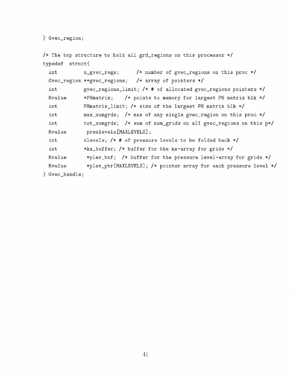
} Gvec_region;/* The top structure to hold all grd_regions on this processor */typedef struct{int n_gvec_regs; /* number of gvec_regions on this proc */Gvec_region **gvec_regions; /* array of pointers */int gvec_regions_limit; /* # of allocated gvec_regions pointers */Rvalue *PHmatrix; /* points to memory for largest PH matrix blk */int PHmatrix_limit; /* size of the largest PH matrix blk */int max_numgrds; /* max of any single gvec_region on this proc */int tot_numgrds; /* sum of num_grids on all gvec_regions on this p*/Rvalue preslevels[MAXLEVELS];int nlevels; /* # of pressure levels to be folded back */int *kx_buffer; /* buffer for the kx-array for grids */Rvalue *plev_buf; /* buffer for the pressure level-array for grids */Rvalue *plev_ptr[MAXLEVELS]; /* pointer array for each pressure level */} Gvec_handle;

41

Appendix C: GEOS 2.1 Data TypesC.1: Obs Vect Typetype Obs_Attinteger::kr,kt,kx,ks,kmreal::lat,lonend type Obs_Atttype Obs_Profinteger::nlevtype(Obs_Att)::attreal, pointer :: val(:)integer, pointer::qc(:)real, pointer::lev(:)end type Obs_Proftype Obs_Vectinteger::nproftype(Obs_Prof), pointer :: prof(:)end type Obs_VectC.2: State Vect Typetype State_Attinteger::kr,ktreal::lat,lonreal::x,yend type State_Atttype State_Profinteger::nlevtype(State_Att)::attreal, pointer :: val(:) 42

real, pointer::lev(:)real, pointer::z(:)end type State_Proftype State_Vectinteger::nproftype(State_Prof), pointer :: prof(:)end type State_VectC.3: Anal Vec Typetype Anal_Vectreal, pointer::us(:,:)real, pointer::vs(:,:)real, pointer::slp(:,:)real, pointer::u(:,:,:)real, pointer::v(:,:,:)real, pointer::h(:,:,:)real, pointer::q(:,:,:)end type Anal_Vect43

Appendix D: GEOS 3.0 Proposed Data TypesD.1: Gpt handle f90Note that Gpt holder f90 emulates the structure of Gpt handle that is used in PSASJPL.type Gpoint_f90real::coord(3)integer::orgn_procinteger::idend type Gpoint_f90type Gpt_region_f90integer::reg_idinteger::numGptsinteger::totlenreal::cent_mass(3)real::extension(3)integer::gpoints_limittype(Gpoint_f90),pointer::gpoints(:)end type Gpt_region_f90type Gpt_holder_f90integer::numRegstype(Gpt_region_f90),pointer::gpt_region(:)end type Gpt_holder_f9044

Appendix E: Notes on the JPL Parallel PSAS CodeE1. Where the JPL Parallel PSAS is ArchivedThe code is a public-domain code available through the High Performance Com-puting and Communications (HPCC) Software Exchange, and can be obtained viaanonymous ftp at the universal resource locator (URL)ftp://hera.gsfc.nasa.gov/pub/hpcc/PSAS.T3D.FIXED/mpiPSAS.tarNote that this tar �le contains both the source code and sample data, and thus isquite large. The total disk space needed for the tar �le alone is over 61 Mbytes, andthe directory tree structure that results when it is untarred occupies over 70 Mbytesof disk. To be safe, one should have on the order 150 Mbytes to download, compile,and run the JPL PSAS.E.2 About the Source Code for the Parallel PSASThe parallel PSAS is a hybrid code, comprising 105 �les of C source code (15107 linesof source code), along with 47 FORTRAN 77 �les (7623 lines of source code). Thesource code is organized in a directory hierarchy summarized below:� distr: This directory contains code that accomplishes the distribution of ma-trix blocks of the innovation matrix and related codes.� fill: Organize and �ll in blocks of the forecast error covariance matrix andrelated codes.� fold old: Solution of the innovation equation. This operation is sometimesreferred to as the foldback, since it involves folding the CG solution x from theobservation grid to the analysis grid.� ftrn new: FORTRAN codes containing the parameterizations of forecast errorcovariances, et cetera. One could argue that the bulk of the science behindPSAS lies here in these routines.� include: The header �les for all the C programs.� io: Input/Output-related codes, including read data.c, read parameter.c,et cetera.� misc: miscilaneous service routines, such as print matrix.c, printflag.c, etcetera. 45

� mv: The parallel matrix-vector multiplication code lies here, along with the restof the parallel conjugate-gradient solver (cg solver) source code.� part: Source code for both the parallel and sequential partitioners and theirrelated routines.� src: The driver program, main.c. As mentioned in the previous section, thisis the directory from which PSAS is compiled via the command make all� run: Directory from which one runs the parallel code. Sample input data,along with �le param.in, which contains the control parameters for the parallelPSAS. The �le Read.me contains detailed instructions on running the code,information regarding test cases, et cetera.E.3 Building the Executable JPL Parallel PSASOnce one has downloaded the tar �le mpiPSAS.tar, the procedure outlined belowshould be followed to build the executable. One should note that the current distri-bution of the code is con�gured to be compiled on either the Intel Paragon or theCray T3D (default).1. Create a directory as your main PSAS directory from which will serve as theroot, whose descendents will include directories containing all the source code,support data, and a directory from which to execute the code. The suggesteddirectory name is mpiPSAS (parallel PSAS). On Unix systems (and in thissection a unix-like operating system is assumed from this point foward), thisdirectory can be created by typing the command mkdir mpiPSAS2. Next, go to the mpiPSAS directory (use command cd mpiPSAS). Move the tar�le mpiPSAS.tar to this directory (or, for that matter, move to this directoryand download the tar �le mpiPSAS.tar into this directory). Unpack the tar�le using the command tar -xvf mpiPSAS.tar which will create the directorystructure containing the source code, data, et cetera.3. At this point, it is necessary to set some environment variables associated withthe compilation process using make, and also the execution of the code. In thedirectory mpiPSAS, typing the command source ./setupwill accomplish this.For the shells csh or tcsh, one can alter the .cshrc �le to set this variable byadding the line setenv PSASHOME mpiPSAS Adding this line to the .profile46

�le is necessary for users of the ksh and bash shells. In any event, this actionsets the environment variable PSASHOME, which can be veri�ed by the commandecho $PSASHOME4. Now it is possible to proceed with the installation of the code. In the directorympiPSAS/src type the command make all This is a lengthy process that ulti-mately produces the executable �le main, which is then moved to the directorympiPSAS/run.E.4 Running the JPL Parallel PSASOnce the code has been compiled, and is con�gured to run on nprocs processingelements, it may be run on the Cray T3D via the command main -npes nprocsIn order to run correctly, the contents of the parameter �le param.in have to bespeci�ed correctly. Below is a listing of the parameters found in param.in, along withtheir signi�cance. A sample listing of param.in can be found in Appendix E.5. Notethat the entries in the parameter �le must be in order and with no omissions.� datafile= the input data �le containing innovations.� incvfile= the output data �le, containing the analysis increment vectors� nobs= the number of observations� totregns= the total number of observation regions� max iter= the maximumnumber of iterations for the Conjugate Gradient (CG)solver� precond iter= maximum number of iterations for the preconditioner to theCG solver� tolerance= fractional change at which CG solver terminates successfully� precond tol= same as above for the preconditioner CG solver� decimate= 1 for equal-area grids, 0 otherwise� write incvc= 0=no write; 1= to binary �le incvec.out; 2=to stdout� want slu= 1 fold back sea level u-wind, 0 otherwise47

� want slv= 1 fold back sea level v-wind, 0 otherwise� want slp= 1 fold back sea level pressure, 0 otherwise� want uwnd= 1 fold back up air u-wind, 0 otherwise� want vwnd= 1 fold back up air v-wind, 0 otherwise� want hght= 1 fold back up air geo hight, 0 otherwise� want mixr= 1 fold back up air mix ratio, 0 otherwise� plevel low= Upper air pressure level lower limit� plevel high= Upper air pressure level upper limit� ncols= Number of columns of processors� nrows= Number of rows of processors� printflag= Printging ags. set print ag=-1 will give all options� ebugflag= Debugging ags. set print ag=-2 will give all options� printproc= The processor on which data are printed.� stopflag= > 0 stop execution at the ith place. � 0 no stop� freeflag= Free parameter for convenience. Can be used for anything� rho= Parameter used in simulated annealing load-balance algorithm for maxtrixblock distribution (currently not used)� beta= Parameter used in simulated annealing load-balance algorithm for max-trix block distribution (currently not used)� rm seed= Random number seed for maxtrix block distribution load balancingscheme� niter= Number of iterations for maxtrix block distribution load balancingscheme. 48

E.5 Procedures for Modifying the Source CodeThe make�le system for the source code is a multi-directory, two-pass system with allthe necessary cross-checking of dependencies. All relations are speci�ed in one andonly in one place. A modi�cation of the makefile (e.g., adding a source code �le)should be made in makefile.org, not makefile. The dependencies on the header�les will be accounted for automatically. After a change of makefile.org in one orany directories, all you need to do to re-compile the codes is to type make all in thempiPSAS/src directory.If one wishes to modify any of the C or FORTRAN source code, or modify any ofthe header (.h) �les, one can, following this procedure:1. Go to the relevant directory, and edit the C (.c), FORTRAN (.f), or header(.h) �le2. In that directory, type the command make all3. Go to the mpiPSAS/src directory, and type the command make all to build anew executable main. Note that one can skip step 2 and simply execute thisstep with the same result.If one wishes to modify the source code by adding further source code �les (C orFORTRAN), it is accomplished as follows:1. Go the relevant directory and add the new source code �le2. Change the makefile.org �le to re ect this new source code3. Type the command make makefile in that directory, which will create a newmakefile.4. Type command make all in that directory.5. Go to the directory mpiPSAS/src and type the command make all to get a newexecutable main. Note that this step alone can accomplish what was outlinedin the two previous steps.If one wishes to refresh �le dependecies, change or split header �les into moreheader �les, et cetera, such actions are equivelent to rebuilding the entire PSASsystem. Here is what needs to be done subsequent to such changes:49

1. Execute the command touch makefile.org in the appropriate or all direc-tories. This can also be done via touch */makefile.org from the directorympiPSAS/src.2. Go to the directory mpiPSAS/src and type the command make all to build thenew executable main.Finally, it should be noted that there are �les present in the source code direc-tory hierarchy that are needed by make to correctly implement the cross-directorycompilation procedure. If these �les are missing or incorrectly modi�ed, make couldfail.� The �le mpiPSAS/compile contains prede�ned ags and variables used by make.� In each of the source code subdirectories, there should be a makefile, whichcontains make rules for the �les in that directory� In each of the source code subdirectories, there is a �le entitled LINKFILES, inwhich �lename and dependency information to the master make�le in mpiPSAS/src.It is generated from the local makefile.

50

E.6 Sample Input Parameter File param.indatafile=dataCRAY.51990 /* input data file */incvfile=incvec.51990 /* output data file, increment vectors */nobs=51990 /* number of observations */totregns=512 /* number of observation regions */max_iter=150 /* max iteration in Preconditioned Conjugate Gradt solver */precond_iter=150 /* max iter in the Preconditioner which is also a CG solver */tolerance=0.001 /* residual reduction factor in PCG solver */precond_tol=0.001 /* residual reduction in the Preconditioner itself */decimate=1 /* 1 for equal-area grids, 0 otherwise */write_incvc=1 /* 0=no write; 1= to binary file incvec.out; 2=to stdout */want_slu=0 /* 1 fold back sea level u-wind, 0 otherwise */want_slv=0 /* 1 fold back sea level v-wind, 0 otherwise */want_slp=0 /* 1 fold back sea level pressure, 0 otherwise */want_uwnd=1 /* 1 fold back up air u-wind, 0 otherwise */want_vwnd=1 /* 1 fold back up air v-wind, 0 otherwise */want_hght=1 /* 1 fold back up air geo hight, 0 otherwise */want_mixr=1 /* 1 fold back up air mix ratio, 0 otherwise */plevel_low=19.0 /* pressure level lower limit : min=9.0 */plevel_high=1501.0 /* pressure level upper limit : max=1001.0 */ncols=0 /* the # of processors on columes */nrows=1 /* the # of processors on rows */printflag=0 /* printging flags. set printflag=-1 will give all options */debugflag=0 /* debugging flags. set printflag=-2 will give all options */printproc=0 /* the processor on which data are printed. */stopflag= 0 /* >0 stop execution at the ith place. <=0 no stop. */freeflag=-19 /* Free parameter for convenience. Can be used for anything */rho=1.0 /* for maxtrix block distribution */beta=10. /* for maxtrix block distribution */rm_seed=12345 /* for maxtrix block distribution */niter=10 /* for maxtrix block distribution *//* Don't change the sequential order of lines. They are important */51

Appendix F: Workshop ParticipantsWorkshop I: September 30 - October 4, 1996, DAO, Goddard Space Flight Center(GSFC), Greenbelt, Maryland.� P. M. Lyster (chair), Meteorology Department and Joint Center for Earth Sys-tem Science (JCESS), University of Maryland.� A. M. daSilva, General Sciences Corporation and NASA Goddard Space FlightCenter (GSFC)� C. H. Q. Ding, Lawrence Berkeley National Laboratory� Jing Guo, General Sciences Corporation� J.W. Larson, Department of Earth and Atmospheric Sciences, Purdue University2� I. �Stajner, Universities Space Research AssociationWorkshop II: October 28 - November 1, 1996, DAO GSFC.� P. M. Lyster (chair), Meteorology Department and Joint Center for Earth Sys-tem Science, University of Maryland.� A. M. daSilva, General Sciences Corporation and NASA Goddard Space FlightCenter (GSFC)� Jing Guo, General Sciences Corporation� J. W. Larson, JCESS, University of Maryland� W. Sawyer, ELCA Informatique3� I. �Stajner, Universities Space Research Association2Current A�liation: Dept. of Meteorology and JCESS, University of Maryland3Current A�liation: Dept. of Meteorology and JCESS, University of Maryland52

Appendix G: Figures

w - H w

innovations

observations

forecast

PSAS

fo

initialization

analysis

COUPLER

OBS / QCGCM

Figure 1: PSAS and its role in GEOS-DAS.53

Mblk_list* ,MPI_Comm*

Reg_replica_handle* , Mblk_list* , MPI_Comm* )

partitioner( Obs_handle* , MPI_Comm* )

matrix_distr( Obs_handle* , Vec_handle* ,

COMPUTATION

allocate_obs_handle(2*totregions/activeProcs)

allocate_vec_handle(globals.totregns + 1)

exit()

main()INITIALIZATION

equation_solve( Vec_handle* , Reg _replica_handle* ,

MPI_Comm* )

read_param("param.in", MPI_Comm* )

printflag_table(globals.printflag)

print_functions()

read_data( char *datfile, int nobs, Obs_handle*,

foldback( Vec_handle* , MPI_Comm* )

)

MPI_Comm_dup( MPI_COMM_WORLD, MPI_Comm* )

MPI_Init(&argc, &argv)

init_glob_comm_env( MPI_Comm* )

Figure 2: Top-level owchart of parallel PSAS.

54

ObservationsPartition’boundary’Figure 3: Parallel partition of observations into regions using recursive bisection.

55

##############################

#########################

##############################

#########################

##############################

##############################

##############################

Figure 4: Matrix-block distribution of the innovation matrixHP fHT +R The upper-half blocks of the complete symmetric matrix are assembled on each processor.56

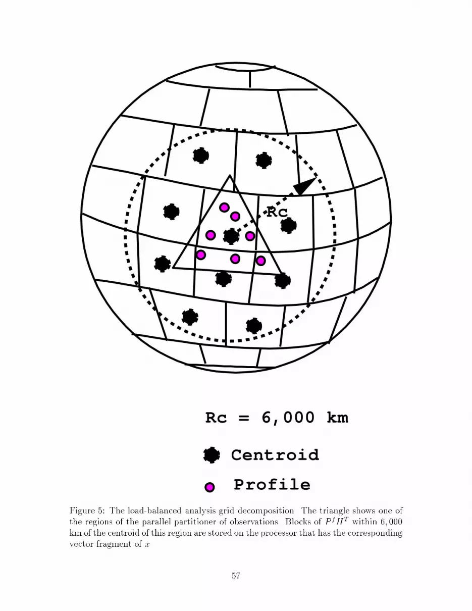
Rc = 6,000 km

Rc

Centroid

ProfileFigure 5: The load-balanced analysis grid decomposition. The triangle shows one ofthe regions of the parallel partitioner of observations. Blocks of P fHT within 6; 000km of the centroid of this region are stored on the processor that has the correspondingvector fragment of x 57

0 128 256 384 512Number of Processors

0.0

1.0

2.0

3.0

4.0

5.0

6.0

7.0

8.0

9.0

10.0

11.0

12.0

Perf

orm

ance

(Gig

aflo

ps)

Prototype Parallel PSASPerformance on 512 Node Cray T3D

51,990 Observations79,938 Observations

Figure 6: Performance (giga op/s) of the PSAS JPL on the Goddard 512 processorCray T3D using the MPI message-passing library. The closed circles are for a problemwith 51; 990 observations and the open circles are for 79; 938 observations.58

Schematic representation of a block of Chh

Figure 7: Every I � I block Chh(j; k; '1; '2) is a circulant symmetric matrix. Theelements along its lth and (I� l)th superdiagonals and subdiagonals are identical forevery l, 0 � l � I � 1. 59