Embed Size (px)
Citation preview
DESIGN OPTIMIZATION OF COMPOSITE DEPLOYABLE BRIDGE
SYSTEMS USING HYBRID META-HEURISTIC METHODS FOR
RAPID POST-DISASTER MOBILITY
ASHRAF MOHAMED AHMED OSMAN
A Thesis
In the Department
of
Building, Civil and Environmental Engineering
Presented in Partial Fulfillment of the Requirements
For the Degree of
Doctor of Philosophy (Civil Engineering) at
Concordia University
Montréal, Québec, Canada
August 2016
© ASHRAF OSMAN, 2016

iii
Concordia University
School of Graduate Studies
This is to certify that the thesis prepared
By: Mr. Ashraf Mohamed Ahmed Osman
Entitled: Design Optimization of Composite Deployable Bridge Systems Using Hybrid
Meta-Heuristic Methods for Rapid Post-disaster Mobility
and submitted in partial fulfillment of the requirements for the degree of
Doctor of Philosophy (Building, Civil and Environmental Engineering)
Complies with the regulations of this University and meets the accepted standards with respect to originality and quality.
Signed by the final examining committee:
Chair Dr. A. Awasthi External Examiner Dr. Ex Maged A. Youssef Examiner, External to Program Dr. R. Sedaghati Examiner Dr. A. Bagchi Examiner Dr. A. Bhowmick Supervisor Dr. K. Galal
Approved by:
Fariborz Haghighat, Ph.D., P.Eng, Graduate Program Director
Department of Building, Civil and Environmental Engineering
August 22, 2016
Dr. Amir Asif, Ph.D., PEng, Dean
Faculty of Engineering and Computer Science
iii
ABSTRACT
Design optimization of composite deployable bridge systems using hybrid
meta-heuristic methods for rapid post-disaster mobility
Ashraf Mohamed Ahmed Osman, Ph.D.
Concordia University, 2016
Recent decades have witnessed an increase in the transportation infrastructure damage caused
by natural disasters such as earthquakes, high winds, floods, as well as man-made disasters. Such
damages result in a disruption to the transportation infrastructure network; hence, limit the post-
disaster relief operations. This led to the exigency of developing and using effective deployable
bridge systems for rapid post-disaster mobility while minimizing the weight to capacity ratio.
Recent researches for assessments of mobile bridging requirements concluded that current
deployable metallic bridge systems are prone to their service life, unable to meet the increase in
vehicle design loads, and any trials for the structures’ strengthening will sacrifice the ease of
mobility. Therefore, this research focuses on developing a lightweight deployable bridge system
using composite laminates for lightweight bridging in the aftermath of natural disaster. The
research investigates the structural design optimization for composite laminate deployable bridge
systems, as well as the design, development and testing of composite sandwich core sections that
act as the compression bearing element in a deployable bridge treadway structure.
The thesis is organized into two parts. The first part includes a new improved particle swarm
meta-heuristic approach capable of effectively optimizing deployable bridge systems. The
developed approach is extended to modify the technique for discrete design of composite laminates
and maximum strength design of composite sandwich core sections. The second part focuses on
developing, experimentally testing and numerically investigating the performance of different
sandwich core configurations that will be used as the compression bearing element in a deployable
fibre-reinforced polymer (FRP) bridge girder.
iv
The first part investigated different optimization algorithms used for structural optimization.
The uncertainty in the effectiveness of the available methods to handle complex structural models
emphasized the need to develop an enhanced version of Particle Swarm Optimizer (PSO) without
performing multiple operations using different techniques. The new technique implements a better
emulation for the attraction and repulsion behavior of the swarm. The new algorithm is called
Controlled Diversity Particle Swarm Optimizer (CD-PSO). The algorithm improved the
performance of the classical PSO in terms of solution stability, quality, convergence rate and
computational time. The CD-PSO is then hybridized with the Response Surface Methodology
(RSM) to redirect the swarm search for probing feasible solutions in hyperspace using only the
design parameters of strong influence on the objective function. This is triggered when the
algorithm fails to obtain good solutions using CD-PSO. The performance of CD-PSO is tested on
benchmark structures and compared to others in the literature. Consequently, both techniques, CD-
, and hybrid CD-PSO are examined for the minimum weight design of large-scale deployable
bridge structure. Furthermore, a discrete version of the algorithm is created to handle the discrete
nature of the composite laminate sandwich core design.
The second part focuses on achieving an effective composite deployable bridge system, this is
realized through maximizing shear strength, compression strength, and stiffness designs of light-
weight composite sandwich cores of the treadway bridge’s compression deck. Different composite
sandwich cores are investigated and their progressive failure is numerically evaluated. The
performance of the sandwich cores is experimentally tested in terms of flatwise compressive
strength, edgewise compressive strength and shear strength capacities. Further, the cores’
compression strength and shear strength capacities are numerically simulated and the results are
validated with the experimental work. Based on the numerical and experimental tests findings, the
sandwich cores plate properties are quantified for future implementation in optimized scaled
deployable bridge treadway.
KEYWORDS: Meta-heuristic algorithm, Swarm intelligence, Particle swarm optimizer, Controlled
diversity, composite sandwich cores, deployable bridges, CFRP beams.

v
To my beloved parents

vi
ACKNOWLEDGEMENT
The author would like to express his sincere appreciation and gratitude to his supervisor and
mentor for his guidance and technical support.
Also, he would like to acknowledge the assistance of Mr. Daniel Stubbs during the numerical
work over Quebec clusters, as well the promising engineer and the NSERC student Mr. Navid
Assemani for his help and assistance in the numerical simulation which is highly appreciated. In
addition, he would like to express his gratitude to Dr. Omar Yakob, Mr. Yasser Elsherbiny, and
Mr. Hassan Alshahrani for their great support in the experimental work.
He would like to thank his parents, for their endless love, support, and encouragement through
his entire life. They are the main contributors and perform the instrumental role in his life`s
development in terms of personality and education. He owes them a debt of gratitude.
Finally, he would like to thank his wife Shaimaa for her patience, endless spiritual support and
loving concern. He is forever indebted to her for bearing his long hours of work and busy schedule.
He would dedicate the favor of any achievement he could make in this work for her invaluable
supporting during his study. Last but not least, he would like to express his deep adoration and
love for his little kids, Karma and Omar.
vii
TABLE OF CONTENTS
INTRODUCTION ..................................................................................... 1
1.1 PROBLEM STATEMENT ........................................................................................ 1
1.2 RESEARCH SIGNIFICANCE AND MOTIVATION ...................................................... 2
1.3 OBJECTIVES AND SCOPE OF WORK ...................................................................... 7
1.4 THESIS LAYOUT ................................................................................................10
CHAPTER 2 LITERATURE REVIEW ..........................................................................11
2.1 INTRODUCTION..................................................................................................11
2.2 MILITARY BRIDGE SOLUTIONS..........................................................................11
2.2.1 ASSAULT BRIDGE SYSTEMS ........................................................................................ 12
I. CLOSE SUPPORT BRIDGE (BR-90)........................................................................ 12
II. WOLVERINE HEAVY ASSAULT BRIDGE (HAB) .................................................... 13
2.2.2 TACTICAL BRIDGE SOLUTIONS ................................................................................... 14
I. MEDIUM GIRDER BRIDGE (MGB) ........................................................................ 14
II. DRY SUPPORT BRIDGE (DSB) .............................................................................. 15
viii
2.3 DEPLOYABLE COMPOSITE BRIDGES ..................................................................16
2.4 OTHER RESEARCH EFFORTS FOR POST DISASTER MOBILITY ............................19
2.5 SUMMARY .........................................................................................................24
CHAPTER 3 STRUCTURAL DESIGN OPTIMIZATION AND SOLUTION TECHNIQUES ......26
3.1 INTRODUCTION..................................................................................................26
3.2 OPTIMIZATION TECHNIQUES .............................................................................26
3.2.1 ASSESSMENT OF OPTIMIZATION SOLUTIONS ............................................................... 27
3.2.1.1 GENETIC ALGORITHMS ................................................................................. 28
3.2.1.2 OPTIMIZATION METHODS BUILT IN FE PACKAGE (ANSYS) ........................ 30
3.2.2 ASSESSMENT PROCEDURE ........................................................................................... 31
3.2.3 THE DEPLOYABLE BRIDGE SYSTEM ............................................................................ 32
3.2.3.1 NUMERICAL SIMULATION ............................................................................. 34
3.2.3.2 NUMERICAL EVALUATION ............................................................................ 34
3.3 SUMMARY .........................................................................................................39
CHAPTER 4 CONTROLLED-DIVERSITY SWRAM OPTIMIZATION .............................40
4.1 INTRODUCTION..................................................................................................40
4.2 PARTICLE SWARM OPTIMIZATION ALGORITHM .................................................40
4.3 BACKGROUND OF STRUCTURAL OPTIMIZATION USING PSO .............................42
4.4 CONTROLLED DIVERSITY ..................................................................................44
4.4.1 CONTROLLING ATTRACTION AND REPULSION OF THE SWARM ..................................... 44
ix
4.4.2 LEVY FLIGHT PSO FOR STRUCTURAL OPTIMIZATION................................................... 47
4.5 ASSESSMENT OF CD-PSO ON BENCHMARK STRUCTURES.................................48
4.5.1 PROBLEMS FORMULATION AND FEASIBILITY MANAGEMENT ...................................... 48
4.5.2 10-MEMBER PLANAR TRUSS ........................................................................................ 50
I. CD-PSO CONCEPT EVALUATION .......................................................................... 51
II. COMPARISONS WITH OTHER OPTIMIZATION ALGORITHMS .................................... 53
4.5.3 25-MEMBER SPATIAL TRUSS ........................................................................................ 54
4.5.4 72-MEMBER SPATIAL TRUSS ........................................................................................ 57
4.6 ASSESSMENT OF HYBRID AND ORIGINAL CD-PSO ...........................................60
4.6.1 RESPONSE SURFACE METHODOLOGY (RSM) .............................................................. 61
4.6.2 HYBRID CD-PSO ........................................................................................................ 63
4.6.3 NUMERICAL RESULTS .................................................................................................. 69
4.7 CONCLUSIONS ...................................................................................................73
4.7.1 CD-PSO APPLICATION ON BENCHMARK STRUCTURES ................................................ 73
4.7.2 HYBRID AND ORIGINAL CD-PSO APPLICATION ON DEPLOYABLE BRIDGE STRUCTURE 74
4.8 SUMMARY .........................................................................................................75
CHAPTER 5 DEVELOPMENT AND TESTING OF NEW COMPOSITE DECKS .................76
5.1 INTRODUCTION..................................................................................................76
5.2 COMPOSITE PROCESSING METHODS ..................................................................77
5.2.1 WET LAYUP ................................................................................................................ 77
5.2.2 RESIN TRANSFER MOLDING (RTM) ............................................................................ 78
5.2.3 VACUUM ASSISTED RESIN TRANSFER MOLDING (VARTM) ...................................... 79
x
5.2.4 FILM RESIN INFUSION MOLDING (FRIM) .................................................................... 80
5.2.5 OUT OF AUTOCLAVE AND AUTOCLAVE PROCESS ........................................................ 81
5.2.6 FILAMENT WINDING PROCESS .................................................................................... 81
5.2.7 PULTRUSION PROCESS ................................................................................................ 82
5.2.8 COMPARISON OF MANUFACTURING PROCESSES ......................................................... 83
5.3 EFFECTIVE COMPOSITE BRIDGING ....................................................................84
5.3.1 DECK DEVELOPMENT .................................................................................................. 85
5.3.2 CORES DESCRIPTION AND MANUFACTURING .............................................................. 85
• CORE 1: (A1-HC-W) ........................................................................................... 87
• CORE 2: (A2-HC-CP) .......................................................................................... 88
5.3.3 DESIGN AND BUCKLING ANALYSIS ............................................................................. 94
5.4 EXPERIMENTAL TEST SETUPS ...........................................................................95
5.4.1 MATERIAL CHARACTERIZATION ................................................................................. 95
5.4.2 SHEAR USING THREE POINTS LOADING TEST .............................................................. 98
5.4.3 FLATWISE COMPRESSION TEST ................................................................................. 100
5.5 TEST RESULTS AND DISCUSSIONS ...................................................................102
5.5.1 SHEAR USING THREE POINTS LOADING TEST ............................................................ 102
5.5.2 FLATWISE COMPRESSION TEST ................................................................................. 105
5.5.3 COMPARISON WITH CFRP WEBBED CORES .............................................................. 107
5.6 NUMERICAL SIMULATION ...............................................................................109
5.6.1 FINITE ELEMENT MODELING ..................................................................................... 109
5.6.2 PROGRESSIVE DAMAGE MODELING .......................................................................... 110
5.6.3 MATERIAL DEGRADATION RULES ............................................................................. 113
xi
5.6.4 SHEAR TEST SIMULATION ......................................................................................... 114
5.6.5 COMPRESSION TEST SIMULATION ............................................................................. 118
5.7 SUMMARY AND DESIGN RECOMMENDATIONS .................................................121
5.8 CONCLUSIONS AND PERFORMANCE CRITERIA .................................................125
CHAPTER 6 STRENGTH OPTIMIZATION OF COMPOSITE DEPLOYABLE BRIDGE DECKS
................................................................................................................................126
6.1 INTRODUCTION................................................................................................126
6.2 DESIGN APPROACH .........................................................................................127
6.2.1 LOADS ANALYSIS...................................................................................................... 128
6.2.2 LAMINATE ANALYSIS ................................................................................................ 133
6.2.3 FAILURE ANALYSIS ................................................................................................... 135
6.3 DISCRETE CD-PSO FOR LAMINATED STRUCTURES ........................................137
6.3.1 DISCRETE FORMULATION OF CD-PSO ...................................................................... 138
6.3.2 HEURISTIC CONTROLLED DIVERSITY PARTICLE SWARM HCD-PSO ........................ 139
6.3.3 FLY-BACK MECHANISM FOR HCD-PSO ................................................................... 140
6.4 ASSESSMENT OF HCD-PSO ............................................................................141
6.5 HCD-PSO APPLICATION ON COMPOSITE CORE DECKS ..................................144
6.6 SUMMARY AND CONCLUSIONS ........................................................................146
CHAPTER 7 ..........................................................................................................148
7.1 OPTIMIZATION OF DEPLOYABLE BRIDGES .......................................................148
xii
7.2 COMPOSITE DEPLOYABLE BRIDGE DECKS ......................................................149
7.3 STRENGTH DESIGN OPTIMIZATION OF COMPOSITE CORES ..............................150
7.3 CONTRIBUTIONS ..............................................................................................151
7.3 LIMITATIONS ...................................................................................................152
7.4 FUTURE WORK ................................................................................................153
........................................................................................................155
........................................................................................................156
........................................................................................................157
xiii
LIST OF FIGURES
Figure 1.1. Bohol, Philippines Earthquake, Oct 2013, (Web-1) ..................................................... 1
Figure 1.2. New Jersey, N.Y., USA, Hurricane Sandy, Oct 2013, (Web-2) .................................. 1
Figure 1.3. Ibo River (Japan) flood by Typhoon, Aug 2009, (Web-3) ........................................... 1
Figure 1.4. Crossing spans percentage of natural gaps’ in different territories .............................. 3
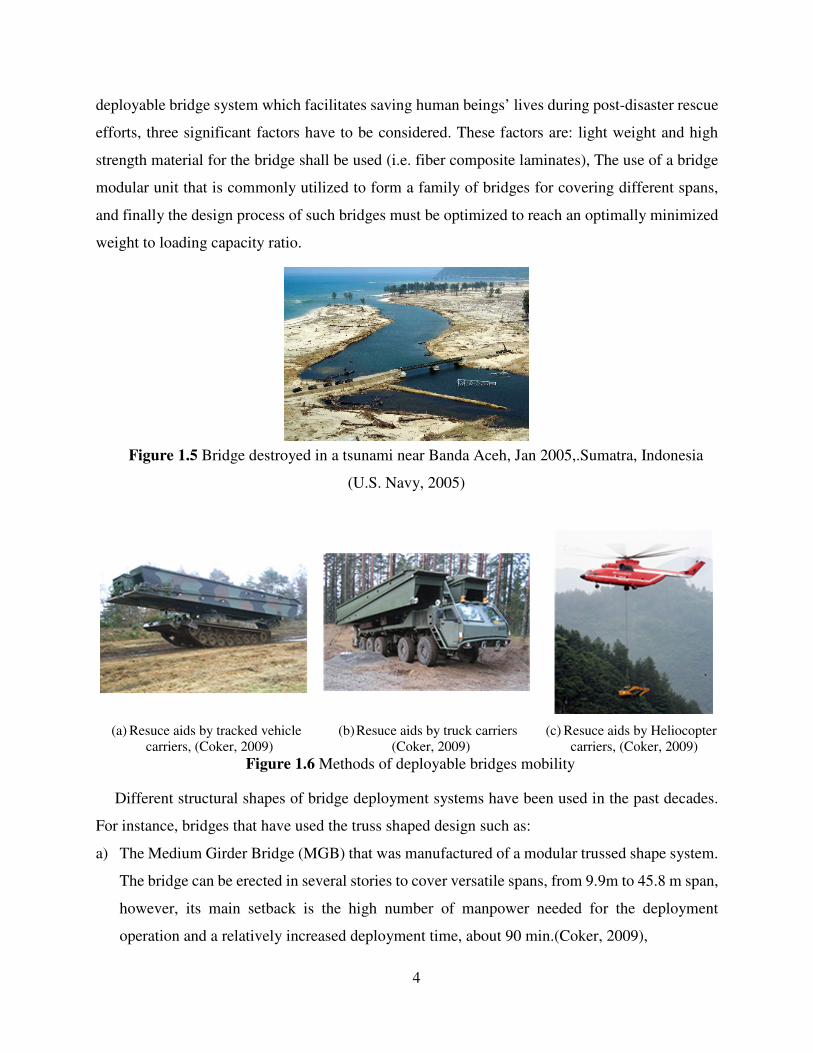
Figure 1.5. Bridge destroyed in a tsunami near Banda Aceh, Jan 2005,.Sumatra, Indonesia (U.S.
Navy, 2005)..................................................................................................................................... 4
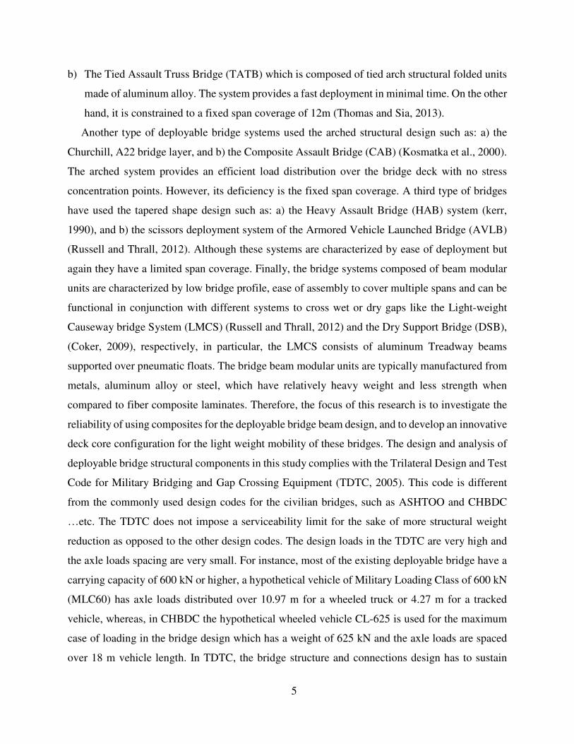
Figure 1.6. Methods of deployable bridges mobility ...................................................................... 4
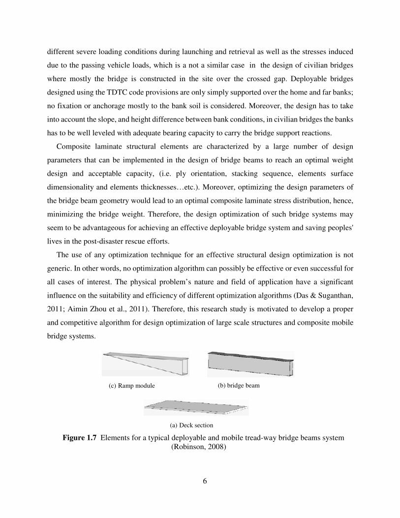
Figure 1.7. Elements for a typical deployable and mobile tread-way bridge beams system
(Robinson, 2008)............................................................................................................................. 6
Figure 2.1. Deployed Axially Tensioned Long Span Bridge (ATLSB/BR-90) (Winney, 1994) . 12
Figure 2.2. Close Support Bridge No.10 being launched (Winney, 1994) ................................... 13
Figure 2.3. Wolverine Heavy Assault Bridge being launched (Coker, 2009) .............................. 13
Figure 2.4. MGB single storey bridge with aluminum girders (9.9m span), (Web-4) ................. 14
Figure 2.5. MGB double storey bridge with truss girder reinforcement (31m span) , (Web-4) ... 14
Figure 2.6. MGB Three storey bridge with link reinforcement to the truss girder (45.8m span) ,
(Web-4) ......................................................................................................................................... 15
Figure 2.7. Launching and retrieval mechanism of the DSB Bridge system, (Web-5) ................ 16
Figure 2.8. The DSB being launched across a gap, (Web-5) ........................................................ 16
Figure 2.9. An Isometry of the Composite Army Bridge (CAB) system, (Kosmatka, 2011) ...... 17
Figure 2.10. An exploded view illustrating the Composite Army Bridge (CAB) components
(Kosmatka et al., 2000) ................................................................................................................. 17
Figure 2.11. Schematic for SCRIMP technique, (Robinson and Kosmatka, 2008) ...................... 18
Figure 2.12. M113 during a dynamic test for the short span composite bridge, .......................... 18
Figure 2.13. The GFRP bridge beam during a crossing test by Bison armored vehicle (9.2 m span),
(Landherr, 2008) ........................................................................................................................... 19
Figure 2.14. Cross section, launching and retrieval Concepts of the 15 m deployable bridge
(Lederman et al., 2014) ................................................................................................................. 20
Figure 2.15. Concept of the construction sequence for the deployable bridge using the composite
SIP forms (Hanus et al., 2008)..................................................................................................... 21
xiv
Figure 2.16. Discretization of a continuum body into micro truss elements (Ario et al., 2013) .. 22
Figure 2.17. Photograph of the experimental testing of the scissors bridge after been deployed
(Ario et al., 2011).......................................................................................................................... 22
Figure 2.18. Hybrid FRP-aluminum space truss bridge design concept: ..................................... 23
Figure 2.19. Configuration of trussed members (dimensions in mm) (Zhang et al., 2014) ......... 24
Figure 2.20. Configuration of the bridge and cross section of I beams (Zhang et al., 2014) ....... 24
Figure 3.1. Publications distribution for applying meta-heuristic optimization in engineering
problems ........................................................................................................................................ 27
Figure 3.2. Sexual recombination to generate an offspring through crossover and mutation ...... 29
Figure 3.3. Flowchart of the structural design optimization procedure ........................................ 31
Figure 3.4. An exploded view of the 24 m bridge assembly (Osman, 2006) ............................... 32
Figure 3.5. Tread-way beams cross-section .................................................................................. 33
Figure 3.6. Convergence history comparison of the applied methods .......................................... 37
Figure 3.7. Representation of the principal streses distribution over the bridge structure at the
critical loading case....................................................................................................................... 38
Figure 4.1. Particle updating velocity scheme .............................................................................. 42
Figure 4.2. The trajectory variation of the classical PSO, ARPSO, and CD-PSO Diversity. ...... 47
Figure 4.3. A 10-member planar truss .......................................................................................... 51
Figure 4.4. The optimized material distribution of 10-member truss. .......................................... 52
Figure 4.5. Convergence history of CD-PSO compared to other PSO algorithms. ...................... 53
Figure 4.6. A 25-member spatial truss. ......................................................................................... 55
Figure 4.7. Convergence history of CD-PSO and classical PSO best for the 25-member spatial
truss. .............................................................................................................................................. 56
Figure 4.8. A 72-member spatial truss. ......................................................................................... 58
Figure 4.9. Convergence history of CD-PSO and classical PSO best for the 72-member spatial
truss. .............................................................................................................................................. 60
Figure 4.10. Schematic illustration of using DOE and RSA for multi-step design optimization 63
Figure 4.11. Flowchart illustration of hybrid CD-PSO with RSM ............................................... 68
Figure 4.12. Convergence history for the 24 m (78.74 ft) deployable bridge structure. .............. 73
Figure 5.1. Schematic of the Wet Layup Method ......................................................................... 77
Figure 5.2. Schematic of the Resin Transfer Molding Process (RTM) ........................................ 79
xv
Figure 5.3. Schematic of Seaman Composite Resin Infusion Molding Process (SCRIMP), ....... 80
Figure 5.4. Schematic of the Resin Film Infusion Molding Process (FRIM) ............................... 80
Figure 5.5. Schematic of the Out of Autoclave Process (OOA) ................................................... 81
Figure 5.6. Schematic of the Filament Winding Process (Hoa, 2009) ......................................... 82
Figure 5.7. Schematic of the Pultrusion process ........................................................................... 83
Figure 5.8. Balsa core applied for CAB deployable bridge .......................................................... 86
Figure 5.9. CFRP webbed core with foam infill (C4-TC) ............................................................ 87
Figure 5.10. CFRP webbed core with trapezoidal shape (C5-CC) ............................................... 87
Figure 5.11. An illustration of core A1-HC-W design configuration ........................................... 89
Figure 5.12. An illustration of core A2-HC-CP design configuration .......................................... 89
Figure 5.13. A photograph of the A1-HC-W fabricated core specimen ....................................... 89
Figure 5.14. A photograph of the A2-HC-CP fabricated core specimen ...................................... 90
Figure 5.15. A photograph of the A1-HC-W being post cured in Autoclave ............................... 91
Figure 5.16. A schematic of the infusion strategy used for the core specimens ........................... 91
Figure 5.17. A photograph of the A2-HC-CP specimen being infused with resin ....................... 92
Figure 5.18. A photograph of an analyzed microscopic sample ................................................... 92
Figure 5.19 Schematic of the possible local buckling modes of the sandwich cores ................... 94
Figure 5.20 An illustration of the out of plane acting loads and the generated load response by the
foam and web stiffness.................................................................................................................. 95
Figure 5.21. Photographs of testing the coupon samples over different machines ....................... 96
Figure 5.22. A photograph of a core beam during a three point load test .................................... 99
Figure 5.23. Illustration of the three point binding displacement potentiometers and strain gauges
locations ...................................................................................................................................... 100
Figure 5.24 Flatwise compression test setup of the reproduced C4-TC core ............................. 101
Figure 5.25 Photograph of the shear failure mode of core A1-HC-W during three points loading
test ............................................................................................................................................... 103
Figure 5.26 Photograph of the shear failure mode of core A2-HC-CP during three points loading
test ............................................................................................................................................... 103
Figure 5.27 Illustration of intelaminar shear failure modes of cores A1-HC-W and A2-HC-CP
..................................................................................................................................................... 104
Figure 5.28 Stress-Strain relation-ship of core A1-HC-W in the mid-span location .................. 105
xvi
Figure 5.29 Photograph illustrating the in-plane shear failure of cores during the compression test
..................................................................................................................................................... 106
Figure 5.30 Finite element mapped meshing of A1-HC-W core ................................................ 110
Figure 5.31 Flowchart illustrating the progressive failure model ............................................... 111
Figure 5.32 On-axis stress components on a layered composite element................................... 113
Figure 5.33 Illustration of the progressive damage predicted by the model in a three points loading
simulation at different load steps ................................................................................................ 115
Figure 5.34 Pictures showing failure validation under delamination in tension and compression of
both cores A1-HC-W and A2-HC-CP ........................................................................................ 116
Figure 5.35 Partial separation of the upper skin and core cross-section due to delamination failure
just near the machine loading foot print ..................................................................................... 117
Figure 5.36 Plot charts of the number of failed elements counts at each failure criterion ........ 119
Figure 5.37 Illustration of A1-HC-W degraded model in a compression test at different load steps
..................................................................................................................................................... 119
Figure 5.38 Pictures showing delamination failure in tension and compression of both cores A1-
HC-W and A2-HC-CP in the flatwise compression test ............................................................. 120
Figure 5.39 Plot of shear and compressive strength performance of different sandwich cores . 123
Figure 5.40 Plot of shear and compressive strength to core areal weight ratio normalized to balsa
system ......................................................................................................................................... 124
Figure 5.41 Plot of experimental and numerical strength performance to core areal weight ratios
..................................................................................................................................................... 124
Figure 6.1 Design approach definition (Kosmatka et al., 2000) ................................................. 128
Figure 6.2 Shear envelope of MLC70 and MLC100 design loads on a 12.7 m bridge design span
..................................................................................................................................................... 130
Figure 6.3 Moment envelope of MLC70 and MLC100 design loads on a 12.7 m bridge design span
..................................................................................................................................................... 130
Figure 6.4 Shear envelope of MLC30 and MLC50 design loads on a 12.7 m bridge design span
..................................................................................................................................................... 131
Figure 6.5 Moment envelope of MLC30 and MLC50 design loads on a 12.7 m bridge design span
..................................................................................................................................................... 131
xvii
Figure 6.6 Illustration of a thin composite laminate plate subjected to forces and moments
resultants ..................................................................................................................................... 132
Figure 6.7 Illustration of an enlarged view of a laminate cross-section ..................................... 133
Figure 6.8 Illustration of Tsai-Wu quadratic failure envelope ................................................... 137
Figure 6.9 Illustration of the possibilities of a particles’ violation to the problem feasibility
constraint or the variables’ boundary constraint ......................................................................... 138
Figure 6.10 Illustration of the fly-back mechanism .................................................................... 141
Figure 6.11 Convergence history of the strength ratio for the different PSO versions under the
application of bi-axial loading condition. ................................................................................... 142
Figure 6.12 Convergence history of the strength ratio for the different PSO versions under the
application of bi-axial and shear loading conditions .................................................................. 143
Figure 6.13 Convergence history of the strength ratio for cores A1-HC-W and A2-HC-CP for
different loadings ........................................................................................................................ 146
Figure C.1 A photograph of assembling the wrapped honeycomb beams and the triangular foam
filler of core A1-HC-W ............................................................................................................... 157
Figure C.2 A photograph of the polyisocyanurate foam beams assembly of core A2-HC-CP .. 157
Figure C.3 A photograph of the wrapped honeycomb beams, trapezoidal beams, and the corrugated
preform assembly of core A2-HC-CP ......................................................................................... 158
Figure C.4 A photograph of the sandwich construction in between the skins of core A2-HC-CP
..................................................................................................................................................... 158
Figure C.5 Compressive Stress-Strain curves of coupons at [05]T ............................................. 159
Figure C.6 Compressive Stress-Strain curves of coupons at [905]T ........................................... 159
Figure C.7 Tensile Stress-Strain curves in fiber direction of coupons at [05]T ........................... 160
Figure C.8 Tensile Stress-Strain curves perpendicular to fiber direction of coupons at [05]T .... 160
Figure C.9 Stress-Strain curves of in plane shear response for coupons at [±454]T ................... 161
xviii
LIST OF TABLES
Table 3.1 Bridge tread-way beam design parameters ................................................................... 36
Table 3.2 Comparison for weight/capacity ratio between current design and other mobile bridges
....................................................................................................................................................... 38
Table 4.1 Optimization operators of CD-PSO and the rational function convexity factors ......... 48
Table 4.2. Comparative analysis of CD-PSO against other PSO .................................................. 52
Table 4.3. Results of optimized designs for the 10-member truss problem ................................. 54
Table 4.4. Loading patterns for the 25-member spatial truss. ............................................................... 55
Table 4.5. Results of CD-PSO and other evolutionary-based algorithms for the 25-member truss.
....................................................................................................................................................... 56
Table 4.6. Loading patterns of the 72-member spatial truss. ........................................................ 57
Table 4.7. Results of CD-PSO and other evolutionary-based algorithms for the 72-member truss.
....................................................................................................................................................... 59
Table 4.8. Influence classification of the effect of design parameters on the design objective... 67
Table 4.9 Optimization results of CD-PSO and other applied algorithms for the deployable bridge
model............................................................................................................................................. 70
Table 4.10 The feasible design samples’ linear regression model and design parameters weight 71
Table 4.11 Hybrid CD-PSO linear regression model coefficients and design parameters weight 72
Table 5.1. A comparison of different composite material processing methods ........................... 84
Table 5.2. Sandwich cores design configuration details ............................................................... 93
Table 5.3. carbon/epoxy material characteristics ......................................................................... 97
Table 5.4. A comparison of three points loading test results ..................................................... 104
Table 5.5. A comparison of flatwise compression test results ................................................... 106
Table 5.6. A comparison of compression to areal weight ratio between Robinson and Kosmatka
(2008) reproduced cores and the current study ........................................................................... 108
Table 5.7. A comparison of predicted compression strength results of the proposed core with the
webbed cores presented by Robinson and Kosmatka (2008) ..................................................... 108
Table 5.8. Ultimate strength properties of the foam and resin matrix and resin matrix ............ 110
Table 5.9. FE progressive modeling and experimental validation results of three points loading
test ............................................................................................................................................... 115

xix
Table 5.10. FE progressive modeling and experimental validation results of Flatwise compression
test ............................................................................................................................................... 118
Table 6.1: Factors applied to nominal load ................................................................................. 122
Table 6.2: external applied loads on a composite deck laminate at different stations ................ 133
Table 6.3: Optimum design configuration results obtained for bi-axial loading conditions ...... 142
Table 6.4: Optimum design configuration results obtained for bi-axial and shear loading conditions
..................................................................................................................................................... 143
Table 6.5: Optimum design configuration results obtained for for cores A1-HC-W and A2-HC-CP
for different loading conditions .................................................................................................. 145
xx
LIST OF EQUATIONS
(3.1) ............................................................................................................................................... 30
(3.2) ............................................................................................................................................... 35
(4.1) ............................................................................................................................................... 41
(4.2) ............................................................................................................................................... 41
(4.3) ............................................................................................................................................... 42
(4.4) ............................................................................................................................................... 44
(4.5) ............................................................................................................................................... 45
(4.6) ............................................................................................................................................... 46
(4.7) ............................................................................................................................................... 47
(4.8) ............................................................................................................................................... 49
(4.9) ............................................................................................................................................... 49
(4.10) ............................................................................................................................................. 62
(4.11) ............................................................................................................................................. 64
(4.12) ............................................................................................................................................. 64
(4.13) ............................................................................................................................................. 64
(4.14) ............................................................................................................................................. 65
(4.15) ............................................................................................................................................. 65
(4.16) ............................................................................................................................................. 65
(4.17) ............................................................................................................................................. 65
(4.18) ............................................................................................................................................. 65
(4.19) ............................................................................................................................................. 66
(4.20) ............................................................................................................................................. 66
(4.21) ............................................................................................................................................. 66
(4.22) ............................................................................................................................................. 66
(4.23) ............................................................................................................................................. 66
(5.1) ............................................................................................................................................. 112
(5.2) ............................................................................................................................................. 112
(5.3) ............................................................................................................................................. 112
(5.4) ............................................................................................................................................. 112

xxi
(5.5) ............................................................................................................................................. 112
(5.6) ............................................................................................................................................. 113
(5.7) ............................................................................................................................................. 113
(6.1) ............................................................................................................................................. 127
(6.2) ............................................................................................................................................. 128
(6.3) ............................................................................................................................................. 133
(6.4) ............................................................................................................................................. 134
(6.5) ............................................................................................................................................. 134
(6.6) ............................................................................................................................................. 134
(6.7) ............................................................................................................................................. 134
(6.8) ............................................................................................................................................. 135
(6.9) ............................................................................................................................................. 135
(6.10) ........................................................................................................................................... 135
(6.11) ........................................................................................................................................... 135
(6.12) ........................................................................................................................................... 136
(6.13) ........................................................................................................................................... 136
(6.14) ........................................................................................................................................... 138
(6.15) ........................................................................................................................................... 139
(6.16) ........................................................................................................................................... 139
(6.17) ........................................................................................................................................... 140
(6.18) ........................................................................................................................................... 140

xxii
LIST OF ABBREVIATIONS
ABC Artificial Bee Colony
ABLE Automotive Bridge Launching Equipment
ACO Ant Colony Optimization
ANOVA Analysis Of Variance
APDL ANSYS Parametric Design Language
ARPSO Attraction and Repulsion Particle Swarm Optimization
ATLSB Axially Tensioned Long Span Bridge
ATRE-PSO Attraction Repulsion of Particle Swarm Optimization
AVLB Armored Vehicle Launched Bridge
AZO Advanced Zero-Order
BAE British Aerospace Marconi Electronic Systems
BB-BC Big-Bang Big-Crunch optimizer
CAB Composite Assault Bridge
CD-PSO Controlled Diversity Particle Swarm Optimizer
CFI Canada Foundation for Innovation
GFRP Glass Fiber Reinforced Polymers
CFRP Carbon Fiber Reinforced Polymers
CJAB Composite Joint Assault Bridge
CLT Classical Lamination Theory
CSB Close Support Bridge
CSP Chaotic Swarming of Particles

xxiii
DGPSO Diversity Guided Particle Swarm Optimization
DIC Delamination In Compression
DIT Delamination In Tension
DOE Design Of Experiments
DSB Dry Support Bridge
EA Evolutionary Algorithms
ECBO Enhanced Colliding Body Optimization
EP Evolutionary Programming
FCF Fiber Compressive Failure
FE Finite Element
FEM Finite Element Modelling
FMSF Fiber-Matrix Shear-out Failure
FO First-Order
FRIM Film Resin Infusion Molding
FRP Fiber Reinforced Polymers
FRQ-NT Fonds de Recherche du Québec - Nature et Technologies
F.S. Factor of Safety
FTF Fibre Tensile Failure
GA Genetic Algorithms
GLRM General Linear Regression Model
GSB General Support Bridge
HAB Heavy Assault Bridge
HCD-PSO Heuristic Controlled Diversity Particle Swarm Optimization

xxiv
HFRP Hybrid Fibre Reinforced Polymer
HPSACO Heuristic Particle Swarm Ant Colony Optimizer
HPSO Heuristic Particle Swarm Optimization
HS Harmony Search optimizer
IBB Inflammable Ball Bridge
LFPSO Levy Flight Particle Swarm Optimization
LOC Line Of Communication
LRM Linear Regression Models
LSB Long Span Bridge
LSD Limit State Design
MCF Matrix Compressive Failure
MERG Military Engineering Group
MESI Ministère de l'Économie, de la Science et de l'Innovation du
Québec
MGB Medium Girder Bridge
MLC Military Loading Class
M.S. Margin of Safety
MTF Matrix Tensile Failure
OOA Out Of Autoclave
PBO Population-Based Optimization
PC-PSO Passive Congregation Particle Swarm Optimization
PSO Particle Swarm Optimization
xxv
PSO-A Particle Swarm Optimization implementing all design
variables
PSO-S Particle Swarm Optimization implementing significant design
variables
RO Ray Optimization
RSA Response Surface Analysis
RSM Response Surface Methodology
RTM Resin Transfer Molding
SCRIMP Seemann Composite Resin Infusion Molding Process
SIB Stay In Place
SSE Sum of Squares of Errors
SSR Sum of Squares of Residuals
SSTO Total Sum of Squares of Residuals SSR and Errors SSE
SUMT Sequential Unconstrained Minimization Technique
TATB Tied Assault Truss Bridge
TDTC Trilateral Design and Testing Code
UCSD University of California, San Diego
UD Unidirectional
VARTM Vacuum Assist Resin Transfer Molding
1
CHAPTER 1
Introduction
1.1 PROBLEM STATEMENT
The development of the transportation infrastructure network is one of the key factors
contributing to the accelerated growth and stability of nations. Bridges are the principal elements
within the infrastructure transportation network and are often considered as the lifelines for
connecting communities and territories. The natural and human-caused disasters such as tsunamis,
hurricanes, earthquakes, floods and unsatisfactory designs have been a major threat to the bridge
infrastructures’ safety in the recent decades. Moreover, several statistical studies expect an
increase in the number of severe natural disasters by a factor of 5 over the next 50 years (Thomas
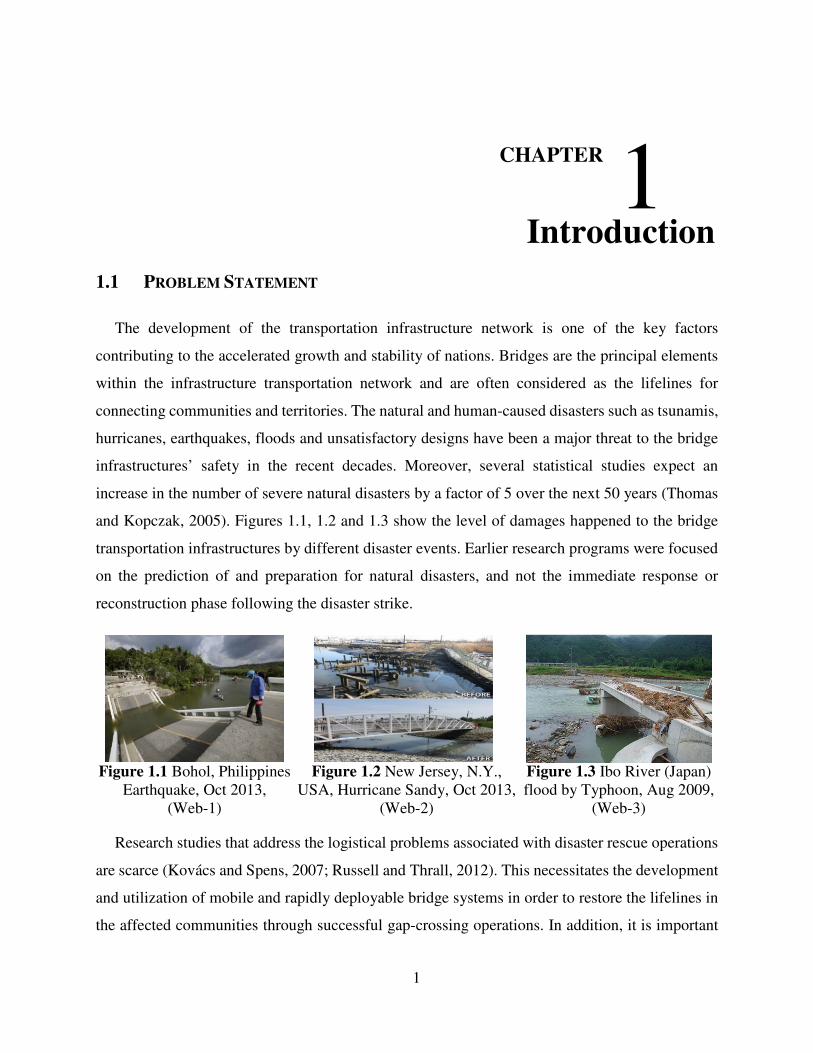
and Kopczak, 2005). Figures 1.1, 1.2 and 1.3 show the level of damages happened to the bridge
transportation infrastructures by different disaster events. Earlier research programs were focused
on the prediction of and preparation for natural disasters, and not the immediate response or
reconstruction phase following the disaster strike.
Figure 1.1 Bohol, Philippines Earthquake, Oct 2013,
(Web-1)
Figure 1.2 New Jersey, N.Y., USA, Hurricane Sandy, Oct 2013,
(Web-2)
Figure 1.3 Ibo River (Japan) flood by Typhoon, Aug 2009,
(Web-3)
Research studies that address the logistical problems associated with disaster rescue operations
are scarce (Kovács and Spens, 2007; Russell and Thrall, 2012). This necessitates the development
and utilization of mobile and rapidly deployable bridge systems in order to restore the lifelines in
the affected communities through successful gap-crossing operations. In addition, it is important
1
2
to mention that the rehabilitation of the damaged bridge infrastructure consumes a long period of
time before being able to restore its serviceability to the transportation network.
1.2 RESEARCH SIGNIFICANCE AND MOTIVATION
The significance of the damage caused by natural disasters to the bridges infrastructure and
post rescue efforts are presented herein through particularly highlighting three disaster events in
the past two decades. The Indian Ocean tsunami (2004) had destroyed hundreds of bridges and
roads for a large distance of kilometers near Banda Aceh, Indonesia. A considerable number of
these bridges were vital links to population mass centers and industrial areas. The disruption
caused to the transportation industry severely constrained the rescue efforts (Cluff, 2007;
Saatcioglu et al., 2006). The Hurricane Katrina (2005) hit three different states in the USA causing
a damage to 44 bridges, five out of which were completely damaged, the rest of the bridges had
different levels of damages, where 20 bridges were severely damaged, 10 bridges were moderately
damaged, and 9 bridges were affected with a low level of damage. Hurricane Mitch (1998) was
more destructive, the hurricane affected three countries in Central America (i.e. Honduras, Costa
Rica, and Nicaragua). In Honduras, 70-80% of the transportation infrastructure was washed out
including 98 bridges, as a result, the air rescue had been used. In Costa Rica, 192 bridges and 800
miles of roads were damaged and wiped out. In Nicaragua 92 bridges were washed out and 70%
of roads’ network could not be accessed (NOAA, 1998).
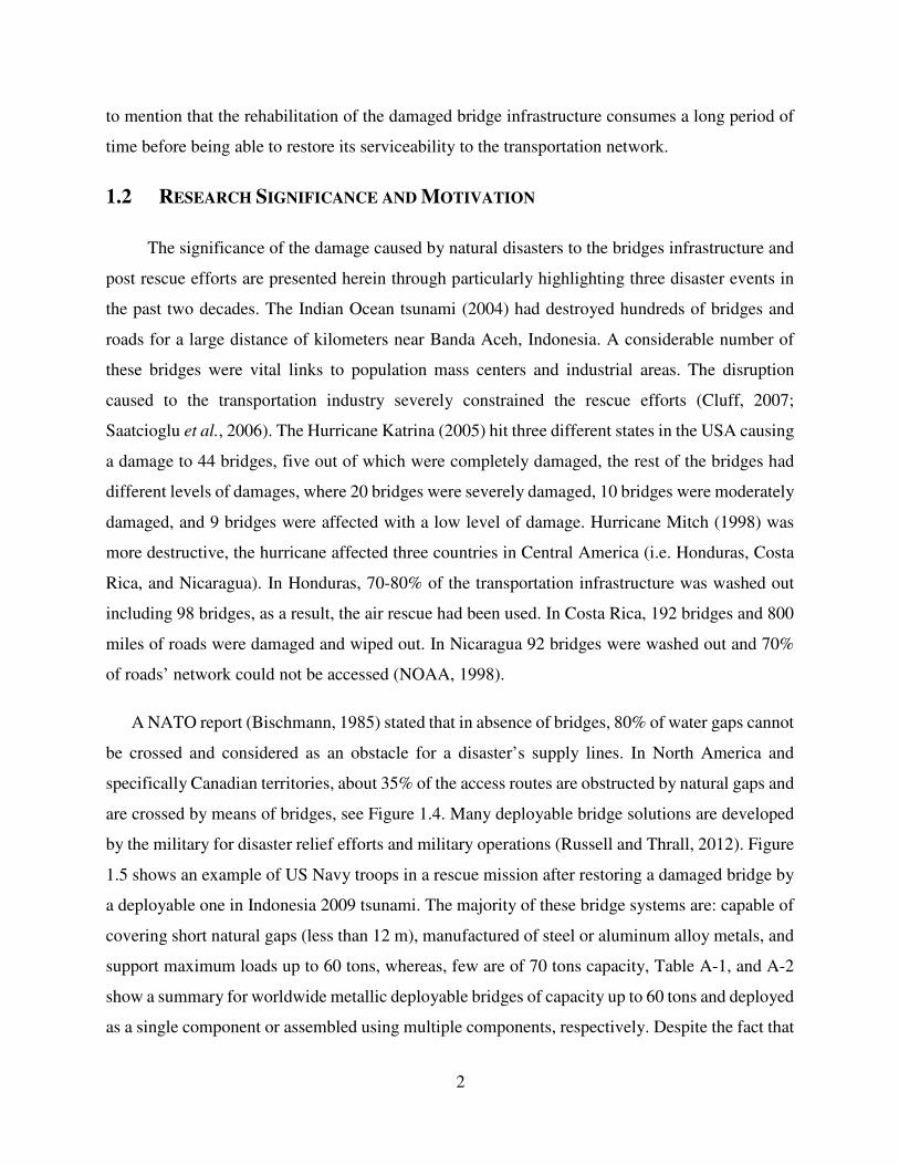
A NATO report (Bischmann, 1985) stated that in absence of bridges, 80% of water gaps cannot
be crossed and considered as an obstacle for a disaster’s supply lines. In North America and
specifically Canadian territories, about 35% of the access routes are obstructed by natural gaps and
are crossed by means of bridges, see Figure 1.4. Many deployable bridge solutions are developed
by the military for disaster relief efforts and military operations (Russell and Thrall, 2012). Figure
1.5 shows an example of US Navy troops in a rescue mission after restoring a damaged bridge by
a deployable one in Indonesia 2009 tsunami. The majority of these bridge systems are: capable of
covering short natural gaps (less than 12 m), manufactured of steel or aluminum alloy metals, and
support maximum loads up to 60 tons, whereas, few are of 70 tons capacity, Table A-1, and A-2
show a summary for worldwide metallic deployable bridges of capacity up to 60 tons and deployed
as a single component or assembled using multiple components, respectively. Despite the fact that
3
a considerable percentage of the natural gaps are less than 12 m span (Kosmatka et al., 2000) (e.g.
over 92% in central Europe and over 51% in Southeast Asia), see Figure 1.4., Comprehensive
studies by Below (2003), Bischmann (1985), Repetski (2003), and Siegel (2000) on the deployable
bridge systems’ requirements illustrate the need of a bridge solution that is capable of covering at
least 20m spans. Satisfying this requirement, supply lifelines to the vital areas will be accessible
in the aftermath of natural disasters at Northeast, Northwest and Central Asia. Furthermore, the
majority of the existing metallic bridge systems are approaching the end of their service life
(Kosmatka, 2011). Any plans to increase the loading capacity of the existing deployable bridges
to meet the recent increase in vehicle loads (i.e. 100 tons) would sacrifice the ease of its mobility,
when considering the fact that deployable bridges are transported by means of tracked, truck
vehicles, and helicopter carriers, see Figures 1.6.a, 1.6.b, and 1.6.c. Therefore, a system with
versatile span coverage, light weight, and high loading capacity is much efficient and more
recommended.
Figure 1.4 Crossing spans percentage of natural gaps’ in different territories
All the aforementioned setbacks (i.e. limited deployable bridges span coverage, end of bridge
systems service life, and achieve an acceptable loading capacity while obtaining a light weight
bridge for rapid mobility) cast doubts on the effectiveness of deployable bridge solutions and
increase the difficulty of such structure’s design. Therefore, in order to achieve an effective
0.30.6 1.5 2.6
2.7
92.3
more than 157 feet132-157 feet24-39.3 m18-23.7 m12 -17.7 mLess than 12 m
30
1951
18-23.7 m
12-17.7 m
Less than 12 m
About 35% of the transportation network bidges are of short span
Europe
Asia
North America
4
deployable bridge system which facilitates saving human beings’ lives during post-disaster rescue
efforts, three significant factors have to be considered. These factors are: light weight and high
strength material for the bridge shall be used (i.e. fiber composite laminates), The use of a bridge
modular unit that is commonly utilized to form a family of bridges for covering different spans,
and finally the design process of such bridges must be optimized to reach an optimally minimized
weight to loading capacity ratio.
(a) Resuce aids by tracked vehicle carriers, (Coker, 2009)
(b) Resuce aids by truck carriers (Coker, 2009)
(c) Resuce aids by Heliocopter carriers, (Coker, 2009)
Figure 1.6 Methods of deployable bridges mobility
Different structural shapes of bridge deployment systems have been used in the past decades.
For instance, bridges that have used the truss shaped design such as:
a) The Medium Girder Bridge (MGB) that was manufactured of a modular trussed shape system.
The bridge can be erected in several stories to cover versatile spans, from 9.9m to 45.8 m span,
however, its main setback is the high number of manpower needed for the deployment
operation and a relatively increased deployment time, about 90 min.(Coker, 2009),
Figure 1.5 Bridge destroyed in a tsunami near Banda Aceh, Jan 2005,.Sumatra, Indonesia
(U.S. Navy, 2005)
5
b) The Tied Assault Truss Bridge (TATB) which is composed of tied arch structural folded units
made of aluminum alloy. The system provides a fast deployment in minimal time. On the other
hand, it is constrained to a fixed span coverage of 12m (Thomas and Sia, 2013).
Another type of deployable bridge systems used the arched structural design such as: a) the
Churchill, A22 bridge layer, and b) the Composite Assault Bridge (CAB) (Kosmatka et al., 2000).
The arched system provides an efficient load distribution over the bridge deck with no stress
concentration points. However, its deficiency is the fixed span coverage. A third type of bridges
have used the tapered shape design such as: a) the Heavy Assault Bridge (HAB) system (kerr,
1990), and b) the scissors deployment system of the Armored Vehicle Launched Bridge (AVLB)
(Russell and Thrall, 2012). Although these systems are characterized by ease of deployment but
again they have a limited span coverage. Finally, the bridge systems composed of beam modular
units are characterized by low bridge profile, ease of assembly to cover multiple spans and can be
functional in conjunction with different systems to cross wet or dry gaps like the Light-weight
Causeway bridge System (LMCS) (Russell and Thrall, 2012) and the Dry Support Bridge (DSB),
(Coker, 2009), respectively, in particular, the LMCS consists of aluminum Treadway beams
supported over pneumatic floats. The bridge beam modular units are typically manufactured from
metals, aluminum alloy or steel, which have relatively heavy weight and less strength when
compared to fiber composite laminates. Therefore, the focus of this research is to investigate the
reliability of using composites for the deployable bridge beam design, and to develop an innovative
deck core configuration for the light weight mobility of these bridges. The design and analysis of
deployable bridge structural components in this study complies with the Trilateral Design and Test
Code for Military Bridging and Gap Crossing Equipment (TDTC, 2005). This code is different
from the commonly used design codes for the civilian bridges, such as ASHTOO and CHBDC
…etc. The TDTC does not impose a serviceability limit for the sake of more structural weight
reduction as opposed to the other design codes. The design loads in the TDTC are very high and
the axle loads spacing are very small. For instance, most of the existing deployable bridge have a
carrying capacity of 600 kN or higher, a hypothetical vehicle of Military Loading Class of 600 kN
(MLC60) has axle loads distributed over 10.97 m for a wheeled truck or 4.27 m for a tracked
vehicle, whereas, in CHBDC the hypothetical wheeled vehicle CL-625 is used for the maximum
case of loading in the bridge design which has a weight of 625 kN and the axle loads are spaced
over 18 m vehicle length. In TDTC, the bridge structure and connections design has to sustain
6
different severe loading conditions during launching and retrieval as well as the stresses induced
due to the passing vehicle loads, which is a not a similar case in the design of civilian bridges
where mostly the bridge is constructed in the site over the crossed gap. Deployable bridges
designed using the TDTC code provisions are only simply supported over the home and far banks;
no fixation or anchorage mostly to the bank soil is considered. Moreover, the design has to take
into account the slope, and height difference between bank conditions, in civilian bridges the banks
has to be well leveled with adequate bearing capacity to carry the bridge support reactions.
Composite laminate structural elements are characterized by a large number of design
parameters that can be implemented in the design of bridge beams to reach an optimal weight
design and acceptable capacity, (i.e. ply orientation, stacking sequence, elements surface
dimensionality and elements thicknesses…etc.). Moreover, optimizing the design parameters of
the bridge beam geometry would lead to an optimal composite laminate stress distribution, hence,
minimizing the bridge weight. Therefore, the design optimization of such bridge systems may
seem to be advantageous for achieving an effective deployable bridge system and saving peoples'
lives in the post-disaster rescue efforts.
The use of any optimization technique for an effective structural design optimization is not
generic. In other words, no optimization algorithm can possibly be effective or even successful for
all cases of interest. The physical problem’s nature and field of application have a significant
influence on the suitability and efficiency of different optimization algorithms (Das & Suganthan,
2011; Aimin Zhou et al., 2011). Therefore, this research study is motivated to develop a proper
and competitive algorithm for design optimization of large scale structures and composite mobile
bridge systems.
Figure 1.7 Elements for a typical deployable and mobile tread-way bridge beams system (Robinson, 2008)
(c) Ramp module (b) bridge beam
(a) Deck section
7
1.3 OBJECTIVES AND SCOPE OF WORK
In order to meet the needs of light weight bridging in the aftermath of natural disasters, This
research study aims to: develop a novel light weight sandwich core configurations to act as the
compression bearing element of a bridge beam like structure, and use an effective structural design
optimization metaheuristic approach to enhance the designed cores performance. In order to
achieve these objectives the following goals are set:
• Design and develop light weight sandwich cores for the composite deployable bridge decks.
• Propose an effective optimization algorithm for design optimization of complex and large-
scale structures.
• Increase the composite deployable bridge capacity/weight ratio by maximizing the
compression and shear strength of the developed light-weight sandwich cores.
The scope of work can be divided into two parts. The first part can be summarized as follows:
• Evaluate different well-known swarm intelligence algorithms presented in the literature for the
application of complex structure optimization.
• Based on this evaluation, propose a new method to enhance the candidate algorithm
performance, i.e. Particle Swarm Optimization (PSO), and minimize to a considerable level
it`s deficiency to structural optimization.
• Further, hybridize the modified swarm intelligence optimizer with Response Surface
Methodology (RSM) as a tool to distinguish the influence level of design parameters in
complex structural models.
• Create a discrete version of the developed algorithm and merge a studied technique for
redirecting the design points to feasible regions.
• Re-formulate the discrete version of the algorithm to suite the discrete design nature of
composite laminate structural optimization problems.
Whereas, the scope of the second part can be summarized as follows:
• Design and develop an innovative light weight sandwich composite cores for the bridge beam
deck with high compressive and shear capacity,
• Conduct experimental testing to quantify the compression, and shear capacity of the developed
sandwich cores.

8
• Numerically investigate the progressive compression, and shear failure of the designed cores.
• Validate the numerical models’ results of the sandwich composite cores with the experimental
results.
• Use the discrete version of the developed optimization algorithm to enhance the sandwich
cores compression and shear capacity and compare it to the base design.
9
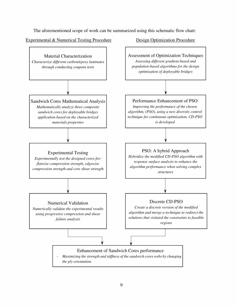
The aforementioned scope of work can be summarized using this schematic flow chart:
Experimental & Numerical Testing Procedure Design Optimization Procedure
Material Characterization Characterize different carbon/epoxy laminates
through conducting coupons tests
Sandwich Cores Mathematical Analysis Mathematically analyze three composite
sandwich cores for deployable bridges
application based on the characterized
materials properties
Experimental Testing Experimentally test the designed cores for:
flatwise compression strength, edgewise
compression strength and core shear strength
Numerical Validation Numerically validate the experimental results
using progressive compression and shear
failure analysis
Enhancement of Sandwich Cores performance - Maximizing the strength and stiffness of the sandwich cores webs by changing
the ply orientation.
Assessment of Optimization Techniques Assessing different gradient-based and
population-based algorithms for the design
optimization of deployable bridges
Performance Enhancement of PSO Improving the performance of the chosen
algorithm, (PSO), using a new diversity control
technique for continuous optimization, CD-PSO
is developed
PSO: A hybrid Approach Hybridize the modified CD-PSO algorithm with
response surface analysis to enhance the
algorithm performance when solving complex
structures
Discrete CD-PSO Create a discrete version of the modified
algorithm and merge a technique to redirect the
solutions that violated the constraints to feasible
regions
10
1.4 THESIS LAYOUT
This thesis contributes to the state of the art of deployable bridges used for rapid post-disaster
mobility and proposes a methodology for achieving an effective deployable bridge system that is
competitive with the recently developed in mobile bridges industry. The thesis is composed of
seven chapters. The Introduction chapter is followed by Chapter 2 that includes literature survey
of the existing deployable bridge systems used for disaster relief operations, followed by a
representation that focuses on the mobile bridges fabricated of composites laminates and the recent
research studies on enhancing the weight to capacity ratio of these bridges. Description of the
effectiveness of structural design optimization for deployable bridges will be presented in Chapter
3. The chapter is dedicated to the assessment of different optimization algorithms to select the
most effective one for bridge design optimization and concluded to a candidate optimization
algorithm, i.e. PSO. Chapter 4 describes the newly developed optimization algorithm mechanism
and discusses the evaluation of the algorithm’s performance through the application over
benchmark structures and large-scale deployable bridge system. Chapter 5 presents different
sandwich core configurations that are designed to increase the loading capacity of the deployable
bridge treadways, followed by explanation of three different test setups and their instrumentations.
The experiments objective is to evaluate the cores’ compression and shear capacity. Finally, a
numerical validation of the experimental results is conducted to assess the models’ reliability for
testing more complex sandwich cores. Chapter 6 presents the PSO discrete approach for
maximizing the strength of the composite laminates and discusses the enhancement achieved by
its application on the designed sandwich cores. Last chapter, Chapter 7, presents the conclusions
and summary of the design recommendation for designing the sandwich cores in addition to the
future work.
11
CHAPTER 2
Literature Review 2.1 INTRODUCTION
The increasing rate of the world natural disasters emphasized the importance of rapid mobility.
Within the past decades, the deployable bridge systems developed by various military armies were
the mostly used ones for the post-disaster relief operations. Recently, research efforts started to
focus on approaching an effective deployable bridge system in terms of lightweight and high
capacity. In this chapter, a detailed review of the in-service armies’ metallic deployable and mobile
bridge solutions will be presented, followed by a survey of the research conducted for developing
composite deployable bridge structure. The chapter ends with a summary of the literature related
to optimization of deployable bridges and composite laminates.
2.2 MILITARY BRIDGE SOLUTIONS
Military bridges differ from the traditional bridges connecting the public transportation network
in terms of mobility, method of erection and placement. The rapid mobility requirement for
military bridges limits their material weight and erection method. The infield damage repair for
the military bridges is not practical. Therefore, they are manufactured of multiple modular units
that can be easily assembled together or replaced in a minimal time. For the aforementioned
reasons, an effective deployable and mobile bridge system shall be characterized by a minimum
weight to bearing capacity ratio as well as a quick launching and retrieval assembly.
The military deployable bridge solutions can be classified into three categories based on their
mission purpose in the military doctrine. These categories are: Assault bridge solutions, Tactical
bridge solutions and Line of communication bridge solutions. The assault bridge solutions are
temporary bridges that are designed for gap crossing of the leading troops as rapidly as possible to
the front lines. The coverage span of the assault bridges is typically less than 25 m. The tactical
bridge solutions are used to cover wider spans up to 40 m and to replace the assault bridges that
are required to other gap crossings. The line of communication (LOC) bridges are designed for the
long-term use and used to be placed aside to the tactical bridges or to replace them. The LOC
2
12
bridges can cover any desired span using abutments. A brief description of seven bridge solutions
of the categories that are widely used in post-disaster relief, namely: Assault Bridges and Tactical
Bridges, will be presented in the following subsections.
2.2.1 ASSAULT BRIDGE SYSTEMS
I. Close Support Bridge (BR-90)
The Close Support Bridge (CSB) is manufactured by BAE Defense Systems co. (Vickers co.)
to serve in the British Royal Army. The CSB system is produced in three classes (i.e. No.10, No.11,
and No.12), the three classes are capable of supporting spans of 24.5, 14.5, and 12 m, respectively.
The system can be launched by an Automotive Bridge Launching Equipment (ABLE) that is
equipped with a crane and assembly platform, or the system can be mounted on a tank and launched
by a mechanical system. The Bridge system consists of multiple internal modular units of 1m depth
and ramp modules for the end supports. A modular bridge unit is in the shape of the two
interconnecting treadway beams that forms one lane with width 4m. The Bridge has a Military
Loading Class of MLC70 (i.e. 70 tons) for tanks crossing and MLC100 (i.e.100 tons) for wheeled
trucks. The system is made of lightweight Aluminum alloy material, therefore, the time of
launching and retrieval is 10 minutes for its shortest class, No.12, which has a weight of 5,445 kg.
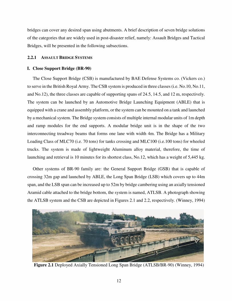
Other systems of BR-90 family are: the General Support Bridge (GSB) that is capable of
crossing 32m gap and launched by ABLE, the Long Span Bridge (LSB) which covers up to 44m
span, and the LSB span can be increased up to 52m by bridge cambering using an axially tensioned
Aramid cable attached to the bridge bottom, the system is named, ATLSB. A photograph showing
the ATLSB system and the CSB are depicted in Figures 2.1 and 2.2, respectively. (Winney, 1994)
Figure 2.1 Deployed Axially Tensioned Long Span Bridge (ATLSB/BR-90) (Winney, 1994)
13
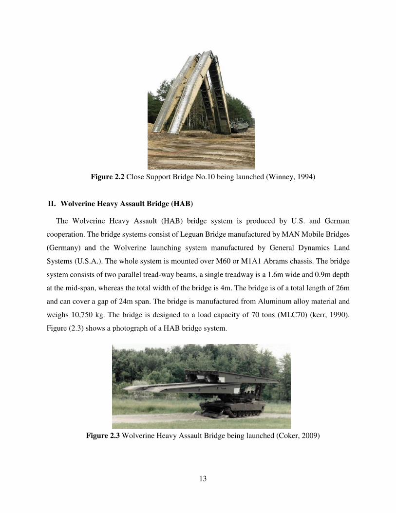
Figure 2.2 Close Support Bridge No.10 being launched (Winney, 1994)
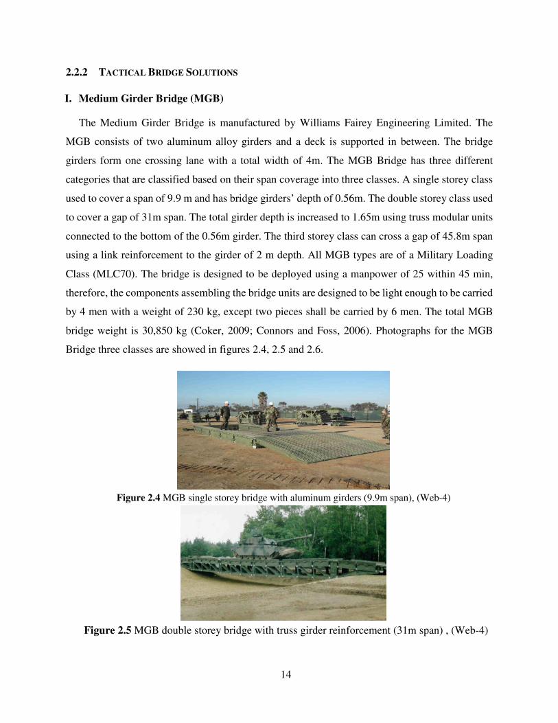
II. Wolverine Heavy Assault Bridge (HAB)
The Wolverine Heavy Assault (HAB) bridge system is produced by U.S. and German
cooperation. The bridge systems consist of Leguan Bridge manufactured by MAN Mobile Bridges
(Germany) and the Wolverine launching system manufactured by General Dynamics Land
Systems (U.S.A.). The whole system is mounted over M60 or M1A1 Abrams chassis. The bridge
system consists of two parallel tread-way beams, a single treadway is a 1.6m wide and 0.9m depth
at the mid-span, whereas the total width of the bridge is 4m. The bridge is of a total length of 26m
and can cover a gap of 24m span. The bridge is manufactured from Aluminum alloy material and
weighs 10,750 kg. The bridge is designed to a load capacity of 70 tons (MLC70) (kerr, 1990).
Figure (2.3) shows a photograph of a HAB bridge system.
Figure 2.3 Wolverine Heavy Assault Bridge being launched (Coker, 2009)
14
2.2.2 TACTICAL BRIDGE SOLUTIONS
I. Medium Girder Bridge (MGB)
The Medium Girder Bridge is manufactured by Williams Fairey Engineering Limited. The
MGB consists of two aluminum alloy girders and a deck is supported in between. The bridge
girders form one crossing lane with a total width of 4m. The MGB Bridge has three different
categories that are classified based on their span coverage into three classes. A single storey class
used to cover a span of 9.9 m and has bridge girders’ depth of 0.56m. The double storey class used
to cover a gap of 31m span. The total girder depth is increased to 1.65m using truss modular units
connected to the bottom of the 0.56m girder. The third storey class can cross a gap of 45.8m span
using a link reinforcement to the girder of 2 m depth. All MGB types are of a Military Loading
Class (MLC70). The bridge is designed to be deployed using a manpower of 25 within 45 min,
therefore, the components assembling the bridge units are designed to be light enough to be carried
by 4 men with a weight of 230 kg, except two pieces shall be carried by 6 men. The total MGB
bridge weight is 30,850 kg (Coker, 2009; Connors and Foss, 2006). Photographs for the MGB
Bridge three classes are showed in figures 2.4, 2.5 and 2.6.
Figure 2.4 MGB single storey bridge with aluminum girders (9.9m span), (Web-4)
Figure 2.5 MGB double storey bridge with truss girder reinforcement (31m span) , (Web-4)
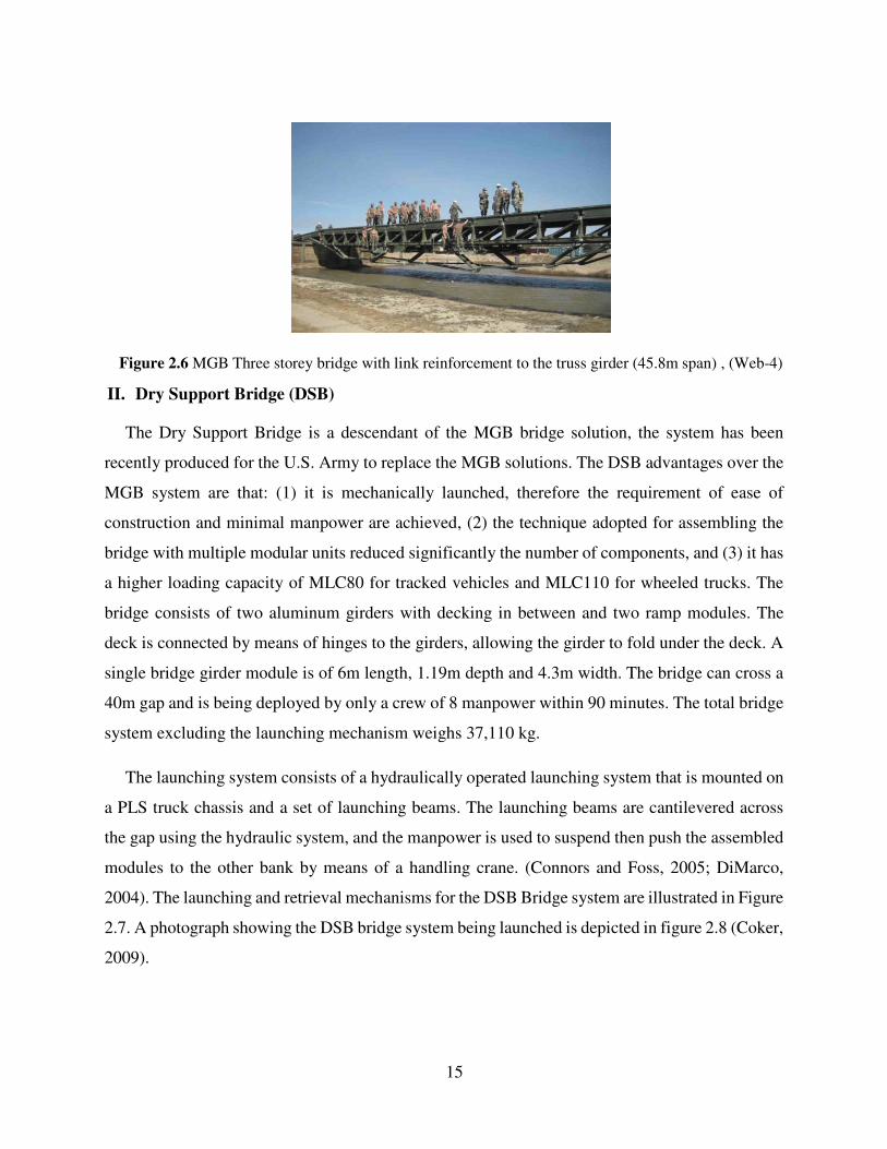
15
Figure 2.6 MGB Three storey bridge with link reinforcement to the truss girder (45.8m span) , (Web-4)
II. Dry Support Bridge (DSB)
The Dry Support Bridge is a descendant of the MGB bridge solution, the system has been
recently produced for the U.S. Army to replace the MGB solutions. The DSB advantages over the
MGB system are that: (1) it is mechanically launched, therefore the requirement of ease of
construction and minimal manpower are achieved, (2) the technique adopted for assembling the
bridge with multiple modular units reduced significantly the number of components, and (3) it has
a higher loading capacity of MLC80 for tracked vehicles and MLC110 for wheeled trucks. The
bridge consists of two aluminum girders with decking in between and two ramp modules. The
deck is connected by means of hinges to the girders, allowing the girder to fold under the deck. A
single bridge girder module is of 6m length, 1.19m depth and 4.3m width. The bridge can cross a
40m gap and is being deployed by only a crew of 8 manpower within 90 minutes. The total bridge
system excluding the launching mechanism weighs 37,110 kg.
The launching system consists of a hydraulically operated launching system that is mounted on
a PLS truck chassis and a set of launching beams. The launching beams are cantilevered across
the gap using the hydraulic system, and the manpower is used to suspend then push the assembled
modules to the other bank by means of a handling crane. (Connors and Foss, 2005; DiMarco,
2004). The launching and retrieval mechanisms for the DSB Bridge system are illustrated in Figure
2.7. A photograph showing the DSB bridge system being launched is depicted in figure 2.8 (Coker,
2009).
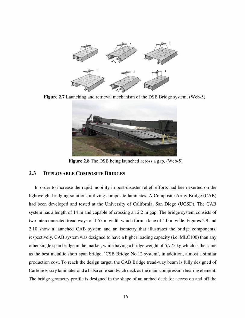
16
Figure 2.7 Launching and retrieval mechanism of the DSB Bridge system, (Web-5)
Figure 2.8 The DSB being launched across a gap, (Web-5)
2.3 DEPLOYABLE COMPOSITE BRIDGES
In order to increase the rapid mobility in post-disaster relief, efforts had been exerted on the
lightweight bridging solutions utilizing composite laminates. A Composite Army Bridge (CAB)
had been developed and tested at the University of California, San Diego (UCSD). The CAB
system has a length of 14 m and capable of crossing a 12.2 m gap. The bridge system consists of
two interconnected tread ways of 1.55 m width which form a lane of 4.0 m wide. Figures 2.9 and
2.10 show a launched CAB system and an isometry that illustrates the bridge components,
respectively. CAB system was designed to have a higher loading capacity (i.e. MLC100) than any
other single span bridge in the market, while having a bridge weight of 5,775 kg which is the same
as the best metallic short span bridge, ’CSB Bridge No.12 system’, in addition, almost a similar
production cost. To reach the design target, the CAB Bridge tread-way beam is fully designed of
Carbon/Epoxy laminates and a balsa core sandwich deck as the main compression bearing element.
The bridge geometry profile is designed in the shape of an arched deck for access on and off the
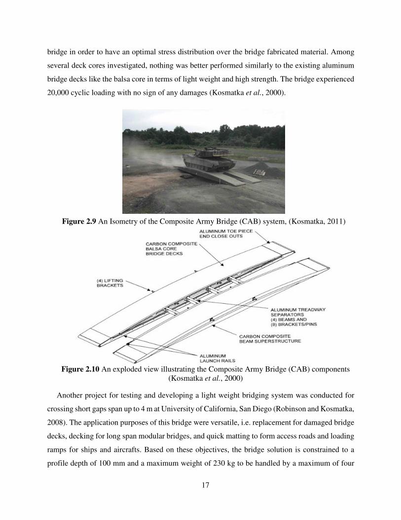
17
bridge in order to have an optimal stress distribution over the bridge fabricated material. Among
several deck cores investigated, nothing was better performed similarly to the existing aluminum
bridge decks like the balsa core in terms of light weight and high strength. The bridge experienced
20,000 cyclic loading with no sign of any damages (Kosmatka et al., 2000).
Figure 2.9 An Isometry of the Composite Army Bridge (CAB) system, (Kosmatka, 2011)
Figure 2.10 An exploded view illustrating the Composite Army Bridge (CAB) components
(Kosmatka et al., 2000)
Another project for testing and developing a light weight bridging system was conducted for
crossing short gaps span up to 4 m at University of California, San Diego (Robinson and Kosmatka,
2008). The application purposes of this bridge were versatile, i.e. replacement for damaged bridge
decks, decking for long span modular bridges, and quick matting to form access roads and loading
ramps for ships and aircrafts. Based on these objectives, the bridge solution is constrained to a
profile depth of 100 mm and a maximum weight of 230 kg to be handled by a maximum of four
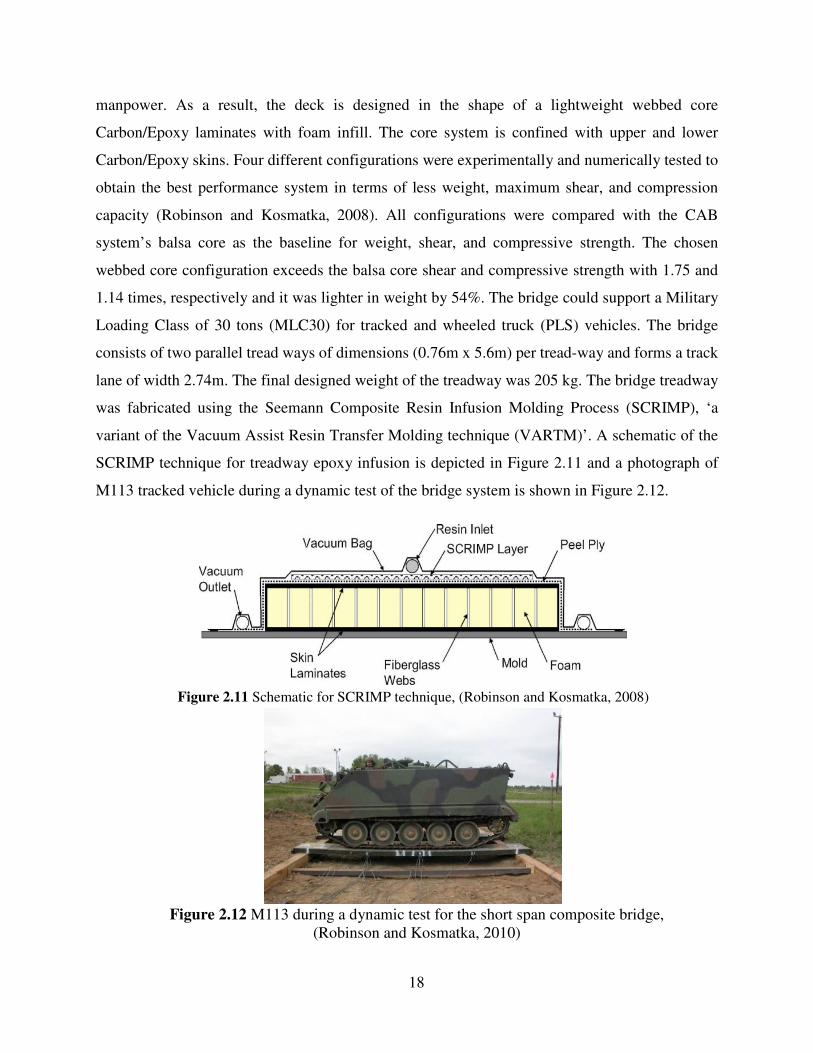
18
manpower. As a result, the deck is designed in the shape of a lightweight webbed core
Carbon/Epoxy laminates with foam infill. The core system is confined with upper and lower
Carbon/Epoxy skins. Four different configurations were experimentally and numerically tested to
obtain the best performance system in terms of less weight, maximum shear, and compression
capacity (Robinson and Kosmatka, 2008). All configurations were compared with the CAB
system’s balsa core as the baseline for weight, shear, and compressive strength. The chosen
webbed core configuration exceeds the balsa core shear and compressive strength with 1.75 and
1.14 times, respectively and it was lighter in weight by 54%. The bridge could support a Military
Loading Class of 30 tons (MLC30) for tracked and wheeled truck (PLS) vehicles. The bridge
consists of two parallel tread ways of dimensions (0.76m x 5.6m) per tread-way and forms a track
lane of width 2.74m. The final designed weight of the treadway was 205 kg. The bridge treadway
was fabricated using the Seemann Composite Resin Infusion Molding Process (SCRIMP), ‘a
variant of the Vacuum Assist Resin Transfer Molding technique (VARTM)’. A schematic of the
SCRIMP technique for treadway epoxy infusion is depicted in Figure 2.11 and a photograph of
M113 tracked vehicle during a dynamic test of the bridge system is shown in Figure 2.12.
Figure 2.11 Schematic for SCRIMP technique, (Robinson and Kosmatka, 2008)
Figure 2.12 M113 during a dynamic test for the short span composite bridge,
(Robinson and Kosmatka, 2010)
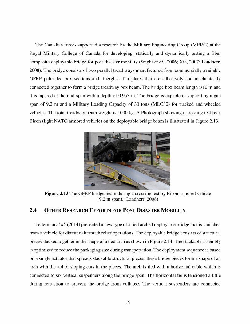
19
The Canadian forces supported a research by the Military Engineering Group (MERG) at the
Royal Military College of Canada for developing, statically and dynamically testing a fiber
composite deployable bridge for post-disaster mobility (Wight et al., 2006; Xie, 2007; Landherr,
2008). The bridge consists of two parallel tread ways manufactured from commercially available
GFRP pultruded box sections and fiberglass flat plates that are adhesively and mechanically
connected together to form a bridge treadway box beam. The bridge box beam length is10 m and
it is tapered at the mid-span with a depth of 0.953 m. The bridge is capable of supporting a gap
span of 9.2 m and a Military Loading Capacity of 30 tons (MLC30) for tracked and wheeled
vehicles. The total treadway beam weight is 1000 kg. A Photograph showing a crossing test by a
Bison (light NATO armored vehicle) on the deployable bridge beam is illustrated in Figure 2.13.
Figure 2.13 The GFRP bridge beam during a crossing test by Bison armored vehicle
(9.2 m span), (Landherr, 2008)
2.4 OTHER RESEARCH EFFORTS FOR POST DISASTER MOBILITY
Lederman et al. (2014) presented a new type of a tied arched deployable bridge that is launched
from a vehicle for disaster aftermath relief operations. The deployable bridge consists of structural
pieces stacked together in the shape of a tied arch as shown in Figure 2.14. The stackable assembly
is optimized to reduce the packaging size during transportation. The deployment sequence is based
on a single actuator that spreads stackable structural pieces; these bridge pieces form a shape of an
arch with the aid of sloping cuts in the pieces. The arch is tied with a horizontal cable which is
connected to six vertical suspenders along the bridge span. The horizontal tie is tensioned a little
during retraction to prevent the bridge from collapse. The vertical suspenders are connected
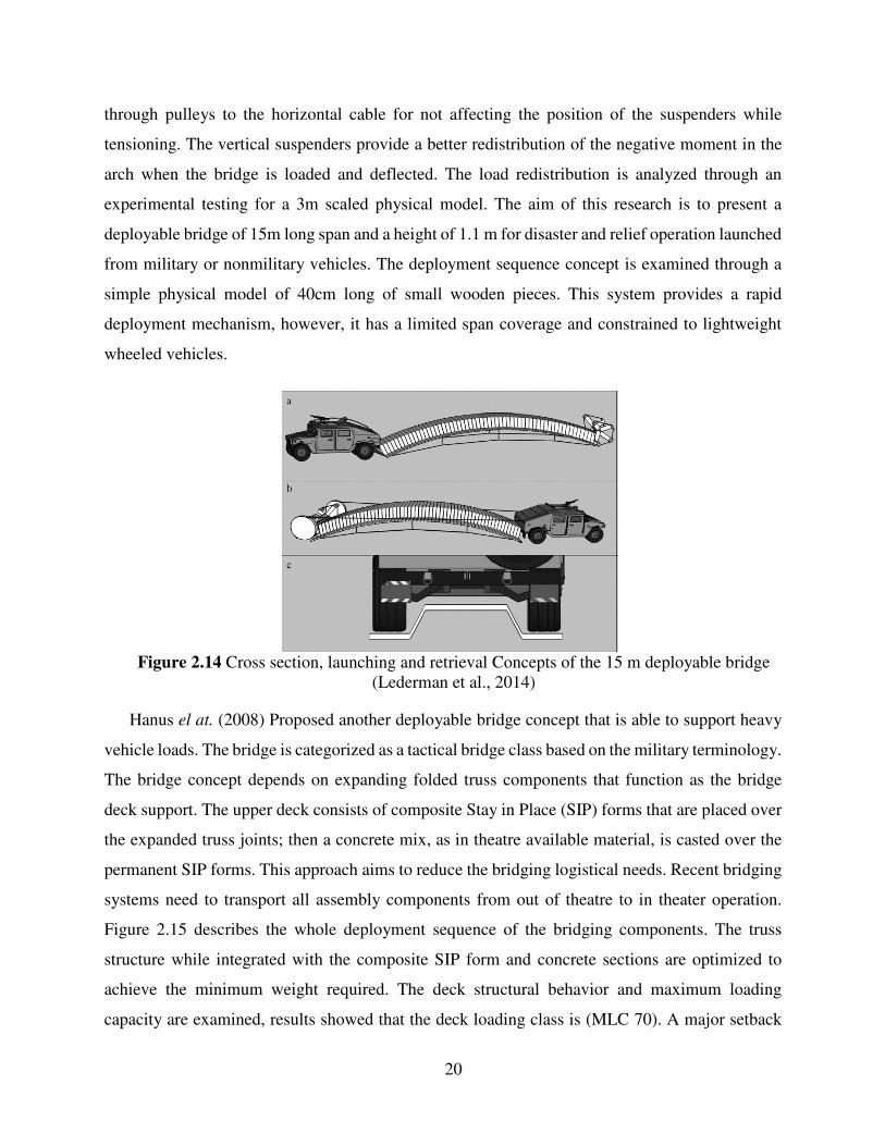
20
through pulleys to the horizontal cable for not affecting the position of the suspenders while
tensioning. The vertical suspenders provide a better redistribution of the negative moment in the
arch when the bridge is loaded and deflected. The load redistribution is analyzed through an
experimental testing for a 3m scaled physical model. The aim of this research is to present a
deployable bridge of 15m long span and a height of 1.1 m for disaster and relief operation launched
from military or nonmilitary vehicles. The deployment sequence concept is examined through a
simple physical model of 40cm long of small wooden pieces. This system provides a rapid
deployment mechanism, however, it has a limited span coverage and constrained to lightweight
wheeled vehicles.
Figure 2.14 Cross section, launching and retrieval Concepts of the 15 m deployable bridge
(Lederman et al., 2014)
Hanus el at. (2008) Proposed another deployable bridge concept that is able to support heavy
vehicle loads. The bridge is categorized as a tactical bridge class based on the military terminology.
The bridge concept depends on expanding folded truss components that function as the bridge
deck support. The upper deck consists of composite Stay in Place (SIP) forms that are placed over
the expanded truss joints; then a concrete mix, as in theatre available material, is casted over the
permanent SIP forms. This approach aims to reduce the bridging logistical needs. Recent bridging
systems need to transport all assembly components from out of theatre to in theater operation.
Figure 2.15 describes the whole deployment sequence of the bridging components. The truss
structure while integrated with the composite SIP form and concrete sections are optimized to
achieve the minimum weight required. The deck structural behavior and maximum loading
capacity are examined, results showed that the deck loading class is (MLC 70). A major setback
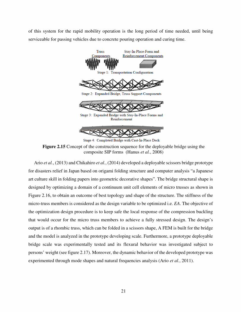
21
of this system for the rapid mobility operation is the long period of time needed, until being
serviceable for passing vehicles due to concrete pouring operation and curing time.
Figure 2.15 Concept of the construction sequence for the deployable bridge using the
composite SIP forms (Hanus et al., 2008)
Ario et al., (2013) and Chikahiro et al., (2014) developed a deployable scissors bridge prototype
for disasters relief in Japan based on origami folding structure and computer analysis “a Japanese
art culture skill in folding papers into geometric decorative shapes”. The bridge structural shape is
designed by optimizing a domain of a continuum unit cell elements of micro trusses as shown in
Figure 2.16, to obtain an outcome of best topology and shape of the structure. The stiffness of the
micro-truss members is considered as the design variable to be optimized i.e. EA. The objective of
the optimization design procedure is to keep safe the local response of the compression buckling
that would occur for the micro truss members to achieve a fully stressed design. The design’s
output is of a rhombic truss, which can be folded in a scissors shape, A FEM is built for the bridge
and the model is analyzed in the prototype developing scale. Furthermore, a prototype deployable
bridge scale was experimentally tested and its flexural behavior was investigated subject to
persons’ weight (see figure 2.17). Moreover, the dynamic behavior of the developed prototype was
experimented through mode shapes and natural frequencies analysis (Ario et al., 2011).
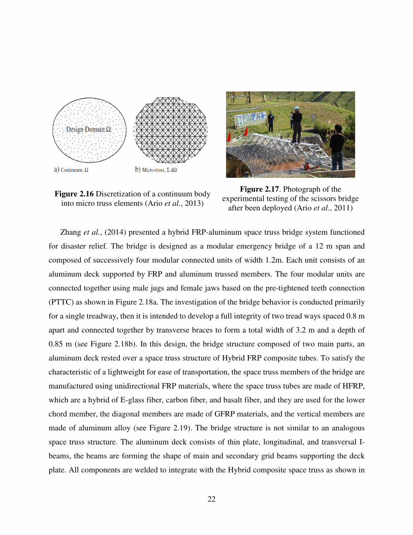
22
Figure 2.16 Discretization of a continuum body into micro truss elements (Ario et al., 2013)
Figure 2.17. Photograph of the experimental testing of the scissors bridge
after been deployed (Ario et al., 2011)
Zhang et al., (2014) presented a hybrid FRP-aluminum space truss bridge system functioned
for disaster relief. The bridge is designed as a modular emergency bridge of a 12 m span and
composed of successively four modular connected units of width 1.2m. Each unit consists of an
aluminum deck supported by FRP and aluminum trussed members. The four modular units are
connected together using male jugs and female jaws based on the pre-tightened teeth connection
(PTTC) as shown in Figure 2.18a. The investigation of the bridge behavior is conducted primarily
for a single treadway, then it is intended to develop a full integrity of two tread ways spaced 0.8 m
apart and connected together by transverse braces to form a total width of 3.2 m and a depth of
0.85 m (see Figure 2.18b). In this design, the bridge structure composed of two main parts, an
aluminum deck rested over a space truss structure of Hybrid FRP composite tubes. To satisfy the
characteristic of a lightweight for ease of transportation, the space truss members of the bridge are
manufactured using unidirectional FRP materials, where the space truss tubes are made of HFRP,
which are a hybrid of E-glass fiber, carbon fiber, and basalt fiber, and they are used for the lower
chord member, the diagonal members are made of GFRP materials, and the vertical members are
made of aluminum alloy (see Figure 2.19). The bridge structure is not similar to an analogous
space truss structure. The aluminum deck consists of thin plate, longitudinal, and transversal I-
beams, the beams are forming the shape of main and secondary grid beams supporting the deck
plate. All components are welded to integrate with the Hybrid composite space truss as shown in
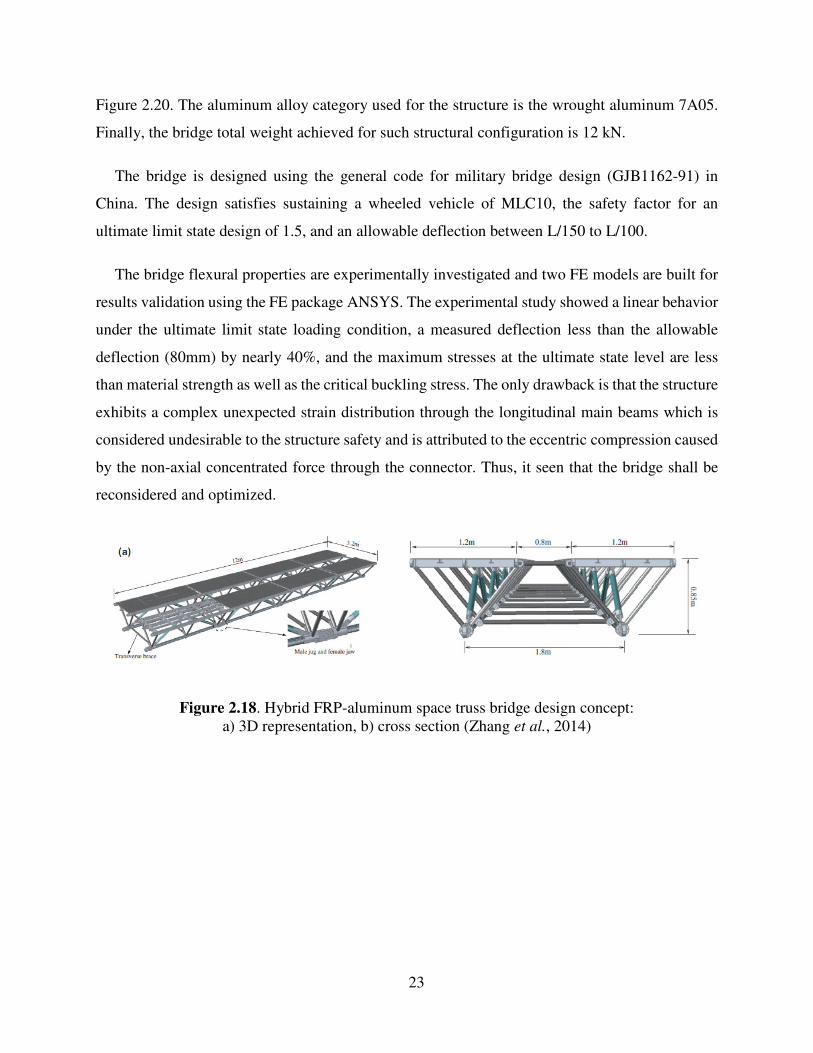
23
Figure 2.20. The aluminum alloy category used for the structure is the wrought aluminum 7A05.
Finally, the bridge total weight achieved for such structural configuration is 12 kN.
The bridge is designed using the general code for military bridge design (GJB1162-91) in
China. The design satisfies sustaining a wheeled vehicle of MLC10, the safety factor for an
ultimate limit state design of 1.5, and an allowable deflection between L/150 to L/100.
The bridge flexural properties are experimentally investigated and two FE models are built for
results validation using the FE package ANSYS. The experimental study showed a linear behavior
under the ultimate limit state loading condition, a measured deflection less than the allowable
deflection (80mm) by nearly 40%, and the maximum stresses at the ultimate state level are less
than material strength as well as the critical buckling stress. The only drawback is that the structure
exhibits a complex unexpected strain distribution through the longitudinal main beams which is
considered undesirable to the structure safety and is attributed to the eccentric compression caused
by the non-axial concentrated force through the connector. Thus, it seen that the bridge shall be
reconsidered and optimized.
Figure 2.18. Hybrid FRP-aluminum space truss bridge design concept: a) 3D representation, b) cross section (Zhang et al., 2014)
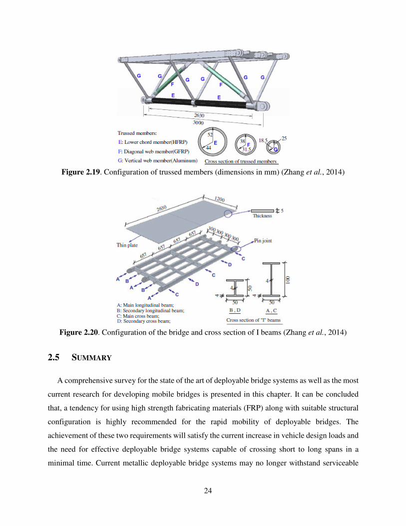
24
Figure 2.19. Configuration of trussed members (dimensions in mm) (Zhang et al., 2014)
Figure 2.20. Configuration of the bridge and cross section of I beams (Zhang et al., 2014)
2.5 SUMMARY
A comprehensive survey for the state of the art of deployable bridge systems as well as the most
current research for developing mobile bridges is presented in this chapter. It can be concluded
that, a tendency for using high strength fabricating materials (FRP) along with suitable structural
configuration is highly recommended for the rapid mobility of deployable bridges. The
achievement of these two requirements will satisfy the current increase in vehicle design loads and
the need for effective deployable bridge systems capable of crossing short to long spans in a
minimal time. Current metallic deployable bridge systems may no longer withstand serviceable

25
for those higher specifications. Most of the current researches that had used metals for deployable
bridges are functioned for covering short gap spans with high vehicle’s capacity, long gap spans
with low vehicle’s capacity, or for the rescue of people in the aftermath of a disaster. Up to the
author’s knowledge, no current research focused on the design optimization of these mobile bridge
structures to achieve higher performance, whereas, some of the current research emphasized the
need of optimizing the deployable bridge structure after it had been studied and developed.
Therefore, the main focus of this study is to propose an effective optimization algorithm for the
design of these type of bridges as well as to develop different FRP sandwich cores capable of
effectively decreasing the weight to capacity ratio of the state of art composite deployable bridges.
Chapter 3 will cover several optimization methods used effectively for structural design
optimization. Based on a literature survey, candidate algorithms implementing different
optimization techniques are applied and tested on a deployable bridge structure of versatile span
coverage. The more effective one is chosen for further investigation and performance
enhancement.
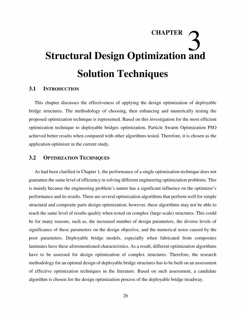
26
CHAPTER 3
Structural Design Optimization and
Solution Techniques 3.1 INTRODUCTION
This chapter discusses the effectiveness of applying the design optimization of deployable
bridge structures. The methodology of choosing, then enhancing and numerically testing the
proposed optimization technique is represented. Based on this investigation for the most efficient
optimization technique to deployable bridges optimization, Particle Swarm Optimization PSO
achieved better results when compared with other algorithms tested. Therefore, it is chosen as the
application optimizer in the current study.
3.2 OPTIMIZATION TECHNIQUES
As had been clarified in Chapter 1, the performance of a single optimization technique does not
guarantee the same level of efficiency in solving different engineering optimization problems. This
is mainly because the engineering problem’s nature has a significant influence on the optimizer’s
performance and its results. There are several optimization algorithms that perform well for simple
structural and composite parts design optimization, however, these algorithms may not be able to
reach the same level of results quality when tested on complex (large-scale) structures. This could
be for many reasons, such as, the increased number of design parameters, the diverse levels of
significance of these parameters on the design objective, and the numerical noise caused by the
poor parameters. Deployable bridge models, especially when fabricated from composites
laminates have these aforementioned characteristics. As a result, different optimization algorithms
have to be assessed for design optimization of complex structures. Therefore, the research
methodology for an optimal design of deployable bridge structures has to be built on an assessment
of effective optimization techniques in the literature. Based on such assessment, a candidate
algorithm is chosen for the design optimization process of the deployable bridge treadway.
3
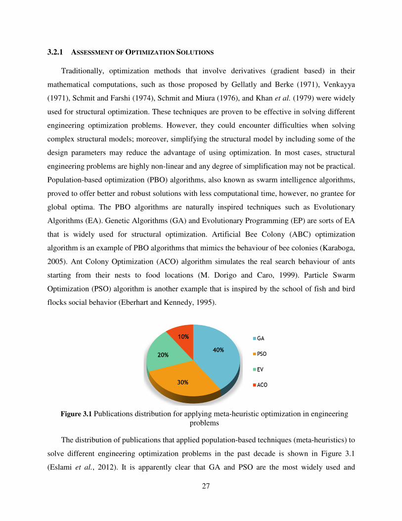
27
3.2.1 ASSESSMENT OF OPTIMIZATION SOLUTIONS
Traditionally, optimization methods that involve derivatives (gradient based) in their
mathematical computations, such as those proposed by Gellatly and Berke (1971), Venkayya
(1971), Schmit and Farshi (1974), Schmit and Miura (1976), and Khan et al. (1979) were widely
used for structural optimization. These techniques are proven to be effective in solving different
engineering optimization problems. However, they could encounter difficulties when solving
complex structural models; moreover, simplifying the structural model by including some of the
design parameters may reduce the advantage of using optimization. In most cases, structural
engineering problems are highly non-linear and any degree of simplification may not be practical.
Population-based optimization (PBO) algorithms, also known as swarm intelligence algorithms,
proved to offer better and robust solutions with less computational time, however, no grantee for
global optima. The PBO algorithms are naturally inspired techniques such as Evolutionary
Algorithms (EA). Genetic Algorithms (GA) and Evolutionary Programming (EP) are sorts of EA
that is widely used for structural optimization. Artificial Bee Colony (ABC) optimization
algorithm is an example of PBO algorithms that mimics the behaviour of bee colonies (Karaboga,
2005). Ant Colony Optimization (ACO) algorithm simulates the real search behaviour of ants
starting from their nests to food locations (M. Dorigo and Caro, 1999). Particle Swarm
Optimization (PSO) algorithm is another example that is inspired by the school of fish and bird
flocks social behavior (Eberhart and Kennedy, 1995).
Figure 3.1 Publications distribution for applying meta-heuristic optimization in engineering
problems
The distribution of publications that applied population-based techniques (meta-heuristics) to
solve different engineering optimization problems in the past decade is shown in Figure 3.1
(Eslami et al., 2012). It is apparently clear that GA and PSO are the most widely used and
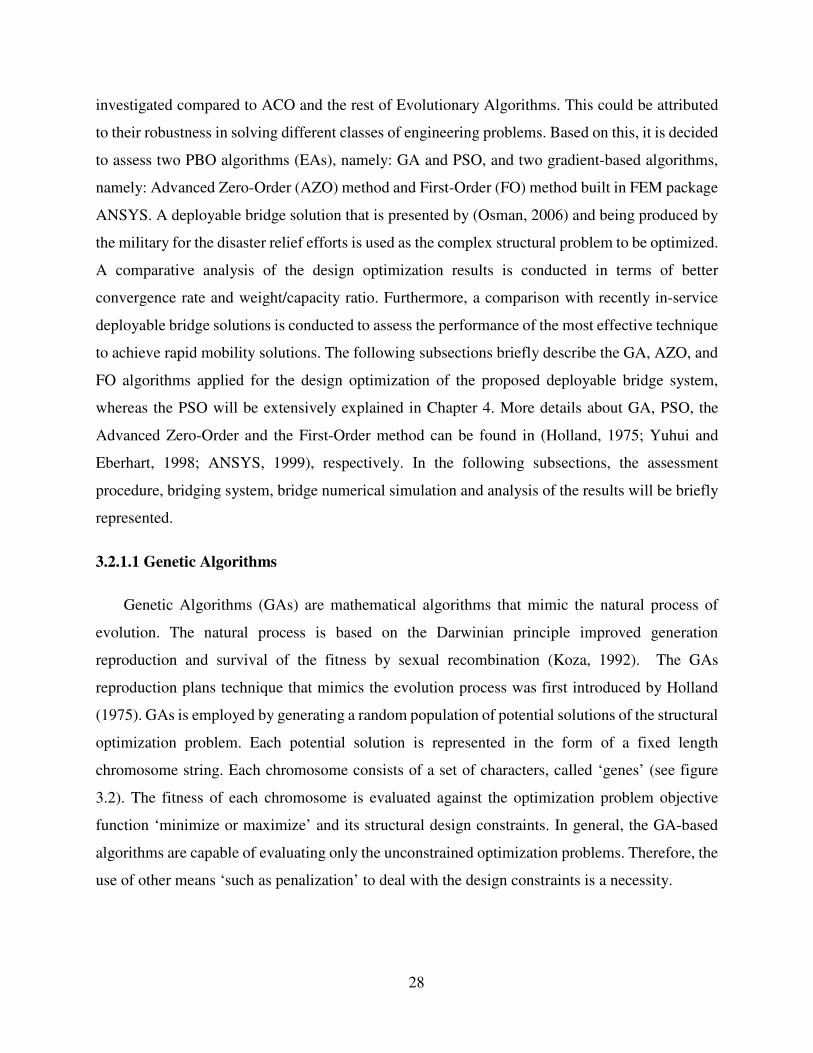
28
investigated compared to ACO and the rest of Evolutionary Algorithms. This could be attributed
to their robustness in solving different classes of engineering problems. Based on this, it is decided
to assess two PBO algorithms (EAs), namely: GA and PSO, and two gradient-based algorithms,
namely: Advanced Zero-Order (AZO) method and First-Order (FO) method built in FEM package
ANSYS. A deployable bridge solution that is presented by (Osman, 2006) and being produced by
the military for the disaster relief efforts is used as the complex structural problem to be optimized.
A comparative analysis of the design optimization results is conducted in terms of better
convergence rate and weight/capacity ratio. Furthermore, a comparison with recently in-service
deployable bridge solutions is conducted to assess the performance of the most effective technique
to achieve rapid mobility solutions. The following subsections briefly describe the GA, AZO, and
FO algorithms applied for the design optimization of the proposed deployable bridge system,
whereas the PSO will be extensively explained in Chapter 4. More details about GA, PSO, the
Advanced Zero-Order and the First-Order method can be found in (Holland, 1975; Yuhui and
Eberhart, 1998; ANSYS, 1999), respectively. In the following subsections, the assessment
procedure, bridging system, bridge numerical simulation and analysis of the results will be briefly
represented.
3.2.1.1 Genetic Algorithms
Genetic Algorithms (GAs) are mathematical algorithms that mimic the natural process of
evolution. The natural process is based on the Darwinian principle improved generation
reproduction and survival of the fitness by sexual recombination (Koza, 1992). The GAs
reproduction plans technique that mimics the evolution process was first introduced by Holland
(1975). GAs is employed by generating a random population of potential solutions of the structural
optimization problem. Each potential solution is represented in the form of a fixed length
chromosome string. Each chromosome consists of a set of characters, called ‘genes’ (see figure
3.2). The fitness of each chromosome is evaluated against the optimization problem objective
function ‘minimize or maximize’ and its structural design constraints. In general, the GA-based
algorithms are capable of evaluating only the unconstrained optimization problems. Therefore, the
use of other means ‘such as penalization’ to deal with the design constraints is a necessity.
29
Figure 3.2 Sexual recombination to generate an offspring through crossover and mutation
Basic GA simulates the survival of fitness by performing three operations, which are
reproduction, crossover, and mutation. The reproduction operation is responsible for the selection
of the best set of chromosomes amongst the generated population to be copied into the new
population. This best set of chromosomes is called, ‘Elite generation’. A chromosome with a
higher fitness has a higher number of offspring based on probability selection criteria’ like roulette
wheel’ (see De Jong, 1975). These best chromosomes exchange their design characteristics to
produce the next offspring through crossover and mutation as clarified in Figure 3.2. The crossover
operation of chromosomes is a commonly biological operation among parents, while mutation is
a scarce operation. Mutation performs a sudden change in the chromosome genes of a randomly
selected offspring, this will allow for a new evolutionary genetic material for next offspring
production and prevent the stagnation around local minima. The new offspring fitness is evaluated
and the process is repeated in order to reach better new generations until a specified criterion is
met. More details about the GA mechanism can be found in (Arora, 2012).
The performance of GA is governed by the selection of four operators, the generation size, the
elite percentage, the crossover probability and the mutation probability, in this study, the GA
operators’ values are chosen as 150, 30, 0.7 and 0.01, respectively. The GA mechanism used is
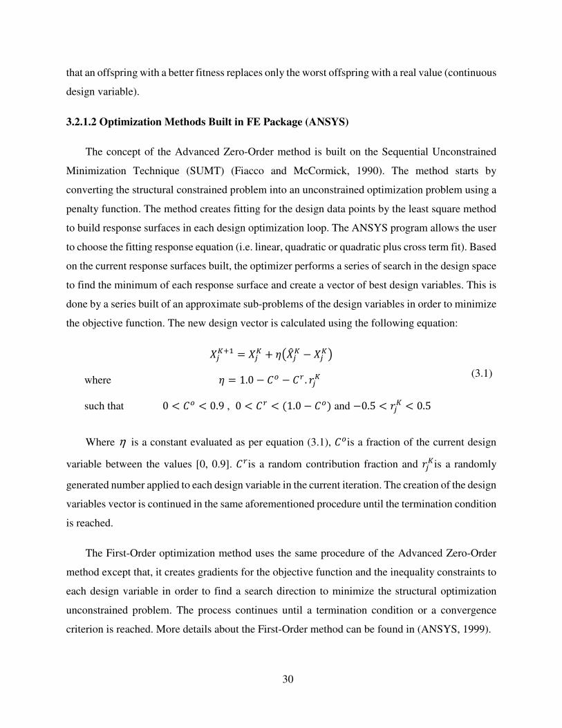
30
that an offspring with a better fitness replaces only the worst offspring with a real value (continuous
design variable).
3.2.1.2 Optimization Methods Built in FE Package (ANSYS)
The concept of the Advanced Zero-Order method is built on the Sequential Unconstrained
Minimization Technique (SUMT) (Fiacco and McCormick, 1990). The method starts by
converting the structural constrained problem into an unconstrained optimization problem using a
penalty function. The method creates fitting for the design data points by the least square method
to build response surfaces in each design optimization loop. The ANSYS program allows the user
to choose the fitting response equation (i.e. linear, quadratic or quadratic plus cross term fit). Based
on the current response surfaces built, the optimizer performs a series of search in the design space
to find the minimum of each response surface and create a vector of best design variables. This is
done by a series built of an approximate sub-problems of the design variables in order to minimize
the objective function. The new design vector is calculated using the following equation:
����� = ��� + ���� − ����
(3.1)
where � = 1.0 − �� − �� . ���
such that 0 < �� < 0.9 , 0 < �� < (1.0 − ��) and −0.5 < ��� < 0.5
Where η is a constant evaluated as per equation (3.1), ��is a fraction of the current design
variable between the values [0, 0.9]. ��is a random contribution fraction and ���is a randomly
generated number applied to each design variable in the current iteration. The creation of the design
variables vector is continued in the same aforementioned procedure until the termination condition
is reached.
The First-Order optimization method uses the same procedure of the Advanced Zero-Order
method except that, it creates gradients for the objective function and the inequality constraints to
each design variable in order to find a search direction to minimize the structural optimization
unconstrained problem. The process continues until a termination condition or a convergence
criterion is reached. More details about the First-Order method can be found in (ANSYS, 1999).
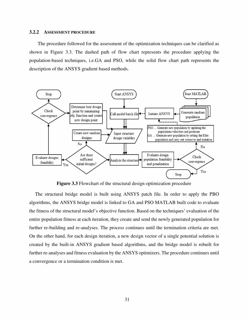
31
3.2.2 ASSESSMENT PROCEDURE
The procedure followed for the assessment of the optimization techniques can be clarified as
shown in Figure 3.3. The dashed path of flow chart represents the procedure applying the
population-based techniques, i.e.GA and PSO, while the solid flow chart path represents the
description of the ANSYS gradient based methods.
The structural bridge model is built using ANSYS patch file. In order to apply the PBO
algorithms, the ANSYS bridge model is linked to GA and PSO MATLAB built code to evaluate
the fitness of the structural model’s objective function. Based on the techniques’ evaluation of the
entire population fitness at each iteration, they create and send the newly generated population for
further re-building and re-analyses. The process continues until the termination criteria are met.
On the other hand, for each design iteration, a new design vector of a single potential solution is
created by the built-in ANSYS gradient based algorithms, and the bridge model is rebuilt for
further re-analyses and fitness evaluation by the ANSYS optimizers. The procedure continues until
a convergence or a termination condition is met.
Figure 3.3 Flowchart of the structural design optimization procedure
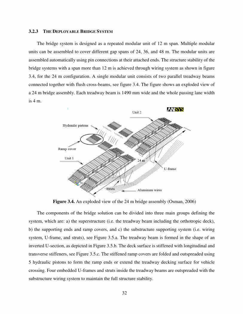
32
3.2.3 THE DEPLOYABLE BRIDGE SYSTEM
The bridge system is designed as a repeated modular unit of 12 m span. Multiple modular
units can be assembled to cover different gap spans of 24, 36, and 48 m. The modular units are
assembled automatically using pin connections at their attached ends. The structure stability of the
bridge systems with a span more than 12 m is achieved through wiring system as shown in figure
3.4, for the 24 m configuration. A single modular unit consists of two parallel treadway beams
connected together with flush cross-beams, see figure 3.4. The figure shows an exploded view of
a 24 m bridge assembly. Each treadway beam is 1490 mm wide and the whole passing lane width
is 4 m.
Figure 3.4. An exploded view of the 24 m bridge assembly (Osman, 2006)
The components of the bridge solution can be divided into three main groups defining the
system, which are: a) the superstructure (i.e. the treadway beam including the orthotropic deck),
b) the supporting ends and ramp covers, and c) the substructure supporting system (i.e. wiring
system, U-frame, and struts), see Figure 3.5.a. The treadway beam is formed in the shape of an
inverted U-section, as depicted in Figure 3.5.b. The deck surface is stiffened with longitudinal and
transverse stiffeners, see Figure 3.5.c. The stiffened ramp covers are folded and outspreaded using
5 hydraulic pistons to form the ramp ends or extend the treadway decking surface for vehicle
crossing. Four embedded U-frames and struts inside the treadway beams are outspreaded with the
substructure wiring system to maintain the full structure stability.
33
Figure 3.5. Tread-way beams cross-section
The Aluminum alloy 7020-T6 material was chosen for manufacturing the bridge system. The
alloy has a density of 2.78 kg/cm3, passion’s ratio of 0.3, modulus of elasticity of 71000 MPa,
yield tensile strength of 280 MPa and an ultimate tensile strength of 350 MPa.
These types of mobile deployable bridge systems are widely functioned in harsh conditions
for the military gap crossing operations and in the aftermath of natural disasters. Therefore, the
guidelines of Trilateral Design and Test Code (TDTC, 2005) which was issued for setting an
internationally accepted design limits for this kind of bridges has been followed. The TDTC
recommends a safety factor of 1.5 of the ultimate tensile strength or 1.33 of the yield tensile
strength for the deployable metallic bridges. The shear strength is taken as 60% of the tensile
allowable. The allowable designs for bending stress and shear stress are chosen as the average
values 224 MPa and 134.4 MPa, respectively. The TDTC code does not impose a serviceability
limit, but a value of 80 mm is taken as a deflection limit to account for any vehicle’s misalignment.
The majority of the existing bridge solutions are capable of supporting a military load capacity
of 60 tons (MLC60) (Kosmatka et al., 2000). This capacity is often unsatisfactory due to the
increasing vehicle design loads. It is noteworthy that a few number of bridge solutions around the
world are capable of supporting a load class of (MLC70) or more; for instance, the BR90 Bridge
system (Winney, 1994), the LEGUAN system (kerr, 1990), and the CAB system (Kosmatka et al.,
U-frame (T10, R3)
Alum. Wires (R2)
H6
W1 (T14, R5)
Strut (T11, R4)
Intermediate stiffener
Cross I-beam
(a) Wiring system design parameters (b) Tread way isometric cross-section
Main stiffener H2 H7
T8
T6 H3 T7
T5
0.745 m
1.25 m
H5
T1
T2
W2
T3 H1
(c) Tread way section design parameters

34
2000). Therefore, the design vehicle load for this bridge is taken as the MLC70 loading class
represented by the hypothetical tracked vehicle MLC70 as required by the TDTC. The tracked
vehicle patch load has a footprint dimension 5000 mm x 900 mm per track. The design loading
conditions are five loading positions for a traveled vehicle: 1) vehicle travel distance is 2000 mm
from support end at the beam center line, 2) 5000 mm centric, 3) 7000 mm centric, 4) 9500 mm
centric, and 5) 9500 mm eccentric. A uniformly distributed load of 76.274 kPa is applied over a
single patch load area. The supporting conditions of the bridge are set as a simple supported.
3.2.3.1 Numerical Simulation
The FEM of the mobile deployable bridge is numerically simulated using the ANSYS
Parametric Design Language (APDL). A set of thirty design parameters are chosen to define the
mobile bridge’s different components and are classified into three groups as follows: 1) the
treadway beams’ deign parameters, 2) the bridge end supports and ramp covers’ design parameters,
and 3) the substructure design parameters (i.e. U-frames, struts, compression posts and the wiring
system).
The description of the aforementioned thirty design parameters is tabulated in Table 3.1 and
they are demonstrated in Figures 3.5.a and 3.5.c. All the treadway plate elements are modeled
using Shell181 element. The U-frame and beam struts are modeled using Beam188 element. The
aluminum wires, accounting for tension only, are modeled using Link181 element whereas the
hydraulic pistons are modeled as compression posts (i.e. no damping is considered) using Link11
element. A subroutine program is developed to create up to 10 automatic meshing trials per single
design analysis in order to improve the meshing quality. The average number of elements created
for one design analysis is 65200 elements.
3.2.3.2 Numerical Evaluation
The formulation of the optimization problem for the case of minimizing the bridge structural
weight �(�) under an imposed strength and deflection constraints �(�) can be as follows:
35
Minimize: ( ) ( ) ( )∑=
=
elem
elem
1den
n
i
ii xLxAxF ρ
Subjected to: ( )
1~ ,
,≤
Stri
lStrri
G
xG,r=1,2,…,nload,� = 1,2, … , !elem, % = &1, &2or&3
( )
1~ ef
, ≤D
Defrm
G
xG, r=1,2,…,nload,* = 1,2, … , !node
Uj
ij
Lj xxx ≤≤ and 1,2,...,30 =j
(3.2)
where -./01213 is the alloy material density, 45(�) is the discretized FEM cross-sectional area.
65(�) is the discretized element length. �5,�78�,�(�) and �9578�are the calculated and the allowable
stress constraints, respectively. �:,�;<=(�) and �9;<=are the calculated and the allowable deflection
constraints, respectively. The symbols r and l are the loading conditions and the principal stresses’
indices, respectively. ��> and ��? are the lower and upper bounds of the plate thickness ��5 assigned
to the cross-sectional area numbered i, respectively.
The gradient-based techniques start the optimization analysis from a single feasible initial
solution. A random search is created to probe several feasible solutions in the design space. In
order to enhance the performance of the Advanced Zero-Order method and the First-Order method
optimization processes, five independent iterations are conducted for each method starting from a
different initial feasible solution obtained by the random search. The random search started from
an initial conventional design of 13.099 tons and the design parameters' values are illustrated in
Table 3.1; From 200 random iterations, only 31 feasible design are obtained. The values of the
best five feasible designs obtained by the random search in descending order are 11.785, 11.599,
11.287, 11.181 and 10.974 tons.
After applying the Zero-Order optimization’s five trials, the best weight results obtained by
the method are 9.349, 10.312, 9.904, 10.367, and 10.461 tons. The design parameters’ values for
the best result (9.349 tons) are illustrated in Table 3.1. It can be clearly seen that starting from a
minimum initial feasible design is not a guarantee to obtain the optimal result (i.e. 10.974 tons
initial design results in 10.461 tons optimized design). The method succeeded in reducing the
weight of the deployable bridge by 28.6%.
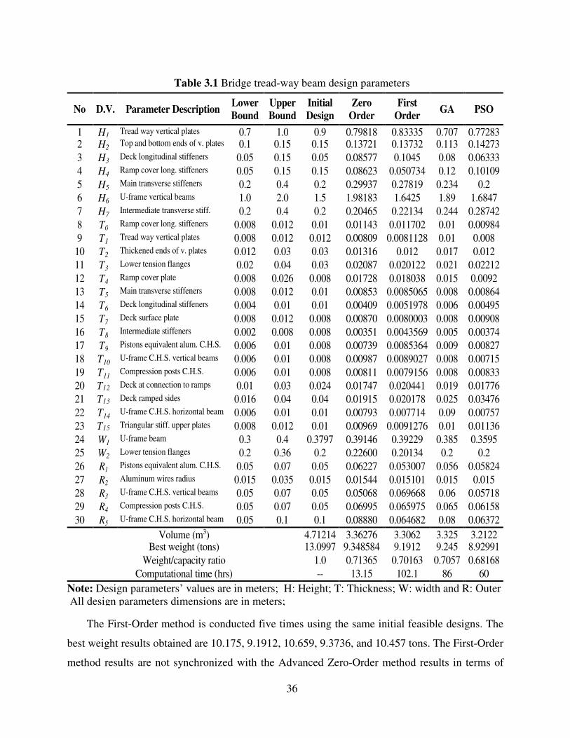
36
The First-Order method is conducted five times using the same initial feasible designs. The
best weight results obtained are 10.175, 9.1912, 10.659, 9.3736, and 10.457 tons. The First-Order
method results are not synchronized with the Advanced Zero-Order method results in terms of
Table 3.1 Bridge tread-way beam design parameters
No D.V. Parameter Description Lower
Bound
Upper
Bound
Initial
Design
Zero
Order
First
Order GA PSO
1 H1 Tread way vertical plates 0.7 1.0 0.9 0.79818 0.83335 0.707 0.77283 2 H2 Top and bottom ends of v. plates 0.1 0.15 0.15 0.13721 0.13732 0.113 0.14273 3 H3 Deck longitudinal stiffeners 0.05 0.15 0.05 0.08577 0.1045 0.08 0.06333 4 H4 Ramp cover long. stiffeners 0.05 0.15 0.15 0.08623 0.050734 0.12 0.10109 5 H5 Main transverse stiffeners 0.2 0.4 0.2 0.29937 0.27819 0.234 0.2 6 H6 U-frame vertical beams 1.0 2.0 1.5 1.98183 1.6425 1.89 1.6847 7 H7 Intermediate transverse stiff. 0.2 0.4 0.2 0.20465 0.22134 0.244 0.28742 8 T0 Ramp cover long. stiffeners 0.008 0.012 0.01 0.01143 0.011702 0.01 0.00984 9 T1 Tread way vertical plates 0.008 0.012 0.012 0.00809 0.0081128 0.01 0.008 10 T2 Thickened ends of v. plates 0.012 0.03 0.03 0.01316 0.012 0.017 0.012 11 T3 Lower tension flanges 0.02 0.04 0.03 0.02087 0.020122 0.021 0.02212 12 T4 Ramp cover plate 0.008 0.026 0.008 0.01728 0.018038 0.015 0.0092 13 T5 Main transverse stiffeners 0.008 0.012 0.01 0.00853 0.0085065 0.008 0.00864 14 T6 Deck longitudinal stiffeners 0.004 0.01 0.01 0.00409 0.0051978 0.006 0.00495 15 T7 Deck surface plate 0.008 0.012 0.008 0.00870 0.0080003 0.008 0.00908 16 T8 Intermediate stiffeners 0.002 0.008 0.008 0.00351 0.0043569 0.005 0.00374 17 T9 Pistons equivalent alum. C.H.S. 0.006 0.01 0.008 0.00739 0.0085364 0.009 0.00827 18 T10 U-frame C.H.S. vertical beams 0.006 0.01 0.008 0.00987 0.0089027 0.008 0.00715 19 T11 Compression posts C.H.S. 0.006 0.01 0.008 0.00811 0.0079156 0.008 0.00833 20 T12 Deck at connection to ramps 0.01 0.03 0.024 0.01747 0.020441 0.019 0.01776 21 T13 Deck ramped sides 0.016 0.04 0.04 0.01915 0.020178 0.025 0.03476 22 T14 U-frame C.H.S. horizontal beam 0.006 0.01 0.01 0.00793 0.007714 0.09 0.00757 23 T15 Triangular stiff. upper plates 0.008 0.012 0.01 0.00969 0.0091276 0.01 0.01136 24 W1 U-frame beam 0.3 0.4 0.3797 0.39146 0.39229 0.385 0.3595 25 W2 Lower tension flanges 0.2 0.36 0.2 0.22600 0.20134 0.2 0.2 26 R1 Pistons equivalent alum. C.H.S. 0.05 0.07 0.05 0.06227 0.053007 0.056 0.05824 27 R2 Aluminum wires radius 0.015 0.035 0.015 0.01544 0.015101 0.015 0.015 28 R3 U-frame C.H.S. vertical beams 0.05 0.07 0.05 0.05068 0.069668 0.06 0.05718 29 R4 Compression posts C.H.S. 0.05 0.07 0.05 0.06995 0.065975 0.065 0.06158 30 R5 U-frame C.H.S. horizontal beam 0.05 0.1 0.1 0.08880 0.064682 0.08 0.06372
Volume (m3) 4.71214 3.36276 3.3062 3.325 3.2122 Best weight (tons) 13.0997 9.348584 9.1912 9.245 8.92991
Weight/capacity ratio 1.0 0.71365 0.70163 0.7057 0.68168 Computational time (hrs) -- 13.15 102.1 86 60
Note: Design parameters’ values are in meters; H: Height; T: Thickness; W: width and R: Outer All design parameters dimensions are in meters;
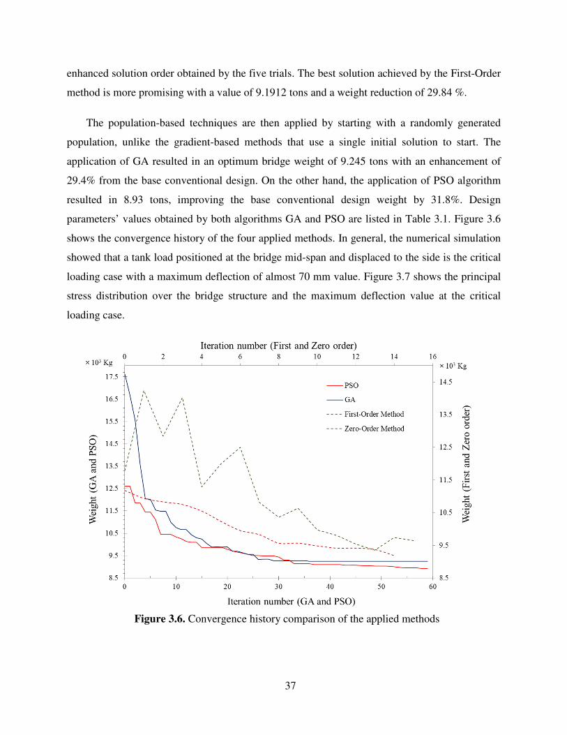
37
enhanced solution order obtained by the five trials. The best solution achieved by the First-Order
method is more promising with a value of 9.1912 tons and a weight reduction of 29.84 %.
The population-based techniques are then applied by starting with a randomly generated
population, unlike the gradient-based methods that use a single initial solution to start. The
application of GA resulted in an optimum bridge weight of 9.245 tons with an enhancement of
29.4% from the base conventional design. On the other hand, the application of PSO algorithm
resulted in 8.93 tons, improving the base conventional design weight by 31.8%. Design
parameters’ values obtained by both algorithms GA and PSO are listed in Table 3.1. Figure 3.6
shows the convergence history of the four applied methods. In general, the numerical simulation
showed that a tank load positioned at the bridge mid-span and displaced to the side is the critical
loading case with a maximum deflection of almost 70 mm value. Figure 3.7 shows the principal
stress distribution over the bridge structure and the maximum deflection value at the critical
loading case.
Figure 3.6. Convergence history comparison of the applied methods
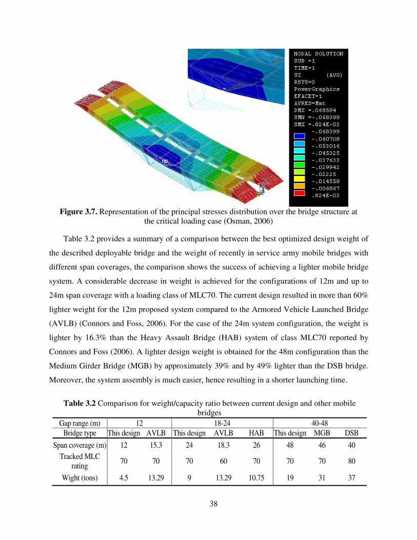
38
Figure 3.7. Representation of the principal stresses distribution over the bridge structure at
the critical loading case (Osman, 2006)
Table 3.2 provides a summary of a comparison between the best optimized design weight of
the described deployable bridge and the weight of recently in service army mobile bridges with
different span coverages, the comparison shows the success of achieving a lighter mobile bridge
system. A considerable decrease in weight is achieved for the configurations of 12m and up to
24m span coverage with a loading class of MLC70. The current design resulted in more than 60%
lighter weight for the 12m proposed system compared to the Armored Vehicle Launched Bridge
(AVLB) (Connors and Foss, 2006). For the case of the 24m system configuration, the weight is
lighter by 16.3% than the Heavy Assault Bridge (HAB) system of class MLC70 reported by
Connors and Foss (2006). A lighter design weight is obtained for the 48m configuration than the
Medium Girder Bridge (MGB) by approximately 39% and by 49% lighter than the DSB bridge.
Moreover, the system assembly is much easier, hence resulting in a shorter launching time.
Table 3.2 Comparison for weight/capacity ratio between current design and other mobile bridges
Gap range (m) 12 18-24 40-48 Bridge type This design AVLB This design AVLB HAB This design MGB DSB
Span coverage (m) 12 15.3 24 18.3 26 48 46 40 Tracked MLC
rating 70 70 70 60 70 70 70 80
Wight (tons) 4.5 13.29 9 13.29 10.75 19 31 37
39
Based on the conducted analysis of results, it is found that PSO performs better for optimizing
this type of complex bridge structural systems in terms of convergence rate and best solution, while
being second best in terms of computational time. Generally, a promising achievement is found
for the application of structural design optimization to reach an effective deployable bridge system
for post-disaster rapid mobility through a comparison with recently in service mobile bridges.
Therefore, the PSO algorithm is chosen for the composite deployable bridge optimization in this
research study.
3.3 SUMMARY
In this chapter, four optimization algorithms from Meta-heuristics (i.e. GA and PSO) and
gradient-based techniques (i.e. Zero-order and First-order) are applied for their performance
assessment on a deployable bridge structure. The deployable bridge structure is simulated using
the direct generation method in ANSYS finite element package. The four optimization algorithms’
mechanism are briefly described and coded in MATLAB then integrated with the FE software.
Based on the conducted performance assessment, PSO proved to perform better for this kind of
bridge structures. Therefore, the PSO algorithm is chosen for further investigation and
improvement to suit complex structural problems.
In the following chapter, a representation is illustrated of the candidate algorithm’s mechanism,
advantages, disadvantages and the modifications developed to minimize, up to a considerable
limit, PSO deficiencies in order to adapt an effective structural design optimization of large-scale
and complex structures.
40
CHAPTER 4
Controlled-Diversity Swarm
Optimization
4.1 INTRODUCTION
PSO outperforms other PBO algorithms in many aspects based on a comprehensive literature
review and the investigation presented in Chapter 3. However, similar to other PBO algorithms,
PSO suffers from a premature convergence after few iterations that may result in falling in local
minima. This deficiency may affect to a considerable limit the optimization efficiency for complex
structural models. Therefore, this chapter aims to present new modifications to PSO in order to
enhance the algorithm performance and minimize its deficiency to structural design optimization.
The proposed algorithm, Controlled Diversity Particle Swarm Optimizer (CD-PSO), is based on
the attraction and repulsion phenomenon of the flock of birds, such that a better balance between
exploration and exploitation could be achieved. Further, the modified swarm intelligence optimizer
is hybridized with Response Surface Methodology (RSM) as a tool to distinguish the influence
level of design parameters to the objective function in complex structural models. Based on a
specific criterion, hybrid PSO enhances the swarm search in order to seek for better solutions. CD-
PSO performance is evaluated through tests on three benchmark truss structures for the minimum
weight design. Finally, the performance of hybrid CD-PSO and its integration with RSM along
with original CD-PSO is examined for weight minimization of the deployable bridge model
presented in the previous chapter.
4.2 PARTICLE SWARM OPTIMIZATION ALGORITHM
Particle Swarm Optimization (PSO) is an intelligence search technique that is stochastic in
nature. First proposed by Eberhart & Kennedy (1995), the PSO algorithm directs the search to the
nearest optima simulating the swarm social behavior. The swarm population consists of Np mass-
less and volume-less particles, where each particle represents a potential solution of the problem.
4

41
The algorithm randomly initiates and distributes the particles to probe the promising feasible
regions in hyperspace. These particles, forming the swarm cloud, move with changing velocities
and share their successful information with other particles while exploring the multi-dimensional
hyperspace. Each particle updates its velocity and position based on its own best experience and
best experience gained by the whole swarm. Each particle, i, in the swarm, encodes a number of
design parameters, n. The particle is represented by a position vector Xij=Ax1i , �2
i , …�ni B that is
updated using the velocity vector Vij=Av1i , v2
i , …vni B. The equations of the particle’s updated
velocity and position vectors were given by Yuhui and Eberhart (1998).
( ) ( ) - - . ),(),(22
),(),(11
),()1,( Kij
KijG
Kij
KijP
Kij
Kij XXrcXXrcVwV ⋅⋅+⋅⋅+=+ (4.1)
)1,(),()1,( ++ += Kij
Kij
Kij VXX (4.2)
where ��(5,�)and C�(5,�)are the current position and velocity of the ith particle in the jth dimension
of hyperspace, respectively. The parameter K is the time interval of search history, ��(5,�)D
represents the best experience by the particle which is conceptually resembling an
autobiographical memory, and ��(5,�)E is the best experience gained by the entire swarm. F� and
FG are the cognition and social parameters, respectively, and they were defined by Eberhart and
Kennedy (1995) as acceleration factors. The acceleration factors weigh the velocity of each
particle to its previous local best or to the global best at the Kth iteration (i.e. a higher value of F� contributes more to local best and higher value of FG contributes more to a global best). Generally,
the acceleration factors are within the range of [0, 4]. r1 and r2 are any randomly selected real
numbers in the interval of [0, 1]. The updated velocity Equation 4.1 consists of the summation of
three terms; the weighted velocity for exploration, the self-cognition learning, and the social
learning. In order to balance between exploration and exploitation, the impact of the previous
velocities on the current particle velocity C�(5,�) is weighted by the inertia factor w . Through the
entire search history, a large inertia weight is applied at initial travel stages to enable a global
exploration of the hyperspace. When the swarm search gets closer to the optimum domain, a small
inertia weight is recommended for exploitation. A linear decrease of inertia weight can be achieved
using the equation given by Eberhart and Yuhui (2001).
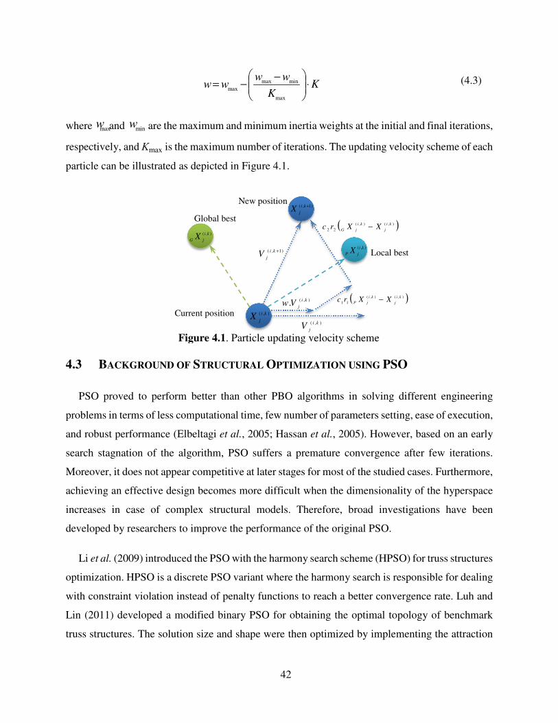
42
Global best
),( ki
jPX
),( ki
jGX
),( ki
jX
)1,( +ki
jX
),( ki
jV
),(. ki
jVw ( )),(),(
11
ki
j
ki
jPXXrc −
)1,( +ki
jV
( )),(),(22
ki
j
ki
jGXXrc −
Local best
Current position
New position
KK
wwww ⋅
−−=
max
minmaxmax
(4.3)
where maxw and minw are the maximum and minimum inertia weights at the initial and final iterations,
respectively, and Kmax is the maximum number of iterations. The updating velocity scheme of each
particle can be illustrated as depicted in Figure 4.1.
Figure 4.1. Particle updating velocity scheme
4.3 BACKGROUND OF STRUCTURAL OPTIMIZATION USING PSO
PSO proved to perform better than other PBO algorithms in solving different engineering
problems in terms of less computational time, few number of parameters setting, ease of execution,
and robust performance (Elbeltagi et al., 2005; Hassan et al., 2005). However, based on an early
search stagnation of the algorithm, PSO suffers a premature convergence after few iterations.
Moreover, it does not appear competitive at later stages for most of the studied cases. Furthermore,
achieving an effective design becomes more difficult when the dimensionality of the hyperspace
increases in case of complex structural models. Therefore, broad investigations have been
developed by researchers to improve the performance of the original PSO.
Li et al. (2009) introduced the PSO with the harmony search scheme (HPSO) for truss structures
optimization. HPSO is a discrete PSO variant where the harmony search is responsible for dealing
with constraint violation instead of penalty functions to reach a better convergence rate. Luh and
Lin (2011) developed a modified binary PSO for obtaining the optimal topology of benchmark
truss structures. The solution size and shape were then optimized by implementing the attraction
43
and repulsion of swarm particles (ARPSO) in order to improve the solution quality. Kaveh (2014)
proposed the Chaotic Swarming of Particles (CSP) algorithm, in which the particles use the
random chaotic search theory to escape from local minima and reach a robust solution. Other
research efforts were done earlier by Fourie and Groenwold (2002), Schutte and Groenwold
(2003), Perez and Behdinan (2007), and Luh and Lin (2008). Generally, research efforts for
developing PSO variants can be classified into four categories based on; parameter tuning,
neighborhood topology, learning strategies and hybridization. Learning strategies and
hybridization research based algorithms showed the promising convergence results closer to the
optimum solution amongst the four categories (Tanweer et al., 2015).
The current study presents a new PSO algorithm that is based on a technique for controlling the
attraction and repulsion phenomenon of the swarm. Earlier studies that emulated the flock
attraction and repulsion were not effective for structural design optimization after been tested. A
control criterion is applied to the proposed algorithm CD-PSO to prevent the swarm’s diversity
stagnation and to achieve an effective balance between exploration and exploitation. The diversity
control technique is presented in which the swarm diversity is regulated using a nonlinear
decreasing repulsion surface. The repulsion surface forces the swarm to oscillate between
attraction and repulsion in a decaying manner. The controlling technique along with other earlier
versions emulated this swarm behavior are comprehensively described in Section 4.4
The concept of CD-PSO is evaluated through a comparison with the classical PSO as well as
other four algorithms and the evaluation of the results is presented in Section 4.5; three of them
are based on learning strategies (earlier versions of attraction and repulsion) whereas the fourth
one is based on hybridization. Moreover, a comparative statistical analysis between the proposed
CD-PSO and other algorithms in the literature is conducted. Three benchmark truss structures are
selected to validate the effectiveness of the proposed algorithm and the diversity control technique.
The results are analyzed and compared in terms of computational time, algorithm stability and
solution quality. Finally, in order to achieve better assessment and further enhancement of CD-
PSO to optimize large-scale and complex structural models, a hybridized CD-PSO with RSM and
original CD-PSO performances are examined on the deployable bridge system proposed in the
previous chapter. Original CD-PSO is applied two times, first while considering all the design
parameters of the bridge model. The second is applied while considering only the effective design
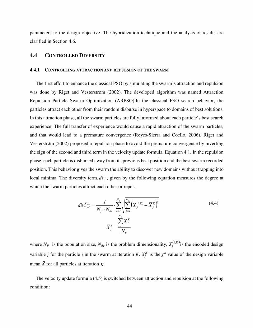
44
parameters to the design objective. The hybridization technique and the analysis of results are
clarified in Section 4.6.
4.4 CONTROLLED DIVERSITY
4.4.1 CONTROLLING ATTRACTION AND REPULSION OF THE SWARM
The first effort to enhance the classical PSO by simulating the swarm`s attraction and repulsion
was done by Riget and Vesterstrøm (2002). The developed algorithm was named Attraction
Repulsion Particle Swarm Optimization (ARPSO).In the classical PSO search behavior, the
particles attract each other from their random disburse in hyperspace to domains of best solutions.
In this attraction phase, all the swarm particles are fully informed about each particle`s best search
experience. The full transfer of experience would cause a rapid attraction of the swarm particles,
and that would lead to a premature convergence (Reyes-Sierra and Coello, 2006). Riget and
Vesterstrøm (2002) proposed a repulsion phase to avoid the premature convergence by inverting
the sign of the second and third term in the velocity update formula, Equation 4.1. In the repulsion
phase, each particle is disbursed away from its previous best position and the best swarm recorded
position. This behavior gives the swarm the ability to discover new domains without trapping into
local minima. The diversity term, div , given by the following equation measures the degree at
which the swarm particles attract each other or repel.
( )( )∑ ∑= =
= −⋅⋅
=p dv
N
1i
N
1j
2K
j
Ki
j
dvp
K
0itr XXNN
1 div
,max (4.4)
p
N
1i
K
jK
jN
X
X
p
∑==
where NP is the population size, Ndv is the problem dimensionality, ��(5,�)is the encoded design
variable j for the particle i in the swarm at iteration K. �I�� is the jth value of the design variable
mean �I for all particles at iteration K.
The velocity update formula (4.5) is switched between attraction and repulsion at the following
condition:
45
( )( ) ( )( ) - - . ),(),(222
),(),(111
),()1,( Ki
j
Ki
jG
Ki
j
Ki
jP
Ki
j
Ki
jXXrcdirXXrcdirVwV ⋅⋅⋅+⋅⋅⋅+=+ (4.5)
Such that:
<−
≥+==
low
high
ddiv
ddivdirdir
if 1
if 121
When particles attract each other, the diversity decreases until it reaches a lower limit, dlow,
equals to 5.0 × 10⁻⁶. Consequently, the swarm cloud is switched to the repulsion phase. As a result,
the swarm cloud expands and the diversity increases until it reaches an upper limit, dhigh, equals to
0.25. At this stage, the swarm cloud returns back to attraction again (Riget and Vesterstrøm, 2002).
Pantetal et al. (2007) proposed the Attraction Repulsion PSO (ATRE-PSO) which is another
version of ARPSO. For this algorithm, in addition to the attraction and repulsion phases, a third
phase is considered and identified as the positive conflict phase. In this phase, neither full attraction
nor repulsion would occur if the swarm cloud diversity lies between the values of dlow and dhigh. In
this case, the velocity update condition is modified as follows:
<−=−=
≤≤−=+=
>+=+=
low
highlow
high
ddivdirdir
ddivddirdir
ddivdirdir
if 1 ,1
if 1 ,1
if 1 ,1
21
21
21
Li and Li (2012) proposed the Diversity Guided PSO (DGPSO) in which they added two phases
to the ARPSO between full attraction and full repulsion to keep a high swarm diversity. The whole
swarm cloud will be shuttling between these phases under the following conditions:
( )( )
<−=−=
+≤≤−=+=
≤<++=−=
>+=+=
low21
highlowlow21
highhighlow21
high21
ddiv if 1 dir 1dir
2dddivd if 1 dir 1dir
ddiv2dd if 1 dir 1dir
ddiv if 1 dir 1dir
,
/,
/,
,
The three aforementioned studies specified two fixed values for dlow and dhigh to switch between
phases. These values give promising results when tested over benchmark functions, however, they
are unable to assure a promising diversity control of the swarm for structural engineering problems
even if they are tuned. In structural engineering problems, the initial population of the swarm is
usually smaller than that of benchmark functions to adopt the problem complexities and reduce
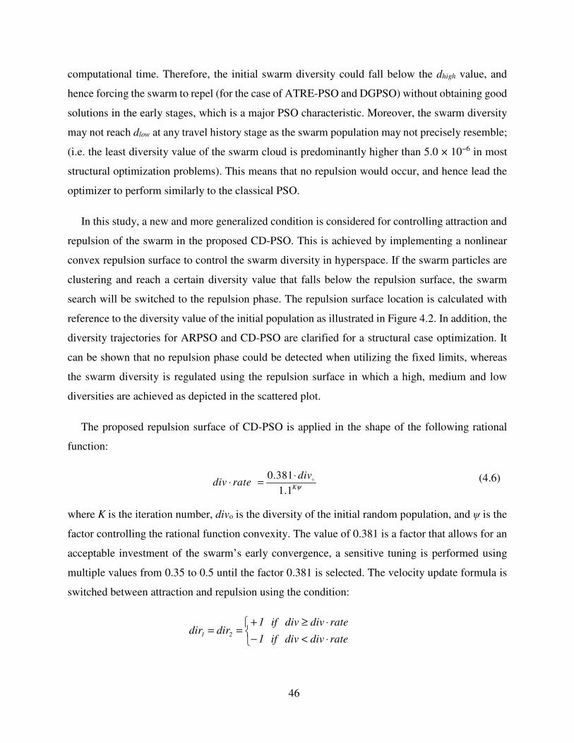
46
computational time. Therefore, the initial swarm diversity could fall below the dhigh value, and
hence forcing the swarm to repel (for the case of ATRE-PSO and DGPSO) without obtaining good
solutions in the early stages, which is a major PSO characteristic. Moreover, the swarm diversity
may not reach dlow at any travel history stage as the swarm population may not precisely resemble;
(i.e. the least diversity value of the swarm cloud is predominantly higher than 5.0 × 10⁻⁶ in most
structural optimization problems). This means that no repulsion would occur, and hence lead the
optimizer to perform similarly to the classical PSO.
In this study, a new and more generalized condition is considered for controlling attraction and
repulsion of the swarm in the proposed CD-PSO. This is achieved by implementing a nonlinear
convex repulsion surface to control the swarm diversity in hyperspace. If the swarm particles are
clustering and reach a certain diversity value that falls below the repulsion surface, the swarm
search will be switched to the repulsion phase. The repulsion surface location is calculated with
reference to the diversity value of the initial population as illustrated in Figure 4.2. In addition, the
diversity trajectories for ARPSO and CD-PSO are clarified for a structural case optimization. It
can be shown that no repulsion phase could be detected when utilizing the fixed limits, whereas
the swarm diversity is regulated using the repulsion surface in which a high, medium and low
diversities are achieved as depicted in the scattered plot.
The proposed repulsion surface of CD-PSO is applied in the shape of the following rational
function:
0.381
1.1K
divdiv rate
ψ
⋅⋅ = o (4.6)
where K is the iteration number, divo is the diversity of the initial random population, and ψ is the
factor controlling the rational function convexity. The value of 0.381 is a factor that allows for an
acceptable investment of the swarm’s early convergence, a sensitive tuning is performed using
multiple values from 0.35 to 0.5 until the factor 0.381 is selected. The velocity update formula is
switched between attraction and repulsion using the condition:
⋅<−
⋅≥+==
ratedivdiv if 1
ratedivdiv if 1dirdir 21
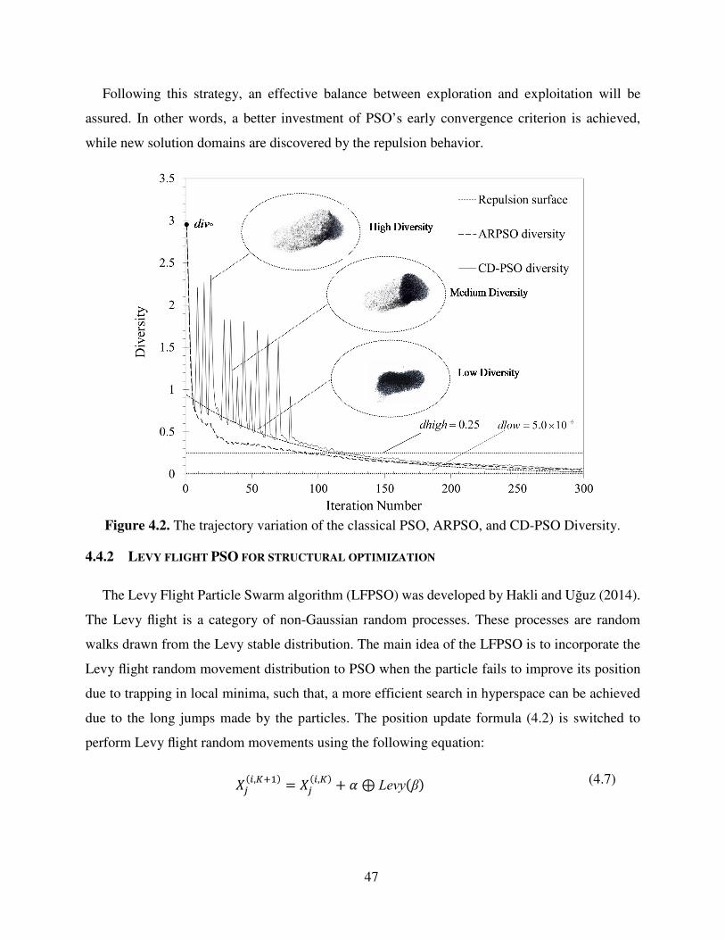
47
Following this strategy, an effective balance between exploration and exploitation will be
assured. In other words, a better investment of PSO’s early convergence criterion is achieved,
while new solution domains are discovered by the repulsion behavior.
Figure 4.2. The trajectory variation of the classical PSO, ARPSO, and CD-PSO Diversity.
4.4.2 LEVY FLIGHT PSO FOR STRUCTURAL OPTIMIZATION
The Levy Flight Particle Swarm algorithm (LFPSO) was developed by Hakli and Uğuz (2014).
The Levy flight is a category of non-Gaussian random processes. These processes are random
walks drawn from the Levy stable distribution. The main idea of the LFPSO is to incorporate the
Levy flight random movement distribution to PSO when the particle fails to improve its position
due to trapping in local minima, such that, a more efficient search in hyperspace can be achieved
due to the long jumps made by the particles. The position update formula (4.2) is switched to
perform Levy flight random movements using the following equation:
��(5,���� � ���5,��
� J ⊕ Levy(β) (4.7)

48
where α is the skewness parameter of the levy distribution which is chosen as a random number,
and β is the Levy index that controls the shapes of the probability distribution, such that, smaller
β values perform longer particles jumps, hence elongated distribution tails. The product ⊕ means
an element-wise multiplication. A more comprehensive explanation of the Levy flight motion is
demonstrated by Chechkin et al. (2008). LFPSO proved to provide a high diversity distribution to
avoid particlesꞌ trapping in local minima when it is applied to benchmark functions. In this study,
the hybrid LFPSO was reformulated to suit the structural optimization for a comparative statistical
analysis with the proposed CD-PSO.
4.5 ASSESSMENT OF CD-PSO ON BENCHMARK STRUCTURES
The effectiveness of the proposed CD-PSO algorithm on structural optimization is assessed
through tests on three benchmark truss structures: A 10-member planar truss, a 25-member spatial
truss, and a 72-member spatial truss. For the 10, 25 and 72-member structural benchmark
problems, the swarm population is chosen as 100, 40 and 40, and the maximum number of
iterations is set to 2000, 250 and 200, respectively. Table 4.1 illustrates the CD-PSO operators’
values used for running the three optimization tests. The following subsections present a
comparison between the numerical results of the proposed CD-PSO algorithm and the results data
in the literature.
Table 4.1 Optimization operators of CD-PSO and the rational function convexity factors
Truss benchmark optimization parameters Operator value
Acceleration factors c1 and c2 2.0, 2.0 Maximum inertia weight wmax 0.9
Minimum inertia weight wmin 0.4 Velocity bounds Vmax and Vmin +10%, -10%
Rational function convexity factor ψ 0.125 and 0.15
4.5.1 PROBLEMS FORMULATION AND FEASIBILITY MANAGEMENT
In general, the optimization problem formulation for the minimum weight �(�) design of the
benchmark truss structures under an imposed strength and deflection constraints �(�) can be
expressed in a standard formulation as follows:
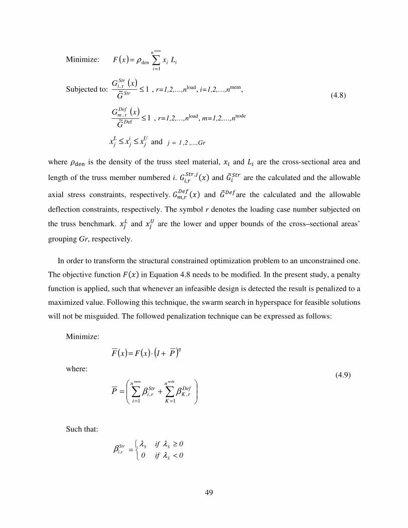
49
Minimize: ( ) ∑=
=
mem
1den
n
i
ii L xxF ρ
Subjected to: ( )
1~ r ,
≤Str
Stri
G
xG , r=1,2,…,nload,i=1,2,…,nmem,
( )
1~ ef
r , ≤
D
Defm
G
xG , r=1,2,…,nload,m=1,2,…,nnode
and ,...,Gr2,1j =
(4.8)
where -./0 is the density of the truss steel material, �5 and 65 are the cross-sectional area and
length of the truss member numbered i. �5,�78�,�(�) and �9578� are the calculated and the allowable
axial stress constraints, respectively.�:,�;<=(�) and �9;<=are the calculated and the allowable
deflection constraints, respectively. The symbol r denotes the loading case number subjected on
the truss benchmark. ��> and ��? are the lower and upper bounds of the cross–sectional areas’
grouping Gr, respectively.
In order to transform the structural constrained optimization problem to an unconstrained one.
The objective function �(�)in Equation 4.8 needs to be modified. In the present study, a penalty
function is applied, such that whenever an infeasible design is detected the result is penalized to a
maximized value. Following this technique, the swarm search in hyperspace for feasible solutions
will not be misguided. The followed penalization technique can be expressed as follows:
Minimize:
( ) ( ) ( )ηP 1 xF xF +⋅=
where:
+= ∑ ∑
= =
mem node
1 1,,
n
i
n
K
DefrK
StrriP ββ
(4.9)
Such that:
Str
ri,β
<
≥=
0 if0
0 if
S
SS
λ
λλ
Uj
ij
Lj xxx ≤≤
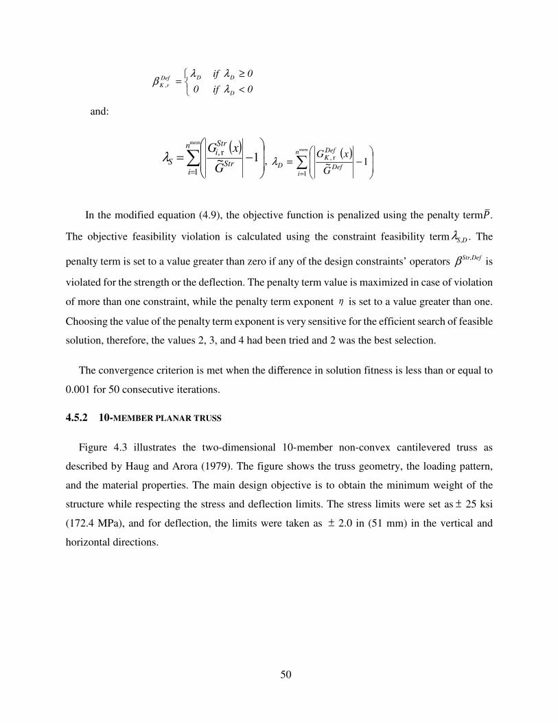
50
<
≥=
0 if0
0 if
D
DDDef
rKλ
λλβ ,
and:
( )
∑=
−=
mem
1
r , 1~ n
iStr
Stri
SG
xGλ ,
( )∑
=
−=
mem
1
r , 1~ n
iDef
DefK
DG
xGλ
In the modified equation (4.9), the objective function is penalized using the penalty termMI. The objective feasibility violation is calculated using the constraint feasibility term DS,λ . The
penalty term is set to a value greater than zero if any of the design constraints’ operators DefStr,β is
violated for the strength or the deflection. The penalty term value is maximized in case of violation
of more than one constraint, while the penalty term exponent η is set to a value greater than one.
Choosing the value of the penalty term exponent is very sensitive for the efficient search of feasible
solution, therefore, the values 2, 3, and 4 had been tried and 2 was the best selection.
The convergence criterion is met when the difference in solution fitness is less than or equal to
0.001 for 50 consecutive iterations.
4.5.2 10-MEMBER PLANAR TRUSS
Figure 4.3 illustrates the two-dimensional 10-member non-convex cantilevered truss as
described by Haug and Arora (1979). The figure shows the truss geometry, the loading pattern,
and the material properties. The main design objective is to obtain the minimum weight of the
structure while respecting the stress and deflection limits. The stress limits were set as ± 25 ksi
(172.4 MPa), and for deflection, the limits were taken as ± 2.0 in (51 mm) in the vertical and
horizontal directions.
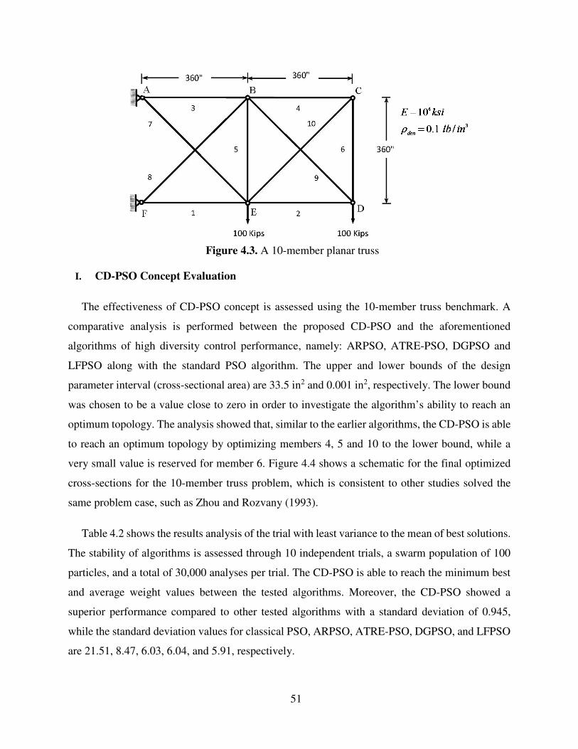
51
Figure 4.3. A 10-member planar truss
I. CD-PSO Concept Evaluation
The effectiveness of CD-PSO concept is assessed using the 10-member truss benchmark. A
comparative analysis is performed between the proposed CD-PSO and the aforementioned
algorithms of high diversity control performance, namely: ARPSO, ATRE-PSO, DGPSO and
LFPSO along with the standard PSO algorithm. The upper and lower bounds of the design
parameter interval (cross-sectional area) are 33.5 in2 and 0.001 in2, respectively. The lower bound
was chosen to be a value close to zero in order to investigate the algorithm’s ability to reach an
optimum topology. The analysis showed that, similar to the earlier algorithms, the CD-PSO is able
to reach an optimum topology by optimizing members 4, 5 and 10 to the lower bound, while a
very small value is reserved for member 6. Figure 4.4 shows a schematic for the final optimized
cross-sections for the 10-member truss problem, which is consistent to other studies solved the
same problem case, such as Zhou and Rozvany (1993).
Table 4.2 shows the results analysis of the trial with least variance to the mean of best solutions.
The stability of algorithms is assessed through 10 independent trials, a swarm population of 100
particles, and a total of 30,000 analyses per trial. The CD-PSO is able to reach the minimum best
and average weight values between the tested algorithms. Moreover, the CD-PSO showed a
superior performance compared to other tested algorithms with a standard deviation of 0.945,
while the standard deviation values for classical PSO, ARPSO, ATRE-PSO, DGPSO, and LFPSO
are 21.51, 8.47, 6.03, 6.04, and 5.91, respectively.
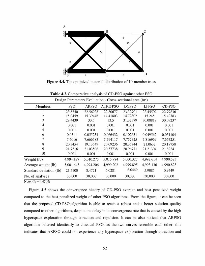
52
Figure 4.4. The optimized material distribution of 10-member truss.
Table 4.2. Comparative analysis of CD-PSO against other PSO
Design Parameters Evaluation - Cross-sectional area (in2)
Members PSO ARPSO ATRE-PSO DGPSO LFPSO CD-PSO
1 23.8750 22.56928 22.80677 23.32701 22.45509 22.79836 2 15.0459 15.39446 14.41803 14.72802 15.245 15.42783 3 29.4439 33.5 33.5 31.32379 30.08818 30.09237 4 0.001 0.001 0.001 0.001 0.001 0.001 5 0.001 0.001 0.001 0.001 0.001 0.001 6 0.0511 0.055231 0.066432 0.102651 0.049562 0.051104 7 7.6016 7.666583 7.794117 7.757325 7.816969 7.667251 8 20.3454 19.13549 20.09236 20.35744 21.0632 20.18758 9 21.7316 21.03506 20.57738 20.96771 21.21304 21.82241
10 0.001 0.001 0.001 0.001 0.001 0.001
Weight (lb) 4,994.187 5,010.275 5,015.984 5,000.327 4,992.614 4,990.583
Average weight (lb) 5,001.643 4,994.206 4,999.202 4,999.895 4,993.136 4,990.823
Standard deviation (lb) 21.5100 8.4721 6.0281 6.0449 5.9085 0.9449
No. of analyses 30,000 30,000 30,000 30,000 30,000 30,000 Note: (lb = 4.45 N)
Figure 4.5 shows the convergence history of CD-PSO average and best penalized weight
compared to the best penalized weight of other PSO algorithms. From the figure, it can be seen
that the proposed CD-PSO algorithm is able to reach a robust and a better solution quality
compared to other algorithms, despite the delay in its convergence rate that is caused by the high
hyperspace exploration through attraction and repulsion. It can be also noticed that ARPSO
algorithm behaved identically to classical PSO, as the two curves resemble each other, this
indicates that ARPSO could not experience any hyperspace exploration through attraction and
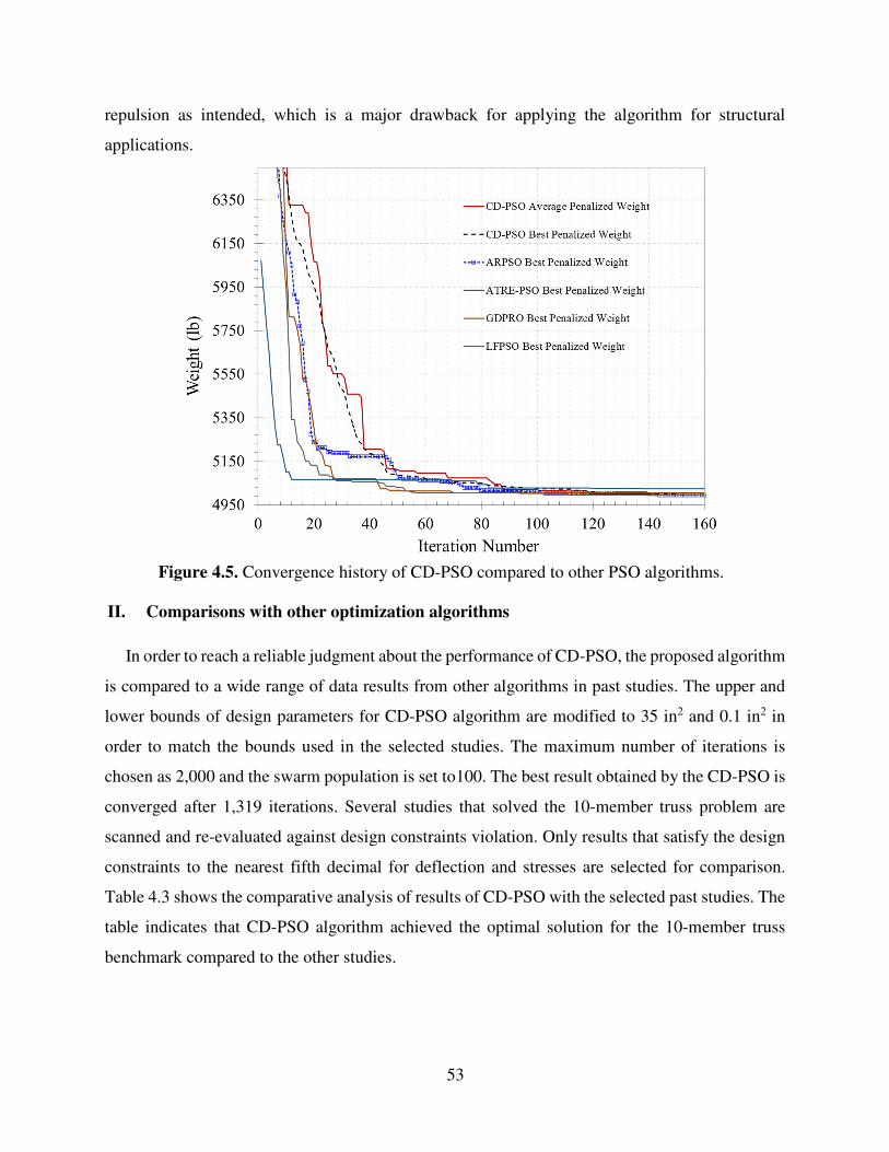
53
repulsion as intended, which is a major drawback for applying the algorithm for structural
applications.
Figure 4.5. Convergence history of CD-PSO compared to other PSO algorithms.
II. Comparisons with other optimization algorithms
In order to reach a reliable judgment about the performance of CD-PSO, the proposed algorithm
is compared to a wide range of data results from other algorithms in past studies. The upper and
lower bounds of design parameters for CD-PSO algorithm are modified to 35 in2 and 0.1 in2 in
order to match the bounds used in the selected studies. The maximum number of iterations is
chosen as 2,000 and the swarm population is set to100. The best result obtained by the CD-PSO is
converged after 1,319 iterations. Several studies that solved the 10-member truss problem are
scanned and re-evaluated against design constraints violation. Only results that satisfy the design
constraints to the nearest fifth decimal for deflection and stresses are selected for comparison.
Table 4.3 shows the comparative analysis of results of CD-PSO with the selected past studies. The
table indicates that CD-PSO algorithm achieved the optimal solution for the 10-member truss
benchmark compared to the other studies.
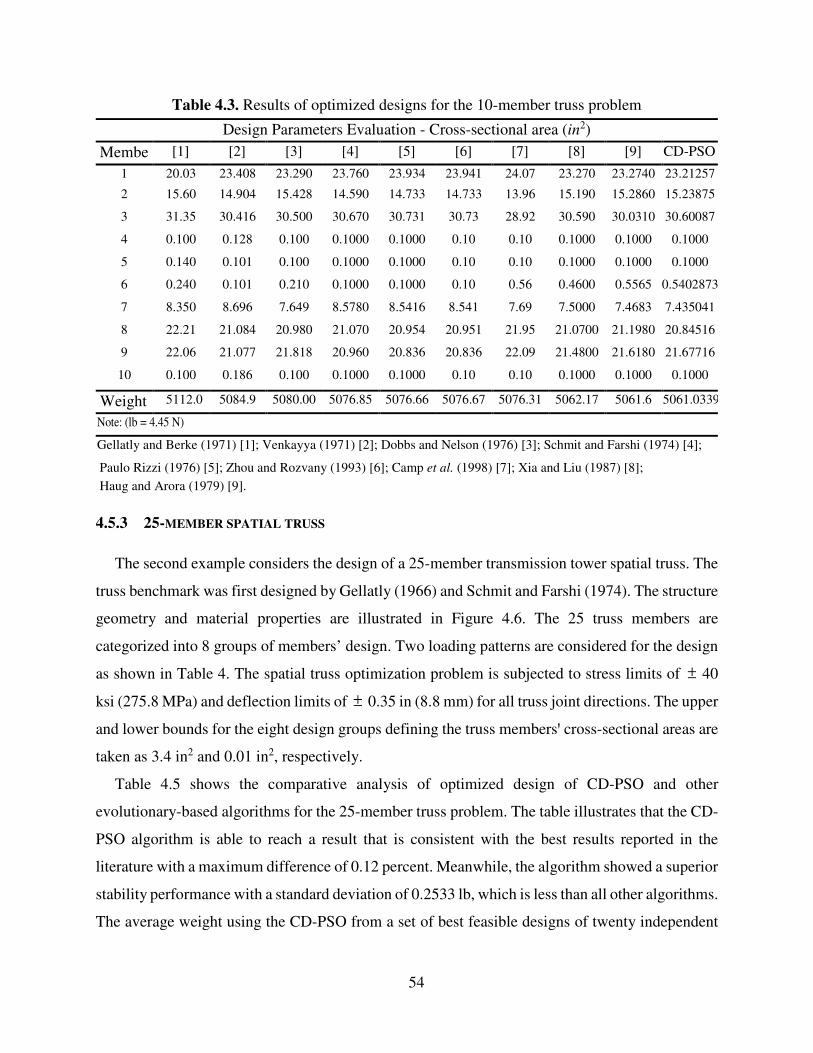
54
Table 4.3. Results of optimized designs for the 10-member truss problem
Design Parameters Evaluation - Cross-sectional area (in2)
Membe [1] [2] [3] [4] [5] [6] [7] [8] [9] CD-PSO
1 20.03 23.408 23.290 23.760 23.934 23.941 24.07 23.270 23.2740 23.21257
2 15.60 14.904 15.428 14.590 14.733 14.733 13.96 15.190 15.2860 15.23875
3 31.35 30.416 30.500 30.670 30.731 30.73 28.92 30.590 30.0310 30.60087
4 0.100 0.128 0.100 0.1000 0.1000 0.10 0.10 0.1000 0.1000 0.1000
5 0.140 0.101 0.100 0.1000 0.1000 0.10 0.10 0.1000 0.1000 0.1000
6 0.240 0.101 0.210 0.1000 0.1000 0.10 0.56 0.4600 0.5565 0.5402873
7 8.350 8.696 7.649 8.5780 8.5416 8.541 7.69 7.5000 7.4683 7.435041
8 22.21 21.084 20.980 21.070 20.954 20.951 21.95 21.0700 21.1980 20.84516
9 22.06 21.077 21.818 20.960 20.836 20.836 22.09 21.4800 21.6180 21.67716
10 0.100 0.186 0.100 0.1000 0.1000 0.10 0.10 0.1000 0.1000 0.1000
Weight 5112.0 5084.9 5080.00 5076.85 5076.66 5076.67 5076.31 5062.17 5061.6 5061.0339
Note: (lb = 4.45 N)
Gellatly and Berke (1971) [1]; Venkayya (1971) [2]; Dobbs and Nelson (1976) [3]; Schmit and Farshi (1974) [4];
Paulo Rizzi (1976) [5]; Zhou and Rozvany (1993) [6]; Camp et al. (1998) [7]; Xia and Liu (1987) [8]; Haug and Arora (1979) [9].
4.5.3 25-MEMBER SPATIAL TRUSS
The second example considers the design of a 25-member transmission tower spatial truss. The
truss benchmark was first designed by Gellatly (1966) and Schmit and Farshi (1974). The structure
geometry and material properties are illustrated in Figure 4.6. The 25 truss members are
categorized into 8 groups of members’ design. Two loading patterns are considered for the design
as shown in Table 4. The spatial truss optimization problem is subjected to stress limits of ± 40
ksi (275.8 MPa) and deflection limits of ± 0.35 in (8.8 mm) for all truss joint directions. The upper
and lower bounds for the eight design groups defining the truss membersꞌ cross-sectional areas are
taken as 3.4 in2 and 0.01 in2, respectively.
Table 4.5 shows the comparative analysis of optimized design of CD-PSO and other
evolutionary-based algorithms for the 25-member truss problem. The table illustrates that the CD-
PSO algorithm is able to reach a result that is consistent with the best results reported in the
literature with a maximum difference of 0.12 percent. Meanwhile, the algorithm showed a superior
stability performance with a standard deviation of 0.2533 lb, which is less than all other algorithms.
The average weight using the CD-PSO from a set of best feasible designs of twenty independent
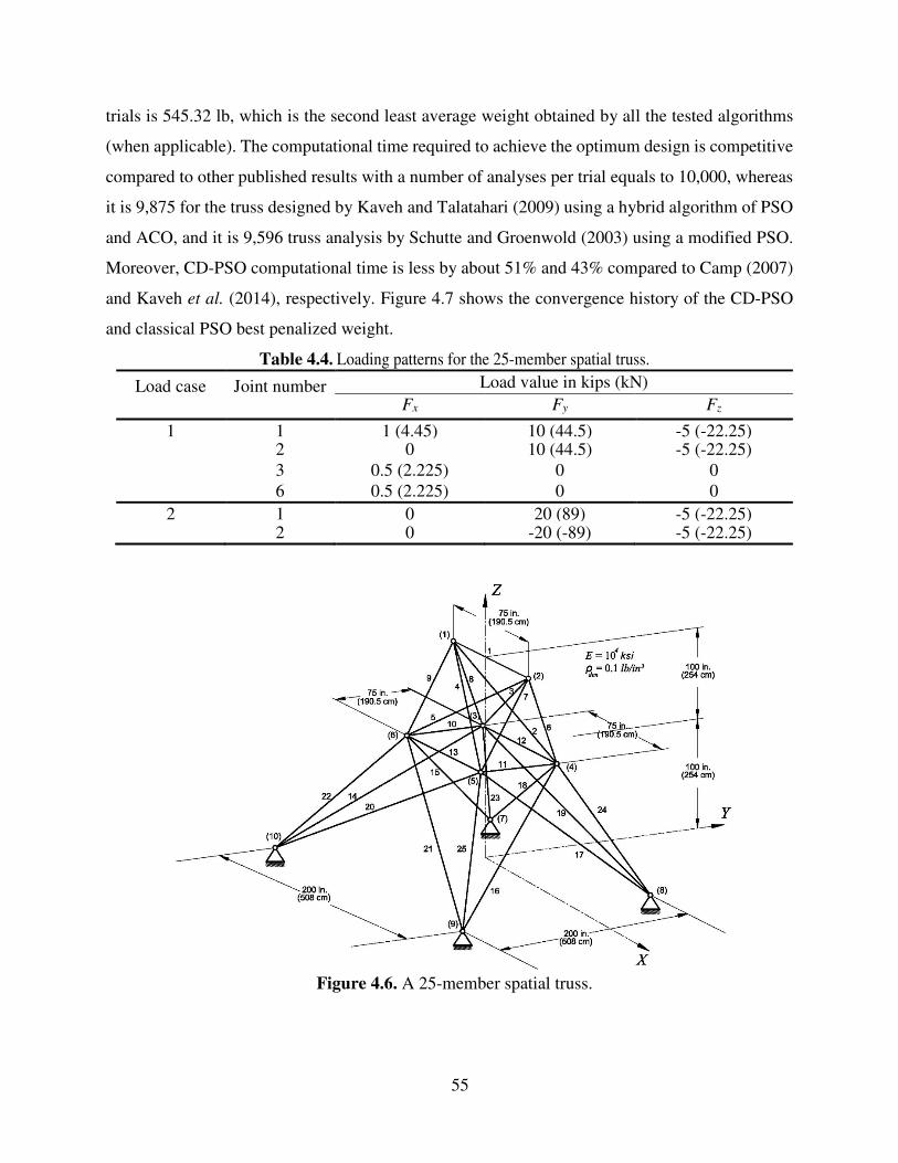
55
trials is 545.32 lb, which is the second least average weight obtained by all the tested algorithms
(when applicable). The computational time required to achieve the optimum design is competitive
compared to other published results with a number of analyses per trial equals to 10,000, whereas
it is 9,875 for the truss designed by Kaveh and Talatahari (2009) using a hybrid algorithm of PSO
and ACO, and it is 9,596 truss analysis by Schutte and Groenwold (2003) using a modified PSO.
Moreover, CD-PSO computational time is less by about 51% and 43% compared to Camp (2007)
and Kaveh et al. (2014), respectively. Figure 4.7 shows the convergence history of the CD-PSO
and classical PSO best penalized weight.
Table 4.4. Loading patterns for the 25-member spatial truss.
Load case Joint number Load value in kips (kN) Fx Fy Fz
1 1 1 (4.45) 10 (44.5) -5 (-22.25) 2 0 10 (44.5) -5 (-22.25) 3 0.5 (2.225) 0 0 6 0.5 (2.225) 0 0
2 1 0 20 (89) -5 (-22.25) 2 0 -20 (-89) -5 (-22.25)
Figure 4.6. A 25-member spatial truss.
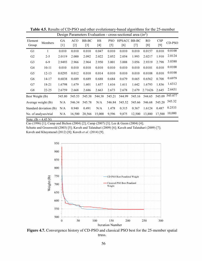
56
Table 4.5. Results of CD-PSO and other evolutionary-based algorithms for the 25-member
Design Parameters Evaluation - cross-sectional area (in2)
Element
Group Members
GA [1]
ACO [2]
BB-BC [3]
HS [4]
PSO [5]
HPSACO
[6] BB-BC
[7] RO [8]
CSP [9]
CD-PSO
G1 1 0.010 0.010 0.010 0.047 0.010 0.010 0.010 0.0157 0.010 0.0100
G2 2-5 2.0119 2.000 2.092 2.022 2.052 2.054 1.993 2.0217 1.910 2.0124
G3 6-9 2.9493 2.966 2.964 2.950 3.001 3.008 3.056 2.9319 2.798 3.0380
G4 10-11 0.010 0.010 0.010 0.010 0.010 0.010 0.010 0.0101 0.010 0.0100
G5 12-13 0.0295 0.012 0.010 0.014 0.010 0.010 0.010 0.0108 0.010 0.0100
G6 14-17 0.6838 0.689 0.689 0.688 0.684 0.679 0.665 0.6562 0.708 0.6979
G7 18-21 1.6798 1.679 1.601 1.657 1.616 1.611 1.642 1.6793 1.836 1.6312
G8 22-25 2.6759 2.668 2.686 2.663 2.673 2.678 2.679 2.71626 2.645 2.6431
Best Weight (lb) 545.80 545.53 545.38 544.38 545.21 544.99 545.16 544.65 545.09 545.077
Average weight (lb) N/A 546.34 545.78 N/A 546.84 545.52 545.66 546.68 545.20 545.32
Standard deviation (lb) N/A 0.940 0.491 N/A 1.478 0.315 0.367 1.6124 0.487 0.2533
No. of analyses/trial N/A 16,500 20,566 15,000 9,596 9,875 12,500 13,880 17,500 10,000
Note: (lb = 4.45 N) Cao (1996) [1]; Camp and Bichon (2004) [2]; Camp (2007) [3]; Lee & Geem (2004) [4]; Schutte and Groenwold (2003) [5]; Kaveh and Talatahari (2009) [6]; Kaveh and Talatahari (2009) [7]; Kaveh and Khayatazad (2012) [8]; Kaveh et al. (2014) [9].
Figure 4.7. Convergence history of CD-PSO and classical PSO best for the 25-member spatial truss.
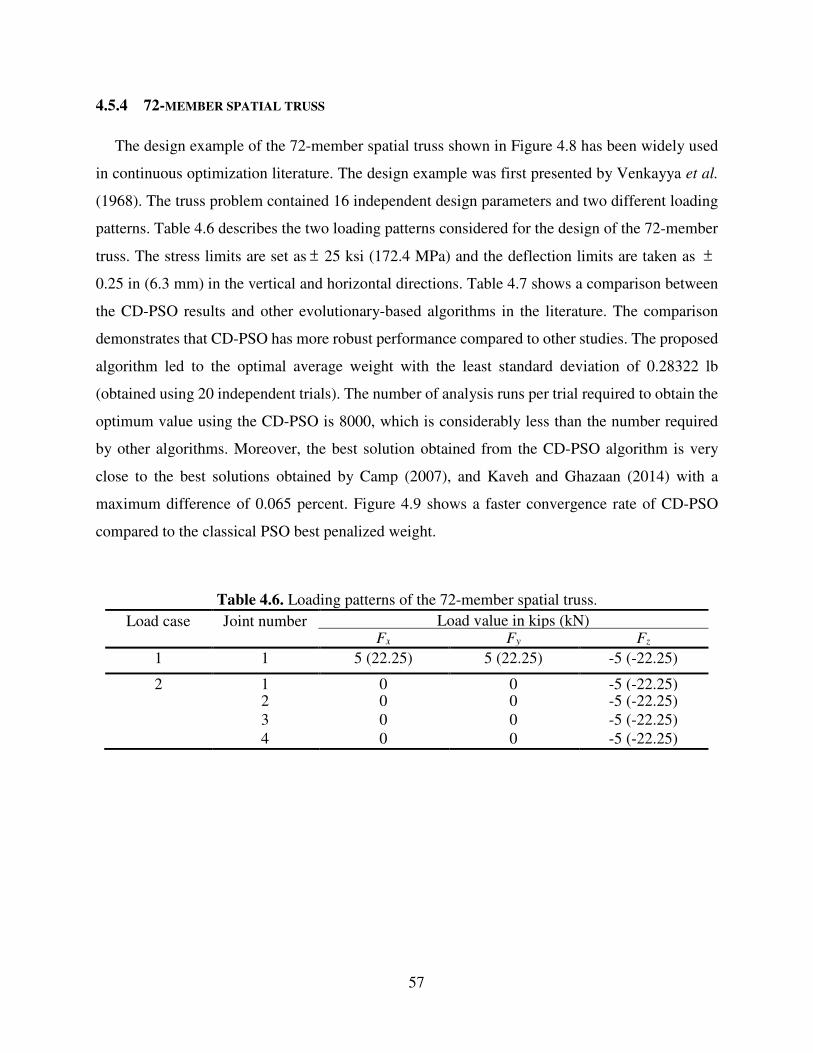
57
4.5.4 72-MEMBER SPATIAL TRUSS
The design example of the 72-member spatial truss shown in Figure 4.8 has been widely used
in continuous optimization literature. The design example was first presented by Venkayya et al.
(1968). The truss problem contained 16 independent design parameters and two different loading
patterns. Table 4.6 describes the two loading patterns considered for the design of the 72-member
truss. The stress limits are set as ± 25 ksi (172.4 MPa) and the deflection limits are taken as ±
0.25 in (6.3 mm) in the vertical and horizontal directions. Table 4.7 shows a comparison between
the CD-PSO results and other evolutionary-based algorithms in the literature. The comparison
demonstrates that CD-PSO has more robust performance compared to other studies. The proposed
algorithm led to the optimal average weight with the least standard deviation of 0.28322 lb
(obtained using 20 independent trials). The number of analysis runs per trial required to obtain the
optimum value using the CD-PSO is 8000, which is considerably less than the number required
by other algorithms. Moreover, the best solution obtained from the CD-PSO algorithm is very
close to the best solutions obtained by Camp (2007), and Kaveh and Ghazaan (2014) with a
maximum difference of 0.065 percent. Figure 4.9 shows a faster convergence rate of CD-PSO
compared to the classical PSO best penalized weight.
Table 4.6. Loading patterns of the 72-member spatial truss. Load case Joint number Load value in kips (kN)
Fx Fy Fz
1 1 5 (22.25) 5 (22.25) -5 (-22.25)
2 1 0 0 -5 (-22.25) 2 0 0 -5 (-22.25) 3 0 0 -5 (-22.25) 4 0 0 -5 (-22.25)
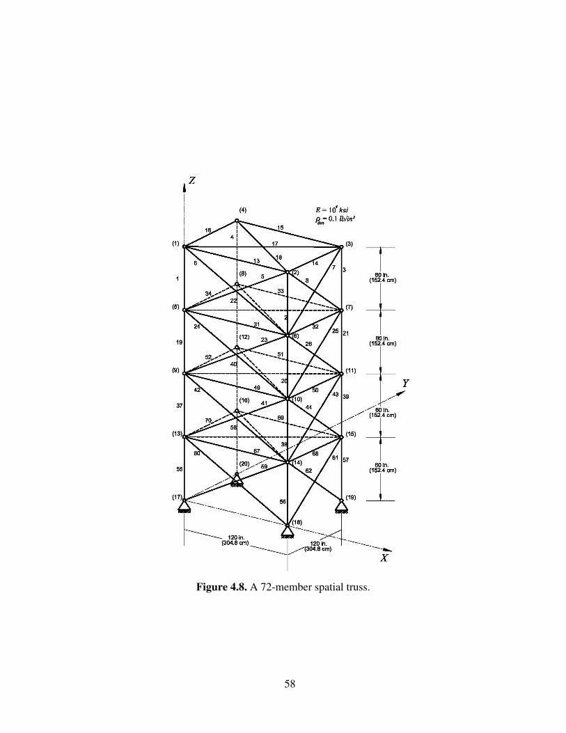
58
Figure 4.8. A 72-member spatial truss.
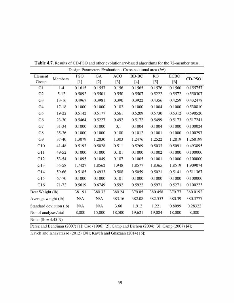
59
Table 4.7. Results of CD-PSO and other evolutionary-based algorithms for the 72-member truss.
Design Parameters Evaluation - Cross-sectional area (in2)
Element Group
Members PSO [1]
GA [2]
ACO [3]
BB-BC [4]
RO [5]
ECBO [6]
CD-PSO
G1 1-4 0.1615 0.1557 0.156 0.1565 0.1576 0.1560 0.155757G2 5-12 0.5092 0.5501 0.550 0.5507 0.5222 0.5572 0.550307
G3 13-16 0.4967 0.3981 0.390 0.3922 0.4356 0.4259 0.432478
G4 17-18 0.1000 0.1000 0.102 0.1000 0.1004 0.1000 0.530810
G5 19-22 0.5142 0.5177 0.561 0.5209 0.5730 0.5312 0.590520
G6 23-30 0.5464 0.5227 0.492 0.5172 0.5499 0.5173 0.517241
G7 31-34 0.1000 0.1000 0.1 0.1004 0.1004 0.1000 0.100024
G8 35-36 0.1000 0.1000 0.100 0.1012 0.1001 0.1000 0.100297
G9 37-40 1.3079 1.2830 1.303 1.2476 1.2522 1.2819 1.268199
G10 41-48 0.5193 0.5028 0.511 0.5269 0.5033 0.5091 0.493895
G11 49-52 0.1000 0.1000 0.101 0.1000 0.1002 0.1000 0.100000
G12 53-54 0.1095 0.1049 0.107 0.1005 0.1001 0.1000 0.100000
G13 55-58 1.7427 1.8562 1.948 1.8577 1.8365 1.8519 1.909074
G14 59-66 0.5185 0.4933 0.508 0.5059 0.5021 0.5141 0.511367
G15 67-70 0.1000 0.1000 0.101 0.1000 0.1000 0.1000 0.100000
G16 71-72 0.5619 0.6749 0.592 0.5922 0.5971 0.5271 0.100223
Best Weight (lb) 381.91 380.32 380.24 379.85 380.458 379.77 380.0192
Average weight (lb) N/A N/A 383.16 382.08 382.553 380.39 380.3777
Standard deviation (lb) N/A N/A 3.66 1.912 1.221 0.8099 0.28322
No. of analyses/trial 8,000 15,000 18,500 19,621 19,084 18,000 8,000
Note: (lb = 4.45 N)
Perez and Behdinan (2007) [1]; Cao (1996) [2]; Camp and Bichon (2004) [3]; Camp (2007) [4];
Kaveh and Khayatazad (2012) [38]; Kaveh and Ghazaan (2014) [6];
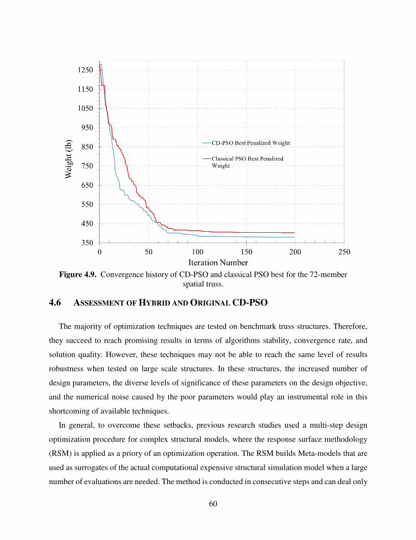
60
4.6 ASSESSMENT OF HYBRID AND ORIGINAL CD-PSO
The majority of optimization techniques are tested on benchmark truss structures. Therefore,
they succeed to reach promising results in terms of algorithms stability, convergence rate, and
solution quality. However, these techniques may not be able to reach the same level of results
robustness when tested on large scale structures. In these structures, the increased number of
design parameters, the diverse levels of significance of these parameters on the design objective,
and the numerical noise caused by the poor parameters would play an instrumental role in this
shortcoming of available techniques.
In general, to overcome these setbacks, previous research studies used a multi-step design
optimization procedure for complex structural models, where the response surface methodology
(RSM) is applied as a priory of an optimization operation. The RSM builds Meta-models that are
used as surrogates of the actual computational expensive structural simulation model when a large
number of evaluations are needed. The method is conducted in consecutive steps and can deal only
Figure 4.9. Convergence history of CD-PSO and classical PSO best for the 72-member spatial truss.
61
with continuous design optimization of complex structures. In the current research, CD-PSO and
hybridized CD-PSO with RSM are studied and applied on a large-scale structure, namely the
deployable bridge described in Chapter 3, in order to perform the optimization operation in a single
step, reduce the computational cost, and propose the method as a candidate for discrete
optimization of complex structural models. The RSM technique and its integration with CD-PSO
technique are clarified in the coming subsection.
The numerical results of testing CD-PSO and hybrid CD-PSO are compared with classical PSO
and GA results that are obtained in chapter 3 while considering all the design parameters.
Moreover, they are compared with classical PSO-S results (“S” stands for significant design
parameters), where only design parameters with sufficient influence on minimizing the weight of
the bridge structure are considered. These design parameters are determined through sensitivity
analysis of random trials. This will confirm the effectiveness of CD-PSO and the hybrid CD-PSO
in probing wide feasible areas in hyperspace to speed up the convergence rate and achieve
promising results.
4.6.1 RESPONSE SURFACE METHODOLOGY (RSM)
The response surface methodology (RSM) is an integration of mathematical and statistical
techniques that is generally used as a prior procedure to the planning of a complex optimization
operation. The method proposed by Box and Wilson (1951) can be applied when the analysis of
physical or numerical design problems involves a considerable number of design parameters. The
main function of RSM is to distinguish the influence of these design parameters on the design
objective. This would help the designer to eliminate the parameters with minor influence in order
to simplify the optimization process.
In general, the RSM integrates both the Design of Experiments (DOE) and the Response
Surface Analysis (RSA) techniques. First, the DOE is conducted to create multiple design trials
that randomly experiment the design parameters for a further classification. Out of this sampling
pool of design trials, a set of feasible designs is built through FE analysis for every design point in
the sampling pool. Random, Quasi-Random, Factorial, Placket-Burman designs, Latin hypercube
sampling and orthogonal arrays (Taguchi or Fisher) are examples of DOE sampling techniques
(Myers et al., 2009; Giunta et al., 2003; Santner et al., 2013; and Koehler and Owen, 1996). The
second step conducts a Response Surface Analysis (RSA) to interpolate the available data in order
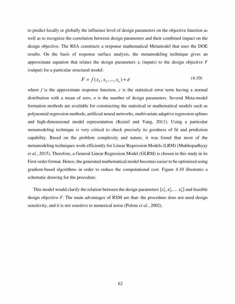
62
to predict locally or globally the influence level of design parameters on the objective function as
well as to recognize the correlation between design parameters and their combined impact on the
design objective. The RSA constructs a response mathematical Metamodel that uses the DOE
results. On the basis of response surface analysis, the metamodeling technique gives an
approximate equation that relates the design parameters xi (inputs) to the design objective F
(output) for a particular structural model:
ε+= ) ..., , ,( n21 xxxfF (4.10)
where f is the approximate response function, ε is the statistical error term having a normal
distribution with a mean of zero, n is the number of design parameters. Several Meta-model
formation methods are available for constructing the statistical or mathematical models such as
polynomial regression methods, artificial neural networks, multivariate adaptive regression splines
and high-dimensional model representation (Koziel and Yang, 2011). Using a particular
metamodeling technique is very critical to check precisely its goodness of fit and prediction
capability. Based on the problem complexity and nature, it was found that most of the
metamodeling techniques work efficiently for Linear Regression Models (LRM) (Mukhopadhyay
et al., 2015). Therefore, a General Linear Regression Model (GLRM) is chosen in this study in its
First-order format. Hence, the generated mathematical model becomes easier to be optimized using
gradient-based algorithms in order to reduce the computational cost. Figure 4.10 illustrates a
schematic drawing for the procedure.
This model would clarify the relation between the design parameters Ax1i , �2
i , …�ni B and feasible
design objective F. The main advantages of RSM are that: the procedure does not need design
sensitivity, and it is not sensitive to numerical noise (Poloni et al., 2002).
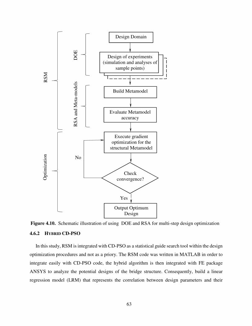
63
Figure 4.10. Schematic illustration of using DOE and RSA for multi-step design optimization
4.6.2 HYBRID CD-PSO
In this study, RSM is integrated with CD-PSO as a statistical guide search tool within the design
optimization procedures and not as a priory. The RSM code was written in MATLAB in order to
integrate easily with CD-PSO code, the hybrid algorithm is then integrated with FE package
ANSYS to analyze the potential designs of the bridge structure. Consequently, build a linear
regression model (LRM) that represents the correlation between design parameters and their
Design Domain
Build Metamodel
Design of experiments (simulation and analyses of
sample points)
Evaluate Metamodel accuracy
Execute gradient optimization for the
structural Metamodel
Check convergence?
Output Optimum Design
No o
Yes o
RSM
O
ptim
izat
ion
DO
E
RSA
and
Met
a-m
odel
s
64
influence on the design objective. The strategy of RSM implementation within the CD-PSO can
be described as follows:
Step 1. Generate random population using the following equation:
( )Lj
Uj
Kij
Lj
1Kij xxrxx −+=+ ),(),( (4.11)
where ��(5,�)is a random value between 0 and 1, xjUand xj
L are user–defined upper and lower bounds
of the design parameter xj . In this step, all the design parameters are considered for structural
design optimization.
Step 2. Disburse the swarm cloud in hyperspace to probe the good solutions and control the swarm
attraction and repulsion using the equations (4.2), (4.5), and (4.6). A matrix of only feasible design
points for the repelled particles is created. These data will be considered as the random samples
forming DOE in hyperspace. In this case, the particle’s encoded parameters are of random values
and not driven by the optimization formulas.
Step 3. Conduct a sensitivity analysis for the feasible design points using RSM, namely, DOE and
RSA, when any of the following conditions is satisfied:
a) If the best fitness is not improved,
b) If no repulsion phases occur,
c) Or if the solution diverges from the global best within a specific number of trials (chosen
as 1/6th of the travel history),
Step 4. Construct a First-order linear regression models (Kutner et al., 2004):
i
N
1j
i
jji
dv
xbby ε+⋅+= ∑=
o (4.12)
where ε is the error observed in the feasible response yi for the ith
particle data, and b is the
regression coefficients of the jth dimension in hyperspace. The value of b represents the change in
the design objective resulting from one unit change in the design parameter after fixing all the
other parameters, whereas b is expressed in the same unit of the design parameter. In order to
integrate Equation 4.12 with CD-PSO in MATLAB, the equation has to be defined in a matrix
form as follows:
ε1N11N1NN1N sampledvdvsamplesample
b××++××
+⋅=)()(
XY (4.13)

65
Where:
=×
sample
sample
N
2
1
1N
y
y
y
Y M
,
=+×
dvsamplesamplesample
dv
dv
dvsample
NN2N1N
N22221
N11211
1NN
xxx1
xxx1
xxx1
X
L
MMMM
L
L
)(
,
=×+
dv
dv
N
1
0
11N
b
b
b
b M)(
, and
=×
sample
sample
N
2
1
1N
ε
ε
ε
ε M
where Y is a vector of the design objectives’ values, X is a matrix of a column of 1 and columns of
Ndv parameters, in which it represents the design matrix of a set of value combinations of encoded
design parameters, Nsample is the number of feasible design points generated during repulsion, b is
a vector of regression coefficients, and ɛ is a vector of the error observed.
Step 5. Estimate the regression coefficients, fitted values, and residuals of errors of the model
a) The matrix b can be calculated as follows:
( ) YXXXb1
11Ndv
′′ ⋅−=×+ )(
(4.14)
where �P is the transpose of matrix X.
b) Calculate the hat matrix H using:
( ) XXXXH1
samplesample NN
′′ ⋅−=×
(4.15)
c) Calculate the vector of fitted values Qand the vector of residual terms e using:
HYXbY1Nsample
==×
ˆ (4.16)
YH1YY11N dv
−=−=
×+
ˆ)(
e (4.17)
d) Calculate matrix of standardized regression coefficients β using:
( )( )i
ij
iiystd
xstdb=β
(4.18)
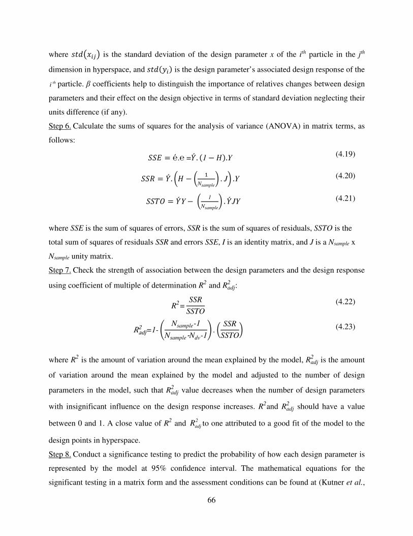
66
where RST�5�� is the standard deviation of the design parameter x of the ith particle in the jth
dimension in hyperspace, and RST(U5) is the design parameter’s associated design response of the
thi particle. β coefficients help to distinguish the importance of relatives changes between design
parameters and their effect on the design objective in terms of standard deviation neglecting their
units difference (if any).
Step 6. Calculate the sums of squares for the analysis of variance (ANOVA) in matrix terms, as
follows:
&&V = ℮́.℮ =QP . (1− X).Y (4.19)
&&Y = QP . ZX − Z �Nsample
[ .J[ .Y (4.20)
&&\] = QPY −Z 1
Nsample
[ . QP JY (4.21)
where SSE is the sum of squares of errors, SSR is the sum of squares of residuals, SSTO is the
total sum of squares of residuals SSR and errors SSE, I is an identity matrix, and J is a Nsample x
Nsample unity matrix.
Step 7. Check the strength of association between the design parameters and the design response
using coefficient of multiple of determination R2 and Radj2 :
R2=
SSR
SSTO (4.22)
Radj2 =1-a Nsample-1
Nsample-Ndv-1c . Z SSR
SSTO[ (4.23)
where R2 is the amount of variation around the mean explained by the model, Radj2 is the amount
of variation around the mean explained by the model and adjusted to the number of design
parameters in the model, such that Radj2 value decreases when the number of design parameters
with insignificant influence on the design response increases. R2and Radj
2 should have a value
between 0 and 1. A close value of R2 and 2
adjR to one attributed to a good fit of the model to the
design points in hyperspace.
Step 8. Conduct a significance testing to predict the probability of how each design parameter is
represented by the model at 95% confidence interval. The mathematical equations for the
significant testing in a matrix form and the assessment conditions can be found at (Kutner et al.,

67
2004).
Step 9. Normalize the unstandardized coefficients of all the design parameters with respect to the
design parameter that has the highest influence on the design objective, given the design
parameters with the highest influence an assumed value of 100%.
Step 10. Classify the design parameters according to their associated normalized coefficients
according to Table 4.8. The values in Table 4.8 are considered as a measure of the design
parameters’ influence on the design objective.
Table 4.8. Influence classification of the effect of design parameters on the design objective
Influence classification ω (%)
Very significant 10 ≤ ω ≤ 100
Significant 5 ≤ ω < 10
Minor 2 ≤ ω < 5
Negligible 0 ≤ ω < 2
Step 11. Based on the design parameter’s classification in step 10. A decision is made, such that
all design parameters with poor influence or with a model relation less than 95% confidence will
be mutated and fixed to their corresponding values in the global best. The remaining parameters
will be updated using equations (4.1) and (4.2) to allow the swarm particles to find better positions
in hyperspace to the end of travel history.
Step 12. Before continuing the search, disperse randomly the swarm particles to allow a wide scan
for the design space under the effect of only the significant design parameters. Figure 4.11 shows
a flowchart drawing of the hybrid CD-PSO algorithm with RSM. A pseudocode for the CD-PSO
algorithm is created to clarify Hybrid CD-PSO algorithm and it is illustrated in appendix B-1.
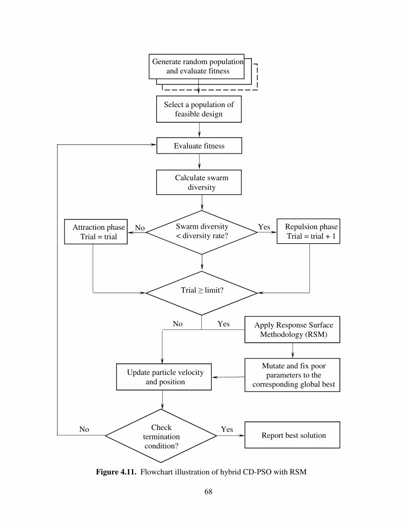
68
Figure 4.11. Flowchart illustration of hybrid CD-PSO with RSM
Repulsion phase Trial = trial + 1
Attraction phase Trial = trial
Yes oNo o
Select a population of feasible design
Generate random population and evaluate fitness
Evaluate fitness
Calculate swarm diversity
Swarm diversity < diversity rate?
Trial ≥ limit?
Update particle velocity and position
No o Yes o Apply Response Surface Methodology (RSM)
Mutate and fix poor parameters to the
corresponding global best
Check termination condition?
Report best solution Yes o No o
69
4.6.3 NUMERICAL RESULTS
The application of GA resulted in a bridge weight of 9.245 tons (20381 lb) with an
enhancement of 29.4% from the base conventional design 13.099 tons (28878 lb). On the other
hand, the application of PSO-A while considering the whole set of design parameters resulted in
8.929 tons (19685 lb), hence, an improvement of 31.8% from the base conventional design weight
is achieved. Design parameters’ values obtained by both algorithms GA and PSO-A are listed in
Table 4.9.
In order to apply PSO-S (“S” stands for significant design parameters) for minimizing the
weight of the bridge structure. The previously obtained 31 feasible designs in section 3.2.3.2 are
used to create a pool of design points for further sensitivity analysis of the design parameters. The
aforementioned steps from 4 to 10 are applied to estimate the influence of the design parameters
on the design objective through constructing a linear regression model. Table 4.10 shows the
unstandardized, standardized, and the probability value of how each design parameter is
represented by the model. The regression model developed showed a strength of association R2adj
of 0.9998, which indicates an excellent fit of the model to the design points in hyperspace. The
design parameters’ coefficients are normalized to a percent value of the highest unstandardized
coefficient and denoted as ω in Table 4.10. Amongst the whole design parameters, it was found
that eighteen design parameters have sufficient influence more than 2% on the design objective
based on the classification listed in Table 4.8. Moreover, significant design parameters with a
probability value not less than 95% confidence interval are only considered for velocity updates
when applying PSO-S. Finally, the application of PSO-S resulted in a bridge weight of 10.306 tons
(22720 lb) and a minimized weight/capacity ratio of only 21.326 %. On the other hand, CD-PSO
achieved a decrease in weight/capacity ratio of 33.2 percent based on a deployable bridge weight
of 8.773 tons (19342 lb), while Hybrid CD-PSO with RSM achieved the best reduction in
weight/capacity ratio by 34.3 percent with a total bridge weight of 8.606 tons (18972 lb). Table
4.9 shows the parameters’ values of the best design achieved by CD-PSO and hybrid CD-PSO
with RSM, while Table 4.11 lists the LRM coefficients and percent of parameters significance
achieved by Hybrid CD-PSO with RSM. Finally, Figure 4.12 shows the convergence history of
the four applied techniques.
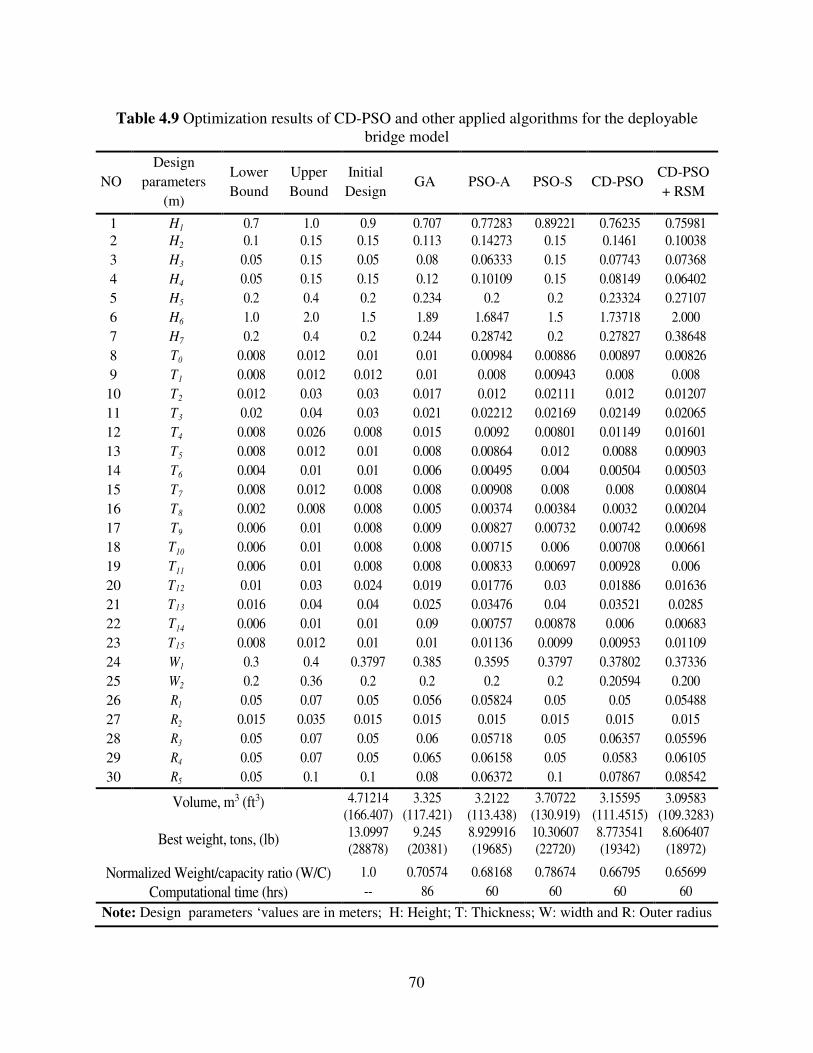
70
Table 4.9 Optimization results of CD-PSO and other applied algorithms for the deployable bridge model
NO Design
parameters (m)
Lower Bound
Upper Bound
Initial Design
GA PSO-A PSO-S CD-PSO CD-PSO + RSM
1 H1 0.7 1.0 0.9 0.707 0.77283 0.89221 0.76235 0.75981 2 H2 0.1 0.15 0.15 0.113 0.14273 0.15 0.1461 0.10038 3 H3 0.05 0.15 0.05 0.08 0.06333 0.15 0.07743 0.07368 4 H4 0.05 0.15 0.15 0.12 0.10109 0.15 0.08149 0.06402 5 H5 0.2 0.4 0.2 0.234 0.2 0.2 0.23324 0.27107 6 H6 1.0 2.0 1.5 1.89 1.6847 1.5 1.73718 2.000 7 H7 0.2 0.4 0.2 0.244 0.28742 0.2 0.27827 0.38648 8 T0 0.008 0.012 0.01 0.01 0.00984 0.00886 0.00897 0.00826 9 T1 0.008 0.012 0.012 0.01 0.008 0.00943 0.008 0.008
10 T2 0.012 0.03 0.03 0.017 0.012 0.02111 0.012 0.01207 11 T3 0.02 0.04 0.03 0.021 0.02212 0.02169 0.02149 0.02065 12 T4 0.008 0.026 0.008 0.015 0.0092 0.00801 0.01149 0.01601 13 T5 0.008 0.012 0.01 0.008 0.00864 0.012 0.0088 0.00903 14 T6 0.004 0.01 0.01 0.006 0.00495 0.004 0.00504 0.00503 15 T7 0.008 0.012 0.008 0.008 0.00908 0.008 0.008 0.00804 16 T8 0.002 0.008 0.008 0.005 0.00374 0.00384 0.0032 0.00204 17 T9 0.006 0.01 0.008 0.009 0.00827 0.00732 0.00742 0.00698 18 T10 0.006 0.01 0.008 0.008 0.00715 0.006 0.00708 0.00661 19 T11 0.006 0.01 0.008 0.008 0.00833 0.00697 0.00928 0.006 20 T12 0.01 0.03 0.024 0.019 0.01776 0.03 0.01886 0.01636 21 T13 0.016 0.04 0.04 0.025 0.03476 0.04 0.03521 0.0285 22 T14 0.006 0.01 0.01 0.09 0.00757 0.00878 0.006 0.00683 23 T15 0.008 0.012 0.01 0.01 0.01136 0.0099 0.00953 0.01109 24 W1 0.3 0.4 0.3797 0.385 0.3595 0.3797 0.37802 0.37336 25 W2 0.2 0.36 0.2 0.2 0.2 0.2 0.20594 0.200 26 R1 0.05 0.07 0.05 0.056 0.05824 0.05 0.05 0.05488 27 R2 0.015 0.035 0.015 0.015 0.015 0.015 0.015 0.015 28 R3 0.05 0.07 0.05 0.06 0.05718 0.05 0.06357 0.05596 29 R4 0.05 0.07 0.05 0.065 0.06158 0.05 0.0583 0.06105 30 R5 0.05 0.1 0.1 0.08 0.06372 0.1 0.07867 0.08542
Volume, m3 (ft3) 4.71214 (166.407)
3.325 (117.421)
3.2122 (113.438)
3.70722 (130.919)
3.15595 (111.4515)
3.09583 (109.3283)
Best weight, tons, (lb) 13.0997 (28878)
9.245 (20381)
8.929916 (19685)
10.30607 (22720)
8.773541 (19342)
8.606407 (18972)
Normalized Weight/capacity ratio (W/C) 1.0 0.70574 0.68168 0.78674 0.66795 0.65699 Computational time (hrs) -- 86 60 60 60 60
Note: Design parameters ‘values are in meters; H: Height; T: Thickness; W: width and R: Outer radius
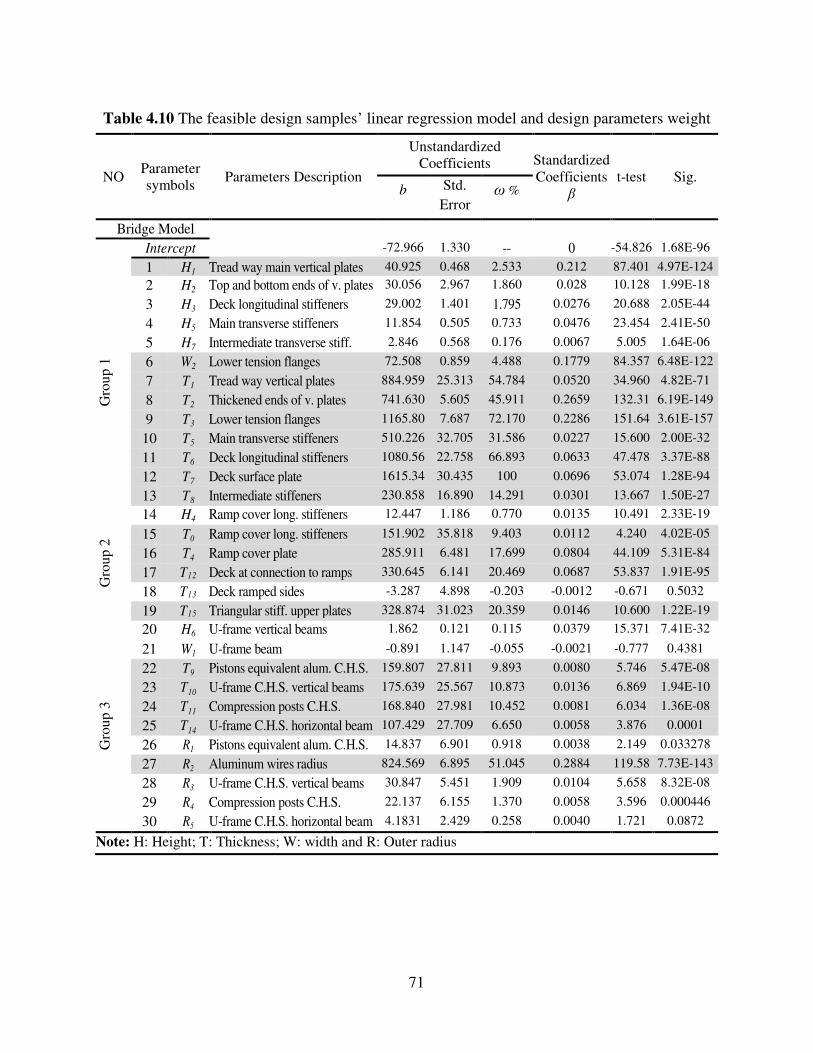
71
Table 4.10 The feasible design samples’ linear regression model and design parameters weight
NO Parameter symbols Parameters Description
Unstandardized Coefficients Standardized
Coefficients β
t-test Sig. b Std.
Error ω %
Bridge Model
Intercept -72.966 1.330 -- 0 -54.826 1.68E-96
Gro
up 1
1 H1 Tread way main vertical plates 40.925 0.468 2.533 0.212 87.401 4.97E-124
2 H2 Top and bottom ends of v. plates 30.056 2.967 1.860 0.028 10.128 1.99E-18
3 H3 Deck longitudinal stiffeners 29.002 1.401 1.795 0.0276 20.688 2.05E-44
4 H5 Main transverse stiffeners 11.854 0.505 0.733 0.0476 23.454 2.41E-50
5 H7 Intermediate transverse stiff. 2.846 0.568 0.176 0.0067 5.005 1.64E-06
6 W2 Lower tension flanges 72.508 0.859 4.488 0.1779 84.357 6.48E-122
7 T1 Tread way vertical plates 884.959 25.313 54.784 0.0520 34.960 4.82E-71
8 T2 Thickened ends of v. plates 741.630 5.605 45.911 0.2659 132.31 6.19E-149
9 T3 Lower tension flanges 1165.80 7.687 72.170 0.2286 151.64 3.61E-157
10 T5 Main transverse stiffeners 510.226 32.705 31.586 0.0227 15.600 2.00E-32
11 T6 Deck longitudinal stiffeners 1080.56 22.758 66.893 0.0633 47.478 3.37E-88
12 T7 Deck surface plate 1615.34 30.435 100 0.0696 53.074 1.28E-94
13 T8 Intermediate stiffeners 230.858 16.890 14.291 0.0301 13.667 1.50E-27
Gro
up 2
14 H4 Ramp cover long. stiffeners 12.447 1.186 0.770 0.0135 10.491 2.33E-19
15 T0 Ramp cover long. stiffeners 151.902 35.818 9.403 0.0112 4.240 4.02E-05
16 T4 Ramp cover plate 285.911 6.481 17.699 0.0804 44.109 5.31E-84
17 T12 Deck at connection to ramps 330.645 6.141 20.469 0.0687 53.837 1.91E-95
18 T13 Deck ramped sides -3.287 4.898 -0.203 -0.0012 -0.671 0.5032
19 T15 Triangular stiff. upper plates 328.874 31.023 20.359 0.0146 10.600 1.22E-19
Gro
up 3
20 H6 U-frame vertical beams 1.862 0.121 0.115 0.0379 15.371 7.41E-32
21 W1 U-frame beam -0.891 1.147 -0.055 -0.0021 -0.777 0.4381
22 T9 Pistons equivalent alum. C.H.S. 159.807 27.811 9.893 0.0080 5.746 5.47E-08
23 T10 U-frame C.H.S. vertical beams 175.639 25.567 10.873 0.0136 6.869 1.94E-10
24 T11 Compression posts C.H.S. 168.840 27.981 10.452 0.0081 6.034 1.36E-08
25 T14 U-frame C.H.S. horizontal beam 107.429 27.709 6.650 0.0058 3.876 0.0001
26 R1 Pistons equivalent alum. C.H.S. 14.837 6.901 0.918 0.0038 2.149 0.033278
27 R2 Aluminum wires radius 824.569 6.895 51.045 0.2884 119.58 7.73E-143
28 R3 U-frame C.H.S. vertical beams 30.847 5.451 1.909 0.0104 5.658 8.32E-08
29 R4 Compression posts C.H.S. 22.137 6.155 1.370 0.0058 3.596 0.000446
30 R5 U-frame C.H.S. horizontal beam 4.1831 2.429 0.258 0.0040 1.721 0.0872
Note: H: Height; T: Thickness; W: width and R: Outer radius
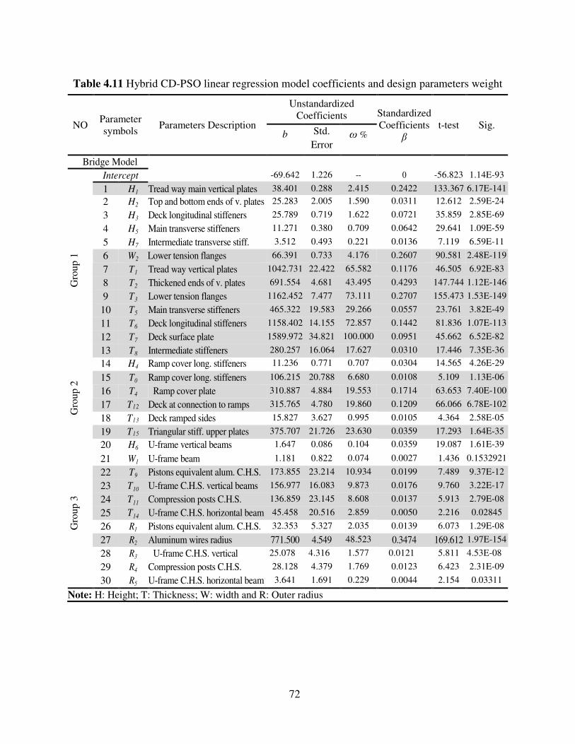
72
Table 4.11 Hybrid CD-PSO linear regression model coefficients and design parameters weight
NO Parameter symbols
Parameters Description
Unstandardized Coefficients Standardized
Coefficients β
t-test Sig. b Std.
Error ω %
Bridge Model
Intercept -69.642 1.226
-- 0 -56.823
1.14E-93
Gro
up 1
1 H1 Tread way main vertical plates 38.401 0.288
2.415 0.2422
133.367
6.17E-141 2 H2 Top and bottom ends of v. plates 25.283 2.005
1.590 0.0311
12.612
2.59E-24
3 H3 Deck longitudinal stiffeners 25.789 0.719
1.622 0.0721
35.859
2.85E-69 4 H5 Main transverse stiffeners 11.271
0.380
0.709 0.0642
29.641
1.09E-59
5 H7 Intermediate transverse stiff. 3.512
0.493
0.221 0.0136
7.119
6.59E-11 6 W2 Lower tension flanges 66.391 0.733 4.176 0.2607 90.581 2.48E-119
7 T1 Tread way vertical plates 1042.731 22.422 65.582 0.1176 46.505 6.92E-83
8 T2 Thickened ends of v. plates 691.554 4.681 43.495 0.4293 147.744 1.12E-146
9 T3 Lower tension flanges 1162.452 7.477 73.111 0.2707 155.473 1.53E-149
10 T5 Main transverse stiffeners 465.322 19.583 29.266 0.0557 23.761 3.82E-49
11 T6 Deck longitudinal stiffeners 1158.402 14.155 72.857 0.1442 81.836 1.07E-113
12 T7 Deck surface plate 1589.972 34.821 100.000 0.0951 45.662 6.52E-82
13 T8 Intermediate stiffeners 280.257 16.064 17.627 0.0310 17.446 7.35E-36
Gro
up 2
14 H4 Ramp cover long. stiffeners 11.236
0.771
0.707 0.0304
14.565
4.26E-29 15 T0 Ramp cover long. stiffeners 106.215 20.788 6.680 0.0108
5.109 1.13E-06
16 T4 Ramp cover plate 310.887 4.884 19.553 0.1714 63.653 7.40E-100
17 T12 Deck at connection to ramps 315.765 4.780 19.860 0.1209 66.066 6.78E-102
18 T13 Deck ramped sides 15.827 3.627 0.995 0.0105 4.364 2.58E-05
19 T15 Triangular stiff. upper plates 375.707 21.726 23.630 0.0359
17.293 1.64E-35
Gro
up 3
20 H6 U-frame vertical beams 1.647 0.086 0.104 0.0359
19.087 1.61E-39
21 W1 U-frame beam 1.181 0.822 0.074 0.0027
1.436 0.1532921
22 T9 Pistons equivalent alum. C.H.S. 173.855 23.214 10.934 0.0199 7.489 9.37E-12
23 T10 U-frame C.H.S. vertical beams 156.977 16.083 9.873 0.0176 9.760 3.22E-17
24 T11 Compression posts C.H.S. 136.859 23.145 8.608 0.0137 5.913 2.79E-08
25 T14 U-frame C.H.S. horizontal beam 45.458 20.516 2.859 0.0050 2.216 0.02845
26 R1 Pistons equivalent alum. C.H.S. 32.353 5.327 2.035 0.0139 6.073 1.29E-08
27 R2 Aluminum wires radius 771.500 4.549 48.523 0.3474 169.612 1.97E-154
28 R3 U-frame C.H.S. vertical 25.078 4.316 1.577 0.0121 5.811 4.53E-08
29 R4 Compression posts C.H.S. 28.128 4.379 1.769 0.0123 6.423 2.31E-09
30 R5 U-frame C.H.S. horizontal beam 3.641 1.691 0.229 0.0044 2.154 0.03311
Note: H: Height; T: Thickness; W: width and R: Outer radius
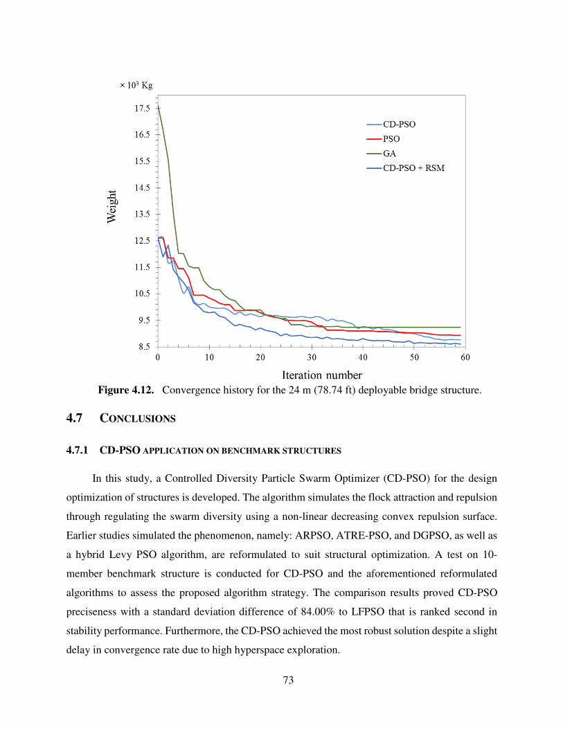
73
4.7 CONCLUSIONS
4.7.1 CD-PSO APPLICATION ON BENCHMARK STRUCTURES
In this study, a Controlled Diversity Particle Swarm Optimizer (CD-PSO) for the design
optimization of structures is developed. The algorithm simulates the flock attraction and repulsion
through regulating the swarm diversity using a non-linear decreasing convex repulsion surface.
Earlier studies simulated the phenomenon, namely: ARPSO, ATRE-PSO, and DGPSO, as well as
a hybrid Levy PSO algorithm, are reformulated to suit structural optimization. A test on 10-
member benchmark structure is conducted for CD-PSO and the aforementioned reformulated
algorithms to assess the proposed algorithm strategy. The comparison results proved CD-PSO
preciseness with a standard deviation difference of 84.00% to LFPSO that is ranked second in
stability performance. Furthermore, the CD-PSO achieved the most robust solution despite a slight
delay in convergence rate due to high hyperspace exploration.
Figure 4.12. Convergence history for the 24 m (78.74 ft) deployable bridge structure.
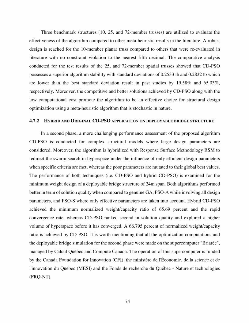
74
Three benchmark structures (10, 25, and 72-member trusses) are utilized to evaluate the
effectiveness of the algorithm compared to other meta-heuristic results in the literature. A robust
design is reached for the 10-member planar truss compared to others that were re-evaluated in
literature with no constraint violation to the nearest fifth decimal. The comparative analysis
conducted for the test results of the 25, and 72-member spatial trusses showed that CD-PSO
possesses a superior algorithm stability with standard deviations of 0.2533 lb and 0.2832 lb which
are lower than the best standard deviation result in past studies by 19.58% and 65.03%,
respectively. Moreover, the competitive and better solutions achieved by CD-PSO along with the
low computational cost promote the algorithm to be an effective choice for structural design
optimization using a meta-heuristic algorithm that is stochastic in nature.
4.7.2 HYBRID AND ORIGINAL CD-PSO APPLICATION ON DEPLOYABLE BRIDGE STRUCTURE
In a second phase, a more challenging performance assessment of the proposed algorithm
CD-PSO is conducted for complex structural models where large design parameters are
considered. Moreover, the algorithm is hybridized with Response Surface Methodology RSM to
redirect the swarm search in hyperspace under the influence of only efficient design parameters
when specific criteria are met, whereas the poor parameters are mutated to their global best values.
The performance of both techniques (i.e. CD-PSO and hybrid CD-PSO) is examined for the
minimum weight design of a deployable bridge structure of 24m span. Both algorithms performed
better in term of solution quality when compared to genuine GA, PSO-A while involving all design
parameters, and PSO-S where only effective parameters are taken into account. Hybrid CD-PSO
achieved the minimum normalized weight/capacity ratio of 65.69 percent and the rapid
convergence rate, whereas CD-PSO ranked second in solution quality and explored a higher
volume of hyperspace before it has converged. A 66.795 percent of normalized weight/capacity
ratio is achieved by CD-PSO. It is worth mentioning that all the optimization computations and
the deployable bridge simulation for the second phase were made on the supercomputer "Briarée",
managed by Calcul Québec and Compute Canada. The operation of this supercomputer is funded
by the Canada Foundation for Innovation (CFI), the ministère de l'Économie, de la science et de
l'innovation du Québec (MESI) and the Fonds de recherche du Québec - Nature et technologies
(FRQ-NT).

75
4.8 SUMMARY
In this chapter, the controlled diversity particle swarm CD-PSO and its hybrid version with
RSM are proposed. CD-PSO showed a satisfactory performance for the application of large-scale
structural design optimization. However, hybrid CD-PSO is more recommended for complex
structural optimization where a high varying influence of design parameters on the design
objective exists. From the analysis of the results, it can be shown that deployable bridge decks
contribute to more than 20% of the total bridge weight. Moreover, the design of these bridge decks
as the main bearing element of compression in deployable bridge structures is very critical, to
which it is the main focus of this study. Therefore, CD-PSO is chosen for maximizing the strength
and stiffness of the proposed bridge deck sandwich cores, whereas hybrid CD-PSO is kept for
future size and shape optimization of a scaled deployable bridge treadway. The following chapter
will present two different sandwich cores designed for the bridge deck, as well as demonstrate the
experimental program for testing the cores along with its numerical validation.
76
CHAPTER 5
Developing and Testing of New
Composite Decks 5.1 INTRODUCTION
In the recent decades, many research studies investigated replacing the deteriorated metallic or
concrete deck bridges with alternatives of composite FRP decks, such as Lopez et al. (1997), Brown
and Zureick (2001), Davalos et al. (2001), Zetterberg et al. (2001), Williams et al. (2003), Link
(2003), Keller and Gürtler (2005), Zhou et al. (2005), Liu (2007), Osei-Antwi et al. (2013), Keller
et al. (2014), Zhu and Lopez (2014), and Tuwair et al. (2015). On the other hand, Kosmatka et al.
(2000) and Robinson and Kosmatka (2008) investigated alternatives of high performance CFRP
deck systems that are characterized by higher strength to weight ratio for the application in the
Composite Assault Bridge (CAB) and the Composite Joint Assault Bridge (CJAB) deployable
systems, respectively. As a result of the increased demand for disaster aftermath bridge rapid
mobility, the current research investigates the performance of two alternatives of sandwich CFRP
cores which provides increased capacity to weight ratio compared to the core system of the CAB
bridge. Moreover, the CFRP cores’ design configuration is compared with two reproduced webbed
CFRP cores using the same design configuration and manufacturing procedure that are recently
developed by Robinson and Kosmatka (2008).
In this chapter, a review of different manufacturing techniques is presented followed by a
comparison between all the processing methods advantages and disadvantages. The design of the
proposed sandwich cores as well as a detailed description of each core are demonstrated; the CAB
bridge deck core and the two CFRP webbed cores developed by Robinson and Kosmatka (2008) are
briefly described. Followed by a description of the experimental test setups and the instrumentations
developed to evaluate the cores’ compression and shear strength; the experimental results are then
clarified. A finite element progressive failure analysis for the proposed sandwich cores is performed.
Finally, a numerical validation of the experimental results is summarized.
5
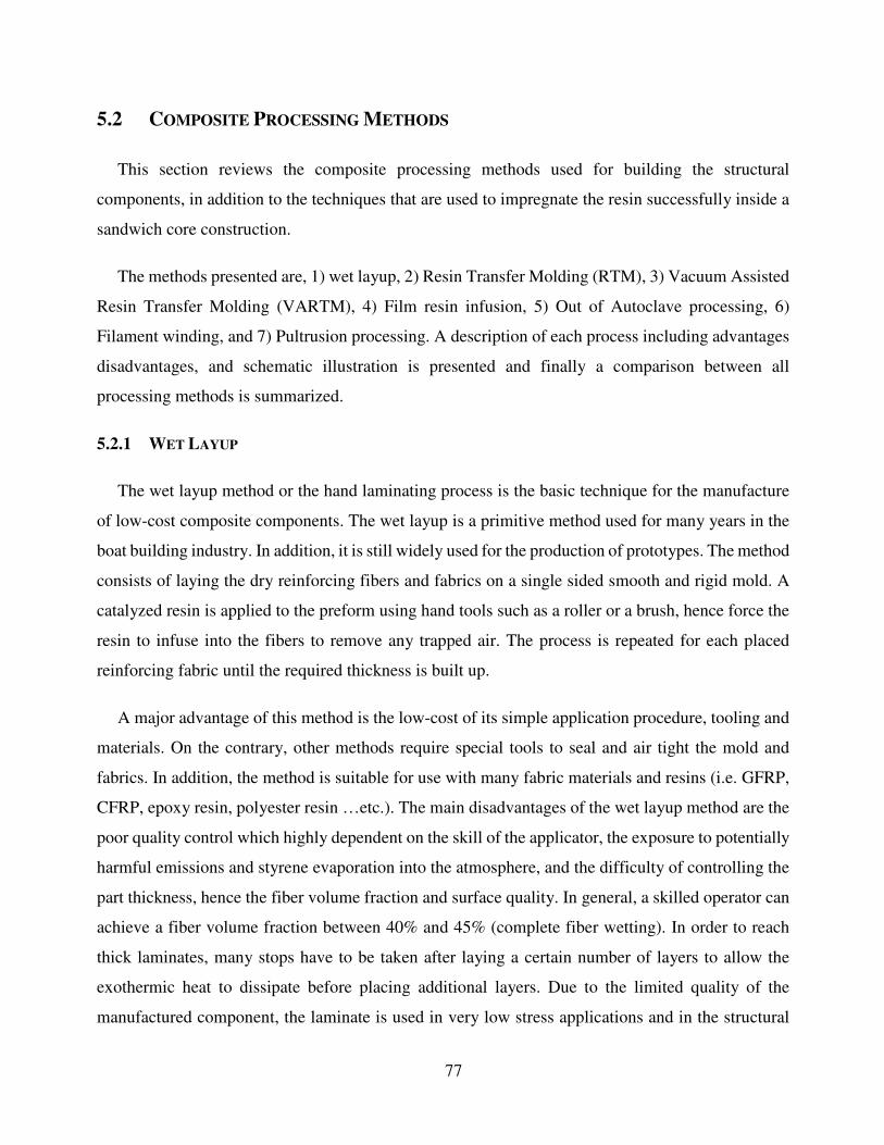
77
5.2 COMPOSITE PROCESSING METHODS
This section reviews the composite processing methods used for building the structural
components, in addition to the techniques that are used to impregnate the resin successfully inside a
sandwich core construction.
The methods presented are, 1) wet layup, 2) Resin Transfer Molding (RTM), 3) Vacuum Assisted
Resin Transfer Molding (VARTM), 4) Film resin infusion, 5) Out of Autoclave processing, 6)
Filament winding, and 7) Pultrusion processing. A description of each process including advantages
disadvantages, and schematic illustration is presented and finally a comparison between all
processing methods is summarized.
5.2.1 WET LAYUP
The wet layup method or the hand laminating process is the basic technique for the manufacture
of low-cost composite components. The wet layup is a primitive method used for many years in the
boat building industry. In addition, it is still widely used for the production of prototypes. The method
consists of laying the dry reinforcing fibers and fabrics on a single sided smooth and rigid mold. A
catalyzed resin is applied to the preform using hand tools such as a roller or a brush, hence force the
resin to infuse into the fibers to remove any trapped air. The process is repeated for each placed
reinforcing fabric until the required thickness is built up.
A major advantage of this method is the low-cost of its simple application procedure, tooling and
materials. On the contrary, other methods require special tools to seal and air tight the mold and
fabrics. In addition, the method is suitable for use with many fabric materials and resins (i.e. GFRP,
CFRP, epoxy resin, polyester resin …etc.). The main disadvantages of the wet layup method are the
poor quality control which highly dependent on the skill of the applicator, the exposure to potentially
harmful emissions and styrene evaporation into the atmosphere, and the difficulty of controlling the
part thickness, hence the fiber volume fraction and surface quality. In general, a skilled operator can
achieve a fiber volume fraction between 40% and 45% (complete fiber wetting). In order to reach
thick laminates, many stops have to be taken after laying a certain number of layers to allow the
exothermic heat to dissipate before placing additional layers. Due to the limited quality of the
manufactured component, the laminate is used in very low stress applications and in the structural
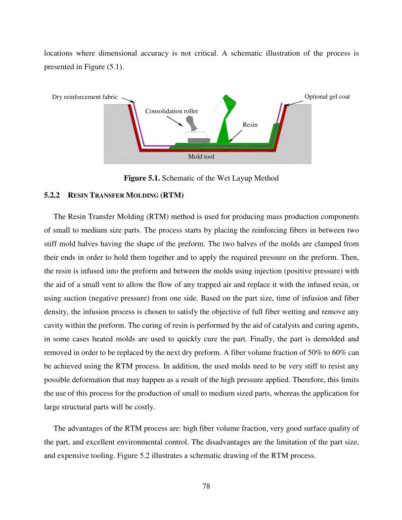
78
locations where dimensional accuracy is not critical. A schematic illustration of the process is
presented in Figure (5.1).
5.2.2 RESIN TRANSFER MOLDING (RTM)
The Resin Transfer Molding (RTM) method is used for producing mass production components
of small to medium size parts. The process starts by placing the reinforcing fibers in between two
stiff mold halves having the shape of the preform. The two halves of the molds are clamped from
their ends in order to hold them together and to apply the required pressure on the preform. Then,
the resin is infused into the preform and between the molds using injection (positive pressure) with
the aid of a small vent to allow the flow of any trapped air and replace it with the infused resin, or
using suction (negative pressure) from one side. Based on the part size, time of infusion and fiber
density, the infusion process is chosen to satisfy the objective of full fiber wetting and remove any
cavity within the preform. The curing of resin is performed by the aid of catalysts and curing agents,
in some cases heated molds are used to quickly cure the part. Finally, the part is demolded and
removed in order to be replaced by the next dry preform. A fiber volume fraction of 50% to 60% can
be achieved using the RTM process. In addition, the used molds need to be very stiff to resist any
possible deformation that may happen as a result of the high pressure applied. Therefore, this limits
the use of this process for the production of small to medium sized parts, whereas the application for
large structural parts will be costly.
The advantages of the RTM process are: high fiber volume fraction, very good surface quality of
the part, and excellent environmental control. The disadvantages are the limitation of the part size,
and expensive tooling. Figure 5.2 illustrates a schematic drawing of the RTM process.
Figure 5.1. Schematic of the Wet Layup Method
Dry reinforcement fabric
Consolidation roller
Optional gel coat
Resin
Mold tool
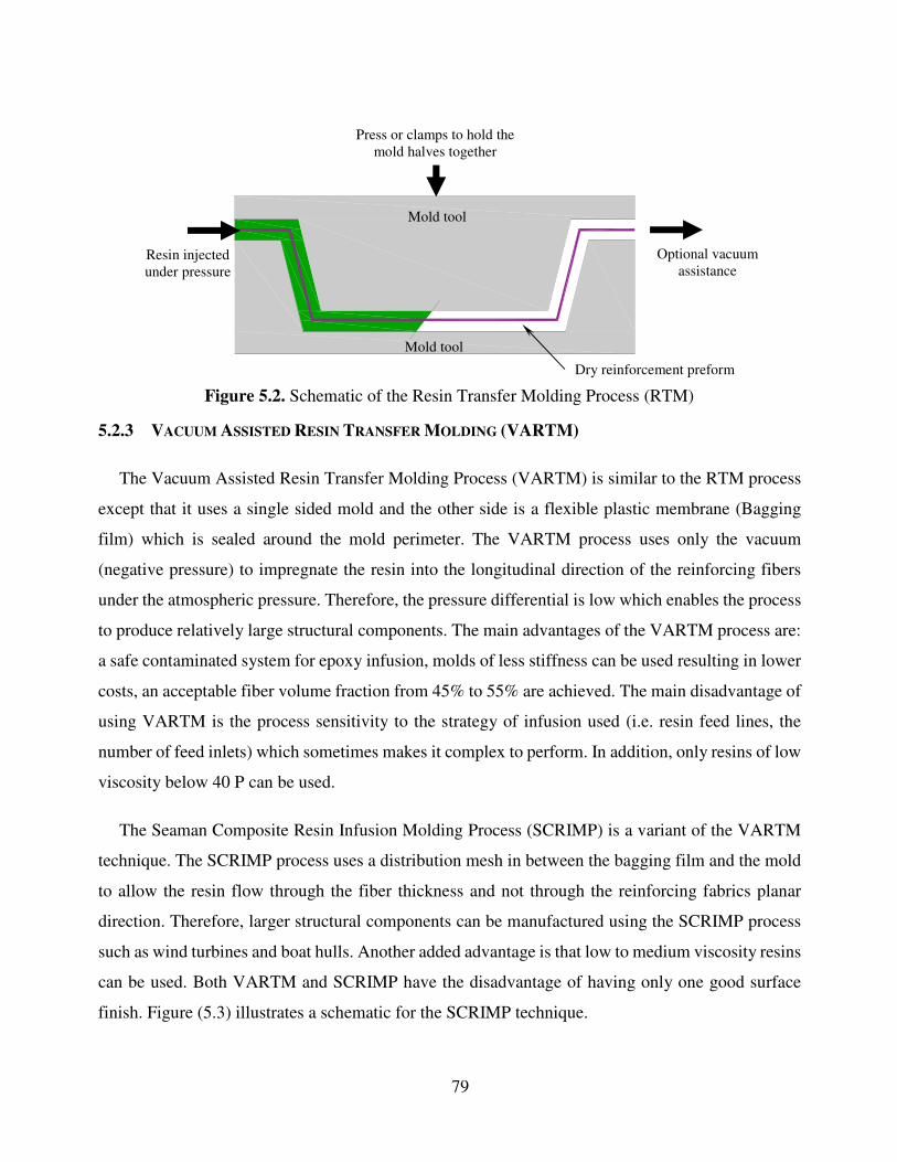
79
5.2.3 VACUUM ASSISTED RESIN TRANSFER MOLDING (VARTM)
The Vacuum Assisted Resin Transfer Molding Process (VARTM) is similar to the RTM process
except that it uses a single sided mold and the other side is a flexible plastic membrane (Bagging
film) which is sealed around the mold perimeter. The VARTM process uses only the vacuum
(negative pressure) to impregnate the resin into the longitudinal direction of the reinforcing fibers
under the atmospheric pressure. Therefore, the pressure differential is low which enables the process
to produce relatively large structural components. The main advantages of the VARTM process are:
a safe contaminated system for epoxy infusion, molds of less stiffness can be used resulting in lower
costs, an acceptable fiber volume fraction from 45% to 55% are achieved. The main disadvantage of
using VARTM is the process sensitivity to the strategy of infusion used (i.e. resin feed lines, the
number of feed inlets) which sometimes makes it complex to perform. In addition, only resins of low
viscosity below 40 P can be used.
The Seaman Composite Resin Infusion Molding Process (SCRIMP) is a variant of the VARTM
technique. The SCRIMP process uses a distribution mesh in between the bagging film and the mold
to allow the resin flow through the fiber thickness and not through the reinforcing fabrics planar
direction. Therefore, larger structural components can be manufactured using the SCRIMP process
such as wind turbines and boat hulls. Another added advantage is that low to medium viscosity resins
can be used. Both VARTM and SCRIMP have the disadvantage of having only one good surface
finish. Figure (5.3) illustrates a schematic for the SCRIMP technique.
Figure 5.2. Schematic of the Resin Transfer Molding Process (RTM)
Mold tool
Optional vacuum assistance
Mold tool
Resin injected under pressure
Press or clamps to hold the mold halves together
Dry reinforcement preform
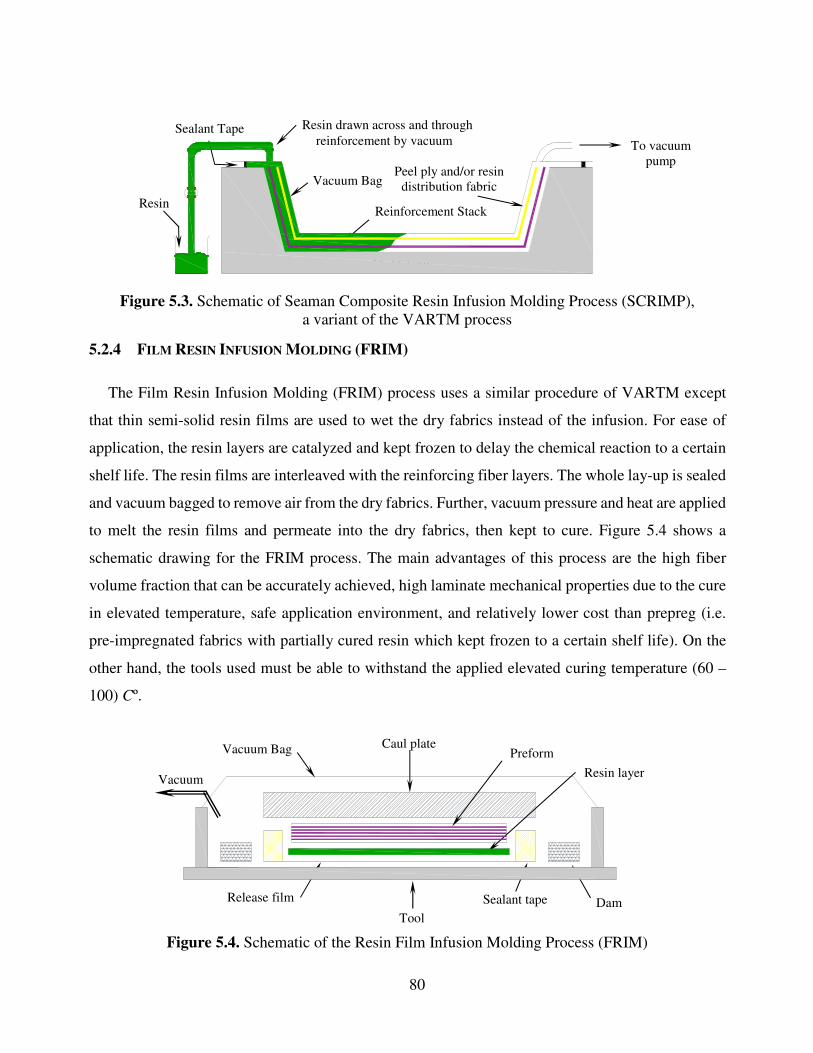
80
5.2.4 FILM RESIN INFUSION MOLDING (FRIM)
The Film Resin Infusion Molding (FRIM) process uses a similar procedure of VARTM except
that thin semi-solid resin films are used to wet the dry fabrics instead of the infusion. For ease of
application, the resin layers are catalyzed and kept frozen to delay the chemical reaction to a certain
shelf life. The resin films are interleaved with the reinforcing fiber layers. The whole lay-up is sealed
and vacuum bagged to remove air from the dry fabrics. Further, vacuum pressure and heat are applied
to melt the resin films and permeate into the dry fabrics, then kept to cure. Figure 5.4 shows a
schematic drawing for the FRIM process. The main advantages of this process are the high fiber
volume fraction that can be accurately achieved, high laminate mechanical properties due to the cure
in elevated temperature, safe application environment, and relatively lower cost than prepreg (i.e.
pre-impregnated fabrics with partially cured resin which kept frozen to a certain shelf life). On the
other hand, the tools used must be able to withstand the applied elevated curing temperature (60 –
100) Cº.
Figure 5.3. Schematic of Seaman Composite Resin Infusion Molding Process (SCRIMP), a variant of the VARTM process
Figure 5.4. Schematic of the Resin Film Infusion Molding Process (FRIM)
Mold Tool
To vacuum pump
Sealant Tape
Resin
Resin drawn across and through reinforcement by vacuum
Vacuum Bag Peel ply and/or resin
distribution fabric
Reinforcement Stack
Vacuum
Caul plate Preform
Resin layer
Release film Sealant tape Dam Tool
Vacuum Bag
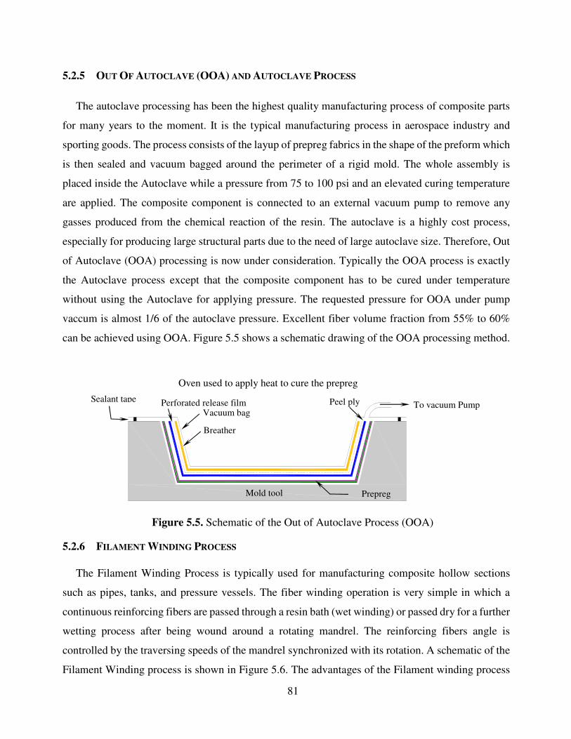
81
5.2.5 OUT OF AUTOCLAVE (OOA) AND AUTOCLAVE PROCESS
The autoclave processing has been the highest quality manufacturing process of composite parts
for many years to the moment. It is the typical manufacturing process in aerospace industry and
sporting goods. The process consists of the layup of prepreg fabrics in the shape of the preform which
is then sealed and vacuum bagged around the perimeter of a rigid mold. The whole assembly is
placed inside the Autoclave while a pressure from 75 to 100 psi and an elevated curing temperature
are applied. The composite component is connected to an external vacuum pump to remove any
gasses produced from the chemical reaction of the resin. The autoclave is a highly cost process,
especially for producing large structural parts due to the need of large autoclave size. Therefore, Out
of Autoclave (OOA) processing is now under consideration. Typically the OOA process is exactly
the Autoclave process except that the composite component has to be cured under temperature
without using the Autoclave for applying pressure. The requested pressure for OOA under pump
vaccum is almost 1/6 of the autoclave pressure. Excellent fiber volume fraction from 55% to 60%
can be achieved using OOA. Figure 5.5 shows a schematic drawing of the OOA processing method.
5.2.6 FILAMENT WINDING PROCESS
The Filament Winding Process is typically used for manufacturing composite hollow sections
such as pipes, tanks, and pressure vessels. The fiber winding operation is very simple in which a
continuous reinforcing fibers are passed through a resin bath (wet winding) or passed dry for a further
wetting process after being wound around a rotating mandrel. The reinforcing fibers angle is
controlled by the traversing speeds of the mandrel synchronized with its rotation. A schematic of the
Filament Winding process is shown in Figure 5.6. The advantages of the Filament winding process
Figure 5.5. Schematic of the Out of Autoclave Process (OOA)
Mold tool
Oven used to apply heat to cure the prepreg
Sealant tape To vacuum Pump Perforated release film
Vacuum bag
Breather
Peel ply
Prepreg
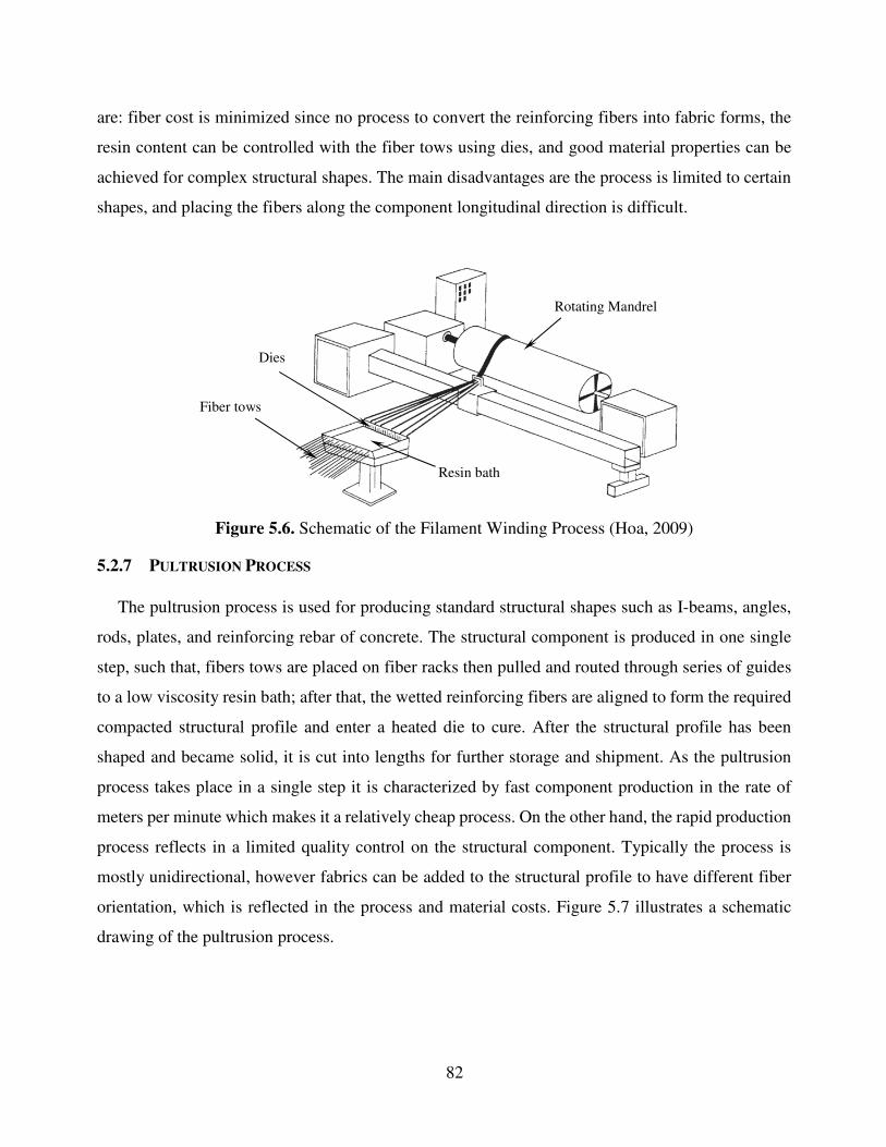
82
are: fiber cost is minimized since no process to convert the reinforcing fibers into fabric forms, the
resin content can be controlled with the fiber tows using dies, and good material properties can be
achieved for complex structural shapes. The main disadvantages are the process is limited to certain
shapes, and placing the fibers along the component longitudinal direction is difficult.
5.2.7 PULTRUSION PROCESS
The pultrusion process is used for producing standard structural shapes such as I-beams, angles,
rods, plates, and reinforcing rebar of concrete. The structural component is produced in one single
step, such that, fibers tows are placed on fiber racks then pulled and routed through series of guides
to a low viscosity resin bath; after that, the wetted reinforcing fibers are aligned to form the required
compacted structural profile and enter a heated die to cure. After the structural profile has been
shaped and became solid, it is cut into lengths for further storage and shipment. As the pultrusion
process takes place in a single step it is characterized by fast component production in the rate of
meters per minute which makes it a relatively cheap process. On the other hand, the rapid production
process reflects in a limited quality control on the structural component. Typically the process is
mostly unidirectional, however fabrics can be added to the structural profile to have different fiber
orientation, which is reflected in the process and material costs. Figure 5.7 illustrates a schematic
drawing of the pultrusion process.
Figure 5.6. Schematic of the Filament Winding Process (Hoa, 2009)
Rotating Mandrel
Fiber tows
Dies
Resin bath
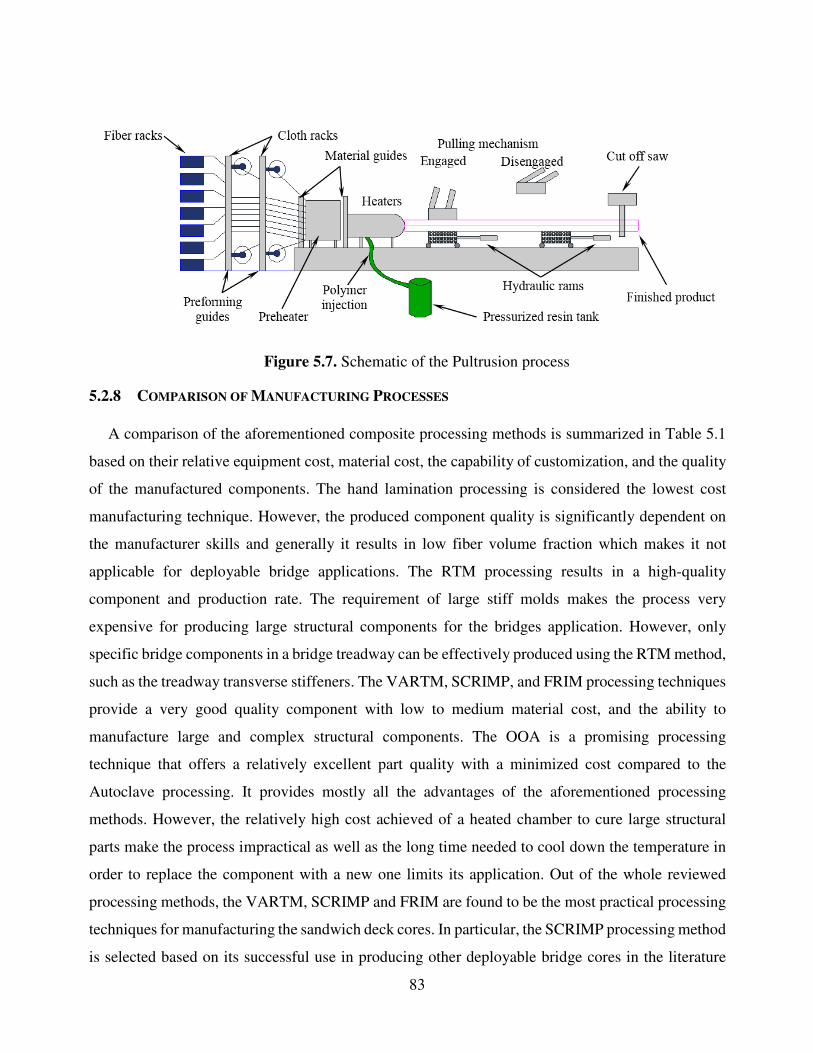
83
5.2.8 COMPARISON OF MANUFACTURING PROCESSES
A comparison of the aforementioned composite processing methods is summarized in Table 5.1
based on their relative equipment cost, material cost, the capability of customization, and the quality
of the manufactured components. The hand lamination processing is considered the lowest cost
manufacturing technique. However, the produced component quality is significantly dependent on
the manufacturer skills and generally it results in low fiber volume fraction which makes it not
applicable for deployable bridge applications. The RTM processing results in a high-quality
component and production rate. The requirement of large stiff molds makes the process very
expensive for producing large structural components for the bridges application. However, only
specific bridge components in a bridge treadway can be effectively produced using the RTM method,
such as the treadway transverse stiffeners. The VARTM, SCRIMP, and FRIM processing techniques
provide a very good quality component with low to medium material cost, and the ability to
manufacture large and complex structural components. The OOA is a promising processing
technique that offers a relatively excellent part quality with a minimized cost compared to the
Autoclave processing. It provides mostly all the advantages of the aforementioned processing
methods. However, the relatively high cost achieved of a heated chamber to cure large structural
parts make the process impractical as well as the long time needed to cool down the temperature in
order to replace the component with a new one limits its application. Out of the whole reviewed
processing methods, the VARTM, SCRIMP and FRIM are found to be the most practical processing
techniques for manufacturing the sandwich deck cores. In particular, the SCRIMP processing method
is selected based on its successful use in producing other deployable bridge cores in the literature
Figure 5.7. Schematic of the Pultrusion process
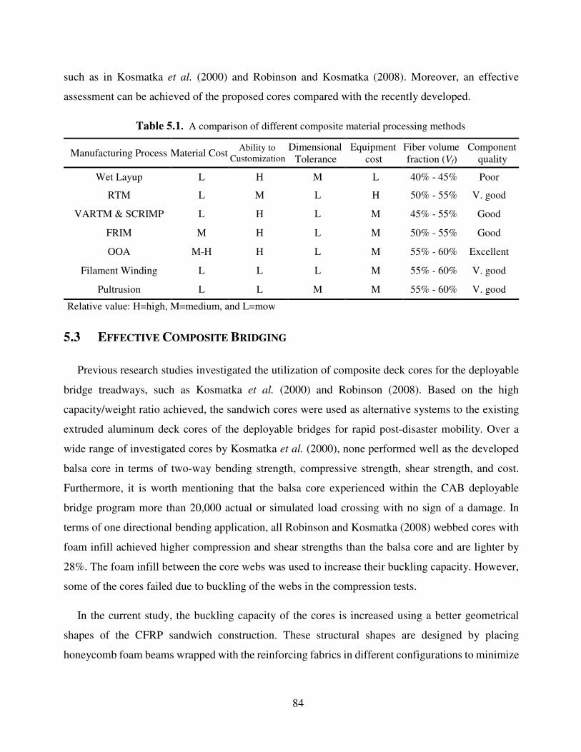
84
such as in Kosmatka et al. (2000) and Robinson and Kosmatka (2008). Moreover, an effective
assessment can be achieved of the proposed cores compared with the recently developed.
Table 5.1. A comparison of different composite material processing methods
Manufacturing Process Material Cost Ability to Customization
Dimensional Tolerance
Equipment cost
Fiber volume fraction (Vf)
Component quality
Wet Layup L H M L 40% - 45% Poor
RTM L M L H 50% - 55% V. good
VARTM & SCRIMP L H L M 45% - 55% Good
FRIM M H L M 50% - 55% Good
OOA M-H H L M 55% - 60% Excellent
Filament Winding L L L M 55% - 60% V. good
Pultrusion L L M M 55% - 60% V. good
Relative value: H=high, M=medium, and L=mow
5.3 EFFECTIVE COMPOSITE BRIDGING
Previous research studies investigated the utilization of composite deck cores for the deployable
bridge treadways, such as Kosmatka et al. (2000) and Robinson (2008). Based on the high
capacity/weight ratio achieved, the sandwich cores were used as alternative systems to the existing
extruded aluminum deck cores of the deployable bridges for rapid post-disaster mobility. Over a
wide range of investigated cores by Kosmatka et al. (2000), none performed well as the developed
balsa core in terms of two-way bending strength, compressive strength, shear strength, and cost.
Furthermore, it is worth mentioning that the balsa core experienced within the CAB deployable
bridge program more than 20,000 actual or simulated load crossing with no sign of a damage. In
terms of one directional bending application, all Robinson and Kosmatka (2008) webbed cores with
foam infill achieved higher compression and shear strengths than the balsa core and are lighter by
28%. The foam infill between the core webs was used to increase their buckling capacity. However,
some of the cores failed due to buckling of the webs in the compression tests.
In the current study, the buckling capacity of the cores is increased using a better geometrical
shapes of the CFRP sandwich construction. These structural shapes are designed by placing
honeycomb foam beams wrapped with the reinforcing fabrics in different configurations to minimize
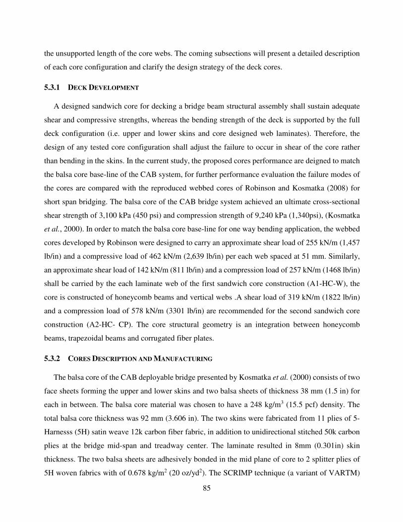
85
the unsupported length of the core webs. The coming subsections will present a detailed description
of each core configuration and clarify the design strategy of the deck cores.
5.3.1 DECK DEVELOPMENT
A designed sandwich core for decking a bridge beam structural assembly shall sustain adequate
shear and compressive strengths, whereas the bending strength of the deck is supported by the full
deck configuration (i.e. upper and lower skins and core designed web laminates). Therefore, the
design of any tested core configuration shall adjust the failure to occur in shear of the core rather
than bending in the skins. In the current study, the proposed cores performance are deigned to match
the balsa core base-line of the CAB system, for further performance evaluation the failure modes of
the cores are compared with the reproduced webbed cores of Robinson and Kosmatka (2008) for
short span bridging. The balsa core of the CAB bridge system achieved an ultimate cross-sectional
shear strength of 3,100 kPa (450 psi) and compression strength of 9,240 kPa (1,340psi), (Kosmatka
et al., 2000). In order to match the balsa core base-line for one way bending application, the webbed
cores developed by Robinson were designed to carry an approximate shear load of 255 kN/m (1,457
lb/in) and a compressive load of 462 kN/m (2,639 lb/in) per each web spaced at 51 mm. Similarly,
an approximate shear load of 142 kN/m (811 lb/in) and a compression load of 257 kN/m (1468 lb/in)
shall be carried by the each laminate web of the first sandwich core construction (A1-HC-W), the
core is constructed of honeycomb beams and vertical webs .A shear load of 319 kN/m (1822 lb/in)
and a compression load of 578 kN/m (3301 lb/in) are recommended for the second sandwich core
construction (A2-HC- CP). The core structural geometry is an integration between honeycomb
beams, trapezoidal beams and corrugated fiber plates.
5.3.2 CORES DESCRIPTION AND MANUFACTURING
The balsa core of the CAB deployable bridge presented by Kosmatka et al. (2000) consists of two
face sheets forming the upper and lower skins and two balsa sheets of thickness 38 mm (1.5 in) for
each in between. The balsa core material was chosen to have a 248 kg/m3 (15.5 pcf) density. The
total balsa core thickness was 92 mm (3.606 in). The two skins were fabricated from 11 plies of 5-
Harnesss (5H) satin weave 12k carbon fiber fabric, in addition to unidirectional stitched 50k carbon
plies at the bridge mid-span and treadway center. The laminate resulted in 8mm (0.301in) skin
thickness. The two balsa sheets are adhesively bonded in the mid plane of core to 2 splitter plies of
5H woven fabrics with of 0.678 kg/m2 (20 oz/yd2). The SCRIMP technique (a variant of VARTM)
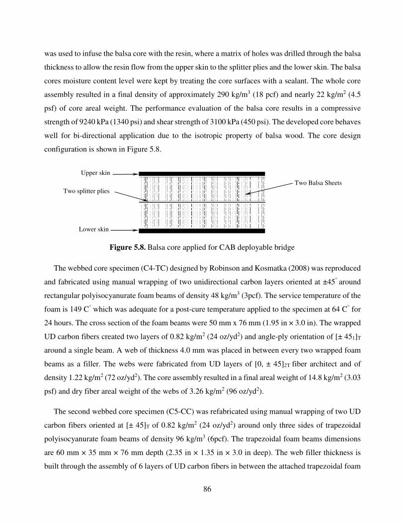
86
was used to infuse the balsa core with the resin, where a matrix of holes was drilled through the balsa
thickness to allow the resin flow from the upper skin to the splitter plies and the lower skin. The balsa
cores moisture content level were kept by treating the core surfaces with a sealant. The whole core
assembly resulted in a final density of approximately 290 kg/m3 (18 pcf) and nearly 22 kg/m2 (4.5
psf) of core areal weight. The performance evaluation of the balsa core results in a compressive
strength of 9240 kPa (1340 psi) and shear strength of 3100 kPa (450 psi). The developed core behaves
well for bi-directional application due to the isotropic property of balsa wood. The core design
configuration is shown in Figure 5.8.
Figure 5.8. Balsa core applied for CAB deployable bridge
The webbed core specimen (C4-TC) designed by Robinson and Kosmatka (2008) was reproduced
and fabricated using manual wrapping of two unidirectional carbon layers oriented at ±45° around
rectangular polyisocyanurate foam beams of density 48 kg/m3 (3pcf). The service temperature of the
foam is 149 C° which was adequate for a post-cure temperature applied to the specimen at 64 C° for
24 hours. The cross section of the foam beams were 50 mm x 76 mm (1.95 in × 3.0 in). The wrapped
UD carbon fibers created two layers of 0.82 kg/m2 (24 oz/yd2) and angle-ply orientation of [± 451]T
around a single beam. A web of thickness 4.0 mm was placed in between every two wrapped foam
beams as a filler. The webs were fabricated from UD layers of [0, ± 45]2T fiber architect and of
density 1.22 kg/m2 (72 oz/yd2). The core assembly resulted in a final areal weight of 14.8 kg/m2 (3.03
psf) and dry fiber areal weight of the webs of 3.26 kg/m2 (96 oz/yd2).
The second webbed core specimen (C5-CC) was refabricated using manual wrapping of two UD
carbon fibers oriented at [± 45]T of 0.82 kg/m2 (24 oz/yd2) around only three sides of trapezoidal
polyisocyanurate foam beams of density 96 kg/m3 (6pcf). The trapezoidal foam beams dimensions
are 60 mm × 35 mm × 76 mm depth (2.35 in × 1.35 in × 3.0 in deep). The web filler thickness is
built through the assembly of 6 layers of UD carbon fibers in between the attached trapezoidal foam
Two Balsa Sheets Two splitter plies
Upper skin
Lower skin
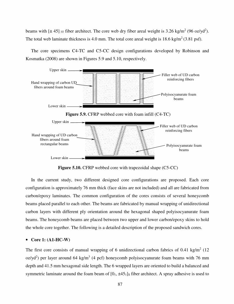
87
beams with [± 45] 3T fiber architect. The core web dry fiber areal weight is 3.26 kg/m2 (96 oz/yd2).
The total web laminate thickness is 4.0 mm. The total core areal weight is 18.6 kg/m2 (3.81 psf).
The core specimens C4-TC and C5-CC design configurations developed by Robinson and
Kosmatka (2008) are shown in Figures 5.9 and 5.10, respectively.
Figure 5.9. CFRP webbed core with foam infill (C4-TC)
Figure 5.10. CFRP webbed core with trapezoidal shape (C5-CC)
In the current study, two different designed core configurations are proposed. Each core
configuration is approximately 76 mm thick (face skins are not included) and all are fabricated from
carbon/epoxy laminates. The common configuration of the cores consists of several honeycomb
beams placed parallel to each other. The beams are fabricated by manual wrapping of unidirectional
carbon layers with different ply orientation around the hexagonal shaped polyisocyanurate foam
beams. The honeycomb beams are placed between two upper and lower carbon/epoxy skins to hold
the whole core together. The following is a detailed description of the proposed sandwich cores.
• Core 1: (A1-HC-W)
The first core consists of manual wrapping of 6 unidirectional carbon fabrics of 0.41 kg/m2 (12
oz/yd2) per layer around 64 kg/m3 (4 pcf) honeycomb polyisocyanurate foam beams with 76 mm
depth and 41.5 mm hexagonal side length. The 6 wrapped layers are oriented to build a balanced and
symmetric laminate around the foam beam of [01, ±451]S fiber architect. A spray adhesive is used to
Upper skin
Lower skin
Filler web of UD carbon reinforcing fibers
Polyisocyanurate foam beams
Hand wrapping of carbon UD fibers around foam beams
Upper skin
Lower skin
Filler web of UD carbon reinforcing fibers
Polyisocyanurate foam beams
Hand wrapping of UD carbon fibers around foam rectangular beams
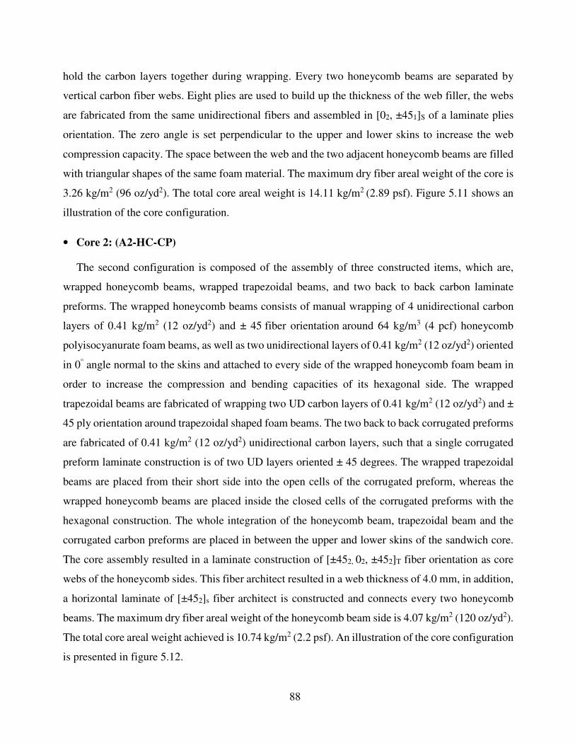
88
hold the carbon layers together during wrapping. Every two honeycomb beams are separated by
vertical carbon fiber webs. Eight plies are used to build up the thickness of the web filler, the webs
are fabricated from the same unidirectional fibers and assembled in [02, ±451]S of a laminate plies
orientation. The zero angle is set perpendicular to the upper and lower skins to increase the web
compression capacity. The space between the web and the two adjacent honeycomb beams are filled
with triangular shapes of the same foam material. The maximum dry fiber areal weight of the core is
3.26 kg/m2 (96 oz/yd2). The total core areal weight is 14.11 kg/m2 (2.89 psf). Figure 5.11 shows an
illustration of the core configuration.
• Core 2: (A2-HC-CP)
The second configuration is composed of the assembly of three constructed items, which are,
wrapped honeycomb beams, wrapped trapezoidal beams, and two back to back carbon laminate
preforms. The wrapped honeycomb beams consists of manual wrapping of 4 unidirectional carbon
layers of 0.41 kg/m2 (12 oz/yd2) and ± 45 fiber orientation around 64 kg/m3 (4 pcf) honeycomb
polyisocyanurate foam beams, as well as two unidirectional layers of 0.41 kg/m2 (12 oz/yd2) oriented
in 0° angle normal to the skins and attached to every side of the wrapped honeycomb foam beam in
order to increase the compression and bending capacities of its hexagonal side. The wrapped
trapezoidal beams are fabricated of wrapping two UD carbon layers of 0.41 kg/m2 (12 oz/yd2) and ±
45 ply orientation around trapezoidal shaped foam beams. The two back to back corrugated preforms
are fabricated of 0.41 kg/m2 (12 oz/yd2) unidirectional carbon layers, such that a single corrugated
preform laminate construction is of two UD layers oriented ± 45 degrees. The wrapped trapezoidal
beams are placed from their short side into the open cells of the corrugated preform, whereas the
wrapped honeycomb beams are placed inside the closed cells of the corrugated preforms with the
hexagonal construction. The whole integration of the honeycomb beam, trapezoidal beam and the
corrugated carbon preforms are placed in between the upper and lower skins of the sandwich core.
The core assembly resulted in a laminate construction of [±452, 02, ±452]T fiber orientation as core
webs of the honeycomb sides. This fiber architect resulted in a web thickness of 4.0 mm, in addition,
a horizontal laminate of [±452]s fiber architect is constructed and connects every two honeycomb
beams. The maximum dry fiber areal weight of the honeycomb beam side is 4.07 kg/m2 (120 oz/yd2).
The total core areal weight achieved is 10.74 kg/m2 (2.2 psf). An illustration of the core configuration
is presented in figure 5.12.
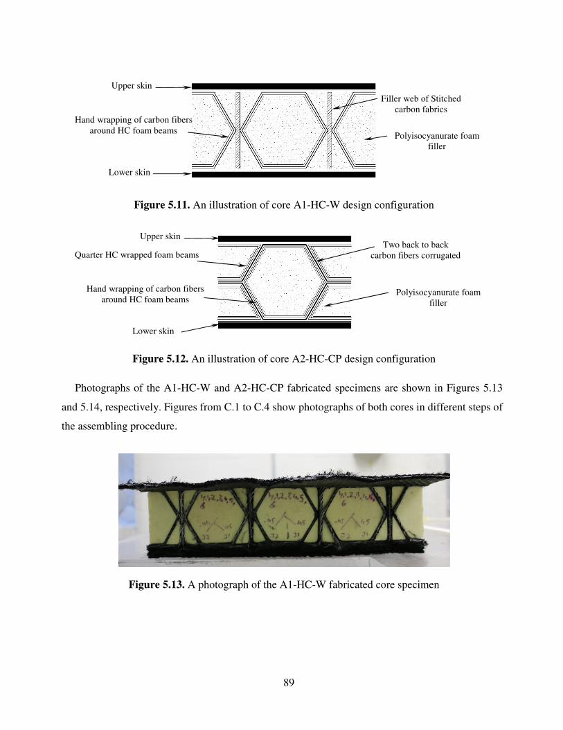
89
Figure 5.11. An illustration of core A1-HC-W design configuration
Figure 5.12. An illustration of core A2-HC-CP design configuration
Photographs of the A1-HC-W and A2-HC-CP fabricated specimens are shown in Figures 5.13
and 5.14, respectively. Figures from C.1 to C.4 show photographs of both cores in different steps of
the assembling procedure.
Figure 5.13. A photograph of the A1-HC-W fabricated core specimen
Upper skin
Lower skin
Polyisocyanurate foam filler
Two back to back carbon fibers corrugated
sheets
Hand wrapping of carbon fibers around HC foam beams
Quarter HC wrapped foam beams
Upper skin
Lower skin
Hand wrapping of carbon fibers around HC foam beams
Filler web of Stitched carbon fabrics
Polyisocyanurate foam filler
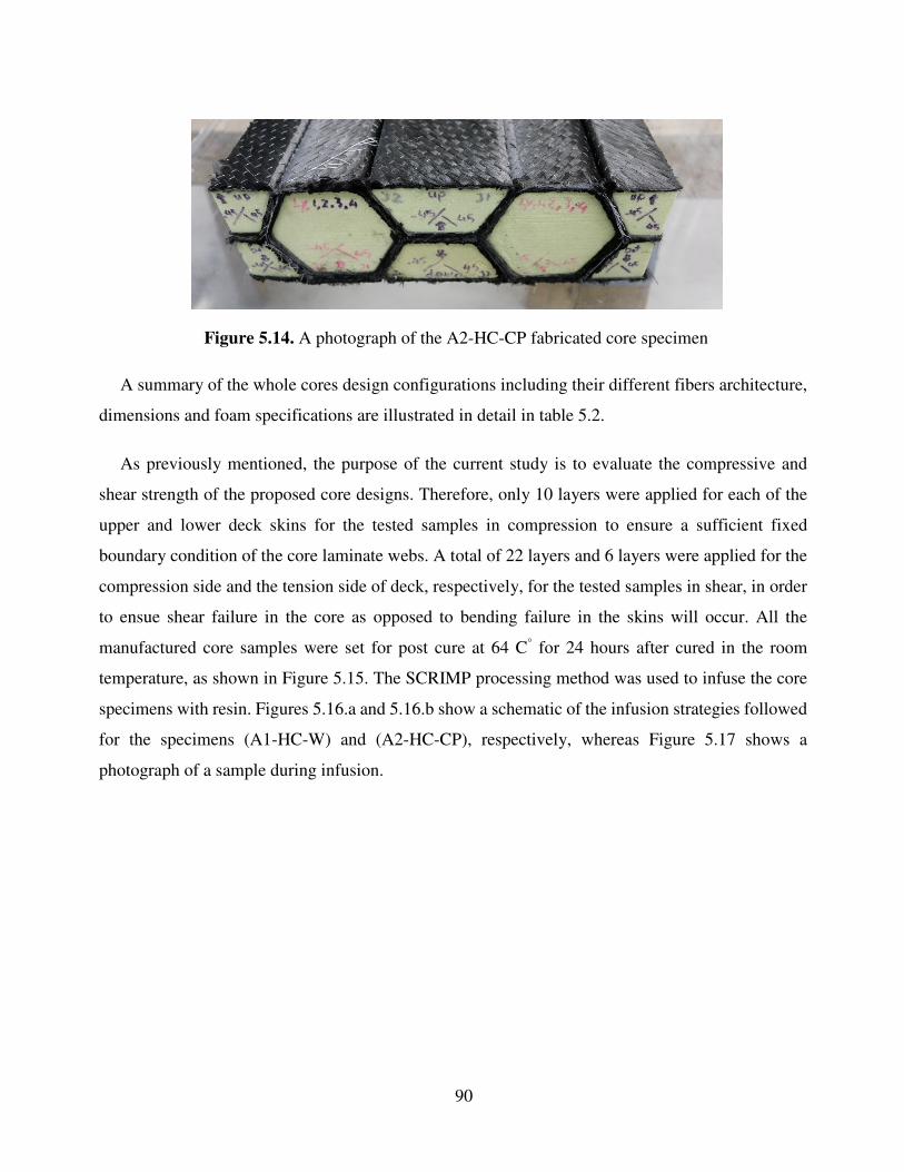
90
Figure 5.14. A photograph of the A2-HC-CP fabricated core specimen
A summary of the whole cores design configurations including their different fibers architecture,
dimensions and foam specifications are illustrated in detail in table 5.2.
As previously mentioned, the purpose of the current study is to evaluate the compressive and
shear strength of the proposed core designs. Therefore, only 10 layers were applied for each of the
upper and lower deck skins for the tested samples in compression to ensure a sufficient fixed
boundary condition of the core laminate webs. A total of 22 layers and 6 layers were applied for the
compression side and the tension side of deck, respectively, for the tested samples in shear, in order
to ensue shear failure in the core as opposed to bending failure in the skins will occur. All the
manufactured core samples were set for post cure at 64 C° for 24 hours after cured in the room
temperature, as shown in Figure 5.15. The SCRIMP processing method was used to infuse the core
specimens with resin. Figures 5.16.a and 5.16.b show a schematic of the infusion strategies followed
for the specimens (A1-HC-W) and (A2-HC-CP), respectively, whereas Figure 5.17 shows a
photograph of a sample during infusion.

91
Figure 5.15. A photograph of the A1-HC-W being post cured in Autoclave
Figure 5.16. A schematic of the infusion strategy used for the core specimens
Resin Feed Resin Feed
To catch pot and vacuum pump
Resin feed channel
Resin Distribution Media
Resin feed channel
Resin Distribution Media
To catch pot and vacuum pump
Vacuum line (spiral tube)
Vacuum line (spiral
tube)
Vacuum line (spiral
tube)
To catch pot and vacuum pump
Vacuum tight seal
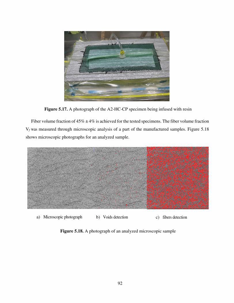
92
Figure 5.17. A photograph of the A2-HC-CP specimen being infused with resin
Fiber volume fraction of 45% ± 4% is achieved for the tested specimens. The fiber volume fraction
Vf was measured through microscopic analysis of a part of the manufactured samples. Figure 5.18
shows microscopic photographs for an analyzed sample.
a) Microscopic photograph b) Voids detection c) fibers detection
Figure 5.18. A photograph of an analyzed microscopic sample
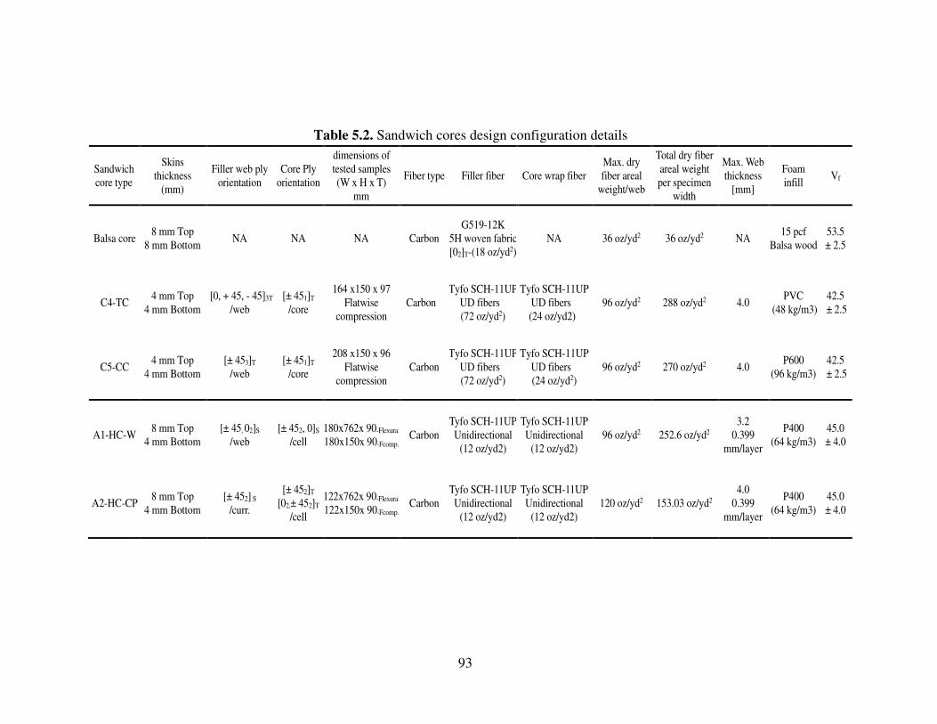
93
Table 5.2. Sandwich cores design configuration details
Sandwich core type
Skins thickness
(mm)
Filler web ply orientation
Core Ply orientation
dimensions of tested samples (W x H x T)
mm
Fiber type Filler fiber Core wrap fiber Max. dry fiber areal
weight/web
Total dry fiber areal weight per specimen
width
Max. Web thickness
[mm]
Foam infill
Vf
Balsa core 8 mm Top
8 mm Bottom NA NA NA Carbon
G519-12K 5H woven fabric [02]T-(18 oz/yd2)
NA 36 oz/yd2 36 oz/yd2 NA 15 pcf
Balsa wood 53.5 ± 2.5
C4-TC 4 mm Top
4 mm Bottom [0, + 45, - 45]3T
/web [± 451]T
/core
164 x150 x 97 Flatwise
compression Carbon
Tyfo SCH-11UPUD fibers (72 oz/yd2)
Tyfo SCH-11UP UD fibers
(24 oz/yd2) 96 oz/yd2 288 oz/yd2 4.0
PVC (48 kg/m3)
42.5 ± 2.5
C5-CC 4 mm Top
4 mm Bottom [± 453]T
/web [± 451]T
/core
208 x150 x 96 Flatwise
compression Carbon
Tyfo SCH-11UPUD fibers (72 oz/yd2)
Tyfo SCH-11UP UD fibers (24 oz/yd2)
96 oz/yd2 270 oz/yd2 4.0 P600
(96 kg/m3) 42.5
± 2.5
A1-HC-W 8 mm Top
4 mm Bottom [± 45, 02]S
/web [± 452, 0]S
/cell 180x762x 90-Flexural
180x150x 90-Fcomp. Carbon
Tyfo SCH-11UPUnidirectional
(12 oz/yd2)
Tyfo SCH-11UP Unidirectional
(12 oz/yd2) 96 oz/yd2 252.6 oz/yd2
3.2 0.399
mm/layer
P400 (64 kg/m3)
45.0 ± 4.0
A2-HC-CP 8 mm Top
4 mm Bottom [± 452] S
/curr.
[± 452]T [02,± 452]T
/cell
122x762x 90-Flexural
122x150x 90-Fcomp. Carbon
Tyfo SCH-11UPUnidirectional
(12 oz/yd2)
Tyfo SCH-11UP Unidirectional
(12 oz/yd2) 120 oz/yd2 153.03 oz/yd2
4.0 0.399
mm/layer
P400 (64 kg/m3)
45.0 ± 4.0
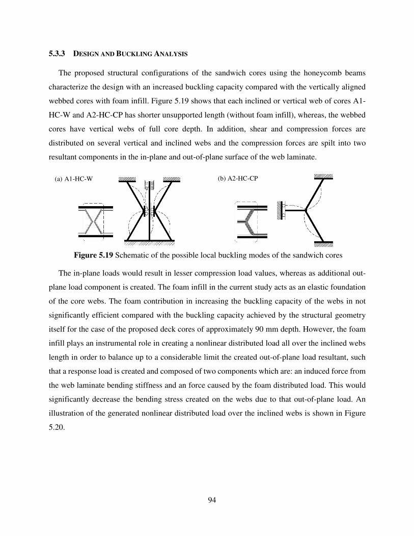
94
5.3.3 DESIGN AND BUCKLING ANALYSIS
The proposed structural configurations of the sandwich cores using the honeycomb beams
characterize the design with an increased buckling capacity compared with the vertically aligned
webbed cores with foam infill. Figure 5.19 shows that each inclined or vertical web of cores A1-
HC-W and A2-HC-CP has shorter unsupported length (without foam infill), whereas, the webbed
cores have vertical webs of full core depth. In addition, shear and compression forces are
distributed on several vertical and inclined webs and the compression forces are spilt into two
resultant components in the in-plane and out-of-plane surface of the web laminate.
Figure 5.19 Schematic of the possible local buckling modes of the sandwich cores
The in-plane loads would result in lesser compression load values, whereas as additional out-
plane load component is created. The foam infill in the current study acts as an elastic foundation
of the core webs. The foam contribution in increasing the buckling capacity of the webs in not
significantly efficient compared with the buckling capacity achieved by the structural geometry
itself for the case of the proposed deck cores of approximately 90 mm depth. However, the foam
infill plays an instrumental role in creating a nonlinear distributed load all over the inclined webs
length in order to balance up to a considerable limit the created out-of-plane load resultant, such
that a response load is created and composed of two components which are: an induced force from
the web laminate bending stiffness and an force caused by the foam distributed load. This would
significantly decrease the bending stress created on the webs due to that out-of-plane load. An
illustration of the generated nonlinear distributed load over the inclined webs is shown in Figure
5.20.
(a) A1-HC-W (b) A2-HC-CP
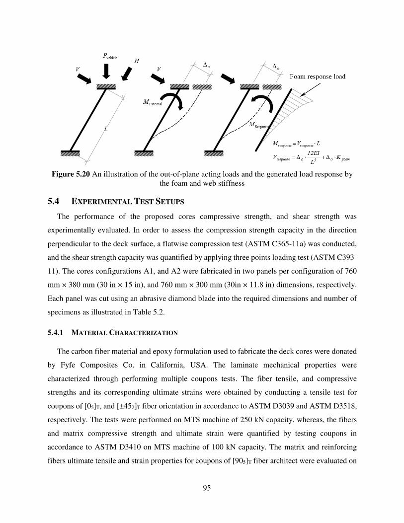
95
Figure 5.20 An illustration of the out-of-plane acting loads and the generated load response by
the foam and web stiffness
5.4 EXPERIMENTAL TEST SETUPS
The performance of the proposed cores compressive strength, and shear strength was
experimentally evaluated. In order to assess the compression strength capacity in the direction
perpendicular to the deck surface, a flatwise compression test (ASTM C365-11a) was conducted,
and the shear strength capacity was quantified by applying three points loading test (ASTM C393-
11). The cores configurations A1, and A2 were fabricated in two panels per configuration of 760
mm × 380 mm (30 in × 15 in), and 760 mm × 300 mm (30in × 11.8 in) dimensions, respectively.
Each panel was cut using an abrasive diamond blade into the required dimensions and number of
specimens as illustrated in Table 5.2.
5.4.1 MATERIAL CHARACTERIZATION
The carbon fiber material and epoxy formulation used to fabricate the deck cores were donated
by Fyfe Composites Co. in California, USA. The laminate mechanical properties were
characterized through performing multiple coupons tests. The fiber tensile, and compressive
strengths and its corresponding ultimate strains were obtained by conducting a tensile test for
coupons of [05]T, and [±452]T fiber orientation in accordance to ASTM D3039 and ASTM D3518,
respectively. The tests were performed on MTS machine of 250 kN capacity, whereas, the fibers
and matrix compressive strength and ultimate strain were quantified by testing coupons in
accordance to ASTM D3410 on MTS machine of 100 kN capacity. The matrix and reinforcing
fibers ultimate tensile and strain properties for coupons of [905]T fiber architect were evaluated on
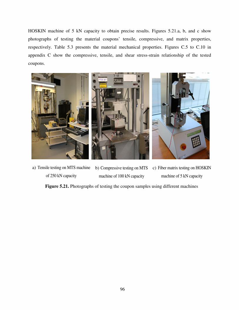
96
HOSKIN machine of 5 kN capacity to obtain precise results. Figures 5.21.a, b, and c show
photographs of testing the material coupons’ tensile, compressive, and matrix properties,
respectively. Table 5.3 presents the material mechanical properties. Figures C.5 to C.10 in
appendix C show the compressive, tensile, and shear stress-strain relationship of the tested
coupons.
a) Tensile testing on MTS machine
of 250 kN capacity
b) Compressive testing on MTS
machine of 100 kN capacity
c) Fiber matrix testing on HOSKIN
machine of 5 kN capacity
Figure 5.21. Photographs of testing the coupon samples using different machines
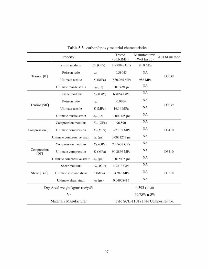
97
Table 5.3. carbon/epoxy material characteristics
Property Tested (SCRIMP)
Manufacturer (Wet layup)
ASTM method
Tension [0°]
Tensile modulus E1t (GPa) 119.0845 GPa 95.8 GPa
D3039 Poisson ratio υ12 0.38045 NA
Ultimate tensile Xt (MPa) 1580.065 MPa 986 MPa
Ultimate tensile strain ε1t (µε) 0.013691 µε NA
Tension [90°]
Tensile modulus E2t (GPa) 6.4054 GPa NA
D3039 Poisson ratio υ21 0.0204 NA
Ultimate tensile Yt (MPa) 16.14 MPa NA
Ultimate tensile strain ε2t (µε) 0.002325 µε NA
Compression [0°]
Compression modulus E1c (GPa) 96.590 NA
D3410 Ultimate compression Xc (MPa) 322.105 MPa NA
Ultimate compressive strain ε1c (µε) 0.0031273 µε NA
Compression [90°]
Compression modulus E2c (GPa) 7.45637 GPa NA
D3410 Ultimate compression Yc (MPa) 90.2869 MPa NA
Ultimate compressive strain ε2c (µε) 0.015575 µε NA
Shear [±45°]
Shear modulus G12 (GPa) 4.2813 GPa NA
D3518 Ultimate in-plane shear S (MPa) 34.916 MPa NA
Ultimate shear strain γ12 (µε) 0.04908415 NA
Dry Areal weight kg/m2 (oz/yd2) 0.393 (11.6)
Vf 46.75% ± 3%
Material / Manufacturer Tyfo SCH-11UP/ Fyfe Composites Co.
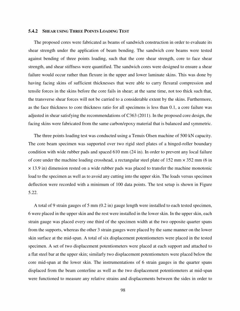
98
5.4.2 SHEAR USING THREE POINTS LOADING TEST
The proposed cores were fabricated as beams of sandwich construction in order to evaluate its
shear strength under the application of beam bending. The sandwich core beams were tested
against bending of three points loading, such that the core shear strength, core to face shear
strength, and shear stiffness were quantified. The sandwich cores were designed to ensure a shear
failure would occur rather than flexure in the upper and lower laminate skins. This was done by
having facing skins of sufficient thicknesses that were able to carry flexural compression and
tensile forces in the skins before the core fails in shear; at the same time, not too thick such that,
the transverse shear forces will not be carried to a considerable extent by the skins. Furthermore,
as the face thickness to core thickness ratio for all specimens is less than 0.1, a core failure was
adjusted in shear satisfying the recommendations of C363 (2011). In the proposed core design, the
facing skins were fabricated from the same carbon/epoxy material that is balanced and symmetric.
The three points loading test was conducted using a Tenuis Olsen machine of 500 kN capacity.
The core beam specimen was supported over two rigid steel plates of a hinged-roller boundary
condition with wide rubber pads and spaced 610 mm (24 in). In order to prevent any local failure
of core under the machine loading crosshead, a rectangular steel plate of 152 mm × 352 mm (6 in
× 13.9 in) dimension rested on a wide rubber pads was placed to transfer the machine monotonic
load to the specimen as well as to avoid any cutting into the upper skin. The loads versus specimen
deflection were recorded with a minimum of 100 data points. The test setup is shown in Figure
5.22.
A total of 9 strain gauges of 5 mm (0.2 in) gauge length were installed to each tested specimen,
6 were placed in the upper skin and the rest were installed in the lower skin. In the upper skin, each
strain gauge was placed every one third of the specimen width at the two opposite quarter spans
from the supports, whereas the other 3 strain gauges were placed by the same manner on the lower
skin surface at the mid-span. A total of six displacement potentiometers were placed in the tested
specimen. A set of two displacement potentiometers were placed at each support and attached to
a flat steel bar at the upper skin; similarly two displacement potentiometers were placed below the
core mid-span at the lower skin. The instrumentations of 6 strain gauges in the quarter spans
displaced from the beam centerline as well as the two displacement potentiometers at mid-span
were functioned to measure any relative strains and displacements between the sides in order to
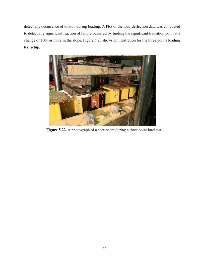
99
detect any occurrence of torsion during loading. A Plot of the load-deflection data was conducted
to detect any significant fraction of failure occurred by finding the significant transition point at a
change of 10% or more in the slope. Figure 5.23 shows an illustration for the three points loading
test setup.
Figure 5.22. A photograph of a core beam during a three point load test
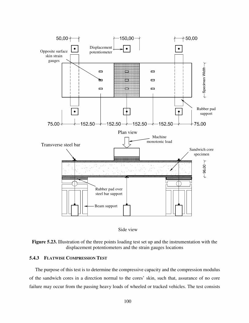
100
Figure 5.23. Illustration of the three points loading test set up and the instrumentation with the displacement potentiometers and the strain gauges locations
5.4.3 FLATWISE COMPRESSION TEST
The purpose of this test is to determine the compressive capacity and the compression modulus
of the sandwich cores in a direction normal to the cores’ skin, such that, assurance of no core
failure may occur from the passing heavy loads of wheeled or tracked vehicles. The test consists
Rubber pad support
Opposite surface skin strain
gauges
Displacement potentiometer
Machine monotonic load
Side view
Plan view
Sandwich core specimen
Rubber pad over steel bar support
Beam support
Transverse steel bar
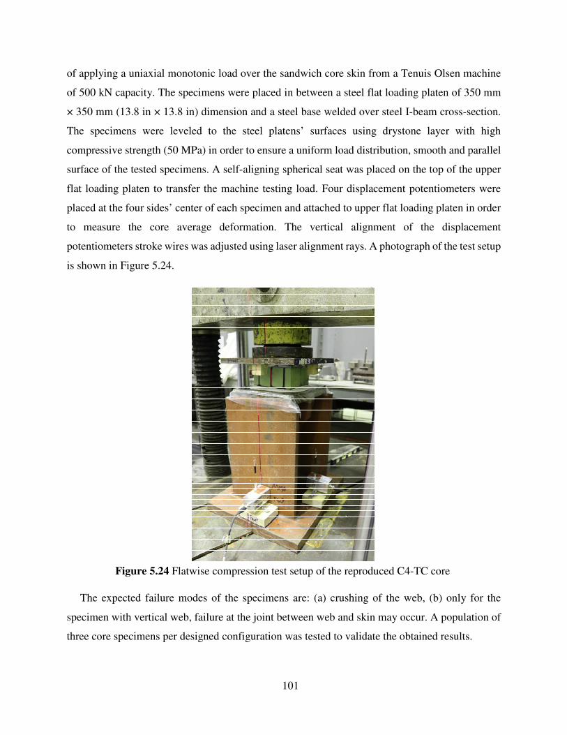
101
of applying a uniaxial monotonic load over the sandwich core skin from a Tenuis Olsen machine
of 500 kN capacity. The specimens were placed in between a steel flat loading platen of 350 mm
× 350 mm (13.8 in × 13.8 in) dimension and a steel base welded over steel I-beam cross-section.
The specimens were leveled to the steel platens’ surfaces using drystone layer with high
compressive strength (50 MPa) in order to ensure a uniform load distribution, smooth and parallel
surface of the tested specimens. A self-aligning spherical seat was placed on the top of the upper
flat loading platen to transfer the machine testing load. Four displacement potentiometers were
placed at the four sides’ center of each specimen and attached to upper flat loading platen in order
to measure the core average deformation. The vertical alignment of the displacement
potentiometers stroke wires was adjusted using laser alignment rays. A photograph of the test setup
is shown in Figure 5.24.
Figure 5.24 Flatwise compression test setup of the reproduced C4-TC core
The expected failure modes of the specimens are: (a) crushing of the web, (b) only for the
specimen with vertical web, failure at the joint between web and skin may occur. A population of
three core specimens per designed configuration was tested to validate the obtained results.
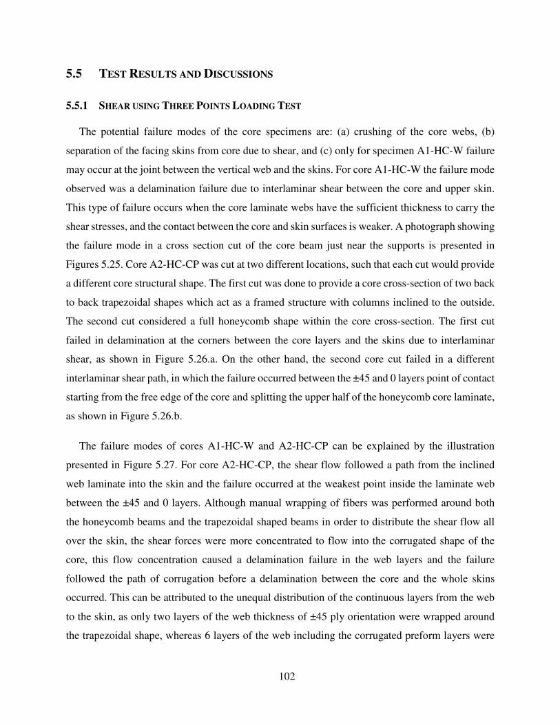
102
5.5 TEST RESULTS AND DISCUSSIONS
5.5.1 SHEAR USING THREE POINTS LOADING TEST
The potential failure modes of the core specimens are: (a) crushing of the core webs, (b)
separation of the facing skins from core due to shear, and (c) only for specimen A1-HC-W failure
may occur at the joint between the vertical web and the skins. For core A1-HC-W the failure mode
observed was a delamination failure due to interlaminar shear between the core and upper skin.
This type of failure occurs when the core laminate webs have the sufficient thickness to carry the
shear stresses, and the contact between the core and skin surfaces is weaker. A photograph showing
the failure mode in a cross section cut of the core beam just near the supports is presented in
Figures 5.25. Core A2-HC-CP was cut at two different locations, such that each cut would provide
a different core structural shape. The first cut was done to provide a core cross-section of two back
to back trapezoidal shapes which act as a framed structure with columns inclined to the outside.
The second cut considered a full honeycomb shape within the core cross-section. The first cut
failed in delamination at the corners between the core layers and the skins due to interlaminar
shear, as shown in Figure 5.26.a. On the other hand, the second core cut failed in a different
interlaminar shear path, in which the failure occurred between the ±45 and 0 layers point of contact
starting from the free edge of the core and splitting the upper half of the honeycomb core laminate,
as shown in Figure 5.26.b.
The failure modes of cores A1-HC-W and A2-HC-CP can be explained by the illustration
presented in Figure 5.27. For core A2-HC-CP, the shear flow followed a path from the inclined
web laminate into the skin and the failure occurred at the weakest point inside the laminate web
between the ±45 and 0 layers. Although manual wrapping of fibers was performed around both
the honeycomb beams and the trapezoidal shaped beams in order to distribute the shear flow all
over the skin, the shear forces were more concentrated to flow into the corrugated shape of the
core, this flow concentration caused a delamination failure in the web layers and the failure
followed the path of corrugation before a delamination between the core and the whole skins
occurred. This can be attributed to the unequal distribution of the continuous layers from the web
to the skin, as only two layers of the web thickness of ±45 ply orientation were wrapped around
the trapezoidal shape, whereas 6 layers of the web including the corrugated preform layers were
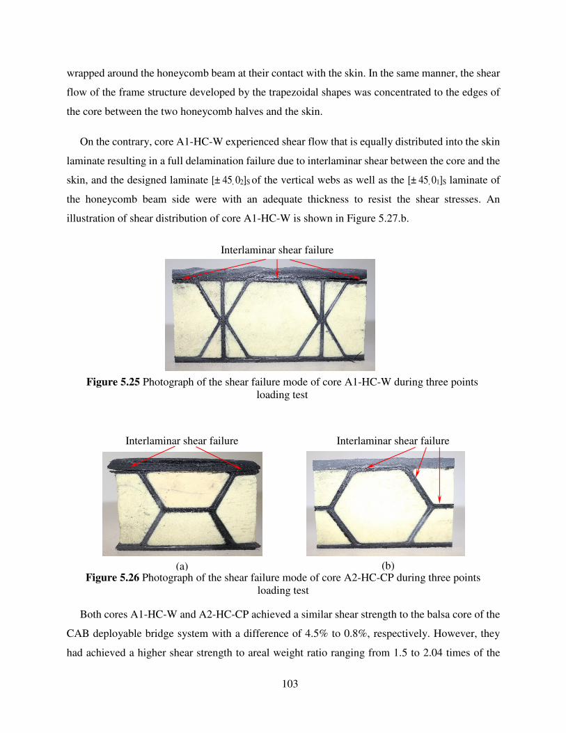
103
wrapped around the honeycomb beam at their contact with the skin. In the same manner, the shear
flow of the frame structure developed by the trapezoidal shapes was concentrated to the edges of
the core between the two honeycomb halves and the skin.
On the contrary, core A1-HC-W experienced shear flow that is equally distributed into the skin
laminate resulting in a full delamination failure due to interlaminar shear between the core and the
skin, and the designed laminate [± 45, 02]S of the vertical webs as well as the [± 45, 01]S laminate of
the honeycomb beam side were with an adequate thickness to resist the shear stresses. An
illustration of shear distribution of core A1-HC-W is shown in Figure 5.27.b.
Figure 5.25 Photograph of the shear failure mode of core A1-HC-W during three points loading test
Figure 5.26 Photograph of the shear failure mode of core A2-HC-CP during three points loading test
Both cores A1-HC-W and A2-HC-CP achieved a similar shear strength to the balsa core of the
CAB deployable bridge system with a difference of 4.5% to 0.8%, respectively. However, they
had achieved a higher shear strength to areal weight ratio ranging from 1.5 to 2.04 times of the
(a)
Interlaminar shear failure
(b)
Interlaminar shear failure
Interlaminar shear failure
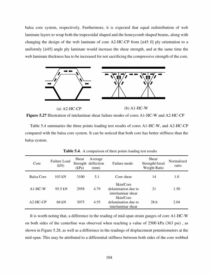
104
balsa core system, respectively. Furthermore, it is expected that equal redistribution of web
laminate layers to wrap both the trapezoidal shaped and the honeycomb shaped beams, along with
changing the design of the web laminate of core A2-HC-CP from [±45, 0] ply orientation to a
uniformly [±45] angle ply laminate would increase the shear strength, and at the same time the
web laminate thickness has to be increased for not sacrificing the compressive strength of the core.
Figure 5.27 Illustration of intelaminar shear failure modes of cores A1-HC-W and A2-HC-CP
Table 5.4 summaries the three points loading test results of cores A1-HC-W, and A2-HC-CP
compared with the balsa core system. It can be noticed that both core has better stiffness than the
balsa system.
Table 5.4. A comparison of three points loading test results
Core Failure Load
(kN)
Shear Strength
(kPa)
Average deflection
(mm) Failure mode
Shear Strength/Areal Weight Ratio
Normalized ratio
Balsa Core 103 kN 3100 5.1 Core shear 14 1.0
A1-HC-W 95.5 kN 2958 4.79 Skin/Core
delamination due to interlaminar shear
21 1.50
A2-HC-CP 68 kN 3075 4.55 Skin/Core
delamination due to interlaminar shear
28.6 2.04
It is worth noting that, a difference in the reading of mid-span strain gauges of core A1-HC-W
on both sides of the centerline was observed when reaching a value of 2500 kPa (363 psi) , as
shown in Figure 5.28, as well as a difference in the readings of displacement potentiometers at the
mid-span. This may be attributed to a differential stiffness between both sides of the core webbed
(a) A2-HC-CP (b) A1-HC-W
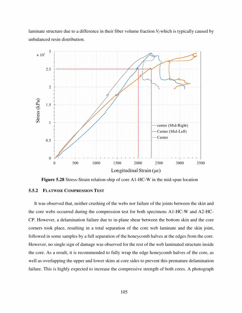
105
laminate structure due to a difference in their fiber volume fraction Vf which is typically caused by
unbalanced resin distribution.
Figure 5.28 Stress-Strain relation-ship of core A1-HC-W in the mid-span location
5.5.2 FLATWISE COMPRESSION TEST
It was observed that, neither crushing of the webs nor failure of the joints between the skin and
the core webs occurred during the compression test for both specimens A1-HC-W and A2-HC-
CP. However, a delamination failure due to in-plane shear between the bottom skin and the core
corners took place, resulting in a total separation of the core web laminate and the skin joint,
followed in some samples by a full separation of the honeycomb halves at the edges from the core.
However, no single sign of damage was observed for the rest of the web laminated structure inside
the core. As a result, it is recommended to fully wrap the edge honeycomb halves of the core, as
well as overlapping the upper and lower skins at core sides to prevent this premature delamination
failure. This is highly expected to increase the compressive strength of both cores. A photograph
× 103
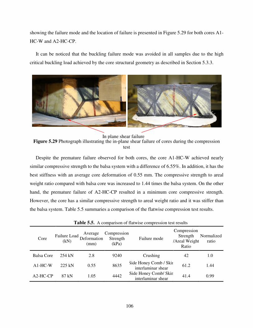
106
showing the failure mode and the location of failure is presented in Figure 5.29 for both cores A1-
HC-W and A2-HC-CP.
It can be noticed that the buckling failure mode was avoided in all samples due to the high
critical buckling load achieved by the core structural geometry as described in Section 5.3.3.
Figure 5.29 Photograph illustrating the in-plane shear failure of cores during the compression test
Despite the premature failure observed for both cores, the core A1-HC-W achieved nearly
similar compressive strength to the balsa system with a difference of 6.55%. In addition, it has the
best stiffness with an average core deformation of 0.55 mm. The compressive strength to areal
weight ratio compared with balsa core was increased to 1.44 times the balsa system. On the other
hand, the premature failure of A2-HC-CP resulted in a minimum core compressive strength.
However, the core has a similar compressive strength to areal weight ratio and it was stiffer than
the balsa system. Table 5.5 summaries a comparison of the flatwise compression test results.
Table 5.5. A comparison of flatwise compression test results
Core Failure Load
(kN)
Average Deformation
(mm)
Compression Strength
(kPa) Failure mode
Compression Strength
/Areal Weight Ratio
Normalized ratio
Balsa Core 254 kN 2.8 9240 Crushing 42 1.0
A1-HC-W 225 kN 0.55 8635 Side Honey Comb / Skin
interlaminar shear 61.2 1.44
A2-HC-CP 87 kN 1.05 4442 Side Honey Comb/ Skin
interlaminar shear 41.4 0.99
In plane shear failure
107
5.5.3 COMPARISON WITH CFRP WEBBED CORES
The cores C4-TC and C5-CC developed by Robinson and Kosmatka (2008) achieved a
compression strength of 16100 kPa (2330 psi) and 15300 kPa (2220 psi), respectively. These
values were obtained by fabricating the cores using Shell Epon 862 epoxy with Lindride 6
hardener. Due to the difficulty in obtaining the same material and epoxy formulation used by
Robinson and Kosmatka (2008) to develop all the core specimens, the webbed cores were
reproduced using the current study characterized material in order to constraint the evaluation of
cores to the deck structural shape. From a strength point of view, the web laminate thickness is
governed by the compressive strength (Robinson and Kosmatka, 2008). Therefore, only the
compression test was conducted for the webbed cores and the current study cores for re-evaluation.
Despite the premature failure occurred for cores A1-HC-W and A2-HC-CP as a result of the
delamination failure at corners as previously explained, it was found that both cores A1-HC-W
and A2-HC-CP achieved higher compressive strength than C5-CC by 2.11 and 1.08 times, and
better compressive strength to areal weight ratio by 2.78 and 1.88 times, respectively, whereas
their compressive strength was less than core C4-TC by 25.09% and 61.9%, respectively.
However, it has a more stiffness by 2.3 times than that of core C4-TC.
With respect to the design recommendation explained earlier for wrapping the honeycomb
halves at the edge of the bridge deck and overlapping the upper and lower skins on the edge sides,
the failure mode will be transformed to be either a skin/core delamination or crushing of the core
webs. Therefore, an expected higher compressive strength will be achieved for both cores, such
that the webs will be efficiently functioned to carry the compressive stresses. Based on a Classical
Lamination Theory (CLT) analytical analysis of A1-HC-W and A2-HC-CP web laminates, and
using Tsai-Wu and Maximum Stress failure theories, it is expected that core A1-HC-W is able to
resist an average compression strength obtained from the two failure theories of 18872 kPa (2737
psi), which is higher than the compression strength of core C4-TC by 1.62 times using the current
study material and resin formulation, and by 1.17 times of the result obtained by Robinson and
Kosmatka (2008). In addition, a higher compression strength to areal weight ratio of 1.21 times is
predicted compared with the result obtained by Robinson and Kosmatka (2008). The core A2-HC-
CP is expected to resist an average compressive strength of the two failure theories of 12060 kPa
(1749 psi), this value provides a similar compressive strength to areal weight ratio of core C4-TC
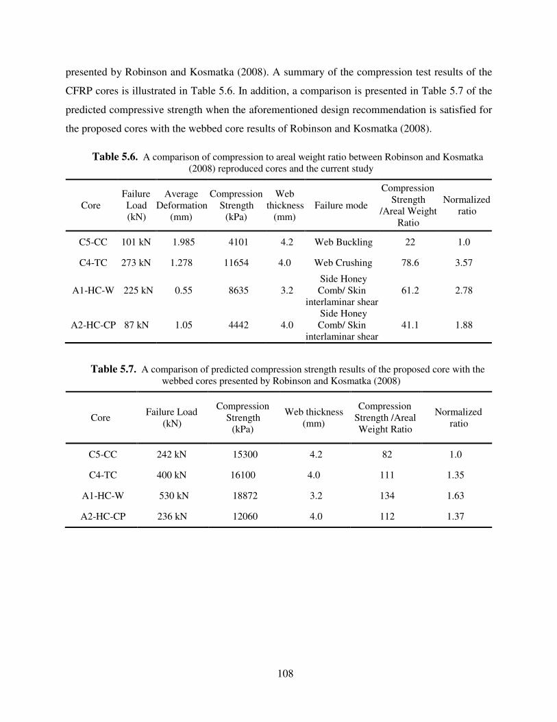
108
presented by Robinson and Kosmatka (2008). A summary of the compression test results of the
CFRP cores is illustrated in Table 5.6. In addition, a comparison is presented in Table 5.7 of the
predicted compressive strength when the aforementioned design recommendation is satisfied for
the proposed cores with the webbed core results of Robinson and Kosmatka (2008).
Table 5.6. A comparison of compression to areal weight ratio between Robinson and Kosmatka (2008) reproduced cores and the current study
Core Failure Load (kN)
Average Deformation
(mm)
Compression Strength
(kPa)
Web thickness
(mm) Failure mode
Compression Strength
/Areal Weight Ratio
Normalized ratio
C5-CC 101 kN 1.985 4101 4.2 Web Buckling 22 1.0
C4-TC 273 kN 1.278 11654 4.0 Web Crushing 78.6 3.57
A1-HC-W 225 kN 0.55 8635 3.2 Side Honey Comb/ Skin
interlaminar shear 61.2 2.78
A2-HC-CP 87 kN 1.05 4442 4.0 Side Honey Comb/ Skin
interlaminar shear 41.1 1.88
Table 5.7. A comparison of predicted compression strength results of the proposed core with the webbed cores presented by Robinson and Kosmatka (2008)
Core Failure Load
(kN)
Compression Strength
(kPa)
Web thickness (mm)
Compression Strength /Areal Weight Ratio
Normalized ratio
C5-CC 242 kN 15300 4.2 82 1.0
C4-TC 400 kN 16100 4.0 111 1.35
A1-HC-W 530 kN 18872 3.2 134 1.63
A2-HC-CP 236 kN 12060 4.0 112 1.37
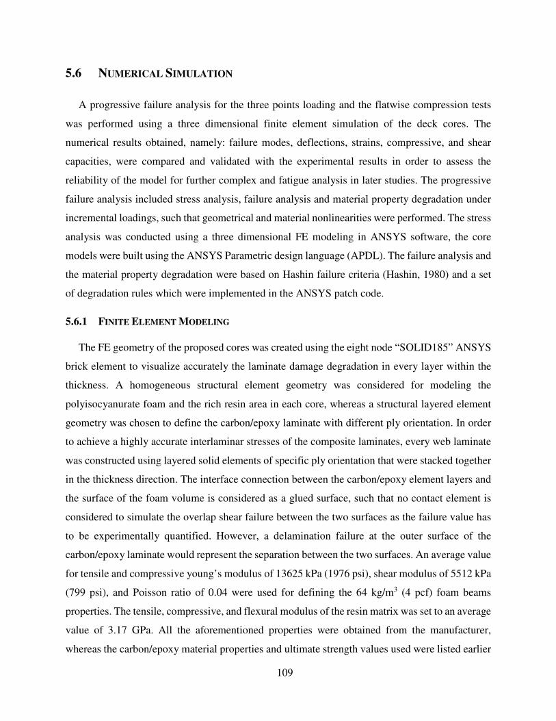
109
5.6 NUMERICAL SIMULATION
A progressive failure analysis for the three points loading and the flatwise compression tests
was performed using a three dimensional finite element simulation of the deck cores. The
numerical results obtained, namely: failure modes, deflections, strains, compressive, and shear
capacities, were compared and validated with the experimental results in order to assess the
reliability of the model for further complex and fatigue analysis in later studies. The progressive
failure analysis included stress analysis, failure analysis and material property degradation under
incremental loadings, such that geometrical and material nonlinearities were performed. The stress
analysis was conducted using a three dimensional FE modeling in ANSYS software, the core
models were built using the ANSYS Parametric design language (APDL). The failure analysis and
the material property degradation were based on Hashin failure criteria (Hashin, 1980) and a set
of degradation rules which were implemented in the ANSYS patch code.
5.6.1 FINITE ELEMENT MODELING
The FE geometry of the proposed cores was created using the eight node “SOLID185” ANSYS
brick element to visualize accurately the laminate damage degradation in every layer within the
thickness. A homogeneous structural element geometry was considered for modeling the
polyisocyanurate foam and the rich resin area in each core, whereas a structural layered element
geometry was chosen to define the carbon/epoxy laminate with different ply orientation. In order
to achieve a highly accurate interlaminar stresses of the composite laminates, every web laminate
was constructed using layered solid elements of specific ply orientation that were stacked together
in the thickness direction. The interface connection between the carbon/epoxy element layers and
the surface of the foam volume is considered as a glued surface, such that no contact element is
considered to simulate the overlap shear failure between the two surfaces as the failure value has
to be experimentally quantified. However, a delamination failure at the outer surface of the
carbon/epoxy laminate would represent the separation between the two surfaces. An average value
for tensile and compressive young’s modulus of 13625 kPa (1976 psi), shear modulus of 5512 kPa
(799 psi), and Poisson ratio of 0.04 were used for defining the 64 kg/m3 (4 pcf) foam beams
properties. The tensile, compressive, and flexural modulus of the resin matrix was set to an average
value of 3.17 GPa. All the aforementioned properties were obtained from the manufacturer,
whereas the carbon/epoxy material properties and ultimate strength values used were listed earlier
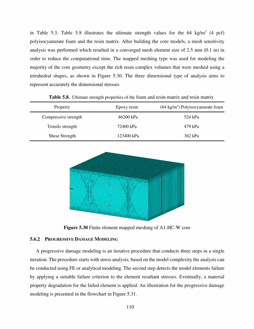
110
in Table 5.3. Table 5.8 illustrates the ultimate strength values for the 64 kg/m3 (4 pcf)
polyisocyanurate foam and the resin matrix. After building the core models, a mesh sensitivity
analysis was performed which resulted in a converged mesh element size of 2.5 mm (0.1 in) in
order to reduce the computational time. The mapped meshing type was used for modeling the
majority of the core geometry except the rich resin complex volumes that were meshed using a
tetrahedral shapes, as shown in Figure 5.30. The three dimensional type of analysis aims to
represent accurately the dimensional stresses
Table 5.8. Ultimate strength properties of the foam and resin matrix and resin matrix
Property Epoxy resin (64 kg/m3) Polyisocyanurate foam
Compressive strength 86200 kPa 524 kPa
Tensile strength 72400 kPa 479 kPa
Shear Strength 123400 kPa 362 kPa
Figure 5.30 Finite element mapped meshing of A1-HC-W core
5.6.2 PROGRESSIVE DAMAGE MODELING
A progressive damage modeling is an iterative procedure that conducts three steps in a single
iteration. The procedure starts with stress analysis, based on the model complexity the analysis can
be conducted using FE or analytical modeling. The second step detects the model elements failure
by applying a suitable failure criterion to the element resultant stresses. Eventually, a material
property degradation for the failed element is applied. An illustration for the progressive damage
modeling is presented in the flowchart in Figure 5.31.
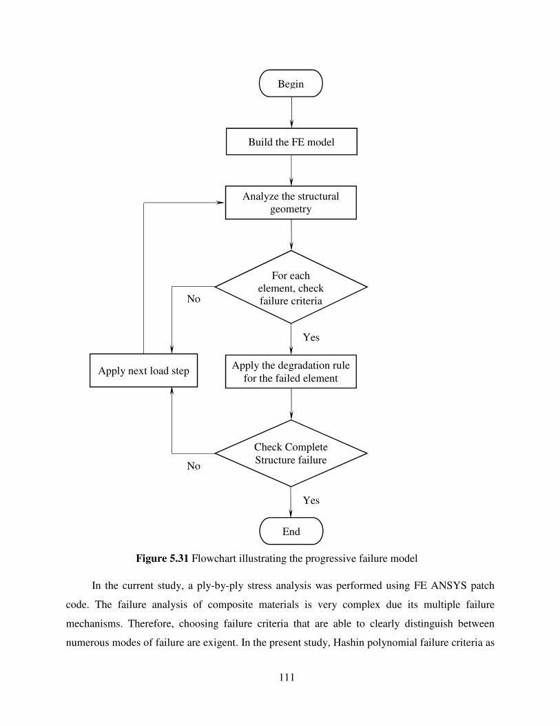
111
Figure 5.31 Flowchart illustrating the progressive failure model
In the current study, a ply-by-ply stress analysis was performed using FE ANSYS patch
code. The failure analysis of composite materials is very complex due its multiple failure
mechanisms. Therefore, choosing failure criteria that are able to clearly distinguish between
numerous modes of failure are exigent. In the present study, Hashin polynomial failure criteria as
Apply next load step Apply the degradation rule for the failed element
Analyze the structural geometry
Begin
Build the FE model
For each element, check failure criteria
Check Complete Structure failure
End
Yes
Yes
No
No
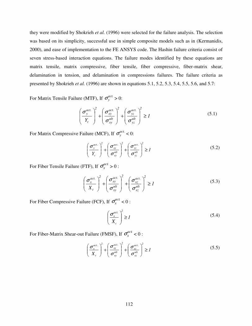
112
they were modified by Shokrieh et al. (1996) were selected for the failure analysis. The selection
was based on its simplicity, successful use in simple composite models such as in (Kermanidis,
2000), and ease of implementation to the FE ANSYS code. The Hashin failure criteria consist of
seven stress-based interaction equations. The failure modes identified by these equations are
matrix tensile, matrix compressive, fiber tensile, fiber compressive, fiber-matrix shear,
delamination in tension, and delamination in compressions failures. The failure criteria as
presented by Shokrieh et al. (1996) are shown in equations 5.1, 5.2, 5.3, 5.4, 5.5, 5.6, and 5.7:
For Matrix Tensile Failure (MTF), If .actyσ > 0:
1Y
2
ultyz
actyz
2
ultxy
actxy
2
t
acty
≥
+
+
σ
σ
σ
σσ ...
(5.1)
For Matrix Compressive Failure (MCF), If .actyσ < 0:
1Y
2
ult
yz
act
yz
2
ult
xy
act
xy
2
c
act
y≥
+
+
σ
σ
σ
σσ ...
(5.2)
For Fiber Tensile Failure (FTF), If .act
xσ > 0 :
1X
2
ultxz
actxz
2
ultxy
actxy
2
t
actx ≥
+
+
σ
σ
σ
σσ ...
(5.3)
For Fiber Compressive Failure (FCF), If .act
xσ < 0 :
1X
2
c
act
x ≥
.σ
(5.4)
For Fiber-Matrix Shear-out Failure (FMSF), If .act
xσ < 0 :
1X
2
ult
xz
act
xz
2
ult
xy
act
xy
2
t
act
x ≥
+
+
σ
σ
σ
σσ ...
(5.5)
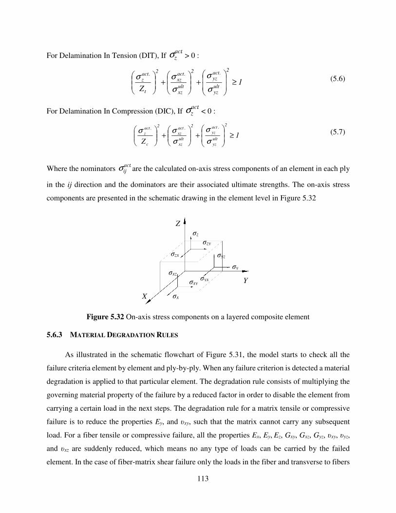
113
For Delamination In Tension (DIT), If .act
zσ > 0 :
1Z
2
ultyz
actyz
2
ultxz
actxz
2
t
actz ≥
+
+
σ
σ
σ
σσ...
(5.6)
For Delamination In Compression (DIC), If .act
zσ < 0 :
1Z
2
ult
yz
act
yz
2
ult
xz
act
xz
2
c
act
z ≥
+
+
σ
σ
σ
σσ...
(5.7)
Where the nominators .actijσ are the calculated on-axis stress components of an element in each ply
in the ij direction and the dominators are their associated ultimate strengths. The on-axis stress
components are presented in the schematic drawing in the element level in Figure 5.32
Figure 5.32 On-axis stress components on a layered composite element
5.6.3 MATERIAL DEGRADATION RULES
As illustrated in the schematic flowchart of Figure 5.31, the model starts to check all the
failure criteria element by element and ply-by-ply. When any failure criterion is detected a material
degradation is applied to that particular element. The degradation rule consists of multiplying the
governing material property of the failure by a reduced factor in order to disable the element from
carrying a certain load in the next steps. The degradation rule for a matrix tensile or compressive
failure is to reduce the properties Ey, and υxy, such that the matrix cannot carry any subsequent
load. For a fiber tensile or compressive failure, all the properties Ex, Ey, Ez, Gxy, Gxz, Gyz, υxy, υyz,
and υxz are suddenly reduced, which means no any type of loads can be carried by the failed
element. In the case of fiber-matrix shear failure only the loads in the fiber and transverse to fibers
X
Y
Z
σzx
σzy
σz
σyx
σy
σyz
σx
σxy
σxz

114
direction can be carried, this is achieved by reducing the values of Gxy, and υxy. The delamination
failure in tension or compression has two modes, the first mode affects the carrying capacity of
the laminate in the z direction, and the second mode affects the interlaminar shear carrying capacity
between the layers. Therefore, the properties Ez, Gyz, Gxz, υyz, and υxz must be reduced.
5.6.4 SHEAR TEST SIMULATION
A finite element simulation of the three points loading test was performed for the cores A1-
CH-W and A2-CH-CP. The boundary conditions applied to the core structure were hinged and
roller supports spaced 610 mm (24 in), and similar to that conducted in the experimental testing.
A linearly increasing load protocol was applied in the center of the top skin to an area equals to
the rectangular steel loading plate contact with the specimen. An incremental value of 5 kN up to
a total load of 350 kN is applied on the beam. Only quarter of the beam geometry was created and
two planes of symmetry are assumed in order to reduce the computational time.
The progressive failure modeling of both cores A1-HC-W and A2-HC-CP showed an
agreement with the delamination failure mode due interlaminar shear detected in the experimental
work, such that the stress-component σyz has the highest value and the major contribution in the
delamination failure. Figures 5.33.a, b, and c show the damage propagation predicted by the core
A1-HC-W model before failure during a three points loading application at the load steps 90 kN,
95 kN, and 100 kN, respectively. The pictures show a quarter section of the core where a
delimitation failure is propagating between the core and the skin surfaces. In addition, a
comparison between the numbers of the accumulated failed elements by each failure criterion per
load step is presented in the charts for the three different load steps. Figure 5.34.a, and 5.34.b
present the failed elements under delamination in tension and compression of both cores A1-HC-
W and A2-HC-CP, respectively. It can be noticed that the progressive model was able to depict
the observed mode of failure in the experimental test. In addition, Figure 5.35 shows the degraded
elements between the core structure and the upper skin, which resulted in a partial separation just
near the machine loading foot print.
In the finite element validation, the total core failure is recorded at 10 percent change in the
slope of the load-deflection curve. A summary of the validation results of the FE element
progressive model degradation with experimental work is presented in Table 5.9.
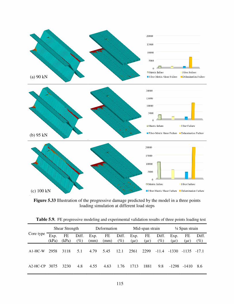
115
Figure 5.33 Illustration of the progressive damage predicted by the model in a three points loading simulation at different load steps
Table 5.9. FE progressive modeling and experimental validation results of three points loading test
Core type Shear Strength Deformation Mid-span strain ¼ Span strain
Exp. (kPa)
FE (kPa)
Diff. (%)
Exp. (mm)
FE (mm)
Diff. (%)
Exp. (µɛ)
FE (µɛ)
Diff. (%)
Exp. (µɛ)
FE (µɛ)
Diff. (%)
A1-HC-W 2958 3118 5.1 4.79 5.45 12.1 2561 2299 -11.4 -1330 -1135 -17.1
A2-HC-CP 3075 3230 4.8 4.55 4.63 1.76 1713 1881 9.8 -1298 -1410 8.6
(b) 95 kN
(c) 100 kN
(a) 90 kN
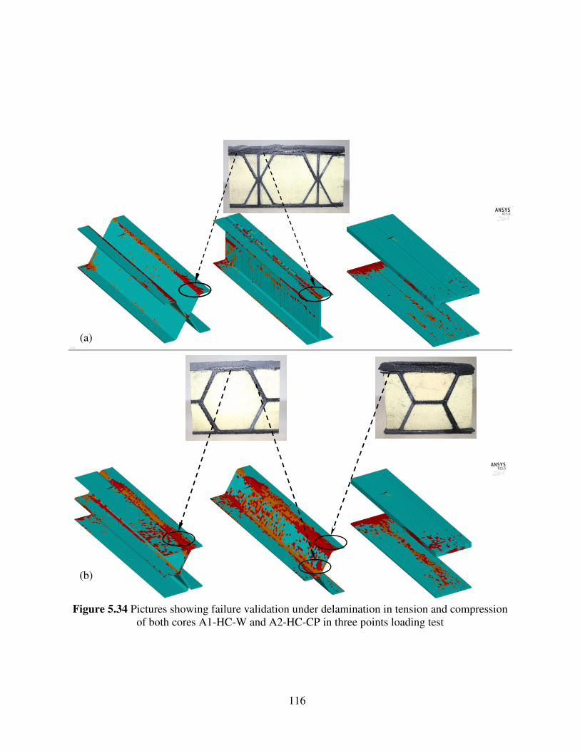
116
Figure 5.34 Pictures showing failure validation under delamination in tension and compression
of both cores A1-HC-W and A2-HC-CP in three points loading test
(a)
(b)
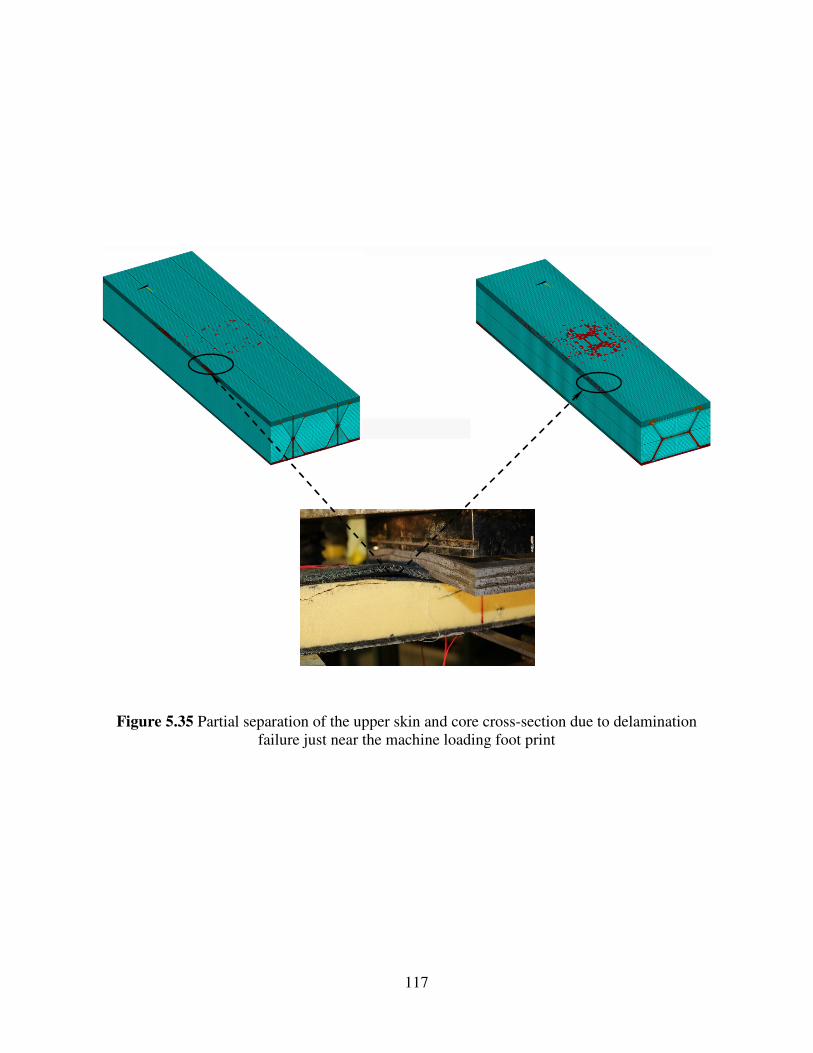
117
Figure 5.35 Partial separation of the upper skin and core cross-section due to delamination failure just near the machine loading foot print
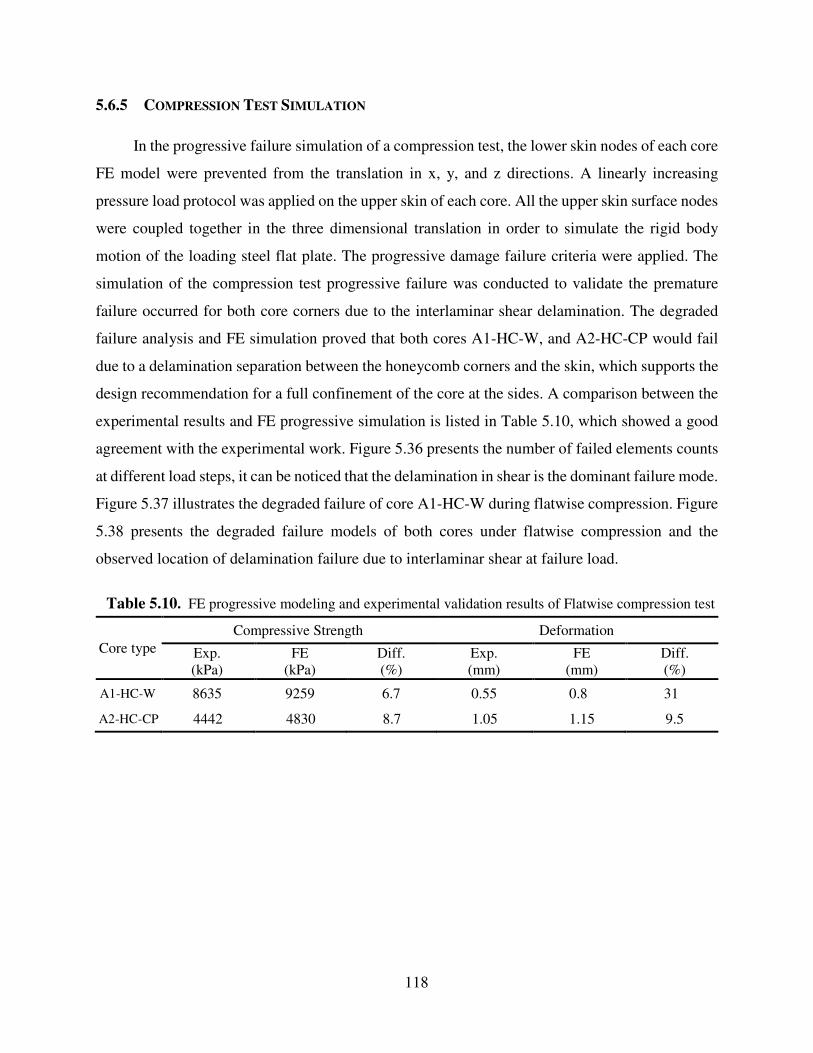
118
5.6.5 COMPRESSION TEST SIMULATION
In the progressive failure simulation of a compression test, the lower skin nodes of each core
FE model were prevented from the translation in x, y, and z directions. A linearly increasing
pressure load protocol was applied on the upper skin of each core. All the upper skin surface nodes
were coupled together in the three dimensional translation in order to simulate the rigid body
motion of the loading steel flat plate. The progressive damage failure criteria were applied. The
simulation of the compression test progressive failure was conducted to validate the premature
failure occurred for both core corners due to the interlaminar shear delamination. The degraded
failure analysis and FE simulation proved that both cores A1-HC-W, and A2-HC-CP would fail
due to a delamination separation between the honeycomb corners and the skin, which supports the
design recommendation for a full confinement of the core at the sides. A comparison between the
experimental results and FE progressive simulation is listed in Table 5.10, which showed a good
agreement with the experimental work. Figure 5.36 presents the number of failed elements counts
at different load steps, it can be noticed that the delamination in shear is the dominant failure mode.
Figure 5.37 illustrates the degraded failure of core A1-HC-W during flatwise compression. Figure
5.38 presents the degraded failure models of both cores under flatwise compression and the
observed location of delamination failure due to interlaminar shear at failure load.
Table 5.10. FE progressive modeling and experimental validation results of Flatwise compression test
Core type Compressive Strength Deformation
Exp. (kPa)
FE (kPa)
Diff. (%)
Exp. (mm)
FE (mm)
Diff. (%)
A1-HC-W 8635 9259 6.7 0.55 0.8 31
A2-HC-CP 4442 4830 8.7 1.05 1.15 9.5
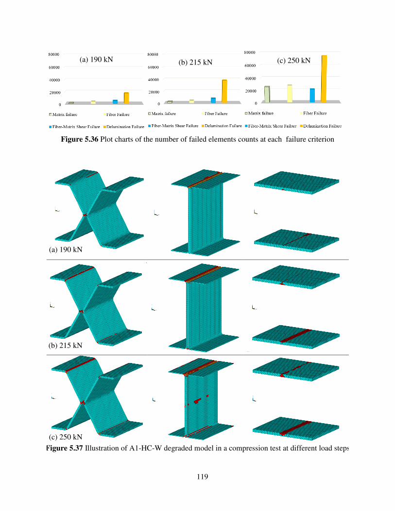
119
Figure 5.36 Plot charts of the number of failed elements counts at each failure criterion
Figure 5.37 Illustration of A1-HC-W degraded model in a compression test at different load steps
(b) 215 kN
(c) 250 kN
(a) 190 kN
(b) 215 kN (c) 250 kN (a) 190 kN
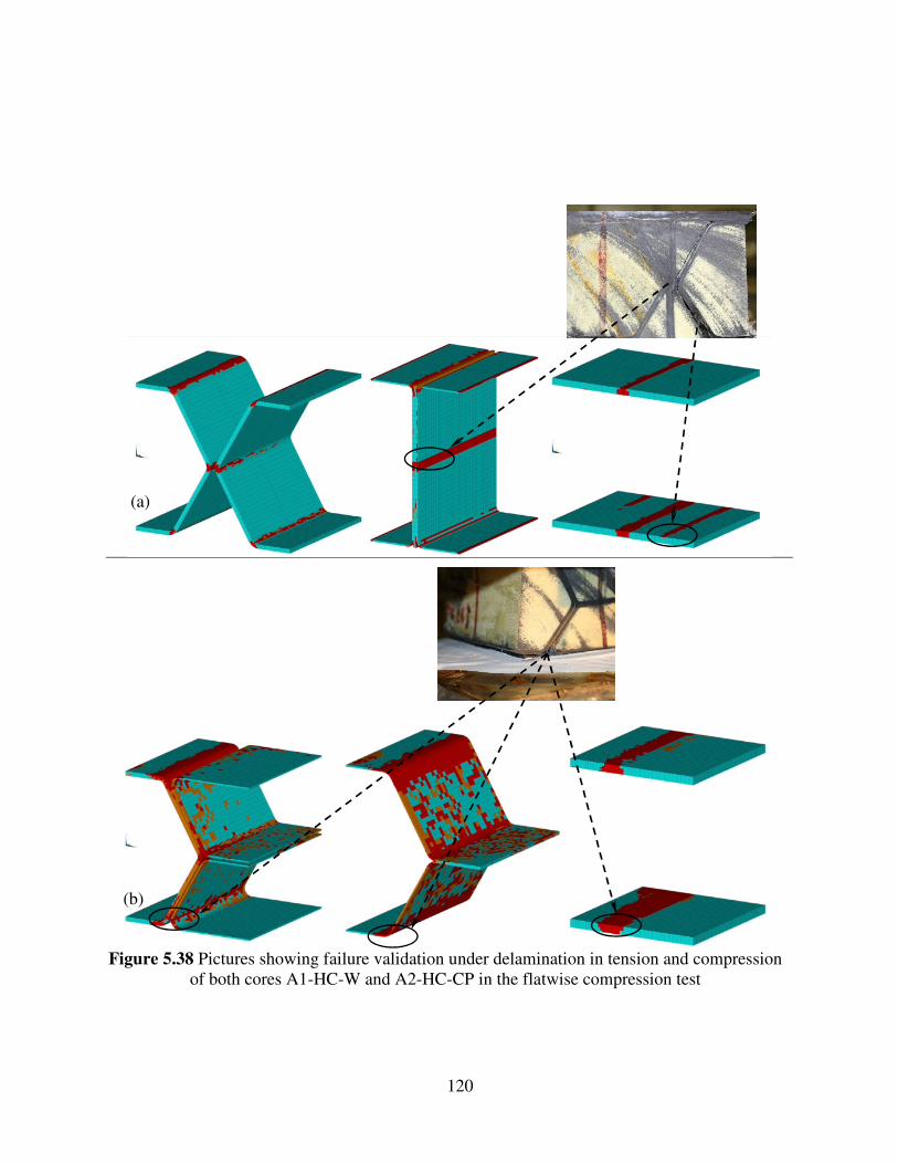
120
Figure 5.38 Pictures showing failure validation under delamination in tension and compression
of both cores A1-HC-W and A2-HC-CP in the flatwise compression test
(a)
(b)
121
5.7 SUMMARY AND DESIGN RECOMMENDATIONS
Based on the experimental testing results and the degraded numerical validation, guidelines are
presented for the design of light weight composite cores with honeycomb beams that are
configured in different structural geometries. In addition, performance charts and presented for the
designer in order to select the appropriate honeycomb bas ed sandwich core out of a variety of core
selections in the literature.
For the shear strength, it is worth noting that the similar shear performance achieved by cores
A1-HC-W and A2-HC-CP with the balsa system was based on a carbon/epoxy laminate that is
nearly of 35 MPa shear strength capacity, see Figure 5.36. On the other hand, the carbon fibers
and resin formulation used to fabricate the webbed cores developed by Robinson and Kosmatka
(2008) provided a 386 MPa shear strength. Core A1-HC-W failed due to delamination of
interlaminar shear between the core and the skin surfaces. This mode of failure represents the
maximum shear strength that can be carried by this core structural configuration. Another epoxy
formulation that could provide only an average value of shear strength between the two previously
mentioned values would expect to highly increase the shear strength of the fabricated core. In
addition, the material cost and consequently fabrication cost would not be highly increased when
compared to the webbed cores that were fabricated using a special epoxy formulation.
The fabrication of core A1-HC-W experienced three different trials using the SCRIMP
technique with different infusion strategies until a succesful infusion was achevied, this resulted
in a consumption of large amounts of resin and reinforcing fiber materials. The difficulty of having
a successful infusion of core A1-HC-W using the SCRIMP technique can be attributed to the
existence of several non straight and vertical flow baths, i.e. core webs, within the core cross-
section. Moreover, the successful trial achieved a non uniform distribution of the resin all over the
core cross-section width, which resulted in a variable fiber volume fraction, hence a relative
difference in webs stiffnesses. The torsional moment detected at the end of the core shear test can
be attributed to the existence of variation of webs stiffness. Therefore, it is recommended to
fabricate the sandwich composite cores that have a similar construction of flow paths using the
FRIM, or OOA processing methods. For the FRIM processing method, no special tools is used
other than that used for the SCRIMP technique. Using the resin films to infuse the core webs will

122
ensure a highly uniform resin distribution and full wetting of the inside core fibers, and at the same
time, the capability of manufacturing large-scale structures will be maintained. The OOA would
provide the highest quality of fiber/epoxy laminates within the core cross-section, and its
applicable for manufacturing these type of cores as the service temperature of the used foam is
higher than 150 Cº. This would make it possible to use the prepregs. The only concern for the
FRIM and OOA application is the relative cost of material, which can be minimized through an
optimized laminate thickness.
Both the honeycomb and the trapezoidal shaped beams of core A2-HC-CP were wrapped with
different number of carbon layers in order to construct the web laminate thickness and to distibute
the shear forces into the skin in both sides of the web. Despite doing this, the core failed in
delamination due to interlaminar shear for both core cuts; and it was found that the distibuted
number of continuous layers from the webs into the skin has a high contribution in the equal
distribution of shear forces. Therefore, for core webs spaced 80 mm as in core A2-HC-CP, it is
recommended to equally interleave the continous fibers from the webs into the skin, such that a
concentration of shear forces over a single side of the skin can be avoided.
From the flatwise compression test, it was found that both cores A1-HC-W and A2-HC-CP
would experience a premature failure due to delamination of interlaminar shear at the core sides.
In addition, the core laminate webs will not function to its ultimate compressive capacity. Finding
this, a full confinement of the core sides is recommended by overlapping the upper and lower skins
at the core sides as well as the full wrapping of the side foam beams. This will ensure higher
compressive stresses of the core webs. By satisfying this recommendation and the consideration
of full web compressive capacity, core A1-HC-W and core A2-HC-CP would achieve 2.04 and
1.3 times increase in compressive capacity than the balsa core, and lighter by nearly 36% and 49%,
respectively. In addition, core A1-HC-W would have 1.17 times increase in the compressive
capacity than core C4-TC, which is considered the highest compressive strength achieved for a
deployable bridge deck core in the literature.
In order to aid for the core selection from a strength prespective, a plot of the shear strength,
compressive strength of the cores A1-HC-W and A2-HC-CP as well as the predicted compressive
strength after satisfying the recommendation of wrapping the core sides is presented in Figure
5.39, the values are compared to the balsa-baseline performance and all webbed cores presented
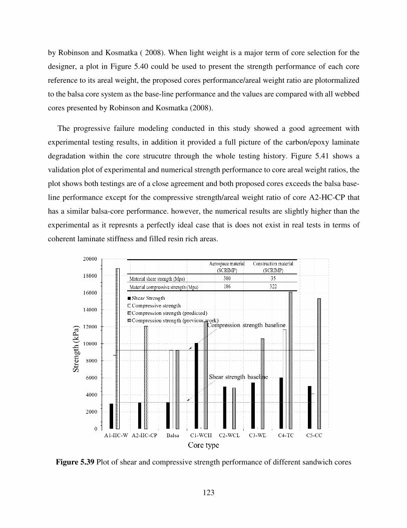
123
by Robinson and Kosmatka ( 2008). When light weight is a major term of core selection for the
designer, a plot in Figure 5.40 could be used to present the strength performance of each core
reference to its areal weight, the proposed cores performance/areal weight ratio are plotormalized
to the balsa core system as the base-line performance and the values are compared with all webbed
cores presented by Robinson and Kosmatka (2008).
The progressive failure modeling conducted in this study showed a good agreement with
experimental testing results, in addition it provided a full picture of the carbon/epoxy laminate
degradation within the core strucutre through the whole testing history. Figure 5.41 shows a
validation plot of experimental and numerical strength performance to core areal weight ratios, the
plot shows both testings are of a close agreement and both proposed cores exceeds the balsa base-
line performance except for the compressive strength/areal weight ratio of core A2-HC-CP that
has a similar balsa-core performance. however, the numerical results are slightly higher than the
experimental as it represnts a perfectly ideal case that is does not exist in real tests in terms of
coherent laminate stiffness and filled resin rich areas.
Figure 5.39 Plot of shear and compressive strength performance of different sandwich cores
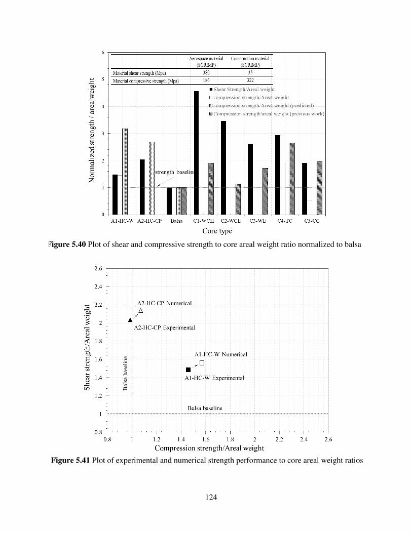
124
Figure 5.40 Plot of shear and compressive strength to core areal weight ratio normalized to balsa
Figure 5.41 Plot of experimental and numerical strength performance to core areal weight ratios
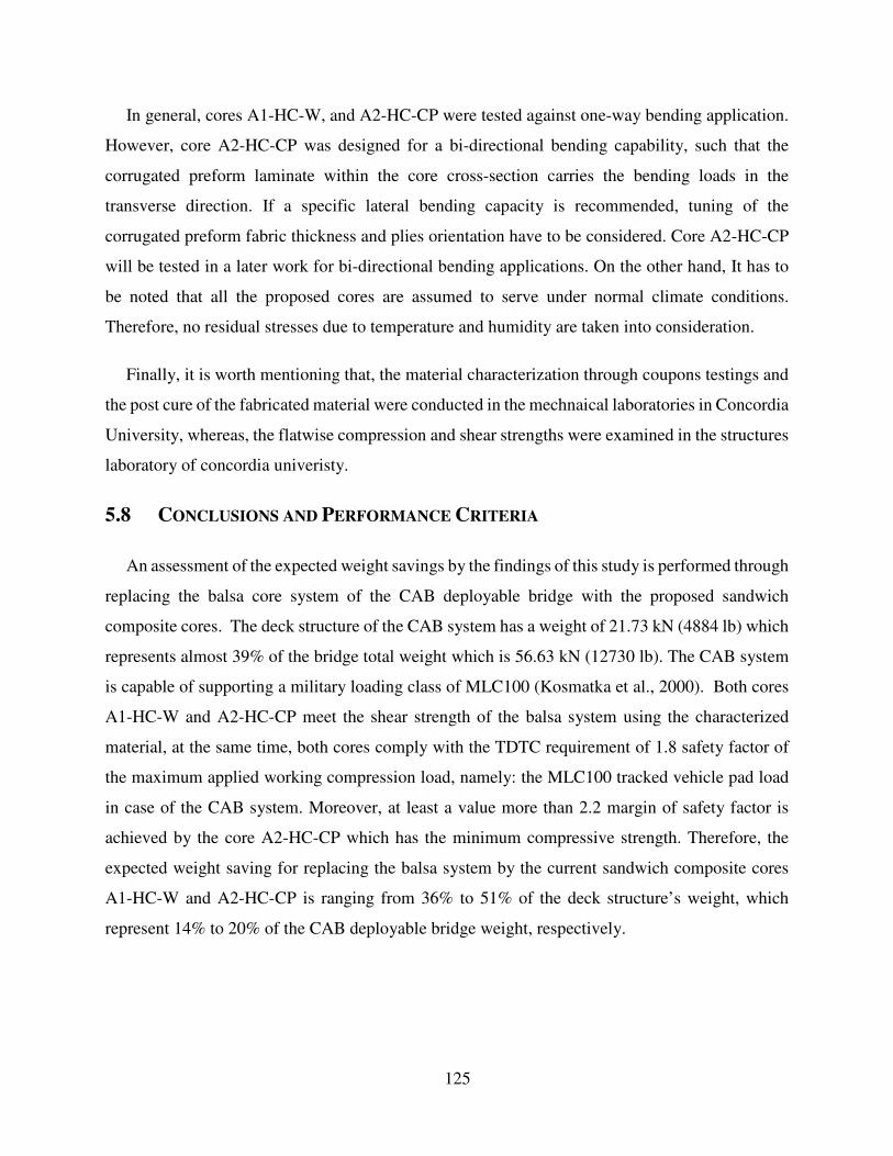
125
In general, cores A1-HC-W, and A2-HC-CP were tested against one-way bending application.
However, core A2-HC-CP was designed for a bi-directional bending capability, such that the
corrugated preform laminate within the core cross-section carries the bending loads in the
transverse direction. If a specific lateral bending capacity is recommended, tuning of the
corrugated preform fabric thickness and plies orientation have to be considered. Core A2-HC-CP
will be tested in a later work for bi-directional bending applications. On the other hand, It has to
be noted that all the proposed cores are assumed to serve under normal climate conditions.
Therefore, no residual stresses due to temperature and humidity are taken into consideration.
Finally, it is worth mentioning that, the material characterization through coupons testings and
the post cure of the fabricated material were conducted in the mechnaical laboratories in Concordia
University, whereas, the flatwise compression and shear strengths were examined in the structures
laboratory of concordia univeristy.
5.8 CONCLUSIONS AND PERFORMANCE CRITERIA
An assessment of the expected weight savings by the findings of this study is performed through
replacing the balsa core system of the CAB deployable bridge with the proposed sandwich
composite cores. The deck structure of the CAB system has a weight of 21.73 kN (4884 lb) which
represents almost 39% of the bridge total weight which is 56.63 kN (12730 lb). The CAB system
is capable of supporting a military loading class of MLC100 (Kosmatka et al., 2000). Both cores
A1-HC-W and A2-HC-CP meet the shear strength of the balsa system using the characterized
material, at the same time, both cores comply with the TDTC requirement of 1.8 safety factor of
the maximum applied working compression load, namely: the MLC100 tracked vehicle pad load
in case of the CAB system. Moreover, at least a value more than 2.2 margin of safety factor is
achieved by the core A2-HC-CP which has the minimum compressive strength. Therefore, the
expected weight saving for replacing the balsa system by the current sandwich composite cores
A1-HC-W and A2-HC-CP is ranging from 36% to 51% of the deck structure’s weight, which
represent 14% to 20% of the CAB deployable bridge weight, respectively.
126
CHAPTER 6
Strength Optimization of Composite
Deployable Bridge Decks
6.1 INTRODUCTION
The use of composite materials in many structural applications is found to be very advantageous
as they provided high strength to weight ratio. Although composites are excellent replacement of
metallic materials in the application of deployable bridges, as proved in Chapter 5, the analysis
and design of composite structures is very complex compared with the metallic structures. A
remarkable benefit of using composites is the capability of varying the material orthotropic
properties to meet a specific structural need. In addition, minimizing weight and cost are other
factors that can be taken into consideration, laminate stacking sequence (ply orientation) is the
main design variable to control and achieve these designs objectives. The possibility of reaching
an effective design while satisfying multiple failure criteria and the difficulty of obtaining the best
design values out of a large set of design variables make design optimization the efficient tool for
satisfying the design requirement. For a deployable bridge application, structural laminates in the
composite decks are subjected to multiple loading conditions that cannot be represented in a
laboratory test except in the scaled structure prototypes. For instance, a biaxial load in tension and
compression can significantly decrease the compressive strength of a unidirectional composite
laminate. Therefore, the maximum strength design optimization of sandwich composite decks
while considering different types of loading conditions is investigated in this Chapter. Standard
PSO and the proposed algorithm CD-PSO are modified to meet the discrete nature of composites
design. Moreover, the CD-PSO is integrated with the Harmony search technique and a fly-back
mechanism to handle the constraints violation and redirect the swarm search into feasible regions.
The developed algorithm is named HCD-PSO. A computationally efficient analytical model
implementing the Classical Lamination Theory (CLT) is developed. The stacking sequence of the
6
127
laminate fibers is considered as the design variable to maximize the margin of failure with respect
to the applied loadings. The failure analysis is conducted using the Tsai-Wu failure criterion.
In this chapter, the design approach of composite laminates and the design safety factors
recommended by the Trilateral Design and Testing Code (TDTC, 2005) for deployable bridges are
clarified. Analysis of the maximum applied loads of different MLC vehicle classes on a deployable
bridge structure of 12 m is presented and the corresponding applied loads on the sandwich core
are demonstrated. Following, the stress and strain laminate analysis using the Classical
Lamination Theory (CLT) in composite plates is briefly described. The optimization problem
formulation for the maximum strength design of composites using the HCD-PSO algorithm is
represented. Finally, the standard PSO and CD-PSO are applied and a comparison of the results is
summarized.
6.2 DESIGN APPROACH
The design approach of the composite deployable bridges follows a Limit State Design
provisions (LSD), the design criteria deals with the relationship of:
(a) Stresses and strains occurring in a structural material under an external applied loads,
(b) Stresses and strain capacities of the structural material element,
(c) Separation between the actual stresses and strains values and the structural material
capacity by an acceptable factor of safety.
The relationship concept for the imposed load and the material resistance can be clarified as in
Figure 6.1 in the shape of bell curves distribution along with the design limits, in which, the design
loads (working loads) are taken as the maximum expected static loads of the hypothetical vehicles
based on TDTC requirements or real vehicle loads of the same loading class, these working loads
take into account the impact, side-slope and eccentricity factors. The design properties of the
composite materials are determined from coupon tests and derived using a standard statistical tests
of the test data values. The B-basis allowable property is the statistical test that is used to derive
the material design property of sandwich composite cores, in which 90% reliability of the
fabricated material will not fail at the allowable strength value. This is represented as follows
( )dvavbasisB SN ⋅−=− .σσ (6.1)
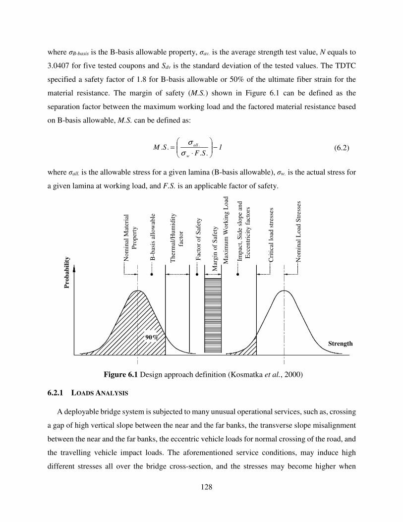
128
where σB-basis is the B-basis allowable property, σav. is the average strength test value, N equals to
3.0407 for five tested coupons and Sdv is the standard deviation of the tested values. The TDTC
specified a safety factor of 1.8 for B-basis allowable or 50% of the ultimate fiber strain for the
material resistance. The margin of safety (M.S.) shown in Figure 6.1 can be defined as the
separation factor between the maximum working load and the factored material resistance based
on B-basis allowable, M.S. can be defined as:
1SF
SMw
all −
⋅=
.... .
σ
σ (6.2)
where σall. is the allowable stress for a given lamina (B-basis allowable), σw. is the actual stress for
a given lamina at working load, and F.S. is an applicable factor of safety.
Figure 6.1 Design approach definition (Kosmatka et al., 2000)
6.2.1 LOADS ANALYSIS
A deployable bridge system is subjected to many unusual operational services, such as, crossing
a gap of high vertical slope between the near and the far banks, the transverse slope misalignment
between the near and the far banks, the eccentric vehicle loads for normal crossing of the road, and
the travelling vehicle impact loads. The aforementioned service conditions, may induce high
different stresses all over the bridge cross-section, and the stresses may become higher when
Nom
inal
Loa
d St
ress
es
Cri
tical
load
str
esse
s
Im
pact
, Sid
e sl
ope
and
Ecc
entr
icity
fac
tors
Mar
gin
of S
afet
y
Fac
tor
of S
afet
y
B-b
asis
allo
wab
le
Nom
inal
Mat
eria
l Pr
oper
ty
The
rmal
/Hum
idity
fa
ctor
Pro
ba
bil
ity
Strength 90%
Max
imum
Wor
king
Loa
d
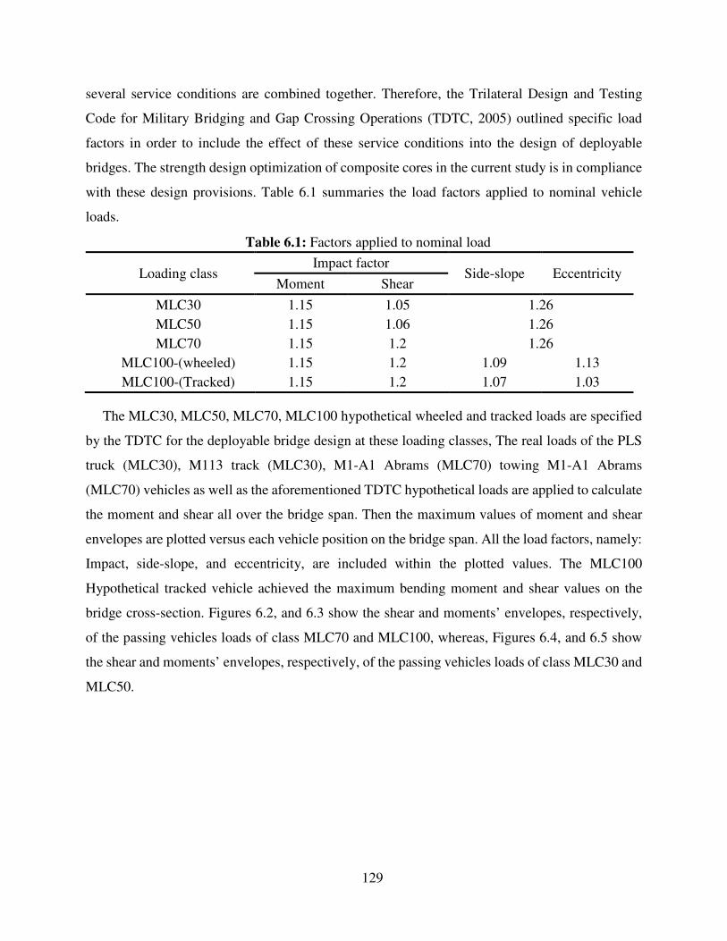
129
several service conditions are combined together. Therefore, the Trilateral Design and Testing
Code for Military Bridging and Gap Crossing Operations (TDTC, 2005) outlined specific load
factors in order to include the effect of these service conditions into the design of deployable
bridges. The strength design optimization of composite cores in the current study is in compliance
with these design provisions. Table 6.1 summaries the load factors applied to nominal vehicle
loads.
Table 6.1: Factors applied to nominal load
Loading class Impact factor
Side-slope Eccentricity Moment Shear
MLC30 1.15 1.05 1.26 MLC50 1.15 1.06 1.26 MLC70 1.15 1.2 1.26
MLC100-(wheeled) 1.15 1.2 1.09 1.13 MLC100-(Tracked) 1.15 1.2 1.07 1.03
The MLC30, MLC50, MLC70, MLC100 hypothetical wheeled and tracked loads are specified
by the TDTC for the deployable bridge design at these loading classes, The real loads of the PLS
truck (MLC30), M113 track (MLC30), M1-A1 Abrams (MLC70) towing M1-A1 Abrams
(MLC70) vehicles as well as the aforementioned TDTC hypothetical loads are applied to calculate
the moment and shear all over the bridge span. Then the maximum values of moment and shear
envelopes are plotted versus each vehicle position on the bridge span. All the load factors, namely:
Impact, side-slope, and eccentricity, are included within the plotted values. The MLC100
Hypothetical tracked vehicle achieved the maximum bending moment and shear values on the
bridge cross-section. Figures 6.2, and 6.3 show the shear and moments’ envelopes, respectively,
of the passing vehicles loads of class MLC70 and MLC100, whereas, Figures 6.4, and 6.5 show
the shear and moments’ envelopes, respectively, of the passing vehicles loads of class MLC30 and
MLC50.
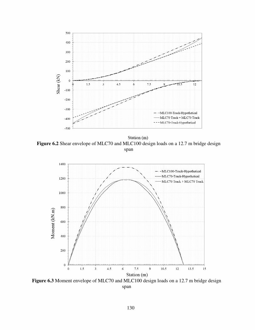
130
Figure 6.2 Shear envelope of MLC70 and MLC100 design loads on a 12.7 m bridge design
span
Figure 6.3 Moment envelope of MLC70 and MLC100 design loads on a 12.7 m bridge design
span
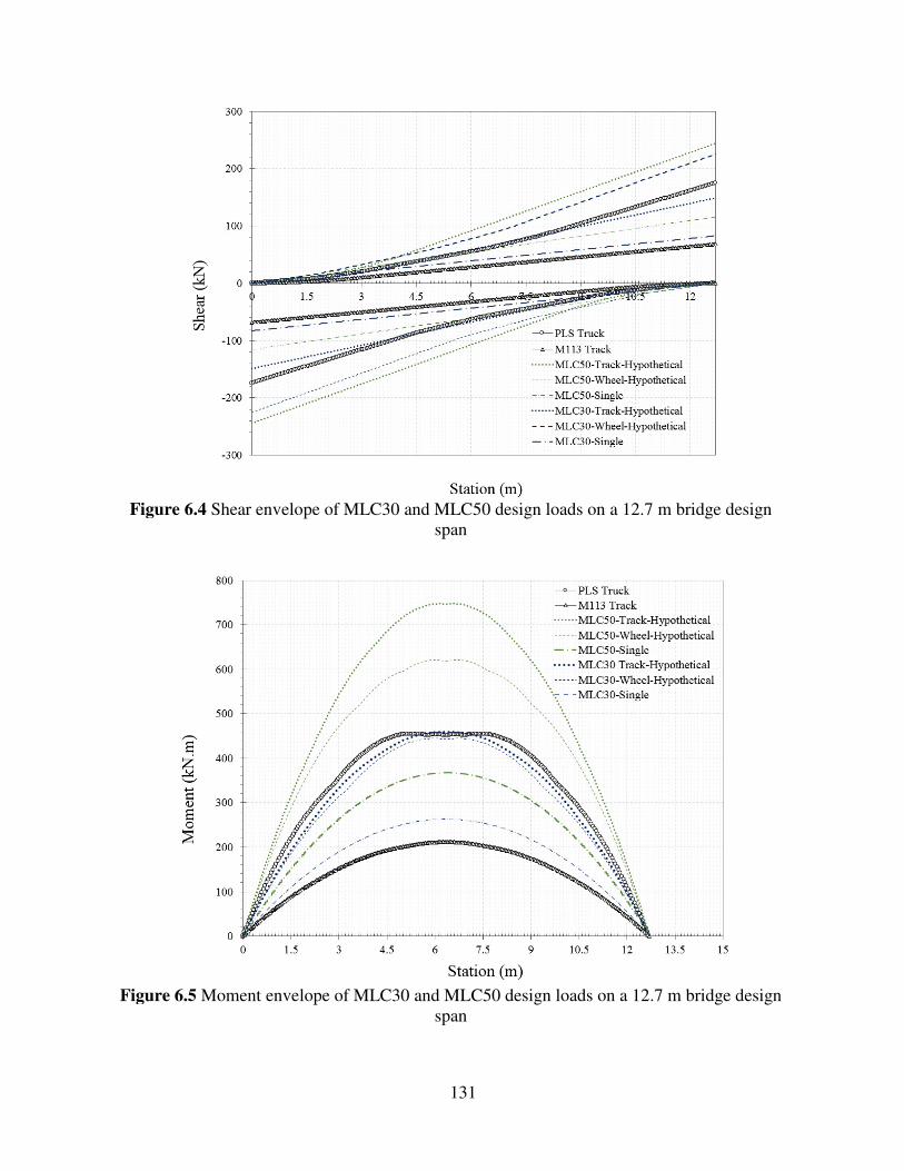
131
Figure 6.4 Shear envelope of MLC30 and MLC50 design loads on a 12.7 m bridge design
span
Figure 6.5 Moment envelope of MLC30 and MLC50 design loads on a 12.7 m bridge design
span
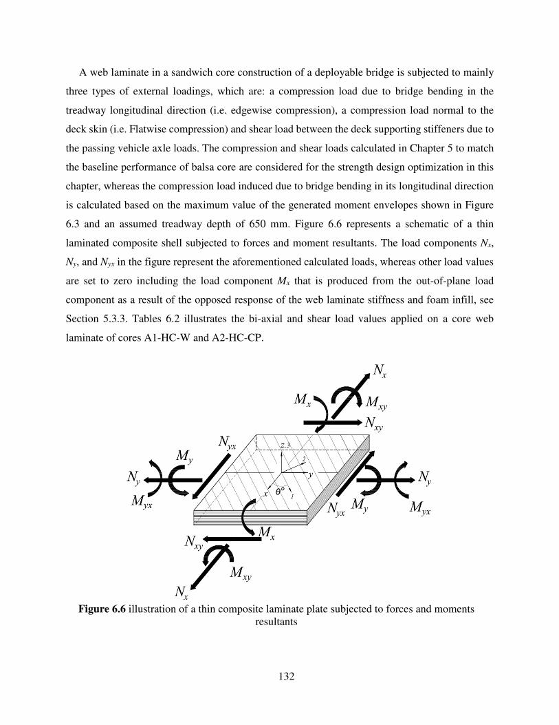
132
A web laminate in a sandwich core construction of a deployable bridge is subjected to mainly
three types of external loadings, which are: a compression load due to bridge bending in the
treadway longitudinal direction (i.e. edgewise compression), a compression load normal to the
deck skin (i.e. Flatwise compression) and shear load between the deck supporting stiffeners due to
the passing vehicle axle loads. The compression and shear loads calculated in Chapter 5 to match
the baseline performance of balsa core are considered for the strength design optimization in this
chapter, whereas the compression load induced due to bridge bending in its longitudinal direction
is calculated based on the maximum value of the generated moment envelopes shown in Figure
6.3 and an assumed treadway depth of 650 mm. Figure 6.6 represents a schematic of a thin
laminated composite shell subjected to forces and moment resultants. The load components Nx,
Ny, and Nyx in the figure represent the aforementioned calculated loads, whereas other load values
are set to zero including the load component Mx that is produced from the out-of-plane load
component as a result of the opposed response of the web laminate stiffness and foam infill, see
Section 5.3.3. Tables 6.2 illustrates the bi-axial and shear load values applied on a core web
laminate of cores A1-HC-W and A2-HC-CP.
Figure 6.6 illustration of a thin composite laminate plate subjected to forces and moments
resultants
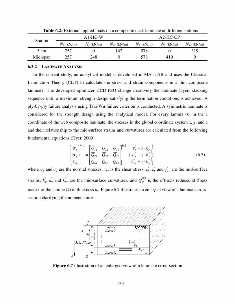
133
Table 6.2: External applied loads on a composite deck laminate at different stations
Station A1-HC-W A2-HC-CP
Nx (kN/m) Ny (kN/m) Nyx (kN/m) Nx (kN/m) Ny (kN/m) Nyx (kN/m)
5 cm 257 0 142 578 0 319 Mid-span 257 248 0 578 419 0
6.2.2 LAMINATE ANALYSIS
In the current study, an analytical model is developed in MATLAB and uses the Classical
Lamination Theory (CLT) to calculate the stress and strain components in a thin composite
laminate. The developed optimizer HCD-PSO change iteratively the laminate layers stacking
sequence until a maximum strength design satisfying the termination conditions is achieved. A
ply-by-ply failure analysis using Tsai-Wu failure criterion is conducted. A symmetric laminate is
considered for the strength design using the analytical model. For every lamina (k) in the z
coordinate of the web composite laminate, the stresses in the global coordinate system x, y, and z
and their relationship to the mid-surface strains and curvatures are calculated from the following
fundamental equations (Hyer, 2009).
( ) ( )
⋅+
⋅+
⋅+
⋅
=
°°
°°
°°
xyxy
yy
xx
k
666261
262221
161211
k
xy
y
x
kz
kz
kz
QQQ
QQQ
QQQ
τ
ε
ε
τ
σ
σ
(6.3)
where σx andσy are the normal stresses, τxy is the shear stress, εx° , εy
° and γxy° are the mid-surface
strains, kx° , ky
° and kxy° are the mid-surface curvatures, and Qd
ij
(k) is the off-axis reduced stiffness
matrix of the lamina (k) of thickness hk. Figure 6.7 illustrates an enlarged view of a laminate cross-
section clarifying the nomenclature.
Figure 6.7 illustration of an enlarged view of a laminate cross-section
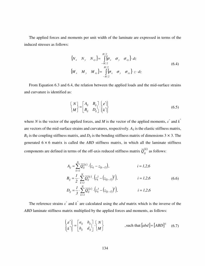
134
The applied forces and moments per unit width of the laminate are expressed in terms of the
induced stresses as follows:
{ } { } dzNNN
2H
2H
xyyxxyyx ⋅= ∫−
σσσ
{ } { } dzzMMM
2H
2H
xyyxxyyx ⋅⋅= ∫−
σσσ
(6.4)
From Equation 6.3 and 6.4, the relation between the applied loads and the mid-surface strains
and curvature is identified as:
⋅
=
°
°
kDB
BA
M
N
ijij
ijij ε (6.5)
where N is the vector of the applied forces, and M is the vector of the applied moments, ε° and k°
are vectors of the mid-surface strains and curvatures, respectively. Aij is the elastic stiffness matrix,
Bij is the coupling stiffness matrix, and Dij is the bending stiffness matrix of dimensions 3 × 3. The
generated 6 ×6 matrix is called the ABD stiffness matrix, in which all the laminate stiffness
components are defined in terms of the off-axis reduced stiffness matrix Qdij
(k) as follows:
( )( )( ) 621izzQA 1kk
N
1k
kijij ,, , =−⋅= −
=
∑
( )( )( )( ) 621izzQ
2
1B
2
1k2k
N
1k
kijij ,, , =−⋅⋅= −
=
∑
( )( )( )( ) 621izzQ
3
1D
3
1k3k
N
1k
kijij ,, , =−⋅⋅= −
=
∑
(6.6)
The reference strains ε° and k° are calculated using the abd matrix which is the inverse of the
ABD laminate stiffness matrix multiplied by the applied forces and moments, as follows:
[ ] [ ] 1- such that , ABDabdM
N
db
ba
k ijij
ijij=
⋅
=
°
°ε (6.7)
135
Hence the off-axis stresses σx,σy and τxy at each layer of the laminate are computed using
Equation 6.3. by performing a tonsorial transformation of trigonometric functions, the on-axis
stresses σ1,σ2 and τ12 at each layer (k) are calculated as follows:
( ) ( )k
xy
y
x
22
22
22k
12
2
1
nmmnmn
mn2mn
mn2nm
⋅
−−
−=
τ
σ
σ
τ
σ
σ
(6.8)
where m and n equal to cosϴ and sinϴ, respectively. By knowing the on-axis stresses, the Tsai-Wu
failure criterion is applied as described in the coming section.
6.2.3 FAILURE ANALYSIS
The Tsai-Wu failure criterion is chosen for the maximum strength design in the current study
due to its simplicity in this application, as well as its better ability of predicting the failure in a
multiple applied loading condition which is the case of the composite core web laminates. For the
state of plane stress analysis the failure occurs using Tsai-Wu criterion when the calculated stresses
reach the ultimate stresses g5:hi , such that the following equation is satisfied (Tsai and Wu,
1971):
( ) 1F2FFFFFF 211221266
2222
211122111221 =+++++= maxmaxmaxmaxmaxmaxmax , , σστσσσστσσ (6.9)
Therefore, the strength ratio to reach the ultimate stresses is identified as follows:
1SF2SFSFSFSFSF 212R12
212
2R66
22
2R22
21
2R112R21R1 =⋅⋅+⋅⋅+⋅⋅+⋅⋅+⋅⋅+⋅⋅ σστσσσσ (6.10)
Which can be shown in the form of a quadratic equation as:
01SBSA R2R =−⋅+⋅⋅ (6.11)
Where coefficients A, and B are equal to:
211221266
2222
2111 F2FFFA σστσσ ⋅⋅−⋅+⋅+⋅=
2211 FFB σσ ⋅+⋅=
136
The terms F1, F2, F11, F22, F66, and F12 are calculated as follows:
2211
2
66
ct
22
ct
2
ct
11
ct
1
FF2
1F
S
1F
YY
1F
Y
1
Y
1F
XX
1 F
X
1
X
1F
⋅−=
=
⋅−=
+=
⋅−=
+=
12
,
,
(6.12)
where Xt and Xc are the ultimate tensile and compressive strength in the fiber direction, Yt and Yc
are the ultimate tensile and compressive strength perpendicular to the fiber direction, and S is the
ultimate in-plane shear strength. Finally in order to achieve a feasible solution, the stress at every
point within the laminate thickness has to satisfy the following inequality constraint:
( ) 1F 1221 < , , τσσ (6.13)
Figure 6.8 shows the typical Tsai-Wu quadratic failure envelope with the condition of stress
state at different points on the failure envelope. It could be noticed that the initiation of the failure
mechanism is highly affected by an acting bi-axial loading, such that the cracks initiation could be
accelerated or slow based on the type of bi-axial loading compared to on-axis compressive or
tensile loading. In Figure 6.8.a and Figure 6.8.b, it can be noticed that a lamina subjected to on-
axis compressive load and lateral tensile load would fail due to initiated cracks faster than a lamina
subjected only to an axial compression load, respectively. Similarly, the crack is slowly initiated
in a lamina subjected to on-axis tensile loading and lateral compressive load than a lamina
subjected to only an off-axis tensile load, as shown in Figure 6.8.c, and Figure 6.8.d, respectively.
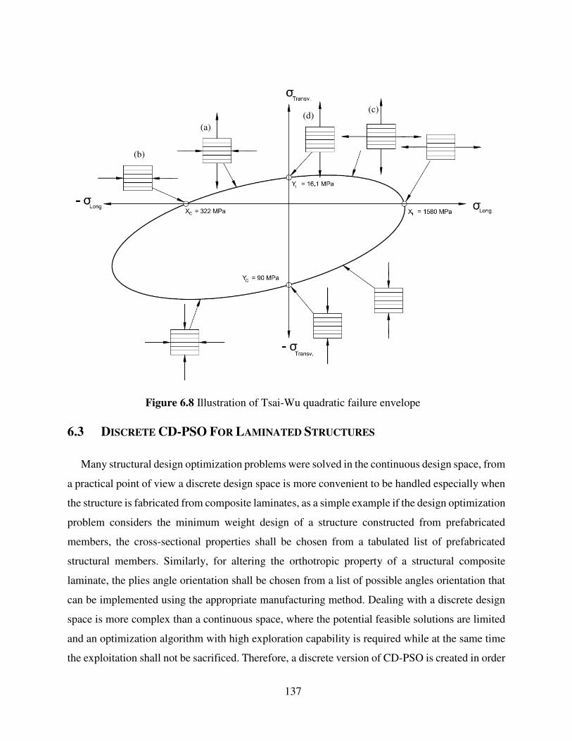
137
Figure 6.8 Illustration of Tsai-Wu quadratic failure envelope
6.3 DISCRETE CD-PSO FOR LAMINATED STRUCTURES
Many structural design optimization problems were solved in the continuous design space, from
a practical point of view a discrete design space is more convenient to be handled especially when
the structure is fabricated from composite laminates, as a simple example if the design optimization
problem considers the minimum weight design of a structure constructed from prefabricated
members, the cross-sectional properties shall be chosen from a tabulated list of prefabricated
structural members. Similarly, for altering the orthotropic property of a structural composite
laminate, the plies angle orientation shall be chosen from a list of possible angles orientation that
can be implemented using the appropriate manufacturing method. Dealing with a discrete design
space is more complex than a continuous space, where the potential feasible solutions are limited
and an optimization algorithm with high exploration capability is required while at the same time
the exploitation shall not be sacrificed. Therefore, a discrete version of CD-PSO is created in order
(b)
(a) (d) (c)
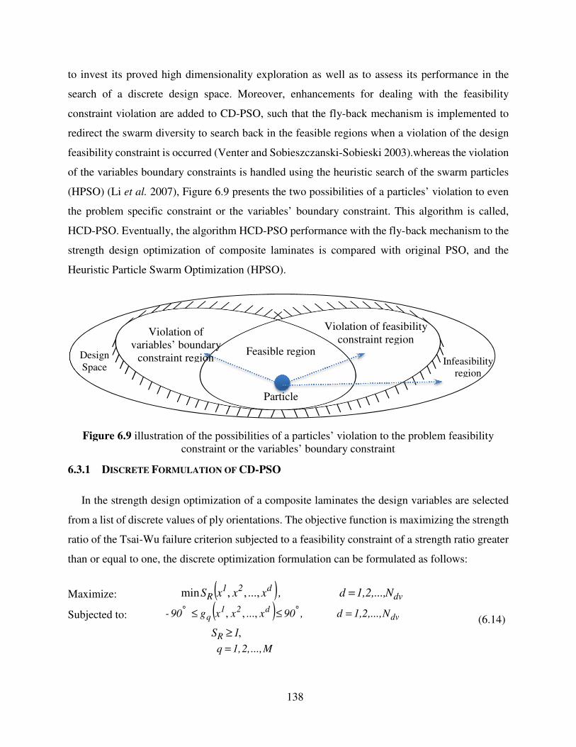
138
to invest its proved high dimensionality exploration as well as to assess its performance in the
search of a discrete design space. Moreover, enhancements for dealing with the feasibility
constraint violation are added to CD-PSO, such that the fly-back mechanism is implemented to
redirect the swarm diversity to search back in the feasible regions when a violation of the design
feasibility constraint is occurred (Venter and Sobieszczanski-Sobieski 2003).whereas the violation
of the variables boundary constraints is handled using the heuristic search of the swarm particles
(HPSO) (Li et al. 2007), Figure 6.9 presents the two possibilities of a particles’ violation to even
the problem specific constraint or the variables’ boundary constraint. This algorithm is called,
HCD-PSO. Eventually, the algorithm HCD-PSO performance with the fly-back mechanism to the
strength design optimization of composite laminates is compared with original PSO, and the
Heuristic Particle Swarm Optimization (HPSO).
Figure 6.9 illustration of the possibilities of a particles’ violation to the problem feasibility constraint or the variables’ boundary constraint
6.3.1 DISCRETE FORMULATION OF CD-PSO
In the strength design optimization of a composite laminates the design variables are selected
from a list of discrete values of ply orientations. The objective function is maximizing the strength
ratio of the Tsai-Wu failure criterion subjected to a feasibility constraint of a strength ratio greater
than or equal to one, the discrete optimization formulation can be formulated as follows:
Maximize: ( ) dvd21
R N 1,2,...,d ,x x xS =...,,,min
Subjected to: ( ) dvd21
q N 1,2,...,d ,90 x x xg 90- =≤≤ °° ...,,,
,1SR ≥ M..., 2, 1,q =
(6.14)
Violation of feasibility constraint region
Violation of variables’ boundary
constraint region Infeasibility region
Particle
Feasible region Design Space
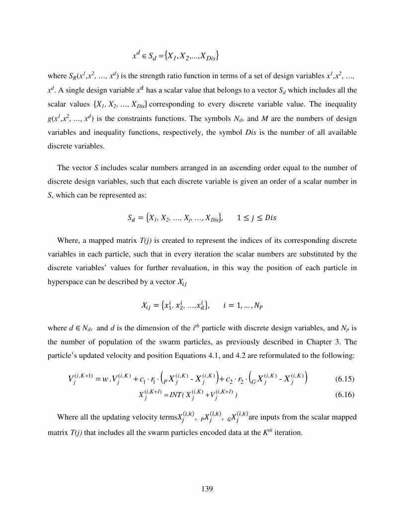
139
{ }Dis21dd
XXX Sx ,...,,=∈
where SR(x1,x2, …, xd) is the strength ratio function in terms of a set of design variables x1,x2, …,
xd. A single design variable xj has a scalar value that belongs to a vector Sd which includes all the
scalar values AX1, X2, …, XDisBcorresponding to every discrete variable value. The inequality
g(x1,x2, …, xd) is the constraints functions. The symbols Ndv and M are the numbers of design
variables and inequality functions, respectively, the symbol Dis is the number of all available
discrete variables.
The vector S includes scalar numbers arranged in an ascending order equal to the number of
discrete design variables, such that each discrete variable is given an order of a scalar number in
S, which can be represented as:
&j = nX1, X2, …, Xj, …, XDiso,1 ≤ q ≤ r�R Where, a mapped matrix T(j) is created to represent the indices of its corresponding discrete
variables in each particle, such that in every iteration the scalar numbers are substituted by the
discrete variables’ values for further revaluation, in this way the position of each particle in
hyperspace can be described by a vector X5� X5� = n��5 ,�G5 , …,�j5 o,� = 1,… ,sD
where d ∈Ndv and d is the dimension of the ith particle with discrete design variables, and Np is
the number of population of the swarm particles, as previously described in Chapter 3. The
particle’s updated velocity and position Equations 4.1, and 4.2 are reformulated to the following:
( ) ( ) - - . ),(),(22
),(),(11
),()1,( Kij
KijG
Kij
KijP
Kij
Kij XXrcXXrcVwV ⋅⋅+⋅⋅+=+
(6.15)
)V X( INT X1Ki
jKi
j1Ki
j),(),(),( ++
+= (6.16)
Where all the updating velocity terms��(5,u), �D �(5,u), �E �(5,u)are inputs from the scalar mapped
matrix T(j) that includes all the swarm particles encoded data at the Kth iteration.
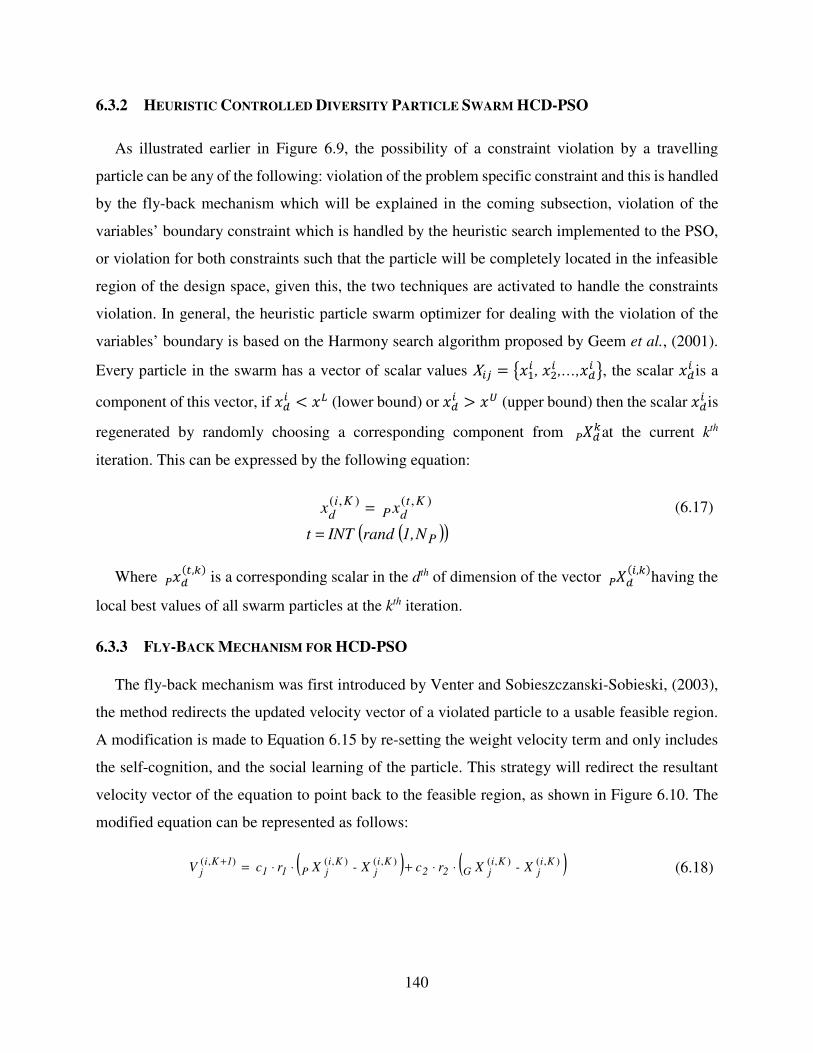
140
6.3.2 HEURISTIC CONTROLLED DIVERSITY PARTICLE SWARM HCD-PSO
As illustrated earlier in Figure 6.9, the possibility of a constraint violation by a travelling
particle can be any of the following: violation of the problem specific constraint and this is handled
by the fly-back mechanism which will be explained in the coming subsection, violation of the
variables’ boundary constraint which is handled by the heuristic search implemented to the PSO,
or violation for both constraints such that the particle will be completely located in the infeasible
region of the design space, given this, the two techniques are activated to handle the constraints
violation. In general, the heuristic particle swarm optimizer for dealing with the violation of the
variables’ boundary is based on the Harmony search algorithm proposed by Geem et al., (2001).
Every particle in the swarm has a vector of scalar values X5� = n��5 ,�G5 ,…,�j5 o, the scalar �j5 is a
component of this vector, if �j5 < �> (lower bound) or �j5 > �? (upper bound) then the scalar �j5 is
regenerated by randomly choosing a corresponding component from �D juat the current kth
iteration. This can be expressed by the following equation:
x xKt
dPKi
d),(),( = (6.17)
( )( ) N1, andr INT t P=
Where �D j(8,u) is a corresponding scalar in the dth of dimension of the vector �D j(5,u)having the
local best values of all swarm particles at the kth iteration.
6.3.3 FLY-BACK MECHANISM FOR HCD-PSO
The fly-back mechanism was first introduced by Venter and Sobieszczanski-Sobieski, (2003),
the method redirects the updated velocity vector of a violated particle to a usable feasible region.
A modification is made to Equation 6.15 by re-setting the weight velocity term and only includes
the self-cognition, and the social learning of the particle. This strategy will redirect the resultant
velocity vector of the equation to point back to the feasible region, as shown in Figure 6.10. The
modified equation can be represented as follows:
( ) ( ) X - X r c X - X r c VKi
jKi
jG22Ki
jKi
jP111Ki
j),(),(),(),(),( ⋅⋅+⋅⋅=+ (6.18)
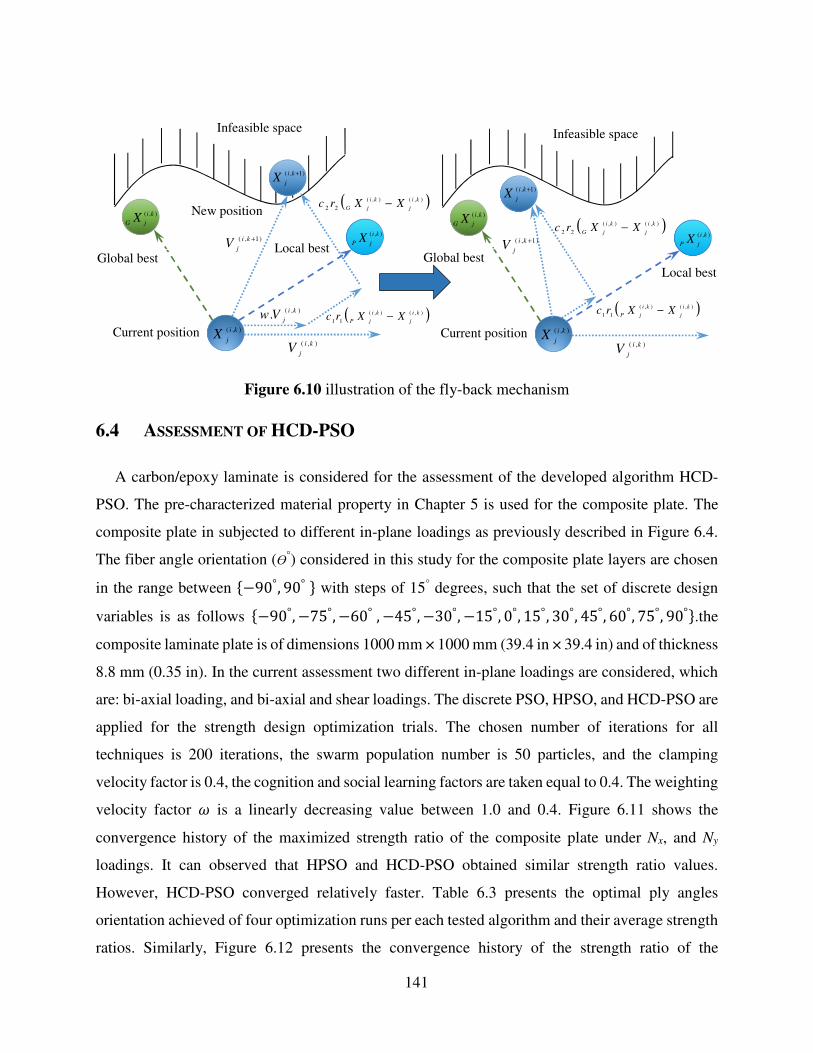
141
Figure 6.10 illustration of the fly-back mechanism
6.4 ASSESSMENT OF HCD-PSO
A carbon/epoxy laminate is considered for the assessment of the developed algorithm HCD-
PSO. The pre-characterized material property in Chapter 5 is used for the composite plate. The
composite plate in subjected to different in-plane loadings as previously described in Figure 6.4.
The fiber angle orientation (ϴ°) considered in this study for the composite plate layers are chosen
in the range between A−90°, 90°B with steps of 15° degrees, such that the set of discrete design
variables is as follows A−90°, −75°, −60°, −45°, −30°, −15°, 0°, 15°, 30°, 45°, 60°, 75°, 90°B.the
composite laminate plate is of dimensions 1000 mm × 1000 mm (39.4 in × 39.4 in) and of thickness
8.8 mm (0.35 in). In the current assessment two different in-plane loadings are considered, which
are: bi-axial loading, and bi-axial and shear loadings. The discrete PSO, HPSO, and HCD-PSO are
applied for the strength design optimization trials. The chosen number of iterations for all
techniques is 200 iterations, the swarm population number is 50 particles, and the clamping
velocity factor is 0.4, the cognition and social learning factors are taken equal to 0.4. The weighting
velocity factor z is a linearly decreasing value between 1.0 and 0.4. Figure 6.11 shows the
convergence history of the maximized strength ratio of the composite plate under Nx, and Ny
loadings. It can observed that HPSO and HCD-PSO obtained similar strength ratio values.
However, HCD-PSO converged relatively faster. Table 6.3 presents the optimal ply angles
orientation achieved of four optimization runs per each tested algorithm and their average strength
ratios. Similarly, Figure 6.12 presents the convergence history of the strength ratio of the
Infeasible space Infeasible space
Global best
),( ki
jGX
),( ki
jV
),(. ki
jVw ( )),(),(
11
ki
j
ki
jPXXrc −
( )),(),(22
ki
j
ki
jGXXrc −
),( ki
jPX
Local best
),( ki
jXCurrent position
)1,( +ki
jV
)1,( +ki
jX
New position
Global best
),( ki
jGX
),( ki
jV
( )),(),(
11
ki
j
ki
jPXXrc −
( )),(),(22
ki
j
ki
jGXXrc −
),( ki
jPX
Local best
),( ki
jXCurrent position
)1,( +ki
jV
)1,( +ki
jX
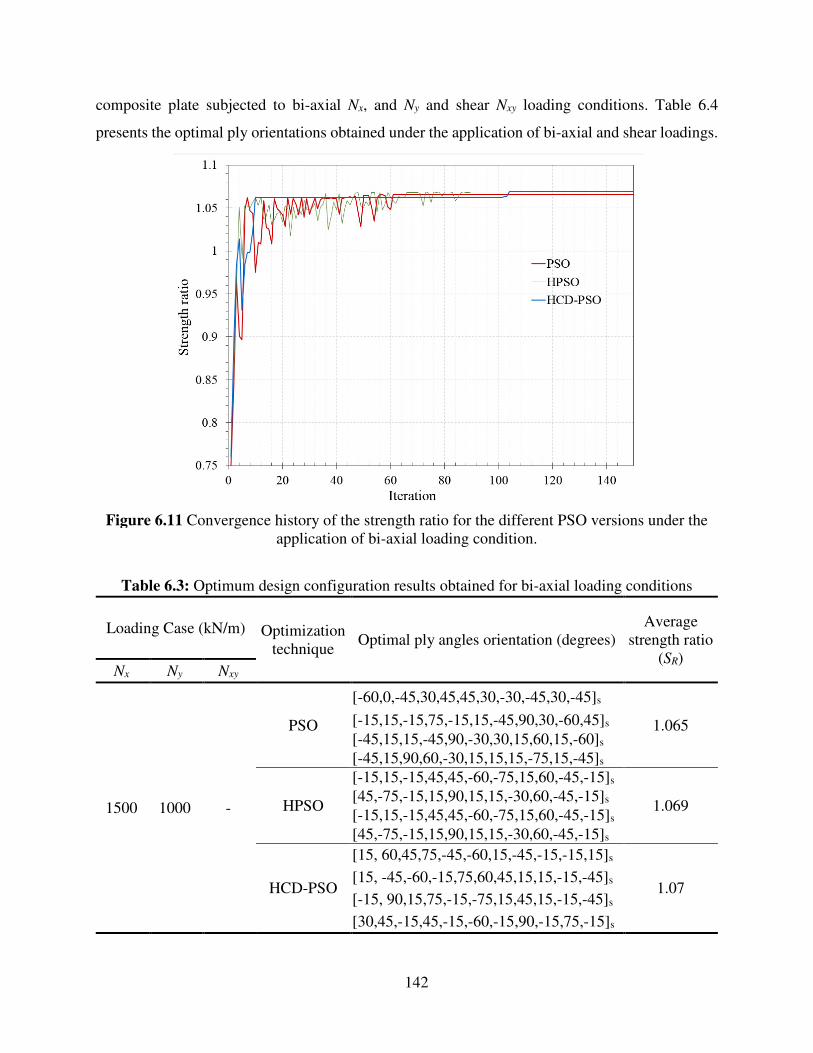
142
composite plate subjected to bi-axial Nx, and Ny and shear Nxy loading conditions. Table 6.4
presents the optimal ply orientations obtained under the application of bi-axial and shear loadings.
Figure 6.11 Convergence history of the strength ratio for the different PSO versions under the application of bi-axial loading condition.
Table 6.3: Optimum design configuration results obtained for bi-axial loading conditions
Loading Case (kN/m) Optimization technique
Optimal ply angles orientation (degrees) Average
strength ratio (SR)
Nx Ny Nxy
1500 1000 -
PSO
[-60,0,-45,30,45,45,30,-30,-45,30,-45]s
1.065 [-15,15,-15,75,-15,15,-45,90,30,-60,45]s
[-45,15,15,-45,90,-30,30,15,60,15,-60]s
[-45,15,90,60,-30,15,15,15,-75,15,-45]s
HPSO
[-15,15,-15,45,45,-60,-75,15,60,-45,-15]s
1.069 [45,-75,-15,15,90,15,15,-30,60,-45,-15]s [-15,15,-15,45,45,-60,-75,15,60,-45,-15]s [45,-75,-15,15,90,15,15,-30,60,-45,-15]s
HCD-PSO
[15, 60,45,75,-45,-60,15,-45,-15,-15,15]s
1.07 [15, -45,-60,-15,75,60,45,15,15,-15,-45]s
[-15, 90,15,75,-15,-75,15,45,15,-15,-45]s
[30,45,-15,45,-15,-60,-15,90,-15,75,-15]s
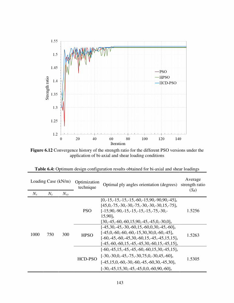
143
Figure 6.12 Convergence history of the strength ratio for the different PSO versions under the application of bi-axial and shear loading conditions
Table 6.4: Optimum design configuration results obtained for bi-axial and shear loadings
Loading Case (kN/m) Optimization technique
Optimal ply angles orientation (degrees) Average
strength ratio (SR)
Nx Ny Nxy
1000 750 300
PSO
[0,-15,-15,-15,-15,-60,-15,90,-90,90,-45]s
1.5256 [45,0,-75,-30,-30,-75,-30,-30,-30,15,-75]s
[-15,90,-90,-15,-15,-15,-15,-75,-30,-15,90]s [30,-45,-60,-60,15,90,-45,-45,0,-30,0]s
HPSO
[-45,30,-45,-30,-60,15,-60,0,30,-45,-60]s
1.5263 [-45,0,-60,-60,-60,-15,30,30,0,-60,-45]s [-60,-45,-60,-45,30,-60,15,-45,-45,15,15]s [-45,-60,-60,15,-45,-45,30,-60,15,-45,15]s
HCD-PSO
[-60,-45,15,-45,-45,-60,-60,15,30,-45,15]s
1.5305 [-30,-30,0,-45,-75,-30,75,0,-30,45,-60]s
[-45,15,0,-60,-30,-60,-45,-60,30,-45,30]s [-30,-45,15,30,-45,-45,0,0,-60,90,-60]s
144
6.5 HCD-PSO APPLICATION ON COMPOSITE CORE DECKS
The designed core web laminate of core A1-HC-W was of [01, ±451]S and [02, ±451]S fiber
architect for the honeycomb sides and the vertical filler web between honeycombs, respectively.
For core A2-HC-CP the web laminate fiber architect was of [±452, 02, ±452]T angles orientation.
This conventional design of core web laminates provides an average strength ratio of 2.203 and
1.305 for the cores A1-HC-W and A2-HC-CP, respectively, due to the application of an in-plane
compressive load only, in which it would results in an expected compressive capacity of 18872
kPa (2737 psi) and 12060 (1749 psi) for both cores, respectively, as previously described in
Chapter 5. For a field application, a practical assumption is to consider the different loading
conditions subjected on the web laminate at the same time during a vehicle crossing as described
in Section 6.2.1. Therefore, the designed composite laminate will achieve a realistic strength ratio
that is capable of providing the code provisions of safety factor and an acceptable margin of safety.
For instance, a web laminate of core A1-HC-W at the location just near the bridge support is
subjected to a combined loading of shear Nxy and compression Nx as presented in Table 6.2. By
recalculating the strength ratio of the core web laminate subjected to these loadings, an average
value of 1.86 strength ratio is achieved from failure analysis using Tsai-Wu and Maximum Stress
failure criteria, similarly the web core laminate subjected to a compressive bi-axial loading at the
mid-span location of the bridge would achieve an average strength ratio of 1.264, which may
significantly affect the compliance with code provisions for a recommended safety factor.
Therefore, a strength design optimization is exigent.
The developed discrete HCD-PSO is applied for the strength design optimization of cores A1-
HC-W and A2-HC-CP considering the loading cases presented in Table 6.2. Table 6.5 illustrates
the optimal ply angles orientation and the obtained strength ratio correspondingly per each loading
case. Figure 6.13 presents the convergence history of the optimum strength ratio achieved for cores
A1-HC-W and A2-HC-CP while applying each loading condition.
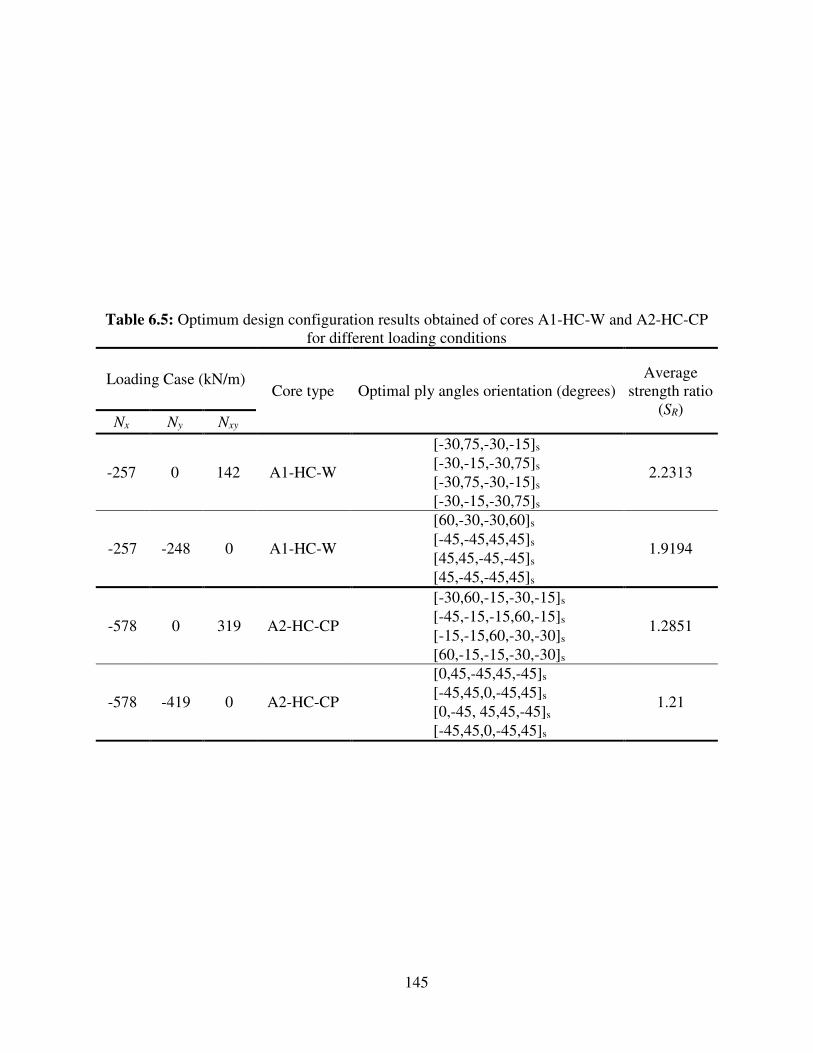
145
Table 6.5: Optimum design configuration results obtained of cores A1-HC-W and A2-HC-CP for different loading conditions
Loading Case (kN/m) Core type Optimal ply angles orientation (degrees)
Average strength ratio
(SR) Nx Ny Nxy
-257 0 142 A1-HC-W
[-30,75,-30,-15]s
2.2313 [-30,-15,-30,75]s
[-30,75,-30,-15]s [-30,-15,-30,75]s
-257 -248 0 A1-HC-W
[60,-30,-30,60]s
1.9194 [-45,-45,45,45]s [45,45,-45,-45]s [45,-45,-45,45]s
-578 0 319 A2-HC-CP
[-30,60,-15,-30,-15]s
1.2851 [-45,-15,-15,60,-15]s
[-15,-15,60,-30,-30]s [60,-15,-15,-30,-30]s
-578 -419 0 A2-HC-CP
[0,45,-45,45,-45]s
1.21 [-45,45,0,-45,45]s
[0,-45, 45,45,-45]s
[-45,45,0,-45,45]s
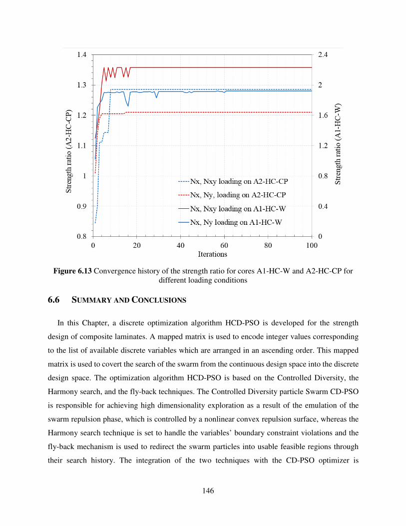
146
Figure 6.13 Convergence history of the strength ratio for cores A1-HC-W and A2-HC-CP for different loading conditions
6.6 SUMMARY AND CONCLUSIONS
In this Chapter, a discrete optimization algorithm HCD-PSO is developed for the strength
design of composite laminates. A mapped matrix is used to encode integer values corresponding
to the list of available discrete variables which are arranged in an ascending order. This mapped
matrix is used to covert the search of the swarm from the continuous design space into the discrete
design space. The optimization algorithm HCD-PSO is based on the Controlled Diversity, the
Harmony search, and the fly-back techniques. The Controlled Diversity particle Swarm CD-PSO
is responsible for achieving high dimensionality exploration as a result of the emulation of the
swarm repulsion phase, which is controlled by a nonlinear convex repulsion surface, whereas the
Harmony search technique is set to handle the variables’ boundary constraint violations and the
fly-back mechanism is used to redirect the swarm particles into usable feasible regions through
their search history. The integration of the two techniques with the CD-PSO optimizer is

147
comprehensively described. The algorithm convergence rate was evaluated on a composite
laminate plate and the results are compared with the performance of developed PSO, and HPSO
discrete versions. The HCD-PSO showed an efficient convergence rate evolving a smooth search
in hyperspace. Therefore, it is concluded that the technique is an efficient candidate for the discrete
optimization of large-scale composite structures. An effective performance evaluation of
composite cores may need specific laboratory tests that are difficult to be setup, for instance
experimentally testing a composite core under multiple loading conditions such as bi-axial and
shear forces cannot be represented expect when a scaled bridge beam is tested. A multiple loading
application on a composite laminate plate may affect in decreasing or increasing the strength ratio
based on the designed fiber orientation compared with a laminate plate subjected to a single
loading. Therefore, the design of the composite core shall comply with these loading combinations
which would results in variety of potential designs with different strength ratios. As a result, HCD-
PSO is applied for the strength design optimization of the core web laminates under multiple
loading conditions in order to ensure a high strength ratio that would meet the design provisions
of specific safety factors and acceptable margins of safety at the critical locations of the bridge
composite structure. The HCD-PSO achieved an increase in the strength ratio of core A1-CH-W
from 1.86 to 2.23 under the application of compressive and shear loading at the location just near
the bridge support, whereas, a strength ratio of 1.91 was obtained with an increase of 1.5 times of
the conventional design under the application of bi-axial compressive loading at the bridge mid-
span.
148
CHAPTER 7
Summary, Conclusions and future work
This research has proposed the Controlled Diversity Particle Swarm Optimizer (CD-PSO) as
an efficient tool for the minimum weight/capacity ratio design of deployable bridge structures, the
study described the development and testing of two sandwich composite cores which are compared
with the balsa core system of the Composite Assault Bridge (CAB) and other two composite
webbed cores that were part of core alternatives for decking the Composite Joint Assault Bridge
(CJAB). Finally, the discrete Heuristic Controlled Diversity Particle Swarm Optimizer (HCD-
PSO) for the maximum strength design of composite laminated plate was developed.
7.1 OPTIMIZATION OF DEPLOYABLE BRIDGES
Based on the wide range of optimization techniques used effectively for structural design
optimization. The performance of selective algorithms of this research study case was assessed,
these algorithms are: Particle Swarm Optimizer (PSO) and Genetic Algorithm (GA) from
heuristic-based algorithms, and First-Order Method (FO) and Zero-Order Method (ZO) from
gradient-based algorithms. The PSO was the suitable technique to achieve rapid convergence rate,
better solutions and competitive computational time.
A comprehensive investigation was conducted of PSO advantages and disadvantages. Further,
the CD-PSO has been developed to cope the possibility of falling in local minima which considered
as the major drawback of PSO. The algorithm implemented a novel technique for better emulation
of the swarm attraction and repulsion, such that the swarm diversity in exploring the design space
behaves in an oscillating wave manner. An assessment of CD-PSO on different truss benchmark
structures was performed, the results were compared with wide range of available results in the
7
149
literature and the robustness of CD-PSO solutions was proved. The new algorithm was applied
another time for the minimum weight/capacity ratio design of the deployable bridge implementing
size and shape optimization. An enhanced normalized weight/capacity ratio of 66.795 percent with
the conventional design was achieved compared with PSO and GA and having 5.35 and 2.01
percent difference, respectively. Moreover, the CD-PSO was hybridized with the Response
Surface Methodology (RSM) in order to outfit the algorithm with a tool to handle complex
structural models such as deployable bridges, where large number of design parameters is
considered and the relationship between these design parameters and the design objective cannot
be easily known. The Hybridized algorithm (CD-PSO + RSM) proved its effectiveness in
distinguishing the significance of design parameters on the design objective. This helped in
evolving the search for better solutions and a best minimum weight/capacity ratio of 65.69 was
achieved.
7.2 COMPOSITE DEPLOYABLE BRIDGE DECKS
Because of the high weight percentage representation of decks in the deployable bridge
design, the current study investigated deck core alternatives to the currently in-service composite
cores, such that the decks represents more than 20% of the metallic deployable bridges weight,
and about 40% of the composite deployable bridges weight. This research proposed two composite
cores alternatives to the balsa system of the CAB deployable bridge and the composite webbed
cores of the CJAB deployable bridge. The composite cores A1-HC-W and A2-HC-CP structural
shape were designed based on different configurations assembly of honeycomb foam beams
wrapped with FRP. The two core systems C4-TC and C5-CC of the webbed cores in the Literature
were reproduced using the same material of the current study to set a baseline of the performance
assessment. In a comparison with the balsa core, both proposed cores in this study achieved similar
shear strength, and exceed the balsa core shear strength-to- areal weight ratio with at least 1.5 times
for the core A2-HC-CP which has the lesser value of the two proposed systems. A progressive
failure FE simulation was conducted and it was found with a good agreement with the proposed
cores failure mode, shear capacity, deflection, and strains, which can be considered a viable tool
for further fatigue simulation of the bridge deck and structure.
150
Despite the premature failure observed in the proposed cores compressive strength test, they
obtained a satisfactory compressive strength capacity that complied with the TDTC code provision
of achieving 1.8 safety factor of the design compressive load. Moreover, they provided a margin
of safety more than 2.2 under the application of a tracked vehicle load of 100 tons (MLC100).
However, core A2-HC-CP achieved similar compressive strength/areal weight ratio with the balsa
system, whereas, core A1-HC-W exceed the balsa performance with 1.44 times. The progressive
failure FE modeling showed a good agreement with the experimental test results which was very
efficient is studying the premature failure mode observed.
The experimentally tested compressive performance of the proposed cores was compared
with the reproduced webbed core systems C4-TC and C5-CC. both cores achieved better
compressive strength and compressive strength to areal weight ratios than core C5-CC, and less
than C4-TC. A design recommendation was set to prevent the premature failure occurred and to
reach the analytically calculated compressive capacity, it is expected to exceed the compressive
capacity of all composite cores presented in the literature after satisfying this design
recommendation.
It is worth noted that, the balsa system as well as the webbed core systems in literature were
manufactured using carbon fiber materials and epoxy formulation that are specially used in
aerospace industry which reflected on the super mechanical properties achieved such as 386 MPa
of shear strength, whereas the proposed cores were fabricated using carbon fiber materials and
epoxy formulation used commonly in the construction industry that resulted in nearly 35 MPa of
shear strength. Given this, the proposed cores are promoted for decking civilian bridges as well
with a relatively lower cost as opposed to currently developed cores for the CAB and CJAB
deployable bridges. In addition, it was shown that weight saving of 14% to 20% can be realized in
the CAB deployable bridge by replacing the balsa deck system with the proposed cores A1-HC-
W and A2-HC-CP, respectively.
7.3 STRENGTH DESIGN OPTIMIZATION OF COMPOSITE CORES
A composite sandwich core is subjected to multiple loading conditions at the same time
during a vehicle passing load along a deployable bridge span. Assessing a sandwich core
performance is very complex under multiple loading conditions in laboratory tests except for a
151
scaled or full structural bridge model which in turn found to be very expensive. On the other hand,
achieving an effective design of composite laminates subjected to multiple loadings is difficult
while the stacking sequence has to be chosen from a wide range of permissive ply orientations in
order to reach the recommended strength and ensure the prevention of failure. Therefore,
increasing the strength ratio of any laminated structure subjected to multiple loading conditions
using the mathematical optimization is exigent and found to be a natural tool. The design
optimization using the developed CD-PSO algorithm was applied for the maximum strength
design of proposed sandwich cores. A discrete version of the CD-PSO was created in order to
introduce a practical design of composite laminated plates. The implemented stress and strain
analysis theory of composites was briefly described, and the failure analysis criterion used as for
the strength design of the composite cores was clarified. The discrete CD-PSO was outfitted with
the Harmony search technique and the fly-back mechanism to handle the constraints violation and
named HCD-PSO. This algorithm integration showed a good convergence rate when tested on a
composite laminated plate subjected to different in-plane loading conditions. Further, the HCD-
PSO was applied for increasing the strength ratio of the proposed cores web laminate while
subjected to multiple loading conditions. The results showed an increase in the strength ratio of
both cores, such that core A1-HC-W strength ratio increased by 1.2 and 1.5 under the application
of axial and shear loading at location just near the bridge support, and bi-axial loading at the bridge
mid-span, respectively.
7.4 CONTRIBUTIONS
The contributions of this research study can be summarized as follows:
• An efficient controlled diversity particle swarm optimizer CD-PSO with robust stability is
developed for the structural design optimization through a better emulation of the attraction
and repulsion phenomenon of swarm of birds.
• An efficient hybrid CD-PSO optimizer with RSM for the optimal design of large-scale
structures and deployable bridges is proposed, the performance of the methodology was
assessed with classical PSO and GA and showed better solution, and rapid convergence.
• Novel Light weight with high shear and compressive strength composite core decks are
developed for decking the deployable bridges of high carrying capacity of 100 tons. Both
cores showed higher performance in terms of strength to areal core weight ratio when
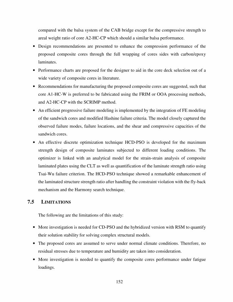
152
compared with the balsa system of the CAB bridge except for the compressive strength to
areal weight ratio of core A2-HC-CP which should a similar balsa performance.
• Design recommendations are presented to enhance the compression performance of the
proposed composite cores through the full wrapping of cores sides with carbon/epoxy
laminates.
• Performance charts are proposed for the designer to aid in the core deck selection out of a
wide variety of composite cores in literature.
• Recommendations for manufacturing the proposed composite cores are suggested, such that
core A1-HC-W is preferred to be fabricated using the FRIM or OOA processing methods,
and A2-HC-CP with the SCRIMP method.
• An efficient progressive failure modeling is implemented by the integration of FE modeling
of the sandwich cores and modified Hashine failure criteria. The model closely captured the
observed failure modes, failure locations, and the shear and compressive capacities of the
sandwich cores.
• An effective discrete optimization technique HCD-PSO is developed for the maximum
strength design of composite laminates subjected to different loading conditions. The
optimizer is linked with an analytical model for the strain-strain analysis of composite
laminated plates using the CLT as well as quantification of the laminate strength ratio using
Tsai-Wu failure criterion. The HCD-PSO technique showed a remarkable enhancement of
the laminated structure strength ratio after handling the constraint violation with the fly-back
mechanism and the Harmony search technique.
7.5 LIMITATIONS
The following are the limitations of this study:
• More investigation is needed for CD-PSO and the hybridized version with RSM to quantify
their solution stability for solving complex structural models.
• The proposed cores are assumed to serve under normal climate conditions. Therefore, no
residual stresses due to temperature and humidity are taken into consideration.
• More investigation is needed to quantify the composite cores performance under fatigue
loadings.

153
• The developed sandwich cores were tested only in a one-way bending, whereas, other tests
are needed to quantify the performance in two-way bending application for the core A2-HC-
CP.
7.6 FUTURE WORK
Based on the findings of this study a second phase is expected to prolong and it will cover
the following scopes:
• The proposed composite cores will be used for decking a deployable bridge system. A
sandwich core will be chosen as a candidate deck to sustain the compression in top of a one-
quarter scale FRP bridge beam.
• Multiple objective discrete optimization will be performed for the minimum weight and cost
design of the whole deployable bridge treadway.
• The flexural performance, safety factors and margins of safety will be evaluated based on
the Trilateral Design and Test Code for Military Bridging and Gap Crossing operations’
requirements. The evaluation will include a moment and shear proof tests by simulating the
axle load distribution of a vehicle using a whiffle tree structure.
• Core A2-HC-CP will be tested for two-way bending application, such that the composite
deck will be manufactured with a dimension covering the treadway suggested width and a
deck length supported on two transverse stiffeners (bulk heads).
• Extend the performance assessment of the proposed cores experimentally against fatigue and
validate the results using a progressive failure modeling.
• Assess the performance of the whole developed and optimized scaled deployable bridge
treadway against fatigue and cyclic loadings experimentally.
• Validate the fatigue performance of the scaled deployable bridge treadway through a
progressive failure modeling.

154
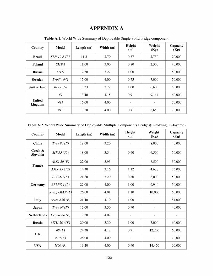
155
APPENDIX A
Table A.1. World Wide Summary of Deployable Single Solid bridge component
Capacity
(Kg)
Weight
(Kg)
Height
(m) Width (m) Length (m) Model Country
20,000 2,750 0.87 2.70 11.2 XLP-10 AVLB Brazil
40,000 2,300 0.80 3.00 11.00 SMT-1 Poland
50,000 - 1.00 3.27 12.30 MTU Russia
50,000 7,000 0.75 4.00 15.00 Brodiv-941 Sweden
50,000 6,600 1.00 3.79 18.23 Bru Pz68 Switzerland
60,000 9,144 0.91 4.18 13.40 #9
United
kingdom 70,000 - - 4.00 16.00 #11
70,000 5,650 0.71 4.00 13.50 #12
Table A.2. World Wide Summary of Deployable Multiple Components Bridges(F=folding, L=layered)
Capacity
(Kg) Weight
(Kg) Height
(m) Width (m) Length (m) Model Country
40,000 8,000 - 3.20 18.00 Type 84 (F) China
50,000 6,500 0.90 3.34 18.00 MT-55 (55) Czech &
Slovakia
50,000 8,500 - 3.95 22.00 AMX-30 (F)
France 25,000 4,630 1.12 3.16 14.30 AMX-13 (13)
50,000 6,000 0.80 3.20 21.60 BLG-60 (F)
Germany 50,000 9,940 1.00 4.00 22.00 BRLPZ-1 (L)
60,000 10,000 1.10 4.01 26.00 Krupp-MAN (L)
54,000 - 1.00 4.10 21.40 Astra A26 (F) Italy
40,000 - 0.90 3.50 12.00 Type 67 (F) Japan
- - - 4.02 19.20 Centurion (F) Netherlands
60,000 7,000 1.00 3.30 20.00 MTU-20 (3F) Russia
60,000 12,200 0.91 4.17 24.38 #8 (F)
UK 70,000 - - 4.00 26.00 #10 (F)
60,000 14,470 0.90 4.00 19.20 M60 (F) USA

156
APPENDIX B
Begin; Generate random population of Np Particles; Calculate particles diversity; Initiate swarm diversity control function div.rate; For each particle� ∈ s{, evaluate fitness; Trial=0; Switch=0; If Swarm diversity <div.rate; Switch to repulsion phase; Trial=Trial+1; else; Keep attraction phase; End; Initiate the value of inertia weight w; For each particle: Set Pbest ��(5,�)D as the best position for particle i, If the fitness is better than Pbest; Pbest(i)= fitness(i); End; Set Gbest ��(5,�)E as the best position for all particles; Calculate particle velocity; Check velocity bounds; Update particle position; Check particle encoded parameter bounds; If ��(5,�)E − ��(5,�|�)E < 0.001; Switch=Switch+1; End;
If Trial= �}~:hi OR Switch=�}~:hi;
Initiate RSM analysis; Categorize parameters reference to influence rate; Mutate poor parameter to the Gbest equivalent; Fixing mutated poor parameter value; End; If��(5,�) > ��?;
��(5,�) = ��?; End; If��(5,�) < ��>;
��(5,�) = ��>; End;
Check if termination condition is True; End; End; End;
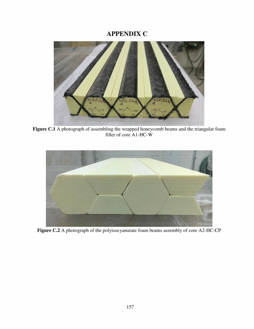
157
APPENDIX C
Figure C.1 A photograph of assembling the wrapped honeycomb beams and the triangular foam
filler of core A1-HC-W
Figure C.2 A photograph of the polyisocyanurate foam beams assembly of core A2-HC-CP
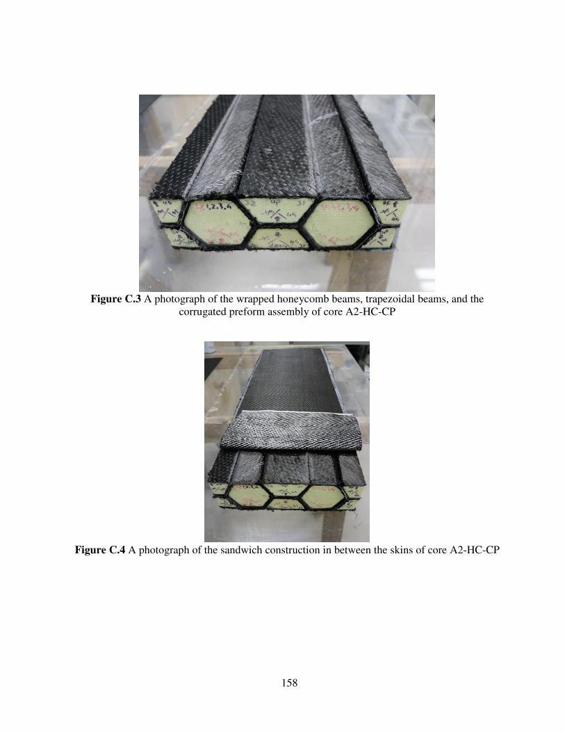
158
Figure C.3 A photograph of the wrapped honeycomb beams, trapezoidal beams, and the
corrugated preform assembly of core A2-HC-CP
Figure C.4 A photograph of the sandwich construction in between the skins of core A2-HC-CP
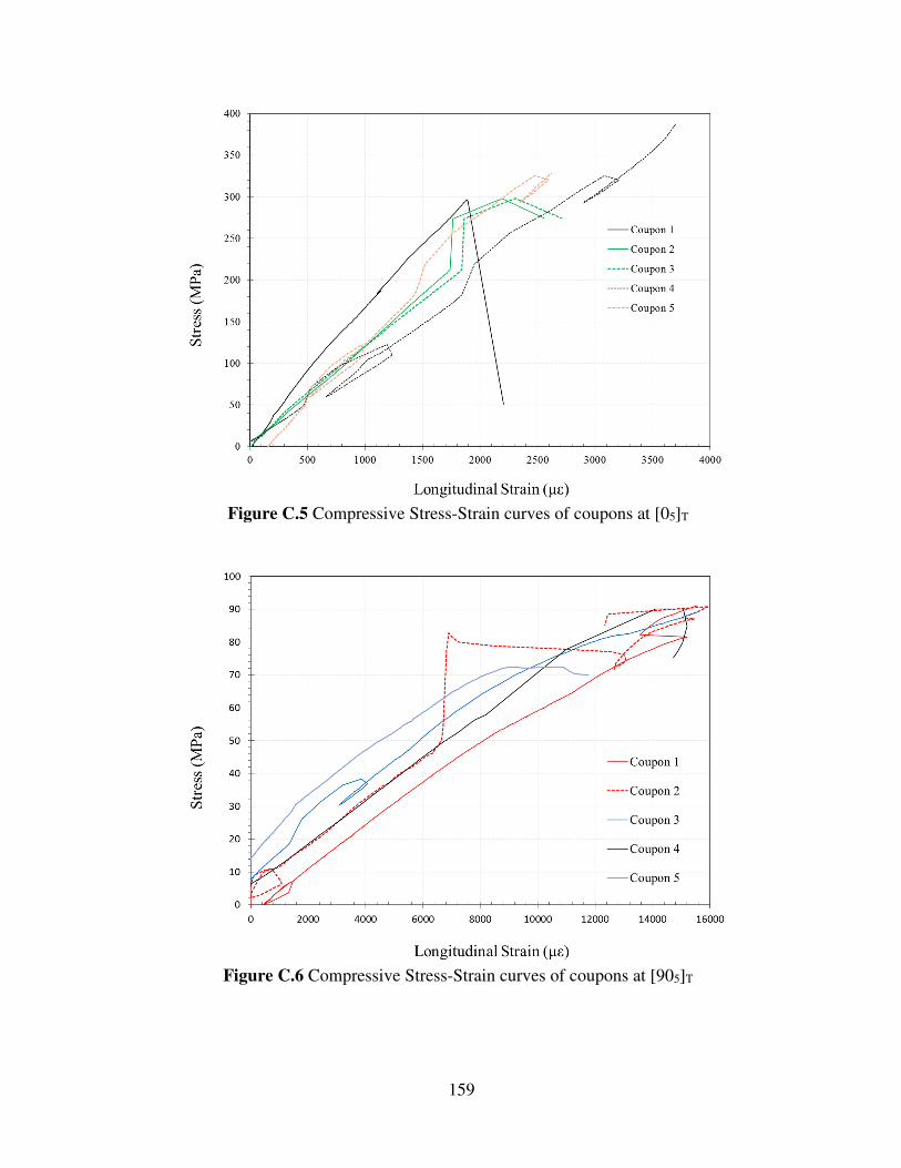
159
Figure C.5 Compressive Stress-Strain curves of coupons at [05]T
Figure C.6 Compressive Stress-Strain curves of coupons at [905]T
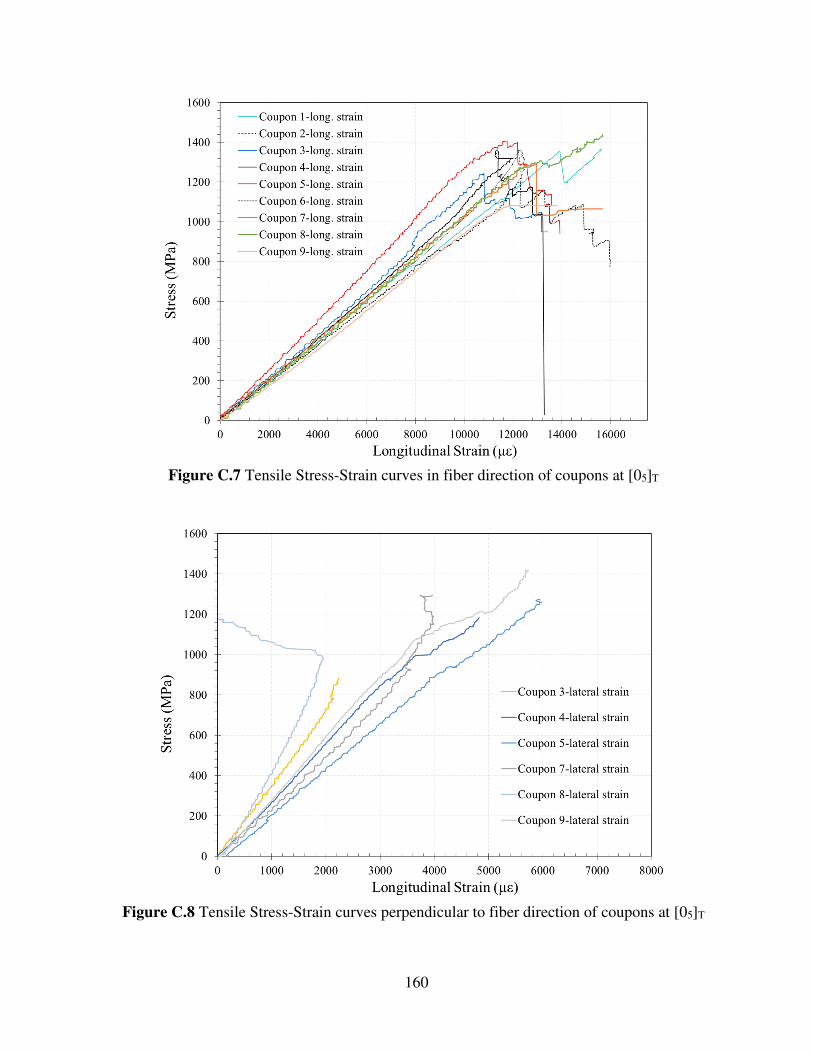
160
Figure C.7 Tensile Stress-Strain curves in fiber direction of coupons at [05]T
Figure C.8 Tensile Stress-Strain curves perpendicular to fiber direction of coupons at [05]T
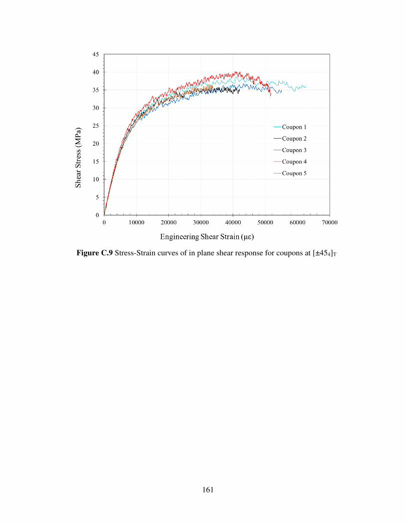
161
Figure C.9 Stress-Strain curves of in plane shear response for coupons at [±454]T
162
REFERENCES
ANSYS, U. M. (1999). Structural Analysis Guide (Version Version 5.6). Ario, I., Chikahiro, Y., and Tanaka, Y. (2011). Dynamic analysis for the prototype of a new type
of Mobilebridge TM. Proceedings of the 7th anuual Europian Nonlinear Dynamic Conference. ENOC 2011. July 2011.
Ario, I., Nakazawa, M., Tanaka, Y., Tanikura, I., and Ono, S. (2013). Development of a prototype deployable bridge based on origami skill. Automation in Construction, 32, 104-111.
Arora, J. (2012). Introduction to optimum design. MA, USA & Oxford, UK: Academic Press. Below, L., Palmer, M., Lindow, D., and Kellogg, D. (2003). Bridging Study: Phase 2. US Army
Maneuver Support Center, Fort Leonard Wood, MO. Bischmann, P. (1985). River Crossing in the Central Region. NATO’s Sixteen Nations, 3, 76. Box, G. E., and Wilson, K. (1951). On the experimental attainment of optimum conditions. Journal
of the Royal Statistical Society. Series B (Methodological), 13(1), 1-45. Brown, R. T., & Zureick, A.-H. (2001). Lightweight composite truss section decking. Marine
Structures, 14(1–2), 115-132. C363, A. (2011). C393/C393M − 11, Standard test method for core shear properties of sandwich
constructions by beam flexure (Vol. 15.03): American Society for Testing and Materials. West Conshohocken, PA.
C364, A. (2012). C394/C394M − 12, Standard Test Method for Edgewise Compressive Strength of Sandwich Constructions (Vol. 15.03): American Society for Testing and Materials. West Conshohocken, PA.
C365, A. (2011). C395/C395M − 11a, Standard Test Method for Flatwise Compressive Properties of Sandwich Cores (Vol. 15.03): American Society for Testing and Materials. West Conshohocken, PA.
Camp, C. (2007). Design of Space Trusses Using Big Bang–Big Crunch Optimization. Journal of Structural Engineering, 133(7), 999-1008.
Camp, C., and Bichon B. (2004). Design of Space Trusses Using Ant Colony Optimization. Journal of Structural Engineering, 130(5), 741-751.
Camp, C., Pezeshk, S., and Cao, G. (1998). Optimized Design of Two-Dimensional Structures Using a Genetic Algorithm. Journal of Structural Engineering, 124(5), 551-559.
Cao, G. (1996). Optimized design of framed structures using a genetic algorithm. Ph.D. Thesis, The University of Memphis, Ann Arbor.
Chechkin, A. V., Metzler, R., Klafter, J., and Gonchar, V. Y. (2008). Introduction to the theory of Lévy flights, Anomalous Transport: Foundations and Applications, pp. 129-162.
Chikahiro, Y., Ario, I., Nakazawa, M., Ono, S., Holnicki-Szulc, J., Pawlowski, P., and Graczykowski, C. (2014). An experimental study on the design method of a real-sized Mobile Bridge for a moving vehicle. Mobile and Rapidly Assembled Structures IV, 136, 93.
163
Cluff, L. (2007). Effects of the 2004 Sumatra-Andaman earthquake and Indian Ocean tsunami in Aceh province. bridge-washington-national academy of engineering, 37(1), 12.
Coker, C. (2009). New Options on Military Bridging. Military Technology, 33(3), 42. Connors, S. C., and Foss, C. F. (2005). Jane's Military Vehicles and Logistics 2005-2006: Jane's
Information Group Limited. Connors, S. C., and Foss, C. F. (2006). Jane's Military Vehicles and Logistics 2005-2006: Jane's
Information Group Limited. Das, S., and Suganthan, P. N. (2011). Differential evolution: A survey of the state-of-the-art.
Evolutionary Computation, IEEE Transactions on, 15(1), 4-31. Davalos, J. F., Qiao, P., Frank Xu, X., Robinson, J., and Barth, K. E. (2001). Modeling and
characterization of fiber-reinforced plastic honeycomb sandwich panels for highway bridge applications. Composite structures, 52(3–4), 441-452.
De Jong, K. A. (1975). Analysis of the behavior of a class of genetic adaptive systems. Ph.D. Thesis. University of Michigan, Ann Arbo.
DiMarco, A. (2004). Bridging the gap: Modernizing Army bridge units. Engineer, Prof. Bull., U.S. Army Maneuver Support Center, 2, 20-21.
Dobbs, M., and Nelson, R. (1976). Application of optimality criteria to automated structural design. AIAA journal, 14(10), 1436-1443.
Eberhart, R. C., and Kennedy, J. (1995). A new optimizer using particle swarm theory. Proceedings of the sixth international symposium on micro machine and human science. New York, NY. 39-43
Eberhart, R. C., and Yuhui, S. (2001). Particle swarm optimization: developments, applications and resources. Proceedings of the 2001 Congress on the Evolutionary Computation.
Elbeltagi, E., Hegazy, T., and Grierson, D. (2005). Comparison among five evolutionary-based optimization algorithms. Advanced Engineering Informatics, 19(1), 43-53.
Eslami, M., Shareef, H., Khajehzadeh, M., and Mohamed, A. (2012). A survey of the state of the art in particle swarm optimization. Research Journal of Applied Sciences, Engineering and Technology, 4(9), 1181-1197.
Fiacco, A. V., and McCormick, G. P. (1990). Nonlinear programming: sequential unconstrained minimization techniques: Siam, (Vol. 4).
Fourie, P., and Groenwold, A. (2002). The particle swarm optimization algorithm in size and shape optimization. Structural and Multidisciplinary Optimization, 23(4), 259-267.
Gellatly, R. A. (1966). development of procedures for large scale automated minimum weight structural design: DTIC Document.
Gellatly, R. A., & Berke, L. (1971). Optimal Structural Design: DTIC Document. Giunta, A. A., Wojtkiewicz, S. F., and Eldred, M. S. (2003). Overview of modern design of
experiments methods for computational simulations. Proceedings of the 41st AIAA aerospace sciences meeting and exhibit, AIAA-2003-0649.
Haklı, H., and Uğuz, H. (2014). A novel particle swarm optimization algorithm with Levy flight. Applied Soft Computing, 23(0), 333-345.
164
Hanus, J., Bank, L., and Oliva, M. (2008). Investigation of a Structural FRP Stay-in-Place Form for a Prototype Military Bridge System. ACI Special Publication, 257, 53-70.
Hashin, Z. (1980). Failure criteria for unidirectional fiber composites. Journal of applied mechanics, 47(2), 329-334.
Hassan, R., Cohanim, B., De Weck, O., and Venter, G. (2005). "A comparison of particle swarm optimization and the genetic algorithm." Proceedings of the 1st AIAA multidisciplinary design optimization specialist conference, 18-21.
Hassan, T., Reis, E. M., and Rizkalla, S. H. (2003). Innovative 3-D FRP sandwich panels for bridge decks. Proceedings of the Fifth Alexandria International Conference on Structural and Geotechnical Engineering.
Haug, E. J., and Arora, J. S. (1979). Applied optimal design: mechanical and structural systems: John Wiley & Sons.
Hetényi, M. (1946). Beams on elastic foundation. The University of Michigan Press;G. Cumberlege, Oxford university press, Ann Arbor; London.
Hoa, S. V. (2009). Principles of the manufacturing of composite materials: DEStech Publications, Inc.
Holland, J. H. (1975). Adaptation in natural and artificial system: an introduction with application to biology, control and artificial intelligence. University of Michigan Press, Ann Arbor.
Jang, S. H., Hwang, I. W., Kwon, B. C., Kim, S. T., and Choi, Y. H. (2012). Structural optimization based on static design criteria of a long span mobile bridge using genetic algorithm. Applied Mechanics and Materials, Trans Tech Publ, 4732-4741.
Karaboga, D. (2005). An idea based on honey bee swarm for numerical optimization: Technical report-tr06, Erciyes university, engineering faculty, computer engineering department.
Kaveh, A. (2014). Chaos Embedded Metaheuristic Algorithms Advances in Metaheuristic Algorithms for Optimal Design of Structures: Springer International Publishing. pp. 369-391.
Kaveh, A., and Ghazaan, M. I. (2014). Enhanced colliding bodies optimization for design problems with continuous and discrete variables. Advances in Engineering Software, 77, 66-75.
Kaveh, A., and Khayatazad, M. (2012). A new meta-heuristic method: Ray Optimization. Computers & structures, 112–113, 283-294.
Kaveh, A., Sheikholeslami, R., Talatahari, S., and Keshvari-Ilkhichi, M. (2014). Chaotic swarming of particles: A new method for size optimization of truss structures. Advances in Engineering Software, 67(0), 136-147.
Kaveh, A., and Talatahari, S. (2009a). "Hybrid algorithm of harmony search, particle swarm and ant colony for structural design optimization. Harmony search algorithms for structural design optimization, Springer, Berlin Heidelberg, 159-198.
Kaveh, A., and Talatahari, S. (2009b). Size optimization of space trusses using Big Bang–Big Crunch algorithm. Computers and Structures, 87(17), 1129-1140.
165
Keller, T., and Gürtler, H. (2005). Quasi-static and fatigue performance of a cellular FRP bridge deck adhesively bonded to steel girders. Composite Structures, 70(4), 484-496.
Keller, T., Rothe, J., De Castro, J., and Osei-Antwi, M. (2013). GFRP-balsa sandwich bridge deck: Concept, design, and experimental validation. Journal of Composite for Construction, 18(2), 04013043.
Kermanidis, T., Labeas, G., Tserpes, K., and Pantelakis, S. (2000). "Finite element modeling of damage accumulation in bolted composite joints under incremental tensile loading." Proceedings of the Third ECCOMAS Congress, 11-14.
kerr, j. v. (1990). "U.S.-German cooperative efforts in military bridging." Army RD&A Bulletin, Headquarters Department of U.S. army, USA, 1-4.
Khan, M., Willmert, K., & Thornton, W. (1979). An optimality criterion method for large-scale structures. AIAA journal, 17(7), 753-761.
Koehler, J., and Owen, A. (1996). "9 Computer experiments." Handbook of Statistics, 13 261-308. Kosmatka, J. (2011). Composite bridging for military and emergency applications. 8th annual
proceeding, Annual Int. Conf. on Composites/Nano Engineering. Kosmatka, J. B., Grippo, W., Policelli, F., Charbonnet, S., Randolph, B., and Hegimier, G. (2000).
Advanced composites for bridge infra-structure renewal- phase II DARPA: University of California San Diego. pp. 326.
Kovács, G., and Spens, K. M. (2007). Humanitarian logistics in disaster relief operations. International Journal of Physical Distribution & Logistics Management, 37(2), 99-114.
Koza, J. R. (1992). Genetic programming: on the programming of computers by means of natural selection: MIT press. Vol. 1.
Koziel, S., and Yang, X. (2011). Computational optimization, methods and algorithms. Springer. Vol. 356.
Kutner, M. H., Nachtsheim, C. J., Neter, J., and Wasserman, W. (2004). Applied linear regression models. McGraw-Hill Irvin.
Landherr, J. (2008). Dynamic analysis of a FRP deployable box beam. Lederman, G., You, Z., and Glišić, B. (2014). A novel deployable tied arch bridge. Engineering
Structures, 70(0), 1-10. Lee, K. S., and Geem, Z. W. (2004). A new structural optimization method based on the harmony
search algorithm. Computers & structures, 82(9–10), 781-798. Li, L. J., Huang, Z. B., and Liu, F. (2009). A heuristic particle swarm optimization method for
truss structures with discrete variables. Computers and structures, 87(7–8), 435-443. Li, N., & Li, Y. X. (2012). A Diversity Guided Particles Swarm Optimization. Advanced Materials
Research, Trans Tech Publ, 532, 1429-1433. Link, C. (2003). Development of panel-to-panel connection for use with a pultruded fiber-
reinforced-polymer bridge deck system. Civil & Environmental Engineering. Blacksburg, Virginia Polytechnic Institute & State University. MS.
Liu, Z. (2007). Testing and analysis of a fiber-reinforced polymer (FRP) bridge deck. Virginia Polytechnic Institute and State University.
166
Lopez-Anido, R., Ganga Rao, H. V., Vedam, V., and Overby, N. (1997). Design and evaluation of a modular FRP bridge deck. marketing technical regulatory sessions of the composites institutes international composites expo, 3-Edition.
Luh, G.-C., and Lin, C.-Y. (2008). Optimal design of truss structures using ant algorithm. Structural and Multidisciplinary Optimization, 36(4), 365-379.
Luh, G.-C., and Lin, C.-Y. (2011). Optimal design of truss-structures using particle swarm optimization. Computers & structures, 89(23–24), 2221-2232.
M. Dorigo, and Caro, G. D. (1999, 1999). Ant colony optimization: a new meta-heuristic. Proceedings of the 1999 Congress on Evolutionary Computation. Washington, DC., pp. 1470–1477.
Mukhopadhyay, T., Dey, T. K., Dey, S., and Chakrabarti, A. (2015). Optimisation of Fibre-Reinforced Polymer Web Core Bridge Deck—A Hybrid Approach. Structural Engineering International, 25(2), 173-183.
Myers, R. H., Montgomery, D. C., and Anderson-Cook, C. (2009). Response surface methodology: product and process optimization using designed experiments: John Wiley & Sons, New York.
Navy, U. S. (2005). US Navy 050127-N-0057P-268 tsunami rescue effort near Banda Aceh, Sumatra, Indonesia,. from https://commons.wikimedia.org/wiki/File:US_Navy_050127-N-0057P-268
NOAA. (1998). Mitch: The Deadliest Atlantic Hurricane Since 1780. Retrieved Sept. 30, 2014, from http://www.ncdc.noaa.gov/oa/reports/mitch/mitch.html
Nor, N. M. (2011). Simulation analysis of a foldable carbon fiber reinforced polymer bridge prototype. National Postgraduate Conference (NPC), IEEE, 1-4.
Nor, N. M., Agusril, S., Alias, M. Y., Mujahid, A. A. Z., and Shohaimi, A. (2012). Dynamic Analysis of Sandwiched Composite Foldable Structure under Heavy Vehicle Load. Applied Mechanics and Materials, Trans Tech Publ, 110, 2331-2336.
Osei-Antwi, M., de Castro, J., Vassilopoulos, A. P., & Keller, T. (2013). FRP-balsa composite sandwich bridge deck with complex core assembly. Journal of Composites for Construction, 17(6).
Osman, A. (2006). Optimum Design or Orthotropic Metallic Deck Bridges. M. Sc. Thesis, Military Technical College, Egypt.
Pant, M., Radha, T., and Singh, V. P. (2007). A Simple Diversity Guided Particle Swarm Optimization. IEEE Congress on the Evolutionary Computation. CEC 2007.
Paulo, R. (1976). optimization of multi-constrained structures based on optimality criteria. 17th Structures, Structural Dynamics, and Materials Conference: American Institute of Aeronautics and Astronautics.
Perez, R. E., and Behdinan, K. (2007). Particle swarm approach for structural design optimization. Computers and structures, 85(19–20), 1579-1588.
167
Poloni, C., Pediroda, V., Clarich, A., and Steven, G. (2002). The use of Design of Experiments (DOE) and Response Surface Analysis (RSA) in PSO. Product and System Optimization (PSO) (pp. 3). Copenhagen.
Repetski, E. J. (2003). Assessment of Bridging Requirements and Current Bridging Capabilities for use of Legacy Heavy Forces Inside the Contemporary Operational Environment: DTIC Document.
Reyes-Sierra, M., and Coello, C. C. (2006). Multi-objective particle swarm optimizers: A survey of the state-of-the-art. International journal of computational intelligence research, 2(3), 287-308.
Riget, J., and Vesterstrøm, J. S. (2002). A diversity-guided particle swarm optimizer-the ARPSO. Dept. Comput. Sci., Univ. of Aarhus, Aarhus, Denmark, Tech. Rep, 2, 2002.
Robinson, M., and Kosmatka, J. (2010). Experimental dynamic response of a short-span composite bridge to military vehicles. Journal of Bridge Engineering, 16(1), 166-170.
Robinson, M., and Kosmatka, J. (2008a). Development of a Short-Span Fiber-Reinforced Composite Bridge for Emergency Response and Military Applications. Journal of Bridge Engineering, 13(4), 388-397.
Robinson, M., and Kosmatka, J. (2008b). Light-weight fiber-reinforced polymer composite deck panels for extreme applications. Journal of Composites for Construction, 12(3), 344-354.
Robinson, M. J. (2008). Simulation of the vacuum assisted resin transfer molding (VARTM) process and the development of light-weight composite bridging. PhD Thesis, UCSD, San Diego, California.
Russell, B. R., and Thrall, A. P. (2012). Portable and rapidly deployable bridges: Historical perspective and recent technology developments. Journal of Bridge Engineering, 18(10), 1074-1085.
Saatcioglu, M., Ghobarah, A., and Nistor, I. (2006). Performance of structures in Indonesia during the December 2004 great Sumatra earthquake and Indian Ocean tsunami. Earthquake Spectra, 22(S3), 295-319.
Santner, T. J., Williams, B. J., and Notz, W. I. (2013). The design and analysis of computer experiments: Springer Science & Business Media.
Schmit, L. A., and Farshi, B. (1974). Some approximation concepts for structural synthesis. AIAA journal, 12(5), 692-699.
Schmit, L. A., and Miura, H. (1976). Approximation concepts for efficient structural synthesis: US National Aeronautics and Space Administration. NASA Contractor Report, 2552
Schutte, J. F., and Groenwold, A. A. (2003). Sizing design of truss structures using particle swarms. Structural and Multidisciplinary Optimization, 25(4), 261-269.
Shi, Y. (2001). Particle swarm optimization: developments, applications and resources. IEEE Proceedings of the Congress on evolutionary computation, 81-86.
Shi, Y., and Eberhart, R. (1998). A modified particle swarm optimizer. Evolutionary Computation Proceedings, The 1998 IEEE World Congress on Computational Intelligence. 69-73.
168
Shokrieh, M., Lessard, L., & Poon, C. (1996). Three-dimensional progressive failure analysis of pin/bolt loaded composite laminates. The AGARD Conference Proceedings, Neuilly-Sur-Seine, France.
Siegel, R. A. (2000). America's Grand Strategy Choices: DTIC Document. Tanweer, M. R., Suresh, S., and Sundararajan, N. (2015). Self regulating particle swarm
optimization algorithm. Information Sciences, 294(0), 182-202. Thomas, A. S., and Kopczak, L. R. (2005). From logistics to supply chain management: the path
forward in the humanitarian sector. Fritz Institute, 15, 1-15. Thomas, G. R., and Sia, B. J. (2013). A Rapidly Deployable Bridge System Structures Congress
2013: Bridging Your Passion with Your Profession, ASCE, 656-667. Trilateral Design and Test Code For Military Bridging and Gap Crossing Equipment. (May 2005):
Trilateral Design and Analysis Group of the United States, Federal Republic of Germany and the United Kingdom of Great Britain.
Tuwair, H., Volz, J., ElGawady, M., Mohamed, M., Chandrashekhara, K., and Birman, V. (2015). Testing and Evaluation of Polyurethane-Based GFRP Sandwich Bridge Deck Panels with Polyurethane Foam Core. Journal of Bridge Engineering, 0(0).
Venkayya, V. (1971). Design of optimum structures. Computers and structures, 1(1), 265-309. Venkayya, V., Khot, N., and Reddy, V. (1968). Optimization of structures based on the study of
energy distribution: DTIC Document. Wight, R., Erki, M., Shyu, C., Tanovic, R., and Heffernan, P. (2006). Development of FRP short-
span deployable bridge-Experimental results. Journal of Bridge Engineering, 11(4), 489-498.
Williams;, B., Shehata;, E., and Rizkalla, S. H. (2003). Filament-Wound Glass Fiber Reinforced Polymer Bridge Deck Modules. Journal of Composites for Construction, 7(3), 266-273.
Winney, M. (1994). On active service. New Civil Engineer (1077), Page. 1-20. Xia, R., and Liu, P. (1987). Structural optimization based on second-order approximations of
functions and dual theory. Computer Methods in Applied Mechanics and Engineering, 65(2), 101-114.
Xie, A. Y. (2007). Development of an FRP deployable bridge. M. Sc.Thesis, Royal Military College of Canada (Canada), Ann Arbor.
Yin, S., Lin, J., and Huang, P. (2013). Studies on new forms of portable bridges for disaster relief. Proceedings of the Thirteenth East Asia-Pacific Conference on Structural Engineering and Construction (EASEC-13), the Thirteenth East Asia-Pacific Conference on Structural Engineering and Construction (EASEC-13), G-3-2.
Yuhui, S., and Eberhart, R. (1998). A modified particle swarm optimizer. Procedings on the Evolutionary Computation, 1998.
Zetterberg, T., Åström, B. T., Bäcklund, J., and Burman, M. (2001). On design of joints between composite profiles for bridge deck applications. Composite structures, 51(1), 83-91.
169
Zhang, D., Zhao, Q., Huang, Y., Li, F., Chen, H., and Miao, D. (2014). Flexural properties of a lightweight hybrid FRP-aluminum modular space truss bridge system. Composite structures, 108, 600-615.
Zhou, A. (2002). Stiffness and Strength of Fiber Reinforced Polymer Composite Bridge Deck Systems. Ph.D. Thesis, Faculty of the Virginia Polytechnic Institute and State University, Blacksburg, Virginia, USA.
Zhou, A., Coleman, J. T., Temeles, A. B., Lesko, J. J., and Cousins, T. E. (2005). Laboratory and field performance of cellular fiber-reinforced polymer composite bridge deck systems. Journal of Composites for Construction, 9(5), 458-467.
Zhou, A., Qu, B.-Y., Li, H., Zhao, S.-Z., Suganthan, P. N., and Zhang, Q. (2011). Multiobjective evolutionary algorithms: A survey of the state of the art. Swarm and Evolutionary Computation, 1(1), 32-49.
Zhou, M., and Rozvany, G. (1993). DCOC: an optimality criteria method for large systems Part II: algorithm. Structural optimization, 6(4), 250-262.
Zhu, J., and Lopez, M. M. (2014). Performance of a lightweight GFRP composite bridge deck in positive and negative bending regions. Composite structures, 113(0), 108-117.
WEBSITES
Web-1:http://firstpeoples.org/wp/over-3-million-affected-by-massive-philippines-earthquake/, consulted 5 July 2015.
Web-2: http://newsinfo.inquirer.net/510343/11-bridges-in-bohol-reopened-to-traffic, consulted 5 Aug 2015
Web-3:http://home.hiroshima-u.ac.jp/bridge2/out-hiro/open/2009-sayo/sayo-shiso-flownbridges2.pdf, consulted 5 Aug. 2015
Web-4: https://www.wfel.com/downloads/wfel-mgb-brochure.pdf, consulted 5 Aug. 2015
Web-5: https://www.wfel.com/downloads/wfel-dsb-brochure.pdf, consulted 5 Aug. 2015


