Determinants of School Attendance in IndianVillages: Do contextual effects matter?∗

Benoit Dostie†and Rajshri Jayaraman‡

October 29, 2003

Abstract

Attaining universal primary school education remains an elusive goalin many developing countries. Previous explorations of schooling decisionshave focused primarily on micro determinants. However, anecdotal evi-dence suggests that contextual effects at the village level may also be im-portant. In this paper, we explore the effect of village level characteristicson school attendance by formalising the anecdotal evidence, controllingfor unobserved correlated effects and endogeneity, using a recent surveyfrom two North Indian states. We find that various village-level influencesmatter in the school attendance decision. However, results depend impor-tantly upon whether or not one corrects for unobserved heterogeneity.

JEL classification: I21, O12.Keywords: Education, Contextual effects, Probit, Random effects, Endo-

geneity, Social Capital, India.

∗The authors would like to thank seminar participants at NYU, Laval, Sherbrooke and theUniversity of Munich for useful comments and suggestions.

†Institute of Applied Economics, HEC Montréal, 3000, chemin de la Côte-Sainte-Catherine,Montréal, H3T 2A7. benoit.dostie@hec.ca

‡Center for Economic Studies, University of Munich, Schackstrasse 4, 80539 Munich, Ger-many. jayaraman@cesifo.de

1

1 Introduction

Universal primary school education has long been a goal of governments in

developing countries. Despite making enormous strides in increasing school at-

tendance over the last 50 years this goal remains elusive for many of them.1 This

is troubling given the importance of basic education as an input into economic

and social development.

In India, the constitution of 1950 urged states to provide “free and compul-

sory education for all children until they complete the age of fourteen years”

by 1960.2 By the early 1990s, however, one-third of children were estimated

to be out of school. Alarming in and of itself, this proportion rises to almost

one-half in the large north Indian states which account for over 40 per cent of

the country’s population.3

Why do so many children fail to attend school? The simple answer to this

question is that for many, either schooling costs are prohibitive, or the oppor-

tunity costs of attending school are greater than the benefits of so doing. The

theory predicts that the probability of school attendance is rising in the net

benefits to attendance. The empirics, focused on two complementary explana-

tions — school supply and household level determinants of demand — broadly

support this claim. In particular, studies have generally found that school at-

tainment is increasing in school infrastructure given household characteristics,

and that given school infrastructure, school attainment increases with income

and expected returns to educational investment.

Individual and household characteristics as well as schooling infrastructure

are clearly very important determinants of an individual’s school attendance

1See, for instance, the World Development Reports 1990-2001 using national data, Filmer(1999) using household surveys, and Bennell (2002) for Africa.

2Constitution of India, Directive Principles of State Policy, Article 45. In November, 2001,this recommendation was recognised as a fundamental right through the introduction of the93rd Constitutional Amendment.

3 International Institute for Population Sciences (1992-3), p.56.

2

decision. However, a rich body of village studies evidence from two North

Indian states we will be analysing in this paper, Uttar Pradesh (UP) and Bihar,

maintains that school attendance is also subject to more aggregate, village-level

influences.4

There is growing recognition among economists that so-called “social” or

“neighbourhood” effects play an important role in explaining a wide range of

individual decisions. As articulated in Manski’s (1993) seminal paper, group

effects may be placed in one of three categories: (i) endogenous effects, (ii) cor-

related effects, and (iii) contextual effects. These refer to situations in which the

propensity of an individual to behave a certain way varies, respectively, with (i)

the behaviour of the group, (ii) similar institutional settings or individual char-

acteristics shared by members of the group, and (iii) exogenous characteristics

of the group (p. 532-533.)

Evidence from UP and Bihari villages point to contextual effects as being

an important determinant of individual-level school attendance, arguing that

certain features of the socio-economic composition of village residents play an

important role in influencing the returns to schooling, and thereby, an indi-

vidual’s school attendance decision. Anecdotal evidence especially emphasises

those contextual effects which influence collective action, labour market returns

to schooling, or both. As the following two examples illustrate, these exogenous

variables include village-level development, deprivation, caste tensions, and con-

nectedness.

The first example highlights the importance of collective action in influencing

schooling inputs. In India, although public schooling is the official responsibility

of state governments, the day-to-day functioning of public schools — ensuring

4For UP, this includes village studies by Lanjouw and Stern, eds. (1998), Saith and Tankha(1992), Wadley and Derr (1989), Sharma and Poleman (1993), Srivastava (1997), Fuhs (1988),and Dube (1998); for Bihar, village studies by Rodgers and Rodgers (1984) and Jha (1994);for village schooling in Bihar, UP and three other north Indian states, the Public Report onBasic Education (1999).

3

that the teacher shows up and actually teaches, that the sanitary facilities work,

that teaching materials are procured, and so on — is overseen at the village-

level. Over 90 per cent of the rural population in India lives within 1 km of a

primary school, so the simple availability of schools is unlikely to be a major

issue.5 However PROBE (1999), a detailed survey of schooling in five North

Indian states, including UP and Bihar, indicates that there is large variation

in the functioning of these schools. In some villages public schools function

extraordinarily well, often on limited resources, whereas in others, teachers often

do not show up or do not teach when they do, and many village schools lack

basic teaching materials or infrastructural facilities.6

There is clearly little incentive for a child to attend a school where little or

no learning takes place. In small villages, however, local residents can influence

the functioning of schools by exerting pressure at the community level, either

directly on teachers or bureaucrats, or on village level governments responsible

for the effective provision of public schooling. PROBE (1999) notes precisely

this: in some villages “[parents] are able to establish a rapport with the teachers,

even to put some pressure on them if needed, through local leaders or the school

administration. This helps to keep the teachers on their toes.” (p. 129).

The report further notes that although such community pressure is often

critical to the effective functioning of schools, it tends to be more infrequent in

villages which are less developed, have relatively large pockets of deprivation,

and are plagued with sharp caste or class divisions (p. 126-129, 65).

The second example illustrates the importance of factors influencing labour

market returns to education. Evidence from village studies suggests that ob-

taining non-agricultural employment is attractive to villagers since it generally

entails not only higher, but more regular pay.7 The potential for acquiring such

5NCAER (1996)6See especially Ch. 4.7This has been documented in UP by Bliss, Lanjouw and Stern (1998) and Drèze, Lanjouw

4

jobs is, in turn, a major incentive for acquiring an education, since most of

them require at least basic numeracy and literacy. Poorer or less developed

villages, however, often do not have an extensive non-agricultural sector, mak-

ing it difficult to find a job locally. This means that non-agricultural labour

opportunities must be sought outside the village. However, this is often chal-

lenging if the village is poorly connected to the outside world, or if villagers lack

the personal connections, influence, or initial wealth which are often critical in

obtaining both regular and casual employment outside the village. Inhabitants

of less developed, less well-connected villages are therefore likely to have less of

an incentive to obtain an education.

The first part of paper provides a simple analytic framework in which to think

about how the main group effects documented in the village studies literature

may have a bearing on an individual’s school attendance decision. In particular,

we argue that, in addition to individual and household characteristics, village

level contextual effects such as caste composition, local governance, the incidence

of landlessness, infrastructural development, and the proportion of emigrants

may have an impact on school attendance.

The second part of the paper is devoted to empirically testing for the presence

of these contextual effects. As documented a decade ago by Manski (1993),

and more recently by Brock and Durlauf (2002) and Durlauf (2002), making

inferences about group effects can be extremely challenging.

Criticisms of the empirical testing of group effects may be broadly classified

into three categories: (1) simultaneity problems; (2) correlated unobservables

problems and (3) endogenous membership problems (Moffitt (2001)). Our fo-

cus on contextual effects allows us to sidestep simultaneity problems. However,

our empirical methodology still explicitly deals with criticisms (2) and (3). We

and Sharma (1998) in Palanpur; Wadley and Derr (1989) in Karimpur, and Sharma andPoleman (1993) for 4 villages in Meerut district. See also PROBE (1999), Ch. 3.

5

accomplish this in two steps. First, we allow the school participation decision at

the individual level to depend on both household and village unobservable char-

acteristics. Second, we allow for dependence between the unobservable effects

and the explanatory variables by making an assumption about the conditional

distributions of these unobserved effects (Chamberlain (1980) and Wooldridge

(2002)).

We find that, controlling for observable individual and household character-

istics, all five contextual effects highlighted in the village studies as having some

bearing on school attendance. However, after controlling for household and vil-

lage unobserved heterogeneity, only emigration, the incidence of landlessness,

and the degree of infrastructural development remain significant determinants

of school attendance; the effect of variables capturing caste composition and lo-

cal government are not robust to this correction. Moreover, unobserved village

and household heterogeneity are significant determinants of school attendance.

Our findings therefore suggest that neglecting correlated unobservables and en-

dogenous membership may well result in misleading inferences regarding the

importance of group effects.

The paper proceeds as follows. Section 2 sets up the basic analytic frame-

work, which is then applied to anecdotal evidence from village-level studies from

the region. Section 3 describes the data while Section 4 presents the econometric

model. Results are presented in Section 5, and finally, Section 6 concludes.

2 Analytics

2.1 Model

Consider a simple model in which the school attendance decision depends on

whether or not the net benefit of so doing is positive. Standard models of

6

school attendance argue that, given school quality, this depends on individual

and household characteristics. Let si ∈ {0, 1} denote the school attendancedecision of individual i, and let zi be a vector of individual and household

characteristics. Then, if bs denotes the net benefit associated with the school

attendance decision one makes, according to the standard model:

si =

1 if b1(zi) > b0(zi)

0 if b1(zi) ≤ b0(zi)(1)

In words, a child attends school if the net benefit of school attendance, given

individual and household characteristics, is greater than that of not attending

school, and does not attend school otherwise. Now suppose that in addition

to zi, village level characteristics had an influence on the net benefit to school

attendance. We simplify our notation by letting bs(zi) = bsi . Suppose that the

benefits of school attendance can be either high (b1i = b1Hi ) or low (bi = b1Li <

b1Hi ).

We argued in the introduction that exogenous village level characteristics

can affect the returns to school attendance. Let v denote these village-level

characteristics — contextual effects — and let φ(v) ∈ [0, 1] be the probability thatattending school will yield high returns. Then, the school attendance decision

depicted in equation (1) may be modified as follows:

si =

1 if φ(v)b1Hi + (1− φ(v))b1Li > b0i

0 if φ(v)b1Hi + (1− φ(v))b1Li ≤ b0i

(2)

where left hand side of the inequality denotes the expected net benefit of school

attendance. Since bHi > bLi , a child will be more (less) likely to attend school if

φv > 0 (φv < 0). The remainder of this section provides some concrete exam-

ples of potential village level influences on school attendance as documented by

7

PROBE (1999) and numerous village studies from north India.

2.2 Applications

As alluded to in the introduction, school attendance in rural North India is

subject to two major village-level influences: factors affecting the success of

collective action and thereby school quality, and those affecting labour market

returns to schooling.

First consider school quality. Suppose that a village school can be either high

quality (qH) or low quality (qL). In a high quality school effective teaching, and

therefore learning, takes place, so b1i (qH) > b1i (qL). However, teachers would

rather shirk, so ensuring high quality schooling requires collective action on the

part of parents demanding accountability from the teacher (either by direct

negotiations with the teacher or by putting political pressure on the responsible

government officials.)

Denote factors have a bearing on collective action by an index v, and let

φ(v) be the probability that collective action is successful. Then, if b1i (qH) = bHi

and b1i (qL) = bLi , the school attendance decision is captured by equation (2),

with the likelihood of school attendance rising with those group effects which

are conducive to collective action (φv > 0) and decreasing in those which are

not (φv < 0).

Now consider labour market returns to education. Evidence from village

studies suggests that access more remunerative skilled employment — often in

the non-agricultural sector — is a major incentive for acquiring an education.

Suppose that an educated worker who finds such a job gets a net payoff b1Hi , and

one who doesn’t has to work as an unskilled worker with a payoff of b1Li < b1Hi .

Then, it is easy to see from equation (2) that the incentive to attend school is

decreasing in those village-level factors (v) associated with low local demand

8

for skilled labour, or reduced chances for skilled employment outside the village

(φv < 0).

Village studies evidence from UP and Bihar suggests that caste tensions,

unresponsive or unrepresentative local government, a high incidence of landless-

ness, the absence of an emigrant network, and poor village level infrastructure,

operating through one or both of the two channels mentioned above, serve as

a disincentive for school attendance. Although we cannot empirically distin-

guish between the two channels, the anecdotal evidence does point us to which

contextual effects to focus on within the north Indian village context.

3 Data

Our data are from the “1997-98 UP-Bihar Survey of Living Conditions”, an

LSMS-style data set.8 Its household survey contains detailed individual and

household data (on demographics and education). Uniquely, the data set also

contains an elaborate village survey. It comprises detailed information, repre-

sentative at the village level, along various different dimensions including several

capturing influences on school attendance alluded to at the end of the previous

section.

A total of 120 villages were drawn from a sample of 25 districts in south and

eastern UP and north and central Bihar. A total of 2250 households comprising

14493 individuals were interviewed. From this data set, we selected all children

between the ages of 6 and 19. A binary indicator variable was created equal

to one if a child attends school. Mean school attendance in our sample based

on this indicator was 64% in UP and 52% in Bihar. Tables (1) and (3) present

variable descriptions and tables (2) and (4) present summary statistics at the

8Available from the World Bank athttp://www.worldbank.org/lsms/country/india/upbhhome.html

9

individual and village level respectively. In order to facilitate comparability,

we adopt several variable definitions (notably, those for durable asset and live-

stock ownership, and occupational status) from Drèze and Kingdon (2001), who

explore educational outcomes in the same region.

The summary statistics presented in Table 2 refer to school-aged children

in our sample: those between the ages of 6 and 19. The average age of these

children in both states is roughly 11 years, with substantially more male than

female children. Children’s fathers have, on average 4 to 5 times as many

years of education as their mothers, with mothers averaging less than 1 year of

education. Regular wage employment is the household’s main occupation for

10 per cent cases. Casual wage labour accounts for a higher proportion: 18% in

UP and 30% in Bihar. Average wealth levels, as measured by asset, land and

livestock ownership as well as the number of separate rooms in a household tend

to be higher in UP than in Bihar. Muslims, Scheduled and Backward Castes

comprise 7%, 26% and 51% of our sample in UP, respectively, compared to 14%,

27% and 43% respectively in Bihar.

We use the detailed village-level data to construct seven variables, which we

earlier argued constitute contextual effects on the individual’s school attendance

decision. The first is a village development index (VDEVELOP). Replicated

from Drèze and Kingdon (2001), it a measure of infrastructural access to elec-

tricity, telephones, roads, drainage and water. Better infrastructure tends to be

conducive to higher levels of investment and local entrepreneurship. Moreover,

each of these four services tend to be publicly provided, so high levels of the

index may signal effective governance or successful collective action. According

to the model therefore, we would expect the returns to schooling, and hence the

probability of school attendance, to be increasing in VDEVELOP.

Landlessness tends to be a strong correlate of low income in rural India.9

9Metha and Shah (2003) find that the bulk of chronically poor in India are the landless or

10

High aggregate landlessness is therefore likely to be associated with low aggre-

gate demand for high-skilled labour. Moreover, being poor, the landless as a

group are likely to have less “voice" in local politics and therefore elicit less

response from local government in such matters as improving school quality.

Both of these effects suggest that high aggregate landlessness (LANDLESS) at

the village level — which, according to Table 4 is 12% in UP and 37% in Bihar

— be associated with a lower probability of individual school attendance.

The effect of low local demand for skilled labour on the benefits to schooling

would be mitigated if employment were available outside one’s village. Most

jobs in larger towns or cities require basic literacy. In the rural Indian context,

however, such outside employment possibilities often involve having established

social connections. Such networks are usually developed by earlier emigrants

from a particular village. One might expect, therefore, that a schooled villager

who has access to a relatively large network of emigrants (captured by the

variable EMIG) has a better chance of finding lucrative employment. As Table

4 indicates, in both UP and Bihar, 18% of households in the villages contain

seasonal emigrants.

Village caste composition is captured through two variables: a caste frac-

tionalisation index (CFI) and the proportion of high castes in the village (PH-

CASTE). The CFI is an adaptation of the so-called “Ethno-Linguistic Fraction-

alisation Index", more commonly used in cross-country growth regressions.10

We are fortunate to have data which enables us to apply it to the village level.

It is defined as follows:

CFI = 1−CXc=1

³ncN

´2where C is the number of different castes in the village, nc is the number of

near-landless.10For example, Mauro (1995), p. 692.

11

households that belongs to caste c and N is the total number of households in

the village. This index — equal to roughly two-thirds in both UP and Bihar — can

be interpreted as the probability that two randomly selected families within a

given village belong to different castes. Note that it is increasing in the number

of castes.

We don’t have any priors regarding whether collective action (and thereby

school quality) is hindered or helped as the CFI increases. On the one hand,

one may expect that greater caste diversity makes traditional caste prescrip-

tions regarding, say, untouchability or commensality more difficult to preserve,

thereby facilitating cooperation between castes. On the other hand, coordina-

tion between different caste groups may be easier when there are fewer groups

to contend with. Alternatively the number of castes may be less importance

than the distance between them, and this is not well captured in an index such

as the CFI.

The effect of having a high proportion of high castes (PHCASTE) has a sim-

ilarly ambiguous effect on individual school attendance. On the one hand, high

castes tend to have more political clout and this may induce greater government

responsiveness to their schooling demands, thereby raising each individual’s in-

centive for school attendance. On the other, a high PHCASTE may lead the

exclusion of lower castes from school attendance as public services are some-

times subject to “capture". The proportion of high castes averages 14% and

15% of a village’s households in UP and Bihar respectively.

There is limited information on village level political institutions in this sur-

vey, and available data are limited to UP since Bihar did not have democratically

elected village governments at the time of the survey. We have two measures

of political representativeness: a village head’s duration in office (HEADDUR),

and a dummy variable indicating whether or not a village head (Pradhan) be-

12

longs to the same caste as the majority of village residents (HEADMAJ). In

UP, the average Pradhan’s duration in office is 414 years, while 54% of villages

have Pradhans who belong to a village’s majority caste.

The direction of the impact of these two variables on school attendance is

an empirical question. A protracted term in office on the one hand may make

the politician in office more influential on the regional or state political scene in

determining educational policy, but may also simply reflect cronyism with dubi-

ous electoral practices. When functioning public schooling is majority-preferred,

however, having representative government (a village head belonging to major-

ity caste) would be expected to increase the probability of school attendance.

4 Econometric Specification

We allow the latent decision of going to school or not depend on individual (X)

and household characteristics (H), as well as seven village-level indicators (V )

described in the previous section. Let the subscript i = 1, ..., N represent the

individual, l = 1, ..., L the household and w = 1, ...,W the village. We write the

latent model as

Y ∗ilw = βXilw + δHlw + γVw + ilw (3)

If ilw is normally distributed with variance σ , the observation rule is

Yilw =

1 if Y ∗ilw > 0 with prob 1− Φ(βXilw + δHlw + γVw)

0 if Y ∗ilw < 0 with prob Φ(βXilw + δHlw + γVw))(4)

Village variables (Vw) are taken to be exogenous, and estimates of the parame-

ters γ are taken to represent contextual effects (in the terminology of Manski

(1993)). Still, one could be concerned with two problems raised by Moffitt

(2001), among others. The first is correlated unobservables: the village vari-

13

ables we observe may simply be picking up the effect of a common unobserved

determinant of village residents’ school decisions. The second (related) problem

is endogeneity: we may have a sample selection problem by which individuals

or households who choose to live in a given village do so on the basis of some

unobserved criterion which, in turn, influences the schooling decision.

We address these issues by experimenting with a generalization of equation

(3) which takes into account possible heterogeneity effects. Since we have a

cross-section, it is not possible to have individual effects. However, we can

decompose ilw along two dimensions. Consider

ilw = θw + ψlw + uilw (5)

where θw is an effect specific to the village, identified by multiple observations of

different children from the same village; ψlw is an effect specific to household

l in village w, identified by multiple observations of children from the same

household; and uilw is the residual error term uncorrelated to θw and ψlw .

With this decomposition, the observation rule becomes

Pr(Yilw = 1) = Pr(βXilw + δHlw + γVw + θw + ψlw + uilw > 0) (6)

a model that differs from the usual simple random effects probit by the inclusion

of an additional level of heterogeneity.

In practice, one would also like to test the assumption that village level

characteristics are exogenous. Ideally, if we had a panel on villages, we could

use variations over time and base our identification on variation around village

means. Since we don’t have a panel, we will use a variation of the correlated

random effect model proposed as an extension to linear models by Chamberlain

14

(1980). First, we suppose that :

yil1, ..., yilW are independant conditional on (Xilw,Hlw, Vw, θw) (7)

and

yi1w, ..., yiLw are independant conditional on (Xilw,Hlw, Vw, γlw, θw) (8)

Then, assume

(θw | Xilw,Hlw, Vw) ∼ N(cθ + α1X̄w + α2H̄w, σ2v) (9)

where X̄w and H̄w denote the average of Xilw and Hlw first over households

and then over villages, and σ2v is the variance of vw in

θw = α1X̄w + α2H̄w + vw (10)

Note that vw is orthogonal to all explanatory variables and other random ef-

fects. Adding X̄w and H̄w as a set of controls for unobserved heterogeneity is

very intuitive: we are estimating the effect of changing Xilw and Hlw, holding

the village average fixed (Wooldridge, 2002). Note that by testing the null hy-

pothesis α = [α1 | α2] = 0, it is possible to test whether village characteristicsare correlated with unobservables in equations (3) and (5).

In a similar fashion, the self-sorting hypothesis could be tested by allowing

(ψlw | Xilw,Hlw, Vw) ∼ N(cψ + λX̄lw, σ2) (11)

or

15

ψlw = λX̄lw + εlw (12)

with εlw orthogonal to all explanatory variables and other random effects. If

we substitute for θw and ψlw in equations (6) from equations (10) and (12)

respectively, we get back the multilevel random effects probit with village and

household means as additional covariates. Village level unobserved heterogene-

ity is identified by variations across villages and household-level unobserved

heterogeneity by variations across households within villages.

The full model is estimated by maximizing the marginal likelihood and in-

tegrating out the heterogeneity components, assuming joint normality. Since a

closed form solution to the integral does not exist, the likelihood is computed by

approximating the normal integral by a weighted sum over “conditional likeli-

hoods”, i.e. likelihoods conditional on certain well-chosen values of the residual.

We use Gauss-Hermite Quadrature to approximate normal integrals. In order

to identify the variances of the random effects, and because of the complexity of

the model, we present pooled results for Bihar and UP. We do, however, report

results for UP which include political economy considerations.

5 Results

The main results are found in Table 5 for the pooled sample. We also report

results for UP separately in Table 7. These tables are divided into four columns.

The first and second columns present estimated coefficients for a simple probit

on school attendance with and without including village level characteristics.

The third column, entitled “Mixed”, shows results of estimating a multi-level

random effects probit where we take into account both household and village un-

observed heterogeneity. Finally, in a fourth column, entitled “Corr.”, we report

16

estimates of the full model where random effects are allowed to be correlated

with household and village characteristics. Although we include the fourth col-

umn in Table 7, these results do need to be treated with some caution due to

the limited number of observations we have for UP alone.

Our estimates for household and individual characteristics, found in of Table

5, largely mirror those of Drèze and Kingdon (2001) for the same region. In

particular, boys are about 25% more likely to attend school than girls. Parental

education has a strong positive effect. One year of incremental education for ei-

ther parent increases the probability that the child goes to school by 3%. School

attendance is generally increasing in wealth levels of the family, with a negative

coefficient on the livestock ownership variable possibly reflecting the fact that

children are often responsible for rearing livestock. High dependency ratios also

deter school attendance. Muslim children are less likely to attend school relative

to Hindus, as are schedule castes relative to upper castes. Moreover, children

appear to be less likely to attend school in Bihar than in UP.

Curiously, three variables which turned out significant (negative) coefficients

in columns 1 and 2 no longer do so once one accounts for individual and house-

hold level heterogeneity (in the case of NLIVESTOCK and MUSLIM) and cor-

related effects (in the case of BIHAR). One can only speculate as to why this

might be the case. Livestock, for instance, are commonly distributed as part of

a nationwide anti-poverty programme called the Integrated Rural Development

Programme (IRDP). It is possible, therefore that the livestock variable is simply

capturing generally depressed living standards in these villages. Alternatively,

accounting for unobservability may in effect capture a high incidence of child

labour in these households. The higher standard error on the MUSLIM dummy

does suggest that, contrary to popular opinion in the region, there is nothing

intrinsic to Islam which discourages school attendance.

17

Turning to village-level variables in the second part of Table 5, column 2

indicates that village infrastructural development (VDEVELOP) and the pro-

portion of households containing emigrants (EMIG) each have a significant posi-

tive effect on school attendance, while a higher proportion of landless households

(LANDLESS) in a village is associated with a significantly lower individual prob-

ability of school attendance. Strikingly, as attested by columns 3 and 4, these

continue to exert a robustly significant effect on school attendance even after

controlling for village- and household-level heterogeneity and allowing for cor-

related random effects. Anecdotal evidence therefore finds corroboration in our

data regarding the importance of these contextual effects on school attendance.

The same cannot be said for our measures of village caste composition. Al-

though column 2 suggests that the proportion of high castes (PHCASTE) in

a village and its degree of caste fractionalisation (CFI) exert a significant pos-

itive and negative effect on individual school attendance respectively, in both

cases this effect disappears once we allow for unobserved heterogeneity at the

household and village level. In order to allow the effects of caste fractionali-

sation to differ between Bihar and UP, we interact CFI with a state dummy

(BIHAR*CFI). The positive, significant coefficient on this term suggests that in

Bihar, caste fractionalisation actually encourages school attendance. Although

this interaction term is more robust than the other caste composition terms,

even its effect disappears in column 4. Finally, both household and village un-

observed heterogeneity (σψ and σθ) are statistically significant, suggesting that

they should indeed be corrected for. Table 6 reports parameter estimates for λ,

α1 and α2 from equations (12) and (10).

Table 7, which presents results for UP alone, include two variables which

capture some political economy characteristics of villages. As with the pooled

results, VDEVELOP, EMIG and LANDLESS each turn out significant, robust

18

coefficients whereas the caste distribution variables have no significant effect.

A village head’s duration in office (HEADDUR) has a negative effect on school

attendance, but this effect is not significant. By contrast, representative village

government in the form of a village head whose caste coincides with that of

a majority of villagers (HEADMAJ) has a significant positive effect on school

attendance, even once one corrects for unobservablel village and household het-

erogeneity.

6 Conclusion

Why are so many children in rural India out of school? Our data indicate that

individual and household characteristics are clearly very important determinants

of school attendance. School attendance is much more likely among boys than

girls, among the wealthy, and among upper castes relative to lower castes.

Micro-level evidence from Bihar and UP has also suggested that contextual

effects in the form of a village’s socio-economic composition has a bearing on

individuals’ school attendance decision. Although this exemplifies a generally

held view that group effects have a strong bearing on individual decisions, their

empirical verification has remained a challenge due a variety of econometric

difficulties.

We addressed two of these difficulties: the problems of correlated unobserv-

ables and endogenous membership. Some group effects, namely emigration,

landlessness and infrastructural development, were robust to our correction for

unobserved household and village level heterogeneity. This lends support to

a large body of village studies emphasising the importance of these factors in

influencing individual-level decisions such as school attendance.

The effect of village-level caste composition, on the other hand, was no longer

significant following the corrections. This is not to say that caste relations in

19

general have no effect on school attendance. It does, however, suggest that

any perceived effect of caste fractionalisation or concentration may simply be

proxying for unobservable heterogeneity. Given that caste composition tends to

be closely associated with social capital at the village level, this finding to some

extent demonstrates the fragility of the concept of social capital, or at least any

empirical inferences therefrom. More broadly, our empirical results suggest that

concerns surrounding the empirical testing of group effects may well be justified,

and offers a methodology which takes a step towards addressing some of these

concerns.

From a policy perspective, our results do suggest that individual and house-

hold level incentives designed to promote school attendance should be comple-

mented by policy interventions at the village level. In this sense, it is promising

that our more robust contextual effects happen to be precisely those which are

amenable to government intervention. Whereas caste distribution is not as easily

or obviously manipulable, village development and landlessness clearly are. The

former can be addressed through government investment in village infrastruc-

ture and the latter through progressive land reform. Both of these policies have

long been professed goals of both national and state governments in India, but

have been undertaken with mixed success. An educational dividend will perhaps

provide an additional incentive to pursue these policies.

20

7 References

Abramowitz, M. and I. Stegun (1972): Handbook of Mathematical Functions.

Dover Publications, Inc., New-York.

Bennell, Paul (2002): Hitting the Target: Doubling Primary School Enrollments

in Sub-Saharan Africa by 2015, World Development, 30(7), 1179-1194.

Bliss, C., Lanjouw, P. and Stern, N.(1998) “Population, Outside Employment

and Agricultural Change” in Lanjouw and Stern: Economic Development in

Palanpur over Five Decades, New Delhi: OUP.

Brock, William A. and Steven N. Durlauf (2002): A Multinomial-Choice Model

of Neighborhood Effects, American Economic Review 92(2), 298-303.

Chamberlain, G. (1980): Analysis of Covariance with Qualitative Data, Review

of Economic Studies 47, 225-238.

Drèze, Jean and Geeta Gandhi Kingdon (2001): School Participation in Rural

India, Review of Development Economics, 5(1), 1-24.

Durlauf, Steven N. (2002): On the Empirics of Social Capital, The Economic

Journal, 112(483), F459-F479.

Drèze, J.P., Lanjouw, P. and Sharma, N. (1998) “Economic Development in

Palanpur, 1957-93”, in Lanjouw and Stern: Economic Development in Palanpur

over Five Decades, New Delhi: OUP.

Dube, Siddharth (1998): Words Like Freedom: The Memoirs of an Impoverished

Indian Family 1947-97. New Delhi: Harper Collins.

21

Filmer, Deon (2001): Educational Attainment and Enrollment Profiles: A Re-

source “Book" based on an Analysis of Demographic and Health Survey Data

Online mimeo. Development Research Group, World Bank.

Fuhs, F.W. (1988), Agrarian Economy of Sunari: Stability and Change. Saar-

brucken: Verlag Breitenbach Publishers.

International Institute for Population Sciences (1995): National Family Health

Survey, 1992-3, Bombay: IIPS.

Jha, P.K. (1994) Changing Conditions of Agricultural Labourers in Post-Indepedent

India: A Case Study from Bihar Ph.D dissertation, Jawarharlal Nehru Univer-

sity, Centre for Economic Studies and Planning, School of Social Sciences, New

Delhi, India

Manski, Charles F. (1993): Identification of Endogenous Social Effects: The

Reflection Problem. The Review of Economic Studies. 60(3), 531-542.

Manski, Charles F. (1995): Identification Problems in the Social Sciences. Cam-

bridge: Harvard University Press.

Mauro, Paulo (1995): Corruption and Growth, Quarterly Journal of Eco-

nomics, 110(3), 681-712.

Metha, Aasha Kapur and Amita Shah (2003): Chronic Poverty in India: Inci-

dence, Causes and Policies, World Development 31(3), p. 491-511.

Moffitt, R (2001): “Policy Interventions, Low-Level Equilibria, and Social Inter-

actions." S. N. Durlauf and P. Young (eds): Social Dynamics. Boston: Brook-

ings Institution, MIT Press.

22

National Council of Applied Economic Research (NCAER) (1996): Human De-

velopment Profile of India: Inter-state and Inter-group Differentials. Volume 1:

Main Report, New Delhi: NCAER.

Paldam, Martin (2000): Social Capital: One of Many. Definition and Measure-

ment, Journal of Economic Surveys, 14(5), 629-653.

Public Report on Basic Education (PROBE) (1999). New Delhi: Oxford Uni-

versity Press.

Rodgers, G. and J. Rodgers (1984): "Incomes and Work Among the Poor of

Rural Bihar", Economic and Political Weekly. Review of Agriculture. March.

Saith, A. and Tankha, A. (1992) "Longitudinal Analysis of Structural Change in

a North Indian Village: 1970 - 1987", Working Paper Series No. 128, Institute

of Social Studies, the Hague.

Sharma, Rita, and Poleman, Thomas (1993): The New Economics of India’s

Green Revolution: Income and Employment Diffusion in Uttar Pradesh. Ithaca:

Cornell University Press.

Srivastava, Ravi (1995), "Beneath the Churning: Studying Development in Two

Villages in Uttar Pradesh", paper presented at a workshop on The Village in

Asia Revisited, Trivandrum, January 1995.

Wadley, S. S. (1994): Struggling with Destiny in Karimpur, 1925-1984. Berke-

ley: University of California Press.

Wooldridge, J (2002): Econometric Analysis of Cross Section and Panel Data.

Cambridge: MIT Press.

World Bank (1990-2001): World Development Report(s), Washington D.C.:

World Bank.

23

Table 1:

Household level variables

Variable DescriptionDependent variableATTEND Dummy variable: 1 if child attends schoolIndividual and household characteristicsMALE Dummy variable: 1 for boysAGE Child’s age in yearsAGE2 Square of child’s age in yearsYEDUC_MOTHER Years of education of motherYEDUC_FATHER Years of education of fatherCASLAB Dummy variable: 1 if household’s main

occupation is casual laborJOB Dummy variable: 1 if household’s main

occupation is regular wage employmentASSET Index of assets owned by the household11

NROOMS Number of separate rooms in houseNLIVESTOCK Index of livestock owned by the household12

LANDOWN Amount of land owned by the household in acresDEPEND Dependency ratio : number of children divided

by number of adults in householdMUSLIM Dummy variable: 1 if household is MuslimSCHEDULE Dummy variable: 1 if household belongs to a

schedule caste or tribeBACKWARD Dummy variable: 1 if household belongs to

a backward caste

24

Table 2:

Summary Statistics at the Household Level

Uttar Pradesh BiharN=1812 N=1553

Mean Std Dev. Mean Std Dev.MALE 0.58 0.49 0.57 0.50AGE 11.30 3.68 11.09 3.75YEDUC_MOTHER 0.66 2.22 0.78 2.27YEDUC_FATHER 3.46 4.68 3.58 4.50CASLAB 0.18 0.38 0.30 0.46JOB 0.10 0.30 0.10 0.30ASSET 11.81 15.47 6.82 10.63NROOMS 3.49 2.53 2.85 2.11NLIVESTOCK 3.80 4.87 2.17 2.30LANDOWN 3.48 6.92 1.25 2.22DEPEND 1.43 0.80 1.36 0.73MUSLIM 0.07 0.26 0.14 0.35SCHEDULE 0.26 0.44 0.27 0.44BACKWARD 0.51 0.50 0.43 0.50

Table 3:

Village Level Variables

Variable DescriptionVDEVELOP Index of village development13

LANDLESS Proportion of landless households in villageEMIG Proportion of households in village

containing seasonal emigrantsPHCASTE Proportion of high caste households in villageCFI Caste Fractionalisation IndexHEADDUR Number of year Pradhan (village head) has been in officeHEADMAJ Pradhan (village head) same caste as majority caste

25

Table 4:

Summary Statistics at the Villagel Level

UP (N=63) Bihar (N=56)Mean Std Dev. Mean Std Dev.

VDEVELOP 1.83 0.91 2.00 1.24LANDLESS 0.12 0.10 0.37 0.22EMIG 0.18 0.11 0.18 0.12CFI 0.65 0.19 0.64 0.21PHCASTE 0.14 0.20 0.15 0.20HEADDUR 4.25 3.35HEADMAJ 0.54 0.50

26

Table 5: Probit Estimates on School Attendance - Pooled Sample(Std. Errors in Parentheses14)

Base I Base II Mixed Corr.Individual and household characteristicsMALE 0.70** 0.72** 1.01** 1.02**

(0.06) (0.06) (0.08) (0.09)AGE 0.57** 0.57** -0.78** 0.84**

(0.05) (0.05) (0.07) (0.08)AGE SQUARED -2.82** -2.83** -3.87** -4.13**

(0.21) (0.22) (0.30) (0.33)YEDUC_MOTHER 0.09** 0.08** -0.11** 0.12**

(0.02) (0.02) (0.03) (0.03)YEDUC_FATHER 0.08** 0.08** 0.11** 0.11*

(0.01) (0.01) (0.01) (0.01)CASLAB -0.08 -0.08 -0.11 -0.15

(0.06) (0.06) (0.11) (0.12)JOB 0.06 0.02 0.01 -0.05

(0.07) (0.08) (0.15) (0.15)ASSET 0.01** 0.01** 0.01** 0.01*

(0.00) (0.00) (0.00) (0.00)NROOMS 0.07** 0.07** 0.08** 0.06**

(0.01) (0.01) (0.03) (0.03)NLIVESTOCK -0.02** -0.02** -0.00 0.00

(0.01) (0.01) (0.01) (0.02)LANDOWN 0.00 0.00 0.00 0.01

(0.01) (0.01) (0.01) (0.01)DEPEND -0.19** -0.21** -0.28** -0.24**

(0.03) (0.04) (0.06) (0.07)MUSLIM -0.29** -0.24** -0.29 -0.20

(0.10) (0.12) (0.26) (0.27)SCHEDULE -0.33** -0.29** -0.47** -0.45**

(0.06) (0.07) (0.15) (0.17)BACKWARD -0.08 -0.06 -0.17 -0.22

(0.06) (0.07) (0.12) (0.14)BIHAR -0.26** -0.16** -0.22 -0.32**

(0.04) (0.05) (0.15) (0.16)Constant -2.57** -2.90** -3.87** -7.21**

(0.29) (0.31) (0.48) (2.78)

** indicates statistical significance at the 5% level.

27

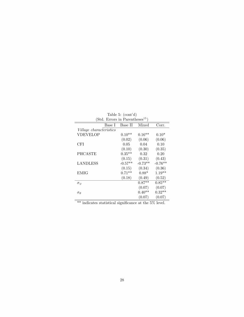
Table 5: (cont’d)(Std. Errors in Parentheses15)

Base I Base II Mixed Corr.Village characteristicsVDEVELOP 0.10** 0.16** 0.10*

(0.02) (0.06) (0.06)CFI 0.05 0.04 0.10

(0.10) (0.30) (0.35)PHCASTE 0.35** 0.32 0.20

(0.15) (0.31) (0.43)LANDLESS -0.57** -0.73** -0.76**

(0.15) (0.34) (0.36)EMIG 0.71** 0.88* 1.19**

(0.18) (0.49) (0.52)σψ 0.87** 0.85**

(0.07) (0.07)σθ 0.40** 0.32**

(0.07) (0.07)** indicates statistical significance at the 5% level.

28

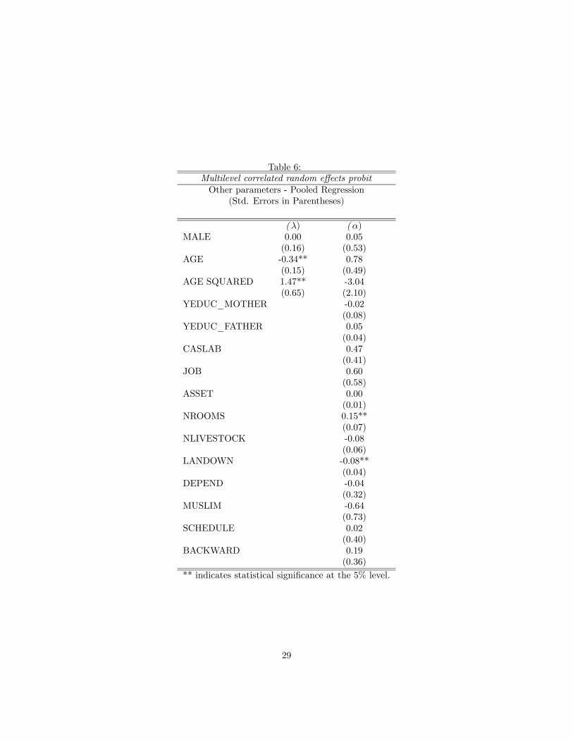
Table 6:Multilevel correlated random effects probitOther parameters - Pooled Regression

(Std. Errors in Parentheses)

(λ) (α)MALE 0.00 0.05

(0.16) (0.53)AGE -0.34** 0.78

(0.15) (0.49)AGE SQUARED 1.47** -3.04

(0.65) (2.10)YEDUC_MOTHER -0.02

(0.08)YEDUC_FATHER 0.05

(0.04)CASLAB 0.47

(0.41)JOB 0.60

(0.58)ASSET 0.00

(0.01)NROOMS 0.15**

(0.07)NLIVESTOCK -0.08

(0.06)LANDOWN -0.08**

(0.04)DEPEND -0.04

(0.32)MUSLIM -0.64

(0.73)SCHEDULE 0.02

(0.40)BACKWARD 0.19

(0.36)** indicates statistical significance at the 5% level.

29

Table 7: Probit Estimates on School Attendance - Uttar Pradesh(Std. Errors in Parentheses)

Base I Base II Mixed Corr.Individual and household characteristicsMALE 0.73** 0.75** 0.93** 0.97**

(0.09) (0.10) (0.10) (0.12)AGE 0.70** 0.71** 0.86** 0.86**

(0.08) (0.09) (0.09) (0.10)AGE SQUARED -3.42** -3.46** -4.17** -4.17**

(0.38) (0.39) (0.41) (0.45)YEDUC_MOTHER 0.12** 0.11** 0.14** 0.14**

(0.03) (0.03) (0.05) (0.05)YEDUC_FATHER 0.10** 0.09** 0.11** 0.10**

(0.01) (0.01) (0.02) (0.02)CASLAB 0.04 0.03 0.06 0.07

(0.10) (0.12) (0.13) (0.14)JOB -0.27** -0.34** -0.41** -0.46**

(0.14) (0.15) (0.19) (0.20)ASSET 0.01* 0.01** 0.01 0.01

(0.00) (0.00) (0.01) (0.01)NROOMS 0.12** 0.12** 0.14** 0.12**

(0.03) (0.03) (0.03) (0.03)NLIVESTOCK -0.02 -0.02 -0.01 -0.01

(0.01) (0.01) (0.02) (0.02)LANDOWN -0.00 -0.00 0.00 0.01

(0.01) (0.01) (0.01) (0.01)DEPEND -0.27** -0.27** -0.29** -0.28**

(0.06) (0.06) (0.08) (0.09)MUSLIM -0.19 -0.23 -0.14 0.05

(0.21) (0.23) (0.38) (0.41)SCHEDULE -0.07 0.01 -0.06 -0.25

(0.11) (0.27) (0.19) (0.21)BACKWARD 0.25** 0.27** 0.30* 0.14

(0.10) (0.12) (0.17) (0.19)Constant -3.55** -3.76** -4.55** -10.78**

(0.46) (0.53) (0.64) (3.33)** indicates statistical significance at the 5% level.

30

Table 7: (cont’d)(Std. Errors in Parentheses)

Base I Base II Mixed Corr.Village characteristicsVDEVELOP 0.17** 0.19** 0.03

(0.04) (0.09) (0.09)CFI -0.34 -0.44 -0.32

(0.27) (0.37) (0.44)PHCASTE 0.33 0.36 -0.09

(0.36) (0.39) (0.59)LANDLESS -0.81** -0.81 -1.47**

(0.38) (0.73) (0.73)EMIG 0.61** 0.75 1.19*

(0.29) (0.56) (0.62)σψ 0.64** 0.63**

(0.10) (0.09)σθ 0.34** 0.18**

(0.09) (0.09)** indicates statistical significance at the 5% level.

31