Determination of frame-dragging using Earth gravity models from CHAMP and GRACE

www.elsevier.com/locate/newast

New Astronomy 11 (2006) 527–550

Determination of frame-dragging using Earth gravity modelsfrom CHAMP and GRACE

I. Ciufolini a,*, E.C. Pavlis b, R. Peron c

a Dipartimento di Ingegneria dell’Innovazione, Universita di Lecce and INFN Sezione di Lecce, Via Monteroni, 73100 Lecce, Italyb Joint Center for Earth Systems Technology (JCET/UMBC), University of Maryland, Baltimore County, 1000 Hilltop Circle, Baltimore, MD 21250, USA

c Dipartimento di Fisica, Universita di Lecce and INFN Sezione di Lecce, Via Arnesano, 73100 Lecce, Italy

Received 28 December 2005; accepted 3 February 2006Available online 23 February 2006

Communicated by G. Setti

Abstract

Using the new generation Earth’s gravity field models EIGEN-2S, GGM01S and EIGEN-GRACE02S generated by the space mis-sions CHAMP and GRACE, we have obtained an accurate measurement of the Lense–Thirring effect with the LAGEOS and LAGEOSII satellites analyzing about 10 years of data with the EIGEN-2S and GGM01S models and about 11 years of data with EIGEN-GRACE02S. This new analysis is in agreement with our previous measurements of the Lense–Thirring effect using the LAGEOS satel-lites and obtained with the JGM-3 and EGM96 Earth’s models. However, the new determinations are more accurate and, especially,more robust than our previous measurements. In the present analysis we are only using the nodal rates of the two satellites, makingno use of the perigee rate, as in our previous analyses. The perigee is affected by a number of non-gravitational perturbations difficultto be modelled and whose impact in the total error budget is not easy to assess. Using the EIGEN-2S model, we obtain a total errorbudget between 18% and 36% of the Lense–Thirring effect due to all the error sources. Specifically, by using EIGEN-2S, we obtain:l = 0.85, with a total error between ±0.18 and ±0.36, with GGM01S we get l = 1.06 with a total error between ±0.19 and ±0.24and with EIGEN-GRACE02S we obtain l = 0.99, with a total error between ±0.05 and ±0.1, i.e., between 5% and 10% of the generalrelativistic predicted value of the Lense–Thirring effect. In addition to the analyses using EIGEN-2S, GGM01S and EIGEN-GRACE02Swithout the use of the perigee, we have also performed an analysis using the older model EGM96 with our previous method of combiningthe nodes of the LAGEOS satellites with the perigee of LAGEOS II. However, this analysis was performed over a period of about 10years, i.e. about 2.5 times longer than any our previous analysis. The result using EGM96 over this longer period of observation agreeswith our previous results over much shorter periods and with the EIGEN-2S, GGM01S and EIGEN-GRACE02S measurements of l. Inaddition to the accurate determination of frame-dragging and in agreement with our previous analyses of the orbits of the LAGEOSsatellites, we have observed, since 1998, an anomalous change in the Earth quadrupole coefficient, J2 which agrees with recent findingsof other authors. This anomalous variation of J2 is accurately observed both on the node of LAGEOS and LAGEOS II and it is inde-pendent of the model used, i.e., it is observed by using the model EGM96 or by using EIGEN-2S, GGM01S or EIGEN-GRACE02S.However, this anomalous variation of the Earth quadrupole coefficient does not affect at all our determination of the Lense–Thirringeffect thanks to the total elimination of the J2-induced errors with our especially devised estimation technique.� 2006 Elsevier B.V. All rights reserved.

PACS: 04.80; 04.80.Ce

Keywords: Gravitation; Relativity; Lense–Thirring; Gravitomagnetism; Laser ranging

1384-1076/$ - see front matter � 2006 Elsevier B.V. All rights reserved.

doi:10.1016/j.newast.2006.02.001

* Corresponding author. Tel.: +39 380 3070772; fax: +39 0765 872212.E-mail addresses: [email protected] (I. Ciufolini), [email protected] (E.C. Pavlis), [email protected] (R. Peron).

mailto:[email protected]



528 I. Ciufolini et al. / New Astronomy 11 (2006) 527–550

1. Introduction

Frame-dragging is one of the fascinating theoretical pre-dictions of general relativity (Misner et al., 1973; Ciufoliniand Wheeler, 1995). The equivalence principle, at the basisof Einstein’s gravitational theory, states that ‘‘locally’’, in asufficiently small spacetime neighbourhood, in a freely fall-ing frame, the observed laws of physics are the laws of spe-cial relativity. However, the axes of these inertial frames,where ‘‘locally’’ the gravitational field is ‘‘unobservable’’,rotate with respect to ‘‘distant stars’’ due to the rotationof a mass or in general due to a current of mass–energy.In general relativity the axes of the local inertial framesare determined by small gyroscopes. Frame-dragging isrelated to the views of Mach and Einstein on the influenceof mass and mass–currents on inertia and inertial frames(Ciufolini and Wheeler, 1995).

In the weak-field and slow-motion limit, general relativ-ity has a remarkable formal analogy with electrodynamics;indeed, in Einstein theory all the phenomena due to a cur-rent of mass can be described in terms of a gravitomagneticfield which is generated by a mass current in the same wayas the magnetic field is generated by an electric current, fur-thermore it obeys to equations formally similar to the onesfor the magnetic field (Ciufolini and Wheeler, 1995). Thegravitomagnetic effect on the orbit of a test particle is thewell-known Lense–Thirring effect (Lense and Thirring,1918; Will, 1985; Ciufolini and Wheeler, 1995).

In astrophysics the gravitomagnetic field of a super-massive black hole has a basic role in some theories of for-mation and alignment of jets in quasars and active galacticnuclei (Thorne et al., 1986). Frame-dragging effects arounda spinning body such as a spinning black hole or a rotatingneutron star or inside a spinning object are intriguing phe-nomena which have been only in part investigated.

Recently, it was pointed out the existence of an, in prin-ciple, observable delay in the propagation time of light, orgravitational waves, inside a spinning shell or around aspinning mass. This ‘‘spin-time-delay’’ might be observedby measuring the delay in the arrival time of differentimages of the same body by gravitational-lensing, assumingthat one would be able to accurately enough model allother larger time delays in the propagation time due toother effects such as geometrical time delay, Shapiro timedelay, etc. (Ciufolini and Ricci, 2002a,b, 2004).

We shall briefly describe the ‘‘spin-time-delay’’ and theother main gravitomagnetic phenomena due to the spinof a body on clocks, light, gyroscopes and test-particles,and the Lense–Thirring effect.

The ‘‘spin-time-delay’’ is equivalent to the impossibilityof everywhere synchronizing clocks in a stationary metric.A photon co-rotating around a spinning body takes lesstime to return to a ‘‘fixed point’’ (with respect to distantstars) than a photon rotating in the opposite direction.For example, around the spinning Earth the differencebetween the travel-time of two pulses of electromagneticradiation counter-propagating in the same circuit would

be �8pJ¯/r, or �10�16 s, where J¯ @ 145 cm2 is the Earthangular momentum (Ciufolini and Wheeler, 1995; Ciufoliniand Ricci, 2002a). Since light rays are used to synchronizeclocks, the different travel-time of co-rotating and coun-ter-rotating photons implies the impossibility of synchroni-zation of clocks all around a closed path around a spinningbody. In several papers the ‘‘frame-dragging clock effect’’around a spinning body has been estimated and space exper-iments have been proposed to test it (Cohen and Mashhoon,1993; Mashhoon et al., 1999; Tartaglia, 2000a,b; Ciufoliniand Ricci, 2002a). When a clock, co-rotating very slowly(using rockets) around a spinning body and at a constantdistance from it, returns to its starting point it finds itselfadvanced relative to a clock kept there ‘‘at rest’’ (withrespect to ‘‘distant stars’’). Similarly a clock counter-rotat-ing arbitrarily slowly, at a constant distance around thespinning body, finds itself retarded relative to the clock atrest at its starting point (Ciufolini and Wheeler, 1995; Ciuf-olini and Ricci, 2002a). For example, when a clock that co-rotates very slowly around the spinning Earth, e.g. at�6000 km altitude, returns to its starting point it finds itselfadvanced relative to a clock kept there ‘‘at rest’’ (withrespect to ‘‘distant stars’’) by �4pJ¯/r � 5 · 10�17 s, whereJ¯/r3 � H¯ and H¯ is the Earth gravitomagnetic field (seebelow). Similarly, a clock that counter-rotates very slowlyaround the spinning Earth finds itself retarded relative toa clock kept there at ‘‘rest’’ by the same amount.

Let us now consider a photon emitted from a distantsource and propagating near a spinning mass. The ‘‘spin-time-delay’’ for the photon, or graviton, travelling forexample on the equatorial plane of a central spinning bodyis then (Ciufolini and Ricci, 2002a):

DT ¼ 4Jb;

where J is the angular momentum of the central body, b theimpact parameter of the photon path and we have consid-ered a simple, ideal configuration where the emitting object(source), deflecting body (lens) and the observer arealigned. In addition to this delay there is the standardShapiro time delay due to the mass of the deflecting bodyand the delay due to the quadrupole moment and highermass moments of the deflecting body, in general we alsohave a geometrical time delay (Schneider et al., 1992) dueto the different geometrical paths followed by the differentrays due to deflection by mass and mass rotation. Depend-ing on the geometry of the system and on the mass distri-bution, this additional term may be very large and maybe the main source of time delay.

In the case of a rotating shell (Thirring, 1918; Weinberg,1972; Ciufolini and Wheeler, 1995) there is also a timedelay in the travel time of photons propagating inside it.Indeed, also inside the shell it is not possible to synchronizeclocks all around a closed path. If we consider a clock co-rotating very slowly with the rotating shell along a circularpath with radius r on its equatorial plane, when it is back toits starting point is advanced with respect to a clock kept

I. Ciufolini et al. / New Astronomy 11 (2006) 527–550 529

there at rest in respect to distant stars. The differencebetween the time read by the co-rotating clock and theclock at rest is equal to dT ¼ �

H h0iffiffiffiffiffiffiffi�g00p dxi ¼ 8M

3Rpxr2; wherex ” (0,0,x) is the angular velocity of the shell.

The spin time delay inside a rotating spherical mass hasbeen calculated in (Ciufolini and Ricci, 2004). The gravito-magnetic vector potential, from the weak field and slowmotion limit of the Einstein’s equations, is given by:Dh0i = 16pqvi, with solution outside a spinning sphere ofradius r (Weinberg, 1972; Ciufolini and Wheeler, 1995):hðxÞ ¼ 2

r3 x� JðrÞ, and inside a hollow spinning sphere ofinternal radius R0 and external radius R: hðxÞ ¼16p

3x�

R RR0

xqr dr, where r . jxj. For a photon on the equa-torial plane of the spinning sphere propagating along thex-axis with impact parameter y = b, the delay in its traveltime, due to the angular momentum of the internal andexternal mass, is:

dT ¼Z ffiffiffiffiffiffiffiffiffi

R2�b2p

�ffiffiffiffiffiffiffiffiffiR2�b2p h0x dx. ð1Þ

In the case of two photons propagating inside the spinningsphere with impact parameters b and b + db, deflected by amass within their paths and finally received by a far obser-ver, the relative spin time delay measured by the observer,due to the angular momentum of the rotating mass, is sim-ply given by the difference of the time delays (1) calculatedfor b and b + db.

Considering some possible astrophysical sources of‘‘spin-time-delay’’, both for photons propagating in thefield of a rotating body or inside a rotating shell, it has beencalculated that there may be an appreciable time delay dueto the angular momentum of these objects (Ciufolini andRicci, 2002a,b, 2004). Thus spin time delay should, in prin-ciple, be taken into account in the modelling of relativetime delays in the images of a far source observed by grav-itational lensing. This effect is due to the propagation ofphotons in opposite directions with respect to the spin ofa body, or shell. The relative time delay in the gravitationallensing images caused by a typical rotating galaxy, or clus-ter of galaxies, was analyzed in Ciufolini and Ricci(2002a,b, 2004). The relative spin time delay was also ana-lyzed when the path of photons is inside a galaxy, a cluster,or a super-cluster of galaxies rotating around the deflectingbody. If time delays of other origin can be accuratelyenough modelled and removed from the observations, thiseffect may be large enough to be measured on Earth. Themeasurement of the spin time delay, due to the angularmomentum of the external massive rotating shell, mightin principle be a further observable for the determinationof the total mass–energy of the external body, i.e. of thedark matter of galaxies, clusters and super-clusters of gal-axies. Indeed, by measuring the spin time delay one maydetermine the total angular momentum of the rotatingbody and thus, by estimating the contribution of the visiblepart, one may determine its rotating dark-matter content.Finally, the possible measurement of the spin time delay

for a pulsar orbiting a spinning body was considered inCiufolini and Ricci (2002a,b, 2004). In conclusion, depend-ing on the geometry of the astrophysical system considered,the relative spin time delay might be an observable effect.

General relativity however predicts the occurrence ofpeculiar phenomena in the vicinity of a spinning body,caused by its rotation, not only on light and clocks but alsoon test-particles. Indeed, the orbital period of a particleorbiting around a spinning body in the same direction asthe rotation of the body, i.e. ‘‘co-rotating’’ with the centralobject, is longer than the orbital period of a particle orbit-ing at the same distance but in the opposite direction, i.e.‘‘counter-rotating’’ with respect to the spin of the centralobject. The difference between the orbital periods of theco-rotating and counter-rotating particles is: Ds = 4pJ/M(Cohen and Mashhoon, 1993; Mashhoon et al., 1999). Fur-thermore, a particle orbiting around a spinning body hasits orbital plane ‘‘dragged’’ around the spinning body inthe same sense as the rotation of the body and small gyro-scopes that determine the axes of a local, freely-falling,inertial frame, where ‘‘locally’’ the gravitational field is‘‘unobservable’’, rotate with respect to ‘‘distant stars’’due to the rotation of the body. Thus, an external currentof mass, such as the spinning Earth, ‘‘drags’’ and changesthe orientation of the gyroscopes. Indeed, a test gyroscopehas a precession with respect to ‘‘an asymptotic inertialframe’’ with angular velocity, in weak field:

_X ¼ � 1

2H ¼ ½�Jþ 3ðJ � xÞx�

jxj3; ð2Þ

where J is the angular momentum of the central object andH its gravitomagnetic field generated by J. This is the‘‘rotational dragging of inertial frames’’, or ‘‘frame-drag-ging’’, as Einstein named it (Pugh, 1959; Schiff, 1960; Ciuf-olini and Wheeler, 1995).

The orbital angular momentum vector of a test particleis itself a kind of gyroscope and is thus dragged by the spinof the central body. Indeed, the node of a test particleorbiting around a central body with angular momentumJ has a secular rate of change. The change of the longitudeof the line of the nodes (intersection between the orbitalplane of the test particle and the equatorial plane of thecentral object), discovered by Lense and Thirring (1918),is in the weak field approximation:

_XLense–Thirring ¼ 2J

½a3ð1� e2Þ3=2�; ð3Þ

where a is the semimajor axis of the test particle, and e itsorbital eccentricity. The Runge–Lenz vector of an orbitingtest particle, for a motion under a central force �1/r2, isalso a kind of gyroscope and is dragged by the spin ofthe central body. Indeed, the pericenter of an orbiting testparticle around a central body with angular momentum Jhas a secular rate of change. The change of the longitudeof the pericenter ~x ¼ Xþ x (defining the Runge–Lenz vec-tor), where x is the argument of the pericenter that is theangle from the central body equatorial plane to the pericen-


ter, discovered by Lense and Thirring (Lense and Thirring,1918), is in weak field:

_~xLense–Thirring ¼ 2JðJ� 3 cos I lÞ½a3ð1� e2Þ3=2�

;

where l is the orbital angular momentum unit vector of thetest particle and I its orbital inclination (angle between theorbital plane and the equatorial plane of the central object).

In Einstein’s general theory of relativity all these phe-nomena, on test particles, gyroscopes, photons and clocks,are the result of the rotation of a mass and, in general, ofmass–energy currents (Ciufolini and Wheeler, 1995).

In 1995–2001 the Lense–Thirring effect was observedusing the LAGEOS and LAGEOS II satellites (Ciufolini,1986, 1989, 1996; Ciufolini et al., 1996, 1997, 1998).

The basic components used in our older approach todetect the Lense–Thirring effect were: (1) the very accu-rately tracked orbits of the laser-ranged satellites LAGEOSand LAGEOS II, (2) the accurate Earth gravity modelsJGM-3 and EGM96 and (3) three observables: the twonodes of LAGEOS and LAGEOS II and the perigee ofLAGEOS II, in order to cancel the error due to the uncer-tainties in the Earth quadrupole moment, J2 and in the nextlargest even zonal harmonic, J4, and thus to measure theLense–Thirring effect; i.e., in order to use three observablesfor the three unknowns: Lense–Thirring effect, dJ2 and dJ4.

Table 1Models used in the orbital analysis

Geopotential (static part) EIGEN-2S, GGM01S,EIGEN-GRACE02S

Geopotential (tides) Ray GOT99.2Lunisolar and planetary perturbations JPL ephemerides DE-403General relativistic corrections PPN except L–TLense–Thirring effect Set to zero

Direct solar radiation pressure Cannonball modelAlbedo radiation pressure Knocke–Rubincam modelYarkovsky–Rubincam effect GEODYN modelSpin axis evolution of LAGEOS

satellitesFarinella–Vokhroulicky–Barliermodel

Station positions (ITRF) ITRF2000Ocean loading Scherneck model with

GOT99.2 tidesPolar motion EstimatedEarth rotation VLBI + GPS

2. Method of the present analysis

The accurate measurements of the Lense–Thirring effectdescribed in this paper have been obtained by using thelaser-ranging data of the satellites LAGEOS (LAser GEO-dynamics Satellite) and LAGEOS II (Cohen and Dunn,1985; Bender and Goad, 1979) and the recently releasedEarth gravitational field models EIGEN-2S, GGM01Sand EIGEN-GRACE02S (Perosanz et al., 2003; Reigberet al., 2002, 2003, 2005; Rummel, 2003; Tapley, 2002; Wat-kins et al., 2002) (see Section 3). In addition we also used theolder model EGM96 with our previous method of includingthe perigee rate of LAGEOS II; however the present periodof analysis covers a period of about 10 years, i.e. about 2.5times longer than in any our previous analysis.

The LAGEOS satellites are heavy brass and aluminumsatellites, of about 406 kg weight, completely passive andcovered with retro-reflectors, orbiting at an altitude of about6000 km above the surface of Earth. LAGEOS, launched in1976 by NASA, and LAGEOS II, launched by NASA andASI (the Italian Space Agency) in 1992, have an essentiallyidentical structure but they have different orbits. The semi-major axis of LAGEOS is a @ 12,270 km, the periodP @ 3.758 h, the eccentricity e @ 0.004 and the inclinationI @ 109.9�. The semimajor axis of LAGEOS II isaII @ 12,163 km, the eccentricity eII @ 0.014 and the inclina-tion III @ 52.65�. We have analyzed the laser-ranging datausing the principles described in IERS (1997) and adoptedthe IERS conventions in our modelling, except that, in our

recent analyses, we used the Earth static gravity modelsEIGEN-2S, GGM01S and EIGEN-GRACE02S. Our anal-ysis was performed using 15-day arcs. For each 15-day arc,initial state vector (position and velocity), coefficient ofreflectivity (CR) and polar motion were adjusted. Solar radi-ation pressure, Earth albedo, and anisotropic thermal effectswere modelled according to (Rubincam, 1988, 1990; Rubin-cam and Mallama, 1995; Martin and Rubincam, 1996). Inmodelling the thermal effects, the orientation of the satellitespin axis was obtained from Andres et al. (2004). We haveapplied a _J 4 ¼ �1:41� 10�11 correction to the modelsEIGEN-2S and GGM01S, which was already included inEIGEN-GRACE02S (Reigber et al., 2005; Ciufolini andPavlis, 2005); see Appendix A. Lunar, solar, and planetaryperturbations were also included in the equations of motion,formulated according to Einstein’s general theory of relativ-ity with the exception of the Lense–Thirring effect, whichwas purposely set to zero. Polar motion was adjusted andEarth’s rotation was modelled from the very long baselineinterferometry-based series SPACE (Gross, 1996) whichare extended annually. We analyzed the laser-ranging dataand the orbits of the LAGEOS satellites using the orbitalanalysis and data reduction software GEODYN II (Pavliset al., 1998). The models used are listed in Table 1.

In Section 1 we have seen how the node and the perigeeof a test-particle are dragged by the angular momentum of acentral body. From the Lense–Thirring formula (3), we getfor the nodes of the satellites LAGEOS and LAGEOS II:_XLense–Thirring

I ffi 31 mas=yr and _XLense–ThirringII ffi 31:5 mas=yr,

where mas is a millisecond of arc. The argument of pericen-ter (perigee in our analysis), x, of the LAGEOS satelliteshas also a Lense–Thirring drag (Ciufolini et al., 1998).However, whereas in our previous determination of theLense–Thirring effect (Ciufolini et al., 1998) we used boththe nodes of LAGEOS and LAGEOS II and the perigeeof LAGEOS II, in the present analyses we only use thenodes of LAGEOS and LAGEOS II. Indeed, the perigeeof an Earth satellite such as LAGEOS II is affected by anumber of perturbations whose impact in the final error


budget is not easy to be assessed and this was one of the twomain points of concern of Ries et al. (2003a). The otherpoint of concern was some favorable correlation of theerrors of the Earth’s spherical harmonics for the EGM96model that might lead to some underestimated error bud-get. However, these points of concern are absent in the pres-ent analyses, see Sections 3 and 4. Indeed, using theprevious models JGM-3 and EGM96, we were forced touse three observables and thus we also needed to use theperigee of LAGEOS II. However, with the recently releasedsolutions EIGEN-2S, GGM01S and EIGEN-GRACE02S(Perosanz et al., 2003; Reigber et al., 2002, 2003, 2005;Rummel, 2003; Tapley, 2002; Watkins et al., 2002), thanksto the more accurate determination of the Earth’s gravityfield, it is just enough to eliminate the uncertainty in theEarth’s quadrupole moment and thus to just use twoobservables, i.e. the two nodes of the LAGEOS satellites.However, we have also determined the Lense–Thirringeffect with EGM96 and the use of the perigee of LAGEOSII, over about 10 years of data. There was a remarkableagreement using these different techniques and the differentEarth gravity models.

To precisely quantify and measure the gravitomagneticeffects we have introduced the parameter l that is by defi-nition 1 in general relativity (Ciufolini and Wheeler, 1995)and zero in Newtonian theory.

The main error in this measurement is due to the uncer-tainties in the Earth’s even zonal harmonics and their timevariations. The un-modelled orbital effects due to the har-monics of lower degree are of order of magnitude compara-ble to the Lense–Thirring effect (see Section 4). However, byanalyzing the EIGEN-2S, GGM01S and EIGEN-GRACE02S models and their uncertainties in the evenzonal harmonics, and by calculating the secular effects ofthese uncertainties on the orbital elements of LAGEOSand LAGEOS II, we find that the main source of error inthe determination of the Lense–Thirring effect is just dueto the first even zonal harmonic, J2 (see Section 4).

We can however use the two observable quantities _XI

and _XII to determine l (Ciufolini, 1986, 1989, 1996,2002), thereby avoiding the largest source of error arisingfrom the uncertainty in J2. We do this by solving the systemof the two equations for d _XI and d _XII in the two unknownsl and J2, obtaining for l:

d _XExpLAGEOS I þ cd _XExp

LAGEOS II ¼ lð31þ c31:5Þ mas=yr

þ other errors

ffi lð48:2 mas=yrÞ; ð4Þ

where c = 0.545 (the key idea of using the nodes of two laser-

ranged satellites of LAGEOS type to measure the Lense–Thir-

ring effect was first published in Ciufolini (1984, 1986) andlater studied in Tapley et al. (1989–2004). The use of sucha combination of the nodes only of a number of laser-rangedsatellites was first explained in Ciufolini (1989, p. 3102),see also Ciufolini and Wheeler (1995, p. 336), where it is writ-ten ‘‘. . . A solution would be to orbit several high-altitude,

laser-ranged satellites, similar to LAGEOS, to measure J2,J4, J6, etc., and one satellite to measure _XLense–Thirring . . .’’.The use of the nodes of LAGEOS and LAGEOS II, togetherwith the explicit expression of the LAGEOS nodal equa-tions, was first proposed in Ciufolini (1996); the explicitexpression of this combination, that is however a trivial stepon the basis of the explicit equations given in Ciufolini(1996), was presented by one of us during the 2002 I-SI-GRAV school and published in its proceedings (Ciufolini,2002). For a study of the determination of the Lense–Thir-ring effect using laser-ranged satellites see also (Peterson,1997). The use of the GRACE-derived gravitational models,when available, to measure the Lense–Thirring effect withaccuracy of a few percent was, since many years, a wellknown possibility to all the researchers in this field andwas presented by one of us during the SIGRAV 2000 confer-ence (Pavlis, 2002) and published in its proceedings, and waspublished by Ries et al. in the proceedings of the 1998William Fairbank conference and of the 2003 13th Int. LaserRanging Workshop (Ries et al., 2003a,b), where Ries et al.concluded that, in the measurement of the Lense–Thirringeffect using the GRACE gravity models and the LAGEOSand LAGEOS II satellites: ‘‘a more current error assessmentis probably at the few percent level. . .’’).

Eq. (4) for l does not depend on J2 nor on its uncer-tainty; thus, the value of l that we obtain is unaffectedby the largest error, due to dJ2, and it is sensitive only tothe smaller uncertainties due to dJ2n, with 2n P 4.

Similarly, regarding tidal, secular and seasonal changesin the geopotential coefficients, the main effects on the nodesof LAGEOS and LAGEOS II, caused by tidal and othertime variations in Earth’s gravitational field (Ciufolini,1989; Ciufolini et al., 1998), are due to changes in the quad-rupole coefficient J2, e.g., by the 18.6 year Lunar tide withthe period of the Moon node and by the post-glacialrebound, and due to anomalous variations of J2 (see Section4). However, the tidal errors in J2 and the errors resultingfrom other un-modelled, medium and long period, timevariations in J2, including its secular and seasonal varia-tions, are cancelled by our combination of the node residu-als (4). In particular, most of the errors resulting from the18.6 and 9.3 years tides, associated with the lunar node,are cancelled in our measurement. The various error sourcesthat can affect the measurement of the Lense–Thirring effectusing the nodes of the LAGEOS satellites have been exten-sively treated in a large number of papers by several authors,see, e.g., Ciufolini (1986, 1989, 1996), Ciufolini et al. (1998,1997), Rubincam (1988, 1990), Rubincam and Mallama(1995), Martin and Rubincam (1996), Andres et al. (2004),Lucchesi (2001, 2002), Iorio (2001), Pavlis and Iorio(2002); the main error sources are treated here in Section 4.

3. The gravity field models EIGEN-2S, GGM01S and

EIGEN-GRACE02S

For many decades geodesy facilitated the testing of somebasic laws of physics. An area that space geodesy contrib-


utes the most, is the precise determination of the terrestrialgravity field and its temporal variations. This provides theprecise, stable and free-of-gravitational-noise environmentwhere very delicate experiments in gravitational physicsare conducted. Until the mid-90s, the geodesists attentionwas centered on the static field, mainly because of the needto compute precise orbits for satellites carrying variousinstruments (Lemoine et al., 1997, 1998). Since the emer-gence of climate change as one of the most importantresearch topics at the international level (NRC, 1997), thetemporal variations of the gravity field have become a primetopic and the focus of several space missions with clearlyinternational nature. These proposed missions generatedgreat expectations within the fundamental physics commu-nity (Pavlis, 1993). Some of the proposed missions arealready in orbit now: CHAMP, launched July 15, 2000;GRACE, launched March 17, 2002 and some are still underdevelopment: GOCE, planned for a late-2006 launch.

The first mission, CHAMP, has delivered a number ofglobal models of the static gravitational field: EIGEN-1S,EIGEN-2S, EIGEN-3p (Reigber et al., 2002, 2003). Theinnovative aspect of this mission is its precise tracking fromthe Global Positioning System (GPS) constellation of satel-lites and the simultaneous measurement of non-gravita-tional forces from an on-board precise accelerometer(Perosanz et al., 2003). This is the first time that such anaccelerometer is used for an extended mission. Due to thehigh altitude of the GPS spacecrafts (12 h orbits) and thelow altitude of CHAMP (400 km), the configuration iscalled high–low (H–L) satellite-to-satellite tracking (SST).The benefit of this configuration is that the entirety ofthe unaccounted perturbations in the observed range-ratebetween the two spacecraft can be now attributed toun-modelled gravitation sensed by the low orbiter (non-gravitational forces are accounted for using the observedaccelerometer measurements). The model enhancementfrom CHAMP is primarily the accuracy improvement ofthe very low degree terms (long wavelengths) up to about40�, to roughly two orders of magnitude better than whatwas available from EGM96.

The second mission, GRACE, is a pair of CHAMP-likespacecraft flying in tandem formation (nominally 250 kmapart), enhanced with higher quality accelerometers and aone-way radio frequency range-difference measuring systemon both of them. This configuration of satellite-to-satellitetracking between two low orbiters is called low–low (L–LSST). The L–L configuration is characterized from its abil-ity to resolve features proportional to the distance betweenthe two spacecraft. GRACE therefore, since it also carriesGPS receivers on both spacecraft, contributes to the obser-vation of the long, as well as the medium wavelengths (up to120) of the gravitational spectrum. Moreover, the mission ispolar (i = 89.5�) and it samples the field well enough to pro-duce monthly snapshots. With a projected lifetime of fiveyears, it is hoped that we will acquire enough such monthlysnapshots to be able to determine the temporal variations inthe long wavelengths down to at least seasonal frequencies.

This achievement alone is a unique contribution comparedto today’s status quo. To date, only the secular variations ofthe first few zonal terms up to 6� have been studied on thebasis of perturbation analysis from ground-based trackingdata. Annual and semi-annual signals have been determinedonly for J2 and J3, and these are not as definitive and robustresults as we would like to have. The first, preliminary mod-els based on GRACE data alone (Tapley, 2002; Watkinset al., 2002; Reigber et al., 2003, 2005) show significantimprovements in the accuracy of the static part of the fieldand especially so for the long wavelength terms, reachingalmost two orders of magnitude improvements comparedto EGM96 (Tapley, 2002). Unfortunately, the covariancematrix of these models is not yet available.

The third mission, GOCE, is really the true geopotentialmapping mission that geodesists always hoped for sincethe early 70s (Rummel, 2003). Instead of relying on pertur-bations from which to infer the gravitational signal (as inH–L and L–L), GOCE will carry a gradiometer, a device thatwill measure directly the gravitational tensor components inspace. Along with precise knowledge of the time and loca-tion of these measurements (GOCE will also be tracked withGPS), we can then construct a gravitational model solving ageodetic boundary problem by means of one of the standardgeodetic techniques. Although this task is not as simple as itsounds, gradiometry is definitely the cleanest and most directmeasurement of gravitation that we could possibly make inspace. With a two six-month observing periods scenario,GOCE promises to deliver a model that will extend our pre-cise knowledge to much higher resolution, somewhere in theneighborhood of maximum degree 220–250. It is expectedthat by that time, the release of additional observations onland and over the oceans, from national data bases and ter-restrial campaigns (airborne and ship-borne), will allow thedevelopment of global models to maximum degree >200.While these models will not have the same uniform qualityfor the very high degree portions (above 250) on a globalscale, their overall improvement will remove all of the ambi-guities associated with the static long and medium wave-lengths. The temporal signals will also be preciselyobserved thanks to GRACE. This multitude of gravitationalmodelling missions is the reason for calling the present dec-ade the International Decade for Geopotential Research.

The present re-analysis of the SLR data set selected theCHAMP- and GRACE-based models (Reigber et al.,2002, 2003, 2005) as the underlying gravitational models,primarily because of their pedigree, i.e., the independencefrom any tracking data other than that from CHAMP orGRACE, and the high quality low degree performance ofthe models. It is worth describing briefly these models, inorder to appreciate their contribution and significance tothe success of this experiment. The EIGEN2S model isbased solely on CHAMP data for a total of 180 days(Aug.–Dec. 2000 and Sept.–Dec. 2001). The data pool com-prised GPS SST at 30 s intervals (phase and pseudo-range),three-axes accelerometer measurements from the STARaccelerometer (Perosanz et al., 2003) at 10 s intervals, and


the orientation of CHAMP from star-camera observationsat 10 s intervals. Additionally, data for thruster firings wereconsidered in the analysis, describing the epoch and dura-tion of operation for the three pairs of on-board thrusters.The model comprises a complete set of spherical harmonicrepresentation to degree and order 120, with additionalzonal and resonant terms to 140�. The ocean tidal potentialfor the diurnal and semi-diurnal periods was also estimatedsimultaneously in the solution. The only external informa-tion was the addition of conditioning information for thestabilization of the solution (derived from a single satellite).For this purpose, the empirical geopotential power spec-trum after Kaula was used for the terms above 30�. Thishas no impact in our experiment, since the orbit of LAG-EOS-like spacecraft is practically insensitive to terms abovedegree and order 20, even for arcs as long as one month. Aswe already pointed out earlier, the new model brings inde-pendent information in this experiment. The gravitationalpotential, and especially the low degree terms, are no longerderived from the analysis of the same (or similar) data thatare used to perform this experiment. It is therefore clear thatthere can be no incestuous relationship between the resultsof this experiment and the model used for the orbital com-putations. Furthermore, we must remark on the quality ofthe accuracy estimate of the new model. The EIGEN-2Scoefficients and, in particular, the zonal terms are not thatdifferent from those of EGM96. There is however a veryimportant difference in terms of their accuracy estimates.Although the publicly available covariance matrix ofEIGEN-2S has not been properly calibrated and the usersare warned of that, a calibration process will not affect thestructure of the covariance matrix, since it is a scaling pro-cess. The structure, on the other hand, describes the corre-lation between the estimated constituents and here is theclear advantage of EIGEN-2S and the follow-on modelsderived from GRACE, over EGM96. While in the case ofthe latter the zonal terms always exhibited high correla-tions, well over 90%, in the case of EIGEN-2S one is hardlypressed to find anything above 30%! Based on the examina-tion of the new model with respect to independent data sets(Pavlis, 2003) it is concluded that the overall description ofthe field is not so different from that of EGM96 and this isespecially true for the low degree terms. The major differ-ence of the new model however and the one with a greatimpact in our experiment is the predominantly diagonalstructure of its correlation matrix. This nature of the errorspectrum of the model results in far more robust estimatesfor the uncertainty associated with our estimate of theLense–Thirring effect from our experiment, reduces theleakage of error between the considered and the neglectedzonal terms, and avoids the danger of fortuitous error can-cellation resulting in overly optimistic results.

The GGM01S model is the first GRACE-only staticgravity model from the UTX/CSR group (Tapley et al.,2003), based on a significant number of GRACE observa-tions (111 days). The model is complete to degree and order120, however, it is recommended that for precise work one

should limit it to degree and order 95. The associated errormodel predicts a geoid accuracy of 2 cm at 70�. This model isnow superseded by the release of GGM02S (November2004), a model based on 363 days of GRACE data, completeto degree and order 160, although it is again recommendedto limit its use to the 120 · 120 part. The release of the sec-ond GGM02S model allowed for a validation of the errorestimates quoted for the first GGM01S model. This givesus some confidence that our error propagation in estimatingour uncertainty in the Lense–Thirring estimate is also cor-rect. The release of the second GGM02S model indicatesthat the unprecedented gravity modeling improvement thatwe saw in the release of the first GGM01S model, in compar-ison to the previously used EGM96 model, was the definitiveimprovement from GRACE. Subsequent releases of modelsbased on increasingly more extensive GRACE data sets willonly marginally improve upon the quality of the previousmodels. Nevertheless, the addition of more data, spreadover increasingly longer time intervals, will definitely drivethe errors associated with all harmonics describing the fieldto even lower levels, thereby increasing their accuracy andconsequently the accuracy of other results that are derivedon that basis (e.g. precise orbits, geophysical parametersand of course, the Lense–Thirring parameter).

The EIGEN-GRACE02S model is the second GRACE-only static gravity model from the GFZ group (Reigberet al., 2005), derived from 110 days of GRACE only satel-lite-to-satellite observations. The model is complete todegree and order 150 and claims an accuracy of 1 mm ingeoid heights at half-wavelength of 800 km, reaching 1 cmat 75�. The errors associated with this model have been cal-ibrated using surface gravimetry, oceanographic data andprecise satellite tracking data. The improvement over previ-ous solutions (e.g. GGM01S and EIGEN-GRACE01S) isattributed to the better data reduction strategy in the caseof EIGEN-GRACE02S. The EIGEN-GRACE02S modelis discussed and used in Ciufolini and Pavlis (2004, 2005).

4. Results: measurement of the Lense–Thirring effect and its

uncertainty

4.1. Error budget

The orbital perturbations of a satellite orbiting around amassive body may be divided in secular and periodic.Among the secular perturbations of the node of the LAG-EOS satellites there are: the shift of the nodal line due tothe even zonal harmonics of the Earth’s gravitational field(Kaula, 1966), the de Sitter effect and frame-dragging.The de Sitter effect has been measured with an accuracyof about 7 · 10�3, its effect is only 19.2 mas on the LAG-EOS node and thus its uncertainty is negligible in theLense–Thirring measurement, however the uncertainty inthe even zonal harmonics is a crucial factor for the determi-nation of frame-dragging since an error in one of the lowereven zonal harmonics may be large enough to be indistin-guishable from the Lense–Thirring nodal drag. This critical

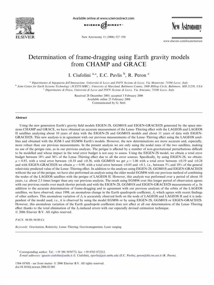
Fig. 1. Fit of the residuals of the nodes of LAGEOS and LAGEOS II,using our combination (4) and the model EIGEN-2S, with a seculartrend only. The slope is l . 0.82, the RMS of the post-fit residuals is15.5 mas.

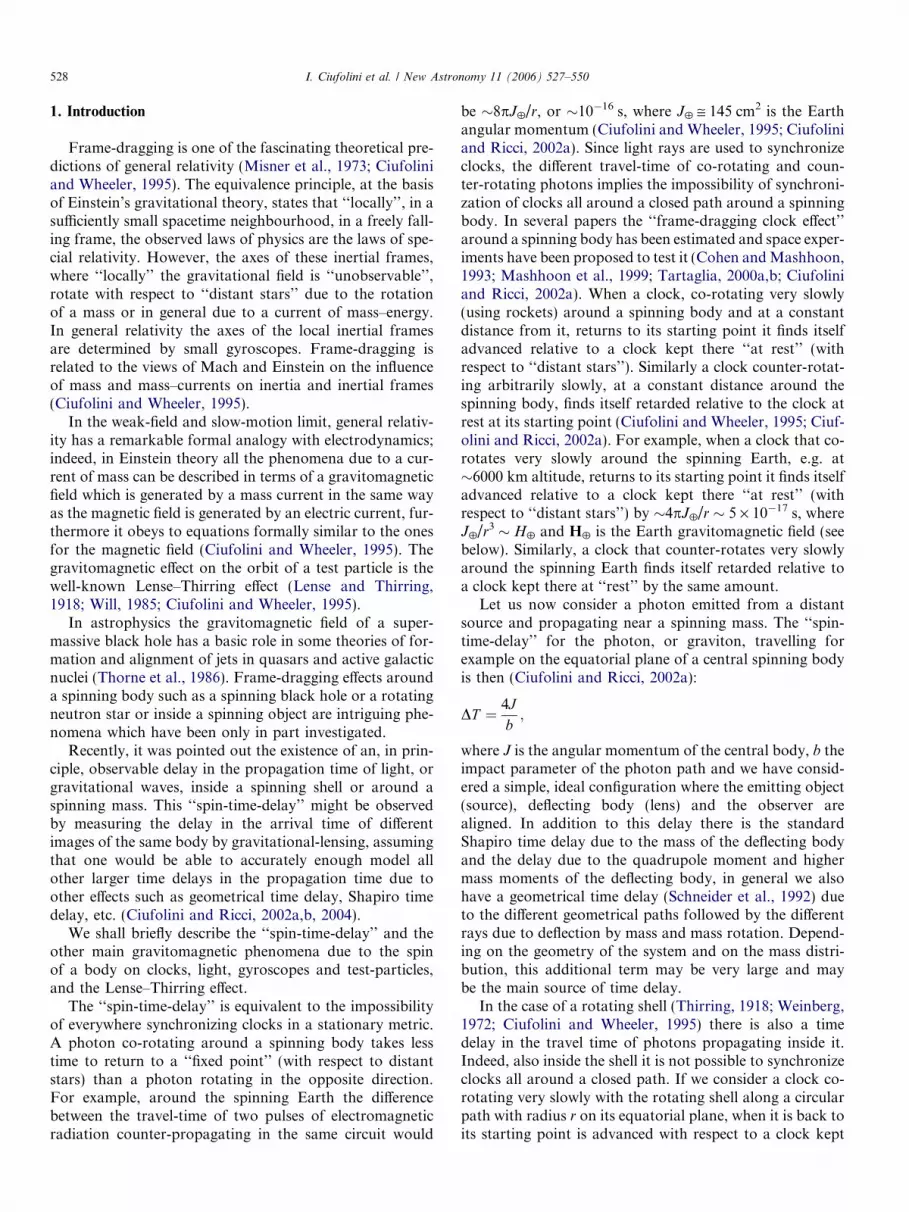
Fig. 2. Fit of the residuals of the nodes of LAGEOS and LAGEOS II,using our combination (4) and the model EIGEN-2S, with a secular trendplus two periodic terms. The slope is l . 0.82, the RMS of the post-fitresiduals is 12 mas.


type of error is treated below. However, the periodic pertur-bations of the node of the LAGEOS satellites may also be acrucial factor in the determination of frame-dragging, par-ticularly crucial is the uncertainty in the perturbations withlong period compared to the period of observation. Theperiodic effects with period much shorter than the observa-tional period are averaged out. In the present determinationof the Lense–Thirring effect, we have three basic factors thatmake negligible the error due to periodic effects in the mea-surement of frame-dragging and also make this error easyto be assessed in the final error budget. These basic factorsare: (i) the period of the present analyses is about 10 years(11 years for EIGEN-GRACE02S) and thus all the periodicperturbations of the nodes are basically averaged out apartfrom the 18.6 years tide associated with the lunar node,however, as explained below, the main effect of this tide isa change of the J2 coefficient that is cancelled out usingour combination of observables (4); (ii) since the originalproposal of the LAGEOS III experiment (Ciufolini,1986), numerous researchers (Ciufolini, 1986, 1989, 1996;Ciufolini et al., 1998, 1997; Rubincam, 1988, 1990; Rubin-cam and Mallama, 1995; Martin and Rubincam, 1996;Andres et al., 2004; Lucchesi, 2001, 2002; Iorio, 2001; Pavlisand Iorio, 2002) have treated, in many papers and reports,the perturbations affecting the LAGEOS node in order todetermine the Lense–Thirring effect and have concludedthat the only critical perturbations on the nodes of theLAGEOS satellites are those due to the Earth’s even zonalharmonics. However, as shown below, due to the highaccuracy of the recent novel Earth’s gravity field modelsEIGEN-2S, GGM01S and EIGEN-GRACE02S, the evenzonal harmonic uncertainties contribute with an errorbetween 17.8% (calculated using the EIGEN-2S covariancematrix) and 36% (summing the absolute values of theerrors) using the uncertainties of the EIGEN-2S model,with an error between 18.8% and 23.5% using GGM01S,and between 3% and 4% using EIGEN-GRACE02S,respectively calculated as root-sum-square of the even zonalharmonics uncertainties and by simply summing the abso-lute values of the even zonal errors of GGM01S andEIGEN-GRACE02S on our combined residuals; (iii) inregards to the periodic perturbations, in addition to adetailed treatment of the various perturbations affectingthe LAGEOS node and their uncertainties given below, asimple but very meaningful test shows that the periodic per-turbations cannot introduce an error larger than about 3%in our determination of the Lense–Thirring effect (�2% inthe longer period analysis with EIGENGRACE02S). Sincethe period of the gravitational and non-gravitational orbitalperturbations (but not their amplitude) is very well deter-mined, we have also fitted, together with a secular trend, anumber of periodic effects. We have done a number of dif-ferent fits, each with different periodic perturbations, wehave then compared the result in the case of the fit with asecular trend only with the various results when, togetherwith a secular trend, we have included a different numberof the main periodic perturbations. The result is that the

maximum deviation of the secular trend from the bench-mark case of its fit with no periodic perturbations doesnot exceed � 3% of Earth’s frame-dragging (�2% in thelonger period analysis with EIGENGRACE02S), as it isdisplayed in Figs. 1–8 and 11–14 and discussed in the corre-sponding captions. Of course the RMS of the fit is muchsmaller when we allow in the fit for a substantial numberof periodic perturbations. Therefore, the two points of con-cerns of Ries et al. (2003a), regarding really not the methodor the resulting value of the Lense–Thirring effect that wehad obtained in our previous analyses (Ciufolini et al.,1997, 1998; Ciufolini, 1994) but rather our previous errorbudgets (claimed by Ries et al. to be optimistic by a factor

Fig. 5. Fit of the residuals of the nodes of LAGEOS and LAGEOS II,using our combination (4) and the model GGM01S, with a secular trendonly. The slope is l . 1.06, the RMS of the post-fit residuals is 15.4 mas.

Fig. 3. Fit of the residuals of the nodes of LAGEOS and LAGEOS II,using our combination (4) and the model EIGEN-2S, with a secular trendplus six periodic terms. The slope is l . 0.85, the RMS of the post-fitresiduals is 6 mas.

Fig. 4. Fit of the residuals of the nodes of LAGEOS and LAGEOS II,using our combination (4) and the model EIGEN-2S, with a secular trendplus ten periodic terms. The slope is l . 0.85, the RMS of the post-fitresiduals is 5.5 mas.

Fig. 6. Fit of the residuals of the nodes of LAGEOS and LAGEOS II,using our combination (4) and the model GGM01S, with a secular trendplus two periodic terms. The slope is l . 1.05, the RMS of the post-fitresiduals is 11.4 mas.


2 or 3), are no longer of concern in the present analyses, asexplained below and in Section 3. Indeed, (i) the concernregarding the perturbations of the perigee of LAGEOS IIis clearly absent in the present analyses since here we onlyuse the nodes of the LAGEOS satellites and we do not usethe perigee, (ii) the concern regarding the high correlationof some of the even zonal harmonics of the EGM96 modelis also absent in the present analyses since the new Earthmodels EIGEN-2S, GGM01S and EIGEN-GRACE02Sused here have low correlation between the even zonal har-monics (see below and related discussion in Section 3). Fur-thermore, to evaluate the even zonal harmonic inducederror in the case of the GGM01S and EIGEN-GRACE02Smodels, we did not use any covariance matrix, instead we

simply added the absolute values of the errors on our com-bined residuals due to the even zonals uncertainties.

In conclusion, in the analysis with EIGEN-2S, we have atotal error budget of about 36% of the Lense–Thirring effect,calculated by summing up the absolute values of theEIGEN-2S even zonal harmonic errors. However, in theanalysis with GGM01S and EIGEN-GRACE02S the totalerror budget drops to 24% for GGM01S and to about 10%for EIGEN-GRACE02S (see more details below). The mainperturbations in our determination of the Lense–Thirringeffect are described and examined in detail in Appendix A.

In the present analysis we have used EIGEN-2S,GGM01S and EIGEN-GRACE02S, however, the modelsEIGEN-2S and GGM01S are preliminary in the sense that

Fig. 9. Residuals of the node of LAGEOS using EIGEN-GRACE02S.

Fig. 8. Fit of the residuals of the nodes of LAGEOS and LAGEOS II,using our combination (4) and the model GGM01S, with a secular trendplus ten periodic terms. The slope is l . 1.06, the RMS of the post-fitresiduals is 6.7 mas.

Fig. 7. Fit of the residuals of the nodes of LAGEOS and LAGEOS II,using our combination (4) and the model GGM01S, with a secular trendplus six periodic terms. The slope is l . 1.07, the RMS of the post-fitresiduals is 7 mas.


they have been obtained from relatively short periods ofobservations of CHAMP and GRACE. Thus, the valuesof the spherical harmonic coefficients describing Earth’sgravity field may appreciably change with longer periodsof observations. In particular, the uncertainties in the zonalharmonics in the case of the GGM01S model includesystematic errors only tentatively and in the case ofEIGEN-2S we only have formal error estimates. However,our analysis is not sensitive to changes in the Earth’s quad-rupole moment and it is only affected by changes in thehigher zonal harmonics. Therefore, in the future, moreaccurate determinations of the even zonal coefficients andof their uncertainties might lead to slightly different values

of l and consequently to a slightly different total error bud-get. As a matter of fact using EIGEN-GRACE02S, whoseuncertainties in Earth’s even zonal harmonics include sys-tematic errors to certain extent, the contribution of theeven zonal errors to the total error budget is 3–4% only.Thus, it is crucial to note that when a more accurate modelusing GRACE, CHAMP or GOCE will be available, it willbe straightforward to, a posteriori, very accurately re-assess the total error of our present analyses. This will bedone by simply taking the differences between the valuesof the even zonals of the presently used models (EIGEN-2S, GGM01S and EIGEN-GRACE02S) with the corre-sponding values of the future, more accurate, models andby considering the uncertainties of these future models.Thus, one will be able to easily re-estimate the total errorin the present measurement of l.

4.2. Results

In this section, we present the latest results in the mea-surement of the Lense–Thirring effect on the basis of thethree different Earth gravitational models, through theanalysis of the nodal rates of the LAGEOS and LAGEOSII satellites. The results displayed in Figs. 1–8 show ourmeasurement of the Lense–Thirring effect, obtained respec-tively using the models EIGEN-2S and GGM01S, and thenodal rates of the LAGEOS and LAGEOS II satellites overa period of about 10 years. In Fig. 9 we plot the integratedresiduals of the node of LAGEOS using the Earth gravitymodel EIGEN-GRACE02S over a period of about 11years. Fig. 10 shows the integrated node residuals of LAG-EOS II using EIGEN-GRACE02S over a period of about11 years. Figs. 11–14 show our measurement of the Lense–Thirring effect obtained using the model EIGEN-GRACE02S and the nodal rates of the LAGEOS andLAGEOS II satellites over a period of about 11 years.

Fig. 1 displays the combination of the nodes, accordingto formula (4), using the EIGEN-2S model. Figs. 2–4 show

Fig. 11. Fit of the residuals of the nodes of LAGEOS and LAGEOS II,using our combination (4) and the model EIGEN-GRACE02S, with asecular trend only. The slope is l . 0.984, the RMS of the post-fitresiduals is 15.4 mas.

Fig. 12. Fit of the residuals of the nodes of LAGEOS and LAGEOS II,using our combination (4) and the model EIGEN-GRACE02S, with asecular trend plus two periodic terms. The slope is l . 0.97, the RMS ofthe post-fit residuals is 11.3 mas.

Fig. 13. Fit of the residuals of the nodes of LAGEOS and LAGEOS II,using our combination (4) and the model EIGEN-GRACE02S, with asecular trend plus six periodic terms. The slope is l . 0.994, the RMS ofthe post-fit residuals is about 6 mas.

Fig. 10. Residuals of the node of LAGEOS II using EIGEN-GRACE02S.


our measurement of the Lense–Thirring effect usingEIGEN-2S by fitting the orbital residuals with a seculartrend together with 2, 6 and 10 main periodic effects.

Fig. 5 displays the combination of the nodes, accordingto formula (4), using GGM01S. Figs. 6–8 show our mea-surement of the Lense–Thirring effect using GGM01S byfitting the orbital residuals with a secular trend togetherwith 2, 6 and 10 periodic effects.

In Fig. 9 we plot the integrated residuals of the node ofLAGEOS from January 1993 to October 2003 using theEarth gravity model EIGEN-GRACE02S. Fig. 10 showsthe integrated node residuals of LAGEOS II usingEIGEN-GRACE02S. Fig. 11 displays the combination ofthe nodes, according to formula (4), using EIGEN-GRACE02S. Figs. 12–14 show our measurement of theLense–Thirring effect using EIGEN-GRACE02S by fitting

the orbital residuals with a secular trend together with 2, 6and 10 periodic effects. Figs. 13 and 14 represent our bestmeasurement of the Lense–Thirring effect: their slope isabout 0.99l.

The slopes of Figs. 2, 3, 4 and 6, 7, 8 are respectively:0.82l, 0.85l, 0.85l, 1.05l, 1.07l and 1.06l. The slopes ofFigs. 12–14 are respectively: 0.97l, 0.99l, and 0.99l.

In conclusion, by fitting our combined residuals with asecular trend only, using EIGEN-2S we found: l = 0.82,where l ” 1 in general relativity. However, by fitting ourcombined residuals with a secular trend plus 10 periodicsignals, using EIGEN-2S we found:

Fig. 15. Residuals of the node of LAGEOS with EIGEN-2S after removalof a constant trend calculated over the first 5 years, see Section 5. It showsa change in trend from the beginning of 1998 (due to J2).

Fig. 14. Fit of the residuals of the nodes of LAGEOS and LAGEOS II,using our combination (4) and the model EIGEN-GRACE02S, with asecular trend plus ten periodic terms. The slope is l . 0.992, the RMS ofthe post-fit residuals is 5.5 mas.


lEIGEN-2S ¼ 0:85� 0:36. ð5ÞThe RMS of the post-fit residuals was 15.5 mas in the case(1) of the fit of secular trend only and 5.5 mas in the case(4) of the fit of a secular trend plus 10 periodic signals.

By fitting our combined residuals with a secular trendonly, using GGM01S we found: l @ 1.06. By fitting ourcombined residuals with a secular trend plus 10 periodicsignals we also found, using GGM01S:

lGGM01S ffi 1:06� 0:24. ð6ÞHowever, the RMS of the post-fit residuals was 15.4 mas inthe case (5) of the fit of a secular trend only and 6.7 mas inthe case (8) of the fit of a secular trend plus 10 periodicsignals. The static gravitational errors for the modelsEIGEN-2S, GGM01S and EIGEN-GRACE02S have beencalculated by simply adding the absolute values of theerrors in our combined residuals due to the even zonal har-monics uncertainties.

By fitting our combined residuals with a secular trendonly, using EIGEN-GRACE02S we found:

l ¼ 0:984.

By fitting our combined residuals with a secular trend plus10 periodic signals, using EIGEN-GRACE02S we found:

l ¼ 0:992� 0:05. ð7ÞThe RMS of the post-fit residuals was 15.4 mas in the caseof Fig. 11 of the fit of a secular trend only and 5.5 mas inthe case of Fig. 14 of the fit of a secular trend plus 10 peri-odic signals.

By fitting our combined residuals with 2, 6, or 10 peri-odic terms we practically got the same value for theLense–Thirring effect. Furthermore, the three differentmeasurements of the Earth frame-dragging effect obtainedwith EIGEN-2S, GGM01S and EIGEN-GRACE02S are

in agreement with each other within their uncertainties(36% for EIGEN-2S, 24% for GGM01S and 5% forEIGEN-GRACE02S).

Our measured value of the Lense–Thirring effect withthe more recent Earth gravity model EIGEN-GRACE02Scorresponds to about 99% of the Einstein’s theory predic-tion and thus, since the corresponding uncertainty of thismeasurement is of the order of 5–10%, it fully agrees withthe general relativistic prediction.

5. Anomalous variation of the Earth quadrupole moment

observed with LAGEOS and LAGEOS II

In addition to the accurate measurement of the Lense–Thirring effect, in the orbital residuals of LAGEOS andLAGEOS II we have observed an anomalous increase ofthe Earth’s quadrupole coefficient J2 since 1998. Figs. 15and 16 show, respectively, the integrated residuals of thenodes of LAGEOS and LAGEOS II, using EIGEN-2Sover about 10 years of data, after removal of a constanttrend calculated over the first five years of data. Fig. 17shows the combination of the node residuals of Figs. 15(LAGEOS) and 16 (LAGEOS II) using formula (4) toeliminate the J2 effect.

Figs. 15 and 16 clearly and consistently show a common

change in the nodal rates that can only be explained with aphysical variation in the Earth’s gravity field. Indeed, thiseffect is vanishing in Fig. 17 where the residuals have beencombined using formula (4) to cancel the J2 effect; thisproves that the effect observed in Figs. 15 and 16 is dueto a change in J2. In fact, since the combination (4) is onlyindependent of J2 and its variations and errors, the orbitalresiduals of Fig. 17 do not show any anomalous variationas it should be if and only if the anomalous effect seen inFigs. 15 and 16 would be generated by a variation in J2.

Fig. 19. Residuals of the node of LAGEOS II, using GGM01S, afterremoval of a constant trend calculated over the first 5 years, see Section 5.It shows a change in trend from the beginning of 1998 (due to J2).

Fig. 20. Combination of the residuals of the nodes of LAGEOS andLAGEOS II, with GGM01S, using our combination (4) after removal of aconstant trend calculated over the first 5 years, see Section 5. There is nochange in trend, indeed our combination (4) removes entirely every J2

effect.

Fig. 16. Residuals of the node of LAGEOS II with EIGEN-2S afterremoval of a constant trend calculated over the first 5 years, see Section 5.It shows a change in trend from the beginning of 1998 (due to J2).

Fig. 17. Combination of the residuals of the nodes of LAGEOS andLAGEOS II with EIGEN-2S using our combination (4) after removal of aconstant trend calculated over the first 5 years, see Section 5. There is nochange in trend, indeed our combination (4) removes entirely every J2

effect.


Figs. 18–20 display exactly the same J2 effect, howeverthey have been obtained over about 10 years of data usingthe GGM01S Earth gravity model.

The change we observe in J2 is in agreement with the J2

variation observed by Cox and Chao (2002).

Fig. 18. Residuals of the node of LAGEOS, using GGM01S, afterremoval of a constant trend calculated over the first 5 years, see Section 5.It shows a change in trend from the beginning of 1998 (due to J2).

6. Conclusions

We have used a technique that we initially proposed in1986 and we described here in Section 2, to measure theLense–Thirring effect predicted by the general theory of rel-ativity, on a satellite orbit. We accomplished that by analyz-ing the time series of the nodal variations of the LAGEOSand LAGEOS II orbits from 15-day arcs fitted to SLR data,using NASA’s GEODYN software program and theEarth’s gravitational field models EIGEN-2S, GGM01Sand EIGEN-GRACE02S. All the measurements of theframe-dragging effect obtained with EIGEN-2S, GGM01Sand EIGEN-GRACE02S are in agreement with each otherwithin their uncertainties. It is important to stress that whenfitting our combined residuals with a secular trend only, orwith a trend plus 2, 6, or 10 periodic terms, we essentiallyobtained the same value of the Lense–Thirring effect, witha relative variation of only 2–3%.

Our measured value of the Lense–Thirring effect,obtained using the model EIGEN-2S, corresponds to85% of Einstein’s theory prediction and thus agrees withthe general relativity prediction of frame-dragging withinour estimate of a total experimental uncertainty of about36%. Our measured value of the Lense–Thirring effect,


based on the GGM01S model, corresponds to 106% of thevalue predicted by Einstein’s theory, in this case the totalexperimental error is of the order of 24%. Finally, our mea-sured value of the Lense–Thirring effect, using the modelEIGEN-GRACE02S, corresponds to 99% of the predictionof Einstein’s theory, in this case the total experimentalerror is of the order of 5–10%.

We finally note that the largest uncertainty in our pres-ent error budget is due to the published errors of theEIGEN-2S, GGM01S and EIGEN-GRACE02S Earthgravity models that do not include (in the case ofEIGEN-2S) or might simply underestimate the systematicerrors (in the cases of GGM01S and EIGEN-GRACE02S)in the characterization of the uncertainties associated withthe determination of the even zonal harmonics. However,when more accurate models of the Earth’s gravitationalfield will be available, it will be straightforward to betterevaluate the accuracy of the EIGEN-2S, GGM01S andEIGEN-GRACE02S models used in this analysis (by tak-ing the difference between the corresponding coefficientsand by considering their ‘‘calibrated’’ uncertainties). Thiswill provide, a posteriori, a solid re-assessment of the errorin the present determination of frame-dragging. For com-parison with our older result (Ciufolini et al., 1998), we alsoperformed the analysis of the LAGEOS satellites datausing the older model EGM96 and our previous methodof combining the nodes of the LAGEOS satellites togetherwith the perigee of LAGEOS II. However, we note that thepresent period of analysis is about 11 years, i.e. almostthree times longer than the previous period of analysis.The resulting new measured value of l based on EGM96is in good agreement with our previous determination offrame-dragging (Ciufolini et al., 1998). As an additionaloutcome of our analysis and in agreement with other recentfindings by other authors (Cox and Chao, 2002), we havealso clearly observed a variation in the Earth’s quadrupolecoefficient, J2, since 1998.

Appendix A. Error analysis

The perturbations affecting our measurement of theLense–Thirring effect may be divided in gravitational andnon-gravitational perturbations. In particular, among thegravitational perturbations we have:

errors due to the uncertainties in the static even zonalharmonic coefficients, J2n, of the Earth gravity field; tides (especially long-period tides); un-modeled secular trend variations in the even zonal

harmonics coefficients; other periodic and seasonal variations in the coefficients

of the Earth gravity field.

Among the non-gravitational perturbations, we have:

atmospheric drag; solar radiation pressure;

Earth’s albedo radiation pressure; anisotropic thermal radiation (Yarkovsky–Schach

effect); anisotropic thermal radiation due to Earth’s infrared

radiation (Yarkovsky–Rubincam effect).

We then have random and stochastic observationalerrors and errors in the determination of the orbital param-eters. In addition, we have studied and evaluated a conceiv-able bias in our measurement that we have called the‘‘imprint’’ of the Lense–Thirring effect in the gravity fieldmodel (see below). A complete list of the various perturba-tions that have been studied in order to measure the Lense–Thirring effect using LAGEOS-type satellites is given inCiufolini (1989), Ciufolini et al. (1998).

A.1. Gravitational perturbations

A.1.1. Static gravitational field – even zonals

The main source of error in the measurement of theLense–Thirring effect using the nodes of LAGEOS andLAGEOS II is due to the uncertainties in the even zonalharmonics, J2n, of Earth’s gravity model. Using theEIGEN-2S covariance matrix, the error due to the uncer-tainties in the static even zonal harmonics, d J2n, is:

d _XdJ2nLAGEOS ¼ 0:57 _XLense–Thirring

LAGEOS ;

d _XdJ2nLAGEOS II ¼ 1:08 _XLense–Thirring

LAGEOS II . ð8ÞBy combining the nodes of LAGEOS and LAGEOS IIaccording to formula (4) and by thus cancelling the uncer-tainty in J2, using EIGEN-2S, we have:

ðd _XLAGEOS þ 0:545d _XLAGEOS IIÞdJ2n;2nP4

ffi 8:54 mas=year ffi 0:178� ð48:2 mas=yearÞ. ð9Þ

If we consider a diagonal covariance matrix for the evenzonal harmonics, i.e., by taking the root-sum-quare ofthe even zonal harmonics errors, we get a total error dueto the static gravity field of 22.4% of the Lense–Thirring ef-fect. Finally, by just adding the absolute values of the er-rors in our combination (4) due the uncertainty in eachEIGEN-2S even zonal harmonic coefficient, the total errordue to the EIGEN-2S static gravity field is 36%.

The covariance matrices for the Earth gravity modelsGGM01S and EIGEN-GRACE02S were not available tous, however, by just adding the absolute values of the errorsin our combination (4) due the uncertainty in each GGM01Sand EIGEN-GRACE02S even zonal harmonic coefficients,the total error due to the static gravity field is 23.5% forGGM01S and 4% for EIGEN-GRACE02S. We have alsoestimated the total error with GGM01S and EIGEN-GRACE02S by using their published uncertainties in theeven zonal harmonics and by considering a diagonal covari-ance matrix (i.e. by assuming a negligible correlation amongthe even zonal coefficients which is certainly justified to alarge extent, based on our experience with freely availablecovariance matrices from these new missions). We then


found a tentative total error due to the static gravity field of18.8% of the Lense–Thirring effect for GGM01S and 3% ofthe Lense–Thirring effect for EIGEN-GRACE02S.

Let us further briefly discuss the errors due to the uncer-tainties of the static value of the J2n. The values of the fivemain even zonal harmonic coefficients C2n0 of the EIGEN-2S solution, with their estimated errors dC2n0, are listed inTable 2, where the Cl0 are the normalized zonal harmoniccoefficients, J l �

ffiffiffiffiffiffiffiffiffiffiffiffiffi2lþ 1p

Cl0, and the Jl are the un-normal-ized zonal harmonic coefficients. The uncertainties in thenodal rates of LAGEOS and LAGEOS II due to the uncer-tainties in the EIGEN-2S C2n0 coefficients are listed in Table3, where _XL–T is the Lense–Thirring effect on the node.

From these uncertainties in the nodal rates of LAGEOSand LAGEOS II, we see that, as expected the dominanterror source is due to the uncertainty in C20. Smaller errors,compared to the Lense–Thirring effect, are due to the highereven zonal harmonics. Therefore, in order to get a measure-ment of the Lense–Thirring effect, one needs to at least elim-inate the errors arising from C20. This cancellation, achievedusing formula (4), also includes the uncertainties in the tem-poral and seasonal variations of the even zonal harmonicC20 with a period longer than our 15-day arc period.

In summary, the total estimated error in the measure-ment of the Lense–Thirring effect due to the uncertaintiesin the Earth’s static gravity model, using formula (4) andthe EIGEN-2S covariance matrix, is given by Eq. (9) andis 17.8% of l. However, the root-sum-square error calcu-lated from the diagonal elements of the covariance matrixit is 22.4% and the sum of the absolute values of the errorsin our combination (4) due to each EIGEN-2S even zonal’suncertainty is 36% of the Lense–Thirring effect.

For GGM01S and EIGEN-GRACE02S the root-sum-square error calculated from the diagonal elements of thecovariance matrix is, respectively, 18.8% (GGM01S) and3% (EIGEN-GRACE02S) and the sum of the absolute val-ues of the errors in our combination (4) due to each

Table 2Values of the five main even zonal harmonic coefficients of the EIGEN-2Ssolution, with their estimated errors

l Cl0 dCl0(·10�10)

2 �.48416584022628 · 10�3 0.19394 .53999074454517 · 10�6 0.22306 �.14988995749756 · 10�6 0.31368 .49202052285941 · 10�7 0.4266

10 .53639203052366 · 10�7 0.5679

Table 3Uncertainties in the nodal rates of LAGEOS and LAGEOS II due to theuncertainties in the EIGEN-2S C2n0 coefficients

l d _XIðdCl0Þ d _XIIðdCl0Þ2 0:58 _XL–T

I 1:06 _XL–TII

4 0:33 _XL–TI 0:12 _XL–T

II

6 0:12 _XL–TI 0:18 _XL–T

II

8 0:013 _XL–TI 0:06 _XL–T

II

10 0:012 _XL–TI 0:018 _XL–T

II

GGM01S and each EIGEN-GRACE02S even zonal’suncertainty is, respectively, 23.5% (GGM01S) and 4%(EIGEN-GRACE02S) of the Lense–Thirring effect.

In conclusion, the error in the measurement of theLense–Thirring effect due to the static gravity model evenzonal harmonics (see the next section for the odd zonal har-monics errors) is between 22.4% and 36% of l for EIGEN-2S (using the EIGEN-2S covariance matrix the error is17.8%), between 18.8% and 23.5 of l for GGM01S andbetween 3% and 4% of l for EIGEN-GRACE02S.

A.1.2. Odd zonal harmonics

The errors in the odd zonal harmonics, J(2n+1), have neg-ligible effects on the secular nodal rates of LAGEOS andLAGEOS II compared to the Lense–Thirring drag (Kaula,1966).

A.1.3. Tides and other variations in the gravity field

In regard to the tidal perturbations and other temporalvariations in the Earth gravity field, we used and adaptedto the present analysis some detailed studies using theLAGEOS satellite (Eanes, 1996) and previous results anderror studies of the LAGEOS III/LARES experiment(Ciufolini, 1989; Ciufolini et al., 1998); of course tidal per-turbations have a different effect on the orbit of LAGEOSII in comparison to the one of the proposed LAGEOS III/LARES. First, we observe that one of the main tidalsources of error is due to the 18.6 year tidal orbital pertur-bation associated with the Lunar node. A large part of theerror due to this 18.6 year tide is due to the uncertainty,dC20, in its l = 2, m = 0 component. However, using thecombination (4) of observables, not only the static partbut also the seasonal, tidal, periodic (medium and long per-iod) and secular variations of the largest harmonic coeffi-cient C20 are canceled out in our measurement of l.Thus, we only need to consider the smaller errors due tothe remaining higher degree coefficients, that is:C40,C60, . . .. Regarding the tidal perturbations, we ana-lyzed the main tidal waves corresponding to: (l = 2,m = 0), (l = 2,m = 1), (l = 2,m = 2), (l = 3,m = 0),(l = 3,m = 1), (l = 3,m = 2), (l = 3,m = 3) and (l = 4,m = 0) on the node of LAGEOS and node of LAGEOS II.Of course, as just explained, every effect of all the tides with(l = 2,m = 0) cancels out in our measurement of l. Forexample, the largest tide on the LAGEOS node is the18.6 year tide (of type l = 2,m = 0) associated with the Moonnode. The corresponding amplitudes on the node of LAG-EOS and node of LAGEOS II are (Ciufolini, 1989; Ciufo-lini et al., 1998; Iorio, 2001; Pavlis and Iorio, 2002)

dX18:6yI � �1080 mas;

dX18:6yII � 1980 mas.

ð10Þ

By combining these elements according to our formula (4),we thus have:

dX18:6yI þ 0:545dX18:6y

II � 0 ð11Þin agreement with what we expected.

Table 4Largest medium-long and long periodic tidal effects on the node of theLAGEOS satellite

P (days) l m p

1044 2 1 1905 2 1 1281 2 2 1

Table 5Largest medium-long and long periodic tidal effects on the node of theLAGEOS II satellite

P (days) l m p

569 2 1 1111 2 2 1285 2 2 1


In regard to the other tides listed above (other thanl = 2, m = 0), the largest medium-long and long periodiceffects on the node of LAGEOS are listed in Table 4, andthose on the node of LAGEOS II are listed in Table 5(we simply give here the three largest constituents for eachorbital element).

Let us estimate the uncertainty in each of these solid tidesand the total uncertainty due to all the tidal perturbations.In order of magnitude, the uncertainty in the solid tides isroughly 3% of the total calculated amplitude. In additionone has to estimate the uncertainties in ocean and atmo-spheric tides. The response of the solid Earth to the tidalgenerating potential is roughly 90% of the total effect, theresponse of the ocean and atmosphere is roughly the remain-ing 10% of the total effect. However, there is a large uncer-tainty in the modelling of ocean tides due to thecomplexity of the phenomenon, then for ocean tides we con-sider an uncertainty of roughly 30% of the total effect. Thus,the uncertainty due to ocean tides is of the order of 3% of thetotal tidal effect, that is of the order of magnitude of theuncertainty due to solid tides. Therefore, to estimate thetotal error in our measurement of l, we assume an uncer-tainty in the amplitude of solid and ocean tides of the orderof 6% of the total amplitude (Tapley et al., 1989–2004).

Then, we note that all the tidal effects with m 6¼ 0 affectingthe LAGEOS and LAGEOS II nodes have a period muchshorter than our period of observation of about 10 years(11 years for EIGEN-GRACE02S). Therefore, all the tideswith m 6¼ 0 are substantially averaged out over our period ofobservation. Furthermore, in our fits corresponding to Figs.3 and 4 (EIGEN-2S), Figs. 7 and 8 (GGM01S) and Figs. 13and 14 (EIGEN-GRACE02S), together with a secular trendwe have contemporarily fitted our residuals with, respec-tively, 6 and 10 larger tidal signals corresponding to periodsof 1044, 905, 281, 569, 111 and 285 days, and to 1044, 905,281, 221, 522, 569, 111, 285, 621 and 182 days. In the fit cor-responding to Figs. 2, 6 and 12 we only removed the twomain signals with periods of 1044 and 569 days, and in theanalysis corresponding to Figs. 1, 5 and 11 we only fittedfor a secular trend. Using EIGEN-2S, the best-fit line

(Fig. 2), with two periodic terms, has a slope of l @ 0.82and the root mean square of the post-fit residuals is about12 mas. Fig. 1 shows the fit of the combined residuals witha secular trend only, without any periodic signal. Thebest-fit line, with no period terms, has a trend of l @ 0.82;in this case the root mean square of the post-fit residuals isabout 15.5 mas (EIGEN-2S). The best-fit lines of Figs. 3and 4 (EIGEN-2S), with, respectively, 6 and 10 periodicterms removed, have both a slope of l @ 0.85 with root meansquare of the post-fit residuals of, respectively, about 6 and5.5 mas. The best-fit lines of Figs. 7 and 8 (using GGM01S),with, respectively, 6 and 10 periodic terms removed, have aslope of l @ 1.07 and l @ 1.06, with root mean square of thepost-fit residuals of, respectively, about 7 and 6.7 mas.These differences in the fit of the secular trend, with andwithout the periodic terms, reflect the uncertainties in theslope of the best-fit line due to aliasing of tidal effects andto other periodic perturbations, such as the non-gravita-tional perturbations described below. Using EIGEN-2S,the largest difference, between the fit with a secular trendonly and the fit with a secular trend plus a number of peri-odic effects, is the one between Figs. 1 and 2 and Figs. 3and 4. In this case the measured value of the Lense–Thirringeffect changes by about 3%, however this change againincludes also the error due to the main non-gravitationalperturbations with the same periodicity (see below). Then,using EIGEN-2S, the difference of l between the fit with asecular trend only (Fig. 1) and the fit with a secular trendplus 10 periodic terms (Fig. 4) is about 3%. Using GGM01S,the largest difference, between the fit with a secular trendonly and the fit with a secular trend plus a number of peri-odic effects, is the one between Figs. 6 and 7, where werespectively fit for 2 and 6 periodic effects. In this case themeasured value of the Lense–Thirring effect changes byabout 2%, however this change also includes the modellingerrors in the main non-gravitational perturbations withthe same periodicity (see below). In the case of theEIGEN-GRACE02S model the largest difference betweenthe different fits is the one between the fit with a secular trendplus two periodic terms (Fig. 12, with slope 0.97) and the fitswith a secular trend plus 6 or 10 periodic terms (Figs. 13 and14, both with slope 0.99). This difference is only about 2%of the Lense–Thirring effect.

Thus, in conclusion, over our long period of observationof about 11 years (10 years for EIGEN-2S and GGM02S),there is a substantial reduction of the uncertainty due totides. We also note that all the tidal effects with l = 3 havevery short periods. In summary, we have calculated anerror of less than 1% of l from solid and ocean tides uncer-tainties: dlTides

[ 1%l.Let us now consider the seasonal variations in the J2n

coefficients and also the effects of the inter-annual variabil-ity in the seasonal excitation. We observe that: (i) the larg-est seasonal variations, those corresponding to J2, arecancelled using the combination (4); (ii) our period ofobservation is a multiple of 365.25 days, thus all the pertur-bations with one year period are averaged out to zero in


our measurement of l; (iii) we fitted our residuals with asignal at 182.6 days and with a signal at 365.25 days that,however, had a negligible effect on the secular trend. Weconclude then that residual effect of seasonal variations inthe even zonal harmonics with 2n P 4, i.e., J4,J6, . . . is verysmall, substantially negligible in our measurement of l withthe nodes of the LAGEOS satellites. Similarly, regardingthe effects due to inter-annual variability in the seasonalexcitation, we first observe once again that the largesteffect, the one associated with J2, cancels out in our mea-surement. After removing secular and tidal signals fromthe LAGEOS node residuals (Eanes, 1996), there areremaining signals that have their largest peaks, on theLAGEOS node, at about 248 days and 386 days (calculatedin Eanes (1996) by the FFT of the node residuals overabout 19 years of LAGEOS observations). The corre-sponding amplitudes are about 10 mas/yr. Therefore, inour measurement of l, over our period of observation ofabout 11 years (10 years for EIGEN-2S and GGM01S),the total effect of inter-annual variations is very small, sub-stantially negligible (this is also true for other periodiceffects analyzed in Eanes (1996), such as the 2317 day per-iod effect) and we can consider this effect already includedin our previous 1% tidal error budget.

In regard to un-modelled (or unknown) secular varia-tions in the even zonal harmonics, the time variations ofthe even zonal harmonics coefficients were studied usingthe laser-ranged satellites LAGEOS and Starlette. An effec-tive _J 2, or _J eff

2 , that is given by the combination of the _J 2n

effects on LAGEOS and Starlette, was defined as (Eanes,1996):

_J eff2 ðLAGEOSÞ ¼ _J 2 þ .371 _J 4 þ .079 _J 6 þ .006 _J 8

� .003 _J 10 þ � � � ; ð12Þ

and

_J eff2 ðStarletteÞ ¼ _J 2 þ .040 _J 4 � .555 _J 6 � .150 _J 8

þ .283 _J 10 þ � � � . ð13Þ

The effective _J eff2 was then evaluated: _J 2

eff ðLAGEOSÞ ffið�2:6� 0:3Þ � 10�11 yr�1, and _J 2

eff ðStarletteÞ ffi ð�2:9�0:3Þ � 10�11 yr�1.

In order to estimate the maximum possible error in themeasurement of the Lense–Thirring effect due to the _J 2n,we stress that all the effects due to _J 2 cancel out using thecombination (4) of observables and that the largest contri-bution to _J eff

2 is due to _J 2 (Eanes, 1996), as it is also shownby Figs. 17 and 20, below, that indeed do not show any sub-stantial variations in the combination of the nodes of LAG-EOS and LAGEOS II by using formula (4) in order toremove all the J2 effects and therefore do not show any vari-ations due to the errors in the _J 2n we used in our analysis.

Let us then estimate the maximum error due to the _J 2n inour measurement of the Lense–Thirring effect. We studythis source of error in the case of the recent analysis thatwas carried out using the Earth gravity model EIGEN-GRACE02S (Ciufolini and Pavlis, 2004) produced (Reig-

ber et al., 2005) by using the data of the GRACE mission.Therefore, our error analysis relies on the validity of theresults obtained from the GRACE mission.

We first stress that in the data reduction of our presentmeasurements of the Lense–Thirring effect (Ciufolini andPavlis, 2004), obtained using the EIGEN-2S, GGM01Sand EIGEN-GRACE02S Earth gravity models, we haveused the value of _J 4 ¼ �1:41� 10�11, adopted by GFZ inEIGEN-GRACE02S (Reigber et al., 2005), and we havefitted our combined residuals with a secular trend only plusa number of periodic terms. We can of course introduce _J 4

as a free parameter in our fit (see below). In this case,together with the measurement of the Lense–Thirringeffect, we also measure the effect of the secular variationsof J2, J4 and J6 on the combination of the nodal longitudesof the LAGEOS satellites; this is described by a _J Effective

4

(Eanes, 1996) in our combination, which includes the effectof the secular variation of the higher even zonal harmonics.In our EIGEN-GRACE02S analysis we have indeedobserved an effective value of _J Effective

4 ffi �1:5� 10�11 forthe combination of the LAGEOS satellites nodes, whichis consistent with the EIGEN-GRACE02S model since,on our combination of the nodal longitudes of the LAG-EOS satellites, it represents just a 6% variation of the valuegiven with EIGEN-GRACE02S and, however, it includesthe effect of any higher _J 2n, with 2n P 4; this value is alsofully consistent with our result, using EIGEN-GRACE02S,of a Lense–Thirring drag equal to 99% of the general rela-tivity prediction with uncertainty of 5–10% (Ciufolini andPavlis, 2004). It is easily seen, even by visual inspection,that our combined residuals would clearly display any suchquadratic term. Indeed, in Figs. 13 and 14 we show theresiduals obtained using the _J 4 value given with EIGEN-GRACE02S that should be compared with a simulationof the orbital residuals, reported in Ciufolini and Pavlis(2005), see Fig. 5 on p. 639, obtained using in the datareduction a strongly unrealistic value of _J 4 correspondingto the value adopted in EIGEN-GRACE02S plus 12 timesits published error and which produces a �45% variationof the secular trend. It is clear that only the first figurescan be simply described by a linear dependence.

During the development of the EIGEN-GRACE02Smodel (Reigber et al., 2005), obtained on the basis of datafrom the GRACE mission only, the gravity field modelwas measured based on data observed during the period2002–2003. Corrections due to _J 2 and _J 4 were then appliedto this 2002–2003 measurement in order to obtain a gravityfield model antecedent to 2002–2003. These values of _J 2

and _J 4, used by the GFZ team, are _J 2 ¼ �2:6� 10�11 and_J 4 ¼ �1:41� 10�11 and they were measured on the basis ofcompletely independent 30-year observations before 2002.

Let us describe the result of the orbital analyses usingthe orbital estimator GEODYN with and without a contri-bution of _J 4 ¼ �1:41� 10�11, and the result of a simula-tion with a _J 4 equal to 611% of the value given inEIGEN-GRACE02S, i.e. _J 4 ’ �8:61� 10�11. First, westress again that in the case of not applying the _J 4 correction


to the orbital analysis its effect can be clearly identified (butnevertheless completely fitted for, see below) even by visualinspection since it shows up as a hump in the combinedresiduals, whereas in our fit of Ciufolini and Pavlis(2004), shown in Figs. 13 and 14, the absence of any suchquadratic effect is obvious. Then, since the effect of the timevariation _J 4 shows up as a quadratic effect in the cumula-tive nodal longitude of the LAGEOS satellites, the com-bined residuals of LAGEOS and LAGEOS II may befitted with a quadratic curve, together with a straight lineand with the main periodic terms. Thus, by fitting theraw residuals obtained without any _J 4 in a test-analysis,see Ciufolini and Pavlis (2005), we measured a_J Effective

4 ffi �1:5� 10�11, which includes the effect of _J 6

and of higher even zonal harmonics on the combinationof the LAGEOS nodes. On other hand, by fitting the com-bined residuals obtained with the EIGEN-GRACE02Scorrection of _J 4 ¼ �1:41� 10�11, we measured a d _J Effective

4

of less than �0.1 · 10�11, see Ciufolini and Pavlis (2005),and this fitted difference is in complete agreement withthe previous case. In all the cases of inclusion of an anom-alous _J 4 in the data analysis, we obtained a measured valueof l @ 0.98, see Ciufolini and Pavlis (2005). Therefore, thesmall value of the unmodelled quadratic effects in ournodal combination due to the unmodelled _J 2n effects (with2n P 4) corresponds to a change in the measured value ofthe Lense–Thirring effect of about 1% only. As a consis-

tency test, using the value _J Effective4 ¼ �1:5� 10�11, obtained

from fitting the combined residuals (which is only about6% larger than the value _J 4 ¼ �1:41� 10�11 given in theEIGEN-GRACE02S model), we have again generatedthe residuals and fit these with a straight line only plus themain periodic terms. It turned out that the change of themeasured value of frame-dragging was about 1% only withrespect to the case of using _J 4 � 1:41� 10�11 and fitting theresiduals with a straight line plus the main periodic terms(Ciufolini and Pavlis, 2005), i.e., this test resulted in a mea-sured value of l @ 0.98. The result of this test agrees withthe case of fitting the combined orbital residuals with astraight line plus a quadratic curve, indeed in all cases weobtained l @ 0.98, see Ciufolini and Pavlis (2005). As athird case, using in the data reduction a highly unrealisticvalue of _J 4 equal to the value adopted in EIGEN-GRACE02S plus 12 times its published error, i.e., a _J 4

equal to about 611% of the value given in EIGEN-GRACE02S, that is _J 4 ¼ 6:11� ð�1:41� 10�11Þ ’�8:61� 10�11, by fitting the residuals with a straight lineplus the main periodic terms plus a parabola, we againobtained the same measured value of frame-dragging, i.e.,l @ 0.98, see Ciufolini and Pavlis (2004). Therefore, in thiscase also the measured value of frame-dragging differs byabout 1% only with respect to the case of using_J 4 ¼ �1:41� 10�11 without fitting a quadratic curve, i.e.,the result reported in Ciufolini and Pavlis (2004) and inFigs. 13 and 14. These analyses clearly show that even inthe cases of �100% and +511% variations between thevalue of _J 4 of Mother Nature and the value used in the

orbital estimation with EIGEN-GRACE02S, it is possibleto fit for the _J Effective

4 effect and recover from the fit mostof the simulated variation in _J 4 but especially they demon-strate that the measured value of the Lense–Thirring effectcan only be affected at the 1% level by the _J 2n uncertainties.Indeed, by fitting with a parabola the combined orbitalresiduals in these three cases corresponding to different val-ues of _J 4 (zero, the EIGEN-GRACE02S value, and 611%of this EIGEN-GRACE02S value), we always obtainedl @ 0.98 (see Ciufolini and Pavlis, 2005), whereas in Ciufo-lini and Pavlis (2004) we obtained, without fitting any

parabola, l @ 0.99.In conclusion this 1% variation (obtained by fitting the

residuals including a parabola) with respect to the valueof l @ 0.99 measured using EIGEN-GRACE02S (Ciufoliniand Pavlis, 2004) (without any parabola in the fit), see Figs.13 and 14, gives the estimated error due to the _J 2n uncer-tainties in our measurement of l, as initially reported inCiufolini and Pavlis (2004).

As already pointed out, it is critical to stress that anyonecan immediately rule out a large error due to _J 4 even byvisual inspection of Figs. 13 and 14, which is the fit ofthe combined orbital residuals using EIGEN-GRACE02S.A change, for example, of 45% in the fit due to the _J 2n

effects would correspond to a superposition of a gigantic

hump, with a height of several hundreds of milliarcsec, toour raw residuals that instead clearly show a straight linetrend with a rate of 47.9 milliarcsec (see Ciufolini and Pav-lis, 2005). Indeed, in Ciufolini and Pavlis (2005) we haveshown the result of a simulation using, as an example, avalue of _J 4 ¼ �8:61� 10�11, corresponding to the valuegiven in the EIGEN-GRACE02S model plus 12 times theerror of _J 4 given in Cox and Chao (2002), for example withx-intercept in the year 2000. In this case, to get a 45% errorwe would not only need an error in _J 4 that is 1200% ofwhat is estimated in Cox and Chao (2002), but any sucherror would produce a gigantic deformation of the finalresiduals that can be easily identified even by visual inspec-tion of the combined residuals and, however, completelyfitted for using a quadratic as shown in Ciufolini and Pavlis(2005) and as previously explained. In other words, it isclear that the only relevant secular effect that can mimic asecular Lense–Thirring trend is due to the errors in the val-ues of the static J2n coefficients used in our analysis,whereas the _J 2n will show up as quadratic effects and there-fore large values of _J 2n can be clearly identified over ourlong period of 11 years and can be fitted for, using a qua-dratic curve. For example, in the single, i.e., not combined,residuals of the node of LAGEOS and of the node of LAG-EOS II of Figs. 9 and 10 is clearly observed a long termvariation in the trend that, since it disappears in the nodescombination of Figs. 13 and 14, can be identified as ananomalous increase in the Earth quadrupole moment, cor-responding to the effect observed by Cox and Chao (2002).

Finally, since the measurements of _J 2n and J2n are com-pletely independent (as previously explained), the corre-sponding errors are independent and this allowed us to


take the RSS of these errors. Nevertheless, even by justadding up these errors we would still get an error budgetof 6.6%, well within our quoted range of 5–10%.

Another way to look at the interdependency between theLense–Thirring effect and the value of _J 4 is through a v2

plot. Indeed in Ciufolini and Pavlis (2005) we discuss andgive the ellipse representing a confidence level for a 99%probability, (see Fig. 21). This ellipse shows that the maxi-mum uncertainty in the Lense–Thirring parameter arisingfrom the possible variation of _J 4 is just �0.75% of its value.Of course, the complete error analysis reported here andpublished in Ciufolini and Pavlis (2004) in the case ofEIGEN-GRACE02S quotes a larger total uncertaintybetween 5% and 10% since it also takes into account allthe other error sources. It is then finally worth to stress onceagain that the measured value of the Lense–Thirring effect,l @ 0.98, obtained by fitting with a straight line and six peri-odic terms plus a parabola, the raw combined residualsobtained using EIGEN-GRACE02S (Ciufolini and Pavlis,2004), fully agrees with the measured value of the Lense–Thirring effect, l @ 0.98, obtained by fitting with a straightline and six periodic terms plus a parabola the raw com-bined residuals simulated over our observational period of11 years using GEODYN without inclusion of any _J 4, i.e.with _J 4 ¼ 0, and with a highly unrealistic value of_J 4 ¼ 611% _J EIGEN-GRACE02S

4 (see Ciufolini and Pavlis, 2005).In summary, by assuming a total error of about 1% due

to the secular variations of the J2n with 2n P 4, we have atotal effect from tides and other temporal variations in theEarth’s gravity field:

Fig. 21. Confidence ellipse. On the x axis is the Lense–Thirring effect; theorigin, at x = 1, corresponds to the fitted value of frame-dragging. On they axis is _JEffective

4 ; the origin, at y = 1, corresponds to the fitted value_JEffective

4 ffi �1:51� 10�11. This confidence ellipse is tentative since we haveassumed an average tentative standard deviation for each combinedresidual. This figure shows that the maximum uncertainty in the measuredLense–Thirring parameter arising from the possible variation of _J 4 is just�0.75%.

dlTidesþother variations K 2%l. ð14Þ

Finally, since the measurements of _J 2n and J2n are indepen-dent (as explained above), the corresponding errors areindependent and this allows us to take the RSS of these er-rors, however, even by just adding these errors, our errorbudget does not basically change (Ciufolini and Pavlis,2005). We also stress that in Ciufolini and Pavlis (2005)we present a worst case error analysis based on the various_J 4 estimates published between 1997 and 2004.

Thus, in conclusion, as far as errors caused from uncer-tainties in gravitational perturbations, we have:

dlEIGEN-2SStatic even zonals K between 17:8% and 36%l; ð15Þ

dlGGM01SStatic even zonals K between 18:8% and 23:5%l; ð16Þ

dlEIGEN-GRACE02SStatic even zonals K between 3% and 4%l;

ð17ÞdlTidesþ

other variations K 2%l. ð18Þ

A.2. Non-gravitational forces

Let us now study the main non-gravitational perturba-tions acting on the LAGEOS satellites: atmospheric drag,direct solar radiation pressure, Earth’s albedo radiationpressure, anisotropic thermal radiation (or Yarkovsky–Schach effect) and anisotropic thermal radiation fromEarth’s infrared radiation (Earth–Yarkovsky or Yarkov-sky–Rubincam effect). The effect of these and other pertur-bations on the node of LAGEOS type satellites has alreadybeen extensively treated in numerous papers and NASAstudies, see, e.g. Ciufolini (1989, 1986, 1996), Ciufoliniet al. (1998, 1997), Rubincam (1988, 1990); Rubincamand Mallama (1995); Martin and Rubincam (1996); Andreset al. (2004); Lucchesi (2001, 2002).

A.2.1. Drag-like forces

The neutral particle drag acting on a satellite can bewritten: ~F ¼ �CD

2Aqv~v, where CD is the drag coefficient

which depends on the shape of the satellite and on the man-ner of reflection of the molecules (CD @ 4 for LAGEOS), A

is the cross-sectional area, q is the density of the atmo-sphere and ~v is the velocity of the satellite relative to theatmosphere. At the LAGEOS altitude, the neutral pluscharged particle drag force acting on a satellite can approx-imately be found by multiplying the neutral drag force by awell determined factor. In Ciufolini (1989) it was shownthat the particle drag does not significantly contribute tothe total nodal precession, the corresponding error is atmost at the level of 10�3 of the Lense–Thirring effect.

A.2.2. Radiation pressure

The un-modelled effects of the direct radiation pressure onthe LAGEOS node were calculated in Ciufolini (1989), Ciuf-olini et al. (1998). The result is that the average error on thenode of LAGEOS due to un-modelled direct solar radiationpressure is less than 10�3 of the Lense–Thirring effect.


This result was derived by assuming an uncertainty ofthe order of 1% in the value of the instantaneous forceon LAGEOS due to direct solar radiation pressure. Theerror in the value of the reflectivity of LAGEOS has beenestimated (see Ciufolini, 1989 and Tapley et al., 1989) tobe about 5%, or less, of its modelled value, however, itseffect is only about 13% of the total (absorbed plusreflected) direct solar radiation pressure effect, and theerror in the value of the solar constant has been evaluatedto be of the order of 0.3%. Indeed, the solar constant is esti-mated to vary by about 0.1%, but the measurement uncer-tainties of the solar irradiance might reach 0.3% (seeCiufolini, 1989 and Tapley et al., 1989). In addition, it isimportant to observe that, for each 15-day arc, we esti-mated and then adjusted the values of the total (absorbedplus reflected) direct solar radiation pressure coefficientsof LAGEOS and LAGEOS II. Therefore, since the solarradiation pressure has a very distinct signature whichallows us to distinguish it well from other forces, the esti-mation and adjustment of the solar radiation pressure coef-ficient, for each 15-day arc, allowed a further reduction ofthe total mean uncertainty in the value of the effects due todirect solar radiation pressure. We therefore assume here amean uncertainty of about 0.5% in the value of the total,absorbed plus reflected, direct solar radiation pressureacceleration, that is equivalent to an uncertainty of about5% in the satellites’ reflectivity coefficients. We note thatthe main direct solar radiation perturbations on the nodesof the LAGEOS satellites have a period much shorter thanour period of observation of about 11 years. Therefore, thedirect solar radiation perturbations on the nodes are in partaveraged out to zero over our much longer period of obser-vation. Furthermore, it is important to stress that, togetherwith a secular trend and with the largest tidal effects, wehave also fitted our residuals with the, a priori, largest radi-ation pressure signals, corresponding to X � kx, X + kx

and kx (where X is the longitude of the ascending nodeand kx the ecliptic longitude of the Sun), i.e. correspondingto 560, 271 and 365.25 days for LAGEOS, and 226, 953and 365.25 days for LAGEOS II (Ciufolini, 1989; Ciufoliniet al., 1998; Lucchesi, 2001, 2002); in this case there was avery small change of only 0.3% in the value of the mea-sured Lense–Thirring effect, mainly due to the errors inthe orbital effects due to albedo with the same periodicities(Ciufolini, 1989; Ciufolini et al., 1998; Lucchesi, 2001,2002) and thus already included (below) in the uncertain-ties due to albedo.

Thus, the maximum error in our measurement of l dueto direct solar radiation pressure is:

dlDirect solarradiation K 10�3l. ð19Þ

A.2.3. Albedo

In a way similar to the analysis of direct solar radiationpressure, we have studied the effects of the Earth albedoradiation pressure using three methods: the first is basedon analytical calculations, using the orbital perturbation

equations, and on extensive works by Martin and Rubin-cam (1996). The second method is based on two simula-tions using GEODYN, with and without modelling theEarth albedo pressure in the orbital force model, and sub-sequently analyzing (with Fourier transform) the orbitalresiduals obtained by taking the difference between the cor-responding two sets of simulated orbital elements. Thethird method is the determination of the maximum devia-tion of the secular trend of our combination of observables(4) when together with a trend we fitted the residuals withthe a priori largest albedo signals, corresponding toX � kx, X + kx and kx, i.e. corresponding to 560, 271and 365.25 days for LAGEOS, and 226, 953 and 365.25days for LAGEOS II (Ciufolini et al., 1998; Lucchesi,2001, 2002); using this third method, whether includingor not these frequencies in the fit, there was a very smallchange of only about 0.3% of the Lense–Thirring effect,furthermore it is important to note that this small deviationis also due to other gravitational and non-gravitationalperturbations with the same periods.

In summary, for the effects of Earth albedo on the nodesof LAGEOS and LAGEOS II, our analyses have con-firmed the numerous and extensive studies of the LAGEOSIII experiment and many related papers, see, e.g. Ciufolini(1989), Ciufolini et al. (1998), Lucchesi (2001, 2002) andhave shown that the errors in the adopted Earth albedomodel affect the node of LAGEOS-type satellites with anuncertainty of the order of:

d _XAlbedo K 1% _X ð20Þand, for our combination (4) for l:

dlAlbedo on _X K 1%l. ð21ÞThis result has also been confirmed by our orbital simula-tions, with and without the Earth albedo force in GEO-DYN, and it is based on an estimated error in theadopted Earth albedo model of the order of 10% (Ciufoliniet al., 1998; Lucchesi, 2001, 2002).

A.2.4. Satellite eclipses

In regard to the LAGEOS eclipses by Earth, by assum-ing an error of about 10�2 rad in the determination of theboundary of the shadow region generated by Earth, themaximum error in the LAGEOS nodal precession due tomismodelling of the satellite eclipses by Earth is (Ciufolini,1989; Ciufolini et al., 1998; Lucchesi, 2001, 2002):

d _XEclipses K 10�3 _XLense–Thirring. ð22ÞWe then have:

dlEclipses K 10�3l. ð23ÞThis estimation of the error due to the mismodelling of theboundary of the Earth’s shadow was performed by simu-lating the time evolution of the orbital elements of LAG-EOS II in two cases having a difference of about 10�2 radin the boundary of the shadow region at the LAGEOS IIaltitude and by then analyzing the effects of this differenceon the nodal rate of LAGEOS II.


A.2.5. Yarkovsky–Schach and Yarkovsky–Rubincam effects

Finally, let us consider the uncertainty in our measure-ment of l due to anisotropic thermal radiation fromLAGEOS, a phenomenon known as Yarkovsky or Yar-kovsky–Schach effect, and the uncertainty due to the thermalrelaxation time of the LAGEOS retro-reflectors re-emittinganisotropically thermal radiation after having absorbed theEarth’s infrared radiation, a phenomenon known as Yar-kovsky–Rubincam or Earth–Yarkovsky effect. This effect(Rubincam, 1988, 1990; Rubincam and Mallama, 1995)(see below) shows the extremely high level of accuracyreached in observing, studying and modelling the tiniestperturbations acting on LAGEOS-type satellites.

The electromagnetic radiation from the Sun and theradiation from Earth, each instantaneously heat one hemi-sphere of LAGEOS. Because of the finite heat conductivityof the body, there is an anisotropic distribution of temper-ature on the satellite. Thus, according to the Stefan–Boltz-mann law, there is an anisotropic flux of energy (�T4) andmomentum from the surface of the satellite giving rise to itsacceleration. However, if the satellite is spinning fastenough, the anisotropy in the satellite temperature distri-bution is mainly latitudinal.

The acceleration, aDT, due to this ‘‘thermal thrust’’, act-

ing along the satellite spin axis, is thus: aDT � 4epr2LrT 3DTcmL

where e @ 0.4 is the emissivity coefficient of LAGEOS,rL = 30 cm its radius, mL = 4.1 · 105 g its mass, r = 5.67 ·10�8 W m�2 K�4 the Stefan’s constant, T the average equi-librium temperature of LAGEOS and DT the temperaturegradient between the two LAGEOS hemispheres. Forexample, for T @ 280 K and DT = 5 K, we get an accelera-tion aDT of the order of: aDT � 2 · 10�9 cm/s2, constant indirection along one LAGEOS orbit (assuming that thesatellite spin axis is substantially constant along one orbit).We insert this value in the equation for the rate of changeof the nodal longitude:

dXdt¼ 1

na sin Ið1� e2Þ�

12 f W

ra

sinðmþ xÞ; ð24Þ

where n = 2p/P is the orbital mean motion, P = 3.758 h theLAGEOS orbital period, a = 12,270 km its orbital semima-jor axis, I @ 109�.94 its orbital inclination, e = 4 · 10�3 itsorbital eccentricity, f the magnitude of the external forceper unit satellite mass, W the direction cosine of the forcef along the normal to the orbital plane, m the true anomalyand x the argument of the pericenter. We then integratethis expression over one orbital period, P = 3.758 h, andneglecting for the moment the satellite eclipses by Earthand Earth radiation, we have (in this calculation W is as-sumed to be constant along one orbit):

_XDT� K 2� 10�3 _XLense–Thirring. ð25Þ

Therefore, over one orbit, the secular nodal precession dueto the LAGEOS thermal anisotropy from the Sun radia-tion is negligible when the satellite eclipses and Earth radi-ation are not considered. In regard to the node ofLAGEOS II, considering that its eccentricity is larger than

that of LAGEOS (eI = 4 · 10�3 and eII = 0.014) and thatthe nodal rate of LAGEOS II enters with the factor0.545 in our combination (4) for l, we get, in our measure-ment of l, an error from the node of LAGEOS II of thesame order of magnitude of the error from the node ofLAGEOS. When the satellite orbit is partially in the sha-dow of Earth, the nodal precession due to the satellite ther-mal anisotropy is no longer reduced, over one orbit, by afactor of the order of the orbital eccentricity. However,even by considering the satellite eclipses, over our periodof observation of about 11 years, we have (Ciufolini,1989; Ciufolini et al., 1998; Lucchesi, 2001, 2002):

dlDT� K 1%l. ð26ÞLet us finally discuss the Earth–Yarkovsky or Yarkovsky–Rubincam effect. Rubincam discovered that the infraredradiation from Earth plus the thermal inertia of the LAG-EOS retro-reflectors can cause a force on the satellite.Infrared radiation from Earth is absorbed by the LAGEOSretro-reflectors, therefore, due to their thermal inertia andto the rotation of the satellite, there is a LAGEOS latitudi-nal temperature gradient. The corresponding thermal radi-ation causes an acceleration with an along-trackcomponent opposite to the satellite motion. This aniso-tropic thermal radiation may cause an acceleration ofLAGEOS of the order of 10�10 cm/s2, variable in direction,and this thermal, drag-like, force may explain about 70% ofthe observed, anomalous, LAGEOS semimajor axis de-crease of 1.2 mm/day, due to a peculiar along-track accel-eration of about �3 · 10�10 cm/s2 (Rubincam, 1988,1990; Rubincam and Mallama, 1995). The remainder isprobably due to neutral and charged particle drag.

Let us then analyze the Yarkovsky–Rubincam effect onthe node. We have: ~aRubincam ¼ ðk00 cos wÞl, wherek00 = 6.8 · 10�10 cm/s2, l is the spin unit-vector of LAGEOSII that, for the moment, we assume to have constant direc-tion over one orbital period of about 3.8 h andcos w ¼ l � ra, where ra is the radial unit-vector includingthe correction for the thermal lag angle of the satellite dueto the thermal inertia of the silica retro-reflectors. By inte-grating the nodal rate equation over one orbital period, wehave: _X ffi ½W =ðna sin IÞ� sin k�. Considering the seculareffects on _X only, we then have: h _Xisecular

Rubincam ffiðk00=4 naÞ cos h cos Ið3l2

z � 1Þ, where k00

4 naffi 1:9 mas=yr and

the thermal lag angle, h, is assumed to be: h = 55� (Lucchesi,2001, 2002; Ciufolini et al., 1998). For a worst case analysiswe thus set lz ” 1 and we get on LAGEOS II:h _XiMax secular

Rubincam ffi 1:3 mas=yr. The periods of the LAGEOS IInodal perturbations due to the Yarkovsky–Rubincam effectare: P(X) @ 569 days, with amplitude 0.25 mas/yr, andP(2X) @ 285 days, with amplitude 0.02 mas/yr. Therefore,these components of the nodal precession associated withthe Yarkovsky–Rubincam effect have the period of the nodeand half of the nodal period. Thus, they give a negligibleuncertainty when averaged over the period of the node. Fur-thermore, in some of the fits of the combined residuals and inthe corresponding determinations of l, we have also fitted


for a signal with a period of 569 days, with the result of nosubstantial change in the value of the secular trend, i.e. ofthe Lense–Thirring effect.

We then finally get the maximum error dl, in our mea-surement of l, due to the Yarkovsky–Schach and Yarkov-sky–Rubincam effects:

dlYarkovsky K 1%l. ð27ÞIn summary, due to the non-gravitational perturbations,

we have:

dlDirect solar radiation K 10�3l; dlEarth albedo K 1%l;

dlSatellite eclipses K 10�3l; dlYarkovsky K 1%l;ð28Þ

thus, by just summing these errors, the maximum total er-ror due to the non-gravitational perturbations is:

dlNon�gravitational perturbations K 2:2%l. ð29Þ

A.3. Other error sources

In regard to other conceivable error sources, a possiblebias in our measurement of l might be due to some‘‘imprint’’ or ‘‘memory’’ of the a priori value of theLense–Thirring effect used in the determination of the grav-ity model (see Ciufolini et al., 1997). The Earth gravity fieldmodel EIGEN-GRACE02S has been obtained using theobservations of the GRACE satellites only and by usinga set of models and parameters to describe the orbital per-turbations, including some a priori, theoretical, value of theLense–Thirring effect, indeed the GFZ models, i.e.EIGEN-2S and EIGEN-GRACE02S, have been obtainedwithout the Lense–Thirring effect in the data analysis.These models and GGM01S have been derived using theobservations of the CHAMP and GRACE satellites. Thus,the gravitational field models EIGENGRACE02S,EIGEN-2S and GGM01S, that we used in our experimentto measure l, may contain some kind of ‘‘imprint’’ of the apriori, theoretical, value of the Lense–Thirring effect (i.e.,zero in the EIGEN-2S and EIGEN-GRACE02S case).

Nevertheless, in the present analysis we are only con-cerned about a conceivable imprint on the Earth’s evenzonal harmonics J2n. The gravitational potential of earthis measured by observation of the rate of change of theGRACE inter-satellite distance (Reigber et al., 2005) (forthe GGM01S and EIGEN-GRACE02S models), i.e., thegravitational field is measured by observation of the rela-tive acceleration of two test particles (the equation linkingrelative acceleration and gravitational field is, in generalrelativity, the geodesic deviation equation (Ciufolini andWheeler, 1995)). However, the effect of the gravitomagneticfield on the acceleration vector of a satellite (Ciufolini andWheeler, 1995), decomposed in out-of-plane direction, ^(orthogonal to the satellite orbital plane); along track, v

(along the satellite velocity vector); and radial direction, r

(along r), is given by a = v · H, where H ¼ 2½J�3ðJ�xÞx�jxj3 is

the gravitomagnetic field and v ¼ vv. For a polar satellite

with a circular orbit we then have aL–T? � sin /, where /

is the latitude, aL–Tr ¼ 0 and aL–T

v ¼ 0. However, the effectof the even zonal harmonics on the acceleration vector ofa satellite is given by a ¼ $U and the terms of the potentialU generated by the mass, M, of the central body and by theeven zonal harmonics, J2n, are (Kaula, 1966): U ¼Mr ½1� J 2ðR r Þ

2P 20ðsin /Þ � J 4ðR r Þ4P 40ðsin /Þ � � � ��, where J2

and J4 are the un-normalized even zonal harmonic coeffi-cients of degree 2 (quadrupole) and 4, R¯ is the Earth’sequatorial radius and P20(sin/) and P40(sin/) are theLegendre associated functions. For a polar satellite witha circular orbit we then have aJ2n

? ¼ 0, aJ2nr 6¼ 0 and

aJ2nv 6¼ 0. Then, for a polar satellite with a circular orbit

the satellite acceleration generated by the even zonal har-monics is just orthogonal to satellite acceleration generatedby the gravitomagnetic field (i.e. the Lense–Thirring effect).In conclusion, the static even zonal harmonics determinedby a polar satellite with a circular orbit are independent ofthe a priori value used for the Lense–Thirring effect.

Indeed, the orbit of the GRACE satellites is nearly cir-cular with eccentricity <0.005 and basically polar withinclination = 89.5�, the same is true for the CHAMP satel-lite with eccentricity = 0.004 and inclination = 87.3�, thusthe values of the even zonal harmonics determined fromthe GRACE orbital perturbations are substantially inde-pendent of the a priori value of the Lense–Thirring effect.This also applies to the CHAMP polar satellite and tothe CHAMP models. The small deviation from a polarorbit of the GRACE satellite, that is 1.7 · 10�2 rad, givesonly rise, at most, to a very small correlation with a factor1.7 · 10�2. For CHAMP this correlation is, at most,�4.7 · 10�2. In addition, since our results are independentof the error in the quadrupole coefficient J2, any bias in J2

due to a Lense–Thirring ‘‘imprint’’ is canceled in our com-bination (4). However, the Lense–Thirring effect dependson the third power of the inverse of the distance from thecentral body, i.e., (1/r)3, and the J2, J4, J6 . . . effects dependon the powers (1/r)3.5, (1/r)5.5, (1/r)7.5 . . . of the distance;then, since the ratio of the semimajor axes of the GRACEsatellites to the LAGEOS’ satellites is � 6780

12270ffi 1

1:8, any con-

ceivable ‘‘Lense–Thirring imprint’’ on the spherical har-monics at the GRACE altitude becomes quickly, withincreasing distance, a negligible effect, especially for higherharmonics of degree l P 4. Therefore, any conceivable‘‘Lense–Thirring imprint’’ is negligible at the LAGEOS’satellites altitude. The same applies to the CHAMP polarsatellite. In addition, in Ciufolini et al. (1997), it is provedwith several simulations that by far the largest part of this‘‘imprint’’ effect is absorbed in the by far largest coefficientJ2.

In conclusion, any error due to a conceivable ‘‘imprint’’of the Lense–Thirring effect on the Earth’s even zonal har-monics of the EIGEN-GRACE02S model (and of the otherCHAMP- and GRACE-only models) is negligible on thecombination (4) of the nodes of LAGEOS and LAGEOSII and therefore in our measurement of the Lense–Thirringeffect (see also Ciufolini and Pavlis, 2005).


Finally, we note that the errors due to the uncertaintiesin the variations of the inclinations of LAGEOS and LAG-EOS II used in our data reduction were corrected for bycorrecting the residuals of the nodes of LAGEOS andLAGEOS II using our inclination residuals, according tothe formulas (Ciufolini, 1996): d _XInclination

I ffi 6� dI I andd _XInclination

II ffi 5:3� dI II, where dII and dIII are measuredin mas. We also note that any uncertainty in the GM valueof Earth is cancelled, using our combination (4), in themain J2 terms of the equations for the nodal rates and isvery small, in comparison with the Lense–Thirring effect,in the other J2n terms with 2n P 4.

A.4. Summary of error budget

In conclusion, for EIGEN-2S we have:dlEven zonal harmonics-EIGEN-2S

[ between 17.8% and36%l; dlTides and time variations

in gravitational field K 2%l; dlNon gravitationalperturbations K 2:2%l.

Therefore, by taking into account all the error sources,for EIGEN-2S we finally find a grand total RSS error:

ðdl=lÞEIGEN-2S K between 18% and 36%l. ð30Þ

Whereas for GGM01S we have:dlEven zonal harmonics-GGM01S

[ between 18.8% and23.5%l; and we finally find a grand total RSS error forGGM01S:

ðdl=lÞGGM01S K between 19% and 24%l. ð31ÞFinally, for EIGEN-GRACE02S we have:dlEven zonal harmonics-EIGEN-GRACE02S

[ between 3% and4%l; and we finally have a grand total RSS error forEIGEN-GRACE02S: dl/l [ 5%. Even by consideringan error in the EIGEN-GRACE02S static gravitationalfield �3 times larger, we still get a total relative error ofthe order of 10% in our measurement of the Lense–Thir-ring effect:

ðdl=lÞEIGEN-GRACE02S K between 5% and 10%l. ð32Þ

References

Andres, J.I. et al., 2004. J. Geophys. Res. 109 (B06403).Bender, P., Goad, C.C., 1979. The use of satellites for geodesy and

geodynamics. In: Veis, G., Livieratos, E. (Eds.), Proceedings of theSecond International Symposium on the Use of Artificial Satellites forGeodesy and Geodynamics, vol. II. National Technical University ofAthens, p. 145.

Ciufolini, I., 1984. Theory and Experiments in General Relativity andother Metric Theories, Ph.D. dissertation, University of Texas, Austin(Pub. Ann Arbor, Michigan).

Ciufolini, I., 1986. Phys. Rev. Lett. 56, 278.Ciufolini, I., 1989. Int. J. Mod. Phys. A 4, 3083, See also Tapley, B.,

Ciufolini, I., Ries, J.C., Eanes, R.J., Watkins, M.M., NASA-ASIStudy on LAGEOS III, CSR-UT publication n. CSR-89-3, Austin,TX, 1989, and Ciufolini, I., et al., ASI-NASA Study on LAGEOS III,CNR, Rome, Italy (1989).

Ciufolini, I., 1994. Class. Quantum Grav. A 11, 73.Ciufolini, I., 1996. Nuovo Cimento A 109, 1709.Ciufolini, I. et al., 1996. Nuovo Cimento A 109, 575.

Ciufolini, I., Chieppa, F., Lucchesi, D., Vespe, F., 1997. Class. QuantumGrav. 14, 2701, See also Ciufolini, I., Lucchesi, D., Vespe, F., Chieppa,F., 1997. Europhys. Lett. 39, 35.

Ciufolini, I., Pavlis, E.C., Chieppa, F., Fernandes-Vieira, E., Perez-Mercader, J., 1998. Science 279, 2100.

Ciufolini, I. et al., 1998. LARES phase A study for ASI.Ciufolini, I., 2002. Frame-dragging and its measurement. In: Proceedings

of the I SIGRAV School on General Relativity and Gravitation,Frascati, Rome, September, 2002. World Scientific, Singapore.

Ciufolini, I., Pavlis, E.C., 2005. NewA 10, 636.Ciufolini, I., Pavlis, E.C., 2004. Lett. Natur. 431, 958.Ciufolini, I., Ricci, F., 2002a. Class. Quantum Grav. 19, 3863.Ciufolini, I., Ricci, F., 2002b. Class. Quantum Grav. 19, 3875.Ciufolini, I., Ricci, F., 2004. to be published.Ciufolini, I., Wheeler, J.A., 1995. Gravitation and Inertia. Princeton

University Press, Princeton, NJ.Cohen, S.C., Dunn, P.J., 1985. J. Geophys. Res. 90 (B11), 9215.Cohen, J.M., Mashhoon, B., 1993. Phys. Lett. A 181, 353.Cox, C.M., Chao, B., 2002. Science 297, 831.Eanes, R.J., 1996. Thesis, The University of Texas at Austin.Gross, R.S., 1996. J. Geophys. Res. 101 (B4), 8729.International Earth Rotation Service (IERS) Annual Report, 1996.

Observatoire de Paris, Paris, July, 1997.Iorio, L., 2001. Celest. Mech. Dyn. Astron. 79, 201.Kaula, W.M., 1966. Theory of Satellite Geodesy. Blaisdell, Waltham.Lemoine, F.G., Pavlis, E.C., Pavlis, N.K., Cox, C.M., Chinn, D.S.,

Torrence, M.H., Williamson, R.G., Wang, Y.M., 1997. Gravity fieldimprovement activities at NASA GSFC. In: Proceedings of the 1997Institute of Astronomy and Geophysics Scientific Assembly, Rio deJaneiro, Brazil, Sept. 5–9.

Lemoine, F.G., Kenyon, S.C., Factor, J.K., Trimmer, R.G., Pavlis, N.K.,Chinn, D.S., Cox, C.M., Klosko, S.M., Luthcke, S.B., Torrence,M.H., Wang, Y.M., Williamson, R.G., 1998. The Development of theJoint NASA GSFC and the National Imagery and Mapping Agency(NIMA) Geopotential Model EGM96, NASA/TP-1998-206861, God-dard Space Flight Center, Greenbelt, MD, July.

Lense, J., Thirring, H., 1918. Phys. Z. 19, 156, See also English translationby Mashhoon, B., Hehl, F.W., Theiss, D.S., 1984. Gen. Relativ.Gravit. 16, 711.

Lucchesi, D.M., 2001. P&SS 49, 447.Lucchesi, D.M., 2002. P&SS 50, 1067.Martin, C.F., Rubincam, D.P., 1996. J. Geophys. Res. 101 (B2), 3215.Mashhoon, B., Gronwald, F., Theiss, D.S., 1999. Ann. Phys. 8, 135.Misner, C.W., Thorne, K.S., Wheeler, J.A., 1973. Gravitation. Freeman,

San Francisco.NRC, 1997. Satellite Gravity and the Geosphere: Contributions to the

Study of the Solid Earth and Its Fluid Envelope. National AcademyPress, Washington, DC.

Pavlis, D.E. et al., 1998. GEODYN operations manuals. ContractorReport, Raytheon, ITSS, Landover, MD.

Pavlis, E.C., 1993. Improvements to geodesy from gradiometers and drag-free satellites. In: Demianski, M., Everitt, C.W.F. (Eds.), Proceedingsof the 1st W. Fairbank Memorial Conference on GravitationalRelativistic Experiments in Space. World Scientific, Singapore.

Pavlis, E.C., 2002. Geodetic contributions to gravitational experiments inspace. In: Cianci, R. et al. (Eds.), Recent Developments in GeneralRelativity, Genoa 2000. Springer-Verlag, Milan, p. 217.

Pavlis, N.K., 2003. Geophys. Res. Abstr. 5 (CD). Abstract EAE03-A-04523.

Pavlis, E.C., Iorio, L., 2002. Int. J. Mod. Phys. D 11, 599.Peterson, G.E., 1997. Estimation of the Lense-Thirring Precession Using

Laser-RangedSatellites,Ph.D.Dissertation,UniversityofTexas,Austin.Perosanz, F., Loyer, S., Lemoine, J.M.L., Biancale, R., Bruinsma, S.,

Vales, N., 2003. Geophys. Res. Abstr. 5 (CD). Abstract EAE03-A-06989.

Pugh, G.E., 1959. Proposal for a satellite test of the Coriolis prediction ofgeneral relativity. Weapons Systems Evaluation Group ResearchMemorandum No. 11, The Pentagon, Washington.


Reigber, Ch., Flechtner, F., Koenig, R., Meyer, U., Neumayer, K.,Schmidt, R., Schwintzer, P., Zhu, S., 2002. GRACE orbit and gravityfield recovery at GFZ Potsdam – first experiences and perspectives.Eos. Trans. AGU, 83(47), Fall Meet. Suppl., Abstract G12B-03.

Reigber, Ch., Schwintzer, P., Neumayer, K.-H., Barthelmes, F., Konig,R., Forste, Ch., Balmino, G., Biancale, R., Lemoine, J.-M., Loyer, S.,Bruinsma, S., Perosanz, F., Fayard, T., 2003. Adv. Space Res. 31 (8),1883.

Reigber, C., Schmidt, R., Flechtner, F., Konig, R., Meyer, U., Neumayer,K.H., Schwintzer, P., Zhu, S.Y., 2005. J. Geodyn. 39, 1.

Ries, J.C., Eanes, R.J., Tapley, B.D., 2003a. In: Proc. II William FairbankMeeting. World Scientific, Singapore.

Ries, J.C., Eanes, R.J., Tapley, B.D., Peterson, G.E., 2003b. Towardmillimeter accuracy. In: Noomen, R., Klosko, S., Noll, C., Pearlman,M. (Eds.), Proceedings of the 13th Int. Laser Ranging Workshop,(NASA CP 2003-212248, NASA Goddard, Greenbelt, MD.

Rubincam, D.P., 1988. J. Geophys. Res. 93 (B11), 13803.Rubincam, D.P., 1990. J. Geophys. Res. 95 (B11), 4881.Rubincam, D.P., Mallama, A., 1995. J. Geophys. Res. 100 (B10), 20285.Rummel, R., 2003. Geophys. Res. Abstr. 5 (CD). Abstract EAE03-A-

09628.Schiff, L.I., 1960. Proc. Natl. Acad. Sci. USA 46, 871, and Phys. Rev. Lett.

4, 215.

Schneider, P., Ehlers, J., Falco, E., 1992. Gravitational Lenses. Springer,Berlin.

Tapley, B.D., 2002. The GRACE mission: status and performanceassessment. Eos. Trans. AGU, 83(47), Fall Meet. Suppl., AbstractG12B-01.

Tapley, B., Ciufolini, I., Ries, J.C., Eanes, R.J., Watkins, M.M., NASA-ASI Study on LAGEOS III, CSR-UT publication n. CSR-89-3,Austin, TX (1989). See also: I. Ciufolini et al., INFN study onLARES/WEBER-SAT (2004).

Tapley, B.D., Chambers, D.P., Bettadpur, S., Ries, J.C., 2003. Geophys.Res. Lett. 30 (22), 2163.

Tartaglia, A., 2000a. Gen. Rel. Grav. 32, 1745.Tartaglia, A., 2000b. Class. Quantum Grav. 17, 783.Thirring, H., 1918. Z. Phys. 19, 33.Thorne, K.S., Price, R.H., Macdonald, A. (Eds.), 1986. Black Holes: The

Membrane Paradigm. Yale University Press.Watkins, M.M., Yuan, D., Bertiger, W., Kruizinga, G., Romans, L., Wu,

S., 2002. GRACE Gravity Field Results from JPL. Eos. Trans. AGU,83(47), Fall Meet. Suppl., Abstract G12B-02.

Weinberg, S., 1972. Gravitation and Cosmology: Principles and Applica-tions of the General Theory of Relativity. Wiley, New York.

Will, C.M., 1985. Theory and Experiment in Gravitational Physics.Cambridge University Press, Cambridge (revised edition 1993).

Documents

Determination of frame-dragging using Earth gravity models from CHAMP and GRACE