Developing a two-echelon mathematical model for a vendor-managed inventory (VMI) system

ORIGINAL ARTICLE

Developing a two-echelon mathematical modelfor a vendor-managed inventory (VMI) system

Jafar Razmi & Reza Hosseini Rad &

Mohamad Sadegh Sangari

Received: 28 February 2009 /Accepted: 4 September 2009 /Published online: 22 September 2009# Springer-Verlag London Limited 2009

Abstract Vendor-managed inventory (VMI) system is amechanism where the supplier creates the purchase ordersbased on the demand information exchanged by the retailer/customer. In this paper, the performance of the traditionaland VMI system is compared. Mathematical modeling isapplied and total inventory cost in the supply chain is usedas the performance measure. The supply chain is consideredin two levels, i.e., buyer and supplier, with the assumptionthat the supplier faces only one buyer as the contract party.Since none of the previous works quantitatively directed thepractitioners to select the traditional or VMI system, theextent point is introduced in which the difference in totalcost of both systems is minimal. It is applied to investigatehow increasing or reducing the related parameters changestotal cost of two systems with respect to each other. Anumerical example and sensitivity analysis are provided toillustrate the theory and derive the extent points and per-centage of difference in total cost of the traditional andVMI system. The results show that VMI works better anddelivers lower cost in all conditions including back order,and as one goes farther from the extent point, theapplication of VMI is more justified.

Keywords Vendor-managed inventory (VMI) .

Total inventory cost . Supply chain . Extent point .

Back order . Mathematical modeling

1 Introduction

A supply chain may be viewed as an effective linkagebetween the manufacturer and the suppliers of input itemwith an overall objective to satisfy the customers or to caterthe customer demands [1]. Vendor-managed inventory(VMI) system can be defined as “a mechanism where thesupplier creates the purchase orders based on the demandinformation exchanged by the retailer/customer.” It is alsoknown as continuous replenishment, automatic replenish-ment, or supplier-managed inventory. In simple words,VMI is a backward replenishment model where the supplierdoes the demand creation and demand fulfillment. In a VMIsystem, the supplier manages the inventories and decideshow much to fulfill and when, instead of the customer.

The VMI is a well-established supply strategy that hasfound favor in a number of market sectors. It has arisen inresponse to a feeling by the retailer that it would be a goodidea to delegate further responsibility to the vendor. As anew concept, VMI can be traced back to the classicalcontribution of Magee et al. [2].

VMI is actually an alternative for the traditional order-based replenishment practices. It changes the solvingapproach for the problem of supply chain coordination.Instead of just putting more pressure on supplier perfor-mance for more accurate and faster deliveries, VMI givesthe supplier both the responsibility and authority to managethe entire replenishment process. The customer provides thesupplier accessibility to the inventory and demand infor-mation and defines the targets for availability. Then, thesupplier decides and manages when and how much todeliver. Therefore, the measure of supplier performance isnot delivery time and preciseness, but it is the availabilityand inventory turnover.

J. Razmi (*) :R. Hosseini Rad :M. S. SangariDepartment of Industrial Engineering,University College of Engineering, University of Tehran,P.O. Box: 11155-45632, Tehran, Irane-mail: [email protected]

M. S. Sangarie-mail: [email protected]

Int J Adv Manuf Technol (2010) 48:773–783DOI 10.1007/s00170-009-2301-7

This is a fundamental change that affects the operationalmode both at the customer and at the supplier company.The advantages are evident for both parties to shift fromtraditional system to VMI. As an example, it has beenshown how replacing purchase orders with inventoryreplenishments enable suppliers to improve service whilereducing the supply chain costs [3]. The reason is that in aVMI set up, the inventory amount of the average item isreviewed more frequently than the purchase orders wereplaced before. Therefore, the ordering delay in theinformation flow is eliminated in the VMI approach.

This kind of information also reduces the need to keepbuffer stocks for a supplier with a wide range of differentproduct variants. Instead of getting an order every day witha few items, the supplier gets a stock list with all of theitems. In this way, VMI gives the supplier more time toreact, i.e., it levels demand, and makes easier theproduction planning. It is useful to identify which deliveriescan be delayed without causing lost sales for the customers,especially when the supplier has little extra capacity. As agood side effect, the delivery services for the othercustomers that are not engaged in the VMI system are alsoimproved as a result of better possibilities of the supplier toplan production. However, in a traditional supply chain,each company operates individually and interactions arelimited to just the feed-forward flow of the physicalproducts and the feedback flow of the information in formof orders and cash.

This study is concerned with the comparison of a VMIsupply chain system with a traditional ‘‘serially linked’’one. Since the overall objective of management is to designpolicies and decision rules which view inventories in a“system” context to minimize the broadly construed set ofcosts [4], here the total inventory cost is used as thecomparison measure. The paper is organized as follows:First, the previous works in the field are reviewed insection 2. In section 3, the structural properties of theproblem are introduced and the models are developed fortraditional and VMI modes. The framework is applied for anumerical example in section 4. Then, in section 5, thesensitivity analysis is performed for important parametersof the problem and the obtained results are discussed. Thepaper is finally concluded in section 6 and some usefulhints for future research are presented.

2 Literature review

VMI, sometimes called vendor-managed replenishment, isa “pull” replenishing practice designed to enable a quickresponse from the vendor to the actual demand. Itrepresents the highest level of partnership where the vendoris the primary decision maker in order placement and

inventory control. The practice of VMI has been extensive-ly modeled by researchers in both supply chain andmarketing field.

VMI has been defined as a collaborative strategybetween a customer and a supplier to optimize theavailability of products at minimal cost to both companies.The supplier takes responsibility for the operationalmanagement of the inventory within a mutually agreedframework of performance targets which are constantlymonitored and updated to create an environment ofcontinuous improvement [5]. It has been believed thatvendor-managed inventory can be generically characterizedas a collaborative strategy between a customer and supplierto optimize the availability of products through continuesreplenishment approach to the management of inventory inthe supply chain [6]. The advantages of using VMI includeimproved customer service, reduced demand uncertainty,reduced inventory requirements and reduced costs, im-proved customer retention and reduced reliance on fore-casting [7].

In a VMI system, the supplier decides on the appropriateinventory levels for each of the products within previouslyagreed upon bounds and the appropriate inventory policiesto maintain these levels [8]. A key issue in a VMIpartnership project between a supplier of packaged goodsand a grocery wholesaler is to find an effective way for thevendor to take responsibility of the wholesaler inventory.The information needed to help focus this responsibilityincludes the reorder point, minimum replenishment batch,and the amount of free stock [9].

The VMI has been focused from different viewpoints bythe researchers in previous works. For instance, theforecasting and inventory management have been investi-gated using simulation showing that the inventory at thesupplier (manufacturer) and buyer (retailer) could bereduced while improving downstream service (no stock-outs). However, the issues related to allocating inventoryacross the buyers have not been addressed [10].

In another research, the supply chain with a singlesupplier serving multiple retailers who face randomdemands has been considered. The supplier replenishedby an outside source with ample stock follows acontinuous review (Q, r) policy; lead time is constantand unfilled demand is back ordered. The authors haveanalyzed two information-based supply chain efforts:knowledge of retailers' inventory status to coordinate andachieve truck load shipments, and use of the sameinformation to balance retailers' stocking status. Theimpact of shipment consolidation, replenishment coordi-nation, and stock rebalancing on supply chain perfor-mance has also been investigated with the assumption thatthe transportation time between retailers is negligible toallow shipment consolidation [11].

774 Int J Adv Manuf Technol (2010) 48:773–783

According to the literature, the relationship betweensupply chain members participating in a VMI programdiffers remarkably from those maintaining a traditionalsupply chain. In a traditional supply chain, informationsharing is minimal and there is no collaboration betweensupply chain members. Therefore, the relationship betweena vendor and its customers is limited to the vendor fillingcustomer orders [12]. Under VMI, however, the customersupplies the vendor with inventory information and thevendor uses this information to manage the customer'sinventory. The customer authorizes the vendor to make allinventory replenishment decisions, including the timing ofshipments and the replenishment quantity. Research evi-dences have also suggested that since sales information isshared among VMI participants, less information distortionshould be expected [13, 14].

In addition, it has been found that in comparison with atraditional “serially linked” supply chain, VMI offerssignificant opportunities for a substantial reduction in thebullwhip effect [15, 16]. It results in reducing the inventoryand other production costs and increasing the capacityutilization, consequently [3, 17, 18]. Through VMI,production and inventory control efficiency can be signif-icantly improved.

In another study, the characteristics of a VMI systemand a retailer–supplier power relationship have beendiscussed in the Taiwanese grocery industry. Accordingto the obtained results, VMI not only has the ability toreduce costs, but also to improve service levels andcreate business opportunities for both parties in thesupply chain. Thus, it is considered as one of the mainsystems in a strategic alliance [19].

The asymmetric benefits of VMI for suppliers andcustomers have been also analyzed and discussed [20]. Ithas been shown that VMI always leads to a higher customerprofit, but supplier profit varies. In addition, it enables asmoother dynamics response than that associated with thetraditional supply, resulting in a reduction in manufacturingcost [21].

The just-in-time (JIT) philosophy in which the inventoryis viewed as a symptom of inefficiencies [22] has also beenconsidered in the previous works. A JIT single-buyersingle-supplier integrated deteriorating model with multipledeliveries has been developed considering the costs andbenefits of implementing JIT delivery and an algorithm toderive a near optimal solution for the integrated productioninventory deteriorating model has been proposed. It hasbeen proved that the supplier's set-up cost, the buyer'sordering cost, and the transportation cost are three of thecritical factors affecting the integrated deteriorating inven-tory model [23]. Furthermore, an optimal pricing andreplenishment policies have been developed in a lean andagile supply chain system for a single vendor and multiple

buyers. Since it benefits the vendor more than the buyers inthe integrated system, a pricing strategy with pricereduction has been incorporated to entice the buyers toaccept the minimum total cost integrated system [24]. Avendor–buyer inventory system with exponentially decreas-ing market, finite horizon, and constant replenishmentinterval has also been developed leading to an impressivecost reduction as a result of collaboration [25].

In two other studies, it has been investigated that how asupplier can use customer demand information for bettersales forecasting and inventory control [20, 26]. Thesemodels have addressed significant direct and indirectbenefits to the supplier which refer to the possibility thatthe supplier passes some of its own benefits to the retailers.However, the retailers receive no direct benefit.

This paper investigates the performance of the VMIsystem with the supply chain in traditional mode, compar-atively. Mathematical modeling is applied to derive the totalinventory cost as the performance measure. Since none ofthe previous works quantitatively directed the practitionersto select the VMI or traditional system, the extent point isintroduced in which the difference of total cost in bothsystems is minimal. The extent points are applied toinvestigate how increasing or reducing the related param-eters changes the total cost of two systems with respect toeach other. A numerical example and sensitivity analysisare also provided to illustrate the theory and derive theextent points and percentage of difference in total cost ofboth systems.

3 Model structure

In a traditional supply chain, i.e., without the VMI system,the supplier observes customer's demand only indirectlythrough the ordering policy of the buyer. While, in a VMIsystem, the supplier directly receives customer's demandinformation, with the assumption that the customer'sdemand is stochastic and the lead time varies according tothe lot size and is known to both the buyer and supplier.

The ordering process is considered as an inventoryreview system where orders are placed at predeterminedreorder points. Since demands are known in a traditionalsystem, the main parameter available to the buyer for costminimization is its order size. Hence, the buyer mustdetermine its order quantity. Once the inventory level ofbuyer reaches its reorder point, a replenishment request ispassed to the supplier, and the order quantity is immediatelyshipped to the buyer. The supplier, then, reviews itsinventory and plans its own ordering or productionprocesses. The major difference is that the order quantityof the buyer is determined by the supplier in a VMI system.In this section, the mathematical models are introduced and

Int J Adv Manuf Technol (2010) 48:773–783 775

total inventory costs corresponding to both strategies arediscussed. The target is to evaluate the performance of VMIand the traditional supply chain and find out which one ismore beneficial to help the practitioners in selecting theappropriate strategy.

3.1 Assumptions and notations

The assumptions and notations used in developing themathematical models are presented in the following twosubsections.

3.1.1 Assumptions

The mathematical models in this research are developedbased on the following assumptions:

(a) Single vendor and single buyer with just one item(b) Shortage is not allowed for the vendor, but back order

is allowed for the buyer(c) The lead time varies linearly with the lot size and

delay times are constant(d) The production rate is finite and greater than the buyer

demand rates(e) The information of the buyer replenishment decision

parameters is available to the supplier(f) Buyer adopts the VMI policy, that is, the vendor makes

the decision on the inventory for buyer and on theinvestment amount in ordering cost reduction

3.1.2 Notations

The following notations are used in developing bothmathematical models:

D Demand rate in units per time unitP Production rate in units per time unitQ Order quantityAS Ordering cost of supplierAB Ordering cost of buyerF Transportation cost of each shipment of size Q

from the vendor to the buyerhS Holding cost per unit per time unit for the

supplierhB Holding cost per unit per time unit for the buyerπ Back order cost for the buyerb Constant delay times of transportation such as

moving, waiting, etc.S Safety stockr Reorder pointL (Q) Lead time which is determined by Q

P þ bTCVMI Total cost in the supply chain with the vendor-

managed inventory system

TCTRD Total cost in the traditional supply chainα Percentage of difference in total cost of the

traditional and VMI system (e.g., α=10 meansthat the total cost of the traditional supply chain is10% more than that of VMI mode)

3.2 The traditional supply chain (without VMI)

A traditional supply chain may be characterized by four‘‘serially linked’’ echelons. Each echelon only receivesinformation on local stock levels and sales, and then placesan order on its supplier based on local stock, sales and also“previously placed orders but not received, yet” [27].

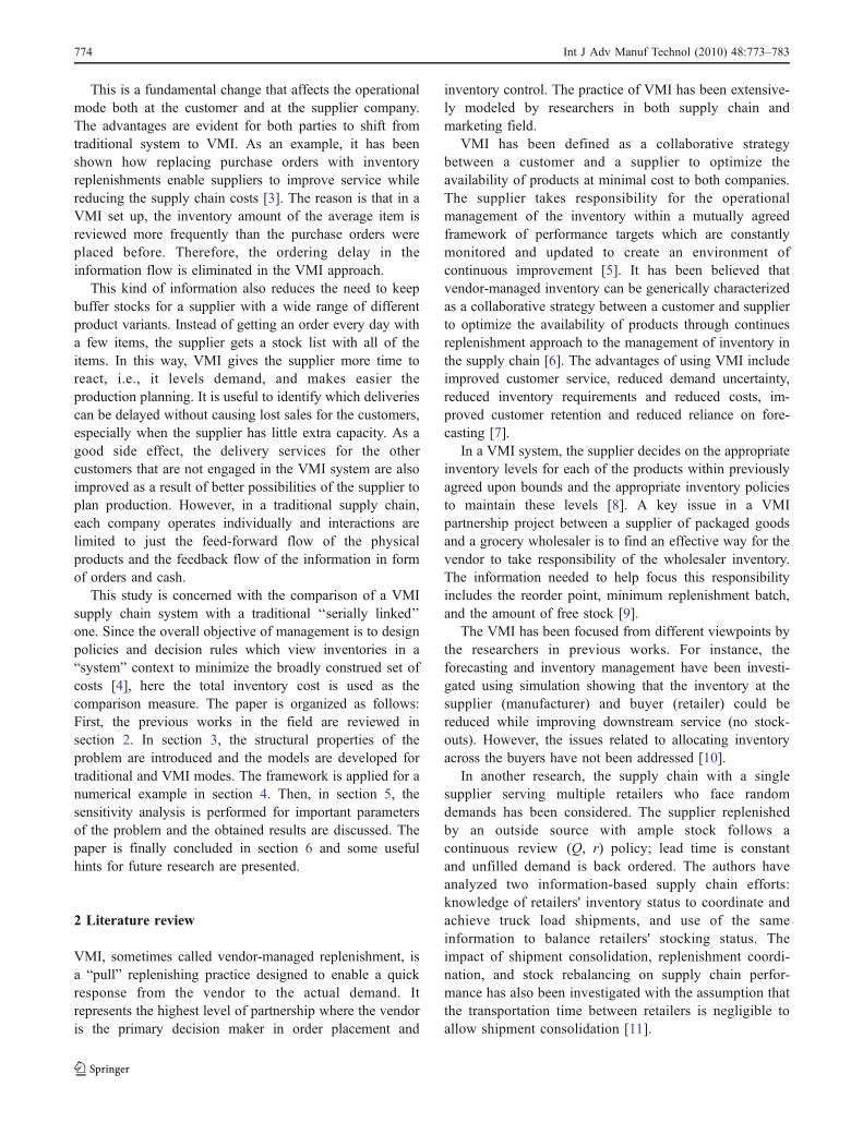
A simple schematic representation of a four echelonsupply chain consisting of a retailer, distributor, warehouseand factory is illustrated in Fig. 1. This structure has beendeveloped as a result of the necessity for a company to bein control of its assets and looking to optimize theirutilization, the cost associated with the transfer of informa-tion and the perceived lack of benefits of this level ofinformation flow [21].

As the supplier and buyer act separately in a traditionalsystem, each party is responsible for controlling of its owninventory. The buyer decides the quantity and timing ofreplenishments and the supplier produces quantitydemanded in an optimal way. When each party makesdecisions independently, the retailer or buyer determinesreplenishment based on minimizing his own operationalcosts. However, since the buyer decisions on timing andquantity neglect the supplier costs, the resulting quantitiesmight not be preferred by the supplier.

Without a VMI agreement, the customer or buyer isresponsible for inventory holding costs, transportationexpenses, ordering charges, the costs of issuing the order,and the costs of receiving those goods. “Issuing the order”relates to writing up the purchase request and determining thesize of order, and thus, it is the cost of having the authorityover replenishment planning. The supplier expenses are thoseof production setup, inventory holding and shipment release.

The average inventory in continuous review model is asfollows:

I ffi Q

2þ r � m ð1Þ

Flow of information upstream

Flow of materials downstream

Distributor Warehouse Factory

Cus

tom

er

Retailer

Fig. 1 The traditional supply chain


where μ is the average demand during the lead time. Thetotal expected cost per time unit for the buyer can bewritten as:

KBTRD :D

QF þ ABð Þ þ hB

Q

2þ r � m

� �þ pDb r; LðQÞð Þ

Q

ð2Þwhere b r; LðQÞð Þ is the average back order of the buyerduring the lead time. After simplify, we have:

KBTRD :D

QF þ ABð Þ þ hB

Q

2þ S

� �þ pDb r; LðQÞð Þ

Qð3Þ

Let us take the derivatives with respect to Q and r andset them to zero:

dKBTRD

dQ: � D

Q2F þ ABð Þ þ hB

2� pDb r; LðQÞð Þ

Q2¼ 0 ð4Þ

dKBTRD

dr: hB þ pD

Q

ddr

b r; LðQÞð Þ ¼ 0 ð5Þ

The Eq. 4 yields the optimal Q for a given reorder pointr as the following:

Q ¼ffiffiffiffiffiffiffiffiffiffiffiffiffiffiffiffiffiffiffiffiffiffiffiffiffiffiffiffiffiffiffiffiffiffiffiffiffiffiffiffiffiffiffiffiffiffiffiffiffiffiffiffiffiffi2D F þ AB þ pb r; LðQÞð Þ� �

hB

sð6Þ

Also, from the Eq. 5 we have:

db r; LðQÞð Þdr

¼ ddr

Z1r

x� rð Þf ðxÞdx ¼ �Z1r

f ðxÞdx ¼ �FðrÞ

ð7Þwhere FðrÞ is the complementary cumulative distribution ofx evaluated at r. Therefore, solving the Eq. 5 with respect tor in terms of Q results in the Eq. 8 as follows:

FðrÞ ¼ hBQ

pDð8Þ

It is assumed that the demand during the lead time isnormally distributed with:

x � N D:Q

Pþ b

� �; s2 Q

Pþ b

� ��

and:

f ðxÞ ¼ 1ffiffiffiffiffi2p

ps

ffiffiffiffiffiffiffiffiffiffiLðQÞp e

�12

x�r

sffiffiffiffiffiLðQÞ

p� 2

ð9Þ

So we have:

b r; LðQÞð Þ ¼Z1r

x� rð Þf ðxÞdx

¼Z1r

x� rð Þ 1ffiffiffiffiffi2p

ps

ffiffiffiffiffiffiffiffiffiffiLðQÞp e

�12

x�r

sffiffiffiffiffiLðQÞ

p� 2

dðxÞ

ð10Þand also:

x� r

sffiffiffiffiffiffiffiffiffiffiLðQÞp ¼ u ) s

ffiffiffiffiffiffiffiffiffiffiLðQÞ

pdu ¼ dx ð11Þ

r � DLðQÞs

ffiffiffiffiffiffiffiffiffiffiLðQÞp ¼ k ) r ¼ ks

ffiffiffiffiffiffiffiffiffiffiLðQÞ

pþ DLðQÞ ð12Þ

After rearranging and simplifying Eqs. 10, 11, and 12 wehave:

b r; LðQÞð Þ ¼ sL

Z1k

u� kð Þ 1ffiffiffiffiffi2p

p e�12u

2du ¼ sLGuðkÞ

¼ s

ffiffiffiffiffiffiffiffiffiffiffiffiffiQ

Pþ b

rL0ðuÞ ð13Þ

where L′(u) is the right hand unit normal linear-lossintegral. The safety stock is calculated by the Eq. 14 asthe following:

S ¼ ksL ¼ ks


Pþ b

rð14Þ

Thus, the expected total cost can be rewritten as:

KBTRD :D

QF þ ABð Þ þ hBQ

2þ hBks


Pþ b

r

þpDs

ffiffiffiffiffiffiffiffiffiffiffiffiQP þ b

qQ

L0ðuÞ ð15Þ

Taking the first derivative of Eq. 15 with regard to orderquantity and set it to zero results in:

dKBTRD

dQ¼ � D

Q2F þ ABð Þ þ hB

2þ hBks

2PffiffiffiffiffiffiffiffiffiffiffiffiQP þ b

q

þ pDsL0ðuÞQ

2PffiffiffiffiffiffiffiQPþb

p �ffiffiffiffiffiffiffiffiffiffiffiffiQP þ b

qQ2

¼ 0

ð16Þ


and after simplifying, we have:

D

Q2F þ AB þ psL0ðuÞ


Pþ b

r" #

¼ hB2

þ hBs


q k þ L0ðuÞFðkÞ

� �ð17Þ

From the Eq. 17, we have:

Q ¼2D F þ AB þ psL0ðuÞ


q� �

hB þ hBs

PffiffiffiffiffiffiffiQPþb

p k þ L0ðuÞFðkÞ

h i2664

3775

12

ð18Þ

And the expected total cost per time unit for the supplieris formulated as follows:

KS ¼ D

QAS þ

hSQ 1� Dp

� 2

ð19Þ

Thus, the total cost per time unit for the supplier and thebuyer together in a traditional supply chain is:

TCTRD ¼ D

QF þ AB þ ASð Þ þ hB

Q

2

þ hBks


pþ b

sþ

pDsffiffiffiffiffiffiffiffiffiffiffiffiQp þ b

qQ

L0ðkÞ

þhs:Q: 1� D

p

� 2

ð20Þ

To find the optimal Q* that minimizes KB, the followingiterative procedure is used:

(1) Calculate Q using this equation: Q ¼ffiffiffiffiffiffiffiffiffiffiffiffiffiffiffiffi2D FþABð Þ

hB

q, and

call this value Q1.(2) Find r from FðrÞby Eq. 8.(3) Calculate L′(u); where it is the right-hand unit normal

linear-loss integral.(4) Use Eq. 16 to calculate a new lot size, Q2.(5) If Q2 � Q1j j ¼ 0, Then,

Calculate TC and go to Step 6.Else,Set Q1 ← Q2 and go to Step 2.

(6) Stop.

3.3 The supply chain with the vendor-managed inventorysystem

Now, the case in which the supplier and buyer have agreedto apply the VMI system is considered. In this case, thesupplier has full information on demand and is responsiblefor managing the inventory for both parties.

The specific VMI scenario considered in this study isdescribed as follows: the supplier in a two-echelon VMIrelationship manages the retailer's or buyer's stock and isprovided with the information on the buyer's sales andstock levels. In this scenario, the buyer does not placeorders on the supplier, and instead, trusts the supplier todispatch the adequate amounts of stock to ensure that thereis enough (but too much) stock at the buyer.

Under the VMI strategy, the vendor takes over the orderingdecision and, hence, the related issuing cost which might notbe the same as what the customer used to pay. A simplediagram of a supply chain with the VMI system is shown inFig. 2. In a VMI system, the supplier (which is often amanufacturer, but may be a distributor) controls the buyer (inthis case a retailer) inventory level, so as to ensure that thepredetermined customer service levels are maintained. Insuch a relationship, the supplier takes the replenishmentdecisions for the buyer and dispatches a quantity of productthat may be fixed (so as to maximize the production ortransport efficiency, for instance) or variable.

Unlike the traditional system, the supplier and buyer in aVMI system act as a single unit. They work based on anagreement which is admitted by both parties. As describedbefore, this agreement is the main idea of VMI and states thatthe supplier establishes and manages the inventory controlpolicies. Here, it is assumed that the supplier pays the ordering

Flow of information upstream

Flow of materials downstream

Distributor Warehouse Factory

Cus

tom

er

Retailer

Fig. 2 A supply chain with a VMI system

D 1,800 units per time unit

σ 3 units

P 3,200 units per time unit

F $ 100

AB $ 80

AS $ 160

hB $ 6 unit per time unit

hS $ 7 unit per time unit

π $ 100

b 0.01 time unit

Table 1 The characteristics ofthe numerical example


and holding costs on behalf of the buyer as a part of thementioned agreement. So, the buyer pays no cost and we have:

KBVMI ¼ 0 ð21ÞThis assumption has also been taken into considerations

in a prior study where supply chain integration in VMI hasbeen discussed [28].

The total cost for the supplier is then expressed asfollows:

KSVMI ¼ D

QF þ AB þ ASð Þ þ hB

Q

2þ hS

Q

2

� 1� D

P

� �þ hBks


Pþ b

r

þpDs


qQ

L0ðuÞ ð22Þ

Thus:

TCVMI ¼ KSVMI ð23ÞThen, the derivative with respect toQ is taken and set to zero.

dTCVMI

dQ¼ � D

Q2F þ AB þ ASð Þ þ hB

2þ hBks


q

þ pDsL0ðuÞQ

2PffiffiffiffiffiffiffiQPþb

p �ffiffiffiffiffiffiffiffiffiffiffiffiQP þ b

qQ2

þ hS 1� DP

�2

ð24Þ

D

Q2F þ AB þ AS þ psL0ðuÞ


Pþ b

r" #

¼ hB2

þ hBs

2PffiffiffiffiffiffiffiffiffiffiffiffiQp þ b

q k þ L0ðuÞFðkÞ

� �þ hs

21� D

P

� �ð25Þ

Table 2 Obtained numerical results for parameter D

Extent point

Table 3 The extent points for important parameters of the problem

Parameter D P F AB AS hB hS

Extentpoint

761.9 7,560 233.5 213.5 91.9 3.4 12.2

0.0%

1.0%

2.0%

3.0%

4.0%

5.0%

6.0%

0 1000 2000 3000 4000

D

Percentage of difference in the total inventory cost in terms of D

0

100

200

300

400

500

600

700

0 1000 2000 3000 4000

Q

D

Quantity of Q in terms of D

Q VMI Q trd

α

Fig. 3 Percentage of difference in the total inventory cost andchanges in the quantity of Q with respect to D


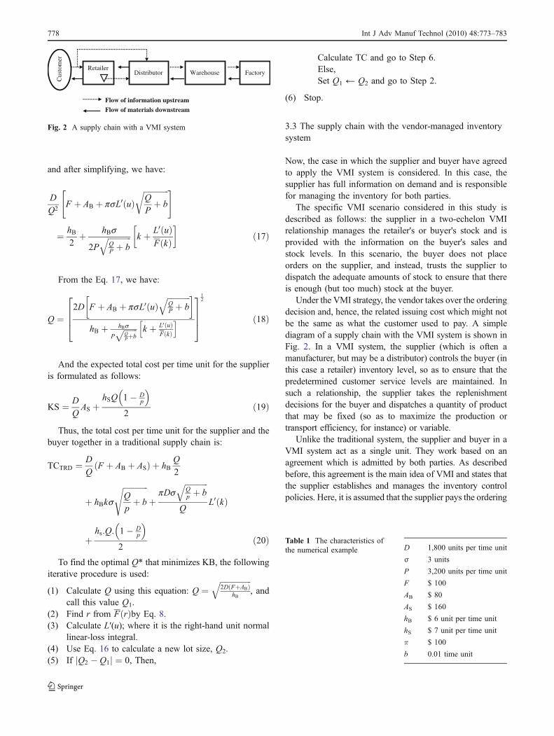
Rearranging and simplifying Eq. 25 results in:

Q ¼2D F þ AB þ AS½ þ psL0ðuÞ


qhB þ hBs

PffiffiffiffiffiffiffiQPþb

p k þ L0ðuÞFðkÞ

h iþ hs 1� D

P

�2664

3775

12

ð26Þ

This value of Q results in minimizing the totalinventory cost of the supplier and buyer in the system.To find the optimal Q*, which minimizes TCVMI orKSVMI, the iterative procedure described in section 3.2 isused, but in the first step, Q is calculated with thefollowing equation:

Q ¼ffiffiffiffiffiffiffiffiffiffiffiffiffiffiffiffiffiffiffiffiffiffiffiffiffiffiffiffiffiffiffiffiffiffiffi2D F þ AB þ Asð ÞhB þ hs 1� D

P

�s

ð27Þ

4 Numerical example

The approach presented in this paper is illustrated with anumerical example given in Table 1. The optimal values(QVMI, QTRD, α) corresponding to each strategy are calculat-

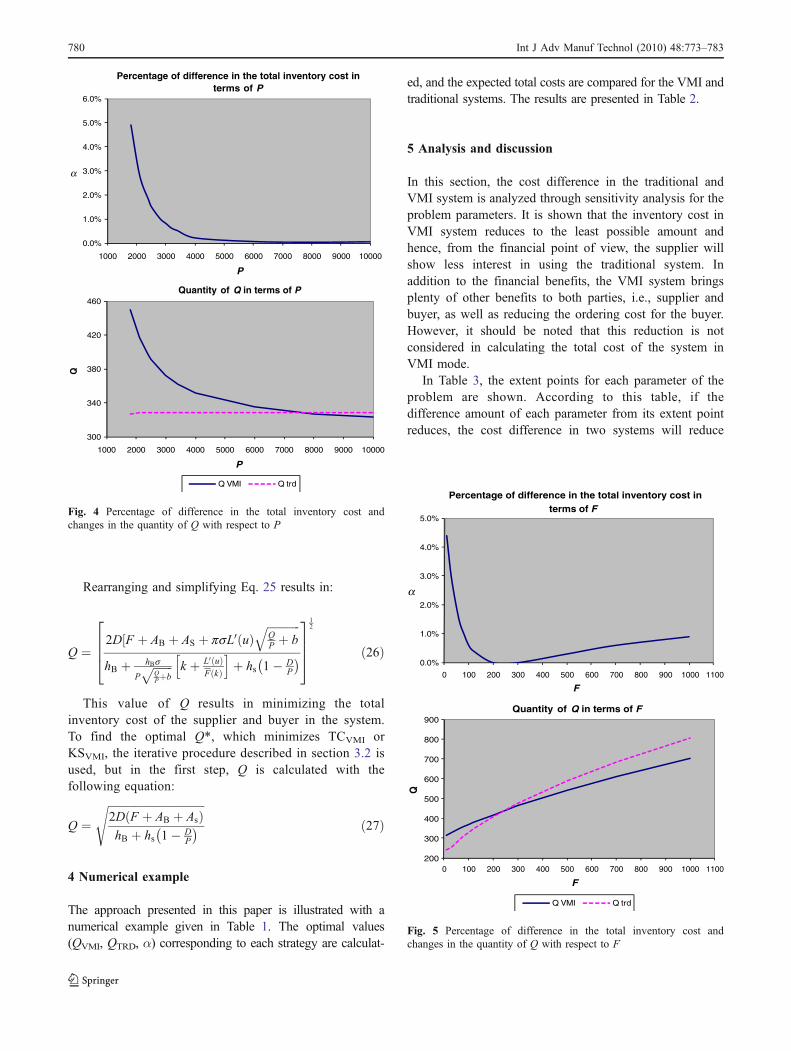
ed, and the expected total costs are compared for the VMI andtraditional systems. The results are presented in Table 2.

5 Analysis and discussion

In this section, the cost difference in the traditional andVMI system is analyzed through sensitivity analysis for theproblem parameters. It is shown that the inventory cost inVMI system reduces to the least possible amount andhence, from the financial point of view, the supplier willshow less interest in using the traditional system. Inaddition to the financial benefits, the VMI system bringsplenty of other benefits to both parties, i.e., supplier andbuyer, as well as reducing the ordering cost for the buyer.However, it should be noted that this reduction is notconsidered in calculating the total cost of the system inVMI mode.

In Table 3, the extent points for each parameter of theproblem are shown. According to this table, if thedifference amount of each parameter from its extent pointreduces, the cost difference in two systems will reduce

0.0%

1.0%

2.0%

3.0%

4.0%

5.0%

6.0%

1000 2000 3000 4000 5000 6000 7000 8000 9000 10000

P

Percentage of difference in the total inventory cost in terms of P

300

340

380

420

460

1000 2000 3000 4000 5000 6000 7000 8000 9000 10000

Q

P

Quantity of Q in terms of P

Q VMI Q trd

α

Fig. 4 Percentage of difference in the total inventory cost andchanges in the quantity of Q with respect to P

0.0%

1.0%

2.0%

3.0%

4.0%

5.0%

F

Percentage of difference in the total inventory cost in terms of F

200

300

400

500

600

700

800

900

0 100 200 300 400 500 600 700 800 900 1000 1100

0 100 200 300 400 500 600 700 800 900 1000 1100

Q

F

Quantity of Q in terms of F

Q VMI Q trd

α

Fig. 5 Percentage of difference in the total inventory cost andchanges in the quantity of Q with respect to F


consequently and if this difference amount increases, thecost difference will increase. It should be noted that if theextent point for a parameter is negative, then by increasingor reducing the value of the parameter, the cost in twotraditional and VMI systems, will never balance. Therefore,the VMI system will always have lower inventory andordering cost compared with the traditional system. As anexample, the extent point value of demand parameter inTable 1 is considered (761.9). The cost difference value inthe two systems is shown in Table 2 for different amountsof demand parameter (D). The results show that if the valueof parameter D approaches to its extent point, the costdifference will reduce and if the value of parameter D getsaway from its extent point, then the cost difference in thetwo systems will increase.

Therefore, it is inferred that if the resulting extent pointis more than its parameter value, increasing the parametervalue will cause to reduce the cost difference in twosystems as long as it touches the extent point. Moreover,reducing the parameter value will cause to increase the costdifference in two systems and vice versa. The impact ofeach related parameter on the percentage of difference in

the total inventory cost of the supply chain (α) and theobtained Q is shown in Figs. 3, 4, 5, 6, 7, 8, and 9. Asshown in these figures, in the points where the quantity ofQ in both traditional and VMI modes are balanced, thedifference in supply chain inventory costs touches the leastamount. Hence, the value of each parameter of the problemwhich results in the least amount of cost difference in twosystems can be calculated as given in Table 3.

In the above figures, it is considered that the costdifference in two traditional and VMI systems are balancedin some points; but this will never occur in practice,because the ordering cost of the buyer which is the supplierduty in VMI mode will reduce considerably as discussed inthe numerical example. This reduction is not exactlyknown, so the ordering cost in traditional mode isconsidered in the VMI mode, too. If the new ordering cost(Ab-VMI<Ab-TRD) is embedded in the model, the costs in twosystems will never balance.

Moreover, in points which the cost difference touchesthe least amount, changing the value of the problemparameters causes to increase the cost difference again. It

0.0%

0.5%

1.0%

1.5%

2.0%

2.5%

0 100 200 300 400 500 600 700 800

AB

Percentage of difference in the total inventory cost in terms of AB

200

300

400

500

600

700

800

0 200 400 600 800

Q

AB

Quantity of Q in terms of AB

Q VMI Q trd

α

Fig. 6 Percentage of difference in the total inventory cost andchanges in the quantity of Q with respect to AB

0.0%

1.0%

2.0%

3.0%

4.0%

5.0%

6.0%

7.0%

8.0%

0 10 20 30 40 50 60 70 80 90 100 110

hB

Percentage of difference in the total inventory cost in terms of hB

0

150

300

450

600

750

900

0 10 20 30 40 50 60 70 80 90 100 110

Q

hB

Quantity of Q in terms of hB

Q VMI Q trd

α

Fig. 7 Percentage of difference in the total inventory cost andchanges in the quantity of Q with respect to hB


shows the reduction in costs for VMI mode comparing withthe traditional mode. Hence, it can be concluded that theVMI system will result in lower cost in all conditions whenthe supplier encounters only one purchaser or buyer incomparison with the traditional system.

6 Conclusions

In this paper, the performance of the VMI system with thesupply chain in traditional mode has been investigatedcomparatively. Mathematical modeling has been applied toderive the total inventory cost as the performance measure.Since none of the previous works quantitatively directed thepractitioners to select the VMI or traditional system, theextent point has been introduced in which the difference oftotal cost in both systems is minimal. The concept has beenapplied to investigate how increasing or reducing therelated parameters changes the total cost of two systemswith respect to each other. A numerical example andsensitivity analysis have been provided to illustrate the

theory and derive the extent points and percentage ofdifference in total cost of both systems. It has been provedthat the VMI system is more beneficial for the coordinationsystem and delivers lower cost in all conditions includingback order. In addition, as one goes farther from the extentpoint, the application of VMI is more justified. The extentpoint can be applied in different practical environments/industries to help practitioners to employ the optimalsupply strategies.

For future research, the new model in which one supplierfaces two or more buyers should be focused. The model inwhich the shortage is in the form of lost sale for the buyershould be also investigated and the conditions in which theVMI system will work better with respect to the traditionalmode should be identified. It is also suggested to considerand analyze the problem presented in this paper in thethree-level mode.

Acknowledgments We would like to express our appreciation forthe University of Tehran (Grant number 8108023/1/08) for thefinancial support of this study. We are also much grateful to therespected reviewers for their valuable comments in preparation of therevised manuscript.

0.0%

1.0%

2.0%

3.0%

4.0%

5.0%

6.0%

7.0%

8.0%

0 100 200 300 400

AS

Percentage of difference in the inventory cost in terms of AS

0

100

200

300

400

500

600

0 100 200 300 400

Q

AS

Quantity of Q in terms of AS

Q VMI Q trd

α

Fig. 8 Percentage of difference in the total inventory cost andchanges in the quantity of Q with respect to AS

0.0%

1.0%

2.0%

3.0%

4.0%

5.0%

6.0%

7.0%

0 5 10 15 20 25 30 35 40 45

hS

Percentage of difference in the inventory cost in terms of hS

0

100

200

300

400

500

0 5 10 15 20 25 30 35 40 45

Q

hS

Quantity of Q in terms of hS

Q VMI Qtrd

α

Fig. 9 Percentage of difference in the total inventory cost andchanges in the quantity of Q with respect to hS


References

1. Sharma S (2009) A composite model in the context of aproduction-inventory system. Optimization Letters 3:239–251

2. Magee JF (1958) Production planning and inventory control.McGraw-Hill Book Company, New York, pp 80–83

3. Waller M, Johnson ME, Davis T (1999) Vendor-managedinventory in the retail supply chain. J Bus Logist 20:183–203

4. Sharma S, Sadiwala CM (1997) Effects of the lost sales oncomposite lot sizing. Comput Ind Eng 32:671–677

5. James R, Rich N, Francis M (1997) Vendor-managed inventory: aprocessual approach, Proceedings of the 6th International IPSERAConference, Ischia, Italy, 24–26 March 1997

6. James R, Francis M, Rich N (2000) Vendor-managed inventory(VMI): a systemic approach. In: value stream management,strategy and excellence in the supply chain. Financial Times/Prentice Hall, Harlow, pp 335–357

7. Fox ML (1996) Integrating vendor-managed inventory into supplychain decision-making, APICS 39th International ConferenceProceedings, New Orleans, pp 126–128

8. Simchi-Livi D, Kaminsky P, Simchi-Livi E (2000) Designing andmanaging the supply chain: concepts, strategies, and case studies.McGraw-Hill, Singapore

9. Holmstrom J (1998) Business process innovation in the supplychain: a case study of implementing vendor-managed inventory.Eur J Purch Supply Manag 4:127–131

10. Cachon G, Fisher M (1997) Campbell soups continuous replen-ishment program: evaluation and enhanced inventory decisionrules. Prod Oper Manag 6:266–276

11. Cheung KL, Lee HL (2002) The inventory benefit of shipmentcoordination and stock rebalancing in a supply chain. Manag Sci48:300–306

12. Gavirneni S (2001) Benefits of co-operation in a productiondistribution environment. Eur J Oper Res 130:612–622

13. Lee HL, Padmanabhan V, Whang S (1997) The bullwhip effect insupply chains. Sloan Manage Rev 38:93–102

14. Chen F, Drezner Z, Ryan JK, Simchi-Levi D (2000) Quantifyingthe bullwhip effect in a simple supply chain: the impact offorecasting, lead times and information. Manag Sci 46:436–443

15. Disney SM, Towill DR (2003) Vendor-managed inventory andbullwhip reduction in a two-level supply chain. Int J Oper ProdManage 23:625–651

16. Disney SM, Towill DR (2003) The effect of vendor-managedinventory (VMI) dynamics on the bullwhip effect in supply chain.Int J Production Economics 85:199–215

17. Xu K, Dong Y, Evers PT (2001) Towards better coordination ofthe supply chain. Transp Res Part E: Logist Trans Rev 37:35–54

18. Aviv Y, Federgruen A (1998) The operational benefits ofinformation sharing and vendor-managed inventory (VMI) pro-grams. Working paper. Washington University, St. Louis

19. Tyan J, Wee HM (2003) Vendor managed inventory (VMI): asurvey of the Taiwanese grocery industry. Eur J Purch SupplyManag 9:11–18

20. Cachon GP, Fisher M (2000) Supply chain inventory managementand the value of shared Information. Manag Sci 46:1032–1048

21. Disney SM, Potter AT, Gardner BM (2003) The impact of vendor-managed inventory on transport operations. Transp Res 39:363–380

22. Tersine RJ, Barman S, Morris JS (1992) A composite EOQ modelfor situational decomposition. Comput Ind Eng 22:283–295

23. Jong JF, Wee HM, Chung CJ (2008) A near optimal solution forintegrated production inventory supplier-buyer deteriorating modelconsidering JIT delivery batch. Int J Comput IntegrManuf 21:289–300

24. Wee HM, Yang PC (2007) A mutual beneficial pricing strategy ofan integrated vendor-buyers inventory system. Int J Adv ManufTechnol 34:179–187

25. Yang PC, Wee HM, Hsu PH (2008) Collaborative vendor-buyerinventory systemwith decliningmarket. Comput Ind Eng 54:128–139

26. Lee H, So K, Tang C (2000) The value of information sharing in atwo-level supply chain. Manag Sci 46:626–643

27. Sterman J (1989) Modeling managerial behavior: misperceptionsof feedback in a dynamic decision making experiment. Manag Sci35:321–339

28. Yao Y, Evers PT, Dresner ME (2007) Supply chain integration invendor-managed inventory. Decis Support Syst 43:663–674


Documents

Developing a two-echelon mathematical model for a vendor-managed inventory (VMI) system