Proceedings of 2013 IAHR World Congress

ABSTRACT: Despite the large studies on flow in partly vegetated open channels, this issue remains of

fundamental importance to better understand the deep relationship between the flow behaviour and the

vegetation structure. This study presents new observations on the boundary layer development, the

turbulence structures and the flow momentum exchange at the interface between flow and vegetation. A

large series of experiments was carried out in a physical model of a very large rectangular channel with

presence of array of vertical, rigid, circular and rough steel cylinders. The array of cylinders was partially

mounted on the bottom of the channel, in the central part, leaving two lateral areas of free flow circulation

near the walls. The three-dimensional flow velocity components were measured using a 3D Acoustic

Doppler Velocimeter ADV.

KEY WORDS: Partly vegetated open channels, Velocity measurements, Turbulence, Boundary layer.

1 INTRODUCTION

In a natural environment, the aquatic vegetations are of different characteristics. They appear as

submerged or emerged, rigid or flexible, leafed or leafless, have branches or rods, and with high or low

density. In addition, the vegetation can occupy the entire width or just part of the stream, leading to

different features of the flow disturbances. Due to the complex structures of vegetation canopies, an

overall understand of all properties of their interaction with the stream flow remains a challenge for

scientists. Shucksmith et al. (2011) indicated that data collected from real channels with live vegetation is

difficult to interpret because of the challenges of measuring the vegetation properties and channel slope.

Thus, to simplify this fact, engineering focused laboratory studies have produced robust models that

describe the resistance within an array of artificial rigid vegetation elements.

Laboratory studies with rigid vegetation neglect some of the important variables introduced by the

presence of natural vegetation (e.g., plant flexibility or the effects of plant growth). Therefore, several

other studies have been carried out taking into account the vegetation flexibility parameters, which are

difficult to measure (e.g., Carollo et al. 2002; Ghisalberti and Nepf, 2002). In order to attain other details

about the natural vegetation effect on flow structure, Shucksmith et al. (2011) conducted an experimental

study using live vegetation grown within a laboratory channel. The authors observed that the addition of

live vegetation to a channel increased its bulk flow resistance as function of the vegetation grew. Other

studies (e.g., Jarvela, 2002, Wilson et al., 2008) have sought to characterize the interaction of different

natural vegetation types with the surrounding flow. In addition to the large range of vegetation typology,

other characteristics should be taken in consideration such as the flow Reynolds number, the canopy

density, and the submergence ratio. For the study of a vegetated channel, such characteristics are just a

Development of lateral boundary layer and turbulent flow

structures at channel-vegetation interfaces

Mouldi Ben Meftah

Professor, Dept. of Civil, Environmental, Building Engineering and Chemistry, Technical University of

Bari,Via E. Orabona 4, 70125 Bari, Italy. Email: m.ben.meftah@poliba.it

Francesca De Serio

Professor, Dept. of Civil, Environmental, Building Engineering and Chemistry, Technical University of

Bari,Via E. Orabona 4, 70125 Bari, Italy. Email: f.deserio@poliba.it

Michele Mossa

Professor, Dept. of Civil, Environmental, Building Engineering and Chemistry, Technical University of

Bari,Via E. Orabona 4, 70125 Bari, Italy. Email: m.mossa@poliba.it

Antonio Felice Petrillo

Professor, Dept. of Civil, Environmental, Building Engineering and Chemistry, Technical University of

Bari,Via E. Orabona 4, 70125 Bari, Italy. Email: a.petrillo@poliba.it

2

few of the key parameters that influence the spatial variability of the flow, momentum transfer, vortex

shedding and dissipation, and instantaneous stresses that are known to affect sediment and morphological

processes in rivers (Neary et al., 2012).

Natural channels are commonly characterized by a main channel for primary flow conveyance and

an overbank, or floodplain, with diminished conveyance capacity and/or flood storage area. Previous

efforts to estimate the flow resistance in compound channels have focused on the boundary shear force

and gravitational force that exist at the main channel-floodplain interface. However, the flow resistance

that develops at the interface is also a function of the turbulence or momentum transfer (Thornton et al.,

2000). At the interface between the vegetated and non-vegetated domains, the transfer of momentum

takes the form of an apparent shear stress (Naot et al., 1996; Ghisalberti and Nepf, 2004; White and Nepf,

2007). But, can all the flow characteristics, in the interface region, be represented by a single parameter?

The free shear layer, formed at the vegetated and non-vegetated interface, is subjected to lateral motion

and may be shifted away from the geometrical edge of the vegetated part (Naot et al., 1996). The

longitudinal vorticity source, that is attenuated within the vegetated domain, is increased externally to this

domain leading to an overall increase in the effects of secondary currents at the main channel. Moreover,

the authors observed a displacement of discharge from the vegetated domains into the clear main channel.

Xiaohui and Li (2002) also indicated the occurrence of significant mass and momentum exchange at the

interface between the vegetated and non-vegetated domains leading to the formation of large eddies.

In the non-vegetated region, flow features resemble those of boundary layer, whereas in the

vegetated region the flow has the features of “porous media”. The flow transition between the two regions

depends strongly on the density and distribution of the vegetation. If there is not enough continuity (i.e.,

the case of densely vegetation) between the flow inside and outside the vegetated area, the flow transition

is sharp. Alternatively, if there is a sufficient degree of continuity, that is the case of low vegetation

density, the flow variables gradually change between the free-fluid and the “porous media” (Pokrajac and

Manes, 2008). Recently, many researchers (e.g., Hsieh and Shiu, 2006; Huai et al., 2011) introduced the

theory of poroelasticity to the study of water flows passing over or next to a vegetated area. The

importance of such a study is that it takes in consideration the effects of the secondary current in addition

to the resistance of vegetation.

Many experimental and numerical studies (Nezu and Onitsuka, 2001; Xiaohui and Li, 2002;

Ghisalberti and Nepf, 2004; White and Nepf, 2007) indicated the formation of coherent vortex structures

at the interface between the vegetated and non-vegetated domains. This is due to the hydrodynamic

instability caused by the mass and momentum exchange relative to the transverse velocity gradient. The

vortexes grow in size and are then transported downstream when their sizes are sufficiently large. The

formation of vortex also causes a decrease in pressure and hence a depression of water surface (Xiaohui

and Li, 2002).

According to White and Nepf (2007), at the interface between the vegetated and non-vegetated

domains, the shear layer is found to possess two distinct length scales. The inner-layer thickness is set by

the array resistance. The wider outer region, which resembles a boundary layer, has a width set by the

water depth and bottom friction. For the case of submerged vegetation, for example, Ghisalberti and Nepf

(2004) observed that in contrast to free shear layers, which grow continuously downstream, the shear

layers generated by submerged vegetation grow only to a finite thickness. In fact, these shear layers are

characterized by coherent vortex structures and rapid vertical mixing, so their thickness controls the

exchange between the vegetation and the overlying water.

Since the vegetation has a large environmental benefit, its incorporation in engineering design is of

fundamental importance. As an example, planting of random or regular arrays of trees can be used as a

protection and management system of floodplains and banks. For this reason, it is important to know the

forces that the flowing river water exerts on the vegetation. Despite significant studies, it was observed

that there still exists a lack of a scientifically robust practical method for the determination of momentum

exchange between the vegetated and non-vegetated zones. In the present study we try to understand some

hydrodynamic characteristics of a partly vegetated channel flow.

3

2 THEORETICAL APPROACH

Along the transversal direction, the turbulent flow in partially vegetated rectangular channels can be

divided into two sub-regions, the vegetated region and the non-vegetated region. In the case where the

mean flow depth, H, is much smaller than the mean channel width, B, that is H/B<<1, the flow can be

considered, approximately, bi-dimensional (x,y), in which x and y are the longitudinal and transversal

directions, respectively. In the present study, the vegetated region was simulated by an array of vertical

steel cylinders. Cylinders were arranged regularly and spaced longitudinally, sx, and transversally, sy, with

the same distance s = sx = sy (see Figure 1). The volume solid fraction of the cylinders is defined as: =

ad/4, where a( = nd) is the total frontal area (area exposed to the flow) per unit array, d is the cylinder

diameter and n is the density of cylinders per unit surface. The porosity of the vegetated zone is N = 1 - .

The velocity inside the vegetated region (defined as a time and spatially average pore velocity) was

defined as Uv. Through the shear layer region across the interface, the flow velocity gradually increases to

reach a maximum and constant velocity Uc in the main channel. The velocity distribution is characterized

by two length scales: v, a length scale over which momentum penetrates into the array and defined as the

inner-layer width (White and Nepf, 2007), and c, a length scale over which the shear extends into the

main channel and defined as the outer-layer width (see Figure 1).

U(y)

Uc

c

ym

v

y=0

Zone similar to a laminar

boundary layer development

Zone of turbulent

Boundary layer development

Uv

Channel wall

Channel axis

x

y Um

U0

sx

sy

X

Y/

2b

B/

2

Figure 1 Problem description at the interface between the vegetated and non-vegetated domains. Note: b is the width

of the non-vegetated area, X and Y are the longitudinal and transversal lengths of the vegetated area, U0 is the mean

channel velocity upstream of the vegetated area, and ym (at which the velocity is indicated by Um) is defined as the

effective boundary layer origin of c

The time-averaged continuity and Navier-Stokes equations of the flow within the array of cylinders

(N = 1) are as follow (using index notation):

0i

i

U

x

(1)

2

2

j i ijii i

j i j j

U U UPg D

x x x x

(2)

4

where xi = (x, y) is the direction tensor, Ui = (U, V) is the time-averaged velocity tensor, in which U and V

are the velocity along x and y, respectively, is the water density, P is the pressure force, is the water

viscosity, gi is the gravitational acceleration tensor, ij is the shear stress tensor and Di is the vegetation

drag force tensor, i.e., the resistance due to the solid medium. ij and Di are defined as:

' 'ij i ju u (3)

1

2i D i iD C aU U (4)

CD is the drag coefficient within the array of cylinders and the symbol | | denotes the vector norm. The

instantaneous velocity is defined as ui(t) = Ui + ui’(t), where ui’ = (u’, v’) is the velocity fluctuation tensor,

in which u’ is the fluctuation of u and v’ is the fluctuation of v.

Averaging eq. (2) over the flow depth, we obtain the momentum equation along the x-direction in

the case of steady and uniform developed turbulent flow (/x = 0). In eq. (5), we define the

depth-average velocity as: Uiz = Ui(z) - Ui’(z), where the symbol z denote the average over the

z-direction (vertical direction) and Ui’ is the depth velocity fluctuation.

2

0 2

' '' 'z z z z z

x

u vU V U U VgS D

y y y y

(5)

where S0 is the energy slope.

In this study, we only focus on the flow motion at the non-vegetated area. In this area, the drag force

due to the array of cylinder is null and thus should be dropped from eq. (5). In addition, it was observed

that the vertical dispersive stress U’V’z is O(0). Because the flow is full turbulent, the stress due to the

viscous term can be ignored from eq. (5). Taking into consideration the contribution of the secondary

circulation, in the boundary layer outside the array of cylinders, eq. (5) becomes:

0

' 'z z z

u vU VgS

y y

(6)

For the sake of simplicity, we have assumed that the secondary flows are related to inertia (Ervine et

al., 2000), which means that

2

z z zU V L U (7)

where L is the secondary current intensity coefficient. In our experiments, it was observed that the value

of L can be considered constant over y ym and then eq. (6) becomes as follows:

2

0

' ' z z

m

u vL UgS y y

y y

(8)

Outside the array of cylinders, it was observed that the magnitude of the mean velocity Uz is almost

equal to that of U at z/H = 0.5 with an error O(-1%). Hence, the mean flow characteristics can roughly be

represented by the flow at mid-depth. Hereafter, for the sake of simplicity, we will address to the flow

velocity U, at z/H = 0.5, rather than the mean velocity Uz. With the assumption of an appropriate eddy

viscosity, ' 'u v = t U/y, and rescale the velocity and the length variables in the following way:

* * and m m

c m c

U U y yU y

U U

(9)

5

With these assumptions and after some simplifications, we obtain from eq. (8) the following final

dimensionlessed expression:

**2 * *

1 2 3*

1

02 2

*

3 *

10

2

where 1

m

t

m

c m

c

c m

t y y

c c m

t

t

ULU U y

Re y

UL

U U

gS

U U

U

Re y

U URe

(10)

In eq.(10), Ret is the Reynolds number based on the outer boundary layer thickness c and the eddy

viscosityt.

3 STUDY METHODS

The experimental runs were carried out in a smooth horizontal rectangular channel at the Coastal

Engineering Laboratory (L.I.C.) of the Department of Civil, Environmental, Building Engineering and

Chemistry at the Technical University of Bari, Italy. The channel consisted of a base and lateral walls

made of glass. The channel is 15 m long, 4 m large and 0.4 m deep. To create a current inside the channel,

a closed hydraulic circuit was constructed. The water was pumped, from a large downstream metallic

tank, by means a Flygt centrifugal electro-pump to the upstream steel tank. A side-channel spillway with

adjustable height made from different plates mounted together was fitted into the upstream tank. The

water that overflowed was discharged into the large metallic tank located downstream of the channel.

Two different electromagnetic flow meters were mounted onto the hydraulic circuit of the channel, in

order to measure both the pumped and the overflowed flow rates. The channel discharge Q was

determined as the difference between the two flow rates. To create a smooth flow transition from the

upstream tank to the flume, a set of stilling grids were installed in the upstream tank to dampen inlet

turbulence. The upstream and downstream gates were used to define the flow depth and mean velocity in

the channel (Figure 2).

The model array was constructed of vertical, rigid, circular and threaded steel cylinders. The

cylinder height, h, and diameter, d, were 0.31 m and 0.003 m, respectively. The cylinder extremities were

inserted into a plywood plaque 3.0 m long, 4.0 m wide and 0.02 m thick, which in turn was fixed along

the channel bottoms, forming the experimental area of 3x3 m. It should be taken into account that the

arrays of cylinders were partially mounted on the bottom of the channel, in the central part, leaving two

lateral areas, each of them is 0.5 m large, of free flow circulation near the walls. The plywood plaque was

extended 3 m both upstream and downstream of the array of cylinders (experimental area) and was

tapered to the channel bottom to minimise flow disturbance. Cylinders were arranged regularly and

spaced longitudinally, sx, and transversally, sy, with the same distance sx = sy = 5.0 cm, so that the cylinder

density, n, was 400 cylinders/m2.

The origin of the x-axis (x = 0) was taken at the leading edge of the array of cylinders, while the

origin of the y-axis (y = 0) was taken at the interface between the vegetated and non-vegetated domains.

Because water is forced to move around the cylinders, the flow within the canopy is turbulent and highly

heterogeneous at the scale of the individual cylinder. Therefore, the instantaneous three-dimensional flow

velocity components, through different longitudinal, cross and horizontal planes, were accurately

measured (1cm x 1cm grid resolution) using a three-dimensional (3D) Acoustic Doppler Velocimeter

(ADV) system, together with CollectV software for data acquisition and ExploreV software for the data

analysis, all produced by Nortek. The ADV was used with a velocity range equal to 0.30 m/s, a velocity

6

accuracy of 1%, a sampling rate of 25 Hz and a sampling volume of vertical extend of 9mm. A 15db

signal-to-noise ratio (SNR) and a correlation coefficients larger than 70% are recommended by the

manufacturer for high-resolution measurements. The acquired data were filtered based on the Tukey’s

method and the bad samples (SNR<15db and correlation coefficient<70%) were also removed. Because

of the configuration of the ADV of downlooking probe probes, the uppermost 7cm of the flow could not

be sampled (Ghisalberti and Nepf, 2004). Additional details concerning the channel setup and the ADV

operation can be found elsewhere in Ben Meftah et al. (2007, 2008 and 2010). The initial experimental

conditions and parameters of the investigated runs are shown in Table 1. The solid fraction of cylinders

was constant for all the experimental runs having a value of = 0.0028.

HU0

x

z

3m 3m3m

Emergent array of cylindersUpstream gate Downstream gate

15m

Plywood plaque

Veg

etat

ed a

rea

Side View

Up View

Sx

Sy

xy

U0

4m

Channel axis

3m

0.5m Non-vegetated area

Non-vegetated area

Figure 2 General sketch of the laboratory flume with the experimental area

Table 1 The initial experimental conditions and parameters of the investigated runs

Runs H

(m)

U0

(m/s)

T

(°C)

Uc

(m/s)

Um

(m/s)

Re0

(-)

Fr0

(-)

Rec

(-)

Frc

(-) Note

R1 0.25 0.100 20 0.193 0.076 25000 0.064 48325 0.123 Re0 = U0H/

Fr0 = U0/(gH)0.5

Rec = UcH/

Frc = Uc/(gH)0.5

R2 0.22 0.114 9 0.217 0.081 17194 0.077 34659 0.148

R3 0.18 0.139 14 0.264 0.097 19555 0.105 40361 0.199

R4 0.14 0.179 15 0.342 0.132 20163 0.152 41932 0.292

T, Re0, Fr0, Rec and Frc, represent water temperature, inlet Reynolds number, inlet Froude number, Reynolds number

in non-vegetated area and Froude number in non-vegetated area.

4 RESULTS AND DISCUSSION

Figure 3 shows an example of the vector maps of the measured longitudinal velocity component U

in both the vegetated and non-vegetated areas. The lateral profiles of U refer to runs R2 and R3. The solid

curve in both examples qualitatively represents the lateral shear-layer growth as function of x. It was

obtained at the position where the longitudinal component of the water velocity U is equal to 0.99 of the

free-stream water velocity outside the boundary layer Uc. The numerous profiles in addition to the

numerous measurement points for each profile, as shown in Figure 3, have been taken in order to get

maximum details on the flow structures inside and outside the array of cylinders.

7

Figure 3 Vector map of the U-velocity distribution for Runs R2 and R3. The solid curve qualitatively represents the

shear-layer growth and it was obtained at U(y) = 0.99Uc.

8

At the entrance section, where x/X is O(0), the U-profile appears of constant value along all the

lateral direction, except in the positions in line with the cylinders, where a reduction of U can be clearly

noted, due to the known wake region formed downstream of each cylinder. As going further downstream

of the entrance section, the magnitude of U starts to decrease gradually within the array of cylinders,

showing a “sawteeth” shape at the entrance region (x/X < 0.3) and a sinusoidal trend further downstream.

Outside the array of cylinders, the U-profiles, at x/X 0.1, are characterized by two typical regions: i) a

region immediately next to the interface between the vegetated and non-vegetated domains in which U

increases continuously from a slip velocity at the interface, defined as Us = U(y = 0) - Uv, to a full velocity

Uc, ii) a free-stream region where U remains almost constant and equal to the full velocity Uc. It can be

noted that, outside the array of cylinders, the flow velocity U behaves in exactly the same way of flow

velocity close to a flat plate (Schlichting, 1955). Hence, By analogy with the flow over a flat plate, the

first region is defined as the sheared region and the second region is called the region of free-stream

velocity. The interface between both regions is called the shear-layer or boundary layer. On the other hand,

it can be seen that both the free-stream velocity Uc and the velocity in the sheared region increase

gradually with increasing distance from the leading edge of the array of cylinders in the downstream

direction. Starting from x/X ≈ 0.5, both U and Uc velocities show slight increase as x increases, tending to

an almost uniform state.

Figure 3 shows that the shear-layer thickness increases along the interface between the vegetated

and non-vegetated domains in the downstream direction. Near the leading edge of the array of cylinders,

at x/X 0.1, the thickness of the shear-layer starts to increase with a slight rate, similar to the classical

laminar boundary layer observed over a flat plate (Schlichting, 1955). From x/X ≈ 0.1 to x/X ≈ 0.4, the

shear-layer thickness shows a clear sharp increase, denoting a transition from laminar-form to turbulent

shear-layer. Further downstream, x/X 0.5, the thickness of the turbulent shear-layer tends to almost a

constant value, where a fully turbulent state is reached.

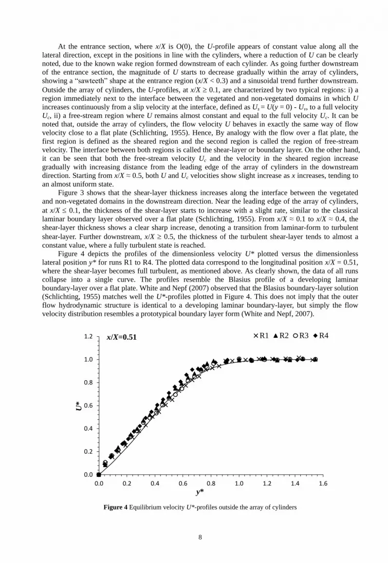
Figure 4 depicts the profiles of the dimensionless velocity U* plotted versus the dimensionless

lateral position y* for runs R1 to R4. The plotted data correspond to the longitudinal position x/X = 0.51,

where the shear-layer becomes full turbulent, as mentioned above. As clearly shown, the data of all runs

collapse into a single curve. The profiles resemble the Blasius profile of a developing laminar

boundary-layer over a flat plate. White and Nepf (2007) observed that the Blasius boundary-layer solution

(Schlichting, 1955) matches well the U*-profiles plotted in Figure 4. This does not imply that the outer

flow hydrodynamic structure is identical to a developing laminar boundary-layer, but simply the flow

velocity distribution resembles a prototypical boundary layer form (White and Nepf, 2007).

0.0

0.2

0.4

0.6

0.8

1.0

1.2

0.0 0.2 0.4 0.6 0.8 1.0 1.2 1.4 1.6

U*

y*

R1 R2 R3 R4x/X=0.51

Figure 4 Equilibrium velocity U*-profiles outside the array of cylinders

9

The solid line in Figure 4 represents a proposed solution of eq. (10) deduced via numerical iterative

methods, with L ≈ 0.1(experimentally proved as almost constant over y), 1 ≈ 0.1, Ret ≈ 360 (t averaged

over y), 2 ≈ 0.5 and 3 ≈ 0, as:

* * *2 *3U tanh y y Cy (11)

where C is a constant of order 0.3. It is worth to note that the proposed solution matches well the

experimental data plotted in Figure 4. This implies the validity of the proposed theoretical approach for

the mean flow velocity distribution outside the array of cylinders.

To better understand the flow hydrodynamic structure in the outer region, we need thorough analysis

about the background turbulence of the flow field. Figure 5, as an example, illustrates the lateral profiles

of the turbulence intensity of the longitudinal velocity component u for all runs. The data always referred

to x/X = 0.51. The turbulence intensity profiles, for all runs, show similar tendencies. Two peaks are

clearly present on the four profiles: i) a peak appears at the interface between the vegetated and the

non-vegetated domains, at the minimum value of y* (≈ -0.1), in good agreement with many studies in

literature (e.g., Nezu and Onitsuka, 2001; White and Nepf, 2007 ), ii) a second peak appears at a certain

distance from the interface between the two domains, for this study, at y* ≈ 0.5.

The second peak of the turbulence intensity was not mentioned in previous studies. This new

observation on the dynamic structure of the flow in the outer region is of high importance. The absence

of a second peak in previous recent studies does not mean that it does not exist, but probably it is confined

to the interface between the vegetated and non-vegetated domains. This may be due to many factors, such

as the small width of the laboratory channels used for previous studies, the small width of both the

non-vegetated and vegetated areas, the width proportionality between the non-vegetated and vegetated

domains and the effect of the vegetation density. It is useful to remember that this experimental study was

carried out in a channel of 4 m wide, with a vegetated area 3m long and 3m wide and a non-vegetated

area of 0.5 m wide (see Figures 1 and 2).

Figure 6 shows the normalized Reynolds stress versus the normalized lateral coordinate in the outer

layer. Similar to Figure 5, the data refer to all runs and to x/X = 0.51. The Reynolds stress was normalized

by its maximum value obtained along y*. The profiles of the Reynolds stress tend to collapse in a single

curve, showing the same trend observed for the turbulence intensity profiles (Figure 5). The two peaks

also appeared in this case, particularly the second one is at y* ≈ 0.5, consistently to what observed in

Figure 5.

0.00

0.01

0.02

0.03

0.04

0.05

0.06

0.07

0.08

0.09

-0.2 0.0 0.2 0.4 0.6 0.8 1.0 1.2 1.4 1.6

y*

R1 R2 R3 R4x/X=0.51

2'

c

u

U

Figure 5 Turbulence intensity distribution in the outer layer

10

-0.2

0.0

0.2

0.4

0.6

0.8

1.0

1.2

-0.2 0.0 0.2 0.4 0.6 0.8 1.0 1.2 1.4 1.6

y*

R1 R2 R3 R4x/X=0.51

max

' '

' '

uv

uv

Figure 6 Reynolds shear stress distribution in the outer layer

5 CONCLUSIONS

This study presents new observations on the boundary layer development, the turbulence structures

and the flow momentum exchange at the interface between a vegetated and non-vegetated domains. A

theoretical model for the mean flow velocity distribution at the outer layer was proposed and

experimentally validated.

Outside the array of cylinders, the U-profiles, at x/X 0.1, are characterized by two typical regions:

i) a region immediately next to the interface between the vegetated and non-vegetated domains in which

U increases continuously from a slip velocity at the interface to a full velocity Uc, ii) a free-stream region

where U remains almost constant and equal to the full velocity Uc. The flow velocity U behaves in exactly

the same way of flow velocity close to a flat plate. The shear-layer thickness increases along the interface

in the downstream direction. A laminar-form, near the leading edge of the array of cylinders, and a

turbulent, further downstream, boundary-layers were distinguished, similarly to the case of the flow over

a flat plate.

Across the full turbulent shear-layer, the profiles of the dimensionless velocity U* plotted versus the

dimensionless lateral position y*, for all runs, collapse into a single curve, resembling the Blasius profile

of a developing laminar boundary-layer over a flat plate. The proposed theoretical approach for the mean

flow velocity distribution outside the array of cylinders was experimentally validated.

The turbulence intensity profiles show two peaks along the transversal direction outside the array of

cylinders: i) a first peak appears at the interface between the vegetated and the non-vegetated domains,

which is in good agreement with many previous studies in literature, ii) a second peak appears at a

distance of y* ≈ 0.5 from the interface, which is a new aspect of the flow features in this region. The

Profiles of the Reynolds stress showed the same trend observed with the turbulence intensity distribution.

ACKNOWLEDGEMENT

The study was carried out at the Coastal Engineering Laboratory (L.I.C) of the Technical University of

Bari, Italy, Department of Civil, Environmental, Building Engineering and Chemistry.

11

References Ben Meftah M., De Serio F., Mossa M. and Pollio A., 2007. Analysis of the velocity field in a large rectangular

channel with lateral shock wave. Environmental Fluid Mechanics, 7(6), 519-536. Ben Meftah M., De Serio F., Mossa M. and Pollio A., 2008. Experimental study of recirculating flows generated by

lateral shock waves in very large channels. Environmental Fluid Mechanics, 8(6), 215-238. Ben Meftah M., Mossa M. and Pollio A., 2010. Considerations on shock wave/boundary layer interaction in undular

hy-draulic jumps in horizontal channels with a very high aspect ratio. European Journal of Mechanics B/Fluids 29, 415-429.

Carollo F.G., Ferro V. and Termini D., 2002. Flow velocity measurement in vegetated channels. Journal of Hydraulic Engineering, 128(7), 664-673.

Ervine D.A., Babaeyan-Koopaei k. and Sellin R.H.J., 2000. Two-dimensional solution for straight and meandering overbank flows. Journal of Hydraulic Engineering, 126(9), 653-669.

Ghisalberti M. and Nepf H.M., 2002. Mixing layers and coherent structures in vegetated aquatic flows. Journal of Geophysical research, 107(C2), (3) 1-11.

Ghisalberti M. and Nepf H.M., 2004. The limited growth of vegetated shear layers. Water resources Research, 40(W07502), 1-12.

Hsieh P.C. and Shiu Y.S., 2006. Analytical solutions for water flow passing over a vegetal area. Advances in Water Resources, 29(9), 1257-1266.

Huai W., Geng C., Zeng Y. and Yang Z., 2011. Analytical solutions for transverse distributions of stream-wise velocity in turbulent flow in rectangular channel with partial vegetation. Applied Mathematics and Mechanics (English Edition), 32(4), 459-468.

Jarvela J., 2002. Flow resistance of flexible and stiff vegetation: a flume study with natural plants. Journal of hydrology, 269, 44-54.

Naot D., Nezu I. and Nakagawa H., 1996. Hydrodynamic behavior of partly vegetated open channels. Journal of Hydraulic Engineering, 122(11), 625-633.

Neary V.S., Constantinescu S.G., Bennett S.J. and Diplas P., 2012. Effects of Vegetation on Turbulence, sediment transport, and stream morphology. Journal of Hydraulic Engineering, 138(9), 765-776.

Nezu I. and Onitsuka K., 2001. Turbulent structures in partly vegetated open-channel flows with LDA and PIV measurements. Journal of Hydraulic Research, 39(6), 629-642.

Pokrajac D. and Manes C., 2008. Interface between turbulent flows above and within rough porous walls. Acta Geophysica, 56(3), 824-844.

Schlichting H., 1955. Boundary layer theory. First English Edition, Pergamon Press, New York, London, Paris. Shucksmith J.D., Boxall J.B. and Guymer I., 2011. Bulk flow resistance in vegetated channels: Analysis of

momentum balance approaches based on data obtained in aging live vegetation. Journal of Hydraulic Engineering, 137(12), 1624-1635.

Thornton C.I., Abt S.R., Morris C.E. and Craig Fischenich J., 2000. Calculating shear stress at channel-overbank interfaces in straight channels with vegetated floodplane. Journal of Hydraulic Engineering, 126(12), 929-936.

Wilson C.A.M, Hoyt J. and Schnauder I., 2008. Impact of foliage on the drag force of vegetation in aquatic flows. Journal of Hydraulic Engineering, 134(7), 885-891. 765-776.

White B.L. and Nepf H.M., 2007. Shear instability and coherent structures in shallow flow adjacent to a porous layer. J. Fluid Mech., 593, 1-32.

Xiaohui S. and Li C.W., 2002. Large eddy simulation of free surface turbulent flow in partly vegetated open channels. International Journal for Numerical Methods in Fluids, 39, 919-937.