Embed Size (px)
Citation preview

Chandrakant S. Desai
Mechanicsof
Materialsand
InterfacesThe
Disturbed State Concept
Boca Raton London New York Washington, D.C.CRC Press
© 2001 By CRC Press LLC

This book contains information obtained from authentic and highly regarded sources. Reprinted materialis quoted with permission, and sources are indicated. A wide variety of references are listed. Reasonableefforts have been made to publish reliable data and information, but the author and the publisher cannotassume responsibility for the validity of all materials or for the consequences of their use.
Neither this book nor any part may be reproduced or transmitted in any form or by any means, electronicor mechanical, including photocopying, microfilming, and recording, or by any information storage orretrieval system, without prior permission in writing from the publisher.
The consent of CRC Press LLC does not extend to copying for general distribution, for promotion, forcreating new works, or for resale. Specific permission must be obtained in writing from CRC Press LLCfor such copying.
Direct all inquiries to CRC Press LLC, 2000 N.W. Corporate Blvd., Boca Raton, Florida 33431, or visitour website at www.crcpress.com
Trademark Notice: Product or corporate names may be trademarks or registered trademarks, and areused only for identification and explanation, without intent to infringe.
© 2001 by CRC Press LLC
No claim to original U.S. Government worksInternational Standard Book Number 0-8493-0248-X
Library of Congress Card Number 00-052883Printed in the United States of America 1 2 3 4 5 6 7 8 9 0
Printed on acid-free paper
Library of Congress Cataloging-in-Publication Data
Desai, C.S. (Chandrakant S.), 1936–Mechanics of materials and interfaces : the disturbed state concept / by Chandrakant S. Desai
p. cm.Includes bibliographical references and index.ISBN 0-8493-0248-X (alk. paper)1. Strength of materials—Mathematical models. 2. Strains and stresses. 3. Interfaces
(Physical sciences) I. Title.
TA405 .D45 2000620.1′12′015118—dc21 00-052883

To my father
• who, I believe, is inquisitive and questioning in the space beyond,which is congruent to that of mine.
and
To those giants
• of mechanics, physics, and philosophy, on whose contributions westand and extend.
Continuum and discontinuum,Points and spaces,Exist together, United and Coupled;Sat and Asat,Existence and nonexistence;Exist together, United and Coupled;Merging in each other.
© 2001 By CRC Press LLC

PREFACE
Understanding and characterizing the mechanical behavior of engineeringmaterials and interfaces or joints play vital roles in the prediction of thebehavior, and the analysis and design, of engineering systems. Principles ofmechanics and physics are invoked to derive governing equations that allowsolutions for the behavior of the systems. Such closed-form or numericalsolutions involve the important component of material behavior defined byconstitutive laws or equations or models.
Definition of the constitutive laws based on fundamental principles ofmechanics, identification of significant parameters, determination of theparameters from appropriate (laboratory and/or field) tests, validation of themodels with respect to the test data, implementation of the models in the solu-tion procedures—closed-form or computational—and validation of practicalboundary-value problems are all important ingredients in the developmentand use of realistic material models.
The characterization of the mechanical behavior of engineering materials,called the stress–strain or constitutive models, has been the topic under thegeneral subject of “mechanics of materials”. As material behavior is veryoften nonlinear, the governing equations are also nonlinear. In the earlystages, however, it was necessary to linearize the governing differential equa-tions so that the closed-form solution procedures could be used. The adventof the electronic computer, with increasing storage capacity and speed, madeit possible to solve nonlinear equations in discretized forms. Hence, the needto assume constant coefficients or material parameters in the linear andclosed-form solutions may no longer exist. As a consequence, it is now pos-sible to develop and use models for realistic nonlinear material response.
Almost all materials exhibit nonlinear behavior. In simple words, this impliesthat the response of the material is not proportional to the input excitation orload. Hence, although the assumption of linearity provided, and still can pro-vide, useful solutions, their validity is highly limited in the nonlinear regimes ofthe material response. Thus, the fact that modern computers and numerical orcomputational methods now permit the consideration of nonlinear responses isindeed a highly desirable development.
Among linear constitutive models are Hooke’s law that defines linear elasticstress–strain response under mechanical load, Darcy’s law that defines the lin-ear velocity-gradient response for fluid flow, and Ohm’s law that defines thelinear voltage-current relation for electrical flow. It is recognized that thevalidity of these models is limited. Hooke’s law does not apply if the materialresponse involves effect of factors such as state of stress or strain, stress orloading paths, temperature, initial and induced discontinuities, and existence
© 2001 By CRC Press LLC

of fluid or gas in the material’s porous microstructure. Darcy’s law does notapply if the flow is turbulent, and Ohm’s law loses validity if the conductingmaterial is nonhomogeneous and thermal effects are present.
For the characterization of the nonlinear behavior of materials, the effectsof significant factors such as initial conditions, state of stress, stress or loadingpath, type of loading, and multiphase nature need to be considered for real-istic engineering solutions. The pursuit of the development of models for thenonlinear response has a long history in the subjects of physics and mechan-ics of materials. Among the models proposed and developed are linear andnonlinear elasticity (e.g., hyper- and hypoelasticity), classical plasticity (vonMises, Tresca, Mohr–Coulomb, Drucker–Prager), continuous hardening oryielding plasticity (critical-state, cap, hierarchical single-surface–HISS), andkinematic and anisotropic hardening in the context of the theory of plasticity.
Viscoelastic, viscoplastic, and elastoviscoplastic models are among thosedeveloped to account for time-dependent viscous or creep response. Endo-chronic theory involving an implicit time scale has been proposed in the con-text of plasticity and viscoplasticity.
Models based on micromechanical considerations involve the idea that theobserved macrolevel response of the material can be obtained by integrating theresponses of behavior at the micro- or particle level, often through a process oflinear integration. Although this idea is elegant, at this time it suffers from thelimitation that the particle-level response is difficult to measure and characterize.
Most of the models are based on the assumption that the material is contin-uous. As a result, the theories of continuum mechanics have been invoked fortheir formulation. It is, recognized, however, that discontinuities exist anddevelop in a deforming material. Thus, the theories based on continuummechanics may not be strictly valid, and various models based on fractureand continuum damage concepts thereby become relevant.
The classical continuum damage models are based on the idea that a mate-rial experiences microcracking and fracturing, which can cause degradationor damage in the material’s stiffness and strength. The remaining degradedstiffness (strength) is then defined on the basis of the response of the undam-aged part modified by growing damaged parts, which are assumed to act likevoids and possess no strength at all. As a result, the classical continuum dam-age models do not allow for the coupling and interaction between the dam-aged and undamaged parts. This aspect has significant consequences, as theeffect of neighboring (damaged) parts is not included in the characterizationof the response.
Various nonlocal and microcrack interaction models have been proposed inthe context of the classical damage model. An objective here has been todevelop constitutive equations that allow for the coupling between the dam-aged (microcracked) and undamaged parts and the effect of what happens inthe neighborhood of a material point. Such enhancements as gradient,Cosserat, and micropolar theories have been proposed to incorporate the non-local effects.
© 2001 By CRC Press LLC

The effects of temperature and other environmental factors are incorpo-rated by developing separate theories or by expressing the parameters in theabove models as functions of temperature or other environmental factors.
The foregoing models are usually relevant for a specific characteristic of thematerial behavior such as elastic, plastic, creep, microcracking, and fracture.Each model involves a set of parameters for a specific characteristic that needsto be determined from laboratory tests. There is a growing recognition thatdevelopment of unified or integrated constitutive descriptions can lead tomore efficient, economical, and simplified models with ease of implementa-tion in solution procedures. As a result, a number of efforts have been madetoward unified or hierarchical models. The approach presented in this bookrepresents one of these unified concepts: the disturbed state concept (DSC).
The DSC is a unified modelling approach that allows, in an integrated man-ner, for elastic, plastic, and creep strains, microcracking and fracture leadingto softening and damage, and stiffening or healing, in a single framework. Itshierarchical nature permits the adoption and use of specialized versions forthe foregoing factors. As a result, its development and application are simpli-fied considerably.
The DSC is based on the basic physical consideration that the observedresponse of a material can be expressed in terms of the responses of its con-stituents, connected by the coupling or disturbance function. In simplewords, the observed material state is considered to represent disturbance ordeviation with respect to the behavior of the material for appropriatelydefined reference states. This approach is consistent with the idea that thecurrent state of a material system, animate or inanimate, can be considered tobe the disturbed state with respect to its initial and final state(s).
In the case of engineering materials, the DSC stipulates that at any givendeformation stage, the material is composed of two (or more) parts. Forinstance, a dry deforming material is composed of material parts in the orig-inal (continuum) state, called the relatively intact (RI) state, and remainingparts in the degraded or stiffened state, called the fully adjusted (FA) state;the meanings of the terms “RI and FA state” will be explained in subsequentchapters. The degraded part can represent effects of relative particle motionsand microcracking due to the natural self-adjustment (SA) of particles in thematerial’s microstructure and can lead to damage or degradation. Under fac-tors such as chemical, temperature, and fluid effects, the microstructure mayexperience stiffening or healing. Although the degradation or damage aspectin the DSC is similar to that in the classical damage models, the basic frame-work of the DSC is general and significantly different from that of the dam-age concept.
If a material element is composed of more than one material, the DSC canbe formulated for the overall observed response (of the composite) by treat-ing the behavior of individual components as reference responses. Thebehavior of an individual component may be characterized by using a con-tinuum theory or by treating it as a mixture of the RI and FA parts.
© 2001 By CRC Press LLC

Details of the DSC, including formulation of equations, identification ofmaterial parameters, determination of parameters from (laboratory) tests,validation at the laboratory test stage, implementation in solution (com-puter) procedures, and validation and solution of practical boundary-valueproblems, are presented in this book. Comparisons between the DSC andother available models are discussed, including the advantages the DSCoffers. The latter arise due to characteristics such as the compact and unifiednature of the DSC, physical meanings of material parameters, considerablereduction in the regression and curve-fitting required in many other models,ease of determination of parameters, and ease of implementation in solutionprocedures.
One of the DSC’s advantages is that it can be used for “solid” materials andfor interfaces and joints. The latter play an important role in the behavior ofmany engineering systems involving combinations of two or more materials.They include contacts in metals, interfaces in soil-medium (structure) prob-lems, joints in rock, and joints in electronic packaging systems. It is shownthat the mathematical framework of the DSC for three-dimensional solidscan be specialized for the behavior of material contacts idealized as thin-layerzones or elements.
The fact that the DSC allows for interaction and coupling between the RIand FA parts offers a number of advantages in that the nonlocal effects areincluded in the model, hence also the characteristic dimension.
The DSC does not require constitutive description of particle-level processesas the micromechanical models do. The interacting behavior of the materialcomposed of millions of particles is expressed in terms of the coupledresponses of the material parts (clusters) in the RI and FA parts. The responseof the RI and FA parts can be defined from laboratory tests. Thus, the DSCeliminates the need for defining particle-level behavior, which is difficult tomeasure at this time. At the same time, it allows for the coupled microlevelprocesses.
The behavior of material parts in the reference states in the DSC can bedefined on the basis of any suitable model(s). Often, such available contin-uum theories as elasticity and plasticity, and the critical-state concept, areinvoked for the characterizations.
The DSC represents a continuous evolution in the pursuit of the develop-ment of constitutive models by the author and his co-workers. Although itinvolves a number of new and innovative ideas, the DSC also relies on theavailable theories of mechanics and the contributions of many people whohave been the giants in this field. For instance, the DSC includes ideas andconcepts from the available elasticity, plasticity, viscoplasticity, damage, frac-ture, and critical-state theories. As the DSC allows adoption of these availablemodels as special cases, they are presented individually in separate chapters,with identification of their use in the DSC.
In summary, the DSC is considered to represent a unique and powerful mod-elling procedure to characterize the behavior of a wide range of materials and
© 2001 By CRC Press LLC

interfaces. Its capabilities go beyond available material models, and it simulta-neously leads to significant simplification toward practical applications.
The DSC permits approximation of material systems as discontinuous andincludes their continuum attribute as a special case. Thus, it can provide ageneralized basis for the introduction of the subject of mechanics of materials.It is therefore possible that the DSC can be introduced first as the general andbasic approach in undergraduate courses on the strength or mechanics ofmaterials in the first few lectures, and then the traditional mechanics ofmaterials can be taught as before, by assuming the material systems to becontinuous. The DSC can later be brought into the upper-level undergradu-ate courses. Hence, the material in this book can be introduced in under-graduate courses.
The advanced topics in the book can be taught in graduate-level courseswith prerequisites of continuum theories such as elasticity and plasticity. Thebook can be useful to the researcher who wants to employ up-to-date, unifiedand simplified models to account for realistic nonlinear behavior of materialsand interfaces. It will also be useful to practitioners involved in the solutionof problems requiring realistic models and computer procedures.
The objectives of this text are as follows:
(1) to present a philosophical and detailed theoretical treatment of theDSC, including a comparison with other available models;
(2) to identify the physical meanings of the parameters involved andpresent procedures to determine them from laboratory test data;
(3) to use the DSC to characterize the behavior of materials such asgeologic, ceramic, concrete, metal (alloys), silicon, and asphalt con-crete, and interfaces and joints;
(4) to validate the DSC models with respect to laboratory tests usedto find the parameters, and independent tests not used in the cali-bration;
(5) to implement the DSC models in computer (finite-element) proce-dures; and
(6) to validate the computer procedures by comparing predictionswith observations from simulated and field boundary-value prob-lems.
The basic theme of the text is to show that the DSC can provide a unifiedand simplified approach for the mathematical characterization of themechanical response of materials and interfaces. As the final objective of anymaterial model is to solve practical engineering problems, the text attemptsto relate the models to practical use through their implementation in solution(computer) procedures. To this end, a number of problems from different dis-ciplines such as civil, mechanical, and electrical engineering are solved usingthe computer procedures.
© 2001 By CRC Press LLC

I would like to conclude the preface with the following statements:
Students of mechanics of materials often raise the question, ‘‘Is there aconstitutive model which is applicable to all materials?’’ And I respond:‘‘Although our understanding of the material’s response is growing,there is no model available that can characterize all materials in all re-spects. To understand and characterize matter (materials) completely, onemay need to become the matter itself! When that happens, there is no dif-ference left, and a full understanding may follow.’’
This realization is important because the pursuit toward increased com-prehension and improved characterization of materials must continue!
A number of my students and co-workers have participated in the devel-opment and application of the concepts and models presented in this book;their contributions are cited through references in various chapters. I havelearned from them more than I could have from books. I wish to express spe-cial gratitude to Professor Antonio Gens, who read the manuscript andoffered valuable suggestions. His remarks on mechanics, physics, and philos-ophy have enlightened and encouraged me. I wish to express my thanks toProfessor K. G. Sharma, Professor Giancarlo Gioda, Dr. Marta Dolezalova,Dr. Nasser Khalili, and Dr. Hans Mühlhaus, who read parts of the manuscriptand provided helpful comments. Mr. M. Dube, Mr. R. Whitenack, Mr. Z. Wang,and Mr. S. Pradhan provided useful suggestions and assistance. Thanks aredue to Mrs. Rachèlè Logan for her continued assistance. My mother Kamala,wife Patricia, daughter Maya, and son Sanjay have been sources of constantsupport and inspiration.
Chandrakant S. DesaiTucson, Arizona
© 2001 By CRC Press LLC

THE AUTHOR
Chandrakant S. Desai is a Regents’ Pro-fessor and Director of the Material Model-ling and Computational Mechanics Center,Department of Civil Engineering and Engi-neering Mechanics, University of Arizona,Tucson. He was a Professor in the Depart-ment of Civil Engineering, Virginia Poly-technic Institute and State University,Blacksburg, Virginia from 1974 to 1981, and aResearch Civil Engineer at the U.S. ArmyEngineer Waterways Experiment Station,Vicksburg, Mississippi from 1968 to 1974.
Dr. Desai has made original and significantcontributions in basic and applied researchin material modeling and testing, and com-putational methods for a wide range of prob-lems in civil engineering, mechanics,mechanical engineering, and electronicpackaging. He has authored/edited 20 books and 18 book chapters, and hasbeen the author/co-author of over 270 technical papers. He was the founderand General Editor of the International Journal for Numerical and AnalyticalMethods in Geomechanics from 1977 to 2000, and he has served as a member ofthe editorial boards of 12 journals. Dr. Desai has also been a chair/member ofa number of committees of various national and international societies. He isthe President of the International Association for Computer Methods andAdvances in Geomechanics. Dr. Desai has also received a number of recogni-tions: Meritorious Civilian Service Award by the U.S. Corps of Engineers,Alexander von Humboldt Stiftung Prize by the German Government, Out-standing Contributions Medal in Mechanics by the International Associationfor Computer Methods and Advances in Geomechanics, Distinguished Con-tributions Medal by the Czech Academy of Sciences, Clock Award by ASME(Electrical and Electronic Packaging Division), Five Star Faculty TeachingFinalist Award, and the El Paso Natural Gas Foundation Faculty Achieve-ment Award at the University of Arizona, Tucson.
© 2001 By CRC Press LLC

CONTENTS
Chapter 1 Introduction
Chapter 2 The Disturbed State Concept: Preliminaries
Chapter 3 Relative Intact and Fully Adjusted States,and Disturbance
Chapter 4 DSC Equations and Specializations
Chapter 5 Theory of Elasticity in the DSC
Chapter 6 Theory of Plasticity in the DSC
Chapter 7 Hierarchical Single-Surface Plasticity Models in the DSC
Chapter 8 Creep Behavior: Viscoelastic and Viscoplastic Models in the DSC
Chapter 9 The DSC for Saturated and Unsaturated Materials
Chapter 10 The DSC for Structured and Stiffened Materials
Chapter 11 The DSC for Interfaces and Joints
Chapter 12 Microstructure: Localization and Instability
Chapter 13 Implementation of the DSC in Computer Procedures
Chapter 14 Conclusions and Future Trends
Appendix I Disturbed State, Critical-State, and Self-Organized Criticality Concepts
Appendix II DSC Parameters: Optimization and Sensitivity
© 2001 By CRC Press LLC

© 2001 By CRC Press LLC
1
Introduction
CONTENTS
1.1 Prelude1.2 Motivation
1.2.1 Explanation of Reference States1.2.2 Engineering Materials and Matter1.2.3 Local and Global States
1.3 Engineering Materials 1.3.1 Continuous or Discontinuous or Mixture1.3.2 Transformation and Self-Adjustment1.3.3 Levels of Understanding1.3.4 The Role of Material Models in Engineering
1.4 Disturbed State Concept1.4.1 Disturbance and Damage Models1.4.2 The DSC and Other Models
1.5 Scope1.5.1 Outlines of Chapters
1.1 Prelude
Continuity and discontinuity, order and disorder, positive and negativeexist simultaneously; they are not separate, and they are contained andculminate in each other. They produce the holistic material world. Thematerial world,
matter
, is a projection or manifestation of the complexand mysterious universe, which we have to deal with and comprehend.“Engineering material” is but a subset of the material world and carrieswith it the complexity and consciousness of the whole. The metaphysi-cal and physical comprehension of matter entails interconnected phe-nomena at the macroscopic, microscopic, atomic, and subatomic levels,and beyond.
The
Vedas
, the ancient scriptures of
knowledge
from India, say that order(or
rta
) is not fully manifested in the physical world or matter, and it existswith disorder, which may contain what remains to be realized. At the same
Ch-01 Page 1 Monday, November 13, 2000 5:58 PM

© 2001 By CRC Press LLC
time, there is harmony between
being
(existence, or
sat
), and its externalmanifestation, which is order (
rta
) (1–3). The manifested state is subject tolaws and theories based on measurable quantities (like deformation andfailure or collapse), while there always remains the germ of what is tocome, which is nonmeasurable and incomprehensible. What is incompre-hensible may reside in the space between particles (atoms) as the
life force
(
prana
or
chi
).
No material system under external influences exists in a unique composition.At any stage during deformation, a given material element may be treatedas a mixture of a part of its
initial self
, the relatively intact (RI), and anothertransformed part due to the self-adjustment of the material’s microstructure,at the
fully adjusted
(FA) state. A material element may also be composed ofmore than one material; then each of the components can be treated as a ref-erence. The components exist simultaneously and contribute to the responseof the mixture.
For a given material, the fully adjusted state can be described as the
criticalstate
at which the material approaches the state of invariant properties. Forinstance, at the critical state, the material approaches a state of constant den-sity or specific volume. The critical state is approached through changes in themicrostructure due to microcracking and relative motions of particles. Thecritical state is asymptotic and cannot be measured precisely or realized, butcan be measured and defined
approximately
so as to construct mathematicalmodels. The critical state is like the state Buddhists call
nirvana
, in which allbiases, pushes, and pulls, due to
karmic
action (like nonsymmetric forces onmaterials, say, causing shear stresses), disappear, leading to the equilibrium orisotropic state.
The interpretation of material response that may be governed by factorsbeyond the mechanistic laws presented here is rather subjective. Its philo-sophical intent may be of interest to some readers, while to others it mayseem not to be relevant from a technological viewpoint. It is presented withthe notion that an appreciation of such factors can lead to vistas that mayallow improved understanding and characterizations.
1.2 Motivation
The behavior of engineering materials under external forces is similar to thebehavior of matter under external influences. It is possible that the behaviorof materials at different levels—atomic, microscopic, and macroscopic—issimilar; in other words, a collection of atoms may behave the same way asa collection of finite-sized particles. The observed behavior is affected bythe components of the material element at a given level. For instance, themicrolevel behavior is influenced by the behavior of the particle (skeleton)as well as the
space
between the particles. The particle system may be com-
Ch-01 Page 2 Monday, November 13, 2000 5:58 PM

© 2001 By CRC Press LLC
posed of mo re than one identifiable component, e.g., solids and liquid. Thesolid part may be treated as (relatively) intact or continuum, and the part thathas experienced progressive microcracking and damage or strengthening bycohesive forces caused by chemicals can be treated as the FA or anotherreference state.
1.2.1 Explanation of Reference States
The use of the term
relatively
in the relatively intact (RI) state needs an expla-nation. Consider an example of a material that transforms from its solid stateto the liquid state due to melting under a given temperature change. Figure 1.1shows a symbolic representation of the melting process. The maximum den-sity (which may be unattainable) in the solid state is denoted by
�
m
. However,the material has only a relative existence; in other words, in the solid state, itcan exist under different densities,
�
1
,
�
2
,…. Consider an intermediate statewith density
�
i
during the melting process, which may be composed of partsof solid and liquid states. Then the intermediate state can be considered to be dis-turbed (
D
) with respect to its starting density (
�
1
, or
�
2
…). Thus, because anumber of relative initial densities are possible for defining the disturbance,we use the term
relatively
to denote the solid reference state. Indeed, if knownand measurable, the maximum density state can be used as the referencestate; in that case, it may simply be referred to as the intact (I) state. The liquidstate with density
�
L
can be adopted as the other reference state in the fullyadjusted or fully liquefied condition. Later here and in subsequent chapters,we shall provide further and other explanations of the RI and FA states in thecontext of deforming materials.
The DSC is based on the fundamental idea that the behavior of an engineer-ing material can be defined by an appropriate connection that characterizesthe interaction between the behavior of the components, e.g., at the referencestates RI and FA.
A deforming material exhibits the
manifested
and
unmanifested
responses;see Fig. 1.2. The manifested response is what we can measure in the labora-tory or field tests on the material, and it can be quantified and defined usingphysical laws. The unmanifested response cannot be measured and may not
FIGURE 1.1
Relative densities of solid material melting to liquid state.
Ch-01 Page 3 Monday, November 13, 2000 5:58 PM

© 2001 By CRC Press LLC
be amenable to known physical laws. The limitations of the measurementdevices do not allow the measurement of the unmanifested response duringwhich the material tends toward the FA or critical state (
c
), which may rep-resent the fully disintegrated state of the material as a collection of particlesor the fractured state involving a multitude of separations. The inclusion ofthe unmanifested response in the material characterization can indeed pro-vide more realistic models. However, as the unmanifested response cannotbe measured, it becomes necessary to quantify and define the FA responseapproximately, by using the stages
failure
(
D
f
) or
asymptotic
(
D
u
) (Fig. 1.2).The inclusion of even such an approximate definition of the FA state can leadto improved models. The DSC is based on the use of the approximate defi-nition of the response of the material in the FA state. Such
approximate
constitu-tive models are considered to be
incomplete
because a part of the responsecannot be measured, defined, or understood fully.
1.2.2 Engineering Materials and Matter
An engineering material is a special manifestation of the matter in the universe,and its response can be considered a subset of the general behavior of matter. Weusually characterize the behavior of the material based essentially on the mech-anistic considerations that treat it as composed of
inert
or
dead
particles; in otherwords, the material skeleton is assumed to behave like a “machine.”
FIGURE 1.2
Representations of the DSC.
Ch-01 Page 4 Monday, November 13, 2000 5:58 PM

© 2001 By CRC Press LLC
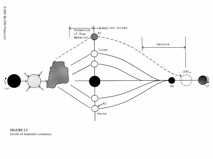
Figure 1.3 shows a schematic of the different levels at which matter canexist. Its original, most condensed
cosmic
state is marked as “O.” Under var-ious forces, it disintegrates and forms local material manifestations, one ofthem being the engineering material. The disintegrated matter, under vari-ous forces, tries to return to the ‘O’ state; perhaps the states “O” and ‘O’ arethe same! The engineering material, at the local level, also starts from agiven state (RI) and, under local engineering forces, tends toward the local(FA) state; (FA)
�
is the ultimate nonmeasurable state. This may be treatedanalogously to the seed, which germinates into a tree (a mixture of orderand disorder) and then coalesces into the seed. The “morning star” and“evening star” were thought to be different, but it was found that both arethe planet Venus! Thus, although we deal with the transformed materialstate in the engineering sense, in a philosophical sense, the initial and finalmaterial states are probably the same.
Time present and time past are both perhaps present in time future, andtime future contained in time past.
…
What might have been and whathas been point to one end, which is always present.
T.S. Eliot (
Burnt Norton
)
Perhaps, we can replace
time
by
matter
.
“We know now that we live in a historical universe, one in which, notonly living organisms, but stars and galaxies are born, mature, grow oldand die. There is good reason to believe it to be a universe permeated withlife, in which life arises, given enough time, wherever the conditions existthat make it possible,” said Nobel laureate Wald (4).
Many quantum physicists have related the understanding of matter withcosmological concepts from the Eastern theological and mystical traditions(5–8). The central role of consciousness in the comprehension of matter in theVedic tradition has been found to compare with the conclusions of modernphysical thoughts (8, 9). Erwin Schrödinger (5), one of the pioneers of quan-tum mechanics, believed that the issues of determinism can be understoodessentially through the Vedic concept of unique and all-pervading con-sciousness, which is composed of the consciousness of individual compo-nents of matter. These and other (recent) thoughts make us aware thatscientific and religious (mystical) concepts can essentially be the same; bothcan lead to the understanding of matter as it exists and to the reality (“truth”or “sat”) of the existence.
There is only one consciousness, and all manifestations (matter, livingand nonliving) are that (or parts) of that consciousness. Goswami et al. (8)propose the concept of monistic idealism. Here the dualism of mind andmatter does not exist, but they interact and exchange energy, and con-sciousness is considered to be the basic element of reality. This conceptstates that everything including matter exists in and is manipulated fromconsciousness.
Ch-01 Page 5 Monday, November 13, 2000 5:58 PM
© 2001 B
y CR
C P
ress LLC
FIGURE 1.3
Levels of material’s existence.
Ch-01 Page 6 M
onday, Novem
ber 13, 2000 5:58 PM
© 2001 B
y CR
C P
ress LLC

© 2001 By CRC Press LLC
The well-known Indian scientist, J.C. Bose, found that apparently nonlivingmatter (e.g., plants) possesses properties similar to those in animate matter;he developed the Crescograph to measure them experimentally. His findingsimplied that the boundary between the animate and inanimate vanishes, andpoints of contact emerge between the domains of the living and nonliving.
The manifested matter, which derives from the same origin (premordial mat-ter), whether animate or living, inanimate, metal, plant, and animal, may followthe same universal law of causality involving action and reaction. They all mayexhibit essentially similar phenomena of stress, degradation and fatigue(depression), growth or stiffening (exhilaration), and potential for recovery, aswell as permanent unresponsiveness (failure or death at the local level).
Response of the matter, then, is governed by metaphysical laws, whichinclude the mechanistic laws as a subset. Our modelling is based on the mech-anistic laws and does not include what exists between the mechanistic andthe metaphysical, which is most probably governed by the nonidentifiableand inconceivable property of consciousness that resides in the life force(
prana
,
chi
) between the material particles. It is this property that may be acause of the
interaction
between (clusters of) material particles, which at themechanistic level can be considered to be defined through the
characteristicdimension
. Hence, a model to describe the response of the material is requiredto include the characteristic dimension. The DSC includes this propertyimplicitly in its formulation.
The motion of particles in any physical system leads to a transition fromone state at an instant of time to the next state at the next instant of time.When the next state occurs, the existence of the previous state ceases, but itsinfluence does not. There is always a gap, however small, between the twostates. In mechanics, we try to characterize the physical motion from onestate to the next by treating the material particle as an inert entity. However,the influence of the gap (which is not known) and of what is contained in itcan be profound on the motion from one state to the next; “the things that wesee are temporal, but things that are unseen are eternal” (II Corinthians 4:18).It is this influence that may govern the capability of the physical entities toself-adjust or self-organize under the influence of external forces. The issuethen is the transformation from one material state to the next. Indeed, thelaws of physics and mechanics can be invoked to characterize the transfor-mation as it refers to the skeleton made of inert particles. However, the mate-rial does exhibit the attribute of natural self-adjustment to organize such thatit responds to the external forces in the optimum way.
1.2.3 Local and Global States
It is apparent that what we have discussed above refers to “local” materialstates, for “finite” physical systems such as engineering structures. How-ever, in the global or universal sense, similar manifestations occur in whichthe initial
premordial
or
pristine
material is transformed continuously undercosmic forces and approaches in the limit the ultimate state. It is possible
Ch-01 Page 7 Monday, November 13, 2000 5:58 PM

© 2001 By CRC Press LLC
that what happens at the local level is perhaps the reflection of what hap-pens at the global level. Our interest is the local behavior.
1.3 Engineering Materials
Engineering materials are difficult to characterize in their initial natural orartificially manufactured states. Characterization of their behavior under avariety of possible forces—natural, mechanical, and environmental—alsoposes a challenging problem.
Human understanding of the behavior of materials, which are a mixture of“continuous” and “discontinuous” particle systems
at the same time
, involvesmental (human), physical, and mathematical models; the latter are often usedto develop numerical models for solution by the
artificial mind
, which is themodern computer.
1.3.1 Continuous or Discontinuous or Mixture
The long pursuit of the mechanics of engineering materials has grappled withthe notion that the materials’ systems can be treated as
continuous
, such thatparticles or clusters at the level of interest do not separate or do not overlap.A moment’s mental reflection and probing would reveal that particles at anylevel are not continuous as there is always a gap, or void (“shunya” or space),between them. At the same time, there is some known and some unknownand mysterious thread or force or synchronous cohesion that connects the par-ticles. Even if all physical and chemical forces that contribute to this connec-tion are identified and quantified, there “appears” to exist a force beyond allquantifiable forces that remains to be identified and quantified. Some wouldsay that when the complete understanding occurs there would be no furtherneed to characterize materials, and all will become (again) one materialwhole! Also, this makes us aware of the fact that the models we develop tocharacterize the material behavior are only approximations, as they do notcompletely characterize the response of the entire, or
holistic,
system.Thus, the limitation of our understanding of the complex discontinuous system
requires us to treat materials as continuous. The reality appears to be that bothcontinuous and discontinuous exist simultaneously, i.e., a particle at a givenlevel is connected and disconnected to others at the same time. Hence, in ageneral sense, almost all reasonably successful efforts and models, in physicsand mechanics, until now, have involved some sort of superposition or impo-sition of discontinuity on continuity. Then, the available continuum models ortheories are very often enhanced or enriched by models or constraints to sim-ulate discontinuity.
It is with the foregoing appreciation of the limitation of our modelling thatwe will deal with materials that are both continuous and discontinuous at thesame time.
Ch-01 Page 8 Monday, November 13, 2000 5:58 PM

© 2001 By CRC Press LLC
1.3.2 Transformation and Self-Adjustment
The local and global transformation of the material world, in its physical man-ifestation and in its “hidden” metaphysical attributes, interests us. One maysay that it is this transformation that makes motion or “life” and that makesour endeavors necessary and possible. If we restricted ourselves to the phys-ical world and the transformation did not occur, there would be no problemto solve. Under the external influences, however, the present state of the mate-rial changes, and the material modifies its present state to a new state underthe given influences. It is the transformation from the present to the new state,so as to define the new state, a process that involves motion or movement ofparticles, that is the objective of mechanics of materials.
How and why the transformation occurs are important issues in under-standing the transformation. The particles constituting the material “yield,”or move, so as to resist optimally the external influences, which, in our case,are the mechanical and environmental forces. The particles may cometogether, move away from each other, rotate by themselves, and
�
or slip withrespect to each other. These motions result in the changes in the physicalstate of the material, which is usually manifested as changes in the shape,size, and orientation of the material body that is comprised of the particles.Hence, in order to define the new state of the body, it becomes necessary toevaluate the motions under the loads the body is carrying so that we can saywith certainty that the engineering body would not “fail,” i.e., break apart inthe local sense, and move away unacceptably.
The Oriental (Indian and Chinese) and early Western (Greek) thinkersbelieved that all matter is “living” (6, 7, 10, 11). The idea that a material respondsonly mechanistically through physical response (motions), which is the founda-tion of modern science, arose when the attribute of life or consciousness waseliminated from the part of the material world, which we defined as “dead” or“nonliving.” This is tragic, since an appreciation of “life force” in materials cannot only help in developing enhanced understanding, but can also lead to thehumanization of technology (12).
If the quality of self-adjustment is accepted, the pursuit of the understand-ing of material behavior may open new vistas. At this time, the issue can becontroversial—particularly in the treatment of mechanics of materials in thetechnological context—but its appreciation may be interesting to those whowould like to read further, think it over, analyze, speculate, and accept orreject it.
1.3.3 Levels of Understanding
Engineering materials involving a mixture of continuous and discontinuousparts represent complex and nonlinear systems. Hence, it is usually not pos-sible to treat their behavior as simple linear responses or to treat them as adirect accumulation of responses of individual particles or a cluster of parti-cles; from now on, both will be referred to as
particles
. This is partly becausesuch an accumulation would lose at least a part of the influence due to the
Ch-01 Page 9 Monday, November 13, 2000 5:58 PM

© 2001 By CRC Press LLC
interconnectedness of the particles. For instance, consider the motion of ahandball that bounces repeatedly on the walls of the court. If the motion ofthe ball were a collection of linear events, it would theoretically be possibleto predict its location at any time. However, as the ball itself is not ideallysmooth and the walls and floor of the court are rough and undulated, themotion of the ball is nonlinear, and it is almost impossible to predict its
exact
location with time. In this connection, it is interesting to paraphrase Bak andChen (13): it is not realistic to predict the behavior of a large interactive sys-tem by studying its elements and microscopic mechanisms separately,because the response of such a system is not proportional to the disturbances.This implies that the theories for modelling the material behavior based onthe micromechanics approach may not provide a rational means of represent-ing the behavior of the
complex interacting
systems such as engineering mate-rials. Indeed, like many available models, they do provide an approximatesimulation of the behavior. In the micromechanics models, the behavior ofparticles is first defined at the local particle (micro-) level, in terms of, say, itsshear and normal responses. Then the local or microlevel (constitutive)responses are accumulated to obtain the overall or global response. And veryoften, the constitutive response at the microlevel is defined based on tests onfinite-sized specimens. This appears to be a contradiction.
It would seem appropriate that approaches to define the behavior at themacro- or global level based on particle
mechanisms
that allow for interact-ing phenomena at the local or microlevel and changes in the microstruc-ture may lead to more consistent theories for the nonlinear and complexmaterial systems. The DSC presented in this book is one such approach.The self-organized criticality (SOC) concept (13; Appendix I) to define crit-ical or threshold states during microstructural changes is another approachthat provides models for instability and collapse by considering the inter-acting mechanisms rather than particle-level descriptions. As will be dis-cussed later, the DSC provides for the instability, or collapse, as well asthe precollapse response. Hence, it is considered to be general and uni-fied; Appendix I presents a review of and comparison between the DSCand SOC.
1.3.4 The Role of Material Models in Engineering
Understanding the behavior of matter or materials is a continuing humanpursuit involving qualitative and quantitative considerations. The former isbased essentially on intuitive and empirical evidence or experience. Intui-tive understanding is often based on philosophical and metaphysical inter-pretations, whereas the empirical comprehension is based on empiricalevidence that leads to simplified models. Although they can describe theresponse of the material approximately, models based strictly on empiricaldata may not lead to the fundamental approaches often required for thebasic description of physical and engineering systems.
Ch-01 Page 10 Monday, November 13, 2000 5:58 PM
© 2001 By CRC Press LLC
Hence, it becomes necessary to develop models based on a combinationof mathematics and mechanics, and empirical data, to lead to the calculation ofpractical quantities such as deformations and stresses required for analysisand design. This approach leads to mathematical expressions or models thatconnect the response of materials to the (external) mechanical and environ-mental forces. This connection depends on the behavior of materials, theirconstitution, and their characteristics. We call these expressions
constitutivelaws
,
constitutive models
, or
constitutive equations
. Constitutive laws play a vitalrole in the prediction of the response of engineering systems. Their develop-ment requires consideration of physical laws as well as observations of theirbehavior under laboratory and/or field conditions that simulate the factorssuch as loading, geometry, and constitution of materials.
The behavior of engineering systems composed of materials as influencedby the foregoing factors is usually complex. Hence, it is often not possible toemploy solution procedures such as those based on closed-form mathemati-cal solutions of differential equations with simplifying assumptions regard-ing the material properties, geometry, etc. Hence, modern computationalmethods are often used to solve such nonlinear problems. As a consequence,it becomes necessary to introduce the advanced and realistic constitutivemodels in such computational procedures as the finite-element, boundary-element, and finite difference methods. Here, the complexities and nonlinearityrequire special attention toward the robustness and reliability of the com-puter predictions.
1.4 Disturbed State Concept
This book deals with the disturbed state concept (DSC), which is based on thewell-recognized idea that a mixture’s response can be expressed in terms ofthe responses of its interacting components. In the case of the same engi-neering material, the components are considered to be material parts in therelatively intact (RI) or “continuum” state and the fully adjusted (FA)state, which is the consequence of the self-adjustment of the material’smicrostructure and can involve decay (damage) or growth (healing).Before the load is applied, the material can be in the continuum state with-out any disturbance such as anisotropy, microcracking, and flaws; in otherwords, initially the disturbance is zero. Alternatively, the material mayhave initial anisotropy, microcracking, and flaws; in that case, there is non-zero initial disturbance.
As loading progresses, the material transforms progressively from the RIstate to the FA state through a process of internal
self-adjustment
of its micro-structure. This process can involve local (microlevel) unstable or disorderedmotions of particles tending toward the FA state, in which there may occur“isotropic” particle orientation. A special case of such an orientation is the
Ch-01 Page 11 Monday, November 13, 2000 5:58 PM
© 2001 By CRC Press LLC
development of distinct cracks, which can be considered to be the
null
isotro-pic state, as in the case of the classical continuum damage models. It is recog-nized that the material experiences growth and coalescence of microcracks,which may lead to distinct cracks. However, the material may often “fail”before the formation of distinct cracks. Hence, the assumption that the FA isthe cracked state and acts like a “void” may not be realistic because as thematerial parts in the FA state are surrounded by the RI material, they possessa certain stiffness and strength. As a result, the RI and FA parts involve
inter-acting mechanisms
that contribute to the response of the mixture. The FA stateis asymptotic and cannot be measured in the laboratory because, before it isreached, the material ‘‘fails’’ in the engineering sense. The FA state is usuallydefined approximately. For example, it can be defined based on the ultimate(asymptotic) disturbance,
D
u
(Fig. 1.2). The asymptotic value (
D
�
1) is notmeasurable when the final FA state is reached.
In the DSC, the disturbance that connects the interacting responses of theRI and FA parts in the same material (or of the components as reference mate-rials) denotes the deviation of the observed response from the responses ofthe reference states (Fig. 1.2). Thus, depending on the material properties,geometry, and loading, it can represent both decay (damage) or growth(healing or stiffening) in the observed response. For instance, in some cases,the microcracks may grow continuously and result in damage, softening, ordegradation of the response, while in other cases, healing (of microcracks)may occur and lead to strengthening or stiffening of the response. Thus, theDSC can allow for the characterization of both the damage and stiffeningresponses.
As the formulation of the DSC involves both the RI (continuum) and FAstates, it provides a systematic
hierarchical
basis for a wide range of models tocharacterize the material behavior. For example, if there is no disturbance, theDSC specializes to continuum models such as elasticity, plasticity, and visco-plasticity. If the material behavior involves microcracking and fracturing,
D
is nonzero and various models such as damage with microcrack interactionare obtained. Because the DSC involves interaction between the responses ofmaterial parts in the reference states, it can allow for nonlocal effects andcharacteristic dimension without external enrichments such as Cosserat andgradient theories.
1.4.1 Disturbance and Damage Models
There is a basic difference between the DSC and the classical continuumdamage approach (14). In the DSC, we start from the idea that the materialunder load can be considered a mixture involving continuous interactionbetween its components. Depending on the mechanical and environmental(thermal, fluid, chemical, etc.) loading, the material mixture can undergodegradation in its strength and stiffness, which leads to the decay or damage-type phenomenon. This is similar to the classical damage approach.
Ch-01 Page 12 Monday, November 13, 2000 5:58 PM

© 2001 By CRC Press LLC
However, the starting point in the damage approach is different; it startsfrom the assumption that a part of the material is damaged or cracked. Theobserved behavior is defined based essentially on that of the remainingcontinuum or undamaged part. Hence, the damaged part involves no inter-action with the continuum part. However, the so-called damaged part mayusually become a finite crack or void
only
near the end or failure, becausein reality the ‘‘damaged’’ part is the result of the continuous coalescence ofmicrocracks and it possesses certain strength. In the DSC, the FA part rep-resents the distributed, coalescent smeared microcracks, with appropriatedeformation and strength characteristics. As a result, the RI and FA partsinteract continuously, which is absent in the classical damage model. Inorder to introduce the microcrack interaction, the damage model requires“external” enrichments such as through kinematics and forces in a (large)number of microcracks, which can add significant complexities. Moreover,as the constitutive behavior of two or more microcracks is not readily meas-urable, inconsistent assumptions are needed to define the behavior. Forinstance, very often the microcrack behavior is defined based on test data onmacro- or finite-sized specimens.
On the other hand, the DSC includes in its formulation the microcrackinteraction through the interacting mechanisms between the RI and FAparts. Also, the definition of the behavior of the material parts in the RI andFA parts relies on the observed (laboratory) behavior of macrolevel orfinite-sized specimens. Thus, the DSC model is rooted in the microstruc-tural consideration but does not require constitutive definition at the parti-cle or microlevel. This is considered a distinct advantage compared to thedamage models with (external) microcracks interaction and the microme-chanical models.
The other major difference between the DSC and damage models is that theforegoing viewpoint in the DSC allows for the possibility of growth or heal-ing, leading to strengthening or stiffening, respectively, of the response of thematerial under mechanical and environmental loading. Such behavior is pos-sible in many situations, including the case when the material undergoingmicrocracking and degradation up to a certain threshold or critical deforma-tion state may heal due to factors such as unloading, chemical reaction, oxi-dation, and locking of microcracks or dislocations. Thus, the DSC includesthe possibility of both decay and growth processes, whereas the damagemodel allows mainly for the degradation or softening response.
1.4.2 The DSC and Other Models
Comparisons between the DSC and other models such as the continuum anddamage approach, with enrichments like the gradient and Cosserat theories,and the micromechanics approach are presented in other chapters (e.g.,Chapter 12). Appendix I presents a review of and comparison between theDSC, critical-state, and SOC concepts.
Ch-01 Page 13 Monday, November 13, 2000 5:58 PM

© 2001 By CRC Press LLC
1.5 Scope
The scope of this book involves the theoretical development, calibration, andvalidation of the DSC and its specialized versions.
1.5.1 Outlines of Chapters
Brief descriptions of this book’s other chapters, including their computa-tional, validation, and mathematical characteristics, follow.
In Chapter 2 we present preliminaries of the DSC, including its unified char-acter, mechanisms of deformation, the derivation of the DSC equations, andspecializations such as composite systems and porous materials. Compari-sons of the DSC with other models, and with the SOC, are also presented;however, details of such comparisons are given in Chapter 12 and Appendix I.
The details of the RI and FA states and the disturbance are presented inChapter 3. Chapter 4 gives details of the incremental DSC constitutive equa-tions, their specializations, and the parameter determination for the distur-bance function and models for the fully adjusted state.
Chapters 5 to 8 discuss various theories—elasticity, plasticity, hierarchicalsingle-surface plasticity, and viscoplasticity—based on continuum mechanicsincluding thermal effects, for characterizing the RI response. They includederivations and examples of DSC in which elasticity, plasticity, and visco-plasticity are used to characterize the RI response. Chapter 7 describes thehierarchical single-surface (HISS) plasticity models commonly used for char-acterizing the RI response. These chapters present examples of a number ofmaterials, including the determination of material parameters from laboratorytests and validation of the constitutive models with respect to the laboratorybehavior for the test data used for finding the parameters and
independent
testsnot used to find the parameters.
Chapter 9 presents the DSC for saturated and partially saturated materials, inwhich formulations and validation of the DSC for saturated and partially satu-rated materials including instability (liquefaction) are described. Chapter 10deals with characterizing the behavior of “structured” materials, such as stiff-ening or healing.
Chapter 11 describes the development of the DSC for interfaces and jointsusing the same mathematical framework as for the “solids.” It includes param-eter determination as well as validation with respect to laboratory tests for anumber of interfaces and joints. Microstructure, localization, threshold tran-sitions, instability and liquefaction, and spurious mesh dependence are dis-cussed in Chapter 12.
Chapter 13 gives details of the implementation of the DSC models in com-puter (finite-element) procedures. It includes mathematical characteristics ofthe DSC, predictions and validations of the observed behavior of a numberof practical boundary-value problems, and descriptions of computer codes.Finally, conclusions and future trends are presented in Chapter 14.
Ch-01 Page 14 Monday, November 13, 2000 5:58 PM

© 2001 By CRC Press LLC
Appendix I offers a review of and comparisons among the DSC, critical-state (CS), and SOC concepts. Computer procedures for the determinationand optimization of material parameters, including validations of laboratorytest data, are presented in Appendix II.
References
1. Miller, J.,
The Vision of Cosmic Order in the Vedas,
Routledge & Kegal Palu,London, 1985.
2. Swami Nikhilananda,
The Upanishads,
Harper Torchbooks, New York, 1963.3. Griffiths, R.T.H., The Hymns of the Rigveda, Motilal Banarasidas, New Delhi,
India, 1973.4. Wald, G., “The Cosmology of Life and Mind,” in Synthesis of Science and Religion,
Singh, T.D. and Gomatam, R. (Editors), The Bhaktivedanta Institute, SanFrancisco, CA, 1987.
5. Schrödinger, E., What Is Life?, MacMillan Publ. Co., New York, 1965.6. Capra, F., The Tao of Physics, Shambhala, Berkeley, CA, 1976.7. Zukav, G., The Dancing Wu Li Masters: An Overview of the New Physics, William
Morrow and Co., New York, 1979.8. Goswami, A., Reed, R.E., and Goswami, M., The Self-Aware Universe: How
Consciousness Creates the Material World, Penguin Putnam, Inc., New York, 1995.9. Fuerstein, G., Kak, S., and Frawley, D., In Search of the Cradle of Civilization,
Quest Books, Wheaton, IL, 1995.10. Swami Nikhilananda, The Upanishads, Harper Torchbooks, New York, 1963.11. Max Müller, F. (Translator), The Upanishads, Oxford University Press, Oxford,
1884.12. Prigogine, I. and Stengers, I., Order Out of Chaos: Man’s New Dialogue with
Nature, Bantam Books, New York, 1984.13. Bak, P. and Chen, K., “Self-organized Criticality,” Scientific American, January
1991.14. Kachanov, L.M., Introduction to Continuum Damage Mechanics, Martinus Nijhoff
Publishers, Dordrecht, The Netherlands, 1986.
Ch-01 Page 15 Monday, November 13, 2000 5:58 PM

© 2001 By CRC Press LLC
2
The Disturbed State Concept: Preliminaries
CONTENTS
2.1 Introduction2.1.1 Engineering Behavior
2.2 Mechanism2.2.1 Fully Adjusted State2.2.2 Additional Considerations2.2.3 Characteristic Dimension
2.3 Observed Behavior2.4 The Formulation of the Disturbed State Concept2.5 Incremental Equations
2.5.1 Relative Intact State2.5.2 Fully Adjusted State2.5.3 Effective or Net Stress
2.6 Alternative Formulations of the DSC2.6.1 Material Element Composed of Two Materials
2.7 The Multicomponent DSC System 2.8 DSC for Porous Saturated Media
2.8.1 DSC Equations2.8.2 Disturbance2.8.3 Terzaghi’s Effective Stress Concep2.8.4 Example and Analysis2.8.5 Comments
2.9 Bonded Materials2.9.1 Approach 12.9.2 Approach 22.9.3 Approach 32.9.4 Approach 42.9.5 Porous Saturated Bonded Materials2.9.6 Structured Materials
2.10 Characteristics of the DSC2.10.1 Comparisons and Comments2.10.2 Self-Organized Criticality
2.11 Hierarchical Framework of the DSC
ch-02 Page 17 Monday, November 13, 2000 5:55 PM

© 2001 By CRC Press LLC
Matter is continuous and discontinuous, ordered and disordered, finiteand infinite at the same time. Each component has asymptotic attributesthat cannot be defined exactly. They culminate or dissolve in each other,can undergo decay and growth at the same time, and yield the intercon-nected composite that can be defined and understood locally.
2.1 Introduction
A deforming material is considered to be a mixture of “continuous” and “dis-continuous” parts. The latter can involve relative motions between particlesdue to microcracking, slippage, rotations, etc. As a result, the conventionaldefinition of stress (
�
)
�
at a point
given by
(2.1a)
where
P
is the applied load and
A
is the area normal to
P
, does not hold; Fig.2.1(a). The implication of is that the stress is defined at a point. Inother words, all points in the material elements retain their neighborhoodsbefore and during load. As a result, abrupt changes in the stress at neighbor-ing points cannot exist, as no cracks or overlaps are permitted.
Now, consider a material element that contains discontinuities due tomicrocracking and fractures, initial or induced voids or flaws. In this case, thedefinition of stress, Eq. (2.1a), will not hold, as the stress may change—andabruptly—from point to point in the material element. In other words, the so-called local (at a point) relevance of stress loses its meaning when discontinu-ities exist. As a result, it becomes necessary to define a weighted value ofstress, , to represent its
weighted
distribution over the material element:
(2.1b)
where is the weighted
nonlocal
area that includes the effect of discontinuitiesin the “finite” area over which is now evaluated (Fig. 2.1(b)). Such anapproach is consistent with the physical necessity for the stress to includethe effects and attributes of the happenings (deformations) in the neighboring
�PA----
A 0→
�
A 0→
�
�PA----�
A�
�
�
Sign convention: For materials that are loaded mainly in tension, the (normal) stresses are con-sidered to be positive. The compressive (normal) stresses are considered positive for materialloaded mainly in compression.
ch-02 Page 18 Monday, November 13, 2000 5:55 PM

© 2001 By CRC Press LLC
FIGURE 2.1
Definitions of stress.
ch-02 Page 19 Monday, November 13, 2000 5:55 PM

© 2001 By CRC Press LLC
regions. The DSC allows consideration of the nonlocal effects by defining thestress (Chapters 3 and 12) in a weighted sense, such that the effect of the dis-turbance (microcracking, etc.) is included in the observed or actual stress.
As introduced in the previous chapter, the
disturbed state concept
(DSC) isbased on the basic physical principle that the behavior exhibited throughthe interacting mechanisms of components in a mixture can be expressedin terms of the responses of the components connected through a couplingfunction, called the
disturbance function
(
D
). In the case of the mechanicalresponse of deforming engineering materials, the components are consid-ered to be reference material states. For the element of the
same
material,the reference material states are considered to be its (initial) continuum orrelative intact (RI) state, and the fully adjusted (FA) state that results fromthe transformation of the material in the RI state due to factors such as par-ticle (relative) motions and microcracking. We first consider the DSC for thecase of deformations in the
same
material. Then we shall consider the DSCfor deforming a material element composed of more than one (different)material.
Analogies for Reference States
. If a solid is heated at a certain tempera-ture, it melts or liquefies. The solid and liquid states can then represent tworeference states. If the liquid is heated further, it becomes a gas. Then the liq-uid and gas states can represent the reference states. If a cube of ice melts towater, the ice and water states can be treated as the reference states.
A schematic of the underlying idea in the DSC is shown in Fig. 2.1(c). Thematerial possesses asymptotic (relative) intact and fully adjusted states (Fig. 2.2).The
absolute intact
state may be considered to be the condition of the material, say,at the
theoretical maximum density
(TMD). However, as explained in Chapter 1, thematerial can exist at other densities, which can be adopted as RI states. Selectionof the RI state depends on the characteristics of the material and available testdata. For instance, the linear elastic response of a continuum without micro-cracks can define the RI (e) response with respect to the nonlinear elastic(observed, denoted by
a
) response affected by microcracking; see Fig. 2.2(a). Theelastoplastic (ep) behavior without friction can define the RI response withrespect to the elastoplastic behavior with friction; see Fig. 2.2(b). The elastoplasticresponse can be adopted as the RI response with respect to the behavior affectedby microcracks and softening; see Fig. 2.2(c). Figure 2.2(d) shows a schematic ofsoftening and stiffening responses in which the RI response is characterized aselastoplastic.
The asymptotic FA state, (FA)
∞
, is the final condition to which the materialapproaches under external loading [Fig. 2.2(c)]. The behavior of materials atthe final state is not measurable in the laboratory but may be defined as theasymptotic value that can be identified approximately. Such a state used inthe modelling is considered quasi-FA ( ), which, for convenience, isreferred to simply as the FA state.
The behavior of a material differs when affected by factors such as initialpressure, density, and temperature. Also, there can be more than one RI andFA states. However, the response of the material parts in the RI and FA states
FAFA
ch-02 Page 20 Monday, November 13, 2000 5:55 PM

© 2001 By CRC Press LLC
can be expressed in terms of the foregoing factors, which leads to an inte-grated (DSC) model. This aspect is discussed later in the chapter.
2.1.1 Engineering Behavior
Figure 2.3(a) and (b) show schematics of the response of a material elementunder the shear stress , the second invariant of the deviatoric stresstensor
S
ij
, and
J
1
, the first invariant of the total stress tensor,
�
ij
, which isrelated to the mean pressure,
p
, as
p
�
J
1
�
3. It is assumed that the materialis initially isotropic and remains isotropic during deformation.
Pure shear stress (with
J
1
�
0) will cause continuing shear deformations thatwill lead to an observed engineering “failure” condition (marked 1 in Fig. 2.3(a))that can be measured in the laboratory. It can be identified as the peak stress orasymptotic or ultimate stress with respect to the behavior in the final range ofthe stress–strain behavior. Upon further loading, the material may disintegrate
FIGURE 2.2
RI(i), observed (a), and FA (c) responses.
J2D
ch-02 Page 21 Monday, November 13, 2000 5:55 PM

© 2001 By CRC Press LLC
fully and separate into individual particles (1
�
); this response cannot be meas-ured. Under pure (compressive) mean pressure (
�
0), the material com-pacts and strengthens continuously and will reach the measurable state (2) andnonmeasurable state (2
�
).A combination of and
J
1
leads to measurable ultimate or failurestates defined by the envelope shown in Fig. 2.3(a). The nonmeasurable orasymptotic states may lead to the disintegration of the element under dif-ferent combinations of and
J
1
.Figure 2.3(b) depicts vs. response under pure shear stress (
J
1
�
0); here is the second invariant of the deviatoric strain tensor,
E
ij
. Forpure mean pressure , the volume will change (decrease) continu-ously. With both and
J
1
, the stress–strain response affected by both the
FIGURE 2.3
Material states during loading.
J2DJ2D
J2D
J2D
J2D I2D
I2D
J2D � 0( )J2D
ch-02 Page 22 Monday, November 13, 2000 5:55 PM

© 2001 By CRC Press LLC
shear stress and mean pressure will result. Then the RI response can be char-acterized by using elastic, elastoplastic, or another suitable model (Fig. 2.2).The FA response can be defined at the critical state (c) the material approachesunder given mean pressure.
Historical Note.
The basic idea underlying the DSC derives from themodel for overconsolidated geologic materials proposed in 1974 by Desai (1)in the context of the solution of the problem of slope stability. It was postulatedthat the behavior of overconsolidated (OC) soil can be decomposed into that ofthe normally consolidated (NC) and that due to the influence of overconsol-idation that entails microcracking and shear planes; see Fig. 2.4(a). Then theobserved softening response was expressed in terms of the behavior under theNC state and the effect of overconsolidation. The observed response (stiffness)was then expressed in terms of the stiffness of the two parts. Desai (2) proposedthe concept of the residual flow procedure (RFP) for the solution of free surfaceflow (seepage) in porous media (3, 4); a review is presented by Bruch (5). Herethe response was decomposed into two reference states: the fully saturatedwith the permeability coefficient,
k
s
, and the “residual” response given by thedifference between the saturated and unsaturated (or partially saturated) con-ditions due to the difference in permeability coefficients,
k
s
�
k
us
(Fig. 2.4(b)).Thus, the two reference states were given by the saturated state and the asymp-totic unsaturated state at very high negative pressures (
p
).The DSC presented in this book can be considered as a generalization of the
foregoing two developments in stress analysis and flow through porousmedia.
2.2 Mechanism
An initially intact material, without any flaws, cracks, or discontinuities, willtransform continuously with loading, unloading, and reloading, which is oftenreferred to collectively as loading, from the RI state to the FA state [Fig. 2.1(c)].If the material before the loading contains initial flaws, cracks, and
�
or disconti-nuities (or disturbance), the resulting initial disturbance will influence the sub-sequent behavior. As the deformation progresses, the extent of the materialparts, which may be distributed randomly over the material element depend-ing on factors such as initial conditions and loading, the FA parts can growor decrease, i.e., lead to degradation or stiffening, respectively [Fig. 2.2(d)]. Inthe case of the continuous growth of the FA state, the material part in the RIstate decreases continuously, during which the microstructural changes caninvolve the annihilation of particle bonds, leading to a decay process. In thelimit, if it is possible to continue the load, the entire material will approach the(FA)
∞
state, in which the material particle may break and separate completely,and then the disturbance approaches the value of unity. As this state is asymp-totic, it is not realized in practice—in the field or in the laboratory—because the
ch-02 Page 23 Monday, November 13, 2000 5:55 PM

© 2001 By CRC Press LLC
material “fails,” in the engineering sense, in terms of allowable deformationand
�
or load before the (FA)
∞
state can be reached. Hence, from practical consid-eration, it often becomes necessary to identify and use approximately the state when the material enters the ultimate residual state for given initial con-ditions in the engineering sense when the disturbance
�
D
u
(
�
1.0). This stateis used as the FA state from a practical viewpoint (Fig. 2.2).
In the DSC, the microstructural changes may be such that the material maystiffen due to strengthening of the interparticle bonds [Fig. 2.2(d)]. This mayoccur due to factors such as predominant hydrostatic stresses that lead to
FIGURE 2.4
Disturbance in stiff or structured soil, and flow through a partially saturated medium (1–3).
FA
ch-02 Page 24 Monday, November 13, 2000 5:55 PM

© 2001 By CRC Press LLC
increasing density, the structured nature of material, chemical and thermaleffects that lead to increased interparticle bonding and unloading, or restperiods (Chapter 10).
The RI state is often simulated by using such continuum theories as elastic-ity, plasticity, and viscoplasticity for which well-established formulations areavailable. These are discussed subsequently in this chapter and in Chapters5 to 8. Here, we first discuss some aspects of the FA state.
2.2.1 Fully Adjusted State
For engineering materials, the final state at “infinite” or very high loading(Fig. 2.2) may result in a totally disintegrated state in which the separatedmaterial particles tend to configure into a “specific” volume. Such a (‘’loose’’)material may not have any strength at all unless it is confined. The final dis-integrated material state may be considered analogous to the idea of treatingthe cracked or damaged material part as a “void,” as it is assumed in the clas-sical damage mechanics approach (6, 7). One of the main differences betweenthe DSC and the damage concept can be stated here. In the DSC, it is consid-ered that the FA material, in the range of engineering interest,
does
possesscertain deformation and strength properties. This is partly because the FAmaterial parts are confined or surrounded by the material parts in the RI state[Fig. 2.1(c)]. Furthermore, in contrast to the damage concept, in which thedamaged parts grow continuously, resulting in the continuous loss ofstrength, in the DSC, the material can also gain strength or stiffen duringloading. In other words, under certain loadings and physical conditions, theFA state can entail strengthening. Then, disturbance will be “negative” orhave a value greater than unity, indicating strengthening or a growth process.Thus, the DSC allows for the characterization of both degradation (or dam-age or decay) and stiffening (or healing) in material responses.
The idea of the critical state (CS) in soil mechanics has a connotation similarto the FA state. The material
approaches
the critical state at which there is nofurther change in volume, i.e., the material assumes an invariant (specific) vol-ume, void ratio, or density under the constant shear stress reached up to thatstate and given initial mean pressure (8, 9). In practice, however, e.g., in thelaboratory, it is usually not possible to measure and identify the
exact
criticalstate. It is asymptotic, like the FA state. For engineering purposes, we identifyand can often adopt the CS as the FA state when the measured volume changeis
approximately
zero in the ultimate range of loading. Indeed, there may beinstantaneous states of zero volume changes like the point of transition fromcompactive to dilative volume change in granular materials, where one canidentify the point almost exactly; however, the FA state is considered to occurin the ultimate range. To summarize, the definition of material response at theFA state must be approximate because the measurement system would ceaseto operate when the material specimen “collapsed” from an engineering anda practical viewpoint.
ch-02 Page 25 Monday, November 13, 2000 5:55 PM

© 2001 By CRC Press LLC
As a further explanation, let us consider two lumps of a material with dif-ferent initial volumes, and with irregular shapes, as in Fig. 2.5. The irregular-ities or nonsymmetries of the two lumps are the lumps’ initial attributes. Now,let us mold both specimens by applying external pressure to make them “ide-ally” spherical. After the levels of molding efforts have been increased, bothlumps will
tend
toward spherical shapes with different specific, critical, orfully adjusted volumes. It is apparent that it will be (humanly) impossible toachieve the perfect or absolute spherical shapes, with no attributes or irregu-larities or biases. Hence, we must accept approximate spherical shapes withvolumes and at certain levels of effort (loading) to represent the FA stateand use them in our modelling pursuit (Fig. 2.6(a)).
Let us consider the volume of the solid particles as they merge together,when all the particles’ attributes have been annihilated, and the volume, ,at the FA state is approached. The schematic plots of
V
�
for the two lumpsare shown in Fig. 2.6(a). The volume of both approach unity, while and
are the quasi-volumes in the FA state. It is useful to note that the volume (at the FA state) is a unique characteristic for a given set of physical char-
acteristics such as initial density, particle fabric, shape and size, and loading,and can represent the characteristic dimension.
FIGURE 2.5
Molding of clay lumps.
FIGURE 2.6
Behavior of clay lumps.
V1 V2
Vc
Vc
V1
V2
Vc
ch-02 Page 26 Monday, November 13, 2000 5:55 PM

© 2001 By CRC Press LLC
The behavior of an engineering material (specimen) can be understoodsimilarly. The material has initial attributes, like the nonsymmetries causedby anisotropy, flaws, and defects. Now, consider that such a material is sub-jected to increasing hydrostatic or isotropic load (pressure) [Fig. 2.6(b)]. Asthe pressure, like the molding effort for the lumps, is applied, the nonsymme-tries or biases will be annihilated and the material will
tend
toward a “con-densed” (volume of solids) symmetrical or isotropic state with no attributesof anisotropy. The limiting isotropic state, when the nonsymmetry or anisot-ropy (
a
n
), in Fig. 2.6(b), is destroyed completely, will be impossible to achievein practice and in the laboratory. However, approximate states canbe identified, for all practical purposes, to represent the isotropic state, whichcan represent the FA state. As is indicated in Fig. 2.6(b), the material with ini-tial attributes such as anisotropy, flaws, and different particle sizes will tendtoward the isotropic state at different levels of load and effort. Each can haveits own or approximate FA state, which can be adopted as the asymptote toeach response. Indeed, the final asymptotic state is the perfect isotropic state,i.e., A
1
A2 A3 ... A, where A denotes the final FA state.
2.2.2 Additional Considerations
The disturbance, D, is expressed as the ratio of the material volume, , inthe FA state to the total volume, V, of the material element. Hence, for directevaluation of D, one must evaluate the material parts in the FA states duringdeformation. Advanced nondestructive techniques based on X-ray comput-erized tomography and acoustic measurements are being developed, andthey can be used to identify the FA states involving evolution of densityclusters. However, they are still not fully available. Hence, it is not possibleto define D based on such physical measurements. Some limited results areavailable, however. Figure 2.7 shows the vertical reconstruction of a cylin-drical specimen (50.8-cm diameter, 609.6-cm height) of a grout materialtested under triaxial loading by using X-ray computerized tomography (10).
FIGURE 2.7The vertical reconstruction of a failed grout specimen under triaxial compression. (FromRef. 10, with permission.)
an1, an2( )
→ → → →
Vc
ch-02 Page 27 Monday, November 13, 2000 5:55 PM
© 2001 By CRC Press LLC
The measurements were obtained at different stages of loading; Fig. 2.7shows results near (before) the peak stress. The dark regions representmaterial parts that have approached the critical density and can be treatedas being at the FA state. The dark zones were integrated to obtain the vol-ume at the FA state. The ratio D � was about 0.17, which comparedwell with the average values of D at that stage of deformation for similarmaterials (11).
In lieu of direct measurements of the disturbance , it becomes necessary todefine disturbance in terms of internal variables such as accumulated plastic(irreversible) strains and (dissipated) mechanical energy under thermomechani-cal and other loadings. Such internal variables reflect the microstructuralchanges that cause disturbance (damage and�or strengthening). Disturbance canalso be related to observed laboratory response in terms of such measured quan-tities as stresses, volume or void ratio change, porosity change, effective stress(pore fluid pressure), saturation degree, and nondestructive properties such as P-and S-wave velocities (11–14). The use of these phenomenological approachespermits the determination of parameters in the expressions for disturbance;details are given in Chapter 3 and other chapters.
In defining the disturbance (damage or strengthening) in a deformingmaterial, we will be able to take advantage of the similarity between decayand/or growth in natural systems. For example, the mechanism and trend ofgrowth or decay of a living organism can be considered to be similar tostrengthening or decay in a deforming material. As a result, mathematicalfunctions that express decay and growth can be adopted to describe damageand strengthening.
Consider a collection of granular (spherical) material particles, as shown inFig. 2.8. The initial microstructure involves air spaces and contacts, whosemagnitudes will affect the density. The contacts contribute to the deformationand strength properties through interparticle cohesion and friction. Duringdeformation under compressive pressure accompanied by shear stress, theparticles’ contacts can deform, slip, rotate, and break. Furthermore, the parti-cles can move in the air spaces, leading to the change in density.
An initially loose material will experience continuing compaction and anincrease in the density or a decrease in the volume or void ratio, e (volume ofvoids�volume of solids). In general, the material will exhibit a nonlinear andcontinuously hardening response, as seen in Fig. 2.9(a). An initially densematerial first compacts as the particles move in the voids, and then experi-ences an increase in the volume or void ratio or a decrease in the density (Fig.2.9(b)). The latter is called dilation, which is caused predominantly by theupward sliding of the particles.
Depending on the initial nature of the microstructure (distribution of voids,etc.), density clusters can form at different locations, which may tend to the crit-ical invariant density or void ratio (see Fig. 2.8). Such an asymptotic state canrepresent the FA state. As the loading progresses, a greater number of FA statezones develops; in the limit the entire material tends toward the fully adjustedstate.
Vc Vc�V
Vc( )
ch-02 Page 28 Monday, November 13, 2000 5:55 PM

© 2001 By CRC Press LLC
In the case of the initially dense material, behavior similar to that for the loosematerial may continue until the transition from compaction to dilation accom-panied by microcracking or breakage of particle bonds. This process will con-tinue and grow near and after the peak and in the degradation or softeningregime. Increased levels of microcracking, slippage, and rotation of particleswill occur in the softening regime (Fig. 2.9), with locally unstable changes in themicrostructure. Then the microstructure may experience an intense instability,which can be identified by the critical disturbance (Dc) at the initiation of theresidual state, leading to the asymptotic FA state at which there will be nochange in volume or density.
It is possible that during deformation, factors such as chemical reactions,increased compaction, or locking of particle contacts or dislocations can causean increase in the stiffness and strength of the particle bonds. In that case, after
FIGURE 2.8Particle motions, degradation or softening, and healing.
ch-02 Page 29 Monday, November 13, 2000 5:55 PM

© 2001 By CRC Press LLC
a threshold value of deformation or strain ( ), [Fig. 2.9(a)] is reached, the mate-rial may stiffen or heal; this can lead to decreased disturbance. The pore-collapsemechanism in porous rocks, the drained post-liquefaction behavior of saturatedsands, and the locking of dislocations in silicon with oxygen impurity representexamples of such softening and stiffening behavior (Chapter 10).
Figure 2.10 shows the behavior of a porous chalk under hydrostatic loading(15). Here, a cylindrical specimen of the chalk is subjected to confining orhydrostatic stress, and the resulting volumetric strains � (�ii) are measured[Fig. 2.10(a)]. The acoustic P- and S-wave velocities are also measured duringdeformation; see Fig. 2.10(b) and (c).
The initial response of the material is essentially linear elastic (E) with adecrease in the volume; a positive volume indicates a reduction in volume.During this phase, some of the open spaces, initial microcracks, and particlecontacts are closed (15); as a result, the acoustic velocities increase. After about
FIGURE 2.9Schematic of behavior of loose and dense materials.
�1
ch-02 Page 30 Monday, November 13, 2000 5:55 PM

© 2001 By CRC Press LLC
1.0% of the volumetric strain, the particle bonds are broken and the contactcohesion is reduced or lost. As a result, the P- and S-wave velocities decreaseduring this phase, when the collapse of pores occurs (PC). After critical � �6.0%, the material exhibits stiffening (or healing). During this consolidationphase, the acoustic velocities increase as a result of the reestablishment of theparticle contact and bonds.
It can be said that the disturbance will be essentially zero during the initialphase, will increase during the pore-collapse phase, and then will decreaseduring the stiffening phase. Details of the formulation of the DSC for thisbehavior are given in Chapter 10.
FIGURE 2.10Stress–strain, compression, and shear wave responses under hydrostatic compression ofEkofisk Chalk (15).
ch-02 Page 31 Monday, November 13, 2000 5:55 PM

© 2001 By CRC Press LLC
2.2.3 Characteristic Dimension
It is appropriate to mention that factors such as the initial mean pressure, thedensity or void ratio, and the fabric, geometry, and size of particles affect thezone of influence around a point in a material element. The zone of influence isconsidered to be related to the internal or characteristic dimension. In the DSC,the invariant mass or volume which many materials approach duringdeformation can provide an important measure for the characteristic dimen-sion. These aspects are discussed later, e.g., in Chapter 12.
2.3 Observed Behavior
The deforming material is considered a mixture of the two interacting materialparts in the RI and FA states. The RI and FA states are termed as referencestates. Then the observed or actual response of the material is expressed interms of the responses of material parts in the reference states. The distur-bance, D, denotes the deviation of the observed response from those of thereference states. Figure 2.11 shows a symbolic and schematic representationof disturbance in the DSC. The observed or average response (denoted by a)is then expressed in terms of the RI response (denoted by i) and the FAresponse (denoted by c) by using the disturbance function, D, as an interpo-lation and coupling mechanism. The behavior of the RI and FA materials, aswell as the disturbance function, needs to be defined from laboratory tests.
2.4 The Formulation of the Disturbed State Concept
Let us first consider the case of a (dry) material element (Fig. 2.12). Based onthe equilibrium of forces on the material element, composed of the clusters ofparticles in the RI and FA parts, where � observed or average force, �force in the fully adjusted (FA) part, and � force in the relative intact (RI)part, we have
(2.2)
Division of both sides by the total area, A (assuming thickness to be unity)leads to
(2.3a)
Vc( )
Fa Fc
Fi
Fa Fi Fc�
Fa
A----- Fi
Ai----- Ai
A----- Fc
Ac------ Ac
A------���
ch-02 Page 32 Monday, November 13, 2000 5:55 PM

© 2001 By CRC Press LLC
where and are areas corresponding to RI and FA, respectively. Therefore,
(2.3b)
where � observed stress, � stress in the relative intact part, and �stress in the FA part.
2.5 Incremental EquationsEquation (2.3b) can be generalized to three dimensions as*
(2.4)
where D is the disturbance function, D � �A, and 1 � D � �A. Here D is
FIGURE 2.11Representations of DSC.
* Both the tensor and matrix notations are used in this text. The latter can provide for convenientimplementation in computer procedures.
Ai Ac
�a
�i Ai
A----- �
c Ac
A------�
�a
�i
�c
�ija 1 D�( )�ij
i D�ijc
�
Ac Ai
ch-02 Page 33 Monday, November 13, 2000 5:55 PM

© 2001 By CRC Press LLC
assumed to be a scalar in a weighted sense, which implies isotropic condition.However, D can be expressed as a tensor, Dijkl; then
(2.5a)
where Iijk� is the unit tensor. It is difficult to use Eq. (2.5a) because it is usually notpossible to conduct, or to have access to, appropriate laboratory tests for definingthe tensor Dijkl. The multiaxial or three-dimensional test with nondestructive(ultrasonic) measurements (12) is one of the possible tests to define Dijkl; this willbe discussed later. As a simplification, the tensor of disturbance can be expressedas
(2.5b)
where Di (i � 1, 2, 3) are disturbance components in the three principal direc-tions, which can be expressed as
(2.5c)
where �ij are the direction cosines and j denotes the (principal) direction.
FIGURE 2.12Schematic of material element and force equilibrium.
�ija Iijk� Dijk��( )�k�
i Dijk�.�k�
c�
D( )D1 0 00 D2 00 0 D2
�
Di �ijAc
A------
j
�
ch-02 Page 34 Monday, November 13, 2000 5:55 PM

© 2001 By CRC Press LLC
Since certain devices, such as multiaxial three- and two-dimensional devices,can allow measurements in the principal directions, it can be relatively easierto define D in Eq. (2.5b) compared to the definition full tensor, Dijkl. For practicalpurposes, it may often be sufficient to treat D as a scalar. A majority of the treat-ment here uses this assumption.
The incremental form for Eq. (2.4) can be derived as
(2.6a)
where d denotes increment, dD is the increment or rate of D, and �ij is thestress tensor. Equation (2.6a) can now be expressed as
(2.6b)
where and are constitutive tensors for the materials in the RI and FAparts, respectively, and is the strain tensor.
2.5.1 Relative Intact State
As stated earlier, the RI behavior can be characterized by using an elasticity orplasticity model with an associative response or any other suitable continuummodel—viscoplastic, thermoviscoplastic, etc. For example, the �0-version inthe hierarchical single-surface (HISS) plasticity concept (Chapter 7) can beused to represent the RI state. In that case, irreversible deformations and cou-pled shear and volumetric responses will be included in the model; however,factors such as nonassociative response (friction), anisotropy, and microcrack-ing (softening) can deviate or disturb the �0-response to lead to the observedbehavior.
Thus, the RI response is relative in the sense that it excludes the effect of fac-tors that deviate the observed behavior from that of the material in the givenRI state. Hence, the choice of the RI state and corresponding constitutivemodel to define it depend on the material response and available test dataunder given initial conditions that enable characterization and calibration ofparameters for the model for the RI material. As discussed in Chapter 1, thefinal (densest) material state can be treated as the intact state. However, usu-ally each stress–strain response can have its own local RI behavior (Fig. 2.13),e.g., i1 for a1, i2 for a2, and so on, because the response is affected by factorssuch as initial conditions, stress, strain, density, pressure, and temperature.When the �0-model is adopted, the RI plasticity response can be expressed interms of these factors so that the entire range of response, expressed throughdifferent curves (Fig. 2.13), is simulated.
In the same manner, if a nonlinear elastic response is adopted for the RIstate, the dependence of elastic parameters such as elastic modulus, E, and
d�ija 1 D�( )d�ij
i Dd�ijc dD d�ij
c�ij
i�( ) �
d�ija 1 D�( )Cijk�
i d�k�i DCijk�
c d�k�c dD �ij
c�ij
i�( ) �
Cijk�i Cijk�
c
�ij
ch-02 Page 35 Monday, November 13, 2000 5:55 PM

© 2001 By CRC Press LLC
Poisson’s ratio, , or shear modulus, G, and bulk modulus, K, will define theRI response for given initial conditions, e.g.,
(2.7a)
(2.7b)
where p0 � initial mean pressure � ( �1 �2 �3)�3. If a single curve is simu-lated, we use the RI modulus corresponding to the given value of p0. How-ever, for the model for simulating the response as affected by p0, the RImodulus can be expressed as a function of p0, e.g.,
(2.7c)
where and n are parameters.
2.5.2 Fully Adjusted State
As the loading progresses, the material parts in the RI state transform contin-uously to the parts in the FA state. Depending on the initial state and inducedconditions caused by stress, flaws, discontinuities, and microcracking, thematerial parts in the FA state can be distributed randomly over the materialelement [Fig. 2.1(c)]. The transformation occurs due to the self-adjustment ofthe material’s microstructure. It may be surmised that the material particles,while undergoing motions such as translation and rotation, would experi-ence instantaneous instability at the local (micro-) level [Fig. 2.1(c)]. However,the measured macro response would appear as the integration of the locallyunstable responses at the microlevel and may not indicate instability in the
FIGURE 2.13RI and observed states.
E E p0( )�
G G p0( )�
E K p0( )n�
K
ch-02 Page 36 Monday, November 13, 2000 5:55 PM

© 2001 By CRC Press LLC
sense of collapse. The collapse would occur in the ultimate stages when theinstabilities become predominant and critical.
In the FA state, which is asymptotic and cannot be reached or measuredin practice (in the laboratory), the material may organize toward the equili-brated or “isotropic” state with maximum entropy. The structure and thecomposition of the material in the FA state are different from that of thematerial in the RI state. At the same time, both the RI and FA material partsare coupled and interconnected, like water bubbles enclosed at randomlocations in a matrix of solid material particles. It is evident that the behav-ior of the mixture of the material element consisting of a skeleton or matrixof solid particles and the bubbles enclosed in it is dependent on the behav-ior of both. As the bubbles are (totally) enclosed and surrounded by thesolid matrix, they are capable of sustaining a part of the applied load. Onlywhen they are broken and are no longer enclosed, that is, they are con-nected to the atmosphere through cracks in the solid matrix, do they ceaseto sustain any applied load.
The material part in the FA state is analogous to the enclosed water bub-bles in the solid matrix. It can sustain a part of the applied load. Only in thefinal fully adjusted state, denoted by (FA)∞ , may the material experiencetotal breakdown and may the FA part not sustain any load. Such a conditionis asymptotic; before it can be reached, the laboratory testing stops, and thematerial has failed. It is the “engineering” state that we can define anduse in our model. It occurs before the ultimate (FA)∞ state, when the mate-rial “fails” for all practical purposes. It should be noted that only the engi-neering FA state can be measured and is adopted to represent the FA stateapproximately.
There are a number of ways in which we can characterize the behavior ofthe material in the FA state:
• as a constrained liquid-solid. Here a possible representation is thecritical state (8, 9, 11, 12), at which the material experiences con-tinuing shear strains under the shear stress ( or �) reached upto that state with given (initial) pressure (J1�3 or p).
• as a constrained liquid. Here we can assume that the material part cancarry hydrostatic stress or mean pressure (J1�3), but no shear stress( ). That is, as soon as the material part reaches the FA state, theshear stress in it drops to zero (11, 12). This simulation is similar tothe yielding response in the case of a perfectly plastic material whenthe FA stress equals the yield stress; see Examples 6-2 and 6-3 inChapter 6.
• as a finite crack or void. This is similar to the assumption in theclassical damage model (6, 7). Here the material part in the FA statecan carry no stress, that is, � J1�3 � 0. Then the applied loadis carried by the material part in the RI state only, and there is nointeraction between the intact and the damaged parts, although the
FA( )
J2D
J2D
J2D
ch-02 Page 37 Monday, November 13, 2000 5:55 PM

© 2001 By CRC Press LLC
overall observed behavior is modified because of the damagedparts. This assumption is considered to be unrealistic.
• In some cases, the FA state can be adopted corresponding to thematerial response at a reference value of a given parameter. Forinstance, in the case of partially saturated materials, the FA statecan be adopted to correspond with the behavior at full saturationor zero suction (Chapter 9).
In Chapter 4 we will present details of various characterizations for thematerial parts in the RI and FA states.
2.5.3 Effective or Net Stress
In the preceding discussion, we assumed that the material is dry (or drained)and the stresses are effective, that is, they are relevant to the skeleton of mate-rial particles. If the material is saturated with a liquid (water) in the pores orpartially saturated with a liquid together with a gas (air) in the pores, the for-mulation requires modifications. Alternative formulations that cover thiscase are given below.
2.6 Alternative Formulations of the DSC
In the foregoing formulation, Eqs. (2.4) and (2.6), we considered an ele-ment of the same material composed of parts in the RI state and the remain-ing parts in the FA state. The latter is assumed to occur from the verybeginning of the loading, and its extent changes (increases) with loading.The material element is composed of clusters of material particles in the RIand FA states [Fig. 2.1(c)]. The force equilibrium considers the effect of theinteracting particles in the RI and FA states on the observed force (Fa). Inother words, the formulation allows for micromechanical response of theclusters of particles in the two reference states. A major advantage of theforegoing approach is that the responses of the material parts in the RI andFA states can be defined based on the observed laboratory behavior of thesame material element (specimen). For instance, the RI behavior can be char-acterized as linear or nonlinear elastic or elastoplastic by using the observedresponse in the early stages of deformation, whereas the FA behavior can bedefined from the response near the ultimate stage.
The DSC can also be formulated for a material element composed of two(or more) materials whose responses can be treated as reference responses.Here the responses of the component materials may be characterized basedon continuum theories such as elasticity and plasticity. Indeed, it is possiblethat the individual responses of the components may exhibit RI and FA states.
ch-02 Page 38 Monday, November 13, 2000 5:55 PM

© 2001 By CRC Press LLC
Figure 2.14(a) shows a schematic of two component materials used as ref-erence states. Their behavior can be characterized as elastic or elastoplastic,leading to the observed behavior that can be elastic or elastoplastic. In Fig.2.14(b), one of the materials can be characterized as elastic or elastoplastic,whereas the other one can involve microcracking, leading to softening withits own RI and FA responses. Figure 2.14(c) shows two materials, each show-ing softening, and involves RI and FA responses. It is also possible that the
FIGURE 2.14Material element composed of two or more component-reference materials.
ch-02 Page 39 Monday, November 13, 2000 5:55 PM

© 2001 By CRC Press LLC
material is fully or partially saturated with a liquid (e.g., water). Note that forthese situations, it would be necessary to have access to the laboratory behav-ior of each of the materials composing the element and also to the behaviorof the composite . In the following, we present examples of formulationsthat allow for the use of individual materials as reference states.
2.6.1 Material Element Composed of Two Materials
Consider the schematic in Fig. 2.14(c). Each of the two reference materialstates exhibits microcracking and softening behavior and involves FA states.The observed behavior of the mixture of the two materials 1 and 2 can beexpressed as
(2.8a)
Here the term for the composite element is expressed in terms of theobserved responses of materials 1 and 2, e.g.,*
(2.8b)
The term denotes a ratio that is analogous to disturbance, and its defini-tion is different from the disturbance in an element of the same material, e.g.,D1 and D2 in Eqs. (2.8c and d) ahead, which are ratios of the volume in the FAstate to the total volume of the element, Eq. (2.4). Equation (2.4) can now beused to represent the observed stress, , for the composite element.
The observed behavior of each of the materials can be written as
(2.8c)
and
(2.8d)
Hence,
(2.9a)
or in generalized form,
(2.9b)
* General and alternative definitions of D are presented in chapter 3.
�a
�a 1 D�( )�1
a D�2a
�
D
D�1
a�
a�
�1a
�2a
�-------------------�
D
�a
�1a 1 D1�( )�1
i D1�1c
�
�2a 1 D2�( )�2
i D2�2c
�
�a 1 D�( ) 1 D1�( )�1
i D1�1c
[ ] D 1 D2�( )�2i D2�2
c[ ]�
�ija 1 D�( ) 1 D1�( )�1ij
i D1�1ijc
[ ] D 1 D2�( )�2iji D2�2ij
c[ ]�
ch-02 Page 40 Monday, November 13, 2000 5:55 PM

© 2001 By CRC Press LLC
The generalized incremental form of Eq. (2.8a) can be written as
(2.9c)
in which the incremental forms for and can be substituted by usingEqs. (2.8c and d). Thus, laboratory responses of both materials and the mixtureare needed to define Eq. (2.9). The other two situations, Fig. 2.14(a) and (b), canbe derived as special cases of Eq. (2.9). For example, for Fig. 2.14(a),
(2.9d)
and for Fig. 2.14(b),
(2.9e)
2.7 The Multicomponent DSC System
A material element can be considered to be composed of more than two ref-erence materials. Consider that there are n component materials in a materialelement as in Fig. 2.15(a). Then equilibrium of forces gives
(2.10a)
and
(2.10b)
(2.10c)
where � … � 1, which for unit width (b) is given by
(2.10d)
Here, simply denotes the ratios of areas and do not have the same mean-ing as the disturbance in the element of the same material.
d�ija 1 D�( )d�1ij
a Dd�2ija dD �2ij
a�2ij
a�( ) �
d�1ija d�2ij
a
�a 1 D�( )�1
a D�2a
�
�a 1 D�( )�1
a D�2a
�
1 D�( )�1a D 1 D2�( )�2
i D2�2c
[ ]=
Fa F1 F2… Fn �
Fa
A-----
F1
A1------
A1
A------
F2
A2------
A2
A------ … Fn An�
An A�----------------- ���
�1D1 �
2D2 … �nDn �
�Di D1 D2 Dn
�Di
A1
A------
A2
A------ … An
A------
A1 A2… An
A------------------------------------------------- 1� � �
Di
ch-02 Page 41 Monday, November 13, 2000 5:55 PM

© 2001 By CRC Press LLC
Now Eq. (2.10c) can be written as
(2.10e)
In Eq. (2.10e), the strains (i � 1, 2,… ,n) can be different in all the compo-nents, and the “disturbances,” (i � 1, 2,… ,n), can be obtained for eachcomponent as the ratios of areas, Ai�A. Useful specializations can be obtainedby making certain assumptions; if it is assumed that b � 1, can beexpressed in terms of thickness ti (i � 1, 2,… ,n) of each component. Then
(2.11a)
where � ti �t and � � 1.
FIGURE 2.15Multicomponent DSC.
�˜
a C˜ 1�
˜1D1 C
˜ 2�˜
2D2 … C˜ n�
˜nDn �
�˜
i
Di
Di
�˜
a 1t--- C
˜ 1�˜
1t1 C˜ 2�
˜2t2
… C˜ n�
˜ntn ( )�
Di Di
ch-02 Page 42 Monday, November 13, 2000 5:55 PM

© 2001 By CRC Press LLC
Furthermore, if it is assumed that the strains in all components are thesame, i.e., , Eq. (2.11a) becomes
(2.11b)
For the one-dimensional case, Eq. (2.11b) gives
(2.12a)
Therefore, the equivalent composite elastic modulus, , is given by
(2.12b)
In Eqs. (2.11b) and (2.12), the thickness of each unit can be chosen such that�ti � 1.
Equation (2.11) can lead to the rheological model, shown symbolically inFig. 2.15(b). Here each of the units, shown as a block in Fig. 2.15(b), can beassigned different material characteristics such as elastic, elastoplastic, vis-coelastic, and viscoplastic. Such a model is similar to the overlay model (16)for simulating elastoviscoplastic behavior; its details are given in Chapter 8,including example problems. In the multicomponent DSC, it is possible tosimulate behavior of a material element with different characterizations foreach component, as in the overlay model (Chapter 8).
2.8 DSC for Porous Saturated Media
Terzaghi (17) proposed the effective stress concept for porous saturated mate-rials. The concept, although simple, has proved to be useful for the evaluationof stresses and fluid pressures in saturated media and for the solution of manypractical problems. The inherent assumptions in Terzaghi’s concept are thatthe effective stress, a rather fictitious quantity, is carried by the soil skeletonthrough particle contacts and that the particle contact area, , is negligiblethroughout the deformation and diffusion process. The latter assumptionmay be valid approximately for coarse-grained materials (18); however, ingeneral, e.g., for cohesive materials, the contact area may not be small. Hence,it is appropriate and necessary to allow for the effect of the finite magnitudesof particle contacts during deformation on the solid contact and fluid stresses.
It is usually difficult to measure, inside the material, the particle contactareas during deformation. However, it could be possible to define averageor weighted values of the changing contact areas, say, as proportional to the
�˜
1 �˜
2 … �˜
n �a
˜� � � �
�˜
a 1t--- C
˜ 1t1 C˜ 2t2
… C˜ ntn ( )�
˜a�
Ea�
a�
1t--- E1t1 E2t2
… Entn ( )�˜
a�
Ea
Ea 1t--- E1t1 E2t2
… Entn ( )�
As
ch-02 Page 43 Monday, November 13, 2000 5:55 PM

© 2001 By CRC Press LLC
measurable void ratio, e (� volume of voids to volume of solids), andthereby define the solid particle stresses and fluid pressures as functions ofthe contact area. Such a procedure is possible through the use of the DSC andcan provide a micromechanical understanding and analysis of the problem.
2.8.1 DSC Equations
Consider an element of porous material (soil) saturated with a fluid (water);see Fig. 2.16(a). The applied or total (compressive) force, , on a material ele-ment is carried by the force in the solid skeleton, , transmitted through thecontact areas, , the force, , in the fluid is transmitted through the fluidarea, [Fig. 2.16(b)]. Then the force equilibrium gives
(2.13a)
Dividing by the nominal area, A, and with rearrangement, Eq. (2.13a)becomes
(2.13b)
or
(2.14a)
or
(2.14b)
where , , and are the total stress, solid contact stress, and fluid stress(at a point)[Fig. 12.16(c)], respectively, A � , and D is the disturbance,which can be defined as
(2.15)
Initially, as the contact area is negligible, D � 0 and the contact stress, , ishigh, while � . As the deformation under a given stress (increment)progresses, the particle-to-particle contacts increase and D approaches unity,
Fa
Fs
As F f
A f
Fa F f Fs�
Fa
A-----
F f
A f------ �
A f
A------ Fs
As------ As
A------��
�a p f A f
A------ �
sAs
A------�
�a 1 D�( )p f D�
s�
�a
�s p f
As A f
DAs
A------�
�s
p f�
a
ch-02 Page 44 Monday, November 13, 2000 5:55 PM

© 2001 By CRC Press LLC
corresponding to possible contacts under the applied (compressive) stress.Hence, when D � 1, � . For 0 � D � 1, the total stress, , representsthe sum of the changing contact stress, , and the fluid stress, (1 � D) .During deformation and flow of water out of the porous material, the contactarea, , increases, whereas the fluid area, , decreases. Hence, the stress
FIGURE 2.16DSC for porous saturated materials.
�s
�a
�a
D�s p f
As A f
ch-02 Page 45 Monday, November 13, 2000 5:55 PM

© 2001 By CRC Press LLC
carried by the contacts increases and that [(1 � D) ] carried by thefluid decreases.
Assume that all voids are connected during the deformation progress; thenthe change of fluid pressure produced by applied force, P, or stress (� � P�A)(Fig. 2.17) at a given point can be expressed as
(2.16)
where is unit weight of the fluid and h is the depth of the point from thetop. Substitution of Eq. (2.16) into Eq. (2.14b) leads to
(2.17)
2.8.2 Disturbance
The disturbance can be considered as the deviation of the current deformingstate with respect to the initial and final states of the material; Fig. 2.18 showssuch states in terms of volume of voids or void ratio (e). The initial, current,and final states can be defined by using the void ratio, e; the corresponding voidratios are , , and . Assume that initially the void ratio is higher and thatunder compressive loading it decreases due to compaction. Then the change(decrease) in the void ratio can be considered to be proportional to the solid-to-solid contact areas. In other words, the contact area increases during defor-mation and at a given stage [Fig. 2.16(a)]:
(2.18)
FIGURE 2.17Flow and deformation in idealized porous material.
D�s( ) p f
p f� �
f h�
�f
�a D�
s 1 D�( ) � �fh( )�
Vv( )
e0 ea e f
As acii
n
��
ch-02 Page 46 Monday, November 13, 2000 5:55 PM

© 2001 By CRC Press LLC
where aci is the contact area of particle group, i, and n is the total number ofcontacts. Then the disturbance, D, can be defined based on the void ratio as(Fig. 2.18)
(2.19a)
The disturbance, De, in Eq. (2.19a) varies from 0 to 1 for a given stress (incre-ment). In general, the overall or total disturbance can be defined as
(2.19b)
where and are the maximum and minimum void ratios in whichthe material can exist in the loosest and densest states, respectively; var-ies from 0 to 1. Then De in Eq. (2.19a), which is a part of , will vary fromthe initial value, D0 ( � 0), to the final value, Df ( � 1), under the given stressincrement. The schematic variation of D is shown in Fig. 2.19. The distur-bance, D, can also be defined based on the shear stresses, the pore waterpressure, and nondestructive properties (e.g., P- or S-wave velocities)(Chapter 3).
2.8.3 Terzaghi’s Effective Stress Concept
Terzaghi’s effective stress concept (17) is also based on the force equilibrium[Eq. (2.13)]. As stated earlier, it assumes that the contact area is very small;hence, �A. Therefore, the contact stress will be very high, as � 0.Under the assumption that the term must approach a finite limit, theterm ( ) in Eq. (2.14) is called the effective stress, , which representssome measure of average stress carried by the soil skeleton. The term
FIGURE 2.18Disturbance based on the volume of voids or void ratio, e.
Dee0 ea
�
e0 e f�
-----------------�
Det emax ea
�
emax emin�
--------------------------�
emax emin
Det
Det
A f Ac
�sAs
�sAs
�A �
ch-02 Page 47 Monday, November 13, 2000 5:55 PM

© 2001 By CRC Press LLC
“effective stress” has no accurate physical meaning, however (19). Moreover,the fluid pressure, called the neutral pressure, is assumed to be independent of
because is assumed to equal the nominal area, A. If the contact area,, can be found (measured), the term can be computed and the actual
contact stress can be found. However, it is difficult to measure the contactarea, , because of many difficulties in such measurements and their inter-pretation (20, 21). Hence, it was assumed to be negligible in the Terzaghi the-ory. However, for the calculation of the contact and fluid stress, it isappropriate and necessary to allow for the changing contact area duringdeformation. In the DSC model, the contact area, , is considered, in anaverage sense, to be proportional to the void ratio, which represents the ratioof the volume of voids to that of solids. This is achieved by defining the dis-turbance by using Eq. (2.19).
Terzaghi’s effective stress equation is expressed as
(2.20)
where is the effective stress and p is referred to as neutral pressure or porewater pressure. Since the total stress, , at a point is the same, the followingrelations can be assumed based on Eq. (2.14b):
(2.21a)
(2.21b)
It may be noted that and p in Eq. (2.20) are interpreted in the same man-ner as in the Terzaghi theory; however, their values and variations can bedifferent from those in the Terzaghi theory. This is because and in Eq.(2.21) depend on the changing area, , the total unit weight, and theheight (coordinate) of a point [Eq. (2.15), and Eqs. (2.23) and (2.25) ahead].
FIGURE 2.19Schematic of disturbance.
As A f
As As�A
As
As
�a
� p�
��
a
� �sD�
p p f 1 D�( )�
�
�s p f
As
ch-02 Page 48 Monday, November 13, 2000 5:55 PM

© 2001 By CRC Press LLC
2.8.4 Example and Analysis
Consider the problem of flow through a porous medium, as depicted in Fig.2.17 (22). The porous saturated mass is subjected to a load or stress (incre-ment) �. The fluid (water) is allowed to flow out uniformly at the top. The fol-lowing geometrical and material properties are assumed:
Height, H � 1.00 mFinal height at the end of deformation, H1 � 0.80 mArea, A � 1.0 Applied stress, � � P�A � 10 KN/Unit weight of water, � 9.75 KN/Unit weight of solids, � 20.0 KN/
The disturbance, D, is defined based on the void ratio according to Eq.(2.19b). Then for the saturated system:
(2.22a)
where and are the maximum and minimum volumes of thefluid, and is the current volume of the fluid during deformation. Herethe volume of solids, , is assumed to be constant. For the simple problemin Fig. 2.17, Eq. (2.22a) specializes as
(2.22b)
where �h is the (vertical) deformation from the top at any stage.Now, consider any point, M, initially at depth � (Fig. 2.17). During
deformation, the point moves to M�, whose depth with respect to the currentdeformed state is given by
(2.23)
It is assumed here that there is a uniform decrease in the voids, that is, thevariation of deformation is linear (Fig. 2.17).
The total stress at the generic point M is given by
(2.24)
m2
m2
�f m3
�s m3
DV f
max V fa
�
V fmax V f
min�
-------------------------------�
V fmax V f
min
V fa
Vs
D�h
H H1�-------------------�
hM0
hM� hm
0�hm
hM0
H------ H �h�( )� �
�Ma
� �Th�M�
ch-02 Page 49 Monday, November 13, 2000 5:55 PM

© 2001 By CRC Press LLC
where is the varying unit weight of the mixture given by
(2.25)
where is the initial volume of solids, which remains constant, and isassumed to equal AH1. The fluid stress at point M is given by
(2.26)
Substitution of Eqs. (2.22b), (2.23), and (2.24) into Eq. (2.17) leads to the con-tact stress as
(2.27)
Now, the effective stress, [Eq. (2.20)], can be expressed as
(2.28)
where the neutral pressure p � (1 � D) .The foregoing equations will be modified for other boundary conditions
such as free drainage (22).Figure 2.20 shows variations of the contact, [Eq. (2.27)], at different
depths with disturbance. It varies from very high values when D � 0 to stable
FIGURE 2.20Variations of contact stress at different depths.
�T
�T
�s
�f e( )
V0s
V------ �
s�
f e( )V0
s
A H �h�( )-----------------------------� �
V0s
pMf
� �f h�M�
�Ms
� �Th�M 1
�hH H1�-------------------�
� �f h�M( )�
H H1�
�h-------------------�
�
� �Ma p� �M
a 1 D�( )p f� �
T 1 D�( )�f
�[ ] h�m D�� � �
p f
�s
ch-02 Page 50 Monday, November 13, 2000 5:55 PM

© 2001 By CRC Press LLC
values as D → 1, except that it remains the same (� �) at the top. Figure 2.21shows variations of the total stress, , contact stress, , fluid stress, , effec-tive stress, , and neutral pressure, p, at depth � 0.5 m. It can be seen thatthe fluid stress variation (reduction) with depth is small. Also, and pincrease and decrease with disturbance, respectively. Variations of the totalstress, , at different depths are shown in Fig. 2.22.
Figure 2.23(a) and (b) show variations of the effective stress, , and neutralpressure, p (Fig. 2.21). It can be seen that the effective stress increases withdisturbance, whereas the neutral pressure decreases with disturbance. Forinstance, at depths � 0.0, 0.50, and 1.0, and for D � 0.0 to 1.0, the increase
FIGURE 2.21Variation of , and p at depth � 0.5 m.
FIGURE 2.22Total stresses, , at different depths.
�a , �c , p� , � h0
�a
�a
�s p f
� h0
p f( ) �
�a
�
h0
ch-02 Page 51 Monday, November 13, 2000 5:55 PM

© 2001 By CRC Press LLC
in the effective stress is 10.00, 13.90, and 17.80 KN/mm2, respectively.The corresponding decrease in the neutral pressure is 10.00, 14.88, and19.75 KN/mm2. Only at � 0.0, are the increase in and the decreasein p equal. It may be noted that in contrast to the Terzaghi theory, the DSCmodel allows for the changing contact area, height, and total unit weight dur-ing deformation in the calculations of the effective stress and neutral pressure.
2.8.5 Comments
The foregoing analysis indicates that the DSC model proposed herein canallow evaluation of contact and fluid stresses, depending on the changingcontact area, . Also, the model can provide calculation of effective stressand neutral pressure according to the Terzaghi concept, although their
FIGURE 2.23Variations of effective stress and neutral pressure, p, at different depths.
h0�
As
ch-02 Page 52 Monday, November 13, 2000 5:55 PM
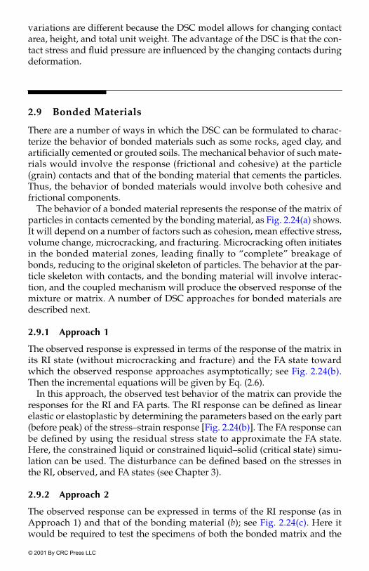
© 2001 By CRC Press LLC
variations are different because the DSC model allows for changing contactarea, height, and total unit weight. The advantage of the DSC is that the con-tact stress and fluid pressure are influenced by the changing contacts duringdeformation.
2.9 Bonded Materials
There are a number of ways in which the DSC can be formulated to charac-terize the behavior of bonded materials such as some rocks, aged clay, andartificially cemented or grouted soils. The mechanical behavior of such mate-rials would involve the response (frictional and cohesive) at the particle(grain) contacts and that of the bonding material that cements the particles.Thus, the behavior of bonded materials would involve both cohesive andfrictional components.
The behavior of a bonded material represents the response of the matrix ofparticles in contacts cemented by the bonding material, as Fig. 2.24(a) shows.It will depend on a number of factors such as cohesion, mean effective stress,volume change, microcracking, and fracturing. Microcracking often initiatesin the bonded material zones, leading finally to “complete” breakage ofbonds, reducing to the original skeleton of particles. The behavior at the par-ticle skeleton with contacts, and the bonding material will involve interac-tion, and the coupled mechanism will produce the observed response of themixture or matrix. A number of DSC approaches for bonded materials aredescribed next.
2.9.1 Approach 1
The observed response is expressed in terms of the response of the matrix inits RI state (without microcracking and fracture) and the FA state towardwhich the observed response approaches asymptotically; see Fig. 2.24(b).Then the incremental equations will be given by Eq. (2.6).
In this approach, the observed test behavior of the matrix can provide theresponses for the RI and FA parts. The RI response can be defined as linearelastic or elastoplastic by determining the parameters based on the early part(before peak) of the stress–strain response [Fig. 2.24(b)]. The FA response canbe defined by using the residual stress state to approximate the FA state.Here, the constrained liquid or constrained liquid–solid (critical state) simu-lation can be used. The disturbance can be defined based on the stresses inthe RI, observed, and FA states (see Chapter 3).
2.9.2 Approach 2
The observed response can be expressed in terms of the RI response (as inApproach 1) and that of the bonding material (b); see Fig. 2.24(c). Here itwould be required to test the specimens of both the bonded matrix and the
ch-02 Page 53 Monday, November 13, 2000 5:55 PM
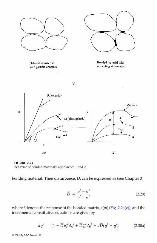
© 2001 By CRC Press LLC
bonding material. Then disturbance, D, can be expressed as (see Chapter 3)
(2.29)
where i denotes the response of the bonded matrix, a(m) (Fig. 2.24(c)), and theincremental constitutive equations are given by
(2.30a)
FIGURE 2.24Behavior of bonded materials: approaches 1 and 2.
D�
i�
a�
�i
�b
�------------------�
d�˜
a 1 D�( )C˜
id�˜
i DC˜
bd�˜
b dD �˜
b�˜
i�( ) �
ch-02 Page 54 Monday, November 13, 2000 5:55 PM

© 2001 By CRC Press LLC
where is the constitutive matrix for the bonding material, which can beassumed to be elastic, elastoplastic, elastic with disturbance, or elastoplasticwith disturbance, depending on the observed response, a(b). It may be possi-ble to assume that the (average) strains in both the matrix and the bondingmaterial are the same, i.e., � � . Then Eq. (2.30a) reduces to
(2.30b)
2.9.3 Approach 3
The bonded material (matrix) can be assumed to be composed of the skeletonof particles with contacts but without bonds (s), and the bonding material (b);see Fig. 2.25. Then the observed (incremental) response of the matrix
can be expressed as the sum of the responses, as
(2.31a)
or
(2.31b)
FIGURE 2.25Response of bonded material: approach 3.
C˜
b
d�˜
i d�˜
b d�˜
d�˜
a 1 D�( )C˜
i DC˜
b[ ]d�
˜dD �
˜b
�˜
i�( )�
d�m( )
d�m d�
s d�b
��
d�m C
˜s d�
˜s C
˜bd�
˜b
��
ch-02 Page 55 Monday, November 13, 2000 5:55 PM
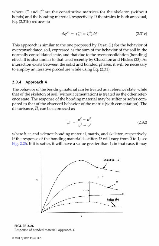
© 2001 By CRC Press LLC
where and are the constitutive matrices for the skeleton (withoutbonds) and the bonding material, respectively. If the strains in both are equal,Eq. (2.31b) reduces to
(2.31c)
This approach is similar to the one proposed by Desai (1) for the behavior ofoverconsolidated soil, expressed as the sum of the behavior of the soil in thenormally consolidated state, and that due to the overconsolidation (bonding)effect. It is also similar to that used recently by Chazallon and Hickes (23). Asinteraction exists between the solid and bonded phases, it will be necessaryto employ an iterative procedure while using Eq. (2.31).
2.9.4 Approach 4
The behavior of the bonding material can be treated as a reference state, whilethat of the skeleton of soil (without cementation) is treated as the other refer-ence state. The response of the bonding material may be stiffer or softer com-pared to that of the observed behavior of the matrix (with cementation). Thedisturbance, , can be expressed as
(2.32)
where b, m, and s denote bonding material, matrix, and skeleton, respectively.If the response of the bonding material is stiffer, D will vary from 0 to 1; seeFig. 2.26. If it is softer, it will have a value greater than 1; in that case, it may
FIGURE 2.26Response of bonded material: approach 4.
C˜
s C˜
b
d�˜
m C˜
s C˜
b�( )d�
˜�
D
D�
b�
m�
�b
�s
�--------------------�
ch-02 Page 56 Monday, November 13, 2000 5:55 PM

© 2001 By CRC Press LLC
be nondimensionalized with respect to the final value, Df, corresponding tothe residual stress so that it varies from 0 to 1. However, in that case, the valueDf needs to be provided in the analysis and computation.
Figure 2.26 indicates that the behavior of the matrix is affected by progres-sive microcracking in the bonds. In the limit, the behavior of the bondedmatrix may tend toward that of the skeleton of a (dry) granular system with-out bonds but with particle contacts. Thus, the behavior of the skeleton canbe obtained from tests with the granular material (say, sand) in its state with-out the artificial or natural bonding.
2.9.5 Porous Saturated Bonded Materials
The equilibrium of forces for a material composed of solid particle contacts,bonding material, and fluid, with areas As, Ab , and Af, respectively (Fig. 2.27),gives
(2.33a)
(2.33b)
where Ds, Db, and Df are ratios of the areas of the solid contacts, bondingmaterial, and fluid to the total nominal area A. It will be difficult to determinethe three areas in a deforming material.
If we assume that the contact area, As, is negligible and define effectivestress over the nominal area, A, as in the Terzaghi theory [Eq. (2.20)], Eq.(2.33) reduces to
(2.34)
FIGURE 2.27Saturated bonded material.
Fa
A----- Fs
As------
As
A------ Fb
Ab------
Ab
A------
F f
A f------
A f
A------ �
�a
�s Ds �
b Db �f D f �
�a
� �b
Ab
A------ p 1
Ab
A------�
�
ch-02 Page 57 Monday, November 13, 2000 5:55 PM

© 2001 By CRC Press LLC
where is the effective stress and p is the pore water pressure in the senseof the classical effective stress principle. However, as noted before, the chang-ing contact area is not included in such an approximation. Specializationsuch as in Eq. (2.34) has been used for defining the behavior of cementedsands (24).
2.9.6 Structured Materials
A structured material is defined as a material that possesses a modified micro-structure in relation to that of its basic reference state. Thus, many materialsystems such as reinforced systems (earth, concrete, and metal or ceramiccomposites), overconsolidated soil, dislocated silicon with impurities,asphalt concrete with enhanced bonding due to chemical effects, and naturalsoils with respect to their reconstituted or remolded states (25) can be treatedas structured materials. The formulation and application of the DSC for struc-tured materials are given in Chapter 10.
2.10 Characteristics of the DSC
It is evident from Eq. (2.6) that the DSC constitutive equations involve
(1) the influence of the deformation characteristics of the interactingmaterial parts in the reference states, and
(2) the possibility of relative motions (translation, rotation) betweenthe material parts in the reference states, which can involve differ-ent stresses (and strains) in them.
These two properties are important as they allow for the interactionbetween the two parts, leading to a diffusion-type process within the mixturein the material element. As a result, Eq. (2.6) can provide a general formula-tion, compared to that in the classical damage model (6, 7) in which thecracked parts are assumed to carry no stress. Various specializations of theDSC, including the classical damage model, are discussed in Chapter 4.
2.10.1 Comparisons and Comments
One of the distinguishing features of the DSC is that it allows for the interact-ing mechanisms between the parts in the reference states as affected by themicrostructural rearrangement and self-adjustment of particles. However, itsformulation does not require particle or microlevel characterization. This isbecause the responses of the parts in the reference states are defined on thebasis of the macrolevel response measured on finite-sized (laboratory) speci-mens. As a result, it avoids the necessity of defining particle-level constitutiveequations, which are required in the micromechanical and microcrack inter-
�
ch-02 Page 58 Monday, November 13, 2000 5:55 PM

© 2001 By CRC Press LLC
action (with damage) models (26). This is considered to be a distinct advan-tage, as it is difficult (at this time) to measure constitutive responses at theparticle level; therefore, in the micromechanical and microcrack interactionmodels, it is usually defined on the basis of measured behavior on finite-sizedspecimens, which is indeed an inconsistency.
Furthermore, a material made up of many (millions of) particles represents acomplex and nonlinear system. Hence, it is not possible theoretically to integrate(micro-) particle-level responses to obtain the macrolevel response because a partof the particle interactions may be lost in the process. Indeed, approximations arealways possible, as the micromechanical models imply. In the DSC, we dependon the interaction between clusters of material parts in the reference states, whichis considered to be more consistent for describing the behavior of the complexsystem. In Chapters 3 to 12 we discuss how the responses of the material parts inthe reference states are determined from laboratory tests.
It is often appropriate to define the RI behavior on the basis of plasticity theoryinvolving a yield surface. However, it is not necessary to invoke yield-surface-based model(s) in the DSC. It can be formulated on the basis of irreversiblestrains without the yield surface.
2.10.2 Self-Organized Criticality
The self-organized criticality (SOC) concept by Bak and co-workers (27)around the mid-1980s analyzes the unique collapse or catastrophic states amaterial may reach under thermomechanical loading. This concept is similarto the critical state (CS) concept of soil mechanics developed by Roscoe and co-workers in the 1960s (8, 9) in which a soil with given initial confining pressureapproaches the critical state when its density or void ratio approaches uniquevalue irrespective of its initial density. At the critical state, the material deformsin shear without a change in its volume. The synergetics concept by Haken in1978 (28) proposed a theory for analyzing the unique final state, called the “stateof thermal equilibrium” into which a system develops. Here, the original struc-ture of the system disappears, replaced by homogeneous systems.
The DSC allows the characterization of the catastrophic or collapse state asin the foregoing concepts, and also the characterization of the entire behaviorof the material including the prepeak and postpeak responses. Hence, theDSC is considered to be general compared to the SOC, CS, and synergeticsconcepts. Detailed descriptions of the SOC in comparison with the DSC, aswell as the generality of the DSC, are presented in Appendix I.
2.11 Hierarchical Framework of the DSC
Figure 2.28 depicts the unified and hierarchical framework of the DSC. It per-mits, as shown in the subsequent chapters, adoption of constitutive modelsdepending on the specific material properties for a given application’s need.
ch-02 Page 59 Monday, November 13, 2000 5:55 PM

© 2001 By CRC Press LLC
References
1. Desai, C.S., “A Consistent Finite Element Technique for Work-Softening Behav-ior,” Proc. Int. Conf. On Comp. Meth. in Nonlinear Mech., J.T. Oden (editor), Univ.of Texas, Austin, 1974.
2. Desai, C.S., “Finite Element Residual Scheme for Unconfined Flow,” Int. J. Num.Meth. Eng., 10, 1976, 1415–1418.
3. Desai, C.S. and Li, G. C., “A Residual Flow Procedure and Application for FreeSurface Flow in Porous Media,” Adv. in Water Resources, 6, 1983, 27–35.
4. Baseghi, B. and Desai, C.S., “Laboratory Verification of the Residual FlowProcedure for Three-Dimensional Free Surface Flow,” Water Resources Research,26, 2, 1990, 259–272.
5. Bruch, J.C., Jr., “Fixed Domain Methods for Free and Moving Boundary Flowsin Porous Media,” Transport in Porous Media, 6, 1991, 627–649.
6. Kachanov, L.M., Theory of Creep, English translation editor A.J. Kennedy, Na-tional Lending Library, Boston, MA, 1958.
7. Kachanov, L.M., Introduction to Continuum Damage Mechanics, Martinus NijhoftPublishers, Dordrecht, The Netherlands, 1986.
FIGURE 2.28Hierarchical versions in DSC.
ch-02 Page 60 Monday, November 13, 2000 5:55 PM

© 2001 By CRC Press LLC
8. Roscoe, K.H., Scofield, A. and Wroth, C.P., “On Yielding of Soils,” Geotechnique,8, 1958, 22–53.
9. Scofield, A.N. and Wroth, C.P., Critical State Soil Mechanics, McGraw-Hill, Lon-don, 1968.
10. Felice, C. W., Tester, V. J., and Sharer, J., “A Nondestructive Damage Assessmentof PCGC Grout,” Proc. Conf. On Containment of Underground Nuclear Explosions,Univ. of Nevada, Reno, NV, 1991.
11. Desai, C.S., “Constitutive Modelling Using the Disturbed State as Microstruc-ture Self-Adjustment Concept,” Chap. 8 in Continuum Models for Materialswith Microstructure, H.B. Mühlhaus (Editor), John Wiley, Chichester, U.K.,1995.
12. Desai, C.S. and Toth, J., “Disturbed State Constitutive Modeling Based onStress-Strain and Nondestructive Behavior,” Int. J. Solids and Structures, 33, 11,1619–1650, 1996.
13. Desai, C.S., Park, I. J., and Shao, C., “Fundamental Yet Simplified Model forLiquefaction Instability,” Int. J. Num. Analyt. Meth. in Geomech., 22, 721–748,1998.
14. Desai, C.S., “Liquefaction Using Disturbance and Energy Approaches,” J. ofGeotech. and Geoenv. Eng., ASCE, 126, 7, 2000, 618–631.
15. Scott, T.E., Azeemuddin, M., Zaman, M., and Rogiers, J. C., “Changes in Acous-tic Velocity During Pore Collapse of Rocks,” News Journal, Int. Soc. of RockMechanics, 3, 1, 1995, 14–17.
16. Owen, D.R.J. and Hinton, E.. Finite Elements in Plasticity: Theory and Practice,Pineridge Press, Swansea, UK, 1980.
17. Terzaghi, K., Theoretical Soil Mechanics, John Wiley & Sons, New York, 1943.18. Bishop, A.W. and Eldin, G., “Undrained Triaxial Tests on Saturated Sands and
Their Significance in the General Theory of Shear Strength,” Geotechnique, 2, 1,1950.
19. Perloff, W.H. and Baron, W., Soil Mechanics: Principles and Applications, TheRonald Press Co., New York, 1976.
20. Lamb, T.W. and Whitman, R. V., “The Role of Effective Stress in the Behaviorof Expansive Soils,” Report, Colorado School of Mines, 54, 4, 1959.
21. Skempton, A., “Effective Stress in Soils, Concrete and Rock,” Proc. Conf. on PorePressure and Suction in Soils, London, 1961.
22. Desai, C.S. and Wang, Z., “Disturbed State Model for Porous Saturated Mate-rials,” Int. J. Geomechanics, accepted 2000.
23. Chazallon, C. and Hickes, P. Y., 1998, “A Constitutive Model Coupling Elasto-plasticity and Damage for Cohesive-Frictional Materials,” J. of Mech. of Cohesive-Frictional Mataerials, 3(1), 41–63.
24. Abdulla, A.A. and Kiousis, P.D., 1997, “Behavior of Cemented Sands, Parts Iand II,” Int. J. Num. Analyt. Meth. Geomech., 21, 8, 533–547 and 549–568.
25. Liu, M.D., Carter, J.P., Desai, C.S., and Xu, K. J., “Analysis of the Compressionof Structured Soils Using the Disturbed State Concept,” Int. J. Num. Analyt.Meth. Geomech., 24, 8, 2000, 723–735.
26. Bazant, Z.P., “Nonlocal Damage Theory Based on Micromechanics of CrackInteractions,” J. Eng. Mech., ASCE, 120, 1994, 593–617.
27. Bak, P., How Nature Works, Copernicus (Springer-Verlag), New York, 1996.28. Haken, H., Synergetics: An Introduction, Springer-Verlag, Berlin, Germany,
1978.
ch-02 Page 61 Monday, November 13, 2000 5:55 PM

© 2001 By CRC Press LLC
3Relative Intact and Fully Adjusted States, and Disturbance
CONTENTS3.1 The Relative Intact and Fully Adjusted States
3.1.1 Characterization of Material at Critical State3.1.2 Specializations
3.2 Disturbance and Function3.2.1 Disturbance Function3.2.2 Laboratory Tests3.2.3 Stiffening or Healing3.2.4 Representation of Disturbance3.2.5 The Stiffening Effect3.2.6 Creep Behavior3.2.7 Rate Dependence3.2.8 Disturbance Based on Disorder (Entropy) and Free Energy
3.3 Material Parameters.3.3.1 Fully Adjusted State3.3.2 Disturbance Function
In Chapter 2, we derived the following incremental DSC equations (1.8) for anelement of the same material composed of material parts in RI and FA states:
(3.1a)
or, in matrix notation,
(3.1b)
Similar incremental equations can be derived for the alternative formulationsfor an element composed of more than one material, e.g., Eqs. (2.9c), (2.11),(2.14), and (2.30a) of Chapter 2.
d�ija 1 D�( )Cijk�
i d�k�i DCijk�
c d�k�c dD �ij
c�ij
i�( )� ��
�
d�˜
a 1 D�( )C˜
id�˜
i DC˜
cd�˜
c dD �˜
c�˜
i�( )� ��
Both the tensor and matrix notations are often used in this text. The latter can provide for con-venient implementation in computer procedures.�

© 2001 By CRC Press LLC
In this chapter, we present explanations for the RI (i) and FA (c) states and thedisturbance function, D, with respect to a given material. We also present proce-dures for the determination of parameters for the FA state and the disturbancefunction, D; for the RI models, they are presented in Chapters 5 to 12.
At this time, we consider disturbance that results in damage or degradation;stiffening or healing where the disturbance may decrease is discussed in Chapter10. In that case, a deforming material element experiences microstructuralchanges that result in increased disturbance from the initial disturbance, whichcan be zero or nonzero. The initial disturbance depends on the initial conditionssuch as anisotropy, flaws, dislocations, and manufacturing defects. During themicrostructural modifications and the self-adjustment of material particles, thematerial parts in the relative intact (RI) state transform to fully adjusted (FA)parts. Figure 3.1(a) shows a schematic of the growth of disturbance with loadingand deformation. The shaded zones show the FA parts, while the unshaded
FIGURE 3.1Representations of DSC.

© 2001 By CRC Press LLC
parts show clusters of the RI parts. The asymptotic value of disturbance is unitywhen the FA state is reached over the entire material element. Before the FA statecan be reached, the material’s microstructure can experience local and globalinstabilities, denoted by Dc, Df, Du, etc. [Fig. 3.1(b)–(d)], which are also discussedlater (e.g., Chapter 12). For instance, in the case of a dense granular material, alocal instability occurs when the material transits from compactive to dilativevolume (Dcd), which may not necessarily cause ‘‘failure.” However, when thecritical value of disturbance (Dc) is reached [Fig. 3.1(b)–(d)], failure in the sense ofengineering reliability can initiate, while at D � Df the material may be consid-ered to have ‘‘failed.’’ For given initial conditions (pressure, density) the behaviormay approach a residual (or critical) state (Du), which may be adopted approxi-mately as the FA state for the evaluation of the disturbance. As shown in Fig.3.1(c), the final FA state (D � 1) is not measurable because the material had“failed” before that state can be realized. However, D � 1 can also be used in theformulation of the model, for instance, in the mathematical definition of D ahead.
3.1 The Relative Intact and Fully Adjusted States
Figure 3.2 shows schematics of stress–strain responses of materials whosephysical state, defined by density (�) or void ratio (e), does not change signif-icantly during deformation. In other words, as in the case of some metals, it
FIGURE 3.1(Continued.)

© 2001 By CRC Press LLC
is assumed that the density or void ratio of the material remains invariantduring deformation. The linear elastic response can be considered to be theRI state in relation to the observed elastic–plastic (hardening) behavior. Theelastic–plastic hardening response can be treated as an RI state in relation tothe elastic perfectly plastic response. The linear elastic or the elastic–plastichardening responses can be treated as RI in relation to the observed degrada-tion or softening behavior.
In the case of granular and frictional materials like soils (clays, sands),rocks, and concrete, the observed response depends on various factors suchas initial mean pressure (p0 � �0 � J10/3), where J1 � �1� �2 � �3, density orvoid ratio (volume of void to volume of solids), and stress or loading path (3,4, 6, 7). Here the physical state defined by density or void ratio changes dur-ing deformation. Figure 3.3(a) shows schematics of the stress–strain behaviorof initially loose and dense granular materials. The loose material with initialvoid ratio , and given initial pressure (p0), compacts continuously, its voidratio decreases, and it approaches a critical value, ec, (Fig. 3.2(b) and (c)),when the stresses reach critical values and , where J2D is the secondinvariant of the deviatoric stress tensor, Sij, and is proportional to the shearstress difference (�1 � �3) and to octahedral shear stress, �oct.
The initially dense material with void ratio and a given pressure (p0)may first compact and then experience the transition at point b (Fig. 3.3(b)),corresponding to Dcd [Fig. 3.1(c)], when its volume increases or it experiencesdilation. That is, the void ratio first decreases, then increases after point b, andupon further deformation, after passing through the peak (point d), itapproaches the critical state (ec, , ); see Fig. 3.3(d). The material’sresponse at the critical state can be used to define the behavior of the materialin the FA state.
FIGURE 3.2Stress–strain behavior: no change in physical state.
e0a
J1c
J2Dc
e0a
J2Dc J1
c

© 2001 By CRC Press LLC
Relative Intact Behavior. A loose material with an initial mean pressure(p0) may compact continuously during shear loading. In that case, the RIresponse can be characterized by excluding the effect of increased compac-tion, in which case the observed response can be stiffer than the RI response[Fig. 3.3(a)].
In the case of a dense material, the initial compaction would warrantconsideration similar to that for the loose material. However, for practicalpurposes, and because for the response up to the transition point [b; Fig. 3.3(a)]
FIGURE 3.3 Behavior of loose and dense granular materials.

© 2001 By CRC Press LLC
the disturbance is usually negligible, the RI and the observed responses maybe assumed to be approximately the same (up to point b). Then internal‘‘microcracking” and relative particle motions would result in dilation, andthe disturbance (damage) after point b would increase continuously. The RIresponse thereafter can be characterized as nonlinear elastic or elastic–plastichardening (e.g., �0-model, Chapter 7) [Fig. 3.3(a)]. Details of constitutiveequations and matrix, , Eq. (3.1), that characterizes the RI response aregiven in Chapters 4 to 11.
Fully Adjusted Behavior. The material parts that have reached the FA stateduring deformation can be considered to be at the critical state, e.g., .When the material element follows the same stress path (as in a laboratory test),this (stress) state will be defined uniquely.
Further explanation of the behavior of a material element in the DSC isdepicted in Fig. 3.4(a) in the four-dimensional space, J1� , e,where I2D is the second invariant of the deviatoric strain tensor, Eij (8). Here,as a simplification, the response in which the physical state (e) does notchange during deformation is considered; examples of such a behavior are ametal and saturated soil under undrained conditions. The shear loadingstarts at point A and travels along path A–C, and the observed or averageresponse is denoted by point C. The corresponding RI and FA (critical) statesare denoted by points B and D, respectively. Similar depictions can be devel-oped for other loading conditions and stress paths.
In a boundary-value problem, on the other hand, if the stress paths for eachmaterial element (or point) can be computed, after a given incremental loading,its stress and void ratio at the critical state can be evaluated. This is shownschematically in Fig. 3.5 for three typical points (1–3) in a half-space loadedincrementally. The loadings of these points start at three different initialpressures ( J10). Points 1 and 2 may approach their critical states at and ,respectively, while point 3 may not reach the critical state at all. However,once a material point has reached the FA (critical) state during deformation,its critical state is defined with respect to the stress path followed by theoverall material element (consisting of RI and FA parts); see Fig. 3.1(a).
3.1.1 Characterization of Material at Critical State
When the material is at the critical state, there is no further change in itsvolume or void ratio, and it deforms in shear under constant value of theshear stress reached up to that state (9). Based on laboratory obser-vations, it is possible to define the behavior of the material at the critical statein terms of , and , as depicted in Fig. 3.3(d) and (e). Then the consti-tutive response of the material at the critical state can be expressed as
(3.2a)
C˜
i
ec , J2Dc , J1
c( )
J2D I2D�
1c 2c
J2Dc( )
J2Dc ,J1
c ec
J2Dc mJ1
c�

© 2001 By CRC Press LLC
and
(3.2b)
where is the slope of the critical state line (CSL) [Fig. 3.3(d)], is the slopeof the critical state line [Fig. 3.3(e)], and is the value of corresponding to
� 3pa, where pa is the atmospheric pressure constant.Then the behavior of the material, Eq. (3.2), at the critical state can be used
to define the response of the material parts in the FA state. The physical interpre-tation is that the growing clusters of the FA parts (at the critical state), Fig. 3.1(a),as they are surrounded by the RI parts, possess certain strength like a con-strained liquid–solid (CLS). That is, they can continue to carry the sameshear stress without change in volume. Thus, the deforming FA parts
FIGURE 3.4 DSC in four-dimensional space and component spaces. (From Ref. 8, with permission.)
ec e0c
�n J1c3pa( )��
me0
c ec
J1c
J2Dc( )

© 2001 By CRC Press LLC
provide interaction with the RI parts and produce the coupled observedresponse.
3.1.2 Specializations
Now, if it is assumed that the FA part (at the critical state) can carry no shearstress but can continue to carry hydrostatic stress or mean pressure, itbehaves like a constrained liquid (CL). In this case, in Eq. (3.2a) is zero.Then the constitutive equation for the FA part will depend only on the volu-metric response, Eq. (3.2b).
If the FA material is treated like a “void” or crack, as it is assumed in the clas-sical damage approach (10), it cannot carry any shear or hydrostatic stress. Then
� 0 and � 0 in Eq. (3.2a,b) and the stress point is at the origin (Fig. 3.6); thisidealization does not allow for coupling between the RI and FA parts. Figure3.6 depicts the above specializations in the �J1 and e � J1 spaces, in which
FIGURE 3.5FA (critical state) in boundary-value problems.
m
m
J2D

© 2001 By CRC Press LLC
CLS corresponds to the constrained liquid–solid, CL to constrained liquid, andvoid to no strength, idealizations. Further details on the equations for the FAstate and matrix , Eq. (3.1), that define the FA response are given in Chapters4 to 11.
The behavior of materials such as metals and alloys is not significantly influ-enced by the hydrostatic stress, and there is no significant change in their den-sity or void ratio during deformation. In other words, their response can becharacterized based mainly on the stress–strain response. For these materials,the FA response can be characterized as a constrained liquid, which can carrymean pressure but no shear stress. The perfectly plastic response of an elasto-plastic material can be considered analogous to such a characterization. Alter-natively, the material in the FA state for metallic materials can be assumed tocarry no stress at all. Some examples are given in Chapter 6.
The idea of the critical state can be considered a generalization of classicalelastoplastic theory (Chapter 6). Just as in the critical state concept, the mate-rial, like a metal whose stress–strain behavior is essentially independent ofthe mean pressure (Fig. 3.2), reaches a state of constant volume at the yield.Then the material deforms under constant yield stress.
FIGURE 3.6 Representation of FA behavior.
Cc
˜

© 2001 By CRC Press LLC
3.2 Disturbance and Function
The observed response, , is expressed in terms of the responses, and ,of the materials in the reference states, RI and FA, respectively:
(3.3)
Figure 3.1(b) shows a symbolic representation of the , , and statesconnected through the disturbance, D, which acts as an interpolation mecha-nism between the interacting materials in the RI and FA states. An approxi-mate analogy can be given here: the above representation is similar toexpressing the behavior of a given volume of the mixture of ice and water interms of the behavior of ice and water. The behavior of ice is analogous to thatof the RI material, and the behavior of water is analogous to that of the FAmaterial.
In a deforming material, disturbance, D, can be expressed as the massof material in the FA state to the total mass (M):
(3.4)
With no initial disturbance, D varies from 0 to 1, as initially , andat higher deformations . If we assume that the densities of thematerials in various states are the same, D can be expressed approximatelyas
(3.5a)
(3.5b)
(3.5c)
where , , and are the volume, area, and length of three-dimensional,two-dimensional, and one-dimensional material elements in the FA state,respectively.
Ra Ri Rc
Ri Rc� Ra⇒
Ri Ra Rc
Mc( )
DMc
M-------�
Mc 0�Mc M→
DVc
V------�
DAc
A------�
D�c
�----�
Vc Ac �c

© 2001 By CRC Press LLC
In general, however, D can be expressed as
(3.6)
where the functions D1 and D2 depend on the varying density and volume,respectively.
It may be noted that the form of D in Eq. (3.5) is similar to the damage (�)in the classical damage approach (10). However, in the DSC, the interpreta-tion of disturbance is different and general; it considers that the FA materialhas specific strength and that it interacts with the RI material. On the otherhand, in the classical damage approach, the FA material is treated as a “void”without interaction with the RI part. Furthermore, in the DSC, D can denoteboth damage or degradation, and growth or stiffening (strengthening).
3.2.1 Disturbance Function
Once the RI and FA states and disturbance are defined, the next step is to for-mulate the disturbance function, D. The development of microcracking anddamage, as well as compaction and strengthening, can depend on the direction,and hence, it would lead to anisotropic disturbance. As a result, in general, Dwould be a tensor with directional components (Chapter 2). It is usually difficultto measure the directional properties of deforming materials; some possibleways are discussed in Chapter 2. However, for practical purposes, it may oftenbe sufficient to treat D as a scalar, in an average and weighted sense. Most of thedescriptions in this text treat D as a scalar.
There are a number of ways in which we can define D to represent degra-dation or strengthening. The most direct way is to measure the mass, volume,etc. [Eqs. (3.4) and (3.5)] of the material in the FA state. However, this can bedifficult at this time, mainly because of the lack of proper testing devices topenetrate the material and measure these quantities; additional discussion onthis aspect is presented in Chapter 2. Hence, the indirect approaches need tobe developed based on phenomenological considerations. One such indirectway is to define D from the measurements of stress–strain (� ��), volumetric(void ratio), effective stress , or pore water pressure (p) andor nonde-structive responses; see Fig. 3.7(a) to (d). The other phenomenological way isto express D in terms of (internal) variables such as plastic strain trajectory,and plastic work or dissipated energy. The definition of D usually relies onthe combination of these two phenomenological approaches.
3.2.2 Laboratory Tests
The disturbance that expresses the deviation of the observed behavior withrespect to its behavior in the two reference states, RI and FA, can be defined onthe basis of the stress–strain, volumetric (void ratio), and nondestructive
D�
c
�---- Vc
V------� D1 D2�� �
�( )

© 2001 By CRC Press LLC
(velocity or attenuation) behavior. Figure 3.7(a) and (b) show typicalstress–strain and void ratio (volumetric) responses. The disturbance, D, can beexpressed as
(3.7a)
FIGURE 3.7Disturbance from test data.
D�
�i
�a
�
�i
�c
�------------------�

© 2001 By CRC Press LLC
and
(3.7b)
where � denotes appropriate stress measures such as axial stress �1, shearstress �, stress difference (�1��3); �
, where �i (i �1, 2, 3) are the principal stresses, or octahedral shearstress, . It may be noted that values of D� and De at a givenstage during deformation may not be the same. However, in the iterativesolution procedures, both the stress equilibrium and volumetric responsescan be satisfied simultaneously (Chapter 13).
Often, the disturbance can be defined in terms of and the measure ofhydrostatic or mean stress, J1, as
(3.8a)
(3.8b)
Then they can be used in the constitutive Eqs. (3.1), which are decomposedin deviatoric and hydrostatic components. The use of such a decompositionfor the behavior of interfaces is given in Chapter 11.
In the case of the nondestructive behavior, say, ultrasonic or Lamb wavevelocity (V), the disturbance can be expressed as [Fig 3.7(c)]
(3.9)
where Dv is disturbance based on velocity, is the velocity in the RI state,which can be adopted as the velocity in the initial state of the material, isthe observed velocity, and is the velocity in the FA state, which can beadopted as the asymptotic value to the observed response (5, 11).
In the case of undrained behavior, when the liquid from a saturated porousmaterial does not have sufficient time to drain (under static or cyclic loading),the disturbance can be obtained in various ways; for strain-controlled tests,see Fig. 3.8, or for stress-controlled tests, see Fig. 3.9 (12).
In the case of the strain-controlled test, the disturbance, D�, can be foundby using Eq. (3.7), in which peak stresses for different cycles are used as theobserved response. Here the continuation of the response under the firstcycle, not affected by cyclic degradation, can be treated as the RI response
Deei ea
�
ei ec�
---------------�
J2D(J2D � 16[ �1 �2�( )2�2 �3)�
2�
�3 �1)�2 ]
�oct 23 J2D�
J2D
D J2D
i J2Da
�
J2Di J2D
c�
-------------------------------�
D J1
i J1a
�
J1i J1
c�
-------------------------�
DV
Vi Va�
Vi Vc�
--------------------�
Vi
Va
Vc

© 2001 By CRC Press LLC
(e.g., using HISS �0 -plasticity model; Chapter 7). The residual or ultimatestress ( ) can be adopted as the stress in the FA state; see Fig. 3.8(a).
For the stress-controlled loading, Fig. 3.9(a), the extension of first-cyclebehavior can be treated as the RI response simulated by using a suitable model,e.g., the HISS �0-model. Based on the pore water pressure measurements, theobserved mean effective stress can be found as
(3.10)
where and �i (i �1, 2, 3) are the effective and total stresses, respectively,and p is the pore water pressure.
FIGURE 3.8 Cyclic strain-controlled test.
�c
�( )a�1 �2 �3� �( )a
3 �1 �2 �3 3p�� �( )a3� �
�i

© 2001 By CRC Press LLC
The integration of the incremental plasticity equations for the �0-model(Chapter 7)
(3.11)
leads to the computation of the RI stresses and the value of for the RIresponse. A schematic of and vs. the number of cycles (N) or corre-sponding deviatoric plastic strain trajectory, �D, from Fig. 3.9(a), is shown inFig. 3.7(d). Then the disturbance based on the effective stress can be evaluated
FIGURE 3.9Cyclic stress-controlled test.
d�˜
i C˜
i ep( )d� �˜
i
�( )i
�( )i�( )a

© 2001 By CRC Press LLC
as (12,13)
(3.12a)
where denotes the measured ultimate (asymptotic) value. Alternatively,the measured excess pore water pressure can be used as [see Fig. 3.9(b)]
(3.12b)
where is the initial effective confining stress . Further details includinginstability and liquefaction analysis are given in Chapter 9.
3.2.3 Stiffening or Healing
Some materials, e.g., saturated sands during deformation in the post-lique-faction zone, dislocated silicon crystals with impurities (oxygen, nitrogen,etc.), and asphalt in pavements, may experience a strengthening responseduring loading and unloading. Some reasons for such “healing” are continu-ing compaction, chemical rebonding, and locking of dislocations. A sche-matic of the stress–strain response showing softening and stiffening is shownin Fig. 3.10. Here, disturbance can be expressed using Eq. (3.7). However, it
FIGURE 3.10 Softening and stiffening behavior.
D�
�( )i�( )a
�
�( )i�( )c
�----------------------------�
�( )c
Dp
pa
pi----�
pi�0

© 2001 By CRC Press LLC
may first increase due to microcracking and softening, and then after thethreshold plastic deformation (�t), it may decrease. Details are given subse-quently here and in Chapter 10.
Disturbance from Elastic Moduli. Often, disturbance, D, can be foundapproximately on the basis of the degrading (secant) elastic (E) or shear (G)moduli. For instance, consider the shear stress (� or �12) vs. shear strain (� or �12)response in which the changing (degrading) shear modulus, G, is measuredwith deformation; see Fig. 3.11. The special form of Eq. (3.1), by ignoring the lastterm, is given by (5)
(3.13a)
where and denote the initial and FA shear moduli, respectively. If it isassumed that and that the FA state does not carry anyshear stress; that is, , Eq. (3.13a) reduces to
(3.13b)
which leads to the expression for the degrading shear modulus, , as
(3.13c)
Similarly, for the case of Young’s elastic modulus, E,
(3.13d)
FIGURE 3.11Disturbance from shear modulus.
d�12a 1 D�( )Gid�12
i� DGcd�12
c�
Gi Gc
d�12a d�12
i d�12c
� �Gc 0�
d�12a 1 D�( )Gid�12
a�
Ga
G a 1 D�( )G i�
E a 1 D�( )E i�

© 2001 By CRC Press LLC
Then the disturbance can be found as
(3.13e)
or
(3.13f)
Such values of D are considered to be approximate, because they may notinclude multidimensional effects like in the definitions when they areexpressed in terms of total plastic strain trajectory or dissipated work (seebelow).
3.2.4 Representation of Disturbance
The disturbance function, D, can be expressed in terms of certain internalvariables and factors that affect the constitutive behavior. For example, D canbe expressed as
(3.14a)
where � denotes an internal variable such as the plastic strain trajectory, w isthe (dissipated) energy, S is entropy (disorder), � is free energy, t is time orthe number of loading cycles (N), T is temperature, and �i (i � 1, 2, …)denotes factors like environmental (chemical) effects and impurities. As asimplification, D can be written as
(3.14b)
or
(3.14c)
where � or w is affected by time, temperature, and �i. Often, the internalmicrostructural changes are assumed to be influenced mainly by the shear ordeviatoric plastic strain trajectory, �D; hence,
(3.15)
In the functional form, D is often defined by using Weibull (14) functions as
(3.16a)
DGi Ga
�
Gi-------------------�
DEi Ea
�
Ei------------------�
D D �, w, S, �, t N( ), T , �i[ ]�
D D � t,T ,�i( )[ ]�
D D w t,T ,�i( )[ ]�
D D �D, t,T ,�i( )[ ]�
D Du 1 1�D
h-----
W
�
s�
��

© 2001 By CRC Press LLC
where h, , s, and Du are material parameters. This form can provide a gen-eral variation of D, to cover materials that may undergo disturbance from thebeginning of loading, and also those that involve insignificant disturbance inthe beginning; see Fig. 3.12 (5). At the same time, D in Eq. (3.16a) can often besensitive to small changes in the parameters.
A simpler form of D commonly used is given by
(3.16b)
where A, Z, and Du are material parameters. With only two parameters, h ands (i.e., w � 0), Eq. (3.16a) can yield results similar to those from Eq. (3.16b).Note that, as discussed in Chapter 2, the expressions for D, Eqs. (3.16a and b)for the disturbance (damage) are also relevant to describe decay and growthprocesses in many natural systems.
The parameters, say A, Z, and Du in Eq. (3.16), can be expressed in terms ofsuch factors as initial confining pressure (�0), initial density (� 0), size ratio(Ld), where L is the length or height of the test specimen (material element)and d is the mean diameter; temperature (T), and initial dislocation density(N0) (15–18).
Regarding the size ratio, consider the uniaxial test results in Fig. 3.13 for anartificial rock (15); the initial value of �0( � 0), density �0, and T (room tem-perature) are assumed to be invariant. It can be seen that the stress–strainresponse is dependent on Ld. Hence, A, Z, and Du are dependent on Ld.Thus, the inclusion of Ld in the description of D can allow incorporation ofthe size effect in the DSC formulation (15, 17).
FIGURE 3.12Schematic of disturbance function (5). (With permission from Elsevier Science.)
w
D Du 1 A�Dz
�( )exp�[ ]�

© 2001 By CRC Press LLC
3.2.5 The Stiffening Effect
The disturbance function, D, Eq. (3.16), can be modified to include the stiff-ening effect, as (Fig. 3.10) (18,19)
(3.17)
where , Ab, and Zb are parameters for the softening behavior to the loweryield or residual stress, and , Ah, and Zh are parameters related to the stiff-ening response; here, is given by
(3.18)
where is the ultimate disturbance corresponding to the limiting stiffeningresponse, and is the threshold value of the deviatoric plastic straintrajectory when stiffening initiates; see Fig. 3.10. Further details are given inChapter 10.
3.2.6 Creep Behavior
In the case of the viscoplasticity (Chapter 8), the disturbance can be obtainedon the basis of the elastoplastic response. In the viscoplastic model, the time-dependent (incremental) viscoplastic response converges to the corresponding
FIGURE 3.13Stress–strain behavior of soft rock for different Ld ratios, d� 3.0 inch:(a) vs. �D; (b)D vs. �D (15). (©1990, John Wiley & Sons Ltd. Reproduced with permission.)
J2D
D Dub 1 Ab�D
Zb�( )exp�{ } 1 Ah�DZh�( )exp�{ }�[ ]�
Dub
0 if �D �Dp,�
Duh
Dub
------ if �D �Dp
�
Duh
�Dp
��t( )

© 2001 By CRC Press LLC
plastic strains according to inviscid plasticity (e.g., classical or HISS-�0 models;Chapters 6 and 7). Thus, the elastoplastic response can provide the RIresponse with respect to the observed elastoplastic (softening) behavior; seeFig. 3.14. Then the disturbance, D, can be expressed as
(3.19a)
where ξvp is the strajectory of viscoplastic strains, or
(3.19b)
where w is the dissipated energy
(3.20)
and D, A, and � are corresponding parameters. Here, is the vector of vis-coplastic strains. For materials that experience both viscoelastic and visco-plastic deformations, the energy can be expressed as
(3.21)
FIGURE 3.14Viscoplastic response:d�
vp d�p.�
D Du 1 eA�vp
Z
�( )�
D Duw 1 eAwW
Zw
� �
w �˜
d�˜
vp��
�˜
vp
w �˜
d�˜
ve d�˜
vp�( )��

© 2001 By CRC Press LLC
where is the vector of viscoelastic strains. The viscoelastic and viscoplas-tic strains in Eq. (3.21) and the parameters in Eq. (3.19) can be dependent ontemperature and other (environmental) factors. Details of creep or elastovis-coplastic models are given in Chapter 8.
3.2.7 Rate Dependence
In the case of rate-dependent behavior, the disturbance can be defined basedon stress–strain responses under different strain or deformation rates.Figure 3.15 shows a schematic of the stress–strain responses at different strainrates at a given temperature. Then the response under the highest strainrate can be assumed to represent one reference (RI) behavior, and thatunder the lowest strain or static condition can be considered as theother reference (FA) state. Then the disturbance can be expressed as
(3.22)
where , , and are the stresses corresponding to the highest strain rate,the observed, and the lowest strain rate, respectively. In terms of the irrevers-ible (plastic) strains or dissipated energy, D can be expressed as
(3.23a)
FIGURE 3.15Responses under different strain rates .�( )
�˜
ve
�( ) �( )
���( )� 0�( )
D�
i�
a�
�i
�c
�------------------�
�i�
a�
c
D Du 1 eA�D
Z
�( )�

© 2001 By CRC Press LLC
or
(3.23b)
where �D and w are the temperature-dependent deviatoric plastic or viscoplas-tic strain trajectory and dissipated energy, respectively, for a given strain rate.Then the parameters Du, A, and Z can be expressed as functions of the strainrate and temperature. Examples of temperature- and strain-rate-dependentbehavior are given in later chapters (e.g., Chapter 8).
3.2.8 Disturbance Based on Disorder (Entropy) and Free Energy
A deforming material can be considered to be composed of ordered and dis-ordered material parts. In this context, disturbance (D), which connects thetwo states, can be related to free energy and disorder. Energy can beexpressed in terms of Peirel’s and Helmholtz free energy, and disorder canbe measured in terms of entropy (20–22). Boltzmann (20) proposed the connec-tion between disorder and entropy as
(3.24)
where is the entropy, k is Boltzmann’s constant, and W is the disorderparameter, which represents the probability that the system would exist inthe state relative to all possible states in which it can exist.
Desai et al. (18) and Dishongh and Desai (19) developed a connectionbetween disturbance and rate of dislocation density, , expressed as (23, 24)
(3.25a)
where k is Boltzmann’s constant, is the back stress, Q is Peirel’s energy,, p, and r are material constants, k0 � B0/�0, B0 is mobility, T is the absolute
temperature, �0 is the (resolved) shear stress, and is the observed shearstress. The expression of D, in Eq. (3.8), by assuming � 0, gives
(3.26)
hence, the relation between and D is given by (18, 19)
(3.25b)
D Duw 1 eAwW
Zw
� �
S k ln W�
S
Nm
Nm KNmk0 J2Da
Nm�( )p r�
e QKT ��
Nm
KJ2D
a
J2Dc
J2Da 1 D�( ) J2D
i�
Nm
Nm KNmk0 1 D�( ) J2Di
Nm�p r�
e Q KT ��

© 2001 By CRC Press LLC
Basaran and Yan (25) proposed an expression for disturbance in terms ofdisorder and Helmholtz free energy (�) per unit mass given by
(3.27)
where e is the internal energy, T is the absolute temperature, and S is theentropy. The change in disorder, �W, at any time is expressed as
(3.28)
where N0 is Avogardo’s number at reference disorder, W0, is the specificmass (gmole) (26), and e0 and �0 are the internal and Helmholz free energiesat the reference state. Then disturbance, D, is expressed as
(3.29a)
If it is assumed that the temperature change ∆T is small, Eq. (3.29a) can besimplified as
(3.29b)
Equation (3.29) is similar to Eq. (3.19), which is expressed in terms ofaccumulated (deviatoric) plastic strains or dissipated energy. Equation(3.29) can provide an alternative way to express D, while the two in Eq.(3.19) can be relatively simple, particularly from the viewpoint of the definitionand determination of parameters from standard laboratory tests on materials.
3.3 Material Parameters
It is necessary to determine material parameters in the RI , FA , Eq. (3.1),characterizations, and the disturbance function. Appropriate laboratory andorfield tests on the material under various significant factors such as initial condi-tions, stress paths, volume change response, loading (static, quasistatic, cyclic,repetitive), rate of loading, temperature, and chemicals are required for the deter-mination of the parameters. Detailed descriptions of the test equipment arebeyond the scope of this book; however, we shall mention the test devicesemployed to obtain the observed behavior used for the determination ofparameters and validation of the models. Details of the determination of
� e TS��
�W W0 W� e
e0 �0�
N0kT ms------------------------
ee ��
N0kT ms------------------------
�� �
ms
D�WW0---------- 1 e�
�e0 �0�
N0kT ms------------------------ e ��
N0kT ms------------------------�
� �
D 1 e�
��e ���N0kT ms
----------------------------
�
C˜
i( ) C˜
c( )

© 2001 By CRC Press LLC
parameters and validations for various models to characterize the RIresponse are given in Chapters 5 to 12. Here, we provide the procedure fordetermination of parameters for the FA state and the disturbance function.
3.3.1 Fully Adjusted State
FA as void. If the FA state is treated as a “void” and carries no hydrostatic(mean) and shear stress, the matrix, Eq. (3.1), is null. Then it is not necessaryto have any parameters for the FA state.
FA as constrained liquid. If the FA state can carry hydrostatic stress andno shear stress and compatibility of strains is assumed, Eq. (3.1) reduces to[see Eq. (4.28)], with the associated assumptions
(3.30)
For this specialization, the DSC characterization involves only the RIresponse, that is, the model used for the RI response can be modified to simu-late the FA response. Equation (4.19) in Chapter 4 presents such a specializationof the RI constitutive matrix for the characterization of the FA behavior.
FA as critical state. If the FA behavior is characterized by using the criti-cal state concept, the parameters are those in Eq. (3.2). Their determination isdiscussed below.
At least three shear tests, triaxial with cylindrical specimens or multiaxialwith cubical specimens, with different initial confining pressures (�0��0�J103) are recommended to obtain the plots, such as in Fig. 3.3(a), (b), (d), and(e). Usually, conventional triaxial tests (�1 � �2 � �3) are performed under thestress path (CTC); see Fig. 3.16. Sometimes tests with other stress paths (see Fig.3.16) are available and can be used. The state of stress (�1 ��3) in the zoneswhere the behavior approaches the critical state provides the approximate val-ues of stress at the critical state. Note that the laboratory measurements canprovide approximate values because before the final value is reached, thematerial “fails.”
The knowledge of σ1, σ2 � σ3 at the critical state can now be used to evalu-ate from
(3.31a)
and from
(3.31b)
Then the slope of the average line on the plot and [shown in Fig.3.3(d)] yields the value of .
The values of the void ratio (see Fig. 3.3(b)) at the critical stress state(above) are available from the tests under different initial mean pressures.
C˜
c
d�ija 1 D�( )Cijk�
i d�k�i
�13--- J1
i�ij dDSij
i��
J2Dc
J2Dc 1
6--- �1 �2�( )2
�2 �3�( )2�3 �1�( )2
� �[ ]c
�
J1c
J1c
�1 �2 �3� �( )c�
J2Dc J1
c
mec( )

© 2001 By CRC Press LLC
The plot of vs. [Fig. 3.3(e)] provides the value of as the slopeof average line. Here pa is the atmospheric pressure constant. The value of ,from Eq. (3.2b), is obtained from the same plot corresponding to .
3.3.2 Disturbance Function
Let us first consider the disturbance function, D, from Eq. (3.16b), which isexpressed as follows by taking the logarithm twice:
(3.32)
FIGURE 3.16Representation of stress paths: (a) principal stress space; (b) projections of stress paths ontriaxial plane; (c) stress paths in octahedral plane.
ec ln J1c3pa( )
e0c
J1c3pa�1
Zln �D( ) ln A( ) ln lnDu D�
Du-------------------
���

© 2001 By CRC Press LLC
The value of �D, say, at any point P (see Fig. 3.17(a)) is obtained from
(3.33a)
where is the vector of the increments of plastic deviatoric strains:
(3.33b)
(3.33c)
The disturbance, Dσ, at point P is evaluated by using Eq. (3.7), and Du
corresponds to the residual (or critical) stress state, seen in Fig. 3.17. Now,a plot of ln[�ln((Du � D)Du)] vs. ln�D [Fig. 3.17(b)] provides the value of
FIGURE 3.17Determination of disturbance parameters.
�D E˜
pd E˜
pd�( )1/2��
dE˜
p
dE˜
p d�˜
p 13---�v
pI˜
��
d�˜
p d�˜
d�˜
e��

© 2001 By CRC Press LLC
Z as the slope of the average line, and the intercept along the ordinatewhen ln(�D)�0 gives the value of A.
The parameters (h, , s) in the general form, as in Eq. (3.16a), can be eval-uated by using an iterative procedure in which initial estimates are refinedprogressively; for example, the Marquard–Levenberg (ML) method, given inPress et al. (27, 28) can be used:
Let us first assume that s �1; then Eq. (3.16a) can be written as
(3.34)
The values of D and �D are evaluated at different points on a givenstress–strain curve, and Du is computed from the residual stress value[Fig. 3.17(a)]. Often, Du� 1 can be adopted. A plot of vs.ln(�D) leads to the first estimates of and from the slope and theintercept; see Fig. 3.18(a). Now the value of corresponding to the first
FIGURE 3.18Parameters for disturbance; Eq (3.15b). (Adapted from Refs. 5 and 28.)
w
lnDu
Du D�-------------------
wln�D wlnh��
ln D Du D�( )( )w� h�
s�

© 2001 By CRC Press LLC
estimates, and , can be found by writing Eq. (3.16a) as
(3.35)
A plot vs. gives the first estimate of asthe slope of the average line (Fig. 3.18(b)). The above procedure is repeated(in the ML scheme) to obtain progressively refined values of h, w, and s.
References
1. Desai, C.S., “Further on Unified Hierarchical Models Based on AlternativeCorrection or Disturbance Approach,” Report, Dept. of Civil Eng. & Eng.Mechs., University of Arizona, Tucson, AZ, USA, 1987.
2. Desai, C.S. and Ma, Y, “Modelling of Joints and Interfaces Using the DisturbedState Concept,” Int. J. Num. and Analyt. Methods in Geomech., 16, 9, 1992, 623–653.
3. Desai, C.S., “Constitutive Modelling Using the Disturbed State as Microstruc-ture Self-Adjustment Concept,” Chap. 8 in Continuum Models for Materials withMicrostructure, H.B. Mühlhaus (Editor), John Wiley, Chichester, U.K., 1995.
4. Desai, C.S., “Hierarchical Single Surface and the Disturbed State ConstitutiveModels with Emphasis on Geotechnical Applications,” Chap. 5 in GeotechnicalEngineering, K.R. Saxena (Editor), Oxford & IBH Pub. Co., New Delhi, India,1994.
5. Desai, C.S. and Toth, J., “Disturbed State Constitutive Modeling Based onStress–Strain and Nondestructive Behavior,” Int. J. Solids & Structures, 33, 11,1619–1650, 1996.
6. Wathugala, G.W. and Desai, C.S., “Damage Based Constitutive Model forSoils,” Proc. 12th Congress on Appl. Mech., Ottawa, Canada, 1989.
7. Armaleh, S.H. and Desai, C.S., “Modelling and Testing of Cohesionless MaterialUsing the Disturbed State Concept,” Int. J. Mech. Behavior of Materials, 5, 1994,279–295.
8. Katti, D.R. and Desai, C.S., “Modeling and Testing of Cohesive Soil UsingDisturbed State Concept,” J. of Eng. Mech., ASCE, 121, 5, 1995, 648–658.
9. Schofield, A.N. and Wroth, C.P., Critical State Soil Mechanics, McGraw-Hill,London, UK, 1968.
10. Kachanov, L.M., Introduction to Continuum Damage Mechanics, Martinus NijhoftPublishers, Dordrecht, The Netherlands, 1986.
11. Desai, C.S., “Evaluation of Liquefaction Using Disturbed State and EnergyApproaches,” J. of Geotech. and Geoenv. Eng., ASCE, 126, 7, 2000, 618–631.
12. Desai, C.S., Park, I.J., and Shao, C., “Fundamental Yet Simplified Model forLiquefaction Instability,” Int. J. Num. Analyt. Meth. Geomech., 22, 1998, 721–748.
13. Desai, C.S., Shao, C., and Park, I.J., “Disturbed State Modelling of Cyclic Behaviorof Soils and Interfaces in Dynamic Soil-Structure Interfaces,” Proc. 9th Int. Conf.On Computer Methods and Adv. in Geomech., Wuhan, China, 1997.
w� h�
ln 1DDu------�
s�ln 1�D
h�----- w�
���
ln 1 DDu�( ) ln[1 �Dh�( )w�
]� s�

© 2001 By CRC Press LLC
14. Weibull, W.A., “A Statistical Distribution Function of Wide Applicability,”Applied Mechanics, 18, 1951, 293–297.
15. Desai, C.S., Kundu, T., and Wang, G., “Size Effect on Damage Parameters forSoftening in Simulated Rock,” Int. J. Num. Analyt. Methods in Geomech., 14, 1990,509–517.
16. Desai, C.S., Chia, J., Kundu, T., and Prince, J., “Thermomechanical Responseof Materials and Interfaces in Electronic Packaging: Parts I and II,” J. of Elect.Packaging, ASME, 119, 4, 1997, 294–300; 301–309.
17. Desai, C.S., Basaran, C., and Zhang, W., “Numerical Algorithms and MeshDependence in the Disturbed State Concept,” Int. J. Num. Methods in Eng., 40,16, 1997, 3059–3083.
18. Desai, C.S., Dishongh, T., and Deneke, P., “Disturbed State Constitutive Modelfor Thermomechanical Behavior of Dislocated Silicon with Impurities,” J. ofAppl. Physics, 84, 11, 1998.
19. Dishongh, T.J. and Desai, C.S., “Disturbed State Concept for Materials andInterfaces with Application in Electronic Packaging,” Report to NSF, Dept. ofCivil Engng. and Engng. Mechanics, University of Arizona, Tucson, AZ, USA,1996.
20. Boltzmann, L., Lectures on Gas Theory, University of California Press, S. Brush(translator), 1998, 1964.
21. Prigogine, I. and Stengers, I., Order out of Chaos: Man’s New Dialogue with Nature,Bantam Books, New York, 1984.
22. Halliday, D. and Resnick, R., Physics, John Wiley & Sons, New York, 1966.23. Haasen, P., in Dislocation Dynamics, edited by A.R. Rosenfield et al., Battle
Institute Materials Science Colloquia, 1967; McGraw-Hill, New York, 1968.24. Dillon, D.W., Tsai, C.T., and De Angelis, R.J., “Dislocation Dynamics During
the Growth of Silicon Ribbon,” J. of Applied Physics, 60, 5, 1986, 1784–1792.25. Basaran, C. and Yan, C.Y., “A Thermodynamic Framework for Damage Mechan-
ics of Solder Joints,” J. of Electronic Packaging, ASME, 120, 4, 1998, 379–384.26. Dunstan, S., Principles of Chemistry, Van Nostrand Reinhold Co., New York,
1968.27. Press, W.H., Plannery, B.P., Teukolsky, S.A., and Vetterling, W.T., Numerical
Recipes in Pascal, Cambridge Univ. Press, Cambridge, U.K., 1986.28. Toth, J. and Desai, C.S., “Development of Lunar Ceramic Composites, Testing
and Constitutive Modeling Including Cemented Sand,” Report, Dept. of CivilEngng. and Engng. Mechanics, University of Arizona, Tucson, AZ, 1994.

© 2001 By CRC Press LLC
4DSC Equations and Specializations
CONTENTS4.1 Relative Intact Response
4.1.1 Fully Adjusted Response4.2 Specializations of DSC Equations
4.2.1 Linear Elastic4.2.2 Elastoplastic4.2.3 Elastoviscoplastic4.2.4 Thermal Effects4.2.5 Disturbance Models4.2.6 Classical Continuum Damage Model4.2.7 DSC Model Without Relative Motions4.2.8 Critical-State Characterization for FA Response4.2.9 DSC Equations with Critical State
4.3 Derivation of Strain Equations4.3.1 Strain Equations Using Critical State
4.4 General Formulation of DSC Equations4.5 Alternative Formulations of DSC4.6 Examples
In Chapter 2 we derived the following equations:
(4.1)
(4.2)
As discussed earlier, the DSC involves different stresses and strains in the material parts in the RI and FA states, respectively; see Fig. 4.1.
The latter causes relative motions or a diffusion-type process between thematerial parts in the RI and FA states. As a simplification, we can express arelationship between the strains in the RI and FA parts as [Fig. 4.1(b)]
(4.3)
�ija 1 D�( )�ij
i D�ijc
��
d�ija 1 D�( )d�ij
i Dd�ijc dD �ij
c�ij
i�( )� ��
1 D�( )Cijk�i d�k�
i DCijk�c d�k�
c dD �ijc
�iji
�( )� ��
�ijj , �ij
c( )�ij
i , �ijc( )
d�ijc Iijk� �ijk��( ) d�k�
i�

© 2001 By CRC Press LLC
where Iijk� is the unit tensor and �ijk� is the relative motion tensor. If the mate-rial is assumed isotropic and D is considered to be a weighted (average)value, � can be expressed as a scalar as
� � wD (4.4)
where w is a parameter. Then Eq. (4.3) becomes
(4.5)
Here � � wD, where 0 � D � 1 and w � 0. With the above definition of therelative motion parameter between the RI and FA strains, the first two termsin Eq. (4.2) can be expressed in terms of the RI strains, .
Now consider dD in the third term in Eq. (4.2):
(4.6)
where D is expressed in terms of D [see Eq. (4.13a) ahead]. Also
(4.7)
FIGURE 4.1Stresses and strains in RI, FA, and observed states: the randomly distributed RI and FA partsare shown as collected together.
d�ijc 1 ��( )d�ij
i�
d�iji
dD dDdD--------- dD�
dD
dD
dEijp
--------- dEijp
�
dD dEijp dEij
p( )1�2
�
d�ijp
� F �ij---------�
d�iip
� F
�kk----------�ij�
dEijp d�ij
p 13--- d�kk
p�ij��

© 2001 By CRC Press LLC
where F is the yield function in the plasticity model, e.g., F in the HISS �0-model (Chapter 7). Therefore,
(4.8)
and
(4.9a)
(4.9b)
Now,
(4.10)
and
because �ij �ij � �ii � 3. Therefore,
(4.11)
The parameter � in Eq. (4.10) is given by (see Chapter 7)
(4.12)
Now, recall that D can be expressed as [Eq. (3.19a), Chapter 3]
(4.13a)
Therefore,
(4.13b)
dEijp
� F �ij--------- 1
3--- F
�kk----------�ij�
�
dD � F �ij--------- 1
3--- F
�kk----------�ij�
F �ij--------- 1
3--- F
�kk----------�ij�
1�2
�
� F �ij--------- F
�ij---------
23--- F
�ij---------
F �kk----------�ij�
19--- F
�kk---------- �ij
F �kk----------�ij�
1�2
�
23---�
F �ij--------- F
�kk----------�ij
23--- F
�ij--------- F
�kk----------�ij for i j���
0 for i j��
19--- F
�kk----------�ij
F �kk---------- �ij
39--- F
�ii--------- F
�kk----------�
dD � F �ij--------- F
�ij--------- 1
3--- F
�ii---------
F �kk----------�
1�2
�
�
F �ij--------- Cijk�
e d�k�i
F �ij---------Cijk�
e F �k�------------ F
------
F �ij--------- F
�ij---------
1�2
�
----------------------------------------------------------------------------�
D Du 1 eA D
Z�
�( )�
dDdD--------- DuAZD
Z�1eAD
Z�
�

© 2001 By CRC Press LLC
Substitution of Eqs. (4.11) and (4.13b) in Eq. (4.6) leads to
(4.14a)
or
(4.14b)
Now, the DSC equations (4.1) become
(4.15a)
or
(4.15b)
or
(4.15c)
Here, is the constitutive tensor given by
(4.16a)
or in matrix notation:
(4.16b)
4.1 Relative Intact Response
The RI response given by in Eq. (4.2) can be defined by using elastic,elastoplastic, elastoviscoplastic, etc., characterizations. For example, considerthe �0-version of the HISS plasticity model (Chapter 7) in which the yieldfunction, F, is given by
(4.17)
dDDuAZD
Z�1eAD
Z�
( ) F �mn------------ Cmnpq
e F �ij--------- F
�ij---------
13--- F
�ii--------- F
�ii---------�
1�2
F �mn------------Cmnpq
e F �pq
----------- F ------
F �mn------------ F
�mn------------
1�2
�
------------------------------------------------------------------------------------------------------------------------------------------- d�pqi
�
dD Rpqd�pqi
�
d�ija 1 D�( )Cijk�
i ep( ) D 1 ��( )Cijk�c
�[ ]d�k�i R� k�d�k�
i�ij
c�ij
i�( )�
d�ija 1 D�( )Cijk�
i ep( ) D 1 ��( )Cijk�c R� � k� �ij
c�ij
i�( )[ ]d�k�
i�
d�ija Cijk�
DSC d�k�i
�
Cijk�DSC
Cijk�DSC 1 D�( )Cijk�
i ep( ) D 1 ��( )Cijk�c
�ijc
�iji
�( )Rk�� �[ ]�
C˜
DSC 1 D�( )C˜
i ep( ) D 1 ��( )C˜
c�˜
c�˜
i�( )R
˜T
� �[ ]�
Cijk�i
F J2D � J 12
� J 1n
�( ) 1 �Sr�( ) 0.5�� 0� �

© 2001 By CRC Press LLC
where �, n, and � are material parameters, � is the hardening or growth func-tion, � J2D/ , � , R is the bonding stress, Sr � J3D . Then the constitutive equation for the RI part with the plasticitymodel is given by
(4.18a)
or
(4.18b)
where
(4.18c)
or in matrix notation:
(4.18d)
4.1.1 Fully Adjusted Response
If it is assumed that the FA parts carry only the hydrostatic stress and noshear stress (other characterizations have been discussed in Chapter 3) andthat the FA can be characterized by using the elastoplastic RI response, theconstitutive matrix can be expressed as
(4.19a)
J2D pa2 J 1 J1 3R�( )�pa 27�2( )
J2D3�2�
d�iji Cijk�
i ep( ) d�k�i
�
d�˜
i C˜
i ep( ) d�˜
i�
Cijk�i ep( ) Cijk�
eCijmn
e F �mn------------ F
�uv----------- Cuvk�
e
F �ij---------Cijk�
e F �k�------------ F
----- F
�k�------------
F �k�------------
1�2
�
---------------------------------------------------------------------------------��
C˜
i˜
ep( ) C˜
eC˜
e F �
˜
--------- F
�˜
---------
T
C˜
e
F �
˜
------- C˜
e F �
˜
------- F ----- F
�˜
---------
T F �
˜
-------1�2
�
---------------------------------------------------------------------------��
C˜
c
C˜
cC˜
i ep( )
C1 C2 C3 0 0 0
C1 C2 C3 0 0 0
C1 C2 C3 0 0 00 0 0 0 0 00 0 0 0 0 00 0 0 0 0 0
� �

© 2001 By CRC Press LLC
where
and Cij are the components of the elastoplastic matrix, . If the FAresponse is assumed to be linear elastic, � � � K, which is the bulkmodulus.
Hence, the DSC equations are given in matrix notation as
(4.19b)
(4.19c)
Note that in Eq. (4.19b), the observed or average stress increment is expressedin terms of the strain increment in the RI part. As discussed subsequently in theSection entitled Implementation of the DSC Model in Chapter 13, one of the com-putational strategies is to implement Eq. (4.19b) and solve the finite-elementequations iteratively for a given (or computed) RI strain increment. In otherwords, under displacement (strain) controlled loading, iterations are performedby holding the applied strains constant. For force (stress) controlled loading,iterations are performed by holding the strains from the computed strain incre-ments. Alternative computational strategies are given in Chapter 13.
4.2 Specializations of DSC Equations
The general form of the DSC, given in Eq. (4.1), can provide a hierarchicalbasis for specialized models. A number of such specializations are given here.
4.2.1 Linear Elastic
If the material does not involve any disturbance (D � 0) and there are no plasticor irreversible deformations, Eq. (4.2) would yield the simple incrementalnonlinear elastic (continuum) model:
(4.20)
C1C11 C21 C31� �
3---------------------------------------�
C2C12 C22 C32� �
3---------------------------------------�
C3C13 C23 C33� �
3---------------------------------------�
C˜
i ep( )
C1 C2 C3
d�˜
a 1 D�( )C˜
i ep( ) D 1 ��( )C˜
i ep( )�˜
c�˜
i�( )T
R˜
� �[ ]d�˜
i�
C˜
DSCd�˜
i�
d�iji Cijk�
i e( ) d�k�i
�

© 2001 By CRC Press LLC
where i denotes the RI state, which in this case involves a nonlinear elasticcharacterization, and is the traditional tangent elastic constitutive tensorcorresponding to generalized Hooke’s law (see Chapter 5). If the materialis linearly elastic, will involve constant moduli.
4.2.2 Elastoplastic
If there is no disturbance but the material experiences plastic or irreversibledeformations, Eq. (4.2) will specialize to
(4.21)
where is the elastoplastic constitutive tensor, Eq. (4.18a). It will depend onthe yield criteria (F) and flow rule used; details are given in Chapters 6 and 7.
4.2.3 Elastoviscoplastic
With D � 0, Eq. (4.2) can specialize to a viscoelastic or elastoviscoplastic char-acterization for which time integration is required. Details of the develop-ment of the DSC with this characterization for the RI response are given inChapter 8.
4.2.4 Thermal Effects
The effect of temperature on the material response can be included, in a simpli-fied manner, by expressing various elastic, plastic, viscous, and disturbanceparameters as functions of temperature. A simple expression that can expressthe temperature dependence of most of these parameters is given by (1)
(4.22)
where p is the parameter, pr is value of the parameter at the reference tem-perature, Tr (say, 300K), and c is a parameter. The values of pr and c are foundfrom laboratory stress–strain-strength tests at different temperatures. Detailsincluding the effect due to the coefficient of thermal expansion are given insubsequent chapters.
4.2.5 Disturbance Models
As discussed previously, the RI response can be characterized as elastic, elas-toplastic, viscoplastic, etc., with temperature dependence. If the disturbancecaused in the material’s microstructure is included, Eq. (4.2) will represent
Cijk�i e( )
Cijk�i e( )
d�iji Cijk�
i ep( ) d�k�i
�
Cijk�i ep( )
p prTTr-----
c
�
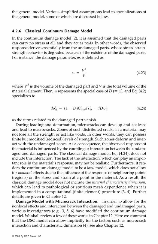
© 2001 By CRC Press LLC
the general model. Various simplified assumptions lead to specializations ofthe general model, some of which are discussed below.
4.2.6 Classical Continuum Damage Model
In the continuum damage model (2), it is assumed that the damaged partscan carry no stress at all, and they act as voids. In other words, the observedresponse derives essentially from the undamaged parts, whose stress–strain-strength behavior is degraded because of the existence of the damaged parts.For instance, the damage parameter, �, is defined as
(4.23)
where is the volume of the damaged part and V is the total volume of thematerial element. Then, � represents the special case of D (� �), and Eq. (4.2)specializes to
(4.24)
as the terms related to the damaged part vanish.During loading and deformation, microcracks can develop and coalesce
and lead to macrocracks. Zones of such distributed cracks in a material maynot lose all the strength or act like voids. In other words, they can possessfinite but modified (reduced) levels of strength. Such zones deform and inter-act with the undamaged zones. As a consequence, the observed response ofthe material is influenced by the coupling or interaction between the undam-aged and damaged parts. The classical damage model, Eq. (4.24), does notinclude this interaction. The lack of the interaction, which can play an impor-tant role in the material’s response, may not be realistic. Furthermore, it ren-ders the continuum damage model to be a local model, which does not allowfor nonlocal effects due to the influence of the response of neighboring points(regions) on the stress and strain at a point in the material. As a result, theclassical damage model does not include the internal characteristic dimension,which can lead to pathological or spurious mesh dependence when it isimplemented in a computational (finite-element) procedure (3, 4). Furtherdetails are given in Chapter 12.
Damage Model with Microcrack Interaction. In order to allow for thenonlocal effects and interaction between the damaged and undamaged parts,various investigators (e.g., 3, 5, 6) have modified the continuum damagemodel. We shall review a few of these works in Chapter 12. Here we commentthat the DSC model can allow implicitly for the factors such as microcrackinteraction and characteristic dimension (4); see also Chapter 12.
�Vd
V------�
Vd
d�ija 1 D�( )Cijk�
i d�k�i dD�ij
i��

© 2001 By CRC Press LLC
4.2.7 DSC Model Without Relative Motions
As stated earlier, the general DSC model can include different stresses andstrains in the RI and FA parts. Now, the incremental strain equations can bewritten as
(4.25)
where and show the functional dependence of total strains on thestrains in the RI and FA parts. If it is assumed that the observed, RI, and FAstrains are equal, that is, there is no relative motion between the RI and FAparts, we have
(4.26)
Then the behavior of the material can be characterized on the basis of onlythe stress equations, Eq. (4.2). The assumption of compatible strains, Eq.(4.26), can introduce an error; however, the stresses in the two parts can stillbe different [Eq. (4.2)].
FA Part—Constrained Liquid (Chapter 3). If it is assumed that the FApart can carry no shear stress but can carry hydrostatic stress Eq. (4.2) is sim-plified further. This assumption implies that the FA parts are constrained bythe surrounding RI parts and act like a constrained liquid. Then Eq. (4.2) spe-cializes to
(4.27)
An additional assumption that the hydrostatic stresses in the RI and FAparts are equal (i.e., � ) may sometimes be appropriate. Then Eq. (4.27)reduces to (7, 8)
(4.28)
In the following, we shall discuss the critical-state characterization of the FAbehavior. However, appropriate laboratory tests are not often available for allmaterials (other than geologic and concrete) to characterize and find parame-ters for the critical-state behavior. Hence, for practical applications, Eq. (4.28)may provide satisfactory characterization for some materials like metals, alloys,and ceramics. In this case, it is relatively easy to characterize the FA response
d�ija dEij
a 13---d�ii
a�ij��
f 1 dEiji , dEij
c( ) 13--- f 2 d�ii
i , d�iic( )�ij��
f 1 f 2
d�ija d�ij
i d�ijc
� �
d�ija 1 D�( )d�ij
i DdJ1
c
3-------�ij dD 1
3--- J1
c�ij Sij
i�
13--- J1
i�ij�
� ��
J1i J1
c
d�ija 1 D�( )d�ij
i DdJ1
i
3-------
�ij dDSiji
���

© 2001 By CRC Press LLC
corresponding to the second term in Eq. (4.28), which requires the (tangent)bulk modulus (K ) for the material in the FA state, if it were characterized as elas-tic, and relevant plasticity parameters if it were characterized as elastoplastic.
4.2.8 Critical-State Characterization for FA Response
As discussed in Chapter 3, an initially loose or dense (granular) materialwith a given initial mean pressure p0 � J10/3 approaches the critical state atwhich the material continues to experience shear strains under the constantshear stress reached up to that state. Thus, the material at the critical statecontinues to carry the specific shear stress for the given initial pressure andcan be considered to act like a constrained liquid–solid. This state can providea realistic simulation for the behavior of material at the FA state. It may benoted, however, that the use of the critical-state to represent the FA state inthe DSC involves different considerations than those in the classical critical-state concept in soil mechanics (9). In the latter, the main attention has beentoward the characterization of the final critical (collapse or failure) behaviorof soils (clays). In the DSC, on the other hand, the FA material consideredto be at the critical state can exist and grow, at distributed locations, fromthe very beginning of the loading. Only in the limiting case does the entirematerial element approach the critical state.
The behavior of material at the critical state is characterized based on the fol-lowing two equations (see also Chapter 3):
(4.29a)
(4.29b)
where and are the invariants at the critical state (here, J1�3 is non-dimensionalized with respect to pa), is the slope of the vs. line[Fig 3.3(d), Chapter 3], is the initial value of the critical void ratio, , cor-responding to � 3pa, pa is the atmospheric pressure constant, and � is theslope of the e vs. �n ( /3pa) line (Fig. 3.3(e)). in Eq. (4.2) can now beobtained by using Eq. (4.29), as described below.
4.2.9 DSC Equations with Critical State
Consider the stress and incremental stress relations in Eq. (4.1). The observedstress is now expressed as the sum of the shear and isotropic components as
(4.30a)
J2Dc mJ1
c�
ec e0c
��n J1c�3pa( )��
J2Dc J1
c
m J1c J2D
c
e0c ec
J1c
J1c Cijk�
c
Sija 1
3--- J1
a�ij� 1 D�( ) Sij
i 13--- J1
i�ij�
D Sijc 1
3--- J1
c�ij�
��

© 2001 By CRC Press LLC
If we assume that � � � J1, Eq. (4.30a) reduces to
(4.30b)
Now, as a simplification, assume the following relation between the shearstresses:
(4.31a)
which with the relation 1�2SijSij � J2D leads to
(4.31b)
Now, from Eq. (4.29a), we derive
(4.32)
where � � / .Therefore,
(4.33)
Now
(4.34a)
Hence, from Eqs. (4.30b) and (4.32), we have
(4.34b)
(4.34c)
Differentiation of Eq. (4.34c) leads to
(4.35a)
J1a J1
i J1c
Sija 1 D�( )Sij
i DSijc
��
Sija F1 D( )Sij
i F2 D( )Sijc
� �
J2Di F2
F1----- J2D
c�
Sijc mJ1
c
J2Di
-----------Siji mJ1
i
J2Di
----------- Siji m�Sij
i� � �
J1i J2D
i
�ijc m�( )Sij
i 13--- J1
i�ij��
�ija Sij
a 13--- J1
a�ij��
�ija 1 D�( )Sij
i DSijc 1
3--- J1
i�ij� ��
1 D�( )Siji Dm�Sij
i 13--- J1
i�ij
i���
d�ija 1 D�( )dSij
i� dDSij
i Dm�dSiji
��
DmSiji d� m�Sij
i dD 13---dJ1
i�ij� � �

© 2001 By CRC Press LLC
or
(4.35b)
Finally,
(4.35c)
in which
(4.36a)
and
(4.36b)
where Kt is the (tangent) bulk modulus. Equation (4.35c) expresses theobserved stress increment in terms of the RI stresses, and stress and strainincrements, the critical-state parameter ( ), and the stress ratio, �. Itinvolves the assumption that the mean pressures in the observed, RI, and FAparts are equal, which can be appropriate for many situations. Note that if
� 0, that is, the FA part cannot carry any shear stress, Eq. (4.35c) willreduce to Eq. (4.28).
Furthermore, as will be discussed later (Chapter 13), Eq. (4.35) leads to thecomputation of observed stress increments, , and the RI strain increments,
. Then we need to evaluate the observed strain increment, correspond-ing to . Often it is possible to make the additional assumption that the total(or deviatoric or hydrostatic) strains are equal in the three parts, that is,
� � . This assumption can be considered to be similar to compat-ibility of strains (no diffusion) in the components of a porous multiphasematerial (10), implying that there are no relative motions between the RI andFA parts. With this assumption of compatible strains, the DSC formulationwould require use of only the stress equations (4.35), and its implementationin the computer procedures would be simplified.
d�ija Dm� 1 D�( )�[ ]dSij
i Dm� 1 D�( )�[ ]dJ1
i
3-------�ij��
Dm� 1 D�( )�[ ]dJ1
i
3-------�ij DmSij
i d���
dD m�Siji Sij
i�( ) 1
3---dJ1
i�ij� �
d�ija Dm� 1 D�( )�[ ]d�ij
i D Dm��( )dJ1
i
3-------�ij��
dD m� 1�( ) Dmd��[ ]Siji
�
d�iji Cijk�
i d�k�i
�
dJ1i
3------- Ktd�v
i�
m
m
d�ija
d�iji d�ij
a
d�ija
d�ija d�ij
i d�ijc
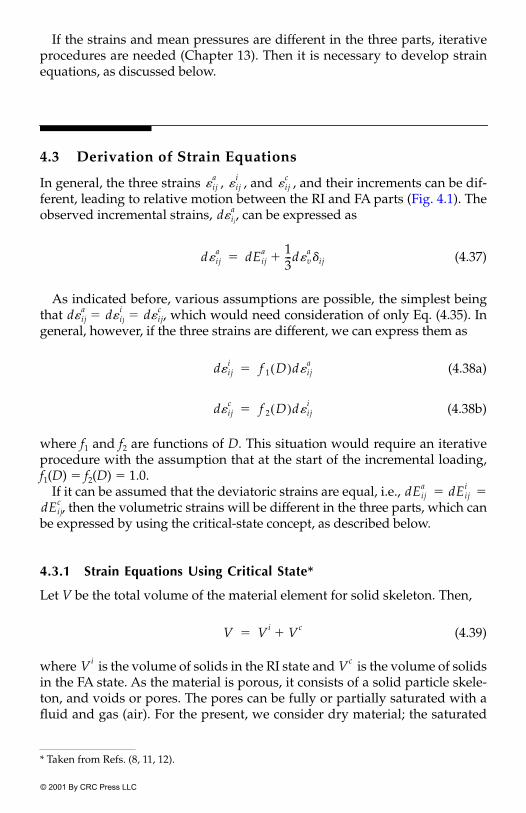
© 2001 By CRC Press LLC
If the strains and mean pressures are different in the three parts, iterativeprocedures are needed (Chapter 13). Then it is necessary to develop strainequations, as discussed below.
4.3 Derivation of Strain Equations
In general, the three strains , , and , and their increments can be dif-ferent, leading to relative motion between the RI and FA parts (Fig. 4.1). Theobserved incremental strains, , can be expressed as
(4.37)
As indicated before, various assumptions are possible, the simplest beingthat � � , which would need consideration of only Eq. (4.35). Ingeneral, however, if the three strains are different, we can express them as
(4.38a)
(4.38b)
where f1 and f2 are functions of D. This situation would require an iterativeprocedure with the assumption that at the start of the incremental loading,f1(D) � f2(D) � 1.0.
If it can be assumed that the deviatoric strains are equal, i.e., � �, then the volumetric strains will be different in the three parts, which can
be expressed by using the critical-state concept, as described below.
4.3.1 Strain Equations Using Critical State*
Let V be the total volume of the material element for solid skeleton. Then,
(4.39)
where is the volume of solids in the RI state and is the volume of solidsin the FA state. As the material is porous, it consists of a solid particle skele-ton, and voids or pores. The pores can be fully or partially saturated with afluid and gas (air). For the present, we consider dry material; the saturated
* Taken from Refs. (8, 11, 12).
�ija
�iji
�ijc
d�ija
d�ija dEij
a 13---d�v
a�ij��
d�ija d�ij
i d�ijc
d�iji f 1 D( )d�ij
a�
d�ijc f 2 D( )d�ij
i�
dEija dEij
i
dEijc
V Vi Vc��
Vi Vc

© 2001 By CRC Press LLC
condition will be treated later in Chapter 9. As a result, we deal with effectivestresses.
We decompose the volume of solids, Vs, and the volume of voids, Vv , asfollows:
(4.40)
(4.40b)
where the superscripts i and c denote volumes in the RI and FA states, respec-tively. In the case of porous materials, the void ratio (e) is defined to denotethe ratio of the volume of voids (Vv) to that of solids (Vs) (13). Hence,
(4.41a)
or
(4.41b)
Now let the disturbance based on the volume of solids at critical state to the total volume of solids (Vs) be given by
(4.42a)
hence,
(4.42b
Therefore,
(4.42c)
where � is the void ratio of the RI part and � is the voidratio of the FA parts.
Differentiation of in Eq. (4.42c) gives (here, the subscript e on D isdropped for convenience)
(4.43)
Vs Vsi Vs
c��
Vv Vvi Vv
c��
ea Vv
Vs------
Vvi Vv
c�
Vs---------------------
Vvi Vs
i
Vs Vsi
-----------------
Vvc Vs
c
Vs Vsc
-----------------�� � �
ea Vvi
Vsi
------Vs Vs
c�
Vs--------------------
Vvc Vs
c
Vsc Vs
-----------------��
Vsc( )
De
Vsc
Vs------�
Vsi�Vs 1 De��
ea 1 De�( )ei Deec
��
ei Vvi Vs
i� ec Vv
c�Vs
c
ea
dea 1 D�( )dei Ddec dD ec ei�( )� ��

© 2001 By CRC Press LLC
The relation between incremental volume (d�v) and the void ratio (de) isgiven by (9, 13, 14)
(4.44)
where e0 is the initial void ratio. Then Eq. (4.43) becomes
(4.45)
The observed strain, , can be written as
(4.46)
Now, from Eq. (4.29b), the void ratio can be expressed as
(4.29b)
Therefore,
(4.47a)
and
(4.47b)
Then Eq. (4.46) leads to
(4.48)
d�vde
1 e0�---------------��
d�va 1 D�( )d�v
i Dd�vc dD ei ec
�1 e0�---------------
���
d�ija
d�ija dEa
ij13---d�v
a�ij��
dEaij
13---�ij 1 D�( )d�v
i Dd�vc dD ei ec
�1 e0�---------------
����
ec
ec e0c
��n J1c�3pa( )��
dec�
dJ1c
J1c
-------��
d�va �
1 e0�---------------
dJ1c
J1c
-------��
d�ija dEij
a 13---�ij 1 D�( )d�v
i D�
1 e0�---------------�
dJ1c
J1c
-------���
d� Dei e0
c� ��n J1
c�3pa( )�
1 e0�------------------------------------------------------

© 2001 By CRC Press LLC
Hence, with the FA state simulated by using the critical-state equations, thesolution should lead to (approximate) simultaneous satisfaction of the stress,Eq. (4.35), and strain, Eq. (4.48), during the iterative procedures described inthe following and in Chapter 13.
The foregoing simulation for the FA material by using the critical-stateequations, Eq. (4.29), is used for geologic (soils and rocks) materials and con-crete, because volumetric (void ratio) measurements are often availabletogether with the stress–strain response. For materials such as metals andalloys, volumetric measurements are usually not available. Hence, the use ofthe critical-state equations may not be feasible. In such cases, the alternativesimulation for the FA state as a constrained liquid that can carry mean stressbut no shear stress ( � 0.0) can be used [Eq. (4.28)].
4.4 General Formulation of DSC Equations
The assumptions of compatible strains and mean pressures in the three stateslead to simplified equations only in terms of observed stress increment. How-ever, in general, the strains and mean pressure can be different, and itbecomes necessary to obtain convergent solutions based on both the stressand strain equations, Eqs. (4.2) and (4.48). In the following, we discuss sucha general procedure.
The functions f1 and f2 in Eq. (4.38) may be assumed to be scalars �2 and �1,which can vary during the incremental iterative procedure (15):
(4.49a)
(4.49b)
Now Eq. (4.2) can be expressed in matrix notation as
(4.50a)
where dD � [Eq. (4.14b)]. Substitution of Eq. (4.49) into Eq. (4.50a) leadsto
(4.50b)
where
m
d� ijc
�1d� iji or d�
˜c
�1d� i� �
d� iji
�2d� ija or d�
˜i
�2d�˜
a� �
d�˜
a 1 D�( )C˜
id�˜
i DC˜
cd�˜
c R˜
T�˜
c�˜
i�( )d�
˜i
� ��
R˜
Td�˜
i
d�˜
a 1 D�( )�2C˜
i�1�2DC
˜c
�2R˜
T�˜
c�˜
i�( )� �[ ]d�
˜a
�
L˜ nd�n
a�
L˜ n 1 D�( )�2C
˜i
�1�2DC˜
c�2R
˜T
�˜
c�˜
i�( )� ��
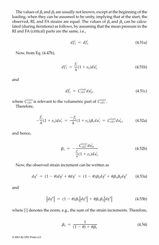
© 2001 By CRC Press LLC
The values of �1 and �2 are usually not known, except at the beginning of theloading, when they can be assumed to be unity, implying that at the start, theobserved, RI, and FA strains are equal. The values of �1 and �2 can be calcu-lated (during iterations) as follows, by assuming that the mean pressure in theRI and FA (critical) parts are the same, i.e.,
(4.51a)
Now, from Eq. (4.47b),
(4.51b)
and
(4.51c)
where is relevant to the volumetric part of .Therefore,
(4.52a)
and hence,
(4.52b)
Now, the observed strain increment can be written as
(4.53a)
and
(4.53b)
where � � denotes the norm, e.g., the sum of the strain increments. Therefore,
(4.54)
dJ1c dJ1
i�
dJ1c J1
c
�---- 1 e0�( )d�v
c�
dJ1i Ciik�
i ep( )d�k�i
�
Ciik�i ep( ) Cijk�
i ep( )
J1c
�---- 1 e0�( )d�v
c�
J� 1c
�--------- 1 e0�( )�1d�v
i Ciik�i ep( )d�k�
i� �
�1
Ciik�i ep( )d�k�
i
J1c
�---- 1 e0�( )d�v
i
---------------------------------��
d�˜
a 1 ��( )d�˜
i�d�
˜c
� 1 ��( )�2d�˜
a��1�2d�
˜a
�� �
d�˜
a 1 ��( )�2 d�˜
a��1�2 d�
˜a
��
�21
1 ��( ) ��1�------------------------------------�

© 2001 By CRC Press LLC
Here �, the interpolation factor (0 � � � 1), can be assumed to be the distur-bance, D (0 � D � 1), which varies during the incremental-iterative analysis.
4.5 Alternative Formulations of DSC
Consider a material element composed of two materials, 1 and 2 [Eq. (2.8),Chapter 2]. Elements of each material can involve RI and FA states during itsdeformation. The incremental equation for materials 1 and 2 can be expressed as
(4.55a)
and
(4.55b)
Then the observed incremental response of the composite element can bewritten as
(4.56)
For a material element composed of solids and fluid, the incremental formof Eq. (2.14b) is derived as
(4.57a)
For bonded materials, e.g., Eq. (2.30a), the incremental equations are given by
(4.57b)
4.6 Examples
Example 4.1Consider the uniaxial stress–strain behavior, shown in Fig. 4.2. Assume theRI behavior to be (a) linear elastic and (b) nonlinear elastic simulated by ahyperbola. Assume the FA stress state as � 17 N/ . Also assume thatthe disturbance, D [Eq. (4.13a)], is expressed only in terms of the axial totalstrain (�) or plastic strain ( ).
d�1ija 1 D1�( )Cijk�
1i d�k�1i D1Cijk�
1c d�k�1c dD1 �ij
1c�ij
1i�( )� ��
d�2ija 1 D2�( )Cijk�
2i d�k�2i DCijk�
2c d�k�2c dD2 �ij
2c�ij
2c�( )� ��
d�ija 1 D�( )d�1ij
a Dd�2ija dD �ij
2a�ij
1a�( )� ��
d�ija 1 D�( )dp f
�ij Dd�ijs dD �ij
s p f�ij�( )� ��
d�ija 1 D�( )Cijk�
i d�k�i DCijk�
b d�k�b dD �ij
b�ij
i�( )� ��
�c mm2
�p
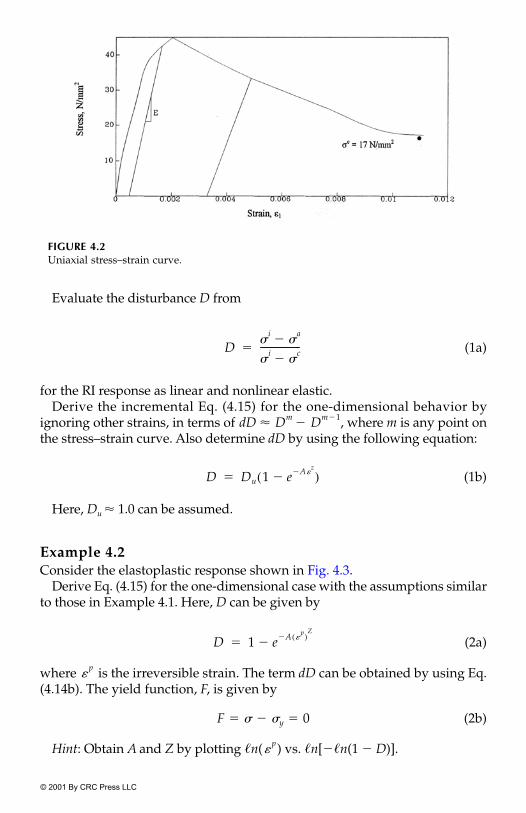
© 2001 By CRC Press LLC
Evaluate the disturbance D from
(1a)
for the RI response as linear and nonlinear elastic.Derive the incremental Eq. (4.15) for the one-dimensional behavior by
ignoring other strains, in terms of dD � � , where m is any point onthe stress–strain curve. Also determine dD by using the following equation:
(1b)
Here, Du � 1.0 can be assumed.
Example 4.2Consider the elastoplastic response shown in Fig. 4.3.
Derive Eq. (4.15) for the one-dimensional case with the assumptions similarto those in Example 4.1. Here, D can be given by
(2a)
where is the irreversible strain. The term dD can be obtained by using Eq.(4.14b). The yield function, F, is given by
F � � � �y � 0 (2b)
Hint: Obtain A and Z by plotting �n( ) vs. �n[��n(1 � D)].
FIGURE 4.2Uniaxial stress–strain curve.
D�
i�
a�
�i
�c
�------------------�
Dm Dm�1
D Du 1 e A�z
��( )�
D 1 e A �p( )
Z�
��
�p
�p

© 2001 By CRC Press LLC
Example 4.3Derive Eq. (4.15) for the one-dimensional case in Example 4.2 by using thevon Mises criterion:
(3a)
Example 4.4Consider the lateral strains, �2 � �3, for the uniaxial stress behavior. Let begiven by
(4a)
and
(4b)
Derive Eq. (4.15) by using the von Mises criterion.
References
1. Desai, C.S., Chia, J., Kundu, T., and Prince, J., “Thermomechanical Responseof Materials and Interfaces in Electronic Packaging, Part I—Unified Constitu-tive Model and Calibration; Part II—Unified Constitutive Model, Validationand Design,” J. of Electronic Packaging, ASME, 119, 4, 1997, 294–300; 301–309.
2. Kachanov, L.M., Introduction to Continuum Damage Mechanics, Martinus NijhoftPublishers, Dordrecht, The Netherlands, 1986.
FIGURE 4.3Elastoplastic response.
F J2D k� 0� �
d�12 2d�2
2�( )1�2��
D 1 e AZ
���

© 2001 By CRC Press LLC
3. Bazant, Z.P. and Cedolin, L., Stability of Structures, Oxford Univ. Press, NewYork, 1991.
4. Desai, C.S., Basaran, C., and Zhang, W., “Numerical Algorithms and MeshDependence in the Disturbed State Concept,” Int. J. Num. Meth. Eng., 40, 1997,3059–3083.
5. Bazant, Z.P., “Nonlocal Damage Theory Based on Micromechanics of CrackInteractions,” J. of Eng. Mech., ASCE, 120, 1994, 593–617.
6. Mühlhaus, H.B., Continuum Models for Materials with Microstructure, John Wiley& Sons, UK, 1995.
7. Frantziskonis, G. and Desai, C.S., “Constitutive Model with Strain Softening,”Int. J. Solids & Struct., 23, 6, 1987, 751–767.
8. Desai, C.S., “Constitutive Modelling Using the Disturbed State as Microstruc-ture Self-Adjustment Approach,” Chap. 8 in Continuum Models for Materialswith Microstructure, John Wiley & Sons, Chichester, UK, 1995.
9. Schofield, A.N. and Wroth, C.P., Critical State Soil Mechanics, McGraw-Hill,London, 1968.
10. Bowen, R.M., “Theory of Mixtures” in Continuum Physics, Eringen, A.C. (Editor),Academic Press, New York, 1976.
11. Armaleh, S.H. and Desai, C.S., “Modelling and Testing of a Cohesionless SoilUsing the Disturbed State Concept,” Int. J. Mech. Behavior of Materials, 5, 3, 1994.
12. Katti, D.R. and Desai, C.S., “Modelling and Testing of Cohesive Soils Using theDisturbed State Concept,” J. of Eng. Mech., ASCE, 121, 5, 1995, 648–658.
13. Terzaghi, K., Peck, R.B., and Mesri, G., Soil Mechanics in Engineering Practice,John Wiley & Sons, New York, 1996.
14. Desai, C.S. and Siriwardane, H.J., Constitutive Laws for Engineering Materials,Prentice-Hall, Englewood Cliffs, NJ, 1984.
15. Shao, C. and Desai, C.S., “Implementation of DSC Model for Dynamic Analysisof Soil-Structure Interaction Problems,” Report to NSF, Dept. of Civil Engng.and Engng. Mechanics., University of Arizona, Tucson, AZ, USA, 1998.

© 2001 By CRC Press LLC
5Theory of Elasticity in DSC
CONTENTS5.1 Linear Elasticity
5.1.1 Nonlinear or Piecewise Linear Behavior5.2 Variable Parameter Models
5.2.1 Functional Forms5.2.2 Hyperelastic Models5.2.3 First-Order Model5.2.4 Second-Order Cauchy Elastic Model
5.3 Relatively Intact Behavior5.4 Fully Adjusted Behavior5.5 Disturbance Function5.6 Material Parameters
5.6.1 Thermal Effects: Thermoelasticity5.7 Examples
5.7.1 Correlation with Crack Density
As derived in Chapter 2, the DSC equations are given by
(5.1)
In this chapter, we present the theory of elasticity as the model for thebehavior of the material in the RI state, represented by the constitutive tensor,
.
5.1 Linear Elasticity
If the behavior of the RI material is characterized as linear elastic with theassumption of isotropy, the constitutive equations will be given by (1–3)
(5.2a)
d�ija 1 D�( )Cijk�
i d�k�i DCijk�
c d�k�c dD �ij
c�ij
i�( )� ��
Cijk�i
�iji Cijk�
i e( )�k�
i�

© 2001 By CRC Press LLC
or
(5.2b)
where is the stress tensor for the RI material
(5.3)
and is the strain tensor
(5.4)
where �11, �22, �33 and �11, �22, �33 are the normal, and �12, �23, �13 and �12, �23,�13 the shear components of stress and strain, respectively. and are thevectors of stress and strain components, given by
(5.5)
The fourth-order constitutive tensor, , for linear elastic and isotropicmaterials can be expressed in matrix notation using the generalized Hooke’slaw as (4)
(5.6)
�˜
i C˜
i e( )�˜
i�
�iji
�iji
�11 �12 �13
�12 �22 �23
�13 �23 �33
i
�
�iji
�iji
�11 �12 �13
�12 �22 �23
�13 �23 �33
i
�
�˜
i�˜
i
�˜
i
�11
�22
�33
�12
�23
�13
; �˜
i
�11
�22
�33
�12
�23
�13
� �
Cijk�i e( )
�11
�22
�33
�12
�23
�13
i
E1 ��( ) 1 2��( )
-----------------------------------------
1 �� � � 0 0 0 1 �� � 0 0 0 1 �� 0 0 0 1 2�� 0 0
symmetrical 1 2�� 0 1 2��
i �11
�22
�33
�12
�23
�13
�

© 2001 By CRC Press LLC
Here, 2�12 � �xy, 2�23 � �yz, and 2�13 � �xz, where �xy ,�yz, and �xz are engineer-ing shear strains, E is the elastic modulus, and ν is the Poisson’s ratio.
In terms of the shear modulus, G, and the bulk modulus, K, Eq. (5.6)becomes
(5.7)
The relations between the elastic constants are given by
(5.8a)
(5.8b)
5.1.1 Nonlinear or Piecewise Linear Behavior
Note that the material parameters E and �, K and G are evaluated as tan-gent quantities when Hooke’s law, Eq. (5.2), is written in the incrementalform
(5.9)
where the subscript t denotes tangent quantity. In this case, the nonlinearresponse (see Fig. 5.1)is approximated as piecewise linear by dividing thenonlinear behavior in a number of linear increments. The material parame-ters are often assumed to be constant within each increment. The monotonicresponse of some nonlinear materials is often simulated by using the piece-wise linear approximation in which the parameters or moduli (Et, νt, Gt, Kt)vary from increment to increment. Such models are often referred to as quasi-linear or variable parameter or variable moduli (4).
�11
�22
�33
�12
�23
�13
i K4G3
-------� K2G3
-------�K 2G�
3------------------- 0 0 0
K4G3
-------� K2G3
-------� 0 0 0
K4G3
-------� 0 0 0
2G 0 0 2G 0 2G
i
�11
�22
�33
�12
�23
�13
i
�
GE
2 1 ��( )----------------------�
KE
3 1 2��( )-------------------------�
d�˜
i C˜ t
i e( )d�˜
i�

© 2001 By CRC Press LLC
5.2 Variable Parameter Models
Here, the nonlinear behavior expressed as a stress–strain response can besimulated using mathematical functions. Then, the tangent moduli are eval-uated as derivatives of the function at (selected) points in an increment. Someof the commonly used functions are stated below.
5.2.1 Functional Forms
Observed nonlinear stress–strain data can be simulated by using mathemat-ical functions such as polynomials, hyperbola, spline, and exponential (4).For example, schematics of such stress–strain curves for different initial meanpressure (�0) and density (�0) are shown in Fig. 5.2; here the stress–strainresponses are expressed in terms of stress measure, which can be axialstress (�1), stress difference (�1 � �3), octahedral shear stress, oct, or secondinvariant of the deviatoric stress tensor, Sij, given by
(5.10a)
where Sij � � ij � (13)�ii�ij, �ii � J1 � first invariant of �ij, �ij � Kronecker delta,�i (i � 1, 2, 3) � principal stresses, and
(5.10b)
FIGURE 5.1Piecewise linear approximation to nonlinear behavior.
�,
J2D( )
J2D16--- �1 �2�( )2
�2 �3�( )2�1 �3�( )2
� �[ ]�
oct2 2
3--- J2D�

© 2001 By CRC Press LLC
The strain measure, in Fig. 5.2, can be the axial strain, �1, strain difference�1 � �3, octahedral shear strain, �oct, or the second invariant (I2D) of the devi-atoric strain tensor, Eij:
(5.10c)
(5.11a)
(5.11b)
where I1 is the first invariant of the total strain tensor, �ij, �i (i � 1, 2, 3) are theprincipal strains, and
(5.11c)
As is indicated in Fig. 5.2, the stress–strain behavior depends on factors suchas (initial) mean pressure, p0 or �0, and density (�0). Hence, for a given valueof �0, the functional form of the stress–strain relation can be expressed as
(5.12a)
and for the behavior dependent on �0
(5.12b)
FIGURE 5.2Functional representation of nonliner stress–strain response.
�
I2D16--- �1 �2�( )2
�2 �3�( )2�1 �3�( )2
� �[ ]�
Eij �ij13---�ii�ij��
�ii �v I1� �
�oct2 2
3---I2D�
� � �( )�
� � �,�0( )�

© 2001 By CRC Press LLC
or
Then, the tangent moduli such as Et (Young’s elastic), vt (Poisson’s ratio), Gt
(shear modulus), and Kt (bulk modulus) can be obtained as appropriatederivatives of the function in Eq. (5.12). For example:
(5.13a)
(5.13b)
(5.13c)
(5.13d)
The above quasilinear elastic models are based on the idea that the nonlin-ear response can be simulated incrementally based on the variable values ofthe tangent material moduli as functions of stress and/or strain. The nonlin-ear behavior can be simulated more formally by using higher-order or hyper-elastic and hypoelastic models; the above quasilinear models can be shownto be special (lowest) cases of the higher-order models (4).
5.2.2 Hyperelastic Models
Cauchy and Green elastic are two of the main models often used to charac-terize the nonlinear elastic behavior of materials. Details of these models aregiven in various publications (1, 4–6). Here we give a brief description of theCauchy elastic models, in which the relation between stress and strain isexpressed as
(5.14a)
where �0, �1,…, �n represent response functions or parameters. By using theCayley–Hamilton theorem (7), we can write Eq. (5.14a) as
(5.14b)
� � �,p0 or J10 3( )�
Et
d �1 �3�( )d�1
---------------------------�0 constant�
�
�t
d�3
d�1--------
�0 constant�
��
Kt
d J13( )d�v
------------------�
Gt
d oct( )d �oct( )----------------�
�ij �0�ij �1�ij �2�im�mj �3�im�mn�nj…� � � ��
�ij 0�ij 1�ij 2�im�mj� ��

© 2001 By CRC Press LLC
where 0, 1, and 2 are the response functions expressed in terms of theinvariants I1, I2, and I3 of the strain tensor. We can derive various special formsof Eq. (5.14) with different orders, some of which are described below.
5.2.3 First-Order Model
For the first-order model, only the first two terms in Eq. (5.14b) are relevant,and 2 � 0. Then 1 is a constant (say, � �2), and 0 can be a linear functionof the first strain invariant, say (� �0�ij � �1I1�ij), and Eq. (5.14) becomes
(5.15a)
In this equation, �0�ij is the initial (isotropic) stress when the strain � 0.Hence, if we start from a stressfree condition, Eq. (5.15a) reduces to
(5.15b)
where �1 and �2 are elastic material constants. It can be shown that the first-order Cauchy elastic model, Eq. (5.15b), is the same as linear elastic Hooke’slaw for isotropic materials. This can be done as follows:
Let us first consider the state of uniform volumetric deformation. Then thestrain tensor, �ij, is given by
(5.16a)
Substitution of Eq. (5.16a) in Eq. (5.15) gives
(5.16b)
For isotropic or hydrostatic stress condition, the mean pressure, p, is given by
(5.17a)
Therefore, Eq. (5.16b) becomes
(5.17b)
where K is the bulk modulus; see Fig. 5.3(a).
�ij �0�ij �1I1�ij �2�ij� ��
�ij �1I1�ij �2�ij��
�ijI1
3----
�ij
I13 0 00 I13 00 0 I13
� �
�ij �1I1 �2I1
3----�
�ij�
p�ij
3------
J1
3----
�11 �22 �33� �
3--------------------------------------� � �
J1
3---- �1
�2
3-----�
I1 KI1� �

© 2001 By CRC Press LLC
Now we consider the case of pure shear strain condition, which impliesthat for an isotropic material, there is no volumetric strain and there existonly nonzero shear strain components, �12 � �21. Then Eq. (5.15b) becomes
(5.18a)
or
(5.18b)
Here, �12 �1/2 �12, where �12 is the engineering shear strain. Then, from Eq.(5.18), we have
(5.19a)
FIGURE 5.3Bulk and shear moduli.
�ij �2�ij�
�ij
0 �2�12 0�2�12 0 0
0 0 0
�
�12 �2�12
2-------
�

© 2001 By CRC Press LLC
Therefore,
(5.19b)
where G � �2/2 is the shear modulus; see Fig. 5.3(b).Now, substitution of �2 � 2G in Eq. (5.17b) leads to
(5.20)
and
(5.21a)
(5.21b)
With the above values of �1 and �2, Eq. (5.15b) is written as
(5.22)
Note that the strain tensor, �ij, can be decomposed as
(5.23)
where Eij is the deviatoric strain tensor. Then, Eq. (5.22) can be expressed as
(5.24)
where Sij is the deviatoric stress tensor and J1/3 is the mean pressure. Notethat Eq. (5.24) represents the generalized Hooke’s law for linear elastic behav-ior, from Eq. (5.2).
�12
�2
2-----�12 G�12� �
J1
3---- �1
2G3
-------� I1�
K �12G3
-------��
�1 K2G3
-------��
�ij K2G3
-------� I1�ij 2G�ij��
� KI1�ij 2G �ijIi
3---�ij�
�
�ij EijI1
3----�ij��
�ij KI1�ij 2GEij��
�J1
3----�ij Sij�
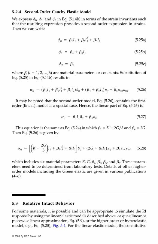
© 2001 By CRC Press LLC
5.2.4 Second-Order Cauchy Elastic Model
We express 0, 1, and 2 in Eq. (5.14b) in terms of the strain invariants suchthat the resulting expression provides a second-order expression in strains.Then we can write
(5.25a)
(5.25b)
(5.25c)
where �i (i � 1, 2,…,6) are material parameters or constants. Substitution ofEq. (5.25) in Eq. (5.14b) results in
(5.26)
It may be noted that the second-order model, Eq. (5.26), contains the first-order (linear) model as a special case. Hence, the linear part of Eq. (5.26) is
(5.27)
This equation is the same as Eq. (5.24) in which �1 � K � 2G/3 and �4 � 2G.Then Eq. (5.26) is given by
(5.28)
which includes six material parameters K, G, �2, �3, �5, and �6. These param-eters need to be determined from laboratory tests. Details of other higher-order models including the Green elastic are given in various publications(4–6).
5.3 Relative Intact Behavior
For some materials, it is possible and can be appropriate to simulate the RIresponse by using the linear elastic models described above, or quasilinear orpiecewise linear approximation, Eq. (5.9), or the higher-order or hyperelasticmodel, e.g., Eq. (5.28), Fig. 5.4. For the linear elastic model, the constitutive
0 �1I1 �2I12
�3I2� ��
1 �4 �5I1��
2 �6�
�ij �1I1 �2I12
�3I2� �( )�ij �4 �5I1�( )�ij �6�im�mj� ��
�ij �1I1�ij �4� �ij�
�ij K2G3
-------� I1 �2I1
2�3I2� � �ij 2G �5I1�( )�ij �6�im�mj� ��

© 2001 By CRC Press LLC
tensor for the RI material, Eq. (5.2), can be written as
(5.29)
For the quasilinear and (incremental) hyperelastic model, it can be written as
(5.30)
where the subscript t denotes tangent modulus, which is evaluated as thederivative or slope (at a point) based on the function used to simulate thebehavior.
If there is no disturbance due to microcracking, damage, softening, or stiff-ening, D in Eq. (5.1) will be zero, and the observed (denoted by a) and RIresponses will be the same. However, if a linear or nonlinear elastic materialexperiences disturbance, the observed behavior, Fig. 5.4, will deviate fromthe behavior without the disturbance, i.e., the RI response.
5.4 Fully Adjusted Behavior
If the material experiences microcracks and disturbance (damage), and if thecracked zones are assumed to behave like voids, as in the classical damage mod-els (8), then such FA or damaged zones will have zero strength (Chapter 3).Hence, they can carry no stress, and the corresponding constitutive matrix inEq. (5.1) will be
(5.31a)
It may be realistic to assign a finite (small) elastic stiffness to the disturbed,cracked, or damaged regions. Then,
(5.31b)
FIGURE 5.4Elastic model as RI characterization.
Cijk�i
Cijk�i e( ) Cijk�
e K, G, or E, �( )�
Cijk�i e( ) Cijk�
e Kt, Gt; Et, �t( )�
C˜
c 0˜
�
C˜
c C˜
c Ktc, Gt
c; Etc, �t
c( )�

© 2001 By CRC Press LLC
where the superscript c denotes the FA state, etc. are (tangent) elasticparameters with modified (reduced) values corresponding to the zone instress–strain response relevant to the FA state; see Fig. 5.4.
If it is assumed that the FA material can carry hydrostatic stress and noshear stress, assuming that the bulk behavior of the FA material is the sameas that of the RI material, the constitutive matrix can be expressed as [seeEq. (4.19a), Chapter 4]
(5.32a)
Now from Eq. (5.7), we can obtain
(5.32b)
or
Thus, the behavior of the FA material may be defined based on the bulkmodulus, of the RI material. The bulk modulus can also be defined as Kc,determined from the moduli ( or ) in the residual region of thestress–strain response (Fig. 5.4).
5.5 Disturbance Function
Based on available stress–strain data (Fig. 5.4), the disturbance function, D,can be expressed (approximately) as (Chapter 3)
(5.33)
Then, Eq. (5.1) can be used to obtain one-, two-, and three-dimensional ide-alizations. For example, for the uniaxial case (�22 � �33 � 0.0) and isotropicmaterial, Eq. (5.1) reduces to
(5.34)
and for the plane-stress case
(5.35)
Ktc, Gt
c,
C˜
cC˜
i�
�11 �22 �33� �( )i 3Ki�11 �22 �33� �( )i
�
Ki J1i
3�vi
--------�
Ki,Ec Gc
D�
�i
�a
�
�i
�c
�------------------�
d�11a 1 D�( )Eid�11
i DEcd�11c dD �11
c�11
i�( )� ��
d�˜
a 1 D�( )C˜
id�˜
i DC˜
cd�˜
c dD �˜
c�˜
i�( )� ��

© 2001 By CRC Press LLC
where
5.6 Material Parameters
For linear elastic behavior, the material parameters are E, ν, G, and K. In general,for nonlinear behavior, these parameters are obtained as (average) slopes of theunloading response. The elastic Young’s modulus, E, can be obtained fromuniaxial stress (�1 vs. �1) or triaxial tests (�1 or �1 � �3) vs. �1 (�3 � constant)plots; see Fig. 5.5(a). Poisson’s ratio can be obtained from the lateral strain (�3)or volumetric strains vs. �1 plots, shown in Fig. 5.5(b). The shear modulus, G, isobtained from shear tests as the unloading slope of shear stress ( or ) vs.shear strain (� or ) plots; see Fig. 5.5(c). The bulk modulus is obtained fromvolumetric or hydrostatic tests as the unloading slope of mean pressure (p orJ1/3) vs. volumetric strain (�v) plots; see Fig. 5.5(d).
5.6.1 Thermal Effects: Thermoelasticity
The temperature effects on the elastic response can be introduced by express-ing the parameters, say, E and ν or K and G, as functions of temperature andby modifying the elasticity equations to allow for the effect of the thermalexpansion. Then, Eq. (5.2) can be written as
(5.36)
where T is the temperature, �T is the coefficient of thermal expansion, dT isthe change in temperature, �ij is the Kronecker delta, and is the tem-perature-dependent constitutive tensor.
The material constants are determined from laboratory stress–strain testsat different temperatures and are expressed in terms of the temperature. Anumber of functional forms are possible and used in the literature (9–11).The following form has often been used and can simulate the temperature-dependent response of many materials (12):
(5.37)
d�˜
T d�11 d�22 d�12[ ]�
�˜
iT�11 �22 �12[ ]i
�
�˜
cT�11 �22 �12[ ]c
�
C˜
Et
1 �t2
�----------------
1 �t 0 1 0
symm 1 �t�
�
J2D
I2D
d�iji Cijk�
i e( ) T( ) d�k� �T T( )dT�k��[ ]�
Cijk�i e( ) T( )
p T( ) prTTr-----
c
�

© 2001 By CRC Press LLC
where Tr is the reference temperature (e.g., 300 K), pr is the value of theparameter at temperature Tr , and c is a parameter found from laboratorytests. For example, based on available laboratory tests at different tempera-tures for 60/40 (Sn/Pb) solders (13–15), plots of variations of E, �, and �T
were obtained; see Fig. 5.6 (16). Then the thermal dependence of these param-eters is expressed as
(5.38a)
(5.38b)
(5.38c)
where E300 � 23.45 GPa, ν300 � 0.40, and �T(300) � 3 � 10�6/K.
FIGURE 5.5Elastic constants from laboratory test data.
E T( ) 23.45 T300---------
0.292�
�
� T( ) 0.40 T300---------
0.14
�
�T T( ) 3�10 6� T300---------
0.24
�

© 2001 By CRC Press LLC
5.7 Examples
Example 5.1Consider the one-dimensional specialization of the DSC equations (Eq. 5.1) as
(1a)
where �1 and �1 are uniaxial stress and strain, respectively, and E i is the elasticmodulus for the RI response. Here, for simplification, the effects of the otherstrains are ignored.
FIGURE 5.6Plots of relationship between elastic constants and temperature for 60% Sn–40% Pb solders,(a) elastic modulus, (b) Poisson’s ratio, (c) thermal expansion coefficient (16).
d�1a 1 D�( )Eid�1
i Dd�1c dD �1
c�1
i�( )� ��
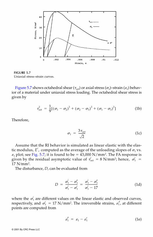
© 2001 By CRC Press LLC
Figure 5.7 shows octahedral shear (oct) or axial stress (�1)–strain (�1) behav-ior of a material under uniaxial stress loading. The octahedral shear stress isgiven by
(1b)
Therefore,
(1c)
Assume that the RI behavior is simulated as linear elastic with the elas-tic modulus, computed as the average of the unloading slopes of �1 vs.�1 plot; see Fig. 5.7; it is found to be � 43,000 N/mm2. The FA response isgiven by the residual asymptotic value of � 8 Nmm2; hence, �17 Nmm2.
The disturbance, D, can be evaluated from
(1d)
where the are different values on the linear elastic and observed curves,respectively, and � 17 N/mm2. The irreversible strains, , at differentpoints are computed from
(1e)
FIGURE 5.7Uniaxial stress–strain curves.
oct2 1
9--- �1 �2�( )2
�2 �3�( )2�1 �3�( )2
� �[ ]�
�13oct
2-----------�
Ei,
octc
�1c
D�1
i�1
a�
�1i
�1c
�-------------------
�1i
�1a
�
�1i 17�
-------------------� �
�1i
�1c
�1p
�1p
�1 �1e
��

© 2001 By CRC Press LLC
where
A plot of D vs. using Eqs. (1d) and (1e) is shown in Fig. 5.8. It can alsobe appropriate to use total strain, �1, with the plot of D vs. �1. Here weassumed that D is expressed only in terms of the axial strains; that is, theother two strains (�2 and �3) are not considered.
Now, the incremental Eq. (1a) can be integrated starting with the zero stressand strain at the origin, by writing it as
(1f)
where k denotes increment and � 0 because is a constant value. Also,we have assumed that the total stresses, and , are evaluated at the pre-vious increment.
Let the first strain increment � 0.0005. The RI stress increment isgiven by
The corresponding observed stress increment from Fig. 5.7 is found to beabout 21.0 N . Therefore,
As D0 � 0 at the origin, dD � 0.111 � 0.000 � 0.111.Therefore,
FIGURE 5.8Disturbance vs. irreversible strains: linear RI simulation.
�1e �1
43,000-----------------�
�1p
d�1 k( )a 1 Dk�( )Eid�1 k( )
i Dkd�1 k( )c dD �1 k�1( )
c�1 k�1( )
i�( )� ��
d�1c
�1c
�1c
�1i
d�1 1( )i
d�1 1( )i Ei 0.0005� 43,000 0.0005�� �
21.5� Nmm2
mm2
D121.5 21.0�21.5 17.0�----------------------------- 0.50
4.5---------- 0.111� � �
d�1 1( )a 1 0.111�( )21.5 0.111 17 0�( )��
0.889 21.5 5.661���
19.11� 1.887� 21.0 Nmm2�

© 2001 By CRC Press LLC
Now, consider the second strain increment, � 0.0005. The total strain� 0.0005 � 0.0005 � 0.001.
Therefore,
and
Hence,
Therefore, dD2 � 0.230 � 0.111 � 0.119, and
Therefore,
Consider the third increment as � 0.002. Therefore, the total strain �0.001 � 0.002 � 0.003.
Therefore,
d�1 2( )i
�1 2( )i
�1 2( )i 43,000 0.001��
43.00� Nmm2
�1 2( )a 37.00 Nmm2�
D243 37�43 17�-------------------- 6
26------ 0.23� � �
d�1 2( )a 1 0.230�( ) 43.0 21.5�( ) 0.119 17 21�( )��
16.55� 0.476� 16.09�
�1 2( )a 21.0 16.08� 37.08 Nmm2
� �
d�1 3( )i
�1 3( )i 43,000 0.003��
129.00� Nmm2
�1 3( )a � 39.00 Nmm2
D3129 39�129 17�----------------------- 90
112--------- 0.804� � �
dD3 0.804 0.23� 0.574� �
d�1 3( )a 1 0.804�( ) 129.00 37.00�( ) 0.574 17.00 43.00�( )��
0.196 92.00 14.92���
18.03 14.92� 3.11� �

© 2001 By CRC Press LLC
Therefore, � 37.08 � 3.11 � 40.19, which indicates the drop in theobserved stress after the peak stress.
The predicted stress–strain curve from the foregoing procedure is shown inFig. 5.9(a) and compares very well with the observed curve shown in Fig. 5.7.
Note 1. It is possible that in the early range of the stress–strain behavior,D will be negative. In that case, D can be assumed to be zero, as in that rangeno significant disturbance has occurred, and the RI and observed responsesare essentially the same.
Note 2. In the foregoing calculations, we have used the observed stressfrom the given stress–strain curve so as to calculate the disturbance, D. Thisis only for illustration purposes. In general, D can be calculated from thegraph of D vs. (plastic) strain (Fig. 5.8). Also, D can be expressed as
(1g)
FIGURE 5.9Comparison of observed and predicted behavior.
�1 3( )a
D Du 1 e A�p z( )
��( )�

© 2001 By CRC Press LLC
where Du corresponds to the ultimate or residual value. For instance, Du canbe calculated from the residual value of about 17.0 N/ (Fig. 5.7). Theirreversible strain trajectory (� ) is given by the total axial plastic strain, .The parameters A and Z are then found by using the procedure given inChapter. 3. Then, for a given total strain increment, the corresponding plasticstrain increment and total plastic strain, can be found. Substitution of Du,A, Z, and in Eq. (1g) gives the value of D. The increment or rate dD canalso be found by using Eq. (4.13), Chapter 4, as
(1h)
Figure 5.9(b) shows comparison of predicted and observed behavior obtainedby using dDk in Eq. (1h). The value of Du � 1.0 was assumed, and A � 651.80and Z � 1.03 were found by using the procedure in Chapter 3.
Note 3. The calculations can be improved by using small strain incre-ments and an iterative procedure. In the iterative procedure, the value ofthe total stress, at the end of the previous increment is used for the firstiteration during the increment. For subsequent iterations, the value of atthe previous iteration can be used. The iterations can be continued until con-vergence, that is, the two successive iterative values of show a small dif-ference � .
Example 5.2Consider that the RI response for the problem in Example 5.1 is characterizedas nonlinear elastic and that the stress–strain curve is simulated by using thehyperbola as
(2a)
where a and b are parameters related to the initial slope (Ei) and the asymp-totic stress, (Fig. 5.10).
In order to evaluate the RI stress, , we need to evaluate a and b, whichare given by
(2b)
(2c)
mm2
�1p
�1p,
�1p
dDk AZeA�k
p( )z�
�kp Z�1( )
�kp
�k�1p
�( )��
�1i ,
�1i
�1a ,
�
�1i �1
i
a b�1i
�------------------�
�1f
�1i
a1Ei---- 1
43,000---------------- 2.33 10 5�
�� � �
b1
� 1f
------ 175------ 0.0133� � �
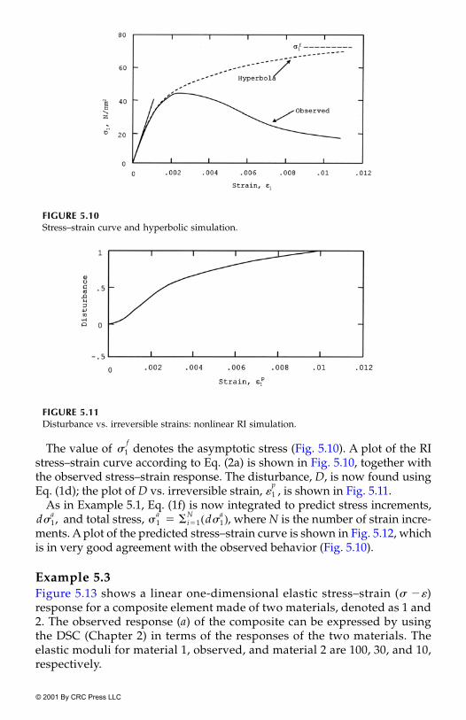
© 2001 By CRC Press LLC
The value of denotes the asymptotic stress (Fig. 5.10). A plot of the RIstress–strain curve according to Eq. (2a) is shown in Fig. 5.10, together withthe observed stress–strain response. The disturbance, D, is now found usingEq. (1d); the plot of D vs. irreversible strain, , is shown in Fig. 5.11.
As in Example 5.1, Eq. (1f) is now integrated to predict stress increments, and total stress, � , where N is the number of strain incre-
ments. A plot of the predicted stress–strain curve is shown in Fig. 5.12, whichis in very good agreement with the observed behavior (Fig. 5.10).
Example 5.3Figure 5.13 shows a linear one-dimensional elastic stress–strain (� ��)response for a composite element made of two materials, denoted as 1 and2. The observed response (a) of the composite can be expressed by usingthe DSC (Chapter 2) in terms of the responses of the two materials. Theelastic moduli for material 1, observed, and material 2 are 100, 30, and 10,respectively.
FIGURE 5.10Stress–strain curve and hyperbolic simulation.
FIGURE 5.11Disturbance vs. irreversible strains: nonlinear RI simulation.
�1f
�1p
d�1a , �1
a�i�1
N d�1a( )

© 2001 By CRC Press LLC
It is seen that the disturbance, D, is constant � 0.777; note that for compositematerials, disturbance has a different meaning compared to that for the samematerial element (Chapter 2). For example, at � � 0.10, � 10, � 3, and
� 1.0; therefore, D � (10 � 3)(10 � 1.0) � 0.777. Then the observedresponse, , can be found from
(3a)
For example, at � � 0.05:
Example 5.4The observed nonlinear elastic response (a), Fig. 5.14, is expressed by usinghyperbolic relation, Eq. (2a). The responses of the components of the compositematerial (1 and 2) are also expressed by using the hyperbolic relation. The
FIGURE 5.12Predicted stress–strain curves: nonlinear RI simulation.
FIGURE 5.13Composite material: two linear elastic components.
�1
�a
�2
�a
�a 1 D�( )�
1 D�2
��
�a 1 0.777�( )5 0.777 0.5���
1.50�

© 2001 By CRC Press LLC
parameters a and b, from Eq. (2a), are obtained from the initial slopes andasymptotic stresses as given in the following table.
Computation of stresses for different strains are shown below
Parameter Material 1 Observed (a) Material 2
E 43,000 N 31,500 20,000�f 75 N 55 35a 1/Ei � 2.33 � 10�5 3.18 � 10�5 5 � 10�5
b 1/�f � 0.0133 0.0182 0.0286
DSC Nonlinear Elastic as RI and FA Responses
� D
0 0 0 0 00.0005 16.69449 12.2399 7.77605 0.4994810.001 27.3224 20.02002 12.72265 0.5001720.002 40.08016 29.34703 18.65672 0.5009990.003 47.46835 34.74233 22.09131 0.5014780.004 52.28758 38.25921 24.3309 0.501790.005 55.67929 40.7332 25.90674 0.5020090.006 58.19593 42.56829 27.07581 0.5021720.008 61.6808 45.10854 28.6944 0.5023970.01 63.97953 46.78363 29.7619 0.502545
FIGURE 5.14Composite material: two nonlinear components.
mm2
mm2
�1 �a �2

© 2001 By CRC Press LLC
The value of D is essentially constant, at 0.50. For example, the observedstress for � � 0.005 is given by
Comment. As discussed in Chapter 2, the formulation of the DSC for anelement made of more than one material is referred to as multicomponentDSC, which is also described further in Chapter 8.
Example 5.5Figure 5.15 shows the observed bilinear response of a material; the yieldstress, �y � 1000 units. Assume that the RI response is simulated as linearelastic with Ei � 1000 units, and the FA response as �c � 0, i.e., Ec
� 0. Themodulus, after �y is 800 units. Evaluate the total and incremental stress fora typical strain, � � 2 units. The disturbance, D, is given by
(5a)
Consider two points, � � 1 and � � 2. Let us evaluate and at � � 2.The values of D at � � 1 and � � 2 are
FIGURE 5.15DSC bilinear elastic response.
�a 1 0.5�( )55.68 0.5 25.9���
27.84 12.95�( )�
40.79 Nmm2�
Ea,
D 1�
a
�i
-----��
�a d�
a
D1 1�
i
�i
----� 0; D2 118002000------------� 0.1 hence, ; dD 0.1.� � � � �
�2a 1 0.1�( )2000 0.1 0���
1800�

© 2001 By CRC Press LLC
Alternatively:
hence,
Example 5.6: Ceramic CompositeA ceramic composite was fabricated by using a special thermal liquefactionprocess (17–19) in which a mixture of finely ground basaltic rock and metal(stainless steel) fibers (about 15% by weight) was heated in a furnace undercycles of heating and cooling around the temperature of about 1100�C. Flatspecimens of 3.0 � 6.0 � 0.5 inch (7.6 � 15.2 � 1.3 cm) were tested under ten-sion and compression loading, unloading, and reloading cycles; two testswere performed for each of the plain and fiber-reinforced ceramic. In addi-tion to the stress–strain behavior, ultrasonic P-wave velocity and attenuationmeasurements were made at different locations on the specimen during theloading cycles (18, 19).
The DSC model was used by assuming the RI behavior to be linear elasticor elastoplastic (�0-model); the latter is considered in Chapter 7. The FAmaterial was defined using the assumption that it can carry only thehydrostatic stress. Table 5.1 shows material parameters for the DSC model.
TABLE 5.1
Typical Parameters for Typical Fiber-Reinforced Ceramic Composite Under Uniaxial Tension and Compression Tests (Disturbance parameters below are relevant to linear elastic RI simulation.)
Parameter Tension Compression
E 29 GPa 29 GPaν 0.24 0.24� 0.000741 0.1565� 0.75 0.76n 6.00 5.88a1 1.00 � 1.3 ��1 0.972 1.29R 167 MPa 25 MPah 0.003 0.044w 4.53 4.53s 2.03 2.03Du 1.0 1.00
d�a 1 0.1�( ) 2000 1000�( ) 0.1 0 0.1 0 1000�( )�����
900 100�( ) 800� �
�2a
�1a d�
a� 1000 800� 1800� � �
10 14� 10 14�

© 2001 By CRC Press LLC
The disturbance function was defined by using the following expression[Eq. (3.16a, Chapter 3]:
(6a)
where h, w, and s are material parameters and �D is the trajectory of deviatoricplastic strains.
Figures 5.16(a) and (b) show typical comparisons between predictions bythe DSC model and test data for the tensile and compressive behavior offiber-reinforced specimens 1 and 2, respectively. Here, parameters from testson specimen 2 were used to predict the tensile behavior of test specimen 1;and those from test 3 were used to predict the compressive behavior of test 2.Thus, these are considered to be independent validations. It can be seen thatthe prediction from the linear elastic simulation for the RI behavior providessatisfactory correlations with the test data.
5.7.1 Correlation with Crack Density
Hudson (20) proposed the following equation for crack density in a deform-ing (elastic) material. It was assumed that the mean shape of randomly dis-tributed cracks is circular and the wavelengths of elastic waves are largecompared with the size of cracks and with their separation distances, so thatthe mean over the statistical ensemble can be used to predict properties of asingle sample.
(6b)
(6c)
where U11 � 16(1 � ν0)/3(2 � ν0), U33 � 8(1 � ν0)/3, ν0 and V0 are the Poisson’sratio and P-wave velocity in the RI material, and V� is the observed root meansquare P-wave velocity. Here, Cd � where n is the open cracks per unitvolume, and a is the mean dimension (radius) of cracks (20).
D Du 1 1�D
h-----
w
�
s�
��
Cd
15 1 �0�( )2 1 2�0�( )----------------------------- 1 V
�2
V02
----------�
2U113 2�0� 7�0
2�
1 2�0�( )2----------------------------------------�
U33�
-------------------------------------------------------------------�
� 1 V�2
V02
---------�
�
na3,

© 2001 By CRC Press LLC
Figure 5.17 shows variations of Cd and disturbance, Dv, [computed by usingthe ultrasonic P-wave velocities, [Eq. (3.9), Chapter 3] with for the ten-sile test on the fiber-reinforced ceramic.] Both Cd and Dv increase during thevirgin (monotonic) loading. During unloading, they decrease because as the
FIGURE 5.16Comparisons between DSC predictions and test data for ceramic composites (18, 19):(a) tensile response of specimen 1; (b) compressive response of specimen 2. (With permissionfrom Elsevier Science.)
J2D

© 2001 By CRC Press LLC
tensile stress is removed, the cracks close. Then, during reloading and sub-sequent virgin loading, both increase. Thus, disturbance represents a meas-ure of crack density, and both show consistent trends for the tension testinvolving loading, unloading, and reloading.
Example 5.7: Cemented SandAs discussed in Chapter 2, the DSC can be used to characterize the behaviorof bonded materials such as rocks, concrete, and artificially cemented sand.Here, we consider cemented Leighton–Buzzard sand with bonding material(quick-setting cement) 5% by weight and 14% by weight of water (18, 19, 21).Cubic specimens (100 � 100 � 100 mm) sizes were tested using a multiaxial
FIGURE 5.17Crack density and disturbance during uniaxial loading, unloading, and reloading for ceramiccomposites (18).

© 2001 By CRC Press LLC
test device, under different stress paths (Fig. 3.16, Chapter 3) and mean pres-sures. Measurements were obtained both for the stress–strain and ultrasonic(pressure and attenuation) properties.
The RI behavior was simulated as linearly elastic. The elastic moduli andthe disturbance parameters are shown in Table 5.2. The FA response was sim-ulated by using the critical-state model from Chapter 4.
Figures 5.18 and 5.19 show comparisons between the predictions andobserved data for CTC (compression) and TE (extension) tests with �0 � 30and 45 kPa, respectively; descriptions of stress paths are given in Fig. 3.16 andChapter 7. Both the stress–strain and volume change behavior are predictedwell by the DSC model.
Figure 5.20 shows the variations of crack density and disturbance with for the CTC 30 test. During the virgin loading both increase. During
unloading, as the load is removed, the microcracks experience opening, andboth Cd and D show an increase. During reloading, both decrease due to thecoalescence of the microcracks. Then, after the end of reloading, during thevirgin loading, both increase again. These are considered to be consistenttrends for the compression test.
The foregoing Examples 5.6 and 5.7 show that even with the assumption oflinear elastic behavior for the RI response, the DSC model provides satisfac-tory predictions of the stress–strain and volumetric responses for the ceramiccomposite and cemented sand. However, if the response of a (granular) mate-rial involves such factors as coupling of volumetric response, it would bemore appropriate to adopt a plasticity model (e.g., �0-model) for the RIbehavior, because such a model allows for the volumetric coupling. Alterna-tively, it may be possible to consider such coupling by including the volumechange response in the disturbance function while using the linear elasticmodel for the RI response.
Example 5.8Consider a composite made of three materials, as in Fig. 5.21. The elastic mod-uli, E1 and E2, are equal to 43,000 and 31,500 N for materials 1 and 2,respectively. The observed behavior and that of material 3 are simulated as
TABLE 5.2
Parameters for Cemented Sand
Parameter Value
E 120 MPa0.353
m 0.23� 0.11
0.27h 0.007
w (average) 1.30s (average) 0.60
v
e0c
J2D
mm2

© 2001 By CRC Press LLC
nonlinear elastic using the hyperbolic relation in Eq. (2a); the parameters aand b are 5 � and 0.0286, and 1 � and 0.057, respectively. Two dis-turbances are defined with respect to the responses of materials 1 and 3 (D13)and materials 2 and 3 (D23) as
(8a)
(8b)
FIGURE 5.18Comparisons between DSC predictions and multiaxial compression (CTC: �0 � 30 kPa) testfor cemented sand. (From Refs. 18 and 19, with permission from Elsevier Science.)
10�5 10�4
D13�
1�
a�
�1
�3
�-------------------�
D23�
2�
a�
�2
�3
�-------------------�

© 2001 By CRC Press LLC
The values of the strains, stresses and disturbances are given below:
The observed response can be found as the average response from the twodisturbance conditions as
(8c)
� D13 D23
0 0 0 0 00.0005 21.5 15.75 7.77605 3.891051 0.779374 0.6723990.001 43 31.5 12.72265 6.369427 0.82656 0.7471920.002 86 63 18.65672 9.345794 0.878533 0.8264640.003 129 94.5 22.09131 11.07011 0.906544 0.8678990.004 172 126 24.3309 12.19512 0.924059 0.8933630.005 215 157.5 25.90674 12.98701 0.936045 0.9105980.006 258 189 27.07581 13.57466 0.944764 0.9230380.008 344 252 28.6944 14.38849 0.956598 0.9397930.01 430 315 29.7619 14.92537 0.964256 0.950557
FIGURE 5.19Comparisons between DSC predictions and multiaxial extension (TE: �0 � 45 kPa) test forcemented sand. (From Refs. 18 and 19, with permission from Elsevier Science.)
�1 �2 �a �3
�a 1 D13�( )�
1 D13�3 1 D23�( )�
2 D23�3
� � �[ ]2�

© 2001 By CRC Press LLC
FIGURE 5.20Crack density and disturbance during multiaxial loading, unloading, and reloading forcemented sand, CTC: �0 � 30 kPa (18).
FIGURE 5.21Composite material with three components: two linear elastic and one nonlinear elastic.

© 2001 By CRC Press LLC
For example, for � � 0.005, is computed as
References
1. Fung, Y.C., Foundations of Solid Mechanics, Prentice-Hall, Inc., Englewood Cliffs,New Jersey, 1965.
2. Malvern, L.E., Continuum Mechanics, MacMillan Publishing Co., New York,1966.
3. Timoshenko, S.P. and Goodier, J.N., Theory of Elasticity, 3rd Edition, McGraw-Hill Book Co., New York, 1970.
4. Desai, C.S. and Siriwardane, H.J., Constitutive Laws for Engineering Materials,Prentice-Hall, Englewood Cliffs, NJ, 1984.
5. Eringen, A.C., Nonlinear Theory of Continuous Media, McGraw-Hill Book Co.,New York, 1962.
6. Truesdell, C., Continuum Mechanics—The Mechanical Foundations of Elasticity andFluid Dynamics, Vol. 1, Gordon and Breach, Science Publishers, New York, 1967.
7. Franklin, J.N., Matrix Theory, Prentice-Hall, Englewood Cliffs, NJ, 1968.8. Kachanov, L.M., Introduction to Continuum Damage Mechanics, Martinus Nijhoft
Publishers, Dordrecht, The Netherlands, 1986.9. Seraphim, D., Lasky, R., and Li, C., Principles of Electronic Packaging, McGraw-
Hill, New York, 1989.10. Knecht, S. and Fox, L., “Integrated Matrix Creep: Application to Accelerated
Testing and Lifetime Prediction,” in Solder Joint Reliability, Lau, J.H. (Editor),Van Nostrand Reinhold, New York, 1995.
11. Sarihan, V., “Temperature Dependent Viscoplastic Simulation of ControlledCollapse Under Thermal Cycling,” J. of Electronic Packaging, ASME, 115, 1993,16–21.
12. Desai, C.S., Chia, J., Kundu, T., and Prince, J.L., “Thermomechanical Responseof Materials and Interfaces in Electronic Packaging: Part I – Unified ConstitutiveModel and Calibration; Part II – Unified Constitutive Models, Validation andDesign,” J. of Elect. Packaging, ASME, 119, 4, 1997, 294–300; 301–309.
13. Riemer, D.E., “Prediction of Temperature Cycling Life for SMT Solder Jointson TCE-Mismatched Substrates,” Proc. Electronic Component Conf., IEEE, 1990,418–423.
14. Skipor, A., Harren, S., and Botsis, J., “Constitutive Characterization of 63/37Sn/Pb Eutectic Solder Using the Bodner-Partom Unified Creep-Plasticity Model,”Adv. in Elect. Packaging, Proc. Joint ASME/JSME Conf. On Electronic Packaging,Chen, W.T. and Abe, H. (Editors), Vol. 2, 1992, 661–672.
15. Pan, T.Y., “Thermal Cycling-Induced Plastic Deformation in Solder Joints—Part I:Accumulated Deformation in Surface Mount Joints,” J. Electronic Packaging, ASME,113, 1991, 8–15.
�a
�a � 1 0.936�( )215 0.936 12.98 1 0.91�( )157.5 0.91 12.98�� 2� ����
51.902 25.95 Nmm2� �

© 2001 By CRC Press LLC
16. Chia, J. and Desai, C.S., “Constitutive Modelling of Thermomechanical Responseof Materials in Semiconductor Devices Using the Disturbed State Concept,”Report to NSF, Dept. of Civil Eng. and Eng. Mechs., University of Arizona, Tucson,AZ, USA, 1994.
17. Desai, C.S. and Girdner, K., “Structural Materials from Lunar SimulantsThrough Thermal Liquefaction,” Proc. Eng. Construction and Operations in SpaceII, ASCE, Denver, Colorado, 1992, 528–536.
18. Toth, J. and Desai, C.S., “Development of Lunar Ceramic Composites, Testing andConstitutive Modelling Including Cemented Sand,” Report, Dept. of Civil Engng.and Engng. Mechanics, University of Arizona, Tucson, Arizona, USA, 1994.
19. Desai, C.S. and Toth, J., “Disturbed State Constitutive Modeling Based onStress-Strain and Nondestructive Behavior,” Int. J. Solids & Struct., 33, 11, 1996,1619–1650.
20. Hudson, A., “Wave Speed and Attenuation of Elastic Waves in Material Con-taining Cracks,” Geophys. J., Royal Astron. Soc., 64, 1981, 113–150.
21. Desai, C.S., Jagannath, S.V., and Kundu, T., “Mechanical and UltrasonicResponse of Soil,” J. of Eng. Mech., ASCE, 121, 6, 1995, 744–752.

© 2001 By CRC Press LLC
6Theory of Plasticity in DSC
CONTENTS6.1 Introduction
6.1.1 Mechanisms6.1.2 Theoretical Development6.1.3 Yield Criteria6.1.4 Mohr–Coulomb Yield Criterion6.1.5 Continuous Yielding or Hardening Models6.1.6 Critical-State Concept6.1.7 Yield Surface6.1.8 Parameters in the CS Model6.1.9 Cap Model6.1.10 Advantages and Limitations of the CS and Cap Models
6.2 Incremental Equations6.2.1 Parameters and Determination from Laboratory Tests6.2.2 Cyclic Loading6.2.3 Thermoplasticity
6.3 Examples
6.1 Introduction
The development and application of the theory of plasticity have occurredover the last many years (1–13). The intention here is to describe briefly thebasic aspects of the theory and its use in the DSC.
The theory of elasticity (Chapter 5) is applicable if the material is elastic; thatis, upon removal of load, it returns to its original configuration along the samepath; see Fig. 6.1(a). However, except for limited ranges of loading, most mate-rials do not return to their original configuration; that is, they follow differentpaths during unloading. As a result, at the end of unloading, the materialretains a part of the deformation or strain, which is referred to as irreversible,inelastic, or plastic strain, . Hence, the total strain, �, at different points is�
p

© 2001 By CRC Press LLC
assumed to be composed of the plastic, , and the elastic or recoverable parts,; Fig. 6.1(b).If the material (element) is elastic up to point A and then yields plastically, as
in Fig. 6.1(b), it is referred to as elastoplastic material. If, after point A, it experi-ences continuing deformation under the constant yield stress (�y), it is calledelastic perfectly plastic material. After the yield point A, if the material isunloaded, it will not return to its original configuration and will experience plas-tic strain, .
The “stiffness” of some materials may experience gradual decrease duringyielding; however, the stress under continuing loading increases after theyield point. In other words, every point during the loading is a “new” yieldpoint, and the next yield stress is greater than the previous yield stress. Suchbehavior is called elastic-plastic hardening response.
Many materials, e.g., geologic, concrete, and polymers, may exhibit verylittle or no elastic region, and the point A0 is very near the origin [Fig. 6.1(b)].That is, they exhibit irreversible strains almost from the very beginning of
FIGURE 6.1Schematics of responses.
�p
�e
�p

© 2001 By CRC Press LLC
loading, and harden or yield continuously. Such a response is termed contin-uous hardening or yielding.
If, after reaching the peak stress, the stress experiences a decrease comparedto the peak stress, the response is called strain softening; see Fig. 6.1(c). Somematerials may first exhibit a drop in stress after peak, i.e., strain-softeningresponse, and then after a certain level of threshold strain (�t) may harden orstiffen. Such a behavior is called strain-softening-stiffening behavior [Fig. 6.1(d)].
6.1.1 Mechanisms
The manifestation of irreversible or plastic strains can be attributed to theinternal changes at the atomic and microlevels. At the atomic level, the bondscan stretch, causing a recoverable elastic response. Then relative slip canoccur, causing an irrecoverable response (5). In the elastic range, the materialparticles, see Fig. 6.2(a), maintain bonding or contact such that upon removal
FIGURE 6.2Mechanisms at the particle level.

© 2001 By CRC Press LLC
of the load, the material springs back to its original state. After yield, whichcan be considered as a threshold state, the contacts may experience relativemotions [Fig. 6.2(b)] such as translation along the contact. The measuredmacrolevel motions or displacements represent accumulation of motions thatoccur at the atomic and microlevels. A part of the accumulated motion (dis-placement) is not recovered when particles are unloaded. This is similar tothe behavior of two blocks [Fig. 6.2(b)] in which, upon unloading, a part ofthe displacement is not recovered. The motion (displacement) that is notrecovered is referred to as irreversible or plastic.
The cohesive part of the material strength is mainly present in the case of theelastic-perfectly-plastic materials. The continuing strains occur under con-stant yield stress, which represents the cohesive strength due to interparticleattraction and chemical bonds. Both the cohesive and frictional properties areoften present in many materials; hence, after the yield for an elastic-plastichardening material [Fig. 6.1(b)], the yield strength can increase with furtherloading.
In the case of strain-softening response [Fig. 6.1(c)], some of the interparticlebonds may experience breakage, resulting in the reduction in the stress thematerial can carry. However, for some materials and loading, after a certainreduction in stress and self-adjustment of the microstructure, the contacts mayreestablish and rebonding may occur with increasing strains; such a behaviorcan be called stiffening or healing; see Fig. 6.1(d). During softening, bondbreakage can occur, and during stiffening rebonding can occur; see Fig. 6.2(c).Such behavior is considered in Chapter 10.
6.1.2 Theoretical Development
From the above discussion, it is evident that in order to define the behaviorof an elastic-plastic material, it is required to define (a) the state at whichyielding occurs and (b) the behavior after yield so as to evaluate the plasticdeformations during the post-yield region.
6.1.3 Yield Criteria
A yield criterion defines the limit of the elastic regime and is usually expressedin terms of stresses. In the case of one-dimensional or uniaxial loading, the yieldcriterion can be expressed as
(6.1)
where F is the yield function and �y is the uniaxial tensile or compressivestress at which yielding occurs. In general, the yield criterion is expressed interms of the six components of stress as
(6.2)
u˜ r( )
u˜ r
p( )
F F �y( )�
F F �˜
( )�

© 2001 By CRC Press LLC
If we assume that the material is isotropic, i.e., its response is independentof the direction, F can be expressed as
(6.3)
where �1, �2, and �3 are the principal stresses. Often, the yield function isexpressed in terms of the invariants (J1, J2, J3) of the total stress tensor, �ij,
(6.4a)
Sometimes, it is appropriate to use the invariants, J2D, J3D, of the deviatoricstress tensor, Sij, as
(6.4b)
where
and
If the yield behavior of the material, like that of some metals and saturatedcohesive soils under undrained conditions, is affected only by the shearstress, then F is expressed as
(6.5a)
which leads to the well-known von Mises criterion (2, 6, 12)
(6.5b)
where k is the material parameter determined from laboratory tests. Hence,
(6.5c)
For uniaxial tension loading, if the yield stress is �y, then Eq. 6.5(c), gives
(6.5d)
F F �1, �2, �3( )�
F F J1, J2, J3( )�
F F J1, J2D, J3D( )�
J1 �ii; J212---�ij� ji
12---tr �
˜( )2; J3
13---�ik�km�mi
13---tr �
˜( )3;� � � � �
J2D12---SijSij J2
J12
6----�
16--- �1 �2�( )2
�2 �3�( )2�1 �3�( )2
� �[ ]� � �
J3D J323--- J1J2�
227------ J1
3�
13---SijSjmSmi
13---tr S
˜( )3
� � �
F F J2D( )�
F J2D k2� 0� �
16--- �1 �2�( )2
�2 �3�( )2�1 �3�( )2
� �[ ] k2�
13---�1
2 13---�y
2 k2� �

© 2001 By CRC Press LLC
Therefore,
(6.5e)
In the case of pure shear stress at yield, s, we can derive the following rela-tion:
(6.5f)
The von Mises criterion (F) plots as a cylinder, with constant radius,Fig. 6.3(a), in the principal stress space, indicating that the behavior is notaffected by the mean pressure, p � J1�3. The Drucker–Prager (D–P) yield cri-terion allows for the effect of mean pressure and is given by
(6.6a)
where � and k are material parameters. The D–P criterion plots as a right conein the stress space, indicating that the yield response is a function of the meanpressure, p. For conventional triaxial compression (CTC) loading (�1 � �2 ��3; Fig. 3.16), and for plane strain idealization, the values of � and k arerelated to the angle of friction, , and cohesion, c, as (12, 14–16)
CTC
(6.6b)
(6.6c)
Plane strain
(6.6d)
(6.6e)
6.1.4 Mohr–Coulomb Yield Criterion
The Mohr–Coulomb (M–C) yield criterion allows for the effect of friction andplots as an irregular hexagon in the stress space; see Fig. 6.3(b). One of theproperties of this criterion is that it includes different strengths under different
k�y
3-------�
s�y
3-------�
F J2D �J1 k�� 0� �
�2 sin
3 3 sin�( )------------------------------------�
k6c cos
3 3 sin�( )------------------------------------�
�tan
9 12 tan2�( )1�2
--------------------------------------------�
k3c
9 12 tan2�( )1�2
--------------------------------------------�
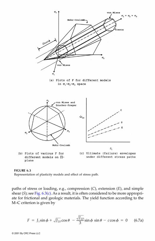
© 2001 By CRC Press LLC
paths of stress or loading, e.g., compression (C), extension (E), and simpleshear (S); see Fig. 6.3(c). As a result, it is often considered to be more appropri-ate for frictional and geologic materials. The yield function according to theM–C criterion is given by
(6.7a)
FIGURE 6.3Representation of plasticity models and effect of stress path.
F J1 J2D J2D
3-----------� sinsin c cos�cos�sin 0� �

© 2001 By CRC Press LLC
where is the Lode angle:
(6.7b)
and
(6.7c)
Hence, it includes the effect of the third invariant, J3D, of Sij, which is givenafter Eq. (6.4b).
6.1.5 Continuous Yielding or Hardening Models
In the classical plasticity models described above, the process of yieldingdepends on the state of stress; however, no consideration is given to thechanging physical state of the material due to internal microstructural trans-formations. During deformation, the material state changes continuously; forexample, the density, specific volume, or void ratio changes under bothhydrostatic and shear stresses. This can be particularly true in the case ofmaterials like geologic, concrete, and some ceramics, which exhibit a coupledresponse due to shear and hydrostatic loadings. As a consequence, the mate-rial may exhibit yielding (almost) from the very beginning, e.g., point A0 inFig. 6.1(b). That is, every point on the stress–strain response is a yield point,and the yield stress increases continuously. Continuous yielding may beattributed to internal microstructural changes due to relative particlemotions such as compaction, sliding, and rotation. The irreversible or plasticpart of these motions plays a significant role in continuous yielding, whichcan be expressed in terms of internal variables such as volumetric and devi-atoric plastic strain trajectories, and plastic work or dissipated energy.
In the context of geologic materials, mention may be made of Hvorslev’s(17) pioneering work on the behavior of remolded clays, Casagrande’s (18)idea of critical density or void ratio, the critical-state concept by Roscoe et al.(19, 20), and the cap models by DiMaggio and Sandler (21). Here, we shallbriefly describe the continuous yielding models based on the critical-stateand cap concepts.
6.1.6 Critical-State Concept
We first describe the basic idea in the critical-state (CS) concept. Irrespectiveof the initial density, a (granular) material, under shear stress, passes throughvarious deformation states and finally approaches the critical state at which itsvolume or density or void ratio does not change. In the critical state, the
13---sin 1� 3 3
2----------
J3D
J2D3�2
-------� �
�6----�
�6----� �

© 2001 By CRC Press LLC
material with a given initial mean pressure continues to deform under theconstant shear stress reached up to that state without further change in itsvolume (see Chapter 3).
Figure 6.4 shows symbolic stress–strain and volumetric responses undercompressive loading of initially loose and dense materials with given initialmean pressure, p0 � �0 � J10 �3. In the case of the loose material, the volumecontinuously decreases and then approaches the critical state (CS), denotedby c. The dense material may first compact (decrease in volume) and after aninstantaneous state of constant volume, which represents a threshold transi-tion, the material dilates, i.e., its volume increases. Finally, it approaches thesame critical state of invariant volume as that for the loose material under thegiven p0.
Laboratory testing of normally consolidated cohesive soils under undrainedand drained conditions leads to similar critical-state conditions. This isdepicted in Fig. 6.5(a) and (b) (12). Here it can be seen that shearing under dif-ferent initial mean pressures [p � (�1 � �3)�2] leads to invariant shear stresses( � �1 � �3) and void ratios ( ) at the critical state. The locus of such shear
FIGURE 6.4Behavior of loose and dense granular materials and critical state.
qc ec

© 2001 By CRC Press LLC
stresses at the critical state is often found to be a straight line on the q–p plot,shown in Fig. 6.5, which is called the critical-state line (CSL). The locus of thevoid ratios at the critical state on the e–�np plot, in Fig. 6.4(c), is often curvedbut is frequently approximated as the line with a slope of .
Now, if the two responses q–p and e–p are combined together, in Fig.6.6(a), they represent curved surfaces in the q–p–e plot. Thus, the behaviorof the material is now not only dependent on the state of stress (q, p), butalso on the physical state represented by void ratio (e) or density (�). Asshown in Fig. 6.6(b), the projection of the curved surface [Fig. 6.6(a)] on theq–p plot represents yield surfaces that grow continuously and intersect theCSL such that the tangent to the yield surface is horizontal; this implies thatthe change in the volumetric (plastic) strain at the intersection vanishes.Similarly, if the material is assumed to be isotropic, it will experience onlyvolumetric strains under hydrostatic loading and hence, the yield surfacewould intersect the p-axis at a right angle. In Fig. 6.6(b), and denote
FIGURE 6.5Undrained and drained behavior of granular materials.
�sp
�vp

© 2001 By CRC Press LLC
the plastic shear and volumetric strains, respectively, and d denotes incre-ment. In the earlier development of the critical-state concept (19, 20), theyield surfaces were considered elliptical.
The foregoing now permits definition of the material behavior under con-tinuous yielding and at the critical state. It may be noted that in the earlierwork (19, 20), the main emphasis was on the definition of the critical state,whereas the formulation, use, and implementation of the continuous yield-ing aspect became evident later, particularly in the context of computationalprocedures such as the finite-element method.
FIGURE 6.6Critical-state representation (12, 19, 20).

© 2001 By CRC Press LLC
There have been a number of subsequent works involving the formaliza-tion and use of the critical-state concept for describing behavior of materialssuch as overconsolidated clays (22) and rocks (23). However, because a mainobjective here is to discuss the hierarchical single-surface (HISS) approach,which includes the critical-state model as the special case, we present onlybrief descriptions of some aspects in the earlier critical-state models.
6.1.7 Yield Surface
The equation of the yield surface, Fy [Fig. 6.6(b)], according to the modifiedCam clay model, is derived as (19, 20)
(6.8)
where M is the slope of the CSL given by
(6.9)
and p0 is the varying value of mean pressure at the intersection of the yield sur-face with the p-axis, Fig. 6.6(b), during shearing, and denotes the yielding orhardening as function of the volumetric plastic strain or void ratio :
(6.10a)
Also, at the critical state:
(6.10b)
or
Here, and � are the slopes of the consolidation (isotropic) loading andunloading responses, respectively [Fig. 6.4(c)], is the value of corre-sponding to J1 � 3pa, pa is the atmospheric pressure constant, and is thevoid ratio at the critical state.
For the conventional triaxial stress condition (�1 � �2 � �3), q � �1 � �3 � and p � (�1 � 2�3)�3 � J1�3. Substitution in Eq. (6.8) gives the yield
surface in terms of the stress invariants (12) as
(6.11)
where J10 is the value of J1 at the intersection of the yield surface with the J1-axis.
M2p2 M2p0p� q2� 0�
q Mp�
d�vp( ) dev
p( )
d�vp dep
1 e0�--------------- ��( )
1 e0�-------------------
dp0
p0--------� �
ec e0c
� ln J1c�3pa( )�
J1c 3pae
e0c ec
�
-----------------
�
e0c ec
ec
3 J2D
M2J12 M2J1J10 27J2D�� 0�

© 2001 By CRC Press LLC
For the general three-dimensional case:
(6.12a)
(6.12b)
hence, the yield surface is expressed as
(6.13)
where is the slope of the critical-state line in – J1 space, and M �3 ; see Fig. 6.7.
6.1.8 Parameters in the CS Model
If the CS model is used in the context of elastoplastic behavior with isotropichardening (the yield surface grows symmetrically with respect to the origin inthe stress space), the following six parameters are required for the basic CSmodel:
Elastic: E and � or K and GPlastic: M, , � (for unloading), e0 (initial void ratio)
Details of their determination from laboratory tests are given subsequently.
6.1.9 Cap Model
The basic idea in the cap model is similar to that in the critical-state model. It wasproposed by DiMaggio and Sandler (21) to characterize the behavior of sands.In this model, Fig. 6.8, two functions are defined, one to characterize continuous
FIGURE 6.7Critical-state line on � J1 space.J2D
J2D16--- �1 �3�( )2
�2 �3�( )2�1 �3�( )2
� �[ ]�
p �1 �2 �3� �( )�3�
m2J1
2 m2J1J10� J2D� 0�
m J2D
3m

© 2001 By CRC Press LLC
yielding, Fy, and the other for the failure behavior, Ff, which is composed of aninitial portion of the Drucker–Prager surface and the ultimate part of the vonMises criterion, joined smoothly. This implies that in the early stage of loadingwhen the mean pressure is low, the material behaves as cohesive-frictional, andat higher mean pressure, it exhibits essentially cohesive response.
The expression for the yield caps, Fy , assumed to be elliptical, is given by
(6.14)
where J10 represents the intersection of the yield surface with the J1-axis [sim-ilar to p0 in the critical state (Cam clay) model], J1C is the value of J1 at the center
FIGURE 6.8Representation of cap model in �J1 stress space.J2D
FyJ10 J1c�
J2DC
--------------------
2
J2D J1 J1c�( )2� 0� �

© 2001 By CRC Press LLC
of the ellipse, and is the value of when J1 � J1c. The term J10 repre-sents hardening or yielding and is expressed in terms of volumetric plasticstrain as
(6.15)
where , W, and Z are material parameters; the latter denotes the size of thecap due to the initial (stress) conditions.
The expression for the failure surface is given by
(6.16)
where , , and are the material parameters.The yield caps intersect the failure surface, as shown in Fig. 6.8. As the load-
ing is applied, along a given stress path (P to Q), the material passes from oneyield surface to the next, and finally, at failure, the surface, Ff, is reached. As atfailure there is no volume change, Fy intersects Ff such that the tangent to Fy ishorizontal. Also, as the material is assumed to be isotropic, Fy intersects the J1-axis at a right angle. In computational analysis, it becomes necessary to designspecial schemes to handle the intersection point (B) while computing plasticstrain increments.
The number of parameters in the elastoplastic cap model is nine, whichincludes two elastic (e.g., E and � or K and G), , , and for the failure sur-face, and D, W, Z and R � (J10 � J1C)� for the yield cap (12, 21).
6.1.10 Advantages and Limitations of the CS and Cap Models
Both the critical-state (Cam-clay) and the cap models can provide improvedcharacterization of materials that exhibit continuous yielding. As a result, anumber of studies have used and implemented these models, often withmodifications, in computer procedures. However, they suffer from the follow-ing limitations in handling a number of important attributes of the behaviorof materials.
1. In both, the yielding is assumed to depend only on the volumetricplastic strains. It is found that for many materials, yielding can alsodepend on the deviatoric plastic strains. Hence, it is felt that bothshould be included in the definition of yielding.
2. The yield surface in both, Eq. (6.11) and Eq. (6.14), plot as circularin the principal stress space (�1��2, �3); this implies that thestrength of the material is independent of stress path. On theother hand, many (geologic and other) materials exhibit differentstrengths under different paths, e.g., compression, extension, andsimple shear; Fig. 6.3(c).
J2DC J2D
J101D----ln 1
�vp
W-----�
Z���
D
F f J2D �e� J1�
��� 0� �
� � �
� � �J2DC

© 2001 By CRC Press LLC
3. As can be seen from Figs. 6.6 and 6.8, the plastic strain increment,, is directed outward to the yield surfaces. If the compressive
volume change is considered to be positive in the positive J1-axis,this implies that up to the intersection of the yield surface with theCSL or the failure surface [Figs. 6.6(b) and 6.8(a)], the models wouldpredict compressive volume change. Then at the intersection, therewill be no volume change. In the case of the CS model, the yieldsurface is used in the calculations, then after the critical state isreached, the volume change will be zero. In the cap model, if Ff isused, volume change can occur after the failure and can involvedilation or volume increase as the plastic strain increment will nowbe directed in the negative J1-direction. In many materials, it isfound that the dilation may start before the peak or the failure isreached, point b in Fig. 6.4. Thus, these models cannot allow forthe occurrence of dilation before the peak or failure.
4. Although the issue of strain-softening response has been discussedin the context of the CS models and subsequent modifications, therehas been no consistent approach available for strain softening, thatallows for the discontinuous nature of the material due to micro-cracking.
5. Many (frictional) materials exhibit nonassociative response, that is,the plastic potential function, Q, is different from the yield function,F. The earlier CS and cap models have been based on associatedplasticity, i.e., .
Comments: To Hierarchical Single-Surface Models. The foregoing mod-els are presented for completeness. The hierarchical single-surface (HISS)plasticity models (Chapter 7) provide a unified approach, which includesmost of the foregoing and other plasticity models as special cases. It elimi-nates or reduces the above deficiencies and usually requires fewer parame-ters, compared to those in the previously available models of comparablecapacity. The HISS-�0 model (Chapter 7) is mainly used to characterize the RIresponse in the DSC model.
6.2 Incremental Equations
The consistency condition and the normality rule are given by (1–6)
(6.17a)
and
(6.17b)
d�˜
p
Q F�
dF 0�
d�˜
p
�Q��
˜
--------�

© 2001 By CRC Press LLC
where is the vector of plastic strain increments, Q is the plastic potentialfunction ( for associative plasticity), and is the scalar proportionalityparameter. Use of Eq. (6.17) leads to the incremental equations as (for detailsof derivations, see Chapter 7)
(6.18a)
(6.18b)
where is the elasticity matrix, and is the matrix representing the contri-bution of the plastic response.
6.2.1 Parameters and Determination from Laboratory Tests
Elasticity: For linear elastic and isotropic materials, , Eq. (6.18) isexpressed in terms of elastic moduli such as E, � or G and K. Procedures fortheir determination are given in Chapter 5.
Plasticity: For the von Mises criterion, Eq. (6.5), the yield stress, �y, in ten-sion or compression or cohesive strength, c, are needed. Figure 6.9(a) showsa uniaxial stress–strain curve from which the yield stress, �y , can be obtainedat the point where plastic action initiates. It represents the point after whichthe material will experience plastic strains upon unloading.
For nonfrictional materials, the cohesive strength, c, can be found from thevalue of shear stress (�) at peak or failure [Fig. 6.9(b)], which shows the enve-lope of shear stress, �, vs. normal stress, �. If the material possesses mainlycohesive strength, the Mohr envelope [Fig. 6.9(b)] will be horizontal with c asthe intercept along the shear stress (�) axis. For the Mohr–Coulomb criterion,Eq. (6.7a), the values of c and the angle of friction () are found from Mohrdiagrams; see Fig. 6.9(b).
For the Drucker–Prager criterion, Eq. (6.6), the values of � and k can befound from the values of cohesion, c, and friction angle, . Alternatively, �and k can be found from plots of � J1; see Fig. 6.9(c).
The parameters for the critical-state model (e.g., , , e0) can be found byusing the procedure described in Chapter 3.
The parameters for the cap model are , , and in Eq. (6.16) and , W,and Z and R(J10) in Eqs. (6.14) and (6.15). The laboratory stress–strain testresults are used to find peak (failure) stress, and plotted as in Fig. 6.10(a).The intercept of the von Mises envelope at larger values of J1, along ,gives the values of , and that for the D–P envelope (at J1 � 0) gives thevalue of � . For finding the value of` , we can select a point(s) on thetransition curve; see Fig. 6.10(a). Equation (6.16) can be now written as
(6.19a)
d�˜
p
Q F�
d�˜
C˜
epd�˜
�
C˜
ep Ce
˜C˜
p��
C˜
e C˜
p
C˜
e
J2D
m
� � � D
J2D
�� � �
e� J1� � J2D�
�-----------------------�

© 2001 By CRC Press LLC
Therefore,
(6.19b)
For no initial stress (or yielding) Z � 0. The value of and W can be foundfrom hydrostatic test data [Fig. 6.10(b)]. With Z � 0, Eq. (6.15) becomes
(6.20a)
FIGURE 6.9Parameters for different yield criteria.
�1J1----ln � J2D�
�-----------------------
��
D
J101D----� ln 1
�vp
W-----�
�

© 2001 By CRC Press LLC
where J10 � 3p, p � mean pressure. Therefore,
(6.20b)
and
(6.20c)
(6.20d)
FIGURE 6.10Parameters for cap model.
3pD ln 1�v
p
W-----�
��
�vp W 1 e 3pD�
�( )�
�v �ve
��

© 2001 By CRC Press LLC
Here, �v is the total volumetric strains, and is the elastic volumetric straingiven by
(6.20e)
where K is the bulk modulus. Hence,
(6.20f)
Now, we can select pairs of points on the loading part of the p vs. �v curves,shown in Fig. 6.10(b). Then, substitution of the values of p and �v in Eq. (6.20f)leads to two equations that are solved for W and . A number of pairs ofpoints can be used for finding average values of W and D.
The value of R � ( J10 � J1c)/ , Eq. (6.14), is required to define the sizeand shape of the yield caps, which can be represented as contours of constantvolumetric plastic strains. If the yield caps are elliptical, R is given by the ratioof the major to minor axes of the ellipse. For granular materials, the value ofR is often found in the range of 1.67 to 2.0.
6.2.2 Cyclic Loading
In this chapter, we have discussed the characterization only for monotonicloading, often referred to as virgin loading, in which the applied stress increasescontinuously. In Chapter 7, we shall discuss DSC models for cyclic loading.
6.2.3 Thermoplasticity
Behavior of materials can be influenced significantly by temperature and itsvariations, often together with mechanical loading. It is possible to incorpo-rate temperature effects by appropriate modification of the yield function, F.Details are given in Chapter 7, with respect to the HISS models; the modelspresented here can be considered special cases of the HISS models.
6.3 Examples
Example 6.1Consider a one-dimensional stress–strain response, Fig. 6.11, under uniaxialstress (�), and the following two yield functions:
(1a)
(1b)
�ve
�ve p
K----�
�v W 1 e 3pD��( )
pK----��
D
J2DC
F � �y� 0� �
F J2D k2� 0, k
�y
3-------� � �

© 2001 By CRC Press LLC
where �y is the yield stress. Derive specialized incremental plasticity equa-tions based on Eq. (6.18):
(1c)
Details are given in Chapter 7, Eq. (7.44).For the one-dimensional case, � �, � �, and ; here we have
ignored the effect of other strains. Therefore, from the yield function inEq. (1a), we have
(1d)
Hence,
FIGURE 6.11Uniaxial stress–strain curve.
d�˜
C˜
epd�˜
C˜
e C˜
p�( )d�
˜� �
C˜
e
C˜
e �F��
˜
------- �F��
˜
-------
T
C˜
e�
�F��
˜
-------
T
C˜
e �F��
˜
-------�
-----------------------------------------� d�˜
�
�˜
�˜
C˜
e E�
�F��------- �
��------- � �y�( ) 1� �
d� EE 1 1 E� � �
1 E 1� �----------------------------� d��
0.d��

© 2001 By CRC Press LLC
which indicates that there is no change in stress during yielding for the per-fectly plastic model.
For the yield function in Eq. (1b):
(1e)
Therefore,
Again indicating that for the von Mises criterion with the perfectly plasticmodel, there is no change in stress during yielding.
Example 6.2Assume that the RI behavior is simulated as linear elastic with modulus E,Fig. 6.11. Consider that the observed response during yielding is given by
(2a)
that is, the FA response is assumed to possess strength equal to the yieldstress, �y .
The disturbance, D, can be evaluated [Eq. (3.7a), (Chapter 3)] as
(2b)
In the linear elastic range, before �y,
(2c)
J2D16--- 2�
2( )�
2
3-----� �
F�
2
3----- k2
��
�F��-------
23---��
d� EE 2
3--- �
23--- � E�
23--- � E 2
3--- �
-------------------------------�
d��
E E�( )d� 0.d�� �
�a
�c
�y� �
D�
i�
a�
�i
�y�------------------�
D�
i�
i�
�i
�y�------------------ 0� �

© 2001 By CRC Press LLC
and after yield
(2d)
Hence, D vs. plastic strain, , is as shown in Fig. 6.12.The details of the evaluation of the observed stress-strain response are as
follows:Before �y:
because D � 0 and dD � 0.After �y:
FIGURE 6.12Disturbance vs. plastic strain: �
c�y .�
D �i
�i
�
�i
�y�------------------ 1� �
�p
�a 1 D�( )�
i D�c
��
1 0�( )�i 0 �
c�� �
i� �
d�a 1 D�( )d�
i Dd�c dD �
i�
c�( )� ��
1 0�( )d�i 0 0� � d�
i� �
�a 1 1�( )�
i 1 �c
�� �y� �
d�a 1 1�( )d�
i 1 d�y 0����
d�y 0� �

© 2001 By CRC Press LLC
because dD � 0 and d�y � 0 as �y is constant. This indicates that there is nochange in stress during yielding. Thus, the DSC model provides, as a special-ization, the classical perfectly plastic model.
Example 6.3Consider Example 6.2 and assume that the FA state does not carry any stress;therefore, � 0, and � �y during yielding. Then, the disturbance function,D, is given by
(3a)
Before �y:
After �y:
The plot of D vs. is given in Fig. 6.13.
FIGURE 6.13Disturbance vs. plastic strain: .
�c
�a
D�
i�
a�
�i
------------------�
D�
i�
a�
�i
------------------ 0� �
D�
i�
a�
�i
------------------ 1�y
�i
-----�� �
�p
�c 0.0�

© 2001 By CRC Press LLC
Now the observed stress–strain behavior can be predicted as follows:Before �y:
After �y:
Now,
Therefore,
Again indicating that there is no change in stress during yielding and withthe assumption that , the DSC leads to the classical perfectly plasticmodel.
�a 1 D�( )�
i� D�
c�
1 0�( )�i 0 �
c�� �
i� �
d�a 1 0�( )d�
i� 0 d�
c 0 �c
�i
�( )����
d�i
�
�a 1 1�
�y
�i
-----�
�i
1�y
�i
-----�
0���
�y
�i
----- �i
� �y� �
d�a 1 1�
�y
�i
-----�
d�i
1�y
�i
-----�
0��
dD 0 �i
�( )�
�y
�i
----- d�i dD �
i�( )���
D 1 �y �i( ) 1�
��
dD 0 �y 1�( ) �i( ) 2�
d�i
���
�y
�i( )2
----------- d�i
��
d�a �y
�i
----- d�i �y
�i( )2
----------- d�i
�i
�( )���
�y
�i
----- d�i �y
�i
----- d�i
���
0�
�c 0�

© 2001 By CRC Press LLC
Example 6.4Consider a composite made of two materials, a metal and concrete (ceramic).Figure 6.14 shows the (measured) behavior of the metal (material 1) as elasto-plastic, concrete (material 2) as strain softening, and the composite as plastichardening. The behavior of materials 1 and 2 is assumed to be simulated byusing the DSC model. In the case of the metal, the RI behavior is simulated as lin-ear elastic, and the FA stress, � 59.00 ksi, is assumed; see Fig. 6.15(a). For con-crete, the RI response is considered as nonlinear (hardening) with � 6.0 ksi,Fig. 6.15(b).
The behavior of the metal and that of concrete were first computed byusing the following equations at step k (with d � 0):
(4a)
(4b)
(4c)
(4d)
Now, the observed stresses at various points (k) for the metal and concretewere used to evaluate the disturbance for the composite as
(4e)
where is the observed composite stress at point k at a given strain level.Then the predicted composite behavior was obtained by integrating the
FIGURE 6.14Behavior of metal, concrete, and composite: 1 psi � 6.89 kPa.
�c
�c
�c
d�ka 1 Dk�( ) �k
i�k�1
i�( ) dDk �k
c�k�1
c�( )��
Dk�k
i�k
a�
�ki
�c
�-------------------�
dDk Dk Dk�1��
�ka
�k�1a d�k
a��
Dk�k
1a�k
a�
�k1a
�k2a
�-----------------------�
�ka

© 2001 By CRC Press LLC
following equation:
(4f)
where dDk � Dk � Dk�1. Figure 6.16 shows that the predicted behavior of thecomposite compares very well with the observed behavior.
Some of the following practice examples may require calculations usingiterative procedures. It may be useful to prepare computer routines for suchiterative procedures. As necessary, appropriate values of parameters such asE can be adopted.
Example 6.5Assume that the RI behavior is simulated as bilinear elastic (see Fig. 5.15,Chapter 5). By assuming that (a) � � �y and (b) � 0, � �y , predictthe observed (elastic perfectly plastic) response.
FIGURE 6.15DSC responses for metal and concrete: 1 psi � 6.89 kPa.
d�ka 1 Dk�( )� d�k
1a Dkd�k2a dDk �k�1
2a�k�1
1a�( )��
�a
�c
�c
�a

© 2001 By CRC Press LLC
Example 6.6Assume that the RI behavior is simulated by using the hyperbolic relation,Eq. (2a), Example 5.2. Then predict the elastic perfectly plastic stress–strainbehavior assuming that (a) � � �y , and (b) � 0, � �y.
Example 6.7Predict the elastic plastic behavior assuming the RI behavior to be elastic (E),and the Drucker–Prager yield criterion, Eq. (6.6a).
References
1. Prager, W., “Recent Developments in Mathematical Theory of Plasticity,” J. ofAppl. Phys., 2013, 1949, 235–241.
2. Hill, R., The Mathematical Theory of Plasticity, Oxford Univ. Press, Oxford, 1950. 3. Drucker, D.C., “A More Fundamental Approach to Plastic Stress-Strain Rela-
tions,” Proc. First U.S. Nat. Congr. Appl. Mech., 1951, 487–491. 4. Drucker, D.C., “A Definition of Stable Inelastic Material,” ASME Trans., 81,
1959, 101–106. 5. Callister, W.D., Material Science and Engineering—An Introduction, John Wiley &
Sons, New York, 1985. 6. Bridgeman, P.W., Studies in Large Plastic Flow and Fracture with Special Emphasis
on the Effects of Hydrostatic Pressure, McGraw-Hill Book Co., New York, 1952. 7. Fung, Y.C., Foundations of Solid Mechanics, Prentice-Hall, Inc., Englewood Cliffs,
NJ, 1965. 8. Malvern, L.E., Introduction to Mechanics of Continuous Medium, Prentice-Hall,
Inc., Englewood Cliffs, NJ, 1969. 9. Kachanov, L.M., Foundations of Theory of Plasticity, North-Holland Publishing
Co., Amsterdam, 1971.10. Mendelson, A., Plasticity: Theory and Applications, MacMillan Publ. Co., New
York, 1968.
FIGURE 6.16Comparison of predicted and observed behavior of composite: 1 psi � 6.89 kPa.
�a
�c
�c
�a

© 2001 By CRC Press LLC
11. Owen, D.R.J. and Hinton, E., Finite Elements in Plasticity: Theory and Practice,Pineridge Press, Swansea, U.K., 1980.
12. Desai, C.S. and Siriwardane, H.J., Constitutive Laws for Engineering Materials,Prentice-Hall, Inc., Englewood Cliffs, NJ, 1984.
13. Chen, W.F. and Han, D.J., Plasticity for Structural Engineers, Springer-Verlag,New York, 1988.
14. Reyes, S.F. and Deere, D.U., “Elastic-plastic Analysis of Underground Openingsby the Finite Element Method,” Proc. 1st Int. Cong. Rock Mech., Vol. II, Lisbon,1966, 477–486.
15. Christian, J.T. and Desai, C.S., “Constitutive Laws for Geologic Media,” Chap-ter 12 in Numerical Methods in Geotechnical Engineering, C.S. Desai and J.T.Christian (Editors), McGraw-Hill Book Co., New York, 1977.
16. Desai, C.S. and Abel, J.F., Introduction to the Finite Element Method, Van NostrandReinhold Co., New York, 1972.
17. Hvorslev, M.J., “Physical Properties of Remolded Cohesive Soils,” Translation69-5, U.S. Army Corps of Engineers Waterways Experiment Stn., Vicksburg,MS, June 1969.
18. Casagrande, A., “Characteristics of Cohesionless Soils Affecting the Stabilityof Slopes and Earth Fills,” J. Boston Soc. Civil Eng., 1936, 257–276.
19. Roscoe, A.N., Schofield, A., and Wroth, P.C., “On Yielding of Soils,” Geotech-nique, 8, 1958, 22–53.
20. Schofield, A.N. and Wroth, P.C., Critical State Soil Mechanics, McGraw-Hill BookCo., London, 1968.
21. DiMaggo, F.L. and Sandler, I., “Material Model for Granular Soils,” J. Eng.Mech., ASCE, 97, 3, 1971, 935–950.
22. Banerjee, P.K. and Yousif, N.B., “A Plasticity Model for Mechanical Behaviourof Anisotropically Consolidated Clay,” Int. J. Numer. Analyt. Meth. Geomech., 10,5, 1986, 521–541.
23. Brown, E.T. and Yu, H.S., “A Model for the Ductile Yield of Porous Rock,” Int.J. Numer. Analyt. Meth. Geomech., 12, 6, 1988, 679–688.

© 2001 By CRC Press LLC
7Hierarchical Single-Surface PlasticityModels in DSC
CONTENTS7.1 Introduction
7.1.1 Basic HISS Model7.2 Specializations of the HISS Model
7.2.1 Classical Plasticity Models7.3 HISS Versions7.4 Material Parameters
7.4.1 Curved Ultimate Envelope7.4.2 Relation Between Ultimate Parameters, Cohesion,
and Angle of Friction 7.4.3 Bonding Stress, R7.4.4 Phase or State Change Parameter7.4.5 Hardening or Growth Parameters7.4.6 Nonassociative �1-Model7.4.7 Thermal Effects on Parameters7.4.8 Rate Effects
7.5 Repetitive Loading7.5.1 Dynamic Loading
7.6 The Derivation of Elastoplastic Equations7.6.1 Details of Derivatives
7.7 Incremental Iterative Analysis7.7.1 Possible Stress States7.7.2 Elastic-Plastic Loading7.7.3 Correction Procedures7.7.4 Subincrementation Procedure
7.8 Drift Correction Procedure7.9 Thermoplasticity7.10 Examples7.11 Stress Path
7.11.1 Stress Path Analysis of the HISS Model7.12 Examples of Validation
7.12.1 Examples of Geologic Materials7.12.2 Repeated Loading and Permanent Deformations

© 2001 By CRC Press LLC
7.1 Introduction
The hierarchical single-surface (HISS) plasticity models provide a general for-mulation for the elastoplastic characterization of the material behavior. Thesemodels, which can allow for isotropic and anisotropic hardening, and associ-ated and nonassociated plasticity characterizations, can be used to representmaterial response based on the continuum plasticity theory (1–6). In the caseof the DSC, they can be used to represent the RI response; in many cases, thebasic and simplest version, HISS-�0, that allows for isotropic hardening andassociated response has been used. It may be mentioned that use of plasticitytheory is one of the possible ways to characterize the RI behavior. However,the DSC can be formulated by simulating the (RI) response as nonlinear withirreversible deformations, without invoking the theory of plasticity.
We will present comprehensive details of the HISS approach including itstheoretical background, specializations, nature of parameters and their deter-mination from laboratory tests, details of parameters for typical materials,derivation of elastoplastic equations, incremental iterative analysis, and val-idations of the models for a number of materials: geologic, concrete, metals,alloys, silicon, etc.
It is useful to emphasize one of the important advantages offered by thehierarchical nature of the HISS model. Most other available models providefor a specific characteristic of the material behavior. On the other hand, theHISS (and DSC) approach provides for hierarchical adoption of models ofincreasing sophistication, say, linear elastic to nonassociated elastoplastic toelastoplastic with softening (disturbance). Thus, the user can select the mostappropriate model for a given material in specific engineering application. Inthis context, it is shown that the classical such as von Mises, Mohr–Coulomb,and Drucker–Prager, continuous yielding such as critical-state and capped(see Chapter 6), and other models such as by Matsuoka and Nakai (7), Ladeand co-workers (8, 9), and Vermeer (10) can be derived as special cases of theHISS model. It is also indicated that the anisotropic and kinematic versionsof the HISS model can provide alternative characterizations to models pro-posed by Mroz and co-workers (11–13), Krieg (14), Prevost (15), and Dafaliasand co-workers (16, 17).
7.1.1 Basic HISS Model
Consider the associated plasticity model in the hierarchical single-surface(HISS) approach. The yield function, F, is given by
(7.1)
F J2D �J1n
� �J12
�( ) 1 �Sr�( )m� 0� �
J2D FbFs� 0� �

© 2001 By CRC Press LLC
Here, � J2D� , where pa is the atmospheric pressure constant; � (J1 �3R)�pa, where R � the bonding stress (e.g., tensile strength under compressiveloading and compressive strength under tensile loading); n � phase changeparameter where the volume change transits from compaction to dilation orvanishes; m � �0.5 is often used; � � parameter related to the (ultimate) yieldsurface, � is related to the shape of F in the 1–2–3 space, Sr � stress ratio �
and � is the growth or hardening parameter, which can beexpressed in terms of internal variables such as plastic strain trajectory or accu-mulated plastic strains, and plastic work or dissipated energy. Based on thedevelopment of the hardening function for a wide range of “solid” materials,interfaces and joints, it was found that use of the plastic strain trajectory pro-vides a more consistent formulation than that by plastic work. Moreover, it isrelatively easier to compute the plastic strain trajectory from available test data.Hence, the plastic strain trajectory is commonly used in this text.
A simple form of � is given by
(7.2)
where is the trajectory of plastic strains, d denotesincrement, � is composed of deviatoric (�D) and volumetric (�v) plastic straintrajectories:
(7.3)
Here, is the deviatoric plastic strains tensor = , and� volumetric plastic strain. Figure 7.1(a), (b), and (c) show schemat-
ics of F � 0 in , octahedral plane, and 1–2–3 stress spaces. Theexpanding yield surfaces are continuous and approach the final or ultimateyield surface when � � 0. The points on the yield surfaces with horizontaltangents denote zero volume change or critical-state line (Chapter 6).
In the case of nonassociated plasticity, the plastic potential function, Q, isexpressed as (1, 3, 5, 18–20)
(7.4)
where h � correction function, which is introduced, for simplicity, throughthe hardening function as
(7.5)
where �0 � value of � at the end of initial (hydrostatic) loading, and � is thenonassociative parameter, and rv � �v/�.
J2D pa2 J1
27�2( ) J3D �J2D3� 2( ),
�a1
�n1
------�
� � d ijp d ij
p( )1� 2� ij
p,
� �D �v� dEijp dEij
p( )1� 2 1
3------- ii
p��� �
Eijp
ijp 1�3( ) ii�ij�
iip
vp
�J2D J1�
Q F h Ji, �( )��
�Q � � �0 ��( ) 1 rv�( )��

© 2001 By CRC Press LLC
FIGURE 7.1 Plots of F in different stress spaces (1–3).

© 2001 By CRC Press LLC
7.2 Specializations of the HISS Model
Before presenting derivations of the incremental constitutive equations, wediscuss various specializations of the HISS model.
7.2.1 Classical Plasticity Models
The parameter � in Eq. (7.1) defines the shape of the yield surface, F, in theprincipal stress space, Fig. 7.1(b). In the context of the theory of plasticity inwhich it is required that F be convex, the value of � is limited by � � 0.76 (seeExample 7.1). If it is assumed that (� � 0) and n � 2, Eq. (7.1) becomes (here,the overbar is deleted for convenience)
(7.6)
where 3R is the intercept along the J1-axis denoting tensile or compressivebonding stress; see Fig. 7.1(a).
Equation (7.6) can represent various classical plasticity models such as vonMises, Tresca, Drucker–Prager, and Mohr–Coulomb if there is no continuousyielding involved before the failure (ultimate) yield envelope is reached.Hence, as � � 0 at the ultimate condition, we have
(7.7a)
Now, 3R in Fig. 7.1(a) can be expressed approximately as
(7.7b)
where is the intercept along the -axis at J1 � 0 and is related to the cohe-sive (or tensile) strength of the material. Substitution of 3R in Eq. (7.7a) leads to
(7.7c)
If the effect of is ignored, Eq. (7.7c) reduces to
(7.7d)
which has the same form as the Drucker–Prager yield criterion, Eq. (6.6a) ofChapter 6. Now, if the effect of J1 is ignored, Eq. (7.7d) becomes
(7.7e)
which has the same form as the von Mises criterion, Eq. (6.5b) of Chapter 6.
F J2D � J1 3R�( )2� J1 3R�( )2
�� 0� �
F J2D �J12
� 6�J1R� 9�R2� 0� �
3Rc�
-------�
c J2D
J2D �J12
� 2 �c J1� c2
� 0�
J12
J2D 2 � c( )J1� c2
� 0�
J2D c2
� 0�

© 2001 By CRC Press LLC
If we assume that the material (soil) is normally consolidated or cohesion-less and 3R � 0, Eq. (7.6) becomes
(7.8)
which has the form similar to the modified Cam Clay model in the criticalstate soil mechanics, Eq. (6.11) of Chapter 6. In the Cam Clay model, p0
denotes the hardening parameter, which is dependent on the volumetricplastic strain or void ratio. In the HISS model, the hardening function, �, candepend on the total plastic strain trajectory �, Eq. (7.2), which includes boththe volumetric and deviatoric plastic strains, thereby providing a generaliza-tion of the continuous yielding or hardening process.
In the cap model, failure and continuous yield surfaces are defined (seeChapter 6). In the HISS model, at the ultimate, � � 0, and we have Eq. (7.7d),which is analogous to the failure surface, Ff [Eq. (6.16), Chapter 6] in the capmodel. Also, Eq. (7.6) is analogous to the continuous yield surface, Fy , inEq. (6.14) of Chapter 6.
Matsuoka and Nakai (7) proposed the following (yield) criterion (for cohe-sionless materials) as expanding open surfaces (Fig. 7.2):
(7.9a)
and Lade and co-workers (8, 9), proposed the following similar criterion (Fig.7.2):
(7.9b)
Both above criteria can be expressed as special cases of the F [Eq. (7.1)] in theHISS model. Subsequently, Lade and co-workers (9) modified their criterionto include closed and continuous yield surfaces, similar to the closed contin-uous yield surfaces in the HISS model (21, 22).
The model proposed by Vermeer (10) introduces the effect of both shearand plastic strains on the hardening response. The total strain increment (orrate), d , is expressed as
(7.9c)
where and are the incremental plastic strains due to shear and iso-tropic compression, respectively. It uses the criterion by Matusuoka and Nakai(7), Eq. (7.9a), to define the yield function relevant to plastic shear strains as
(7.9d)
where the hardening function, , is dependent on the plastic shear strain mobilized angle of friction (�m), peak friction angle (at failure) �p, and shear
J2D �J12
�J12
�� 0�
F J1J2 �1J3� 0� �
F J13
�2J3� 0� �
d ˜
d ˜
e d ˜
ps d ˜
pc� ��
d ˜
ps d ˜
pc
Fps J1J2 �J3� 0� �
� �p,

© 2001 By CRC Press LLC
modulus G0 at isotropic stress (J10 �3). A plastic potential function is definedto introduce the effect of volume dilitancy. A specific yield function is definedfor volumetric response as
(7.9e)
where and are material constants, is another hardening function forvolumetric response. The model can involve two (or more) constants todefine elastic response, and five for the plastic response for cohesionlessmaterials. For cohesive materials, the number of constants will be higher.Although this model involves effects of both the volumetric and deviatoricplastic strains on the hardening or yielding behavior, it is felt that their sepa-ration may not be necessary. The HISS models unify them and also allow theflexibility of using one or both terms in Eq. (7.3).
FIGURE 7.2Plots of open yield and failure surfaces in Lade et al. (8). ©1975, with permission from ElsevierScience.
Fpc
0c J1
J10------
�
pc
��
0c
� pc

© 2001 By CRC Press LLC
Table 7.1(a)to (c)shows outlines of various models and their chronologicaldevelopment and comparison of HISS models with other models. It can beseen from the descriptions herein that the HISS models provide improvedcharacterization with an equal or fewer number of parameters for compara-ble capabilities of other available models.
7.3 HISS Versions
The basic �0 version of the HISS approach is based on associative plasticity.Various hierarchical models for the inclusion of additional factors have beendeveloped: nonassociative �1-model (19, 20), kinematic and anisotropic hard-ening �2-models for sands and clays (26–28), and viscoplastic �vp (29–31). It isfound that the basic �0-model is usually sufficient to characterize the RIresponse of many materials. With the disturbance, D, in the DSC, and the RIresponse modelled using the �0-model, the nonassociative and anisotropicbehavior are accounted for, to some extent. This is because the disturbance,D, causes the deviation from normality of the plastic strains with respect to F(32). Hence, the major attention here is given to the �0-model.
7.4 Material Parameters
The elasticity parameters E, , G, and K are determined from laboratorystress–strain and volumetric behavior, as described in Chapter 5. Their valueswill depend on the measured response under a given stress path; see Fig. 7.3(c).For example, E and � can be found from different stress paths as follows:
Test E v
CTCRTE
CTERTC
TCTE —
SS —
1 Si � (average) slope of the unloading/reloading curve, �oct vs.(i � 1, 2, 3) plot.
2 CTC (1 � 2 � 3), and so on.
�
32
-------S12 S1
S2 S3�------------------------
3 2 S1 S2 S3�( )4 S1 S2 S3� �( )
-------------------------------------------------S2 S3�
4 S1------------------------
23
------- 1 v�( ) S1 S2 S3� �( )
32 2---------- 1 v�( ) S1 S3�( )
i

© 2001 By CRC Press LLC
TABLE 7.1(a)
Review of Various Models (From Ref. 21, with permission from Elsevier Science)
ModelYield function, F
Potential function, QNumber of Constants
and Comments
1. Classical plasticity (see Chapter 6)
F � (J1, J2D, c, �) � 0Q � F
Constants: 3 or 4One failure surface definesplastic behavior.
2. Critical state (23; see also Chapter 6)
Fy � Fy[J1(or p),J2D(or q), �,�, M, e0] � 0
Fc � Ff [J1(or p),J2D(or q), M] � 0
Q � F
Constants: 6Fy (below Fc) definescontinuous yielding, and Fc
defines critical or failure state.
Later modifications consider nonassociative behavior.
3. Cap models (see Chapter 6)
Fy � Fy[J1, J2D, R, D, W, Z] � 0
Fc � Ff[J1, J2D, ,, ) � 0
Q � F
Constant: 9Fy (below Ff) defines
continuous yielding, and Ff
defines failure surface.
4. Matsuoka and Nakai (7) F is open failure surface.
5. Lade (8) Constants: 13F gives open (failure) surface.
6. Desai (HISS) (1–6) Constants: 7 to 8 for �0
8 to 9 for �1
Single surface F for continuous yielding and ultimate, including failure, peak, and critical state.
7. Schreyer (24) Constants: 10Single surface F definescontinuous yielding approaching the failure or stationary state.
8. Kim and Lade (9) Constants: 11Single surface F definescontinuous yielding. Failure is defined by a separate function.
�
� �
FJ1 J2
J3--------- constant� 0� �
F J13
J3---- constant� 0� �
Fc spherical cap�
Q J13
� J3��
FJ2D
pa-------
2
FbFs� 0� �
F �J1
3---- L� 3� 0� �
F f 1 f 2 0� �
f 1 �1J1
3
J3----
J12
J2----�
�
f 2J1
pa----
h
eq�
Q q1 q2�
q1 �1J1
3
J3----
J12
J2----� �2�
�
q2J1
pa----
�
�

© 2001 By CRC Press LLC
The parameters in the HISS �0-model are � and � associated with the ulti-mate yield envelope [Figs. 7-1(a) and (b)], n associated with the transition (orphase change) from contractive to dilative or zero volume change, and � thehardening or growth function, which is expressed as a function of the plasticstrain trajectory, �, Eq. (7.3), which is composed of the deviatoric plastic straintrajectory, �D, and volumetric plastic strain trajectory �V, given by
(7.10a)
TABLE 7.1(b)
Comparison of �0 and Cap (Critical-State) and Lade Models
Model �0 Cap Model
Number of functions for the yield surface
1 2
Number of constants 5 � 2 (linear elastic constants) 7 � 2 (linear elastic)�2 (nonlinear elastic)
CapabilitiesHardening Total plastic strains Volumetric plastic strainsShear dilation Before peak stress At the peak stress onlyDifferent strength in different stress paths
Yes No
Modifications for added features
Systematic hierarchical additions
No systematic hierarchical method available
Comparison with Lade’s ModelLade and co-workers’ model with nonassociative plasticity model involved about 13constants. Recently they modified their model by incorporating single continuous sur-faces as in the HISS models; with the modification, the number of constants is 11 (9).
TABLE 7.1(c)
Comparison of Models for Cyclic Behavior of Clays
ModelHISS-�2
(26)Bounding Surface
Model (16, 17)Mroz, Prevost’s Model
(12, 13, 15, 25)
Number of functions for the yield surface
1 3 Multiple moving surfaces with similar shape
Number of constants 9 19 5 � 10 � m where m is the number of yield surfaces.For the example presented, the number of constants is 95.
Induced anisotropy Yes No YesPrediction of behavior of NC soil
Yes Yes Yes
Predicting shear-induced volumetric changes in drained tests or shear-induced pore pressures in undrained test for OC clay
Yes Yes Yes
�D dEijp dEij
p( )1� 2��
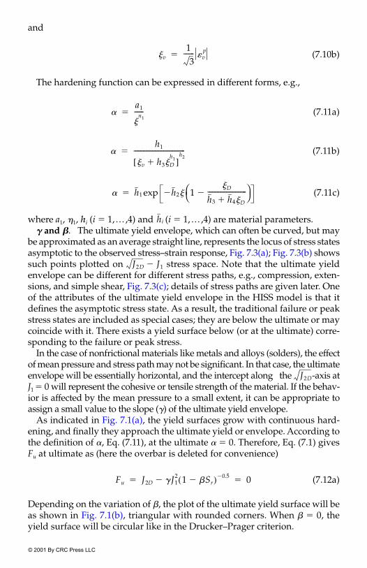
© 2001 By CRC Press LLC
and
(7.10b)
The hardening function can be expressed in different forms, e.g.,
(7.11a)
(7.11b)
(7.11c)
where a1, �1, hi (i � 1,…,4) and (i � 1,…,4) are material parameters.� and �. The ultimate yield envelope, which can often be curved, but may
be approximated as an average straight line, represents the locus of stress statesasymptotic to the observed stress–strain response, Fig. 7.3(a); Fig. 7.3(b) showssuch points plotted on stress space. Note that the ultimate yieldenvelope can be different for different stress paths, e.g., compression, exten-sions, and simple shear, Fig. 7.3(c); details of stress paths are given later. Oneof the attributes of the ultimate yield envelope in the HISS model is that itdefines the asymptotic stress state. As a result, the traditional failure or peakstress states are included as special cases; they are below the ultimate or maycoincide with it. There exists a yield surface below (or at the ultimate) corre-sponding to the failure or peak stress.
In the case of nonfrictional materials like metals and alloys (solders), the effectof mean pressure and stress path may not be significant. In that case, the ultimateenvelope will be essentially horizontal, and the intercept along the -axis atJ1 � 0 will represent the cohesive or tensile strength of the material. If the behav-ior is affected by the mean pressure to a small extent, it can be appropriate toassign a small value to the slope (�) of the ultimate yield envelope.
As indicated in Fig. 7.1(a), the yield surfaces grow with continuous hard-ening, and finally they approach the ultimate yield or envelope. According tothe definition of �, Eq. (7.11), at the ultimate � � 0. Therefore, Eq. (7.1) givesFu at ultimate as (here the overbar is deleted for convenience)
(7.12a)
Depending on the variation of �, the plot of the ultimate yield surface will beas shown in Fig. 7.1(b), triangular with rounded corners. When � � 0, theyield surface will be circular like in the Drucker–Prager criterion.
�v13
------- vp
�
�a1
�n1
------�
�h1
�v h3�Dh1�[ ]
h2---------------------------------�
� h1 h2� 1�D
h3 h4�D�-------------------------�
�exp�
hi
J2D J1�
J2D
Fu J2D �J12 1 �Sr�( ) 0.5�
� 0� �
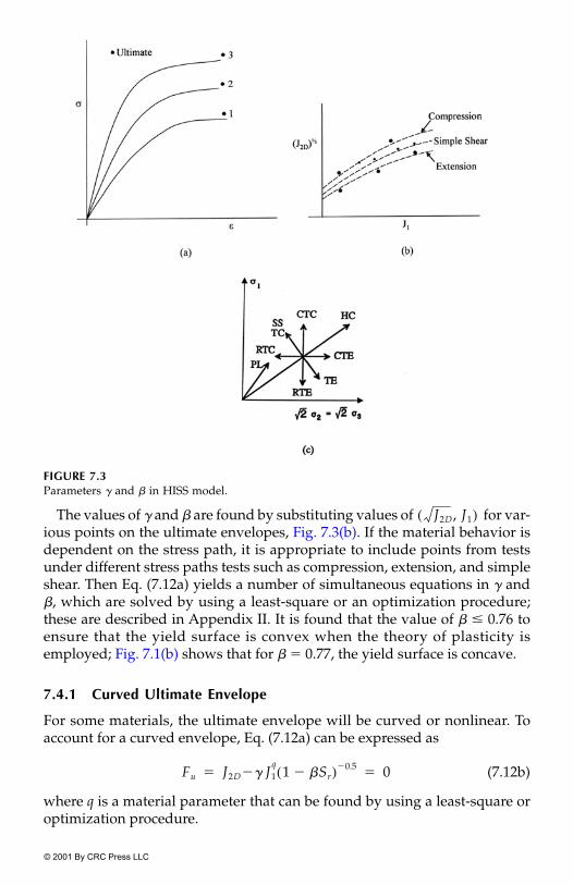
© 2001 By CRC Press LLC
The values of � and � are found by substituting values of for var-ious points on the ultimate envelopes, Fig. 7.3(b). If the material behavior isdependent on the stress path, it is appropriate to include points from testsunder different stress paths tests such as compression, extension, and simpleshear. Then Eq. (7.12a) yields a number of simultaneous equations in � and�, which are solved by using a least-square or an optimization procedure;these are described in Appendix II. It is found that the value of � � 0.76 toensure that the yield surface is convex when the theory of plasticity isemployed; Fig. 7.1(b) shows that for � � 0.77, the yield surface is concave.
7.4.1 Curved Ultimate Envelope
For some materials, the ultimate envelope will be curved or nonlinear. Toaccount for a curved envelope, Eq. (7.12a) can be expressed as
(7.12b)
where q is a material parameter that can be found by using a least-square oroptimization procedure.
FIGURE 7.3Parameters � and � in HISS model.
J2D, J1( )
Fu J2D � J1q
1 �Sr�( ) 0.5�� 0� �

© 2001 By CRC Press LLC
7.4.2 Relation Between Ultimate Parameters, Cohesion,and Angle of Friction
If the failure envelope in the Mohr–Coulomb criterion is assumed to be theultimate envelope, parameters � and � can be related to the traditional angleof friction, �, from the shear stress, �, vs. normal stress, , plots; see Fig 7.4.
FIGURE 7.4Ultimate envelopes in different stress spaces.

© 2001 By CRC Press LLC
The relations are given below (see Example 7.1 for derivations):
(7.13a)
(7.13b)
as Sr � 1 for compression (CTC) and Sr � �1 for extension (RTE) paths.Therefore,
(7.13c)
and
(7.13d)
Note that refers to the simple shear (SS) stress path, Fig. 7.3(b) and (c),when Sr � 0. In the foregoing equations �C, �S, and �E are the slopes of thecompression, simple shear, and extension envelopes in the �– stress space,and θC, θS, and θE are the corresponding slopes in the –J1 stress space,Fig. 7.4(a).
FIGURE 7.4(continued)
p1 �Ctan � 1 ��( )14---�
C
23
-------�Csin
3 �Csin�--------------------------
� � �
p2 �Etan � 1 ��( )14---�
E
23
-------�Esin
3 �Esin�--------------------------
� � �
��Ctan
1 ��( )0.5m---------------------------
�Etan
1 ��( )0.5m---------------------------� �
�p1
4 p24
�
p14 p2
4�
------------------�
�
J2D

© 2001 By CRC Press LLC
If � is constant, the ultimate envelope is a straight line. For some materials,the ultimate envelope is curved, and then � can be expressed as a function ofmean pressure (J1�3) as (33–36)
(7.14)
or
(7.15a)
or
(7.15b)
where �0 and �1 are parameters, and is the reference value. Thus, in thiscase, it is necessary to consider additional parameters in Eq. (7.14), which canbe found by using least-square fit procedures on plots of the ultimate enve-lope as a function of J1 (33, 36).
7.4.3 Bonding Stress, R
The bonding stress, R, is introduced by transforming the stress tensor as
(7.16)
where �ij is the Kronecker delta. In Fig. 7.1(a), 3R denotes the distance fromthe intersection of the ultimate yield surface with the J1-axis to the origin. Inthe case of geologic materials, where compressive behavior may be of the pri-mary interest, R is related to the tensile strength of the material. In the case ofmetals, where tensile behavior may be of the main interest, R is related to thecompressive strength.
The values of R can be obtained by assuming the ultimate envelope to be astraight line, from
(7.17)
where is the slope of the ultimate envelope and is proportional to thecohesive strength of the material.
� � J1( )�
� �0e�1 J1�
�
Fs
�1
�0----- J1
�Sr�exp
m
�
�0
ij� ij R�ij��
Rc
3 �----------�
� c

© 2001 By CRC Press LLC
The uniaxial tensile strength, ft (say for a concrete), can be used to evaluateR. As indicated in Fig. 7.4(c), the value of R is slightly greater than ft (33, 34,37):
(7.18)
For rocks, ft can be evaluated from the following empirical expression (38, 35,36), Fig. 7.4(d):
(7.19)
where fc is the uniaxial compressive strength, s � 1.0 for intact rock, and m� isfound from compression test results, which varies from about 0.001 forhighly disturbed rock masses to about 25 for hard, intact rock (38).
In the case of metals and metallic materials like solders, tensile behaviormay be relevant and the bonding stress, R, will represent (high) compressivestrength, as the ultimate yield envelope is essentially horizontal in the – J1 stress space; i.e., is small. For uniaxial tensile behavior, axial stress 1
is applied, for which J1 � 1 � 0 � 0 � 1 and At the ulti-mate yield condition [Fig. 7.1(a)]:
(7.20a)
(7.20b)
from which the value of � can be estimated. For example, we can assign asmall value of about 95% of at J1 � 0 and compute the slope , Fig7.1(a) (39, 40).
7.4.4 Phase or State Change Parameter
The phase change (PC) parameter, n, is related to the state of stress at whichthe material passes through the state of zero volume change. In the case ofmetallic materials that can be characterized as elastic perfectly plastic, theonset of the yield stress can represent the state of zero volume change, Fig. 7.5(a).
In the case of plastic hardening materials, such a state may occur duringthe hardening process, Fig. 7.5(b). For initially loose granular materials, it isapproached at higher deformations, Fig. 7.5(b). For initially dense materi-als, the state often is reached somewhere before the peak stress [point b, Fig.7.5(b)], at which the material experiences transition from compactive to
1.003 f t R 1.014 f t� �
f t12--- f c m� m�
2 4s��( )�
J2D
�J2D 1� 3( )1.�
J2Du
13
-------1u�
3RJ2Du
�------------- 1u��
J2Du�( )

© 2001 By CRC Press LLC
FIGURE 7.5 Stress-strain response and phase change or volume transition.

© 2001 By CRC Press LLC
dilative (volume increase) behavior. In the ultimate region, the state of zerovolume change is approached in the residual stress (critical-state) condition.The zero plastic volume change would occur when the volumetric plasticstrain increment vanishes, Fig. 7.5(c), that is, when 0. Based on Eq.(7.1), this leads to the expression for n as (1–6)
(7.21)
where the stresses are relevant to the point (from test data) where the volumechange is zero; Fig. 7.5(b) and (c). Details are given in Example 7.1.
The value of n can also be found from hydrostatic tests by using the follow-ing equation (4, 28, 41):
(7.22)
where dJ1 and d v are the increments in the J1 vs. v response, Fig. 7.5(d).The value of n should be greater than 2.0 for a convex yield surface and
may depend on such factors as initial density; however, as a simplification,an average value of n can be used. For dense granular materials like sands, nmay be around 3.0, while for loose granular materials and other materialssuch as rock and concrete, it would be higher, often of the order of 6 to 10.
For metallic materials and cohesive (saturated) soils, a value somewhathigher than 2, of the order of 2.05 to 2.40, is often found to be appropriate;such a value would imply a (nearly) elliptical yield surface. The followingprocedure may be used to evaluate n for cohesive materials. For these mate-rials, “failure” may occur long before the load along a stress path reaches the
FIGURE 7.5(continued)
�F� J1�( )�
n 2
1J2D
J12
-------- 1
Fs�---------�
------------------------------------
d v 0�
�
J1n�1 d v 3 n 2�( )� dJ1�

© 2001 By CRC Press LLC
ultimate envelope, Fig. 7.1(a). In other words, failure may occur when thephase change or the critical-state line, Fig. 7.5(e), is approached. Then thevalue of n is found from (28, 41)
(7.23a)
where J1m is the maximum value of J1 for a yield surface, and J1a is at the inter-section (A) of the phase change line and the yield surface. The value of J1m isfound from the effective consolidation pressure (p�) as
(7.23b)
The value of n can also be found from the slopes of the phase change line,�t, and the ultimate line (�) as
(7.24)
Details are given in Example 7.2.
7.4.5 Hardening or Growth Parameters
These parameters, e.g., a1 and �1 for � in (Eq. 7.11a), are found from labora-tory stress–strain tests plotted, for example, in terms of principal stresses, i
(i � 1, 2, 3), vs. principal strains i (i � 1, 2, 3); see Fig. 7.6(a). This implies thatthe test specimen is subjected to the principal stresses with no (applied) shearstresses. If the results are available from pure shear tests, then the plots interms of shear stress � and shear stress � can be used; see Fig. 7.6(b). The mainquantity needed here is the plastic strain trajectory given by
(7.25a)
or
(7.25b)
The increments of plastic strains , , or are found fromstress–strain curves, Fig. 7.6(a) or (b), based on the knowledge of the unload-ing modulus (Eu) or (Gu). Then, the increment of the trajectory d� is computedfor each stress increment and the total value � is found as
(7.26)
J1a
J1m-------
2n---
1
n�2------------
�
J1m 3p��
�t
�---- n 2�
n--------------
1� 2
�
� d 1p d 1
p d 2p d 2
p d 3p d 3
p��( )1�2��
� �D d�p d�
p( )1�2�� �
d 1p d 2
p d 3p d�
p
� �0 d�ii�1
j
���

© 2001 By CRC Press LLC
FIGURE 7.6Hardening or growth parameters, a1 and �1.

© 2001 By CRC Press LLC
where i is the increment and �0 is the initial value of � before the (shear) test.The latter denotes the plastic strains due to initial conditions such as initialstresses or strains (due to hydrostatic loading), microcracking, and defects. Ifthe material has no such prior history, �0 � 0.
Now Eq. (7.11a) is expressed as
(7.27)
The value of the hardening function, �, for the state of stress correspondingto the total stress after the stress increment, i, is found using Eq. (7.1), i.e., F � 0.Thus, values of ln� and ln� are found at various points along the stress-straincurves and are plotted as shown in Fig. 7.6(c). If the points are not widelyscattered, an average straight line is drawn through the points. The slope ofthe line gives �1, which denotes the rate of hardening. The intercept alongln�, when ln(�) � 0, i.e., � � 1, gives the value of a1. For some materials, thevalues of a1 and �1 may depend on factors such as initial density, stress path,and temperature. In that case, additional constants are needed to define a1
and �1. The values of parameters in other forms of �, Eq. (7.11), can beobtained similarly from laboratory test data (4–6, 19, 41).
7.4.6 Nonassociative �1-Model
The parameter � in Eq. (7.5) allows for the correction (deviation from normality)with respect to the �0-model; see Fig. 7.7(a). If it is assumed that the correctionis affected significantly by the volume change behavior, this parameter isobtained from the volumetric response, Fig. 7.7(b). In general, � can vary withstrain; however, as a simplification, it is assumed to be constant, related to theslope, Su, of the volumetric response near the ultimate region, Fig. 7.7(b).
FIGURE 7.6(continued)
� �1 �ln�ln a1ln�

© 2001 By CRC Press LLC
Then � is found from (4–6, 19, 20)
(7.28)
where Y and Z are related to the state of stress in the ultimate region and Su.The foregoing (eight) parameters (E, ν; �, �; n; a1, �1, and R) are required to
define the associative (isotropic hardening) �0-version in the HISS model. The�0-version can be used to characterize the behavior of material in the RI statein the DSC.
The introduction of the disturbance function, D, in the DSC, allows for thedeviation from normality of the observed strain increment, . In otherwords, the plastic strain increment from the �0-model is normal to F,while is not normal to F and shows deviation, �, from normality; Fig.7.7(a) (32). Such deviation can allow for the response as affected by frictionalcharacteristics, similar to that given by nonassociative plasticity models (19).Also, such deviation can represent a measure of induced anisotropy (26). Asa result, when the DSC model is used, it may not be necessary to employ theclassical nonassociative and anisotropic hardening models.
FIGURE 7.7Nonassociative response with DSC and parameter, �.
�1
�0 ��( ) 1 rv�( )------------------------------------------
YZ---- ��
�
d ˜
p a( )
d ˜
p i( )
d ˜
p a( )
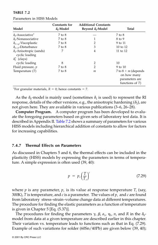
© 2001 By CRC Press LLC
As the �0-model is mainly used (sometimes �1 is used) to represent the RIresponse, details of the other versions, e.g., the anisotropic hardening (�2), arenot given here. They are available in various publications (3–6, 26–28).
Computer Program. A computer program has been developed to evalu-ate the foregoing parameters based on given sets of laboratory test data. It isdescribed in Appendix II. Table 7.2 shows a summary of parameters for variousHISS models including hierarchical addition of constants to allow for factorsfor increasing capabilities.
7.4.7 Thermal Effects on Parameters
As discussed in Chapters 5 and 6, the thermal effects can be included in theplasticity (HISS) models by expressing the parameters in terms of tempera-ture. A simple expression is often used (39, 40):
(7.29)
where p is any parameter, pr is its value at response temperature Tr (say,300K), T is temperature, and c is a parameter. The values of pr and c are foundfrom laboratory stress–strain–volume change data at different temperatures.The procedure for finding the elastic parameters as a function of temperatureis given in Chapter 5 [Eq. (5.37)].
The procedures for finding the parameters �, �, a1, �1, n, and R in the �0-model from data at a given temperature are described earlier in this chapter.Their variation vs. temperature leads to functions such as that in Eq. (7.29).Example of such variations for solder (60Sn/40Pb) are given below (39, 40);
TABLE 7.2
Parameters in HISS Models
ModelConstants for
�0-ModelAdditional Constants
Beyond �0-Model Total
�0-Associative� 7 to 8 — 7 to 8�0-Nonassociative 7 to 8 1 8 to 9�0�vp-Viscoplastic 7 to 8 2 9 to 11�0�D-Disturbance 7 to 8 3 10 to 12�2-Anisotropic (sands)
cyclic loading7 4 11 to 12
�0� (clays) cyclic loading 8 2 10
Fluid pressure, p 7 to 8 2 9 to 10Temperature (T) 7 to 8 m 7 to 8 � m (depends
on how many parameters are functions of T)
�For granular materials, R � 0; hence constants � 7.
p prTTr-----
c
�

© 2001 By CRC Press LLC
they are derived from uniaxial tension tests under two strain rates, �0.0002 and 0.002/sec (42); see Fig. 7.8.
Strain Rate � 0.0002:
(7.30a)
(7.30b)
Strain Rate � 0.002:
(7.31)
The value of � � 0 implies essentially a circular yield surface in the 1 – 2 – 3
space, and n � 2.1 is assumed for both strain rates. Variations for elasticparameters for the same solder are presented in Chapter 5.
7.4.8 Rate Effects
The responses of some materials are affected by the rate of loading. In thecontext of the laboratory behavior, the rate effect is often defined through thestrain rate, . The rate effect can be included in the HISS (and DSC) models
� T( ) �300T
300---------
0.072�
�300; 0.00082� �
� T( ) �300T
300---------
2.578�
�300;a1 300( )
�n1 300( )------------------� �
a1 300( ) 0.024 10�4�
�1 average( ); 0.394� �
R T( ) R300T
300---------
2.95�
R300; 217.5 mPa� �
E T( ) E300T
300---------
0.292�
E300; 23.45 GPa� �
� T( ) �300T
300---------
0.14
�300; 0.40� �
�1 T( ) �1 300( )T
300---------
0.24
�T 300( ); 3 10�6��K� �
� T( ) �300T
300---------
0.034�
�300; 0.00082� �
� T( ) �300T
300---------
5.5�
�300;a1 300( )
�n1 300( )------------------� �
a1 300( ) 2.0 �10 6��1 average( ); 0.615� �
R T( ) R300T
300---------
1.91�
R300; 240.67 MPa� �

© 2001 By CRC Press LLC
by expressing the parameters as functions of the rate. For example, for boththe thermal and rate effects, any parameter p can be expressed as
(7.32)
The parameters for appropriate functions in Eq. (7.32) can be determinedfrom laboratory tests under different T and . Strain rate effect is discussedlater in Chapter 8.
FIGURE 7.8Uniaxial tension stress–strain curves of 60% Sn–40% PB solders: (a) strain rate � 0.0002/sec,(b) strain rate � 0.002/sec (42). ©1990, IEEE. With permission.
p p T , ( )�

© 2001 By CRC Press LLC
7.5 Repetitive Loading
Under repetitive loading, Fig. 7.9(a), the applied load amplitude is increased(to P0) and decreased to zero, and then increased to P0 after a lapse of time,�t. If we ignore, for the time being, the effect of time, we can consider that theload is applied as above repeatedly at different cycles, N, and the behavior ofthe material may be assumed to be independent of time.
Under the application of the external load, P0 , a material element wouldundergo loading–unloading–reloading cycles as depicted in Fig. 7.9(b). Here,upon removal of the load, P0, the state of stress in a material element, may notreturn to zero. In other words, at the end of unloading in a given cycle, thematerial may retain a residual or initial stress, , Fig. 7.9(b).
FIGURE 7.9Repetitive load and stress conditions.
˜ r N( )

© 2001 By CRC Press LLC
Figure 7.9(c) depicts the situation with respect to yield surfaces in theJ1– space. Loading from 0 to A starts from the initial state , and atthe end of the loading, the state will be . Upon unloading, (A–B),during which plastic-strain change may occur, the state will be . Thenreloading to P0 (B–C) will start from the residual or initial state ; ingeneral, the residual state will be , where N is the cycle num-ber. Thus, the application of full load P0 will start from the residual condition,which can be considered as the initial state for the current cycle, and willresult in the modified matrix, , corresponding to the residual state. Hence,repetitive loading will lead to continuously increasing plastic strains as thecycles increase. However, the rate of increase in plastic strains may decreasewith cycles.
The foregoing approach can be used to simulate behavior of materials(metals, geologic, asphalt, etc.) under repetitive loading. When implementedin a computer (finite-element) method, the procedure would allow calcula-tion of displacements, stresses, strain, and pore water pressures under repet-itive loading (see Chapter 13). Examples of materials such as asphalt andsoils, with simplified procedures for computing plastic or permanent strains(deformations), are given later.
7.5.1 Dynamic Loading
Implementation of the HISS and DSC models for dynamic (earthquake) anal-ysis is given in Chapter 13. Here, the loading and the stress–strain behaviorcan involve both positive and negative values of loads and stresses, which isoften referred to as two-way loading; see Fig. 7.10.
7.6 The Derivation of Elastoplastic Equations
The total (incremental) strain, , is decomposed and expressed in matrixnotation as
(7.33)
where � elastic strain vector, and � plastic strain vector.The incremental elastic strain, , is related to the increment stresses, ,
as
(7.34)
J2D ˜ 0, �0( )
˜ A, �A( )
˜ B, �B( )
˜ B, �B( )
˜ r N( ), �r N( )[ ]
C˜
ep
d ˜
i
d ˜
i d ˜
e d ˜
p��
d ˜
e d ˜
p
d ˜
e d˜
d˜
C˜
e d ˜
e�

© 2001 By CRC Press LLC
Here, the elastic constitutive matrix, , for isotropic material is expressedin terms of the elastic modulus, E, and Poisson’s ratio, �, or the shear modu-lus, G, and the bulk modulus, K. Often, these parameters are assumed to beconstant for all increments during the incremental analysis. However, theycan be considered as variable and expressed as tangent quantities:
(7.35)
or
(7.36)
where the subscript t denotes tangent quantity, which can be found as thederivative (slope) of the function used. The latter can be such mathematicalfunctions as hyperbola, parabola, splines, and exponential (43).
FIGURE 7.10Dynamic loading.
C˜
e
Et Et 1 3�( ), p[ ] and �t �t 1 3�( ), p[ ]��
Gt Gt J2D, J1( ) and Kt Kt J1, J2D( )��

© 2001 By CRC Press LLC
Now, from the theory of plasticity, we can use the normality rule (44, 45)
(7.37)
and the consistency condition as
(7.38)
where � vector of incremental plastic strains, and � is a scalar (positive)proportionality parameter.
Equation (7.38) gives
(7.39)
The term d� is given by
(7.40)
Therefore, Eq. (7.39) leads to
(7.41)
Substitution for from Eq. (7.34) gives
(7.42a)
and substitution for from Eq. (7.33) leads to
(7.42b)
d ˜
p�
�Q�
˜
--------�
dF 0�
d ˜
p
�F�
˜
-------
T
d˜
�F��------ d�� 0�
d� d ˜
p( )Td
˜
p
1�2
�
��Q�
˜
--------
T
��Q�
˜
--------
1�2
�
��Q�
˜
--------
T �Q�
˜
--------
1�2
�
��F�
�F�
˜
-------
T
d˜
�F��------ � �F � 0�
d˜
�F�
˜
-------
T
C˜
e d ˜
e �F��------ � �F � 0�
d ˜
e
�F�
˜
-------
T
C˜
e d ˜ � d
˜p( ) �F
��------ � �F � 0�

© 2001 By CRC Press LLC
which, with from Eq. (7.37), gives
(7.42c)
Hence,
(7.42d)
which leads to the expression for � as
(7.43)
Now, use of Eq. (7.37) with � and substitution in Eq. (7.34) gives
(7.44a)
(7.44b)
or
(7.44c)
(7.44d)
Here, is called the elasto-plastic constitutive matrix.Note that for associative plasticity, Q � F will be substituted in Eq. (7.44), and
that Eq. (7.44) can be used for any F and Q, including those from Chapter 6 andEqs. (7.1) and (7.4).
d ˜
p
�F�
˜
-------
T
C˜
ed ˜ �
�F�
˜
-------
T
C˜
e�
�Q�
˜
-------- �F��------� � �F 0�
�F�
˜
-------
T
C˜
e d ˜
� �F�
˜
-------
T
C˜
e �Q�
˜
-------- �F��
˜
------ �F�� 0�
�
�F�
˜
------- T
C˜
e d ˜
�F�
˜
------- T
C˜
e �Q�
˜
-------- �F��
˜
------ �F�
-------------------------------------------------------�
d˜
C˜
e d ˜
d ˜
p�( )�
C˜
eC˜
e �Q�
˜
-------- �F�
˜
------- T
C˜
e
�F�
˜
------- T
C˜
e �Q�
˜
-------- �F��------ �F�
------------------------------------------------------� d ˜
�
d˜
C˜
e C˜
p�( )d
˜�
d˜
C˜
ep d ˜
�
C˜
ep

© 2001 By CRC Press LLC
7.6.1 Details of Derivatives
We now give details of the derivatives involved in Eq. (7.44). The quantities and will be used as J1 and J2D (without overbars) with the understand-
ing that they are nondimensionalized with respect to pa; hence, although notshown in the following derivations, pa will occur in the denominator.
From the chain rule of differentiation, we have from Eq. (7.1)
(7.45a)
where
(7.46a)
and
(7.47b)
(7.47a)
Here
(7.47b)
where Sij is the deviatoric stress tensor:
(7.47c)
(7.48a)
and
(7.48b)
where Tij � Sik Skj.
J1 J2D
�F J1, J2D, J3D( )�ij
---------------------------------------�F�J1-------
�J1
�ij---------
�F�J2D-----------
�J2D
�ij----------- �F
�J3D-----------
�J3D
�ij-----------���
�F�J1------- n�J1
n�1 2�J1�( )Fs�
�J1
�ij--------- �ij or �J1
�˜
-------
T
1 1 1 0 0 0� �
�F�J2D----------- 1 Fb m 1 �Sr�( )m�1[ ] �
32---
272
---------- J3D J2D5�2�
��
�J2D
�ij----------- Sij�
Sij ij
J1
3---- �ij��
�F�J3D----------- m�
272
----------Fb 1 �Sr�( )m�1 J2D3�2�
�
�J3D
�ij----------- Tij
23--- J2D �ij��

© 2001 By CRC Press LLC
The above expressions can be written in the matrix notation, e.g., Eq.(7.47b), as
(7.47c)
where = [S1 S2 S3 S4 S5 S6] � [S11 S22 S33 2S12 2S23 2S31] denote the componentsof the deviatoric stresses, and Eq. (7.48b)
(7.48c)
where � [T1 T2 T3 T4 T5 T6] � [T11 T22 T33 2T12 2T23 2T31].The expressions for and can be calculated
similarly. The main difference will be in the expression of �, i.e.,
For the �0-msodel:
(7.49a)
For the �1-model:
(7.49b)
where �Q is given in Eq. (7.5).
7.7 Incremental Iterative Analysis
The verification of a constitutive model constitutes an important phasetoward reliable use of the model for practical application. Such verification isusually performed in two steps: (1) prediction of laboratory tests for whichthe parameters are determined and of independent tests not used in finding
�J2D
�˜
-----------
T
S˜
T�
S˜
�J3D
�˜
-----------
T
T123--- J2D�
T223--- J2D�
T323--- J2D�
T4
T5
T6
�
T˜
T
�Q��J1, �Q��J2D, �Q��J3D
Fb0 ��J1n
�J12
��
Fb1 ��QJ1n
�J12
��

© 2001 By CRC Press LLC
the parameters; and (2) implementation of the model in solution (computerfinite-element) procedures and then prediction of the behavior of practical(field) boundary-value problems and�or those simulated in the laboratory. Inthis chapter, we present details of the implementation of the HISS model incomputational procedures, and validations with respect to laboratory behav-ior of a number of materials. Validations with respect to (field) boundary-value problems are given in Chapter 13.
In dealing with nonlinear material behavior, e.g., elastoplastic characteriza-tion, it is usually necessary to perform incremental analysis, very oftenaccompanied by iterations so as to ensure convergence to equilibrium states.The finite-element incremental equations in the displacement-based approachare derived as (46)
(7.50)
where � tangent stiffness matrix, � vector of nodal displacements, �vector of nodal-applied loads, d denotes increment, and i denotes incrementalstage of loading. Here, the total load is divided into (small) increments �
; see Fig. 7.11(a); the number of increments, N, is chosen by the analyst,depending on the properties of the problems on hand and experience. Thestiffness matrix is given by
(7.51)
where V is the volume (of finite element) and is the strain-displacementtransformation matrix in (46, 47)
(7.52)
� vector of strain components. Note that in Eq. (7.51) the elastoplastic con-stitutive matrix is evaluated at the start of the current increment (i) or at theend of the previous increment (i � 1); Fig. 7.11(b).
The assembled equations are solved for incremental displacements at allnode points, which provides the incremental element strains from Eq. (7.52).Then the incremental stress, is evaluated from
(7.53a)
and the total stress after the increment is given as
(7.53b)
k˜
d q˜
idQ
˜i�
k˜
q˜
Q˜
Q˜dQ
˜i
k˜
k˜ i�1 B
˜TC
˜ i�1ep B
˜Vd��
B˜
d ˜ i
B˜
dqi�
˜
d˜
d˜ i Ci�1
ep d ˜ i
�
˜ i
˜ i�1 d˜ i��
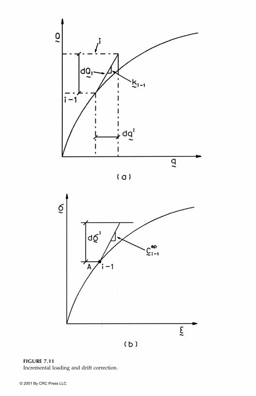
© 2001 By CRC Press LLC
FIGURE 7.11Incremental loading and drift correction.

© 2001 By CRC Press LLC
Now, if (by chance) the stress, , and the corresponding hardening func-tion, �i, after the stress increment, , satisfy the yield function, F, at point B[Fig. 7.11(c)], then
(7.54)
Here, � and �B � hardening function at B (see below). However, such anoccurrence is rare, and usually Eq. (7.54) will not be satisfied. The “correct” yield sur-face F, shown by the dashed curve in Fig. 7.11(c), will, therefore, be different from ;the difference between them is often referred to as the drift. Hence, it becomes neces-sary to correct for the drift so as to obtain F ≈ 0. This process is called drift correction.
FIGURE 7.11(continued)
˜ i
d˜ i
F ˜ B, �B( ) 0�
˜ B
˜ i
F

© 2001 By CRC Press LLC
7.7.1 Possible Stress States
The above case, i.e., when point A is exactly on the previous yield surface at(i � 1), may not occur for all Gauss points (elements). In other words, at (i � 1)some points may be in the elastic range, as indicated by in Fig. 7.11(c).In the case of incremental analysis, it becomes necessary to consider bothpossibilities.
In order to check whether or not the current surface F � 0 is satisfied, weneed to calculate the hardening function, �, Eq. (7.11). This is achieved by cal-culating the plastic strain increment as
(7.55)
in which the elastic strains vector, , is obtained from
(7.56)
Once is found, the total plastic strain trajectory [Eq. (7.26)] is found as
(7.57)
Then, �i is found from Eq. (7.11).Now, and �i are substituted in Eq. (7.1) as
(7.58)
If F � 0, then the new stress point lies on the corresponding yield surface,and we proceed to the next increment.
Elastic State. If F � 0, the new stress point is in the elastic (unloading)region; and if F � 0, (drift) correction is needed. For elastic unloading [A toA2 or to Fig. 7.11(c)], assuming that during unloading, no plasticstrains occur (i.e., �A remains the same), the total stress is found as
(7.59)
7.7.2 Elastic-Plastic Loading
If F � 0, i.e., there is elastoplastic loading, two cases need consideration.Case 1. The material is in the elastic range at the start of the current incre-
ment and yields during this increment, to ; Fig. 7.11(c). Since the behavioris elastic from to C, it is necessary to calculate the stress state at C so as to
A
d ˜ i
p d ˜ i
d ˜ i
e��
d ˜ i
e
d ˜ i
e C˜
e( ) 1�d
˜ i�
d ˜ i
p
�i �i�1 d ˜ i
p( )Td
˜ ip[ ]
1�2��
˜ i
F ˜ i, �i( ) �
�----- 0
A A2,
˜ i
˜ i�1 C˜
e d ˜ i��
A BA

© 2001 By CRC Press LLC
apply the drift correction scheme for C to . Here, a Newton–Raphson-typeprocedure can be used to find, iteratively, from iterations (j � 1, 2, . . . , m) thefraction of the stress increment that provides the location of point C. For this,we write the yield surface, F, as
(7.60)
Therefore,
(7.61)
which represents the portion of the total stress increment that represents thecorrection to locate the stress state at point C. Then the stress at the jth itera-tion is given by
(7.62)
Here, � . The iterations j are continued until convergence is reached.For instance, the convergence is considered to have been reached when
(7.63)
where is the tolerance, which can be equal to (or less).Now, the actual strain increment, from C to , is computed as the strain
increment, minus the elastic strain increment from to C, i.e.,
(7.64)
With the above information, we have the stress at point C �and the stress at point (or B) � ; and the strain increment from C to
. Now we can apply the correction so as to locate F � 0 at point D, Fig. 7.11(c).Case 2. Here, the increment starts at point A when FA � 0, which is a spe-
cialization of case 1.
7.7.3 Correction Procedures
A number of correction procedures have been proposed in the context of theincremental-iterative analysis for the integration of elastoplastic equations,e.g., subincrementation (2, 28, 48), drift correction (49, 28), and substepping
B
F ˜ i�1
j�1�
jd˜ i, � i�1
j�1�( )[ ] F
˜ i�1j�1, �i�1
j�1( ) �j �F�
˜
------- d˜ i� 0� �
�j F
˜ i�1j�1, �i�1
j�1( )�F�
˜
------- d˜ i
---------------------------------��
i�1j
i�1j�1
�jd
˜ i��
˜ i�1
0˜ i�1
F i�1j , �i�1( ) �
10 4�
d ˜
j Bd
˜A
d ˜
d ˜ i
�j
j� C
˜e( ) 1�
d˜ i��
˜ i�1
j˜ i�1�
B ˜ i d
˜i
B

© 2001 By CRC Press LLC
(50). The subincrementation procedure may lead to convergence if the subin-crements (of strain) are adopted to be very small. It can be appropriate forintegrating the incremental constitutive equations, Eq. (7.44), for backpre-dicting stress–strain responses. However, when the finite-element analysis,with many elements, is to be performed, the subincrementation procedurecan be time-consuming and may not often provide convergence. In that case,the drift correction based on predictor-correction procedures, often in combi-nation with the subincrementation procedure, can provide improved androbust schemes. In the substepping scheme, the stress increments are com-puted on the basis of known strain increments by adjusting the size of eachsubstep automatically (50). The subincrementation and drift correction pro-cedures are used commonly with the HISS-plasticity models. Hence, theirdetails are given below.
7.7.4 Subincrementation Procedure
It is first required to set initial values of various quantities as
(7.65)
Here the strain increment corresponding to C to (or A to B) is divided intoa number of small strain increments � �n, where n is the numberof subincrements, Fig. 7.11(c).
For each subincrement, say the mth, the total stress is computed as
(7.66)
and the corresponding hardening parameter, is found by computing thetrajectory, as
(7.67)
where
and � is computed using Eq. (7.43).Now check if F � tolerance. If the subincrement is small (and if the
tolerance is satisfied), we consider the subincremental results satisfactoryand proceed to the next subincrement. If the subincrement is large and theabove criterion is not satisfied, it is possible to perform the drift correction
˜ i
0˜ i�1; C
˜ iep 0( ) C
˜ i�1ep
� �i0
�i�1� �
B� d
˜ i( ) d
˜ ij
˜ i
m˜ i
m�1 C˜ i
ep m�1( )� d
˜ i( )��
�ij,
�ij,
�im
�im�1
� d�( )��
d� ��Q�
˜
--------
T �Q�
˜
--------1�2
�
im, �i
m( )

© 2001 By CRC Press LLC
(described below) for the current subincrement so as to improve the accuracy,before going to the next strain subincrement (m � 1).
For the next subincrement, compute the constitutive matrix, , usingEq. (7.44). Then apply the next subincrement, and go to Eq. (7.66).When all subincrements are applied, Fig. 7.11(c),
(7.68)
In the case of the integration of the incremental equations for back predic-tions of stress–strain responses, it may be necessary to perform the aboveprocedure only once before proceeding to the next increment. However, forfinite-element analysis, it needs to be performed for all Gauss points in theelements, and the quantities in Eq. (7.68) are stored for all such points beforeproceeding to the next (load) increment.
7.8 Drift Correction Procedure
A drift correction procedure can be used by itself or together with the subin-cremental strain scheme described earlier. It is believed that the drift correc-tion procedures are needed in finite-element analysis with most nonlinear(plasticity) models.
Assume that for both cases 1 and 2, the yield surface at the start (at C or A)is satisfied [Fig. 7.11(c)], i.e.,
(7.69)
Now, the current increment, i, causes the stress increment, , which takesus to point B [Fig. 7.11(c)], at which is not satisfied. The yieldsurface condition is satisfied at the (desired) point D, where F � 0.Hence, the drift correction procedure would entail modifications in and
so as to lead to .The quantities at point B are found as follows:
(7.70a)
where
(7.70b)
(7.71a)
Ciep( )m
� d ˜ i
( ),
˜ i i
n; C˜ i
ep C˜ i
ep( )n; �i �i
n; and �i �in
� � � �
F ˜ A, �A( ) 0�
d˜
B
F ˜ B, �B( ) 0�
˜ D, �D( )
˜ B
�˜ B
˜ D, �˜ D
˜ B
˜ A d˜ i( )A�B��
d˜ i( )A�B C
˜e d
˜e( )
A�B�
�B �A d�A�B��

© 2001 By CRC Press LLC
(7.71b)
(7.71c)
Here, � � and is found using Eq. (7.52).Now let the errors or modification required in the elastic and plastic incremen-
tal strains be denoted as and Then [Fig. 7.11(d)], respectively.
(7.72)
Considering that the strain increment � � is the same atpoint D [Fig. 7.11(d)], we have
(7.73a)
Therefore,
(7.73b)
In other words, the plastic strains from B � D are accompanied by an equaldecrease in the elastic strains.
Then, at the converged state, D, we have
(7.74a)
where
(7.74b)
and the hardening parameters are
(7.75a)
where
(7.75b)
where the functions f1 and f2 will depend on the hardening function used, e.g.,Eq. (7.11).
d�A�B d ˜
p( )Td
˜p
1�2
�
f 1 d ˜
p( )�
�B
a1
�B�1
------ f 2 �( )� �
d ˜
p d ˜
d ˜
e d ˜
d ˜
e( )BD
d ˜
p( )BD
.
d ˜ i
d ˜ AB
e d ˜ AB
p d ˜ BD
e d ˜ BD
p� � ��
d ˜ i
d ˜ AB
e d ˜ AB
p
d ˜ BD
e d ˜ BD
p� 0�
d ˜ B�D
e d B�Dp
��
˜ D
˜ B d˜ BD��
d˜ BD C
˜e d
˜BDe
�
�D �B d�BD��
d�B�D f 1 d ˜
p( )BD
� and �D f 2 �( )D�

© 2001 By CRC Press LLC
Substitution of Eqs. (7.74a), (7.75a), and (7.75c) in the equation for F gives
(7.76)
which, when expanded into the Taylor series, gives
(7.77)
Now, from the normality rule,
(7.78)
Here, Q ≡ F for associated plasticity.Substitution of Eq. (7.78) into (7.75b) gives
(7.79)
Substitution of Eqs. (7.73b) and (7.78) into Eq. (7.74b) gives
(7.80)
Now, substitution of Eqs. (7.79) and (7.80) into Eq. (7.77) gives
(7.81)
Ignoring higher-order terms, we find the expression for �BD as
(7.82)
F ˜ B d
˜ BD�( ) f 2 �B d�BD�( ),[ ] 0�
F ˜ B, f 2 �( )B
�F�
˜
-------
T
d˜ B�D
�F� f 2--------
d f 2�B
…� � 0�
d ˜ BD
p�BD
�Q�
˜
--------
B
�
d�BD �BD f 1�Q�
˜
-------- �
d˜ BD �BD C
˜e�Q�
˜
--------��
F ˜ B, f 2 �( )B �
�F�
˜
-------
B
T
C˜
e�Q�
˜
-------- �F��-------
� f 2
��--------
B
f 1�Q�
˜
--------�
B
�B�D…� � 0�
�BD
F ˜ B, f 2 �( )B[ ]�
� �F�
˜
-------
B
TC˜
e�Q�
˜
--------�F��-------
� f 2
��---------
B
f 1�Q�
˜
--------� -------------------------------------------------------------------------------------------�

© 2001 By CRC Press LLC
Hence, the quantities at D can be found as
(7.83a)
(7.83b)
and
(7.83c)
Hence,
(7.84)
should be satisfied, for a given tolerance to Then, Eq. (7.84) willrepresent the converged yield surface for increment i.
As the higher-order terms in Eq. (7.81) are ignored, it may be appropriateand sometimes required to perform iterations using the result in Eq. (7.82).Here, the solutions obtained in Eq. (7.83) can be substituted in Eq. (7.82), andthe next set of the quantities are calculated. The procedure is continued untilEq. (7.84) is satisfied.
7.9 Thermoplasticity
The temperature effects in the plasticity model can be introduced through themodification of various terms. For example, the yield function in the HISS (�0)model can be expressed as (39, 40)
(7.85)
where T is the temperature, � J1 � 3R, R(T) is the bonding stress; here, theinvariant quantities denote nondimensionalized values with respect to pa.The temperature-dependent hardening function, �, can be written as
(7.86)
˜ D
˜ B �BD C˜
e �Q�
˜
--------��
�D �B �BD f 1�Q�
˜
-------- ��
�D f 2 �( )D�
F ˜ D, �D( ) 0�
10 3�( 10 6� ).
F T( ) J2D � T( )J1n T( )
� T( )J12
��[ ] 1 � T( )Sr�[ ] 0.5�� 0� �
J1
� T( )a1
��1
------�

© 2001 By CRC Press LLC
where a1 and �1 are hardening parameters that may be expressed as functionsof T, and � is the thermoplastic strain trajectory. Depending on the effect oftemperature, a1 and�or �1 may be essentially constant with temperature.
The normality rule can now be used (51, 52):
(7.87)
The total incremental strain vector can be decomposed as
(7.88)
where is the strain vector due to the temperature change, dT. Hence,
(7.89)
and
(7.90)
where � [1 1 0] and [1 1 1 0 0 0] for two-dimensional andthree-dimensional cases, respectively.
Now the consistency condition gives
(7.91)
Therefore,
(7.92)
The use of Eqs. (7.89), (7.90), and (7.91) leads to the expression of � as
(7.93)
d ˜
p T( ) ��Q
˜, �, T( )
�˜
------------------------------�
d ˜
t T( )
d ˜
t T( ) d ˜
e T( ) d ˜
p T( ) d ˜
T( )� ��
d ˜
T( )
d ˜
e T( ) d ˜
t�
�Q�
˜
-------- d ˜
T( )���
d˜
C˜
e T( )d ˜
e�
C˜
e T( ) d ˜
t�
�Q�
˜
-------- �TI˜0 dT���
I˜0
dF ˜
, �, T( ) 0�
dF �F�
˜
-------
T
d˜
�F��------ d�
�F�T------- dT���
�
�F�
˜
------- T
C˜
e T( )d ˜
�F�T-------dT �T
�F�
˜
-------C˜
e T( )I˜0 dT��
�F�
˜
-------C˜
e T( )�Q�
˜
-------- �F��------ �Q
�˜
-------- T �Q
�˜
--------1�2
�
---------------------------------------------------------------------------------------------------------�

© 2001 By CRC Press LLC
Substitution of � in Eq. (7.90) gives
(7.94a)
(7.94b)
where is the unit matrix.Material Parameters. The variation of the elasticity and plasticity param-
eters and �T is shown in Eq. (7.29). Their determination has been discussedearlier in Section 7.4.7, “Thermal Effects on Parameters.”
7.10 Examples
We now present examples of derivations and properties of some of theexpressions in the HISS models, analysis of the effect of stress paths, and val-idation of the models with respect to the laboratory test behavior of a numberof materials.
Example 7.1Derive the conditions on parameters n, �, and � in the yield function, F ofEq. (7.1).
Parameter n:The state when the volume transits from compaction to dilation, or change involume vanishes, i.e., d v � 0, is related to the highest point on the yield sur-face (Fig. 7.1), where � 0:
(1a)
, Fs, and � refer to the state of stress at the transition. Equation (1a) leads to(as Fs ≠ 0)
(1b)
d˜
C˜
e T( ) I˜
�
�Q�
˜
--------�F�
˜
------- T
C˜
e T( )
�F�
˜
------- T
C˜
e T( )�Q�
˜
-------- �F��------ �Q
�˜
-------- T �Q
�˜
--------1�2
�
------------------------------------------------------------------------------------- d ˜
�
C˜
e� T( ) �TI
˜0 �
�T�F�
˜
-------C˜
e T( ) I˜0
�Q�
˜
-------- �F�T-------
�Q�
˜
--------�
�F�
˜
------- T
C˜
e T( )�Q�
˜
-------- �F��------
�Q�
˜
-------- T �Q
�˜
--------1�2
�
-------------------------------------------------------------------------------- dT
C˜
ep T( )d ˜
d˜
T( )��
I˜
T
�F��J1
�F�J1
------- �nJ1n�1
2�J1�( )Fs 0��
J1
J1( )t2�
�t n-------------
1
n�2------------
�

© 2001 By CRC Press LLC
where the subscript t denotes transition. Now Eq. (7.1) at the transitionbecomes
(1c)
Substitution of Eq. (1b) in Eq. (1c) leads to
(1d)
Because Fs and�t are positive, the term in the brackets should be nonnegative.Therefore, n � 2.
Alternatively, for � � 0, Eq. (7.1) gives
(1e)
The curvature, �, of the projection surface (curve) in Eq. (1e) can beexpressed as
(1f)
For the yield curve to be convex, � � 0. Solution of Eq. (1f) numerically leadsto the condition that n � 2 (53).
Parameter � :At the ultimate condition, � � 0. Therefore, from Eq. (7.1) we have
(1g)
As � 0 and � 0, and as � � 1 (see below), � 0. Hence,� � 0.
Now for hydrostatic or spherical state of stress, J2D � 0 and Eq. (7.1) gives
(1h)
when � � 0, as � � 0, � �. That is, the ultimate envelopes intersect with
J2D( )t �t J1( )tn
� � J1( )2� Fst�
J2D
J12
-------
t
�t �2�n
------� Fst� �
J2D �J1n
� �J12
�( ) 0.5��
�
�2 J2D
� J12
-----------------
1� J2D
� J1---------------
2
�
3�2----------------------------------------�
J2D
J12
------- � 1 �Sr�( ) 0.5��Fs� �
J2D J12
1 �Sr�( ) 0.5�
��--- J1( )n�2
�
J1

© 2001 By CRC Press LLC
the J1-axis at infinity. For � � 0, the yield surface (Fig. 7.1) will intersect theJ1-axis at finite values. For � � ∞, the state of stress will be at � 0.
Parameter � :The slope (�) of an ultimate envelope [Fig. 7.4(a)] is given by
(1i)
For Fs � 1 when Sr � 0, i.e., for the simple shear (S) stress path, � �.For other stress paths, i.e., Sr � !1 (Sr � 1 for compression and � �1 forextension paths):
(1j)
or
(1k)
If � � 0, � �. If � � 1, Eq. (1j) gives � 0, which is inadmissible.If � � 1, (1 � �) in Eq. (1j) would give a negative value, which is not admis-sible. Hence, 0 � � � 1.
Alternatively, from Eq. (7.1) we have
(1l)
where C1 � � � � constant. On the "-plane in the principal stressspace (Fig. 7.12), we have (53)
(1m)
where Si (i � 1, 2, 3) are the normal components of the deviatoric stress tensor,Sij; x, and y are the Cartesian coordinates; and r is the radius of the polar coor-dinate system. Then Eq. (1m) leads to
(1n)
J1
2tan �J2D
J12
------- �Fs � 1 �Sr�( ) 0.5�� � �
tan2�
2tan �C � 1 ��( ) 0.5��
2tan �E � 1 ��( ) 0.5��
2tan � 2tan �
J2D C1 1272
----------J2D
J2D3�2
------- � �
0.5�
�
� J1( )nJ1
2( )
r2 2J2D�
yi Si�
�iyi
r----�
r 2C1 1 � 3�sin�( ) 0.25��

© 2001 By CRC Press LLC
For the yield surface to be convex, � should be such that the curvature, � � 0,
(1o)
The numerical solution of Eq. (1o) shows that
Example 7.2 Derive Eq. (7.24)At point B [Fig. 7.5(e)] J2D � 0. Assuming Sr � 0, we have, from Eq. (7.1),
(2a)
Therefore,
(2b)
Now, the use of Eq. (1b) in Eq. (2b) gives
(2c)
where J1a is related to the phase change point A [Fig. 7.5(e)].At the ultimate condition, � � 0; therefore, Eq. (7.1) leads to
(2d)
FIGURE 7.12Plot on "-phase (53).
�2r�
2 2rr#� r2�
r�2 r2
�( )3�2-----------------------------------------�
0 � 0.755923.��
�J1m
n
pan
-------�J1m
2
pa2
-----------�
J1m
pa------- �
�---
1
n�2------------
�
J1a
J1m------- 2
n---
1
n�2------------
�
�J2D
J1----------- �Fs� �

© 2001 By CRC Press LLC
where � is the slope of the ultimate line [Fig. 7.5(e)]. Equation (7.1) can bewritten as
(2e)
Now, substitution of Eq. (1b) at the transition state in Eq. (2e) gives
(2f)
where �t is the slope of the phase change line [Fig. 7.5(e)]. Therefore,
(2g)
Example 7.3Derive the relations between the slopes (compression and extension) in theJ1– and �– (Mohr–Coulomb) stress spaces.
It is useful to derive the relations (Eq. 7.13) between the slope of the ultimatesurface and [Fig. 7.4(a)], the traditional slope (�) of the failureenvelope in the Mohr–Coulomb criterion [Fig. 7.4(b)]. Then, � can be com-puted from the angle of friction, �.
First consider compression path. From Fig. 7.4(b), we have
(3a)
At the ultimate condition, � � 0; therefore,
(3b)
Now, by substituting 2 � 3, we have
J2D
J12
------- �J1
n�2
pan�2
----------� ��
Fs� 0�
�t
J2D
J1----------- 1
2n---�
� Fs
1�2
� �
�t
�----
n 2�n
--------------
1�2
�
J2D
� �Fs�( )
1 3�
1 3�------------------- �sin�
J2D
J1----------- � 1 �Sr�( ) 0.5�
�
J2D16--- 2 1 3�( )2 and J1 1 23�� �

© 2001 By CRC Press LLC
Therefore,
(3c)
Then Eqs. (3a), (3c), and (3d) give
(3d)
where is the slope of the ultimate envelope [Fig. 7.4(a)].Similarly, for the extension path,
(3e)
7.11 Stress Path
The behavior of most materials is influenced by the path of loading or stresspath. The stress paths are usually depicted on stress spaces such as J1– ,1– 1–2, and 1–2–3. In the case of materials such as metalsand alloys, tensile loading is often more significant. Here, tension is consid-ered to be positive. Figure 7.13(a) shows uniaxial tension and compressiontest (1 $ 0, 2 � 3 � 0) and a schematic of stress–strain responses. The stresspath followed during the uniaxial tension (UT0) and uniaxial compression(UC0) tests are depicted in three stress spaces [Fig. 7.13(a)]. In the J1–space, the stress path has the slope of
In the 1–2 space, the stress paths are vertical. In the 1–2–3 space, thestress paths follow the 1-axis.
Figure 7.13(b) shows straight-line stress paths used commonly for fric-tional (geologic) materials. Often, other stress paths such as proportionalloading (PL) and circular (CSP) are followed. The latter can capture the com-bined effect of a number of stress paths in a single test. Table 7.3 shows an
J2D
J1----------- 1
3-------
1 3�
1 23�---------------------- 1
3-------
1 3�
1 3�( ) 3�--------------------------------------� �
13
-------1 3�( )� 1 3�( )1 3 � 1 3�( )�
---------------------------------------------------�
�CtanJ2D
J1----------- 2
3-------
�csin3 �csin�-------------------------� �
�c � 1 �Sr�( ) 0.5��
�Etan � 1 �Sr�( ) 0.5� 23
-------�Esin
3 �Esin�--------------------------� �
J2D
22 � 23( ),
J2D
1� 3 J2D�J113
-------1
1-----�

© 2001 By CRC Press LLC
explanation of various stress paths and their loading conditions in terms ofprincipal stresses, 1, 2, and 3.
7.11.1 Stress Path Analysis of the HISS Model
Material points in any engineering structure may experience changes inthe stress paths during loading, unloading, and reloading. For instance, duringincreasing load, a point may follow the compression stress (CTC) path[Fig. 7.13(b)]; however, upon unloading, it may follow the opposite path
FIGURE 7.13Stress paths in testing.
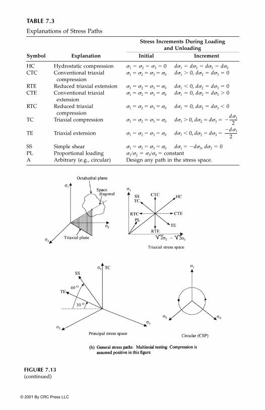
© 2001 By CRC Press LLC
TABLE 7.3
Explanations of Stress Paths
Stress Increments During Loadingand Unloading
Symbol Explanation Initial Increment
HC Hydrostatic compression 1 � 2 � 3 � 0 d1 � d2 � d3 � d0
CTC Conventional triaxial compression
1 � 2 � 3 � 0 d1 � 0, d2 � d3 � 0
RTE Reduced triaxial extension 1 � 2 � 3 � 0 d1 � 0, d2 � d3 � 0CTE Conventional triaxial
extension1 � 2 � 3 � 0 d1 � 0, d2 � d3 � 0
RTC Reduced triaxial compression
1 � 2 � 3 � 0 d1 � 0, d2 � d3 � 0
TC Triaxial compression 1 � 2 � 3 � 0 d1 � 0, d2 � d3 �
TE Triaxial extension 1 � 2 � 3 � 0 d1 � 0, d2 � d3 �
SS Simple shear 1 � 2 � 3 � 0 d1 � �d3, d2 � 0PL Proportional loading 1�2 � 3�0 � constantA Arbitrary (e.g., circular) Design any path in the stress space.
FIGURE 7.13(continued)
d1
2---------�
d� 1
2--------------

© 2001 By CRC Press LLC
(RTE). In fact, points in different regions in the same structure under tensionor compression loading may follow different stress paths. Hence, a constitu-tive model should be able to handle the changing or switching stress paths.Gudehus (54) proposed a procedure for analyzing the capability of constitu-tive models for the stress-path dependence. It is based on the idea of applica-tion of unit strain rate (increment) along different stress paths and thenevaluating the corresponding induced stresses along different paths in thestress space. Dolezalova and co-workers (55, 56) have presented the applica-tion of this procedure for the evaluation of a number of constitutive modelssuch as nonlinear elastic (hyperbolic and variable moduli, Chapter 5), asso-ciative plasticity (Cam clay, Chapter 6), and nonassociative plasticity by Ladeet al. (8, 9), and the HISS-�1 model. Here, we present a brief review in the con-text of the HISS-�1 model.
Figure 7.14 depicts the stress-path groups and switch functions consideredfor the analysis (55, 56). Here, the typical stress-path groups are identified as11, 12, 41, 42, and the switch conditions are defined on the basis of �oct, ��oct,and i, where oct (1 � 2 � 3 � J1) is the octahedral stress, �oct is the octahe-dral shear stress, i is the ratio �oct� , and is the limiting octahedralstress. Figure 7.15(a) and (b) show applied strain increments in different direc-tions and the corresponding stress increments, respectively. The latter arecomputed based on the incremental constitutive equations for the model ana-lyzed. For the triaxial loading condition, the unit strain increment (rate 1, �
and the incremental stress response � respectively.Figure 7.16 shows the unit response envelopes for the nonassociative HISS-
�1 model. Similar envelopes for other models have been reported by Dolezalovaet al. (55). Based on these analyses, it was reported that the nonlinear elastic(hyperbolic) and the associative Cam clay models show weak response and donot account properly for the stress-path group 12. Also, as the yielding iscontrolled only by the volumetric strains, the Cam clay model, if used for
FIGURE 7.14Stress path groups and switch functions (From Ref. 55. Reprinted with permission fromA.A. Balkema).
�oct� im
�oct� im
1
22 3
2� r 1
2 232
� ,
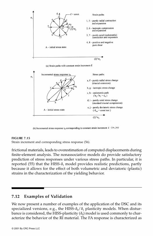
© 2001 By CRC Press LLC
frictional materials, leads to overestimation of computed displacements duringfinite-element analysis. The nonassociative models do provide satisfactoryprediction of stress responses under various stress paths. In particular, it isreported (55) that the HISS-�1 model provides realistic predictions, partlybecause it allows for the effect of both volumetric and deviatoric (plastic)strains in the characterization of the yielding behavior.
7.12 Examples of Validation
We now present a number of examples of the application of the DSC and itsspecialized versions, e.g., the HISS-�0/�1 plasticity models. When distur-bance is considered, the HISS-plasticity (�0) model is used commonly to char-acterize the behavior of the RI material. The FA response is characterized as
FIGURE 7.15Strain increment and corresponding stress response (56).

© 2001 By CRC Press LLC
constrained-liquid or constrained liquid-solid (critical state), Chapter 4. Onlya few validations are presented, while references are given for other materials.
The observed laboratory behavior of the materials considered is used tofind the parameters by employing the procedures described in this chapterand in Chapters 5 and 6. The values of parameters are given for most of theexamples.
The incremental equations, Eq. (7.44), are used to predict the responsesunder different factors such as stress path, type of loading, and initial condi-tions such as confining pressure and density. The incremental equations areintegrated for the initial loading such as hydrostatic. Based on the state ofstress at the end of the initial loading, the values of parameters such as thehardening function (�0) and the disturbance (D0) are computed. Then theequations are integrated for the subsequent shear loading under a givenstress path. The validations are often obtained for the test data used to findthe parameters, and for independent tests not used in finding the parameters;the latter provides a more rigorous validation.
In the case of frictional and geologic materials, the response is affected bymean pressure. Hence, tests are usually performed under different initialmean pressures or confining stresses. Also, compressive behavior is often sig-nificant; hence, tests are usually performed under compression loading, withthe assumption that compression is positive. Geologic materials involve ini-tial compressive stresses. Under loading, the compressive stresses mayincrease or decrease. The latter is often termed as an extension. To determinetensile behavior, sometimes direct tension or indirect (e.g., Brazilian split cyl-inder) tests are performed.
FIGURE 7.16Unit response envelopes for Leighton Buzzard sand with HISS-�1 mode. (From Ref. 55. Withpermission.)

© 2001 By CRC Press LLC
Example 7.4 Initial Conditions
Hardening:The expression of � can be obtained from Eq. (7.1) as
(4a)
The initial value �0 can be found by substituting in Eq. (4a), J1, J2D, and Sr
computed from the initial or in situ stresses, x , y , �xy , for two-dimensionaland x, y, z, �xy, �yz, �zx for three-dimensional problems. Now from Eq. (7.11a),
(4b)
Then, substitution of �0 in Eq. (4b) gives the value of the initial plastic straintrajectory, �0.
If the initial loading can be assumed to be proportional, the (initial) volu-metric plastic strain trajectory, �v0, can be found as (57)
(4c)
Then the initial deviatoric plastic strain trajectory, �D0, is evaluated from
(4d)
In the case of hydrostatic initial stress (x � y � z ; �xy � �yz � �zx � 0), forexample, in the triaxial test, Eq. (4a) simplifies to
(4e)
Disturbance. The initial disturbance, D0, can be found using, e.g., Eq.(3.15) or (3.16). Here it is necessary to have the knowledge of the initial (devi-atoric) plastic strain trajectory, which is often difficult to find. However, lab-oratory tests can be performed, say, on an initially anisotropic material and�orwith initial flaws (microcracks), under a small hydrostatic loading. Such aloading will cause shear strains in the specimens, which can be used to
� �J2D
J12 1 �Sr�( )m
-------------------------------------�
J1
pa----
2�n
�
� a1��0( )1��1�
�v0
�0�Q�ii----------
3�Q�
˜
-------- �Q�
˜
--------
1�2-----------------------------------�
�D0 �02
�v02
��
�0 �J1
pa----
2�n
�
�0 �v0 a1 �0�( )1��1� �
�D0 0�
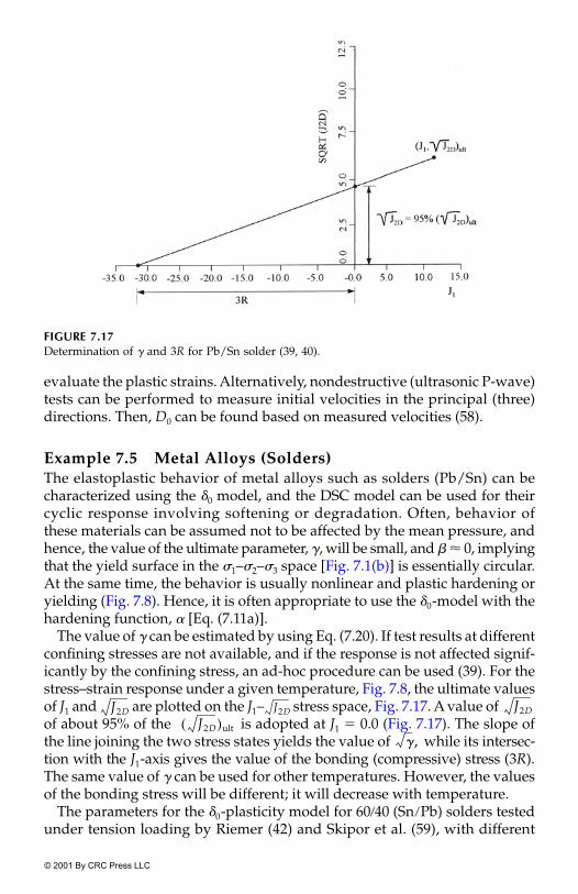
© 2001 By CRC Press LLC
evaluate the plastic strains. Alternatively, nondestructive (ultrasonic P-wave)tests can be performed to measure initial velocities in the principal (three)directions. Then, D0 can be found based on measured velocities (58).
Example 7.5 Metal Alloys (Solders)The elastoplastic behavior of metal alloys such as solders (Pb/Sn) can becharacterized using the �0 model, and the DSC model can be used for theircyclic response involving softening or degradation. Often, behavior ofthese materials can be assumed not to be affected by the mean pressure, andhence, the value of the ultimate parameter, �, will be small, and � � 0, implyingthat the yield surface in the 1–2–3 space [Fig. 7.1(b)] is essentially circular.At the same time, the behavior is usually nonlinear and plastic hardening oryielding (Fig. 7.8). Hence, it is often appropriate to use the �0-model with thehardening function, � [Eq. (7.11a)].
The value of � can be estimated by using Eq. (7.20). If test results at differentconfining stresses are not available, and if the response is not affected signif-icantly by the confining stress, an ad-hoc procedure can be used (39). For thestress–strain response under a given temperature, Fig. 7.8, the ultimate valuesof J1 and are plotted on the J1– stress space, Fig. 7.17. A value of of about 95% of the is adopted at J1 � 0.0 (Fig. 7.17). The slope ofthe line joining the two stress states yields the value of while its intersec-tion with the J1-axis gives the value of the bonding (compressive) stress (3R).The same value of � can be used for other temperatures. However, the valuesof the bonding stress will be different; it will decrease with temperature.
The parameters for the �0-plasticity model for 60�40 (Sn�Pb) solders testedunder tension loading by Riemer (42) and Skipor et al. (59), with different
FIGURE 7.17Determination of � and 3R for Pb/Sn solder (39, 40).
J2D J2D J2D
J2D( )ult
�,

© 2001 By CRC Press LLC
temperatures and strain rates, were computed by using the foregoing proce-dures; details are given elsewhere (39, 40). Tables 7.4(a) and 7.5(a) show typicalparameters for the solder at � 0.002�sec and 0.0002 �sec, respectively, andfor different temperatures. The parameters for the temperature dependence,Eq. (7.29), are shown in Tables 7.4(b) and 7.5(b), respectively. Details of theviscoplastic model are given in Chapter 8.
The disturbance parameters were found from the cyclic test data (Fig. 7.18)reported in (60). Their values are shown in Table 7.6. A number of other testdata for different solders (61–64) were also used to find parameters for differ-ent and similar solders.
Figure 7.19 (a)–(d) show typical comparisons between predicted and observedstress–strain data for different solders (64). Figure 7.19(a)–(c) show plastichardening results for 63/37 (Sn�Pb) solder at T � 373K, � 0.01�sec (59); for95�3 (Pb�Sn) solder, T � 100%C (61), and for 60�40 (Sn/Pb) solder, T � �50%Cand � 0.001�sec (63). The cyclic stress–strain response showing degrada-tion was predicted using the DSC with the �0-model for the RI behavior, for95�5 (Pb�Sn) solder at T � 20%C (62). It can be seen that the HISS-�0 and DSCmodels provide very good predictions for the plastic yielding and degrada-tion responses of Pb�Sn solders.
TABLE 7.4(a)
Parameters for Solder (Pb40/Sn60) at � 0.002/sec: �0-Model (39)
Temperature (K) 208 273 348 373
E (GPa) 26.1 24.1 22.45 22.00� 0.380 0.395 0.408 0.412
�T (1/K) � 2.75 2.93 3.11 3.16� 0.00083 0.00082 0.00082 0.00081� 0.0 0.0 0.0 0.0n 2.1 2.1 2.1 2.1
a1 (� ) 8.3 2.93 1.25 0.195�1 0.431 0.553 0.626 0.849
�1 (average)} 0.615y, yield stress (MPa) 37.241 31.724 20.690 15.172
Bonding stress, R (MPa) 395.80 288.20 175.20 122.10
TABLE 7.4(b)
Parameters for Temperature Dependence, Eq. (7.29) (39)
Parameter p300 c
E 23.45 (GPa) �0.292� 0.40 0.14�T 3 � (1�K) 0.24� 0.00082 �0.034� 0.05 � �5.5R 240.67 (MPa) �1.91
10 6�
10 6�
10 6�
10 4�

© 2001 By CRC Press LLC
7.12.1 Examples of Geologic Materials
Comprehensive laboratory triaxial tests on cylindrical specimens andmultiaxial tests on cubical specimens have been performed and wereavailable for a number of geologic materials such as sands, clays, androcks. These tests are performed at different initial confining pressuresand densities, and stress paths [Fig. 7.13(b)]. Only typical materials areconsidered here.
Parameters for the �0- and �1-HISS plasticity models were determinedusing the foregoing procedures. Table 7.7 shows the values of the parametersfor three dry sands: Ottawa, Leighton Buzzard, and Munich for the �0- and�1-models (3, 19, 20, 65, 66). Table 7.8(a) and (b) shows the �0- and disturbanceparameters for a saturated marine clay (32) and Leighton Buzzard sand (66),respectively, and Table 7.8(c) shows parameters for a saturated sand (67, 68).Table 7.9 shows parameters for three rocks (33, 34).
TABLE 7.5(a)
Material Parameters for 60/40 (Sn/Pb) Solder at Different Temperature for = 0.0002�sec: �0-Model (39)
Temperature (K) 208 273 298 348 373
E (GPa) 26.10 24.10 23.50 22.45 22.00� 0.380 0.395 0.400 0.408 0.412
�T (1/K) � 2.75 2.93 3.00 3.11 3.16� 0.00083 0.00082 0.00082 0.00081 0.00079� 0.0 0.0 0.0 0.0 0.0n 2.1 2.1 2.1 2.1 2.1
a1 (� ) 0.30 0.16 0.024 0.04 0.11�1 0.270 0.330 0.570 0.45 0.35
�1 (average) 3.94y, yield stress
(MPa)34.48 27.59 22.41 14.48 8.28
R (MPa) 433.80 284.58 217.47 116.57 73.90
TABLE 7.5(b)
Parameters for Temperature Dependence, Eq. (7.29) (39)
Parameter p300 c
E 23.45 (GPa) �0.292� 0.40 0.14�T 3.0 � (1�K) 0.24� 0.00082 �0.072� 0.35 � �2.60R 217.47 (MPa) �2.95
10 6�
10 4�
}
10 6�
10 4�
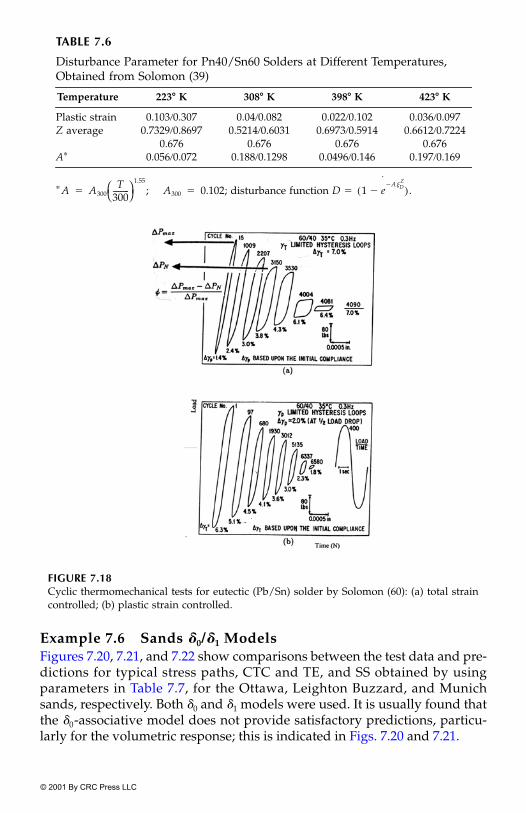
© 2001 By CRC Press LLC
Example 7.6 Sands �0/�1 ModelsFigures 7.20, 7.21, and 7.22 show comparisons between the test data and pre-dictions for typical stress paths, CTC and TE, and SS obtained by usingparameters in Table 7.7, for the Ottawa, Leighton Buzzard, and Munichsands, respectively. Both �0 and �1 models were used. It is usually found thatthe �0-associative model does not provide satisfactory predictions, particu-larly for the volumetric response; this is indicated in Figs. 7.20 and 7.21.
TABLE 7.6
Disturbance Parameter for Pn40/Sn60 Solders at Different Temperatures, Obtained from Solomon (39)
Temperature 223� K 308� K 398� K 423� K
Plastic strain 0.103�0.307 0.04�0.082 0.022�0.102 0.036�0.097Z average 0.7329�0.8697 0.5214�0.6031 0.6973�0.5914 0.6612�0.7224
0.676 0.676 0.676 0.676A� 0.056�0.072 0.188�0.1298 0.0496�0.146 0.197�0.169
� ; disturbance function D �
FIGURE 7.18Cyclic thermomechanical tests for eutectic (Pb/Sn) solder by Solomon (60): (a) total straincontrolled; (b) plastic strain controlled.
A A300T
300---------
1.55
;� A300 0.102� 1 eA�D
Z�
�( )˙
.

© 2001 By CRC Press LLC
TABLE 7.7
Parameters for Dry Sands
SandParameter Ottawa Leighton Buzzard Munich
E MPa 262 79 63(psi) (38,000) (11,500) (9,200)� 0.37 0.29 0.21� 0.124 0.102 0.105� 0.494 0.362 0.747N 3.0 2.5 3.20
0.135 0.1258
2.5 � 450 1355
�1 0.370 0.0047 .001
1.02 1.11R 0.00 0.00 0.00� 0.265 0.290 0.35
Eq. (7.11a)Eq. (7.11c)
FIGURE 7.19 Typical comparisons between model predictions and test data (39, 64): (a) 63�37 (Sn�Pb),T � 373 K, � 0.01�sec (59); (b) 95�3 (Pb�Sn), T � 100%C (61); (c) 60�40 (Sn�Pb), T � �50%C,
� 0.01�sec (63); (d) 95/5 (Pb�Sn), T � 20%C (62, 64).
h1��
a1�
10 3� h2��
h3��
h4��
�
��
o TEST DATAX SIMULATION
70
60
50
40
30
20
10
00 2 4 6 8
strain (%)
7
6
5
4
3
2
1
00 0.5 1 1.5 2 2.5 3 3.5 4
Strain (%)
BackpredictedLabo
Strain (%)
70
60
50
40
30
20
10
00 5 10 15 20
Savage and Cotton (1990) Backpredicted by DSC
Stress Strain (%)-1500
1000
-1000
500
-500
00 5-5 10-10 15-15 20-20 25-25
Laboratory Data Mir, et al.Backpredicted by DSC

© 2001 By CRC Press LLC
Example 7.7 Saturated Clay and Dry Sand: DSC ModelClay: Figures 7.23 and 7.24 show comparisons between DSC predictionsand observed laboratory undrained behavior of one-way cyclic (stress doesnot change sign) and two-way cyclic (stress changes sign) behavior for asaturated marine clay tested under both cylindrical triaxial and multiaxial
TABLE 7.8a
Parameters for Saturated Clay: DSC Model (32)
Parameter Value
E, MPa (psi) 10(1500)
� 0.35� 0.047� 0.00n 2.80
0.00010.78
0.0694� 0.169eoc 0.903A 1.73Z 0.309Du 0.75
�In Eq. (7.11b) with h3 � h4 � 0.
TABLE 7.8b
Parameters for Dry Leighton Buzzard Sand: DSC Model (66)
Parameter Value
E, MPa (psi) 118(17200)
� 0.30� 0.065� 0.65n 2.50 a0 0.00342a2 0.01841 in Eqs. (7.b) and (7.c)�0 0.3294�2 0.83
0.20� 0.13eoc 0.75A0 3.49A3 �3.34A4 3.28 in Eqs. (7.d), (7.e), and (7.f)Z0 0.580Z1 0.098
h1
h2 �
m
m

© 2001 By CRC Press LLC
conditions (32); the parameters are given in Table 7.8(a). Here, � initialeffective mean stress and e0 � void ratio. The stress–strain behavior in termsof (1 � 3) vs. 1, 2, and 3 (Fig. 7.23) is simulated very well by the DSCmodel, including degradation in the later stages. These figures also show thepredicted relatively intact (RI) behavior according to the �0-associative plas-ticity model.
The two-way cyclic behavior is also predicted very well by the DSC model,including the degradation with cycles of loading [Fig. 7.24(a)] and the stresspaths followed [Fig. 7.24(b)]. The predicted pore water pressure responsealso shows satisfactory correlation with the observations [Fig. 7.24(c)]. Thepore water pressure, p, was computed using the following equation:
(7a)
TABLE 7.8(c)
Parameters for Saturated Sand: �0-Model (67)
E, MPa 140(psi) (20,420) � 0.15� 0.636� 0.60n 3.0a1 0.16 �
�1 1.17R 0.00
TABLE 7.9
Parameters for Rocks (35, 36)
RockParameter Soap Stone Rock Salt Sandstone
E, MPa 9,150 21,000 25,500(psi) (1,328 � ) (3,050 � ) (3,700 � )
� 0.0792 0.27 0.11 � 0.0470 0.0945 0.0774
�0.750 0.990 0.767 0.0465 0.00048 0.0020
n 7.0 3.0 7.20a1 0.177 � 1.80 � 0.467 ��1 0.747 0.2322 0.345
R, MPa 1.067 1.80 2.90(psi) (155) (260) (420)
� — 0.275 —
*Eq. (7.15a)**Eq. (7.15b)
10 4�
103 103 103
�0
�1 � �
�1 ��
10 2� 10 5� 10 2�
�0
pJ1t J1
a�
3------------------�

© 2001 By CRC Press LLC
where J1t is the first invariant of the total stress tensor, and is the firstinvariant of the average (predicted) effective stress.
Dry Sand: The Leighton Buzzard (LB) sand was tested using the cylindricaltriaxial device (66). The DSC model, Chapter 4, with the �0-model for the RIbehavior was used to characterize the behavior of the sand, which exhibitedsoftening response for higher densities (Dr) and lower mean pressures (0 � p0).The parameters for the sand are shown in Table 7.8(b). Here, the hardeningand disturbance parameters were expressed as dependent on relative density,Dr , and �or initial confining stress, 0:
(7b)
(7c)
(7d)
FIGURE 7.20Comparisons between model predictions and test data for Ottawa sand: �0 � 1.73 g/cc;1 psi � 6.89 kPa (20).
J1a
a1 a0ln Dr ln a2��
�1 �0 �2Dr��
A A0 A2Dr��

© 2001 By CRC Press LLC
(7e)
(7f)
Figure 7.25 shows comparisons between the DSC predictions and testdata for Dr � 95% and 0 � 276 kPa (40 psi) under the CTC stress path. Thefigure also shows predictions according to the �0-model used to simulatethe RI behavior. It can be seen in Fig. 7.25(b) that the �0-associative model
FIGURE 7.21Comparisons between model predictions and test data for Leighton Buzzard sand: SS (0 � 20psi), �0 � 1.74 g/cc, 1 psi � 6.89 kPa (4, 19, 66).
A2 A3 A40
pa-----
��
Z Z0 Z10
pa-----
��

© 2001 By CRC Press LLC
(RI) predicts a much higher volume change compared to the test data. How-ever, the use of the DSC model provides much improved predictions. Thus,the constraining effect due to friction is included in the DSC model, and itmay not be necessary to use a nonassociative model.
Example 7.8 Saturated Sand (67): �0-ModelTable 7.8(c) shows the parameters from test on sand C reported by Castro(68). The sand is a natural beach sand from deposits at Huachipato, Chile,and it is uniform fine sand with specific gravity, Gs � 2.87 and uniformitycoefficient � 2.3.
Figure 7.26 shows comparisons between prediction (�0-plasticity model)and test data for the undrained behavior of sand under CTC path with 0 �98 kPa (14.21 psi). Both the stress–strain and pore water pressure responsesare predicted well by the plasticity model.
FIGURE 7.22Comparisons between model predictions and test data for Munich sand: nonassociative �1-model: SS (0 � 13 psi), �0 � 2.03 g/cc; 1 psi � 6.89 kPa (20).

© 2001 By CRC Press LLC
Example 7.9 RocksLaboratory stress–strain behavior of a soap stone and a rock salt, Table 7.9,were obtained from tests with cubical specimens (33, 34, 36). The test datausing cubical specimens for a sandstone found in Japan, reported by Nishidaet al. (69), were used.
Figures 7.27 to 7.29 show comparisons between predictions using the �0-model for the soap stone, rock salt, and sandstone; both the �0- and �1-modelswere used for the rock salt. The results for the soap stone and sandstone areunder the SS and TC paths, while those for the rock salt are for the CTC path.It can be seen that the volumetric strains are predicted better for the rock saltby the �1-model (Fig. 7.28), while the �0-model shows discrepancies in thevolumetric response for the other two rocks, Figs. 7.27 and 7.29; use of the �1-model would improve the predictions.
FIGURE 7.23Comparisons between model predictions and one-way cyclic test data for marine clay: CTC( � 110 psi); e0 � 0796 (32), 1 psi � 6.89 kPa.�0
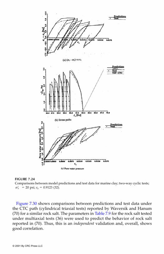
© 2001 By CRC Press LLC
Figure 7.30 shows comparisons between predictions and test data underthe CTC path (cylindrical triaxial tests) reported by Waversik and Hanum(70) for a similar rock salt. The parameters in Table 7.9 for the rock salt testedunder multiaxial tests (36) were used to predict the behavior of rock saltreported in (70). Thus, this is an independent validation and, overall, showsgood correlation.
FIGURE 7.24Comparisons between model predictions and test data for marine clay; two-way cyclic tests;
� 20 psi; e0 � 0.9123 (32).�0

© 2001 By CRC Press LLC
Example 7.10 Concrete: �0-Plasticity ModelTable 7.10 shows material parameters for the �0-model for a plain concretetested under stress-controlled multiaxial loading. Cubical specimens weretested under different initial confining pressures and stress paths [Fig. 7.13(b)](35). Figure 7.31(a) shows comparisons between predictions and test data(solid circles and triangles) for the ultimate behavior under different stresspaths and in different stress spaces. Figure 7.31(b) shows a typical comparisonbetween predictions of stress–strain and volumetric responses and test datafor the SS stress path with 0 � 31 MPa (4.5 � psi) and the TE stress pathwith 0 � 28 MPa (4.0 � psi).
The parameters (Table 7.10) were determined from test data under variousstraight-line stress paths [Fig. 7.13(b)]. An independent test was performed in
FIGURE 7.25Comparisons between model (DSC) predictions and test data for Leighton Buzzard sand(CTC, 0 � 40 psi); Dr � 95% (66).
103
103

© 2001 By CRC Press LLC
FIGURE 7.26Comparisons between model predictions and test data for saturated sand: CTC (0 � 14.21psi); 1 psi � 6.89 kPa (67).
FIGURE 7.27Comparisons between model predictions and test data for soap stone. (From Ref. 33. Re-printed with permission from Elsevier Science.)

© 2001 By CRC Press LLC
which the stress path followed was circular [Fig. 7.13(b)]. This test involved�oct � 7.0 kPa and 0 � 28.0 kPa. Figure 7.32 shows comparisons betweenpredicted and observed strains under the circular stress path [Fig. 7.13(b)].This is an independent validation and shows satisfactory predictions by the�0-model.
Example 7.11 Concrete: DSC ModelStrain-controlled tests on cubical specimens of plain concrete were reportedby Van Mier (71). The parameters for the DSC model were obtained using thetests under uniaxial and proportional loading stress paths (72, 73); they areshown in Table 7.10. In the DSC model, the RI behavior was simulated by
FIGURE 7.28Comparisons between model predictions and test data for rock salt: CTC (0 � 0.0 MPa).(From Ref. 36, ©American Geophysical Union. Reprinted with permission.)

© 2001 By CRC Press LLC
using the �0-plasticity model, and for the FA behavior it was assumed thatmaterial in that state can carry hydrostatic stress but no shear stress.
Figure 7.33 shows comparisons between predicted and observed testresults in terms of �oct vs. 1, �oct vs. 2, and v vs. 1 responses for the loadingpath 1�2 � 1�3 � 10 (71).
Example 7.12 Geologic (Unbound) Materials in Pavements: Repeated LoadingBonaquist (74) and Bonaquist and Witczak (75) conducted a comprehensiveseries of laboratory triaxial tests on geologic materials (base, subbase, sub-grade) in pavement structures. They used a simplified form of the HISS�0-model, without the term Fs in Eq. (7.1), to characterize the elastoplasticbehavior of the materials. They also developed procedures for reducing theparameters (e.g., by expressing some in terms of others) toward practicalapplication, and considered important factors such as pore water pressureeffects, partial saturation, and repeated loading permanent deformations
FIGURE 7.29.Comparisons between model predictions and test data for sandstone: TC (0 � 28.45 psi)(34); 1 psi � 6.89 kPa (35).

© 2001 By CRC Press LLC
leading to rutting in pavements. Table 7.11 shows the parameters for the threematerials. Determination of parameters involved numerical optimization inwhich the values of n and �1 were maintained at their average values of 3.25and 0.50, respectively. The hardening parameter, a1, was expressed in terms
FIGURE 7.30Comparisons between model predictions and test data for similar rock salt: CTC (0 � 3.45MPa). (From Ref. 36. ©American Geophysical Union. Reprinted with permission.)
15
10
5
0
-6 -4 -2 0 2 4
Associative
Nonassociative
Experimental
Strain Ez Ej . : Strain El . :
4
2
0
-2
0 1 2 3 4 5
Strain E1, %
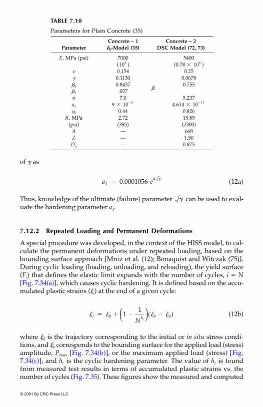
© 2001 By CRC Press LLC
of � as
(12a)
Thus, knowledge of the ultimate (failure) parameter can be used to eval-uate the hardening parameter a1.
7.12.2 Repeated Loading and Permanent Deformations
A special procedure was developed, in the context of the HISS model, to cal-culate the permanent deformations under repeated loading, based on thebounding surface approach [Mroz et al. (12); Bonaquist and Witczak (75)].During cyclic loading (loading, unloading, and reloading), the yield surface(Fi) that defines the elastic limit expands with the number of cycles, i � N[Fig. 7.34(a)], which causes cyclic hardening. It is defined based on the accu-mulated plastic strains (�i) at the end of a given cycle:
(12b)
where �0 is the trajectory corresponding to the initial or in situ stress condi-tions, and �b corresponds to the bounding surface for the applied load (stress)amplitude, Pmax [Fig. 7.34(b)], or the maximum applied load (stress) [Fig.7.34(c)], and hc is the cyclic hardening parameter. The value of hc is foundfrom measured test results in terms of accumulated plastic strains vs. thenumber of cycles (Fig. 7.35). These figures show the measured and computed
TABLE 7.10
Parameters for Plain Concrete (35)
ParameterConcrete – 1 �0-Model (35)
Concrete – 2 DSC Model (72, 73)
E, MPa (psi) 7000 5400( ) (0.78 � )
� 0.154 0.25� 0.1130 0.0678�0 0.8437
�0.755
�1 .027n 7.0 5.237a1 9 � 4.614 ��1 0.44 0.826
R, MPa 2.72 15.85(psi) (395) (2300)
A — 668Z — 1.50Du — 0.875
106 106
10 3� 10 11�
a1 0.0001056 e4 ��
�
�i �0 11
Nhc--------�
�b � �0( )��

© 2001 By CRC Press LLC
plastic strains for subgrade and base materials, respectively. Figure 7.36shows comparisons between predictions and measurements for a multipleload-level test (74). Here, during a load-level, the given stress wascycled for a fixed number of cycles; each level involved different values of J1
and .
Example 7.13 Rock (Granite) under High PressureTriaxial compression tests were performed by Alheid (76) on granite speci-mens under confining pressures up to 4.5 kb (450 MPa) and temperature upto 350%C. Figure 7.37 shows laboratory test behavior of the granite in terms ofstress difference (1 � 3) vs. 1 and (1 � 3) vs. v (� 1 � 2 � 3). Thebehavior exhibits strain softening. However, the �0-plasticity model was used
FIGURE 7.31Comparison between model predictions and test data for plain concrete (35).
J1, J2D( )
J2D

© 2001 By CRC Press LLC
FIGURE 7.31(continued)
FIGURE 7.32Comparisons between model predictions and test data for plain concrete: circular stresspath, 0 � 4 ksi, �oct � 1 ksi; 1 psi � 6.89 kPa (35).

© 2001 By CRC Press LLC
FIGURE 7.33Comparisons between model predictions and test data for plain concrete: loading path,1/2 � 2/3 � 10.0. (From Ref. 72, with permission from Elsevier Science.)
TABLE 7.11
Parameters for Pavement Materials (74)
Material
ParameterBase:
Crushed AggregateSubbase:
Silty SandSubgrade:Silty Sand
� 0.265 0.0756 0.0328a1 8.31 � 2.93 � 2.45 ��1 0.50 0.50 0.50n 3.25 3.25 3.25
R (kPa) 0.00 14.00 31.00
10 4� 10 4� 10 4�

© 2001 By CRC Press LLC
to characterize the elastoplastic hardening behavior (77). The parameters forthe �0-model are given in Table 7.12.
Test data on a similar granite reported by Mogi (78) using a multiaxialdevice under compression and extension paths were used to find the value of� using Eq. (7.13d), with tan �C � 0.418 and tan �E � 0.258. The value of R wasadopted equal to about 10% of the uniaxial compressive strength for thegranite of about 180 MPa.
Typical comparisons for the (1 � 3) vs. 1 responses for 0 � 78 and 157 MPaare shown in Fig. 7.38(a) and (b), respectively. It can be seen that the �0-modelpredicts the elastoplastic behavior very well. It is reported (76) that the rock expe-riences microcracking and slip, resulting in degradation and strain softening(Fig. 7.37). Hence, to characterize the complete response, it would be appropriateto use the DSC model.
Example 7.14 Optimum Tests and Sensitivity of ParametersTo determine material parameters, it is desirable to use laboratory tests underas many stress paths and (initial) conditions as possible. Then the constitutivemodel calibrated on the basis of the tests would include effects of the stress
FIGURE 7.34Cyclic hardening under repeated loading.

© 2001 By CRC Press LLC
paths and conditions that influence the field behavior. However, in practice,it may not be possible to perform many such tests, and it may become neces-sary to estimate the parameters based on the optimum (or minimum) num-ber of available tests.
In order to determine the optimum number of tests, detailed parametricevaluations were performed. Here, predictions for stress–strain–volumechange behavior of a sand (79) tested using the standard and commonlyavailable triaxial device with cylindrical specimens were compared usingparameters determined from various sets of tests under different stress paths.
The parameter � was expressed as function of J1 as in Eq. (7.15b). The non-associative parameter � was assumed to be a function of the stress ratio, Sr
[Eq. (7.1)] as
(13a)
FIGURE 7.35(A)Comparisons between model (�0-cyclic hardening) predictions and test data for accumulatedplastic strains: subgrade (74).
� �1 �2Sr��
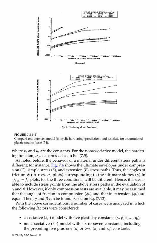
© 2001 By CRC Press LLC
where �1 and �2 are the constants. For the nonassociative model, the harden-ing function, �Q, is expressed as in Eq. (7.5).
As noted before, the behavior of a material under different stress paths isdifferent; for instance, Fig. 7.4 shows the ultimate envelopes under compres-sion (C), simple stress (S), and extension (E) stress paths. Thus, the angles offriction � (in � vs. n plots) corresponding to the ultimate slopes (�) in
plots, for the three conditions, will be different. Hence, it is desir-able to include stress points from the above stress paths in the evaluation of� and �. However, if only compression tests are available, it may be assumedthat the angle of friction in compression (�C) and that in extension (�E) areequal. Then, � and � can be found based on Eq. (7.13).
With the above considerations, a number of cases were analyzed in whichthe following factors were considered:
• associative (�0-) model with five plasticity constants (�, �, n, a1, �1);• nonassociative (�1-) model with six or seven constants, including
the preceding five plus one (�) or two (�1 and �2) constants;
FIGURE 7.35(B)Comparisons between model (�0-cyclic hardening) predictions and test data for accumulatedplastic strains: base (74).
J2D J1�

© 2001 By CRC Press LLC
• straight and curved ultimate envelope with one (�) or two (� and�1) constants [Eq. (7.15b)];
• constants found as average values from nine tests for ultimateenvelopes, five shear tests under different stress paths (CTC, TC,and TE) or two tests (one CTC and one TE) or only one test (CTC)with the assumption of �C � �E.
FIGURE 7.36Comparisons between model (�0-cyclic hardening ) predictions and test data for accumulatedplastic strains: multiple-load permanent deformation test (74).
FIGURE 7.37Triaxial test data for granite at different initial confining pressures, 0 � 3 (76, 77).

© 2001 By CRC Press LLC
TABLE 7.12
Parameters for Granite (77)(With Permission)
Parameter Value
E 6.67 � MPa� 0.26� 0.038� 0.75N 8.30a1 9.8 �
�1 0.72R 18 MPa
FIGURE 7.38Comparisons between model (�0) predictions and test data for granite (77).
104
10 30�
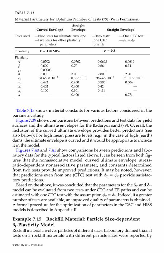
© 2001 By CRC Press LLC
Table 7.13 shows material constants for various factors considered in theparametric study.
Figure 7.39 shows comparisons between predictions and test data for yieldsurfaces and the ultimate envelopes for the Badarpur sand (79). Overall, theinclusion of the curved ultimate envelope provides better predictions (seealso below). For high mean pressure levels, e.g., in the case of high (earth)dams, the ultimate envelope is curved and it would be appropriate to includeit in the model.
Figures 7.40 and 7.41 show comparisons between predictions and labo-ratory data for the typical factors listed above. It can be seen from both fig-ures that the nonassociative model, curved ultimate envelope, stress-ratio-dependent nonassociative parameter, and constants determinedfrom two tests provide improved predictions. It may be noted, however,that predictions even from one (CTC) test with �C � �E provide satisfac-tory predictions.
Based on the above, it was concluded that the parameters for the �0- and �1-model can be evaluated from two tests under CTC and TE paths and can beestimated with one CTC test with the assumption �C � �E. Indeed, if a greaternumber of tests are available, an improved quality of parameters is obtained. A formal procedure for the optimization of parameters in the DSC and HISSmodels is described in Appendix II.
Example 7.15 Rockfill Material: Particle Size-dependent �1-Plasticity ModelRockfill material involves particles of different sizes. Laboratory drained triaxialtests on a rockfill materials with different particle sizes were reported by
TABLE 7.13
Material Parameters for Optimum Number of Tests (79) (With Permission)
Curved EnvelopeStraight
Envelope Straight Envelope
Tests used —Nine tests for ultimate envelope—Five tests for other plasticity
parameters
—Two tests: one CTC one TE
— One CTC test—�C � �E
Elasticity E � 150 MPa � 0.3
Plasticity� 0.0702 0.0702 0.0698 0.0619� �0.690 0.70 0.66 0.74�1 0.00003 — — —n 3.00 3.00 2.80 2.90a1 31.66 � 38.5 � 36.64 � 31.31 ��1 0.493 0.450 0.505 0.504�1 0.402 0.400 0.42 —�2 0.100 0.101 0.111 —� — 0.400 — 0.271
�
10 4� 10 4� 10 4� 10 4�
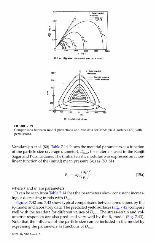
© 2001 By CRC Press LLC
Varadarajan et al. (80). Table 7.14 shows the material parameters as a functionof the particle size (average diameter), Dmax, for materials used in the RanjitSagar and Purulia dams. The (initial) elastic modulus was expressed as a non-linear function of the (initial) mean pressure (0) as (80, 81)
(15a)
where k and n� are parameters.It can be seen from Table 7.14 that the parameters show consistent increas-
ing or decreasing trends with Dmax.Figures 7.42 and 7.43 show typical comparisons between predictions by the
�1-model and laboratory data. The predicted yield surfaces (Fig. 7.42) comparewell with the test data for different values of Dmax. The stress–strain and vol-umetric responses are also predicted very well by the �1-model (Fig. 7.43).Note that the influence of the particle size can be included in the model byexpressing the parameters as functions of Dmax.
FIGURE 7.39Comparisons between model predictions and test data for sand: yield surfaces (79)(withpermission).
Ei kpa0
pa-----
n�
�

© 2001 By CRC Press LLC
Example 7.16 Silicon Crystal with Dislocation: Disturbance ModelDillon et al. (82) proposed a three-dimensional generalization of the constitu-tive model by Haasen (83) for the characterization of thermomechanicalbehavior of silicon crystals (ribbons) with dislocations. Figure 7.44 showsstress–strain behavior (predicted by their model); it is affected by factors suchas (initial) dislocation density (N0), temperature (T ), strain rate , andimpurities such as oxygen and nitrogen.
The DSC model was used to characterize the behavior of the silicon crys-tals, and a correlation was established between disturbance and dislocation(see Eq. 3.25a, Chapter 3) (84). In the DSC, the RI behavior was simulated byusing a linear elastic model (Chapter 5) in which the elastic moduli wereexpressed as (82)
(16a)
(16b)
FIGURE 7.40Comparisons between model predictions and test data: parametric sensitivity analyses, TC(0 � 137.3 kPa) (79)(with permission).
( )
E 1.7 1011 2.771 104 T( )2pa����
G 6.81E�17pa�

© 2001 By CRC Press LLC
It can also be simulated using the �0-plasticity model. The disturbance func-tion, Eq. (3.16b), was used and its values from the stress–strain data (Fig. 7.44)were evaluated based on the following equation (Eq. 3.7):
(16c)
The parameters in Eq. (3.16b), h, and s, were found using the proceduredescribed in Chapter 3 (Fig. 3.18). The parameters and s were found to berelatively constant under T, N0, and and their average values were foundto be 1.354 and 1.20, respectively. The parameter h was found to be dependenton T and N0 and was expressed as
(16d)
FIGURE 7.41Comparisons between model predictions and test data: parametric sensitivity analyses, CTC(0 � 274.6 kPa) (79) (with permission).
D
i
a�
i
c
�------------------�
w,w
,
h N0, T( ) h300 N0( ) T300---------
n N0( )
�

© 2001 B
y CR
C P
ress LLC
TABLE 7.14
Rockfill Materials Parameters (80) (with permission)
Material Constants
Ranjit Sagar Dam Material Dmax (mm)
Purulia Dam MaterialDmax (mm)
10 25 50 80 25 50 80
Elasticityk 156.03 193.69 220.34 253.63 167.07 286.02 451.13n� 0.5768 0.6386 0.6683 0.7146 0.8162 0.6550 0.4068� 0.36 0.31 0.30 0.29 0.34 0.33 0.31
Ultimate� 0.0577 0.0630 0.0781 0.0811 0.0619 0.0617 0.0615� 0.71 0.72 0.73 0.74 0.72 0.72 0.72
Phase change, n 3 3 3 3 3 3 3Hardening
a1 0.158E-3 0.722E-4 0.605E-4 0.985E-5 0.310E-4 0.850E-4 0.130E-3�1 0.355 0.453 0.476 0.762 0.600 0.440 0.380
Nonassociative, � 0.20 0.25 0.22 0.22 0.23 0.20 0.17
© 2001 B
y CR
C P
ress LLC

© 2001 By CRC Press LLC
where h300 is the value of h at T � 300 K and is the exponent; both are depen-dent on N0 and were expressed as
(16e)
(16f)
FIGURE 7.42Comparisons between predictions and test data for yield surface for typical values of Dmax
(80) (with permission).
FIGURE 7.43Comparisons between predictions and test data for stress–strain and volume change responses(80) (with permission).
n
h300 N0( ) 1.195 3.675 10�9� N0��
n N0( ) 6.735� 2.577 10�9� N0��

© 2001 By CRC Press LLC
Hence, the disturbance function was expressed as
(16g)
The DSC equations [Eq. (3.1)] were integrated to predict the laboratorybehavior under different temperatures, strain rates, and dislocation densities(84). Typical results are presented in Figure 7.45(a) and (b), which show typicalcomparisons between predictions and test data for two conditions: (a) T �960%C, � 1.2 � and N0 � 2 � and (b) T � 1100%C, �4.8 � and N0 � 1.8 � The correlation is considered tobe highly satisfactory.
Application of the DSC model for the softening and stiffening responseof silicon with high levels of N0 and oxygen impurities is presented inChapter 10.
FIGURE 7.44Stress–strain data for silicon ribbon (82): (a) temperature, (b) strain rate, (c) initial dislocationdensity.
D Du 1.0 1.0�D
h N0, T( )----------------------�
1.254
�
�1.2
�
10�4 s�1, 104 cm�2 10�4 s�1, 105 cm�2.

© 2001 By CRC Press LLC
References
1. Desai, C.S., “A General Basis for Yield, Failure and Potential Functions inPlasticity,” Int. J. Numer. Analy. Methods Geomech., 4, 1980, 361–375.
2. Desai, C.S. and Faruque, M.O., “Constitutive Model for Geologic Materials,”J. Eng. Mech., ASCE, 110, 9, 1984, 1391–1408.
3. Desai, C.S., Somasundaram, S., and Frantziskonis, G., “A Hierarchical Ap-proach for Constitutive Modelling of Geologic Materials,” Int. J. Numer. Anal.Methods in Geomech., 10, 3, 1986, 225–257.
4. Desai, C.S. and Wathugala, G.N., “Hierarchical and Unified Models for Solidsand Discontinuities,” Notes for Short Course, Tucson, Arizona, USA, 1987.
5. Desai, C.S., “Hierarchical Single Surface and the Disturbed State ConstitutiveModels with Emphasis on Geotechnical Applications,” Chapter 5 in Geotechni-cal Engineering, K.R. Saxena (editor), Oxford & IBH Publ. Co., New Delhi, India,1994.
FIGURE 7.45Comparisons between given and predicted curves for silicon ribbon for independent tests:(a) T � 960%C, � 1.2 � N0 � 2 � (b) T � 1100%C, � 4.8 �N0 � 1.8 � (84) (with permission).
50.0
40.0
30.0
20.0
10.0
0.00.0 0.001 0.002 0.0030.0005 0.0015 0.0025
(a)
Computed by Dillon et.al.Backpredicted by DSC
50.0
40.0
30.0
20.0
10.0
0.00.0 0.004 0.008 0.0120.002 0.006 0.010
(b)
Computed by Dillon et.al.Backpredicted by DSC
10�4 s�1, 104 cm�2, 10�4 s�1,105 cm�2
© 2001 By CRC Press LLC
6. Desai, C.S., “Constitutive Modelling Using the Disturbed State as Microstruc-ture Self-Adjustment Concept,” Chapter 8 in Continuum Models for Materialswith Microstructure, H.B. Mühlhaus (editor), John Wiley, U.K, 1995.
7. Matsuoka, H. and Nakai, T., “Stress-Deformation and Strength Characteristicsof Soil Under Three Different Principal Stresses,” Proc. Jap. Soc. Civil Engrs.,No. 232, 1974, 59–70.
8. Lade, P.V. and Duncan, J.H., “Elastoplastic Stress-Strain Theory for Cohesion-less Soil,” J. Geotech. Eng., ASCE, 101, 10, 1975, 1037–1053.
9. Lade, P.V. and Kim, M.K., “Single Hardening Constitutive Model for FrictionalMaterials. III. Comparisons with Experimental Data,” Computers and Geotech-nics, 6, 1988, 31–47.
10. Vermeer, P.A., “A Five-Constant Model Unifying Well-Established Concepts,”Proc. Int. Workshop on Constitutive Relations for Soils, Grenoble, 1982, 1984,175–197.
11. Mroz, Z., “On the Description of Anisotropic Work Hardening,” J. Mech. Phys.Solids, 15, 1967, 163–175.
12. Mroz, Z., Norris, V.A., and Zienkiewicz, O.C., “An Anisotropic HardeningModel for Soils and Its Application to Cyclic Loading,” Int. J. Numer. Analy.Methods Geomech., 2, 1978, 203–221.
13. Mroz, Z., Norris, V.A., and Zienkiewicz, O.C., “Application of an AnisotropicHardening Model in the Analysis of Elasto-plastic Deformation of Soils,” Geo-technique, 29, 1, 1979, 1–34.
14. Krieg, R.D., “A Practical Two-Surface Plasticity Theory,” J. Appl. Mech., 42, 1975,641–646.
15. Prevost, J.H., “Plasticity Theory of Soil Stress–Strain Behavior,” J. Eng. Mech.,ASCE, 104, 5, 1978, 1177–1194.
16. Dafalias, Y.F. and Popov, E. P., “A Model for Nonlinearly Hardening Materialsfor Complex Loading,” Acta Mech., 21, 3, 1975, 173–192.
17. Dafalias, Y.F., “A Bounding Surface Plasticity Model,” Proc. 7th Can. Cong. Appl.Mech., Sherbrooke, Canada, 1979.
18. Baker, R. and Desai, C.S., “Consequences of Deviatoric Normality in Plasticitywith Isotropic Hardening,” Int. J. Num. Analyt. Meth. Geomech., 6, 3, 1982,383–390.
19. Desai, C.S. and Hashmi, Q.S.E., “Analysis, Evaluation and Implementation ofa Nonassociative Model for Geologic Materials,” Int. J. Plasticity, 5, 1989,397–420.
20. Frantziskonis, G., Desai, C.S., and Somasundaram, S., “Constitutive Model forNonassociative Behavior,” J. of Eng. Mech., ASCE, 112, 1986, 932–946.
21. Desai, C.S., Letter to the Editor for “Single Surface Yield and Potential FunctionPlasticity,” by Lade, P.V. and Kim. M.K., Computers and Geotechnics, 7, 1989,319–335.
22. Desai, C.S., Discussion to “Single Hardening Model with Application to NCClay,” J. Geotech. Eng., ASCE, 118, 2, 1990, 337–340.
23. Roscoe, K.H., Schofield, A.N., and Wroth, C.P., “On Yielding of Soils,” Geotech-nique, 8, 1958, 22–53.
24. Schreyer, H.L., “A Third Invariant Plasticity Theory for Frictional Materials,”J. of Structural Mech., June 1983.
25. Sture, S., “Model by Prevost,” Proc., Workshop Session, Symposium on Implemen-tation of Computer Procedures and Stress–Strain Laws in Geotech. Eng., Chicago,IL, 1981.

© 2001 By CRC Press LLC
26. Somasundaram, S. and Desai, C.S., “Modelling and Testing for AnisotropicBehavior of Soils,” J. Eng. Mech., ASCE, 114, 1988, 1473–1496.
27. Desai, C.S. and Galagoda, H.M., “Earthquake Analysis with Generalized Plas-ticity Model for Saturated Soils,” J. Earthquake Eng. and Struct. Dyn., 18, 6, 1989,903–919.
28. Wathugala, G.W. and Desai, C.S., “Constitutive Model for Cyclic Behavior ofCohesive Soils, I: Theory,” J. Geotech. Eng., ASCE, 119, 4, 714–729.
29. Desai, C.S. and Zhang, D., “Viscoplastic Model with Generalized Yield Func-tion,” Int. J. Numer. Methods Geomech., 11, 1987, 603–620.
30. Desai, C.S., Samtani, N.C., and Vulliet, L., “Constitutive Modeling and Analysisof Creeping Slopes,” J. Geotech. Eng., ASCE, 121, 1, 1995, 43–56.
31. Samtani, N.C., Desai, C.S., and Vulliet, L., “An Interface Model to DescribeViscoplastic Behavior,” Int. J. Numer. Analyt. Methods Geomech., 20, 4, 1996,231–252.
32. Katti, D.R. and Desai, C.S., “Modelling and Testing of Cohesive Soil Using theDisturbed State Concept,” J. Eng. Mech., ASCE, 121, 1994, 648–658.
33. Desai, C.S. and Salami, M.R., “A Constitutive Model and Associated Testingfor Soft Rock,” Int. J. Rock Mech. & Min. Sc., 24, 5, 1987, 299–307.
34. Desai, C.S. and Salami, M.R., “A Constitutive Model for Rocks,” J. Geotech.Eng., ASCE, 113, 5, 1987, 407–423.
35. Salami, M.R. and Desai, C.S., “Constitutive Modelling of Concrete and RocksUnder Multiaxial Compressive Loading,” Report, Dept. of Civil Eng. and Eng.Mechs., University of Arizona, Tucson, AZ, 1986
36. Desai, C.S. and Varadarajan, A., “A Constitutive Model for Quasistatic Behaviorof Rock Salt,” J. of Geophys. Research, 92, B11, 1987, 11, 445–11, 456.
37. Lade, P.V., “Three-Parameter Failure Criterion for Concrete,” Proc. ASCE, 108,5, 1982, 850–863.
38. Hoek, E. and Brown, E.T., “Empirical Strength Criterion for Rock Masses,” J.Geotech. Eng., ASCE, 106, 9, 1980, 1013–1035.
39. Chia, J. and Desai, C.S., “Constitutive Modelling of Thermomechanical Re-sponse of Materials in Semiconductor Devices Using the Disturbed State Con-cept,” Report to NSF, Dept. of Civil Eng. and Eng. Mechs., University of Arizona,Tucson, AZ, 1994.
40. Desai, C.S., Chia, J., Kundu, T., and Prince, J.L., “Thermomechanical Responseof Materials and Interfaces in Electronic Packaging, Parts I & II,” J. of Elect.Packaging, ASME, 119, 1997, 294–300; 301–309.
41. Wathugala, G.W. and Desai, C.S., “Finite Element Dynamic Analysis of Non-linear Porous Media with Application to Piles in Saturated Clays,” Report toNSF, Dept. of Civil Eng. and Eng. Mechs., University of Arizona, Tucson, AZ,1990.
42. Riemer, D.C., “Prediction of Temperature Cycling Life for SMT SolderJoints on TCE-Mismatched Substrates,” Proc. Elect. Comp., IEEE, New Jer-sey, 1990, 418–423.
43. Desai, C.S. and Siriwardane, H.J., Constitutive Laws for Engineering Materials,Prentice-Hall, Englewood Cliffs, NJ, 1984.
44. Hill, R., The Mathematical Theory of Plasticity, Oxford Univ. Press, London.45. Drucker, D.C., “Some Implications of Work Hardening and Ideal Plasticity,”
Quart. Appl. Math., 7, 4, 1950, 411–418.46. Desai, C.S. and Abel, J.F., Introduction to the Finite Element Method, Van Nostrand
Reinhold Co., New York, 1972.

© 2001 By CRC Press LLC
47. Desai, C.S. and Kundu, T., Introductory Finite Element Method, CRC Press, BocaRaton, FL, 2000, under publication.
48. Faruque, M. and Desai, C.S., “Implementation of a General Constitutive Modelfor Geologic Materials,” Int. J. Numer. Analyt. Methods Geomech., 9, 5, 1985.
49. Potts, D.M. and Gens, A., “A Critical Assessment of Methods of Correctionsfor Drift from Time-Yield Surface in Elastoplastic Finite Element Analysis,” Int.J. Numer. Analy. Methods Geomech., 9, 1985, 149–159.
50. Sloan, S.W., “Substepping Schemes for the Numerical Integration of Elastoplas-tic Stress–Strain Relations,” Int. J. Num. Meth. in Eng., 24, 1987, 893–911.
51. Prager, W., “Non-isothermal Plastic Deformation,” Bol. Koninke, Nederl. Acad.Wet, 8(61/3), 1958, 176–182.
52. Ziegler, H., “A Modification of Prager’s Hardening Rule,” Quart. Appl. Math.,17, 1959, 55–65.
53. Chen, J. and Desai, C.S., “Optimization of the Disturbed State Concept for Con-stitutive Modelling, and Application in Finite Element Analysis, Report to NSF,Dept. of Civil Engng. and Engng. Mechanics, University of Arizona, Tucson,Arizona, 1997.
54. Gudehus, G., “Requirements for Constitutive Relations for Soils,” Chapter 4 inMechanics of Geomaterials, Z. Bazant (Editor), John Wiley & Sons, U.K., 1985,47–63.
55. Dolezalova, M., “Stress Path Analysis of Geotechnical Structures and Selectionof Constitutive Models for Geomaterials,” Proc. 9th Int. Conf. on Computer Methodsand Advances in Geomech., J.X. Yuan (Editor), A.A. Balkema, The Netherlands,1997, 123–132.
56. Dolezalova, M., Boudik, Z., and Hladik, I., “Numerical Testing and Comparisonof Constitutive Models of Geomaterials,” Acta Montana (Prague), Series A:Geodynamics, 1, 87, 1992, 33–56.
57. Desai, C.S., Sharma, K.G., Wathugala, G.W., and Rigby, D., “Implementationof Hierarchical Single Surface �0 and �1 Models in Finite Element Procedure,”Int. J. Num. Analyt. Meth. in Geomech., 15, 1991, 649–680.
58. Desai, C.S. and Toth, J., “Disturbed State Constitutive Modelling Based onStress–Strain and Nondestructive Behavior,” Int. J. Solids & Struct., 33, 11, 1996,1619–1650.
59. Skipor, A., Harren, S., and Bostsis, J., “Constitutive Characterization of 63�37Sn�Pb Eutectic Solder Using the Bodner-Parton Unified Creep-Plasticity Model,”Adv. in Elect. Packaging, Vol. 2, Proc. of 1992 Joint ASME�JSMT Conf. on ElectronicPackaging, Chen, W.T. and Abe, H. (Editors), ASME, NY, 661–672.
60. Solomon, H.D., “Low Cycle Fatigue of 60�40 Solder-Plastic Strain Limited vs.Displacement Limited Testing,” Proc. ASM Elect. Packaging: Materials and Proc-esses, ASM, 1986, 29–49.
61. Cole, M., Canfield, T., Banks, D., Winton, M., Walsh, A., and Goyna, S., “Con-stant Strain Rate Tensile Properties of Various Lead Based Solder Alloys at 0,50, and 100%C,” Proc. Materials Development in Microelectronic Packaging Conf.,Montreal, Canada, 1991.
62. Nir, N., Dudderar, T.D., Wong, C.C., and Storm, A. R., “Fatigue Properties ofMicroelectronic Solder Joints,” J. of Elect. Packaging, ASME, 113, 1991.
63. Savage, E. and Getzan, G., “Mechanical Behavior of Gotin/40 Lead Solder atVarious Strain Rates and Temperatures,” Proc. Int. Soc. Hybrid Microelectronics(ISHM) Conf., Nashville, TN, USA, 1990.

© 2001 By CRC Press LLC
64. Dishongh, T. and Desai, C.S., “Disturbed State Concept for Materials andInterfaces with Applications in Electronic Packaging,” Report to NSF, Dept.of Civil Eng. and Eng. Mechanics, University of Arizona, Tucson, AZ, 1996.
65. Scheele, F., Desai, C.S., and Muqtadir, A., “Testing and Modelling for ‘Mu-nich’ Sand,” Soils & Foundations, Jap. Soc. of Soil Mech. & Found. Eng., 26,3, 1986.
66. Armaleh, S. H. and Desai, C.S., “Modelling Including Testing of CohesionlessSoils Using Disturbed State Concept,” Report, Dept. of Civil Eng. and Eng.Mechanics, University of Arizona, Tucson, AZ, 1990.
67. Galagoda, H.M. and Desai, C.S., “Nonlinear Analysis of Porous Soil Media andApplication,” Report to NSF, Dept. of Civil Engng. and Engng. Mechanics,University of Arizona, Tucson, AZ, 1986.
68. Castro, G., “Liquefaction of Sands,” Ph.D. Dissertation, Harvard Univ., Cam-bridge, MA, USA, 1969.
69. Nishida, T., Esaki, T., Aoki, K., and Kimura, T., “On the Stress Loci by StrainControlled Tests on Sandstone Under Generalized Triaxial Stress,” Proc. 6thJapan Symp. on Rock Mechanics, Japan, 1984, 43–48.
70. Waversik, W.R. and Hanum, D.W., “Mechanical Behavior of New Mexico Saltin Triaxial Compression up to 200%C.” J. Geophys. Research, 85(B2), 1980,891–900.
71. Van Mier, J.G.M., “Strain Softening of Concrete Under Multiaxial LoadingConditions,” Doctoral Dissertation, Eindover Univ. of Tech., The Netherlands,1984.
72. Frantziskonis, G. and Desai, C.S., “Constitutive Model with Strain Softening,”Int. J. Solids & Struct., 23, 6, 1987.
73. Desai, C.S. and Woo, L., “Damage Model and Implementation in NonlinearDynamic Problems,” Computational Mechanics, 11, 1993, 189–206.
74. Bonaquist, R.F., “Development and Application of a Comprehensive Constitu-tive Model for Granular Materials in Flexible Pavement Structures,” DoctoralDissertation, Dept. of Civil Engng., Univ. of Maryland, College Park, MD, 1996.
75. Bonaquist, R.F. and Witczak, M.W., “A Comprehensive Constitutive Model forGranular Materials in Flexible Pavements,” Proc. Eighth Intl. Conf. on AsphaltPavements, Seattle, WA, 1987, 783–802.
76. Alheid, H.J., “Friction Processes on Shear Surfaces in Granite at High Pressureand Temperature,” in High-Pressure Researches in Geoscience, W. Schreyer (Edi-tor), 1982, 95–102.
77. Freed, A., Private communication, 1996.78. Mogi, K., “Effect of the Intermediate Principal Stress on Rock Failure,” J. of
Geophysical Research, 72, 20, 1967, 5117–5131.79. Varadarajan, A. and Desai, C.S., “Material Constants of a Constitutive Model:
Determination and Use,” Int. Geotech. Journal, 23(3), 1993, 291–313.80. Varadarajan, A., Sharma, K.G., Venkatachalam, K., and Gupta, A.K., “Consti-
tutive Modelling of Rockfill Materials,” Proc. 4th Intl. Conf. on Constitutive Lawsof Engineering Materials, RPI, Troy, NY, July 1999.
81. Janbu, N., “Soil Compressibility as Determined by Odometer and TriaxialTests,” Proc. Euro. Conf. Soil Mech. Found. Eng., Wiesbaden, Germany, Vol. 1,1963, 19–25.
82. Dillon, D.W., Tsai, C.T., and De Angelis, R.J., “Dislocation Dynamics DuringGrowth of Silicon Ribbon,” J. of Applied Physics, 60, 5, 1986, 1784–1792.

© 2001 By CRC Press LLC
83. Haasen, P., in Dislocation Dynamics, edited by A. R. Rosenfield et al., Battle Inst.of Materials Sc. Colloquia, 1967, McGraw-Hill, New York, 1968.
84. Desai, C.S., Dishongh, T.J., and Deneke, P., “Disturbed State Constitutive Modelfor Thermomechanical Behavior of Dislocated Silicon with Impurities,” J. ofApplied Physics, 84, 11, 1998, 5977–5984.

© 2001 By CRC Press LLC
8Creep Behavior: Viscoelastic andViscoplastic Models in DSC
CONTENTS8.1 Elastoviscoplastic Model
8.1.1 Theoretical Details8.1.2 Mechanics of Viscoplastic Solution8.1.3 Viscoplastic Strain Increment8.1.4 Stress Increment8.1.5 Elastoviscoplastic Finite-Element Equations8.1.6 One-dimensional Formulation of Perzyna
(evp) Model8.1.7 Selection of Time Step
8.2 Disturbance Function8.2.1 Finite-Element Equations
8.3 Rate-Dependent Behavior8.4 Parameters for Elastoviscoplastic (evp) Model
8.4.1 Determination of Parameters8.4.2 Disturbance Parameters8.4.3 Laboratory Tests and Examples8.4.4 Temperature Dependence
8.5 Multicomponent DSC and Overlay Model8.5.1 Multicomponent DSC8.5.2 Disturbance Due to Viscoelastic and
Viscoplastic Creep8.6 Material Parameters in Overlay Model
8.6.1 Viscoelastic (ve) Overlay Model8.6.2 Poisson’s Ratio8.6.3 Elastoviscoplastic (evp) Overlay Model8.6.4 Viscoelasticviscoplastic (vevp) Overlay Model8.6.5 Parameters for Viscoelastic Model
8.6.5.1 Increment 4; ��1 � 699 psi8.6.5.2 Verification8.6.5.3 Increments 5, 6, and 7
8.6.6 Physical Meanings of Parameters8.6.7 Disturbance Parameters

© 2001 By CRC Press LLC
8.6.8 Finite-Element Equations8.6.9 Other Models8.6.10 Advantages of Overlay Models
8.7 Examples
In the theory of plasticity (covered in Chapters 6 and 7), we usually restrictattention to quasi-static processes in which time-rate effects are not consid-ered, and the time-dependent viscous (creep or relaxation) effects do not needdirect consideration. On the other hand, almost all materials under load expe-rience time-dependent deformations to some extent. These deformations canbe elastic or recoverable, and plastic or irrecoverable. Thus, a general modelshould allow for elastic and plastic, and viscous or creep deformations.
Figure 8.1 shows a schematic of a strain vs. time plot for a material subjectedto a constant stress. The instantaneous (elastic) response (0–a) is followed byprimary or elastic creep (a–b) during which, if unloading occurs (say at time t1),elastic recovery (1–2) results, followed by delayed viscoelastic recovery (2–3).If the loading continues after b, secondary creep begins, accompanied by per-manent deformations (strains). Unloading at any time (during b–c), say at 4,will involve elastic recovery (4–5), followed by viscoelastic recovery (5–6), andthen permanent (viscoplastic) strain. Tertiary creep (c–d), leading to eventualfailure, occurs after the secondary creep.
Some materials may experience a significant level of viscoelastic creep,whereas others may experience predominant viscoplastic creep. Indeed, forsome materials both may need consideration. Such a general model to accountfor the creep behavior (excluding tertiary creep) is referred to here as viscoelas-ticviscoplastic (vevp). Before considering the general case, we first present the
FIGURE 8.1Schematic of creep behavior.

© 2001 By CRC Press LLC
elastoviscoplastic (evp) model based on the theory proposed by Perzyna (1).It has been used often, in the context of numerical procedures such as thefinite-element method, and has provided satisfactory solutions for a numberof engineering problems (2–15).
8.1 Elastoviscoplastic Model
Details of the elastoviscoplastic (evp) model according to Perzyna (1), includ-ing factors such as identification of material parameters and their determina-tion from laboratory tests, calibration and validation of the models, andimplementation in computer procedures, are presented in this section. Use ofthe models to characterize the RI response in the context of the DSC is also dis-cussed. Similar details for the viscoelastic (ve), elastoviscoplastic (evp), and vis-coelastic viscoplastic (vevp) models as special cases of the multicomponentDSC, or overlay concept, are given subsequently. Examples involving the solu-tion of practical problems using computer procedures are given in Chapter 13.
Figure 8.2(a) shows a schematic of the elastoviscoplastic behavior accordingto the Perzyna (evp) model. A constant stress, �0, is applied at time t � 0 andheld constant up to time . At time , the stress, �0, is removed. The materialexperiences instantaneous elastic strain, , at t � 0. During the constantapplication of �0, i.e., from time t � 0 to , viscoplastic strains occur ( ). Whenthe stress is removed, the elastic strain is recovered, and the material retains theirreversible viscoplastic strain ( ).
The viscoplastic strains in the evp model vary with time from 0 to ; however,its final value after sufficiently large time is the same as that in the inviscid plas-ticity corresponding to a given yield function. This is illustrated in Fig. 8.2(b).It shows that for a given stress increment, d�, the plastic strains from inviscidplasticity are given by (Chapter 7)
(8.1a)
(8.1b)
If the stress increment is held constant under which creep deformationoccurs, the viscoplastic strains will grow with time (see ahead) and finallyreach the value of equal to
8.1.1 Theoretical Details
According to Perzyna’s theory, the total strain rate, , can be decomposed as
(8.2a)
t t�
e
t �vp
�vp
t
d�˜
C˜
ep� d�
˜
d�˜
p d�˜
d�˜
e��
d�vp d�
˜p.
�˜
�˜
�˜
e�˜
vp��

© 2001 By CRC Press LLC
where
(8.2b)
or
(8.2c)
(8.2d)
FIGURE 8.2Schematic of behavior: evp (Perzyna) model.
�˜˙ C
˜e �
˜e
�
�˜
eC˜
e( ) 1��˜˙�
�˜
vp= � �
Q�
˜
--------�

© 2001 By CRC Press LLC
where is the stress vector, is the elastic constitutive matrix for isotropicmaterial, Q is the plastic potential function (see Chapter 7); Q � F for associ-ated plasticity, � is the fluidity parameter, � is the flow function, which isexpressed in terms of F, the overdot denotes time rate, and the angle bracket� has the meaning of a switch-on–switch-off operator as
(8.3a)
where F0 is a reference value of F or any appropriate constant (e.g., yield stress,�y , atmospheric pressure constant, pa) so as to render F/F0 dimensionless.
The flow function � can be expressed in different forms (1–14), e.g.,
(8.3b)
(8.3c)
where N and are material parameters.
8.1.2 Mechanics of Viscoplastic Solution
The mechanism of the viscoplastic process, according to the foregoing (evp)theory, can be explained by considering a creep test in which a constant stressincrement, , is applied to a material at time t � 0. The initial stress or thestress at the end of the previous stress increment is ; see Fig. 8.3(a). Let usconsider that yield function F from the �0-model (Chapter 7):
(8.4a)
in which the hardening function, , is given by
(8.4b)
where �vp is the trajectory of viscoplastic strains given by
(8.4c)
�˜
C˜
e
��FF0-----
��
FF0-----
ifFF0----- 0
0 ifFF0----- 0�
�
�FF0-----
N
�
�FF0-----
expN
1.0��
N
��˜ �
˜ 0
F J2D � J 1n
�J 12
�( ) 1 �Sr�( ) 0.5���
a1
�vp�1
------�
�˜
vp
�vp d�˜
vp( )Td�
˜vp[ ]
1 2���

© 2001 By CRC Press LLC
At time t � 0, when the stress increment is applied, let F0 denote the initialyield surface corresponding to the state of stress, . This surface is oftencalled the static yield surface Fs (� F0). Under the constant stress, the materialexperiences viscoplastic deformations, and the yield surface changes from Fs
to Fd due to the change in the stress, ��, which is called the overstress, andthe hardening function, . The modified surface, Fd, may be referred to as thedynamic yield surface, and its value is greater than zero (Fd 0) because thestress and hardening, which are changing with time, do not satisfy the con-dition that Fd � 0. The viscoplastic strain is caused by the overstress andgrows with time; see Fig. 8.3(d). Its rate of increase, however, decreases con-tinuously and it tends to zero at greater time levels. After sufficiently largetime, Fd approaches the equilibrium state at point B [Fig. 8.3(b)], when theyield function FB � 0 is satisfied.
As the time passes, the total strain ( ) (elastic plus viscoplastic) accumu-lates [Fig. 8.3(c)], leading to the accumulation of viscoplastic strain trajectory
FIGURE 8.3Mechanics of viscoplastic solution (9, 10, 16).
�˜ 0
�˜
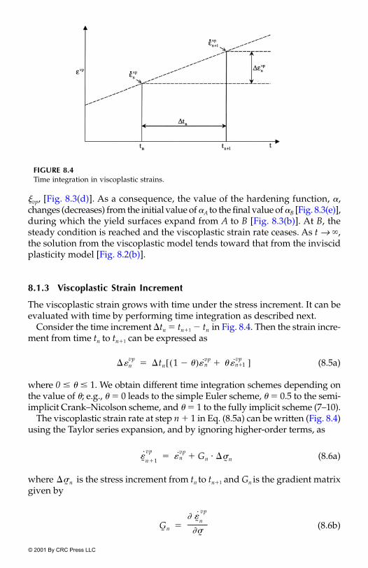
© 2001 By CRC Press LLC
�vp, [Fig. 8.3(d)]. As a consequence, the value of the hardening function, ,changes (decreases) from the initial value of A to the final value of B [Fig. 8.3(e)],during which the yield surfaces expand from A to B [Fig. 8.3(b)]. At B, thesteady condition is reached and the viscoplastic strain rate ceases. As t → �,the solution from the viscoplastic model tends toward that from the inviscidplasticity model [Fig. 8.2(b)].
8.1.3 Viscoplastic Strain Increment
The viscoplastic strain grows with time under the stress increment. It can beevaluated with time by performing time integration as described next.
Consider the time increment �tn � tn�1 � tn in Fig. 8.4. Then the strain incre-ment from time tn to tn�1 can be expressed as
(8.5a)
where 0 � � � 1. We obtain different time integration schemes depending onthe value of �; e.g., � � 0 leads to the simple Euler scheme, � � 0.5 to the semi-implicit Crank–Nicolson scheme, and � � 1 to the fully implicit scheme (7–10).
The viscoplastic strain rate at step n � 1 in Eq. (8.5a) can be written (Fig. 8.4)using the Taylor series expansion, and by ignoring higher-order terms, as
(8.6a)
where is the stress increment from tn to tn�1 and Gn is the gradient matrixgiven by
(8.6b)
FIGURE 8.4Time integration in viscoplastic strains.
��nvp
�tn 1 ��( )� nvp ��n 1�
vp�[ ]�
�˜ n�1
vp�n
vp Gn ��˜ n���
��˜ n
G˜ n
�˜ n
vp
�˜
-------------�

© 2001 By CRC Press LLC
Then, based on Eq. (8.2d), F, and �, Gn is derived as
(8.6c)
The substitution of Gn in Eq. (8.5a) leads to
(8.5b)
8.1.4 Stress Increment
The stress increment is written as
(8.7a)
where � , is the strain-displacement transformation matrix, is the displacement vector, and is the elastic constitutive matrix.
Now, substitution of from Eq. (8.5b) in Eq. (8.7a) gives
(8.7b)
(8.7c)
where , and is the time-dependent,equivalent “elastic” strain.
8.1.5 Elastoviscoplastic Finite-Element Equations
In the evp approach, we solve the equations of equilibrium below, by per-forming time integration for strains for a given load increment, (n � 1,2,…); see Fig. 8.5. The finite-element incremental equations of equilibrium arewritten as
(8.8a)
where V is the volume of finite element. Now, substitution of Eq. (8.7b) in Eq.(8.8a) gives
(8.8b)
G˜ n � �
�
˜
------- F�
˜
-------
T d�dF------- F
�˜
------- F�
˜
-------
T
��
�
��˜ n
vp�tn [ �
˜nvp
� Gn��˜ n]���
��˜ n C
˜ ne
��˜ n
��˜ n
vp�( )�
��˜ n
B˜ n�q
˜n
B˜
q˜
nC˜
e
��nvp
��˜ n C
˜B˜ n �q
˜n
� nvp
�tn���( )�
C˜
��˜
e t( )��
C˜
I˜
C˜ n
e� � �tn G
˜ n� � �( ) 1�C˜ n
e� ��
˜e t( )
�Q˜
n
B˜ n
T��
˜ ni V �Q
˜n�d
V� 0�
B˜ n
TC˜
B˜ n�qn �n
vp�tn�( )dV �Q˜
n�V
� 0�

© 2001 By CRC Press LLC
or
(8.8c)
or
(8.8d)
where is the tangent stiffness matrix given by
(8.9)
and is the equivalent, residual, or pseudo-incremental load vector, givenby
(8.10)
Once the increment of displacement is computed by solving Eq. (8.8d),the increment of stress can be found from Eq. (8.7b). Then the total quan-tities at step n � 1 are found as
(8.11a)
(8.11b)
FIGURE 8.5Incremental loading in evp solution.
B˜ n
TC˜
B˜ n dV( )�q
˜n
B˜ n
TC˜
�nvp�tn dV
V�� �Q
˜n�
V� 0�
�q˜
nk˜ t n( )
�1 B˜ n
TC˜
�nvp�tn dV� �Q
˜n�
V��
k˜ t n( )
�1�Q
˜�
k˜ t n( )
�1
k˜ t n( ) B
˜ nTC
˜B˜ n dV
V��
�Q˜
�Q˜
B˜ n
TC˜
� nvp
�tn dV� �Q˜
n�V
��
�q˜
n��
˜n
q˜
n�1q˜
n�q
˜n
��
�˜ n�1 �
˜ n ��˜ n��

© 2001 By CRC Press LLC
Now the increment of viscoplastic strain, , is found using Eq. (8.7a):
(8.12a)
and the total quantity is
(8.12b)
Then Eq. (8.6a) is used to evaluate the viscoplastic strain rate for the timeinterval �tn [Fig. (8.4)]. When the strain rate becomes small, as in Fig. 8.3, thetime integration process is stopped. The next load increment, , isapplied and the process is repeated.
8.1.6 One-dimensional Formulation of Perzyna (evp) Model
The rheological model for the uniaxial case is shown in Fig. 8.6 (7, 16). The springand dashpot provide for (linear) elastic and viscous responses, respectively. Theslider provides the plastic yielding response depending on the plasticity model(F) adopted (Chapters 6 and 7). Under a given stress (increment), �, at time t � 0,the instantaneous elastic response, , is given by
(8.13)
where E is the elastic modulus of the linear spring. Note that at time t � 0, thedashpot and the slider are not operational; however, for t 0, the dashpotand the slider become operational. The slider will move only after the stressin it, �s, becomes greater than the yield stress, �y. The excess or overstress, �d,in the dashpot is given by
(8.14)
FIGURE 8.6Elastoviscoplastic (evp) model.
��nvp
��nvp B
˜ n�q˜
nC˜
e( )�1��
˜ n��
�˜ n�1
vp�˜ n
vp�˜ n
vp��
�Q˜
n�1
�e
�e �
E---�
�d � �s��

© 2001 By CRC Press LLC
The initiation of viscoplastic strains will take place after the yield stress, �y ,is induced in the slider. Hence, the stress, , for linear strain-hardeningresponse (Fig. 8.7), during which viscoplastic strains occur, is given by
(8.15)
where H� is the slope of the linear strain-hardening part of the stress–straincurve. Then the stress in the slider is given by
(8.16)
Now the total strain, �, is given by
(8.17)
where is the elastic strain, and the stress in the dashpot, �d, is given by
(8.18)
where � is the coefficient of viscosity and t is the time. Before yielding, � 0,therefore, �d � 0 [Eq. (8.18)], and hence �s � � [Eq. (8.14)].
Substitution of Eqs. (8.15), (8.16), and (8.18) in Eq. (8.14) gives
(8.19)
FIGURE 8.7Elastic linear, strain-hardening, stress–strain behavior: uniaxial case (7, 16) (with permission).
�
� �y H��vp
��
�s
� if �s ��
� if �s ��
�
� �e
�vp
��
�e
�d �d�
vp
dt----------�
�vp
�d�
vp
dt---------- H��
vp�y� � ��

© 2001 By CRC Press LLC
and substitution of , Eq. (8.17), with Eq. (8.13), in Eq. (8.19) leads to
(8.20a)
which represents a first-order ordinary differential equation for the time-dependent relation between stress and strain. Equation (8.20a) can be writtenin terms of the fluidity parameter, �, as
(8.20b)
where � � 1/�.
(8.21)
Comparing Eqs. (8.21) and (8.20b), we have
(8.22)
Here, � � (�y � H� ) denotes the overstress that causes viscoplastic strains;in other words, in this model, the viscoplastic strain rate is defined uniquelyin terms of the overstress.
We can obtain the closed-form solution to Eq. (8.20a) for a constant-appliedstress �. Equation (8.20a) can now be written as
(8.23)
The solution to Eq. (8.23) is given in (7, 16) as
(8.24)
where H� 0. Figure 8.8(a) shows a schematic of the solution in Eq. (8.24). Itshows that the instantaneous elastic strain, � , will be followed by thetime-dependent viscoplastic strains, whose limiting value will be (� � �y)/H� ast → � [Eq. (8.24)], which is the same as the plastic strain from inviscid plasticity.
For an elastic perfectly plastic material (H� � 0), the solution is obtained byusing l’Hospital’s rule such that H� → 0 (7):
(8.25)
�vp
H�E� �E d�dt------� H�� E � �y�( ) �
d�dt-------� ��
��E--- � � �y H��
vp�( )�[ ]��
� �e
�vp
��E--- �
vp�� �
�vp
� � �y H��vp
�( )�[ ]�
�vp
�H��d�dt------�
�H�E
-----------� � � �y�( )��
��E---
� �y�
H�----------------- 1 e H��t�
�( )��
�e
� E�
��E--- � �y�( )�t��

© 2001 By CRC Press LLC
Figure 8.8(b) shows a plot of the solution, Eq. (8.25). It can be seen that forthe perfectly plastic material, the steady-state condition for is not reached,and can continue indefinitely at a constant strain rate.
It may be noted that the model in Eq. (8.24) for a strain-hardening materialleads to the equilibrated or steady-state viscoplastic strain, which is the sameas the corresponding plastic strain from the inviscid plasticity (Chapter 7)[Fig. 8.2(b)]. Thus, the Perzyna model provides the timewise variation of theirreversible or plastic strain; however, its final magnitude is the same as thatfrom the plasticity model based on the given yield function, F.
Details of the one-dimensional model for stress relaxation are given inExample 8.10.
FIGURE 8.8Responses of evp model: uniaxial case.
�vp
�vp

© 2001 By CRC Press LLC
8.1.7 Selection of Time Step
The robustness and reliability of the solution based on the time integrationscheme, Eq. (8.5), depends on the selection of the appropriate size of the timestep, �t. For � � 0.5, it has been shown [Hughes and Taylor (17)] that the schemein Eq. (8.5) is unconditionally stable. However, stability may not necessarilyimply accuracy of the solution, and it thus becomes necessary to limit the size ofthe time step.
The size of the time step is affected by a number of factors such as materialproperties and strain rate. An empirical relation between the time step sizeand strain rate proposed by Cormeau (2), Zienkiewicz and Cormeau (3), andDinis and Owen (18) for the explicit integration is given by
(8.26)
where � is a problem-dependent parameter whose value can be in the range0.01 � � � 0.15. It is often economical to vary the time step size during thetime integration. One such empirical formula is given by Zienkiewicz andCormeau (3):
(8.27)
where 1.2 � �0 � 2. Owen and Hinton (7) have given time-size criteria for var-ious yield functions such as Tresca, von Mises, and Mohr–Coulomb for theassociated flow rule.
8.2 Disturbance Function
The DSC model can be developed using the constitutive incremental equationsfor the evp model so as to characterize the RI behavior. Figure 8.9(a) shows aschematic of stress–strain behavior from a creep test in which increments ofstress are applied at a slow rate, and the steady viscoplastic strains are measuredunder the constant values of increments. Such a behavior is referred to as a staticresponse. The hardening curve in Fig. 8.9(a) shows the locus of the stresses andsteady-state strains, which are the same as that for inviscid plasticity response.The observed (a) stress–strain response, Fig. 8.9(a), may exhibit degradation andsoftening. Then the static hardening response can be treated as RI, and the FA (c)response can be identified on the basis of the asymptotic stress states (Chapter 4).The disturbance, D, can now be defined as (Chapter 4)
(8.28a)
�t ��
� vp-------�
�
� vp-------
�E--- �
vp�
�
�tn 1� �0�tn�
D�
i�
a�
�i
�c
�------------------�

© 2001 By CRC Press LLC
where denotes a measure of stress such as � or , is the observedstress, and is the FA stress.
For cyclic (repetitive) loading [Fig. 8.9(b)], the disturbance treated as thefunction of �(N), where N is the number of cycles, can be expressed as
(8.28b)
where �p is the peak stress for a given cycle N. D in Eq. (8.28b) can beexpressed in terms of a viscoplastic (deviatoric) strain trajectory, Eq. (8.4c). Inthe case of cyclic loading, the RI behavior can be simulated using the inviscidplasticity model, say, �0,Chapter 7, by using the initial and monotonicresponse of the first cycle, extended beyond the peak point; see Fig. 8.9(b).
FIGURE 8.9Disturbance for creep models.
�i J2D �
a
�c
D N( )�
i�p�
�i
�c
�------------------�

© 2001 By CRC Press LLC
Now the observed stress increment, , can be expressed as
(8.29)
where is the intact viscoplastic stress increment as given in Eq. (8.7b). Ifit is assumed that the strains (t) [Eq. 8.7(c)] in the RI and FA parts areequal, Eq. (8.29) can be written as
(8.30a)
(8.30b)
where is the constitutive matrix for the FA response and will depend onthe simulation used (Chapter 4). For example, for the constrained-liquidassumption, in Eq. (8.30) will specialize to Eq. (4.19) in Chapter 4.
8.2.1 Finite-Element Equations
The equilibrium equations (8.8a) can now be written as
(8.31)
Substitution from Eq. (8.30) in Eq. (8.31) and the use of Eq. (8.7b) leads to
(8.32a)
or
(8.32b)
where
��˜
a
��˜
a 1 D�( )��˜
i D��˜
c dD �˜
c�˜
i�( )���
��˜
i
��˜
e
��˜
a 1 D�( )C˜
��˜
e DC˜
c��
˜e dD �
˜c
�˜
i�( )� ��
1 D�( )C˜
DC˜
c�[ ]��
˜e dD �
˜c
�˜
i�( )��
C˜
c
C˜
c
B˜ n
T��
˜ na V �Q
˜n�d� 0�
B˜ n
T 1 D�( )C˜
DC˜
c�{ } B
˜ n�q˜
n
i� n
vp�nt
�{ } dD �˜
c�˜
i�( )�[ ] Vd �Q
˜n�
V� 0�
k˜ t
DSC�q
˜n
i Q˜
1 Q˜
2� �Q˜
n��� �Q˜
DSC�
ktDSC B
˜ nT 1 D�( )C
˜DC
˜c
�[ ]B˜ n Vd
V��
Q˜
1 B˜ n
T 1 D�( )C˜
DC˜
c�[ ]� n
vp�tn VdV
��
Q˜
2 B˜ n
TdD �˜
c�˜
i�( ) Vd
V��

© 2001 By CRC Press LLC
and is the equivalent or residual load vector including the effect of dis-turbance.
8.3 Rate-Dependent Behavior
The behavior of most engineering materials depends on the rate of loading(Fig. 8.10), which is often defined by strain rate, , or displacement rate, The static response refers to the behavior under a slow rate of loading. As theloading rate increases, the material exhibits stiffer response and higher ulti-mate or failure strengths; Fig. 8.10(a) and (b) show schematics of such behav-ior at a given initial (continuing) stress or mean pressure. Hence, there existsa unique ultimate envelope corresponding to each strain rate. It is possiblethat a material may exhibit hardening response under static loading. How-ever, if it is loaded under variable strain rates (under dynamic loading) inwhich the strain rate decreases after an increasing strain rate, the materialmay exhibit strain softening behavior (5) [Fig. 8.10(c)].
FIGURE 8.10Rate-dependent behavior (5). ©1984 John Wiley & Sons Ltd. Reproduced with permission.
�Q˜
DSC
� �.

© 2001 By CRC Press LLC
The evp model can be used for the strain rate-dependent behavior. In thiscase, the dynamic yield surface, Fd, will depend on the rate of loading. In otherwords, if the same stress increment is applied at different rates, the dynamicyield surface, Fdi (i � 1, 2, …) [Fig. 8.10(d)], � will be different. However, theprocedures for the evaluation of the viscoplastic strain and for the conver-gence of Fd → 0 to the equilibrated yield surface (Fs � 0) for the stress incre-ment will be essentially the same as before.
8.4 Parameters for Elastoviscoplastic (evp) Model
The procedures for finding the elasticity and plasticity constants have beendescribed in Chapters 5 to 7. For example, if the �0-model in the HISS familyis used, the parameters involved are those discussed in Chapter 7. Here weconsider the parameters required for the viscous behavior in the evp model.
8.4.1 Determination of Parameters
There are two parameters, � [Eq. (8.2d)] and N or [Eq. (8.3)], that need tobe determined from appropriate laboratory tests.
Fluidity Parameter, �. Squaring both sides of Eq. (8.2d) and multiplyingthem by 1�2 leads to
(8.33a)
or
(8.33b)
where is the second invariant of the viscoplastic strain rate tensor, .Therefore,
(8.34a)
where
(8.34b)
N
12--- �
˜vp( )
T�˜
vp 12--- � �⟨ ⟩( )2 F
�˜
-------
T F�
˜
-------�
I2vp 1
2--- � �⟨ ⟩( )2 F
�˜
-------
T F�
˜
-------�
I2vp
�˜
vp
� �⟨ ⟩ 2 I2vp
F�
˜
------- T F
�˜
------------------------- a� �
F�
˜
------- FJ1-------I
˜F
J2D-----------S
˜F
J3D----------- S
˜T S
˜
23--- J2DI
˜��
� ��

© 2001 By CRC Press LLC
is the vector of deviatoric stresses, and the invariant, I2, is given by
(8.34c)
in which �ij is the strain tensor.The value of a in Eq. (8.34a) can be found for various points during a creep
test. Although the applied overstress, is constant in a creep test, the yieldfunction (Fd 0) changes during the creep behavior because the viscoplasticstrain rate, Eq. (8.6a), leads to changes in the hardening function, , Eq. (8.4b),with the viscoplastic strain trajectory, �vp, Eq. (8.4c). As the strains are meas-ured during the test, the values of can be found for various points.
The flow function, �, as power law is given by Eq. (8.3b) as (2, 3, 7–12)
(8.35a)
Now Eq. (8.34a) is written as
(8.35b)
Therefore,
(8.35c)
Variation of a vs. F/F0 is shown (schematically) in Fig. 8.11(a), whereas in theln–ln plot it is shown in Fig. 8.11(b). The slope of the (average) straight linegives N, and the intercept when F/F0 � 1 gives �.
Other forms of the flow function are possible, e.g., the exponential form isgiven by (2–4, 7–10, 16) [Eq. (8.3c)]:
(8.36a)
Then Eq. (8.34a) leads to
(8.36b)
Therefore,
(8.36c)
S˜
I212---�ij�ij
12---tr �( )2
� �
�˜
,
I2vp
�FF0-----
N
�
� � FF0-----
N
� a�
ln � Nln FF0-----
� ln a�
�FF0-----
expN
1.0��
�FF0-----
expN
1.0� a�
ln �FF0-----
N� ln a�

© 2001 By CRC Press LLC
The values of � and are found from a plot of ln� vs. F�F0 evaluated at dif-ferent points on the creep curve.
8.4.2 Disturbance Parameters
Procedures for the determination of the disturbance parameters, A, �, and Du,are described in Chapters 2 and 4. For quasistatic (one-way loading andunloading), results such as in Fig. 8.9(a) can be used with Eq. (8.28a). Forcyclic loading [Fig. 8.9(b)], D can be found using Eq. (8.28b). Consider the dis-turbance given by (Chapter 3)
(8.36c)
Here, Du can be found using Eq. (8.28a) or (8.28b) in which , is the residualor saturation stress after a large number of cycles. Often, it is appropriate touse Du � 1.0. The values of D at different stress levels are found, and � isfound from viscoplastic strains at those points. Then plot of ln[�ln(1 � D)]vs. ln(�vp) provides the values of A and Z (Chapter 3).
FIGURE 8.11Determination of creep parameters.
N
D Du 1 eA�D
Z�
�( )�
�c

© 2001 By CRC Press LLC
8.4.3 Laboratory Tests and Examples
One-dimensional. Usually, results are available from tests with one-dimensional constant stress and�or constant strain loading. For instance,steady-state (uniaxial) creep strain rate ( ) vs. uniaxial stress (�1) results areoften available. Figure 8.12(a) shows such temperature-dependent data for a60�40 (Sn/Pb) solder (11, 19), which can be used to find approximate values of� and N. Here, because only one component of strain is available, Eq. (8.2d)reduces to
(8.37a)
which leads to
(8.37b)
The values of F can be found from Eq. (8.4a) as the state of stress and other (plas-ticity) material parameters are known. Here, F0 � pa is used. Typical plots ofln( ) vs. ln (F�F0) for different temperatures are shown in Fig. 8.12(b) (11); thetemperature dependence is discussed later. The slope of an average line gives thevalue of N and the intercept along ln( ) for F/F0 � 1, that is, ln(F/F0) � 0 givesthe value of �.
Shear Tests. For geologic and other materials, shear tests are often per-formed, in which the specimen is first consolidated under the K0 condition,i.e., lateral strain � 0. After the consolidation, the specimen is subjected to a
FIGURE 8.12Plots of measured (a) strain rate vs. stress (19), and (b) ln(F/F0) vs. ln for determinationof � and N (11).
� 1vp( )
�vp
� 1
˙vp�
FF0-----
N
�
ln � 1vp ln� Nln F F0�( )��
� 1vp
� 1vp

© 2001 By CRC Press LLC
constant effective normal stress, � , and a constant shear stress, �, isapplied under undrained conditions; that is, the fluid is not allowed to drain.The shear strains are measured with time under the constant �. For this un-drained case, the vertical strain, �1, is zero. Then the viscoplastic strain ratetensor is given by
(8.38)
FIGURE 8.12(Continued).
��n ��3
�vp
( )0 0 00 0 � 2�0 � 2� 0
�
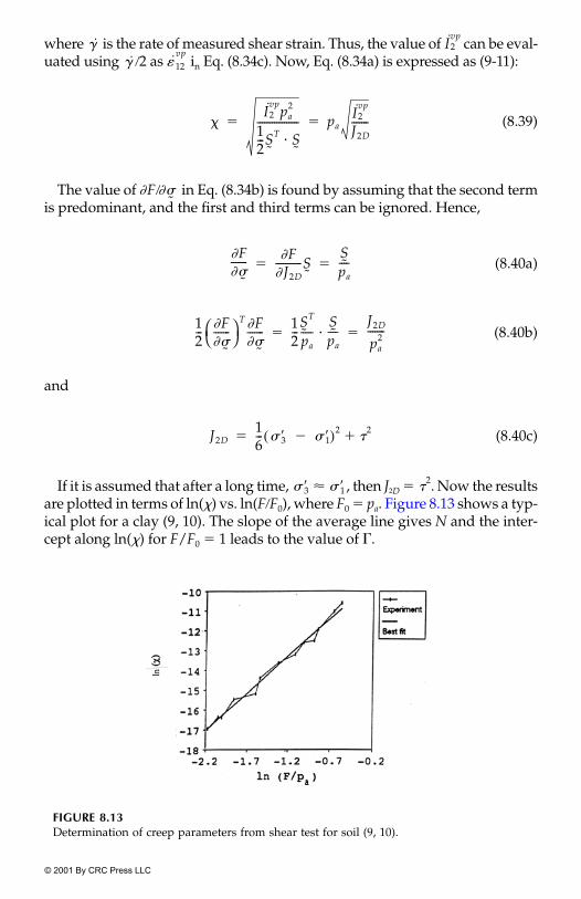
© 2001 By CRC Press LLC
where is the rate of measured shear strain. Thus, the value of can be eval-uated using �2 as in Eq. (8.34c). Now, Eq. (8.34a) is expressed as (9-11):
(8.39)
The value of in Eq. (8.34b) is found by assuming that the second termis predominant, and the first and third terms can be ignored. Hence,
(8.40a)
(8.40b)
and
(8.40c)
If it is assumed that after a long time, � , then J2D � . Now the resultsare plotted in terms of ln(�) vs. ln(F�F0), where F0 � pa. Figure 8.13 shows a typ-ical plot for a clay (9, 10). The slope of the average line gives N and the inter-cept along ln(�) for F/F0 � 1 leads to the value of �.
FIGURE 8.13Determination of creep parameters from shear test for soil (9, 10).
� I2vp
� � 12vp
�I2
vppa
2
12---S
˜T S
˜�
----------------- paI2
vp
J2D-------� �
F �˜
�
F�
˜
------- FJ2D-----------S
˜
Spa----� �
12--- F
�˜
-------
T F�
˜
------- 12---
S˜
T
pa-----
Spa----�
J2D
pa2
-------� �
J2D16--- ��3 ��1�( )2
�2
��
��3 ��1 �2

© 2001 By CRC Press LLC
8.4.4 Temperature Dependence
The temperature (T) dependence can be introduced in the viscoplastic modelby writing Eq. (8.2d) for associated flow (Q � F) as
(8.41)
where is the thermoviscoplastic strain rate tensor, F (�ij, , T ) is the tem-perature-dependent yield function, and �(T) is the temperature-dependentfluidity parameter.
As discussed earlier, the rate of increase in the thermoviscoplastic strain isaffected by the excess stress above the yield stress as well as by the tempera-ture, which may result in thermal degradation. Assuming that the viscousbehavior is exhibited after the passage to the transient thermoviscoplasticstate and that it is not significant in the elastic region, the total strain rate, ,can be expressed in terms of the thermoelastic strain rate, , thermoviscoplas-tic strain rate, , and the elastic contribution due to the coefficient of ther-mal expansion ( T) effect as
(8.42a)
or
(8.42b)
The constitutive stress–strain equation can now be written as
(8.43)
The thermoviscoplastic strain rate at time step n � 1 is now expressed usingTaylor series (ignoring higher-order terms) as
(8.44a)
(8.44b)
where is the stress increments and and are the gradient matrices
�˜
vpT( ) � T( ) � F( )⟨ ⟩ F
�˜
-------�
�˜
vp
ij T( )
�˜�
˜e
�˜ i j
vpT( )
�˜
T( ) �˜
eT( ) �
˜vp T( ) T T( )TI
˜� ��
�˜
T( ) �˜
eT( ) � T( )��
FF0-----
�F�
˜
------- T T( )TI˜
� ��
�˜˙ C
˜e T( ) �
˜T( ) � T( )��
FF0-----
�F�
˜
-------� TTI˜
��
�˜ n�1
vp T( ) �˜ n
vp T( ) �
˜ n
vp
�˜
------------- ��n� �
˜ n
vp
T------------- �TnI
˜�� ��
�˜ n
vp T( ) G˜ n1��
˜ n Gn2�TnI˜
� ��
��˜ n G
˜ n1 Gn2
© 2001 By CRC Press LLC
at step n, given by
(8.45a)
and
(8.45b)
where
and
Here, the exponent, N, can depend on the temperature, T.
8.5 Multicomponent DSC and Overlay Model
The evp model based on Perzyna’s theory simulates the viscoplastic response,particularly the time-dependent plastic response during the secondary creepregime (Fig. 8.1). However, in general, a material may experience both vis-coelastic and viscoplastic responses, which include creep deformation duringboth the primary and secondary creep regimes. Hence, it is appropriate todevelop and use a model that can simulate the combined response as closelyas possible. In the following, we develop a model, called viscoelastic-visco-plastic (vevp), that can allow consideration of the combined response. Vis-coelastic (ve) and elastoviscoplastic (evp) models arise as special hierarchicaloptions of the vevp model.
8.5.1 Multicomponent DSC
In the basic DSC (Chapters 2 and 4), we first considered an element of thesame material, which is composed of two material parts in the RI and FA ref-erence states. During deformation, the extents of the RI and FA parts change,which is defined through the disturbance, D. In Chapter 2, we also developedthe DSC for a material element composed of more than one or two, or a
G˜ n1
�˜
vpT( )
�˜
---------------------- �
F-------- F
�˜
-------� F
�˜
------- �
2F�
˜2
---------�� �
G˜ n2
�˜
vpT( )
T----------------------
� T( )�F------- F
T-------� �
F�
˜
-------� � �� T( )
T----------------
F�
˜
-------��
� � T( )�, and � = FF0-----
N T( )�
�F-------- � T( )N T( )
F0-------------
FF0-----
N 1�
�

© 2001 By CRC Press LLC
higher number of, different materials. In that case, the behavior of the com-ponent materials provide reference state responses. Then the observed stress,
, can be expressed as
(8.46)
where A1, A2, …, An are the areas of the components (Fig. 8.14), with total areaA � �Ai (i � 1, 2, …, n), and , , …, are the corresponding stresses. Forconvenience, we assume that the width of the material element is constantand equals b (Fig. 8.14). Equation (8.46) can be written as
(8.47)
where di � Ai�A is the ratio of the area of component i to the total area A; here,�di � 1. Note that Eq. (8.47) is similar to that for the single material elementwith RI and FA parts in which the disturbance, D, is the ratio of the FA areato the total area, i.e., D � �A. In the basic DSC, Di (i � 1, 2) varies with
FIGURE 8.14Multicomponent DSC.
�a
�a
�1A1
A------ �
2A2
A------ … �
nAn
A------� � ��
�1
�2
�n
�a
�1d1 �
2d2… �
ndn� � ��
Ac

© 2001 By CRC Press LLC
deformation, while in the multicomponent DSC, di(i � 1, 2, …, n) can be con-stant. Equation (8.47) can also be expressed as
(8.48a)
or
(8.48b)
where b � width of the element and t1, t2, . . . , tn (� ti/�ti) are the nondimen-sionalized thicknesses of the components of the material element (Fig. 8.14);hence, �ti � 1. Then each component (i � 1, 2, . . . , n) of the material elementcan be characterized using different models such as elastic, viscoelastic, andelastoviscoplastic.
The three-dimensional incremental form of Eq. (8.48) can be written as
(8.49a)
(8.49b)
As indicated before, di do not change and hence, ti also do not change duringsmall deformation. Equation (8.49a) can now be written as
(8.50)
where (m � 1, 2, …, n) are the (tangent) constitutive matrices for the com-ponents, and (m � 1, 2, …, n) are the corresponding incremental strainvectors, which, in general, can be different. If it is assumed that the strains inall components are equal (� ), Eq. 8.50 becomes
(8.51a)
or
(8.51b)
where is the equivalent constitutive matrix for the material element.Figure 8.14(b) shows a symbolic representation of the multicomponent DSCmodel from Eq. (8.51). Each component unit (1, 2, …, n) can be characterizedusing elastic, viscoelastic, elastoviscoplastic, or any appropriate model. Thus,it can provide a hierarchical framework from which elastic (e), viscoelastic (ve),
�a
�1 t1b�tib---------- �
2 t2
�ti-------b
b-- … �
n tn
�ti-------b
b--� � ��
�a
�1t1 �
2t2… �
ntn� � ��
d�˜
a d�˜
1t1 d�˜
2t2… d�
˜ntn� � ��
d�˜
jt jj 1�
n
��
d�˜
a t1C˜
1d�˜ 1
t2C˜
2d�˜ 2
… tnC˜
nd�˜ n
� � ��
C˜
m
d�m
d�
d�˜
a t1C˜ 1
1 t2C˜ 2
2 … tnC˜
� � �( )d�˜
�
d�˜
a C˜ eq d�
˜�
C˜ eq

© 2001 By CRC Press LLC
elastoviscoplastic (evp), and viscoelasticviscoplastic (vevp) models can beextracted. Note that the evp model can be the same as that discussed earlier,based on the Perzyna theory. The special form, Eq. (8.51), with compatiblestrains of the multicomponent DSC model, Eq. (8.50), is the same as the over-lay or mechanical sublayer model proposed and used in (7, 20–22).
A rheological representation of the overlay model considered here is shownin Fig. 8.15(b), while that for the elastoviscoplastic (evp-Perzyna) model isshown in Fig. 8.15(a), as a special case. By adopting a suitable number of over-lays with different thicknesses such that �ti(i � 1, 2,…,k) � 1, and by assigningdifferent material properties such as elasticity (E, ν), plasticity (perfectly plas-tic, �y; �0-plasticity, �, �, a1, �1, n, 3R, etc.), and viscous (�, N) to different rheo-logical units, a wide range of special versions can be obtained. Table 8.1 showsa number of possible versions, whose explanations follow.
Elastic (e). For the single unit, Fig. 8.15(a), consider one overlay with thick-ness t � 1. The spring and dashpot are assigned elastic (E, ν) and viscous (�, N)parameters, respectively, while the yield stress, �y , in the slider, as per vonMises, perfectly plasticity model is assigned a very high value, of the order of
(Table 8.1). Then, as �y is very high, the dashpot will not be operational,and only the elastic spring will operate, which will result in an elastic response.
TABLE 8.1
Specializations of Overlay Model
SpecializationPlasticity
ModelNo. of
Overlays Thickness Parameters
Elastic (e) von Mises 1 1.0 E, ν, �, N, and very high �yMaxwell von Mises 2 0.5, 0.5 E1, ν1, �1, N1, �y1 � 0
E2, ν2, �2, N2, �y2 � 0Viscoelastic (ve) von Mises 2 0.5, 0.5 E1, νv1, �1, N1, �y1 � 0
E2, ν2, �2, N2, �y2 �
very highElastoviscoplastic(evp) (Perzyna type)
Any 1 1.0 E, ν, �, N, F
Viscoelasticvisco-plastic (vevp)
von Mises 0.5 E1, ν1, �1, N1, �y1 � 0
Any 0.5 E2, ν2, �2, N2, �y2, or F
FIGURE 8.15Overlay model and elastoviscoplastic specialization.
11
2�
108

© 2001 By CRC Press LLC
Maxwell Model. Here, two units with thickness each equal to 0.50 can beused. Then adoption of the yield stress, �y1 � �y2 � 0.0, leads to two parallelMaxwell models with spring and dashpot in series.
Viscoelastic (ve). Consider the two units from Fig. 8.15(b), with two over-lays with t � 0.5 each. Units 1 and 2 are assigned the properties as shown inTable 8.1. Because of the very high value of �y2, the dashpot in unit 2 will notoperate, and because �y1 � 0 in unit 1, only the spring and dashpot will oper-ate; the effective model is shown in Fig. 8.16(a). At time t � 0, under a stress of�0, instantaneous elastic strain, will occur because of the springs in units 1and 2, given by
(8.52)
For time t 0, viscoelastic deformations will occur due to the operation ofthe dashpot in unit 1 [Fig. 8.16(b)]. Then, if the stress is removed, the elasticstrain will be recovered first instantaneously, and then � → 0, as t → �, becausethe elastic spring in unit 2 will force the dashpot to return to the original state.Thus, this specialization will yield viscoelastic response.
Elastoviscoplastic (evp)—Perzyna Model. We consider one unit, Fig. 8.15(a),and one overlay with thickness t � 1. The elastic (E, ν), viscous (�, N), and �y
(classical plasticity) or F (e.g., �0-model) are assigned to the spring, dashpot,and the slider, respectively (Table 8.1).
At time t � 0, the dashpot will not be operational; hence, the instanta-neous elastic strain, � �0/E, will occur. Then, for time t 0, the dashpotwill be operational, and viscoplastic strains will occur. On unloading, willbe recovered, and the viscoplastic strains ( ), [Fig. 8.17(b)], due to theslider (�y or F) [Fig. 8.17(a)], will remain. The final viscoplastic strain will beequal to that from inviscid plasticity governed by the yield function, F. Inother words, the evp-type model will give the timewise variation of theplastic strains, but the final magnitude of the viscoplastic will be equal tothe plastic strain from inviscid plasticity.
FIGURE 8.16Viscoelastic model.
�e,
�e �0
E1t1 E2t2�----------------------------�
�e
�e
��p

© 2001 By CRC Press LLC
Viscoelasticviscoplastic (vevp) Model. Consider the two units in themodel, Fig. 8.15(b), and assume two overlays, each with thickness � 0.5. Theparameters are assigned as shown in Table 8.1. The resulting model is shownin Fig. 8.18(a).
At time t � 0, only the springs will deform as the dashpots are not opera-tional. The instantaneous elastic strain [0–A, Fig. 8.18(b)], will be given byEq. (8.52). Then, for time t 0, the dashpot in unit 1 will operate first, as theslider in unit 2 has nonzero yield stress. This will lead to viscoelastic deforma-tions. Now for later time t 0, when the yield condition in slider 2 is reached,the dashpot in unit 2 will also become operational. If continuous yielding (e.g.,�0-model) is considered for the slider, both the viscoelastic and viscoplasticdeformations can occur simultaneously during A–B. Upon unloading, willbe recovered first, then the viscoplastic strain, , will be recovered, andfinally the viscoplastic strain will remain [Fig. 8.18(b)].
FIGURE 8.17Elastoviscoplastic model.
FIGURE 8.18Viscoelasticviscoplastic model.
�e
�e
�ve
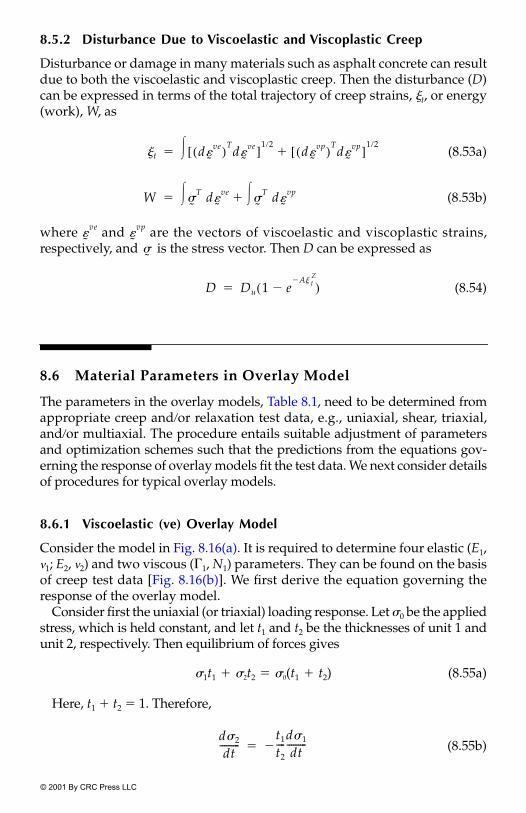
© 2001 By CRC Press LLC
8.5.2 Disturbance Due to Viscoelastic and Viscoplastic Creep
Disturbance or damage in many materials such as asphalt concrete can resultdue to both the viscoelastic and viscoplastic creep. Then the disturbance (D)can be expressed in terms of the total trajectory of creep strains, �t, or energy(work), W, as
(8.53a)
(8.53b)
where and are the vectors of viscoelastic and viscoplastic strains,respectively, and is the stress vector. Then D can be expressed as
(8.54)
8.6 Material Parameters in Overlay Model
The parameters in the overlay models, Table 8.1, need to be determined fromappropriate creep and�or relaxation test data, e.g., uniaxial, shear, triaxial,and�or multiaxial. The procedure entails suitable adjustment of parametersand optimization schemes such that the predictions from the equations gov-erning the response of overlay models fit the test data. We next consider detailsof procedures for typical overlay models.
8.6.1 Viscoelastic (ve) Overlay Model
Consider the model in Fig. 8.16(a). It is required to determine four elastic (E1,ν1; E2, ν2) and two viscous (�1, N1) parameters. They can be found on the basisof creep test data [Fig. 8.16(b)]. We first derive the equation governing theresponse of the overlay model.
Consider first the uniaxial (or triaxial) loading response. Let �0 be the appliedstress, which is held constant, and let t1 and t2 be the thicknesses of unit 1 andunit 2, respectively. Then equilibrium of forces gives
�1t1 � �2t2 � �0(t1 � t2) (8.55a)
Here, t1 � t2 � 1. Therefore,
(8.55b)
�t d�˜
ve( )Td�
˜ve[ ]
1�2d�
˜vp( )T
d�˜
vp[ ]1�2
���
W �˜
T d�˜
ve� �˜
T d�˜
vp���
�˜
ve�˜
vp
�˜
D Du 1 eA� t
Z�
�( )�
d�2
dt---------
t1
t2----
d�1
dt---------��

© 2001 By CRC Press LLC
At time t � 0, the dashpot is not operational; hence, the strain �0 is givenby
(8.56)
Now, with respect to unit 1:
(8.57a)
where and are the strains in the spring and dashpot, respectively.Hence,
(8.57b)
where �1 is the stress in unit 1.With respect to unit 2:
(8.58a)
Hence, using Eq. (8.55b),
(8.58b)
Combining Eqs. (8.57b) and (8.58b), we have
(8.59)
the solution of which can be obtained as
(8.60)
where a � E1E2t2, b � E1t1 � E2t2. Therefore,
(8.61a)
�0
E1t1 E2t2�---------------------------- and �1 0( )
E1�0
E1t1 E2t2�----------------------------�
� �e
�d
��
�e
�d
d�dt------ 1
E1-----
d�1
dt--------- ��1��
��2
E2-----�
d�dt------
1E2-----�
t1
t2----
d�1
dt---------�
1E1-----
t1
t2---- 1
E2-----�
d�1
dt--------- ��1� 0�
�1 �1 0( ) et�a�b
--------------��
d�1
dt--------- �1 0( ) t�a�
b--------------e
t�a�b
--------------�

© 2001 By CRC Press LLC
and from Eq. (8.55b):
(8.61b)
Substitution of Eq. (8.61a) in Eq. (8.58b) gives
(8.62a)
Integration of Eq. (8.62a) leads to the solution for the overlay strain, �, as
(8.62b)
As indicated before, the parameters E1, E2, and � can be found by their suit-able adjustment, such that the computed strains � for given �0 fit the observedresponse. They can be obtained by using the following simplified procedure:
For t � 0, Eq. (8.62b) gives
(8.63a)
As t → �, Eq. (8.62b) gives the ultimate strain, �u, as
(8.63b)
The values of �0 and �u can be obtained from the measured response [Fig.8.19(a)]; the latter can be adopted as the asymptotic value. Then the solutionof Eq. (8.63) provides the values of E1 and E2.
Now the gradient of at t � 0 can be measured approximatelyfrom Fig. 8.19(a) as
(8.64a)
where �t � 1 and �t are values of strains near t � 0, and �t is a (small) time step.Substitution of Eq. (8.64a) in Eq. (8.62a) gives
(8.64b)
Substitution of E1 and E2 computed above in Eq. (8.64b) gives the value of �.
d�2
dt---------
�E12E2t1�0
b2--------------------------e
t�a�b
--------------�
d�dt------
�E12t1�0
b2--------------------e
t�a�b
--------------�
��0�
b-----------
E1t1
E2t2----------e
t�a�b
-------------- �0
E2t2----------��
�0
�0
E1t1 E2t2�----------------------------�
�u
�0
E2t2----------�
d� dt� 0( )
d�dt------ 0( )
�t 1� � �t
�t---------------------
0
�
d�dt------ 0( )
�E12t1�0
E1t1 E2t2�( )2-----------------------------------�

© 2001 By CRC Press LLC
8.6.2 Poisson’s Ratio
The values of ν1 and ν2 can be found if multi- (two-) dimensional test data areavailable. For instance, if the values of lateral strains �2 � �3 are available fromcylindrical (unconfined) triaxial tests, the volumetric strain is given by
�v � �1 � 2�3 (8.65a)
Then the bulk modulus, K, which may be assumed to be independent oftime, and the same for both units, can be calculated as
(8.65b)
where �1/3 � p is the mean pressure. Then ν1 and ν2 can be found as
(8.66a)
FIGURE 8.19Determination of parameters for overlay models.
K�1
3�v--------�
�112--- 1
E1
3K-------�
and �212--- 1
E2
3K-------�
��

© 2001 By CRC Press LLC
The parameter N for unit 2 can be assumed to be unity. This implies linearrelation between the strain rate, , and the stress, �1, in the dashpot:
(8.67)
where �1 is the stress in unit 1. An example for the determination of theparameters is given subsequently.
8.6.3 Elastoviscoplastic (evp) Overlay Model
The parameters in this model are shown in Fig. 8.17(a). They are found byusing the procedures described in Chapters 5 to 7 for elasticity and plasticityparameters (E, ν; �y for classical models such as the von Mises, and �, �, n,a1, �1, R for the HISS-�0 model). Procedures for finding the creep parameters(�, N) are given earlier in this chapter.
8.6.4 Viscoelasticviscoplastic (vevp) Overlay Model
The model and parameters are shown in Fig. 8.18(a). Assume that the signifi-cant viscoplastic strains will not occur during early times. This will approxi-mately be the situation if the irreversible strains do not occur until the yieldstress, �y, in the slider is exceeded. In the case of the continuous yield plasticitymodels such as the HISS-�0, irreversible strains can occur from the beginning;however, they can be assumed to be small. In that case, parameters (E1, ν1, �1,N1, E2, ν2) can be adopted to be the same as those for the viscoelastic model.
The parameters �2, N2, and �y(F) can be adopted to be the same as in the elas-toviscoplastic (evp) model. Indeed, it will be desirable and often necessary touse these parameters and backpredict the test behavior to verify that a satis-factory fit is obtained between the predictions and test data. Brief details of thegoverning equations for the vevp model, which can be used for the predic-tions, are given below.
Consider that a stress, �0, is applied and then held constant. The deforma-tions in the vevp overlay can be considered to occur in two stages. When thestress, �2, in unit 2 is less than the yield stress, �y , in the slider (or F � 0), themodel will give viscoelastic (ve) response. When the stress reaches �y attime � , the slider will yield; then both viscoelastic and viscoplastic strainswill occur.
For the viscoelastic stage, the solution for strain, �, will be given by Eq.(8.62b). At t � �, the stress in unit 1, �1 � 0; hence
�0 � t2�2 (8.68a)
Therefore, the limiting condition when the slider will yield can be expressedas
�0 t2�y (8.68b)
� d
� d ��1N
�
t�

© 2001 By CRC Press LLC
Now, at t � , the following relations will hold:
(8.69a)
where is the strain in the overlay at time � . Hence,
(8.69b)
Then by using the following equations:
(8.70a)
(8.70b)
(8.70c)
the solution for � for time � is obtained as
(8.71)
where
t�
�y E2�� E2
�0�
b-----------
E1t1
E2t2----------e
t�a�b
--------------�
�0
E2t2----------�
� �
�� t�
t� b�E1E2t2--------------------ln
�y
E2-----
�0
E2t2----------�
�0
b-----
E1t1
E2t2----------��
-----------------------
�
�0 E1t1�1e E2t2�2
e��
� �1e
�1d
��
� �2e
�2d
��
t�
� A !1p1e!1t
!2p2e!2t
�( ) B p1e!1t
p2e!2t
�( ) C� ��
A1
�2H�------------- 1
E1t1
E2t2----------�
��
B1
�2H�-------------
�2E1t1
t2----------------
�2E1t1H�
E2t2-----------------------
�1E12t1
E2t2----------------��
��
C 1H�------- �0
1t2---- H
E2t2----------�
�y��
!1 2,1 B�( ) B 1�( )2 4A�1E1�"
2A---------------------------------------------------------------------------------�
p1e
!� 1t�
A !2 !1�( )---------------------------- A!2 B�( )
�0 t2�y�
E1t1------------------------
�y
E2----- C���
p2e
!� 2t�
A !1 !2�( )---------------------------- A!1 B�( )
�0 t2�y�
E1t1------------------------
�y
E2----- C���

© 2001 By CRC Press LLC
8.6.5 Parameters for Viscoelastic Model
Consider the creep test data for Indiana limestone reported by Hardy et al.(23) and Goodman (24). Details of the applied stress increments (��1) aregiven below. It was reported that for increments 1 to 3, there was insignificanttime dependence (24); hence, results for only increments 4 to 7 are consideredin Table 8.2.
Axial strain vs. time curves for the typical stress increments, 4, 6, and 7,which are used here to evaluate the parameters, are shown in Fig. 8.20.
8.6.5.1 Increment 4; ��1 � 699 psi
The values of strains and the derivative at t � 0 are
TABLE 8.2
Creep Test Data for Indiana Limestone (24)
IncrementStress Increment
��1, psiInitial Axial Strain
�0 �Initial Lateral Strain
�0 �
4 699 125 �335 782 150 �396 781 147 �417 782 142 �42
© John Wiley & Sons Ltd. Reproduced with permission.
FIGURE 8.20Creep test data for Indiana limestone (24). © John Wiley & Sons Ltd. Reproduced withpermission.
10 6� 10 6�
� 0( ) 125 in.�in.�
�u 141 in.�in.�
d�dt------ 0( ) 127 125�
0.25-------------------------- 10 6�
#�
8 10 6� in.�in.�sec#�

© 2001 By CRC Press LLC
Here the value of strain after t � 0.25 min was measured to be about 127 # in/in. Now, using Eqs. (8.63a), (8.63b), and (8.64), we can evaluate E1, E2,
and � as follows:
Here the applied stress increment is 699 psi and t1 � t2 � 0.50. Solution ofthe above equations gives
Now,
Therefore, the viscosity coefficient, �, of the dashpot is
8.6.5.2 Verification
Let us consider two typical time levels, t � 1.0 and 4.0 minutes, and use Eq.(8.62b) to compute the corresponding strains by using E1, E2, and �.
Therefore,
10 6�
� 0( ) 125 10 6�#
6990.5 E1 E2�( )-------------------------------- 1398
E1 E2�-------------------� � �
�u699
E2 0.50#------------------------ 1398
E2------------ 141 10 6�
#� � �
E21398141------------ 106
# 10 106psi and E1# 106psi� � �
d�dt------ 0( ) 8 10 6�
#� 1.0 106
# 1.0# 106# 0.5 699###
0.5 0.5 11.0 106# 11.0 106
####--------------------------------------------------------------------------------------------------- � 12#� � �
�� 6.67 10 7� 1�psi min#�
�1�--- 1.5 106 psi min#� �
a E1E2t2 1.0 106 10# 106 0.5### 5.0 106 106##� � �
b 0.5 11 106## 5.5 106
#� �
E1t1
E2t2---------- 1.0 106
#
10 106#
----------------------- 0.50.5-------# 0.10� �
�699� 0.10#
5.5 106#
-------------------------------- e t 6.67 10 7�# 5.0# 106 106
###�
5.5 106#
--------------------------------------------------------------------------------------------699
10 106# 0.5#
-------------------------------------��
12.7 10 6�#�( )e 0.61t� 140 10 6�
#��

© 2001 By CRC Press LLC
For t � 1.0 min,
For t � 4.0 min,
These computed values compare well with the corresponding measuredvalues of 131 and 138 # in.�in., respectively (Fig. 8.20).
8.6.5.3 Increments 5, 6, and 7
Increment 5:
Increment 6:
Increment 7:
The values of E1, E2, and � for increments 5, 6, and 7 were found using theforegoing procedure.
Bulk Modulus. The bulk modulus, K, is found using Eq. (8.65b), where��1/3 � p is the mean pressure and �v � �0 � 2�3, (Table 3.2). Their values forincrements 4 to 7 were found to be 3.9, 3.2, 4.0, and 4.5 # psi, with theaverage value � 3.9 # psi. Then the Poisson ratios, v1 and v2, are found byusing Eq. (8.66). The values of the parameters are listed in Table 8.3.
It can be seen that the values of the parameters vary with the stress incre-ment; E1 and E2 increase and decrease, while v1 and v2 decrease and increase,respectively. The values of � and K do not vary significantly. If, as a simplifi-cation, single values of the parameters are desired, it may be necessary to opti-mize them such that the predictions provide acceptable correlation with thetest data (Fig. 8.20).
� t 1�( ) 12.7 0.54 140�#�( ) 10 6�# 130 10 6� in.�in.#� �
� t 4�( ) 12.70 0.087 140�#�( ) 10 6�# 139 10 6� in.�in.#� �
10 6�
�0 150 10 6� , �u# 182 10 6�#� �
d�dt------ 0( ) 157 150�
0.25-------------------------- 10 6�
# 28 10 6�#� �
��1 782 psi�
�0 147 10 6� , �u# 193 10 6�#� �
d�d�------- 0( ) 161 147�
0.25-------------------------- 10 6�
# 56 10 6�#� �
��1 781 psi�
�0 142 10 6� , �u# 215 10 6�#� �
d�dt------ 0( ) 170 142�
0.25-------------------------- 10 6�
# 112 10 6�#� �
��1 782 psi�
106
106

© 2001 By CRC Press LLC
8.6.6 Physical Meanings of Parameters
In the vevp model, Eeq � E1t1 � E2t2 and (�1, N1) denote delayed elasticitymoduli, and (�2, N2, F) denote delayed viscoplastic parameters.
8.6.7 Disturbance Parameters
Figure 8.21(a) and (b) show schematics of stress–strain and volume changebehavior; the curves represent the locus of equilibrated strains for variousstress increments. As explained earlier, the disturbance can be defined basedon the stress–strain response or volumetric response (Fig. 8.21).
TABLE 8.3
Parameters for Viscoelastic Overlay Model: Indiana Limestone
Increment E1 � psi E2 � psi v1 v2
�
1/psi min K psi N
4 1.00 10.00 0.46 0.075 6.67 5 1.83 8.60 0.42 0.132 5.80 3.9 # 1.00 6 2.60 8.00 0.39 0.160 5.96 1/psi min7 3.70 7.30 0.34 0.190 6.32 5 1.83 8.60 0.42 0.132 5.80
FIGURE 8.21Schematic of tests for parameters in overlay models.
106 106
106

© 2001 By CRC Press LLC
8.6.8 Finite-Element Equations
The finite–element equations (8.31) can now be written for the overlaymodels using Eq. (8.49b) as
(8.72)
If there is no disturbance (microcracking and degradation), the incrementalstress, , can be expressed as in Eq. (8.7c). If disturbance is included, can be expressed as in Eq. (8.30). Then the solution procedure involving timeintegration will be similar to that described earlier in this chapter.
8.6.9 Other Models
Many models have been proposed for the analysis of the creep behavior of engi-neering materials; these include the classical models (25–28), the endochronicmodels (29, 30), and the viscoplastic theory based on the overstress (VBO) mod-els (31, 32). In the VBO approach, the observed stress–strain–time response ischaracterized on the basis of the equilibrium and kinematic (reference) responsesas components of the behavior. The difference between the observed and equi-librium responses is considered as the “overstress,” which causes viscous orcreep deformation similar to that in Perzyna’s viscoplasticity model described inthis chapter. It is felt that there may be similarities between the VBO and DSCmodels in that the observed behavior is considered to be composed of the behav-ior of the deforming materials at certain reference states.
8.6.10 Advantages of Overlay Models
The overlay models offer a number of advantages compared to the classicalviscoelastic and viscoplastic formulations based on the closed-form solutionsof governing equations (25–28). They are the following:
1. The classical models are often complicated and may not be suitablefor implementation in computer procedures and for solving prac-tical engineering problems. On the other hand, the elastoviscoplas-tic and overlay models are found to be more appropriate for theimplementation and practical problems (1, 2, 5, 7, 13).
2. The material parameters (Table 8.1) have physical meanings and canbe obtained directly from laboratory stress–strain–time response.
3. Determination of the parameters involves much reduced curve fit-ting and regression, and their number is less than that in the classicalmodels of comparable capability.
4. The models can be implemented easily in nonlinear computer(finite-element) procedures, as the characteristics of the equations
B˜ n
T��
˜ nj t j
i 1�
n
�
VdV
� �Q˜
n� 0�
��˜ n
j��
˜ nj

© 2001 By CRC Press LLC
and matrices involved are similar to those in traditional finite ele-ment procedures.
5. The overlay model is consistent with the underlying hierarchicalnature of the DSC. As a result, models of increasing sophisticationcan be adopted by adding parameters corresponding to additionalbehaviorial features of a material.
6. The multicomponent DSC can lead to more general models in whichrelative motions can be permitted; that is, the requirement of capa-bility of strains between units in the overlay models (Fig. 8.14) canbe relaxed.
8.7 Examples
Example 8.1 Elastoviscoplastic (evp) Models for SoldersDetails of the characterization using the elastoplastic (�0) model for solders(Pb/Sn) with different compositions used as joining materials in electronicpackaging and semiconductors problems are given in Example 7.5, Chapter 7.Here, we consider the viscous or creep behavior by using the evp–Perzyna-type model, which allows essentially for viscoplastic deformations in the sec-ondary creep regime (Fig. 8.1).
The measured stress vs. strain rates under different temperatures for a 60%Sn–40% Pb solder are shown in Fig. 8.12(a), as reported by Pan (19). This datawas used to determine the temperature dependent-viscous parameters � andN by following the procedure described earlier; see Fig. 8.12(b). The values ofthe parameters at different temperatures are given in Table 8.2 (11, 12).
The parameter N does not vary significantly with temperature; hence, anaverage value of 2.67 was used. The temperature dependence for the fluidityparameter, �(t), is given approximately by
(1a)
where �300 is the value of � at the reference temperature of 300 K, which wasfound to be ln �300 � 1.8/sec.
Predictions. An example of the predicted behavior of the solder show-ing stress relaxation is shown in Fig. 8.22 (11). A shear stress of 20 MPa wasapplied and the corresponding shear strain was computed based on the vis-coplastic equations (evp) model. Then the strain was held constant and theviscoplastic equations were used to predict the stress relaxation. The elasticand plastic (�0-model) parameters are given in Chapter 7, and the viscous
ln � T( ) ln �300T
300---------
6.185
�

© 2001 By CRC Press LLC
parameters (Table 8.4) were used. The predictions in Fig. 8.22 were obtainedfor four different temperatures and show consistent trends.
Example 8.2 Elastoviscoplastic (evp) Model for Rock SaltAppropriate characterization of the thermomechanical behavior of rock saltis important for analysis and design of underground excavations, e.g., stor-age chambers for nuclear waste. Application of the thermoplastic and ther-moviscoplastic models to characterize behavior of rock salt is described inthis example (14). Available test data (33–36) for a rock salt were used todetermine various temperature-dependent parameters, as follows:
Table 8.5 shows material parameters at different temperatures obtained byusing the test data (14, 33–35). Expressions for their temperature depen-dence are also shown in Table 8.5. The elastic parameters were found fromthe test data by Burke (33) and Yang (34). The plasticity parameters for the
TABLE 8.4
Viscous Parameters for Pb40/Sn60 Solders at Different Temperatures, Obtained from Pan (11, 19)
Temperature 293 K 313 K 333 K 373 K 393 K
Fluidity parameter ln(�) 0.578 2.058 3.475 4.61 6.96Parameter N(average)
2.665 2.645 2.667 2.448 2.742.67 2.67 2.67 2.67 2.67
FIGURE 8.22Simulated stress relaxation for 60% Sn–40% Pb solders at different temperatures (11).
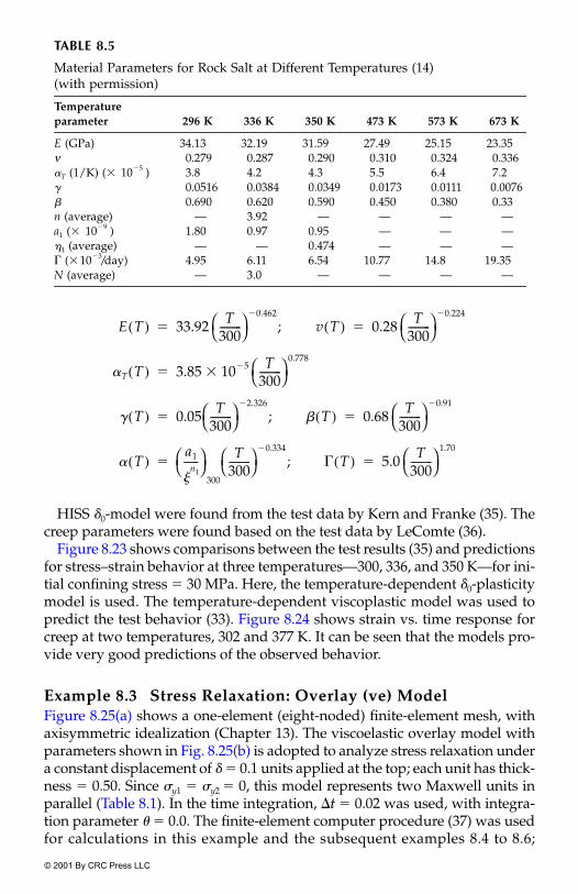
© 2001 By CRC Press LLC
HISS �0-model were found from the test data by Kern and Franke (35). Thecreep parameters were found based on the test data by LeComte (36).
Figure 8.23 shows comparisons between the test results (35) and predictionsfor stress–strain behavior at three temperatures—300, 336, and 350 K—for ini-tial confining stress � 30 MPa. Here, the temperature-dependent �0-plasticitymodel is used. The temperature-dependent viscoplastic model was used topredict the test behavior (33). Figure 8.24 shows strain vs. time response forcreep at two temperatures, 302 and 377 K. It can be seen that the models pro-vide very good predictions of the observed behavior.
Example 8.3 Stress Relaxation: Overlay (ve) ModelFigure 8.25(a) shows a one-element (eight-noded) finite-element mesh, withaxisymmetric idealization (Chapter 13). The viscoelastic overlay model withparameters shown in Fig. 8.25(b) is adopted to analyze stress relaxation undera constant displacement of � � 0.1 units applied at the top; each unit has thick-ness � 0.50. Since �y1 � �y2 � 0, this model represents two Maxwell units inparallel (Table 8.1). In the time integration, �t � 0.02 was used, with integra-tion parameter � � 0.0. The finite-element computer procedure (37) was usedfor calculations in this example and the subsequent examples 8.4 to 8.6;
TABLE 8.5
Material Parameters for Rock Salt at Different Temperatures (14) (with permission)
Temperature parameter 296 K 336 K 350 K 473 K 573 K 673 K
E (GPa) 34.13 32.19 31.59 27.49 25.15 23.35ν 0.279 0.287 0.290 0.310 0.324 0.336 T (1/K) (# ) 3.8 4.2 4.3 5.5 6.4 7.2� 0.0516 0.0384 0.0349 0.0173 0.0111 0.0076 � 0.690 0.620 0.590 0.450 0.380 0.33n (average) — 3.92 — — — —a1 (# ) 1.80 0.97 0.95 — — —�1 (average) — — 0.474 — — —� (# /day) 4.95 6.11 6.54 10.77 14.8 19.35 N (average) — 3.0 — — — —
10 5�
10 9�
10 3�
E T( ) 33.92 T300---------
0.462�
; v T( ) 0.28 T300---------
0.224�
� �
T T( ) 3.85 10 5� T300---------
0.778
#�
� T( ) 0.05 T300---------
2.326�
; � T( ) 0.68 T300---------
0.91�
� �
T( )a1
�n1
------
300
T300---------
0.334�
; � T( ) 5.0 T300---------
1.70
� �

© 2001 B
y CR
C P
ress LLC
FIGURE 8.23Comparisons between HISS �0-model predictions and test data at different temperatures (14).
© 2001 B
y CR
C P
ress LLC

© 2001 B
y CR
C P
ress LLC
FIGURE 8.24Comparisons between evp model and test data at different temperatures (14) (with permission).
© 2001 B
y CR
C P
ress LLC

© 2001 By CRC Press LLC
Sharma (38) provided assistance in these calculations. Figure 8.26 shows (axial)stress vs. time computed from the finite-element analysis. The results show thesame trends as the viscoelastic solution reported by Yamada and Iwata (39).
Example 8.4 Thermal Creep in Restrained Bar: evp ModelFigure 8.27(a) shows a five-element (eight-noded) mesh for a bar restrained ateach end. The bar is subjected to a temperature change �T � 10 degrees, whichvaries linearly up to time t � 0.1 and then is held constant [Fig. 8.27(b)]. Theparameters for the evp (Perzyna) model (Fig. 8.17) are as follows:
Time step �t � 0.02 was used with � � 0 in the integration.
FIGURE 8.25Stress relaxation: ve (Maxwell) model.
E 50 units, v 0.0� �
� 0.02, N 1.0� �
T 0.00096�
�y 0.0�
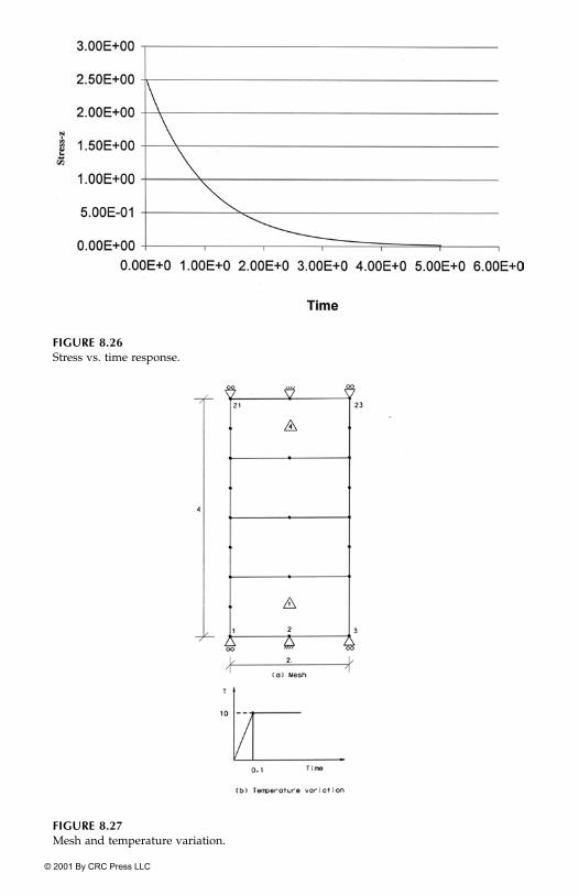
© 2001 By CRC Press LLC
FIGURE 8.26Stress vs. time response.
FIGURE 8.27Mesh and temperature variation.

© 2001 By CRC Press LLC
Figure 8.28 shows the computed axial stress vs. time curve. The stressincreases to a value of about 0.48, and thereafter it decreases with time. Thisresult is qualitatively similar to that reported by Yamada and Iwata (39) basedon an analytical solution and a finite-element procedure.
Example 8.5 Creep Analysis: ve, evp, and vevp Overlay Models with von Mises Plasticity CriterionFigure 8.29 shows a five-element mesh. The overlay model is used for ve, evp,and vevp versions (Table 8.1). A stress �0 � 800 units is applied at the top,kept constant up to four time units, and is then removed. In the time integra-tion, the time step �t � 0.10 is used with � � 0.0. The parameters used areshown in Table 8.6(a). Figure 8.30 shows computed strain vs. time plots forthe three models, which show consistent trends.
Example 8.6 Creep Analysis: ve, vp, and vevpModels with HISS PlasticityThe finite-element mesh used is the same as in Fig. 8.29. However, the loadapplied is �0 � 2000 units, and the parameters are different; they are shown inTable 8.6(b). Figure 8.31 shows computed strain vs. time plots for the threemodels. The trends in these plots are somewhat different than those in Fig. 8.30for the von Mises criterion because the HISS �0-model allows for continuousyielding.
The parameters chosen in Examples 8.3 to 8.6 are arbitrary, as the examplesare intended to show the capability of the models to simulate viscoelastic, vis-coplastic creep or both. The parameters of given materials should be found
FIGURE 8.28Stress vs. time behavior for restrained bar.

© 2001 By CRC Press LLC
from laboratory stress–strain–time responses under uniaxial, triaxial, and�orshear loadings.
Example 8.7 Viscoplastic Model for Asphalt ConcreteScarpas et al. (40) used the HISS �0-plasticity model (Chapter 7) with thePerzyna (evp) formulation for the characterization of the thermomechanicaland rate-dependent behavior of asphalt concrete.
Figures 8.32 to 8.34 show laboratory uniaxial compression, tension, andincremental creep test results, respectively, from testing with 100-mm highand 100-mm-diameter specimens of asphalt-concrete mix of type 0�16 with6% bitumen 80�100 (40). The tests were performed at different temperaturesand deformation rates ( ) for the compressive and tensile loadings. For thecreep behavior, the tests were performed at room temperature of 20$C. Thecreep response, Fig. 8.34(a), was divided in two parts; the first part up toabout 12 seconds, in which for each increment of stress, the strains stabilizesuch that � 0 [Fig. 8.34(b)], and the second part from 12 to 17 seconds, dur-ing which the strains increase at approximately the constant rate, Fig. 8.34(c).After about 17 seconds, tertiary creep occurred.
The HISS �0-plasticity model was used in the context of the evp model tocharacterize the first part of the creep response, in which, for a given stressincrement, the viscoplastic strains stabilized such that F � 0 (Fig. 8.3). For the
FIGURE 8.29Creep analysis: von Mises and HISS models.
�
�

© 2001 By CRC Press LLC
second part in which the creep strains do not stabilize, the behavior was sim-ulated by defining a creep initiation surface at the stress level when the firstpart stops. For subsequent stress (increments), the overstress, denoted by d inFig. 8.35, allows the use of the evp model, in which the creep strain increasesat a constant rate until the tertiary creep.
The hardening function, , was expressed by Scarpas et al. (40) as a functionof the dissipated energy, wp, during the first part of the creep response as
(7a)
where is the value of at 20$C up to which the response was considered tobe elastic. Plots of yield surfaces and of vs. wp are shown in Fig. 8.36(a) and(b), respectively. The latter is similar to expressed in terms of �vp, Eq. (8.4b).
For fracture and degradation analysis, Scarpas et al. (40) expressed fractureenergy given by the area under the stress (�) vs. w (crack opening length)(Fig. 8.37), which was expressed as
w � �c�cr (7b)
where �c is the characteristic length and �cr is the smeared crack strain. An alter-native and general approach based on critical disturbance can be used for micro-cracking leading to fracture and degradation (Chapter 12). Here disturbance, D,
TABLE 8.6
Parameters for ve, vp, and vevp Overlay: Von Mises and HISS Plasticity
(a) von Mises: �0 � 800
ve vp vevpUnit 1 Unit 2 Unit 1 Unit 2 Unit 1 Unit 2
Eν 0.20 0.20 0.20 0.20 0.20�
N 1.0 1.0 1.0 1.0 1.0�y 0.0 5000 750 0.0 1500F0 1.0 1.0 1.0 1.0 1.0
(b) HISS: �0 � 2000
ve vp vevpUnit 1 Unit 2 Unit 1 Unit 2 Unit 1 Unit 2
E 2 # 2 # 2 # 2 # 2 #ν 0.20 0.20 0.20 0.20 0.20�
N 1.0 1.0 1.0 1.0 1.0�y�F 10,000 0.0F0 1.0 1.0 1.0 1.0 1.0
�� � 0.06784, � � 0.755, n � 5.237, a1 � 0.46 # , �1 � 0.826, 3R � 50.
106 106 106 106 106
10 4� 10 4� 10 4� 10 4� 10 4�
106 106 106 106 106
10 4� 10 4� 10 4� 10 4� 10 4�
F� F� F�
10 10�
0ekwp�
�
0 0

© 2001 B
y CR
C P
ress LLC
FIGURE 8.30Predictions from overlay models: von Mises criterion.
© 2001 B
y CR
C P
ress LLC

© 2001 B
y CR
C P
ress LLC
FIGURE 8.31Predictions from overlay models: HISS �0-model.
© 2001 B
y CR
C P
ress LLC

© 2001 By CRC Press LLC
can be found from the test data (Figs. 8.32 and 8.33) by assuming linear elasticor elastoplastic (�0) model to characterize the RI behavior. The FA response canbe characterized by using the asymptotic stress (c) (Fig. 8.32). Then D can beexpressed as
(7c)
where Du, A, and Z are parameters dependent on temperature (T) and defor-mation rate
The parameters for the �0-plasticity and viscous response were determinedfrom the test data (Figs. 8.32 to 8.34) by using procedures described in thischapter and Chapter 7. They are listed below (40).
FIGURE 8.32Uniaxial compression tests for asphalt concrete (40).
D Du T , �( ) 1 eA T , �( )� vp
Z T ,�( )�
��
�( ).
� 0.089 at T 20$C�( ), � 0.442; n 2.1� � �
0 0.0865 at T 20$C�( ), k 2800� �
� 1.5 10 9� 1�sec; N# 0.32� �

© 2001 By CRC Press LLC
A thermoviscoplastic model was implemented in a three-dimensional,finite-element procedure (40), which was used to solve practical problemsinvolving pavement structures in which permanent deformations (rutting),and microcracking and fracture are important design considerations.
Example 8.8 Overlay Model: Closed-Form Solution (38) Consider two overlays 1 and 2 [Fig. 8.15(a)]. Let �0 be the applied (majorprincipal) stress, �1. Also, let the thickness of the two overlays t1 � t2 � 0.5,and , , and , be the major and minor principal stresses in overlays1 and 2, respectively.
The stresses (Eq. 8.49) in the overlays are
(8a)
FIGURE 8.33Uniaxial tension tests for asphalt concrete (40).
�11
�31
�12
�32
�1i ti� �1 or �1
1 12--- �1
2 12---� �1 or �1
1�1
2� 2�0� � �

© 2001 By CRC Press LLC
FIGURE 8.34Creep response for asphalt concrete (40).
FIGURE 8.35Secondary phase of creep due to overstress (40).

© 2001 By CRC Press LLC
and
(8b)
The strains in the overlays are
(8c)
and
FIGURE 8.36Hardening for asphalt concrete (40).
FIGURE 8.37Fracture energy for asphalt concrete at T � 25$C (40).
�3i ti� �3 or �3
1�3
2� 0� �
�11
�1e1
�1vp1 , �3
1�3e
1�3vp
1����
�12
�1e2
�1vp2 , �3
2�3e
2�3vp����

© 2001 By CRC Press LLC
However, � and � ; therefore,
(8d)
For axisymmetric idealization and the linear elastic model:
(8e)
and
where
Substitution of Eqs. (8c), (8d), and (8e) in Eq. (8a), and simplifications, lead to
(8f)
and
Equation (8f) can be used to solve for �1 and �3. Then from Eq. (8e), the expres-sions for stresses are found as
(8g)
�11
�12
�31
�32
�11
�12
�1 and �31
�32
� �3� � �
�11 a1�1e
1 2b1�3e1
��
�31 a1 b1�( )�3e
1 b1�1e1
��
�12 a2�1e
2 2b2�3e2
��
�32 a2 b2�( )�3e
2 b2�1e2
��
a1
E1 1 �1�( )1 �1�( ) 1 2�1�( )
--------------------------------------------- , b1
E1�1
1 �1�( ) 1 2�1�( )---------------------------------------------��
a2
E2 1 �2�( )1 �2�( ) 1 2�2�( )
--------------------------------------------- , b2
E2v2
1 �2�( ) 1 2�2�( )---------------------------------------------��
a1 a2�( )�1 2 b1 b2�( )�3� 2�0 a1�1vp1 2b1�3vp
1� ��
a2�1vp2 2b2�3vp
2� �
b1 b2�( )�1 a1 b1 a2 b2� � �( )�3� a1 b1�( )�3vp1 b1�1vp
1��
a2 b2�( )�3vp2 b2�3vp
2� �
�11 a1 �1 �1vp
1�( ) 2b1 �3 �3vp
1�( )��
�31 a1 b1�( ) �3 �3vp
1�( ) b1 �1 �1vp
1�( )��
�12 a2 �1 �1vp
2�( ) 2b2 �3 �3vp
2�( )��
�32 a2 b2�( ) �3 �3vp
2�( ) b2 �1 �1vp
1�( )��

© 2001 By CRC Press LLC
and the overall stresses in the overlay are
(8h)
Consider the yield function, F, in the Mohr–Coulomb criterion for the plasticresponse (Chapter 6)
(8ia)
Assume � � 0; then
(8ib)
Now for �1 and �2 � �3, the deviatoric stresses, , are given by
and
(8j)
Consider � � 30$ and cos � � hence
(8k)
The incremental viscoplastic strains are now evaluated as
(8l)
�1 �11t1 �1
2t2� �11
�12
�( )�2 �0� � �
�3 �31t1 �3
2t2� �31
�32
�( )�2 0� � �
FJ1
3---- � J2D �cos
� �sinsin3
--------------------------� c �cos��sin� 0� �
F J2D � c�cos 0� �
S˜
S12 �1 �3�( )
3--------------------------- , S2 S3
�1 �3�
3-------------------�� � �
J2D12--- S1
2 S22 S3
2� �( )
�1 �3�( )2
3--------------------------� �
3�2;
FJ2D----------- 3
4 J2D
--------------- ,J2D
�1----------- S1,
J2D
�3----------- S3� � �
F�1--------- F
J2D-----------
J2D
�1-----------�
12---� �
F�3--------- F
J2D-----------
J2D
�3-----------�
14---�� �
��1vp � F⟨ ⟩F�1--------- �t�
12---���1 �3�
2------------------- c��� �
��3vp � F⟨ ⟩F�3--------- �t�
14---� ��t��1 �3�
2------------------- c��� �

© 2001 By CRC Press LLC
The incremental viscoplastic strains in each overlay can be found by substi-tuting the respective values of the fluidity parameters (�1 and �1) and cohesion(c1 and c2) in Eq. (8l).
A computer routine was prepared for the foregoing closed-form solution[Sharma (38)]. It was used to obtain the closed-form solution with the followingparameters for a rock salt (7):
Applied stress, �0 � 160; time step, �t � 0.50; 1 bar � 100 KN� . The analysiscan be continued for various time levels; for example, for 60 days a total numberof increments � 121 are required. The finite-element computer procedure (37)was also used to solve the problem with the FE mesh [Fig. 8.38(b)]. Figure 8.39shows computed strain vs. time from the closed-form solutions and the com-puter procedure for three different confining pressures. Both correlate very welland yield essentially the same results.
Overlay 1 Overlay 2
Elastic modulus, E 4,700 15,400Poisson’s ratio, ν 0.24 0.24Fluidity parameter, � 2 # � bar�day 1 # �bar�dayCohesion, c 0.0 55.0 Thickness 0.50 0.50
FIGURE 8.38Finite-element mesh for rock salt problem: closed-form solution with overlay model.
10 4� 10 5�
m2

© 2001 By CRC Press LLC
Example 8.9 One-dimensional ElastoviscoplasticModel for CreepConsider the solution in Eq. 8.24. Figure 8.40(a)–(c) show plots of strain vs.time for H� � , , and psi with � � to . Here �0 � 30,000 psi,�y � 10,000 psi, and E � psi. It can be seen that as the value of � increases,the results approach the solution as per inviscid plasticity.
Example 8.10 One-dimensional Elastoviscoplastic Modelfor RelaxationDerive the relaxation solution for the one-dimensional case. Based on Eq.(8.2a), the viscoplastic rate is given by
(10a)
because the applied total strain is constant. The solution of Eq. (10a) is expressedas
(10b)
FIGURE 8.39Closed-form and computer results for strain vs. time behavior.
105 106 107 10 10� 10 2�
106
d�vp t( )dt
-----------------d�
e t( )dt
---------------�1E---d� t( )
dt--------------�� �
�vp t( )
� t( )dt
---------- C��

© 2001 By CRC Press LLC
For the case of stress relaxation, consider that a strain (increment) �0 isapplied at time t � 0. Stress at t � 0 is given by
�0 � E�0 (10c)
and since the viscoplastic strain is zero at t � 0, we have
(10d)
Therefore,
C � �0 (10e)
Consider the linear hardening response; hence,
(10f)
FIGURE 8.40Creep predictions for different values of H� and �.
� 0( )�E
----------------- C� 0�
� �y H��vp
��

© 2001 By CRC Press LLC
If the initial stress, �0, is greater than the yield stress (�y), stress relaxationwill occur and the overstress will tend to zero. For this case, the basic equationis given by Eq. (8.19), which, after substitution of �dt and from Eqs.(10a) and (10b) leads to
(10g)
The general solution for Eq. (10g) can be written as
(10h)
Using the initial condition for stress, is obtained as
(10i)
FIGURE 8.41Stress relaxation predictions for different values of H� and �.
d�vp
�vp
�E----d� t( )
dt-------------- 1
H��
-------� � t( )� �y H�� 0( )��
� t( ) Ce t H��E( )��� EH� E�------------------ �y H� 0( )�[ ]��
C
CE
H� E�------------------ E� 0( ) �y�[ ]�

© 2001 By CRC Press LLC
Therefore, the solution for stress is given by
(10j)
where � � 1��. As t → �,
which corresponds to the inviscid plasticity solution.Plots of � vs. strain for H� � , , and psi with � � to are
shown in Fig. 8.41. Here, �0 � 0.03, E � psi, and �y � 10,000 psi.
References
1. Perzyna, P., “Fundamental Problems in Viscoplasticity,” Adv. in Appl. Mech., 9,1966, 243–277.
2. Cormeau, I.C., “Viscoplasticity and Plasticity in Finite Element Method,” Ph.D.Dissertation, Univ. College at Swansea, U.K., 1976.
3. Zienkiewicz, O.C. and Cormeau, I.C., “Viscoplasticity-Plasticity and Creep inElastic Solids—A Unified Numerical Solution Approach,” Int. J. Num. Meth. inEng., 8, 1974, 821–845.
4. Katona, M.G. and Mulert, M.A., “A Viscoplastic Cap Model for Soils andRocks,” Chap. 17 in Mechanics of Engineering Materials, C.S. Desai and R.H.Gallagher (Editors), John Wiley, Chichester, U.K., 1984, 335–349.
5. Baladi, G.Y. and Rohani, B., “Development of an Elastic Viscoplastic Constitu-tive Relationship for Earth Materials,” Chap. 2 in Mechanics of EngineeringMaterials, C.S. Desai and R.H. Gallagher (Editors), John Wiley, Chichester, U.K.,1984, 23–43.
6. Kanchi, M.B., Zienkiewicz, O.C., and Owen, D.R.J., “The Viscoplastic Approachto Problems of Plasticity and Creep Involving Geometric Nonlinear Effects,”Int. J. Num. Methods in Eng., 12, 1978, 169–181.
7. Owen, D.R.J. and Hinton, E., Finite Elements in Plasticity: Theory and Practice,Pineridge Press, Swansea, U.K., 1980.
8. Desai, C.S. and Zhang, D., “Viscoplastic Model for Geologic Materials withGeneralized Flow Rule,” Int. J. Num. Analyt. Methods Geomech., 11, 1987,603–620.
9. Desai, C.S., Samtani, N.C., and Vulliet, L., “Constitutive Modelling and Anal-ysis of Creeping Slopes,” J. Geotech. Eng., ASCE, 121, 1995, 43–56.
10. Samtani, N.C., Desai, C.S., and Vulliet, L., “An Interface Model to DescribeViscoplastic Behavior,” Int. J. Num. Analyt. Methods Geomech., 20, 1996, 231–252.
11. Chia, J. and Desai, C.S., “Constitutive Modeling of Thermomechanical Re-sponse of Materials in Semiconductor Devices with Emphasis on InterfaceBehavior,” Report to NSF, Dept. of Civil Engng. and Engng. Mechs., Universityof Arizona, Tucson, AZ, 1994.
� t( ) EH� E�------------------ E� 0( ) �y�[ ]e t� H��E( )� E
H� E�------------------ �y H� 0( )�[ ]��
� t( ) EH� E�------------------ �y H� 0( )�[ ]→
105 106 107 10 5� 10 10�
106

© 2001 By CRC Press LLC
12. Desai, C.S., Chia, J., Kundu, T., and Prince, J., “Thermomechanical Responseof Materials and Interfaces in Electronic Packaging, Part I: Unified ConstitutiveModel and Calibration; Part II: Unified Constitutive Models, Validation andDesign,” J. of Electronic Packaging, ASME, 119, 1997, 294–309.
13. Basaran, C., Desai, C.S., and Kundu, T., “Thermomechanical Finite ElementAnalysis of Problems in Electronic Packaging Using the Disturbed StateConcept, Part I: Theory and Formulation; Part II: Verification and Applica-tion,” J. of Electronic Packaging, ASME, 120, March 1998.
14. Chia, J. and Desai, C.S., “Constitutive Modelling of Thermoviscoplastic Re-sponse of Rock Salt,” Proc. 8th Int Conf of Computer Meth. & Adv. in Geomech.,Balkema, Rotterdam, The Netherlands, 1994, 555–560.
15. Cristescu, N.D. and Hunsche, U., Time Effects in Rock Mechanics, John Wiley,Chichester, U.K., 1998.
16. Samtani, N.C. and Desai, C.S., “Constitutive Modeling and Finite ElementAnalysis of Slow Moving Landslides Using a Hierarchical Viscoplastic MaterialModel,” Report to NSF, Dept. of Civil Eng. and Eng. Mechs., University ofArizona, Tucson, AZ, 1991.
17. Hughes, T.J.R. and Taylor, R.L., “Unconditionally Stable Algorithms for Quasi-static Elasto-visco-plastic Finite Element Analysis,” Computers and Structures,8, 1978, 19–43.
18. Dinis, L.M.S. and Owen, D.R.J., “Elastic-viscoplastic Analysis of Plates by theFinite Element Method,” Computers and Structures, 8, 1978, 207–215.
19. Pan, T.Y., “Thermal Cyclic Induced Plastic Deformations in Solder Joints—PartI: Accumulated Deformations in Surface Mount Joints,” J. of Electronic Packaging,ASME, 113, 1991, 8–15.
20. Duwez, P., “On the Plasticity of Crystals,” Physical Reviews, 47, 6, 1935, 494–501.21. Zienkiewicz, O.C., Nayak, G.C., and Owen, D.R.J., “Composites and Overlay
Models in Numerical Analysis of Elasto-Plastic Continua,” Proc. Int. Symp. onFoundations of Plasticity, Warsaw, Poland, 1972.
22. Pande, G.N., Owen, D.R.J., and Zienkiewicz, O.C., “Overlay Models in Time-Dependent Nonlinear Material Analysis,” Computer and Structures, 7, 1977,435–443.
23. Hardy, H.R., Kim, R., Stefanko, R., and Wang, Y.J., “Creep and MicroseismicActivity in Geologic Materials,” Proc. 11th Symposium on Rock Mechanics (AIME),1970, 377–414.
24. Goodman, R.E., Introduction to Rock Mechanics, John Wiley & Sons, New York,1980, 196–201.
25. Coleman, D., “On Thermomechanics, Strain Impulses and Viscoelasticity,”Archives for Rational Mech. and Analysis, 17, 1964, 230–254.
26. Christensen, R.M., Theory of Viscoelasticity: An Introduction, Academic Press,London, 1982.
27. Schapery, R.A., “A Micromechanical Model for Nonlinear Viscoelastic Behaviorof Particle-Reinforced Rubber with Disturbed Damage,” Eng. Fracture Mech.,25, 1986, 845–867.
28. Schapery, R.A., “A Theory of Mechanical Behavior of Elastic Media with GrowingDamage and Other Changes in Structure,” J. Mech. Phys. Solids, 28, 1990, 215–253.
29. Valanis, K.C., “A Theory of Viscoplasticity Without a Yield Surface, Part I,”Archives of Mechanics, 23, 1971, 517–533.
30. Valanis, K.C., “An Endochromic Plasticity Theory for Concrete,” Mechanics ofMaterials, 5, 1986, 227–295.

© 2001 By CRC Press LLC
31. Krempl, E., “The Overstress Dependence of Inelastic Rate of DeformationInferred from Transient Tests,” Mat. Sc. Res. Int., 1, 1, 1995, 3–10.
32. Krempl, E. and Gleason, J.M., “Isotropic Viscoplasticity Theory Based on Over-stress (VBO): The Influence of the Direction of the Dynamic Recovery Theoremin the Growth Law of the Equilibrium Stress,” Int. J. of Plasticity, 12, 6, 1996,719–735.
33. Burke, P.M., “High Temperature Creep of Polycrystalline Sodium Chloride,”Doctoral Dissertation, Stanford Univ., Stanford, CA, USA, 1968.
34. Yang, J.M., “Thermophysical Properties: Physical Properties Data for RockSalt,” NBS 167, Nat. Bureau of Stand., Washington, DC, USA, 1981, 205–221.
35. Kern, H. and Franke, J.H., “The Effect of Temperature on the Chemical andMechanical Behavior of Carnallitic-Halite Rocks,” Proc. 1st Conf. Mech. Behaviorof Salt, Hardy, H. and Langer, M. (Editors), Pennsylvania State University, StateCollege, PA, 1981, 181–191.
36. LeComte, P., “Creep in Rock Salt,” J. Geophysical Research, 73, 1965, 469–484.37. Desai, C.S., “Computer Procedure DSC-SST2D and User’s Manuals,” Tucson,
AZ, 1999.38. Sharma, K.G., Private communication, 1998.39. Yamada, Y. and Iwata, K., “Finite Element Analysis of Thermo-Viscoelastic
Problems,” Seisan-Kenkyu, UDC 539.377, 24, 4, 1972, 41–46.40. Scarpas, A., Al-Khoury, R., Van Gurp, C.A.P.M., and Erkens, S.M.J.G., “Finite
Element Simulation of Damage Development in Asphalt Concrete Pavements,”Proc. 8th Int. Conf. on Asphalt Pavements, Univ. of Washington, Seattle, WA, USA,1997, 673–692.

© 2001 By CRC Press LLC
9The DSC for Saturated and Unsaturated Materials
CONTENTS9.1 Brief Review9.2 Fully Saturated Materials9.3 Equations9.4 Stress Equations
9.4.1 Modified Form of Terzaghi’s Equation9.5 Incremental DSC Equations9.6 Disturbance
9.6.1 Stress–Strain Behavior9.6.2 Volumetric or Void Ratio9.6.3 Effective Stress Parameter9.6.4 Residual Flow Concept
9.7 HISS and DSC Models9.7.1 Plasticity �0- and �1-Models
9.8 Softening, Degradation, and Collapse9.9 Material Parameters
9.9.1 Disturbance9.10 Examples
9.10.1 Back Predictions9.10.2 Saturated Soil: �1-Model9.10.3 Partially Saturated Soil: �1-Model9.10.4 DSC Model
Porous materials can involve full saturation when all the pores in their solidparticle matrix are filled with a fluid (or water). When the pores are only par-tially filled with the fluid, air or gas exists in the pore space not occupied bythe fluid. Testing and modelling of the behavior of saturated porous materi-als have advanced more than those for the partially saturated or unsaturatedmaterials. However, there has been a recent surge in research for the latterdue to their importance in such areas as geoenvironmental engineering, masstransport, and other engineering systems. In the following, we consider theDSC model for both.

© 2001 By CRC Press LLC
9.1 Brief Review
The literature on the modelling and mechanics of saturated and partially sat-urated porous materials is wide in scope. We do not intend to provide a com-prehensive review here; however, selected works are stated. A number ofearly works and textbooks (1–6) address these problems. Biot’s (7, 8) theoryof coupled mechanical response of porous saturated materials has provideda basis for a number of formulations and implementation in computer (finite-element) procedures (9–15); Chapter 13 considers the computer implementa-tion aspects. Terzaghi’s (1) one-dimensional idealization for the behavior ofsaturated soils can be shown to be a special case of Biot’s general three-dimensional formulation.
Although the research activity for the modelling of the behavior of par-tially saturated soils has increased recently, its importance for various engi-neering problems has been recognized for a long time. A number ofinvestigations have proposed analytical and empirical models for saturatedand expansive soils (16–33). Many recent works have considered the basicmechanisms of the behavior and have proposed analytical and numericalmodels, including the use of the critical-state, hierarchical single-surface(HISS) plasticity, disturbed state concept (DSC), coupled hydrothermo-mechanical aspects, and computer implementation (34–54).
In the context of fluid flow or seepage through porous media involvingboth saturated and unsaturated zones, Desai and co-workers (55–61) haveproposed and used the residual flow procedure (RFP). The RFP has proven(62) equivalent to the variational inequality methods (63, 64) and shown to bean alternative procedure for the fixed-domain analysis (65). Similar proce-dures have been used for free surface flow in (66, 67), and for computer(finite-element) analysis of unsaturated media (68, 69).
9.2 Fully Saturated Materials
Terzaghi (1) proposed the effective stress principle for defining the relationbetween stresses and fluid or pore water pressure in one-dimensional satu-rated media:
(9.1)
where is the total stress, is the effective stress carried by the solid skel-eton through particle contacts, and p is the pore water pressure. Here we shalluse uw to denote the pore water pressure instead of p because uw is commonlyused in the literature and because p is often used to denote the mean (effective)
�a
� p� � uw�� �
�a
�

© 2001 By CRC Press LLC
stress � The derivation of Eq. (9.1) is based on a number of assumptions,e.g., the stresses and pore water pressure are defined over a nominal area, A,and the contact area between solid particles, , is negligible during defor-mation. Thus, and uw do not allow for the changing (increasing) contactareas during deformation (Chapter 2).
If the DSC formulation (Chapter 2) is used, the equilibrium of forces lead to
(9.2)
where D is disturbance, is the fluid stress, which can be different from p inEq. (9.1), and is the stress at contacts. Equation (9.2) allows for the calcu-lation of and as functions of D, which is expressed in terms of contactarea, (or void ratio, e); details are given in Chapter 2.
The theory developed by Biot (7, 8) is often used for the analysis of the cou-pled behavior of saturated media. It is also modified to characterize unsatu-rated media by introducing correction or residual (RFP) terms to allow for thepartial saturation. We shall give details of Biot’s equations and computerimplementation in Chapter 13. Constitutive models for saturated and par-tially saturated media, and the equations that can be used for implementa-tion in solution procedures, are discussed in this chapter. We define thequantities based on nominal area, as in Terzaghi’s theory.
9.3 Equations
A symbolic representation of an element of partially saturated material isshown in Fig. 9.1. The responses are decomposed here into those of the solidskeleton, fluid (water), and gas (air). If the material is dry, the total force, is in equilibrium with the force, , in the solid skeleton:
(9.3)
If the material is fully saturated, the force equilibrium gives
(9.4a)
and
(9.4b)
J1
3---- .
As
�
�a 1 D�( )p f D�
s��
p f
�s
�s p f
As
Fa,F
Fa F Fi
Fc
�� �
Fa F uw( ) Fw�( )��
�a
� uw( ) uw �( )��

© 2001 By CRC Press LLC
where uw and are the pore water pressure and effective stress in the solidskeleton, respectively. It is evident here that the responses of the solid skele-ton and pore water are coupled; hence, and uw are affected by each other.
For partially saturated materials, the equilibrium can be expressed as
(9.5a)
or
(9.5b)
(9.5c)
where ug is the pore gas or air pressure and s � ug � uw is the matrix suction;if the gas happens to be air, s � ua � uw, where ua is the pore air pressure.
FIGURE 9.1Dry and saturated materials.
�
�
Fa F uw, ug( ) Fw�, ug( ) Fg
�, uw( )� ��
Fa F s( ) Fw�, s( ) Fg
�, s( )���
�a
� s( ) uw �, s( ) ug �, s( )���

© 2001 By CRC Press LLC
Again, Eq. (9.5) indicates that the responses of the solid skeleton, pore water,and pore air are coupled.
In general, it would be necessary to define the constitutive equations forthe solid skeleton and water and air phases from appropriate laboratorytests. Then, in a general solution (finite-element) procedure, coupled formu-lations involving displacements, pore water pressure, and pore air pressureare independent variables; in that case, all three will be evaluated duringincremental procedures. However, it may become difficult to formulate sucha coupled problem, particularly the constitutive equations for the threephases. Thus, approximate procedures can be developed. In a simple approx-imation, the response is considered to be uncoupled, in which the values ofuw and ug are known and can be converted into equivalent “loads,” as in theRFP.
In a somewhat more rigorous procedure, the stresses computed from dis-placements based on effective response can be used to evaluate relations thatdefine uw and�or ug, which can then be used for the next step of incrementalanalysis for the effective response. Here the computed values of uw and�or ug
can be converted into equivalent or residual vectors that are integrated in thecoupled equations, e.g., based on Biot’s theory (see Chapter 13).
9.4 Stress Equations
For the case of a partially saturated medium with air and water in the pores,the total stress tensor, , can be expressed, based on Eq. (9.5), as
(9.6a)
(9.6b)
where is the effective stress tensor, and f(s) is the function of air and porewater pressures. Figure 9.2 shows plots of expanding yield surfaces accord-ing to the HISS plasticity model (Chapter 7); the slope of the ultimate enve-lope (�) can increase with suction. Here, the intercept on the J1-axis can bederived from Eq. (9.6) as
(9.7a)
or
(9.7b)
�ija
�ija
�ij ua�ij f ua uw�( )�ij���
�ij ua f s( )�[ ]�ij��
�ij
�iia
�ii 3ua 3 f s( )���
J1a J 1 3ua 3 f s( )���

© 2001 By CRC Press LLC
or
(9.7c)
where and are the first invariants of the total and effective stress tensors,respectively, and and are the total and effective mean pressures, respec-tively. The existence of suction modifies the response of the material andincreases the magnitude of the material’s tensile strength, which is propor-tional to the term 3f(s) and is called the bonding stress. If the material is fullysaturated, Eq. (9.7) reduces to
(9.8a)
or
(9.8b)
as in Terzaghi’s effective stress equation.
9.4.1 Modified Form of Terzaghi’s Equation
A simplified form of Eq. (9.7), as a modification of Terzaghi’s one-dimensionaleffective stress equation for saturated materials, was proposed by Bishop (17)for partially saturated soils:
(9.9)
FIGURE 9.2Expanding yield surfaces.
pa p ua f s( )���
J1a J1
pa p
J1a J1� 3uw�
pa p� uw�
�a
� ua � ua uw�( )���

© 2001 By CRC Press LLC
where � is often called the weighting or effective stress parameter. In termsof effective stress , Eq. (9.9) is written as
(9.10)
which, in terms of mean effective pressure, � becomes
(9.11a)
(9.11b)
where is the total mean stress � is the total mean stress in excess ofair pressure (ua), which is often referred to as net mean stress, and s is thematrix suction or suction � ua � uw .
The parameter � attains a value of unity for saturated materials when therelative saturation Sr � 1. Then Eq. (9.10) reduces to Eq. (9.1). For dry materi-als, � � 0 and ua � 0; hence, Eq. (9.10) reduces to indicating that thetotal or observed stress equals the effective or solid stress.
A plot of � vs. for different soils is shown in Fig. 9.3; the curves wereadopted from different publications, which are detailed in (20). The validity ofEq. (9.10) has been questioned by some investigators (20, 22, 23) on the groundthat the parameter � may not be defined based only on an index property suchas Sr , particularly when the material can experience plastic deformations,microcracking leading to softening (degradation) and collapse. Hence, we
FIGURE 9.3Relations between � and Sr (20, which gives details of the origins of curves). Reproducedfrom Geotechnique, Institute of Civil Engineers, London, England.
�
� �a ua�( )� � ua uw�( )�
p J 1�3,
p pa ua�( ) � s( )��
p pa� � s( )�
paJ 1�3, pa
� �a,�
Sr

© 2001 By CRC Press LLC
propose the following generalization based on Eq. (9.6) as
(9.12)
where D is the disturbance as a function of plastic strain trajectory (), voidratio (e), or plastic work (w) (Chapter 3). If D is expressed as a function of Sr
or s, and since the effective stress, , is dependent on Sr or s, Eq. (9.12) canbe written as
(9.13)
Figure 9.4 shows a schematic of D vs. or e, as functions of suction or satu-ration. Various definitions of D are given later.
9.5 Incremental DSC Equations
The microstructure (solid skeleton or matrix) experiences relative particlemotions as affected by irreversible strains, air and the pore water pressures,and suction. Hence, the disturbance can be considered to occur in the solidskeleton and can be incorporated through the effective stress. Then for thesaturated case, the observed effective stress, (in the solid skeleton), can beexpressed as
(9.14a)
FIGURE 9.4Disturbance vs. plastic strain trajectory ( ) or void ratio (e).
� �a ua�( ) f Sr, s, D( ) ua uw�( )��
�
� s( ) �a s( ) ua D , e, w, s( ) ua uw�( )���
�a
�ija 1 D�( )�ij
i� D�ij
c�

© 2001 By CRC Press LLC
or
(9.14b)
where , , and are the vectors of stresses in the observed, relativeintact, and fully adjusted states in the solid skeleton (Fig. 9.5), respectively,and D is the disturbance in the solid skeleton, which can be defined in differ-ent ways (to be covered later). The incremental form of Eq. (9.14) can bewritten as
(9.15a)
or
(9.15b)
where and are the constitutive matrices for the responses of the RI andFA parts of the solid skeleton, respectively; and are the strains in the RIand FA parts, respectively; and dD is the increment or rate of D.
In the case of partially saturated materials, Eq. (9.15) can be written as afunction of s (or Sr) as
(9.16)
Thus, the RI and FA responses, and D, are expressed as functions of suction(s) or the saturation ratio (Sr).
Equation (9.15) or (9.16) can be integrated to obtain the effective response.Then the pore water and air pressure or suction can be evaluated using theeffective quantities if the total stress is known. This is usually possible in lab-oratory tests where both the total and effective response and suction are mea-sured. For example, in the case of saturated materials [Eq. (9.8)], the pore
FIGURE 9.5Mixture, and RI and FA parts in solids.
�˜
a 1 D�( )�˜
i� D�
˜c
�
�˜
a�˜
i�˜
c
d�˜
a 1 D�( )d�˜
i Dd�˜
c dD �˜
c�˜
i�( )� ��
d�˜
a 1 D�( )C˜
id
i
˜DC
˜cd
c
˜� dD �
˜c
�˜
i�( )��
C˜
iC˜
c
i
˜
c
˜
d�˜
a 1 D s( )�[ ]C˜
is( )d
i
˜D s( )C
˜c
s( )dc
˜dD s( ) �
˜c
�˜
i�( )� ��

© 2001 By CRC Press LLC
water pressure can be evaluated as
(9.17)
where J1 (� �1 � �2 � �3) is the first invariant of the total stress tensor, �ij,measured in the laboratory, and is the effective invariant computed fromthe integration of Eq. (9.15). Examples of prediction of laboratory behaviorusing Eq. (9.15) are given later in section 9.10.
In the case of partially saturated tests, the air pressure, ua, can be computedfrom [Eq. (9.7)]
(9.18)
where D is the disturbance (Fig. 9.4) and s � ua � uw is the value of suction inthe test.
In the case of general boundary-value problems, when coupled (e.g., Biot’s)equations are solved incrementally, say, by using a finite-element procedure(Chapter 13), the values of uw and ua are computed as independent variablestogether with the displacements. Alternatively, a separate relation for ua maybe postulated; then the coupled formulation can involve only the displace-ments and pore water pressures, uw .
9.6 Disturbance
Disturbance can be evaluated using laboratory test data such as stress–strain,volumetric (void ratio), effective (pore water pressure), or nondestructiveproperties. Then it can be expressed as
(9.19a)
or
(9.19b)
where s and are the suction and initial effective mean pressure, respectively,for a given test, and D and w are the (deviatoric) plastic strain trajectory and
uw
J1a J1�
3---------------- pa p�� �
J1
J1 J1a 3ua�( ) f D( ) ua uw�( )��
D s, p0( ) Du1 s, p0( ) 1 e�A1 s , p0( )D�
Z1 s , p0( )
�
D s, p0( ) Du2 s, p0( ) 1 e�A2 s , p0( )w
Z1 s , p0( )�
�
p0

© 2001 By CRC Press LLC
plastic work, respectively. A number of possible ways to define the distur-bance are described ahead. Although the disturbances from different mea-sured quantities characterize the same phenomenon, their magnitudes andvariations may not be the same. Hence, when used in the stress [Eq. (9.16)], Dneeds to be determined from appropriate correlations with respect to distur-bances from different definitions.
9.6.1 Stress-Strain Behavior
Two of the possible ways for defining the disturbance with respect to thestress–strain response are indicated in Fig. 9.6. Figure 9.7 (a to f) shows thestress–strain volume change behavior of a partially saturated soil as reportedby Cui and Delage (46) from triaxial tests under different confining pressures(�3) and suction (s). The test data show that under some combinations of �3
FIGURE 9.6Definitions of disturbance.

© 2001 By CRC Press LLC
FIGURE 9.7(a)Observed stress–strain responses with different confining pressures and suction (46).

© 2001 By CRC Press LLC
FIGURE 9.7(b)(continued)

© 2001 By CRC Press LLC
FIGURE 9.7(c)(continued)

© 2001 By CRC Press LLC
FIGURE 9.7(d)(continued)
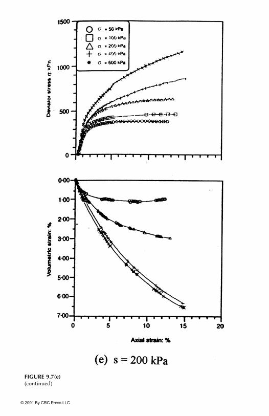
© 2001 By CRC Press LLC
FIGURE 9.7(e)(continued)

© 2001 By CRC Press LLC
FIGURE 9.7(f)(continued)

© 2001 By CRC Press LLC
and s, softening and dilative response are exhibited, while for other combina-tions, the response is mainly hardening and compactive.
The procedures for disturbance used for dense and loose soils (Chapter 3)can be used for partially saturated soils for test data at a given value of thesuction. For the softening response, the RI behavior can be simulated as thehardening response (nonlinear elastic or elastoplastic) as the continuation ofthe prepeak curve. For the hardening behavior [Fig. 9.6(b)], the RI responsecan be characterized based on the response under constant volume or den-sity, iv . As a simplification, the zero stress (i�) can be adopted as the RIresponse. In both cases, the FA response (c) can be characterized based on thecritical-state condition (c).
The choice of the RI and FA responses can depend on the behavior of agiven material. For instance, the FA state can be defined based on theresponse at full saturation (i.e., zero suction), and the RI state on the responseat (approximately) zero saturation (i.e., high value of suction).
Alternatively, the response under the zero suction (saturated) conditioncan be adopted as RI [Fig. 9.6(c) and (d)]. The FA response can be character-ized as the critical-state behavior.
The disturbance function, D, can be expressed as
(9.20)
or
(9.21)
In the case of Fig. 9.6(a) and (b), the disturbance will vary from 0 to 1. Itsvalue can increase from zero to greater than unity, and then decrease forFig. 9.6(c), whereas from Fig. 9.6(d), it will vary from 0 to 1.
In the first alternative, softening will occur with positive D [Fig. 9.6(a)],while stiffening will occur with negative D [Fig. 9.6(b)]. Hence, it will be nec-essary to adopt appropriate values of quantities to identify softening andstiffening. For instance, with respect to the initial void ratio, e � will indi-cate stiffening, and for e � , softening will occur. In the case of the secondalternative, stiffening will occur with respect to the RI response at s � 0. Thus,disturbance with positive or negative sign will need to be used in Eq. (9.15).
9.6.2 Volumetric or Void Ratio
Disturbance can also be expressed in terms of the void ratio (e) or specific vol-ume as
(9.22)
D�
i�
a�
�i
�c
�------------------�
D
i
a�
i
c
�----------------�
ec
ec
Dg
emax ea�
emax emin�
--------------------------�

© 2001 By CRC Press LLC
where Dg denotes the “global” disturbance, and are the maximumand minimum void ratios, respectively, and is the observed void ratio.Figure 9.8 shows a schematic plot of e vs. stress (e.g., mean net stress). Thevalue of Dg varies from zero to unity. However, in practice, a porous materialmay have an initial void ratio before testing, and for a given load-ing, it may tend toward the final void ratio, . In that case, the disturbancefor the range of loading will start with an initial value of D0 (� 0) correspond-ing to e0 and will tend toward the final disturbance, Df or Du (� 1); thus, thedisturbance will vary between D0 and Df (Fig. 9.8). If necessary and appropri-ate, the local disturbance, D�, for the given load can then be expressed as
(9.23)
which will vary from zero to unity for the given loading. It may be noted thatthe definition of Dg [Eq. (9.22)] can be expressed as
(9.24)
in which Dg depends on factors such as plastic strains and suction. Thus, Dg
can be found from measurements of Sr during laboratory tests under differ-ent values of and s. A physical interpretation of Eq. (9.24) is that degree ofsaturation can be considered a measure of disturbance.
FIGURE 9.8Schematic of void ratio (e) vs. stess.
emax emin
ea
e0�emax( )
e f
D�e0 ea
�
e0 e f�
-----------------�
Dg 1 Sr��
p0

© 2001 By CRC Press LLC
9.6.3 Effective Stress Parameter
The foregoing definition of disturbance, which is applicable for the entirestress–strain behavior, can be considered analogous to the representation ofthe behavior of partially saturated material in terms of peak (failure) strengthproposed by Khalili and Khabhaz (33). Here the shear strength, , isexpressed as
(9.25)
where c� is the effective cohesion, �� is the effective angle of friction, and �is the total stress. The drained shear strength of soil at full saturation, 0, iswritten as
(9.26)
where, at saturation, ua � uw . The difference between and 0 can be consid-ered as the contribution to the strength due to suction; therefore,
(9.27)
and
(9.28)
Figure 9.10 shows plots of shear strength vs. matric suction, s, reported byGan et al. (70) at different initial void ratios. The disturbance at (peak)
FIGURE 9.9Disturbance vs. void ratio (e) between test range of e (e0 to ef).
c� � ua�( ) � ua uw�( )�[ ] ��tan��
0 c� � ua�( ) ��tan��
0� � ua uw�( ) ��tan�
� 0�
ua uw�( ) ��tan----------------------------------------�

© 2001 By CRC Press LLC
strength, Dp, can now be expressed using Eq. (9.27) as
(9.29a)
(9.29b)
Figure 9.3 shows the variation of Sr with � for different soils as reported in(20). Thus, for full saturation, Sr � 1 and � � 1; hence, Dp � 0. For dry condi-tion, Sr � 0 and � � 0; therefore, Dp � 1. Thus, Dp, as plotted schematically inFig. 9.11, shows that it varies from 0 to 1 as saturation varies from 1 to 0, i.e.,from a fully saturated to a dry condition.
In Eq. (9.29), the parameter � represents the change (increase) in strengthfrom that in the fully saturated (RI) state to that in the partially saturatedstate. Thus, the parameter � can be treated as a measure of the disturbance.For the entire stress–strain response, it will depend on factors such as plasticstrain or work, initial pressure, and suction.
9.6.4 Residual Flow Concept
The idea of disturbance can be derived from the residual flow procedure (RFP)proposed by Desai and co-workers (55–61) for free surface seepage in two-and three-dimensional problems. Its application for uncoupled seepage andstress analysis is given by Li and Desai (58). In the RFP, a residual or correctionfluid “load” is evaluated based on the difference between permeabilities or
FIGURE 9.10Shear strength vs. matric suction (70).
Dp
ua uw�( ) �� 0�( )�tanua uw�( ) ��tan
--------------------------------------------------------------------�
1 ���

© 2001 By CRC Press LLC
conductivities or the degree of saturation, in the saturated and unsaturatedconditions. The RFP concept can also be used to modify the coupled equa-tions for saturated media, say, in Biot’s theory, so as to allow for partialsaturation.
Figure 9.12(a) shows a porous (soil) medium in which the material is satu-rated below the free surface (FS) and partially saturated above the FS. Thefluid pressure (uw) is positive in the saturated zone and negative (suction) inthe partially saturated zone. Figure 9.12(b) and (c) show variations of thecoefficient of permeability (k) and saturation with pressure, respectively. Inthe fully saturated state, the permeability is ks, while Sr � 1.0. In the partiallysaturated regions, the permeability is kus � ks and saturation Sr � 1. As thesuction increases, the permeability and saturation decrease and approachasymptotically those in the dry state.
The disturbance, D, can be expressed as
(9.30)
and
(9.31)
Initially, in the saturated or RI state, kus � and Sr � 1; finally, kus � kf andSr � Srf. Hence, D varies from 0 to 1. Thus, if the values of permeabilities or
FIGURE 9.11Plot of Dp vs. Sr .
Dk
ks kus�
ks k f�-------------------�
Ds
1 Sr�
1 Srf�-----------------�
ks

© 2001 By CRC Press LLC
saturation are measured during deformation of a specimen, the values of Dcan be evaluated.
It is possible that the values and variations of D, according to the foregoingdefinitions, are not the same as those required in the constitutive equations[Eq. (9.16)]. Hence, it will be necessary to establish appropriate correlationsbetween disturbances from different methods in order to define the Drequired in the DSC equations based on stresses [Eq. (9.16)].
9.7 HISS and DSC Models
The DSC and its hierarchical versions, e.g., HISS �0- and �1-plasticity models(Chapter 7), can be used to develop constitutive equations for saturated andpartially saturated materials. A number of approximate and general formu-lations are possible. We describe some of them here for partially saturated
FIGURE 9.12Residual flow procedure.

© 2001 By CRC Press LLC
materials. Models for saturated materials can be derived as special cases ofthose for the partially saturated case.
9.7.1 Plasticity �0- and �1-Models
If the effective response of the porous material (e.g., soil) is essentially theplastic yielding or hardening type [Fig. 9.7 (c, d, e)], the �0- and �1-versions inthe HISS plasticity approach can be used by expressing the parameters asfunctions of suction (s) or degree of saturation, Sr .
The yield function, F, for the �0-model (Chapter 7) can now be written as
(9.32)
where the parameters are expressed in terms of suction, s. Here the effectivestress quantities are nondimensionalized with respect to pa; however, theoverbar [as in Eq. (7.1)] is not shown, in order to avoid confusion with effec-tive quantities.
If the behavior exhibits nonassociative properties, �(s) in Eq. (9.32) can beexpressed as
(9.33)
where � is the nonassociative parameter, �0 is the value of � at the end of ini-tial (hydrostatic) loading, and rv is the ratio of the volumetric plastic strainsto the total plastic strain trajectory [Eq. (7.5), Chapter 7].
Figure 9.13 shows a schematic of F [Eq. (9.32)] in which the intercept 3Rdenotes the bonding (tensile) strength of the material given by
(9.34)
FIGURE 9.13Schematic of yield surfaces and bonding strength.
F J2D � s( )J1n s( )
� s( ) J1( )2��[ ] 1 � s( )Sr�[ ] 0.5�
� 0� �
�Q s( ) � � s( ) �0 ��( ) 1 rv�( )��
J1a J1 3R s( )��

© 2001 By CRC Press LLC
The bonding strength will increase with suction, and the yield surface willmove to the left as suction increases, starting with zero suction (Sr � 1). Theparameters’ dependence on suction needs to be defined on the basis of labo-ratory tests; an example is given subsequently.
The incremental effective stress equations [Eq. (9.16)] can be used to repre-sent the behavior of partially saturated materials by using the elasticity andplasticity parameters.
A number of investigators have proposed and used elastic, thermoelastic,and elastoplastic models for partially saturated soils (37–41, 43–46, 48–53).The elastoplastic models based on the critical-state concept have been usedcommonly (41, 43, 45, 46, 50–52). The HISS and DSC models have been usedrecently (47, 54). The HISS model has been shown to include the critical-stateand other plasticity (hardening) models as special cases (see also Chapter 7).
9.8 Softening, Degradation, and Collapse
Under certain combinations of suction (s) and initial (cell) pressure, , anddensity (�0), a material may exhibit softening or degradation behavior[Fig. 9.7(a, b, f)]. As discussed in Chapter 10, the microstructural adjustmentmay entail threshold transition states, some of which lead to instability or col-lapse of the microstructure. The latter is identified by the critical value of dis-turbance, Dc, indicated in Fig. 9.4. Thus, the idea of critical disturbance canprovide a means for the evaluation of instability or collapse in dry, satu-rated, or partially saturated materials; this is discussed in Chapter 13 andAppendix I.
The incremental constitutive equations [Eq. (9.16)] can be used to allow forthe disturbance, which provides for the simulation of softening and collapseresponses. Note that the general Eq. (9.16) includes plastic hardeningresponse as a special case, when D � 0.
9.9 Material Parameters
The procedures for finding the parameters in the DSC/HISS models fromlaboratory tests are presented in Chapters 3 and 7. Here we briefly describetheir evaluation for partially saturated soils.
Elastic. The modulus such as E and � or G and K are found as averageslopes of unloading curves and can be expressed as functions of suction, asnecessary.
Ultimate Parameters. The parameters associated with the ultimate asymp-totic stress–strain response are �, �, and R. They are determined from test
p0

© 2001 By CRC Press LLC
data for given saturation (Sr) or suction (s) and then expressed as
(9.35a)
(9.35b)
(9.35c)
Here � represents the slope of the ultimate envelope in –J1 space(Fig. 9.13), and � is related to the shape of F in �1–�2–�3 space (Chapter 7).The bonding strength R can be found approximately from
(9.35d)
where is the (cohesion) intercept along the -axis, when J1 � 0(Fig. 9.13) and is based on the assumption that the ultimate envelope is lin-ear. If it is nonlinear, the slope to the initial part of the envelope can be usedto define .
Hardening Parameter. The hardening or growth function, �, in Eq. 9.32can be expressed as
(9.36)
where a1 and �1 are the hardening parameters dependent on suction, and isthe trajectory of plastic strains.
Phase Change Parameter. This parameter is associated with the state ofvolume change when transition from compaction to dilation occurs and thechange in volumetric strains, dv, vanishes (Fig. 9.7). It can be expressed as afunction of suction as
(9.37)
For the FA response, the parameters can be defined on the basis of the con-strained liquid or constrained liquid–solid assumption (Chapter 7). For theformer, only the bulk or hydrostatic response is relevant, and if the behavioris represented by using the bulk modulus, K, it can be expressed as a functionof suction as
(9.38)
� � s( )�
� � s( )�
R R s( )�
�( ) J2D
3R s( )ca s( )� s( )
---------------�
ca J2D
�
� s( )a1 s( )
�1 s( )------------�
n n s( )�
K K s( )�

© 2001 By CRC Press LLC
For the liquid–solid assumption, the critical-state concept can be used.Here the critical responses can be expressed using the following equations(Chapter 4):
(9.39a)
and
(9.39b)
where the slopes and � are both expressed as functions of suction.
9.9.1 Disturbance
For a set of tests under given suction, s, Eq. (9.19a) can be written as
(9.40)
Plots of ln D and lead to the values of A and Z (Chapter 3). Du isobtained based on ultimate or residual values (of stress) (Fig. 9.6); its valuecan also often be adopted as 1 or close to 1 (� 0.95). Then A, Z, and Du can beexpressed as
(9.41a)
(9.41b)
(9.41c)
9.10 Examples
We now consider examples of application of the HISS and DSC models for thebehavior of saturated and partially saturated materials. Two examples of theuse of the HISS plasticity models for saturated clay and sand are presented asExamples 7.7 and 7.8 in Chapter 7. Additional examples are given here.
J2Dc m s( )J1
c�
ec e0c
� s( )ln J1c
3pa--------
��
m
ln A Z ln D( )� ln ln Du D�
Du-------------------
� D�
� �
D�
A A s( )�
Z Z s( )�
Du Du s( )�

© 2001 By CRC Press LLC
Example 9.1 Saturated SandA series of laboratory undrained cyclic (frequency � 0.10 Hz) to multiaxialtests were performed on saturated Ottawa sand with cubic specimens (10 �10 � 10 cm) under different initial confining pressures � �3 � 69, 138,and 207 kPa and at relative density Dr � 60%. Figures 9.14 to 9.16 show testdata in terms of applied cyclic stress, �1 � �3 � �d vs. time, axial strain (1) vs.time, pore water pressure uw vs. time, and shear stress (�d) vs. axial strain (1)for the three values of , respectively (71–73). These data were used to findthe parameters. The (average) values of parameters obtained using the pro-cedures in Chapters 3 and 7 are shown in Table 9.1; brief details are givenbelow (74).
Elastic Moduli. Figure 9.17 shows typical data in terms of oct vs. 1 and2 � 3 from quasi-static or one-way (loading, unloading, reloading) CTC(�1 � �2 � �3) tests, for � 207 kPa. The values of E and � were found from
(1a)
(1b)
where Ei (i � 1, 2, 3) are the slopes shown in Fig. 9.17.Ultimate. Figure 9.18 shows a schematic in terms of J1 vs. in which the
ultimate and critical-state or phase change envelopes are shown. The ultimateparameters, � and �, were found using the procedure given in Chapter 7.
TABLE 9.1
Material Parameters for the DSC Model: Ottawa Sand (72, 73)
Parameter Value
Elastic E 193,000 kPa� 0.380
Ultimate� 0.123� 0.00
Phase Change n 2.45Hardening h1 0.845
h2 0.0215FA (Critical state) 0.150
� 0.0200.601
Disturbance � 4.22Z 0.43Du 0.99
m
e0c
�0
�0
�0
E 32
-------E1�
�2�1
E2 E3�-------------------�
J2D
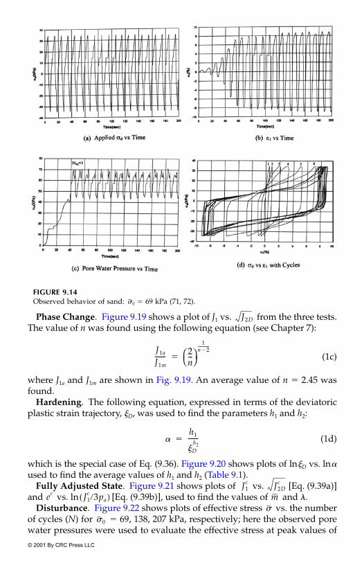
© 2001 By CRC Press LLC
Phase Change. Figure 9.19 shows a plot of J1 vs. from the three tests.The value of n was found using the following equation (see Chapter 7):
(1c)
where J1a and J1m are shown in Fig. 9.19. An average value of n � 2.45 wasfound.
Hardening. The following equation, expressed in terms of the deviatoricplastic strain trajectory, D, was used to find the parameters h1 and h2:
(1d)
which is the special case of Eq. (9.36). Figure 9.20 shows plots of lnD vs. ln�used to find the average values of h1 and h2 (Table 9.1).
Fully Adjusted State. Figure 9.21 shows plots of vs. [Eq. (9.39a)]and vs. ln [Eq. (9.39b)], used to find the values of and �.
Disturbance. Figure 9.22 shows plots of effective stress vs. the numberof cycles (N) for � 69, 138, 207 kPa, respectively; here the observed porewater pressures were used to evaluate the effective stress at peak values of
FIGURE 9.14Observed behavior of sand: � 69 kPa (71, 72).�0
J2D
J1a
J1m------- 2
n---
1
n�2------------
�
�h1
Dh2
-------�
J1c J2D
c
ec J1c�3pa( ) m
��0

© 2001 By CRC Press LLC
cyclic stress (Figs. 9.14 to 9.16). Note that the ultimate asymptotic value of theeffective stress is zero; hence, Du � 0.99 was used. The disturbance was foundusing the following equation:
(1e)
where is the RI effective stress computed using the �0-model to simulatethe first cycle response without cyclic degradation (73). The disturbance func-tion was expressed as
(1f)
Equations (1e) and (1f) were used to obtain plots of ln(D) vs. ln[�ln(1 �)]as shown in Fig. 9.23, which provided the values of A and Z. Plots of
disturbance vs. D(N) are shown in Fig. 9.24. Here, the test data values referto Eq. (1e), while the function values refer to Eq. (1f) in which the parametersA, Z, and Du (Table 9.1) were used.
FIGURE 9.15Observed behavior of sand: � 138 kPa (71, 72).�
D�
i�
a�
�i
�c
�------------------�
�i
D Du 1 eAD
Z�
�( )�
D0.99----------

© 2001 By CRC Press LLC
9.10.1 Back Predictions
The dynamic finite-element procedure (74–76 and Chapter 13) was used topredict the behavior of the test specimens. Figure 9.25 shows the finite-ele-ment mesh and loading with frequency � 0.1 Hz. The latter involved applyingthe confining stress incrementally and then applying the cyclic, �d, stressincrementally with different amplitudes (Figs. 9.14 to 9.16), as it was done inthe laboratory tests.
Figures 9.26 to 9.28 show comparisons between predicted and observedeffective stress and excess pore water pressure vs. time (or number ofcycles) for � 69, 138, and 207 kPa, respectively. The pore water pressureswere computed using Eq. (9.17).
In the above-mentioned back predictions, the parameters used were thosefor the tests used to find them, the relative density of which was Dr � 60%. Inorder to validate the model further, the average parameters (Table 9.1) wereused to predict an independent test, and not used to find the parameters. Thistest involved � 69 kPa and relative density Dr � 40%. Figure 9.29 showscomparisons between predictions and test data in terms of the effective stress
FIGURE 9.16Observed behavior of sand: � 207 kPa (71, 72).�
�( )�0
�0

© 2001 By CRC Press LLC
and excess pore water pressure (uw). The model also provides good pre-dictions for the independent tests (74).
Liquefaction. The DSC provides a basis for the evaluation of instabilityand liquefaction. Analysis and prediction of liquefaction for the Ottawa sandbehavior are given in Chapter 12.
Example 9.2 Saturated ClayThe DSC model was used to predict the laboratory undrained behavior of asaturated marine clay (77, 78). These predictions for typical tests using theDSC model appear in Chapter 7. Here we present predictions of typical (tri-axial) tests for the clay by using a finite-element procedure in which the DSCmodel was implemented (75). The DSC model is used for the virginstress–strain response (hardening, peak, and softening), while separate and
FIGURE 9.17 oct vs. i (i � 1, 2, 3) curves for CTC test: � 207 kPa (71, 72).�0
�( )

© 2001 By CRC Press LLC
simplified procedures are used to simulate unloading and reloading; detailsof these procedures are given in Chapter 13.
The material parameters for the clay are given in Table 9.2. The proceduresfor finding the DSC parameters are given in Chapters 3 and 7. Figure 9.30indicates the procedure for finding the unloading and reloading parametersincluded in Table 9.2 (see Chapter 13).
FIGURE 9.18Ultimate and phase change envelopes (72).
FIGURE 9.19Phase change envelope in � J1 space: determination of n (72).J2D

© 2001 By CRC Press LLC
The DSC model with the unloading–reloading procedures was used topredict the conventional triaxial compression (CTC) (�1 � �2 � �3) behaviorwith initial confining pressure � 276 kPa (40 psi) and initial void ratioe0 � 0.8614. The FE analyses were obtained by using 1-, 4-, and 16-elementmeshes for triaxial specimens, with boundary conditions similar to those inFig. 9.25. The confining stress was first applied in increments, and thenthe stress difference (�1 � �3) was applied incrementally. The three meshes,as expected, provided essentially the same results (76).
Figures 9.31(a) and (b) show comparisons between predicted and observedstress (�1 � �3) vs. strain (1) and pore water pressure [Eq. (9.17)] vs. 1 responsesfor the above test. The correlations, including the unloading–reloading responses,are considered satisfactory.
Example 9.3 Saturated and Partially Saturated Sandy SiltA series of laboratory triaxial tests were performed on saturated and par-tially saturated silt under different initial confinements (p0 � �3 � 200, 400,and 600 kPa) and different values of matrix suction (ua � uw) (54, 79, 80). TheHISS �1-plasticity and DSC models (47) were used to predict the behavior
FIGURE 9.20Plots for determining of hardening parameters (72).
�0
�( )

© 2001 By CRC Press LLC
of saturated and unsaturated specimens. The model parameters were foundfrom the triaxial tests and are shown in Table 9.3.
9.10.2 Saturated Soil: �1-Model
Figure 9.32 shows comparisons between predictions from the �1-model andtest data for two typical values of � 200, 400, and 600 kPa. The stress–strain responses in terms of oct vs. 1, 2 � 3 correlate well, except in thestrain-softening zone. The volumetric response compares well in the earlyregions; however, the correlation is not good in the later regions. Forimproved correlation, it would be appropriate to use the DSC model, as dis-cussed ahead.
FIGURE 9.21Determination of parameters and � (72).m
�3

© 2001 By CRC Press LLC
9.10.3 Partially Saturated Soil: �1-Model
In the tests for the unsaturated soil, the parameters �, R, a1, and �1 wereexpressed as functions of the suction (s) (54). Figures 9.33 (a)–(d) show varia-tions of these parameters for s � 0, 50, 100, and 200 kPa. They show that theslope � of the ultimate envelope, the bonding stress R, and the phase changeparameter n increase with suction, while the hardening parameter a1 decreases
TABLE 9.2
Parameters for DSC Model: Marine Clay (76–78)
Parameter Value
Elastic E 10,350 kPa (1500 psi)� 0.35
Ultimate � 0.047� 0.0
Phase change n 2.8Bonding stress (normallyconsolidated clay)
R 0.0
Hardening Eq. (7.11b),
Chapter 7
0.00010.7800.00.0
FA (critical state) 0.0694� 0.1692
0.9033Disturbance A 1.73
Z 0.309Du 0.75
Unloading/reloading (see Chapter 13)
34,500 kPa3,450 kPa
0.005
TABLE 9.3
Parameters for HISS �1- Model for Saturated Sandy Silt (54, 79, 80)
Parameter Symbol Value
Young’s modulus E 145 MPaPoisson’s ratio � 0.40Ultimate � 0.08
� 0.58Hardening a1 0.005
�1 0.36Phase change n 2.45Bonding stress R 0.0Nonassociative � 0.50
h1
h2
h3
h4
m
e0c
Eb
Ee
1p

© 2001 By CRC Press LLC
with suction. The other parameters (Table 9.3) were assumed to be constant.The �1-model, with the variations of parameters in Fig. 9.33 expressed as lin-ear or nonlinear functions of suction, was used to predict the behavior ofdrained triaxial compression tests.
The following three tests involved the same initial net mean pressure, �ua � 400 kPa (54):
C1—saturated soil: � 400 kPa, s � 0 kPaC2—small suction: � 450 kPa, s � 50 kPaC3—high suction: � 600 kPa, s � 200 kPa
Two additional tests involved average suction:
C4—average suction: �3 � 600 kPa, s � 100 kPaC5—average suction: �3 � 400 kPa, s � 100 kPa
FIGURE 9.22Effective stress vs. cycles (N): determination of disturbance (72).
pa
�3
�3
�3

© 2001 By CRC Press LLC
Figure 9.34 shows comparisons between predictions and experimentalbehavior using the �1-model for tests C1, C2, and C3, where the foregoingparameters were used as functions of suction. The correlations, particularlyfor the stress–strain behavior, are very good for the saturated (C1) and smallsaturation (C2) cases when the behavior is essentially of the plastic yieldingtype. At higher suction (C3), the test data show softening behavior, and the�1-model provides good correlation up to about the peak stress. The correla-tions for volumetric responses for the three cases are not as good as thestress–strain responses, but are considered satisfactory.
9.10.4 DSC Model
In order to simulate the softening response, it is appropriate to use the DSCmodel. The disturbance, D, was evaluated based on the test data involving
FIGURE 9.23Determination of disturbance parameters A and Z (72).

© 2001 By CRC Press LLC
softening, by using the following equation:
(3a)
Here the results for the shear stress measure vs. 1 are used, where i,a, and c denote RI, observed, and FA states, respectively. Now D is expressedin terms of the trajectory of the deviatoric plastic strain, D (Chapter 3):
(3b)
FIGURE 9.24Plots of disturbance (D) vs. deviatoric plastic strain trajectory (D) (72).
DJ2D
i J2Da
�
J2Di J2D
c�
-------------------------------�
J2D
D Du 1 eAD
Z�
�( )�

© 2001 By CRC Press LLC
The use of Eqs. (3a) and (3b) provides the values of Du, A, and Z. Plots of� ln[�ln(1 � Du)] vs. ln D [Eq. (3b)], based on tests C3 and C4, are shown
in Fig. 9.35 (54); they provide the values of A and Z.Tests C3 ( � ua � 500 kPa and s � 200 kPa) and C4 ( � ua � 500 kPa and
s � 200 kPa) exhibited softening response. The parameter Du � 0.85 wasassumed to be independent of suction. The parameters for the two tests areas follows (54):
Figure 9.36 shows the comparison between the observed disturbance [Eq. (3a)]and the computed disturbance [Eq. (3b)] for the two tests and indicates verygood correlations.
FIGURE 9.25Finite-element mesh and applied stress for test specimen (72, 74).
Test A Z Du
C3: s � 200 kPa 4.5 � 3.90 0.85C4: s � 100 kPa 1.4 � 8.10 0.85
D�
pa pa
10 5�
10 10�

© 2001 By CRC Press LLC
Figure 9.37 shows comparisons between prediction by the (RI) �1 and DSCmodels and the data for the two tests C3 and C4. It can be seen that the DSCmodel simulates the softening response well and overall provides improvedcorrelations compared to those by the �1-plastic hardening model.
The foregoing predictions of tests involved the use of the parametersobtained by using given tests. An independent test (not used to find thoseparameters) was also predicted. Figure 9.38 shows the predictions and testdata for the drained triaxial compression test (C5) with �3 � 300 kPa and s �100 kPa. The DSC model provides a good simulation of the independent test.
FIGURE 9.26Observed and predicted behavior: Dr � 60%; � 69 kPa (74) (with permission).�0

© 2001 By CRC Press LLC
References
1. Terzaghi, K., “The Shear Resistance and Saturated Soils,” Proc. 1st Int. Conf.Soil Mech. and Found. Eng., 1, 1936, 54–56.
2. Terzaghi, K., Theoretical Soil Mechanics, John Wiley, New York, 1943.3. DeWiest, R. J. M. (Editor), Flow Through Porous Media, Academic Press, New
York, 1969.
FIGURE 9.27Observed and predicted behavior: Dr � 60%; � 138 kPa (74) (with permission).�0

© 2001 By CRC Press LLC
4. Bear, J., Dynamics of Fluids in Porous Media, American Elsevier, New York, 1972.5. Lewis, R. W. and Schrefler, B. A., The Finite Element Method in the Static and
Dynamic Deformation and Consolidation of Porous Media, John Wiley and Sons,New York, 1998.
6. Coussy, O., Mechanics of Porous Continua, John Wiley, New York, 1995.7. Biot, M. A., “General Theory of Three Dimensional Consolidation,” J. of Appl.
Physics, 12, 1941, 155–164.8. Biot, M. A., “Theory of Elasticity and Consolidation for a Porous Anisotropic
Solid,” J. of Appl. Physics, 26, 1955, 182–185.9. Sandhu, R. S. and Wilson, E. L., “Finite Element Analysis of Flow in Saturated
Elastic Media,” J. of Eng. Mech., ASCE, 95, 1969, 641–652.10. Ghaboussi, J. and Wilson, E. L., “Flow of Compressible Fluid in Porous Elastic
Media,” Int. J. Num. Meth. in Eng., 5, 1973, 419–442.
FIGURE 9.28Observed and predicted behavior: Dr � 60%; � 207 kPa (74) (with permission).�0

© 2001 By CRC Press LLC
11. Desai, C. S. and Saxena, S. K., “Consolidation of Layered Anisotropic Founda-tions,” Int. J. Num. Analyt. Methods in Geomech., 1, 1977, 5–23.
12. Booker, J. R. and Savvidou, C., “Consolidation Around a Point Heat Source,”Int. J. Numer. Analyt. Methods Geomech., 9, 1985, 173–184.
13. Desai, C. S. and Galagoda, H. M., “Earthquake Analysis with GeneralizedPlasticity Models for Saturated Soils,” Int. J. Earthquake Eng. and Struct. Dyn.,18, 6, 1989, 903–919.
14. Desai, C. S., Wathugala, G. W., and Matlock, H., “Constitutive Model for CyclicBehavior of Cohesive Soils II: Application,” J. of Geotech. Eng., ASCE, 119, 4,1993, 730–748.
15. Desai, C. S., Shao, C., and Park, I. J., “Disturbed State Modeling of CyclicBehavior of Soils and Interfaces in Dynamics Soil-structure Interaction,” Proc.5th Int. Conf. on Computer Methods and Advances in Geomech., Wuhan, China;Balkema, Rotterdam, The Netherlands, 1997.
FIGURE 9.29Observed and predicted behavior for independent test: Dr � 40%; � 69 kPa (72, 74).�0

© 2001 By CRC Press LLC
16. Aitchison, G. D. and Donald, I. B., “Some Preliminary Studies of UnsaturatedSolids,” Proc. Second Australia-New Zealand Conf. on Soil Mech. and Found. Eng.,1956, 192–199.
17. Bishop, A. W., “The Principle of Effective Stress,” Tecknish Ukebad 106, 1959,859–863.
18. Aitchison, G. D., “Relationships of Moisture Stress and Effective Stress Functionin Unsaturated Soils,” Proc. Conf. On Pore Pressure and Suction in Soils, Butterworth,London, 1960, 47–52.
19. Bishop, A. W. and Donald, I. B., “The Experimental Study of Partly SaturatedSoil in the Triaxial Apparatus,” Proc. 5th Int. Conf. On Soils Mech., Paris, 1, 1961,13–21.
20. Jennings, J. E. B. and Burland, J. B., “Limitations of the Use of Effective Stressesin Partially Saturated Soils,” Geotechnique, 12, 2, 1962, 125–144.
21. Bishop, A. W. and Blight, G. E., “Some Aspects of Effective Stress in Saturatedand Partly Saturated Soils,” Geotechnique, 13, 3, 1963, 177–197.
22. Aitchison, G. D., “Soil Properties, Shear Strength and Consolidation,” Proc. 6th,Int. Conf. on Soil Mech. and Found. Eng., 3, 1965, 319–321.
23. Maytyas, E. L. and Rathakrishna, H. S., “Volume Change Characteristics ofPartially Saturated Soils,” Geotechnique, 18, 4, 1968, 432–448.
24. Barden, R. J., Madedor, A. O., and Sides, G. R., “Volume Characteristics ofUnsaturated Clays,” J. Soil Mech. Fdn. Div., ASCE, 95, 1, 1969, 33–51.
25. Fredlund, D. G., “Appropriate Concepts and Technology for UnsaturatedSoils,” Can. Geotech. J., 16, 1979, 121–139.
26. Yong, R. N., Japp, R. D., and How, G., “Shear Strength of Partially SaturatedClays,” Proc. 4th Asian Reg. Conf. Soil Mech. Fdn. Eng., Bangkok, 2, 12, 1971,183–187.
27. Kassif, G. and Ben Shalom, A., “Experimental Relationship between SwellPressure and Suction,” Geotechnique, 21, 3, 1971, 255.
FIGURE 9.30Determination of unloading and reloading parameters (76).

© 2001 By CRC Press LLC
28. Richards, B. G., “Moisture Flow and Equilibria in Unsaturated Soils,” in SoilMechanics: New Horizons, I. K. Lee (Editor), Newness, Butterworths, London,1974, 113–157.
29. Lytton, R. L., “Foundation in Expansive Soils,” in Numerical Methods in Geo-technical Engineering, C. S. Desai, and J. T. Christian (Eds.), McGraw-Hill, NewYork, 1977, 427–457.
30. Lloret, A. and Alonso, E. E., “Consolidation of Unsaturated Soil IncludingSwelling and Collapse Behavior,” Geotechnique, 30, 4, 1980, 449–477.
31. Komornik, A., Livneh, M., and Smut, S., “Shear Strength and Swelling of Claysunder Suction,” Proc. 4th Int. Conf. Expansive Soils, Denver, 1, 1980, 206–226.
FIGURE 9.31Comparison of predicted and observed stress–strain behavior: CTC test, � 276 kPa(40 psi): e0 � 0.8614 (76).
�0

© 2001 By CRC Press LLC
32. Escario, V. and Saez, J., “The Shear Strength of Partly Saturated Soils,” Geotech-nique, 36, 3, 1986, 453–456.
33. Khalili, N. and Khabhaz, M. H., “A Unique Relationship for � for Shear StrengthDetermination of Unsaturated Soils,” Geotechnique, 48, 5, 1998, 681–688.
34. Coleman, J. D., “Stress Strain Relations for Partly Saturated Soil, Correspon-dence,” Geotechnique, 12, 4, 1962, 348–350.
35. Fredlund, D. G. and Morgenstern, N. R., “Constitutive Relations for VolumeChange in Unsaturated Soil,” Can. Geotech. J. 13, 3, 1976, 261–276.
36. Leo, C. J. and Booker, J. R., “A Boundary Element Method for Analysis ofContaminant Transport in Porous Media I: Homogeneous Porous Media, II:Non-Homogeneous Porous Media,” Int. J. Num. Analyt. Methods in Geomech.,23, 14, 1999, 1681–1699, 1701–1715.
FIGURE 9.32Comparison between experimental results and numerical predictions with the �1-model:
� 200, 400, 600 kPa (54). (Reprinted with permission from A.A. Balkema.)
FIGURE 9.33Variations of �, R, n, and a1 with suction (54). (Reprinted with permission from A.A. Balke-ma.)
�3

© 2001 By CRC Press LLC
37. Chang, C. S. and Duncan, J. M., “Consolidation Analysis for Partly SaturatedClay by using an Elastic-Plastic Effective Stress-Strain Model,” Int. J. Num. andAnalyt. Methods in Geomech., 7, 1983, 39–55.
38. Geraminegad, M. and Saxena, S. K., “A Coupled Thermoelastic Model forSaturated-unsaturated Porous Media,” Geotechnique, 36, 4, 1986, 536–550.
FIGURE 9.34Comparison of predicted and observed behavior: �1-model (54, 80). (Reprinted with permis-sion from A.A. Balkema.)
FIGURE 9.35Determination of disturbance parameters A and Z (54, 79). (Reprinted with permission fromA.A. Balkema.)

© 2001 By CRC Press LLC
FIGURE 9.36Comparison between observed and calculated disturbances (54, 79). (Reprinted with per-mission from A.A. Balkema.)
FIGURE 9.37Comparisons between experimental data and predictions (54). Reprinted with permissionfrom A.A. Balkema.)

© 2001 By CRC Press LLC
39. Desai, C. S. and Katti, D. R., “Contitutive Modelling with Extension to Expan-sive Soils,” Proc. 6th Int. Conf. on Expansive Soils, New Delhi, India, Dec. 1987.
40. Schrefler, B. A. and Simon, L., “A United Approach to the Analysis of Saturated-Unsaturated Elasto-Plastic Porous Media,” Proc. 7 Int. Conf. on Computer Meth-od and Adv. in Geomech. G. Swoboda (Editor), Innsbruck, Austria, Balkema,Rotterdam, The Netherlands, 1988, 205–212.
41. Alonso, E. E., Gens, A., and Josa, A., “A Constitutive Model for PartiallySaturated Soils,” Geotechnique, 40, 3, 1990, 405–430.
42. Biarez, J. and Hicher, P. Y., Elementary Mechanics of Soil Behavior, Vol. 1: SaturatedRemolded Soils, Balkema, Rotterdam, The Netherlands, 1994.
43. Modaressi, A. and Abou-Bekr, N., “A Unified Approach to Model the Behaviorof Saturated and Unsaturated Soils,” Proc. 9th Int. Conf. Computer Methods andAdv. Geomech., Balkema, Rotterdam, The Netherlands, 1994.
44. Thomas, H. R. and He, Y., “Analysis of Coupled Heat, Moisture and Air Trans-fer in Unsaturated Soil,” Geotechnique, 45, 4, 1995, 677–689.
45. Khalili, N. and Loret, B., “An Elastoplastic Model for the Behavior of Unsat-urated Soils,” Proc., 48th Asia-Pacific Conf. on Comp. Mech., Singapore, December1999.
46. Cui, Y. J. and Delage, P., “Yielding and Plastic Behavior of Unsaturated Com-pacted Silt,” Geotechnique, 46, 2, 1996, 291–311.
47. Desai, C. S., Vulliet, L., Laloui, L., and Geiser, F., “Disturbed State Concept forConstitutive Modeling of Partially Saturated Porous Media,” Report, Laboratoirede Mecanique des Sols, École Polytechnique Federale de Lausanne, Laussane,Switzerland, July 1996.
48. Hueckel, T. and Peano, A. (Editors) “Thermomechanics of Clays and ClayBarrier,” Special Issue, Eng. Geology, 41, 1996, 1–318.
49. Selvadurai, A. P. S. (Editor), “Mechanics of Poroelastic Media,” Kluwer Aca-demic Publishers, The Netherlands, 1996.
50. Wheeler, S. J., “Inclusion of Specific Water Volume within an Elasto-plasticModel for Unsaturated Soil,” Can. Geotech., 33, 1996, 42–57.
51. Pietruszczak, S. and Pande, G. N., “Constitutive Behavior for Partially SaturatedSoils Containing Gas Inclusions,” J. of Geotech. Eng., ESCE, 122, 1, 1996, 50–59.
FIGURE 9.38Comparison between experimental data and predictions: independent test (5), p � ua �
300 kPa, s � 100 kPa (54). Reprinted with permission from A.A. Balkema.)

© 2001 By CRC Press LLC
52. Bolzon, G., Schrefler, B. A., and Zienkiewicz, O. C., “Elasto-plastic Soil Consti-tutive Laws Generalized to Partially Saturated States,” Geotechnique, 46, 2, 1996,279–289.
53. Smith, D. W., Rowe, R. K., and Booker, J. R., “The Analysis of Pollutant Migra-tion Through Soil with Linear Hereditary Time-Dependent Sorption,” Int. J.Num. Analyt. Methods in Geomech., 17, 4, 1993, 255–274.
54. Geiser, F., Laloui, L., Vulliet, L., and Desai, C.S., “Disturbed State Concept forPartially Saturated Soils,” Proc., 6th Intl. Symp. on Num. Models in Geomechanics,Montreal, Pietrusczka, S. and Pande, G.N., (Eds.), Canada, Balkema, Nether-lands, July, 1997.
55. Desai, C. S. and Sherman, W. C., “Unconfined Transient Seepage in SlopingBanks,” J. of Soil Mech. and Found. Div., ASCE, 97, 2, 1971, 357–373.
56. Desai, C. S., “Finite Element Residual Schemes for Unconfined Flow,” Int. J.Num. Meth. Eng., 10, 1976, 1415–1418.
57. Desai., C. S. and Li, G. C., “A Residual Flow Procedure and Application forFree Surface Flow in Porous Media,” Int. J. Adv. in Water Resources, 6, 1983,27–35.
58. Li, G. C. and Desai, C. S., “Stress and Seepage Analysis of Earth Dams,” J. ofGeotech. Eng. Div., ASCE, 109, 7, 1983, 947–960.
59. Sugio, S. and Desai, C. S., “Residual Flow Procedure for Salt Water Intrusionin Unconfined Aquifers,” Int. J. Num. Meth. Eng., 24, 1987, 1439–1450.
60. Desai, C. S. and Baseghi, B., “Theory and Verification of Residual Flow Proce-dure for 3-D Free Surface Seepage,” Int. J. Adv. in Water Resources, 11, 1988,195–203.
61. Baseghi, B. and Desai, C. S., “Laboratory Verification of the Residual FlowProcedure for 3-D Free Surface Flow,” J. of Water Resources Research, 26, 2, 1990,259–272.
62. Westbrook, D. R., “Analysis of Inequality and Residual Flow Procedures andan Iterative Scheme for Free Surface Seepage,” Int. J. Num. Meth. Eng., 21, 1985,1791–1802.
63. Baiocchi, C., “Free Boundary Problems in the Theory of Fluid Flow ThroughPorous Media,” Proc. Int. Congr. Math., Vol. II, Vancouver, Canada, 1974,237–243.
64. Alt, H. W., “Numerical Solution of Steady-state Porous Flow Free SurfaceBoundary Problems,” Numer. Math. 36, 1980, 73–98.
65. Bruch, J. C., “Fixed Domain Methods for Free and Moving Boundary Flows inPorous Media,” J. of Transport in Porous Media, 6, 1991, 627–649.
66. Cathie, D. N. and Dungar, D. N., “The Influence of the Pressure-PermeabilityRelationship on the Stability of Rock-Filled Dam,” in Criteria and Assumptionsfor Numerical Analysis of Dams, Naylor, D. J., Stagg, K. G., and Zienkiewicz,O. C. (Editors), Univ. of Wales, Swansea, U.K., 1975.
67. Bathe, K. J. and Khoshgoftaar, M. R., “Finite Element Free Surface SeepageAnalysis without Mesh Iteration,” Int. J. Num. Analyt. Meth. Geomech., 3, 1979,13–-22.
68. Ng, A. K. L. and Small, J. C., “Coupled Finite Element Analysis for UnsaturatedSoils,” Int. J. Num. Analyt. Meth. in Geomech., Submitted, 1998.
69. Kim, J. M. and Parizek, R. R., “Three-Dimensional Finite Element Modelingfor Consolidation due to Groundwater Withdrawal in a Desaturating Aniso-tropic Aquifer System,” Int. J. Num. Analyt. Meth. in Geomechanics, 23, 6, 1999,549–571.

© 2001 By CRC Press LLC
70. Gan, J. K. M., Fredlund, D. G., and Rahandjo, H., “Determination of the ShearStrength Parameters of an Unsaturated Soil Using the Direct Shear Test,”Canadian Geotech. J., 25, 3, 1988, 500–510.
71. Gyi, M. M., “Multaxial Cyclic Testing of Saturated Ottawa Soil,” M.S. Thesis,Dept. of CEEM, Univ. of Arizona, AZ, USA, 1996.
72. Park, I. J. and Desai, C. S., “Disturbed State Modeling for Dynamic and Liq-uefaction Analysis,” Report, Dept. of CEEM, Univ. of Arizona, AZ, USA, 1997.
73. Desai, C. S., Park, I. J., and Shao, C., “Fundamental yet Simplified Model forLiquefaction Instability,” Int. J. Num. Analyt. Meth. in Geomech., 22, 7, 1998,721–748.
74. Park, I. J. and Desai, C. S., “Cyclic Behavior and Liquefaction of Sand UsingDisturbed State Concept,” J. Geotech. Geoenv. Eng., ASCE, 126, 9, 2000.
75. Desai, C. S., “Computer Code DSC-DYN2D: Theoretical Background, User’sManual and Examples,” Tucson, AZ, 2000.
76. Shao, C. and Desai, C. S., “Implementation of DSC Model for Dynamic Analysisof Soil-structure Interaction Problems,” Report, Dept. of CEEM, Univ. of Arizona,AZ, USA, 1998.
77. Katti, D. R. and Desai, C. S., “Modeling Including Associated Testing of Cohe-sive Soil Using Disturbed State Concept,” Report to NSF, Dept. of CEEM, Univ.of Arizona, AZ, USA, 1991.
78. Katti, D. R. and Desai, C. S., “Modeling and Testing of Cohesive Soil Using theDisturbed State Concept,” J. of Eng. Mech., ASCE, 121, 5, 1995, 648–658.
79. Geiser, F., Laloui, L., and Vulliet, L., “Constitutive Modelling of UnsaturatedSandy Silt,” Proc. 9th Int. Conf. on Computer Meth. and Adv. in Geomech., Wuhan,China, Balkema, The Netherlands, 1997.
80. Geiser, F., “Testing and Constitutive Modeling of Saturated and Partially Sat-urated Soils,” Ph.D. Dissertation, Institute des Sols, Roches et Fondations, ÉcolePolytechnique Federale De Lausanne, Lausanne, Switzerland, 1999.

© 2001 By CRC Press LLC
10The DSC for Structured and Stiffened Materials
CONTENTS10.1 Definition of Disturbance10.2 Structured Soils
10.2.1 Validations10.3 Dislocations, Softening, and Stiffening
10.3.1 Formulation of DSC Model10.3.2 Validation10.3.3 Disturbance and Dislocation Density
10.4 Reinforced and Jointed Systems10.4.1 Equivalent Composite10.4.2 Individual Solid and Joint Elements10.4.3 Validation for Test Results with HISS Model and
FE Method10.4.4 Jointed Rock
10.5 Rest Periods: Unloading
In this chapter, we consider use of the DSC for materials that are referred toas structured and those that experience stiffening or healing during mechanicaland thermal loading, and�or chemical effects. The term “structured” is rela-tive. For our purposes, it can refer to a material that possesses a micro-ormacro-structural matrix or particle arrangement that is different relative to,or is superimposed on, that of its basic or reference state. In this sense, manymaterials can be classified as structured. An anisotropic material can be con-sidered as structured with respect to its isotropic state. A material that exhib-its nonassociative plastic response caused by friction possesses a differentstructure compared to its state that involves associative response. A softeningor degrading material has a structure that is different from its state that exhib-its nonsoftening or hardening response.
Figure 10.1 depicts responses of a soil in its overconsolidated (OC) and nor-mally consolidated (NC) states (1). The NC state can result due to gradualdeposition of soil particles under increasing (normal) load, while the OCstate results if the material has undergone loading and unloading such that
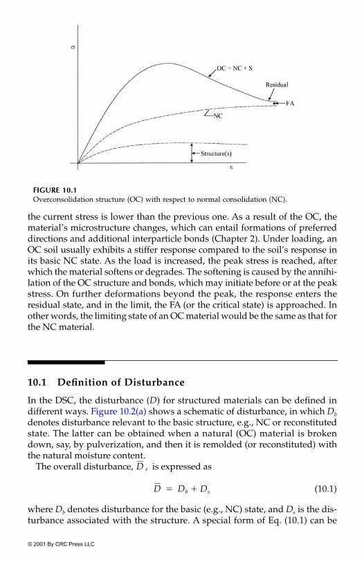
© 2001 By CRC Press LLC
the current stress is lower than the previous one. As a result of the OC, thematerial’s microstructure changes, which can entail formations of preferreddirections and additional interparticle bonds (Chapter 2). Under loading, anOC soil usually exhibits a stiffer response compared to the soil’s response inits basic NC state. As the load is increased, the peak stress is reached, afterwhich the material softens or degrades. The softening is caused by the annihi-lation of the OC structure and bonds, which may initiate before or at the peakstress. On further deformations beyond the peak, the response enters theresidual state, and in the limit, the FA (or the critical state) is approached. Inother words, the limiting state of an OC material would be the same as that forthe NC material.
10.1 Definition of Disturbance
In the DSC, the disturbance (D) for structured materials can be defined indifferent ways. Figure 10.2(a) shows a schematic of disturbance, in which Db
denotes disturbance relevant to the basic structure, e.g., NC or reconstitutedstate. The latter can be obtained when a natural (OC) material is brokendown, say, by pulverization, and then it is remolded (or reconstituted) withthe natural moisture content.
The overall disturbance, , is expressed as
(10.1)
where Db denotes disturbance for the basic (e.g., NC) state, and Ds is the dis-turbance associated with the structure. A special form of Eq. (10.1) can be
FIGURE 10.1Overconsolidation structure (OC) with respect to normal consolidation (NC).
D
D Db Ds��

© 2001 By CRC Press LLC
written as
(10.2a)
in which the first term represents Db, the function f(s) denotes the change(increase or decrease) in disturbance due to the structure, � is the (deviatoric)plastic strain trajectory, and Du, A, and Z are the material parameters. Equa-tion (10.2a) can be simplified such that the response is considered only for thebehavior of the structured state. Then, it is specialized as [Fig. 10.2(b)]
(10.2b)
Alternatively, the disturbance of the material in the basic state, Db, can beadopted as unity; then
(10.2c)
FIGURE 10.2Disturbance due to structure.
D Dub 1 eAb�
Zb�
� f s( )e
As�Zs
���
D f s( )eAs�
Zs�
�
D 1 f s( )eAs�
Zs�
��

© 2001 By CRC Press LLC
Figure 10.2 shows that the structure imposed on the basic state is annihi-lated gradually as the load is applied, and in the limit, it approaches thebasic structure, Db0. An example of the characterization of the compressivebehavior of a structured soil obtained by using the simplified Eq. (10.2c) isgiven subsequently.
Figure 10.3(a) shows the response of a structured material that exhibitshardening, peak, and softening. After the critical or threshold plastic strains,�t(�t ), the internal microstructure of the material can modify due to thestrengthening of bonds as a result of different influences. In the case of dislo-cated silicon under thermomechanical loading, such an influence can arisedue to the locking of dislocations with impurities such as oxygen and nitrogen,in the presence of specific temperatures.
FIGURE 10.3Softening and stiffening responses.

© 2001 By CRC Press LLC
A saturated soil (sand) under cyclic (earthquake) loading can first experi-ence degradation due to the increase in pore water pressures, i.e., decrease inthe effective stress, leading to instability and liquefaction at the critical distur-bance (Dc ) corresponding to plastic strains (�c) after loading cycles (Nc); seeFig. 10.4(a) and (b). Then, in the postliquefaction region, the porous material canexperience drainage with a resultant decrease in the pore water pressure (2).
FIGURE 10.4Liquefaction and postliquefaction behavior of saturated sand.

© 2001 By CRC Press LLC
This can lead to an increase in the strength as the effective stress increases.Hence, the disturbance decreases in the postliquefaction zone (3) [Fig. 10.4(c)].
An asphaltic concrete (used in pavements) is subjected to vehicular trafficload during days, while it can experience healing or increase in stiffness dueto rest periods (during nights) (4). Such healing can be attributed to chemicaleffects as well as unloading, which can result in a decrease in plastic strainsand microcracking. The specific contributions of mechanical unloading andchemical effect are not known precisely. Figure 10.5 shows the effect of restperiods on the flexural stiffness of an asphalt obtained from flexural fatiguetests on beams, with and without rest periods (4). The figure also shows thatthe cycles to fatigue failure (�Nf) increase with rest periods.
In Chapter 2 we discussed the response of a porous chalk that exhibits thebehavior in Fig. 2.10 similar to that in Fig. 10.3. In the case of composite or rein-forced materials, the disturbance can be defined relative to the responses ofthe component materials (Chapter 2).
Examples of the formulation of the DSC for a structured soil, a dislocatedsilicon with oxygen impurities, a reinforced soil and a jointed rock, and healingor stiffening due to unloading are discussed in the remainder of this chapter.
10.2 Structured Soils
Materials such as soils can develop a structure due to natural deposition pro-cesses caused by geological history and by artificial methods such as applica-tion of mechanical load. Such a structure can be defined with respect to thatof the soil in its reconstituted or remolded state, which can be considered torepresent its basic state before the forces causing the change in the structurewere imposed.
In the DSC, the behavior of the reconstituted soil can be treated as the fullyadjusted state, and then the effect of the structure developed can be introduced
FIGURE 10.5Flexural stiffness of asphalt concrete with and without rest periods (4). 2000©John Wiley &Sons Ltd. Reproduced with permission.

© 2001 By CRC Press LLC
as the change in disturbance with respect to the disturbance at the reconsti-tuted state. Then the modified disturbance, , to allow for the structure,which can result in stiffening with respect to the FA state, can be expressedusing Eq. (10.2).
We describe an example of the application of the DSC for naturally or arti-ficially structured soil. The formulation presented here has been reportedby Liu et al. (5). The incremental strain equations for the DSC [Eq. (4.46),Chapter 4] are given by
(10.3a)
where D� is the disturbance function. Liu et al. (5) assumed that the RI repre-sents “zero strain state,” i.e., it is characterized as a perfectly rigid material.Hence, , and Eq. (10.3a) is simplified as
(10.3b)
The disturbance function for the structured soil is expressed as
(10.4)
Hence, the observed strain is given by
(10.5)
The disturbance function can be decomposed in two parts as
(10.6a)
and
(10.6b)
where and are disturbance functions related to volumetric and devi-atoric behavior, respectively, and
(10.7a)
(10.7b)
D
d�˜
a 1 D��( )d�˜
i D� d�˜
c dD˜ � �
˜c
�˜
i�( )� ��
d�˜
i 0˜
�
d�˜
a D� d�˜
c dD� �˜
c� d D��
˜c( )� �
D� D�
�D�
��˜
c----------
T
�˜
c��
d�˜
a D� d�˜
c�
d�va D�v d� v
c�
d�da D�d d�
˜ dc
�
D�v D�d
�v �1 �2 �3� ��
�d2
3------- �1 �2�( )2
�2 �3�( )2�3 �1�( )2
� ��

© 2001 By CRC Press LLC
Here, �i (i � 1, 2, 3) are the principal strains. Thus, the DSC can be formu-lated for the combined volumetric and deviatoric response using Eq. (10.6).Liu et al. (5) considered the compressive behavior of structured soil, based onEq. (10.6a).
Example 10.1 Compression Behavior of a Structured SoilFigure 10.6 shows a schematic of the compression behavior of structured andreconstituted soils expressed in terms of void ratio (e) and ln p, where p isthe mean effective pressure. As the pressure is increased on the structuredsoil, it experiences a process of destructuring during which the soil’s structure(bonds) is annihilated and, in the limit, the soil approaches the reconstitutedstate, at high pressures.
It was assumed that when the pressure p was below the pressure whenyielding occurred, the behavior was elastic, and there was no disturbance. Inother words, disturbance and destructuring occur only due to plastic yieldingbeyond the pressure .
The yielding virgin response beyond was defined using the DSC model,in which the disturbance, [Eq. (10.6a)] was defined based on the observed(compression) behavior of a number of structured soils as [Eq. (10.2c)]
(10.8)
where b is the disturbance index, to represent the structure with reference tothat of the reconstituted soil. In Eq. (10.8), the value of Db in Eq. (10.2) isassumed to be unity relevant to the reconstituted state. A plot of is shownin Fig. 10.2(b), where b � f(s).
Liu et al. (5) presented various versions of the DSC model for the compres-sive behavior: (1) for the case when the (experimental) compression data areavailable in terms of mean effective pressure and volumetric response, and (2)for the case when the data are available in terms of effective vertical or axial
FIGURE 10.6Schematic of compression behavior of reconstituted and structured soils (5). ©John Wiley& Sons Ltd. Reproduced with permission.
py ,i,
py ,i
py ,i
D�v
D�v 1 bpy ,i
p----------
��
D�v

© 2001 By CRC Press LLC
stress ( ) from one-dimensional compression tests. These formulations werebased on the critical-state concept (5–7), and the resulting equations are givenbelow:
Case 1:
(10.9)
Case 2:
(10.10)
where and denote slopes of a virgin curve (Chapter 3), and and denote the slope of an unloading curve on an e � ln p plot.
10.2.1 Validations
The DSC model was used to predict compression behavior of seven differentsoils (5). Typical results for two soils are included here; Table 10.1 shows theirproperties.
For soil 1, the test data were available (8) in terms of mean effective stress,p. Then, Eq. (10.9) was used for the back predictions. For soil 2, the test datawere available (9) in terms of effective vertical stress ( ); hence, Eq. (10.10)was used for the back predictions.
TABLE 10.1
Details of Compression Tests and Parameters
Soil Reference (kPa) b Comments
1. MexicoCity clay
Terzaghi (8) 92.0 1.65 — — Very high void ratio;e � ln p nonlinear
2. Leda clay Quigley and 185.0 4.10 e � ln linearThompson (9) 0.02 0.16
v
d�va
��
1 e�------------- d p
p-------- for p py�
�
1 e�------------- 1 b
py ,i
p----------
�dpp
-------- for p py�
�
d�va
� �v1 e�-------------
dvv
----------- for v v y�
v�
1 e�------------- 1 bv
vy ,i
v------------
�dvv
----------- for v pvy�
�
� v� � � � �v
v
p�y ,i
��
��
�v�
v�
v
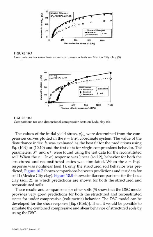
© 2001 By CRC Press LLC
The values of the initial yield stress, , were determined from the com-pression curves plotted in the e � ln coordinate system. The value of thedisturbance index, b, was evaluated as the best fit for the predictions usingEq. (10.9) or (10.10) and the test data for virgin compressions behavior. Theparameters, and , were found using the test data for the reconstitutedsoil. When the e � ln response was linear (soil 2), behavior for both thestructured and reconstituted states was simulated. When the e � lnresponse was nonlinear (soil 1), only the structured soil behavior was pre-dicted; Figure 10.7 shows comparisons between predictions and test data forsoil 1 (Mexico City clay). Figure 10.8 shows similar comparisons for the Ledaclay (soil 2), in which predictions are shown for both the structured andreconstituted soils.
These results and comparisons for other soils (5) show that the DSC modelprovides very good predictions for both the structured and reconstitutedstates for under compressive (volumetric) behavior. The DSC model can bedeveloped for the shear response [Eq. (10.6b)]. Then, it would be possible tosimulate the combined compressive and shear behavior of structured soils byusing the DSC.
FIGURE 10.7Comparisons for one-dimensional compression tests on Mexico City clay (5).
FIGURE 10.8Comparisons for one-dimensional compression tests on Leda clay (5).
py ,i
pv
� � �
vpv

© 2001 By CRC Press LLC
10.3 Dislocations, Softening, and Stiffening
The mechanical behavior of silicon crystals as affected by factors such as dis-location density (N0), temperature (T), strain rate ( ), and impurities such asoxygen and nitrogen may exhibit responses as depicted in Fig. 10.3 (10, 11).
Example 10.2 Dislocated Silicon with ImpuritiesFigure 10.9 shows stress–strain data for silicon crystals under different dislo-cations, temperature, and strain rates reported by Yonenaga et al. (11). It canbe seen that the peak or upper yield stress was not affected significantly forthe dislocation free crystals [Fig. 10.9(a)], while it shows significant increasefor the dislocation, N0 � 1 � as the oxygen concentration increases.Such an effect is attributed to the locking of dislocations by oxygen atoms dis-solved in silica crystals because the dislocations become immobile due to
FIGURE 10.9Stress–strain behavior of silicon doped with different oxygen content (11) (with permission).
�
106 cm 2� ,

© 2001 By CRC Press LLC
impurity locking, while the crystal is kept at elevated temperature under noapplied stress (11).
The prepeak region of the stress–strain response is usually elastoplastic withplastic yielding or hardening, during which the yield stresses increase withplastic deformations (Chapter 7); Fig. 10.9. There occurs a reduction in thestress after the peak stress, often referred to as softening or degradation, whichresults due to the initiation of microcracking (sometimes before the peakstress), and its growth due to the coalescence of microcracks. For some mate-rials, microstructural instability occurs at critical locations or disturbance, Dc,and failure may subsequently occur near the ultimate condition, Du. In thecase of the silicon with impurities, however, the softening may continue up tothe point b in Fig. 10.3(a), and then under the specific combination of N0, T, and
and after the threshold plastic strains (�t), the material exhibits stiffening orhealing response. Often, the stiffening is higher for greater values of the dislo-cation density (N0).
10.3.1 Formulation of DSC Model
Figure 10.3 shows a schematic of the response as a combination of hardening–softening–stiffening behavior. The response, 0–a–b–c, is the basic hardening–softening behavior, which has been characterized before (Chapter 4),using Eq. (4.1) as
(10.11)
In this case, the disturbance, D, increases with (plastic) deformation, shownas 0–a–b, Fig. 10.3(b).
In the case of the stiffening response beyond point b, the material exhibitshigher stress-carrying capacity and is assumed to approach an asymptoticvalue (near d). Then, during stiffening, the disturbance decreases, as depictedby b–d in Fig. 10.3(b).
For the combined hardening–softening–stiffening response, the modifieddisturbance function, in Eq. (10.2) is expressed as (12)
(10.12)
where Dub , Ab , and Zb are parameters for the basic softening behavior; As
and Zs are parameters related to the stiffening response; and is given by
(10.13)
where Dus is the ultimate disturbance corresponding to the limiting stiffening
�,
d˜
a 1 D�( )C˜
i d�˜
i Dcc d�˜
c dD ˜
c˜
c�( )� ��
D,
D Dub 1 Ab�DZb�( )exp�{ } 1 As�D
Zs�( )exp�{ }�[ ]�
,
0 if �D �t�
Dus
Dub--------- if �D �t�
�

© 2001 By CRC Press LLC
response, and �t is the threshold value of the deviatoric plastic strain trajec-tory when the stiffening initiates.
With the modified disturbance, , the DSC incremental equations are mod-ified as
(10.14)
10.3.2 Validation
Applications of the DSC model for the basic softening behavior exhibited bysilicon crystal (ribbons) with relatively low dislocation densities (N0 � 2 �
) and low oxygen concentration (C0 � atoms� ) (10) aregiven in Example 7.16, Chapter 7; this material does not exhibit stiffeningbehavior. Here, we present application of the modified DSC equation (10.14)for characterizing the behavior of dislocated silicon with high levels of dislo-cation densities (N0) and oxygen concentration (C0), which exhibits the stiff-ening response. Figure 10.9 shows laboratory test results for such silicondoped with oxygen as reported by Yonenaga et al. (11).
The stress–strain data (Fig. 10.9) were used to find the parameters for eachindividual curve for the dislocation-free (N0 � 0) and dislocation (N0 � 1 �
conditions. The elastic modulus, E (slope at the origin), was foundfor each stress–strain curve. Its average value for T � 800�C was found to be2.45 � Pa, and for T � 900�C, it was found to be 1.67 � Pa. The RIresponse was assumed to be linear elastic.
The disturbance parameters were found using procedures given in Chap-ters 4 and 7 and are shown in Tables 10.2(a) and (b) for T � 900�C and 800�C,respectively. The parameters were expressed as functions of the oxygen con-centration, C0, using the following relations:
(10.15)
where the subscript r denotes reference concentration, C0 � 1 �accordingly, e.g., Abr is the value of Ab at C0 � 1 � Table 10.2(c)shows the parameters in Eq. (10.15). The parameters obtained from the testwith C0 � 4 � were not used in the “average” relations [Eq. (10.15)];this test was used as an independent validation.
D
d˜
a 1 D�( )C˜
i d�˜
i DC˜
c d�˜
c dD ˜
c˜
i�( )� ��
103 cm 2� 1014 cm3
1016 cm 2� )
109 109
Ab C0( ) AbrC0
Cr------
�1
�
Zb C0( ) ZbrC0
Cr------
�2
�
As C0( ) AsrC0
Cr------
�3
�
Zs C0( ) ZsrC0
Cr------
�4
�
107 cm 3� ;107 cm 3� .
1017 cm 3�

© 2001 By CRC Press LLC
The laboratory curves were predicted by integrating Eq. (10.14), in whichthe RI behavior, was defined based on linear elastic response, and the FAresponse, was based on the bulk modulus (K ). The disturbance function
in Eq. (10.12) was used with the parameters shown in Table 10.2.Figures 10.10(a) and (b) show comparisons between predictions and test
data for two individual responses: (1) N0 � 0.0, C0 � 2.5 � T �900�C, and (2) N0 � 1 � C0 � 1.5 � T � 800�C, respec-tively. The parameters used for these predictions were relevant to the individ-ual stress– strain data.
Figures 10.11(a) and (b) show comparisons between predictions and testdata for two independent tests: (1) N0 � 0.0, C0 � 4 � T � 900�C,and (2) N0 � 1 � C0 � 4 � T � 800�C. Here the averageparameters were used to predict independent tests that were not used in find-ing the parameters. It can be seen from Figs. 10.10 and 10.11 that the DSCmodel provides very good predictions of the behavior of dislocated silicondoped with oxygen, as affected by C0, N0, and T.
TABLE 10.2(a)
Parameters for N0 � 0 at T � 900�C
C0 �Dub Dus Ab As Zb Zs
2.5 0.5909 0.6558 1.1099 23.9657 �3.6464 1.1196 2.08444.0 0.3174 0.6397 2.0156 15.0097 �2.1515 0.7941 1.73775.5 0.4815 0.6667 1.3846 7.4037 �1.9060 0.6109 1.68899.0 0.4661 0.6260 2.0156 3.5548 �1.2710 0.4148 1.4809
TABLE 10.2(b)
Parameters for N0 � 1 � at T � 800�C
C0 �Dub Dus Ab As Zb Zs
1.5 0.4497 0.7512 0.5987 4.0748 �7.2044 0.5637 1.98194.0 0.5629 0.4545 1.2385 8.3227 �3.7178 0.6800 1.84436.5 0.6624 0.8112 0.7672 11.8467 �2.6796 0.7462 1.77979.0 0.7017 — — 15.0097 �2.1515 0.7941 1.7377
TABLE 10.2(c)
Parameters in Eq. (10.15)
Temperature (�C) Abr Asr Zbr Zsr �1 �2 �3 �4
800 4.0785 7.2044 0.5638 1.9820 0.7272 �0.6745 0.1912 �0.07341900 51.2980 5.5514 1.6577 2.3889 �1.4898 �0.8228 0.7683 �0.2669
1017
cm 3� �
1016 cm 2�
1017
cm 3� �
C˜
i,C˜
c,D
1017 cm 3� ,106 cm 2� , 1017 cm 3� ,
1017 cm 3� ,10 6 cm 2� , 1017 cm 3� ,

© 2001 By CRC Press LLC
10.3.3 Disturbance and Dislocation Density
It was also shown by Desai et al. (12) that disturbance in the DSC and dislo-cation density can be correlated. The latter is given as [Eq. (3.25a)], Chapter 3(10, 12)
(10.16a)
where k is Boltzmann’s constant (� 8.617 � evK); is the backstress, Q is the Peierl’s energy (� 2.17 ev), , p, and r are material constants(� 3.1 � , 1.1, and 1.0, respectively), k0 � B0/�0, B0 is mobility (� 4.30 �
m�s), T is absolute temperature, �0 � N� denotes the observedstress, the overdot denotes time derivative, and m denotes any point. Byusing the stress-based disturbance [Eq. (3.7), Chapter 3], Eq. (10.16a) can be
FIGURE 10.10Comparisons between observed and predicted individual responses (12) (with permission).
Nm KNmk0 J2Da
Nm�( )p�r
e Q�kT��
10 5� Nm
K10 4�
104 107 m2, J2Da

© 2001 By CRC Press LLC
expressed as
(10.16b)
where denotes the RI shear stress.Figure 10.12 shows the plot of the dislocation density vs. axial strain for the
test (10) in Fig. 7.44, Chapter 7, for the curve T � 1100�C, � 4.8 �and N0 � 1.8 � This plot is obtained by integrating Eqs. (10.16a) and(10.16b); here the values of disturbance at various points are used inEq. (10.16b) for the DSC predictions. It can be seen that both Eqs. (10.16a) and
FIGURE 10.11Comparisons between observed and predicted independent responses (12) (with permis-sion).
Nm KNmk0 1 D�( ) J2Di
Nm )�[ ]p��
e Q�kT��
J2Di
� 10 4� s 1� ,105 cm 2� .

© 2001 By CRC Press LLC
(10.16b) show essentially the same results, implying that the disturbance anddislocation densities bear a correlation.
10.4 Reinforced and Jointed Systems
Materials are often reinforced to enhance their deformation and strengthproperties, e.g., reinforced concrete, reinforced earth, and composites (metallic,ceramic, etc.). Some materials involve joints or interfaces that exist before theload is applied or are induced during loading. Structure-foundation systemsand jointed rocks are examples of the former, whereas the latter can occur inany material that experiences microcracking leading to macro- or finite-sizedcracks. In the case of joints, the material is usually weaker than the parent orsolid material parts; see Fig. 10.13.
Reinforced and jointed material systems can be characterized using the DSCin two ways: (1) by expressing the observed behavior of the equivalent rein-forced or jointed composite in terms of the behavior of the solid and the joint(Fig. 10.13), or (2) by treating the body as made of solid, interfaces or joints,and then introducing their responses individually, say, in the finite-elementanalysis.
10.4.1 Equivalent Composite
In the case of the equivalent composite, the observed or actual behavior of thecomposite can be expressed as (Chapter 2)
(10.17)
FIGURE 10.12Comparison of dislocation density vs. strain with Eq. (10.16): independent tests (12) (withpermission).
d˜ m
a 1 Dm�( )d˜ s
a Dm d˜ j
a dDm ˜ j
a˜ s
s�( )� ��

© 2001 By CRC Press LLC
where and denote the observed stresses in the composite, solid,and joint�interface, respectively [Fig. 10.13(a)]. Then it will be necessary toconduct laboratory tests on specimens of the solid and joint to measure anddefine their observed behavior. The observed behavior of the solid, andthat of the joint, can be expressed in terms of the responses of their respec-tive RI and FA states:
(10.18a)
and
(10.18b)
where and are the RI stresses for the solid and joint, respectively, and are the FA stresses for the solid and joint, respectively, and Ds and Dj
are disturbances for the solid and joint behavior, respectively [Fig. 10.13(b)].
FIGURE 10.13Representations for composite material systems.
˜ m
a , ˜ s
a, ˜ j
a
sa,
ja,
dsa 1 Ds�( )ds
i Ds dsc dDs s
cs
i�( )� ��
d ja 1 Dj�( )d j
i Dj d jc dDj j
c j
i�( )� ��
si
ji
sc
jc
© 2001 By CRC Press LLC
With the foregoing formulation in the FE procedure, the elements in themesh will be considered as a composite containing a joint or interface withsurrounding elements [Fig. 10.13(a)]. The equations for such a compositeelement can be expressed as
(10.19)
where the stiffness
(10.20)
where denotes the applied load, and is the constitutive matrix forthe composite element, which is expressed in Eq. (10.17).
10.4.2 Individual Solid and Joint Elements
In this approach, the structure is divided into solid and joint or interfaceelements. Then the behavior of each is characterized using the DSC model.This method is similar to the standard FE method in which solid and jointregions are treated as individual elements with definition of properties formaterial (solid or joint) for each element.
Example 10.3 Reinforced Earth and Jointed RockWe present an example of reinforced earth in which both precedingapproaches were used (13). Figure 10.14 shows the finite-element mesh for alaboratory triaxial test with cylindrical specimen reinforced by a single layerof nonwoven geotextile (R1NW) at the midheight of the specimen. Tests werealso performed with two layers of the nonwoven geotextile placed at onethird and two thirds of the specimen’s height (R2NW), and two layers ofwoven geotextile at one third and two thirds height (R2W). A number of tri-axial tests were also performed for the natural sand specimens, without rein-forcement. The soil was Enmore sand procured from the coastal area in Indianear the City of Chennai (old Madras). The physical properties of the sandare as follows:
Specific gravity � 2.64Uniformity coefficient � 1.63Median size, D50 � 0.60 mmMaximum dry density � 18.0 KN�
Minimum dry density � 16.0 KN�
k˜mdq
˜m
dQ˜
m�
k˜m B
˜TC
˜ ma B
˜dV��
dQ˜
m C˜ m
a
m3
m3

© 2001 By CRC Press LLC
The tests were performed under three confining pressures in the range of100 to 300 kPa, with different stress paths, compression �CTC (Sr � 1.00) andextension � RTE (Sr � �1.0); see Chapter 7, Fig. 7.13.
TABLE 10.3(a)
Material Parameters for Natural and Reinforced Soils
Parameter Natural SoilReinforced Soil
(R1NW)Reinforced Soil
(R2NW)Reinforced Soil
(R2W)
Elastic constantsk 600.00 500.00 230.00 690.00n 0.95 0.96 1.06 0.90� 0.34 0.37 0.36 0.34
Ultimateparameters
� 0.071 0.072 0.088 0.089� 0.610 0.687 0.727 0.667
Phase changeparameter, n
2.54 2.98 3.07 2.90
Hardeningparameters
a1 0.366 � 0.405 � 0.397 � 0.273 ��1 0.711 1.611 1.327 0.721
Nonassociativeparameter, �
0.228 0.276 0.242 0.257
From Ref. 13, ©John Wiley & Sons Ltd. Reproduced with permission.
TABLE 10.3(b)
Material Parameters of Interface Between Soil and Nonwoven and Woven Geotextiles
ParameterNonwovenGeotextile
Woven Geotextile
Elastic constants (k N�m2�m) Ks 3,000 8,000Kn 60,000 90,000
Ultimate parameters � 0.722 0.656Phase change parameter n 2.84 2.50Hardening parameters a1 0.098 0.253
�1 0.675 0.241Nonassociative parameter � 0.875 0.802
See Chapter 11 for details of interfaces.
TABLE 10.3(c)
Parameters for Geotextile Reinforcement
Properties Nonwoven Geotextile Woven Geotextile
Material�color Polypropylene�white Polypropylene�whiteThickness (mm) 2.8 0.64Stiffness modulus (k N�m) 23.13 660Yield strength (k N�m) 11.65 19.93
10 3� 10 5� 10 4� 10 3�

© 2001 By CRC Press LLC
Tests for the sand-reinforcement interfaces were conducted by using a testbox of 6.0 � 6.0 cm size, in which the lower half of the box contained a steelblock over which the geotextile was wrapped and fixed. The upper half of thebox was filled with dry sand. Normal stresses of 50, 100, and 100 kPa wereused with shear displacement rate of 0.25 mm/min.
The elastic moduli and the yield strength of the geotextile were determinedfrom tension tests conducted by using a Universal Testing Machine (13).
The HISS �0- and �1-plasticity models (Chapter 7) were used to characterizethe behavior of the sand and interface (Chapter 11), while the woven andnonwoven reinforcements were modelled using the von Mises yield crite-rion. Table 10.3 (a), (b), and (c) shows the HISS parameters for the naturaland reinforced sand, interface, and the parameters for the geotextiles,respectively. In the case of the sand, the elastic modulus, E, was expressed asa function of the confining stress, 3, as
(10.21)
where k and nare parameters and pa is the atmospheric pressure constant.Analysis The observed hardening behavior of the natural and reinforced
soil with woven geotextile is compared in Fig. 10.15 (a) and (b) for the woven
FIGURE 10.14Finite-element discretization of reinforced soil sample (13). ©John Wiley & Sons Ltd. Repro-duced with permission.
E kpa3
pa-----
n
�
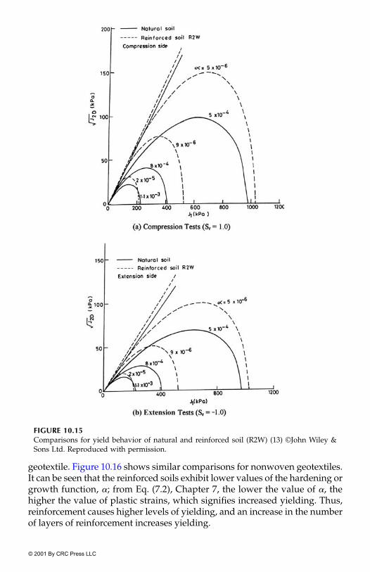
© 2001 By CRC Press LLC
geotextile. Figure 10.16 shows similar comparisons for nonwoven geotextiles.It can be seen that the reinforced soils exhibit lower values of the hardening orgrowth function, �; from Eq. (7.2), Chapter 7, the lower the value of �, thehigher the value of plastic strains, which signifies increased yielding. Thus,reinforcement causes higher levels of yielding, and an increase in the numberof layers of reinforcement increases yielding.
FIGURE 10.15Comparisons for yield behavior of natural and reinforced soil (R2W) (13) ©John Wiley &Sons Ltd. Reproduced with permission.

© 2001 By CRC Press LLC
Figure 10.17 shows yielding behavior for the interfaces with nonwoven andwoven reinforcements. It indicates that the growth function, �, is lower fornonwoven geotextile; i.e., the yielding is higher for the nonwoven geotextilecompared to that for the woven geotextile.
10.4.3 Validation for Test Results with HISS Model and FE Method
The triaxial stress–strain–volume change behavior was predicted using twomethods: SPM and FEM. In the SPM method, the specimen was treated as anequivalent composite element. The predictions were obtained by integratingthe incremental constitutive equations [Eq. (10.17)], in which the HISS param-eters for the composite reinforced soil were used; see Table 10.3.
In the FEM, the specimen was considered to be made of three components:natural soil, reinforcement (geotextile), and interface between the soil andreinforcement. The properties of individual components were provided in theFEM (Table 10.3).
The validations were obtained by using (average) parameters for the testswhich were used for finding the parameters (Group A). Then validations wereobtained for independent tests not used for finding the parameters (Group B).Only typical results are given below.
Figures 10.18 and 10.19 show comparisons between predictions and testdata for the reinforced specimen (R2W) for the reduced triaxial extension(RTE) and triaxial compression (TC) stress paths (Fig. 7.13), respectively, forGroup A and Group B analyses. It can be seen that both the SPM and FEM pre-dictions correlate well with the test behavior.
FIGURE 10.16Comparisons of yield behavior for natural soil and reinforced soil, R1NW and R2NW:extension test (Sr � �1.0)(13). ©John Wiley & Sons Ltd. Reproduced with permission.

© 2001 By CRC Press LLC
10.4.4 Jointed Rock
The FEM approach, in which each component is treated individually, wasapplied to analyze the (laboratory) behavior of jointed rock masses using theDSC model (14). It was found that the DSC model provided very good corre-lation with the laboratory behavior of a rock mass with three inclined joints.
The foregoing results show that the special version, the HISS plasticitymodel of the DSC, provides satisfactory simulation of the behavior of the rein-forced soil. Both the equivalent composite and the component approaches canbe used for characterizing the behavior of a reinforced composite. The DSCmodel including softening or degradation would also provide satisfactory results,as was reported by Chia et al. (14).
Characterization of soils and interfaces, and FE predictions for a Tensar(plastic) reinforced retaining wall using the DSC, are given in Chapter 13.
FIGURE 10.17Plots of yield surfaces for soil-reinforcement interfaces (13). ©John Wiley & Sons Ltd. Re-produced with permission.
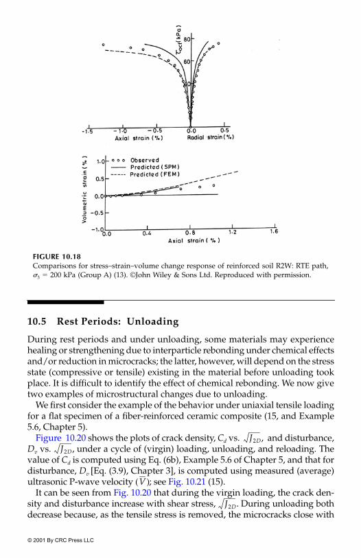
© 2001 By CRC Press LLC
10.5 Rest Periods: Unloading
During rest periods and under unloading, some materials may experiencehealing or strengthening due to interparticle rebonding under chemical effectsand/or reduction in microcracks; the latter, however, will depend on the stressstate (compressive or tensile) existing in the material before unloading tookplace. It is difficult to identify the effect of chemical rebonding. We now givetwo examples of microstructural changes due to unloading.
We first consider the example of the behavior under uniaxial tensile loadingfor a flat specimen of a fiber-reinforced ceramic composite (15, and Example5.6, Chapter 5).
Figure 10.20 shows the plots of crack density, Cd vs. and disturbance,Dv vs. under a cycle of (virgin) loading, unloading, and reloading. Thevalue of Cd is computed using Eq. (6b), Example 5.6 of Chapter 5, and that fordisturbance, Dv [Eq. (3.9), Chapter 3], is computed using measured (average)ultrasonic P-wave velocity ; see Fig. 10.21 (15).
It can be seen from Fig. 10.20 that during the virgin loading, the crack den-sity and disturbance increase with shear stress, During unloading bothdecrease because, as the tensile stress is removed, the microcracks close with
FIGURE 10.18Comparisons for stress–strain–volume change response of reinforced soil R2W: RTE path,3 � 200 kPa (Group A) (13). ©John Wiley & Sons Ltd. Reproduced with permission.
J2D,J2D,
V( )
J2D.

© 2001 By CRC Press LLC
a consequent reduction in the disturbance. Upon reloading, both Cd and Dv
increase again; at the end of reloading, the virgin loading response resumes.Thus, during unloading, as the disturbance decreases, the material exhibits ahealing or stiffer response [Eq. (10.14)].
On the other hand, if the material is under compressive stress state whenunloading occurs, the situation can be different. Figure 10.22 illustrates thisphenomenon for the behavior of a cemented sand tested under multiaxialcompressive loading, e.g., the CTC stress path (1 > 2 � 3) (Fig. 7.13,Chapter 7). Figure 10.23 shows the plot of measured vs. for thecemented sand used to compute Dv.
During the virgin loading, both Cd and Dv (Fig. 10.22) increase. Underunloading, both increase because as the compressive stress is removed, themicrocracks can experience opening, resulting in an increase in the distur-bance. During reloading, Cd and Dv first decrease due to the coalescence ofmicrocracks, and then they increase. Thus, mechanical healing during unload-ing is not present, except during a part of the reloading.
Hence, the existence of healing or stiffening due to mechanical unloadingdepends on the stress state. Healing due to chemical effects can occur simulta-neously during unloading, but requires additional studies and research for itsdefinition and quantification.
FIGURE 10.19Comparisons for stress–strain–volume change response of reinforced soil R2W: TC path,3 � 200 kPa (Group B) (13). ©John Wiley & Sons Ltd. Reproduced with permission.
V J2D

© 2001 By CRC Press LLC
References
1. Desai, C.S., “Consistent Finite Element Technique for Worksoftening Behavior,”Proc. Int. Conf. on Comp. Meth. in Nonlinear Mech., J.T. Oden (Editor), Univ. ofTexas, Austin, TX, 1974.
2. Vaid, Y.P. and Thomas, J., “Liquefaction and Post Liquefaction Behavior ofSand,” J. of Geotech. Eng., ASCE, 121, 2, 1995, 163–173.
3. Desai, C.S., Park, I.J., and Shao, C., “Fundamental Yet Simplified Model forLiquefaction Instability,” Int. J. Num. Analyt. Meth. Geomech., 22, 1998, 721–748.
[
FIGURE 10.20Variations of Dv and Cd for fiber ceramic (15) (with permission).
FIGURE 10.21Average ultrasonic P-wave velocity for fiber-reinforced ceramic (15) (with permission fromElsevier Science).

© 2001 By CRC Press LLC
FIGURE 10.22Variations of Dv and Cd for CTC30-cemented sand (15) (with permission from ElsevierScience)..
FIGURE 10.23Average ultrasonic P-wave velocity for cemented sand (15) (with permission from ElsevierScience)..

© 2001 By CRC Press LLC
4. Kim, Y.R., Lee, H.J., Kim, Y., and Little, D.N., “Mechanistic Evaluation ofFatigue Damage Growth and Healing of Asphalt Concrete: Laboratory andField Experiments,” Proc. 8th Int. Conf. on Asphalt Pavements, Seattle, WA, USA,1987, 1089–1108.
5. Liu, M.D., Carter, J.P., Desai, C.S., and Xu, K.J., “Analysis of the Compressionof Structured Soils Using the Disturbed State Concept,” Int. J. Num. Analyt.Methods in Geomech., 24, 8, 2000, 723–735.
6. Scofield, A.N. and Wroth, C.P., Critical State Soil Mechanics, McGraw Hill,London, U.K., 1968.
7. Liu, M.D. and Carter, J.P., “On the Volumetric Deformation of ReconstitutedSoils,” Int. J. Num. Analyt. Meth. Geomech., 24, 2, 2000, 101–133.
8. Terzaghi, K., “Fifty Years of Subsoil Exploration,” Proc. 3rd Int. Conf. on SoilMech. and Found. Eng., 1953, 227–238.
9. Quigley, R.M. and Thompson, C.D., “The Fabric of Anisotropic ConsolidatedSensitive Marine Clay,” Canadian Geotech. J., 3, 1966, 61–73.
10. Dillon, G.W., Tsai, C.T., and DeAnglis, R.J., “Dislocation Dynamics During theGrowth of Silicon Ribon,” J. of Appl. Physics, 60, 5, 1986, 1784–1792.
11. Yonenaga, I., Sumino, K., and Hoshi, J., “Mechanical Strength of Silicon Crystalsas a Function of the Oxygen Concentration,” J. of Appl. Physics, 56, 8, 1984,2346–2350.
12. Desai, C.S., Dishongh, T.J., and Deneke, P., “Disturbed State Constitutive Modelfor Thermomechanical Behavior of Dislocated Silicon with Impurities,” J. ofAppl. Physics, 84, 11, 1998, 5977–5984.
13. Varadarajan, A., Sharma, K.G., and Soni, K.M., “Constitutive Modelling of aReinforced Soil Using Hierarchical Model,” Int. J. Num. Analyt. Meth. Geomech.,23,3, 1999, 217–241.
14. Chia, J., Chern, J.C., and Lin, C.C., “DSC Finite Element Modeling of Progres-sive Failure in Jointed Rock,” Proc. 9th Int. Conf. on Computer Meth. and Advancesin Geomech., Yuan, J.X., (Editor), Balkema, Rotterdam, 1997.
15. Desai, C.S. and Toth, J., “Disturbed State Constitutive Modeling Based onStress–Strain and Nondestructive Behavior,” Int. J. Solids and Struct., 33, 11,1996, 1619–1650.

© 2001 By CRC Press LLC
11The DSC for Interfaces and Joints
CONTENTS11.1 General Problem11.2 Review
11.2.1 Comments11.3 Thin-Layer Interface Model11.4 Disturbed State Concept
11.4.1 Relative Intact Behavior11.4.2 Stress-Displacement Equations11.4.3 Elastoplastic Models11.4.4 Fully Adjusted State11.4.5 FA as the Critical State
11.5 Disturbance Function11.6 Incremental Equations
11.6.1 Specializations11.6.2 Alternative DSC Equations
11.7 Determination of Parameters11.7.1 Mathematical and Physical Characteristics of the DSC11.7.2 Regularization and Penalty
11.8 Testing11.9 Examples
11.9.1 Creep Behavior11.9.2 Testing
11.10 Computer Implementation
The subject of contacts between two similar or dissimilar materials has beenstudied for a long time. The classical friction laws by Coulomb and Amontonsconsidered the case of dry friction between (rigid) bodies. Subsequently, the pur-suit for understanding the complex response at contacts as affected by manypractical factors beyond those considered in the classical laws has continued.
In engineering systems contacts are often referred to as interfaces or jointsbetween two materials. Such discontinuities may preexist or are induced ina deforming material system. Existence of discontinuities in a materialbody whose parts around and beyond the discontinuities may be continu-ous can lead the overall system to be discontinuous. Hence, the theories

© 2001 By CRC Press LLC
based on continuum mechanics may not be applicable to characterize itsresponse. As described in Chapter 2, an initially continuous body mayexperience internal microcracking during loading. Up to a certain extent ofmicrocracks, the material may still be treated as continuous. However, themicrocracks often coalesce and lead to zones of macrolevel fractures. As aresult, the material may no longer be treated as a continuum. In fact, suchfinite-fracture discontinuities may represent interfaces or joints and need tobe treated as such.
11.1 General Problem
Contacts can occur in metals, ceramics, concrete, rocks and soils, composites,and structure-medium (soil or rock) combinations. In mechanical and aero-space engineering, particularly in machinery and aircraft structures, metal-to-metal contacts are common, and behavior is often treated under the subjectof tribology, involving motions and resulting wear, tear, and degradation. Incivil engineering, such contacts refer to interfaces in structures and geologicfoundations, between concrete and reinforcement, and joints in rock masses.Examples of contacts in the electronic industry can involve interfaces andjoints in electronic assemblies such as chip-substrate systems.
Although a number of models have been proposed for the contact prob-lem, its behavior has not yet been fully understood and characterized, par-ticularly when we consider the number of significant factors that influencethe behavior. In the following, we provide a brief review of various modelsbefore describing the rationale for the development and use of the modelsbased on the DSC.
11.2 Review
The subjects of contacts, friction, interfaces and joints involve extensiveresearch and publications. Comprehensive reviews are available in (1–8). Theobjective here is to provide a limited review, particularly with respect to con-stitutive models leading to the development of the DSC.
Amontons’ (9) and Coulomb’s law of friction can be considered to be thefirst formal constitutive model to describe the response of two bodies in con-tact [Fig. 11.1(a)]. The law is expressed as
(11.1)
where F is the tangential or shear force parallel to the plane of contact, �is the coefficient of friction, and N is the force normal to the contact with
F �N�

© 2001 By CRC Press LLC
nominal area A0. The above law is valid for dry friction between rigid bodies,assumes � to be constant, and provides a pointwise description leading todefinition of gross sliding of one body relative to the other. In reality, however,the contact involves mated or nonmated asperities [Fig. 11.1(b)] and the bod-ies in contact can be deformable. As a result, the pointwise or local definitionis not sufficient, and consideration needs to be given to nonlocal effects dueto factors such as nonuniform properties and lack of complete contact. Thelatter would require that the contact area be smaller than the nominal area,A0, and its effect on the behavior needs to be considered.
For including elastic component of response, Archard (10) proposed thefollowing law:
(11.2)
where m is the exponent whose value varies between 2�3 and 1; for purelyelastic behavior, m � 2�3, and for ductile contacts m � 1.
Oden and Pires (11) have discussed the limitations of the Coulomb frictionlaw, in particular its local and pointwise character, and presented variationalprinciples by treating the materials as elastic. The law in Eq. (11.1) was mod-ified as
(11.3a)
where s is the average shear strength of the interface and Ar is the weightedactual contact area, given by
(11.3b)
FIGURE 11.1Schematic of contact and asperities.
A
F �Nm�
F Ar� s
Ar A1 A2…�N1
p0------� �
N2
p0------ …� �
Np0-----�

© 2001 By CRC Press LLC
where A1, A2 … are the contact areas of individual deforming asperities, N1,N2 … are the normal loads on the asperities, and p0 is the approximately con-stant local plastic yield pressure. Substitution of Ar in Eq. (11.3a) gives
(11.3c)
Here s�p0 � �. Thus, F is defined over the weighted area, Ar.In the general areas of friction and contact mechanisms, models based on
strength, limit equilibrium, elastic and classical elastoplastic theories havebeen presented in (1, 2, 4, 6–8, 12–18). In the context of interfaces in structure-medium (soil) and joints in rock, models based on similar and advanced con-cepts have been presented in (3, 5, 19–42).
11.2.1 Comments
As indicated earlier, a number of significant factors influence the behavior atinterface or joint. They include nonlocal considerations, particularly withrespect to the normal behavior, nonlinear effects involving elastic, plastic andcreep strains, microcracking, degradation and softening, stiffening or healing,existence of filler materials (oxides, gouge, etc.), fluids and type of loading(static, cyclic, environmental, etc.). Although the foregoing available modelsallow for strength, elastic, and limited plasticity response, they usually do notallow for factors such as continuous yielding or hardening, microcracking andsoftening leading to postpeak degradation, stiffening, and viscous (time)effects. The objective here is to present the unified DSC model that allows forthese factors, in addition to those included in previous models. It is also notedthat many of the previous models can be derived as special cases of the DSC.
It is felt that the interface behavior needs to be treated as a problem in consti-tutive modelling in which the foregoing factors are integrated. This is in contrastto some of the previous models, which have treated contact or interface behav-ior by introducing constraints (kinematic and�or force) to allow for the effects ofspecial characteristics such as relative motions (sliding, debonding, etc.).
Another important issue is the implementation of the models in solution(computer) procedures with due consideration to factors such as robustness,accuracy, and stability of the numerical predictions. This aspect is handled byusing the concept of the thin-layer element, in which the interface zone is sim-ulated as a thin zone of finite thickness, t (36). In the finite-element procedure,the interface zone is treated as a regular element whose constitutive behavior(with the DSC) is defined based on appropriate laboratory tests using specialshear testing devices.
Models based on the DSC that include elastic, plastic, and creep deforma-tions, microcracking, and (asperity) degradation response have been pre-sented in (42–51). The DSC approach allows for the nonlocal effects andcharacteristic dimension and hence leads to computations that are unaf-fected by spurious mesh dependence (52–54). It may be mentioned that
F sp0-----N �N� �

© 2001 By CRC Press LLC
these models allow realistic characterization of the normal response dis-cussed before (11, 12, 36–39, 41) and the coupled shear and normal response.Particular attention is given here to the (laboratory) measurements of the nor-mal response (55), which is discussed subsequently under testing.
The following descriptions include the DSC models for interfaces andjoints, laboratory testing for the calibration of material parameters, andimplementation of the models in numerical procedures using the thin-layerelement. The latter is described first, as the DSC is formulated with respect tothe thin-layer simulation of interfaces and joints.
11.3 Thin-Layer Interface Model
An interface can involve a number of configurations. The interface betweentwo metallic bodies can be considered clean in the sense that there is no thirdmaterial between them. Then the smeared interface zone can entail differentlevels of roughness defined by the surface (microlevel) asperities [Fig. 11.2(a)].The contact can be very rough to medium-rough to smooth, depending on thecharacteristics (height, length) of irregular asperities. It may be noted thateven a “smooth” contact involves asperities at different levels (macro, micro,etc.); hence, an ideally smooth surface is essentially hypothetical.
It may happen that when two bodies made of different materials are in con-tact, like steel (pile) and soft clays [Fig. 11.2(b)], there exists a finite “smeared”zone between the two that behaves as an interface [Fig. 11.2(e)].
In the case of rock joints, it can happen that the contact is filled with a third(e.g., gouge) material that acts as a bulk interface [Fig. 11.2(c)]. Similar situa-tions occur in the case of chip-substrate system joined together, say, by sol-ders. Here, the filled zone can be treated as the bulk interface [Fig. 11.2(d)]. Itmay be noted, however, that in Fig. 11.2(b), (c), and (d), other interfaces occurbetween the material in the interface and the bodies in contact, which mayinvolve additional considerations such as diffused layers, intermetallics, andsurface effects. These are not considered at this time.
The objective herein is to present a model for the bulk interface or joint thatcan provide a realistic simulation of relative motions between the two bodies.The interface zone is referred to as thin-layer (36, 56) with thickness, t, that canbe treated as equivalent or smeared zone between two materials [Fig. 11.2(e)].If characterized appropriately, it can provide, in a weighted sense, model(s)for the response at the interface. Even in the case of clean contact [Fig. 11.2(a)],it can be possible to develop the dimension (thickness) of the equivalent“smeared” zone, as affected by the asperities, to represent the interfacebehavior. Thus, in all cases in Fig. 11.2, it is assumed that the interface zonecan be represented by an equivalent dimension with thickness, t [Fig. 11.2(e)].
Then the vital question arises as to how to determine the thickness, t. Thiscan be difficult. One of the direct ways would be to perform tests in which the

© 2001 By CRC Press LLC
deformation behavior at the interface is measured, and its significant dimen-sion (t) is determined. Both nondestructive and mechanical testing are possible.In the case of nondestructive tests such as X-ray computerized tomography andacoustic methods, it can be possible to measure the dimensions of the influ-ence zones around the asperities. It is also possible to perform integratednumerical (finite-element) predictions and (laboratory) observations todevelop empirical criteria for defining the thickness, t (36, 56). We shall dis-cuss these aspects later.
FIGURE 11.2Examples of interfaces and joints.

© 2001 By CRC Press LLC
11.4 Disturbed State Concept
Now, as the interface is represented by an equivalent thickness, t [Fig. 11.3(a, b)],it can be treated as a deforming material element that is composed of the rel-ative intact (RI) and fully adjusted (FA) parts. The task now is to define RI andFA behavior for the interface zone.
11.4.1 Relative Intact Behavior
The RI behavior can be represented by using theories such as linear (nonlin-ear) elasticity, elastoplasticity (�0-model for interfaces and joints), ther-moelastoplasticity, and thermoviscoplasticity (Chapters 3–10).
If the (linear) theory of elasticity is used, the RI behavior can be simulatedusing two moduli, shear stiffness, ks, and normal stiffness, kn (Fig. 11.4). Thevalues of these moduli can depend on such factors as the (initial) normalstress (�n0) and roughness (R0). Thus,
(11.4a)
(11.4b)
FIGURE 11.3Thin-layer element and material parts in RI and FA states.
ks ks� �n0, R( )
kn kn� �n0, R( )

© 2001 By CRC Press LLC
11.4.2 Stress-Displacement Equations
For the two-dimensional idealization [Fig. 11.3(c)], the incremental equationsfor the RI behavior with the nonlinear piecewise elastic response areexpressed as
(11.5a)
where � and �n are the shear and normal stresses, respectively, the superscriptt denotes tangent shear and normal stiffnesses, ur and vr are the relative shear
FIGURE 11.4Schematics of shear and normal behavior.
d�
d�n
i ksst ksn
t
knst knn
t�
idur
dvr
i

© 2001 By CRC Press LLC
and normal displacements, respectively, i denotes RI or continuum response,and d denotes an increment. If it is assumed that the elastic shear and normalresponses are uncoupled, Eq. (11.5a) will reduce to
(11.5b)
or
(11.5c)
where d � [d� d�n], d � [dur dvr], and is the interface or joint tangentconstitutive matrix.
As discussed earlier, the net contact area involves contacts at the asperitiesbetween the two bodies and is usually smaller than the nominal or total areaof the contact, A0. In order to account for the nonlocal effects, it is necessaryto introduce weighting functions. In the DSC, such weighting is introducedthrough the disturbance function, D (see later). However, based on the nom-inal area, the shear and normal stress are first defined as
(11.6a)
(11.6b)
With the thin-layer element, the stiffness moduli can be expressed approx-imately as
(11.7a)
(11.7b)
where G and E are the equivalent shear and elastic moduli for the interface,respectively.
Now, the relative shear displacement, ur, is expressed as [Fig. 11.3(d)]
(11.8a)
Therefore,
(11.8b)
and
(11.9a)
d�
d�n
iks
t 0
0 knt
dur
dvr
�
d�˜
i C˜
ji
� dui
�˜
T u˜
T C˜
j
�FA0------�
�nNA0------�
kst G�
knt E�
ur �t�
�ur
t-----�
vr nt�

© 2001 By CRC Press LLC
Hence,
(11.9b)
where � and n are the shear and normal strains, respectively. Then, Eq. (11.5)can be written as
(11.10a)
or
(11.10b)
Here, tangent values of G and E are obtained from laboratory shear andnormal behavior (Fig. 11.4) using Eq. (11.7), and � [� n] is the vector ofinterface strains.
11.4.3 Elastoplastic Models
The RI behavior can be simulated using an elastic or elastoplastic model.Here, the �0-version of the HISS plasticity family (Chapter 7) is considered.
It is shown (42, 46, 47) that for the two-dimensional interface (Fig. 11.3), theyield function, F (Eq. 7.1, Chapter 7) can be specialized as
(11.11)
where � �n � R, R is the intercept along ve �n (Fig. 11.5) and is relatedto adhesion, c0, the stress quantities are nondimensionalized with respect topa, n and � are the phase change and ultimate parameters, and � is the hard-ening or growth function:
(11.12)
where a and b are the hardening parameters and � is the trajectory of irrevers-ible or plastic shear and normal displacements (strains):
(11.13)
n
vr
t----�
d�
d�n
iGt 00 Et
id�
dn
i
�
d�˜
i C˜ j
i d˜
i�
˜
F �2
��n�n
��n�2
��
�n�
�a�
b----�
� durp ur
p dvrp dvr
p�d( )1�2� �D �v�� �

© 2001 By CRC Press LLC
Here, and are the relative plastic shear and normal displacements,respectively. The total values of relative shear (ur) and normal (vr) displace-ments can be expressed as (44)
(11.14a)
(11.14b)
where and are the elastic deformations of the contact asperities, and are the plastic deformations of the asperities, and and are the slip
(irrecoverable) displacements, respectively. As the last two are difficult toseparate and are irrecoverable, they are combined as and as
(11.15a)
(11.15b)
Then, and are used in the modelling.As in the case of solids (Chapter 7), the surfaces given by F in Eq. (11.11)
plot as continuous yield surfaces, which approach the ultimate yield surface,Fu, when � � 0. A schematic of F in the � – �n stress space is shown in Fig. 11.5.Here, the function F will change with �, depending on the roughness of theinterface (43, 44).
Very often, the ultimate yield surface or envelope that represents the asymp-totic stress states to the observed stress–strain (� ur) curves (Fig. 11.4) will be
FIGURE 11.5Yield and ultimate surfaces.
urp vr
p
ur ue up us� ��
vr ve vp vs� ��
ue ve up
vp us vs
up vp
ur ue up��
vr ve� vp
�
up vp
© 2001 By CRC Press LLC
an (average) straight line with slope equal to (Fig. 11.5) [Eq. (11.11)]. If theenvelope is curved, F can be expressed as (44)
(11.16)
where q is a parameter; its value equals 2 for the straight-line envelope. Asnoted before, � � 0 at the ultimate, hence, Eq. (11.16) gives
(11.17a)
which, for q � 2, leads to
(11.17b)
that is,
(11.17c)
For the linear ultimate envelope, R can be found as
(11.17d)
11.4.4 Fully Adjusted State
As in the case of solids, the material in the FA state can be characterized suchthat it (1) has no strength at all, that is, it can carry no shear or normal stress,or (2) is a constrained liquid that can carry normal stress but no shear stress, or(3) is at the critical state at which it can continue to carry shear stress reachedup to that state for given (initial) normal stress with no change in volume ornormal displacement. The first two conditions are straightforward and havebeen discussed before (Chapter 3). The idea of a critical state for joints andinterfaces is presented below, based on experimental and analytical studies.
11.4.5 FA as the Critical State
The idea of the critical state for the behavior of joints and interfaces can bebased on their observed response. Figure 11.6 shows schematics of � vs. ur,and normal displacement during shear, vr vs. ur for typical interface or joint.Both initially smooth and rough joints for a given �n approach an invariant
�
F �2
� ��n�n
��n�q
� 0…�
��
2
�n�q
--------�
��
2
��2--------�
��
�n�
------�
Rc0
�-------�

© 2001 By CRC Press LLC
shear stress, , and normal displacement, , through compaction, and compac-tion followed by dilation [Fig. 11.6(b)]. Based on similar results, Archard (10) pro-posed the following expression for critical shear stress and normal stress, �n:
(11.18)
where c0 is the critical value of when �n � 0 (related to the adhesivestrength), is the normal stress at the critical state, and c1 and c2 are param-eters for the critical state. Equation (11.18) is similar to the critical-state lineequation for normally consolidated soils [i.e., relevant to the second term inEq. (11.18)]:
(11.19)
FIGURE 11.6RI and FA states during shear.
�c vr
c
�c c0 c1�n
c( )c2��
�c
�nc
J2Dc mJ1
c�

© 2001 By CRC Press LLC
(see Chapter 7). Here, c1 is analogous to and c2 is analogous to the powerof , which is unity. Indeed, Eq. (11.18) can represent a critical-state curve[Fig. 11.7(a)] instead of straight line (Chap. 7) and includes the interface adhe-sion or cohesion (c0).
Based on shear test on joints, Schneider (57, 58) reported that during shearloading, a joint under given normal stress would approach a critical value ofnormal displacement (dilation), [Fig. 11.6(b)], and its relation with �n isgiven by
(11.20)
where is the critical or ultimate dilation when �n � 0 [Fig. 11.6(b)] and is amaterial parameter. As shown in Fig. 11.6(b), for each �n there occurs an associ-ated value of critical normal displacement, , , and so on. Equation (11.20)
FIGURE 11.7Behavior at critical (FA) state.
mJ1
c
vrc
vrc vr
0e �n
�
vr0
vr1c vr2
c

© 2001 By CRC Press LLC
is similar to the void ratio–pressure relationship in the critical-state concept(Chapter 7).
(11.21)
where is the critical void ratio for given mean pressure, p � J1�3 � (�1 � �2 ��3)�3, is a parameter, and is the void ratio corresponding to p � unity.
Thus, as can be seen in Fig. 11.7(b), for a given value of �n, the interface orjoint approaches the critical (or FA) state at which the shear stress, , and thenormal displacement, , remain the same, and shear displacements (ur) con-tinue under constant .
Then Eqs. (11.18) and (11.20) can be used to characterize the behavior ofparts in the joint or interface zone that are in the FA state. Now we considerthe issue of the disturbance function, D.
11.5 Disturbance Function
The disturbance function, D, can be defined based on the shear stress (�) vs. rel-ative shear displacement (ur) and�or relative normal (vr) vs. ur curves (Fig. 11.8).In the case of the former [Fig. 11.8(a)]
(11.22a)
and for the latter [Fig. 11.8(b)]
(11.22b)
For saturated interfaces, the effective normal stress ( � � p ) data canbe used to define the disturbance [Fig. 11.8(c)]:
(11.22c)
Details for the evaluation of RI normal stress, , are given in Chapter 9.As discussed in Chapter 7, for cyclic behavior, disturbance as a function of
cycles, N (time), is calculated based on the RI and peak values of the quanti-ties, e.g. [Fig. 11.8(d)];
(11.22d)
ec e0c
ln p( )�
ec
e0c
�c
vrc
�c
Dr
�i
�a
�i
�c
----------------�
Dv
vri vr
a
vri vr
c
-----------------�
�n
D�n
�ni
�na
�ni
�nc
-------------------�
�ni
D N( )�
i�
p
�i
�c
----------------�

© 2001 By CRC Press LLC
The disturbances, Eq. (11.22), can be expressed in terms of plastic relativedisplacement trajectory, �,
(11.23a)
where � is composed of both the deviatoric and normal components [Eq.(11.13)]. It can be also expressed in terms of the normal (�v) or deviatoric (�D)component:
(11.23b)
and
(11.23c)
FIGURE 11.8Disturbance based on different tests.
D Du 1 e A�Z
( )�
Dn Dnu 1 eAn� v
Zn
�
D� D�u 1 eA��D
Z�
�

© 2001 By CRC Press LLC
where Du is the ultimate value of D at the residual which can be adopted tobe unity, as all responses asymptotically tend to D � 1, and A and Z areparameters. For the shear behavior, they will be A� and Z�, and for volumetric(normal displacement) they will be An and Zn. The value of Du correspondingto the residual state can be calculated using Fig. 11.8; a schematic of D vs. �D
is shown in Fig. 11.9.
11.6 Incremental Equations
The incremental DSC equations for solids are given by (Chapter 7)
(11.24a)
or
(11.24b)
FIGURE 11.9Disturbance vs. deviatoric displacement (strain) trajectory.
d�ija 1 D( )Cijk�
i dk�i DCijk�
c dk�c dD �ij
c�ij
i( )� ��
d�˜
1 D( )C˜
i d˜
i DC˜
c d˜
c dD �˜
c�˜
i( )� ��
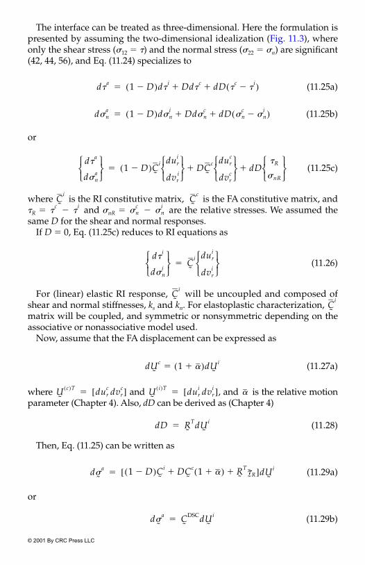
© 2001 By CRC Press LLC
The interface can be treated as three-dimensional. Here the formulation ispresented by assuming the two-dimensional idealization (Fig. 11.3), whereonly the shear stress (�12 � �) and the normal stress (�22 � �n) are significant(42, 44, 56), and Eq. (11.24) specializes to
(11.25a)
(11.25b)
or
(11.25c)
where is the RI constitutive matrix, is the FA constitutive matrix, and�R � and �nR � are the relative stresses. We assumed thesame D for the shear and normal responses.
If D � 0, Eq. (11.25c) reduces to RI equations as
(11.26)
For (linear) elastic RI response, will be uncoupled and composed ofshear and normal stiffnesses, ks and kn. For elastoplastic characterization, matrix will be coupled, and symmetric or nonsymmetric depending on theassociative or nonassociative model used.
Now, assume that the FA displacement can be expressed as
(11.27a)
where and , and is the relative motionparameter (Chapter 4). Also, dD can be derived as (Chapter 4)
(11.28)
Then, Eq. (11.25) can be written as
(11.29a)
or
(11.29b)
d�a 1 D( )d�
i Dd�c dD �
c�
i( )� ��
d�na 1 D( )d�n
i Dd�nc dD �n
c�n
i( )� ��
d�a
d�na
1 D( )C˜
i duri
dvri
DC˜
c durc
dvrc
dD�R
�nR
� ��
C˜
iC˜
c
�c
�i
�nc
�ni
d�i
d�ni
C˜
i duri
dvri
�
C˜
i
C˜
i
dU˜
c 1 ��( )� dU˜
i
U˜
c( )T durc dvr
c[ ]� U˜
i( )T duri dvr
i[ ]� �
dD R˜
TdU˜
i�
d�˜
a 1 D( )C˜
i DC˜
c 1 ��( ) R˜
T�˜R��[ ]dU
˜i
�
d�˜
a C˜
DSCdU˜
i�

© 2001 By CRC Press LLC
where and � [�R�nR]. Here matrix will be cou-pled and nonsymmetric. Analysis with Eq. (11.29) can be complex andrequire special iterative schemes. Hence, as a simplified approximation, can be assumed as zero.
11.6.1 Specializations
If the FA is assumed to carry no stress at all, as in the case of the continuumdamage model (59), and � 0 and Eq. (11.25) reduces to
(11.30)
where . Such a model is not appropriate, as it does not includethe interaction between the RI and FA parts. As a result, it would include spu-rious mesh-dependent effects (Chapter 13).
If it is assumed that the FA part can carry normal stress but no shear stresslike a constrained liquid (Chapter 4), Eq. (11.25) would reduce to
(11.31a)
or
(11.31b)
where is the constitutive matrix for the RI (elastic, elastoplastic-�0, etc.)material, and .
Now, by using Eq. (11.18), we have
(11.31c)
If the relation between and �n is linear, c2 � 1 and
(11.31d)
where c1 is the slope of the average straight line (Fig. 11.7).If the FA part is assumed to be at the critical state, , and , need
to be evaluated based on Eqs. (11.18) and (11.20). This would require an iter-ative analysis. To simplify the formulation, it can be assumed that the normal
d�˜
a( )T d�ad�n
a[ ]� �˜R
T C˜
DSC
�
C˜
c0˜
� �c
d�˜
a 1 D( )C˜
idU
˜i dD�
˜i
�
�˜
i( )T�
i�n
i[ ]�
d�a 1 D( )d�
i D 0( ) dD 0 �i
( )���
d�na 1 D( )d�n
i D d�nc dD �n
c�n
i( )� ��
d�˜
a C˜
id�
˜i Dd�
˜c dD �r� ��
Ci
d�˜
c( )T 0 d�nc[ ]� �r
T�
i �n
c �n
i[ ]�
d�c c1c2 �n
c( )c2 1( )
d�nc
��
�c
d�c c1 d�n
c�
d�c d�n
c�
c�n
c

© 2001 By CRC Press LLC
stresses are equal, i.e., . Then, using Eq. (11.31d), Eq. (11.25) can beexpressed as
(11.32)
11.6.2 Alternative DSC Equations
It can be appropriate to treat the interface zone as “solid” material with(small) finite thickness (Fig. 11.3). In that case, the formulation can beobtained by using the elastoplastic (RI) and critical-state (FA) models forinterface treated as a solid material (Chapter 7).
The stress �x (Fig. 11.3) can be assumed to be negligible, and the formu-lation can be obtained in terms of the shear stress, �, and normal stress (�n ��y) (56), with corresponding shear and normal strains, � and n, respec-tively [Eqs. (11.8) and (11.9)]. Furthermore, the disturbance, D, can beexpressed (separately) in terms of shear and normal responses as in Eqs.(11.23b and c).
Now Eq. (11.25) can be written as
(11.33)
Then and can be obtained using the critical state, Eqs. (11.18) and(11.21), as
(11.34a)
(11.34b)
where e0 is the initial void ratio of the interface material and the linear relationis assumed between and (Fig. 11.7). The equations can be simplified byassuming that , , and D � Dr � Dn:
(11.35)
When the interface zone is treated as the “solid” thin-layer element, weneed parameters relevant to the DSC/HISS models for solids. They can bedetermined from interface shear tests by using appropriate assumptions and
d�ni d�n
c�
d�a
d�na
1 D( )d�
d�ni
i
Dc1 d�n
i
d�ni
dD�R
0
���
d�a
d�na
1 Dr( )d�
i
1 Dn( )d�ni
Dr d�
c
Dn d�nc
dDr �
c�
i( )
dDn �nc
�ni
( )
� ��
d�nc d�
c
d�nc
�nc 1 e0�
--------------- dn
c�
d�c c1d�n
c�
�c
�nc
d�ni d�n
c� �n
i�n
c�
d�a
d�na
1 D( )d�
i
d�ni
Dc1 d�
i
di�n
i dD �
c�
i( )
0
���

© 2001 By CRC Press LLC
transformations, which are given below (here, the subscripts j and s denotequantities relevant to interface and solid, respectively):
Assumptions: �j � ; �nj � pj � J1s �3Elastic: for E and G, use Eq. (11.7)Plasticity: �3.0
Rs � . Rj
n from Eq. (11.37) belowa and b from Eq. (11.12), with �s � �j
Critical state: � �3.0 s from the slope of the ln e vs. ln pj plot
� void ratio, Eq. (11.21)Disturbance: Du, A, and Z, Eq. (11.22)
11.7 Determination of Parameters
The DSC model with the elastoplastic �0-version for the RI response for inter-faces involves the following constants:
The procedures for finding the above parameters are essentially similar tothat for solid materials (Chapter 7). They are described briefly below.
Elastic. The shear stiffness, ks, and normal stiffness, kn, are found as (aver-age) unloading slopes of � vs. ur and �n vs. vr curves (Fig. 11.10), respectively.If they are considered to be variable in a nonlinear elastic model, they can beexpressed as functions of factors such as � and �n.
Plasticity. The parameter � is determined from the slope of the ultimateenvelope in �–�n space [Fig. 11.11(a)]. The value of q for the curved envelopeis found from (here the superscript � is dropped for convenience)
(11.36a)
Model Constants Comment
Elastic ks, kn
Plasticity (RI) a, b, n, and � Straight ultimate envelope
a, b, n, �, and q Curved ultimateenvelope
Critical state (FA) None Zero strengthkn Normal strengthc0, c1, c2; , Critical state
Disturbance Du, A, Z If D � D� � Dn
J2D s( )
�s � j�ca
c0-----
1t---
ms mj
e0c
vr0
�u ��nq�2
�

© 2001 By CRC Press LLC
where �u is the ultimate shear stress (� � 0). The value of q is found by writingEq. (11.36a) as
(11.36b)
Then the plot of ln �u vs. ln �n provides the value of q from the slope of theaverage line [Fig. 11.11(b)]. This and subsequent figures for other parametersare relevant to test data for various joints (44), e.g., Example 11.2.
The phase or state change parameter, n, is evaluated on the basis of thestate of stress at the transition point [Fig. 11.6(b)], where the normal dis-placement is zero or changes from compression to dilation. Then, based onthe substitution of � from Eq. 11.16 in the expression for , the equa-tion for n is derived as
(11.37)
where and are the stresses at the transition point. In the case of hardmaterials, the compactive response may be very small. In that case, the
FIGURE 11.10Shear and normal stiffnesses: (a) shear, ks; (b) normal, kn.
ln �u ln �q2--- ln �n��
�F���n
nq
1 �2
��nq
----------
-------------------�
� �n

© 2001 By CRC Press LLC
hardening parameters a and b [Eq. (11.12)] and n can be found simulta-neously by first writing Eq. (11.16) as
(11.38a)
and then from Eq. (11.12a)
(11.38b)
FIGURE 11.11Determination of ultimate and critical parameters: (a) plot for �; and (b) plot for q (44, 64).
��nn
��na
�2
�� �
ln a b ln � nln �n� ln ��

© 2001 By CRC Press LLC
where � is computed at various points on the � ur and �n vr curves[Fig. 11.12(a)] for stresses (� and �n) at those points. Then Eq. (11.38b) iswritten for various points, and a least-square fit solution provides valuesof a, b, and n.
The values of a and b can also be found by writing Eq. (11.12) as
(11.39)
The values of � are computed at various points on the curves [Fig. 11.12(a)]and those of � for those points are obtained from Eq. (11.16). Then a plot ofln� vs. ln � provides values of a and b as intercept when ln � � 0, and theslope of the average curve [Fig. 11.12(b)]. The parameter b denotes rate ofhardening, and a is the value of � when � � 1, i.e., at a high value of the plasticdisplacement trajectory. The value of a is usually small and needs to be deter-mined as precisely as possible.
The critical-state parameters are found by writing Eq. (11.18) as
(11.40)
FIGURE 11.12Determination of hardening parameters.
ln a b ln � ln� �
ln �c
�0( ) ln c1 c2ln �nc
��

© 2001 By CRC Press LLC
Here, the value of c0 is obtained from a plot of vs. �n when �n � 0 (Fig. 11.7).Then the plot of ln vs. ln (�n) [Fig. 11.13(a)] provides the values of c1 and c2
as the intercept when ln �n � 0 and the slope of the average line, respectively.The parameters in Eq. (11.20) are found by writing it as
(11.41)
The plot in Fig. 11.13(b) of ln vs. �n provides values of and asintercept when �n � 0 and average slope, respectively.
The disturbance parameters (with Du � 1) are found by writing Eq. (11.23)as
(11.42)
The values of D at different points on the observed data (Fig. 11.8) arefound using corresponding curves. For example, for � ur curves, D is foundfrom
(11.42a)
FIGURE 11.13Typical plots for critical parameters for rock joint type A: (a) plot for c1 and c2; and (b) plotfor and (44). ©John Wiley & Sons Ltd. Reproduced with permission.vr
o
�c
�c( )
ln vrc ln vr
0 �n�
vrc( ) vr
0
ln ln 1 D( )[ ] ln A Z ln �D��
Dr�
i�
a
�i
�c
----------------�

© 2001 By CRC Press LLC
The values of �D are found corresponding to the points chosen. Then theplot of ln[ ln(1 Dr)] vs. ln �D (Fig. 11.14) provides the values of A and Z asthe intercept when ln �D � 0 and the average slope, respectively.
For the case of cyclic loading involving degradation [Fig. 11.8(d)], the dis-turbance can be expressed in terms of measured shear stress or effectivestress with number of cycles (N). In the case of shear stress, D can beexpressed as
(11.42b)
where is the peak shear stress at given cycles, and is the residual shearstress. Then, Eq. (11.23) is expressed in terms of �D(N), which is the deviatoricplastic displacement trajectory corresponding to peaks at given cycles. The RIshear stresses are determined based on the assumption that the continu-ation of the first cycle response, in Fig. 11.8(d), characterized using a linearelastic or elastoplastic (�0) or other model, can provide the RI response byintegrating:
(11.43)
where is the RI constitutive matrix in which the parameters are foundfrom the first cycle response. For linear elasticity, the unloading or initialslope can provide the elastic moduli. For the plasticity (�0) model, the ulti-mate parameters can be found from quasistatic tests augmented by harden-ing parameters from the initial part of the first cycle response.
For stress-controlled tests under saturated conditions in which pore waterpressures are measured under cyclic loading, D can be found based on the
FIGURE 11.14Determination of disturbance parameters (A, Z); assume Du � 1.0 (44). ©John Wiley & SonsLtd. Reproduced with permission.
D N( )�
i�
p
�i
�c
------------------�
�p
�c
�i( )
d�˜
i C˜
i dU˜
i�
C˜
i

© 2001 By CRC Press LLC
effective normal stress vs. N relation [Fig. 11.8(c)]. The RI values of`are obtained by treating the first cycle � ur response as RI. Then
(11.44a)
where is the observed stress given by
(11.44b)
where is the total normal stress and p is the measured pore water pressure.
11.7.1 Mathematical and Physical Characteristics of the DSC
In modelling interfaces and joints, it is necessary to account for the nonlocalconsideration with appropriate attention to the normal behavior. Furthermore,the microcrack interaction in the interface zone as affected by deformations ofasperities needs to be included. Also, as the material in the interface is not acontinuum and involves discontinuities due to microcracks and fractures,characteristic dimension should be a part of the model (Chapter 12). The DSCmodel allows for these factors implicitly within its framework (52–54).
Assuming that the same disturbances apply for the shear and normalbehavior, the total observed stresses, and , in the DSC are given by
(11.45a)
(11.45b)
where the disturbance is given by (Chapter 4)
(11.46)
and represents the area of distributed fully adjusted parts due to the inter-nal microstructural self-adjustment leading to microcracking and degrada-tion (of asperities). That is, the observed stresses are expressed in terms of theweighted value of the distributed FA parts in the interface zone (Fig. 11.3).Thus, the effect of the area modified by the deformations in the asperities isincluded in the description of the stresses. This approach is considered simi-lar to that in Eq. (11.3b) (11).
The incremental Eq. (11.25) includes the effect of the deformation charac-teristics of the FA (or microcracked) zones because of the existence of the sec-ond term and the first part of the third term. Note that in the continuum
�n( ) �ni( )
D N( )�n
i( )�n
a( )
�ni( )
�nc( )
------------------------�
�na( )
�na( )
�na( ) p�
�na( )
�a
�na
�a 1 D( )� i D�
c��
�na 1 D( )�n
i D�nc
��
DAc
A------�
Ac

© 2001 By CRC Press LLC
damage model, Eq. (11.30), the interaction due to the response of the dam-aged part is not included. Thus, the DSC model allows for the interactionbetween the mechanisms in the RA and FA parts. Furthermore, the third termin Eq. (11.25), which represents the relative stress , provides for interac-tive (relative) motions between the RI and FA parts.
In the description of D in Eq. (11.23), the parameters Du, A, and Z can beexpressed as functions of the size of the (test) specimen or roughness or meanparticle size of material at the interface (52–54). Also, Du is given by
(11.47)
where is the critical or unique volume (dilation) to which a given interfacezone would tend. It can be a function of (initial) normal stress or roughness (par-ticle size). In other words, Du can be considered to act as the characteristic dimen-sion. Thus, the model can allow for the characteristic dimension through Du.
11.7.2 Regularization and Penalty
The thin-layer element (Fig. 11.3) is assigned the thickness t, which can beevaluated based on analytical and�or experimental considerations (36, 56, 60).The effect of (deformation of) neighboring bodies can also be included in theformulation (56). The inclusion of thickness can be interpreted as a mathe-matical scheme to provide a penalty leading to the regularization of the uni-lateral contact (56, 61, 62). Consider the normal stress (�n) given by
(11.48)
where vr is the normal relative displacement assuming no penetration ofbody 1 into body 2 (Fig. 11.3), and n is the normal strain. If , body 2tends to “rigid” behavior. It has been shown that the thickness t acts as a pen-alty parameter and regularizes the system (62).
11.8 Testing
Laboratory or field testing are essential for the determination of parametersand calibration of constitutive models. In the context of interfaces and joints,a number of laboratory test devices have been used to measure shear andnormal responses. They include direct shear, torsion and ring shear, and
�˜ r( )
DVc
V------ tAc
tA--------��
Vc
�n Enn�
Envr
t----�
knvr�
t 0→

© 2001 By CRC Press LLC
simple shear devices; comprehensive reviews of these testing devices aregiven elsewhere (5, 42, 49).
The testing here is identified as static, quasistatic or one-way, and cyclic ortwo-way. The static test involves monotonic loading with increasing (shear)stress. The quasistatic or one-way loading involves loading–unloading andreloading cycles; however, the stress does not change sign. The cyclic or two-way case involves cycles of loading–unloading and reloading that includechange in the sign of the stress.
A brief description of the cyclic multi degree-of-freedom (CYMDOF) sheardevice (49, 63) with pore pressure measurements is given. Figure 11.15(a), (b),and (c) show an overall view, cross section, and rings for a simple shear defor-mation mode, respectively. The CYMDOF device allows testing under static,quasistatic, and cyclic load and displacement-controlled loading, dry andsaturated interfaces, direct and simple shear modes of deformation, and mea-surements of shear, normal and pore water pressure responses. It allows forthree degrees of freedom, normal, translational, and rotational. Maximumload is about 130 KN (30 Kips) and displacement amplitudes of about 2.00 cm(0.80 in) and �1.30 cm (�0.50 in.) in the vertical and horizontal directions,respectively. It can permit simulation of a wide range of interfaces (soil-struc-ture, rock joints, metal– metal, soil–geosynthetics, etc.).
11.9 Examples
The DSC and its hierarchical (elastic, nonlinear elastic, d0-plasticity, etc.) ver-sions have been used to characterize a wide range of dry and fluid saturatedinterfaces and joints under static, quasistatic, and cyclic loading. Table 11.1shows details of these applications.
TABLE 11.1
Review of Interface/Joint Models
Model and Details References
Nonlinear elastic models for shear and normal response under quasistatic or one-way loading for dry interfaces
3, 5, 28, 30, 36, 37, 38, 39, 41
Elastoplastic (�0��1) models under quasistatic loading for dry interfaces and joints
42, 43, 44, 45, 46, 74, 75
DSC and elastoplastic models under quasistatic and cyclic loading for dry interfaces
43, 44, 46, 51, 69, 70
DSC and elastoplastic models under quasistatic and cycling loading for saturated interfaces
49, 50
Viscoplastic model under quasistatic loading for dry and wet interfaces
47, 48
DSC model for thermomechanical behavior of joints (Pb�Snsolders) under cyclic loading
77–79

© 2001 By CRC Press LLC
It is found that for more realistic simulation of interface behavior, in gen-eral, it is necessary to include factors such as irreversible deformations,microcracking, and degradation at interfaces in addition to the elasticresponse. Hence, in the upcoming examples, major attention is given to the
FIGURE 11.15Details of CYMDOF-P device: (a) overall view; (b) cross section of specimen; and (c) ringsfor simple shear mode (49, 63, 73).

© 2001 By CRC Press LLC
DSC and its specialized versions such as �0-associative plasticity models inthe HISS approach.
Example 11.1 Concrete–Concrete InterfaceFigure 11.16(a) shows a schematic of interface or joint between concrete withdifferent teeth angles � (� 5, 7, 9 degrees) that were tested using the CYM-DOF device under different normal stresses (42, 55). The parameters for theDSC model for � � 5� and 9� (Table 11.2) were obtained as average valuesfrom tests with � � 5� and 9� (44, 64). Figure 11.16(b) and (c) show compari-sons between back predictions and observed test results for � � 7�. This is anindependent validation, as it was not used for finding the average constants(Table 11.2).
Example 11.2 Rock JointsSchneider (57, 58) reported a series of shear tests on rock joints, Type C, A,and B, indicating smooth to rough conditions. Type C was joint in a limestoneand is considered to be smooth; Type A was joint in a granite and is consid-ered to be medium-rough; and Type B was a joint in sandstone, which wasrougher. Table 11.3 shows material parameters for the three joint types.
Figure 11.17 shows comparisons between the � ur and vr vs. ur relationsfor the three joint types from smooth (C) to intermediate (A) to rough (B)joints. The vr vs. ur plots are shown only for typical values of �n � 0.61, 1.38,and 1.29 MPa, respectively.
Bandis et al. (65) reported shear tests for simulated rock joints with differentnormal stresses and roughness defined by JRC (joint roughness coefficient).
TABLE 11.2
Constants for Back Predictions. Concrete–Concrete Interface (a) � � 5�; and (b) � � 9� (64)
� � 5� � � 9�
Elastic constants kn 6.2 MPa �mm 6.2 MPa �mmks 31.0 MPa �mm 31.0 MPa �mm
Yield function F a 0.0035 0.0085b 0.9 0.9n 2.1 2.1� 0.0936 0.303q 1.79 1.98
Critical state c1 0.48 0.81c2 0.895 0.99
0.81 0.810.0 0.0
Disturbed state A� 1.15 3.29Eq. (11.23) Z� 0.37 0.65
An 0.85 0.85Zn 1.85 1.85
vro

© 2001 By CRC Press LLC
Details of the DSC modelling and validation for these test data are given else-where (44, 64).
Example 11.3 Rock–Pile InterfaceWilliams (66) reported laboratory direct shear tests on interface between pileand a weak rock. In contrast to the foregoing tests where the normal stresswas kept constant, the normal stiffness (kn) was kept constant. The normalstiffness was directly proportional to the normal displacement (dilation). Thetests were performed under different (constant) normal stiffnesses and initialnormal stress, . The material parameters for the DSC model were determinedusing a number of tests. Their average values (Table 11.4) were used to per-form independent back prediction as described ahead.
Figure 11.18 shows comparisons between back predictions and observa-tions in terms of � vs. ur , vr vs. ur , �n vs. ur , and � vs. �n for � 15.0 kPa and
FIGURE 11.16Comparisons of predictions and observations for concrete–concrete interface, teeth angle �7�; (a) � vs. ur , (b) vr vs. ur (44, 64). ©John Wiley & Sons Ltd. Reproduced with permission.
�n0
�n0

© 2001 By CRC Press LLC
kn � 36.0 kPa/mm. This test was not used for finding the parameters (Table 11.4);hence, it is an independent validation.
The constant normal stiffness test is relatively complex and exhibits differ-ent behavior compared to the constant normal stress tests. Here, the normalstress increases [Fig. 11.18(d)], and the mobilized friction angle �m (tan �m ����n) decreases and tends to the residual value. This is because, as the shearstress increases, the normal stress increases faster, and the ratio ���n decreaseswith shearing. This phenomenon, before the peak stress, is termed as weaken-ing in contrast to softening. In the case of the latter, the shear stress after the
TABLE 11.3
Constants for Back Predictions. Rock Joints: (a) Type C — Smooth, (b) Type A — Medium Rough, and Type B — Rough (64)
Type C Type A Type B
Elastic constants kn 4.2 MPa �mm 5.6 MPa �mm 5.0 MPa �mmks 21.0 MPa �mm 28.0 MPa �mm 25.0 MPa �mm
Yield function F a 0.0082 0.0656 0.124b 1.05 1.42 1.21n 2.10 2.31 2.23� 1.91 3.24 3.68q 1.98 1.91 1.97
Critical state c1 0.82 0.90 0.89c2 0.99 0.955 0.985
3.80 4.94 7.520.873 1.21 1.069
Disturbed state A� 2.97 3.87 6.27Z� 0.30 0.36 0.90An 4.18 3.88 7.99Zn 1.64 0.90 1.52
TABLE 11.4
Constants for Back Predictions. Rock-Pile Interface: Test SM4 (64)
Elastic constants kn 1.0 MPa/mmks 5.0 MPa/mm
Yield function F a 0.1b 4.5n 3.0� 42.5q 1.78
Critical state c1 1.27c2 0.89
2.110.0
Disturbed state A� 5.16Z� 0.96An 5.23Zn 1.19
vro
vr0

© 2001 By CRC Press LLC
peak drops. In contrast, in the constant normal stress tests, �m increases up tothe peak and then decreases.
Example 11.4 Dry Sand–Concrete Interfaces: Static and Cyclic BehaviorA series of laboratory tests using a simple shear device have been reported byUesugi et al. (67, 68) for sand (Toyoura)–concrete and sand–steel interfaces.
FIGURE 11.17Comparisons of predictions and observations for rock joints: (a) � vs. ur, type C joint; (b) vr
vs. ur, type C joint; (c) � vs. ur, type A joint; (d) vr vs. ur, type A joint; (e) � vs. ur, type B joint;(f) vr vs. ur, type B joint (44, 64).

© 2001 By CRC Press LLC
The tests were performed under different surface roughness (R), initial normalstress (�n), and relative density (Dr). Details of the DSC model and associatedplasticity (RI) model are given in (43). Here the effect of roughness of the inter-face was included in the ultimate parameters and disturbance parameters forthe static and cyclic tests. The roughness was defined as (43, 67, 68)
(11.49a)
FIGURE 11.17(continued)
RRn
RnCr
-------- if RnCr Rn��
R 1 if RnCr Rn��

© 2001 By CRC Press LLC
where Rn is the normalized roughness:
(11.49b)
Rmax is the relative height between the highest peak and lowest trough alonga surface (asperity) profile over the length L, which can be adopted depend-ing on roughness, e.g., L � D50 or 0.2 mm, D50 is the mean diameter of sandparticles, and is the critical normalized roughness beyond which theshear failure would occur in soil rather than at the interface.
The effect of roughness (R) on the hardening and disturbance behavior wasincorporated by expressing various quantities in terms of R. The hardeningfunction, �, in Eq. (11.11) was expressed as
(11.50a)
(11.50b)
FIGURE 11.18Comparisons of predictions and observations for rock–pile interface, independent test: �15 kPa, kn � 36.0 kPa�mm; (a) � vs. ur; (b) vr vs. ur; (c) �n vs. ur; (d) � vs. �n (44, 64).
�n0
Rn
Rmax L( )D50
-------------------�
RnCr
� � �1�v( )�D
� �D
�D�
--------------------
b1
for �D �D� �exp�
� 0 for �D � �D� �

© 2001 By CRC Press LLC
where is the value of �D at the peak shear stress, �p, and a1 and b1 are hard-ening parameters. For the nonassociative �1 model, the hardening function,�Q (Eq. 11.57b below), was expressed as
(11.51a)
where is the value of � at the phase change point, � is the nonassociativeparameter, and
(11.51b)
(11.51c)
The ratios �p ��n, �r ��n, and were expressed as functions of R:
(11.52a)
FIGURE 11.18(continued)
�D�
�Q � �ph 1��i----
1 � 1DDu------
��
�ph
D 0 for �D �D� ��
D Du 1 A �D �D� ( )
2( )exp[ ] for �D �D
� ��
�D�
�p ��p
�n----- 1
R---- �p1 �p2R�( )� � �

© 2001 By CRC Press LLC
(11.52b)
(11.52c)
where �p1, �p2, �01, �02, , and are material parameters, �r is the residualshear stress, and denotes the roundness of sand particles. Equations(11.52a and b) are used in Eq. (11.50), and Eq. (11.52c) introduces the effect ofR on the disturbance through Du in Eq. (11.51c).
The DSC parameters were found from tests reported in (67, 68); their valuesare given in (43).
Figure 11.19 shows comparisons between back predictions and static testdata for different roughness for �n � 98 kPa and Dr � 90%, for concrete–Toy-oura sand interface.
Figure 11.20 shows comparisons for cyclic tests for �n � 98 kPa, Dr � 90%,and Rmax � 23 �m, in terms of ���n vs. ur and vr vs. ur , with number cycles(N � 1, 2, , 15).
Example 11.5 Dry Sand-Steel Interfaces: Static Two- and Three-Dimensional BehaviorFakharian and Evgin (69) used the DSC with HISS �1-plasticity model for the RIbehavior and constrained-liquid simulation for the FA response, i.e., the
FIGURE 11.19Comparisons for dry sand (Toyoura)–concrete interface, static loading: �n � 98 kPa, Dr �
90% (43).
�0
�r
�n----- 1
R---- �01 �02R�( )� �
�D� �D1
� �D2� R�( )�
�D1� �D2
�
R
…

© 2001 By CRC Press LLC
material parts in the FA state cannot carry shear stress. They calibrated themodel on the basis of laboratory tests for interfaces between a medium silicasand with relative density, Dr � 88%, and steel (plate) by using the test devicedescribed in (70). The sand-blasting technique was used to obtain differentsurface roughnesses, Rmax (Eq. 11.49b) � 4, 15, and 25 �m, which cover therange from smooth to rough conditions.
The DSC model used was the same as in Example 11.4. The materialparameters were found from a series of two-dimensional laboratory testsdepicted in Fig. 11.21; details of parameters and the test device are given in(69, 70).
Figure 11.22 shows comparisons between back predictions and test datafor the two-dimensional test in which the shear displacement was appliedwith constant normal stress �n � 100 kPa and sand density Dr � 88%. Thecomparisons involve Rmax � 3.6 and 25 �m, while the results for Rmax � 15 �m
FIGURE 11.20Comparisons for sand (Toyoura)–steel interface, cyclic loading: �n � 98 kPa, Dr � 90%, Rmax �
23 �m (43).
FIGURE 11.21Stresses acting on an interface: (a) 3-D, (b) 2-D (69). ©John Wiley & Sons Ltd. Reproducedwith permission.

© 2001 By CRC Press LLC
involved only predictions. It can be seen that the model provides satisfac-tory predictions of hardening, dilative, peak, and softening responses. Forthe case of the smooth interface (Rmax � 3.6 �m), the predictions showessentially zero normal displacement, while the test data show nonzerocompression.
For the three-dimensional case, the yield function [Eq. (11.11)] was modi-fied as (69)
(11.53)
In the three-dimensional tests, the shear stress �y � 0, 20, 40, and 60 kPawas applied with �n � 100 kPa (Fig. 11.21). Then the interface was sheared inthe x-direction by increasing �x with constant values of �y and �n. The stressand displacement paths followed in the tests are shown in Fig. 11.23.
Figure 11.24 shows comparisons between the predictions and test data forshear stress, �x, versus shear displacement, ux, and normal displacement, v,versus ux for the three-dimensional tests. Figure 11.23 shows comparisonsbetween the predicted and observed stress paths. The parameters from the two-dimensional tests were used for the three-dimensional analysis; hence, this isconsidered to be an independent prediction. Overall, the predictions comparewell with the observed behavior, particularly because this is an independentvalidation. Details of tests and validations for tests under constant stiffness con-dition (Example 11.3) are also reported by Fakharian and Evgin (69).
FIGURE 11.22Comparisons between predictions and test data for 2-D tests: �n � 100 kPa, Dr � 88%. ForRmax � 15, only predictions are shown (69). ©John Wiley & Sons Ltd. Reproduced withpermission.
F �x2
�y2
��nn
��n2
� � 0� �

© 2001 By CRC Press LLC
Example 11.6 Soil–Rock Interface: Viscoplastic ModelA smeared interface zone occurs between the moving mass of soil and bedrock in the case of creeping slopes and landslides (47, 48); Fig. 11.25(a) showsa schematic of such an interface. The mechanical behavior of the interfacezone can involve creep or viscous deformations in addition to elastic andplastic deformations.
A viscoplastic model for the interface zone has been developed, verified,and used (47, 48) to characterize the interface zone at the site of the Villar-beney landslide in Switzerland (71). Brief details of the model are givenahead.
The incremental elastoplastic equations for the HISS (�0 ��1) models can bewritten as
(11.54a)
where d � [d� d�n], d � [dur dvr], and is the elastoplastic matrixderived using the yield function, F [Eq. (11.11)], in the context of consistencycondition, dF � 0, and the normality rule
FIGURE 11.23Comparisons between predictions and test data for stress and displacement paths for 3-Dtests: �n � 100 kPa (69). ©John Wiley & Sons Ltd. Reproduced with permission.
d�˜
C˜
epdU
˜�
�˜
T U˜
C˜
ep

© 2001 By CRC Press LLC
FIGURE 11.24Comparisons between predictions and test data for different values of �y in 3-D tests: �n �
100 kPa, Rmax � 25 �m, Dr � 88% (69). ©John Wiley & Sons Ltd. Reproduced with permission.
FIGURE 11.25(a) Schematic of interface in creeping slope; (b) cross section of interface test specimen(47, 48). ©John Wiley & Sons Ltd. Reproduced with permission.

© 2001 By CRC Press LLC
(11.54b)
where , is the scalar proportionality factor, and Q isthe plastic potential function. In the case of associative plasticity, Q F(Chapter 7).
Perzyna’s (72) theory of viscoplasticity is used to characterize the predom-inant plastic deformations, i.e., the viscoelastic component is assumed to besmall. Accordingly, the viscoplastic strain rate is given by (see Chapter 8)
(11.55a)
or
(11.55b)
where Q is the scalar flow (plastic potential) function, � is the fluidity param-eter, F0 is the normalizing constant (e.g., yield stress, atmospheric pressure),and the angle bracket has the following meaning:
(11.56)
Nonassociative Response. For nonassociative behavior, the plastic poten-tial function, Q, is written as
(11.57a)
and the hardening function, �Q, is given by
(11.57b)
where �0 is the value of � at the initiation of the nonassociative response, rv isthe ratio of the plastic normal displacement trajectory (�v) to the total trajec-tory, � [Eq. (11.13)], and � is the nonassociative parameter (Chapter 7). For thecase of smooth interfaces, dilation is not significant, and the followingexpression can be used for �Q:
(11.58)
dU˜
p
�Q��
˜
--------�
dU˜
p( )T durp dvr
p[ ]��
˜
vp� �
FF0-----
�Q��
˜
--------���
� �� FF0-----�
�Q��--------
�Q��n-------------------
�
⟨ ⟩
� F�F0( )� F�F0( ) if F�F0 0�
0 if F�F0 � 0
�
Q �2
�Q�n�n
�n�2
��
�Q � � �0 �( ) 1 rv( )��
�Q � �ph 1��0-----
�
��

© 2001 By CRC Press LLC
where �ph � (2�n)� and �0 � � are the values of � (in Eq. 11.11) atthe transition point (Fig. 11.6) and at the start of the shear loading (i.e., at theend of the normal loading), respectively, and � is the nonassociative parame-ter. The hardening function � in Eq. (11.11) used here is given by
(11.59)
where and are the trajectories of volumetric and deviatoric viscoplasticstrains (displacements), respectively, and a and b are hardening parameters.
11.9.1 Creep Behavior
The parameters � and � define the viscous or creep response. The latter isgiven by
(11.60)
where N is the material parameter.
11.9.2 Testing
A series of laboratory tests were performed by using the CYMDOF, triaxial,and direct shear devices (47, 48, 71). They include both quasistatic or one-way(loading–unloading–reloading) and creep tests. The drained tests using theCYMDOF device involved interface simulation [Fig. 11.25(b)] and were con-ducted under different normal stresses, �n � 103, 207, and 345 kPa, with dif-ferent amplitudes of shear displacements, � 0.19, 0.64, and 1.27 cm. Theparameters for the viscoplastic model are shown in Table 11.5.
Figures 11.26 and 11.27 show comparisons between back predictions andobservations for a typical static test and for the creep tests, respectively.
Example 11.7 Saturated Clay–Steel Interfaces: Cyclic BehaviorThe CYMDOF-P device (Fig. 11.15) was used to perform a number ofcyclic undrained (two-way) tests for saturated marine clay–steel inter-faces, under different normal stresses and amplitudes of displacements(49, 73). The DSC constitutive model was formulated based on the elasto-plastic (�0) model to characterize the RI response, the critical state for theFA response, and the disturbance was found based on cyclic degradationdata [Fig. 11.28(a)].
�n2n
�n2n
��e
a�vvp
1 � Dvp
�( )b------------------------�
�vvp
�Dvp
�FF0-----
FF0-----
�N
ura

© 2001 By CRC Press LLC
TABLE 11.5
Parameters for Interface Model in Creeping Slope (47, 48)
Parameters Symbol Value
Elastic
Normal stiffness kn 8 � kPa�cmShear stiffness ks 2800 kPa/cm
Plastic
Ultimate � 0.24Transition n 2.04Hardening a 143.0Hardening b 10.0Nonassociative � 0.57
Viscous
Fluidity � 0.057/minExponent N 3.15
FIGURE 11.26Comparisons between predictions and observations for interface test at �n � 103 kPa (47, 48).
FIGURE 11.27Comparisons between prediction and observation for creep tests, stress ratio � 0.6: (a)preconsolidation stress � 200 kPa; (b) preconsolidation stress � 400 kPa (47, 48).
106
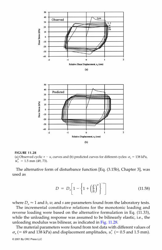
© 2001 By CRC Press LLC
The alternative form of disturbance function [Eq. (3.15b), Chapter 3], wasused as
(11.58)
where Du � 1 and h, w, and s are parameters found from the laboratory tests.The incremental constitutive relations for the monotonic loading and
reverse loading were based on the alternative formulation in Eq. (11.33),while the unloading response was assumed to be bilinearly elastic, i.e., theunloading modulus was bilinear, as indicated in Fig. 11.28.
The material parameters were found from test data with different values of�n (� 69 and 138 kPa) and displacement amplitudes, (� 0.5 and 1.5 mm).
FIGURE 11.28(a) Observed cyclic � ur curves and (b) predicted curves for different cycles: �n � 138 kPa,
� 1.5 mm (49, 73).ura
D Du 1 1 �h---
w
�
s
�
ura

© 2001 By CRC Press LLC
Typical parameters for the test with �n � 138 kPa and � 1.5 mm are shownin Table 11.6.
Figures 11.28 and 11.29 show typical comparisons between predictedresults and observed data in terms of � vs. ur and pore water pressure vs. time(cycles) for the test with �n � 138 kPa and � 1.5 mm.
Sand–Steel Interfaces: Quasistatic and Cyclic Behavior. A series oflaboratory tests were performed for dry and (partially) saturated sand(Ottawa)–steel interfaces by using the CYMDOF-P device (50). The testswere performed under different normal stresses, �n (69, 138, 207 kPa),amplitudes of displacements, (3.5, 4.3, 1.27 mm) and rates of loading(1.27, 2.54, 36.58 mm�min). Calibration of the DSC model and its validationare given in (50).
Example 11.8 Sand–Geosynthetic Interfaces: Static ResponseLaboratory static direct tests were performed (51) to measure the interfaceresponse between a sand and geogrid (geosynthetic reinforcement) underdifferent normal stresses, �n (26.8, 53.6, 80.4, and 214.4 kPa).
The DSC model was formulated based on the test data with Eq. (11.32). TheRI behavior was assumed to be elastoplastic (�0-model), and the FA responsewas simulated using the critical state. Table 11.7 shows the material parame-
TABLE 11.6
Parameters for Cyclic Test, Clay–Steel Interface, for � 1.5 mm (73)
Parameters Average�n � 69
kPa�n � 138
kPa�n � 207
kPa
Intact StateElastic E 4,400 2,400 4,300 6,500
� 0.42 0.41 0.42 0.42Plastic n 2.1 2.1 2.1 2.1
3.622 2.822 2.88 5.222a 2.63 2.701 2.586 2.601b 0.067 0.024 0.087 0.09
Critical State 0.37 0.408 0.356 0.346 0.298 0.298 0.298 0.298
1.359 1.359 1.359 1.359e0 1.69 1.49 1.37
Disturbance FunctionShear h� 3.76 4.153 9.411 0.156Eq. (11.58) w� 0.64 0.916 0.498 1.035
s� 2 2 2 2Normal hn 8.941 17.62 10.62 0.791
Eq. (11.58) wn 0.745 0.825 0.766 0.703sn 2 2 2 2
ura
�
m
e0c
ura
ura
ura
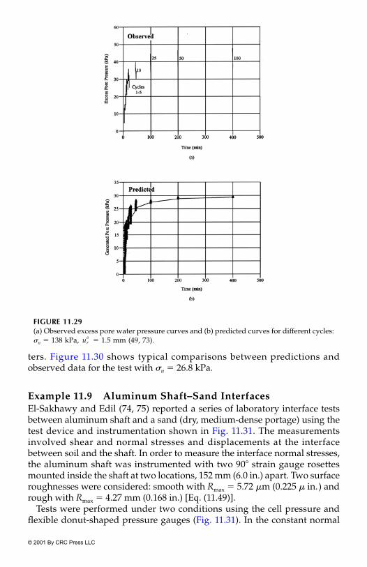
© 2001 By CRC Press LLC
ters. Figure 11.30 shows typical comparisons between predictions andobserved data for the test with �n � 26.8 kPa.
Example 11.9 Aluminum Shaft–Sand InterfacesEl-Sakhawy and Edil (74, 75) reported a series of laboratory interface testsbetween aluminum shaft and a sand (dry, medium-dense portage) using thetest device and instrumentation shown in Fig. 11.31. The measurementsinvolved shear and normal stresses and displacements at the interfacebetween soil and the shaft. In order to measure the interface normal stresses,the aluminum shaft was instrumented with two 90� strain gauge rosettesmounted inside the shaft at two locations, 152 mm (6.0 in.) apart. Two surfaceroughnesses were considered: smooth with Rmax � 5.72 �m (0.225 � in.) andrough with Rmax � 4.27 mm (0.168 in.) [Eq. (11.49)].
Tests were performed under two conditions using the cell pressure andflexible donut-shaped pressure gauges (Fig. 11.31). In the constant normal
FIGURE 11.29(a) Observed excess pore water pressure curves and (b) predicted curves for different cycles:�n � 138 kPa, � 1.5 mm (49, 73).ur
a

© 2001 By CRC Press LLC
stress tests, independent cell fluid and flexible-top boundary bag pressuresprovided constant horizontal (radial) and vertical normal stresses. In the con-stant volume test, the cell fluid and the fluid in the flexible-top boundary bagwere sealed after the application of the initial horizontal and vertical normalstresses (75).
The interface model based on HISS �1-plasticity model (42, 47) [Eq. (11.57)]was used to characterize the behavior of interfaces. The parameters obtainedfrom the test data are shown in Table 11.8 (74); they were found from testsunder three normal stresses: �n � 34.5, 69.0, and 103.5 kPa.
TABLE 11.7
Material Constants for Geosythetic Interface (51)
Elastic parameters kn 550 kPa/mmks 88.83 kPa/mm
Intact state � 95.7n 1.4q 1.395a1 96.9324�1 0.01965
Critical state c1 0.4560.2635
0.0444Disturbance A� 0.0896
Z� 2.2935An 1.1158Zn 1.17Du 0.90
Note: The parameters are obtained from nondimension-alized quantities, with respect to pa.
©John Wiley & Sons Ltd. Reproduced with permission.
FIGURE 11.30(a) Observed and predicted � vs. ur and (b) vr vs. ur curves, one-way loading for sand–geo-synthetic interface: �n � 26.8 kPa (51). ©John Wiley & Sons Ltd. Reproduced with permission.
vr0

© 2001 By CRC Press LLC
Figure 11.32(a and b) show comparisons between the laboratory sheartests and nonassociative model predictions for the smooth and roughinterfaces, respectively, under constant stress tests. It can be seen that thecorrelations are very good. It was reported (75) that the predictions fornormal displacements showed consistent trends but did not provide asgood correlations.
Example 11.10 Solder Joint in Electronic Chip-Substrate Systems: Thermomechanical BehaviorIn electronic packaging and semiconductor systems (76) (Fig. 11.33), the joiningmaterials, e.g., solders (Pb�Sn) whose thickness is small, of the order 200 �m,can be treated as bulk interface zones with thickness t. Development and
TABLE 11.8
Parameters for Shaft–Sand Interfaces (75)
ParameterSmoothinterface
Roughinterface
Elastic ks 460 kPa �mm 1600 kPa �mmkn 5400 kPa �mm 5400 kPa �mm
Plastic (average) � 0.246 1.25n 2.05 2.13a 0.0096 0.088b 0.517 0.415� 1.124 —� — 1.120
FIGURE 11.31Instrumented shaft and sand (75).

© 2001 By CRC Press LLC
application of the DSC model with �0-plasticity model for the RI response forsolders are given in Chapter 7. Development, validations, and computerpredictions for various chip-substrate systems are given in (77–79) and inChapter 13.
Example 11.11 Homework ProblemsDerive the matrix in Eq. (11.25) by assuming that the RI behavior is sim-ulated as linear elastic with ks and kn, and as elastoplastic with F in Eq. (11.11).Then by assuming that the strains (displacements) in the RI and FA parts areequal, derive the special form of Eq. (11.25). Further, assume that the FAbehavior is simulated such that it cannot carry any stress at all, i.e., inEq. (11.22a) is zero. Then by using the parameters in Table 11.2, backpredictthe responses for � � 0.138 MPa (Fig. 11.16).
Hint: You may prepare a computer routine for the integration of the special-ized form of Eq. (11.25). The predictions you obtain may not be the same as
FIGURE 11.32Comparison between model predictions and test behavior for constant stress tests (75).
FIGURE 11.33Leadless ceramic chip carrier (LCCC) (76).
C˜
i
�c

© 2001 By CRC Press LLC
in Fig. 11.16 because the FA response is characterized using the critical-stateequations. This problem is designed mainly to illustrate the procedureinvolved in back predictions.
11.10 Computer Implementation
Details of the implementation of the DSC models are given in Chapter 13. Thethin-layer interface�joint element is formulated in the same manner as thesolid (two- or three-dimensional) element. The stiffness matrix for the inter-face element usually has the same number of degrees of freedom as the solidelement; hence, it is assembled directly with the solid elements.
References
1. Bowden, F.P. and Tabor, D., The Friction and Lubrication of Solids, Part I, Claren-don Press, Oxford, 1950.
2. Rabinowicz, E., Friction and Wear of Materials, John Wiley, New York, 1965. 3. Desai, C.S. and Christian, J.T. (Eds.), Numerical Methods in Geotechnical Engi-
neering, McGraw-Hill, New York, 1977. 4. Dawson, D., The History of Tribology, Longman, London, 1978. 5. Desai, C.S., “Behavior of Interfaces Between Structural and Geologic Media,”
A state-of-the-art paper, Proc., Int. Conf. on Recent Advances in Geotech. EarthquakeEng. and Soil Dynamics, St. Louis, MO, 1981.
6. Kikuchi, N. and Oden, J.T., Contact Problems in Elasticity, Siam, Philadelphia,1981.
7. Suh, N.P. and Sih, H.C., “The Genesis of Friction,” Wear, 69, 1981, 91–114. 8. Madakson, P.B., “The Frictional Behavior of Materials,” Wear, 87, 1983, 191–206. 9. Amontons, G., “De La Resistance Causee les Machines,” Memories de l’Academie
Royale, A. Chez Gerard Kuyper, Amsterdam, 1699, 257–282.10. Archard, J.I., “Elastic Deformation and the Laws of Friction,” Proc., Roy. Soc.,
London, Series A, Vol. 243, 1959, 190–205.11. Oden, J.T. and Pires, T.B., “Nonlocal and Nonlinear Friction Laws and Varia-
tional Principles for Contact Problems in Elasticity,” J. of Appl. Mech., Vol. 50,1983, 67–75.
12. Tolstoi, D.M., “Significance of Normal Degree-of-Freedom and Natural NormalVibrations in Contact Friction,” Wear, 10, 1967, 199–213.
13. Seguchi, Y., Shindo, A., Tomita, Y., and Sunohara, M., “Sliding Rule of Frictionin Plastic Forming Metal,” Computational Methods in Nonlinear Mechanics (Oden,J.T., et al., Editors), The Univ. of Texas, Austin, 1974, 683–692.
14. Fredriksson, B., “Finite Element Solution of Surface Nonlinearities in StructuralMechanics with Special Emphasis to Contact and Fracture Problems,” Computerand Structures, Vol. 6, 1976, 281–290.
15. Herrmann, L.R., “Finite Element Analysis of Contact Problems,” J. of Eng. Mech.,ASCE, 104, 1978, 1043–1057.

© 2001 By CRC Press LLC
16. Michalowski, R. and Mroz, Z., “Associated and Non-associated Sliding Rulesin Contact-Friction Problems,” Arch. Mech., 30, 1978, 259–276.
17. Kikuchi, N. and Song, Y.S., “Penalty�Finite-Element Approximations of a Classof Unilateral Problems in Linear Elasticity,” Appl. Math., XXXIX, 1981, 1–22.
18. Cheng, J.H. and Kikuchi, N., “An Incremental Constitutive Relation of Unilat-eral Contact Friction for Large Deformation Analysis,” J. of Appl. Mech., ASMETrans. Paper No. 85-APM-24, 1985.
19. Jaeger, J.C., “The Frictional Properties of Joints in Rock,” Pure Appl. Geophys.,43, 1959, 148–158.
20. Patton, F.D., “Multiple Modelling of Shear Failure in Rock,” Proc., 1st Cong.Rock Mech., Lisbon, 1, 1966, 509–513.
21. Goodman, R.E., Taylor, R.L., and Brekke, T.L., “A Model for the Mechanics ofJointed Rock,” J. of Soil Mech. & Found. Eng., ASCE, 94, 1968, 637–659.
22. Zienkiewicz, O.C., Best, B., Dullage, C., and Stag, K.G., “Analysis of NonlinearProblems in Rock Mechanics with Particular Reference to Jointed Rock Sys-tems,” Proc., 2nd Int. Conf. of Rock Mechanics, Belgrade, Yugoslavia, 3, 1970,501–509.
23. Ladanyi, B. and Archmbault, G., “Simulation of Shear Behavior of a JointedRock Mass,” Proc., 11th O.S. Symp. Rock Mech., Berkeley, CA, 1970, 105–125.
24. Isenberg, J., Lee, L., and Agbabian, M.S., “Response of Structures to CombinedBlast Effects,” J. Transp. Eng., ASCE, 99, 1973, 887–908.
25. Ghaboussi, J., Wilson, E.L. and Isenberg, J., “Finite Element for Rock Joints andInterfaces,” J. of Soil Mech. and Found. Eng., ASCE, 99, 1973, 833–848.
26. Barton, N.R., “A Review of a New Shear Strength Criterion for Rock Joints,”Eng. Geology, 7, 1973, 287–332.
27. Hsu-Jun, K., “Nonlinear Analysis of the Mechanical Properties of Joint andWeak Interaction in Rock,” Proc., 3rd Int. Conf. Num. Meth. in Geomech., Aachen,W. Germany, 1973, 523–532.
28. Desai, C.S., “Numerical Design-Analysis of Piles in Sands,” J. Geotech. Eng.,ASCE, 100, 1974, 613–625.
29. Kausel, E., Roesset, J.M., and Christian, J.T., “Nonlinear Behavior in Soil-Struc-ture Interaction,” J. of Geotech. Eng., ASCE, 102, 12, 1976.
30. Desai, C.S., “Soil-Structure Interaction and Simulation Problems,” Chap. 7 inFinite Elements in Geomechanics, G. Gudehus (Editor), Wiley, Chichester, U.K.,1977.
31. Wolf, J.P., “Seismic Response Due to Travelling Wave Including Soil-StructureInteraction with Base Mat Uplift,” Earthquake Eng. & Struct. Dyn., 5, 1977,337–363.
32. Lightner, J.G. and Desai, C.S., “Improved Numerical Procedures for Soil-Struc-ture Interaction Including Simulation of Construction Sequences,” Report No.VPI-E-79-32, Dept. of Civil Eng., Virginia Tech., Blacksburg, VA, 1979.
33. Toki, K.T., Sato, T., and Muira, F., “Separation and Sliding Between Soil andStructure During Strong Ground Motion,” Earthquake Eng. & Struct. Dyn., 9,1981, 263–277.
34. Katona, M.G., “A Simple Contact-Friction Interface Element with Applicationsto Buried Culverts,” Int. J. Num. Analyt. Methods in Geomech., 7, 3, 1983, 371–384.
35. Vaughan, D.K. and Isenberg, J., “Nonlinear Rocking Response of Model Con-tainment Structures,” Earthquake Eng. & Struct. Dyn., 11, 1983, 275–296.

© 2001 By CRC Press LLC
36. Desai, C.S., Zaman, M.M., Lightner, J.G., and Siriwardane, H.J., “Thin-LayerElement for Interfaces and Joints,” Int. J. Num. Analyt. Meth. in Geomech., 8, 1,1984, 19–43.
37. Zaman, M.M., Desai, C.S., and Drumm, E.C., “An Interface Model for DynamicSoil Structure Interaction,” J. Geotech. Eng. Div., ASCE, 110, 9, 1984, 1257–1273.
38. Drumm, E.C. and Desai, C.S., “Determination of Parameters for a Model forCyclic Behavior of Interfaces,” J. of Earthquake Eng. & Struct. Dynamics, 14, 1,1986, 1–18.
39. Desai, C.S., Drumm, E.C., and Zaman, M.M., “Cyclic Testing and Modellingof Interfaces,” J. Geotech. Eng., ASCE, 111, 6, 1985, 793–815.
40. Plesha, M.E., “Constitutive Models for Rock Discontinuities with Dilatancy andSurface Degradation,” Int. J. Num. Analyt. Methods in Geomech., 11, 1987, 345-362.
41. Desai, C.S. and Nagaraj, B.K., “Modeling for Cyclic Normal and Shear Behaviorof Interfaces,” J. Eng. Mech., ASCE, 114, 1988, 1198–1217.
42. Desai, C.S. and Fishman, K.L., “Plasticity Based Constitutive Model with As-sociated Testing for Joints,” Int. J. Rock Mech. & Min. Sc., 4, 28, 1991, 15–26.
43. Navayogarajah, N., Desai, C.S., and Kiousis, P.D., “Hierarchical Single SurfaceModel for Static and Cyclic Behavior of Interfaces,” J. of Eng. Mech., ASCE, 118,5, 1992, 990–1011.
44. Desai, C.S. and Ma, Y., “Modelling of Joints and Interfaces Using the DisturbedState Concept,” Int. J. Num. Analyt. Meth. Geomech., 16, 1992, 623–653.
45. Desai, C.S., “Hierarchical Single Surface and the Disturbed State ConstitutiveModels with Emphasis on Geotechnical Applications,” Chap. 5 in GeotechnicalEngineering, K.R. Saxena (Editor), Oxford & IBM Publishing Co., New Delhi,India, 1994.
46. Desai, C.S., “Constitutive Modelling Using the Disturbed State as Microstruc-ture Self-Adjustment,” Chap. 8 in Continuum Models for Materials with Micro-structures, H.B. Mühlhaus (Editor), John Wiley, Chichester, U.K., 1995.
47. Desai, C.S., Samtani, N.C., and Vulliet, L., “Constitutive Modelling and Anal-ysis of Creeping Slopes,” J. Geotech. Eng., ASCE, 121, 1, 1995, 43–56.
48. Samtani, N.C., Desai, C.S., and Vulliet, L., “An Interface Model to DescribeViscoplastic Behavior,” Int. J. Num. Analty. Meth. Geomech., 20, 1996, 231–252.
49. Desai, C.S. and Rigby, D.B., “Cyclic Interface and Joint Shear Device IncludingPore Pressure Effects,” J. of Geotech. & Geoenv. Eng., ASCE, 123, 6, 1997, 568–579.
50. Alanazy, A. and Desai, C.S., “Testing and Modelling of Sand-Steel InterfacesUnder Static and Cyclic Loading,” Report, Dept. of Civil Engng. and Engng.Mechs., The Univ. of Arizona, Tucson, AZ, 1996.
51. Pal, S. and Wathugala, G.W., “Disturbed State Model for Sand-GeosyntheticInterfaces and Application to Pull-out Tests,” Int. J. Num. Analyt. Meth. Geo-mech., 23, 15, 1999, 1873–1892.
52. Desai, C.S. and Toth, J., “Disturbed State Constitutive Modeling Based onStress-Strain and Nondestructive Behavior,” Int. J. Solids and Struct., 33, 11, 1996,1619–1650.
53. Desai, C.S., Basaran, C. and Zhang, W., “Numerical Algorithms and MeshDependence in the Disturbed State Concept,” Int. J. Num. Meth. Eng., 40, 1997,3059–3083.
54. Desai, C.S. and Zhang, W., “Computational Aspects of Disturbed State Consti-tutive Models,” Int. J. Comp. Meth. in Appl. Mech. & Eng., 151, 1988, 361–376.

© 2001 By CRC Press LLC
55. Fishman, K.L. and Desai, C.S., “Measurements of Normal Deformations inJoints During Shear Using Inductance Devices,” Geotech. Testing J., 12, 1989,297–301.
56. Sharma, K.G. and Desai, C.S., “An Analysis and Implementation of Thin-LayerElement for Interfaces and Joints,” J. of Eng. Mech., ASCE, 118, 1992, 545–569.
57. Schneider, H.J., “Rock Friction – A Laboratory Investigation,” Proc., 3rd Cong.Int. Soc. Rock Mech., Denver, CO, 2, Part A, 1974, 311–315.
58. Schneider, H.J., “The Friction and Deformation Behavior of Rock Joint,” RockMech., 8, 1976, 169–184.
59. Kachanov, L.M., Introduction to Continuum Damage Mechanics, Martinus NijhuftPubl., Dordrecht, The Netherlands, 1986.
60. Pande, G.N. and Sharma, K.G., “On Joint�Interface Elements and AssociatedProblems of Numerical Ill-Conditioning,” Int. J. Num. Analyt. Meth. in Geomech.,3, 1979, 293–300.
61. Hohberg, J.M. and Schweiger, H.F., “On the Penalty Behaviour of Thin-LayerElements,” Proc., Num. Models in Geomech., Swansea, U.K., 1992.
62. Kikuchi, N. and Song, Y.J., “Penalty�Finite-Element Approximations of a Classof Unilateral Problems in Linear Elasticity,” Quart. Appl. Mathematics, 39, 1,1981, 1–22.
63. Desai, C.S., “Cyclic Multi-Degree-of-Freedom Shear Device,” Report No. 8-36,Dept. of Civil Eng., Virginia Tech, Blacksburg, VA, 1980.
64. Ma, Y. and Desai, C.S., “Constitutive Modeling of Joints and Interfaces by UsingDisturbed State Concept,” Report to NSF and AFOSR, Dept. of Civil Eng. andEng. Mechs., The Univ. of Arizona, Tucson, AZ, 1990.
65. Bandis, S., Lumsden, A.C., and Barton, N.R., “Experimental Studies of ScaleEffects on the Shear Behaviour of Rock Joints,” Int. J. Rock Mech. and Min. Sc.,18, 1981, 1–21.
66. Williams, A.F., “The Design and Performance of Piles into Weak Rock,” Ph.D.Dissertation, Dept. of Civil Eng., Monash Univ., Melbourne, 1980.
67. Uesugi, M. and Kishida, H., “Influential Factor of Friction Between Steel andDry Sands,” Soils and Foundations, 26, 2, 1986, 33–46.
68. Uesugi, M. and Kishida, H., “Frictional Resistance at Yielding Between DrySand and Mild Steel,” Soils and Foundations, 26, 4, 1986, 139–149.
69. Fakharian, K. and Evgin, E., “Elasto-plastic Modelling of Stress-Path Depen-dent Behaviour of Interfaces,” Int. J. Num. Analyt. Meth. Geomech., 24, 2, 2000,183–1999.
70. Fakharian, K. and Evgin, E., “An Automated Apparatus for Three-DimensionalMonotonic and Cyclic Testing of Interfaces,” Geotech. Testing J., ASTM, 19, 1,1996, 22–31.
71. Vulliet, L., “Modelisation des Pents Naturelles en Mouvement,” These No. 635,École Polytechnique Federale de Lausanne, Lausanne, Switzerland, 1986.
72. Perzyna, P., “Fundamental Problems in Viscoplasticity,” Adv. Appl. Mech., 9,1966, 243–377.
73. Rigby, D.B. and Desai, C.S., “Modelling of Interface Behavior Using the CyclicMulti-Degree-of-Freedom Shear Device with Pore Water Pressures,” Report toNSF, Dept. of Civil Eng. and Eng. Mechs., The Univ. of Arizona, Tucson, AZ,1996.
74. El Sakhawy, N.R., “Experimental and Numerical Study of the Pile Shaft–SandInterface,” Ph.D. Dissertation, Dept. of Civil Eng., Univ. of Wisconsin, Madison,WI, USA, 1991.

© 2001 By CRC Press LLC
75. El Sakhawy, N.R. and Edil, T.B., “Behavior of Shaft–Sand Interface from LocalMeasurements,” Transportation Research Record 1548, Transp. Res. Board, Washing-ton, DC, 1996, 74–80.
76. Hall, P.M. and Sherry, W.M., “Materials, Structures and Mechanics of Jointsfor Surface-Mount Microelectronics Technology,” Proc., 3rd Int. Conf. onTechniques de Connexion en Electronique, Welding Society, Miami, FL, 1986,18–20.
77. Desai, C.S., Chia, J., Kundu, T. and Prince, J.L., “Thermomechanical Responseof Materials and Interfaces in Electronic Packaging: Part I - Unified ConstitutiveModels and Calibration; Part II - Unified Constitutive Models, Validation andDesign,” J. of Elect. Packaging, ASME, 119, 4, December 1997, 294–309.
78. Basaran, C., Desai, C.S., and Kundu, T., “Thermomechanical Finite ElementAnalysis of Problems in Electronic Packaging Using the Disturbed StateConcept - Part I: Theory and Formulations; Part II: Verification and Applica-tion,” J. of Elect. Packaging, ASME, 120, 1998.
79. Desai, C.S., Basaran, C., Dishongh, T., and Prince, J., “Thermomechanical Anal-ysis in Electronic Packaging with Unified Constitutive Model for Materials andJoints,” Part B: Advanced Packaging, IEEE Trans., 21, 1, February 1998.

© 2001 By CRC Press LLC
12Microstructure: Localization and Instability
CONTENTS12.1 Microstructure12.2 Wellposedness12.3 Localization
12.3.1 Nonlocality and Characteristic Dimension12.4 Regularization and Nonlocal Models
12.4.1 Microcrack Interaction Models12.4.2 Rate-Dependent Models12.4.3 Continuum Damage Model12.4.4 Models for Nonlocal Effects
12.5 Nonlocal Continuum12.5.1 Strain and Energy Based Models12.5.2 Gradient Enrichment of Continuum Models12.5.3 Cosserat Continuum
12.6 Stability12.7 Disturbed State Concept: Nonlocality, Microcrack
Interaction, Characteristic Dimension, Mesh Dependence, and Instability12.7.1 Approximate Decoupled DSC12.7.2 Instability Through Disturbance12.7.3 Stability Analysis of DSC12.7.4 Stability Condition for One-Dimensional DSC Model
12.8 Examples12.8.1 Instability Based on Critical Dissipated Energy
and Disturbance
In this chapter, we consider the
(a) characteristics of deforming materials resulting from microstruc-tural self-adjustment caused by microcracking and�or relative par-ticle motions,
(b) nonlocality due to development of discontinuous and nonhomo-geneous deformations resulting in localization, and the need ofincluding nonlocal effects in constitutive models,

© 2001 By CRC Press LLC
(c) review of various nonlocal models,(d) spurious or pathological mesh dependence,(e) instability at local and global levels leading to threshold transitions
in the microstructure such as contraction to dilation, peak andcritical conditions like liquefaction and fatigue failure,
(f) discussion of the capabilities of the DSC to allow for localizationand characteristic dimension and instability, including comparisonof the DSC with other models, and
(g) examples to illustrate the capabilities of the DSC.
12.1 Microstructure
A material can be considered to be a matrix or structure made of (clusters of)particles connected through friction, and�or bonding at the contacts, Fig. 12.1.The matrix framework is composed of solid particles and pore spaces. Fordry materials, the pore spaces are empty, and usually contain air. For wetmaterials, the pores are partially or fully saturated with a liquid; e.g., water.In the case of partial saturation, the part of the pore space not occupied by theliquid, is filled with air (or gas), Chapter 9.
Under load, the material’s matrix deforms due to particle motions that caninvolve deformations without sliding, particle sliding, rotation and movementtowards or away from each other, Chapter 2. As a result, the particles mayexperience instantaneous and locally unstable motions at the microlevel. Suchmotions can occur in the material element at random locations, Fig. 12.2(a). Themacrolevel or global response of the finite-sized test specimen, however, showsaverage or observed response that is “smooth”, without oscillations. As thedeformations grow, the (clusters of) particles experiencing the local instability
FIGURE 12.1Material matrix and particle contacts.

© 2001 By CRC Press LLC
FIGURE 12.2Deformation of microstructure or matrix of material.

© 2001 By CRC Press LLC
may reach critical magnitudes, and global or macrolevel instability, failure orcollapse may initiate near the end (softening) region. Subsequently, completefailure can occur with the collapse of the entire specimen.
Figure 12.2(b) shows an analogy of motions of material particles over aseries of undulating slopes involving (horizontal) plateaus. A particle or clus-ter of particles can experience instantaneous “fall” or instability when it is atthe end of a plateau. However, overall stable motion can occur on the plateau.The macrolevel response of a material element composed of a large number(millions) of such particle (clusters) may, however, maintain global stabilityuntil the time the extents of the particles (clusters) experiencing local instabil-ity reach a critical threshold value. Then global or macro instability can occur.
Figure 12.3 shows schematics of stress-strain and volume change behaviorfor materials under compressive and tensile loading. Some materials, e.g.,metals, may exhibit nonlinear behavior marked (a) and very little or no vol-ume change, under both compression and tension.
Other materials like geologic (granular) may exhibit different behaviorunder initially loose (a) and dense conditions (b). In the case of the former, thevolume change behavior is compactive and approaches the critical state (d�v � 0)asymptotically. On the other hand, the dense material may first compact, thendilate, and then approach the state when d�v � 0. Under tension, a material
FIGURE 12.3Schematic of stress–strain and volumetric responses for loose (a) and dense (b) materials incompression, and material in tension.

© 2001 By CRC Press LLC
(like concrete) may exhibit softening (b) response, where the volume change isessentially dilative (increase), marked (c).
Threshold transitions occur at states when the extents of the accumulation oflocal motions reach certain values. Examples of threshold transitions are thepeak stress, transition from contractive to dilative state when d�v � 0 (point d),the later asymptotic state when d�v � 0, the peak or earlier stress states at whichmicrocracking initiates (Dcm), and the state at which the material experiences ini-tiation of instability (Dc), and enters the region leading to failure (Df), Fig. 12.3.
From the viewpoints of global instability at the specimen level, the peakstress, and the states, Dc and Df, are usually relevant. Localization may initiateat the peak stress, and the tangent modulus or tangent constitutive matrix, ,vanishes; i.e., , Fig. 12.4. In the case of softening, the stiffness assumes anegative definite value from peak to Dc and then approaches zero in the ultimate
FIGURE 12.4Threshold transition states and instability.
C˜C
˜0→

© 2001 By CRC Press LLC
or residual zone. In the case of healing or stiffening, the material exhibits stifferresponse after the threshold state, , after which � 0.
One of the reasons for material instability can be due to the frictional effects,which result in the constitutive matrix, , to be nonsymmetric. This can occurin the case of both compressive and tensile loading. The lack of symmetry canbe sufficient to lead to the loss of material stability at certain states duringdeformation. Thus, material instabilities can occur due to both decohesion(particle separation) in the case of tensile loading and the frictional behavior.The former can also occur in materials such as concrete and rocks under lowconfining pressures. The friction case can involve slip processes in metals,soils and concrete under higher confining pressures (1–15).
12.2 Wellposedness
An initially continuous material may experience discontinuous deformationsdue to microcracking and relative particle motions. Characterization of suchmaterials requires considerations beyond those for continuous materialsdefined by using the theories of continuum mechanics.
As the discontinuities grow, the continuum material gradually transformsinto a discontinuum material; in the limit, the entire material can approach thediscontinuum state. As discussed in Chapters 2 and 3, the limiting or asymp-totic state, which represents “total” failure, is usually not measurable in engi-neering practice; the engineering failure occurs before the limiting state isreached. Such a state is treated, approximately, as the FA state in the DSC.
The initiation of discontinuities involving localization (strain, damage ordisturbance) represents loss of wellposedness of the initial or boundary valueproblem. Such a critical state entails a change in the type of the differentialproblem. For instance, it may result in the loss of ellipticity of the equilibriumdifferential equations. Maintenance of ellipticity is considered to be a condi-tion for wellposedness of the boundary value problem (10–12).
12.3 Localization
In some materials, discontinuous deformations often localize in narrowzones, while the material in the neighboring regions may load or unload andremain in its intact or continuum state (10–13, 16–23). Factors such as materialtype and composition, boundary conditions and kind of applied loads influ-ence the localization phenomenon. A material can fail due to the formationand growth of microcracking (disturbance) at randomly distributed loca-tions. This type of localization is often called Mode-I localization (24–26) andis usually observed in rocks, alloys, and composite media.
�˜
t( ) C˜
C˜

© 2001 By CRC Press LLC
Localization may result in motions along preferred directions, called shearbands, and can lead to excessive deformations and failure. This type of local-ization is called Mode-II localization, and is often observed in metals, geoma-terials and concrete (in compression) (24–26).
Localization usually initiates at the peak load (stress), Fig. 12.5; however,microcracking leading to localization may initiate before peak (Dcm).
Beyond the peak, a material may experience softening or degradation in itsload-carrying capacity, but still continue to carry reduced load compared tothe peak load while growth and coalescence of microcracks continue duringthe falling region of the curve, Fig. 12.5. Finally, the microcrack growth canlead to a macrocrack or fracture at point C, where critical disturbance, Dc,occurs. Further deformations lead to engineering “failure” at Df . In Fig. 12.5,Du is the ultimate disturbance.
If the disturbance (or damage) causing strain-softening is characterized byusing the continuum approach, it becomes necessary to include in the constitu-tive model a characteristic dimension that identifies and provides limit to thezone of localization. In other words, the zone of disturbance is not allowed tolocalize to zero volume (11, 12, 27). At the macrolevel, therefore, tensile or shearstrains evolve and grow within a zone of finite thickness or width, which isrelated to characteristic dimension. It was reported that the width for concretewas about 2.7 times the maximum aggregate size. For geological media, theshear band width is about 10 to 30 times the average grain diameter (26–28).
12.3.1 Nonlocality and Characteristic Dimension
Nonlocality can be explained, in a simple and philosophical way, as the require-ment that the behavior at a point in a material should include the effect of the(discontinuous) responses in the neighboring zones. This requirement is rootedin the interlinkedness that pervades physical systems, of which a material is asubset. Thus, effects such as microcracking and particle motions leading to dis-turbance (damage or strengthening) should include coupled influences from
FIGURE 12.5Microcracking and localization.

© 2001 By CRC Press LLC
tributary zones, Fig. 12.6, in the regions adjacent to the point (P). In the case ofcomputer (FE) analysis, the effect of disturbance in the adjoining element shouldbe included in the response of a given finite element. In other words, the nonlocaleffects should be included in the stiffness matrix assembly beyond that given bythe approximation (10–15, 29, 30) functions for the unknown (displacement).
Characteristic Dimension. The issue of characteristic dimension is an inte-gral part in the nonlocal considerations. It defines the connection between thebehavior of neighboring zones in the vicinity of a point, and the extent or lengthof the influence. It acts as a localization limiter. The characteristic dimension isdependent on such factors as the particle shape and size, material fabric andsize of heterogeneities. A constitutive model that can account for the nonlocaleffects should include the characteristic dimension in its framework.
Nonlocality is often allowed for by defining average or weighted values ofquantities (stress, strain, disturbance) at a point by including the tributaryregions. Here, it is considered that the impending motions at points of contactbetween particles in solid deformable bodies, or at an interface or joint between(two) deformable bodies, will occur when the stress at a point reaches a valueproportional to the weighted value of mean pressure in a solid or normal stressat an interface. An example of such nonlocal formulations for friction laws is pre-sented in (31).
12.4 Regularization and Nonlocal Models
When classical continuum and damage models are used to define responseof materials experiencing discontinuous deformations and localization, dis-turbance (damage) leading to degradation or softening can occur without
FIGURE 12.6Influence of tributary zone around a point.

© 2001 By CRC Press LLC
energy dissipation as the (FE) mesh is refined (10–13, 29, 30, 32). In otherwords, continuum models that admit only a pointwise or local description ofquantities (strains, stresses, damage, disturbance) are not capable to handlediscontinuous deformations. A consequence of their use in numerical (FE) cal-culations is that the computer solutions are severely mesh dependent, as fail-ure is predicted without energy dissipation (10–12). Such mesh dependence,which is beyond the traditional effect of mesh refinement (33, 34), is calledpathological or spurious mesh dependence.
To overcome the foregoing difficulties, it becomes necessary to regularizethe problem such that the strain field is “regular“ during softening. Variousschemes such as homogenization, weighted averaging of quantities, and intro-duction of enrichments and constraints are used for the regularization. We firstpresent a review of these schemes, and then describe how the DSC allows fornonlocality, characteristic dimension and regularization.
12.4.1 Microcrack Interaction Models
One of the ways to introduce nonlocality in constitutive models is to allowfor the interaction or coupling between the undamaged (RI) and micro-cracked (FA) material parts in the deforming material element. A number ofstudies have considered superposition of the microcrack kinematics on thecontinuum model. One such model is proposed by Bazant (13), in which theweighted average stresses are incorporated in the continuum damage model.The incremental stress, is expressed as
(12.1)
where is the elasticity matrix for the undamaged material, is the incre-mental strain vector, and is the nonlocal plastic or inelastic incrementalstress vector, given by
(12.2)
Here, V is the volume of the body, are the coordinate vectors, (�, �) is thenonlocal weight function, and is the incremental plastic stress vector.Details of the derivation of the model are given by Bazant (13). Here we makethe following observations:
Figure 12.7 shows the schematic of the model for an incremental loadingstep. Assuming that the cracks are “frozen” or “glued”, the stress incrementdue to the strain increment, , is represented by the line segment with thestiffness, E, for the undamaged material. Thus, this step can be considered torepresent the response of the material as if it is a continuum or in the RI state(as in the DSC). In the second step, the cracks are unfrozen, which results intransmission of stresses across the relaxed cracks.
d�˜
,
d�˜
C˜
ed�˜
d�˜
��
C˜
e d�˜d�
˜
d�˜
x( ) � x˜,�˜
( )d�˜
�˜
( ) V �˜
( )d��
x˜,�˜d�
˜�( )
d�˜
13

© 2001 By CRC Press LLC
If there is no growth or closing of cracks, the unfreezing of cracks undergiven stress or displacement increment would cause the stress to drop frompoint 3 to point 4, Fig. 12.7, along the secant line . Effect of such a changein stress is calculated by applying equal but opposite stress corresponding tothe drop. When cracks propagate and new cracks nucleate, there occurs agreater stress drop, which is given by the segment . The combined effect ofunfreezing, propagation and nucleation of cracks is to decrease the stressfrom the continuum (undamaged) or RI stress at point 3 to that correspond-ing to the observed or actual stress at point 2.
Thus, the effect of the microcrack response and its coupling with the behaviorof the undamaged part is superimposed on the response of the undamaged (orRI) part. In the DSC, such effect of the microcracks on the FA part is incorpo-rated implicitly in the model, Eq. (4.1), through the terms, and dDin which denotes the stresses carried by the microcracked or FA part.
12.4.2 Rate-Dependent Models
Regularization can be provided by incorporating deformation-rate depen-dence in the constitutive equations. The viscoplastic models, e.g., Perzyna(Chapter 8), possess the regularization attribute as the energy dissipationremains finite during plastic flow for dynamic loading (19). Here, the viscos-ity () that defines rate dependence is related to the internal length scale(35,36). The regularization property of the viscoplastic model has not beenproven for quasi-static loadings (32). However, with proper choice of the spa-tial mesh and time-step size, the regularization effect can be achieved for qua-sistatic loadings (36).
12.4.3 Continuum Damage Model
The development and use of continuum and nonlocal damage models havebeen available in many publications including various text books (37–46).Kachanov (38) defined the damage variable, , as the ratio of the area of
FIGURE 12.7Local and nonlocal inelastic stress increments during loading step (13).
01
32
D�˜
c�˜
c�˜
i�( )
�˜
c
Ad

© 2001 By CRC Press LLC
the damaged, fractured or “lost” part of the material element to its originalarea, A, i.e.,
(12.3)
Then the actual, observed or nominal stress, , at a point, is given by
(12.4)
where is the stress at a point in the undamaged (or relative intact) part.Equation (12.4) implies that the actual stress at a point is affected by dam-
age () which represents the effect of the lost or fractured part of the material.However, it ignores the deformation in the damaged part and its coupledinfluence on the actual behavior; this is because, once a part is damaged, it istreated like a “void” which can carry no stress at all.
In reality, however, the damage may be treated as a “void” only at or nearfailure when “finite” cracks and separation occur. In general, however, micro-cracked or damaged parts can deform, carry stresses, and interact with theundamaged parts so as to lead to the actual response. Thus, it is not realistic toignore the effect of microcracks and damaged parts on the behavior of thematerial element. The damage model, Eq. (12.4), which assumes that the defor-mation in the damaged part has no effect on the coupled actual response, isoften called the local damage model. As the effect of deformation in the neigh-boring zone of a point is not included in the local models, they suffer from thespurious mesh dependence.
12.4.4 Models for Nonlocal Effects
Recognition of the influence of the discontinuous nature of deforming mate-rials and nonlocal effects has led to the development of a number of nonlocalmodels. They include enrichment of continuum models by using variousschemes such as imposition of microcrack interaction (12, 13, 45), and gradi-ent (10,12,47–54) and Cosserat theories (10, 12, 55–59). Here, brief descrip-tions are presented together with the analysis of DSC in accounting for thenonlocal effects.
A symbolic representation of nonlocal models is shown in Fig. 12.8. Thecrux of the approach is to allow for the coupling or interaction between theinterconnected zones or clusters of continuum and discontinuous or micro-cracked zones in a deforming material element. This leads to inclusion ofnonlocality and connection through the characteristic dimension betweenthe continuum and microcracked (or fully adjusted) zones or clusters. Itmay be noted that almost all the available models are still based on the con-tinuum approach, which is modified by the enrichments and special
Ad
A------�
�a
�a 1 �( )�
i�
�i

© 2001 By CRC Press LLC
schemes. Thus, behavior, B(P), at a point, P, in the mixture of continuum (orRI) and discontinuum (or FA) is expressed through a combination of thebehavior of the continuum (or RI) parts, B(Pc), and that of the discontinuous(or FA) parts, B(Pd)
(12.5)
where the symbol, , represents the coupled integration of the behavior of thetwo parts.
12.5 Nonlocal Continuum
In the context of the theory of elasticity, the concept of nonlocal continuum wasintroduced by Eringen (37), Kröner (60) and others, the basic idea being that thestress at a point should depend not only upon the deformation (strain) at thatpoint, but also on the deformations in the neighboring tributary zones.
Various investigators have used the nonlocal concept in the context of con-tinuum damage models; these include nonlocal damage models with micro-crack interaction (12,13,45). The effect of deformation in the tributary zone isoften obtained by using weighted average quantities such as strain and stress.For example, weighted strain is given by
(12.6)
where V is the volume of the body or structure, Vr(x) is the representative vol-ume at point x, �(x – s) is the weighting function, and �(s) is the (equivalent)
FIGURE 12.8Symbolic representation of nonlocal models.
B P( ) B Pc( )I-B Pd( )⇐
I-
�( )
� x( ) 1Vr x( )-------------- � x s�( )� s( ) Vd��

© 2001 By CRC Press LLC
strain at a point. The weighted average for energy release rate at a point x,(x), is expressed as
(12.7)
where E(s) is the energy release rate at a point s in the material.
12.5.1 Strain and Energy Based Models
Nonlocal damage models are then developed by using weighted strain or in the definition of damage, (45), e.g.,
(12.8a)
(12.8b)
Thus, the use of the weighted average quantities , , etc., in the constitutiveequation and in the finite element calculation allows for the effect of the stateor deformation in the neighboring region on the behavior at a point.
12.5.2 Gradient Enrichment of Continuum Models
In the gradient enriched models, the nonlocality is introduced by adding gra-dient terms in the continuum model. For example, in the case of plasticitymodels, the yield function, F, is enhanced by introducing the gradients ofplastic equivalent strain, (10, 44, 50–52)
(12.9)
where is the nonlocal equivalent plastic rate, is the local plastic strainrate, and a1 and a2 are parameters that depend on the weight function anddimension of the problem. If isotropy is considered, the odd derivatives can-cel and the yield function, F, is expressed as
(12.10)
where dt, and t is time. Note that in the local and classical plasticity,the gradient term, is not included. The gradient terms can be consideredto introduce nonlocal effects in the zones (in the neighborhood of a point) in
E
E x( ) 1Vr x( )-------------- � x s�( )E s( ) Vd��
�( )E( )
� f � �( )�
e f e E( )�
� E
�p
�p
�p
a1� �p
a2 �2 �
p ..... �
�p
�p
F F �˜
, �p,�2
�p( )�
�p ��
p�
�2�
p

© 2001 By CRC Press LLC
the microstructural deformations involving discontinuities. Discussion of theeffect of gradient terms are presented in (7, 16, 17, 47, 48, 61).
De Borst et al. (10) have presented the gradient enhanced plasticity modelwith the Drucker-Prager yield criterion, which, with the gradient terms, Eq.(12.10), is given by
(12.11)
where J2D is the second invariant of the deviatoric stress tensor, Sij, p � J1�3 isthe hydrostatic or mean pressure, J1 is the first invariant of the stress tensor,�ij, is the friction parameter, and denotes the cohesion in the material.
By considering the plastic scalar multiplier, in the normality rule as anindependent variable, in addition to displacements, � [u v w]T, asunknowns, the finite element equations are derived as (10)
(12.12a)
where
is the traditional stiffness matrix from the displacement formulation,
(12.12b)
(12.12c)
is the nodal (rate) displacement vector, nodal plastic multiplier (rate)vector, is the applied external load (rate) vector, � [h1
… hn] is the vectorof interpolation functions for the plastic multiplier (�), � [ h1, … hn],and c is given by
(12.13a)
and
(12.13b)
F 3J2D �* p � �p, �
2�
p( )� �
�� ��,
u˜
k˜ qq k
˜ q�
k˜ q�
T k˜
��
q˜˙
�˜˙
Q
˜˙
o
�
k˜ qq B
˜T C
˜
e B˜
VdV
��
k˜ q� B
˜T C
˜
en h˜
T Vd���
k˜ ��
h n˜
T C˜
e n˜
( )h˜
h˜
T ch p˜
T� � Vd
V��
q˜˙ �
˜˙
Q˜˙ h
˜ p˜
T �2
�2
c c 1 2�2 9� �
c�F
� �2�
p( )-------------------�

© 2001 By CRC Press LLC
The matrix, , is nonsymmetric, which would require a nonsymmetricequation solver and may entail computational difficulties. Often, variousschemes (10) are used to solve the equations approximately by consideringonly the symmetric part, . One way is to move the nonsymmetric part as aload vector on the right-hand side as a load vector (15, 62–65). Details of thecomputational schemes in the DSC are given later and in Chapter 13.
12.5.3 Cosserat Continuum
In the classical strength of materials approach, say, for the two-dimensionalcase, the state of stress is defined by two normal (�xx, �yy) and one shear (�xy ��yx) stresses. In the Cosserat theory (10, 12, 55–59), additional static and kine-matic variables are introduced, Fig. 12.9. Hence, the displacement, strain andstress vector are augmented as follows:
(12.14a)
(12.14b)
(12.14c)
where mzx and mzy are the coupled stresses, �zx � �z��x, �zy � �z��y are themicro-curvatures, and z is the micro-rotation about the z-axis. The internallength scale, �, is introduced so that the strains and stresses have the samedimensions.
It may be noted that the length scale (or characteristic dimension) is intro-duced directly in the basic (elastic) formulation and provides the regulariza-tion for the nonlocal effect. On the other hand, the regularization effect in the
FIGURE 12.9Material element in Cosserat model.
k˜��
k˜ qq
u˜
T u v z[ ]T�
�˜
T�xx �yy �zz �xy �yx �xz� �yz ��[ ]�
�˜
T�xx �yy �zz �xy �yz mxz�� myz��[ ]T
�

© 2001 By CRC Press LLC
previous gradient enrichment is introduced only in the plastic regime. Inother words, in the case of the Cosserat model, the yield function, F, is definedas in classical plasticity in terms of and only.
Furthermore, the Cosserat theory introduces micro-rotation, z, as an addi-tional unknown; hence, in the finite element formulation, there occur threeindependent generalized displacements u, v and z. Details of the Cosseratmodel and its implementation in computational (finite element) proceduresare given in a number of publications (12, 59).
12.6 Stability
The cause of localization involving discontinuous deformations is consideredto be material instabilities in its microstructure. Stability has been defined dif-ferently by different investigators (1–6, 8–10, 13). However, the basic notion isthat if a material experiences undefined or infinite changes under finite (small)loading (or disturbance), instability can be considered to have occurred. In thissense, when the determinant of the constituitive matrix, (or for the sys-tem stiffness matrix, large changes in motion under small changes inload can occur, causing instability.
According to Hill (1), instability occurs when the following stability crite-rion is violated:
(12.15)
where � and � denote strain and stress, respectively, and the overdot denotesrate (or increment). When the slope of average or homogenized (uniaxial)compression or tension curve becomes negative, strain softening occurs, Fig.12.4. Average or homogenized refers to the fact that the response at the mac-rolevel is obtained by using stress as the ratio of force to the original area, andstrain as the ratio of the change in displacement to the original dimension ofthe specimen. It does not take into account what happens at the microlevelaffected by factors such as local instability, initial (micro) flaws, and resultingnonhomogeneities in deformations. As indicated before, such an approachmay not provide consistent simulation of the response which involves non-homogeneous or discontinuous states of deformations and does not allow forwhat happens in the neighborhood of a material point. Then it becomes nec-essary to superimpose external enrichments such as microcrack interactionand gradient or Cosserat theories so as to ‘‘regularize’’ the problem. In theDSC, such regularizing is included internally in the model. These aspects arediscussed later.
Equation (12.15) can be expressed as
(12.16)
�˜
�˜
p
C˜
0˜
→K˜
0˜
),→
�T� o�
�˜˙ C
˜�˜˙
T�o

© 2001 By CRC Press LLC
where is the strain vector for multidimensional behavior, and is given by
(12.17)
where is the stress vector. As discussed earlier, the limiting case of the ine-quality, Eq. (12.16) can be replaced by an equality to show the initiation ofmaterial instability. Hence, the loss of positive-definiteness of the tangentconstitutive (stiffness) matrix, is expressed as (10)
(12.18)
Structural Instability. A structure is made of material elements with volume,V, and, according to Eq. (12-16), the stability condition can be expressed as
(12.19a)
or
(12.19b)
or
(12.19c)
where is the vector of (nodal) displacements, is the strain-displacementtransformation matrix given by (33, 34)
(12.20a)
and is the tangent stiffness matrix:
(12.20b)
Hence, for structural instability, we can write the limiting condition as
(12.21)
Thus, when the tangent constitutive matrix, , loses positive-definiteness, thestructural stiffness matrix can also lose positive-definiteness. Many investigators
�˜
C˜
�˜˙ C
˜�˜˙�
�˜
C˜
det C˜
C˜
T ( ) 0�
�˜
T�˜˙ V o�d
V�
B˜
T C˜
B˜
( ) V q o��dV�
k˜
q˜˙ o��
q˜
B˜
� B˜
q˜˙�
k˜
k˜
� B˜
T C˜
B˜
VdV��
det K˜
K˜
T ( ) 0�
C˜

© 2001 By CRC Press LLC
have studied material and structural instabilities and resulting localizationand phenomena using the above and other formulations (1–13).
Although the stiffness matrix becomes negative-definite in the softeningzone, it is possible to devise computational algorithms to achieve convergentsolutions. For example, the incremental calculations can be obtained byensuring convergence along the fixed applied or computed strain increment.Also, in the DSC, the incremental calculations are performed for the RIbehavior, and the observed stresses are calculated for the same computedstrains in the RI and observed states. Then the observed stresses are calcu-lated using Eq. (4.1) through an iterative procedure based on disturbancefrom the observed (stress-strain) response. These procedures are described inChapter 13.
12.7 Disturbed State Concept: Nonlocality, Microcrack Interaction, Characteristic Dimension, Mesh Dependence, and Instability
Now, we discuss the DSC and how the foregoing aspects such as nonlocality,localization, characteristic dimension, and avoidance of the spurious meshdependence are incorporated in it; a thermodynamical analysis of the DSC ispresented in Appendix 12.1. Then, the microstructural instability in the DSCis considered. Examples of theoretical derivations and computer solutions toillustrate these capabilities of the DSC are presented subsequently.
The DSC incremental equations, Eq. (4.1), can be expressed as
(12.22a)
or
(12.22b)
where is the relative stress in the material element, Fig. 12.10(a), and W1
and W2 are considered to be weighting functions, Fig. 12.10(b). The RI (local)stress, , at a point in the material element can be considered to be modifieddue to the effect of the relative stress, , and relative stress increment, ,Fig. 12.10(c). The equivalent length (or volume or area) of the material ele-ment, dch, that influences the observed stress, , can be written proportionalto (D dD) as [Fig. 12.10(c)]
(12.23)
d�˜
a d�˜
i D d�˜
c d�˜
i�( ) dD �
˜c
�˜
i�( ) �
d�˜
a d�˜
i W1d�˜
r W2�˜
r �
�˜
r
d�˜
i
�˜
r d�˜
r
d�˜
a
dch� D dD ( )

© 2001 By CRC Press LLC
The dimension, dch, occurs in the range of 0 to 1; however, its value is lim-ited by the ultimate disturbance, Du; therefore,
(12.24)
Equation (12.22) is similar to Eq. (12.1) for the microcrack interaction non-local damage model (13), Fig. 12.7. The term W1d W2 d in Eq. (12.22) issimilar to the nonlocal (weighted) stress increment, in Eq. (12.2). How-ever, in the DSC, the influence of the stress (strain) in the microcracked or FAregion is included implicitly in Eq. (12.22); in other words, the couplingor interaction between the RI and FA responses is included through the rela-tive stress terms. As a consequence, in the DSC, it is not necessary to super-impose the microcrack interaction effects externally. Thus, the averaging ofthe observed stress, , Eq. (12.22), allows for the localization and the result-ing nonlocal effects.
FIGURE 12.10Averaging and weighting function in DSC.
dch( )u � Du dDu ( )
�˜
r�˜
r
d�˜
c
�˜
c( )
d�˜
a

© 2001 By CRC Press LLC
For the classical continuum damage model, Eq. (12.22) reduces to (38)
(12.22c)
because the damaged or cracked zone cannot carry any stress (i.e., �� o). Thus, the classical model does not include the coupling effect of themicrocracked (or damage) zone in the formulation. As the observed stress,
, is computed only on the basis of the stresses in the undamaged (or RI)part, the nonlocal effect due to microcrack interaction is not included in theclassical model. As a result, the classical damage model suffers from spuriousor pathological mesh dependence.
As discussed in Chapter 2, the ultimate disturbance, Du, represents theinvariant volume (or density) a deforming loose or dense materialapproaches irrespective of its initial density. It can be dependent on factorssuch as initial mean pressure (p0), (mean) particle dimension (dm) and charac-teristic or size ratio (��L), where � is the characteristic dimension or width ofmaterial test specimen, and L is the length of the structure or height of thematerial test specimen (10, 20, 29). Hence,
(12.25)
Thus, the characteristic dimension (dch)u is dependent on the ultimate dis-turbance, Du, which is an invariant parameter. It denotes the limit of the influ-ence of the localization zone, dch, [Eq. (12.23)] around a point.
An interpretation of the characteristic dimension can be advanced based ondeformation of a particulate (solid) material or interface (joint). Figure 12.11shows schematics of the deformation of a deformable solid square element(dimension a × a) and interface between (two) deforming materials. As dis-cussed (Chapter 2), an initially loose granular material may compact continu-ously, whereas a dense material may first compact and then dilate. Themotions of particles develop along preferred directions, with inclination, i. Inthe ultimate state, the material approaches the unique volume, (or area ),irrespective of its initial density, , Fig. 12.11(a); the inclination approachesan ultimate value corresponding to .
A smooth interface may exhibit continuous compactive normal displace-ment (vr), while a rough interface may first compact and then dilate alongdirection denoted by (i) (Chapter 11), which is proportional to dimensions ofdeforming asperities. The asperities are gradually annihilated with shearloading, and irrespective of the initial roughness (Ri); it approaches the uniquevalue of normal displacement, , or asperity, , in the ultimate region.
As mentioned earlier, the ultimate values, and , are dependent on themean pressure (p0) or normal stress (�0), mean particle size, dm in the solid oron the surface of the interface, and the ratio (��L). In the case of the solid, ��Lcan represent the size or characteristic ratio, and in the case of interface, it can
d�˜
a d�˜
i W1 d�˜
i�( ) W2 �
i�( ) �
�˜
c d�˜
c
d�˜
a
Vu�V( )
Du Du p0, dm,��L( )�
Vu Au
�i( )iu( ) Au
vru iu
Au vru
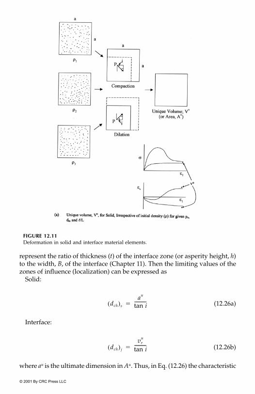
© 2001 By CRC Press LLC
represent the ratio of thickness (t) of the interface zone (or asperity height, h)to the width, B, of the interface (Chapter 11). Then the limiting values of thezones of influence (localization) can be expressed as
Solid:
(12.26a)
Interface:
(12.26b)
where au is the ultimate dimension in Au. Thus, in Eq. (12.26) the characteristic
FIGURE 12.11Deformation in solid and interface material elements.
dch( )s
au
tan i-----------�
dch( ) j
vru
tan i-----------�

© 2001 By CRC Press LLC
length is proportional to disturbance, Du, as Du for solids � Au�A, and forinterface, Du � , where � ultimate dilation when �n � 0, Fig. 11.6(b).
Furthermore, consider the following form of Eq. (12.22):
(12.27)
Assume that the incremental analysis is performed at the same level ofstrain increment, � � , Fig. 12.12(a) (Chapter 13). Then, Eq. (12.27)can be expressed as
(12.28)
FIGURE 12.11(continued)
vru�vr
0 vr0
d�˜
a 1 D�( )C˜
i d �˜
i DC˜
c d �˜
c� dD �
˜c
�˜
i�( ) �
d�˜
i d�˜
a d�˜
c
d�˜
a 1 D�( )C˜
i DC˜
c R˜
T�˜
c�˜
i�( ) [ ]d �
˜i C
˜DSC d �
˜i
�� �

© 2001 By CRC Press LLC
Here, D and (dD), Eq. (4.14), Chapter 4, are functions of Du, A, Z, � andd�, e.g.,
(12.29)
The constitutive matrix, in Eq. (12.28), includes the effects of both theplastic strains (� ) and gradient of plastic strains (d� ). Thus, the DSC model allowsfor the gradients of plastic strains in addition to the strains, and can be consid-ered to allow for nonlocal effects similar to those provided by the gradient-enriched models, Eq. (12.10) (10). Additional derivations to show the inclu-sion of gradient effects in the DSC are given in (29).
Now, consider the simple one-dimensional (uniaxial) form of Eq. (12.27),Fig. 12.12(b):
(12.30)
FIGURE 12.12Incremental iterative analysis at constant strain level.
R˜
R˜
T R˜
T Du, A, Z, �, d�( )�
C˜
DSC
d�a 1 D�( )Eid�
i D Ecd�c dD �
c�
i�( ) � �

© 2001 By CRC Press LLC
The computed value of d� a is limited with respect to the ultimate distur-bance, Du:
(12.31)
As Du � 1, � � 0, � � 0, dDu � 0 and � 0, the com-puted value of (d� a)u � 0. Hence, at localization corresponding to Du, thereare always nonzero values of and (� ). In other words, localizationoccurs at nonzero energy dissipation.
In view of the above, the DSC allows for nonlocal effects, microcrack inter-action and characteristic dimension. As a result, it avoids spurious meshdependence. Examples to illustrate these capabilities are given subsequently.
12.7.1 Approximate Decoupled DSC
The foregoing considerations apply when the coupled DSC, Eq. (12.28), leadsto the following (FE) equations:
(12.32)
where � dV is the stiffness matrix, is the incremental(RI) displacement vector and is the applied load vector. As noted before,
is nonsymmetric and becomes negative definite after the peak. Conver-gent computer results are obtained during incremental analysis at the samelevels of strains ( � � ). Then the observed stress is found for Eq.(12.28). Details are given in Chapter 13.
As discussed in Chapter 13, an approximate and decoupled but efficientprocedure can be developed and used. Here, the FE equations are first solvedonly for the RI response:
(12.33)
where � dV, is the RI elastoplastic constitutive matrix. Theincrement RI stress as is found as
(12.34)
and the FA stress is defined based on given assumptions, such as the criticalstate (Chapters 3 and 4):
(12.35)
Then the observed stress, , is found by using Eq. (12.28) through an iterativeprocedure in which the disturbance based on the stress-strain model from theobserved behavior is used as a convergence parameter (Chapter 13), Fig. 12.13.
d�a( )u 1 Du�( )Ei d�
i DuEcd�c dDu �
c�
i�( )u �
Ei Ec d�i d�
c�
c�
i�( )u
d�a d�
i d�a
K˜
DSC dqi
˜� dQ
˜�
K˜
DSC �VB˜
T C˜
DSC B˜
dq˜
i
dQ˜K
˜DSC
d�˜
a d�˜
i d�˜
c
K˜
i dq˜
i� dQ
˜
i�
K˜
i �vB˜
T C˜
ep B˜
C˜
ep
d�˜
i
d�˜
i C˜
ep d�˜
i��
d�˜
c C˜
c d�˜
i��
d�˜
a

© 2001 By CRC Press LLC
FIGURE 12.13Approximate decoupled analysis and critical disturbances.
© 2001 By CRC Press LLC
For the foregoing uncoupled procedure, insofar as the FE computer analysisis concerned, there arise no questions of nonlocality and spurious meshdependence, because the computer solution is based on the continuum plastichardening response, Fig. 12.13. However, the calculation of does involveaveraging and the effect of coupling between the RI and RI responses.
12.7.2 Instability Through Disturbance
The limiting case, Eq. (12.18), results because the states of stress,strain and disturbance (damage) that define the changing (nonlinear)response reach certain critical values. For instance, in the case of nonlinearelastic behavior, the tangent elastic modulus, Et, approaches zero at the peak,and leads to the limiting condition.
In the DSC, the disturbance, D, is involved in the definition of the tangentmatrix, , Eq. (12.28). Hence, the examination of the variation of distur-bance during deformation can provide the conditions in Eqs. (12.18) and(12.21). For instance, when the disturbance reaches the value of Dcm, microc-racking can initiate; when it reaches the value of Dp at the peak, localizationmay initiate; when it reaches the critical value, Dc, material instability (failure,liquefaction) can initiate; and when it reaches the value of Df, engineeringfailure or fracture occurs, Fig. 12.13 (b).
Assuming that the incremental iterative calculations are performed at thesame level of strains, i.e., � � , the matrix is given by
(12.36)
Figure 12.13(c) shows schematic variations of the first two terms, the lastterm and in Eq. (12.36) (29). When D � 0, � , i.e., the initialmatrix is the same as that for the RI (e.g., elastoplastic) material. The matrix
� at the peak, and then it becomes negative (definite) during the fall-ing (softening) region of the stress-strain response. During the softeningregion when → 0, initiation of instability or failure occurs.
If the FA material does not carry any stress as in the classical damage model(38), i.e., � , as D → 1, → o as dD → o. However, if the FA materialcan carry stress, i.e., � , will be positive with small magnitudedepending on the properties of the FA material. In that case, microcrackingleading to fracture and instability, which initiates when D � Dc, will growand the final failure will occur when D � Df, Fig. 12.13(a), due to large mag-nitudes of the FA zones.
Hence, the initiation of microcracking and of failure (instability) and frac-ture can be identified on the basis of threshold values of disturbance such asDcm and Dc, which are determined from appropriate laboratory tests.
The foregoing states of the matrix at the material level will be reflectedat the structural system level, in stiffness matrix, , Eq. (12.21):
(12.37a)
d�˜
a
C˜
0˜,�
C˜
DSC
d�˜
i d�˜
a d�˜
c C˜
DSC
C˜
DSC 1 D�( )C˜
i DC˜
c R˜
�˜
c�˜
i�( ) �
C˜
DSC C˜
DSC C˜
i
C˜
DSC 0˜
C˜
DSC
C˜
c 0˜
C˜
DSC
C˜
c o˜ C
˜DSC
C˜
DSC
K˜
DSC
K˜
DSCdq˜
i dQ˜
�

© 2001 By CRC Press LLC
where
(12.37b)
which will become negative definite after the peak, and at D � Dc, it will indi-cate structural instability, as → 0.
Now, we present a mathematical derivation of instability in the DSC.
12.7.3 Stability Analysis of DSC
Mathematical stability analyses of various constitutive models with theenrichments such as Cosserat and gradient theories are presented in a num-ber of publications (10–12). The stability analysis of the DSC for the one-dimensional specialization together with simple examples is presentedbelow. First, we present an analytical stability condition for the one-dimen-sional DSC model, Davis (66). Then stability analyses for the DSC using com-puter finite element method are presented.
12.7.4 Stability Condition for One-Dimensional DSC Model
Consider the one-dimensional problem, Fig. 12.14. The one-dimensional rate(incremental) constitutive, evolution, equilibrium and strain-displacementequations are given by
(12.38a)
(12.38b)
(12.38c)
(12.38d)
(12.38e)
(12.38f)
FIGURE 12.14One-dimensional idealization: stability analysis (66).
K˜
DSC B˜
T C˜
DSC B˜
Vdv
��
K˜
DSC
�a 1 D�( )�
i D�c D �
c�
i�( ) �
�i Ci
�i
��
�c Cc �
c��
D � ��
���x------- �u�
�u�x------ ��

© 2001 By CRC Press LLC
where the superscript a, i, and c denote observed, RI, and FA states, the over-dot denotes rate, � is a scalar parameter, � is the density, u is the displacement[Fig. (12.14)], � is the observed strain, and it is assumed that the strains in theRI and FA parts are equal.
Let Do, �o, and uo relate to a homogeneous steady state condition.Consider a perturbation from the steady state, Fig. 12.15, with the resultingquantities as
(12.39)
where k is the material parameter, is the frequency, t is time, and o denotesthe steady state condition. Now the rate of various quantities in Eq. (12.39)and their derivatives with respect to x can be defined; for example:
(12.40a)
(12.40b)
and so on.Now use of Eq. (12.39) in Eq. (12.38a) leads to
(12.41a)
FIGURE 12.15Perturbation from steady state: stability analysis.
�oa, �o
i , � oc,
�a
�oa
�a ei kx t( )
� �
�i
�oi
�i ei kx t( )� �
�c
�oc
�c ei kx t( )
� �
D Do D ei kx t( )� �
� �o � ei kx t( ) �
u uo uei kx t( ) �
�a
�aiei kx t( )
�
��a
�x-------- �
aikei kx t( )�
�ai 1 Do�( )�i Do�
c i �oc
�oi
�( )Di � �

© 2001 By CRC Press LLC
or
(12.41b)
Similarly, Eqs. (12.38b), (12.38c) and (12.38d) become
(12.42a)
(12.42b)
and
(12.42c)
(12.42d)
Now, the equilibrium and strain-displacement relations, Eqs. (12.38e) and(12.38f) become
(12.43a)
(12.43b)
Equations (12.41) to (12.43) with Eq. (12.38a) can be written in the matrixnotation as
(12.44)
By setting the determinant of the matrix in Eq. (12.44) to zero, we obtain
(12.45a)
or
(12.45b)
�a 1 D�( )�
i Do�c D �c
c�o
i�( ) �
�i Ci
��
�c Cc
���
D ��, if �ei kx t( ) o��
D �� �, if �ei kx t( ) o��
k�a
� u�
ku ��
1 Do 1� Do� �oi
�oc
� 0 0
0 1 0 0 Ci� 0
0 0 1 0 Cc� 0
0 0 0 1 �� 0k 0 0 0 0 ��
0 0 0 0 � k
�a
�i
�c
D
�
u
000000
�
��2 k2
� �oi
�oc
�( ) DoCc Ci Do 1�( ) �[ ]� 0�
2
k2------ Ci 1 Do�( ) CcDo � �o
i�o
c�( )�
�------------------------------------------------------------------------------------�

© 2001 By CRC Press LLC
If Eq. (12.42d) is used, we have
(12.46)
In Eq. (12.45), �k is the wave velocity, (1 � Do) and Do are the tangentmoduli or slopes at the steady state, Fig. 12.16, and denotes thereduction or increase in the effective tangent modulus corresponding to thefirst two terms, for positive or negative �, respectively. Assume that isalways positive, Fig. 12.16; a positive value of � denotes increase in the distur-bance for the softening response, while a negative value denotes decrease indisturbance for stiffening or healing, Fig. 12.16.
Now, to investigate stability, we examine the condition when the term onthe right-hand side, Eq. (12.45), becomes negative. Consider the possibilitywith respect to Eq. (12.42c):
(12.47)
FIGURE 12.16Stress-strain response: softening and stiffening.
2
k2------
Ci 1 Do�( ) Cc D� o ��( ) �oi
�oc
�( )�
�---------------------------------------------------------------------------------------------------�
Ci Cc
� �oi
�oc
�( )
�oi
�oc
�
Ci 1 Do�( ) CcDo � �oi
�cc
�( ) 0��

© 2001 By CRC Press LLC
Now, for the RI behavior (say, linear or nonlinear elastic or plastic harden-ing, Fig. 12.16), and as 0 � D � 1, we have
(12.48)
which represents the instability criterion. Now, with and � and Eq. (12.48) becomes
(12.49)
With Eq. (12.42d), we have for instability criterion
(12.50a)
(12.50b)
12.8 Examples
Now we consider examples to illustrate various characteristics of the DSC,namely, spurious mesh dependence, localization and instability.
Example 12.1 Spurious Mesh DependenceA number of computer analyses using the finite element procedures describedin Chapter 13 were performed to study the issue of spurious mesh depen-dence with the DSC. Results from two of the studies are described below.
The first study involved computer solutions based on the general DSCequations in which the constitutive matrix , Eq. (12.28), is nonsymmetricand becomes negative definite after the peak and during the softening region.
Figure 12.17(a) shows the finite element mesh for a concrete specimentested under multiaxial loading conditions (67). Four different meshes with4, 16, 64 and 256 elements (8-noded isoparametric) were used.
The specimen was subjected to prescribed compressive displacement load-ing with increment � 0.05 mm on the top surface. The test specimen involvedno confining stress; hence, the plane-strain idealization was used as anapproximation. In the incremental analysis, strains were averaged over theGauss points for the quarter of the specimen (29).
�oi
�oc 1
�--- Ci 1 Do�( ) CcDo [ ]��
� dD�d�� Cc
d� i
d�-------- Cc d� c
d�--------- ,�
�oi
�oc d�
dD-------- d�
i
d�-------- 1 Do�( ) d�
c
d�--------Do ��
Ci 1 Do�( ) Cc Do � �oi
�oc
�( ) 0� � �
�oi
�oc 1
�--- Ci 1 Do�( ) CcDo [ ]��
C˜
DSC
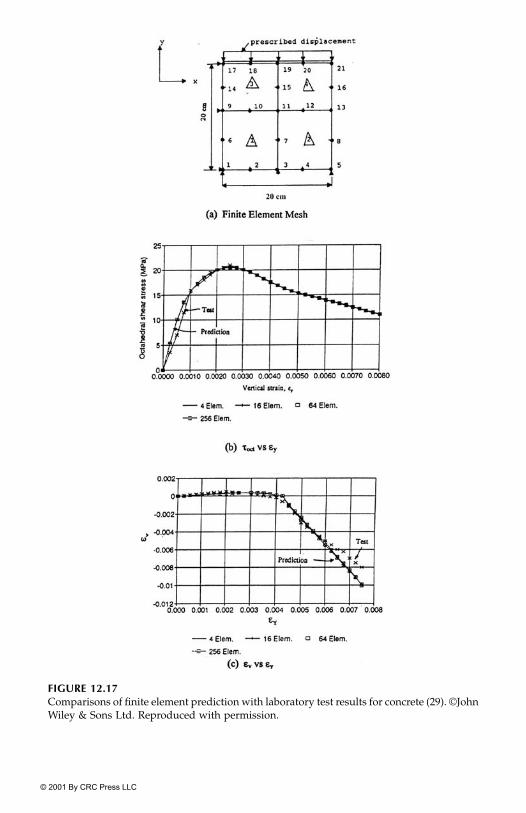
© 2001 By CRC Press LLC
FIGURE 12.17Comparisons of finite element prediction with laboratory test results for concrete (29). ©JohnWiley & Sons Ltd. Reproduced with permission.

© 2001 By CRC Press LLC
The material of the specimen was concrete and was characterized as elas-toplastic (�0-model) with disturbance (Chapters 4 and 7). The parametersused are given below (29, 62, 64):
E � 37.00 GPa, � � 0.25;
� � 0.0678, � � 0.755, n � 5.237
a1 � 4.61 � 10�11, � � 0.8262;
A � 688.00, Z � 1.502, Du � 0.875.
Figures 12.17(b) and (c) show comparisons between the computed octahedralstress, �oct, vs. axial strain, �y, and volumetric strain, �y, vs. �y and the observeddata from the laboratory tests. It can be seen that the results involve essentiallyno spurious mesh sensitivity, and that the predictions compare well with thelaboratory observations.
The second study involved the approximate uncoupled FE procedure inwhich the incremental analysis, Eq. (12.33), is performed only for the RIresponse with as the constitutive matrix, and observed response is thencomputed by using Eq. (12.28).
The finite element analysis for the second study was performed for tensionand compression loading on a rectangular zone made of Pb�Sn (40/60) solder.Three meshes with 16, 64, and 256 elements were used; Fig. 12.18 shows typ-ical mesh with 8-noded isoparametric elements (68).
The solder material was characterized using the DSC model in which theRI material was modelled as elastoplastic (HISS-�0) model (Chapter 7), andthe FA material was assumed to carry hydrostatic stress. The elastic, plasticand disturbance parameters used are given below:
E � 15.7 GPa, � � 0.40;
� � 0.00081, � � 0.00, n � 2.10
a1 � 0.78 � 10�5, � � 0.46, R � 208 MPa;
A � 0.102, Z � 0.676, Du � 0.90
The load was applied in increments. For the compression case, a total loadof 36.5 MPa was applied in 50, 100 and 100 steps with increments � 0.60, 0.05and .015 MPa, respectively. For the tension case, the total load of 33.5 MPa wasapplied in 50, 100 and 280 steps with increments � 0.40, 0.10 and 0.0125 MPa.
Figure 12.19 shows computed axial stress (�y) vs. axial stress (�y) at point A,Fig. 12.18, for both the observed (a) and RI (i) responses; similar plots werealso obtained at other points (B to F) marked in Fig. 12.18. It can be seen that
C˜
ep

© 2001 By CRC Press LLC
the results are independent of the mesh; i.e., there is no spurious mesh depen-dence. It may be noted that the stresses and strains are computed in the FE (DSC)analysis at specific points such as A, without averaging (over Gauss) points.
Example 12.2 LocalizationAs discussed earlier, strain localization occurs in a deforming material, par-ticularly during the softening zone, Fig. 12.2(a). Differences of opinion havebeen expressed regarding the existence and location of possible slip linesthrough the study of the acoustic tensor (10, 69). For example, Zienkiewiczand Huang (70) have stated that “…. Acoustic tensor is a very unreliable indi-cator and most of the reported difficulties result simply from using an incor-rect finite element approximation in the solution of plasticity problemsinvolved.” The DSC model allows for localization and can also be used foradaptive mesh refinement (see Chapter 13).
To illustrate the computational and localization capabilities of the DSC, anumber of problems have been solved; they include one-dimensional bar
FIGURE 12.18Finite element mesh with 256 elements: tensile (and compressive) loadings (68).
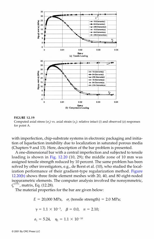
© 2001 By CRC Press LLC
with imperfection, chip-substrate systems in electronic packaging and initia-tion of liquefaction instability due to localization in saturated porous media(Chapters 9 and 13). Here, description of the bar problem is presented.
A one-dimensional bar with a central imperfection and subjected to tensileloading is shown in Fig. 12.20 (10, 29); the middle zone of 10 mm wasassigned tensile strength reduced by 10 percent. The same problem has beensolved by other investigators, e.g., de Borst et al. (10), who studied the local-ization performance of their gradient-type regularization method. Figure12.20(b) shows three finite element meshes with 20, 40, and 80 eight-nodedisoparametric elements. The computer analysis involved the nonsymmetric,
, matrix, Eq. (12.28).The material properties for the bar are given below:
E � 20,000 MPa, �t (tensile strength) � 2.0 MPa;
� � 1.1 � 10�3, � � 0.0, n � 2.10;
a1 � 5.24, �1 � 1.1 � 10�10
FIGURE 12.19Computed axial stress (�y) vs. axial strain (�y): relative intact (i) and observed (a) responsesfor point A.
C˜
DSC

© 2001 By CRC Press LLC
Disturbance
The elastic parameter (E) and �t were the same as those used by de Borst,et al. (10). The parameters for the plasticity (�0) model and disturbance wereevaluated based on the stress-strain curves given in (10). A small non-linear-ity with plasticity response was considered. The three curves correspondingto different values of the ratio of the characteristic length (�) to the length ofthe bar (L) were smoothed and extended to approach residual stresses ofabout 1.00, 0.80 and 0.50 MPa, respectively. The disturbance parameters werefound to be dependent of the ratio, ��L, as shown above.
Figure 12.21 shows computed results using the DSC in terms of strain (�) vs.length, and stress (�) vs. displacement (u) for three meshes with 20, 40 and 80,8-noded isoparametric elements, Fig. 12.20(b), and for ��L � 0.05. Figure 12.21(a)shows consistent convergence for strains with the meshes. With the gradientmodel, the strain approached the value of about 1.0 � 10�3 with 160 elements(10); the DSC model shows similar value with 80 elements.
The expression for the width of localization zone, w, is given by (10):
(12.51)
The localization width, w, predicted by the DSC model, Fig. 12.21(a), isabout 33 mm. This gives the value of � from Eq. (12.51) as 5.25 mm, whichcompares well with � � 5.00 mm used in (10). It may be mentioned that the
FIGURE 12.20Tension bar with imperfection. ©John Wiley & Sons Ltd. Reproduced with permission.
Case �/L A Z Du
1 0.10 500 2.37 0.502 0.05 530 1.35 0.603 0.025 550 0.31 0.75
w 2���

© 2001 By CRC Press LLC
DSC does not involve � as a (direct) parameter; hence, the comparison ismeant as an indirect validation. The computed results in terms of stress vsdisplacements, Fig. 12.21(b), also show trends similar to those presented byde Borst et al. (10).
Computed DSC results for ��L � 0.10, 0.05, and 0.025 for strain vs. lengthand stress vs. displacement for the 80-element mesh, Fig. 12.20(b), are shownin Fig. 12.22. The localization width, w, increases with �/L, Fig. 12.22(a), indi-cating more brittle response for smaller values of �. The values of � using Eq.(12.51) for the three ratios are found to be 3.2, 5.25 and 7.00 mm, while thoseused in (10) were 2.50, 5.00 and 10.00 mm, respectively. The overall magni-tudes of stress and trends in Fig. 12.22(b) are similar to those from the gradi-ent theory (10). However, there are some differences due to reasons such as:(1) the �0-plasticity model with disturbance is used in the DSC, while de Borstet al. (10) used an elastoplastic (Drucker-Prager) model with the gradientenrichments, (2) the smoothing and digitization of stress-strain curves, and (3)in the DSC, the plastic strains are developed from the beginning, while in theDrucker-Prager model, they develop only after the (peak) stress is reached.
FIGURE 12.21Computed results using DSC for ��L � 0.05 (29). ©John Wiley & Sons Ltd. Reproduced withpermission.
FIGURE 12.22Computed results for 80-element mesh for three ��L ratios: (1) 0.10, (2) 0.05, (3) 0.025 (29).©John Wiley & Sons Ltd. Reproduced with permission.
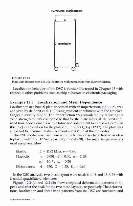
© 2001 By CRC Press LLC
Localization behavior of the DSC is further illustrated in Chapter 13 withrespect to other problems such as chip-substrate in electronic packaging.
Example 12.3 Localization and Mesh DependenceLocalization in a biaxial plate specimen with an imperfection, Fig. 12.23, wasanalyzed by de Borst et al. (10) using gradient enrichment with the Drucker-Prager plasticity model. The imperfection was simulated by reducing itsyield strength by 10% compared to that for the plate material. de Borst et al.used four-node elements with a bilinear displacement field and a Hermitian(bicubic) interpolation for the plastic multiplier (�), Eq. (12.12). The plate wassubjected to incremental displacement � 0.0001 m at the top nodes.
The DSC model was used here with the RI response characterized as elas-toplastic with the HISS-�0 plasticity model (30). The material parametersused are given below:
Elastic: E � 1192 MPa, � � 0.49;Plasticity: � � 0.001, � � 0.00, n � 2.10;
a1 � 10�10, �1 � 0.20Disturbance: A � 530, Z � 1.35, Du � 0.60
In the DSC analysis, two mesh layout were used: 6 � 18 and 13 � 36 with8-noded quadrilateral elements.
Figures 12.24(a) and 12.24(b) show computed deformation patterns at thepeak and after the peak for the two mesh layouts, respectively. The deforma-tions, localization and shear band patterns from the DSC are consistent and
FIGURE 12.23Plate with imperfection (10, 30). Reprinted with permission from Elsevier Science.

© 2001 By CRC Press LLC
show essentially the same trends as in the analysis by de Borst, et al. (10);some differences between the two results can be due to factors such as thedifferent material model and element orders used in the present analysis.Figure 12.25 shows load displacement curves from the two mesh layouts;they indicate no significant mesh dependence. In Fig. 12.25, F is the loadinduced at the top, B is the width of the plate, is the observed or actualstress, �top is the displacement at the top and H is the height of the plate.
FIGURE 12.24Deformation patterns in imperfect bar for 13 � 36 mesh (30). Reprinted with permissionfrom Elsevier Science.
FIGURE 12.25Load-displacement curves for 6 � 18 and 13 � 36 meshes (30). Reprinted with permissionfrom Elsevier Science.
�

© 2001 By CRC Press LLC
These results show that the DSC model provides consistent and satisfac-tory localization and shear banding and avoids the spurious mesh depen-dence without the need for external enrichments.
Example 12.4 Instability in the DSCThe first example involves analysis of instability using Eq. (12.49) for givennumerical stress-strain data. Consider the observed stress-strain response,Fig. 12.26(a). The RI response is simulated as nonlinear using hyperbolicfunction as
(12.52a)
where a � 1�Ei and b � 1��u are parameters, Ei is the initial modulus, �u is theultimate asymptotic stress, �i is the RI stress and � is the strain. The values ofa and b for the RI curve, Fig. 12.26(a), are obtained as 2.33 � 10�5 and 0.0133,respectively (Chapter 5). The FA response is simulated as linear elastic givenby
(12.52b)
where � c is the stress in the FA material.The instability criterion, Eq. (12.49), is expressed as
(12.53)
where � is computed as
(12.54)
FIGURSE 12.26Stress-strain behavior and variation of tangent modulus.
�i �
a b� ----------------�
�c 850 ���
�oi
�oc 1
�--- d�
i
d�-------- 1 Do�( ) d�
c
d�--------Do ��
�dDd�--------
Dom 1 Do
m�
�om 1
�om
�-----------------------------��

© 2001 By CRC Press LLC
where m is the incremental step. Disturbance, D, is expressed as a function ofstrain, �, and can be computed by using the stress-strain response as
(12.55)
where is the measured stress at a (steady) state. Table 12.1 shows the cal-culations of various quantities.
For the strain (�) levels, before about 0.003, stability is indicated as per Eq.(12.53). At and after � � 0.003, the values of the left-hand side in Eq. (12.53)become greater than those of the right-hand side (RHS), indicating instability.The instability occurs at strain levels beyond the peak stress, � a, of about 35N/mm2, in the softening zone at disturbance D � 0.45. Figure 12.26(b) showsa plot of the RI tangent modulus (d� i�d�) vs. strain.
Liquefaction Instability The second example involves instability thatindicates liquefaction in saturated (soil) media. Conventionally, liquefaction isconsidered to initiate when the excess pore fluid (water) pressure that increasesduring (cyclic) loading equals the initial effective pressure (Chapter 9). In theDSC, the instability leading to initiation of liquefaction occurs when the micro-structure reaches the critical threshold state at the critical disturbance, Dc
(Chapters 9 and 13).Figure 12.27 shows the dimensions of a (cubical) test specimen idealized as
axisymmetric. The specimen is first subjected to initial effective confiningstress, , and then deviatoric (shear) stress, �1 � where �1 is the axial stress.
The specimens of saturated Ottawa sand at relative density (Dr � 60%)were tested under three different initial confining stresses, � 69, 138 and207 kPa (71–73). The laboratory test behavior in terms of applied deviatoricstress vs. time, strain vs. time and excess pore water pressure vs. time, as wellas plots of effective stress, , � – p, where is the total stress, and p is the
TABLE 12.1
Instability Calculations
� � a � i � c D dD/d� �i � � c R.H.S.�
0.00021 8.05 8.05 0.18 5.40 � 10�8 0.0043 7.87 80 � 105
.00054 17.71 17.71 0.46 4.2 � 10�6 115.55 17.25 215.50
.00092 25.00 25.90 0.78 0.100 280.27 25.12 60.100.00129 29.00 31.88 1.10 0.144 146.69 30.78 77.730.00175 33.00 37.57 1.49 0.222 93.61 36.08 103.820.0020 35.00 41.00 1.70 0.250 151.40 39.30 50.00
.0030 34.00 47.47 2.55 0.440 148.29 44.92 21.24
.0040 33.00 52.29 3.40 0.546 90.03 48.89 20.98
.0060 29.00 58.20 5.10 0.709 65.07 53.10 10.030.0080 24.00 61.68 6.80 0.843 72.37 54.88 3.110.010 18.00 63.98 8.50 0.978 33.00 55.48 0.7540.020 18.00 69.13 17.00 0.981 24.63 52.13 2.22
�R.H.S. � 1dD�d�( )
---------------------- d�i
d�-------- 1 D�( ) d�
c
d�--------D
D�o
i�o
a�
�oi
�oc
�-------------------�
�oa
�o �o,
�o
� � �t
�t

© 2001 By CRC Press LLC
FIGURE 12.27Finite element mesh and loading for triaxial test specimen (72). ©John Wiley & Sons Ltd.Reproduced with permission.
FIGURE 12.28Disturbance and curvature vs. deviatoric plastic strain trajectory as function of cycles, N:
� 69 kPa. ©John Wiley & Sons Ltd. Reproduced with permission.�o

© 2001 By CRC Press LLC
pore water pressure are given in Chapter 9. Disturbance, D, is expressed as
(12.56)
where i, a and c denote RI, observed and FA states, respectively.The (average) material parameters for the sand are given by
E � 193.00 MPa, � � 0.38;� � 1.713, � � 0.0, n � 2.45;a1 � 0.845, �1 � 0.0215;
� 0.20, � � 0.019, e o � 0.593;A � 4.22, Z � 0.43, Du � 0.99.
Figures 12.28 to 12.30 show plots of disturbance vs deviatoric plastic straintrajectory, �D (or number of cycles, N) and the curvature (D!) vs. �D(N) for thethree confining pressures (72). Here,
FIGURE 12.29Disturbance and curvature vs. deviatoric plastic strain trajectory as function of cycles, N:
� 138 kPa. ©John Wiley & Sons Ltd. Reproduced with permission.�o
D�
i�
a�
�i
�c
�------------------�
m

© 2001 By CRC Press LLC
(12.57)
The critical disturbance, Dc, occurs when D! is the minimum; it can also befound approximately at the intersection of tangents to the earlier and later(saturation) parts of the disturbance curve. The values of Dc for the three con-fining pressures are found to be 0.82, 0.830 and 0.850, respectively, with cor-responding cycles 5, 7 and 8. These cycles compare well with those observedin the tests (Chapter 9) when the pore pressure becomes approximately equalto the initial confining pressure. Thus, the critical disturbance, Dc, identifiesthe initiation of instability leading to liquefaction.
Finite element analyses with one-element mesh, Fig. 12.27, were performedin which the initial confining pressures were first applied, followed by incre-mental increase of �1 � . Figure 12.31 shows variations of the trace of theconstitutive matrix, with �D (as the function of N), for � 69, 138 and207 kPa. The trace, which represents the sum of eigen values, first decreasesand then assumes a minimum value. Thereafter, it stabilizes to a small valueas per Eq. (12.28) in the ultimate region when D approaches Du � 0.99, and
FIGURE 12.30Disturbance and curvature vs. deviatoric plastic strain trajectory as function of cycles, N:
� 207 kPa. ©John Wiley & Sons Ltd. Reproduced with permission.�o
D!d2Dd�D
2---------- AZ�D
z�2 exp ADz
�( ) Z 1� AZ�Dz
�( )� �
�o
CiiDSC �

© 2001 By CRC Press LLC
dD � 0. The trace assumes minimum values at �D � 0.20, 0.15 and 0.10,respectively, for the three confining pressures. These values correspondclosely with the values at the initiation of liquefaction corresponding to Dc �0.82, 0.830 and 0.850 in Figs. 12.28 to 12.30 at cycles to liquefaction, Nc � 5, 7,and 8, respectively. Similar results were obtained with respect to plots of thetrace of the stiffness matrix, vs. �D. Thus, the mathematical propertiesof the constitutive and stiffnesses matrices in the DSC correlate well with lique-faction instability identified through critical values of disturbance and theexperimental response of the sand.
FIGURE 12.31Variation of for different . ©John Wiley & Sons Ltd. Reproduced with permission.Cii
CDC�o
KiiDSC
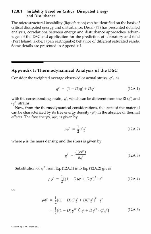
© 2001 By CRC Press LLC
12.8.1 Instability Based on Critical Dissipated Energyand Disturbance
The microstructural instability (liquefaction) can be identified on the basis ofcritical dissipated energy and disturbance. Desai (73) has presented detailedanalysis, correlations between energy and disturbance approaches, advan-tages of the DSC and application for the prediction of laboratory and field(Port Island, Kobe, Japan earthquake) behavior of different saturated sands.Some details are presented in Appendix I.
Appendix I: Thermodynamical Analysis of the DSC
Consider the weighted average observed or actual stress, , as
(12A.1)
with the corresponding strain, , which can be different from the RI ( ) and strains.
Now, from the thermodynamical considerations, the state of the materialcan be characterized by its free energy density (� a) in the absence of thermaleffects. The free energy, �� a, is given by
(12A.2)
where � is the mass density, and the stress is given by
(12A.3)
Substitution of from Eq. (12A.1) into Eq. (12A.2) gives
(12A.4)
or
(12A.5)
�˜
a
�˜
a 1 D�( )�˜
i D�˜
c �
�˜
a�˜
i
�˜
c( )
��a 1
2---�
˜a�˜
a�
�˜
a� e�
a( )��
˜a
----------------�
�˜
a
��a 1
2--- 1 D�( )�
˜i D�
˜c
[ ]T�˜
a��
��a 1
2--- 1 D�( )C
˜i�˜
i DC˜
c�˜
c [ ]T
�˜
a��
12--- 1 D�( )�
˜aT C
˜i�˜
i D�˜
aT C˜
c�˜
c� [ ]�
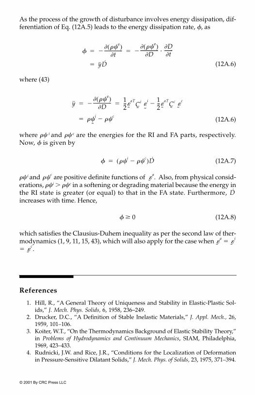
© 2001 By CRC Press LLC
As the process of the growth of disturbance involves energy dissipation, dif-ferentiation of Eq. (12A.5) leads to the energy dissipation rate, ", as
(12A.6)
where (43)
(12A.6)
where �� i and �� c are the energies for the RI and FA parts, respectively.Now, " is given by
(12A.7)
�� i and are positive definite functions of . Also, from physical consid-erations, ��i � ��c in a softening or degrading material because the energy inthe RI state is greater (or equal) to that in the FA state. Furthermore, increases with time. Hence,
(12A.8)
which satisfies the Clausius-Duhem inequality as per the second law of ther-modynamics (1, 9, 11, 15, 43), which will also apply for the case when �� .
References
1. Hill, R., “A General Theory of Uniqueness and Stability in Elastic-Plastic Sol-ids,” J. Mech. Phys. Solids, 6, 1958, 236–249.
2. Drucker, D.C., “A Definition of Stable Inelastic Materials,” J. Appl. Mech., 26,1959, 101–106.
3. Koiter, W.T., “On the Thermodynamics Background of Elastic Stability Theory,”in Problems of Hydrodynamics and Continuum Mechanics, SIAM, Philadelphia,1969, 423–433.
4. Rudnicki, J.W. and Rice, J.R., “Conditions for the Localization of Deformationin Pressure-Sensitive Dilatant Solids,” J. Mech. Phys. of Solids, 23, 1975, 371–394.
"� ��
a( )�t
-----------------�� ��
a( )�D
-----------------��D�t--------�� �
yD�
y� ��
a( )�D
-----------------�12---�
˜aT
C˜
i �˜
i 12---�
˜aT
C˜
c �˜
c�� �
��˜
i��
c��
" ��i
��c
�( )D�
��c
�˜
a
D
" 0�
�˜
a�˜
i
�˜
c

© 2001 By CRC Press LLC
5. Mailer, G. and Hueckel, T., “Nonassociated and Coupled Flow Rules of Elas-toplasticity for Rock-like Materials,” Int. J. Rock Mech. Min. Sc., 16, 1979, 77–92.
6. Walgraet, D. and Aifantis, E.C., “On Theories in Formulation and Stability ofDislocation 429. Patterns, I-III,” Int. J. Eng. Science, 12, 1985, 1351–1372.
7. Kratochvil, J., “Dislocation Pattern Formulation in Metals,” Revue Phys. Appl.,23, 1988, 419–429.
8. Benallal, A., Billarden, R. and Geymonat, G., “Localization Phenomena at theBoundaries and Interfaces of Solids,” Proc., Third Int. Conf. on Constitutive Lawsfor Engineering Materials: Theory and Application, Desai, C.S. et al. (Editors), Univ.of Arizona, Tucson, AZ, 1991, 387–390.
9. Valanais, K.C., “A Global Damage Theory and Hyperbolicity of the WaveProblems,” J. of Appl. Mech., ASME, 58, 1991, 311–316.
10. de Borst, R., Sluys, L.T., Mühlhaus, H.B. and Pamin, J., “Fundamental Issuesin Finite Element Analyses of Localization of Deformation,” Int. J. Eng. Com-putations, 10, 1993, 99–121.
11. Bazant, Z.P. and Cedolin, L., Stability of Structures, Oxford Univ. Press, NewYork, 1991.
12. Mühlhaus, H.B. (Editor), Continuum Models for Materials with Microstructure,John Wiley, Chichester, U.K., 1995.
13. Bazant, Z.P., “Nonlocal Damage Theory Based on Micromechanics of CrackInteractions,” J. Eng. Mech., ASCE, 120, 3, 1996, 593–617.
14. Desai, C.S., “Constitutive Modelling Using the Disturbed State as Microstruc-ture Self-Adjustment Concept,” Chapter 8, in Continuum Models for Materialswith Microstructure, H.B. Mühlhaus (Editor), John Wiley, Chichester, U.K., 1995.
15. Desai, C.S. and Toth, J., “Disturbed State Constitutive Modelling Based onStress-Strain and Nondestructive Behavior,” Int. J. Solids Struct., 33, 11, 1996,1619–1650.
16. Schreyer, H.L. and Cheng, Z., “One-Dimensional Softening with Localization,”J. Appl. Mech., s53, 1986, 791–799.
17. Lasry, D. and Belytchko, T., “Localization Limiters in Transient Problems,” Int.J. Solids Struct., 24, 1988, 581–597.
18. Needleman, A., “Material Rate Dependence and Mesh Sensitivity in Localiza-tion Problems,” Int. J. Comp. Meth. Appl. Mech. Eng., 67, 1988, 69–86.
19. Simo, J.C., “Strain Softening and Dissipation: A Unification of Approaches,” inCracking and Damage, Strain Localization and Size Effect, Mazars, J. and Bazant,Z.P. (Editors), Elsevier, London, 1989, 440–461.
20. Desai, C.S., Kundu, T. and Wang, G., “Size Effect on Damage Parameters forSoftening in Simulated Rock,” Int. J. Num. Analyt. Meth. Geomechanics, 14, 1990,509–517.
21. Loret, B. and Prevost, J.H., “Dynamic Strain Localization in Fluid-SaturatedMedia,” J. of Eng. Mech., ASCE, 117, 1991, 907–922.
22. Zienkiewicz, O.C. and Huang, M., “Localization Problems in Plasticity UsingFinite Elements and Adaptive Remeshing,” Int. J. Numer. Analy. Meth. Geomech.,19, 1995, 127–148.
23. Sulen, J., Vardoulakis, I., and Papamichos, E., “Microstructure and Scale Effectin Granular Rocks,” Chapter 7 in in Continuum Models for Materials with Micro-structure, Mühlhaus, H.B. (Editor), John Wiley, U.K., 1995, 201–237.
24. van Mier, J.G.M., “Mode-I Fracture of Concrete: Discontinuous Crack Growthand Crack Interface Grain Bridging,” J. of Cement Concrete Res., 21, 1991, 1–15.
25. van Mier, J.G.M., Fracture Processes of Concrete, CRC Press, Boca Raton, FL, 1997.

© 2001 By CRC Press LLC
26. Gutierrez, M.A. and de Borst, R., “Studies in Material Parameter Sensitivity ofSoftening Solids,” Comp. Meth. in Appl. Mech. and Eng., 162, 1998, 337–350.
27. Bazant, Z.P. and Pijaudier-Cabot, G., “Measurement of Characteristic Lengthof Nonlocal Continuum,” J. of Eng. Mech., ASCE, 115, 4, 1989, 775–767.
28. Mühlhaus, H.B. and Vardoulakis, I., “The Thickness of Shear Bands in GranularMaterials,” Geotechnique, 37, 1987, 271–283.
29. Desai, C.S., Basaran, C. and Zhang, W., “Numerical Algorithms and MeshDependence in the Disturbed State Concept,” Int. J. Num. Meth. Eng., 40, 1997,3059–3083.
30. Desai, C.S. and Zhang, W., “Computational Aspects of Disturbed State Consti-tutive Models,” Int. J. Comp. Meth. Appl. Mech. Eng., 151, 1998, 361–376.
31. Oden, J.T. and Pires, E.B., “Nonlocal and Nonlinear Friction Laws and Varia-tional Principles for Contact Problems in Elasticity,” J. of Applied Mechanics, 50,1983, 67–75.
32. Pastor, M., Zienkiewicz, O.C., Vilotte, J.P. and Quecedo, M., “Mesh DependenceProblems in Viscoplastic Materials Under Quasi-static Loading,” in Computa-tional Plasticity: Fundamentals and Applications, Owen, D.R.J., et al. (Editors),Pineridge Press, Swansea, U.K., 1995.
33. Desai, C.S. and Abel, J.F., Introduction to the Finite Element Method, Van NostrandReinhold, New York, 1972.
34. Desai, C.S. and Kundu, T., Introductory Finite Element Method, CRC Press, BocaRaton, FL, 1999, under publication.
35. Sluys, L.J., “Wave Propagation, Localization and Dispersion in SofteningSolids,” Doctoral Dissertation, Delft University of Technology, The Nether-lands, 1992.
36. Wang, W.W., “Stationary and Propagative Instabilities in Metals—A Compu-tational Point of View,” Doctoral Dissertation, Delft Univ. of Technology, TheNetherlands, 1997.
37. Eringen, A.C., “A Unified Theory of Thermomechanical Materials,” Int. J. Eng.Sci., 4, 1966, 179–202.
38. Kachanov, L.M., Introduction to Continuum Damage Mechanics, Martinus NijhoftPublishers, The Netherlands, 1986.
39. Pijaudier-Cabot, G. and Bazant, Z.P., “Nonlocal Damage Theory,” J. Eng. Mech.,ASCE, 113, 1987, 1512–1533.
40. Krajcinovic, D., “Damage Mechanics,” Mech. Materials, 8, 1987, 117–197.41. Bazant, Z.P. and Lin, F.B., “Non-local Yield Limit Degradation,” Int. J. Num.
Meth. Eng., 26, 1988, 1805–1823.42. Bazant, Z.P. and Pijaudier-Cabot, G., “Nonlocal Continuum Damage, Localiza-
tion Instability and Convergence,” J. Appl. Mech., 55, 1988, 287–293.43. Lamaitre, J. and Chaboche, J.L., Mechanics of Solid Materials, Cambridge Univ.
Press, U.K., 1989, Dunod-Bordas, Paris, 1985.44. Mühlhaus, H.B., de Borst, R., Sluys, L.J. and Pamin, J., “A Thermodynamic
Theory for Inhomogeneous Damage Evolution,” Proc., 9th Int. Conf. on ComputerMethods and Advances in Geomechanics, Balkema, 1994, 635–640.
45. Pijaudier-Cabot, G., “Non Local Damage,” Chapter 4 in Continuum Models forMaterials with Microstructure, H.B. Mühlhaus (Editor), John Wiley, U.K., 1995,105–143.
46. Voyiadjis, G.Z. and Kattan, I., Advances in Damage Mechanics: Metals and MetalMatrix Composites, Elsevier Science Ltd., Oxford, U.K., 1999.

© 2001 By CRC Press LLC
47. Coleman, B.D. and Hodgden, M.L., “On Shear Bands in Ductile Materials,”Arch. Rational Mech. Analysis, 90, 1985, 219–247.
48. Aifantis, E.C., “The Physics of Plastic Deformation,” Int. J. of Plasticity, 3, 1987,211–247.
49. Zbib, H.M. and Aifantis, E.C., “On the Localization and Postlocalization Be-havior of Plastic Deformation, I, II, III,” Res. Mechanica, 23, 1988, 261–277,279–292, 293–305.
50. Mühlhaus, H.B. and Aifantis, E.C., “The Influence of Microstructure InducedGradients on the Localization of Deformation in Viscoplastic Materials,” ActaMechanica, 89, 1991, 217–231.
51. Vardoulakis, I. and Aifantis, E.C., “A Gradient Flow Theory of Plasticity forGranular Materials,” Acta Mechanica, 87, 1991, 197–217.
52. de Borst, R. and Mühlhaus, H.B., “Gradient-Dependent Plasticity: Formulationand Algorithmic Aspects,” Int. J. Num. Meth. Eng., 35, 1992, 521–539.
53. Oka, F., “A Gradient Dependent Elastic Model for Granular Materials andStrain Localization,” Chapter 5 in Continuum Models for Materials with Micro-structure, Mühlhaus, H.B. (Editor), John Wiley, U.K., 1995, 145–158.
54. Peerlings, R.H.J., de Borst, R., Brekelmans, W.A.M. and de Vree, J.H.P., “Gra-dient Enhanced Damage for Quasi-Brittle Materials,” Int. J. Numer. Meth. Eng.,39, 1996, 3391–3403.
55. Cosserat, E. and Cosserat, F., Theorie des Corps Deformables, Herman et Fils,Paris, France, 1909.
56. Eringen, A.C., “Theory of Micropolar Continuum,” Proc., 9th Midwestern Mech.Auf., Univ. of Wisconsin, Madison, WI, 1965, 23-40.
57. Eringen, A.C., “Theory of Micropolar Elasticity,” in Fracture, An Advanced Trea-tise, H. Liebowitz (Editor), Academic Press, New York, 1968.
58. Mühlhaus, H.B., “Application of Cosserat Theory in Numerical Solutions ofLimit Load Problems,” Ing.-Archiv, 59, 1989, 124–137.
59. Willam, K., Dietsobe, A., Iordache, M.M. and Steinmann, P., “Localization inMicropolar Continua,” Chapter 9 in Continuum Models for Materials with Micro-structure, Mühlhaus, H.B. (Editor), John Wiley, U.K., 1995.
60. Kröner, E., “Elasticity Theory of Materials with Long Range Cohesive Forces,”Int. J. Solids Struct., 3, 1967, 731–742.
61. Kubin, L.P. and Lepinoux, J., “The Dynamic Organization of Dislocation Struc-tures,” Proc., 8th Int. Conf. on Strength of Materials and Alloys, Tampere, 1988,35–39.
62. Frantziskonis, G. and Desai, C.S., “Constitutive Model with Strain Softening,”Int. J. Solids Struct., 23, 1987, 751–767.
63. Desai, C.S. and Hashmi, Q., “Analysis, Evaluation and Implementation of aNonassociative Model for Geologic Materials,” Int. J. of Plasticity, 5, 1989,397–420.
64. Desai, C.S. and Woo, L., “Damage Model and Implementation in NonlinearDynamic Problems,” Int. J. Comput. Mech., 11, 1993, 189–206.
65. Desai, C.S., Basaran, C., Dishongh, T. and Prince, J., “Thermomechanical Anal-ysis in Electronic Packaging with Unified Constitutive Model for Materials andJoints,” Components, Packaging and Manuf. Tech., Part B: Advanced Packaging,IEEE Trans., 21, 1, 1998, 87–97.
66. Davis, R.O., Private communication, 1998.67. Van Mier, J.G.M., “Strain Softening of Concrete under Multiaxial Loading Con-
ditions,” Ph.D. Dissertation, Eindhoran Univ. of Tech., The Netherlands, 1984.

© 2001 By CRC Press LLC
68. Whitenack, R., Private communication, 1999.69. Larsson, R., Runesson, K., and Ottoson, N.S., “Discontinuous Displacement
Approximation for Capturing Plastic Localization,” Int. J. Numer. Methods inEngng., 36, 1993, 2087–2105.
70. Zienkiewicz, O.C. and Huang, M., “Localization Problems in Plasticity UsingFinite Elements with Adaptive Remeshing,” Int. J. Numer. Analy. Meth. Geo-mech., 19, 1995, 127–148.
71. Gyi, M.M., “Multiaxial Cyclic Testing of Saturated Ottawa Sands,” M.S. Thesis,Dept. of Civil Eng. and Eng. Mechs., University of Arizona, Tucson, AZ, 1997.
72. Desai, C.S., Park, I.J., and Shao, C., “Fundamental Yet Simplified Model forLiquefaction Instability,” Int. J. Numer. Analyt. Meth. Geomechanics, 22, 1998,721–748.
73. Desai, C.S., “Evaluation of Liquefaction Using Disturbance and EnergyApproaches,” J. of Geotech. and Geoenv. Eng., ASCE, 126, 7, 2000, 618–631.

13Implementation of DSC in Computer Procedures
CONTENTS13.1 Finite Element Formulation
13.1.1 Incremental Equations13.2 Solution Schemes
13.2.1 FA Stress13.2.2 Observed Behavior
13.3 Algorithms for Creep Behavior13.3.1 Algorithms for Elastic, Plastic, Viscoplastic Behavior
with Thermal Effects13.3.2 Elastic Behavior13.3.3 Plane Stress13.3.4 Plane Strain13.3.5 Axisymmetric13.3.6 Thermoplastic Behavior13.3.7 Thermoviscoplastic Behavior13.3.8 DSC Formation
13.4 Algorithms for Coupled Dynamic Behavior13.4.1 Fully Saturated Systems13.4.2 Dynamic Equations13.4.3 Finite Element Formulation13.4.4 Time Integration for Dynamic Problems
13.5 Implementation13.6 Partially Saturated Systems13.7 Cyclic and Repetitive Loading
13.7.1 Unloading13.7.2 Reloading13.7.3 Cyclic-Repetitive Hardening
13.8 Initial Conditions13.8.1 Initial Stress13.8.2 Initial Disturbance
13.9 Hierarchical Capabilities and Options13.10 Mesh Adaption Using DSC
13.10.1 Prepeak Response
© 2001 By CRC Press LLC

13.10.2 Postpeak Response13.11 Examples of Applications
13.11.1 Laboratory Tests13.11.2 Field Validation13.11.3 Computer Results
13.12 Computer Codes
The incremental constitutive equations in the DSC and its hierarchical versionsare presented in Chapters 4–12. In this Chapter, we consider the implementationof the models in computer (finite element) procedures. The finite element static,dynamic and creep formulations are presented, together with details of a num-ber of schemes for the introduction of the DSC models in the computer proce-dures. Here, elastic, plastic, and creep models with disturbance are includedtogether with thermal effects. Use of the disturbance as the criterion for meshadaption is also described. A number of example problems are then presented.They include computational aspects such as the effect of (load) increments and awide range of problems from civil and mechanical engineering, electronic pack-aging, dynamics and earthquake engineering, solid mechanics and pavements.
13.1 Finite Element Formulation
The following formulations and algorithms are presented in the context ofthe finite element (FE) methods. However, they can be adopted, with somemodifications, for other numerical procedures such as the boundary elementmethod and finite difference technique.
With the displacement based FE method, the stationary potential energy orthe virtual work principle is often invoked to derive the element and assem-blage questions for problems discretized into FE meshes [Fig. 13.1 (1–4)].According to the virtual work principle, we can write
(13.1)
where and are the vectors of observed or actual stresses and strainscomponents, respectively, � denotes virtual quantity, V is the volume, is thevector of displacement components, is the vector of applied body forces,and is the vector of applied surface tractions on a part of the surface, S1. Thedisplacement vector = [u v w] at a point P (Fig. 13.1) is expressed as
(13.2)
where is the matrix of interpolation functions (of various orders) and is the vector of (observed) nodal displacements. The strain vector, isobtained from Eq. (13.2) as
(13.3)
��˜
a( )T�˜
a VdV
� �u˜
T X˜
V �u˜
T T˜
SdS1��d
V��
�˜
a �˜
a
u˜X
Tu˜
a( )T
u˜
a N˜
q˜
a�
N˜
q˜
a
�˜
a,
�˜
a N˜
�q˜
B˜
q˜
a� �
© 2001 By CRC Press LLC

where the prime denotes derivative and is the strain-displacementtransformation matrix. In general, is a 6 � 1 vector; however, for a two-dimensional (plane stress, plane strain, or axisymmetric) idealization, willhave three to four components (1–4).
Substitution of Eqs. (13.2) and (13.3) in Eq. (13.1) gives
(13.4)
As the virtual displacement, , is arbitrary, the FE equilibrium equationsresult as
(13.5a)
where is the applied load vector:
(13.5b)
FIGURE 13.1Schematic of finite element discretization.
B˜�
˜a
�˜
a
�q˜
a( )TB˜
T
V� �
˜a dV �q
˜
a( )T N˜
T X˜
V N˜
T T˜
SdV
��dV
��
�q˜
a
B˜
T�˜
a Vd� Q˜
�
Q˜
Q˜
N˜
TX˜
V N˜
TT˜
SdS1��d��
© 2001 By CRC Press LLC
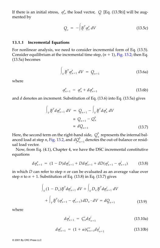
If there is an initial stress, , the load vector, [Eq. (13.5b)] will be aug-mented by
(13.5c)
13.1.1 Incremental Equations
For nonlinear analysis, we need to consider incremental form of Eq. (13.5).Consider equilibrium at the incremental time step, (n � 1), Fig. 13.2; then Eq.(13.5a) becomes
(13.6a)
where
(13.6b)
and d denotes an increment. Substitution of Eq. (13.6) into Eq. (13.5a) gives
(13.7)
Here, the second term on the right-hand side, represents the internal bal-anced load at step n, Fig. 13.2, and denotes the out-of-balance or resid-ual load vector.
Now, from Eq. (4.1), Chapter 4, we have the DSC incremental constitutiveequations
(13.8)
in which D can refer to step n or can be evaluated as an average value overstep n to n � 1. Substitution of Eq. (13.8) in Eq. (13.7) gives
(13.9)
where
(13.10a)
(13.10b)
�˜ o
a Q˜
Q˜
o B˜
T�˜ o
a Vd���
B˜
T�˜ n�1
a VdV
� Q˜
n�1�
�˜ n�1
a�˜ n
a d�˜ n�1
a��
B˜
Td�˜ n�1
a VdV
� Q˜
n�1 B˜
Td�˜ n
a VdV
���
Q˜
n�1 Qnb
�=
dQ˜
n�1=
Q˜
nb
dQ˜
n�1b
d�˜ n�1
a 1 D�( )d�˜ n�1
i Dd�˜ n�1
c dD �˜ n�1
c�˜ n�1
i�( )� ��
1 Dn�( )B˜
T�˜ n�1
id V Dn B˜
T�˜ n�1
cd VdV
��dV
�
B˜
T�˜ n�1
c�˜ n�1
i�( ) Dn dVd
V� dQ
˜n�1��
d�˜ n�1
i C˜ n
i d�˜ n�1
i�
d�˜ n�1
c 1 �( )C˜ n�1
c d�˜ n�1
i�
© 2001 By CRC Press LLC

Here, we used Eq. (4.5), i.e., � (1 � ) , where is the relative strain(motion) parameter. Now, substitution of Eqs. (13.10) in Eq. (13.9) leads to
(13.11)
Here is the vector of relative stresses in the FA and RIparts, and dDn � from Eq. (4.14). Now, writing
(13.12)
and substitution of from Eq. (13.3), we have
(13.13a)
FIGURE 13.2Incremental analysis.
d�˜ n�1
c d�˜ n�1
i
B˜
T1 Dn�( )C
˜ ni Dn 1 �( )C
˜ nc R
˜T�˜ n
r�� d�
˜ n�1i� dQ
˜n�1�
�˜ n�1
r�˜ n�1
c�˜ n�1
i��
R˜
Td�˜ n
n
C˜ n
DSC 1 Dn�( )C˜ n
i Dn 1 �( )C˜ n
c R˜
T�˜ n
r� ��
d�˜ n�1
i B˜
d q˜
n�1
i�
B˜
TC˜ n
DSCB˜
V dq˜
n�1
id
V� dQ
˜n�1�
© 2001 By CRC Press LLC
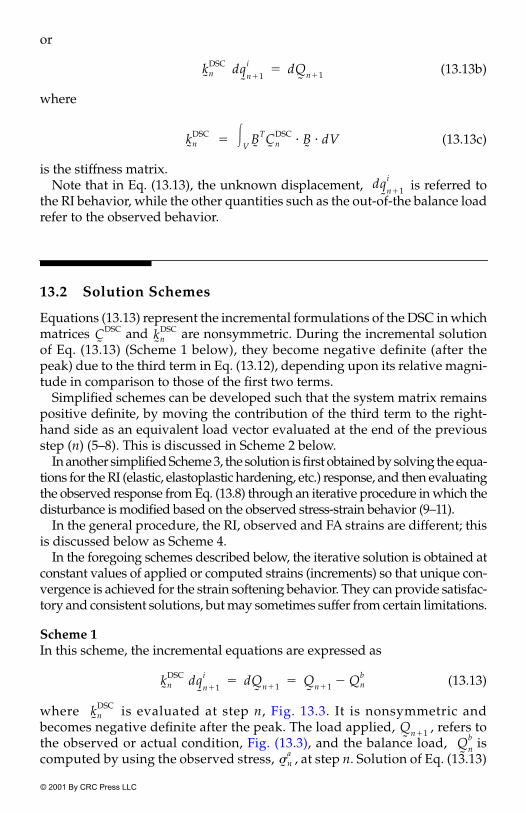
or
(13.13b)
where
(13.13c)
is the stiffness matrix.Note that in Eq. (13.13), the unknown displacement, is referred to
the RI behavior, while the other quantities such as the out-of-the balance loadrefer to the observed behavior.
13.2 Solution Schemes
Equations (13.13) represent the incremental formulations of the DSC in whichmatrices and are nonsymmetric. During the incremental solutionof Eq. (13.13) (Scheme 1 below), they become negative definite (after thepeak) due to the third term in Eq. (13.12), depending upon its relative magni-tude in comparison to those of the first two terms.
Simplified schemes can be developed such that the system matrix remainspositive definite, by moving the contribution of the third term to the right-hand side as an equivalent load vector evaluated at the end of the previousstep (n) (5–8). This is discussed in Scheme 2 below.
In another simplified Scheme 3, the solution is first obtained by solving the equa-tions for the RI (elastic, elastoplastic hardening, etc.) response, and then evaluatingthe observed response from Eq. (13.8) through an iterative procedure in which thedisturbance is modified based on the observed stress-strain behavior (9–11).
In the general procedure, the RI, observed and FA strains are different; thisis discussed below as Scheme 4.
In the foregoing schemes described below, the iterative solution is obtained atconstant values of applied or computed strains (increments) so that unique con-vergence is achieved for the strain softening behavior. They can provide satisfac-tory and consistent solutions, but may sometimes suffer from certain limitations.
Scheme 1In this scheme, the incremental equations are expressed as
(13.13)
where is evaluated at step n, Fig. 13.3. It is nonsymmetric andbecomes negative definite after the peak. The load applied, , refers tothe observed or actual condition, Fig. (13.3), and the balance load, iscomputed by using the observed stress, , at step n. Solution of Eq. (13.13)
k˜n
DSC dq˜
n�1
i dQ˜
n�1�
k˜n
DSC B˜
TC˜ n
DSC B˜
dV V
��
dq˜
n�1
i
C˜
DSC k˜n
DSC
k˜n
DSC dq˜
n�1
i dQ˜
n�1 Q˜
n�1 Qnb
�� �
k˜n
DSC
Q˜
n�1Q˜
nb
�˜ n
a
© 2001 By CRC Press LLC

provides the increments of RI displacement, , which are used to evalu-ate the RI strains, , and stress, , using the following equations:
(13.14)
and
(13.15)
where is the RI constitutive matrix which can be characterized by usingelastic, elastoplastic, etc. idealizations.
In the case of the elastoplastic (�0-model), the increment of RI stress, is corrected by using the drift correction procedure described in Chapter 7.Then the converged values, and the corresponding total stress, ,are calculated. The iterative procedure is performed at constant strain (incre-ment), � � , Fig. (13.3). Such constant value can be due to appliedstrains (displacement) or, in general, due to the computed strains as a result
FIGURE 13.3Incremental analysis at constant strain and disturbance.
dq˜
n�1
i
d�˜ n�1
i d�˜ n�1
i �( )
d�˜ n�1
i B˜
dq˜
n�1
i�
d�˜ n�1
i �( )C˜
id�˜ n�1
i�
C˜
i
d�˜ n�1
i �( )
d�˜ n�1
i�˜ n�1
i
d�˜
i d�˜
a d�˜
c
© 2001 By CRC Press LLC

of the applied load or stress. Such a procedure can lead to a uniqueconverged value of stress for a given strain and avoid the duality of strains ifconvergence is sought based on the applied stress.
Now, we need the FA stress and disturbance, Dn, for the calculation ofthe observed stress, , Eq. (13.8). Details of their calculations are given below.
13.2.1 FA Stress
The FA stress increment is expressed as
(13.16)
where � [1 1 1 0 0 0]. As discussed in Chapters 3 and 4, a number of sim-ulations are possible to characterize the FA state; e.g., (a) “void”, (b) hydrostaticstrength, and (c) critical state. These are discussed below.
Void: If the FA part is treated like a “void”, as in the classical damagemodel (12), it can carry no stress at all. Then
(13.17)
This assumption is considered to be unrealistic because the micro-cracked or FA part, which is surrounded by the RI parts, can possesscertain strength.Hydrostatic strength: If the FA state is assumed to carry hydrostatic stressor mean pressure, it acts like a constrained liquid. Then it can carry noshear stress, but can carry hydrostatic stress, Eq. (4.27). Therefore,
(13.18a)
(13.18b)
The FA response can be characterized based on the bulk modulus,, for the FA material. As a simple approximation, it can be assumed
that the hydrostatic stresses in the RI and FA parts are equal, i.e.,
(13.18c)
Then Eq. (4.19) can be used. Alternatively, Eq. (13.19b) below can beused to define the FA response.Critical state: As discussed in Chapter 4, the constitutive equations thatgovern the response of the FA material at the critical state are given by
(13.19a)
Q˜
n�1( )
d�˜
c( )d�
˜ n�1a
d�˜ n�1
c dS˜ n
c 13---dJ1n
c I˜
��
I˜
T
�nc d�
˜ n�1c 0
˜� �
dS˜ n�1
c0˜
�
13---dJ
˜n�1c 0
˜�
K˜
c
dJ˜
1 n�1( )c dJ
˜1 n�1( )i
�
J2Dc mJ1
c�
© 2001 By CRC Press LLC

and
(13.19b)
or
(13.19c)
Then the matrix, , is defined by assuming that , and theshear stress, , is defined based on Eq. (4.31). The constitutiveequations with the assumption of critical state are derived in Chapter4, Eqs. (4.35), in which the incremental critical stress is given by
(13.20a)
(13.20b)
where
Here, the RI stresses are computed at step (n � 1) and is computedusing Eq. (13.19c) and as
(13.21)
where eo is the initial void ratio and e � �(1 � eo)�ii .Disturbance: The disturbance, D, at steps n and n � 1 is computed as
(13.22a)
ec eoc
� ln J1c 3pa ( )��
J1c 3paexp
eoc ec
�
�----------------
�
C˜
c J1i J1
c�
J2Dc
d�n�1c
�J1
i
�---- 1 eo�( )
mS˜
i
J2Di
----------- 13---I
˜�
I˜d�n�1
c
J1cm
J2Di
----------- C˜
i 13---I
˜C
i S˜
iTS˜
i
2J2i
------------ C˜
i�� d�
˜ n�1i
�
� M˜
d�˜ n�1
c N˜
d�n�1i
�
M˜
J1 n�1( )c
�---------------� 1 eo�( ) mS
˜i
J2D n�1( )i
----------------------13--- I
˜�
N˜
J1 n�1( )c
m
J2D n�1( )i
---------------------- C˜
i 13--- I
˜C˜
i�
S˜
iTS˜
i
2 J2Di
--------------- C˜
i�
�
Jc1
dJ1c
dJ1 n�1( )c J1 n�1( )
c
�--------------- 1 e0�( )�ii n�1( )
c�
Dn Du 1 e�A�Dn
z
� �
© 2001 By CRC Press LLC

and
(13.22b)
where, as an approximation, �D can be evaluated based on the RIresponse as
(13.22c)
Disturbance based on the observed response can be used in an itera-tive procedure; this is described later, in the context of the simplifiedprocedure (Scheme 3).The increment, dDn can be found approximately as
(13.23a)
or by using Eq. (4.14b) as
(13.23b)
The computations are performed at constant strain, � � ,and the foregoing procedure yields and , which in turn,can be used to evaluate total values as
(13.24a)
(13.24b)
(13.24c)
(13.24d)
The balanced load, is found as
(13.26)
With the above quantities at (n � 1), we revise the constitutive matrixat n � 1 as
(13.27)
Here, as � � , � 0 in Eq. (13.12) are assumed.Now, we apply the next load increment, , solve Eq. (13.13) andrepeat the foregoing procedure.
Dn�1 Du 1 e�A�D n�1( )
z
� �
�Di dE
˜pi( )T
dE˜
pi�1 2
�
dDn Dn�1 Dn��
dDn R˜ n�1
T d�˜
i�
d�˜
i d�˜
a d�˜
c
d�˜ n�1
a d�˜ n�1
a
�˜ n�1
a �˜ n
a d�˜ n�1
a��
�˜ n�1
a�˜ n
a d�˜ n�1
a��
�˜ n�1
c �˜ n
c d�˜ n�1
c��
�˜ n�1
c�˜ n
c�˜ n�1
c��
Q˜
n�1b
Q˜
n�1b B
˜T�n�1
a Vd��
C˜ n�1
DSC 1 Dn�1�( )Cn�1i DnCn�1
c R˜
T�n�1
r� ��
d�˜
i d�˜
a d�˜
c
Q˜
n�2
© 2001 By CRC Press LLC

Iterations. The drift correct procedure (Chapter 7) can entail iterationsduring the incremental analysis during which the stress convergesfrom to , Fig. 13.3. Iterations can be performed in the com-putation of , Eq. (13.8), during which the disturbance is revised;this is described later (Scheme 3).
Scheme 2The term, or dD in Eq. (13.11) is moved to the right-hand sideas
(13.28a)
or
(13.28b)
where
The matrices and are positive definite, and is evaluated at theend of the previous step n, based on the known values of the terms involved.The solution of Eq. (13.28) gives the incremental RI displacements, strainsand stresses, and the procedure for the evaluation of the observed stress,
, is similar to that in Scheme 1.It may be noted that the modification of equations in this scheme that yields
positive definite stiffness matrix does not change the nature of the basic prob-lem. Also, depending upon the relative magnitude of in comparison to
, convergence and stability problems may arise for some situations (6).
Scheme 3This scheme is conceptually similar to Scheme 2 in which the stiffness matrix ispositive definite (5–7). The incremental nonlinear analysis is first performed toevaluate the RI response in which the stiffness matrix is positive definitebecause it relates to the continuum characterization such as nonlinear elasticand elastoplastic (9,11). The FA response is defined based on the assumptionsdescribed under Scheme 1. Then the observed stress is computed by using Eq.(13.8) and an iterative procedure during which the disturbance is revised.
Figure (13.4) shows a schematic of the procedure. The RI response is firstevaluated by applying a load increment, , relevant to the RI response, in
�˜ n�1
i �( )�˜ n�1
i
d�˜ n�1
a
R˜
T�˜ n
r�˜
c�˜
i�( )
B˜
T1 Dn�( )C
˜ ni Dn 1 �( )C
˜ nc
� B˜
q˜
n�
idV
� dQ˜
n�1 R˜ n
T�˜ n
r B˜
VdV
���
knDSC
dqn�1i dQ
˜n�1 Q
˜nr
��
knDSC
B˜
TC˜
DSCB˜
VV
��
Q˜
nr R
˜T�˜ n
r B˜
Vd��
C˜
DSCk˜
nDSC
Q˜
nr
d�˜ n�1
a
Q˜
nr
d�˜ n�1
a
dQ˜
i
© 2001 By CRC Press LLC

which the RI stress, , is evaluated using the drift correction procedure. Theobserved stress, , is evaluated at constant value of the computed RI strain,
� � � . Details of Scheme 3: The incremental FE equations for the RI response (elas-tic, elastoplastic hardening, etc.) are given by
(13.29a)
where is the incremental vector of RI displacements:
(13.29b)
and
(13.29c)
The matrices and are positive definite, as the RI response is charac-terized as nonlinear elastic or elastoplastic hardening (�0-model), etc.
FIGURE 13.4 RI-based incremental procedure for scheme 3.
�˜
i
�˜
a
d�˜
i d�˜
a d�˜
c d�˜
k˜n
i dqn�1i dQn�1
i Qn�1i Qn
b i( )�� �
dq˜
n�1
i
k˜n
i B˜
TC˜ n
i B˜
Vd��
Q˜
nb i( ) B
˜T�˜ n
b i( ) Vd��
C˜ n
i k˜n
i
© 2001 By CRC Press LLC

Solution of Eq. (13.29) yields and then incremental strains andstresses as
(13.30a)
(13.30b)
The drift correction procedure leads to , Fig. 13.3(a). The total quanti-ties are evaluated as
(13.31a)
and
(13.31b)
13.2.2 Observed Behavior
The observed incremental stress, , Eq. (13.8) is now found, with appro-priate model for the FA behavior, as
(13.32)
where the superscript (1) denotes the first iteration. As and arebased on the deviatoric plastic strains for the observed response, their valuesare not available for the current step (n � 1). Hence, they are computed byassuming that for the first iteration:
(13.33)
and hence,
(13.34a)
and
(13.34b)
dq˜
n�1
i
d�˜ n�1
i B˜
dq˜
n�1
i�
d�˜ n�1
i �( )C˜ n
i d�˜ n�1
i�
d�˜ n�1
i
�˜ n�1
i �˜ n
i d�˜ n�1
i��
�˜ n�1
i�˜ n
i d�˜ n�1
i��
d�˜ n�1
a
d�˜ n�1
a 1( ) 1 Dn�11( )
�( )d�˜ n�1
i Dn�11( ) d�
˜ n�1c dDn�1
1( )�˜ n�1
c�˜ n�1
i�( )� ��
Dn�11( ) dDn�1
1( )
�D n�1( )a 1( )
�D n�1( )i 1( )
�
Dn�11( ) Du 1 e
�A�Dz
�( )�
dDn�11( ) R
˜ n�11( )T d�
˜ n�1i
�
© 2001 By CRC Press LLC

where . The term, can also be computed by using Eq.(13.23a), which for the first iteration will be zero. Now, the total observedstress, , (Fig. 13.5) is found as
(13.35)
which would usually not be the “correct” value as the disturbance is foundon the basis of the RI strains.
In order to improve the computed values in Eqs. (13.32) and (13.35), an iter-ative procedure can be used, in which the modified value of the observedplastic strain increment is found approximately as (Fig. 13.5)
(13.36)
where
and is the elastic constitutive matrix computed by assuming that the unload-ing elastic moduli in the RI and FA states are equal. Alternatively, modified
FIGURE 13.5Iterative method for scheme 3.
�D �D n�1( )a 1( )
� dDn�11( )
�˜ n�1
a 1( )
�˜ n�1
a 1( ) 1 Dn�11( )
�( )�˜ n�1
i Dn�11( )
�n�1c
��
d�˜ n�1
ap 1( ) C˜
e( )�1d�n�1
a 1( )�
d�n�1a 1( )
�˜ n�1
i�n�1
a 1( )��
C˜
e
© 2001 By CRC Press LLC

value of the observed elastic moduli can be adopted by using the followingequation (13)
(13.37)
where is the initial elastic modulus and Ec is the modulus in the FA region,Fig. 13.5. The Poisson’s ratio in can be assumed to be constant.
The modified (increased) observed plastic strains, , for the second iter-ation are now given by
(13.38)
Then, the revised deviatoric plastic strain trajectory for the second iterationis evaluated as
(13.39)
in which the second term on the right-hand side is computed by usingEq. (13.22c); the deviatoric plastic strains, , relate to the observed strains,Eq. (13.36). The disturbance is revised by using Eq. (13.22), and the observedstresses are computed for the second and the subsequent iterations ( j) as
(13.40)
The iterations are continued until convergence at j � m, which can be defined as
(13.41)
At the end of iterations, m, various observed quantities are found for the loadincrement, , as
(13.42a)
(13.42b)
(13.42c)
and the total stresses using Eq. (13.35). The observed or actual load incre-ments, , can be found as
(13.43)
En�1a 1 Dn�1
1( )�( )Eo Dn�1
1( ) Ec��
Eo
C˜
e
�˜ n�1
ap 2( )
�˜ n�1
ap 2( ) �˜ n�1
ap 1( )� d�
˜ n�1ap 1( )
�
�D n�1( )a 2( )
�D n�1( )a 1( ) d�D n�1( )
a 2( )��
dE˜
p
�n�1a j( ) 1 Dn�1
j( )�( )�
˜ n�1i Dn�1
j�˜ n�1
c��
d�Da j�1( )
d�Da j( )------------------ � 10�6�( )�
Q˜
n�1i
d�n�1a m( ) 1 Dn�1
m( )�( )d�
˜ n�1i Dn�1
m( ) d�˜ n�1
c dDn�1m( )
�˜ n�1
c�˜ n�1
i�( )� ��
d�˜ n�1
a m( ) d�˜ n�1
i m( )�
�˜ n�1
a m( ) �˜ n�1
i�
dQn�1a
dQ˜
n�1a( ) B
˜T
�˜ n�1
a m( )d Vd��
© 2001 By CRC Press LLC

Then, we proceed to the next load increment, n � 2, and so on.The foregoing procedure involves the basic solution for the RI response, in
which the system matrix is positive definite. However, the coupling betweenthe RI and FA responses, which affects the observed response, is incorporatedthrough the iterative procedure in which the disturbance refers to theobserved behavior, defined on the basis of the laboratory test data.Scheme 4
In the foregoing three schemes, the FE equations, Eq. (13.13), involve solu-tions for the RI displacements, strains, etc. As described in Chapter 4, it ispossible to formulate the equations in terms of the observed strains and dis-placements by postulating relations between the FA and RI, and RI andobserved strains, Eqs. (4.49); a schematic is shown in Fig. 13.6. The procedureis described in Chapter 4, and would lead to different strains in the RI,observed and FA states. Further investigation would be required for thisscheme, particularly with respect to convergence and computational effort.Hence, at this time, we recommend use of Schemes 1 to 3, and in particularScheme 3, which is found to provide convergent and satisfactory results withconsiderable computational efficiency for many problems solved, includingthose presented later.
13.3 Algorithms for Creep Behavior
Description of the models based on the multicomponent DSC and overlayapproach for viscoelastic, viscoplastic and elastoviscoplastic behavior is pre-sented in Chapter 8. Now, we present algorithms for implementing typicalcreep models in computer (FE) procedures.
FIGURE 13.6Schematic of RI, FA and observed strains in material element.
© 2001 By CRC Press LLC

13.3.1 Algorithms for Elastic, Plastic, Viscoplastic Behaviorwith Thermal Effects
Among the factors to be considered for thermal response are (1) the existenceof “initial” strains due to the (known) temperature, and (2) temperaturedependence of material parameters during thermomechanical (cyclic) load-ing. First, we present algorithmic aspects for initial strains.
13.3.2 Elastic Behavior
In the case of elastic behavior, for isotropic material, the effect of known tem-perature change causing initial strains are expressed as follows:
(13.44)
where � [�x �y �z 0 0 0], � [T T T 0 0 0], and dT is the temper-ature change = T � T0, where T0 is the initial (previous) temperature, T is theco-efficient of thermal expansion, and T is the current temperature. For two-dimensional idealizations, Eq. (13.44) is specialized as follows:
13.3.3 Plane Stress
(13.45)
13.3.4 Plane Strain
(13.46)
where E and ν are the elastic parameters.
13.3.5 Axisymmetric
(13.47)
�˜ o
˜ T dT�
�˜ o
T˜ T
�x T( ) T dT�
�y T( ) T dT�
�xy T( ) 0.0�
�x T( ) T dT 1 ��( )�
�y T( ) T dT 1 ��( )�
�xy T( ) 0.0�
�z T( ) ET dT��
�r T( ) T dT�
�z T( ) T dT�
�� T( ) T dT�
�rz T( ) 0.0�
© 2001 By CRC Press LLC

Then the incremental elastic constitutive relation is given by
(13.48)
where is the elastic (tangent) constitutive matrix, and , , and d�(T)are the vectors of total, elastic and thermal strains, respectively.
If the parameters E and v vary with temperature, they can be expressed interms of temperature as (10, 14):
(13.49a)
(13.49b)
where Er and vr are values at reference temperature, Tr (e.g., room tempera-ture 23�C or 300 K), and cT and cν are parameters found from laboratory tests.
13.3.6 Thermoplastic Behavior
The normality rule gives the increment of plastic strain vector (T) as(11,14,15)
(13.50)
where Q is the plastic potential function; for associative rule, Q ≡ F, where F isthe yield function (Chapters 6 and 7). Now, the total incremental strain vector
is given by
(13.51a)
where (T) is the strain vector due to the temperature change. Hence,
(13.51b)
and
(13.51c)
d�˜
C˜
e d�˜
e�
C˜
ed�
˜d�
˜T( )��
C˜
e d�˜
d�˜
e
E ErTTt-----
CT
�
� �rTTr-----
C�
�
d�˜
d�˜
p T( ) ��Q �, �, T( )
��˜
------------------------------�
d�˜
t
d�˜
t T( ) d�˜
e T( ) d�˜
p T( ) d�˜
T( )� ��
d�˜
d�˜
e T( ) d�˜
��Q��
˜
-------- d�˜
T( )���
d�˜
C˜
e T( )d�˜
e�
C˜
e T( ) d�˜
e�
�Q��
˜
--------� TI˜1
0 dT� �
© 2001 By CRC Press LLC

where � [1 1 0] for the two-dimensional case, and [1 1 1 0 0 0] for thethree-dimensional case.
Now, the consistency condition gives
(13.52a)
Therefore,
(13.52b)
Then, use of Eqs. (13.51) and (13.52) gives
(13.53a)
Therefore,
(13.53b)
The parameters in the elastoplastic model, e.g., HISS-�0, can be expressedas a function of temperature as
(13.54)
where P is any parameter such as E, ν, Eq. (13.49); �, �, R, n, Eq. (7.1); a1, �1,Eq. (7.11); Pr is its value at reference temperature Tr , and c is parameter foundfrom laboratory tests.
13.3.7 Thermoviscoplastic Behavior
The total temperature dependent strain rate vector, , is assumed to be thesum of the thermoelastic strain rate, , thermoviscoplastic strain rate,
, and the thermal strain rate due to temperature change dT, , as
(13.55)
I˜1
0
dF �˜
, �, T( ) 0�
dF �FT
��˜
--------- d�˜
�F��------ d�
�F�T------- dT�� 0� �
�
�FT
��˜
--------- C˜
e T( )d�˜
�F�T------- dT T
�FT
��˜
---------C˜
e T( )I˜
odT��
�FT
��˜
--------- C˜
e T( )�Q��
˜
-------- �F��------
�QT
��˜
----------- �Q��
˜
--------
1 2
�
-----------------------------------------------------------------------------------------------------------�
d�˜
C˜
e T( ) I˜
�QT
��˜
----------- �F��
˜
-------C˜
e T( )
�FT
��˜
--------- C˜
e T( )�Q��
˜
-------- �F��------ �QT
��˜
----------- �Q��
˜
--------
1 2
�
-----------------------------------------------------------------------------�
d�˜
�
C˜
e T( ) TI˜
oT
�Q��
˜
-------- �FT
��˜
---------C˜
e T( )I˜
o �F�T------- �Q
��˜
--------�
�FT
��˜
--------- C˜
e T( )�Q��
˜
-------- �F��------ �QT
��˜
----------- �Q��
˜
--------
1 2
�
----------------------------------------------------------------------------�
dT�
P T( ) PrTTr-----
c
�
�˜�
˜e T( )
�˜
vp T( ) �˜
T( )
�˜
�˜
e T( ) �˜
vp T( ) �˜
T( )� ��
© 2001 By CRC Press LLC

Here, the thermoviscoplastic strain is contributed by creep and temperatureeffects.
With Perzyna’s (16) viscoplastic theory, Eq. (8.2d) (Chapter 8), Eq. (13.55)can be written as
(13.56)
where � and � are temperature dependent fluidity parameter and flow func-tion, respectively. Then the constitutive equations are given by
(13.57)
Viscous or creep behavior requires integration in time. The thermovisco-plastic strain rate (Chapter 8) is evaluated at time step n, Fig. 13.7. Then thestrain rate at step (n � 1) can be expressed by using Taylor series expansionas (14, 17)
(13.58)
where is the stress increment, is the temperature increment, and , denote gradient matrices at time step, n; their details are given in Eq. (8.45),
Chapter 8.
FIGURE 13.7 Time integration for viscoplastic strains.
�˜
�˜
e T( ) � T( )��F T( )
Fo------------
��F��
˜
------- �˜
e T( )���
�˜˙ C
˜e T( ) �
˜� � T( )��
F T( )Fo
------------ ��F
��˜
------- � �˜
T( ) �
�˜
vp T( )n+1�˜
vp T( )n
� �˜
vp T( )n
��˜
------------------------� ��˜ n
��˜
vpT( )n
�T------------------------ dTnI
˜��
�˜
vp T( )n G˜ 1n d�
˜ n G˜ 2n dTn I
˜� ��
��˜
n dTn G˜ 1
n
G˜ 2
n
© 2001 By CRC Press LLC
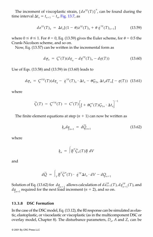
The increment of viscoplastic strain, , can be found during thetime interval �tn � tn�1 � tn, Fig. 13.7, as
(13.59)
where 0 � � � 1. For � � 0, Eq. (13.59) gives the Euler scheme, for � � 0.5 theCrank-Nicolson scheme, and so on.
Now, Eq. (13.57) can be written in the incremental form as
(13.60)
Use of Eqs. (13.58) and (13.59) in (13.60) leads to
(13.61)
where
The finite element equations at step (n � 1) can now be written as
(13.62)
where
and
Solution of Eq. (13.62) for allows calculation of , , and required for the next load increment (n � 2), and so on.
13.3.8 DSC Formation
In the case of the DSC model, Eq. (13.12), the RI response can be simulated as elas-tic, elastoplastic, or viscoelastic or viscoplastic (as in the multicomponent DSC oroverlay model, Chapter 8). The disturbance parameters, Du, A and Z, can be
d�vp T( ){ }n
d�vp T( )n �tn 1 ��( )�
vp T( )n � �˜
vp T( )n�1�[ ]�
d�˜ n C
˜e T( ) d�
˜ nd�
˜vp T( )n� d�
˜T( )�( )�
d�˜ n C
˜evp T( ) d�
˜ n�˜
vp T( )n �tn �G˜ 2n �tndTnI
˜�˜
T( )���( )�
C˜
T( ) C˜
evp T( ) Ce T( ) I˜
�C˜
e T( )G˜ 1n �tn�
�1� �
k˜ndq
˜n+1
dQ˜
n+1�
k˜n B
˜TC
˜n T( )B
˜Vd��
dQ B˜
TC˜
nT( ) �
˜vp
�tn dV dQ˜
n�1�V
��
dq˜
n�1d�n+1
vp T( ) d�˜ n�1
vp T( )dq
˜n+1
© 2001 By CRC Press LLC
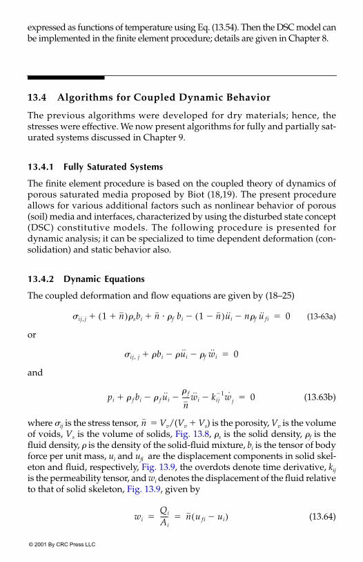
expressed as functions of temperature using Eq. (13.54). Then the DSC model canbe implemented in the finite element procedure; details are given in Chapter 8.
13.4 Algorithms for Coupled Dynamic Behavior
The previous algorithms were developed for dry materials; hence, thestresses were effective. We now present algorithms for fully and partially sat-urated systems discussed in Chapter 9.
13.4.1 Fully Saturated Systems
The finite element procedure is based on the coupled theory of dynamics ofporous saturated media proposed by Biot (18,19). The present procedureallows for various additional factors such as nonlinear behavior of porous(soil) media and interfaces, characterized by using the disturbed state concept(DSC) constitutive models. The following procedure is presented fordynamic analysis; it can be specialized to time dependent deformation (con-solidation) and static behavior also.
13.4.2 Dynamic Equations
The coupled deformation and flow equations are given by (18–25)
(13-63a)
or
and
(13.63b)
where �ij is the stress tensor, � Vv/(Vv � Vs) is the porosity, Vv is the volumeof voids, Vs is the volume of solids, Fig. 13.8, �s is the solid density, �f is thefluid density, � is the density of the solid-fluid mixture, bi is the tensor of bodyforce per unit mass, ui and ufi are the displacement components in solid skel-eton and fluid, respectively, Fig. 13.9, the overdots denote time derivative, kij
is the permeability tensor, and wi denotes the displacement of the fluid relativeto that of solid skeleton, Fig. 13.9, given by
(13.64)
�ij , j 1 n�( )�sbi n �f bi 1 n�( ) ui� n�f u fi�� � 0�
�ij , j �bi � ui� �f wi�� 0�
pi � f bi � f ui�� f
n----- wi� kij
�1wj˙�� 0�
n
wiQi
Ai----- n u fi ui�( )� �
© 2001 By CRC Press LLC

where Qi is the volume of fluid moving through an area of the skeleton normalto the ith direction, and Ai is the area normal to the ith direction (i � 1, 2, 3).
Equations (13.63) represent coupled differential equations with two vari-ables u and w. Formulation based on these equations is general, and isreferred to as u – w. If the relative acceleration, , between the solid and fluiddisplacement is ignored, Eqs. (13.63) lead to the u – p formulation, in which pis the (excess) fluid (pore water) pressure (22). For quasistatic problems, suchas consolidation, .
13.4.3 Finite Element Formulation
The approximation functions for u and w are expressed as (Fig. 13.10) (24)
(13.65a)
and
(13.65b)
FIGURE 13.8Porous saturated material element and porosity (24).
w
u w 0� �
ui Nua Ui
a�
wi Nwb Wi
b�
© 2001 By CRC Press LLC

FIGURE 13.9Deformations in two phase element.
FIGURE 13.10Finite element discretization and approximation function (24).
© 2001 By CRC Press LLC

where ui and wi (i � 1, 2, 3) are the solid displacements and relative displace-ments at a point, respectively; Nu and Nw are the interpolation functions corre-sponding to u and w, respectively; a � 1, 2, …Nue, b � 1, 2, … Nwe; Nue, Nwe �node numbers per element for u and w, respectively; and Ui and Wi denotethe nodal solid and relative displacements, respectively.
Use of the virtual work principle and substitution of various quantities andderivatives, Eq. (13.65), lead to the following finite element equations (24):
(13.66)
where a, c � (1 to NN); b, d � (1 to MM) with NN = MM = number of nodesin the whole domain, and i, j � (1, 2, 3), and
(13.67a)
(13.67b)
(13.67c)
(13.67d)
(13.67e)
(13.67f)
(13.67g)
In Eqs. (13.66) and (13.67), the integration domain V is the whole volumeand S the whole boundary, as sums of element volumes and surfaces. Equa-tion (13.66) has c, d, and j as dummy indices (summation indices), and a, b,and i as free indices. Therefore, there are (NN � MM) � 3 equations in Eq.(13.66). �ij and p in the third term on the left side in Eq. (13.66) are expressedin the incremental form as
(13.68a)
Muuijac Muwij
ad
Mwuijbc Mwwij
bd
U jc
W jd
0 0
0 Cwwijbd
U jc
W jd
Nu ,i
a�ij Vd
V�
Nw ,ib p Vd
V�
� �f ui
a
f wib
�
Muuijac
�ij �Nua Nu
a VdV
��
Muwijad
�ij � f Nua Nw
d VdV
��
Mwuijbc
�ij � f Nwb Nu
c VdV
��
Mwwijbd
�ij
� f
n-----Nw
b Nwd Vd
V��
Cwwijbd kij
�1Nwb Nw
d VdV
��
f uia Nu
a Ti S �biNua Vd
V��d
S��
f wib pNw
b ni S �f biNwb Vd
V��d
S��
d�ij Cijk�ep d�k� adp�ij��
© 2001 By CRC Press LLC

and
(13.68b)
where �ij is the strain tensor for the solid skeleton, p is the fluid (pore water)pressure, is the elastoplastic constitutive tensor for the relative intactbehavior (see later), � � wi,i is the change in fluid volume in a unit volume ofskeleton and
(13.69)
Kf and Ks are the bulk moduli of fluid and solids, respectively, and a is givenby (19, 21–24)
(13.70a)
which for elastic porous materials reduces to
(13.70b)
where K is the bulk modulus of the soil skeleton. For elastoplastic materials,
(13.71)
13.4.4 Time Integration for Dynamic Problems
Equation (13.66) may be written in general as (24)
(13.72)
where i, j � 1, 2 … ND, ND is the number of degrees-of-freedom in the system;Mij, Cij, and Kij denote the components of mass, damping, and stiffness matri-ces of the system, respectively; fi represents the force function or loads on thesystem; xj, , and are displacements, velocities and accelerations at eachdegree-of-freedom, and include both Uj and Wj components. To solve the ini-tial value problem is to find xj � xj(t) satisfying Eq. (13.72), given initial con-ditions x(0) and (0), and force function fi(t). A number of algorithms are
dp M ad�kk d��( )�
Cijk�ep
Mn
K f------ a n�
Ks--------------��
a 1�ijCijk�
ep�k�
9Ks------------------------��
a 1KKs-----��
K�ijCijk�
ep�k�
9------------------------�
Mijx j Cijx j Kijx j� � f i�
x j x j
x j
© 2001 By CRC Press LLC
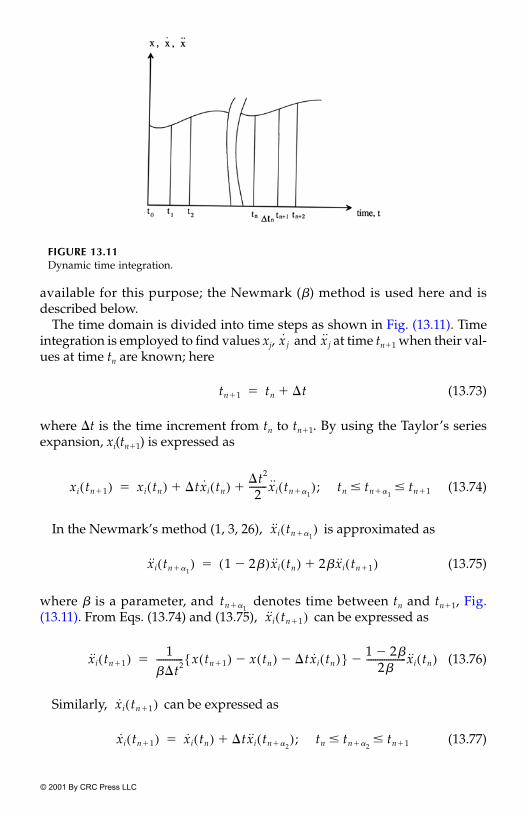
available for this purpose; the Newmark (�) method is used here and isdescribed below.
The time domain is divided into time steps as shown in Fig. (13.11). Timeintegration is employed to find values xj, and at time tn�1 when their val-ues at time tn are known; here
(13.73)
where �t is the time increment from tn to tn�1. By using the Taylor’s seriesexpansion, xi(tn�1) is expressed as
(13.74)
In the Newmark’s method (1, 3, 26), is approximated as
(13.75)
where � is a parameter, and denotes time between tn and tn�1, Fig.(13.11). From Eqs. (13.74) and (13.75), can be expressed as
(13.76)
Similarly, can be expressed as
(13.77)
FIGURE 13.11Dynamic time integration.
x j x j
tn�1 tn �t��
xi tn�1( ) xi tn( ) �txi tn( ) �t2
2-------- xi tn�1
( ); tn tn�1tn�1� �� ��
xi tn�1( )
xi tn�1( ) 1 2��( ) xi tn( ) 2� xi tn�1( )��
tn�1
xi tn�1( )
xi tn�1( ) 1��t2------------ x tn�1( ) x tn( )� �txi tn( )�{ } 1 2��
2�------------------ xi tn( )��
xi tn�1( )
xi tn�1( ) xi tn( ) �txi tn�2( ); tn tn�2
tn�1� ���
© 2001 By CRC Press LLC

and in Eq. (13.77) is approximated as
(13.78)
where � is another parameter, and is the intermediate time, Fig. (13.11).From Eqs. (13.77) and (13.78), can be expressed as
(13.79)
Substitution of Eqs. (13.76) and (13.79) into Eq. (13.72) yields
(13.80)
where
(13.81a)
(13.81b)
(13.81c)
In the above equations, the mass matrix Mij and damping matrix Cij are con-stant. For linear problems, stiffness Kij is constant and xi (tn�1) can be obtainedby solving Eq. (13.80). For nonlinear problems, the stiffness matrix Kij
depends on xi (tn�1), and iterative techniques such as Newton-Raphsonmethod have to be used to solve for xi (tn�1). After xi (tn�1) are found from Eq.(13.80), (tn�1) and (tn�1) may be found from Eqs. (13.76) and (13.79).
The stability of the Newmark’s scheme for linear systems has been investi-gated by many researchers and is expressed as (3, 26)
2� � � � 0.5 ----- unconditionally stable� � 0.5 ----- conditionally stable with the restriction on time
step given by
(13.82)
where � is the maximum natural frequency and � is the damping ratio of thesystem. This condition has to be satisfied for the maximum natural frequencyof the system. The recommended values of and � are 0.5 and 0.25, whichare found to yield stable results for the dynamic problems.
xi tn�2( )
xi tn�2( ) 1 ��( ) xi tn( ) � xi tn�1( )��
tn�2
xi tn�1( )
xi tn�1( ) xi tn( ) �t 1 ��( ) xi tn( ) � xi tn�1( )�{ }��
Kij�
xj tn�1( ) f ii
�
Kij� 1
��t2------------ Mij
���t---------- Cij Kij���
f i� f i tn�1( ) Mij
xj tn( )
��t2--------------
x j tn( )��t
-------------- 12�------- 1�
x j tn( )� �
��
Cij�
��t---------- xj tn( ) �
�--- 1�
x j tn( ) �2�------- 1�
�t x j tn( )� �
�
xi xi
��t �crit� � �12---�
�2--- � �
2�
12---�
2
��
12---
�2--- ��
----------------------------------------------------��
© 2001 By CRC Press LLC

13.5 Implementation
The dynamic Eqs. (13.66) can be written in matrix notation as (24, 25)
(13.83)
by denoting , and , Eq. (13.83)can be written as
(13.84)
Time integration with Eq. (13.84) using the Newmark �-method then leadsto
(13.85)
It usually requires iterative-incremental analysis to solve Eq. (13.85). Then, atiteration r, Eq. (13.85) can be written as
(13.86)
where is the increment of displacement during iteration, r, forincrement of load (displacement), n � 1. Now, Eq. (13.85) is written as
(13.87a)
where
(13.87b)
M˜
ac M˜
ad
M˜
bc M˜
bd
U˜˙ c
W˜˙ d
O
˜O˜
o˜
C˜
bd�
U˜˙ c
W˜˙ d
B˜ u
T�˜
a Vd
V
�
B˜ w
T pI˜
VdV
�
�Q˜
ua
Q˜
w
�
x˜˙ T U
˜˙ c
W˜˙[ ]� x
˜˙T U
˜˙ c
W˜˙ d[ ]� x
˜T U
˜c Wc[ ]�
M˜
x˜˙ C
˜x˜˙ K
˜x˜
� � Q˜
�
K˜
�x˜
tn�1( ) Q˜
�tn�1( )�
K�
˜x˜
r tn�1( ) dx˜
r tn�1( )�( ) Q� tn�1( )�
dx˜
r tn�1( )
K˜
�dx˜
r tn�1( ) Q˜
� tn�1( ) K˜
�x˜
� tn�1( )��
K˜
� 1��t2------------ M
˜�
��t---------- C
˜�
K˜
� ��
© 2001 By CRC Press LLC

and
(13.87c)
In Eq. (13.87), the mass and damping matrices are assumed toremain constant, and for nonlinear material behavior, the stiffness matrix varies and depends on displacement and pore pressure , through the con-stitutive matrix, , Eq. (13.12), as
(13.88)
Here we assumed that the strains in the RI, observed and FA parts are com-patible, and
(13.89)
where is the RI matrix, is the FA matrix and dD, the increment or rateof D, expressed as
(13.90)
The vector can be derived based on the given yield and disturbancefunctions. In the computer procedure, dD can also be evaluated as dD �D(tt+1) � D(tn).
Thus, and are constant and the tangent stiffness matrix, ,involves variations during the nonlinear behavior because is evaluatedas the tangent quantity.
13.6 Partially Saturated Systems
Computer (FE) procedures for partially saturated materials have been pro-posed by many investigators, based on constitutive models discussed inChapter 9. In a general and coupled formulation, displacements, fluid pres-sures, and suction are considered as independent variables. (See Referencesin Chapter 9, and 27–29.) Such coupled procedures can, however, be com-plex and involve significant computational effort. It is possible to develop
Q˜
�tn�1( ) Q
˜tn�1( ) M
˜
x˜
tn( ) x˜
r tn�1( )�
��t2----------------------------------------
x˜˙ tn( )��t------------ 1
2�------- 1�
x˜˙ tn( )� ���
C˜
� ���t---------- x tn( ) x
˜r tnH( )�( )
��--- 1�
x˜˙ tn( )
�2�------- 1�
�t x˜˙ tn( )� ��
M˜
( ) C˜
�( )K˜x
˜C˜
DSC
B˜
T�˜ n
ad Vd� �
B˜
TC˜
DSC qid Vd��
K˜
DSC qid�
C˜
DSC 1 D�( )C˜
i DC˜
c R˜
T�˜
c�˜
i�( )� ��
C˜
i C˜
c
dD R˜
T d�˜
i�
R˜
M˜
C˜
� K˜
�
K˜
DSC
© 2001 By CRC Press LLC
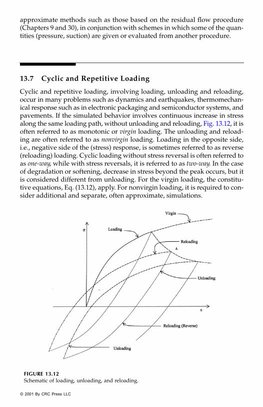
approximate methods such as those based on the residual flow procedure(Chapters 9 and 30), in conjunction with schemes in which some of the quan-tities (pressure, suction) are given or evaluated from another procedure.
13.7 Cyclic and Repetitive Loading
Cyclic and repetitive loading, involving loading, unloading and reloading,occur in many problems such as dynamics and earthquakes, thermomechan-ical response such as in electronic packaging and semiconductor systems, andpavements. If the simulated behavior involves continuous increase in stressalong the same loading path, without unloading and reloading, Fig. 13.12, it isoften referred to as monotonic or virgin loading. The unloading and reload-ing are often referred to as nonvirgin loading. Loading in the opposite side,i.e., negative side of the (stress) response, is sometimes referred to as reverse(reloading) loading. Cyclic loading without stress reversal is often referred toas one-way, while with stress reversals, it is referred to as two-way. In the caseof degradation or softening, decrease in stress beyond the peak occurs, but itis considered different from unloading. For the virgin loading, the constitu-tive equations, Eq. (13.12), apply. For nonvirgin loading, it is required to con-sider additional and separate, often approximate, simulations.
FIGURE 13.12Schematic of loading, unloading, and reloading.
© 2001 By CRC Press LLC

In the case of an elastoplastic model (e.g., HISS-�0), the simulated virginresponse allows for the effect of plastic strains and plastic hardening or yield-ing, Fig. 13.13(a). In the case of the softening behavior, the plasticity modelcan simulate the RI behavior, and the use of DSC allows for the degradation,Fig. 13.13(b).
Plastic deformations can occur during unloading and reloading, and caninfluence the overall response, Fig. 13.13. Although models to allow for suchbehavior have been proposed in the context of kinematic harding plasticity (31,32), they are often relatively complex and may involve computational difficul-ties. Hence, approximate schemes that are simple but can provide satisfactorysimulation have often been used; one such method is described below.
FIGURE 13.13Schematic of elastoplastic and softening (DSC) response.
© 2001 By CRC Press LLC

13.7.1 Unloading
As indicated in Fig. 13.12, the unloading response is often nonlinear. How-ever, as a simplification, it is often treated as linear elastic. Here, both linearand nonlinear elastic simulations are included. For the nonlinear case, ofwhich the linear simulation is a special case, the following procedure is used(24, 25). During unloading, the incremental stress-strain equation is given by
(13.91)
where is the elastic constitutive matrix with variable elastic unloadingmodulus, , Fig. 13.14, and the Poisson’s ratio, ν, is assumed to be constant.The modulus is given by
(13.92)
FIGURE 13.14Unloading interpolation function for CTC and SS tests (25).
d�˜
C˜
ULd�˜
�
C˜
UL
Eu
Eu
1Eu----- 1
Eb----- 1
Ep-----��
© 2001 By CRC Press LLC
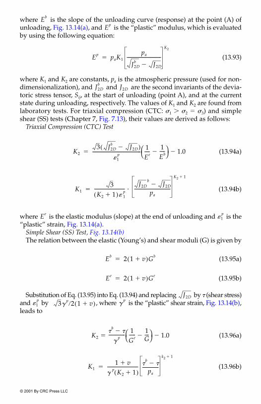
where is the slope of the unloading curve (response) at the point (A) ofunloading, Fig. 13.14(a), and is the “plastic” modulus, which is evaluatedby using the following equation:
(13.93)
where K1 and K2 are constants, pa is the atmospheric pressure (used for non-dimensionalization), and and are the second invariants of the devia-toric stress tensor, Sij, at the start of unloading (point A), and at the currentstate during unloading, respectively. The values of K1 and K2 are found fromlaboratory tests. For triaxial compression (CTC: �1 � �2 � �3) and simpleshear (SS) tests (Chapter 7, Fig. 7.13), their values are derived as follows:
Triaxial Compression (CTC) Test
(13.94a)
(13.94b)
where is the elastic modulus (slope) at the end of unloading and is the“plastic” strain, Fig. 13.14(a).
Simple Shear (SS) Test, Fig. 13.14(b)The relation between the elastic (Young’s) and shear moduli (G) is given by
(13.95a)
(13.95b)
Substitution of Eq. (13.95) into Eq. (13.94) and replacing by ! (shear stress)and by , where is the “plastic” shear strain, Fig. 13.14(b),leads to
(13.96a)
(13.96b)
Eb
Ep
Ep paK1pa
J2Db J2D�
-------------------------------
K2
�
J2Db J2D
K23 J2D
b J2D�( )�1
p--------------------------------------------
1Ee-----
1Eb-----�
1.0��
K13
K2 1�( )� 1p
----------------------------J2D
bJ2D�
pa---------------------------------
K2 1�
�
Ee�1
p
Eb 2 1 v�( )Gb�
Ee 2 1 v�( )Ge�
J2D
�1p
3�p 2 1 v�( ) �
p
K2!
b!�
�p
---------------�1
Ge------ 1
G----�
1.0�
K11 v�
�p K2 1�( )
---------------------------- !b
!�pa
---------------
k2 1�
�
© 2001 By CRC Press LLC

where and ! are the shear stresses at the point of unloading and duringunloading, respectively.
The values of and are evaluated by using the following equations:
(13.97a)
and
(13.97b)
13.7.2 Reloading
Figure 13.15 shows two cases of reloading, for the one-way and two-way. Inboth cases, the following constitutive equation is used:
(13.98)
where R is the interpolation parameter such that 0 � R � 1; R � 0 for thebeginning of reloading and R � 1 at the end of reloading. Thus, at the begin-ning of reloading, the behavior is elastic, given by
(13.99a)
At the end of reloading, virgin response resumes:
(13.99b)
The reloading elastic modulus, , for the two cases, Fig. 13.15, is different.For case 1, the elastic modulus at the start of reloading, , is given by
(13.100a)
where is the unloading slope at the beginning of unloading, Fig. 13.15(a).For case 2,
(13.100b)
where is the slope at the end of unloading, Fig. 13.15(b).
!b
�1p
�p
�1p 3 J2D
b
2------------------- 1
Ee-----
1Eb-----�
�
�p !
b
2---- 1
Ge------
1Gb------�
�
d�˜
a RC˜
DSCd�˜
1 R�( )C˜
ed�˜
��
d�˜
a C˜
ed�˜
�
d�˜
a C˜
DSCd�˜
�
ER
Ebr
Ebr Eb�
Eb
Ebr Ee�
Ee
© 2001 By CRC Press LLC

The interpolation parameter, R, for both cases is found as
(13.101)
where and are the second invariants of the stress tensor at the begin-ning of the last unloading and current level, respectively.
In computer (finite element) analysis, the reloading stress path may bebetween the above two cases. Then, a parameter, S, is defined as an indicatorof the direction of reloading:
(13.102)
where �1 � S � 1, , , and are the stress vectors before unloading, for thecurrent stress and for the next stress increment, respectively; S � �1 indicates
FIGURE 13.15Two reloading cases (25).
RJ2D
J2Db
-----------�
J2Db J2D
S�˜
b�˜
�( )Td�
˜� �
˜b
�˜
�( )T��d�˜
�-----------------------------------------�
�˜
b�˜
d�˜
© 2001 By CRC Press LLC

case 1 reloading, while S � 1 indicates case 2 reloading. Now, is interpo-lated between and E as
(13.103a)
Then, the modulus for reloading, , is found as
(13.103b)
where E is the elastic modulus of the material, which is often found as the (aver-age) slope of the line joining the unloading and end of unloading points or theinitial slope, Fig. 13.15(a). Then at the beginning of reloading when R � 0, �
, which ensures smooth transition from unloading to reloading, Fig.13.15(b). At the end of reloading (R � 1), � E, which ensures smooth tran-sition from reloading to the virgin loading.
13.7.3 Cyclic-Repetitive Hardening
In the case of elastoplastic behavior, there exists an in situ yield surface (F0) cor-responding to the initial or past state of stress experienced by the materialbefore the present cyclic or repetitive load is applied, Fig. 13.16. When unload-ing occurs, the plastic strains can change (increase or decrease), and hence, forthe reloading after the unloading, the yield surface that defines the elasticlimit usually expands from F0 to the initial surface, Fi, corresponding to eachcycle N (� 1, 2, …). As a result, the magnitudes of plastic strains decrease fromone cycle to the next, which is often referred to as cyclic hardening.
For a given load or stress (increment), the final or bounding surface, Fb, canbe defined by solving for the incremental equations, Eq. (13.13). In the case ofrepetitive loading under constant amplitude of load (stress), Fig. 13.16(b), themaximum load (Pmax) will be the amplitude of the load (stress). In the case ofcyclic (one-way) loading, Fig. 13.16(c), the bounding surface, Fb, wouldchange for each stress increase. Note that in this repetitive load analysis, thetime effects are not included.
Mroz et al. (31) proposed a model for cyclic hardening, which was adoptedby Bonaquist and Witczak (33) for materials in pavement structures. A similarand approximate (modified) method for cyclic hardening is presented below.
For the given load or stress increment, two bounding surfaces are defined,F0 and Fb, Fig. 13.16, and the corresponding hardening functions and param-eters are 0 and b, Eq. (7.11), and �0 and �b, respectively. Here, � denotes theaccumulated plastic strains or trajectory:
(13.104)
Ebr
Eb
1Ebr------- 1 S�
2Eb-------------- 1 S�
2Ee--------------��
ER
1ER------ 1 R�
Ebr--------------- R
E----��
ER
Ebr
ER
� �˜
pd( )T�˜
pd( )[ ]1 2��
© 2001 By CRC Press LLC

where is the vector of incremental plastic strains. Then the initial yieldsurface parameter, �i, for a given cycle, i, is expressed as
(13.105a)
where hc is the cyclic hardening parameter, determined from laboratoryrepetitive load tests. It controls the rate of expansion of the initial yield sur-face, Fi, at the end of unloading for a given cycle, N. If hc � 0, no cyclic hard-ening occurs. Bonaquist and Witczak (33) considered repeated tests involvingthe same stress (amplitude) to an initially unstrained material specimen with�0 � 0. Then, Eq. (13.105a) becomes
(13.105b)
FIGURE 13.16Cyclic hardening under repeated loading.
�˜
pd
�i �0 11
Nhc
--------� �b �0�( )��
� �b �i�1
Nhc
--------�b� �
© 2001 By CRC Press LLC

or
where � is the plastic strain trajectory up to cycle N. Plots of normalized tra-jectory � �b vs. number of cycles are used to find hc using a least square pro-cedure. For a granular material, hc � 1.06 was found (33).
With the above formulation, the value of �i, Eq. (13.105) is used to evaluatethe hardening function, i, Eq. (7.11). It is used to define the elastoplastic con-stitutive matrix � , Eq. (7.51), and the general DSC matrix ,Eq. (13.12), when reloading occurs.
13.8 Initial Conditions
In the foregoing algorithmic procedures, it is necessary to establish the initialconditions, which usually involve the location of the initial state (I) on theyield surface, F, Fig. 13.17a, for the RI response, and the initial disturbance,D0, Fig. 13.17b.
13.8.1 Initial Stress
The initial state of stress, , is often known from the in situ or residualstresses. We assume that the observed and RI stresses are initially equal, i.e.,
. The value of the initial hardening function, o, is found from Eq.(7.11) as (34)
(13.106)
where the subscript 0 denotes initial quantity. Thus, the initial state I on the yield surface, Fig. 13.17(a), is defined. The value of the initial plasticstrain trajectory, �0, can be found as
(13.107a)
If the initial state of stress is isotropic or hydrostatic, the foregoing equationsare simplified as
(13.108a)
��b---- 1
Nhc
--------�
Cep[ ] Ci[ ] CDSC[ ]
�˜
a
�˜ 0
i�˜ 0
a�
0 �J2D0
i
J10i2 1 �Sro�( ) 0.50�
-------------------------------------------�J10
i
pa------
2 n�
�
�˜ 0
i , 0( )
�0a1
o-----
1 �1
�
0 �J10
pa------
2 n�
�
© 2001 By CRC Press LLC

and
(13.108b)
and
(13.108c)
13.8.2 Initial Disturbance
It is usually difficult to define the initial disturbance, D0, due to effects suchas existing microcracking and anisotropy, and manufacturing defects. How-ever, it can be possible to quantify it on the basis of nondestructive measure-ments and/or mechanical testing.
Nondestructive ultrasonic velocities and attenuation can be measured indifferent directions in a laboratory test specimen. Such measurements for
FIGURE 13.17Initial state: hardening and disturbance.
�0 �v0 a0 0( )1 �1� �
�D 0�
© 2001 By CRC Press LLC
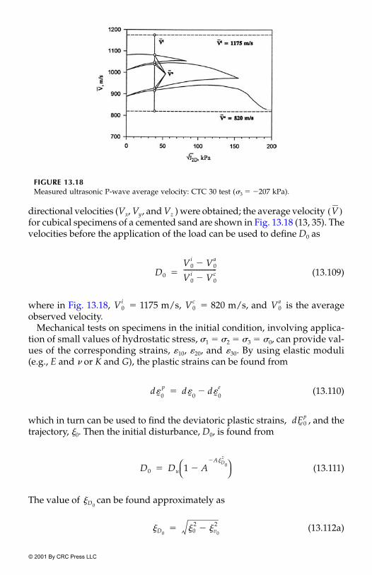
directional velocities (Vx, Vy, and Vz ) were obtained; the average velocity for cubical specimens of a cemented sand are shown in Fig. 13.18 (13, 35). Thevelocities before the application of the load can be used to define D0 as
(13.109)
where in Fig. 13.18, � 1175 m/s, � 820 m/s, and is the averageobserved velocity.
Mechanical tests on specimens in the initial condition, involving applica-tion of small values of hydrostatic stress, �1 � �2 � �3 � �0, can provide val-ues of the corresponding strains, �10, �20, and �30. By using elastic moduli(e.g., E and � or K and G), the plastic strains can be found from
(13.110)
which in turn can be used to find the deviatoric plastic strains, , and thetrajectory, �0. Then the initial disturbance, D0, is found from
(13.111)
The value of can be found approximately as
(13.112a)
FIGURE 13.18Measured ultrasonic P-wave average velocity: CTC 30 test (�3 � �207 kPa).
V( )
D0
V0i V0
a�
V0i V0
c�
---------------------�
V0i V0
c V0a
d�˜ 0
p d�˜ 0
d�˜ 0
e��
dE˜ 0
p
D0 Du 1 AA�D0
z�
� �
�D0
�D0�0
2�v0
2��
© 2001 By CRC Press LLC
where
(13.112b)
The values of , 0 and D0 are then used to define the constitutive matrix,, for the first load increment in Eq. (13.12). Then various quantities dur-
ing the incremental loading are found as
(13.113a)
(13.113b)
(13.113c)
(13.113d)
where N denotes the number of load increments.
13.9 Hierarchical Capabilities and Options
The DSC allows integrated and hierarchical capabilities to adopt, dependingupon specific need(s) and materials, models for various features such as elas-tic, plastic and creep responses, microcracking leading to fracture, degrada-tion and softening and stiffening or healing. Thus, if the general constitutivematrix, , Eq. (13.12), is developed, one can choose various hierarchicaloptions, depicted in Table 13.1.
The computer (FE) procedures with the DSC model can permit solutionsof problems with options for materials that are characterized as elastic, plas-tic, and creep, with inclusion of degradation and stiffening. For instance,Table 13.2 shows twelve such options available in the codes (8, 10, 25). It maybe noted that the user needs to provide input for only those parameters rele-vant for the specific hierarchical model chosen.
�V0
�0�Q��
˜
--------
3 �Q��
˜
-------- T �Q
��˜
--------
1 2-------------------------------------------�
�˜ 0
i
C˜ 0
DSC
�˜ n�1 �
˜ 0 d�˜ n�1
1
N
���
n�1 0 dn�11
N
���
�n�1 �0 d�n�11
N
���
Dn�1 D0 dDn�11
N
���
C˜
DSC
© 2001 By CRC Press LLC

TABLE 13.1
Hierarchical Options in DSC
TABLE 13.2
Various Options in the DSC and Parameters
Parameters
Model Elastic Plastic Creep DisturbanceThermal
Effects (T)�
1. Elastic (E) E, v 2. E(T)3. Elastoplastic classical
(ep c) e.g., von MisesE, v �y 4. ep c(T)
5. Elastoplastic hardening (ep h)
E, v �, �; n; a1, �1 6. ep h(T)
7. ep h with disturbance
E, v �, �; n; a1, �1 A, Z, Du 6. ep h(T)withdisturbance
9. Elastoviscoplastic�� E, v �, �; n; a1, �1 �, N 10. evp(T)11. Elastoviscoplastic
(evp) with disturbance��
E, v �, �; n; a1, �1 �, N A, Z, Du 12. evp(T) withdisturbance
�Thermal effects are included by expressing parameters as in Eq. (13.54).��Other creep overlay models (e.g., ve, vevp) (Chapter 8) are also available in the codes.�y � yield stress, T � temperature.
© 2001 By CRC Press LLC

13.10 Mesh Adaption Using DSC
Adaption of the finite element mesh during loading, and depending on thephysical state of the deforming material, has been one of the active areas ofrecent investigations. For the case of linear or nonlinear elastic and plastichardening materials when the problem is self-adjoint elliptic and the systemmatrices are positive definite, adaptive strategies such as those based onenergy norm are well established. However, for problems involving micro-cracking, localization, and softening or degradation, there does not appear toexist a global error norm similar to the energy norm for the self-adjoint ellip-tic problem (36). Hence, it becomes necessary to consider and develop criteriafor adaptive strategies based on other scalar variables (36–38). Zienkiewicz etal. (36) suggested definition of error (e) in terms of a scalar variable, �, as
(13.114)
where � is the exact solution and is the finite element solution; this defi-nition may, however, be difficult to implement, as the value of � is notknown. However, we can now use the scalar disturbance, D, in the DSC,which is computed and available as a part of incremental nonlinear analysis,to develop criteria for mesh adaptivity. In the following, we describe an adap-tive mesh procedure in which the traditional approach is used in the prepeakregion, while a disturbance-based procedure is used for the postpeak regionin which localization occurs and grows (39).
13.10.1 Prepeak Response
The uniform degree of error distribution (UDED) scheme proposed in (40) isused. Here, the error, e(i), is expressed as
(13.115)
where is the vector of computed stresses (from the displacement FE for-mulation), is the vector of “exact” stresses, and i denotes an element. Theexact stress, , is computed by using a hybrid FE procedure; details of theprocedure are given in (39, 41).
The strategy for generating a nearly optional mesh is based on the follow-ing criterion:
(13.116)
e � �h
��
�h
e i( ) abs�˜
� �˜
�
�˜
------------------
�
�˜ �
˜�
�˜
�
e e�
© 2001 By CRC Press LLC
where e is the computed error, Eq. (13.115), and is the permissible error, say,5%. The approximation error, em, in each element is given by
(13.117)
where m is the number of elements in the mesh, and � hmax is the normor maximum size of the element. The local mesh enrichment indicator, �, isgiven by
(13.118)
where is the energy norm for element i:
(13.119)
The element size (h) for the optimal mesh is evaluated as (40)
(13.120a)
where hi is the original maximum size of elements, and p is the order of inter-polation functions. For elements near singularities of order, k, the new ele-ment size is estimated from
(13.120b)
where k represents the strength of the singularly, which usually is adopted tobe equal to 0.50.
13.10.2 Postpeak Response
As stated earlier, the foregoing UDED scheme alone may not apply or is notsufficient for the postpeak region with localization. Here, the disturbance, D,Eq. (13.22) is used as the “error” indicator for mesh adaption. For example,critical values of disturbance, � 0.5, 0.75, or 0.90 can be specified as theindicator; that is, during the incremental analysis when the critical distur-bance, , is reached and exceeded, mesh refinement is initiated. As the dis-turbance is expressed in terms of plastic strain trajectory or dissipated energy,it represents the intensity of (strain) localization. Then, use of disturbance asthe remeshing indicator is consistent with the physical state of the structureundergoing microcracking and localization.
e
em e h m1 2�
h
�E i
em---------�
E i
E i e˜
i( )TC˜
1� e˜
i( ) VdV1��
hhi
�1 p
--------�
hhi
�1 k
--------�
D�
D�
© 2001 By CRC Press LLC

The error indicator in the postpeak region is given by
(13.121)
The error ratio for stress is given by
(13.122)
where e0 is the lowest error and ei is the error in any element. The mesh isrefined by using the following strategy:
(13.123)
where h0 is the size of the element with the lowest error, and t is the exponent;usually, t � 2.0 provides satisfactory results. Examples of adaptive meshingusing the above procedure are given in (39).
13.11 Examples of Applications
Typical problems involving computer analysis of factors such as localization,spurious mesh dependence, and stability are included in Chapter 12. Now,we describe solutions of a wide range of problems (civil, mechanical, elec-tronic packaging, pavements) obtained by using two- and three-dimensionalcomputer procedures with the DSC and its hierarchical versions (10, 25, 42).The computer predictions are compared with analytical, and from othernumerical procedures, and or laboratory and field behavior of practical engi-neering problems.
Example 13.1: Material Block: DSC Model, Effect of Load Increments
Figure 13.19(a) shows a one-element material (concrete) block, idealized asaxisymmetric, and subjected to the total vertical load of 80 MPa. The load isapplied in different incremental steps equal to 20, 50, and 100 (43). The mate-rial properties are given below (6, 44).
Elastic: E � 3.7 � 104 MPa, v � 0.25;Plasticity (HISS �0-Model): � � 0.06784, � � 0.75526, 3R � 47.5 MPa,
n � 5.23697, Disturbance: A � 668, Z � 1.50277, Du � 0.875
D D��
�e0
ei---------�
hi �th0
e0
ei---------
t
h0� �
a1 0.46 10 10� ,�1� 0.862;� �
© 2001 By CRC Press LLC

Figure 13.19(b) shows computed vertical stress ( � relative intact, and �observed or actual), and octahedral shear stress versus the axial strain
responses for the analyses with three different load steps. The simplifiedDSC scheme 3 was used for these calculations. It can be seen that the computed
FIGURE 13.19Effect of load steps or increments.
�yi
�ya
!octa( )
�y( )
© 2001 By CRC Press LLC

results are essentially the same from the analyses with three sizes of load steps,indicating the validity and robustness of the simplified solution scheme 3.
Example 13.2: Load (Footing) on Half Space (Soil): Elastoplastic(HISS-�1) Model
Computer algorithms for the finite element method and routines for the imple-mentation of the HISS-�0 and �1 models have been presented in (5, 34). The FEprocedure was used to predict the laboratory-measured stress and deformationbehavior of a circular footing on cohesionless material (Leighton Buzzard sand).
The material parameters for the sand were obtained from a comprehen-sive series of laboratory multiaxial and triaxial tests on cubical and cylindri-cal specimens under different initial confining pressures (�0 � �3) anddensities (5, 34). The elastic modulus, E, was considered to vary with depth(or �3) as (34)
(13.124)
where K is the modulus, is the modulus exponent and pa is the atmo-spheric pressure. The material parameters for the sand with relative densityDr � 95% were found by using procedures described in Chapters 4 to 7; theyare given below.*
Footing (steel)Elastic: E � 30 � psi (207 GPa), � � 0.30Soil:Elastic: K � 1256, � 0.70, � � 0.29;Plasticity (HISS �1-Model): � � 0.10212, � � 0.36242, n � 2.5;
a1 � 0.134575, �1 � 450.0, a2 � 0.0047,�2 � 1.02;
Nonassociative: " � 0.29Atmospheric Pressure: pa � 14.7 psi (101.35 kPa)In situ Stress Ratio: Ko � 0.5Unit Weight of Sand: � 0.10 lb/ (27.14 KN )
Here, the hardening () function is given by
(13.125)
The finite element mesh for the soil and circular footing (steel) is shown inFig. 13.20. It consists of 207 nodes and 58 eight-noded elements; 2 � 2 Gaussintegration was used. The total footing load of 25.0 psi (172 kPa) was appliedin steps of 2.50 psi (17 kPa), as it was done in the laboratory footing test (5).
* ©John Wiley & Sons Ltd. Reproduced with permission.
E K pa�3
pa-----
n�
n
106
n
� in3 m3
a1e�1��
1�D
a2 �2�D�------------------------�
�
© 2001 By CRC Press LLC

Figures 13.21 and 13.22 show comparisons between predicted and measureddisplacements at the center node (No. 15), and at a distance of 12.0 inches (30.0 cm)from the center of the footing (node 138), respectively. Figure 13.23 shows com-puted and measured vertical stress (�y) in the element under the footing. Thepredictions and measurements show satisfactory correlations.
FIGURE 13.20Finite elements mesh of soil-footing (1 in � 2.54 cm) (5, 34) (with permission from ElsevierScience and ©John Wiley & Sons Ltd; reproduced with permission).
FIGURE 13.21Load displacement response at center of footing (Node 15) (34). ©John Wiley & Sons Ltd.Reproduced with permission.
© 2001 By CRC Press LLC

Example 13.3: Layered (Pavement) System: Elasticity and Elastoplastic(HISS-�0) Models
Permanent deformation leading to rutting is one of the important distresses inthe analysis and design of highway and airport pavements (45, 46). The finiteelement procedure with various characterizations involving elastic and elasto-plastic (HISS-�0) models for different layers was used to analyze the develop-ment of deformations and stresses in a four-layered pavement system; thefinite element mesh, idealized as axisymmetric, is shown in Fig. 13.24.
FIGURE 13.22Load displacement response at 12 inches from center of footing (Node 138) (34). ©John Wiley& Sons Ltd. Reproduced with permission.
FIGURE 13.23Normal stress, �y under the footing (34). ©John Wiley & Sons Ltd. Reproduced with per-mission.
© 2001 By CRC Press LLC

Laboratory triaxial test data for asphalt (47) and for unbound materials(base, subbase, and subgrade) (33) were used to determine the elasticity andplasticity parameters for the �0-model; they are shown below.
The maximum load of 200 psi (1380 kPa) was applied in increments so asto simulate the wheel load over a radius of 10.0 inch (25.0 cm). A parametricstudy was performed to evaluate the influence of characterizing materialbehavior as nonlinear elastoplastic vs. linear elastic. Accordingly, the follow-ing combinations were considered (10, 43, 45, 46):
EEEE All four layers linear elastic,HEEE Pavement nonlinear (HISS-�0), other layers linear elastic,EHHH Pavement linear elastic, other layers nonlinear (HISS-�0),HHHH All layers nonlinear (HISS-�0).
Figures 13.25(a) and (b) show vertical, v, and horizontal (radial), u, displace-ments of the top surface for the final load (� 200 psi) for the four combinations.The results show satisfactory trends. They also indicate the influence of non-linear (elastoplastic) material response on the predictions. For example, the
FIGURE 13.24FE mesh for layered system: 1 in � 2.54 cm, 1 psi � 6.89 kPa.
Material Parameters for Asphalt Pavement System
Parameters Asphalt concrete1 Base2 Subbase2 Subgrade2
# 500000.0 psi 56532.85 17098.56 10013.17v 0.30 0.33 0.24 0.24� 0.1294 0.0633 0.0383 0.0296� 0.00 0.70 0.70 0.70n 2.40 5.24 4.63 5.26
1.23 � 10�6 2 � 10�8 3.6 � 10�6 1.2 � 10�6
1.944 1.231 0.532 0.778
1Based on tests by Witczak (47).2Based on tests by Bonaquist (33).
1�1
© 2001 By CRC Press LLC

maximum displacements from the plasticity (HHHH) case are about threetimes those from the elasticity (EEEE) case. It is believed that the elastoplastic(HISS) model can provide for realistic evaluation of permanent displace-ments (rutting) in pavement systems.
Example 13.4: Reinforced Earth: DSC and Elastoplastic (HISS-d1) Model
Various types of reinforcements such as fibers, nails and geogrids are used tostrengthen compacted soils for different construction systems. They repre-sent composite systems discussed in Chapter 10. The DSC model with the
FIGURE 13.25Displacements at top surface (43).
© 2001 By CRC Press LLC
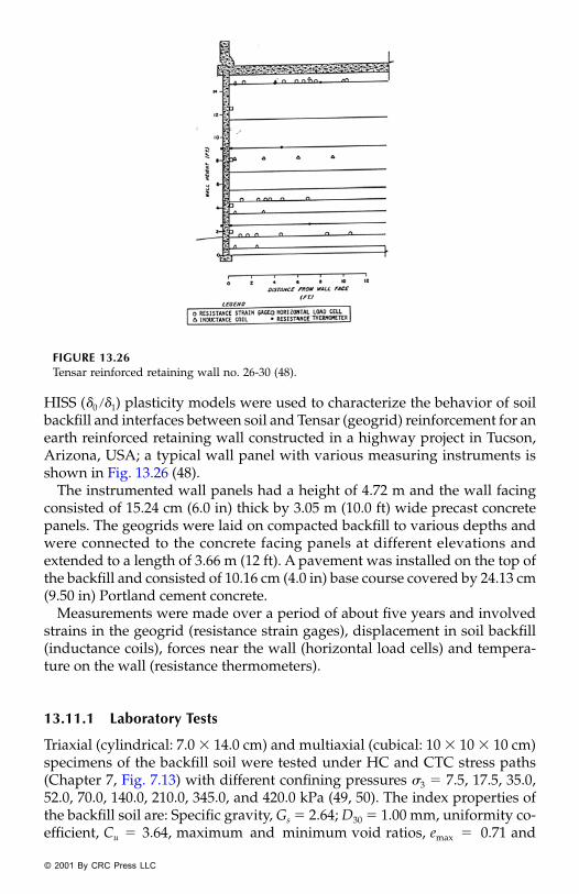
HISS (�0 �1) plasticity models were used to characterize the behavior of soilbackfill and interfaces between soil and Tensar (geogrid) reinforcement for anearth reinforced retaining wall constructed in a highway project in Tucson,Arizona, USA; a typical wall panel with various measuring instruments isshown in Fig. 13.26 (48).
The instrumented wall panels had a height of 4.72 m and the wall facingconsisted of 15.24 cm (6.0 in) thick by 3.05 m (10.0 ft) wide precast concretepanels. The geogrids were laid on compacted backfill to various depths andwere connected to the concrete facing panels at different elevations andextended to a length of 3.66 m (12 ft). A pavement was installed on the top ofthe backfill and consisted of 10.16 cm (4.0 in) base course covered by 24.13 cm(9.50 in) Portland cement concrete.
Measurements were made over a period of about five years and involvedstrains in the geogrid (resistance strain gages), displacement in soil backfill(inductance coils), forces near the wall (horizontal load cells) and tempera-ture on the wall (resistance thermometers).
13.11.1 Laboratory Tests
Triaxial (cylindrical: 7.0 � 14.0 cm) and multiaxial (cubical: 10 � 10 � 10 cm)specimens of the backfill soil were tested under HC and CTC stress paths(Chapter 7, Fig. 7.13) with different confining pressures �3 � 7.5, 17.5, 35.0,52.0, 70.0, 140.0, 210.0, 345.0, and 420.0 kPa (49, 50). The index properties ofthe backfill soil are: Specific gravity, Gs � 2.64; D30 � 1.00 mm, uniformity co-efficient, Cu � 3.64, maximum and minimum void ratios, emax � 0.71 and
FIGURE 13.26Tensar reinforced retaining wall no. 26-30 (48).
© 2001 By CRC Press LLC

emin � 0.37. The initial density of soil was about 17.3 kN/m3. Figures 13.27show typical test data for dry backfill under HC and CTC tests.
Interface shear tests between backfill and Tensar geogrid (16.00 cm diam)were conducted by using the CYMDOF device (Chapter 11) under different
FIGURE 13.27Typical stress-strain responses for backfill soil (49, 50).
© 2001 By CRC Press LLC

normal stresses, �n � 17.5, 35.0, 70.0, 140.0, 210.0, 350.0, 525.0, 700.0, 875.0,and 1050.0 kPa. Figures 13.28 show typical results for the normal loading,and shear loading (�n � 35.0 and 875.0 kPa) under displacement controlledcondition.
The test data was used to evaluate parameters for the DSC model for thesoil and interface by using procedures described in Chapters 7 and 11. Theparameters are shown below (49, 50).
Soil
Elastic: 61600 � , and � � 0.3;Plasticity: � � 0.12, � � 0.45, n � 2.56;Hardening: a1 � 3.0 � , �1 � 0.98, " � 0.20;
FIGURE 13.28Typical stress-strain responses for dry soil — Tensar geogrid interface.
�30.28
10 5�
© 2001 By CRC Press LLC

Disturbance: Du � 0.93, A � 0.368, Z � 1.60;Unit Weight � 18.84 KN/m3, co-efficient of earth pressure at rest, K0 � 0.40.
Interface
Elastic: Kn � 29100 � , Ks � 18350 � ;Plasticity: � � 2.3, � � 0.0, n � 2.8;Hardening: a1 � 0.03, �1 � 1.0, " � 0.40
As shown above, the elastic parameters E for soil, and normal andshear stiffness for interface, were found to be dependent on the confiningpressure, �3, and normal stress, �n, respectively. The DSC model wasused for the soil, while the HISS (�1) nonassociative model was used forinterfaces.
The material parameters for the soil above were obtained from the triaxialtests with cylindrical specimens. The volume change behavior was not avail-able from these tests; however, such behavior was available from the multiax-ial tests for the same soil. Hence, the multiaxial tests were back predicted asindependent tests. Figure 13.29 shows a typical comparisons between predic-tion and test data in terms of !oct and volumetric strain vs. axial strain for testwith �3 � 7.5 psi (52.0 kPa).
FIGURE 13.29Comparisons between predictions and multiaxial test data: �3 � 52.0 kPa (49, 50).
�n0.28
�n0.29
© 2001 By CRC Press LLC

The back predictions for the interface test were obtained by using the finiteelement code, DSC-SST2D (10). Figure 13.30 shows the finite element meshfor the test specimen: soil with 16.0 cm diam. and 4.00 cm height, and inter-face with 16.0 cm diam. and 0.15 height. The bottom nodes for soil wererestrained in the horizontal and vertical directions, while the side boundarieswere restrained in the horizontal direction. The nodes of the interface zonewere free to move. Typical comparisons between back predictions and testdata for �n � 35.0 and 875.0 kPa are shown in Fig. 13.31.
FIGURE 13.30FEM mesh for simulation of interface test.
FIGURE 13.31Comparisons between FE predictions and interface test data.
© 2001 By CRC Press LLC

13.11.2 Field Validation
The DSC-SST2D code (10) was used to predict the behavior of the Tensar-reinforced field wall, Fig. 13.26. The analyses were performed for two cases:Case 1, Fig. 13.32(a), involved a rather coarse mesh with three layers of Tensarreinforcement with interface elements, while for Case 2, a finer mesh with tenlayers of reinforcement was used; here, bar elements were used for the rein-forcement, and interface elements were provided on the top and bottom ofthe reinforcement, Fig. 13.32(b). In addition, interface elements were also pro-vided between the soil and wall for both cases.
The material parameters for the soil and interface were given previously.Parameters for the concrete wall facing and Tensar reinforcement, assumedto be linear elastic, are given below:
Wall Facing: E � 2.1 � kPa, � � 0.15
Reinforcement: E � 1.5 � 106 kPa.
The analysis involved simulation of excavation and embankment sequencesin which the Tensar reinforcement was placed sequentially on compactedbackfill layers. The traffic load was simulated by applying a load � 20 kPaon the top surface, after the end of construction. Typical results are givenbelow.
FIGURE 13.32Coarse and finer FE meshes for field Tensar reinforced wall (49, 50).
107
© 2001 By CRC Press LLC

FIGURE 13.32(continued).
© 2001 B
y CR
C P
ress LLC
© 2001 B
y CR
C P
ress LLC

Figure 13.33 shows comparisons between back predictions and field datafor vertical soil stress at the elevation 1.53 m (Fig. 13.26) after opening to traf-fic. These figures also show (the maximum) overburden pressure, �v � �h,where � is the density and h is the height. It can be seen that both Case 1 and2 results show good agreement with the field data. The vertical stress near thewall is lower, partly due to the soil-structure interaction and relative motionsat the interface. At a distance of about 1.52 m from the wall, the stress reachesmaximum value equal to the overburden stress.
Figure 13.34 shows comparisons between the predictions from Case 2 forthe horizontal soil stress in the elements near the inside wall face. It showsgood correlation, while the horizontal stress distribution using the classicalRankine theory exhibits much higher values compared to the observed
FIGURE 13.33Comparisons between predicted and observed vertical soil stress at elevation 1.53 m afteropening to traffic.
© 2001 By CRC Press LLC
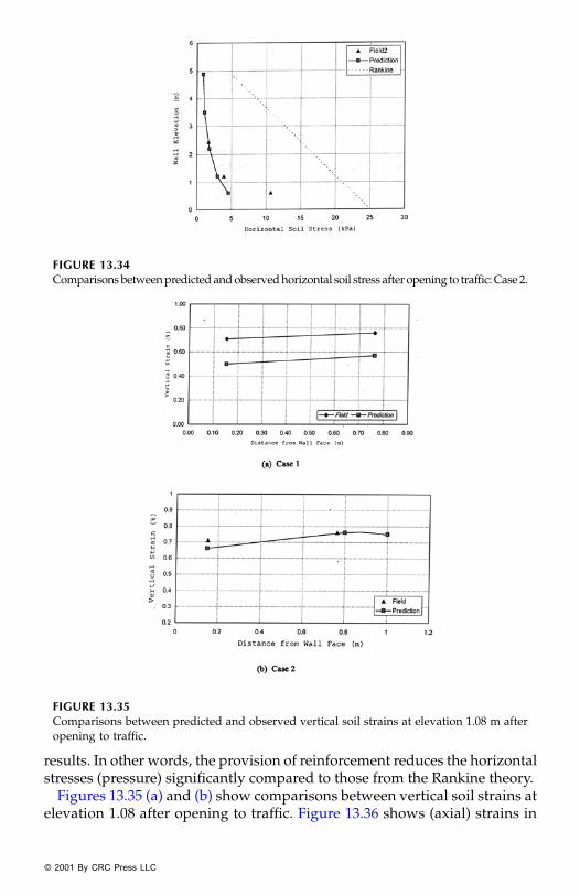
results. In other words, the provision of reinforcement reduces the horizontalstresses (pressure) significantly compared to those from the Rankine theory.
Figures 13.35 (a) and (b) show comparisons between vertical soil strains atelevation 1.08 after opening to traffic. Figure 13.36 shows (axial) strains in
FIGURE 13.34Comparisons between predicted and observed horizontal soil stress after opening to traffic: Case 2.
FIGURE 13.35Comparisons between predicted and observed vertical soil strains at elevation 1.08 m afteropening to traffic.
© 2001 By CRC Press LLC
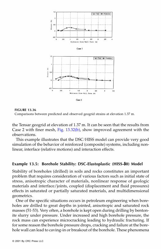
the Tensar geogrid at elevation of 1.37 m. It can be seen that the results fromCase 2 with finer mesh, Fig. 13.32(b), show improved agreement with theobservations.
This example illustrates that the DSC HISS model can provide very goodsimulation of the behavior of reinforced (composite) systems, including non-linear, interface (relative motions) and interaction effects.
Example 13.5: Borehole Stability: DSC-Elastoplastic (HISS-δδδδ0) Model
Stability of boreholes (drilled) in soils and rocks constitutes an importantproblem that requires consideration of various factors such as initial state ofstress, anisotropic character of materials, nonlinear response of geologicmaterials and interface/joints, coupled (displacement and fluid pressures)effects in saturated or partially saturated materials, and multidimensionalgeometrics.
One of the specific situations occurs in petroleum engineering when bore-holes are drilled to great depths in jointed, anisotropic and saturated rockmasses (51-53). Very often, a borehole is kept open during drilling by benton-ite slurry under pressure. Under increased and high borehole pressure, therock mass can experience microcracking leading to hydraulic fracturing. Iffor some reason the borehole pressure drops, cracking and failure at the bore-hole wall can lead to caving-in or breakout of the borehole. These phenomena
FIGURE 13.36Comparisons between predicted and observed geogrid strains at elevation 1.37 m.
© 2001 By CRC Press LLC
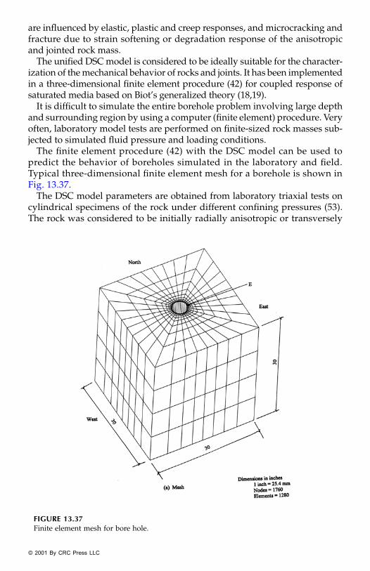
are influenced by elastic, plastic and creep responses, and microcracking andfracture due to strain softening or degradation response of the anisotropicand jointed rock mass.
The unified DSC model is considered to be ideally suitable for the character-ization of the mechanical behavior of rocks and joints. It has been implementedin a three-dimensional finite element procedure (42) for coupled response ofsaturated media based on Biot’s generalized theory (18,19).
It is difficult to simulate the entire borehole problem involving large depthand surrounding region by using a computer (finite element) procedure. Veryoften, laboratory model tests are performed on finite-sized rock masses sub-jected to simulated fluid pressure and loading conditions.
The finite element procedure (42) with the DSC model can be used topredict the behavior of boreholes simulated in the laboratory and field.Typical three-dimensional finite element mesh for a borehole is shown inFig. 13.37.
The DSC model parameters are obtained from laboratory triaxial tests oncylindrical specimens of the rock under different confining pressures (53).The rock was considered to be initially radially anisotropic or transversely
FIGURE 13.37Finite element mesh for bore hole.
© 2001 By CRC Press LLC

isotropic; the elastic stress-strain relation is given by (53, 54)
(13.126)
where E1 and E2 are elastic moduli, G12 is the shear modulus, and �12 and �23
are the Poisson’s ratios. These elastic parameters were expressed as func-tions of the mean pressure, p � �3 � J1/3, where �3 � confining stress andJ1 � �1 � �2 � �3:
(13.127)
The parameters for the HISS-�0 plasticity model used are given below.
� � 5.80, � � 0.60, n � 4.84,R � 67.0 psi (460 kPa),a1 � 1.14 � , �1 � 2.56.
In order to allow for failure condition at low mean pressures, the yield func-tion in the HISS-�0 model (Chapter 7) was modified as
(13.128)
where the exponent, q, allows for the nonlinearity of the ultimate yield func-tion (55); the value of (q) was found to be 1.4. Figure 13.38(a) shows thecurved ultimate envelopes, Eq. (13.128) for tests with loading in the paralleland normal directions. Figure 13.38(b) shows the plot of D vs. �D.
�1
�2
�3
�12
�23
�31
1E1-----
�21
E2------�
�21
E2------� 0 0 0
�12
E1------�
1E2-----
�23
E2------� 0 0 0
�12
E1------�
�23
E2------�
1E2----- 0 0 0
0 0 0 1G12-------- 0 0
0 0 0 0 1G23-------- 0
0 0 0 0 0 1G12--------
�1
�2
�3
!12
!23
!31
��
E1 E10
E1S E10�( )kE1J1
kE1J1 E1S E10��--------------------------------------------��
E2 E20E2S E20�( )kE2J1
kE2J1 E2S E20��-------------------------------------------- E10 at J1� 0� �
v1 v10v1S v10�( )kv1J1
kv1J1 v1S v10��------------------------------------------ E1s at J1� $� �
v2 v20
v2S v20�( )kv2J1
kv2J1 v2S v20��------------------------------------------��
10 17�
F J2D J1n
� �J1q
�( ) 1 �Sr�( ) 0.5�� 0� �
© 2 0 0 1 B y C R C P r e s s L L C

FIGURE 13.38Nonlinear ultimate envelope and disturbance.
© 2001 B
y CR
C P
ress LLC
© 2001 B
y CR
C P
ress LLC

In the DSC model, the response of the fully adjusted part was characterizedby using the following equation:
(13.129)
where c denotes FA (critical) state. The parameter m was found to be 0.28.The disturbance parameters, Eq. (3.16), used are as follows:
A � 74 � 104
Z � 2.265Du � 0.999.
Figure 13.38b shows a plot of disturbance vs. �D.
13.11.3 Computer Results
The 3-D finite element mesh is shown in Fig. 13.37. Figure 13.39 shows pre-dicted E-W and N-S displacements with the pressure applied on the bore-hole. These results show consistent trends as observed in laboratory tests.The predictions of the pressure at the breakout, when large displacementsoccur, are considered to be realistic.
The growth of disturbance in element E, Fig. 13.37, in the E-W direction isalso plotted in Fig. 13.39. It shows that the critical disturbance, Dc ≈ 0.80, isreached between pressures of 3000 to 3500 psi (21 to 24 MPa). Thus, the insta-bility and breakout can be identified in the finite element analysis based onthe critical disturbance derived from laboratory tests.
FIGURE 13.38(continued).
J2Dc mJ1
c�
© 2001 By CRC Press LLC

FIGURE 13.39Predicted displacements and disturbance for borehole: 1 inch � 2.54 cm, 1 psi � 6.89 kPa.
© 2001 B
y CR
C P
ress LLC
© 2001 B
y CR
C P
ress LLC

Example 13.6: Viscoplastic Model: Cylinder (Tunnel) with Internal Pressure
Figure 13.40 shows the finite element mesh for a thick cylinder (tunnel), idealizedas plane strain; because of the symmetry, only a quarter of the cylinder is dis-cretized (56). The internal diameter of the cylinder is 100 mm, with wall thickness� 100 mm. It is subjected to internal pressure, P, equal to 14 N mm2. The materialparameters for the viscoplastic (�0-HISS) model (10) and those used by Owenand Hinton (17) in their viscoplastic (von Mises) model are given below:
Elastic: E � 2.10 � 103 N mm2, � � 0.3;von Mises: �y (yield stress) � 2.40 N mm2,
FIGURE 13.40Mesh for elastoviscoplastic problem (17) (with permission).
© 2001 By CRC Press LLC

H� (strain hardening parameter) � 0.00;HISS-�0: � � 0.05, � � 0.62, n � 3.9,
a1 � , �1 � 0.47, R � 2.0 N mm2;Creep: � � 0.01 1 day, N � 1.00.
Time Integration (Chapter 8):
Factor for graded time � 0.05Steppping time increment factor � 1.50
Time integration parameter, � � 0.0.
Figure 13.41(a) shows radial (x) displacement with time for node 1,obtained by using the viscoplastic (von Mises) model. The displacement con-verges to the value of 0.13997, which compares well with that of 0.13959reported by Owen and Hinton (17). Figure 13.41(b) shows the radial (x) dis-placement for node 1 with time obtained by using the viscoplastic (HISS-�0)model. The converged value of displacement of 0.160 mm is somewhathigher than that from the von Mises model, Fig. 13.41(a). The difference canbe due to the fact that in the HISS-�0 model, plastic yielding is incorporatedfrom the beginning of loading.
Viscoplastic Model: Creeping Natural Slope. Natural slopes oftenexhibit continuous movements under gravity load, which are influenced bycreep or viscous response of (geologic) materials in the slopes and the inter-face zone between the slope (solid body), and parent rock mass. Finite ele-ment analysis and comparisons between predictions and field observation ina natural slope at Villarbeney, Switzerland, are presented in (57–59).
Example 13.7: Layered Pavement System: DSC Model, Microcrackingand Fracture
Figure 13.42 shows the finite element mesh for a two-layered system with 4.0in (10.0 cm) thickness of pavement over a 42 in (107 cm) thick base (60). It wasidealized as axisymmetric. Two analyses were performed: (1) without initialcrack and (2) with an initial vertical crack (starting from the surface) of depth0.5 inch (1.27 cm) and thickness of 0.05 inch (0.127 cm) at the end of the circu-lar loaded area of 12.0 inch (30 cm) radius (10). The load was applied in (vari-able) increments [4 at 50 psi (350 kPa), 10 at 20 psi (140 kPa) and theremainder at 10 psi (70 kPa)] until failure, when the displacements becameexcessive (10, 45, 46).
The material in the pavement was characterized by using the DSC modelthat allows for elastoplastic response with disturbance (damage) leading tomicrocracking and fracture. The base material was characterized by usingthe elastoplastic HISS-�0 model. The material parameters are shown below.The crack region was assumed to be linear elastic with a very low value (100
10 9�
© 2001 By CRC Press LLC

psi � 0.69 MPa) of the elastic modulus (E). Before the load was applied, insitu stresses due to the (overburden) weight were computed and included inthe analysis using the unit weights and K0 values shown below.
Figure 13.43 shows the computed load displacement curves from the no-crack and crack analyses; it shows that the system with the crack is less stiffcompared to that without a crack, and that the initiation of yielding andmicrocracking occurred at lower load in the case of the crack.
FIGURE 13.41Radial displacement vs. time: viscoplastic model.
© 2001 By CRC Press LLC

Computed distributions and contours of disturbance (in a part of the pave-ment, near the applied load) at different load levels for the two cases (nocrack and with crack) were analyzed. For the case without an initial crack,critical disturbance Dc � 0.80 indicating initiation of fracture occurs at theinterface between the pavement and the base (under the load), at the load
FIGURE 13.42Typical mesh for layered pavement (1.0 inch � 2.54 cm).
Material Parameters.
Parameter
Material 1: Pavement(Concrete)
Material 2: Base Crack
Elastic
E psi (MPa) 3 � (20684) 3 � (2068) 100 (0.69)v 0.25 0.24 0.24
Plasticity (HISS-�0) model
� 0.0678 0.030� 0.755 0.700n 5.24 5.26a1 4.61 � 1.20 �
0.826 0.778R, psi (MPa) 8122 (56) 28.88 (0.20)A 668Z 1.502Du 0.875
In situ stress
Unit weight lb in.3
(kg )0.087 (2325) 0.064 (1771)
Co-efficient of lateral Earth pressure, Ko
0.20 0.70
106 105
10 11� 10 6�
�1
m3
© 2001 By CRC Press LLC

level of about 480 psi (3.30 MPa). At about 550 psi (3.80 MPa) load, Dc � 0.80is exceeded in almost all of the pavement under the load. In the case of theinitial crack, the critical disturbance Dc � 0.80 is indicated at the interface,and in the upper part (near the surface) of the cracked region at about 450 psi(3.10 MPa) load. As the load increases, the extent of zones with D � 0.8increases, and at about 490 psi (3.38 MPa) load, the entire pavement (belowthe load) experiences microcracking and fracture.
The above results show the capability of the DSC model for predictingmicrocracking and growth of fracture (in a layered system). Note that thenonlinear FE with the DSC allows for the identification of the initiation andgrowth of cracking, without the need for the introduction of linear fracturemechanics based crack intensity factors, and it avoids the need for the a prioriassumption of the location and geometry of the crack. In other words, theDSC identifies cracking and its propagation at locations dictated by thenature of the problem (geometry, loading, boundary conditions, etc.)
Example 13.8: Chip Substrate 313-PIN PBGA: DSC Model, Thermomechanical Cyclic Fatigue Failure
The DSC model has been used to characterize the thermomechanical behav-ior of joining materials (e.g., solders) in chip-substrate systems in electronicpackaging. The computer finite element codes with the DSC model havebeen used to analyze thermomechanical response of a number of chip-sub-strate systems: leadless ceramic chip carrier (LCCC) (7, 8, 14), ceramic ball
FIGURE 13.43Computed load displacement curves.
© 2001 By CRC Press LLC

grid array (CBGA) (61, 62), plastic ball grid array (PBGA) (63–66) and thinsmall outline package (TSOP) (9). The computer predictions for these prob-lems compared very well with laboratory test responses in terms of distur-bance (damage), microcracking and fracture, and cycles to failure. Twotypical problems are presented here; 313-Pin PBGA in this example and theCBGA in the next example.
Figure 13.44 shows the 313-PIN plastic ball grid array (PBGA) manufacturedby AMKOR–ANAM, which is 35.0 mm square and 2.33 mm high. The solderball diameter varies from 0.60 to 0.90 mm with the spacing of 1.27 mm. ThePBGA package was tested in the laboratory under thermal cycles of loading atthe Jet Propulsion Lab (JPL) (67). The PBGA module consisted of bimaleimidetriazine (BT) epoxy glass laminate, mold compound, silicon chip, bond wiresand micro solder balls. It is mounted on a printed wire board (PWB) composedof FR-4 glass epoxy laminated with copper traces or planes (63).
The analysis was performed in two stages: macro and micro. In the macromodel, the package was idealized as three-dimensional with linear elasticproperties, Fig. 13.45; the PBGA and PWB were divided in 144, 4-node planestrain plate elements each, and were connected by 84-bar elements to representthe solder joints in the quarter of the system. The thicknesses used correspond
FIGURE 13.44313-PBGA package (63, 67).
FIGURE 13.45PBGA PWB solder joint NASTRAN model (63).
© 2001 By CRC Press LLC

to the photomicrographs of the test hardware (63, 64). Other details such asboundary conditions and loading are given by Zwick and Desai (63, 64). Themacro model provided displacements at each nodal point and stresses ineach element. The highest displacements occurred in the solder joint farthestfrom the neutral point (package center) at temperature � �55�C.
Figure 13.46(a) shows the temperature and displacement cycles with thehighest magnitude applied for the analysis of a single ball joint, Fig. 13.46(b),in the micro model. The material parameters for the Pb-Sn solder are givenbelow (14, 63, 64). They were determined on the basis of test data on Pb Sn(40 60) solders reported in (68–71). At this time, the analysis involved elasto-plastic disturbance model, i.e., creep effects, are not considered.
The finite element analysis was performed for about 4000 cycles. Figure 13.47(a)shows the computed values of stresses �x, �y and !xy in the top left corner element,up to 2000 cycles. Cyclic degradation is evident in this figure. Figure 13.47(b)shows the growth of disturbance with cycles (N). Figure 13.48 shows the con-tours of disturbance at typical cycles N � 2500 and 2700 cycles.
Different values of design disturbance (Dcm), when microcracking isconsidered to initiate, can be specified for specific design needs. Forinstance, if Dcm � 0.50, the critical value (Dcm � 0.5) occurred in the solderafter about 500 cycles, Fig. 13.49. Then it grew with cycles, and after about3000 cycles (to failure, Nf), about 90% of the solder volume had experi-enced D � 0.50, Fig. 13.49, which can be considered to represent fatiguefailure. Alternatively, Dcm � Dc � 0.85, which represents the critical valuefrom laboratory tests (8, 14, 63), when significant fracture occurs as a con-sequence of the coalescence of microcracks, can be adopted as the designcriterion. It occurred for the first time after about 2000 cycles; then about10% of the solder volume reached D � 0.85 after about 2800 cycles (Nf),
Parameters for 63 Sn 37 Pb Solder (63)
Parameter P300 c(*)
ElasticityE 15.7 GPa �4.1� 0.40 0.0
Plasticity� 0.00081 �0.1579a1 0.78E-05 0.00η1 0.46 0.23n 2.10 0R 208.0 MPa �5.34
DisturbanceA 0.102 1.55Z 0.676 0Du 0.85 —
(*)Temperature effects are included by expressing anyparameter, P, as in Eq. (13.54).
© 2001 By CRC Press LLC

Fig. 13.49, which can be considered to be failure. Thus, cycles to failure(Nf) can be found based on a given design criterion on the disturbance, D.Figure 13.49 shows that the foregoing values of cycles to failure comparewell with those observed in the laboratory tests on the four PBGA 313-PINpackages (67).
FIGURE 13.46Displacement and temperature loading cycles and single ball micro model (63).
© 2001 By CRC Press LLC

Inclusion of creep behavior with elastoplastic disturbance model can pro-vide improved results. Also, the computer code can be used to perform para-metric studies in which the material properties, geometry, ball spacing, etc.,can be varied, leading to computation of cycles to failure and reliability, anddesign optimization (72).
Example 13.9: Chip Substrate CBGA Package: DSC Model, Thermomechanical Cyclic Fatigue Failure
Figure 13.50 shows a ceramic ball grid array (CBGA) package tested in the lab-oratory by Guo et al. (73). It is used in the IBM 604 power PC chip and is com-posed of either alumina or aluminum nitride (ALN), which encases a
FIGURE 13.47Stress variation and disturbance with cycles (63).
© 2001 By CRC Press LLC

controlled collapsible chip connection (C-4) silicon chip. The solder balls inthe CBGA-SBC (solder ball connect) package were composed of 90 10(Pb Sn) with 63 37 (Pb Sn) solder fillers. Details are given in (73, 74).
The material properties for the chip, printed wire board (PWB) and thejoining solder with 63% Pb-37% Sn and 90% Pb-10% Sn were determined on
FIGURE 13.48Contours of disturbance at cycles N � 2500 and 2750 (63).
FIGURE 13.49Disturbance and fractional volume vs. cycles and comparison with test data (63).
FIGURE 13.50Test vehicle for CBGA in simulated laboratory test (61).
© 2001 By CRC Press LLC

the basis of laboratory tests and other data available in (75–77). These param-eters are given below (61).
The solder materials were characterized by using the DSC with elastoplas-tic �0-model for the RI behavior; the FA response was assumed to be hydro-static. The chip and PWB material were assumed to be linear elastic. A seriesof tension and compression tests were performed on ALN so as to determineits elastic constants (8, 61).
The finite element analyses were performed by considering three differentball spacings, 1.00, 1.27, and 1.50 mm; they involved two steps: macro andmicro. In the macro level, half of the structure was idealized as plane strain;Figure 13.51 shows the FE mesh with 4-node isoparametric elements for thecase of 1.27 mm spacing. The mesh consisted of 360 nodes and 304 elements.In the macro model, a thermal cycle, Fig. 13.52(a), was applied and the criti-cally strained solder ball was identified. Figure 13.52(b) shows displacementcycles with computed (critical) amplitudes of axial and shear displacementsthat were applied in the analysis of the single ball for the micro level calcula-tions. Figure 13.53 depicts the finite element mesh for the single ball.
Figure 13.54 shows the computed axial (normal) and shear displacementsfor different ball spacings, together with the experimental data (73) andanother finite element analysis for the same package reported by Corbin (74).
Material Parameters
63% Pb-37% Sn 90% Pb-10% Sn Parameter P300 c P300 c
ElasticityE 15.7 GPa �4.1 9.29 GPa �1.92� 0.40 0.0 0.40 0.0
Plasticity� 0.00081 �0.158 0.000822 �0.16a1 0.78 � 0.00 1.10 � 10�5 �0.61�1 0.46 0.23 0.44 0.24n 2.10 0.00 2.10 0.00R 208.0 MPA �5.34 122.0 MPA �1.67
DisturbanceA 0.102 1.55 4.07 0.00Z 0.676 0.0 1.95 0.00Du 0.90 0.0 0.90 0.00
CeramicModule
E 318 GPa� 0.23r 7.0 � �C
PWB (FR-4)E 11.0 GPa� 0.28r 20 � �C
Here, P300 and c are parameters in Eq. (13.54)
10 5�
10 6�
10 6�
© 2001 By CRC Press LLC

The present results show satisfactory correlation with the test data andCorbin’s analysis. A part of the difference can be attributed to the fact that thesize of the module analyzed here is smaller than that used by Corbin (74) andin the testing. Also, in the present analysis, the structure analyzed was 21 �21 mm, while Corbin considered a 25 � 25 mm SBC module (8, 61). In thepresent analysis, a two-dimensional plain strain idealization was used, whileCorbin considered a three-dimensional idealization. Furthermore, the molyb-denum and copper pads at the top and bottom of the ball were not included inthe present analysis; this was done as a simplification, and because failure usu-ally initiates in the filler, not in the pads.
Disturbance (microcracking leading to fracture) growth and its localizationwith thermal cycles were computed for the three ball spacings. Figure 13.53
FIGURE 13.51Typical finite element mesh for ball spacing � 1.27 mm (61).
FIGURE 13.52Thermal cycles and applied displacements: from macromodel applied to micromodel forball spacing � 1.27 mm (8,61). ©1998 IEEE.
© 2001 By CRC Press LLC

shows typical distributions of computed disturbance for the ball spacing of1.27 mm at cycles N � 100, 500 and Nf � 873; here, Nf denotes failure cycle,which corresponded to the critical disturbance, Dc � 0.90. Figure 13.53shows that at Nf � 873, the growth of D � 0.90 has extended to the major partof the package, for about 80 to 90% of the width of the ball. This can be con-sidered to represent failure, as the finite crack for about 80 to 90% of thewidth could lead to failure of the electrical connection. The distributions ofdisturbance, which represent accumulated plastic strains in Fig. 13.53, com-pare well with those reported from interferometry results (73) and the finiteelement analysis (74).
FIGURE 13.53Finite element mesh and distribution of disturbance in solder ball for 1.27 at different thermalcycles, N (8, 61). ©1998 IEEE.
© 2001 By CRC Press LLC

Figure 13.55 shows a plot of the number of cycles to failure, Nf, vs. the viaspacing. It can be seen that the values of Nf decrease as the spacing increases.In other words, a package with a smaller ball spacing can sustain a greaternumber of thermal and mechanical cycles. The DSC model and computerprocedure can thus also allow design optimization and evaluation of reliabil-ity under variations of factors such as ball spacing, material properties,geometry and loading cycles (rate, dwell, etc.) (72).
Example 13.10: Cyclic Hardening, Repetitive Loading, HISS Plasticity(�0) Model
Figure 13.56 shows the finite element mesh with four 8-noded elements. Thetop surface was subjected to cyclic or repetitive pressure loading with theamplitude of 50.0 MPa, increased in twenty increments and then decreased
FIGURE 13.54Computed displacements and comparisons with previous FE analysis (74) and test data(73). ©1993 by IBM Corp., reprinted with permission.
© 2001 By CRC Press LLC

to zero in twenty decrements. Five such cycles were applied in the presentanalysis (10, 56). The material parameters used are given below:
Elastic: E � 37000 MPa, � � 0.25;Plasticity (HISS-�0) Model: � � 0.06784, � � 0.755, n � 5.24;
a1 � 0.4614 � , �1 � 0.826,
3R = 56.64 MPaFor the nonlinear unloading, Fig. 13.14, � 50,000 MPa and � 35,000MPa were used. The values of the cyclic hardening parameter, hc, Eq.(13.105a), were adopted as 0.00 and 1.00.
Three cases were analyzed: (1) hc � 0.00 indicating no cyclic hardeningand with linear unloading, (2) hc � 1.00 indicating cyclic hardening and withlinear unloading, and (3) hc � 1.0 indicating cyclic hardening and with linearunloading, Fig. 13.14.
Figure 13.57 shows computed results for the three cases in terms of axialstress (�y) versus axial strain (�y) for the five cycles. Figure 13.57(a) shows thatthere is no cyclic hardening, as the plastic strains for all cycles are the same.The results for cases 2 and 3, Fig. 13.57(b) and (c), show that the plastic strainsdecrease with increasing cycles. However, Case 3 can allow the effect of non-linear unloading on the observed behavior of some materials.
FIGURE 13.55Plot of the number of cycles to failure vs. via spacing for three ball spacings (8, 61). ©1998IEEE.
10 10�
Eb Ee
© 2001 By CRC Press LLC

Example 13.11: Pile in Clay under Cyclic Loading: DSC Model
Interaction and coupled response between structures and geologic materialsplay an important role in the behavior of structure-foundation systems. Thebehavior is complex and affected by many factors such as nonlinearresponse of soils and interfaces, type of loading and sequences of construc-tion. The finite element procedure with the DSC model was used to predictthe field behavior of an instrumented axially loaded pile in saturated marineclay (23–25, 78–82).
The pile load tests were performed by Earth Technology Corporation (78) atSabine, Texas, with pile segments of diameter 4.37 cm and 7.62 cm. Typicalanalysis for the 7.62 cm pile is presented below. The field conditions includingin situ stresses and sequences—pile driving, consolidation, tension (one-way)tests and cyclic two-way loading—were simulated. The in situ stresses, beforethe pile was driven, were computed by using the coefficient of lateral earthpressure, Ko � 0.786 (23). The driving stresses and pore water pressures wereevaluated by using the strain path method (SPM) (23, 79, 83). The drivingstresses and pore water pressures were introduced as “initial” conditions for
FIGURE 13.56Four-element mesh and repeated loading.
© 2001 By CRC Press LLC

FIGURE 13.57Computed cycles stress, �y vs. strain, .�y
© 2001 By CRC Press LLC
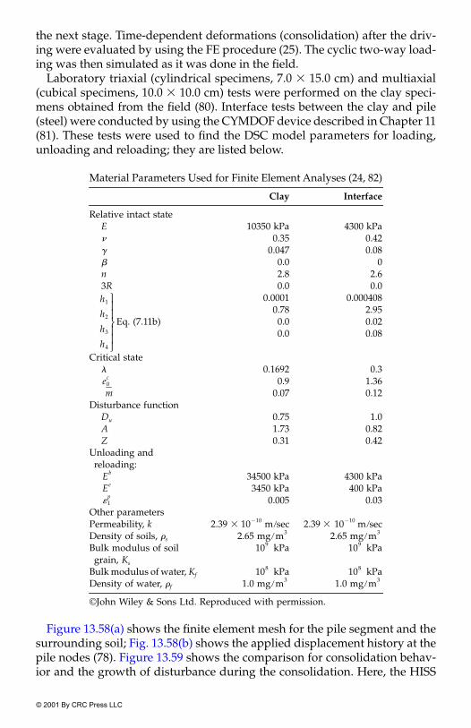
the next stage. Time-dependent deformations (consolidation) after the driv-ing were evaluated by using the FE procedure (25). The cyclic two-way load-ing was then simulated as it was done in the field.
Laboratory triaxial (cylindrical specimens, 7.0 � 15.0 cm) and multiaxial(cubical specimens, 10.0 � 10.0 cm) tests were performed on the clay speci-mens obtained from the field (80). Interface tests between the clay and pile(steel) were conducted by using the CYMDOF device described in Chapter 11(81). These tests were used to find the DSC model parameters for loading,unloading and reloading; they are listed below.
Figure 13.58(a) shows the finite element mesh for the pile segment and thesurrounding soil; Fig. 13.58(b) shows the applied displacement history at thepile nodes (78). Figure 13.59 shows the comparison for consolidation behav-ior and the growth of disturbance during the consolidation. Here, the HISS
Material Parameters Used for Finite Element Analyses (24, 82)
Clay Interface
Relative intact stateE 10350 kPa 4300 kPa� 0.35 0.42� 0.047 0.08� 0.0 0n 2.8 2.63R 0.0 0.0
Eq. (7.11b)
0.0001 0.0004080.78 2.95
0.0 0.020.0 0.08
Critical state� 0.1692 0.3
0.9 1.36 0.07 0.12
Disturbance functionDu 0.75 1.0A 1.73 0.82Z 0.31 0.42
Unloading and reloading:
34500 kPa 4300 kPa3450 kPa 400 kPa
0.005 0.03Other parametersPermeability, k 2.39 � m sec 2.39 � m secDensity of soils, �s 2.65 mg 2.65 mg
Bulk modulus of soil grain, Ks
kPa kPa
Bulk modulus of water, Kf kPa kPaDensity of water, �f 1.0 mg 1.0 mg
©John Wiley & Sons Ltd. Reproduced with permission.
h1
h2
h3
h4
e0c
m
Eb
Ee
�1p
10 10� 10 10�
m3 m3
109 109
108 108
m3 m3
© 2001 By CRC Press LLC

indicates calculations based on previous anisotropic hardening HISSplasticity model (23, 79). Figures 13.60(a) and (b) show comparisons betweenthe predicted responses using the DSC and HISS model and the fielddata for shear transfer at the pile interface vs. displacement and time duringthe one-way cyclic loading, respectively. The pore water pressure and thegrowth of disturbance vs. time during the one-way cyclic loading are shownin Figs. 13.60(c) and (d), respectively. The results for the cyclic two-way load-
FIGURE 13.58Finite element mesh of field pile test and displacement history (24, 82). ©John Wiley & SonsLtd. Reproduced with permission.
�0�( )
�0�( )
© 2001 By CRC Press LLC

ings in terms of shear transfer vs. displacement, shear transfer vs. time, porewater pressures and growth of disturbance vs. time are shown in Figs.13.61(a)–(d), respectively.
It can be seen that the DSC predictions correlate very well with field observa-tions. Also, the DSC model, which allows for cyclic (disturbance) degradation,provides improved predictions compared to those from the HISS-plasticitymodel.
Example 13.12: Dynamic Analysis and Liquefaction in Shake Table Test:DSC Model
Behavior of structure foundation systems subjected to dynamic (earth-quake) loading is affected, among other factors, by interaction effects dueto relative interface motions. In the case of saturated granular (sandy)materials with certain initial densities, dynamic loading can cause micro-structural instability or liquefaction (Chapter 9). Applications of computerprocedures with the DSC model are given in (84–88). The DSC parametersfor the Ottawa sand and sand-concrete (steel) interfaces were obtainedfrom cyclic triaxial and multiaxial (84, 85, 88, 89) and shear tests (90),respectively. Here, we present dynamic and liquefaction analysis of ashake table test (91).
FIGURE 13.59Comparisons between field consolidation behavior and predicted results from HISS andDSC models (24, 82). ©John Wiley & Sons Ltd. Reproduced with permission.
© 2001 By CRC Press LLC

The finite element procedure with the DSC model was used to predictthe dynamic behavior in shake table tests reported by Akiyoshi et al. (91).Figure 13.62(a) shows the shake table test set-up with location of instruments.The saturated sand was Fuji River sand with total density, �t � 19.8 KN m3.Here, the properties of the Ottawa sand with �t � 19.63 KN m3 were used asan approximation; the rationale for the approximation is given in (85).
The finite element mesh used is shown in Fig. 13.62(b). The mesh contained160 elements and 190 nodes with 120 elements for the soil and 40 elements forthe steel box. The concept of repeating side boundaries was used (21, 92);accordingly, the displacement of the side boundary nodes on the same horizon-tal plane was assumed to be the same. The bottom boundary was restrained inthe vertical direction, while it was free to move in the horizontal direction.
The applied loading involved horizontal displacement, X, at the bottomnodes, given by the following function:
(13.130)
where is amplitude (� 0.0013 m), f is the frequency (� 5.0 HZ) and t is thetime. The analysis was carried out for 50 cycles with time step �t � 0.001
FIGURE 13.60Comparisons between field measurements and predictions from DSC and HISS models:one-way cyclic load test (24, 82). ©John Wiley & Sons Ltd. Reproduced with permission.
X x 2%f t( )sin�
x
© 2001 By CRC Press LLC

sec (from time 0.0 to 2.0 secs), and �t � 0.05 sec (from time 2.0 to 10.0secs).
Figure 13.63 shows comparisons between the measured and predicted excesspore water pressures with time at the (dark) point in the box at depth � 300 mmfrom the top, Fig. 13.62(b). The test results indicate liquefaction after about 2.0secs when the pore water pressure equaled the initial effective stress. The finiteelement predictions also show liquefaction after about 2.0 secs.
Figures 13.64(a) to (d) show contours and growth of disturbance in themesh at typical times = 0.50, 1.0, 2.0, and 10.0 secs. The computed plot ofthe growth of disturbance at depth � 300 mm is shown in Fig. 13.64(e).Laboratory tests on the Ottawa sand showed that liquefaction initiated ataverage critical disturbance, Dc � 0.84 (87). At time � 0.50 sec, the distur-bance was below the critical value in all elements. At t � 1.0 sec, the distur-bance had grown and its value was greater than 0.70 in the middle zone,including depth � 300 mm. At time of 2.0 secs, the disturbance had reachedthe value of about 0.80 in the zone above depth � 300 mm, while its value
FIGURE 13.60(continued).
© 2001 By CRC Press LLC

was greater than 0.80 in the lower middle zone, indicating that liquefactionhad initiated at about 2.0 secs. At time � 10.0 secs, the disturbance has grownto the value of about 0.90 in about 80% of the test box, indicating that the soilin the test box has liquefied and failed. These trends are considered to be con-sistent with the observed behavior.
13.12 Computer Codes
A number of computer codes with the DSC model have been developed andare used to solve the problems in this chapter. Some of the codes aredescribed in various publications, e.g., DSC-SST2D (10), DSC-DYN2D (25)and DSC-SST3D (42). These codes can be acquired by writing to the author.
FIGURE 13.61Comparisons between field measurements and predictions from DSC and HISS models:two-way cyclic load test (24, 82). ©John Wiley & Sons Ltd. Reproduced with permission.
© 2001 By CRC Press LLC

References
1. Desai, C. S. and Abel, J. F., Introduction to the Finite Element Method, VanNostrand Reinhold, New York, 1972.
2. Zienkiewicz, O. C., The Finite Element Method, 3rd Edition, McGraw Hill,London, UK, 1997.
3. Bathe, K. J., Finite Element Procedures, Prentice-Hall, Englewood Cliffs, NJ, 1996. 4. Desai, C. S. and Kundu, T., Introductory Finite Element Method, CRC Press, Boca
Raton, FL, 1999, under publication. 5. Desai, C. S. and Hashmi, Q., “Analysis, Evaluation and Implementation of a
Nonassociative Model for Geologic Materials,” Int. J. Plasticity, 5, 1989, 397–420. 6. Desai, C. S. and Woo, L., “Damage Model and Implementation in Nonlinear
Dynamic Problems,” Int. J. Comp. Mechanics, 11, 2 3, 1993, 189–206.
FIGURE 13.61(continued)
© 2001 By CRC Press LLC

7 Basaran, C., Desai, C. S. and Kundu, T., “Thermomechanical Response of Ma-terials and Interfaces in Electronic Packaging: Parts I and II,” J. of Electron.Packaging, 120, 1, 1998, 41–47, 48–53.
8. Desai, C.S., Basaran, C., Dishongh, T. and Prince, J. L., “ThermomechanicalAnalysis in Electronic Packaging with Unified Constitutive Model for Materialsand Joints,” IEEE Trans.: Components, Packaging and Manuf. Tech., Part B, 21, 1,1998, 87–97.
9. Desai, C. S., Wang, Z. and Whitenack, R., “Unified Disturbed State ConstitutiveModels for Materials and Computer Implementation,” Keynote Paper, 4th Int.Conf. on Constitutive Laws for Engineering Materials, Rensselaer Polytechnic Inst.,Troy, NY, 1999.
FIGURE 13.62Shake table and finite element mesh (85). (a) ©John Wiley & Sons Ltd. Reproduced withpermission.
© 2001 By CRC Press LLC

10. C. Desai, “DSC-SST2D-Computer Code for Static, Dynamic, Creep and ThermalAnalysis: Solid, Structure and Soil-Structure Problems,” Reports and Manuals,Tucson, AZ, 2000.
11. Wang, Z. and Desai, C. S., “Modelling and Computer Thermomechanical Anal-ysis of Problems Using the Disturbed State Concept,” Report, under publication,1999.
12. Kachanov, L. M., Introduction to Continuum Damage Mechanics, Martinus Nijhoft,Dorchrecht, The Netherlands, 1986.
13. Desai, C. S. and Toth, J., “Disturbed State Constitutive Modeling Based onStress-Strain and Nondestructive Behavior,” Int. J. Solids Struct., 33, 11, 1996,1619–1650.
14. Desai, C. S., Chia, J., Kundu, T. and Prince, J., “Thermomechanical Responseof Materials and Interfaces in Electronic Packaging: Parts I and II,” J. of ElectronicPackaging, 119, 1997, 294–305.
15. Prager, W., “Nonisothermal Plastic Deformations,” Bol. Koninke Nederl. Acad.Wet, 8, 6113, 1958, 176–182.
16. Perzyna, P., “Fundamental Problems in Viscoplasticity,” in Advances in AppliedMechanics, Academic Press, New York, 1996, 244–368.
17. Owen, D. R. and Hinton, E., Finite Elements in Plasticity: Theory and Practice,Pineridge Press, Swansea, UK, 1980.
18. Biot, M. A., “General Solutions of the Equations of Elasticity and Consolidationfor a Porous Material,” J. Appl. Mech., 23, 1956, 91–96.
19. Biot, M. A., “Mechanics of Deformation and Acoustic Propagation in PorousMedia,” J. Appl. Physics, 33, 4, 1962, 1482–1498.
20. Sandhu, R. S. and Wilson, E. L., “Finite Element Analysis of Flow of SaturatedPorous Elastic Media,” J. of Eng. Mech. Div., ASCE, 95, 3, 1969, 641–642.
FIGURE 13.63Excess pore presure at depth of 300 mm (85).
© 2001 By CRC Press LLC
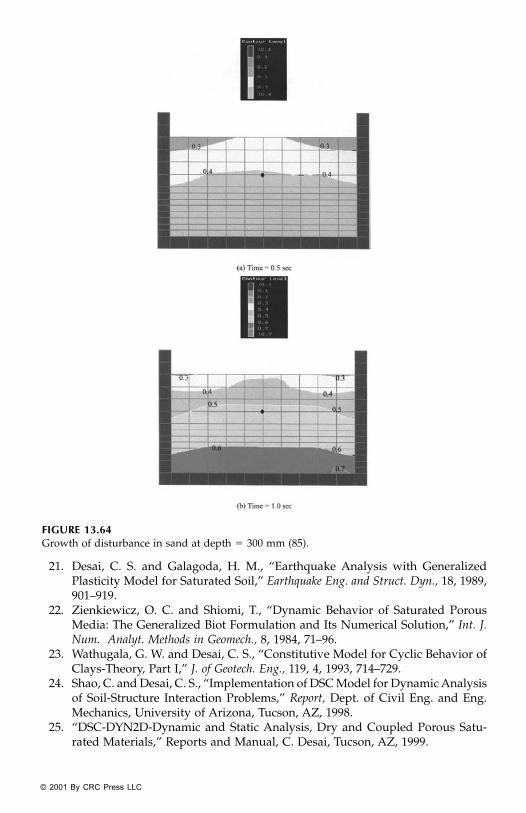
21. Desai, C. S. and Galagoda, H. M., “Earthquake Analysis with GeneralizedPlasticity Model for Saturated Soil,” Earthquake Eng. and Struct. Dyn., 18, 1989,901–919.
22. Zienkiewicz, O. C. and Shiomi, T., “Dynamic Behavior of Saturated PorousMedia: The Generalized Biot Formulation and Its Numerical Solution,” Int. J.Num. Analyt. Methods in Geomech., 8, 1984, 71–96.
23. Wathugala, G. W. and Desai, C. S., “Constitutive Model for Cyclic Behavior ofClays-Theory, Part I,” J. of Geotech. Eng., 119, 4, 1993, 714–729.
24. Shao, C. and Desai, C. S., “Implementation of DSC Model for Dynamic Analysisof Soil-Structure Interaction Problems,” Report, Dept. of Civil Eng. and Eng.Mechanics, University of Arizona, Tucson, AZ, 1998.
25. “DSC-DYN2D-Dynamic and Static Analysis, Dry and Coupled Porous Satu-rated Materials,” Reports and Manual, C. Desai, Tucson, AZ, 1999.
FIGURE 13.64Growth of disturbance in sand at depth � 300 mm (85).
© 2001 By CRC Press LLC

26. Hughes, T. J. R., “Analysis of Transient Algorithms with Particular Referenceto Stability Behavior,” Chapter in Computational Methods for Transient Analysis,Belytschko, T. and Hughes, T. J. R. (Editors), North-Holland Publ. Co., Amster-dam, 1983.
27. Thomas, H. R. and He, Y., “Analysis of Coupled Heat, Moisture and Air Trans-fer in a Deformable Unsaturated Soil,” Geotechnique, 45, 4, 1995, 677–689.
28. Thomas, H. R. and Li, C. L. W., “Modelling Transient Heat and MoistureTransfer in Unsaturated Soil Using a Parallel Computing Approach,” Int. J.Num. and Analyt. Methods in Geomech., 19, 1996, 345–366.
29. Yang, D. Q., Rahardjo, H., Leong, E.C. and Choa, V., “Coupled Model for Heat,Mositure, Air Flow and Deformation Problems in Unsaturated Soils,” J. of Eng.Mech., ASCE, Vol. 124, No. 12, 1998, 1331–1338.
30. Ng, A. K. L. and Small, J. C., “Coupled Finite Element Analysis for UnsaturatedSoils,” Int. J. Num. Analyt. Meth. in Geomech., in press, 1999.
FIGURE 13.64(continued)
© 2001 By CRC Press LLC

31. Mroz, Z., Norris, V. A. and Zienkiewicz, O. C., “An Anisotropic HardeningModel for Soils and Its Application to Cyclic Loading,” Int. J. Num. Analyt.Methods in Geomechanics, 2, 1978, 203–221.
32. Somasundaram, S. and Desai, C. S., “Modeling and Testing for AnisotropicBehavior of Soils,” J. of Eng. Mech., ASCE, 114, 9, 1988, 1473–1497.
33. Bonaquist, R. F. and Witczak, M. W., “A Comprehensive Constitutive Modelfor Granular Materials in Flexible Pavement Structures,” Proc., 8th Int. Conf. onAsphalt Pavements, Seattle, WA, 1997, 783–802.
34. Desai, C. S., Sharma, K. G., Wathugala, G. W. and Rigby, D. B., “Implementationof Hierarchical Single Surface �0 and �1 Models in Finite Element Procedure,”Int. J. Num. Analyt. Meth. in Geomech., 15, 1991, 649–680.
35. Desai, C. S., Jagannath, S. V. and Kundu, T., “Mechanical and Ultrasonic Aniso-tropic Response of Soil,” J. of Eng. Mech., ASCE, 121, 6, 1995, 744–752.
36. Zienkiewicz, O. C., Huang, M. and Pastor, M., “Localization Problems in Plas-ticity Using Finite Elements with Adaptive Remeshing,” Int. J. Num. and Analyt.Meth. Geomechanics, 19, 2, 1995, 127–148.
37. Yu, J., Peric, D. and Owen, D. R. J., “Adaptive Finite Element Analysis of aStrain Localization Problem for the Elasto-Plastic Cosserat Continuum,” in Com-putational Plasticity III: Models, Software and Applications, Owen, D. R. J. et al.(Editors), Pineridge Press, Swansea, 1992, 551–566.
38. Belytschko, T. and Tabbara, M., “H-Adaptive Finite Element Methods for Dy-namic Problems with Emphasis on Localization,” Int. J. Numer. Methods Eng.,36, 1993, 4245–4265.
39. Desai, C. S. and Zhang, W., “Computational Aspects of Disturbed State Con-stitutive Models,” Int. J. Comput. Methods in Applied Mechanics and Engineering,151, 1998, 361–376.
40. Zienkiewicz, O. C. and Zhu, J. Z., “A Simple Error Estimator and AdaptiveProcedure for Practical Engineering Problems,” Int. J. Numer. Meth. Eng., 24, 2,1987, 337–357.
FIGURE 13.64(continued)
© 2001 By CRC Press LLC

41. Zhang, W. and Chen, D. P., “The Patch Test Conditions and Some MultivariantFinite Element Formulations,” Int. J. Numer. Methods Eng., 40, 16, 1997,3015–3032.
42. Desai, C., “DSC-SST3D-Computer Code for Static and Coupled Dynamic Anal-ysis: Solid (Porous) Structure and Soil-Structure Problems,” Reports and Man-ual, Tucson, AZ, 1999.
43. Wang, Z., Private communication, 1999.44. Frantziskonis, G. and Desai, C. S., “Constitutive Model with Strain Softening,”
Int. J. Solids Struct., 23, 6, 1987, 733–750.45. Desai, C. S., “Review and Evaluation of Models for Pavement Materials,”
Report, Tucson, AZ, 1999.46. Desai, C. S., “Unified Disturbed State Constitutive Model for Asphalt Con-
crete,” Proc., 14th Eng. Mech. Conference, ASCE, Austin, TX, May 2000.47. Witczak, M. W., “The Universal Airport Pavement Design System: Report II.
Asphalt Mixture Material Characterization,” The University of Maryland, Col-lege Park, MD, 1989.
48. Fishman, K. L., Desai, C. S. and Sogge, R. L., “Field-Behavior of InstrumentedGeogrid Soil Reinforced Wall,” J. of Geotech. Eng., ASCE, 119, 8, 1993, 1293–1307.
49. El-Hoseiny, K. and Desai, C. S., “Material and Interface Modeling and Com-puter Analysis of Instrumented Geogrid Soil Reinforced Wall,” Interim Report,University of Arizona, Tucson, AZ, 1999.
50. El-Hoseiny, K., “Soil Stabilization Using Geosynthetics,” Ph.D. Thesis, Univ. ofMenoufia, Menoufia, Egypt, 1999.
51. Desai, C. S. and Reese, L. C., “Stress Deformation and Stability Analysis ofDeep Boreholes,” Proc., 2nd Congress, Int. Soc. for Rock Mech., Belgrade, Yugo-slavia, 1970.
52. Desai, C. S. and Johnson, L. D., “Influence of Bedding Planes on Stability ofBoreholes,” Proc., 3rd Congress, Int. Soc. of Rock Mechs., Denver, CO, 1974.
53. Desai, C., “Finite Element 3-D Procedure with the Disturbed State Model forWellbore Stability,” Report, Tucson, AZ, 1999.
54. Niandou, H., Shao, J. F., Henry, J. P. and Fourmaintraux, D., “LaboratoryInvestigation of the Mechanical Behaviour of Tournemire State,” Int. J. RockMech. Min. Sc., 34, 1, 1997, 3–16.
55. Desai, C. S. and Ma, Y., “Modelling of Joints and Interfaces Using the DisturbedState Concept,” Int. J. Solids and Struct., 16, 1992, 623–653.
56. Sharma, K. G., Private communication, 1998.57. Desai, C. S., Samtani, N. C. and Vulliet, L., “Constitutive Modeling and Analysis
of Creeping Slopes,” J. of Geotech. Eng., ASCE, 121, 1, 1995, 43–56.58. Samtani, N. C., Desai, C. S. and Vulliet, L., “An Interface Model to Describe
Viscoplastic Behavior,” Int. J. Num. Analyt. Meth. Geomech., 20, 1996, 231–252.59. Vulliet, L., “Modelisation des Pentes Naturelles en Mouvement,” Thesis No.
635, Ecole Polytechnique Federale de Lausanne, Lausanne, Switzerland, 1986.60. Cohen, D., Private communication, 1998.61. Dishongh, T. J. and Desai, C. S., “Disturbed State Concept of Materials and
Interfaces with Applications in Electronic Packaging,” Report to NSF, Dept. ofCivil Engng. and Engng. Mechs., University of Arizona, Tucson, AZ, 1996.
62. Dishongh, T. J. and Desai, C. S., “Calibration of the Disturbed State Model forThermomechanical Behavior of Various Solders,” Proc., Interpack 99, Hawaii,1999.
© 2001 By CRC Press LLC
63. Zwick, J. W., “Thermostructural Analysis of a 313-PIN Plastic Ball Grid Array(PBGA),” Report for M.E., Dept. of Civil Eng. and Eng. Mechanics, Universityof Arizona, Tucson, AZ, 1998.
64. Zwick, J. W. and Desai, C. S., “Structural Reliability of PBGA Solder Joints withthe Disturbed State Concept,” Proc., Interpack 99, Hawaii, 1999.
65. Desai, C. S., “Review and Evaluation of Approaches for ThermomechanicalAnalysis for Stress, Failure and Reliability,” Proc., Interpack 99, Hawaii, 1999.
66. Desai, C. S. and Whitenack, R., “Review of Models and the Disturbed StateConcept for Thermomechanical Analysis in Electronic Packaging,” J. of Elec-tronic Packaging, ASME, 123, 1–15, 2001.
67. Ghaffarian, R., “Ball Grid Array Packaging RTOP: Interim Environmental TestResults,” Jet Propulsion Lab, Cal Tech, Pasadena, CA, 1997.
68. Riemer, H. S., “Prediction of Temperature Cycling Life for SMT Solder Jointson TCE-Mismatched Substrates,” Proc., IEEE Electron. Comp., 1990, 418–423.
69. Skipor, A., Harren, S. and Bostis, J., “Constitutive Characterization of 63 37Sn Pb Eutectic Solder Using the Bodner-Parton Unified Creep-Plasticity Model,”Proc., Joint ASME/JSME Conf. Electron. Packag., Chen, W.T. and Abe, H. (Eds),2, 1992, 661–672.
70. Solomon, H. D., “Isothermal Fatigue of LCCC PWB Interconnections,” J. Elec-tron. Packag., ASME, 114, 1992, 161–168.
71. Pan, T. Y., “Thermal Cyclic Induced Plastic Deformations in Solder Joints – Part I:Accumulated Deformation in Surface Mount Joints,” Trans., ASME, 113, 1991, 8–15.
72. Whitenack, R. and Desai, C. S., “Computer Procedure with Disturbed StateModel for Cyclic Fatigue, Design and Reliability,” Report, under preparation,1999.
73. Guo, Y., Kim, C. K., Chen, W. T. and Woychik, C. G., “Solder Ball Connect (SBC)Assemblies under Thermal Loading: I. Deformation Measurements via MoireInterferometry and Its Interpretation,” IBM J. Res., Develop., 37, 5, 1993, 635–647.
74. Corbin, J. S., “Finite Element Analysis for Solder Ball Connect (SBC) StructuralDesign Optimization,” IBM J. Res. Develop., 37, 5, 1993, 585–596.
75. Cole, M., Caufield, T., Banks, D., Winton, M., Walsh, A. and Gonya, S., “Con-stant Strain Rate Tensile Properties of Various Load Based Solder Alloys at 0,50 and 100�C,” Proc., Microelectron. Packag. Conf., Montreal, P.Q., Canada, 1991.
76. Savage, E. and Getzan, G., “Mechanical Behavior of 60 Tin 40 Lead Solder atVarious Strain Rates and Temperatures,” Proc., Int. Soc. Hybrid Microelectron.(ISHM), Nashville, TN, 1990.
77. Nir, N., Duddear, T. D., Wang, C. C. and Storm, A. R., “Fatigue Properties ofMicroelectronic Solder Joints,” J. Electron. Packag., ASME, 113, 1999.
78. Earth Technology Corporation, “Pile Segment Tests, Sabine Pass: Some Aspectsof the Fundamental Behavior of Axially Loaded Piles in Clay Soils,” ETC ReportNo. 85-007, Houston, Long Beach, CA, 1986.
79. Desai, C. S., Wathugala, G. W. and Matlock, H., “Constitutive Model for CyclicBehavior of Clay, II: Application,” J. of Geotech. Eng., ASCE, 119, 4, 1993, 730–748.
80. Katti, D. R. and Desai, C. S., “Modeling and Testing of Cohesive Soils Usingthe Disturbed State Concept,” J. of Eng. Mech., ASCE, 21, 1995, 648–658.
81. Desai, C. S. and Rigby, D. B., “Cyclic Interface and Joint Shear Decising Includ-ing Pore Pressure Effects,” J. of Geotech. & Geoenv. Eng., ASCE, 123, 1997,568–579.
© 2001 By CRC Press LLC

82. Shao, C. and Desai, C. S., “Implementation of DSC Model and Application forAnalysis of Field Pile Tests Under Cyclic Loading,” Int. J. Num. Analyt. Meth.Geomech., 24, 6, 2000, 601–624.
83. Baligh, M. M., “Undrained Deep Penetration, I: Shear Stresses; Part II: PorePressures,” Geotechnique, 36, 1986, 471–485, 487–501.
84. Park, I. J. and Desai, C. S., “Disturbed State Modeling for Dynamic and Liq-uefaction Analysis,” Report to NSF, Dept. of Civil Engng. and Engng. Mechs.,University of Arizona, Tucson, AZ, 1997.
85. Park, I. J. and Desai, C. S., “Cyclic Behavior and Liquefaction of Sand UsingDisturbed State Concept,” J. of Geotech. and Geoenv. Eng., ASCE, 126, 9, 2000.
86. Desai, C. S., “Soil-Structure Analysis of Foundations with Unified ConstitutiveModels for Soils and Interfaces,” Proc., Analysis, Design and Construction, andTesting of Deep Foundations, OTRC Conference, University of Texas, Austin, TX,ASCE, April 1999.
87. Desai, C. S., Park, I. J. and Shao, C., “Fundamental Yet Simplified Model forLiquefaction Instability,” Int. J. Num. Analyt. Meth. Geomech., 22, 1998, 721–748.
88. Desai, C. S., “Evaluation of Liquefaction Using Disturbed State and EnergyApproaches,” J. of Geotech. and Geoenv. Eng., 126, 7, 2000, 618–631.
89. Gyi, M. M. and Desai, C. S., “Multiaxial Cyclic Testing of Saturated OttawaSand,” Report, Dept. of Civil Engng. and Engng. Mechs., University of Arizona,Tucson, AZ, 1996.
90. Alanazy, A. S., “Testing and Modeling of Sand-Steel Interfaces Under Staticand Cyclic Loading,” Ph.D. Dissertation, Dept. of Civil Engng. and Engng.Mechs., University of Arizona, Tucson, AZ, 1996.
91. Akiyoshi, T., Fang, H. L., Fuchida, K. and Matsumoto, H., “A Nonlinear SeismicResponse Analysis Method for Saturated Soil-Structure System with AbsorbingBoundary,” Int. J. Num. Analyt. Meth. Geomech., 20, 5, 1996, 307–329.
92. Zienkiewicz, O. C., Leung, K. H. and Hinton, E., “Earthquake Response Be-havior of Soils with Damage,” Proc., 4th Int. Conf. on Num. Methods in Geomech.,Z. Eisenstein (Editor), Edmonton, Canada, 1982.
© 2001 By CRC Press LLC

14
Conclusions and Future Trends
The disturbed state concept (DSC) is considered to be a unified and powerfulapproach for constitutive modeling of engineering materials, and interfacesand joints. It can be applied to characterize the thermomechanical behaviorof a wide range of materials, geologic, concrete, metals, ceramics, alloys(solder), silicon, and reinforced or structured systems. The inherent idea inthe DSC is based on a
holistic
consideration of the material’s response toexternal influences (loads); the concept has been shown to have roots inphilosophical and mechanistic viewpoints of the behavior of matter.
One of the important attributes of the DSC is that it provides a hierarchicalframework, which permits the user to adopt a specialized version(s) for aspecific material. Once a version is chosen, it is necessary to determine anduse only the parameters relevant to that version. As a result, the DSC modelsare simpler, involve lower number of parameters compared to other availablemodels of comparable capabilities, and can be implemented easily in solution(computer) procedures.
We have presented details of the theoretical and mathematical aspects of theDSC, including comparisons with other available models. The DSC and itsspecialized versions have been calibrated with respect to laboratory test datafor a number of materials, interfaces and joints. We have presented parame-ters for many materials and interfaces, and have validated the models withrespect to tests used to find them, and also independent tests
not
used in thecalibration.
Details of the implementation of the DSC models in nonlinear, two- andthree-dimensional computer procedures are presented. The computer codesare used to predict the actual behavior of simulated laboratory and field (prac-tical) boundary value problems. The DSC-models are found to provide highlysatisfactory predictions of the actual behavior.
Overall, we can conclude that the DSC provides a new and alternativeapproach for characterizing the mechanical behavior of materials and inter-faces. It goes a step beyond the conventional continuum theories and modelsavailable within mechanics of materials.
The DSC represents a direction toward a unified theory for mechanics ofmaterials and interfaces. Indeed, future work will be required for many issuessuch as additional analysis for mathematical characteristics, application to
CH-14 Page 629 Monday, November 13, 2000 6:00 PM
© 2001 By CRC Press LLC

materials other than those included in the book, development of appropriateand advanced test devices and their use toward determination of parametersand validation of the actual behavior of problems in the field.
Appropriate and rational characterization of materials are vital for the solu-tion of existing and emerging technological problems. This need will becomemore and more important for new and complex materials, particularly withthe increased miniaturization of engineering systems. Hence, the pursuit ofthe development of new, alternative and unified concepts will continue.
CH-14 Page 630 Monday, November 13, 2000 6:00 PM
© 2001 By CRC Press LLC

© 2001 By CRC Press LLC
APPENDIX I: Disturbed State, Critical State and Self Organized Criticality Concepts
We present a review, analysis and comparison between the disturbed stateconcept (DSC), critical state concept (CSC), and self-organized criticality(SOC) in the context of the mechanical behavior of engineering materials andinterfaces/joints.
The DSC is based on the idea that a deforming material (interface) experi-ences natural self-adjustment (NSA) in its internal microstructure; naturalimplies that the material possesses the potential to adjust itself to externalinfluences. During this process, the particles in the microstructure experiencerelative motions, e.g., sliding, rotation, and separation. The nature of defor-mation and particle motions will depend on factors such as initial stress andflaws, homogeneity, heterogeneity, density (loose or dense), and loading.
We arbitrarily divide materials in two categories or types. A normally fab-ricated or deposited material that is subjected to monotonically increasingloads is termed as Type I material and involves relatively homogeneous com-position without significant flaws or preferred particle orientations. A nor-mally consolidated (NC) soil, a granular material in loose state and a metalwith relatively homogeneous composition are examples of Type I material.Materials (Type II) that have experienced prior histories such as unloading,and thermal and chemical loading, may exhibit relatively heterogeneouscomposition and brittle response. A material with preferred particle orienta-tions and flaws, and an over-consolidated (OC) soil are examples of Type IImaterial.
Both material types, in general, exhibit nonlinear response with irreversible(plastic) deformations and dissipation of energy. However, the mechanismsof deformation in the two would be different. Figure I.1 shows schematics oftheir behavior. In the case of Type I material, relative particle motions wouldcause continuous deformations and gradual breaking of weak bonds leadingto breakdown under (infinitesimal) increase in strain or stress. The responsewould tend toward the FA or critical state; however, before it is reached, fail-ure or breakdown will occur in the engineering sense. It is possible that theparticle motions would cause “cracks” or “dislocations” with sizes below themicrolevel; however, such cracks would coalesce to form major cracks orshear bonds essentially in the vicinity of the maximum or peak stress whencatastrophic failure would take place.
In the case of Type II materials, the behavior may be initially similar to thatfor the Type I material. After a certain stress level (disturbance Dm), however,
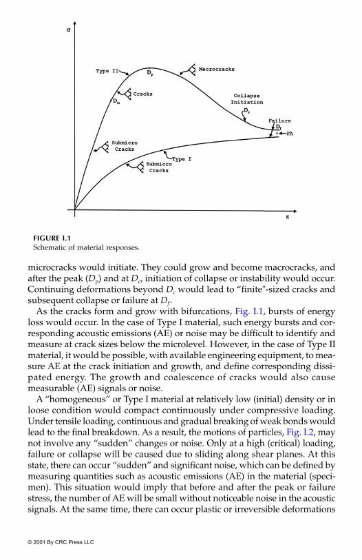
© 2001 By CRC Press LLC
Mechanics of Materials and Interfaces
microcracks would initiate. They could grow and become macrocracks, andafter the peak (Dp) and at Dc, initiation of collapse or instability would occur.Continuing deformations beyond Dc would lead to “finite"-sized cracks andsubsequent collapse or failure at Df.
As the cracks form and grow with bifurcations, Fig. I.1, bursts of energyloss would occur. In the case of Type I material, such energy bursts and cor-responding acoustic emissions (AE) or noise may be difficult to identify andmeasure at crack sizes below the microlevel. However, in the case of Type IImaterial, it would be possible, with available engineering equipment, to mea-sure AE at the crack initiation and growth, and define corresponding dissi-pated energy. The growth and coalescence of cracks would also causemeasurable (AE) signals or noise.
A “homogeneous” or Type I material at relatively low (initial) density or inloose condition would compact continuously under compressive loading.Under tensile loading, continuous and gradual breaking of weak bonds wouldlead to the final breakdown. As a result, the motions of particles, Fig. I.2, maynot involve any “sudden” changes or noise. Only at a high (critical) loading,failure or collapse will be caused due to sliding along shear planes. At thisstate, there can occur “sudden” and significant noise, which can be defined bymeasuring quantities such as acoustic emissions (AE) in the material (speci-men). This situation would imply that before and after the peak or failurestress, the number of AE will be small without noticeable noise in the acousticsignals. At the same time, there can occur plastic or irreversible deformations
FIGURE I.1Schematic of material responses.

© 2001 By CRC Press LLC
APPENDIX I
and dissipation of energy during the deformation process. One of the conse-quences of “continuous” irreversible deformations is the phenomenon of con-tinuous yielding, which can lead to the critical state (Chapter 7).
A deforming heterogeneous or brittle material of Type II, on the otherhand, develops microcracks or microfractures, which can nucleate and growinto clusters, and coalesce to form macrofractures. During this process, thematerial experiences irreversible deformations, and dissipation or release ofseismic (acoustic) energy. As a consequence, redistribution of stresses thatcannot be carried by the fractures (or failed parts) to the material parts in theintact state can take place. The process of microcracking can initiate some-where before or at the peak stress, Fig. I.3. The occurrence of the release ofseismic energy or seismic events can be measured as AE counts, and canexhibit noisy signals with different frequencies, Fig. I.3.
The NSA in the DSC implies bringing material particles or parts to a moreeffective relative configuration so as to optimally respond to external forces
FIGURE I.2Schematic of compactive and AE responses for relatively homogeneous (Type I) materials.

© 2001 By CRC Press LLC
Mechanics of Materials and Interfaces
or influences. The process of self-adjustment results in the evolution orgrowth of the material’s microstructure involving plastic yielding andmicrofracturing, or a combination of both, depending upon the nature of thecomposition and type of the material. The plastic yielding may not entail aprocess that causes sudden bursts of microcracks and energy, which can betermed as a relatively quiet phenomenon. On the other hand, microcracking(in a brittle material) may entail bursts of microcracks and energy, which canbe termed as a noisy or turbulent phenomenon.
The behavior of both the above types of materials, homogeneous, andheterogeneous, involving growth and evolution of yielding or microfrac-turing, can be explained on the basis of the NSA approach. As it will be dis-cussed later, the SOC can explain the response of brittle materials involving
FIGURE I.3Schematic of compactive-dilative, microfracturing and AE responses for relatively hetero-geneous brittle (Type II) materials.

© 2001 By CRC Press LLC
APPENDIX I
microfracturing and noisy signals (e.g., flicker or 1�f noise). CSC and SOCmainly explain the phenomenon at the (final) critical state when avalanchesand collapse (of the material’s microstructure) initiate, e.g., Dc, Fig. I.3. On theother hand, the DSC can explain the entire deformation behavior includingprepeak, postpeak, and critical or collapse. In other words, the DSC is consid-ered to be general, as it can include the states defined by the CSC and SOC asspecial cases.
Self-Organized Criticality
Bak and coworkers (1–4) have proposed the self-organized criticality (SOC)concept. It is based on the idea that a large complex system such as a granularmaterial containing many particles (components), under external influences,can evolve into a poised or critical state; its response is affected by past historyand events. At the critical state (increasing) minor disturbances can lead tocatastrophic events similar to those at the collapse or limiting critical state,called avalanches, of different sizes. Evolution of such a system to the criticalstate results as a consequence of the interactions between the constituents ofthe system. It was shown that a wide range of phenomena can be describedon the basis of the SOC, e.g., behavior of a sand pile, occurrence of earth-quakes, price variation of commodities, evolution and extinction of biologi-cal species, growth of cites, light from quasars and fluctuation of flow inrivers (4).
The SOC is often illustrated by using the behavior of a sand pile, Fig. I.4 (4).To start with, the sand pile is relatively flat and stable, and when sand grainsare added, they remain at the locations where they land. As sand grains are
FIGURE I.4Sandpile behavior (SOC).
© 2001 By CRC Press LLC
Mechanics of Materials and Interfaces
further added, the pile becomes steeper with an increase in the sliding ofgrains over the steep surfaces. At the critical (stage) slope, sliding can occurover almost all of the pile, when the behavior of the sand pile is out of balance,and catastrophic sliding events or avalanches can take place. Such eventscannot be understood in terms of the behavior of individual grains (compo-nents). In other words, in the behavior of avalanches, the coupling or itera-tion between the response of grains plays a vital role; thus, the behavior canbe understood or defined only on the basis of unified or holistic consider-ations. Bak and Tang (2) have noted that the behavior of a complex materialsystem may not be explained based on the response of individual particles,as in the micromechanics approach (5, 6).
In the SOC, the evolution of events (microfracturing, fluctuations in riverlevels, change in market prices, etc.) is characterized by long periods of sta-bility and short periods of rapid changes during which new events or formsappear. Such a phenomenon is often referred to as punctuated equilibrium (4),with periods of stasis (state of static balance of equilibrium or stable states)of different durations separated by bursts of activity, which gives rise to 1�for flicker noise and power law behavior. In the case of microfracturing inbrittle materials (Type II), the occurrence of microcracks and fracturesinvolving stable material states can be considered to exhibit punctuated equi-librium and stasis response.
It may be mentioned that the SOC (in the case of the sand pile) explains thephenomenon of collapse or avalanche formation. However, it dos not includethe mechanical response of the growing sand pile before it reaches the criticalstate. In other words, in the case of the behavior of engineering materials, theSOC defines the initiation of collapse state (Dc, Fig. I.1), but may not definethe entire pre- and postpeak response.
In engineering material systems, evolution of the critical states, in general,entails irreversible deformations, i.e., dissipation or release of energy. Theearth’s crust subjected to tectonic forces and motions of plates can lead to thecritical states or earthquakes. If we consider the relation between the flow ofsand (during sliding) with time, or the gradual developments of motions inthe earth’s crust leading to an earthquake, we would observe erratic signalsof different durations due to sudden crack formation and energy bursts. Suchsignals are called flicker noise or 1�f noise (pronounced as “one over ef”noise). The name 1�f noise indicates that the strength of a signal is inverselyproportional to its frequency (f).
The flicker or 1�f noise can be related to the systems that have evolved intothe critical state. Such systems exhibit a power law behavior given by
(I.1a)
where N is any quantity such as the number of earthquakes (or acoustic emis-sions) with given energy, for which Eq. (I.1a) can be expressed as
(I.1b)
N f( ) f ���
N s( ) s ���

© 2001 By CRC Press LLC
APPENDIX I
where s is the energy released by the earthquake and � is a parameter. Thewell-known empirical Gutenberg-Richter law (7, 8) for earthquakes followsEq. (I.1) and is given by
(I.2a)
where parameters a and b depend on the (regional) location, and N is thenumber of earthquakes of size (or magnitude) greater than m. The energy, E,released during the earthquake increases exponentially with its size, and isgiven by
(I.2b)
where c and d are parameters. Based on Eq. (I.2), the Gutenberg-Richter lawrepresents the power law, Eq. (I.1), that connects the released energy (E) withthe frequency distribution:
(I.3a)
where 1.25 � � � 1.5 (2). The relation between N and m can also be expressedas
(I.3b)
which represents a straight line on the log N vs. log m plot, Fig. I.5. In thisfigure, N represents the number of earthquakes (per year), and magnitude mis proportional to the released energy in the New Madrid seismic zone in thesoutheastern United States during the period 1974–83 (8).
FIGURE I.5Distribution of earthquake magnitudes in New Madrid zone (8). ©American GeophysicalUnion.
log10 N a bm��
log10 E c dm��
dNdE-------- m ��
�
log N � log m��

© 2001 By CRC Press LLC
Mechanics of Materials and Interfaces
In the critical state concept (CSC) (9), a deforming material with given initialpressure approaches the critical state at which it continues to deform in shearunder the constant shear stress with constant density or void ratio (Chapter 3).The initiation of the critical state can be considered to imply initiation of col-lapse of the material. In this sense, the basic idea in the SOC that defines thebehavior of a system that evolves to collapse can be considered to be similarto the CSC. This has been shown by Evesque (10) on the basis of the stabilityresponse of glass spheres in a rotating drum, by using Eqs. (3.2a) and (3.2b),Chapter 3.
The foregoing brief descriptions suggest that a natural system (like an engi-neering material) composed of interacting particles or clusters of particlesunder external influences (forces, temperature, chemicals, etc.) can evolveinto catastrophic states, affected by the past history, due to the self-organiza-tion of the internal microstructure of the system. As discussed in variouschapters in this book, a deforming material evolves from the RI state to theFA state. During this process, the material’s microstructure can experienceirreversible deformations and energy release for homogeneous (Type I) mate-rials, while it may experience both the energy release and microfracturing forbrittle materials (Type II). Both may exhibit a power law type behavior; how-ever, the occurrence of the 1�f noise may usually be observed and measurableonly in the case of microfracturing. In other words, it is believed that the SOCthat is based on the power law behavior, steady states and 1�f noise, at thistime may be defined mainly in the case of microfracturing response.
The DSC, with the NSA idea, can explain both the foregoing responses andcan allow the characterization of the entire (prepeak, postpeak, and critical orcatastrophic) behavior, Figs. (I.1)–(I.3). The overall behavior can experience anumber of threshold transitions in its microstructure such as the transitionfrom compactive to dilative volume, peak stress, and the critical condition, atDc (11–13), Fig. I.3.
Acoustic Emissions
One of the ways to ascertain if the deforming material exhibits noisy (1�ftype) behavior is to perform indirect (nondestructive) measurements such asacoustic emissions. Although a number of studies have considered themicrofracturing behavior, including measurements of AE, there are not manyresults available for the measurement of AE in homogeneous (Type I) mate-rials. Figure I.6 shows computer simulations of stress-strain, AE and dissi-pated energy responses of a relatively (or more) heterogeneous rockspecimen (with homogeneity index m � 1.5), and relatively (or more) homo-geneous rock specimen (m � 3) reported by Tang and Kaiser (14,15); detailsof the computer simulation are given later in Example I.3. It can be seen thatthe response of the heterogeneous rock involves relatively “noisy” AE distri-bution. On the other hand, the homogeneous rock does not involve signifi-cant AE in the prepeak and postpeak regions; the major AE occur near thepeak stress where failure due to sliding is indicated. Thus, the response of the

© 2001 By CRC Press LLC
APPENDIX I
relatively heterogeneous rock indicates dispersed microcracking with AEthat exhibit sudden bursts and noise, while that for the relatively homoge-neous rock shows sudden bursts only near the peak. However, both mayexhibit power law type behavior; this is shown in Fig. I.7 for the relativelyheterogeneous rock. Here, the number of acoustic events for given AE countwere taken from Fig. I.6; because the details of the laboratory data are notavailable, the values are essentially approximate. The rock exhibits powerlaw behavior given by
(I.4)
where the value of � � 166.15 and � � 1.012. Since sufficient data is not avail-able from Fig. I.6 for the homogeneous rock, it is not possible to obtain a sim-ilar plot.
In the following, we consider examples of the behavior of a number ofmaterials including correlations and comparisons between the DSC and SOC.
Example I.1: Simulated Microfracturing Phenomenon in Elastoplastic MaterialsZapperi et al. (16), performed numerical tests by considering the “fuse” modelconstituting a resistor network system on a tilted square lattice. The disorder(or heterogeneity) was introduced in the model by assigning a random failure
FIGURE I.6Numerical simulation of tests for rock specimens (14). (Reprinted with permission fromElsevier Science.)
N � AE( ) ���

© 2001 By CRC Press LLC
Mechanics of Materials and Interfaces
threshold, Ic, to each resistor, where Ic is the critical current analogous to stress.In the classic fuse model, failure is identified when the current flowing in aresistor exceeds the failure threshold, Ic ; then the bond is removed from the lat-tice, and the electrical conductivity (c) drops to zero. Thus, the (resistor) modeldevelops a macroscopic crack and eventually the lattice breaks. The simulatedtest (16) introduced permanent “damage” to the bond by decreasing its con-ductivity by a factor a � (1 � �), where � is the damage parameter, [Eq. (4.23),Chapter 4]. The analogy to linear elastic behavior can be used by expressingthe observed or actual stress, , as
(I.5a)
where is the elastic constitutive matrix. Thus, the reduction in the conduc-tivity, a, denotes the reduction in the initial stiffness, , which is equivalentto the conductivity during the application of current, I; the voltage, V, is anal-ogous to the strain. For the resistor model, Eq. (I.5a) can be written as
(I.5b)
It may be noted that Eq. (I.5) represents the classical damage model [Eq.(4.24), Chapter 4]. In the context of the DSC, the general form of Eq. (I.5) will
FIGURE I.7Number of AE events vs. AE event and determination of � and �.
a
˜
a 1 D�( )˜
i 1 D�( )C˜
i˜
i� �
C˜ C
˜
Ia 1 D�( )Ii 1 D�( )ci Vi�� �

© 2001 By CRC Press LLC
APPENDIX I
be given by
(I.6)
where and are relevant to the FA material parts. It is believed that Eq. (I.6)can lead to more realistic representation of the behavior of the resistor modelbecause it allows for the coupling between the undamaged and damaged parts(Chapter 4). Zapperi et al. (16) used the simplified Eq. (I.5). Such approximations(14–16) do not allow for the nonlinear response, which many materials exhibit.
In the resistor model test, an external voltage (strain) difference is appliedto the lattice with periodic boundary conditions in the other direction. Thecurrent in each bond or resistor node is computed by solving numericallythe Kirchoff equation using a multigrid relaxation algorithm with precision � . As the voltage is increased, the current (stress) reaches the thresh-old value in (number of) bonds. For such damaged bonds, the disorder ischanged according to the reduction in the conductivity. The process isrepeated under new currents until no unstable bonds are present. The“redistribution” of the disorder can cause an avalanche of additional bondsbreakage after the failure of a single bond. The network system was studiedin the limit of slow driving, implying that the time scale over which micro-fractures form and propagate is much faster than the time scale of the exter-nal driving (voltage). This condition is one of the characteristics of systemsthat exhibit SOC (4).
During the application of increasing voltage, initially there occurs propor-tional increase in the total current (stress); i.e., the system behavior is linearlyelastic, Fig. I.8(a). With further increase in the voltage and development ofdamage and broken bonds, the system deviates from linear elasticity,becomes macroscopically plastic, and approaches the steady state. In thisstate, an increase in the voltage (strain) is balanced by the damage such thatthe current (stress) remains approximately constant, and it is accompanied byhigh fluctuations (in the current), with avalanches of different sizes.
Zapperi et al. (16) studied the statistical properties of the bond breakage,fracture, or rupture events in time and the magnitude of fracturing, Fig. I.8(b).The avalanche or rupture event size probability distribution function, P(s),was found to be given by
(I.7)
where s is the number of damaged bonds for a given voltage increment,Fig. I.8(b), and � � 1.19 � 0.01. Figure I.8(c) shows the plot of P(s) vs. s fordifferent sizes of the model (L � 16, 32, 64). It can be seen that the responseof the system experiencing microfracture and rupture events displays thepower-law behavior. The distribution of energy bursts during the testingwas found to be related to the acoustic emissions recorded, and alsoexhibited the power-law behavior (16–18).
Ia 1 D�( )ciVi Dcc Vc� �
cc Vc
10 12�
P s( ) s ���
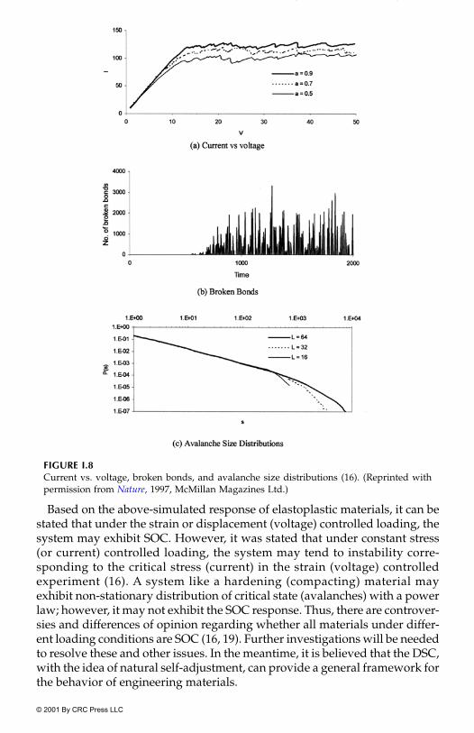
© 2001 By CRC Press LLC
Mechanics of Materials and Interfaces
Based on the above-simulated response of elastoplastic materials, it can bestated that under the strain or displacement (voltage) controlled loading, thesystem may exhibit SOC. However, it was stated that under constant stress(or current) controlled loading, the system may tend to instability corre-sponding to the critical stress (current) in the strain (voltage) controlledexperiment (16). A system like a hardening (compacting) material mayexhibit non-stationary distribution of critical state (avalanches) with a powerlaw; however, it may not exhibit the SOC response. Thus, there are controver-sies and differences of opinion regarding whether all materials under differ-ent loading conditions are SOC (16, 19). Further investigations will be neededto resolve these and other issues. In the meantime, it is believed that the DSC,with the idea of natural self-adjustment, can provide a general framework forthe behavior of engineering materials.
FIGURE I.8Current vs. voltage, broken bonds, and avalanche size distributions (16). (Reprinted withpermission from Nature, 1997, McMillan Magazines Ltd.)

© 2001 By CRC Press LLC
APPENDIX I
Example I.2: Microfracturing and Acoustic Emissions in Laboratory Tests for RockCox and Meredith (20) performed unconfined compression tests on cylindricalspecimens (25 mm dia. and 72 mm long), Fig. I.9(a), of Gosford sandstone fromNSW, Australia. The rock has porosity of 13% and contains mostly sub-angularto sub-rounded quartz and quartzite grains with diameters in the range of0.1–1.0 mm, with about 20% fine-grained clay and polycrystalline mica matrixmaterial. The specimens are tested under strain-controlled loading at a con-stant rate of axial shortening. Acoustic emissions are measured by using PZTAE sensors located in cavities within the end platens, Fig. I.9(a).
The stress-strain behavior of one of the specimens, shortened at the rate of0.495 �m�sec (approximate strain rate � 7 � �sec) is shown in Fig. I.9(b).The stress vs. time (which bears approximately linear relation to strain) andAE or hit rate vs. time are shown in Figs. I.10(a) and (b), respectively. It canbe seen from Figs. I.9(b) and I.10(a) that during the linear elastic phase of thestress-strain response, very few AE occurred because the active deformation
FIGURE I.9Rock specimen and stress-strain response: strain rate � 0.495 �m�sec (�7 � 10�6/sec) (20).(Reprinted with permission from Elsevier Science.)
10 6�

© 2001 By CRC Press LLC
Mechanics of Materials and Interfaces
mechanisms (pore-crack closure and elastic shortening) are continuous. In thezone beyond the linear elastic in which irreversible deformations occur, therate of AE increases because of discontinuities due to microfractures andcracks. The maximum rate occurs near the peak and stress drop region, andthen decreases in the post-drop region.
The AE rates at different times were computed (approximately) based on Fig.I.10(b). They were then ranked in descending order, Table I.1. Figure I.11 showsa plot of AE rate vs. rank on log-log scale. This plot is similar to that proposed inthe Zipf’s law (21). The (average) value of � (Fig. I.11) is found to be 1.558 with �� 316.65, indicating the power-law behavior as in the SOC.
FIGURE I.10Stress vs. time and hit (AE) rate vs. time for rock specimen, Figure I.9 (20). (Reprinted withpermission from Elsevier Science.)
FIGURE I.11AE rate vs. rank: Test on rock specimen.
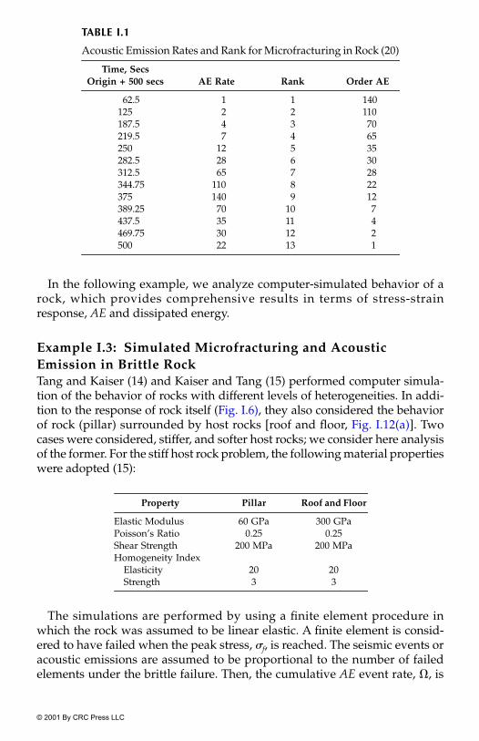
© 2001 By CRC Press LLC
APPENDIX I
In the following example, we analyze computer-simulated behavior of arock, which provides comprehensive results in terms of stress-strainresponse, AE and dissipated energy.
Example I.3: Simulated Microfracturing and Acoustic Emission in Brittle RockTang and Kaiser (14) and Kaiser and Tang (15) performed computer simula-tion of the behavior of rocks with different levels of heterogeneities. In addi-tion to the response of rock itself (Fig. I.6), they also considered the behaviorof rock (pillar) surrounded by host rocks [roof and floor, Fig. I.12(a)]. Twocases were considered, stiffer, and softer host rocks; we consider here analysisof the former. For the stiff host rock problem, the following material propertieswere adopted (15):
The simulations are performed by using a finite element procedure inwhich the rock was assumed to be linear elastic. A finite element is consid-ered to have failed when the peak stress, f, is reached. The seismic events oracoustic emissions are assumed to be proportional to the number of failedelements under the brittle failure. Then, the cumulative AE event rate, �, is
TABLE I.1
Acoustic Emission Rates and Rank for Microfracturing in Rock (20)
Time, Secs Origin + 500 secs AE Rate Rank Order AE
62.5 1 1 140125 2 2 110187.5 4 3 70219.5 7 4 65250 12 5 35282.5 28 6 30312.5 65 7 28344.75 110 8 22375 140 9 12389.25 70 10 7437.5 35 11 4469.75 30 12 2500 22 13 1
Property Pillar Roof and Floor
Elastic Modulus 60 GPa 300 GPaPoisson’s Ratio 0.25 0.25Shear Strength 200 MPa 200 MPaHomogeneity Index
Elasticity 20 20Strength 3 3

© 2001 By CRC Press LLC
Mechanics of Materials and Interfaces
FIGURE I.12Pillar-stiff host rock model and simulated stress-strain, AE, and energy responses.

© 2001 By CRC Press LLC
APPENDIX I
considered to be proportioned approximately to damage or disturbance (D)as
(I.8a)
where D is the damage given by
(I.8b)
vf is the volume of failed element, V is the total volume, ni is the number offailed elements, s is the number of calculation steps, and N is the total numberof elements in the (FE) mesh. The cumulative seismic energy (E), assumingbrittle failure at f, is given by (15)
(I.9)
where Cf is the elastic modulus, and Ef is the released energy for a givenelement. The magnitude, mf , of an individual microseismic event, and themagnitude, Mf, of the seismic event cluster are obtained from (15)
(I.10a)
and
(I.10b)
where i is the number of events in an event cluster and C is the constant.It may be noted that the above model is based on simple linear elastic char-
acterization in which the “damaged” elements have no strength, as in theclassical damage model. In actuality, the rock behavior is usually nonlinear,and the FA (or damaged) elements can possess certain strength and interactwith the RI elements as in the DSC. If such interactions were allowed, thecomputed simulations can be different.
Figure I.12(b)–(d) (22) show the stress, cumulative AE and E/Emax vs. strainfor the pillar in the stiff host rock model, Fig. I.12(a); details of plots showingAE counts at different loading steps and formation of shear planes leading tofailure are given in (15).
Figures I.12(b)–(d) show that the highest number of AE and magnitude ofenergy dissipation occur around the first stress drop, Fig. I.12(a), after thepeak stress. Then a number of stress drops occur in the descending part of thecurve, and each drop is associated with elevated AE and energy release. Forthe pillar-stiff host rock model, the energy stored in the host rock that can be
� D 1N---- ni
i�1
s
�� �
D�v f
V---------�
E �E fve
2---- �
f2
C f------�
m f log E f( ) C �
M f E fii�1
n
�
log C �
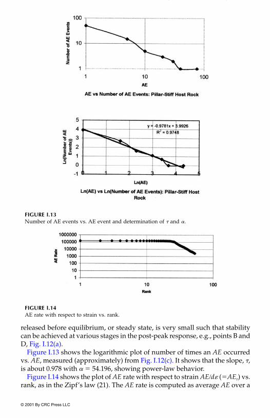
© 2001 By CRC Press LLC
Mechanics of Materials and Interfaces
released before equilibrium, or steady state, is very small such that stabilitycan be achieved at various stages in the post-peak response, e.g., points B andD, Fig. I.12(a).
Figure I.13 shows the logarithmic plot of number of times an AE occurredvs. AE, measured (approximately) from Fig. I.12(c). It shows that the slope, �,is about 0.978 with � � 54.196, showing power-law behavior.
Figure I.14 shows the plot of AE rate with respect to strain AE�d (�AEr) vs.rank, as in the Zipf’s law (21). The AE rate is computed as average AE over a
FIGURE I.13Number of AE events vs. AE event and determination of � and �.
FIGURE I.14AE rate with respect to strain vs. rank.

© 2001 By CRC Press LLC
APPENDIX I
given strain range divided by the corresponding strain increment. This issimilar to the analysis by Petri (18) in which the number of broken bondsbetween two consecutive stretches (strains) are considered. The relationbetween (AE)r and rank (R) is given by
(I.11)
The value of �, Fig. I.14, is found to be about 1.42 and � � 32 � .
Disturbance, AE, and Energy
The disturbance, D, can be expressed based on the stress-strain response,Fig. I.12(b), where the RI response is simulated as nonlinear elastic or elasto-plastic:
(I.12a)
in which ≈ 17.0 MPa. In terms of plastic strains, , disturbance is expressedas
(I.12b)
where Du � 1 is assumed. The plastic strains, , are computed as
(I.12c)
where t denotes the total strain, Fig. I.12(b), and is the elastic straincomputed by using elastic modulus, E ≈ 6.67 � MPa. Figure I.15 showscomputed, Eq. (I.12b), and measured, Eq. (I.12a), disturbance, with respect to. The values of A1 and Z1 were found by plotting ln[�ln(1 � D)] vs. ln();their values were found to be A � 48.584 and 1.522, respectively.
The variations of the norm of AEn (AE�515), Fig. I.12(c), and of E/Em, Fig. I.12(d),can also be expressed in terms of plastic strains as
(I.13a)
and
(I.13b)
AE( )r �R ���
105
D
i
a
�
i
c
�------------------�
c
D 1 e A1 Z1���
t
e
��
e
104
AEn 1 e A2Z2���
E Em� 1 e A3Z3���

© 2001 By CRC Press LLC
Mechanics of Materials and Interfaces
The values of A2 � 45.792 and Z2 � 1.192, and A3 � 168.629 and Z3 � 1.912 werefound corresponding to Eqs. (I.13a) and (I.13b), respectively. Figures I.16(a) and(b) show computed variations of AEn and E�Em vs. plastic strains, Eq. (I.13). Itcan be seen from Figs. (I.15) and (I.16) that the disturbance, AEn and E�Em,show similar relationships with respect to plastic strains. Also, they can becorrelated; Figs. I.17(a) and (b) show such relations between disturbance andAE and E�Em. In fact, the relations can be expressed as
(I.14a)
(I.14b)
The foregoing analyses show that there exist correlations between distur-bance, acoustic emissions and energy dissipation. Hence, the behavior of therock can be explained by using disturbance as the measure of microstruc-tural changes. This is further illustrated in Fig. I.18, where the disturbancerate (Dr) with respect to strains is plotted with rank; in Fig. (I.14), a similarplot for energy rate is presented. The behavior in Fig. I.18 exhibits the powerlaw with � � 1.027 and � � 1228.68.
In Fig. I.19(a)–(c) are plotted the variations of derivatives of disturbance,Eq. (I.12b), AEn, Eq. (I.13a), and E�Em, Eq. (I.13b), with plastic strains; theyshow behavior similar to the AE rate measured in the laboratory test on rock,Fig. I.10b. At the initiation of the collapse or residual condition, the plasticstrain is about 0.12% and occurs at the critical value, Dc ≈ 0.90, (AEn) ≈ 0.95,and (E�Em)c ≈ 0.97.
FIGURE I.15Measured and modeled disturbance vs. plastic strain.
DAE 1 eA4 AEn( ) Z4�
��
DE 1 eA5 E�Em( ) Z5�
��

© 2001 By CRC Press LLC
APPENDIX I
Example I.4: Instability and Liquefaction During EarthquakeWe now present analysis of the Port Island, Japan earthquake in 1995, duringwhich data for measured shear wave velocities, stress-strain behavior and dis-sipated energy were available (23). These results were used to identify liquefac-tion based on the DSC and energy approaches (12).
Figures I.20(a) and (b) show soil details and instruments, and typical mea-surements of shear wave velocities with time, respectively. Figures I.21(a)and (b) show dissipated energy vs. time and typical shear stress-straincurves, respectively. Figure I.22 shows disturbance (D) with time at variousdepths. Disturbance was computed on the basis of shear wave velocities [Eq.3.9, Chapter 3] in which the RI shear wave velocity, � 250 m�s, and the FAvelocity, � 25 m�s, were adopted; relates to average velocity in theupper saturated soil layer, Fig. I.20(b) before the earthquake, and repre-sents the fully adjusted or residual velocity after the earthquake shaking. It
FIGURE I.16Computed AE norm and E�Em vs. plastic strain.
Vi
Vc Vi
Vc

© 2001 By CRC Press LLC
Mechanics of Materials and Interfaces
was found that the soil experienced instability and liquefaction after about14.6 seconds during the earthquake when the shear wave velocity was about42 m�s and the critical disturbance, Dc ≈ 0.905, Fig. I.22.
The dissipated energy and disturbance rates, Er and Dr, were computedwith respect to time. Here, average values of energy or disturbance, Figs. I.21and I.22, over a given time range were divided by the corresponding timeincrement. Figures I.23(a) and (b) show Er and Dr versus Rank (R) on the log-arithmic scale. The values of the exponent, �, were found to be about 1.182and 1.1416, and � � 27.27 and 6.45 for Er and Dr, respectively, showing the
FIGURE I.17Relations between AE norm and E/Em, and disturbance.
FIGURE I.18Disturbance rate vs. rank.

© 2001 By CRC Press LLC
APPENDIX I
power-law behavior. However, the existence of 1�f noise cannot be verifiedfor this case. This is because the saturated soil under earthquake loadingexperiences continuous compaction, which causes increase in the pore waterpressure. When the pore water pressure approaches the critical value (criticaldisturbance, Dc), microstructural instability or liquefaction occurs (11–13).This compaction phenomenon essentially involves particle motions and maynot involve microfracturing that may usually be responsible for 1�f-typenoise.
FIGURE I.19Plots of derivatives of D, AE norm, and E�Em vs. plastic strain.

© 2001 By CRC Press LLC
Mechanics of Materials and Interfaces
FIGURE I.19(continued)
FIGURE I.20Soils, instruments, and measured shear wave velocities, Port Island, Kobe site (23).
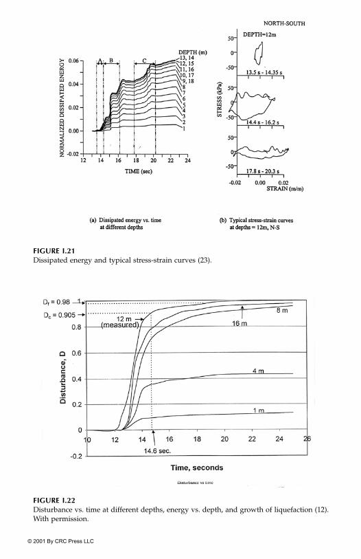
© 2001 By CRC Press LLC
APPENDIX I
FIGURE I.21Dissipated energy and typical stress-strain curves (23).
FIGURE I.22Disturbance vs. time at different depths, energy vs. depth, and growth of liquefaction (12).With permission.

© 2001 By CRC Press LLC
Mechanics of Materials and Interfaces
Example I.5: Cyclic Behavior of Saturated SandsWe consider laboratory behavior of two saturated sands, Reid Bedford (24)and Ottawa (11–13, 25), tested by using torsional shear and multiaxialdevices, respectively.
Figure I.24 shows the shear stress vs. strain and time (10 points�sec), andpore water pressure vs. time responses for the sand specimen with relativedensity Dr � 60%, initial mean pressure po � 124.10 kPa tested under cyclicstrain-controlled condition (frequency = 0.10 Hz) with amplitude of shearstrain � 47%. Figure I.25 shows plots of disturbance (D) and accumulatedenergy per unit volume with number of cycles (N). The values of D werefound based on the stress-strain response, Fig. I.24(a). Figure I.26(a) showsenergy rate Er vs. Rank; Er was computed as the ratio of average energy overa range of pore water pressure to the pore water pressure increment. FigureI.26(b) shows disturbance rate vs. rank. The value of � � 0.341 and 0.327, and� � 2155.98 and 1.17, respectively, are indicated.
Cyclic stress-controlled (frequency � 0.10 HZ) tests were performed oncubical (10 � 10 � 10 cm) specimens of saturated Ottawa sand with Dr � 60%and initial effective confining pressures � 69, 138, and 207 kPa. The mea-surements were obtained in terms of stress, strain, and pore water pressureresponses (25). The results for pore water pressure (Ue) vs. time for the threeconfining pressures are shown in Fig. I.27. The effective stress was com-puted as the difference between the total stress, , and pore water pressure,Ue ; Fig. I.28 shows plots of vs. N. The disturbance was computed by
FIGURE I.23Energy rate and disturbance with respect to time vs. rank: Port Island earthquake.
�o
�
�

© 2001 By CRC Press LLC
APPENDIX I
assuming the RI behavior to be elastoplastic with the HISS �0-plasticitymodel (Chapter 7), given by
(I.13)
where is the asymptotic effective stress, which can be adopted to be zero.Figure I.29 shows the plot of the disturbance rate, Dr, with respect to pore
water pressure vs. the rank; the values of � � 1.886 and � � 1.986.
FIGURE I.24Test results for Reid Bedford sand (24) (with permission).
D �i( )
�a( )
�
�i( )
�c( )
�-----------------------------�
�c( )

© 2001 By CRC Press LLC
Mechanics of Materials and Interfaces
As indicated earlier, the saturated sand under shear loading (strain andstress controlled) experiences compaction and reaches unstable or collapse orliquefaction condition when the pore water pressure becomes approximatelyequal to the initial effective pressure. During the process, the material’smicrostructure can experience continuing compaction without (measurable)1�f-type noise. Hence, the behavior may not be considered to exhibit SOC-type response. However, the microstructural evolution can be explained interms of self-adjustment in the DSC.
Summary
The foregoing review and analysis indicate that the DSC, with the micro-structural self-adjustment approach, can explain mechanical behavior of awide range of material systems. The disturbance, D, provides for evolutionof both the continuous yielding and microfracturing responses, and can becorrelated to dissipated energy and nondestructive measures such as acous-tic emissions. The DSC provides characterization of the entire material
FIGURE I.25Disturbance and accumulated energy vs. time (N): Reid Bedford sand.

© 2001 By CRC Press LLC
APPENDIX I
response including prepeak, peak, postpeak, and collapse or failure. On theother hand, the CSC and SOC provide definition of collapse or critical state;in this context, the DSC is considered to be general, because it includes thecollapse state defined by the CSC and SOC as a special case.
References
1. Bak, P., Tang, C., and Weisenfeld, K., “Self-Organized Criticality: An Explana-tion of 1�f Noise,” Physical Review Letters, 59, 4, 1987, 381–384.
2. Bak, P. and Tang, C., “Earthquakes as a Self-Organized Critical Phenomenon,”J. of Geophysical Research, 94, 311, 1989, 15635–15637.
3. Bak, P. and Chen, K., “Self-Organized Criticality,” Scientific American, January1991, 26–33.
4. Bak, P., How Nature Works: The Science of Self-Organized Criticality, Copernicus:Springer-Verlag, New York, 1996.
5. Nemat-Nasser, S. and Hori, M., Micromechanics: Overall Properties of Heteroge-neous Materials, North-Holland, Amsterdam, 1993.
FIGURE I.26Energy and disturbance rate with respect to cycles vs. rank: Reid Bedford sand.

© 2001 By CRC Press LLC
Mechanics of Materials and Interfaces
6. Okai, Y. and Horii, H., “A Micromechanics-Based Continuum Theory forMicrocracking Localization of Rocks under Compression,” Chapter 2 in Con-tinuum Models for Materials with Microstructure, H. B. Mühlhaus (Editor), JohnWiley, Chichester, UK, 1995, 27–68.
7. Gutenberg, B. and Richter, C. F., Seismicity of the Earth, Princeton UniversityPress, Princeton, NJ, 1949.
8. Johnston, A. C. and Nova, S., “Recurrence Rates and Probability Estimated forthe New Madrid Seismic Zone,” J. of Geophysical Research, 90, 1985, 6737.
9. Roscoe, K. H., Schofield, A. N., and Wroth, C. P., “On Yielding of Soils,”Geotechnique, 8, 1958, 22–53.
FIGURE I.27Multiaxial test results for excess pore water pressure for Ottawa sand (11–13, 25).

© 2001 By CRC Press LLC
APPENDIX I
10. Evesque, P., “Analysis of the Statistics of Sandpile Avalanches Using Soil-Mechanics Results and Concepts,” Physical Review A, The American PhysicalSociety, 43, 6, 1991, 2720–2740.
11. Desai, C. S., Park, I. J., and Shao, C., “Fundamental Yet Simplified Model forLiquefaction Instability,” Int. J. Num. and Analyt. Meth. Geomech., 22, 1998,721–748.
12. Desai, C. S., “Evaluation of Liquefaction Using Disturbed State and EnergyApproaches,” J. of Geotech. & Geoenv. Eng., ASCE, 126, 7, 2000, 618–631.
FIGURE I.28Effective stress vs. number of cycles for Ottawa sand (13) (with permission).

© 2001 By CRC Press LLC
Mechanics of Materials and Interfaces
13. Park, I. J. and Desai, C. S., “Cyclic Behavior and Liquefaction of Sand UsingDisturbed State Concept,” J. of Geotech. and Geoenv. Eng., ASCE, 126, 9, 2000.
14. Tang, C. A. and Kaiser, P. K., “Numerical Simulation of Cumulative Damageand Seismic Energy Release During Brittle Rock Failure—Part I: Fundamen-tals,” Int. J. Rock Mech. Min. Sc., 35, 2, 1998, 113–121.
15. Kaiser, P. K. and Tang, C. A., “Numerical Simulation of Damage Accumulationand Seismic Energy Release During Brittle Rock Failure—Part II: Rib PillarCollapse,” Int. J. Rock Mech. Min. Sc., 35, 2, 1998, 123–134.
16. Zapperi, G., Vespignani, A., and Starkey, E. H., “Plasticity and AvalancheBehaviour in Microfracturing Phenomena,” Letter to Nature, Nature, MacmillanMagazines Ltd., 388, 1997, 658–660.
17. Petri, A., Paparo, G., Vespignani, A., Alippi, A., and Costantini, M., “Experi-mental Evidence of Critical Dynamics in Microfracturing Processes,” PhysicsReview Letters, 73, 1994, 3423–3426.
18. Petri, A., “Acoustic Emission and Microcrack Correlation,” Philosophical MagazineB, 77, 2, 1998, 491–498.
19. Sornette, D., “Power Laws without Parameter Tuning: An Alternative toSelf-Organized Criticality,” Physics Review Letters, 72, 1994, 2306.
20. Cox, S. J. D. and Meredith, P. G., “Microcrack Formation and Material Softeningin Rock Measured by Monitoring Acoustic Emissions,” Int. J. Rock Mech. Min.Sc., 30, 1, 1993, 11–24.
21. Zipf, G. K., Human Behavior and the Principle of Least Effort, Addison-Wesley,Cambridge, MA, 1949.
22. Desai, C. S. and Nickerson, M., “Analysis and Comparisons of DSC and SOC,”under preparation, 2000.
23. Davis, R. O. and Berrill, J. B., “Energy Dissipation and Liquefaction atPort Island, Kobe,” Bulletin of New Zealand Nat. Soc. of Earthquake Eng., 31,1998, 31–50.
24. Figueroa, J. L., Saada, A. S., Laing, L., and Dahisaria, M. N., “Evaluation of SoilLiquefaction by Energy Principles,” J. Geotech. Eng., ASCE, 120, 9, 1994,1554–1569.
25. Gyi, M. M. and Desai, C. S., “Multiaxial Cyclic Testing of Saturated OttawaSand,” Report, Dept. of Civil Eng. and Eng. Mech., University of Arizona, Tucson,AZ, 1996.
FIGURE I.29Disturbance rate with respect to pressure vs. rank: Ottawa sand.

© 2001 By CRC Press LLC
APPENDIX II. DSC Parameters: Optimization and Sensitivity
In previous chapters, we discussed procedures for the determination of parame-ters in the DSC and its hierarchical versions, namely, elasticity, plasticity and elas-toviscoplasticity, and disturbance by using essentially manual and conventionalleast-square procedures. In this appendix, we present details of the conventionalleast square, and general optimization procedures for the evaluation of parameters.We also consider the sensitivity of computed results to changes in the parameters.
The observed behavior of many materials may exhibit considerable scattereven for the test specimens reconstituted under the same initial conditions.Also, factors such as initial density, confining pressure, temperature, strainrates, and stress path need to be considered because the objective is to evolvethe constitutive model that is valid for all such significant factors. Indeed, theaveraging or optimization procedure may lead to parameters that may predictbehavior under one factor better than that for the other. By assigning appro-priate weight in the averaging or optimization procedure for a factor(s) thatis more significant for a given problem, it is possible to obtain parameters thatwill lead to improved predictions for the given material.
Least Square Fit Procedure
We need to determine the parameters on the basis of laboratory test data suchas stress-strain, volumetric and pore water pressure. In general, the mea-sured quantities such as stress and strain can be denoted by symbols y and x,respectively. Then the function to fit the given set of data points (xi, yi, i � 1,2, …, n), Fig. II.1, can be expressed as (1)
(II.1)
where ai (i � 1, 2, . . . , m) are the constants to be determined from the least-square criterion described below, and x and y denote the experimental data.Hence,
(II.2)
y a1 f 1 x( ) a1 f 2 x( ) … am f m x( )� � ��
yi ak f k xi( )k�1
m
��

© 2001 By CRC Press LLC
When the values of experimental data are substituted in Eq. (II.2), it will notbe satisfied; i.e., there will be residuals (Ri). Hence,
(II.3a)
The best fit with the experimental data is obtained by making the residualsas small as possible, which is achieved by finding the values of ai such thatthe sum of the squares of the residuals is a minimum, i.e.,
(II.3b)
which can be written in matrix rotation as
(II.4a)
where � [R1 R2 … Rn], and
(II.4b)
FIGURE II.1Function and data points.
ak f k x1( ) y1�k�1
m
� R1�
ak f k x2( ) y2�k�1
m
� R2�
�
ak f k xn( ) yn�k�1
m
� R3�
��ak------- Ri( )2
i� 0�
R˜
F˜
O˜
�
R˜
F˜
f 1 x1( ) f 2 x1( ) … f m x1( )f 1 x2( ) f 2 x2( ) … f m x2( )
�f 1 xn( ) f 2 xn( ) … f m xn( )
�

© 2001 By CRC Press LLC
By using Eqs. (II.3) and (II.4), we can obtain
(II.5)
where � [a1 a2 … am] and � [y1 y2 … yn]. Solution of the algebraic equa-tions (II.5) leads to values of ai that provide the best fit to the observed data,Fig. II.1.
We can assign different weights (wi) to different data points. In that case,the minimizing residual quantity is given by
(II.6a)
Then, Eq. (II.5) is modified as
(II.6b)
where is the diagonal matrix with w1, w2 ,… as diagonal elements.As an example, let us consider the evaluation of parameters a1 and �1 in the
hardening function, �, Eq. (7.11a), Chapter 7, which can be written as
(II.7)
With a number of data points, n (�i, �i), this equation can be written inmatrix notation as
(II.8)
which can be solved for a1 and �1 by using the least square procedure. Detailsof the procedures for finding parameters for the HISS and other plasticity anddisturbance models are given elsewhere (2–4).
Optimization Procedure
In the least square procedure, which is termed as conventional, we obtain theparameters for a given test data, and then average them over a number oftests, say, under different loading conditions and stress paths. It can alsoallow evaluation of weighted average values by using data points from a
F˜
TF˜
a˜
FTy˜
�
a˜
T y˜
T
w1R12 w2R2
2 … wnRn2
� � � minimum�
F˜
Tw˜
F˜
a˜
F˜
Tw˜
y˜
�
w˜
ln� �1ln� lna1���
1 ln�1
1 ln�2
�1 ln�n
lna1
�1�
ln�1
ln�2
�ln�n
�

© 2001 By CRC Press LLC
number of tests, in which each test (stress path) is assigned an appropriateweight.
However, the quality of the parameters is also affected by the constraintsarising from physical requirements. Hence, the quality of parameters can beimproved by including the effects of various factors such as stress paths anddensity, and the constraining conditions in an optimization procedure. Suchan optimization procedure developed for finding the parameters for the DSCmodel is described below (4).
Objective Function
In the optimization procedure, an objective function is defined (5). Here, theobjective function, r, which consists of weighted basic objective functions (ri)for different stress paths, is expressed as
(II.9)
where wi (� wi � 1) denotes the weights corresponding to the objective func-tions, ri.
For a given experimental response for a stress path, denotes the totalerror given by
(II.10)
where denotes predictions by the (DSC) model, f denotes the test (stress-strain) data, x1 and x2 are the end points of the sampling data, Fig. II.2, and is the vector of material parameters (see later). The ideal situation is that ,Eq. (II.10), vanishes. However, usually, the optimization procedure isdesigned such that is minimized, i.e., → 0.
The weights, wi, in Eq. (II.9) are adopted on the basis of experience andengineering judgment. For example, for the stability analysis of a slope ordam, the extension behavior, Fig. 7.13 (Chapter 7), is more significant, andhence, a greater weight is assigned to the extension test data. For the footingload on a half space, the compressive behavior is predominant; hence, its datacan be assigned a higher weight. Sometimes, as a simplification, data from allavailable stress path tests may be assigned equal weights such that � wi � 1.
Constraints
In an optimization procedure, the analysis is carried out under constraintsthat influence the objective function. In the case of the DSC model, the follow-ing constraints are introduced (see Chapters 2–12) for various parameters.Here in the DSC model, the RI response is characterized by using the HISS-0
r wiri��
r x˜
( )
r x˜
( ) 1x1 x2�------------------
f x˜
( )f
----------- 1�
2
xdx1
x2
��
f x˜
( )x˜r x
˜( )
r x˜
( ) r x˜
( )

© 2001 By CRC Press LLC
elastoplastic model.
Elastic
(II.11a)
Plasticity (HISS-0 Model)
As the hardening function � 0, Eq. (7.11a), the constraining condition forthe ultimate parameter, �, is given by
(II.11b)
The constraining condition for the parameter, �, for the shape of the yieldsurface is given by (Chapter 7).
(II.11c)
For the transition or phase change parameters, n, the condition is
(II.11d)
The optimization problem is to evaluate given by
(II.12)
such that is minimized. Here, the elements of are the parameters inthe DSC model that include elastic, elastoplastic (HISS-0), critical state (forFA behavior) and disturbance; Du � 1.0 is assumed.
FIGURE II.2Schematic of residual.
E 0, 0.5; G 0, K 0��� ��
�J2D
J12 1 �Sr�( ) 0.5�
-------------------------------------
0 � 0.756��
n 2.0�
x˜
x˜
E, , n, �, �, a1, �1, m, �, eoc , A, Z[ ]T
�
r x˜
( ) x˜

© 2001 By CRC Press LLC
Numerical Method for Optimization
A number of strategies are available for the optimization procedure. Theyinclude Newton’s method, quasi-Newton method with constrained orunconstrained minimization (5). Here, we present and use the quasi-Newtonmethod with unconstrained approach, which leads to a simplified procedure.
In the Newton’s method, the function, , Eq. (II.10), is obtained by usingtruncated Taylor series expansion at about point , Fig. II.3, as
(II.13)
where denotes the vector of DSC parameters, Eq. (II.12), and , is the vector of first partial derivatives or gradient vector given by
(II.14)
FIGURE II.3Schematic Taylor series expansion of a function. ©John Wiley & Sons Ltd. Reproduced withpermission.
f x˜
( )x˜ k
f x˜ k
˜�( ) qk
˜( )� f
˜k
g˜
k
T
12---
˜TG
˜ k˜���
x˜
˜
x˜ k�1 x
˜ k�� g x˜
( )
g˜
x˜
( ) �f x˜
( )�

© 2001 By CRC Press LLC
and G is the matrix of second partial derivatives or Hessian matrix given by
(II.15)
and qk is the resulting quadratic function.The iterative procedure involves evaluation of the parameters, which is
equal to where the correction minimizes . In the Newton’smethod, we need , , and at different points (k) so as to evaluate .The method gives well-defined solution if is positive definite. A disad-vantage of the Newton’s method is that we need to compute the Hessianmatrix, , which can be time-consuming. Hence, the simplified quasi-Newtonmethod given below is used here.
Quasi-Newton Method
Like the Newton’s method, the quasi-Newton method involves the line searchprocedure (5). However, the matrix, , is approximated by using the symmetricpositive definite matrix, , which is corrected during the iterative procedure.The following equations constitute the quasi-Newton method:
(II.16a)
(II.16b)
in which the matrix, , is updated during the iterations as , ,…,denotes the line search direction, and is the scalar line search step length,described below.
The initial matrix, , can be adopted as any positive definite matrix,which can be chosen as , where is the identity matrix:
(II.17)
The BFGS algorithm (6–9), named after the first letter of the last names ofthe four authors, is often used to evaluate iterated values of as
(II.18)
where .
x˜
( )
G˜
x˜
( ) �2 f x
˜( )�
x˜ k
˜ k� ˜ k q
˜k
˜ k( )
f˜ k
g˜
kG˜ k q
˜k
˜ k( )
G˜ k
G˜
G˜ k
H˜ k
s˜k H
˜ kg˜
k��
x˜ k�1 x
˜ k �ks˜k��
H˜ k H
˜ k�1 H˜ k�2 s
˜k
�
H˜ 1
H˜ 1 I
˜� I
˜
I˜
1 0 0 … 00 1 0 … 0� 0 0 0 … 1
�
H˜
H˜ k�1 Hk 1
�˜
TH˜ k�
˜˜
T�˜
----------------�
˜˜
T
˜
T�˜
---------��
˜�˜
TH˜ k H
˜ k�˜
˜
T�
˜
T�˜
-----------------------------------------
�
�˜
k g˜
k�1g˜
k��

© 2001 By CRC Press LLC
Line Search Strategy
A number of line search strategies have been proposed (5). One such strategyis depicted in Fig. II.4, and is found to be efficient and stable. The followingdescent and stability conditions are embedded in this strategy for the compu-tation of in Eq. (II.16b) (5):
(II.19a)
(II.19b)
where � is a scalar in the range of 0.0 to 0.5, and � is a scalar in the range of �to 1.0. The following equations are used for the evaluation of
(II.19a)
(II.19b)
where the prime denotes derivative.
FIGURE II.4Descent and stable conditions (5). ©John Wiley & Sons Ltd. Reproduced with permission.
�
f k f k�1 �g˜
T˜ k��
g˜
k�1
T s˜k � g
˜ks˜k
�
� �� 0.5 � �1�
1f 1 f�
� �1�( ) f 1�-------------------------------�
------------------------------------------�
� ��� �1�( ) f�f�1 f��( )
---------------------------�
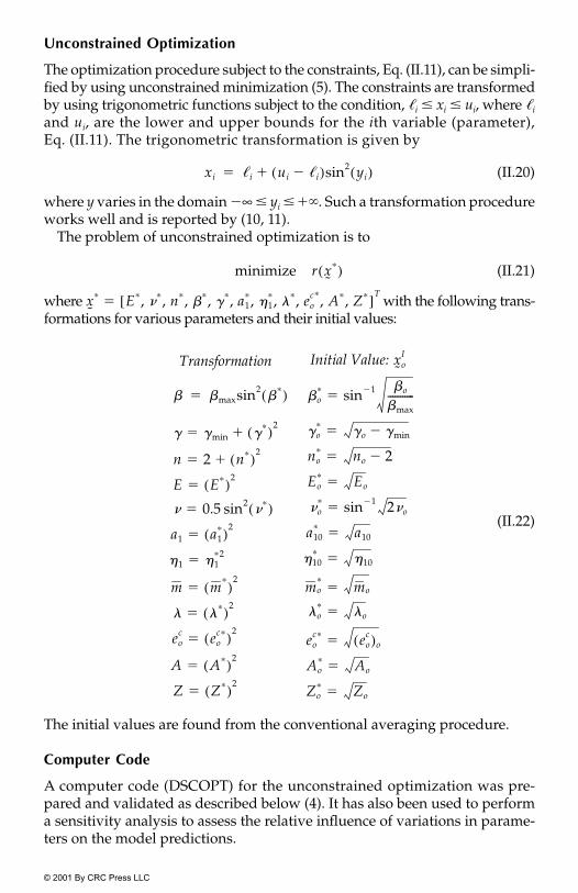
© 2001 By CRC Press LLC
Unconstrained Optimization
The optimization procedure subject to the constraints, Eq. (II.11), can be simpli-fied by using unconstrained minimization (5). The constraints are transformedby using trigonometric functions subject to the condition, �i � xi � ui, where �i
and ui, are the lower and upper bounds for the ith variable (parameter),Eq. (II.11). The trigonometric transformation is given by
(II.20)
where y varies in the domain �∞ � yi � . Such a transformation procedureworks well and is reported by (10, 11).
The problem of unconstrained optimization is to
(II.21)
where with the following trans-formations for various parameters and their initial values:
(II.22)
The initial values are found from the conventional averaging procedure.
Computer Code
A computer code (DSCOPT) for the unconstrained optimization was pre-pared and validated as described below (4). It has also been used to performa sensitivity analysis to assess the relative influence of variations in parame-ters on the model predictions.
xi �i ui �i�( )sin2 yi( )��
��
minimize r x˜
�( )
x˜
� � E�,
�, n�, ��, �
�, a1�, �1
�, ��, eo
c�, A�, Z�[ ]T
Transformation
� �maxsin2�
�( )�
� �min ��( )2
��
n 2 n�( )2��
E E�( )2�
0.5 sin2
�( )�
a1 a1�( )2
�
�1 �1�2
�
m m�( )
2�
� ��( )2
�
eoc eo
c�( )2�
A A�( )2�
Z Z�( )2�
Initial Value: x˜ o
I
�o� sin 1� �o
�max-----------�
�o�
�o �min��
no� no 2��
Eo� Eo�
o� sin 1� 2 o�
a10� a10�
�10�
�10�
mo�
mo�
�o�
�o�
eoc� eo
c( )o�
Ao� Ao�
Zo� Zo�

© 2001 By CRC Press LLC
Validations
The laboratory behavior of the Leighton Buzzard (LB) sand under differentstress paths, Fig. 7.13, Chapter 7, is used as the basis of the validation.Table II.1 shows details of the multiaxial tests on cubical specimens (10 �10 � 10 cm) of sand under different stress paths, confining pressure, (�3), andrelative density, Dr (12).
For the optimization analysis, the material parameters were found bydividing the test data in various groups. Groups 1–5, Table II.2(a), refer to thetests for Dr � 95%, while Table II.2(b) refers to the tests for Dr � 10%. In eachgroup, only selected stress path tests were used for finding the parameters.For example, in Group 1 three tests under HC, CTC (89.6 kPa), and CTC(275.6 kPa), were used, and so on. Equal weights, Eq. (II.9), were used foreach test in a given group.
The parameters were found by using the conventional (least square) aver-aging and the constrained optimization procedures. Then the stress-strain-volumetric responses of tests under different stress paths were predicted byusing the optimized parameters and those from the conventional procedures,
TABLE II.1
Laboratory Tests of Leighton Buzzard Sand (12)
Density (Dr) ConfiningPressure, kPaStress Path 95% 65% 10%
CTC(cylindrical)
� � � 89.6� � � 275.6� � � 826.8
RTE(cylindrical)
� � 89.6275.6
� 826.8HC(cylindrical)
� �
RTC(cubical)
� 89.6275.6826.8
TC (cubical)89.6
� 275.6826.8
TE (cubical)89.6
� 275.6826.8
� denotes the test performed.The void ratio: emax � 0.81, emin � 0.53.
Accordingly,Dr � 95% ⇒ e0 � 0.544Dr � 65% ⇒ e0 � 0.628Dr � 10% ⇒ e0 � 0.782

© 2001 By CRC Press LLC
and were compared with the observed behavior. Typical results for onlyselected groups are given below.
Tables II.3–II.5 show parameters for Groups 1 and 5 for Dr � 95% andGroup 6 for Dr � 10%, respectively. The percentage changes are with respectto the parameters from the conventional procedure.
TABLE II.2(a)
Groups for Dr � 95%
Data Set UsedStress Path Confining Stress (kPa) 1 2 3 4 5 Group
HC N�A � � � � �
CTC 89.6 � � � � �
CTC 275.6 �
CTC 826.8 �
RTE 89.6 �
TC 275.6 �
TE 89.6 �
TABLE II.2(b)
Group for Dr � 10%
Stress PathConfining Stress
(kPa)Data Set Used
6 Group
HC N�A �
CTC 89.6 �
CTC 275.6 �
CTC 826.8 �
TABLE II.3
Parameter Values Determined from Data Group 1
Parameter Conventional Optimized Change (%)
E 101450 kPa 104507 kPa �3.01 0.41 0.32584 �20.53n 2.537465 2.40913 �5.06� 0.7 0.60156 �14.06� 0.08102 0.0894954 �10.46a1 0.00296 3.00302E-4 �89.85�1 0.2849 0.298106 �4.64
0.00929 9.31397E-3 �0.26e0 0.544 0.544 0
0.683211 0.752341 �10.12� 0.0317 0.2940957 �827.75A 0.4579 0.84379 �84.27Z 0.3201 0.499684 �56.10
m
e0c

© 2001 By CRC Press LLC
Typical comparisons between predicted and observed stress-strain andvolumetric responses for different groups are shown in various figures asfollows:
It can be seen from Figs. II.5–II.7 that the predictions by using the opti-mized parameters yield much closer correlations with the observedresponses compared to those from the conventional procedures.
TABLE II.4
Parameter Values Determined from Data Group 5
Parameter Conventional Optimized Change (%)
E 40567.9 kPa 44194.6 kPa �8.94 0.4 0.35904 �10.24n 3 2.89034 �3.66� 0.75 0.75213 �0.28� 0.0827565 0.07904 �4.49a1 0.00128265 0.001282 �0.05�1 0.307546 0.31001 �0.80
0.102821 0.110981 �7.94e0 0.544 0.544 0
0.783012 0.679201 �13.26� 0.182442 0.2956 +62.02A 0.965391 0.889101 �7.90Z 0.29839 0.27092 �9.21
TABLE II.5
Parameter Determined from Data Group 6
Parameter Conventional Optimized Change (%)
E 35456.1 kPa 42830.5 kPa �20.80 0.4 0.379 �5.25n 2.6 2.758 �6.08� 0.7 0.751456 �7.35� 0.049215225 0.05315372 �8.00a1 0.00122739 0.00102946 �16.13�1 0.304157 0.3375602 10.98
0.268212 0.2459786 �8.29e0 0.544 0.544 0
0.0327233 0.02002876 �38.79� 0.0194252 0.0234572 �20.76A 1.53464 1.300956 �15.23Z 0.0800357 0.0689714 �13.82
Figure Group Stress Path �3 Density
Fig. II.5 1 CTC 89.6 kPa 95%Fig. II.6 5 TE 89.6 95%Fig. II.7 6 CTC 826.8 10%
m
e0c
m
e0c

© 2001 By CRC Press LLC
Effect of Weight
In the previous analysis, equal weights were assigned to each stress path. Inorder to assess the effect of weights on the predicted behavior, three special anal-yses were performed by using the CTC (�3 � 89.6 kPa) and RTE (�3 � 89.6 kPa)stress paths in Group 3, Table II.2(a):
(i) wCTC � wRTE � 0.5(ii) wCTC � 0.65, wRTE � 0.35
(iii) wCTC � 0.35; wRTE � 0.65
FIGURE II.5Comparisons between predictions and CTC test: Dr � 95%, �o � 89.6 kPa (4).

© 2001 By CRC Press LLC
Only results for the first two sets are presented here. Table II.6 showsparameters corresponding to the use of the sets of weights. The percentageerror is with respect to the equal weights.
Figure II.8 shows comparisons between predictions using equal weights (�0.5) and wCTC � 0.65 and wRTE � 0.35 for CTC test (�3 � 89.6 kPa, Dr � 95%).
It can be seen that the predictions for higher weight (� 0.65) for the CTC testyield improved predictions compared to those from the equal weight (� 0.50).
Thus, the predictive quality of the model can be improved by assigning higherweights to the stress paths that are important in a given practical problem.
FIGURE II.6Comparisons between predictions and TE test: Dr � 95%, �o � 89.6 kPa (4).

© 2001 By CRC Press LLC
Sensitivity of Parameters
A special study was performed to establish the sensitivity of the DSC predic-tions to the change in parameters and relative importance of the parameters.
Table II.7 shows the set of parameters adopted for this analysis. Predic-tions for stress-strain responses for CTC (�3 � 826.8 kPa, Dr � 10%) and RTE
FIGURE II.7Comparisons between predictions and CTC test: Dr � 10%, �o � 826.8 kPa (4).

© 2001 By CRC Press LLC
(�3 � 826.8 kPa, Dr � 10%) tests were obtained for three values of each param-eter; the value in Table II.7, and two other values as �20% and �20%. Allother parameters were kept constant, while a given parameter was thuschanged.
Figure II.9 shows averages of cumulative relative differences for the two(CTC and RTE) tests, which was found as
(II.23)
where q (� �1 � �3) denotes the observed stress, and denotes the computedvalue.
TABLE II.6
Effect of Weight on Parameter Values of Test Group 3 (wCTC � 0.65; wRTE � 0.35)
Parameter wCTC � wRTE � 0.5 wCTC � 0.65; wRTE � 0.35 Change (%)
E 354176.9 kPa 37334.2 kPa �6.13 0.3736 0.3549 �5.01n 2.48745 2.56391 �3.07� 0.755 0.6013 �20.36� 0.424063 0.498171 �17.48a1 0.0690234 0.0649979 �5.83�1 0.06012 0.05537 �7.90
0.199052 0.190444 �4.32e0 0.544 0.544 0
0.400987 0.431145 �7.52� 0.209711 0.347845 �65.87A 3.07893 2.84561 �7.58Z 0.199761 0.198043 �0.86
TABLE II.7
Parameters for Sensitivity Analysis
No. Parameter Value
1 E 143452 0.353 n 2.64 � 0.65 � 0.05025716 a1 0.0003862327 �1 0.71128 0.07900399 0.0883205
10 � 0.04958311 A 1.0153512 Z 0.4284032
m
e0c
me0
c
Cumulative Relative Differenceq q�
q-------------
��
q

© 2001 By CRC Press LLC
Table II.8 shows the order of the parameter sensitivity to computed results.It can be seen that the changes in the phase change (n), ultimate slope of yieldsurface (�), hardening (�1) and the ultimate shape (�) parameters affect thepredictions most. The other parameters in this analysis do not appear toinfluence the predictions significantly. Hence, it will be desirable to evaluaten, �, �1 and � as carefully as possible.
FIGURE II.8Effect of weight on backprediction of CTC test: Dr � 95%, �o � 89.6 kPa; �1 � �CTC � 0.65,�2 � �RTE � 0.35 (4).

© 2001 By CRC Press LLC
References
1. James, M. L., Smith, G. M., and Wolford, J. C., “Applied Numerical Methodsfor Digital Computation with FORTRAN and CSMP,” IEP-A Dyn. DonnelleyPublisher, New York, 1977.
2. Zaman, M. M., Desai, C. S., and Faruque, M. O., “An Algorithm for DeterminingParameters for Cap Model from Raw Laboratory Test Data,” Proc., 4th Int. Conf.on Num. Methods in Geomechanics, Edmonton, Canada, 1982, 275–285.
3. Desai, C. S., “Procedures and Algorithms for Finding Parameters for HISS-0
and 1 Models,” Report, Dept. of Civil Eng. and Eng. Mechanics, The Univ. ofArizona, Tucson, AZ, 1990.
TABLE II.8
Order of Parameter Sensitivity
1 ParameterAveraged Difference
(%)
2 n 34.313 � 14.114 �1 6.485 � 5.996 a1 4.227 A 3.438 Z 3.139 2.73
10 2.3611 � 2.3512 E 1.2813 0.05
FIGURE II.9Order of sensitivity of DSC model parameters (4).
me0
c

© 2001 By CRC Press LLC
4. Chen, J. Y. and Desai, C. S., “Optimization in the Disturbed State ConceptConstitutive Modeling and Application in Finite Element Analysis,” Report,Dept. of Civil Eng. and Eng. Mechanics, The Univ. of Arizona, Tucson, AZ, 1997.
5. Fletcher, R., Practical Methods of Optimization, John Wiley & Sons, New York,1987.
6. Broyden, C. G., “The Convergence of a Class of Double Rank MinimizationAlgorithms, Parts I and II,” J. Inst. Maths. Applications, 6, 1970, 76–90.
7. Fletcher, R., “A New Approach to Variable Metric Algorithms,” Computer Jour-nal, 13, 1970, 317–322.
8. Goldfarb, D., “A Family of Variable Metric Methods Derived by VariationalMeans,” Maths. Comp., 24, 1970, 23–26.
9. Shanno, D. F., “Conditioning of Quasi-Newton Methods for Function Minimi-zation,” Maths. Comp., 24, 1970, 149–160.
10. Gill, P. E. and Murray, W., Practical Optimization, Academic Press, New York,1981.
11. DeNatale, J. S., Herrmann, L. R. and Dafalias, Y. F., “Calibration of the BoundingSurface Soil Plasticity Model by Multivariate Optimization,” Proc., Int. Conf. onConstitutive Laws for Engineering Materials, Tucson, AZ, 1983.
12. Armaleh, S. H. and Desai, C. S., “Modeling Including Testing of CohesionlessSoils Using Disturbed State Concept,” Report, Dept. of Civil Eng. and Eng.Mechanics, The Univ. of Arizona, Tucson, AZ, 1990.