School of Engineering

University of Pretoria

DEVELOPMENT OF PARALLEL STRONGLY

COUPLED HYBRID FLUID-STRUCTURE

INTERACTION TECHNOLOGY INVOLVING

THIN GEOMETRICALLY NON-LINEAR

STRUCTURES

Ridhwaan SulimanSupervisors: Dr. S. Kok, Prof. A.G. Malan and Prof. J.P. Meyer

Thesis submitted to the University of Pretoria in candidature

for the degree of Masters in Engineering

November 2011

Abstract

This work details the development of a computational tool that can accu-rately model strongly-coupled fluid-structure-interaction (FSI) problems, witha particular focus on thin-walled structures undergoing large, geometricallynon-linear deformations, which has a major interest in, amongst others, theaerospace and biomedical industries.

The first part of this work investigates improving the efficiency with whicha stable and robust in-house code, Elemental, models thin structures under-going dynamic fluid-induced bending deformations. Variations of the existingfinite volume formulation as well as linear and higher-order finite element for-mulations are implemented. The governing equations for the solid domain areformulated in a total Lagrangian or undeformed conguration and large geomet-rically non-linear deformations are accounted for. The set of equations is solvedvia a single-step Jacobi iterative scheme which is implemented such as to ensurea matrix-free and robust solution. Second-order accurate temporal discretisa-tion is achieved via dual-timestepping, with both consistent and lumped massmatrices and with a Jacobi pseudo-time iteration method employed for solutionpurposes. The matrix-free approach makes the scheme particularly well-suitedfor distributed memory parallel hardware architectures. Three key outcomes,not well documented in literature, are highlighted: the issue of shear locking orsensitivity to element aspect ratio, which is a common problem with the linearQ4 finite element formulation when subjected to bending, is evaluated on thefinite volume formulations; a rigorous comparison of finite element vs. finitevolume methods on geometrically non-linear structures is done; a higher-orderfinite volume solid mechanics procedure is developed and evaluated.

The second part of this work is concerned with fluid-structure interaction(FSI) modelling. It considers the implementation and coupling of a higher-order finite element structural solver with the existing finite volume fluid-flowsolver in Elemental. To the author’s knowledge, this is the first instance inwhich a strongly-coupled hybrid finite element–finite volume FSI formulationis developed. The coupling between the fluid and structural components withnon-matching nodes is rigorously assessed. A new partitioned fluid-solid inter-face coupling methodology is also developed, which ensures stable partitionedsolution for strongly-coupled problems without any additional computationaloverhead. The solver is parallelised for distributed memory parallel hardwarearchitectures. The developed technology is successfully validated through rigor-ous temporal and mesh independent studies of representative two-dimensionalstrongly-coupled large-displacement FSI test problems for which analytical orbenchmark solutions exist.

i

Acknowledgements

I would like first and foremost to express my utmost gratitude to my super-visors, Prof. Arnaud Malan and Dr. Schalk Kok, for their guidance and support.Your advice and patience have enabled me to develop an understanding of thesubject.

To all my colleagues at the CSIR and specifically at the Advanced Com-putational Methods research group, thank you for your interest and insightfuldiscussions. Special recognition and thanks must go to my colleague and friend,Dr. Oliver Oxtoby. You have provided advice and assistance at various stagesthroughout this project and your friendship in times of trial and jubilation hasbeen invaluable.

I would like to take this opportunity to thank my family and friends. To mybrothers, Mohamed and Raihaan, for their advice, motivation and fruitful dis-cussions. Special thanks to Raihaan for taking me on all the adventures duringthis time: not only have they kept me sane, but they were thoroughly enjoyabletoo. Finally, I am indebted to my parents who have been a constant source ofadvice, encouragement, motivation and support. Your love and motivation havekept me going and seen me through this long journey. Without you, none ofthis would have been possible.

ii

Contents

Abstract . . . . . . . . . . . . . . . . . . . . . . . . . . . . . . . . . . . iAcknowledgements . . . . . . . . . . . . . . . . . . . . . . . . . . . . . iiNomenclature . . . . . . . . . . . . . . . . . . . . . . . . . . . . . . . . vList of Figures . . . . . . . . . . . . . . . . . . . . . . . . . . . . . . . ixList of Tables . . . . . . . . . . . . . . . . . . . . . . . . . . . . . . . . xi

1 Introduction 1

1.1 Background and Purpose of Study . . . . . . . . . . . . . . . . . 11.2 Project Outline . . . . . . . . . . . . . . . . . . . . . . . . . . . . 31.3 Publication List . . . . . . . . . . . . . . . . . . . . . . . . . . . . 5

1.3.1 Journal Papers . . . . . . . . . . . . . . . . . . . . . . . . 51.3.2 Conference Papers . . . . . . . . . . . . . . . . . . . . . . 51.3.3 Poster Presentation . . . . . . . . . . . . . . . . . . . . . 5

I Geometrically Non-Linear Structures 6

2 Problem Formulation 7

2.1 Introduction . . . . . . . . . . . . . . . . . . . . . . . . . . . . . . 72.2 Governing Equations . . . . . . . . . . . . . . . . . . . . . . . . . 72.3 Constitutive Equations . . . . . . . . . . . . . . . . . . . . . . . . 112.4 Boundary Conditions . . . . . . . . . . . . . . . . . . . . . . . . . 122.5 Conclusion . . . . . . . . . . . . . . . . . . . . . . . . . . . . . . 13

3 Numerical Discretisation Procedures 14

3.1 Introduction . . . . . . . . . . . . . . . . . . . . . . . . . . . . . . 143.2 Method of Weighted Residuals . . . . . . . . . . . . . . . . . . . 143.3 FEM vs. FVM for Solid Mechanics . . . . . . . . . . . . . . . . . 163.4 Spatial Discretisation: Finite Element Method . . . . . . . . . . 17

3.4.1 Q4 Finite Element Method . . . . . . . . . . . . . . . . . 203.4.2 Q8 Finite Element Method . . . . . . . . . . . . . . . . . 22

3.5 Spatial Discretisation: Finite Volume Method . . . . . . . . . . . 233.5.1 Vertex-centred Finite Volume Method . . . . . . . . . . . 243.5.2 Hybrid Finite Volume Method . . . . . . . . . . . . . . . 263.5.3 Proposed Higher-Order Finite Volume Method . . . . . . 27

iii

CONTENTS iv

3.6 Temporal Discretisation and Solution Procedure . . . . . . . . . 333.7 Conclusion . . . . . . . . . . . . . . . . . . . . . . . . . . . . . . 37

4 Numerical Results and Evaluation 38

4.1 Introduction . . . . . . . . . . . . . . . . . . . . . . . . . . . . . . 384.2 Uniaxial Tension . . . . . . . . . . . . . . . . . . . . . . . . . . . 384.3 Simple Shear . . . . . . . . . . . . . . . . . . . . . . . . . . . . . 394.4 Pure Bending . . . . . . . . . . . . . . . . . . . . . . . . . . . . . 41

4.4.1 Error Analysis: Application to Beam in Pure Bending . . 424.5 Thin Cantilever Beam in Non-linear Bending . . . . . . . . . . . 44

4.5.1 Error Analysis: Application to Thin Beam in Bending . . 454.6 Dynamic 2D Beam . . . . . . . . . . . . . . . . . . . . . . . . . . 484.7 Conclusion . . . . . . . . . . . . . . . . . . . . . . . . . . . . . . 49

II Fluid-Structure Interaction 52

5 Fluid-Structure Interaction: Implementation 53

5.1 Introduction . . . . . . . . . . . . . . . . . . . . . . . . . . . . . . 535.2 Fluid Governing Equation Set . . . . . . . . . . . . . . . . . . . . 545.3 Fluid Constitutive Equations . . . . . . . . . . . . . . . . . . . . 555.4 Fluid-Solid Interface Treatment . . . . . . . . . . . . . . . . . . . 55

5.4.1 Consistent Nodal Loads . . . . . . . . . . . . . . . . . . . 555.4.2 FSI Interface Coupling Scheme . . . . . . . . . . . . . . . 58

5.5 Parallelisation . . . . . . . . . . . . . . . . . . . . . . . . . . . . . 595.6 Mesh Movement and Solution Procedure . . . . . . . . . . . . . . 595.7 Conclusion . . . . . . . . . . . . . . . . . . . . . . . . . . . . . . 60

6 Fluid-Structure Interaction: Validation and Verification 61

6.1 Introduction . . . . . . . . . . . . . . . . . . . . . . . . . . . . . . 616.2 Dynamic Piston-channel System . . . . . . . . . . . . . . . . . . 616.3 Block-tail in Second Mode of Vibration . . . . . . . . . . . . . . 646.4 Block-tail in First Mode of Vibration . . . . . . . . . . . . . . . . 706.5 Conclusion . . . . . . . . . . . . . . . . . . . . . . . . . . . . . . 73

7 Conclusions and Future Work 74

7.1 Consolidation of Work Performed . . . . . . . . . . . . . . . . . . 747.2 Future Work . . . . . . . . . . . . . . . . . . . . . . . . . . . . . 75

A Error Analysis: Analytical Approach 76

B Derivation of Third-Order Gradient Approximation 93

References 95

Nomenclature

Roman Symbols

a Acceleration (m/s2)

A Boundary surface of control volume (m2)

B Derivatives of shape functions

Bmn Boundary edge coefficient connecting nodes m and n (m2)

b Body force in deformed configuration (N/m3)

bo Body force in undeformed configuration (N/m3)

b thickness (m)

Cmn Internal edge coefficient connecting nodes m and n (m2)

C Fourth order elasticity tensor or material matrix

c Half the thickness of beam (m)

E Green-Lagrange strain

E Young’s modulus of material (Pa)

FiJ Deformation gradient

F External forces or loads (N)

G Shear modulus (Pa)

H Displacement gradient

I Moment of inertia of beam (kg.m2)

J Jacobian matrix

K Bulk modulus (Pa)

k Spring constant (N/m)

v

CONTENTS vi

L Length of beam (m)

lj Length of an edge (m)

m Mass of body (kg)

Me Mass matrix of element (kg)

M Bending-moment (N.m)

n Outward pointing unit normal vector

N Basis or shape functions

P First Piola-Kirchoff stress (Pa)

p Pressure (Pa)

R Residual of equation

Re Reynolds number

RHS Right-hand-side of algebraic equation

S Second Piola-Kirchoff stress (Pa)

t Time (s)

t Surface traction (N/m2)

u Displacement (m)

U Nodal displacements (m)

U Nodal accelerations (m/s2)

u Projected displacement (m)

v Velocity (m/s)

Vm Control volume (m3)

V Volume in deformed configuration (m3)

Vo Volume in undeformed configuration (m3)

w Weighting field

WGP Gauss quadrature weighting factor

W Nodal weighting values

x Coordinate of point on body in deformed configuration (m)

X Coordinate of point on body in undeformed configuration (m)

CONTENTS vii

Greek Symbols

η Coordinate in natural or transformed space

λ Eigenvalue of mode of oscillation

µ Viscosity of fluid (kg/ms)

ω Frequency of oscillation (Hz)

ρ Density in deformed configuration (kg/m3)

ρo Density in undeformed configuration (kg/m3)

σ Cauchy stress (Pa)

τ Pseudo-time (s)

ν Poisson’s ratio of material

Υmn Edge connecting nodes m and n

ϕ Slope of beam

ξ Coordinate in natural or transformed space

Superscripts

e Element

p Prescribed

T Transpose of a matrix

Subscripts

cons Consistent mass

cr Critical

e Element

ext External

f Fluid

in Inlet

int Interface

lumped Lumped mass

m Node index

n Node index

CONTENTS viii

normal Component in direction normal to edge

mn Edge connecting nodes m and n

s Solid

t Traction

u Displacement

Mathematical Operators

det • Determinant of •

Div • Divergence of •

· Dot product

∇• Gradient operator of •

∆• Increment in •

δij Kronecker delta operator: unity if i = j and zero if i 6= j

| • | Norm of •

∂• Partial derivative of •

Notes on Notation

Both vector and index notation are used in this thesis. Vectors and matricesare denoted in bold. Where index notation is used, component subscripts mayappear as super or subscripts and are typically denoted by i, j and k. Einstein’ssummation convention is implied in the case of index notation.

List of Figures

2.1 Solid body in undeformed and deformed configurations . . . . . . 8

3.1 Schematic of the finite element method on a 2D unstructured mesh 153.2 Two variants of the finite volume method on 2D unstructured

grids: element-based or cell-centred (left) and node-based or vertex-centred (right) . . . . . . . . . . . . . . . . . . . . . . . . . . . . 16

3.3 Isoparametric Q4 element in physical space (left) and referencespace (right) . . . . . . . . . . . . . . . . . . . . . . . . . . . . . 20

3.4 Isoparametric Q8 element in physical space (left) and referencespace (right) . . . . . . . . . . . . . . . . . . . . . . . . . . . . . 23

3.5 Schematic of the construction of a dual-mesh . . . . . . . . . . . 253.6 Schematic of a mesh showing the calculation of element-based

gradients . . . . . . . . . . . . . . . . . . . . . . . . . . . . . . . 273.7 Schematic of the mesh indicating an internal, boundary and cor-

ner node . . . . . . . . . . . . . . . . . . . . . . . . . . . . . . . . 293.8 Schematic of the mesh indicating a boundary node . . . . . . . . 323.9 Schematic of the mesh indicating a corner node . . . . . . . . . . 33

4.1 Solid body in uniaxial tension . . . . . . . . . . . . . . . . . . . . 394.2 Comparison of σ11 stress for uniaxial tension . . . . . . . . . . . 394.3 Solid body in simple shear . . . . . . . . . . . . . . . . . . . . . . 404.4 Comparison of σ11 and σ12 stress for simple shear . . . . . . . . . 404.5 Cantilever beam in pure bending . . . . . . . . . . . . . . . . . . 414.6 Meshes with varying element aspect ratios used for analysing a

beam in pure bending . . . . . . . . . . . . . . . . . . . . . . . . 424.7 Tip displacement as a function of element aspect ratio: (a) Q4

and Q8 FEM; (b) vertex-centred, hybrid and higher-order FVM . 434.8 Thin cantilever beam undergoing large non-linear displacements . 444.9 Calculated beam deflection for various meshes: (a) Vertex-centred

FVM; (b) Hybrid FVM; (c) Higher-order FVM; (d) Q4 FEM; (e)Q8 FEM . . . . . . . . . . . . . . . . . . . . . . . . . . . . . . . . 46

4.10 Tip displacement as a function of element aspect ratio for a thincantilever beam subjected to a concentrated tip load . . . . . . . 47

4.11 Convergence rate of displacements . . . . . . . . . . . . . . . . . 48

ix

LIST OF FIGURES x

4.12 Dynamic beam with applied shear . . . . . . . . . . . . . . . . . 494.13 Transient response of a cantilever beam when a shear traction of

0.1 Pa is suddenly applied at the free end: (a) Q8 40 × 1 mesh;(b) using different timesteps and mesh sizes . . . . . . . . . . . . 50

5.1 Arbitrary solid edge along the FSI interface . . . . . . . . . . . . 56

6.1 Geometry and boundary conditions for the piston-channel system 626.2 Representative spring-mass system for the piston-channel config-

uration . . . . . . . . . . . . . . . . . . . . . . . . . . . . . . . . . 626.3 Displacement (left) and velocity (right) of the interface of the

piston and channel . . . . . . . . . . . . . . . . . . . . . . . . . . 636.4 Displacement (left) and velocity (right) of the interface of the

piston-channel using various meshes . . . . . . . . . . . . . . . . 636.5 Velocity contours of the piston and pressure contours of the fluid

at various times . . . . . . . . . . . . . . . . . . . . . . . . . . . . 646.6 Geometry and boundary conditions for the block-tail FSI test-case 656.7 Block-tail test-case: (a) and (b) 6 000 element fluid mesh. (c)

and (d) Plots of the deformed mesh . . . . . . . . . . . . . . . . . 656.8 Pressure (left) and velocity contours (right) for the block-tail test-

case with the beam oscillating in its second mode of vibration . . 666.9 Tip displacement for the block-tail test-case in second mode of

vibration with various meshes and timestep sizes . . . . . . . . . 686.10 Block-tail test-case: 25 000 (left) and 50 000 cell (right) fluid mesh 696.11 Tip displacement for the block-tail test-case in second mode of

vibration using consistent and lumped traction forces at the in-terface . . . . . . . . . . . . . . . . . . . . . . . . . . . . . . . . . 69

6.12 Block-tail test-case: Plots of the deformed mesh with the beamoscillating in its first mode of vibration . . . . . . . . . . . . . . . 71

6.13 Pressure (left) and velocity contours (right) for the block-tail test-case with the beam oscillating in its first mode of vibration . . . 71

6.14 Tip displacement for the block-tail test-case in first mode of vi-bration with various meshes and timestep sizes . . . . . . . . . . 72

A.1 Schematic of the mesh indicating an internal node . . . . . . . . 77A.2 Schematic of the mesh indicating a boundary node . . . . . . . . 83A.3 Schematic of the mesh indicating a corner node . . . . . . . . . . 88

B.1 Schematic of mesh indicating a boundary node at the bottomboundary of a beam . . . . . . . . . . . . . . . . . . . . . . . . . 94

List of Tables

3.1 Order of accuracy of the vertex-centred and hybrid formulations 31

4.1 Errors of vertex-centred and hybrid formulations for a beam inpure bending . . . . . . . . . . . . . . . . . . . . . . . . . . . . . 43

4.2 Errors of vertex-centred and hybrid formulations for a cantileverbeam subjected to a tip load . . . . . . . . . . . . . . . . . . . . 47

6.1 Comparison of amplitude and frequency for the block-tail test-case in second mode of vibration with various meshes and timestepsizes . . . . . . . . . . . . . . . . . . . . . . . . . . . . . . . . . . 67

6.2 Piecewise-constant force as a function of time applied to tip ofbeam to reproduce initial deflection in results of [1]. . . . . . . . 70

6.3 Comparison of amplitude and frequency for the block-tail test-case in first mode of vibration with various meshes and timestepsizes . . . . . . . . . . . . . . . . . . . . . . . . . . . . . . . . . . 73

xi

Chapter 1

Introduction

1.1 Background and Purpose of Study

Computational mechanics is a growing discipline which uses computationalmethods to obtain approximate solutions to problems governed by the prin-ciples of mechanics. With the massive advances in computer technology overthe past few decades, computational mechanics has become an important toolin analysing complex physical phenomena and has had a significant influenceon science and technology.

Fluid-structure interaction (FSI) constitutes a branch of computational me-chanics in which there exists an intimate coupling between fluid and structuralor solid domains; the behaviour of the system is influenced by the interactionof a moving fluid and a flexible solid structure. There are a wide variety ofFSI problems encountered in many areas of aerospace, biomedical, mechanicaland civil engineering. Examples of such problems include wing flutter on air-craft [2,3], flows in elastic pipes and blood vessels [4,5], heart valve dynamics [6],structural loads on ships [7], flow induced vibrations in nuclear power plants [8]and wind response of buildings [9]. Though much effort has been spent overrecent years in developing FSI modelling technology [1,10–14], significant scopefor improvement still exists in terms of industrial relevance and impact.

The purpose of this study is to furnish a computational tool that can ac-curately model strongly-coupled FSI problems, with a particular focus on thin-walled structures undergoing large, non-linear deformations. At the commence-ment of this study, a stable and robust in-house code, Elemental, was avail-able [15, 16]. It is a novel multi-physics parallel code with fluid-structure in-teraction [17, 18] and free-surface-modelling [19] capabilities. With reference toFSI, the solver makes use of a compact edge-based vertex-centred finite volumeapproach to model both fluid and structures in a strongly-coupled partitionedmanner. While the aforementioned edge-based approach has been demonstratedto be effective for the fluid domain, thin structures have been found to requiremany elements through the thickness to ensure accuracy [20].

1

CHAPTER 1. INTRODUCTION 2

The first objective of this study is to improve the efficiency with which El-emental models thin structures undergoing dynamic fluid-induced bending de-formations. Shell theory is normally used for modelling thin-walled structures,where the wall thickness is negligible compared to other dimensions. However,for structures with a thin but moderate wall thickness and to account for a wallwith varying thickness, it is more appropriate to use a solid element of finitethickness. Furthermore, with a solid element detailed stress distributions withinthe structure can be obtained, which can provide more insight of engineeringinterest. This leaves the choice of either the finite element method or finite vol-ume method. Both schemes can be considered as methods of weighted residualswhere they differ in the choice of the weighting function. Since the 1960s, thefinite element method [21] has been used for modelling the mechanics of solids,but over the last two decades use of the finite volume method [22] has receivedincreased attention. As a result, many studies have been conducted over thelast two decades on the application of the finite volume method to linear elas-tic structures [23–28]. However, the optimal choice of numerical scheme for allcases still remains open.

It is well known that the linear finite element formulation suffers from sensi-tivity to element aspect ratio or shear locking when subjected to bending [29].Fallah [28] and Wheel [26] present a locking-free finite volume approximation toMindlin-Reissner plates for both cell-centred and vertex-centred formulations.However, using solid elements, Wenke and Wheel [30] present results that doindicate shear locking with the displacement-based vertex-centred finite volumeapproach. Further, little work has been done on the use of finite volume methodsto model structures undergoing bending deformations. A more rigorous evalu-ation of the suitability of the finite volume method for modelling such systemsis therefore required.

When considering geometrically non-linear solid mechanics problems as seenin this work, Fallah et al. [31] presented a finite volume procedure and also com-pared the results with the finite element method. They concluded that that fora low mesh density the difference between the finite volume and finite elementmethods are considerable, but by increasing the number of elements the accu-racy of the two methods are comparable. On the other hand, Vaz Jr. et al. [32]state that the finite element formulation provides higher accuracy for displace-ment solutions. The question of finite element vs. finite volume still remainsunanswered. In addition, the finite element Galerkin method uses shape func-tions as the weighting functions, which allows natural extension to higher-ordervia higher-order polynomials for the shape functions [21]. This is of particu-lar interest to thin structures under non-linear bending, where at the least acubic displacement field results. The finite volume method results by choosingthe weighting function as unity. Although higher-order accurate finite volumemethods have been used extensively in computational fluid dynamics [33,34], tothe author’s knowledge no higher-order finite volume method for computationalsolid mechanics has been presented.

The most suitable solid modelling method is to be implemented within theexisting Elemental framework and applied to FSI applications. Many recent FSI

CHAPTER 1. INTRODUCTION 3

efforts have made use of a single discretisation scheme, either finite volume [11,13, 14, 35] or finite element [1, 10, 36–39], to solve the entire domain. However,each method contains certain inherent advantages and should be used as such.Since the framework within Elemental is independent of discretisation strategyemployed, it allows for the development of a hybrid finite volume–finite elementFSI formulation. To the author’s knowledge, to date no hybrid formulation hasbeen successfully applied to strongly-coupled FSI problems.

The solution of FSI systems range from single or monolithic methods thatare inherently strongly-coupled to separate or partitioned methods that can bestrongly- or weakly-coupled. This work focusses on FSI systems where thereare strong interactions between the fluid and structural domains and weakly-coupled methods are, therefore, not considered as they may diverge or result ininaccurate solutions [1, 10, 11]. For strongly-coupled methods, the advantage ofa monolithic over a partitioned approach is that all the equations are consid-ered simultaneously and a single system of equations is solved, which ensuresstability and convergence. However, this approach may suffer from ill condi-tioning and convergence is generally slow [1]. The advantage of a partitionedapproach is that it allows the use of two independent solution techniques for thefluid and solid equations in isolation. The drawback of partitioned approachesis that they generally require a separate coupling algorithm or additional outeriterations between the fluid and solid to achieve strong-coupling, which placesan additional computational cost on the scheme [1, 40, 41]. The most popularpartitioned coupling algorithms use fixed-point iteration methods or interfaceNewton-Krylov methods [40, 42]. Fixed-point methods generally make use ofGauss-Seidel iterations which are slow to converge and methods to accelerateconvergence, including Aitken and steepest descent relaxation and coarse-gridpreconditioning, have been used [41–45]. The Newton-Raphson methods requirethe computation of Jacobians, which may be difficult to compute exactly andvarious methods have been developed that use approximate Jacobians [46–48].In this work the fluid and structural domains are to be solved in a strongly-coupled partitioned manner, where the transfer of information occurs at solversub-iteration level negating the need for a separate coupling algorithm. Toensure solver stability and computational speed, a simple interface couplingalgorithm is to be implemented at sub-iteration level. For scalability to largeproblems the scheme is to be implemented in a matrix-free approach and in sucha manner that makes it particularly well-suited for distributed memory paral-lel hardware architectures. Finally, rigorous temporal and mesh independentstudies are to be conducted on the developed FSI technology.

1.2 Project Outline

In summary from the above, the first objective of this study is to improve theefficiency with which Elemental models thin structures undergoing dynamicfluid-induced bending deformations. This involves the rigorous evaluation andcomparison of variations of the existing formulation to finite element meth-

CHAPTER 1. INTRODUCTION 4

ods, as well as the development and evaluation of a higher-order finite volumemethod. This study will be limited to isotropic, elastic structures and will fo-cus on representative two-dimensional problems. At the end of this part of thestudy a dynamic solid mechanics solution procedure capable of handling largenon-linear deformations is to be developed.

The second objective of this study is to implement the most suitable solidmodelling method into Elemental and couple with the existing fluid-flow solver.The coupling between the fluid and structural components is to be rigorouslyassessed and the developed FSI technology evaluated on strongly-coupled FSItest problems.

The dissertation is thus subdivided into two parts and seven chapters, includ-ing an introduction and conclusion. The first part focusses on the developmentand evaluation of the geometrically non-linear structural modelling technology,while the second details its application to FSI. The following is a synopsis ofeach chapter.

• Chapter One: Introduction. The background and motivation behind thisproject is discussed. In addition, this chapter contains the scope of work,research contributions made and gives an outline of the dissertation.

Part One: Geometrically Non-Linear Structures

• Chapter Two: Problem Formulation. The set of governing equations de-scribing the mechanics of structures undergoing non-linear deflections, aswell as the constitutive equations and boundary conditions employed inthis work are presented.

• Chapter Three: Numerical Discretisation Procedures. Once the equationsare formulated, it remains to be discretised and solved in an accurateand efficient manner. This process is the major focus of Part One ofthe dissertation. Two spatial discretisation techniques are investigated,viz. the finite volume and finite element methods. Variations of each areconsidered, an in-depth error analysis is conducted on the finite volumeformulations and a higher-order accurate finite volume method developed.Furthermore, temporal discretisation and solution procedure are also dis-cussed.

• Chapter Four: Numerical Results and Evaluation. Following on from theprevious chapter, the implementation and numerical results for the differ-ent scheme variations are detailed. The preferred discretisation methodfor the solid domain is chosen.

Part Two: Fluid-Structure Interaction

• Chapter Five: Fluid-Structure Interation: Implementation. A strongly-coupled parallel hybrid finite volume–finite element fluid-structure inter-action scheme is developed. The coupling between the fluid and structuralcomponents is rigorously assessed. The solution procedure and implemen-tation into Elemental are explained.

CHAPTER 1. INTRODUCTION 5

• Chapter Six: Fluid-Structure Interaction: Validation and Verification.The developed FSI technology is evaluated and benchmarked on represen-tative two-dimensional strongly-coupled large-displacement FSI test prob-lems.

• Chapter Seven: Conclusions and Future Work. The work done is consoli-dated in this chapter and recommendations are made for the continuationof this work through future research.

1.3 Publication List

The publications produced from this work follow:

1.3.1 Journal Papers

• SULIMAN R., OXTOBY O., MALAN A.G., KOK S., ’A novel finitevolume method to model linear elastic structures’, In Process.

• SULIMAN R., MALAN A.G., KOK S., OXTOBY O., ’A partitioned fi-nite volume–finite element fluid-structure interaction scheme for strongly-coupled problems’, In Process.

1.3.2 Conference Papers

• SULIMAN R., OXTOBY O., MALAN A.G., KOK S. (2010), ’An en-hanced matrix-free edge-based finite volume approach to model struc-tures’, Proceedings of the 7th South African Conference on Computa-tional and Applied Mechanics, SACAM10, Paper no. 074, Pretoria, SouthAfrica, 10-13 January 2010.

• SULIMAN R., OXTOBY O., MALAN A.G., KOK S. (2011), ’Develop-ment of strongly coupled FSI technology involving thin walled structures’,Proceedings of the 2nd African Conference on Computational Mechanics- An International Conference - AfriCOMP11, Cape Town, South Africa,5-8 January 2011.

1.3.3 Poster Presentation

• SULIMAN R., OXTOBY O., MALAN A.G., KOK S. (2011), ’Devel-opment of strongly-coupled hybrid fluid-structure interaction technologyinvolving thin geometrically non-linear structures’, CSIR Emerging Re-searcher Symposium, Pretoria, South Africa, 13 October 2011.

Part I

Geometrically Non-Linear

Structures

6

Chapter 2

Problem Formulation

2.1 Introduction

The aim of this project is to develop the technology capable of solving strongly-coupled fluid-structure interaction problems involving thin structures. A sta-ble and robust fluid-flow solver is available prior to the commencement of thisstudy [16], whereas a similar solver for the structural component is required.The set of equations which describe a homogeneous isotropic elastic solid is pre-sented in this chapter. Large non-linear displacements are to be accounted forand the equations are to be formulated in a total Lagrangian or undeformedconfiguration.

2.2 Governing Equations

Consider a homogeneous isotropic elastic solid undergoing large non-linear de-formation. The partial differential equations that describe its motion are givenby Cauchy’s first equation of motion (balance of linear momentum) [49], whichin local or strong form is

∇ · σ + b = ρa, (2.1)

where σ, b, ρ and a are the Cauchy stress, body force, density and accelerationrespectively.

Equation (2.1) may be cast into global or weak form by integrating over anarbitrary spatial volume, V ,

∫

V

(∇ · σ + b− ρa)dV = 0. (2.2)

For a solid undergoing large non-linear deformations it is necessary to distin-guish between the body in the undeformed or reference configuration and thatin the deformed or current configuration, as shown in Figure 2.1. The unde-formed body is denoted by Vo whereas the deformed body, after undergoing a

7

CHAPTER 2. PROBLEM FORMULATION 8

V

Vo

dV

dVo

u

X(P )

x(P )

x1, X1

x2, X2

Figure 2.1: Solid body in undeformed and deformed configurations

displacement u, is denoted by V . The coordinates of any point P on the bodyare given by X(P ) in the undeformed configuration and x(P ) in the deformedconfiguration.

Equation (2.1) uses quantities defined in the deformed configuration and istherefore with respect to the current configuration. It is also referred to asan updated Lagrangian formulation [49]. The equilibrium equations may alsobe written with respect to the undeformed configuration, referred to as a totalLagrangian formulation [49]. The total and updated Lagrangian formulationsare mathematically equivalent, and one formulation can be transformed to theother using a coordinate transformation and the chain rule of differentiation.The choice of formulation is typically viewed as a matter of convenience [50].During this study, it was however found that when considering transient sys-tems, the updated Lagrangian formulation results in the accumulation of tem-poral discretisation errors due to repeated oscillations with a resultant loss ingeometric conservation. Also, the updated Lagrangian formulation requires thecomputation of integrals over domains in the deformed configuration, which arenot known at the start of an analysis and must, therefore, be determined aspart of the solution process. On the other hand, the total Lagrangian formula-tion needs no update, while the original configuration will always result whenthe structure returns to rest. As a result, the total Lagrangian formulation isselected for this work.

The transformation of the equilibrium equation, Equation (2.2), to a to-tal Lagrangian description is shown next. Neglecting body forces and writingEquation (2.2) in indicial notation gives

∫

V

ρaidV =

∫

V

∂

∂xj

σijdV . (2.3)

CHAPTER 2. PROBLEM FORMULATION 9

Assuming no destruction or creation of mass, the density ρ is equal to themass of the domain divided by the volume, therefore

∫

V

dm

dV aidV =

∫

V

∂

∂xj

σijdV . (2.4)

Now, we would like to express this relation in the undeformed configuration.As such, we introduce the deformation gradient, FiJ , which relates quantitiesin the undeformed configuration to their counterparts in the deformed configu-ration:

FiJ =∂xi

∂XJ

(2.5)

where lowercase subscripts are used to refer to quantities in the current ordeformed configuration while uppercase subscripts denote quantities in the un-deformed configuration.

The volume integral in Equation (2.4) may now be transformed to the unde-formed configuration by using the determinant of the deformation gradient [50],dV = det(FiJ )dVo, which gives

∫

Vo

dm

det(FiJ )dVo

aidet(FiJ )dVo =

∫

Vo

∂

∂xj

σijdet(FiJ )dVo. (2.6)

The mass dm remains constant and noting that dmdVo

= ρo, which is thedensity in the undeformed configuration and is constant,

ρo

∫

Vo

aidVo =

∫

Vo

∂

∂xj

σijdet(FiJ )dVo. (2.7)

Noting that∂xi

∂XI

∂XI

∂xj

= (FiI)(F−1)Ij = δij (2.8)

therefore, Equation (2.7) can be simplified by multiplying the RHS by a termequivalent to unity, using the chain rule of differentiation and manipulating asfollows:

ρo

∫

Vo

aidVo =

∫

Vo

∂σij

∂xj

det(FiJ )dVo (2.9)

=

∫

Vo

∂σij

∂xj

∂XJ

∂XJ

det(FiJ )dVo (2.10)

=

∫

Vo

∂σij

∂XJ

∂XJ

∂xj

det(FiJ )dVo (2.11)

=

∫

Vo

∂σij

∂XJ

(F−1)Jjdet(FiJ )dVo (2.12)

=

∫

Vo

∂σij

∂XJ

(F−T )jJdet(FiJ )dVo. (2.13)

CHAPTER 2. PROBLEM FORMULATION 10

Now, using the product rule of differentiation, it can be shown that

∂

∂XJ

[

det(FiJ )σij(F−T )jJ

]

=∂

∂XJ

[

σij

[

det(FiJ )(F−T )jJ

]

]

(2.14)

=∂σij

∂XJ

det(FiJ )(F−T )jJ

+∂

∂XJ

[

det(FiJ )(F−T )jJ

]

σij (2.15)

=∂σij

∂XJ

det(FiJ )(F−T )jJ , (2.16)

since ∂∂XJ

[

det(FiJ )(F−T )jJ

]

= 0 from the Piola identity [49].Therefore, Equation (2.13) simplifies to:

ρo

∫

Vo

aidVo =

∫

Vo

∂

∂XJ

[

det(FiJ )σij(F−T )jJ

]

dVo. (2.17)

Next, we make use of the Piola transformation [49], which relates the Cauchystress to the first Piola-Kirchoff stress, PiJ ,

σij =1

det(FiJ )PiJ (FT )jJ (2.18)

therefore,PiJ = det(FiJ )σij(F

−T )jJ . (2.19)

The first Piola-Kirchoff stress is a stress measure defined in the undeformedconfiguration and relates forces in the deformed configuration with areas in theundeformed configuration.

Substituting Equation (2.19) into Equation (2.17) gives

ρo

∫

Vo

aidVo =

∫

Vo

∂

∂XJ

PiJdVo (2.20)

or

ρo

∫

Vo

aidVo =

∫

Vo

∇X · PiJdVo. (2.21)

Written in vector form, Equation (2.21) becomes

∫

Vo

(DivP − ρoa)dVo = 0. (2.22)

Equation (2.22) also holds for an arbitrary volume Vo, therefore expressingit in strong form gives

DivP = ρoa. (2.23)

CHAPTER 2. PROBLEM FORMULATION 11

If the body forces are not negligible, it can be shown [49] that the bodyforce term in the undeformed configuration is related to its counterpart in thedeformed configuration by

bo = b det(F). (2.24)

The complete equation of motion in the undeformed configuration thereforebecomes

DivP + bo = ρoa, (2.25)

where the nomenclature is as previously defined.

2.3 Constitutive Equations

In order to solve the elastic boundary value problem, Equation (2.25), a rela-tionship between stress and displacement is required. This relation is obtainedindirectly through the strain. Assuming an isotropic hyperelastic St-Venant-Kirchoff material model, the Green-Lagrange strain, E, which is a strain mea-sure in the undeformed configuration, is related to the stress by

S = CE, (2.26)

where S is the second Piola-Kirchoff stress, a stress tensor in the undeformedconfiguration, and C is the fourth order elasticity tensor.

For convenience, we can represent the stress and strain tensors in Equa-tion (2.26) as vectors and the fourth order elasticity tensor as a matrix:

S11

S22

S33

S12

S13

S23

= d

1 ν1−ν

ν1−ν

0 0 0ν

1−ν1 ν

1−ν0 0 0

ν1−ν

ν1−ν

1 0 0 0

0 0 0 1−2ν1−ν

0 0

0 0 0 0 1−2ν1−ν

0

0 0 0 0 0 1−2ν1−ν

E11

E22

E33

E12

E13

E23

(2.27)

where d is a constant defined as

d =E(1 − ν)

(1 + ν)(1 − 2ν)(2.28)

and E is the Young’s modulus and ν is the Poisson’s ratio of the material.Considering only two-dimensional cases, two possibilities exist to simplify

the analysis. These are conditions of plane stress and plane strain. The planestress condition exists when the body is very thin, i.e. in the limit where the thirddimension approaches zero. Under such conditions Equation (2.27) simplifiesto:

S11

S22

S12

=E

(1 − ν2)

1 ν 0ν 1 00 0 1 − ν

E11

E22

E12

. (2.29)

CHAPTER 2. PROBLEM FORMULATION 12

The plane strain condition exists when the body is very thick, i.e. in the limitwhere the third dimension approaches infinity. Equation (2.27) now becomes:

S11

S22

S12

=E(1 + ν)

(1 − 2ν)

1 − ν ν 0ν 1 − ν 00 0 1 − 2ν

E11

E22

E12

. (2.30)

As the second Piola-Kirchoff stress does not admit any physical interpreta-tion in terms of stress tractions, it is more convenient to express the govern-ing equations in terms of the first Piola-Kirchoff stress, P, as shown in Equa-tion (2.25). The first Piola-Kirchoff stress is then obtained by multiplying thesecond Piola-Kirchoff stress, S, with the deformation gradient:

P = FS. (2.31)

Finally, to close the governing equations, the relationship between strain andthe displacement field is given by

E =1

2(H + HT + HTH), (2.32)

where H is the displacement gradient defined as

H =du

dX. (2.33)

2.4 Boundary Conditions

For a unique solution to the governing equations, appropriate boundary condi-tions are to be prescribed. The boundary of the solid domain is split into twoparts: Au where the displacement up is prescribed, and At where the surfacetraction tp

o is prescribed:

u = up on Au (2.34)

Pno = tpo on At (2.35)

where no is the outward pointing unit vector normal to the undeformed surfacealong which tp

o acts. This form of the traction, based in the undeformed config-uration, may be related to its counterpart in the current configuration throughforce balance relations [49, 50] defined as

tpodSo = tpdS (2.36)

where dSo and dS are infinitesimal surface area elements in the undeformed anddeformed configurations respectively.

CHAPTER 2. PROBLEM FORMULATION 13

2.5 Conclusion

The set of equations governing a homogeneous isotropic geometrically non-linearelastic solid of volume Vo in the undeformed configuration were described in thischapter. To summarise, the problem can be stated as follows:

Find the displacement u such that it satisfies the equilibrium equation:

DivP + bo = ρoa

where the stress is related to the strain by

P = FS

S = CEand the strain-displacement relationship is

E =1

2(H + HT + HTH)

H =du

dX

and with boundary conditions

u = up on Au

Pno = tpo on At

where the nomenclature is as defined in the preceding sections.

Chapter 3

Numerical Discretisation

Procedures

3.1 Introduction

The equations presented in the previous chapter cannot be solved analyticallyin the generic case, necessitating numerical solution. To do so the equationsfirst need to be discretised and placed in a form suitable for implementationinto a computer program. The method of weighted residuals is to date the mostpopular approach, of which the finite element (FEM) and finite volume (FVM)methods are two popular sub-sets. In this chapter, the method of weightedresiduals is discussed and the finite element and finite volume methods exploredfor solving the governing equations under consideration. Finally, temporal dis-cretisation and solution procedure are presented.

3.2 Method of Weighted Residuals

The method of weighted residuals constitutes a modern numerical method bywhich to approximate solution of complex differential equations. In this method,a system of differential equations of the form

f(U(x, t), x, t) = 0 ∀ x ∈ dV , t > 0 (3.1)

with initial and boundary conditions, U(x, 0) and f(U(A, t)), are solved. Inthis equation, U(x, t) is a vector containing the dependent variables or unknownsto be solved for, V is the spatial domain, A is the boundary area and x andt are the independent spatial and temporal variables. The system is cast intointegral or weak form and solved for in an approximate or weighted averagesense as follows:

∫

V

w(x)f(U(x, t), x, t)dV = 0 (3.2)

14

CHAPTER 3. NUMERICAL DISCRETISATION PROCEDURES 15

where w(x) is a weighting field and U an approximate solution that satisfiesEquation (3.2) as well as the initial and boundary conditions. The finite elementand finite volume methods are sub-sets of the method of weighted residuals thatdiffer in the choice of the weighting function.

In the finite element method, basis functions N(x) are used for constructionof the approximate solution:

U = [N ]{U} (3.3)

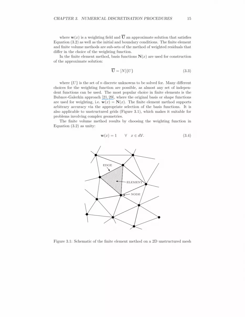
where {U} is the set of n discrete unknowns to be solved for. Many differentchoices for the weighting function are possible, as almost any set of indepen-dent functions can be used. The most popular choice in finite elements is theBubnov-Galerkin approach [21, 29], where the original basis or shape functionsare used for weighting, i.e. w(x) = N(x). The finite element method supportsarbitrary accuracy via the appropriate selection of the basis functions. It isalso applicable to unstructured grids (Figure 3.1), which makes it suitable forproblems involving complex geometries.

The finite volume method results by choosing the weighting function inEquation (3.2) as unity:

w(x) = 1 ∀ x ∈ dV . (3.4)

������������������������������������������������������������������������������������������������������������������������������������������������������������������������������������

������������������������������������������������������������������������������������������������������������������������������������������������������������������������������������EDGE

ELEMENT

NODE

Figure 3.1: Schematic of the finite element method on a 2D unstructured mesh

CHAPTER 3. NUMERICAL DISCRETISATION PROCEDURES 16

���������������������������������������������������������������������������������������������������������������������������������������������������������������������������

���������������������������������������������������������������������������������������������������������������������������������������������������������������������������

FINITE VOLUME

�����������������������������������������������������������������������������������������������������������������������������������������������������������������������������������������������������������������

�����������������������������������������������������������������������������������������������������������������������������������������������������������������������������������������������������������������

FINITE VOLUME

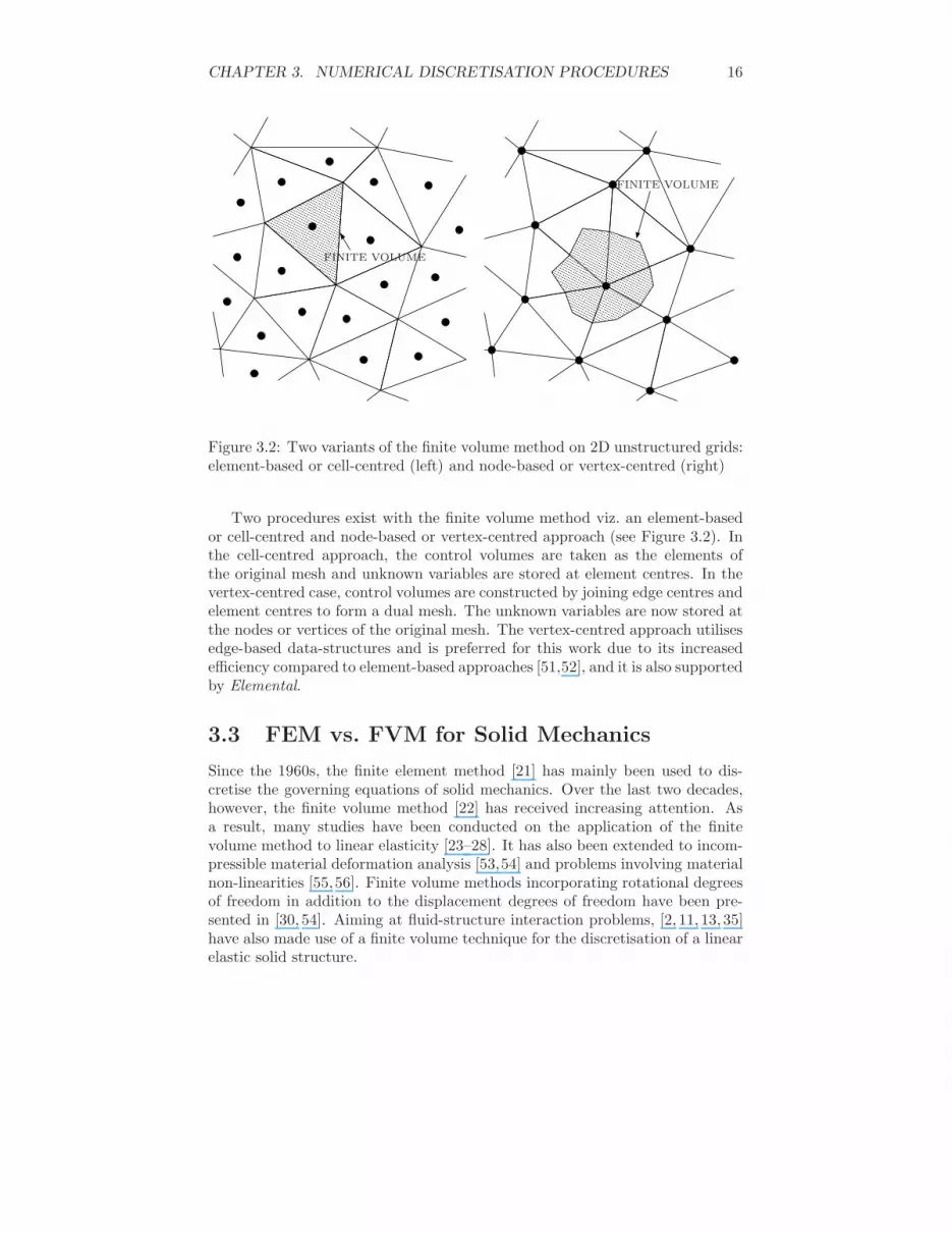
Figure 3.2: Two variants of the finite volume method on 2D unstructured grids:element-based or cell-centred (left) and node-based or vertex-centred (right)

Two procedures exist with the finite volume method viz. an element-basedor cell-centred and node-based or vertex-centred approach (see Figure 3.2). Inthe cell-centred approach, the control volumes are taken as the elements ofthe original mesh and unknown variables are stored at element centres. In thevertex-centred case, control volumes are constructed by joining edge centres andelement centres to form a dual mesh. The unknown variables are now stored atthe nodes or vertices of the original mesh. The vertex-centred approach utilisesedge-based data-structures and is preferred for this work due to its increasedefficiency compared to element-based approaches [51,52], and it is also supportedby Elemental.

3.3 FEM vs. FVM for Solid Mechanics

Since the 1960s, the finite element method [21] has mainly been used to dis-cretise the governing equations of solid mechanics. Over the last two decades,however, the finite volume method [22] has received increasing attention. Asa result, many studies have been conducted on the application of the finitevolume method to linear elasticity [23–28]. It has also been extended to incom-pressible material deformation analysis [53,54] and problems involving materialnon-linearities [55,56]. Finite volume methods incorporating rotational degreesof freedom in addition to the displacement degrees of freedom have been pre-sented in [30, 54]. Aiming at fluid-structure interaction problems, [2, 11, 13, 35]have also made use of a finite volume technique for the discretisation of a linearelastic solid structure.

CHAPTER 3. NUMERICAL DISCRETISATION PROCEDURES 17

It is well known that the linear finite element formulation suffers from sensi-tivity to element aspect ratio or shear locking when subjected to bending [29].Fallah [28] and Wheel [26] present a locking-free finite volume approximation toMindlin-Reissner plates for both cell-centred and vertex-centred formulations.However, using solid elements, Wenke and Wheel [30] present results that doindicate shear locking with the displacement-based vertex-centred finite volumeapproach. Further, Oxtoby et al. [17] developed a displacement-based hybridfinite volume method that holds promise as being locking-free [20]. A morerigorous evaluation of the suitability of the finite volume method for modellinga structure under bending with varying element aspect ratios, is presented inthis work.

When considering geometrically non-linear problems as seen in this work,Fallah et al. [31] presented a finite volume procedure and also compared the re-sults with a finite element method. They concluded that for a low mesh densitythe difference between the finite volume and finite element methods are consid-erable, with the finite element method being more accurate, but by increasingthe number of elements the accuracy of the two methods are comparable. Onthe other hand, Vaz Jr. et al. [32] state that the finite element formulationprovides higher accuracy for displacement solutions. In this work, a rigorouscomparison between the two methods will be made.

For structures under non-linear bending, it is known that at the least cubicdisplacement fields result. Therefore, higher-order methods are also consideredin this work. The finite element Galerkin method uses shape functions as theweighting functions and may be easily extended to higher-order via higher-orderpolynomials for the shape functions [21]. The finite volume method resultsby choosing the weighting function as unity. To the author’s knowledge nohigher-order finite volume method for computational solid mechanics has beenpresented thus far. Such a formulation is therefore developed in this work.

3.4 Spatial Discretisation: Finite Element Method

The standard Galerkin finite element method of discretisation is described inthis section. The strong form of the equilibrium equation written in terms ofthe undeformed configuration, Equation (2.25), in the absence of body forces isgiven by

ρoa = DivP. (3.5)

The equation is cast into weak form based on the method of weighted resid-uals. This is done by first expressing the governing equation as a residual, R,as follows

R = DivP − ρoa. (3.6)

The residual is then dotted with a weighting field, w, and integrated over

CHAPTER 3. NUMERICAL DISCRETISATION PROCEDURES 18

the entire domain, Vo, which renders the equation in weak form∫

Vo

w · RdVo = 0. (3.7)

The weighting field, w, is the set of all possible functions, with the restric-tion that w = 0 along that part of the boundary of the domain where thedisplacement is prescribed, Au.

Expanding the terms in Equation (3.7) gives∫

Vo

w · (DivP− ρoa)dVo = 0 (3.8)

∫

Vo

w · DivPdVo −∫

Vo

ρow · adVo = 0. (3.9)

Using the definition of the divergence of a second order tensor, as well as theproduct rule of differentiation, it can be shown [57] that

Div(PT w) = w · DivP + P · ∂w

∂X. (3.10)

Re-arranging and substituting Equation (3.10) in Equation (3.9) gives∫

Vo

[

Div(PT w)dVo − P · ∂w

∂X

]

dVo −∫

Vo

ρow · adVo = 0 (3.11)

∫

Vo

Div(PT w)dVo −∫

Vo

P · ∂w

∂XdVo −

∫

Vo

ρow · adVo = 0. (3.12)

We now apply Gauss’s Divergence Theorem to the first term on the left-hand-side of Equation (3.12):

∫

Ao

(PT w) · nodAo −∫

Vo

P · ∂w

∂XdVo −

∫

Vo

ρow · adVo = 0 (3.13)

∫

Ao

(Pno) ·wdAo −∫

Vo

P · ∂w

∂XdVo −

∫

Vo

ρow · adVo = 0, (3.14)

where Ao is the boundary surface enclosing Vo and no is the outward pointingunit normal vector.

But, to = Pno [57], where to denotes the surface traction expressed in theundeformed configuration, therefore

∫

Ao

to ·wdAo −∫

Vo

P · ∂w

∂XdVo −

∫

Vo

ρow · adVo = 0. (3.15)

Splitting up the boundary integral into two parts: Au where the displace-ment up is prescribed and At where the surface traction tp

o is prescribed gives∫

At

to · wdAo +

∫

Au

to · wdAo −∫

Vo

P · ∂w

∂XdVo −

∫

Vo

ρow · adVo = 0. (3.16)

CHAPTER 3. NUMERICAL DISCRETISATION PROCEDURES 19

Equation (3.16) is now simplified by noting that w = 0 along Au and alongAt the traction is prescribed, therefore

∫

At

tpo ·wdAo −

∫

Vo

P · ∇XwdVo − ρo

∫

Vo

w · adVo = 0. (3.17)

Equation (3.17) represents the general weak form of the solid mechanicsboundary value problem. There are two interesting facts to note about thisequation. Firstly, the traction boundary condition now appears explicitly withinthe governing equation. Secondly, since we apply this boundary condition Pn =tpo within the integral, this means that the boundary condition is only satisfied

in weak form or in a weighted average sense.Instead of solving for all possible set of weighting functions for w to obtain an

exact solution, we consider only a finite set of functions for w. These functionsare chosen as piecewise-continuous low-order polynomial functions defined onsub-domains (elements) within the total domain Vo and are referred to as basisor shape functions [N ]. The weighting field is now interpolated between nodalweighting values {W} using these shape functions, i.e.

w = [N ] {W}. (3.18)

The primary variable, viz. the displacement field u, is interpolated over anelement using the same shape functions:

u = [N ] {U}, (3.19)

where {U} is the vector containing the nodal displacements. Using the sameshape functions for both the displacement and weighting field is referred to asthe Bubnov-Galerkin method.

Substituting Equations (3.18) and (3.19) into Equation (3.17) and simplify-ing, noting that a = [N ]{U}, gives

∫

At

wT tpodAo −

∫

Vo

(∇Xw)T PdVo = ρo

∫

Vo

aTwdVo (3.20)

∫

At

{W}T [N ]T {tpo}dAo−

∫

Vo

{W}T [B]T {P}dVo = ρo

∫

Vo

{W}T [N ]T [N ]{U}dVo,

(3.21)where [B] is a matrix containing the derivatives of the shape functions and {P}is a vector containing the first Piola-Kirchoff stress. The details of how thismatrix is constructed is discussed in the next section.

Since {W} is arbitrary and not equal to zero, Equation (3.21) can be sim-plified to:

∫

At

[N ]T {tpo}dAo −

∫

Vo

[B]T {P}dVo = ρo

∫

Vo

[N ]T [N ]{U}dVo (3.22)

where {U} contains constant nodal values and can be removed from the integral.

CHAPTER 3. NUMERICAL DISCRETISATION PROCEDURES 20

The domain is discretised into a finite number of non-overlapping controlvolumes or element domains Ve, which are defined in the undeformed configura-tion. Equation (3.22) is now expressed as the sum over all the elements withinthe domain:

∑

e

∫

Aet

[N ]T {tpo}dAo −

∑

e

∫

Ve

[B]T {P}dVo =∑

e

ρo

∫

Ve

[N ]T [N ] dVo{U}.

(3.23)

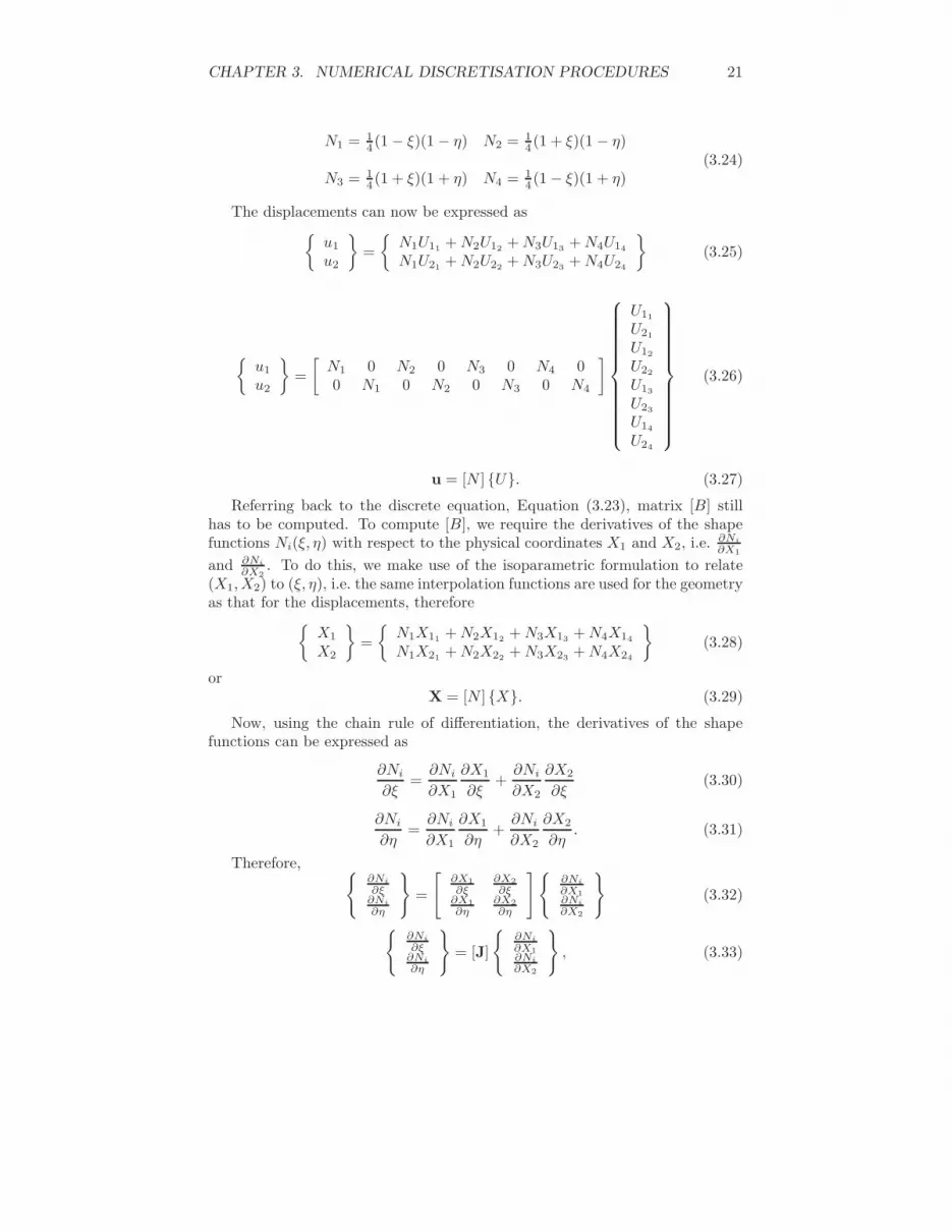
3.4.1 Q4 Finite Element Method

The bilinear quadrilateral or Q4 plane element is described in this section. Inthis form of the finite element method, the domain is discretised into four-nodedisoparametric quadrilateral elements. Figure 3.3 (left) shows an actual Q4 el-ement in physical space. With the isoparametric formulation, the same shapefunctions used to interpolate displacements are also used for interpolating thegeometry. Therefore, isoparametric elements need not be restricted to rectan-gular shapes, making it suitable to be used to mesh complicated geometries.

To facilitate the isoparametric formulation the element is mapped or trans-formed into a reference element. As shown in Figure 3.3 (right), this is doneusing reference or natural coordinates ξ and η. The sides of the reference ele-ment intersect the ξ and η axes at ξ = ±1 and η = ±1, thus making the referenceelement a square of two units width on either side. The point ξ = η = 0 is thecentre of the element.

The Q4 element can only accommodate bilinear polynomials as shape func-tions. These shape functions can be derived intuitively by noting that for anyshape function Ni, Ni = 1 at node i and Ni = 0 at every other node. Followingthis approach, the Q4 shape functions are:

1

1

22

33 4

4

x1

x2

ξ

η

Figure 3.3: Isoparametric Q4 element in physical space (left) and reference space(right)

CHAPTER 3. NUMERICAL DISCRETISATION PROCEDURES 21

N1 = 14 (1 − ξ)(1 − η) N2 = 1

4 (1 + ξ)(1 − η)

N3 = 14 (1 + ξ)(1 + η) N4 = 1

4 (1 − ξ)(1 + η)(3.24)

The displacements can now be expressed as{

u1

u2

}

=

{

N1U11 + N2U12 + N3U13 + N4U14

N1U21 + N2U22 + N3U23 + N4U24

}

(3.25)

{

u1

u2

}

=

[

N1 0 N2 0 N3 0 N4 00 N1 0 N2 0 N3 0 N4

]

U11

U21

U12

U22

U13

U23

U14

U24

(3.26)

u = [N ] {U}. (3.27)

Referring back to the discrete equation, Equation (3.23), matrix [B] stillhas to be computed. To compute [B], we require the derivatives of the shapefunctions Ni(ξ, η) with respect to the physical coordinates X1 and X2, i.e. ∂Ni

∂X1

and ∂Ni

∂X2. To do this, we make use of the isoparametric formulation to relate

(X1, X2) to (ξ, η), i.e. the same interpolation functions are used for the geometryas that for the displacements, therefore

{

X1

X2

}

=

{

N1X11 + N2X12 + N3X13 + N4X14

N1X21 + N2X22 + N3X23 + N4X24

}

(3.28)

orX = [N ] {X}. (3.29)

Now, using the chain rule of differentiation, the derivatives of the shapefunctions can be expressed as

∂Ni

∂ξ=

∂Ni

∂X1

∂X1

∂ξ+

∂Ni

∂X2

∂X2

∂ξ(3.30)

∂Ni

∂η=

∂Ni

∂X1

∂X1

∂η+

∂Ni

∂X2

∂X2

∂η. (3.31)

Therefore,{

∂Ni

∂ξ∂Ni

∂η

}

=

[

∂X1

∂ξ∂X2

∂ξ∂X1

∂η∂X2

∂η

]{

∂Ni

∂X1∂Ni

∂X2

}

(3.32)

{

∂Ni

∂ξ∂Ni

∂η

}

= [J]

{

∂Ni

∂X1∂Ni

∂X2

}

, (3.33)

CHAPTER 3. NUMERICAL DISCRETISATION PROCEDURES 22

where [J] is called the Jacobian matrix and is computed using Equation (3.28)and (3.24).

The required derivatives for the matrix [B] are now computed using theinverse of the Jacobian matrix

{

∂Ni

∂X1∂Ni

∂X2

}

= [J]−1

{

∂Ni

∂ξ∂Ni

∂η

}

. (3.34)

Equation (3.23) now reads

∑

e

{Fext} −∑

e

(∫ 1

−1

∫ 1

−1

[B]T {P}det(J)dξdη

)

=∑

e

ρo

∫

Ve

[N ]T

[N ] dVo{U},

(3.35)where the external loads are simply denoted as {Fext} and det(J) is the de-terminant of the Jacobian matrix and is used to transform the integral in thephysical coordinates to that in the reference coordinates.

Finally, the double spatial integral in Equation (3.35) is computed numeri-cally using Gauss quadrature, i.e. the integral is evaluated at a specific numberof Gauss points, the result is then multiplied by a weighting factor WGP andthe results summed over all the Gauss points

∑

e

{Fext} −∑

e

∑

Gauss pts

[B]T {P}det(J)WGP

=∑

e

ρo

∫

Ve

[N ]T [N ] dVo{U}.

(3.36)

The temporal term on the right-hand-side of the equation is discretised usinga dual-timestepping procedure and is discussed later.

3.4.2 Q8 Finite Element Method

The Q4 element, described in the previous section, is limited to linear shapefunctions within each element. Use of higher-order interpolation may lead tofar more accurate results. For thin structures under non-linear bending as seenin this work, higher-order displacement fields result. As we would like to useas few elements through the thickness as possible, higher-order methods willbe considered. The Q8 finite element formulation is a direct extension of theQ4 approach discussed above. The eight-noded quadrilateral or Q8 element isobtained by adding a mid-node to each side of the Q4 element. These mid-nodesallow the Q8 element to even have curved sides. Figure 3.4 (left) shows a Q8element in the physical space and in the reference space (right).

CHAPTER 3. NUMERICAL DISCRETISATION PROCEDURES 23

1

1

22

33 4

4

5

5

6

6

77

8

8

x1

x2

ξ

η

Figure 3.4: Isoparametric Q8 element in physical space (left) and reference space(right)

The shape functions for the Q8 element contain higher-order quadratic terms:

N1 = −0.25(1− ξ)(1 − η)(1 + ξ + η) N5 = 0.5(1 − ξ2)(1 − η)

N2 = −0.25(1 + ξ)(1 − η)(1 − ξ + η) N6 = 0.5(1 + ξ)(1 − η2)

N3 = −0.25(1 + ξ)(1 + η)(1 − ξ − η) N7 = 0.5(1 − ξ2)(1 + η)

N4 = −0.25(1− ξ)(1 + η)(1 + ξ − η) N8 = 0.5(1 − ξ)(1 − η2),

(3.37)

which are then implemented directly into Equation (3.36).

3.5 Spatial Discretisation: Finite Volume Method

At the commencement of this study, Elemental supported the finite volumeframework. In this section, we now describe the finite volume method of dis-cretising the equations governing solid mechanics. Two variants thereof, thestandard vertex-centred approach and the hybrid finite volume approach, bothsupported by Elemental, are implemented. We then extend the finite volumemethod to a higher-order accurate formulation.

Consider again the equilibrium equation, Equation (2.25):

ρoa = DivP + bo. (3.38)

For the purposes of discretisation, the equation above is re-written in indicialnotation as

ρoai =∂PiJ

∂XJ

+ boI . (3.39)

Assuming the body forces, boI , to be negligible and expressing the accelera-

tion, ai, as the rate of change of velocity, vi, gives

CHAPTER 3. NUMERICAL DISCRETISATION PROCEDURES 24

ρo

∂vi

∂t=

∂PiJ

∂XJ

. (3.40)

As per the finite element method, discretisation commences by casting theequation into integral or weak form by integrating over an arbitrary spatialsubdomain Vm in the reference (undeformed) configuration:

∫

Vm

ρo

∂vi

∂tdVo =

∫

Vm

∂PiJ

∂XJ

dVo. (3.41)

The control volume, Vm, is fixed in time, therefore differentiation and inte-gration of the temporal term are interchangeable. In addition, ρo is constant,so the left-hand-side of the equation simplifies to

ρo

d

dt

∫

Vm

vidVo =

∫

Vm

∂PiJ

∂XJ

dVo. (3.42)

Applying the Divergence Theorem of Gauss, the spatial derivative may bewritten in terms of fluxes as:

ρo

d

dt

∫

Vm

vidVo =

∮

Am

PiJ · nJdAo (3.43)

where Am is the surface enclosing Vm and n = (n1, n2) is the outward pointingunit-vector normal to Am.

3.5.1 Vertex-centred Finite Volume Method

A vertex-centred finite volume approach utilising edge-based data-structureswas selected over an element-based approach for use in Elemental, due to itsincreased computational efficiency [51, 52] and suitability for computation ondistributed memory parallel hardware architectures. In the edge-based vertex-centred method, the dependent variables are stored at nodes around which con-trol volumes are constructed. In 2D, these control volumes are constructed byjoining the midpoints of edges with element centroids and in such a way thatonly one node lies within each control volume. The set of surfaces forming thecontrol volumes are referred to as a dual-mesh. This is shown schematically fora node m in Figure 3.5 [15]. In the figure, Vm is the control volume associatedwith node m. Its bounding surface Am is composed of a number of surfaceswhich are defined based on their associated edges. For example, Amn is thesurface segment intersecting the edge Υmn which connects nodes m and n.

The surface integrals in Equation (3.43) are now calculated in an edge-wisemanner, i.e. the surface integral is expressed as the sum over all the edgesconnecting the control volume

ρo

d

dt

∫

Vm

vidVo =∑

Υmn∩Vm

PiJ · CJ:mn, (3.44)

CHAPTER 3. NUMERICAL DISCRETISATION PROCEDURES 25

where Cmn is the edge-coefficient for an internal edge Υmn. An edge-coefficientis defined as the area of the bounding surface of a particular edge in a con-trol volume multiplied by the outward pointing unit-vector normal to its face;therefore

CJ:mn =∑

Amnt∈Amn

nJ:mntAmnt

(3.45)

where Amntis a segment of the surface Amn and nJ:mnt

is the unit-vectornormal to Amnt

. For the edge Υmn shown in Figure 3.5, the edge-coefficient iscomprised of two surfaces t = 1 and t = 2.

The surfaces of some control volumes of the dual-mesh may lie on the bound-ary of the domain, denoted by AmB

in Figure 3.5.Equation (3.44) is therefore updated to include the domain boundary edges

ρo

d

dt

∫

Vm

vidVo =∑

Υmn∩Vm

PiJ · CJ:mn +∑

ΥBmn∩Vm

PiJ · BJ:mn. (3.46)

Boundary edge-coefficients are computed in a similar way to their internaledge counterparts:

BJ:mn =∑

AmnBt

∈AmnB

nJ:mnBtAmn

Bt (3.47)

where nJ:mnBq is the outward pointing unit-vector normal to the boundary sur-face segment AmnBq . For the case shown in Figure 3.5, Υmp is a boundary edge

Amn

Amn1Amn2

Amp

AmpBApmB

Υmn

m

n

p

Vm

Am

AmB

Figure 3.5: Schematic of the construction of a dual-mesh

CHAPTER 3. NUMERICAL DISCRETISATION PROCEDURES 26

and AmpBis the domain boundary surface associated with this edge. Therefore,

for a 2D domain as above, t is always equal to 1 in Equation (3.47).Displacement gradients are evaluated numerically at the nodes or vertices.

Therefore, referring to Figure 3.5 and following from Gauss’s divergence theo-rem, the displacement gradients for node m are given by:

∂ui

∂XJ

∣

∣

∣

∣

m

=1

Vm

∮

Am

ui · nJdAm =1

Vm

∑

Υmn∩Vm

(

ui:mn · CJ:mn

)

(3.48)

where ui:mn is the linearly-interpolated displacement at the face:

ui:mn ≈ 1

2(ui:m + ui:n). (3.49)

In the edge-based procedure, the stresses are calculated at the faces of thedual-cells using a compact stencil [58, 59]. The displacement gradients at thefaces are therefore given by:

∂ui

∂XJ

∣

∣

∣

∣

mn

≈ ui:n − ui:m

|l|lj

|l| +1

2

(

∂ui

∂XJ

∣

∣

∣

∣

m

+∂ui

∂XJ

∣

∣

∣

∣

n

)∣

∣

∣

∣

normal

(3.50)

where l is the edge-length and |normal indicates the component in the directionnormal to the edge.

The strains evaluated using Equations (2.32) and (2.33) and these displace-ment gradients are referred to as node-based strains. Finally, the stresses, re-quired to evaluate the integrals in Equation (3.46), are computed using Equa-tions (2.26) and (2.31).

3.5.2 Hybrid Finite Volume Method

In the vertex-centred finite volume method described above, displacement gradi-ents are evaluated at the nodes or vertices. This is different to the conventionalfinite element method, where stresses are evaluated at integration points withinthe element [29]. An alternative to the finite volume method just describedwhere displacement gradients are evaluated at element centres, as proposedin [14], is considered. This is equivalent to the finite element method with oneintegration point.

Referring to Figure 3.6, the displacement gradients for element M are givenby:

∂ui

∂XJ

∣

∣

∣

∣

M

=1

VM

∑

ΥM∩VM

(

ui:MN · nJ:MNAMN

)

(3.51)

where AMN is the surface segment between elements M and N and ui:MN isthe linearly-interpolated displacement of this surface (note that in 2D ui:mn andui:MN are identical):

ui:MN ≈ 1

2(ui:m + ui:n). (3.52)

CHAPTER 3. NUMERICAL DISCRETISATION PROCEDURES 27

m

n

M

N

VM

VN

AMN

ΥM

Figure 3.6: Schematic of a mesh showing the calculation of element-based gra-dients

The displacement gradients at the faces are obtained by averaging theirvalues between the two connecting elements:

∂ui

∂XJ

∣

∣

∣

∣

mn

≈ 1

2

(

∂ui

∂XJ

∣

∣

∣

∣

M

+∂ui

∂XJ

∣

∣

∣

∣

N

)

. (3.53)

The strains evaluated using these displacement gradients are referred to aselement-based strains.

A finite volume approach using only element-based strains suffers from odd-even decoupling as displacements appear only in the combination (ui:m + ui:n).A hybrid finite volume method to remedy the odd-even decoupling was proposedin [17, 20]. This method uses element-based strains for the shear components,but node-based strains for the normal components. Therefore, Equation (3.53)is used for the displacement gradients in Eij with i 6= j and Equation (3.50)in Eij with i = j. This is similar to the selective integration approach [29]used in the finite element method to eliminate spurious modes, where differentGauss quadrature integration rules are used for the shear and normal straincontributions to the stiffness matrix.

Consequently, both the vertex-centred FVM, which uses only node-basedstrains, and the hybrid FVM, which uses a combination of node- and element-based strains, were implemented in this work.

3.5.3 Proposed Higher-Order Finite Volume Method

As discussed above, higher-order methods are common with the finite elementmethod by using higher-order polynomials for the shape functions. However,with the finite volume method the weighting function is set equal to unity andthe same approach to develop a higher-order finite volume method cannot beused. Instead, an error analysis is conducted on the vertex-centred and hy-

CHAPTER 3. NUMERICAL DISCRETISATION PROCEDURES 28

brid finite volume formulations and using this information, a higher-order finitevolume formulation is then developed.

Error Analysis: Analytical Approach

In this section, a detailed error analysis is conducted analytically on both thevertex-centred and hybrid finite volume formulations (the detailed derivationsare included in Appendix A). To simplify the error analysis, we limit the prob-lem to the small displacement case. Consider again the governing equation,Equation (2.25):

ρai =∂σij

∂xj

+ bi (3.54)

where σij is the stress. Note that in the small displacement case the Cauchyand Piola-Kirchoff stress are identical and will simply be denoted by σij .

Since we are only interested in the spatial accuracy, we neglect the temporalterm and consider only the steady-state problem, i.e. ai = 0. With body forces,bi, negligible, the equation simplifies to:

∂σij

∂xj

= 0. (3.55)

Numerical error is introduced by discretisation, which can be expressed by:

∑

Υmn∩Vm

σij · Cj:mn +∑

ΥBmn∩Vm

σij · Bj:mn =∂σij

∂xj

∣

∣

∣

∣

m

+ Errori:m. (3.56)

The exact form of this Errori:m term may be determined analytically. As-suming a Poisson’s ratio of zero, which simplifies the mathematical analysis byeliminating the effect of a loading in the perpendicular or transverse directionyet still provides a qualitative representation of the error terms, the stress-strainrelationship, Equation (2.26), simplifies to:

σij = Eεij . (3.57)

The strain-displacement relationship for the small displacement case is:

εij =1

2

(

∂ui

∂xj

+∂uj

∂xi

)

. (3.58)

Substituting Equation (3.57) and Equation (3.58) into Equation (3.56) givesan equation expressed in terms of displacements, from which the numericalerrors can be determined.

In this work only structured equi-spaced meshes are considered for the solid,which further simplifies the analysis. Consider first the standard vertex-centredformulation for the case of an internal node (Figure 3.7(a)). Substituting theexpressions for the displacement gradients, Equation (3.50), and expanding eachterm using Taylor series expansions about the node, the discrete expression for

CHAPTER 3. NUMERICAL DISCRETISATION PROCEDURES 29

(a)

(b) (c)

∆x1∆x2

Figure 3.7: Schematic of the mesh indicating an internal, boundary and cornernode

the leading error-term at an internal node (see Appendix A for the details ofthis derivation) is given by:

Errori =E

2

(

1

6

∂4ui

∂x4i

∆x2i +

1

12

∂4ui

∂x4k

∆x2k +

1

6

∂4uk

∂x3i ∂xk

∆x2i +

1

6

∂4uk

∂xi∂x3k

∆x2k

)

(3.59)with

i = 1; k = 2 for the x1-momentum equation

i = 2; k = 1 for the x2-momentum equation.

Similarly, for a boundary node (Figure 3.7(b)) the leading-order error termsfor the tangential and normal components of the momentum equations, respec-tively, are (see Appendix A for the detailed derivation):

Errort =E

2

(

1

6

∂4ut

∂x4t

∆x2t +

1

3

∂3ut

∂x3n

∆xn + (−1)p 1

2

∂3un

∂xt∂x2n

∆xn+

(−1)p 1

3

∂3un

∂x3t

∆x2t

∆xn

)

(3.60)

Errorn =E

2

(

(−1)p 1

2

∂3ut

∂xt∂x2n

∆xn

)

(3.61)

where subscripts n and t denote coordinates normal and tangential to the bound-ary respectively, p = 1 for the top and right boundaries and p = 2 for the bottomand left boundaries.

Finally, for a corner node (Figure 3.7(c)) the leading-order error term is (seeAppendix A for the detailed derivation):

Errori =E

2

(

(−1)p ∂2uk

∂x2i

∆xi

∆xk

)

(3.62)

CHAPTER 3. NUMERICAL DISCRETISATION PROCEDURES 30

withi = 1; k = 2 for the x1-momentum equation

i = 2; k = 1 for the x2-momentum equation

p = 1 for the top-left and bottom-right corners

p = 2 for the top-right and bottom-left corners.

Two important conclusions can be derived from the leading-order error termsfor the standard vertex-centred formulation above. Firstly, the truncation error

is of order O(∆x2i )+O(∆x2

k) at internal nodes, O(∆xn)+O(∆x2

t

∆xn) at boundary

nodes and O( ∆xi

∆xk) at corner nodes. Therefore, second-order rate of convergence

is expected for internal nodes but only first-order for boundary nodes and zero-order for corner nodes. In addition, since the coefficients of the leading-ordererror terms at internal nodes are fourth-order derivatives, the formulation will beexact at internal nodes for a displacement field described by a cubic polynomial.However, at boundary nodes the formulation can only represent quadratic fieldsexactly and similarly only linear fields at corner nodes.

Using the same approach for the hybrid formulation, but substituting Equa-tion (3.53) for the displacement gradients in Eij with i 6= j and Equation (3.50)in Eij with i = j, the leading-order error term at the internal node (Fig-ure 3.7(a)) is (see Appendix A for the detailed derivation):

Errori =E

2

(

1

6

∂4ui

∂x4i

∆x2i +

1

12

∂4ui

∂x4k

∆x2k +

1

6

∂4uk

∂x3i ∂xk

∆x2i +

1

6

∂4uk

∂xi∂x3k

∆x2k +

1

4

∂4ui

∂x2i ∂x2

k

∆x2i

)

(3.63)

where the nomenclature is as previously defined.For a boundary node (Figure 3.7(b)) (see Appendix A for the detailed deriva-

tion):

Errort =E

2

(

1

6

∂4ut

∂x4t

∆x2t +

1

3

∂3ut

∂x3n

∆xn + (−1)p 1

2

∂3un

∂xt∂x2n

∆xn+

(−1)p 1

3

∂3un

∂x3t

∆x2t

∆xn

+ (−1)q ∂3ut

∂x2t ∂xn

∆x2t

∆xn

)

(3.64)

Errorn =E

2

(

(−1)p 1

2

∂3ut

∂xt∂x2n

∆xn + (−1)q 1

2

∂3un

∂x2t ∂xn

∆xn

)

(3.65)

where q = 1 for the left and right boundaries and q = 2 for the bottom and leftboundaries and the rest of the symbols are as previously defined.

Finally, for a corner node (Figure 3.7(c)) the leading-order error term is (seeAppendix A for the detailed derivation):

Errori =E

2

(

(−1)p ∂2uk

∂x2i

∆xi

∆xk

− ∂2ui

∂xi∂xk

∆xi

∆xk

)

. (3.66)

CHAPTER 3. NUMERICAL DISCRETISATION PROCEDURES 31

Vertex-centred FVM Hybrid FVM

Internal node O(∆x2i ) + O(∆x

2k) 2nd-order O(∆x

2i ) + O(∆x

2k) 2nd-order

Boundary node O(∆xn) + O(∆x2

t

∆xn) 1st-order O(∆xn) + O(

∆x2t

∆xn) 1st-order

Corner node O( ∆xi

∆xk) zero-order O( ∆xi

∆xk) zero-order

Table 3.1: Order of accuracy of the vertex-centred and hybrid formulations

The truncation errors of the hybrid formulation are compared with that ofthe vertex-centred formulation in Table 3.1. As can be seen in the table, theseerrors are of the same order for both formulations. Furthermore, based on thecoefficients of the leading-order error terms, the hybrid formulation indicatesthe same order of accuracy as that of the vertex-centred formulation. However,additional terms are present in the error expressions for the hybrid formulationthat may cancel out for specific displacement fields. These will be analysed onspecific test-cases in Chapter 4.

Higher-Order Finite Volume Method

In the previous section, it was shown that both the vertex-centred and hybridfinite volume formulations can represent cubic displacement fields exactly atinternal nodes. However, only quadratic and linear fields are exact at boundaryand corner nodes respectively. For thin structures under linear bending, itis known that at the least cubic displacement fields result. In this section, wedevelop a higher-order finite volume formulation for the small displacement casethat does not suffer from a deterioration in accuracy along the boundaries, i.e.it can represent a third-order displacement field exactly at internal as well asboundary and corner nodes.

With the standard finite volume method the displacement gradients are com-puted in an edge-based manner (see Appendix A for details). A first attemptat developing a higher-order method involved computing these displacementgradients using third-order approximations. However, with the edge-based pro-cedure the derivatives of stress in the momentum equations are computed usingan equivalent forward-difference method at boundary nodes, as opposed to acentral-difference method at internal nodes, hence the formulation always re-mains first-order accurate. Therefore, an approach that uses the traction bound-ary condition explicitly to solve for the displacements along the boundaries wasused.

The traction boundary condition is stated as:

σn = tp (3.67)

or in indicial notation in terms of force:

Fi = σijCj:mn (3.68)

where the nomenclature is as previously defined.

CHAPTER 3. NUMERICAL DISCRETISATION PROCEDURES 32

(x1, x2)

∆x1∆x2

Figure 3.8: Schematic of the mesh indicating a boundary node

Consider a node along a boundary at the bottom of the beam as shown inFigure 3.8.

Expanding Equation (3.68) for this node gives:

F1 = σ11(An1) + σ12(An2) = 0 (3.69)

andF2 = σ21(An1) + σ22(An2) = 0 (3.70)

with(n1, n2) = (0,−1). (3.71)

Substituting the stress-strain and strain-displacement relationships gives twoequations from which the two displacements at the boundary node are solved:

∂u1

∂x2

∣

∣

∣

∣

(x1,x2)

+∂u2

∂x1

∣

∣

∣

∣

(x1,x2)

= 0 (3.72)

∂u2

∂x2

∣

∣

∣

∣

(x1,x2)

= 0. (3.73)

Now, the displacement gradients above are discretised using third-order ap-proximations, e.g. (see Appendix B for details of this derivation):

∂u1

∂x2

∣

∣

∣

∣

(x1,x2)

≈−11u1(x1,x2)

+ 18u1(x1,x2+∆x2)− 9u1(x1,x2+2∆x2)

+ 2u1(x1,x2+3∆x2)

6∆x2

(3.74)where it can be shown that the leading-order error term for this approximationis:

Error = −1

4

∂4u1

∂x42

∆x32. (3.75)

Therefore, this approximation is third-order accurate. Similarly:

∂u2

∂x1

∣

∣

∣

∣

(x1,x2)

≈−3u2(x1,x2)

+ 6u2(x1+∆x1,x2)− u2(x1+2∆x1,x2)

− 2u2(x1−∆x2,x2)

6∆x1

(3.76)

CHAPTER 3. NUMERICAL DISCRETISATION PROCEDURES 33

(x1, x2)

∆x1

∆x2

Figure 3.9: Schematic of the mesh indicating a corner node

∂u2

∂x2

∣

∣

∣

∣

(x1,x2)

≈−11u2(x1,x2)

+ 18u2(x1,x2+∆x2)− 9u2(x1,x2+2∆x2)

+ 2u2(x1,x2+3∆x2)

6∆x2.

(3.77)Equations (3.74), (3.76) and (3.77) are substituted into Equations (3.72)

and (3.73) and the two equations are solved for displacements u1 and u2.Similarly, for a corner node as shown in Figure 3.9, the displacement gradi-

ents are given by:

∂u1

∂x1

∣

∣

∣

∣

(x1,x2)

≈11u1(x1,x2)

− 18u1(x1−∆x1,x2)+ 9u1(x1−2∆x1,x2)

− 2u1(x1−3∆x1,x2)

6∆x1

(3.78)∂u2

∂x2

∣

∣

∣

∣

(x1,x2)

≈−11u2(x1,x2)

+ 18u2(x1,x2+∆x2)− 9u2(x1,x2+2∆x2)

+ 2u2(x1,x2+3∆x2)

6∆x2.

(3.79)A similar approach is followed for the remaining boundaries and corners

giving a higher-order finite volume formulation that can model a third-orderdisplacement field exactly.

3.6 Temporal Discretisation and Solution Pro-

cedure

The temporal term in Equations (3.43) and (3.23) is discretised using a dual-timestepping solution procedure [60,61], such that second-order temporal accu-racy is achieved and the equations are solved in a matrix-free iterative process.

The dual-timestepping procedure is independent of the spatial discretisationstrategy employed, viz. finite volume or finite element. For the finite volumemethod, Equation (3.46), the spatial terms are grouped together and the equa-tion re-written as follows:

ρo

d

dt

∫

Vm

vidVo =∑

Υmn∩Vm

PiJ · CJ:mn +∑

ΥBmn∩Vm

PiJ · BJ:mn (3.80)

CHAPTER 3. NUMERICAL DISCRETISATION PROCEDURES 34

ρoVm

dvi

dt= RHSi (3.81)

where the subscript m indicates the node number and i the component in thex1- or x2-direction.

Now, a pseudo-time temporal term is added to the left-hand-side of theequation and the real-time temporal term added as a source term to the right-hand-side of the equation. Equation (3.81) becomes

ρo

dvi

dτVm = RHSi − ρo

dvi

dtVm. (3.82)

The solution is driven to pseudo-steady state, i.e. dvi

dτ= 0, which makes

Equations (3.81) and (3.82) equivalent and also implies that the actual governingequations are solved in an implicit fashion.

Since the accuracy of the pseudo-time temporal term is of little consequence,as it becomes zero upon convergence, it is discretised to first-order accuracywhile the real-time temporal term is discretised to second-order accuracy, giving

ρo

vτ+∆τi − vτ

i

∆τVm ≈ RHSi − ρo

3vτ+∆τi − 4vn

i + vn−1i

2∆tVm (3.83)

where ∆t is the real-timestep size and ∆τ the pseudo-timestep size.For the finite element method, applying the same dual-timestepping proce-

dure as above to Equation (3.36) gives

∑

e

ρo

∫

Ve

[N ]T

[N ] dVo

d{vi}dt

=∑

e

{Fext} −∑

e

∑

Gauss pts

[B]T [P ]det(J)WGP

(3.84)

∑

e

[Me]consd{vi}

dt= RHSi, (3.85)

where [Me]cons = ρo

∫

Ve[N ]

T[N ] dVo is the element consistent mass matrix.

Therefore, the nodal mass in the finite volume method, Equation (3.81), isnow replaced by an element mass matrix in the finite element method, Equa-tion (3.85).

For the bilinear Q4 element the shape functions are given by Equation (3.24),therefore using 2× 2 Gauss quadrature integration yields the following elementconsistent mass matrix:

[Me]Q4cons =ρoVe

36

4 2 1 22 4 2 11 2 4 22 1 2 4

. (3.86)

CHAPTER 3. NUMERICAL DISCRETISATION PROCEDURES 35

Similarly, the Q8 element consistent mass matrix is:

[Me]Q8cons =ρoVe

108

2 0 1 0 −2 −4 −4 −20 2 0 1 −2 −2 −4 −41 0 2 0 −4 −2 −2 −40 1 0 2 −4 −4 −2 −2−2 −2 −4 −4 16 12 8 12−4 −2 −2 −4 12 16 12 8−4 −4 −2 −2 8 12 16 12−2 −4 −4 −2 12 8 12 16

. (3.87)

Adding a pseudo-time temporal term and treating the real-time temporalterm as a source term gives

∑

e

[Me]lumpedd{vi}dτ

= RHSi −∑

e

[Me]consd{vi}

dt, (3.88)

where [Me]lumped is the diagonal element lumped mass matrix, obtained byplacing particle masses on the diagonals or at nodes. The advantage of usingthe lumped mass matrix for the pseudo-time temporal term is less computationalstorage and processing time, as the equations are uncoupled and solved in anexplicit matrix-free manner.

To obtain the lumped mass matrix for the Q4 element, a simple row summa-tion method was used [21], where contributions of the consistent mass matrixare summed over all the columns and lumped on the diagonal of the lumpedmass matrix:

[Me]Q4lumped=

ρoVe

36

9 0 0 00 9 0 00 0 9 00 0 0 9

. (3.89)

However, for the Q8 element, a lumped mass matrix using the row sum-mation method proved to be unstable for certain cases and the HRZ lumpingapproach [29] was required:

[Me]Q8lumped=

ρoVe

36

1 0 0 0 0 0 0 00 1 0 0 0 0 0 00 0 1 0 0 0 0 00 0 0 1 0 0 0 00 0 0 0 8 0 0 00 0 0 0 0 8 0 00 0 0 0 0 0 8 00 0 0 0 0 0 0 8

. (3.90)

To introduce the primary variable, displacement, into the equation, we sim-ply note that velocity is the temporal rate of change of displacement, ui,

dui

dt= vi. (3.91)

CHAPTER 3. NUMERICAL DISCRETISATION PROCEDURES 36

Discretising the displacement equation using the same approach as for ve-locity above, gives

uτ+∆τi − uτ

i

∆τ≈ vτ+∆τ

i − 3uτ+∆τi − 4un

i + un−1i

2∆t. (3.92)

The solution procedure involves solving for velocity vi and displacement ui

in an iterative fashion. In order to ensure stability for all cases, a second-orderaccurate single-step procedure [21] is employed as follows:

1. At timestep n + 1, loop over all nodes i and set uτi = un

i and vτi = vn

i .

2. Calculate a projected displacement by discretising Equation (3.91) as fol-lows:

uτi = uτ

i + ∆τ

(

vτi − 3uτ+∆τ

i − 4uni + un−1

i

2∆t

)

. (3.93)

3. Using uτi , compute the strain field using Equations (2.32) and (2.33) and

the stress field using Equations (2.26) and (2.31).

4. Solve for vτ+∆τi explicitly using the discretised form of the equilibrium

equations, Equation (3.83) for the finite volume method and Equation (3.88)for the finite element method.

5. Update the displacement at τ + ∆τ using the latest velocity vτ+∆τi and

the acceleration, calculated in step 3, i.e.

uτ+∆τi = uτ

i + ∆τ

(

vτ+∆τi − 3uτ+∆τ

i − 4uni + un−1

i

2∆t

)

+

1

2∆τ2 1

ρoVm

(

RHSi|uτi− ρo

3vτ+∆τi − 4vn

i + vn−1i

2∆tVm

)

. (3.94)

6. The residuals of the equilibrium equation are calculated, Resi = vτ+∆τi −

vτi .

7. The overall residual is calculated from the root mean square of that ateach node, therefore Res =

√∑n

i (Resi)2/n, where n is the number ofnodes.

8. If the residuals are greater than the convergence tolerance, Steps 2 to 5are repeated.

9. If the residuals are less than the convergence tolerance, vτ+∆τi ≈ vτ

i , andthe real-timestep is terminated. Therefore, vn+1

i = vτ+∆τi and un+1

i =uτ+∆τ

i . The next timestep is entered by proceeding to Step 1.

The dual-timestepping procedure, described above for both the finite volumeand finite element methods, is explicit in pseudo-time, which means it is aconditionally stable scheme and a limit exists on the pseudo-timestep size ∆τ .

CHAPTER 3. NUMERICAL DISCRETISATION PROCEDURES 37

The procedure is implicit in real-time, thus the scheme is stable for any choiceof the real-timestep size ∆t.

A stable solution process exists if ∆τ < ∆τcr, where ∆τcr is the criticaltimestep size [21] defined by the following expression:

∆xi

∆τcr>

√

K

ρo

+

√

G

ρo

(3.95)

where ∆xi is the effective mesh spacing in the i-direction and K and G are thebulk and shear modulus,

K =E

3(1 − 2ν), (3.96)

G =E

2(1 + ν). (3.97)

A further limitation exists in that ∆τ must be less than ∆t, therefore theactual pseudo-timestep size is chosen such that:

∆τactual = ∆τcr

[

1 +3

2

∆τcr

∆t

]−1

, (3.98)

where the nomenclature is as previously defined.

3.7 Conclusion

In this chapter, the method of weighted residuals was discussed. Although thefinite element method (FEM) is more common for computational solid mechan-ics (CSM), the finite volume method (FVM) is receiving increased attentionfor this purpose. However, not much work has been done with the FVM forstructures undergoing geometrically non-linear deformations. Furthermore, norigorous comparison between the FVM and FEM is available in the literature.

In this work, both the FVM and FEM of discretisation, and variants thereof,were employed to spatially discretise the governing equations. In particular, alinear Q4 FEM and higher-order Q8 FEM, as well as a vertex-centred FVM andhybrid FVM were implemented. A detailed error analysis was conducted on thefinite volume methods and a higher-order FVM developed. An implicit matrix-free second-order accurate dual-timestepping temporal discretisation procedurewas employed. The accuracy of all these schemes is evaluated in the next chap-ter, via application to a number of test problems.

Chapter 4

Numerical Results and

Evaluation

4.1 Introduction

The previous chapter detailed the mathematical description of the finite vol-ume (FVM) and finite element (FEM) methods for discretising the equationsgoverning geometrically non-linear solid mechanics. Three finite volume meth-ods were described: a vertex-centred or nodal method, a recently developedhybrid method and a newly developed higher-order method. With regards tofinite element methods, standard linear Q4 elements and higher-order Q8 ele-ments were detailed. In this chapter, the accuracy of the schemes are evaluatedin a rigorous manner via application to 2D test problems with increasing de-gree of complexity. This serves to identify the preferred method for modellingthin geometrically non-linear structures, which will be used for fluid-structureinteraction modelling.

4.2 Uniaxial Tension

The first test problem considered was that of a 2D body in uniaxial tension,shown in Figure 4.1. The solid has a Young’s modulus of E = 210 GPa, Poisson’sratio ν = 0.3 and a length and width of 1 mm. Plane strain was assumed in theanalysis. The mesh consisted of a single cell.

The normal stress, σ11, from the finite volume and finite element formula-tions are plotted against tip displacement, c, in Figure 4.2. The formulationsgive exactly the same results. Furthermore, it can be seen that the geometricallynon-linear formulation was implemented correctly, since the σ11 stress increaseslinearly with an increase in c for small displacements, but deviates from thelinear elasticity behaviour at larger displacements. This is expected since atlarge displacements there is a geometric decrease in cross-section that results in

38

CHAPTER 4. NUMERICAL RESULTS AND EVALUATION 39

Figure 4.1: Solid body in uniaxial tension

0 0.01 0.02 0.03 0.04 0.05 0.06 0.07 0.08 0.09 0.10

0.5

1

1.5

2

2.5

3x 10

4

Displacement (mm)

Str

ess

(MP

a)

Linear elasticityFEM: Non−linear elasticityFVM: Non−linear elasticity

Figure 4.2: Comparison of σ11 stress for uniaxial tension

an increase in stress.

4.3 Simple Shear

A 2D body subjected to the deformation

x1 = X1 + cX2 (4.1)

x2 = X2, (4.2)

which results in the body undergoing simple shear as shown in Figure 4.3,was considered next. The same geometry, mesh and material properties as theprevious case, were used.

Both the σ11 and σ12 stress components are plotted against tip displacement,c, in Figure 4.4. Again, the finite volume and finite element non-linear elasticityformulations give exactly the same results. The linear elasticity formulation pre-dicts zero normal stress components and the shear stress, σ12, increases linearly

CHAPTER 4. NUMERICAL RESULTS AND EVALUATION 40

with an increase in c. Using the non-linear formulations, all the stress terms arenon-zero. The reason for this is due to the overly constrained structure, whichwants to contract in the x1-direction due to the shear stress but the constraints,however, do not allow for this contraction. This results in a strain in the x2-direction and because of the Poisson effect this strain results in normal stresscomponents, σ11 and σ22.

X1

X2

Figure 4.3: Solid body in simple shear

0 0.01 0.02 0.03 0.04 0.05 0.06 0.07 0.08 0.09 0.1−1000

0

1000

2000

3000

4000

5000

6000

7000

8000

9000

Displacement (mm)

Str

ess

(MP

a)

Linear elasticityFEM: Non−linear elasticityFVM: Non−linear elasticity

σ12

σ11

Figure 4.4: Comparison of σ11 and σ12 stress for simple shear

CHAPTER 4. NUMERICAL RESULTS AND EVALUATION 41

4.4 Pure Bending

The next test-case considered was that of a thin beam in pure bending, Fig-ure 4.5. The beam was clamped at one end and subjected to a moment at thefree end. The material properties used were a Young’s modulus E = 210 GPaand Poisson’s ratio ν = 0. The length l = 6 mm, height h = 1 mm and theplane stress assumption were used.

M

Figure 4.5: Cantilever beam in pure bending

A linear elastic solid model was used for this problem. The analytical solu-tion for the displacement of the beam can be derived from first principles andis given by

u1 =Mx1x2

EI(4.3)

u2 = −Mx21

2EI, (4.4)

where u1 and u2 are the displacements in the x1− and x2−directions respec-tively, M is the bending-moment at the free end and I is the moment of inertiaof the cross-section of the beam.

Meshes with varying element aspect ratios, as shown in Figure 4.6, were usedto analyse this problem. The element aspect ratio is defined as the ratio of theelement length to its height. Note that the number of elements in each meshwere chosen so that by keeping the total number of elements constant, varyingaspect ratios could be obtained.

The resulting tip displacements when using the linear four-node (Q4) andhigher-order eight-node (Q8) finite element formulations are shown in Fig-ure 4.7(a), together with the analytical solution. While the Q8 FEM is exact, thewell known shear locking phenomenon [29] is evident with the Q4 FEM. Whensubjected to pure bending, Q4 elements produce a shear strain contribution inaddition to the expected bending strain. This parasitic shear strain absorbsstrain energy and to compensate the displacements decrease or the structurestiffens or locks. This shear locking effect is magnified when the aspect ratiois increased, i.e. as the elements become long and thin, the structure becomesstiffer and results in decreasing displacements. This effect can clearly be seenin Figure 4.7(a).

CHAPTER 4. NUMERICAL RESULTS AND EVALUATION 42

(a) Aspect ratio = 1 (b) Aspect ratio = 4

(c) Aspect ratio = 9 (d) Aspect ratio = 36

Figure 4.6: Meshes with varying element aspect ratios used for analysing a beam in pure bending

The results from the three finite volume formulations are shown in Fig-ure 4.7(b). The vertex-centred FVM also suffers from shear locking. The hy-brid and higher-order FVM are, however, locking-free, with both predicting theexact tip displacement for this problem.

4.4.1 Error Analysis: Application to Beam in Pure Bend-

ing

The analytical solution for the displacement of a beam in pure bending is givenby Equations (4.3) and (4.4). Since it is a quadratic displacement field, it is ex-

CHAPTER 4. NUMERICAL RESULTS AND EVALUATION 43

0 5 10 15 20 25 30 35 400

0.2

0.4

0.6

0.8

1

1.2x 10

−3

Aspect ratio

Dis

plac

emen

t

FEM: Q4FEM: Q8Analytical

(a)

0 5 10 15 20 25 30 35 400

0.2

0.4

0.6

0.8

1

1.2x 10

−3

Aspect ratio

Dis

plac

emen

t

FVM: VertexFVM: HybridFVM: Higher−order

(b)

Figure 4.7: Tip displacement as a function of element aspect ratio: (a) Q4 and Q8 FEM; (b) vertex-centred,hybrid and higher-order FVM

pected that the Q8 FEM and higher-order FVM are exact. The hybrid FVM’ssuperiority over the Q4 FEM and vertex-centred FVM is an interesting finding.As shown in Chapter 3, both the hybrid and vertex-centred formulation shouldcontain error terms at the corners. To understand the difference in accuracybetween the two formulations, the exact errors can be obtained by substitut-ing the analytical solution into the expressions for the errors, Equations (3.59)to (3.66). These are summarised in Table 4.1.

The error expressions in Table 4.1 confirm the numerical results obtained(Figure 4.7(b)). The errors for the hybrid formulation cancel out and the exactsolution is obtained. However, with the vertex-centred formulation there is anerror at the corner nodes that scales as ∆x1

∆x2, i.e. the error increases with an

increase in aspect ratio. This explains the shear locking effect observed above.

Vertex-centred FVM Hybrid FVM

Internal node 0 0Boundary node 0 0

Corner node M

2I

∆x1∆x2

0

Table 4.1: Errors of vertex-centred and hybrid formulations for a beam in purebending

CHAPTER 4. NUMERICAL RESULTS AND EVALUATION 44

4.5 Thin Cantilever Beam in Non-linear Bend-

ing

The final steady-state test-case analysed was that of a thin cantilever beam sub-jected to a tip load at the free end, undergoing geometrically non-linear bending(Figure 4.8). The beam has a Young’s modulus of 0.2 MPa and Poisson’s ratioof 0.35. The tip load, F , of 3.3 × 10−5 N was chosen to result in large tipdisplacements.

4 cm

0.06 cm

F = 3.30 × 10−5 N

Figure 4.8: Thin cantilever beam undergoing large non-linear displacements

This test-case is of particular importance as it contains all the stress compo-nents of the FSI system considered in this work. A combination of both bendingand shear deformation effects are present. Ignoring thickness effects, an analyt-ical solution of the Euler-Bernoulli beam equation for geometrically non-lineardeflections is given by [62]:

u1 =

√

2EI

F

(

√

sinϕ0 −√

sinϕ0 − sinϕ)

(4.5)

u2 =

√

EI

2F

∫ ϕ

0

sinϕdϕ√sinϕ0 − sinϕ

(4.6)

where u1 and u2 are the horizontal and vertical deflections at any point alongthe beam and ϕ is the slope of the beam, which varies between 0 and its valueat the end of the beam, ϕ0. The slope at the end of the beam ϕ0 is computedfrom the implicit equation

L =

√

EI

2F

∫ ϕ0

0

dϕ√sinϕ0 − sinϕ

, (4.7)

where L is the known length of the beam.In evaluating each numerical scheme, the results are plotted vs. the analytical

solution for various mesh densities. The results for the standard vertex-centredFVM are shown in Figure 4.9(a), in which the locking effect, as previously dis-cussed, is evident. This is not seen in the case of the hybrid FVM (Figure 4.9(b)).

CHAPTER 4. NUMERICAL RESULTS AND EVALUATION 45

However, many elements are required through the thickness (in excess of 10) inorder to achieve a certain amount of accuracy. This had a negative effect oncomputational cost as the small edge-lengths require that the pseudo-timestepsizes are small for stable solution (refer to Equation 3.95).

Using the newly developed higher-order FVM on the other hand, a relativelycoarse mesh requiring only three elements through the thickness of the structureoffered an accurate solution, as shown in Figure 4.9(c). However, the use ofmore elements through the thickness yielded an unstable solution process, theresolution of which falls beyond the scope of this work.

The results for the Q4 FEM and Q8 FEM are shown in Figures 4.9(d)and 4.9(e). As expected, the Q4 elements suffer from locking when the aspectratios are large. The Q8 elements produced the most desirable results and a40 × 1 mesh gives the analytical result.

4.5.1 Error Analysis: Application to Thin Beam in Bend-

ing

The error analysis for the vertex-centred and hybrid finite volume formulationsdone in Chapter 3 can again be quantified by applying it to this problem ofa thin cantilever beam subjected to a concentrated tip load (Figure 4.8). Forcomparison with the error analysis, the problem was limited to the small dis-placement case and a Poisson’s ratio of zero was used. The analytical solution,derived from first principles, for the small displacement case is given by:

u1 =F

EI

(

− Lx1x2 + c2x2 +1

2x2

1x2 −1

3x3

2

)

(4.8)

u2 =F

EI

(

1

2Lx2

1 −1

6x3

1

)

(4.9)

where F is the magnitude of the tip load, L is the length of the beam and 2c isthe thickness of the beam. Substituting the analytical equations into the errorexpressions, Equations (3.59) to (3.66), yields the leading-order error terms asshown in Table 4.2, with the nomenclature as previously defined.

The results in Table 4.2 show that for this test-case, the difference betweenthe two formulations is in the x1-momentum equation at the left corners of thebeam. The vertex-centred formulation contains an error term that scales as∆x1

∆x2. This, again, explains the sensitivity to aspect ratio or shear locking effect

present with the formulation. The corresponding error term for the hybridformulation is zero. These analytical expressions correspond with the numericalresults for the small displacement case as shown in Figure 4.10; the hybrid finitevolume method is not sensitive to the element aspect ratio, which results in moreaccurate solutions.

The rates of convergence of displacements for the vertex-centred and hy-brid finite volume formulations, as discussed in Chapter 3, were investigatednumerically on this problem. A constant element aspect ratio of 20/3 was usedand meshes of increasing refinedness were generated by repeatedly halving the

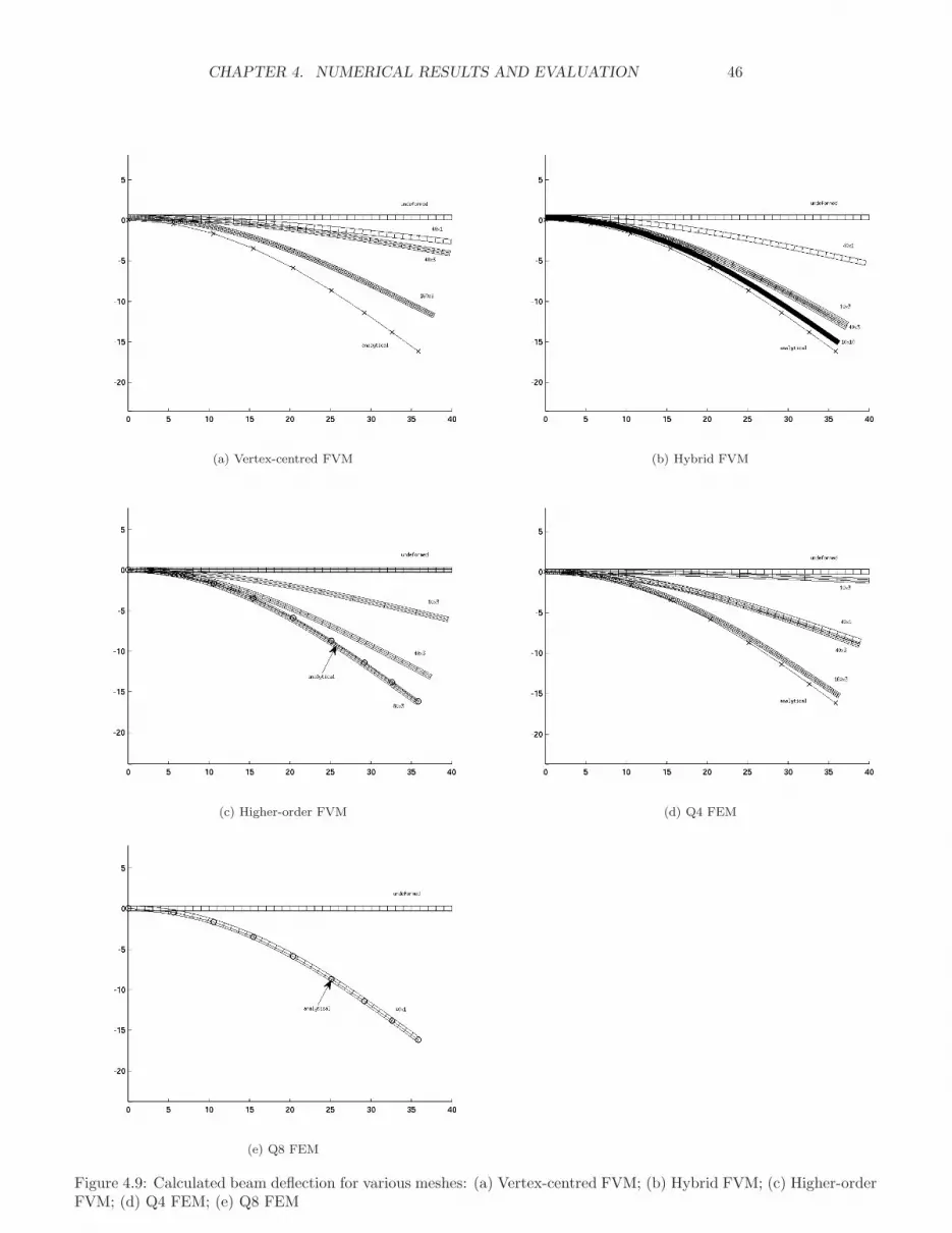
CHAPTER 4. NUMERICAL RESULTS AND EVALUATION 46

(a) Vertex-centred FVM (b) Hybrid FVM

(c) Higher-order FVM (d) Q4 FEM

(e) Q8 FEM

Figure 4.9: Calculated beam deflection for various meshes: (a) Vertex-centred FVM; (b) Hybrid FVM; (c) Higher-orderFVM; (d) Q4 FEM; (e) Q8 FEM

CHAPTER 4. NUMERICAL RESULTS AND EVALUATION 47

Vertex-centred FVM Hybrid FVM

Internal node 0 0Boundary node (top/bottom):

x1-momentum (−1)p+1`

1

3

F

I∆x2 + 1

6

F

I

∆x21

∆x2

´

(−1)p+1`

1

3

F

I∆x2 + 1

6

F

I

∆x21

∆x2

´

+ (−1)p 1

4

F

I

∆x21

∆x2

x2-momentum 0 0Boundary node (right):

x1-momentum 0 0

x2-momentum −1

12

F

I∆x1 + 1

3

F

I

∆x22

∆x1−

1

12

F

I∆x1 + 1

3

F

I

∆x22

∆x1

Corner node (right):x1-momentum 0 0

x2-momentum (−1)p F c

I

∆x2∆x1

(−1)p F c

I

∆x2∆x1

Corner node (left):

x1-momentum (−1)p F L

2I

∆x1∆x2

0

x2-momentum (−1)p F cI

∆x2∆x1

(−1)p F cI

∆x2∆x1

Table 4.2: Errors of vertex-centred and hybrid formulations for a cantilever beam subjected to a tip load

0 10 20 30 40 50 60 70 80 90 1000

0.01

0.02

0.03

0.04

0.05

0.06

Aspect ratio

Dis

plac

emen

t

FVM: VertexFVM: HybridAnalytical

Figure 4.10: Tip displacement as a function of element aspect ratio for a thincantilever beam subjected to a concentrated tip load

CHAPTER 4. NUMERICAL RESULTS AND EVALUATION 48

0 0.2 0.4 0.6 0.8 1 1.2 1.4 1.6 1.8 2−5

−4.5

−4

−3.5

−3

−2.5

−2

−1.5

−1

log(Mesh size)

log(

Err

or)

FVM: HybridFVM: Vertex

2nd order 1st order

Figure 4.11: Convergence rate of displacements

element size in both directions. A plot of the logarithm of the error of tip dis-placements vs. the logarithm of the mesh size is shown in Figure 4.11. Thenegative of the gradient of this curve gives the rate of convergence: 2.0 for thehybrid formulation and 1.9 for the vertex-formulation. Therefore, both formu-lations tend towards second-order accuracy. However, it is clearly evident inFigure 4.11 that for a given mesh spacing the hybrid formulation is more ac-curate than the vertex-centred formulation. These results correlate with thoseobtained from the analytical analysis (Table 3.1): as the meshes get finer, thenumber of internal nodes is significantly more than boundary and corner nodesand the schemes tend towards second-order accuracy.

4.6 Dynamic 2D Beam

The test-cases above assessed the spatial accuracy of the different formulations.It was shown that the Q8 FEM produced the most desirable results. In order toassess temporal accuracy when applied to transient problems, the 2D dynamicbeam test-case (see Figure 4.12) was considered.

The beam has a Young’s modulus E = 0.2 MPa, Poisson’s ratio ν = 0.49,density ρ = 2000 kg m−3, length l = 40 mm and a cross-section of 0.6 mm ×10 mm. One end of the beam was clamped while a shear traction τ = 0.1 Pais suddenly applied at the free end at time t = 0. Analytical solutions whichinclude temporal behaviour are only available for the small displacement case,thus the test-case was subjected to this constraint. A 40×1 Q8 FEM mesh was

CHAPTER 4. NUMERICAL RESULTS AND EVALUATION 49

τ

Figure 4.12: Dynamic beam with applied shear

used in this analysis.The analytical solution in the small displacement limit is a sinusoidal oscil-

lation given by [11]:

u =4τ

E

l3

h2(1 − ν2)

[

1 +3

4(1 + ν)

h2

l2

]

[cos(ω1t) − 1] (4.10)

at a frequency of

ω1 = λ21

√

E

12ρ

h

l2, (4.11)

where λ1 is the eigenvalue of the first mode of oscillation viz. λ1 = 1.875 in thistest-case.

In Figure 4.13(a), the predicted dynamic response of the centre of the beamtip is compared with the analytical solution. The calculated results are plottedevery two timesteps, where the timestep size is 0.005 s. An accurate solutionis obtained with a relatively coarse mesh, the slight difference at the peaks isdue to higher-order modes that are excited in the beam whereas the analyticalsolution only takes into account the first mode of vibration. Using a finer meshand smaller timestep size produces exactly the same results, as shown in Fig-ure 4.13(b), which validates the temporal accuracy of the developed technology.

4.7 Conclusion

The three finite volume methods: vertex-centred FVM, hybrid FVM and higher-order FVM; as well as the two finite element schemes: Q4 FEM and Q8 FEMdeveloped in Chapter 3 were rigorously evaluated on representative test prob-lems of increasing complexity. It was shown that both the vertex-centred FVMand Q4 FEM suffer from shear locking or sensitivity to element aspect ratio.The hybrid FVM is locking-free but many elements are required through thethickness of the structure to obtain accurate results. The higher-order FVMproduced close to exact results for thin structures in bending, when using threeelements through the thickness. However, the Q8 FEM needed only a singleelement through its thickness to produce accurate results for the steady-state

CHAPTER 4. NUMERICAL RESULTS AND EVALUATION 50

0 0.5 1 1.5 2 2.5 3 3.5 4 4.5 5−8

−7

−6

−5

−4

−3

−2

−1

0x 10

−4

t (s)

Tip

dis

plac

emen

t (m

)

AnalyticalQ8: 40 × 1

(a)

0 0.5 1 1.5 2 2.5 3 3.5 4 4.5 5−8

−7

−6

−5

−4

−3

−2

−1

0x 10

−4

t (s)

Tip

dis

plac

emen

t (m

)

∆t = 0.005s

∆t = 0.001sQ8: 80 × 2

(b)

Figure 4.13: Transient response of a cantilever beam when a shear traction of0.1 Pa is suddenly applied at the free end: (a) Q8 40×1 mesh; (b) using differenttimesteps and mesh sizes

CHAPTER 4. NUMERICAL RESULTS AND EVALUATION 51

bending analysis, as well as for the transient analysis. In addition, inherentin the Q8 FEM formulation is the automatic capability of handling problemswith unstructured meshes. Overall, the Q8 FEM is the preferred method formodelling thin geometrically non-linear structures.

Part II

Fluid-Structure Interaction

52

Chapter 5

Fluid-Structure Interaction:

Implementation

5.1 Introduction

In this chapter a hybrid finite volume–finite element fluid-structure interactionformulation is developed by coupling the Q8 finite element formulation for thesolid with the existing finite volume fluid solver within the Elemental frame-work. Many recent FSI efforts have made use of a single discretisation scheme,either finite volume [11, 13, 14, 35] or finite element [1, 10, 36–39], to solve theentire domain, which simplifies the treatment at the interface of the fluid andsolid domain. However, each discretisation method contains certain inherentadvantages and should be used as such. Since the framework within Elementalis independent of discretisation strategy employed, it allows for the develop-ment of a hybrid finite volume–finite element FSI formulation. To the author’sknowledge, this is the first instance in which such a hybrid formulation is ap-plied to strongly-coupled FSI problems. The coupling of a higher-order finiteelement formulation for the structure and a linear finite volume formulation forthe fluid leads to non-matching nodes at the solid interface and the transfer ofinformation at these nodes will also be addressed in this chapter.

The solution of FSI systems range from single or monolithic methods thatare inherently strongly-coupled to separate or partitioned methods that can bestrongly- or weakly-coupled. This work focusses on FSI systems where thereis a strong interaction between the fluid and structural domains and weakly-coupled methods are, therefore, not considered as they may diverge or resultin inaccurate solutions [1, 10, 11]. For strongly-coupled methods, the advantageof a monolithic over a partitioned approach is that all the equations are con-sidered simultaneously and a single system of equations solved, which ensuresstability and convergence. However, this approach may suffer from ill condi-tioning and convergence is generally slow [1]. The advantage of a partitionedapproach is that it allows the use of two independent solution techniques for the

53

CHAPTER 5. FLUID-STRUCTURE INTERACTION: IMPLEMENTATION54

fluid and solid equations in isolation. The drawback of partitioned approachesis that they generally require a separate coupling algorithm or additional outeriterations between the fluid and solid to achieve strong-coupling, which placesan additional computational cost on the scheme [1, 40, 41]. The most popularpartitioned coupling algorithms use fixed-point iteration methods or interfaceNewton-Krylov methods [40, 42]. Fixed-point methods generally make use ofGauss-Seidel iterations which are slow to converge and methods to accelerateconvergence, including Aitken and steepest descent relaxation and coarse-gridpreconditioning, have been used [41–45]. The Newton-Raphson methods requirethe computation of Jacobians, which may be difficult to compute exactly andvarious methods have been developed that use approximate Jacobians [46–48].In this work the fluid and structural domains are to be solved in a strongly-coupled partitioned manner, where the transfer of information occurs at solversub-iteration level negating the need for a separate coupling algorithm. Toensure solver stability and computational speed, a simple interface coupling al-gorithm implemented at sub-iteration level is to be used. Finally, for scalabilityto large problems the scheme is to be implemented in a matrix-free approach andin such a manner that makes it particularly well-suited for distributed memoryparallel hardware architectures.

In this chapter, we introduce the set of governing equations and constitutiverelations that describe the fluid domain. The transfer of information at theinterface of the fluid and solid domains is detailed. Parallelisation of the solveris discussed. Finally, the solution procedure and dynamic mesh movement areexplained.

5.2 Fluid Governing Equation Set

The fluid flow is governed by the Navier-Stokes equations. In general, theseequations are expressed in an Eulerian or spatial frame of reference, as opposedto a Lagrangian or material description for the solid, which entails a fixed spatialregion with fluid flowing through it. For fluid-structure interaction problems thesolid deforms and displaces the fluid domain and a mixture or combination ofthe two reference frames, referred to as an arbitrary-Lagrangian-Eulerian (ALE)reference frame, results for the motion of the FSI interface. This approach wasfirst described by Hirt et al. [63] and later adopted by many others and is nowwidely used for FSI applications [12]. A dynamic mesh movement algorithmthat deforms the fluid mesh is therefore required and is described later.

Assuming a viscous, incompressible and isothermal fluid, the equations gov-erning the fluid flow are given by the continuity and Navier-Stokes equations:

∂vi

∂xi

= 0 (5.1)

ρ∂vi

∂t+ ρ(vj − v∗j )

∂vi

∂xj

+∂p

∂xi

− ∂σij

∂xj

− ρbi = 0 (5.2)

CHAPTER 5. FLUID-STRUCTURE INTERACTION: IMPLEMENTATION55

where ρ, vi, p, σij and bi are the fluid density, fluid velocity, pressure, stressand body forces respectively, xi are the fixed Eulerian coordinates and v∗ is themesh velocity. The term (vj − v∗j ) is an ALE convective velocity that resultsfrom a difference between the fluid velocity and the mesh velocity.

5.3 Fluid Constitutive Equations

To close the governing equations, a constitutive relation for the stress is required.Assuming a Newtonian fluid, the relationship between stress and rate of strainis given by

σij = µ

(

∂vi

∂xj

+∂vj

∂xi

)

, (5.3)

where µ is the fluid viscosity.The equations governing the motion of the fluid, Equations (5.1) to (5.3), are

discretised via a second-order accurate edge-based hybrid-unstructured finitevolume methodology. The incompressibility of the fluid is dealt with usingan artificial-compressibility fractional-step algorithm. The details of this fallbeyond the scope of this work and the reader is referred to [18, 64] for furtherdetails. The coupling between the fluid and solid domain is described in thenext section.

5.4 Fluid-Solid Interface Treatment

The fluid-structure interaction system can be described in general or broadterms as follows: the fluid flow provides a traction or load onto the structure.This results in a dynamic response or deformation of the structure which in turnaffects the geometry of the fluid domain and the fluid flow. In order to solve thisintimately coupled system, the following coupling conditions for the traction,displacement and velocity need to be satisfied at the fluid-solid interface:

tsi = pni − σfijnj (5.4)

ufi = us

i (5.5)

vfi = v∗i = vs

i (5.6)

where ni is the related unit vector pointing outward from the fluid domain andthe superscripts f and s refer to the fluid and solid respectively. Equation (5.4)represents momentum conservation or force equilibrium at the interface, whileEquations (5.5) and (5.6) enforce the kinematic or geometric continuity andno-slip conditions respectively.

5.4.1 Consistent Nodal Loads

In this work the fluid and solid elements coincide at the interface, which simpli-fies the transfer of information between the fluid and solid domains. However,

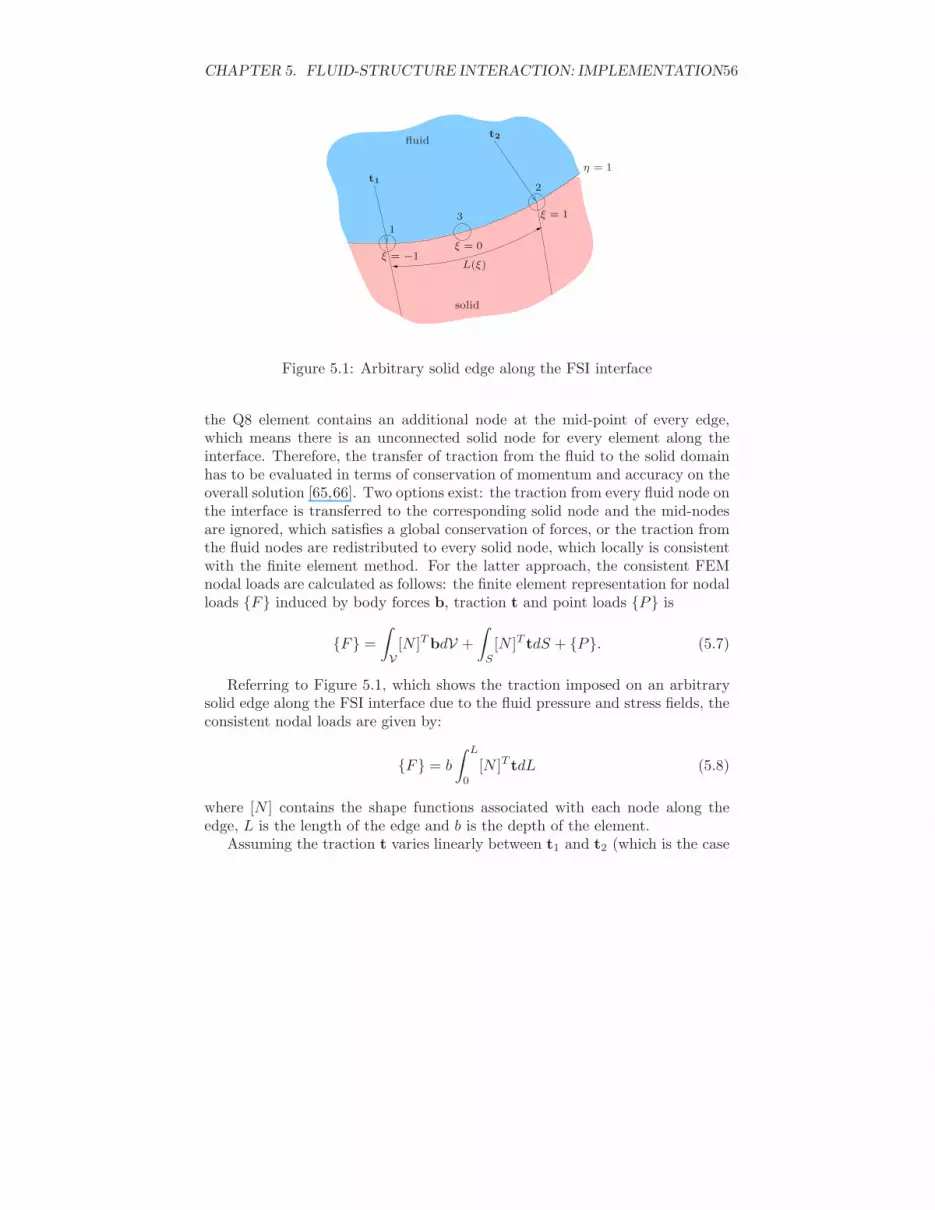
CHAPTER 5. FLUID-STRUCTURE INTERACTION: IMPLEMENTATION56

t1

t2

1

2

3

η = 1

ξ = −1ξ = 0

ξ = 1

L(ξ)

fluid

solid

Figure 5.1: Arbitrary solid edge along the FSI interface

the Q8 element contains an additional node at the mid-point of every edge,which means there is an unconnected solid node for every element along theinterface. Therefore, the transfer of traction from the fluid to the solid domainhas to be evaluated in terms of conservation of momentum and accuracy on theoverall solution [65,66]. Two options exist: the traction from every fluid node onthe interface is transferred to the corresponding solid node and the mid-nodesare ignored, which satisfies a global conservation of forces, or the traction fromthe fluid nodes are redistributed to every solid node, which locally is consistentwith the finite element method. For the latter approach, the consistent FEMnodal loads are calculated as follows: the finite element representation for nodalloads {F} induced by body forces b, traction t and point loads {P} is

{F} =

∫

V

[N ]T bdV +

∫

S

[N ]T tdS + {P}. (5.7)

Referring to Figure 5.1, which shows the traction imposed on an arbitrarysolid edge along the FSI interface due to the fluid pressure and stress fields, theconsistent nodal loads are given by:

{F} = b

∫ L

0

[N ]T tdL (5.8)

where [N ] contains the shape functions associated with each node along theedge, L is the length of the edge and b is the depth of the element.

Assuming the traction t varies linearly between t1 and t2 (which is the case

CHAPTER 5. FLUID-STRUCTURE INTERACTION: IMPLEMENTATION57

with the fluid discretisation [34]), Equation (5.8) can be expanded as

F1x1

F1x2

F2x1

F2x2

F3x1

F3x2

= b

∫ 1

−1

N1 00 N1

N2 00 N2

N3 00 N3

[

S1

{

t1x1

t1x2

}

+ S2

{

t2x1

t2x2

}]

dL

dξdξ, (5.9)

where the integral is transformed to the natural coordinate system and Si arethe linear shape functions assumed for the traction, i.e.

S1 = 12 (1 − ξ) S2 = 1

2 (1 + ξ) . (5.10)

Since the solid elements are Q8 elements, the quadratic shape functionsassociated with each node along the edge are

N1 = − 12ξ(1 − ξ) N2 = 1

2ξ(1 + ξ) N3 = (1 − ξ2) . (5.11)

Assuming straight edges in the undeformed configuration, which is valid forproblems considered in this work, the length of the edge can be expressed in thenatural coordinate system as

L(ξ) = N1L1 + N2L2 + N3L3, (5.12)

therefore the derivative of L with respect to ξ, used in Equation (5.9), is

dL

dξ=

dN1

dξL1 +

dN2

dξL2 +

dN3

dξL3 (5.13)

= −1

2(1 − 2ξ)L1 +

1

2(1 + 2ξ)L2 − 2ξL3. (5.14)

Substituting Equations (5.10) to (5.14) into Equation (5.9) gives

F1x1

F1x2

F2x1

F2x2

F3x1

F3x2

= b

∫ 1

−1

− 12ξ(1 − ξ) 0

0 − 12ξ(1 − ξ)

12ξ(1 + ξ) 0

0 12ξ(1 + ξ)

(1 − ξ2) 00 (1 − ξ2)

{

12 (1 − ξ)t1x1

+ 12 (1 + ξ)t2x1

12 (1 − ξ)t1x2

+ 12 (1 + ξ)t2x2

}(

−1

2(1 − 2ξ)L1 +

1

2(1 + 2ξ)L2 − 2ξL3

)

dξ.

(5.15)

The integrand is a fourth-order polynomial. Analytical integration gives the

CHAPTER 5. FLUID-STRUCTURE INTERACTION: IMPLEMENTATION58

closed form expressions:

F1x1

F1x2

F2x1

F2x2

F3x1

F3x2

=

− b30 (13L1t1x1

+ 2L1t2x1+ 3L2t1x1

+ 2L2t2x1− 16L3t1x1

− 4L3t2x1)

− b30 (13L1t1x2

+ 2L1t2x2+ 3L2t1x2

+ 2L2t2x2− 16L3t1x2

− 4L3t2x2)

b30 (2L1t1x1

+ 3L1t2x1+ 2L2t1x1

+ 13L2t2x1− 4L3t1x1

− 16L3t2x1)

b30 (2L1t1x2

+ 3L1t2x2+ 2L2t1x2

+ 13L2t2x2− 4L3t1x2

− 16L3t2x2)

− b15 (7L1t1x1

+ 3L1t2x1− 3L2t1x1

− 7L2t2x1− 4L3t1x1

+ 4L3t2x1)

− b15 (7L1t1x2

+ 3L1t2x2− 3L2t1x2

− 7L2t2x2− 4L3t1x2

+ 4L3t2x2)

.

(5.16)

The expressions above give the consistent FEM nodal loads for each nodealong the FSI interface as a function of the tractions imposed by the fluiddomain.

5.4.2 FSI Interface Coupling Scheme

It is known that partitioned FSI system solvers may be unstable for certainstrongly-coupled problems [12]. The 1D piston-channel problem described in thenext chapter constitutes a good example of such a case [1,12]. To ensure stabilitywithout any additional computational overhead, a new interface coupling schemeis therefore proposed. The scheme is based on the fact that within each iterationin pseudo-time, the fluid passes forces to the solid which causes it to displace ordeform based on the solid governing equations and without any considerationof the fluid domain. If the forces are large or the density of the solid low, thismay render the system unstable. If instead the forces from the fluid domainare projected forward based on the inertia of the fluid, the solid will deformaccordingly and the fluid-solid system remains stable. The projection of thefluid force in pseudo-time is stated mathematically as

F τ+∆τi = F τ

i +dF

da

∣

∣

∣

∣

τ

i

∆ai, (5.17)

where Fi is the applied force on any arbitrary solid node along the FSI interfaceand ai is the acceleration. Note that since the solution is driven to pseudo-steadystate, F τ+∆τ

i = F τi upon convergence and the projected term is nullified.

The term dFda

represents the inertia of the fluid and can be approximatednumerically as

dF

da

∣

∣

∣

∣

τ

i

≈ F τ−∆τi − F τ−2∆τ

i

aτ−∆τi − aτ−2∆τ

i

. (5.18)

Substituting Equation (5.18) into Equation (5.17) and expanding gives:

F τ+∆τi ≈ F τ

i +F τ−∆τ

i − F τ−2∆τi

aτ−∆τi − aτ−2∆τ

i

(aτ+∆τi − aτ

i ) (5.19)

≈ F τi +

F τ−∆τi − F τ−2∆τ

i

aτ−∆τi − aτ−2∆τ

i

(

vτ+∆τi − vn

i

∆t− vτ

i − vni

∆t

)

(5.20)

CHAPTER 5. FLUID-STRUCTURE INTERACTION: IMPLEMENTATION59

where vi is the velocity of the node in the i-direction.The velocity vτ+∆τ

i in Equation (5.20) is the value being solved for in thecurrent pseudo-timestep. Therefore, following from Equation (3.88):

∑

e

[Me]Q8lumped

{vi}τ+∆τ − {vi}τ

∆τ≈ {Fi}τ+∆τ−

∑

e

(

∑

Gauss pts

[B]T {P}det(J)WGP

)

−∑

e

[Me]Q8cons

3{vi}τ+∆τ − 4{vi}n + {vi}n−1

2∆t. (5.21)

Now, substituting Equation (5.20) for the force gives:

∑

e

[Me]Q8lumped

{vi}τ+∆τ − {vi}τ

∆τ≈ {Fi}τ+

{Fi}τ−∆τ − {Fi}τ−2∆τ

{ai}τ−∆τ − {ai}τ−2∆τ

({vi}τ+∆τ − {vi}τ

∆t

)

−∑

e

(

∑

Gauss pts

[B]T {P}det(J)WGP

)

−∑

e

[Me]Q8cons

3{vi}τ+∆τ − 4{vi}n + {vi}n−1

2∆t,

(5.22)

where {•} indicates a vector containing components of that variable within anelement.

Equation (5.22) is re-arranged to solve for the velocity vτ+∆τi in an ex-

plicit fashion. This proposed interface coupling scheme requires little additionalcomputational overhead, and is evaluated on the 1D piston-channel system inChapter 6.

5.5 Parallelisation

The edge-based matrix-free numerical method lends itself easily to the use ofdistributed memory parallel hardware architectures. For this purpose, the meshis decomposed into a number of subdomains for parallel operation. Since thesolution procedure is an edge-based one, the number of edges in each subdo-main is of a similar magnitude. The METIS library [67] is used for domaindecomposition. One layer of overlapping or ghost nodes is needed for trans-ferring information between subdomains. For edges that lie on the boundariesof the subdomains, the ghost nodes are treated as slave nodes, the values onwhich are updated from their corresponding master nodes in the neighbouringdomain. Message Passing Interface (MPI) is used to communicate data betweendomains.

5.6 Mesh Movement and Solution Procedure

The movement of the fluid mesh is handled via an interpolation procedure. Inthis approach the closest internal and external boundary nodes for every internalfluid node are identified and the distances between the boundary nodes and the

CHAPTER 5. FLUID-STRUCTURE INTERACTION: IMPLEMENTATION60

internal node computed at the beginning of the analysis. The movement ofinternal fluid nodes is then determined by means of an interpolation functionthat uses the displacements of the closest boundary nodes. The reader is referredto [17] for further details.

The solution procedure for the coupled FSI problem involves solving thediscretised fluid and solid governing equations and updating the mesh in aniterative manner that effects strong coupling, as follows:

1. The fluid governing equations, Equations (5.1) to (5.3), are solved for aniteration. This solution provides tractions that are applied to the soliddomain.

2. The solid discrete equations, Equations (3.84) and (3.92), are then solvedfor an iteration, which provides velocities and displacements at the bound-ary of the FSI interface. The boundary velocities are applied to the fluidmesh, which results in an ALE convective velocity in the fluid domain.

3. The mesh is moved if the displacement of a solid mesh boundary nodeexceeds 30% of the element size or the residuals of the fluid and soliddiscrete equations have decreased by at least four orders of magnitude.

4. The steps above are repeated until convergence, i.e. the residuals of fluidand solid discrete equations are calculated and if greater than the conver-gence tolerance, Steps 1 to 3 are repeated. If the residuals have decreasedby at least five orders of magnitude, the real-timestep is terminated andthe next timestep is entered by proceeding to Step 1.

5.7 Conclusion

In this chapter, a partitioned hybrid finite volume–finite element fluid-structureinteraction scheme for strongly-coupled problems was developed. The governingequation set and constitutive relations that describe a viscous, incompressiblefluid were presented. The transfer of information between the fluid and soliddomains, including the coupling of the Q8 solid elements with the finite vol-ume fluid elements, was described in detail. Parallelisation of the solver wasexplained. Finally, mesh movement and a solution procedure that effects strongcoupling between the fluid and solid domains were detailed.

Chapter 6

Fluid-Structure Interaction:

Validation and Verification

6.1 Introduction

In this chapter, the developed FSI technology is evaluated on three strongly-coupled benchmark problems. In the first example, a 1D piston-channel systemwith a varying fluid domain is studied. The second example considers an elasticbeam in the wake of a square block undergoing vortex-induced vibration in itssecond mode. Finally, the same block-tail geometry as the previous case butwith the beam oscillating in its first mode of vibration is analysed. Solutionsare considered converged if the residuals decrease by at least five orders ofmagnitude. Results are compared with those published in literature as well asanalytical solutions where available.

6.2 Dynamic Piston-channel System

The first test-case considered was that of a piston-channel system with a vary-ing fluid domain. The system geometry and boundary conditions are describedin Figure 6.1. The channel is 11 m long and is partially filled with an inviscidincompressible fluid with an elastic piston situated to its left. A prescribed ve-locity, v(t), was imposed on the piston, which pushes the fluid out of the domain.A zero pressure boundary condition was imposed at the outflow boundary andslip boundary conditions were imposed along all the channel walls. The pis-ton has a Young’s modulus of E = 10 Pa and density and Poisson’s ratio ofzero. A linear elastic solid model was used for this problem for comparison withothers [1]. The fluid has a density ρf = 1 kg m−3.

This problem was chosen as the coupling between the fluid and solid domainis strong and partitioned FSI solution schemes usually diverge for such a prob-lem, even with large under-relaxation [1, 12]. This would test the partitioned

61

CHAPTER 6. FLUID-STRUCTURE INTERACTION: VALIDATION AND VERIFICATION62

1 m

1 m

10 m

p = 0

slip

slip

solid fluid

v(t) = 0.2t

Figure 6.1: Geometry and boundary conditions for the piston-channel system

k

m(t)

int

v(t) = 0.2t

Figure 6.2: Representative spring-mass system for the piston-channel configu-ration

FSI interface coupling scheme proposed in the previous chapter. An analyticalsolution exists for this system, which can be considered as a simple 1D problem.

To obtain an analytical expression for the displacement and velocity of theinterface, the system can be treated as a 1D spring-mass system, as shown inFigure 6.2. The elastic piston acts as a linear spring and the incompressiblefluid as a variable mass [1]. Applying a balance of forces at the interface gives:

Fspring + Fmass = 0 (6.1)

therefore,

k(uint − u(t)) = −mdvint

dt(6.2)

where Fspring and Fmass are the forces exerted by the spring and mass, uint andvint are the displacement and velocity of the interface, u(t) is the prescribeddisplacement of the left wall, k is the equivalent spring constant and m is themass of the fluid. Substituting the properties of the piston and fluid for thespring and mass respectively, yield the following expressions for the velocityand displacement at the interface of the sytem:

dvint

dt=

10(uint − 0.1t2)

(uint − 10)(6.3)

duint

dt= vint. (6.4)

CHAPTER 6. FLUID-STRUCTURE INTERACTION: VALIDATION AND VERIFICATION63

The solid domain is discretised using a single Q8 element and the fluid do-main using three cells. The resulting computed time history of the displacementand velocity of the interface are shown in Figure 6.3. As can be seen, the FSIscheme was able to predict the exact solution. Figure 6.4 shows the resultsobtained using different meshes for the fluid and solid domain, i.e. one solid andten fluid cells (1 × 10), one solid and twenty fluid cells (1 × 20), and five solidand ten fluid cells (5 × 10). This demonstrates stability and robustness in thescheme.

0 1 2 3 4 5 6 7 8 9 100

1

2

3

4

5

6

7

8

9

10

t (s)

Dis

plac

emen

t (m

)

ResultsAnalytical

Figure 6.3: Displacement (left) and velocity (right) of the interface of the piston and channel

0 1 2 3 4 5 6 7 8 9 100

1

2

3

4

5

6

7

8

9

10

t (s)

Dis

plac

emen

t (m

)

Mesh: 1x10Mesh: 1x20Mesh: 5x10

0 1 2 3 4 5 6 7 8 9 100

0.5

1

1.5

2

2.5

t (s)

Vel

ocity

(m

/s)

Mesh: 1x10Mesh: 1x20Mesh: 5x10

Figure 6.4: Displacement (left) and velocity (right) of the interface of the piston-channel usingvarious meshes

CHAPTER 6. FLUID-STRUCTURE INTERACTION: VALIDATION AND VERIFICATION64

Figure 6.5: Velocity contours of the piston and pressure contours of the fluid at various times

Velocity contours of the solid and pressure contours of the fluid at varioustimes are shown in Figure 6.5. The velocity field is linear in the solid, while thepressure field is linear in the fluid. A second-order accurate scheme is thus ableto predict the solution exactly.

6.3 Block-tail in Second Mode of Vibration

The second test-case considered was that of an elastic beam in the wake of arigid square block. This is a popular FSI benchmark test-case that was firstproposed by Wall [68] and studied by many other researchers [1,10,14,39]. Thegeometry and boundary conditions are shown in Figure 6.6. The properties ofthe incompressible fluid are: density ρf = 1.18 × 10−3 g cm−3 and viscosityµf = 1.82 × 10−4 g cm−1 s−1, while that of the beam are: density ρs = 2.0 gcm−3, Young’s modulus E = 2.0×106 g cm−1 s−2 and Poisson’s ratio ν = 0.35.The plane stress assumption was used. A uniform constant fluid velocity, vin =31.5 cm s−1, or Reynolds number, Re =

ρf Lvin

µf= 204, was applied at the inlet

while at the exit the pressure was set to zero. The artificial projection term, asdescribed in the previous chapter, was not necessary for this problem.

The fluid domain was discretised into an unstructured triangular mesh con-sisting of approximately 6 000 elements as shown in Figures 6.7(a) and 6.7(b).The solid was discretised using a single layer of 40 Q8 elements. Plots of thedeformed mesh that results from the oscillations of the beam are shown in Fig-ures 6.7(c) and 6.7(d).

CHAPTER 6. FLUID-STRUCTURE INTERACTION: VALIDATION AND VERIFICATION65

Slip boundary condition

Slip boundary condition

pout = 0vin = 31.5 cm s−1

4 cm4.5 cm

1 cm

1 cm

0.06 cm

10 cm

12 cm

Figure 6.6: Geometry and boundary conditions for the block-tail FSI test-case

(a) (b)

(c) (d)

Figure 6.7: Block-tail test-case: (a) and (b) 6 000 element fluid mesh. (c) and (d) Plots of the deformedmesh

CHAPTER 6. FLUID-STRUCTURE INTERACTION: VALIDATION AND VERIFICATION66

The inlet velocity results in vortices that are shed from the corners of theblock periodically at a frequency of 3.7 Hz, which is close to the second naturalfrequency of the beam of 3.8 Hz. The fluid passes over the beam as symmetricvortices develop on either side of it. The symmetry of the vortices breaks, whichresults in uneven forces on the beam inducing vibrations of small amplitude.The oscillation of the beam results in further disturbance of the flow, which inturn induces larger displacements of the beam. Within each period, two vorticesdevelop on one side of the beam while a larger vortex develops on the other side,as shown in Figure 6.8. The system builds up to large oscillations of the beamin its second mode of vibration as vortices are shed periodically from either sideof it.

The time history of the tip displacement of the beam is plotted in Fig-ure 6.9(a), together with the results of Hubner et al. [1]. There is a good

Figure 6.8: Pressure (left) and velocity contours (right) for the block-tail test-case with the beam oscillatingin its second mode of vibration

CHAPTER 6. FLUID-STRUCTURE INTERACTION: VALIDATION AND VERIFICATION67

correlation between the two sets of results, with the amplitude and frequencydiffering by less than 3% and 4% respectively as shown in Table 6.1. A rigor-ous mesh and temporal independence study was conducted. To evaluate meshindependence of the fluid two finer meshes of 25 000 and 50 000 fluid elementswere generated (shown in Figure 6.10). As can be seen in Figure 6.9(b) andTable 6.1, a small change in solution is observed from the 6 000 to the 25 000element mesh, but a further doubling of the number of elements results in anegligible difference. Next, to evaluate mesh independence of the solid a finersolid mesh of 80 × 2 Q8 elements was used and it was found that the resultsare identical to the 40 × 1 solid mesh case (see Figure 6.9(c) and Table 6.1).Finally, temporal independence was evaluated by using four different timestepsizes varying from 0.005s to 0.0005s. The time history in Figure 6.9(d) as well asthe result in Table 6.1 show good convergence and independence in the results.

An evaluation of the transfer of traction forces from the fluid to the solid do-main was conducted. The fluid and solid elements line up at the fluid-structureinterface. However, since the Q8 element contains an additional node at themid-point of every edge there is an additional unconnected solid node at theFSI interface. This complicates the transfer of the traction forces: either thetraction at every fluid node on the interface is transferred to the correspondingsolid node, which will satisfy a global balance of force, or FEM nodal loads,as described in the previous chapter and which are consistent with the finiteelement method, are calculated and the traction distributed to every solid nodeat the interface. Both approaches were implemented and a comparison of thetip displacement is shown in Figure 6.11. There is a negligible change in resultand for practical purposes a simple transfer of traction from every fluid node tothe corresponding solid node on the interface is sufficient, if structural stresseson the interface are not of primary concern.

Fluid mesh Solid mesh Timestep (s) Amplitude (cm) Frequency (Hz)

6 000 40 × 1 0.001 0.78 2.986 000 80 × 2 0.001 0.78 2.9825 000 120 × 1 0.001 0.76 2.9750 000 160 × 1 0.001 0.76 2.976 000 40 × 1 0.0005 0.78 2.97

Hubner et al. [1] 0.8 3.1

Xia et al. [14] 0.81 3.3

Table 6.1: Comparison of amplitude and frequency for the block-tail test-casein second mode of vibration with various meshes and timestep sizes

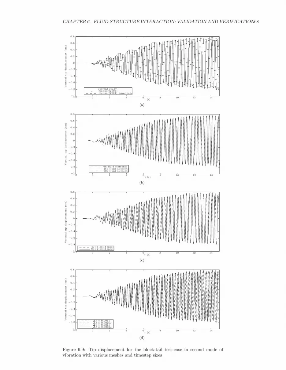
CHAPTER 6. FLUID-STRUCTURE INTERACTION: VALIDATION AND VERIFICATION68

current studyHubner(2004)Hubner(2004) amplitude

Vertic

altip

dis

pla

cem

ent

(cm

)

t (s)−2 2 4 6 8 10 12 14

−1

−0.8

−0.6

−0.4

−0.2

0

0

0.2

0.4

0.6

0.8

(a)

6k fluid elements25k fluid elements50k fluid elements

Vertic

altip

dis

pla

cem

ent

(cm

)

t (s)−2 2 4 6 8 10 12 14

−1

−0.8

−0.6

−0.4

−0.2

0

0

0.2

0.4

0.6

0.8

(b)

40×1 solid mesh80×2 solid mesh

Vertic

altip

dis

pla

cem

ent

(cm

)

t (s)−2 2 4 6 8 10 12 14

−1

−0.8

−0.6

−0.4

−0.2

0

0

0.2

0.4

0.6

0.8

(c)

∆t = 0.005s∆t = 0.0025s∆t = 0.001s∆t = 0.0005s

Vertic

altip

dis

pla

cem

ent

(cm

)

t (s)−2 2 4 6 8 10 12 14

−1

−0.8

−0.6

−0.4

−0.2

0

0

0.2

0.4

0.6

0.8

(d)

Figure 6.9: Tip displacement for the block-tail test-case in second mode ofvibration with various meshes and timestep sizes

CHAPTER 6. FLUID-STRUCTURE INTERACTION: VALIDATION AND VERIFICATION69

Figure 6.10: Block-tail test-case: 25 000 (left) and 50 000 cell (right) fluid mesh

force: lumpedforce: consistent

Vertic

altip

dis

pla

cem

ent

(cm

)

t (s)−2 2 4 6 8 10 12

−1

−0.8

−0.6

−0.4

−0.2

0

0

0.2

0.4

0.6

0.8

Figure 6.11: Tip displacement for the block-tail test-case in second mode ofvibration using consistent and lumped traction forces at the interface

CHAPTER 6. FLUID-STRUCTURE INTERACTION: VALIDATION AND VERIFICATION70

6.4 Block-tail in First Mode of Vibration

In the final test-case, the same block-tail geometry as above was consideredbut the beam was given an initial deflection due to a temporary load and theplane strain assumption was used. This problem was considered by Hubner etal. [1]. In order to fit the initial deflection of the beam as shown in [1], thepiecewise-constant tip-load as a function of time was determined empiricallyand is shown in Table 6.2. The behaviour of the system changes significantlyas large-amplitude oscillations of the beam occur in its first mode of vibration.The amplitude is more than twice that of the previous example and plots of thedeformed mesh are shown in Figure 6.12.

The large deflection of the beam causes a vortex to develop on the oppositeside of the deflection. This vortex moves along the beam and breaks away as thebeam reaches its maximum deflection. As the beam moves in the other direction,a smaller vortex of opposite rotation develops at its tip and also breaks away.Plots of the pressure and velocity contours are shown in Figure 6.13.

The tip displacement of the beam is compared with the results of Hubneret al. [1] in Figure 6.14(a). There is a difference in the initial response, butthe results compare well as the limit-cycle is reached. A comparison of theresults using three fluid meshes of 6 000, 25 000 and 50 000 elements is shownin Figure 6.14(b). There is a significant change in the solution from the 6 000to the 25 000 element mesh, but negligible change between the 25 000 and 50000 element mesh. A refinement in the solid mesh has no effect on the result,as shown in Figure 6.14(c). An evaluation of the results using four differenttimestep sizes again shows good temporal independence of the solution (seeFigure 6.14(d)). A comparison of the frequency and amplitude for differentmeshes and timestep sizes is shown in Table 6.3.

Time (s): 0–0.1 0.1–0.15 0.15–0.2 0.2–0.3 0.3–0.4 0.4–0.5 0.5–0.6Force (g cm s−2): 0 0.35 1.5 2.3 3.1 4.2 6.5Time (s): 0.6–0.7 0.7–0.8 0.8–0.9 0.9–1.0 1.0–1.1 1.1–1.2 1.2–1.3Force (g cm s−2): 6.5 5.5 5.0 4.0 3.0 2.0 1.0

Table 6.2: Piecewise-constant force as a function of time applied to tip of beamto reproduce initial deflection in results of [1].

CHAPTER 6. FLUID-STRUCTURE INTERACTION: VALIDATION AND VERIFICATION71

Figure 6.12: Block-tail test-case: Plots of the deformed mesh with the beam oscillating in its first mode ofvibration

Figure 6.13: Pressure (left) and velocity contours (right) for the block-tail test-case with the beam oscil-lating in its first mode of vibration

CHAPTER 6. FLUID-STRUCTURE INTERACTION: VALIDATION AND VERIFICATION72

0 5 10 15−2.5

−2

−1.5

−1

−0.5

0

0.5

1

1.5

2

2.5

t (s)

Ver

tical

tip

disp

lace

men

t (cm

)

current studyHubner(2004)

(a)

0 2 4 6 8 10 12 14 16 18 20−2.5

−2

−1.5

−1

−0.5

0

0.5

1

1.5

2

2.5

t (s)

Ver

tical

tip

disp

lace

men

t (cm

)

6k fluid elements25k fluid elements50k fluid elements

(b)

0 2 4 6 8 10 12 14 16 18 20−2.5

−2

−1.5

−1

−0.5

0

0.5

1

1.5

2

2.5

t (s)

Ver

tical

tip

disp

lace

men

t (cm

)

40x1 solid mesh80x2 solid mesh

(c)

0 2 4 6 8 10 12 14 16 18 20−2.5

−2

−1.5

−1

−0.5

0

0.5

1

1.5

2

2.5

t (s)

Ver

tical

tip

disp

lace

men

t (cm

)

∆t=0.005s

∆t=0.0025s

∆t=0.001s

∆t=0.0005s

(d)

Figure 6.14: Tip displacement for the block-tail test-case in first mode of vibration with various meshes and timestepsizes

CHAPTER 6. FLUID-STRUCTURE INTERACTION: VALIDATION AND VERIFICATION73

Fluid mesh Solid mesh Timestep (s) Amplitude (cm) Frequency (Hz)

6 000 40 × 1 0.001 2.04 0.846 000 80 × 2 0.001 2.04 0.8425 000 120 × 1 0.001 2.17 0.8350 000 160 × 1 0.001 2.18 0.826 000 40 × 1 0.0005 2.04 0.84

Hubner et al. [1] 2.0 0.8

Table 6.3: Comparison of amplitude and frequency for the block-tail test-casein first mode of vibration with various meshes and timestep sizes

6.5 Conclusion

The hybrid finite volume-finite element FSI scheme was tested on three strongly-coupled benchmark FSI test-cases. In all cases the scheme produced accurateresults that compared well with that published in literature. Temporal andmesh independence were evaluated and demonstrated stability and robustnessin the scheme.

Chapter 7

Conclusions and Future

Work

7.1 Consolidation of Work Performed

The aim of this project was to develop an in-house computational tool that canaccurately model strongly-coupled fluid-structure interaction problems, with aparticular focus on thin-walled structures undergoing large, non-linear deforma-tions.

The first objective was to improve the efficiency with which Elemental mod-els thin structures in bending. The finite element method of discretisation istraditionally more common for computational solid mechanics, but the finitevolume method is receiving increased attention for this purpose and both meth-ods were evaluated for this purpose. With regards to the former, linear Q4and higher-order Q8 finite element methods were implemented. For the latter,a standard vertex-centred and recently developed hybrid finite volume methodwere implemented. An in-depth error analysis was conducted on these two for-mulations from which a new higher-order finite volume method was developed.The accuracy of each formulation was compared via application to a number oftest problems. It was shown that both the vertex-centred finite volume methodand Q4 finite element method suffer from shear locking or sensitivity to elementaspect ratio. The structure becomes stiffer as the aspect ratio is increased. Theshear locking mechanism is overcome by the hybrid approach, but many ele-ments are required through the thickness to ensure accuracy. The higher-orderfinite volume method provided accurate results with relatively coarse meshes,but the Q8 finite element method produced the most desirable results and waschosen as the preferred method for modelling the structural domain.

In the second part of this work, a partitioned hybrid finite volume–finiteelement fluid-structure interaction scheme for strongly-coupled problems wasdeveloped. The physical domain consisted of a homogeneous isotropic elasticsolid region and a viscous incompressible isothermal fluid domain, the former

74

CHAPTER 7. CONCLUSIONS AND FUTURE WORK 75

discretised using an isoparametric Q8 finite element methodology and the latterusing an edge-based hybrid-unstructured vertex-centred finite volume method-ology. A dual-timestepping procedure was employed in a way that both thefluid and structural domain are fully or strongly-coupled at solver sub-iterationlevel. The transfer of information between the fluid and solid domains, includ-ing the coupling of the Q8 solid elements with the finite volume fluid elementsand a fluid-solid interface coupling algorithm, was described in detail. Thesolver was parallelised for distributed memory parallel hardware architecturesand movement of the fluid mesh was handled via an interpolation procedure.The developed hybrid finite volume-finite element FSI scheme was validated suc-cessfully on three strongly-coupled benchmark FSI test-cases. In all cases thescheme produced accurate results that compared well with that published inliterature. Temporal and mesh independence were evaluated and demonstratedstability and robustness in the scheme.

7.2 Future Work

The scope of this study was limited to isotropic elastic structures and incom-pressible flows and applied to two-dimensional problems. Further work, buildingon this, is required to furnish a comprehensive industrial fluid-structure inter-action code. Aspects meriting further investigation include:

• The application to 3D problems, which requires the extension of both thefluid and structural solver to a third spatial dimension.

• A stability analysis on the higher-order finite volume method and theestablishment of higher-order finite volume techniques.

• An investigation into the use of shell theory for modelling the structuraldomain and its applicability to a certain class of problems.

• The extension of the fluid-structure interaction solver for a broader rangeof problems. This could include incorporating triangular and mixed finiteelements to handle incompressibility or material non-linearity such as inbiomedical applications. In addition, an extension of the fluid solver tohandle transonic and compressible flows would extend its capability tocapture shocks and increase its use in aerospace applications.

Appendix A

Error Analysis: Analytical

Approach

In order to develop a higher-order finite volume formulation, a detailed erroranalysis was conducted analytically on both the vertex-centred and hybrid for-mulations. The detailed derivations are shown in this section.

To simplify the mathematical analysis yet still obtain a qualitative descrip-tion of the error terms, the problem was limited to the small displacement caseand a Poisson’s ratio of zero was assumed. The governing equation is given byEquation (3.55):

∂σij

∂xj

= 0. (A.1)

The stress-strain relationship is given by Equation (3.57):

σij = Eεij . (A.2)

The strain-displacement relationship for the small displacement case is:

εij =1

2

(

∂ui

∂xj

+∂uj

∂xi

)

. (A.3)

Substituting Equation (A.2) and Equation (A.3) into Equation (A.1) givesthe governing equation expressed in terms of displacements:

E

2

(

∂2ui

∂x2j

+∂2uj

∂xi∂xj

)

= 0. (A.4)

The analytical expressions for the x1- and x2-momentum equations are there-fore, respectively:

∂σ11

∂x1+

∂σ12

∂x2= E

∂2u1

∂x21

+E

2

(

∂2u1

∂x22

+∂2u2

∂x1∂x2

)

= 0 (A.5)

76

APPENDIX A. ERROR ANALYSIS: ANALYTICAL APPROACH 77

∂σ21

∂x1+

∂σ22

∂x2= E

∂2u2

∂x22

+E

2

(

∂2u2

∂x21

+∂2u1

∂x1∂x2

)

= 0 (A.6)

where the nomenclature is as previously defined.We now develop the discrete expressions for the x1- and x2-momentum equa-

tions and expand each using Taylor series expansions. By comparing the an-alytical and expanded discrete expressions, the leading-order error terms areobtained. The discrete expressions differ for an internal, boundary and cornernode and each case is considered separately below.

Internal Node - Vertex-centred FVM

Considering first the vertex-centred finite volume formulation for an internalnode, Figure A.1.

(x1, x2)

∆x1

∆x2

Figure A.1: Schematic of the mesh indicating an internal node

The partial derivatives of stress in the momentum equations, Equations (A.5)and (A.6), are computed as follows:

∂σ11

∂x1≈ σ11(x1 + 1

2∆x1, x2) − σ11(x1 − 12∆x1, x2)

∆x1(A.7)

∂σ12

∂x2≈ σ12(x1, x2 + 1

2∆x2) − σ12(x1, x2 − 12∆x2)

∆x2(A.8)

∂σ21

∂x1≈ σ21(x1 + 1

2∆x1, x2) − σ21(x1 − 12∆x1, x2)

∆x1(A.9)

∂σ22

∂x2≈ σ22(x1, x2 + 1

2∆x2) − σ22(x1, x2 − 12∆x2)

∆x2. (A.10)

Using the stress-strain relation, Equation (A.2), and the strain-displacementrelationship, Equation (A.3), the stress terms are given by:

σ11

(

x1 +1

2∆x1, x2

)

= E∂u1

∂x1

∣

∣

∣

∣

(x1+12 ∆x1,x2)

(A.11)

APPENDIX A. ERROR ANALYSIS: ANALYTICAL APPROACH 78

σ22

(

x1, x2 +1

2∆x2

)

= E∂u2

∂x2

∣

∣

∣

∣

(x1,x2+12∆x2)

(A.12)

σ12

(

x1, x2 +1

2∆x2

)

=E

2

(

∂u1

∂x2+

∂u2

∂x1

)∣

∣

∣

∣

(x1,x2+12∆x2)

(A.13)

σ21

(

x1 +1

2∆x1, x2

)

=E

2

(

∂u2

∂x1+

∂u1

∂x2

)∣

∣

∣

∣

(x1+12∆x1,x2)

. (A.14)

Finally, the displacement gradients for the vertex-centred finite volume for-mulation are computed from Equation (3.50) as:

∂u1

∂x1

∣

∣

∣

∣

(x1+12∆x1,x2)

≈ u1(x1 + ∆x1, x2) − u1(x1, x2)

∆x1(A.15)

∂u2

∂x2

∣

∣

∣

∣

(x1,x2+12∆x2)

≈ u2(x1, x2 + ∆x2) − u2(x1, x2)

∆x2(A.16)

∂u1

∂x2

∣

∣

∣

∣

(x1,x2+12∆x2)

≈ u1(x1, x2 + ∆x2) − u1(x1, x2)

∆x2(A.17)

∂u2

∂x1

∣

∣

∣

∣

(x1,x2+12∆x2)

≈ 1

2

(

∂u2

∂x1

∣

∣

∣

∣

(x1,x2+∆x2)

+∂u2

∂x1

∣

∣

∣

∣

(x1,x2)

)

≈ 1

4∆x1

[

u2(x1 + ∆x1, x2 + ∆x2) + u2(x1 + ∆x1, x2)

− u2(x1 − ∆x1, x2 + ∆x2) − u2(x1 − ∆x1, x2)

]

(A.18)

∂u1

∂x2

∣

∣

∣

∣

(x1+12∆x1,x2)

≈ 1

2

(

∂u1

∂x2

∣

∣

∣

∣

(x1+∆x1,x2)

+∂u1

∂x2

∣

∣

∣

∣

(x1,x2)

)

≈ 1

4∆x2

[

u1(x1 + ∆x1, x2 + ∆x2) + u1(x1, x2 + ∆x2)

− u1(x1 + ∆x1, x2 − ∆x2) − u1(x1, x2 − ∆x2)

]

(A.19)

∂u2

∂x1

∣

∣

∣

∣

(x1+12∆x1,x2)

≈ u2(x1 + ∆x1, x2) − u2(x1, x2)

∆x1. (A.20)

APPENDIX A. ERROR ANALYSIS: ANALYTICAL APPROACH 79

Using the above expressions for the displacement gradients and stress terms,the discrete expressions for the x1- and x2-momentum equations are:

∂σ11

∂x1+

∂σ12

∂x2≈

E

∆x1

{

u1(x1 + ∆x1, x2) − 2u1(x1, x2) + u1(x1 − ∆x1, x2)

∆x1

}

+E

2∆x2

{

u1(x1, x2 + ∆x2) − 2u1(x1, x2) + u1(x1, x2 − ∆x2)

∆x2

+u2(x1 + ∆x1, x2 + ∆x2) − u2(x1 + ∆x1, x2 − ∆x2)

4∆x1

− u2(x1 − ∆x1, x2 + ∆x2) + u2(x1 − ∆x1, x2 − ∆x2)

4∆x1

}

(A.21)

∂σ21

∂x1+

∂σ22

∂x2≈

E

∆x2

{

u2(x1, x2 + ∆x2) − 2u2(x1, x2) + u2(x1, x2 − ∆x2)

∆x2

}

+E

2∆x1

{

u2(x1 + ∆x1, x2) − 2u2(x1, x2) + u2(x1 − ∆x1, x2)

∆x1

+u1(x1 + ∆x1, x2 + ∆x2) − u1(x1 + ∆x1, x2 − ∆x2)

4∆x2

− u1(x1 − ∆x1, x2 + ∆x2) + u1(x1 − ∆x1, x2 − ∆x2)

4∆x2

}

. (A.22)

Each of the displacement terms can be expanded using Taylor series expan-sions of u1 and u2 about the point (x1, x2), for example for u1(x1 + ∆x1, x2 +∆x2):

u1(x1 + ∆x1, x2 + ∆x2) =

u1 +∂u1

∂x1∆x1 +

∂u1

∂x2∆x2 +

1

2

∂2u1

∂x21

∆x21 +

1

2

∂2u1

∂x22

∆x22 +

∂2u1

∂x1∂x2∆x1∆x2

+1

6

∂3u1

∂x31

∆x31 +

1

6

∂3u1

∂x32

∆x32 +

1

2

∂3u1

∂x21∂x2

∆x21∆x2 +

1

2

∂3u1

∂x1∂x22

∆x1∆x22

+1

24

∂4u1

∂x41

∆x41 +

1

24

∂4u1

∂x42

∆x42 +

1

6

∂4u1

∂x31∂x2

∆x31∆x2

+1

4

∂4u1

∂x21∂x2

2

∆x21∆x2

2 +1

6

∂4u1

∂x1∂x32

∆x1∆x32 + ... (A.23)

Similarly, expanding all the displacement terms, substituting into the dis-

APPENDIX A. ERROR ANALYSIS: ANALYTICAL APPROACH 80

crete expressions for the x1- and x2-momentum equations and simplifying gives:

∂σ11

∂x1+

∂σ12

∂x2= E

(

∂2u1

∂x21

+1

12

∂4u1

∂x41

∆x21

)

+E

2

(

∂2u1

∂x22

+∂2u2

∂x1∂x2+

1

12

∂4u1

∂x42

∆x22 +

1

6

∂4u2

∂x31∂x2

∆x21 +

1

6

∂4u2

∂x1∂x32

∆x22

)

+ ...

(A.24)

∂σ21

∂x1+

∂σ22

∂x2= E

(

∂2u2

∂x22

+1

12

∂4u2

∂x42

∆x22

)

+E

2

(

∂2u2

∂x21

+∂2u1

∂x1∂x2+

1

12

∂4u2

∂x41

∆x21 +

1

6

∂4u1

∂x31∂x2

∆x21 +

1

6

∂4u1

∂x1∂x32

∆x22

)

+ ...

(A.25)

Comparing the discrete expressions for the x1- and x2-momentum equations,Equations (A.24) and (A.25), with the analytical expressions, Equations (A.5)and (A.6), gives the leading-order error term for the vertex-centred finite volumemethod at an internal node:

Errori =E

2

(

1

6

∂4ui

∂x4i

∆x2i +

1

12

∂4ui

∂x4k

∆x2k +

1

6

∂4uk

∂x3i ∂xk

∆x2i +

1

6

∂4uk

∂xi∂x3k

∆x2k

)

(A.26)with

i = 1; k = 2 for the x1-momentum equation

i = 2; k = 1 for the x2-momentum equation.

Internal Node - Hybrid FVM

Consider again an internal node (Figure A.1), but with the hybrid finite volumeformulation. This method uses the same node-based gradients as the vertex-centred formulation for the normal components of stress, but elemental-basedgradients for the shear components. These elemental-based gradients are com-puted using Equation (3.53) as:

∂u1

∂x2

∣

∣

∣

∣

(x1,x2+12∆x2)

≈ 1

2

(

∂u1

∂x2

∣

∣

∣

∣

(x1+12∆x1,x2+

12 ∆x2)

+∂u1

∂x2

∣

∣

∣

∣

(x1−12∆x1,x2+

12∆x2)

)

≈ 1

4∆x2

[

u1(x1 + ∆x1, x2 + ∆x2) − u1(x1 + ∆x1, x2)

+ 2u1(x1, x2 + ∆x2) − 2u1(x1, x2)

+ u1(x1 − ∆x1, x2 + ∆x2) − u1(x1 − ∆x1, x2)

]

(A.27)

APPENDIX A. ERROR ANALYSIS: ANALYTICAL APPROACH 81

∂u2

∂x1

∣

∣

∣

∣

(x1,x2+12∆x2)

≈ 1

2

(

∂u2

∂x1

∣

∣

∣

∣

(x1+12∆x1,x2+

12 ∆x2)

+∂u2

∂x1

∣

∣

∣

∣

(x1−12∆x1,x2+

12∆x2)

)

≈ 1

4∆x1

[

u2(x1 + ∆x1, x2 + ∆x2) + u2(x1 + ∆x1, x2)

− u2(x1 − ∆x1, x2 + ∆x2) − u2(x1 − ∆x1, x2)

]

(A.28)

∂u1

∂x2

∣

∣

∣

∣

(x1+12∆x1,x2)

≈ 1

2

(

∂u1

∂x2

∣

∣

∣

∣

(x1+12∆x1,x2+

12 ∆x2)

+∂u1

∂x2

∣

∣

∣

∣

(x1+12∆x1,x2−

12∆x2)

)

≈ 1

4∆x2

[

u1(x1 + ∆x1, x2 + ∆x2) + u1(x1, x2 + ∆x2)

− u1(x1 + ∆x1, x2 − ∆x2) − u1(x1, x2 − ∆x2)

]

(A.29)

∂u2

∂x1

∣

∣

∣

∣

(x1+12 ∆x1,x2)

≈ 1

2

(

∂u2

∂x1

∣

∣

∣

∣

(x1+12 ∆x1,x2+

12∆x2)

+∂u2

∂x1

∣

∣

∣

∣

(x1+12∆x1,x2−

12∆x2)

)

≈ 1

4∆x1

[

u2(x1 + ∆x1, x2 + ∆x2) − u2(x1, x2 + ∆x2)

+ 2u2(x1 + ∆x1, x2) − 2u2(x1, x2)

+ u2(x1 + ∆x1, x2 − ∆x2) − u2(x1, x2 − ∆x2)

]

. (A.30)

Substituting these expressions for the displacement gradients gives the fol-lowing discrete expressions for the for the x1- and x2-momentum equations:

∂σ11

∂x1+

∂σ12

∂x2≈ E

∆x1

{

u1(x1 + ∆x1, x2) − 2u1(x1, x2) + u1(x1 − ∆x1, x2)

∆x1

}

+

E

4∆x2

{

u1(x1 + ∆x1, x2 + ∆x2) + 2u1(x1, x2 + ∆x2) + u1(x1 − ∆x1, x2 + ∆x2)

2∆x2

− 2u1(x1 + ∆x1, x2) − 4u1(x1, x2) − 2u1(x1 − ∆x1, x2) + 2u1(x1, x2 − ∆x2)

2∆x2

+u1(x1 + ∆x1, x2 − ∆x2) + u1(x1 − ∆x1, x2 − ∆x2)

2∆x2

+u2(x1 + ∆x1, x2 + ∆x2) − u2(x1 − ∆x1, x2 + ∆x2)

2∆x1

− u2(x1 + ∆x1, x2 − ∆x2) + u2(x1 − ∆x1, x2 − ∆x2)

2∆x1

}

(A.31)

APPENDIX A. ERROR ANALYSIS: ANALYTICAL APPROACH 82

∂σ21

∂x1+

∂σ22

∂x2≈ E

∆x2

{

u2(x1, x2 + ∆x2) − 2u2(x1, x2) + u2(x1, x2 − ∆x2)

∆x2

}

+

E

4∆x1

{

u2(x1 + ∆x1, x2 + ∆x2) + 2u2(x1, x2 + ∆x2) + u2(x1 + ∆x1, x2 − ∆x2)

2∆x2

− 2u2(x1, x2 + ∆x2) − 4u2(x1, x2) − 2u2(x1, x2 − ∆x2) + 2u2(x1 − ∆x1, x2)

2∆x2

+u2(x1 − ∆x1, x2 + ∆x2) + u2(x1 − ∆x1, x2 − ∆x2)

2∆x2

+u1(x1 + ∆x1, x2 + ∆x2) − u1(x1 + ∆x1, x2 − ∆x2)

2∆x1

− u1(x1 − ∆x1, x2 + ∆x2) + u1(x1 − ∆x1, x2 − ∆x2)

2∆x1

}

. (A.32)

Expanding using Taylor series expansions about the point (x1, x2) and sim-plifying gives:

∂σ11

∂x1+

∂σ12

∂x2= E

(

∂2u1

∂x21

+1

12

∂4u1

∂x41

∆x21

)

+E

2

(

∂2u1

∂x22

+∂2u2

∂x1∂x2

+1

12

∂4u1

∂x42

∆x22 +

1

6

∂4u2

∂x31∂x2

∆x21 +

1

6

∂4u2

∂x1∂x32

∆x22 +

1

4

∂4u1

∂x21∂x2

2

∆x21

)

+ ...

(A.33)

∂σ21

∂x1+

∂σ22

∂x2= E

(

∂2u2

∂x22

+1

12

∂4u2

∂x42

∆x22

)

+E

2

(

∂2u2

∂x21

+∂2u1

∂x1∂x2

+1

12

∂4u2

∂x41

∆x21 +

1

6

∂4u1

∂x31∂x2

∆x21 +

1

6

∂4u1

∂x1∂x32

∆x22 +

1

4

∂4u2

∂x21∂x2

2

∆x22

)

+ ...

(A.34)

Comparing the discrete expressions for the x1- and x2-momentum equations,Equations (A.33) and (A.34), with the analytical expressions, Equations (A.5)and (A.6), gives the leading-order error term for the hybrid finite volume methodat an internal node:

Errori =E

2

(

1

6

∂4ui

∂x4i

∆x2i +

1

12

∂4ui

∂x4k

∆x2k +

1

6

∂4uk

∂x3i ∂xk

∆x2i +

1

6

∂4uk

∂xi∂x3k

∆x2k +

1

4

∂4ui

∂x2i ∂x2

k

∆x2i

)

(A.35)

where the nomenclature is as previously defined.

APPENDIX A. ERROR ANALYSIS: ANALYTICAL APPROACH 83

(x1, x2)

∆x1∆x2

Figure A.2: Schematic of the mesh indicating a boundary node

Boundary Node - Vertex-centred FVM

Considering next a boundary node, shown in Figure A.2, with the vertex-centredfinite volume formulation.

The partial derivatives of stress in the momentum equations are computedas follows:

∂σ11

∂x1≈ σ11(x1 + 1

2∆x1, x2) − σ11(x1 − 12∆x1, x2)

∆x1(A.36)

∂σ12

∂x2≈ σ12(x1, x2 + 1

2∆x2) − σ12(x1, x2)12∆x2

(A.37)

∂σ21

∂x1≈ σ21(x1 + 1

2∆x1, x2) − σ21(x1 − 12∆x1, x2)

∆x1(A.38)

∂σ22

∂x2≈ σ22(x1, x2 + 1

2∆x2) − σ22(x1, x2)12∆x2

. (A.39)

Using the stress-strain relation, Equation (A.2), and the strain-displacementrelationship, Equation (A.3), the stress terms are given by:

σ11

(

x1 +1

2∆x1, x2

)

= E∂u1

∂x1

∣

∣

∣

∣

(x1+12 ∆x1,x2)

(A.40)

σ22

(

x1, x2 +1

2∆x2

)

= E∂u2

∂x2

∣

∣

∣

∣

(x1,x2+12∆x2)

(A.41)

σ12

(

x1, x2 +1

2∆x2

)

=E

2

(

∂u1

∂x2+

∂u2

∂x1

)∣

∣

∣

∣

(x1,x2+12∆x2)

(A.42)

σ21

(

x1 +1

2∆x1, x2

)

=E

2

(

∂u2

∂x1+

∂u1

∂x2

)∣

∣

∣

∣

(x1+12∆x1,x2)

. (A.43)

APPENDIX A. ERROR ANALYSIS: ANALYTICAL APPROACH 84

Along the boundary of the domain either the displacement or the tractionis prescribed. For the boundary node along the bottom of the beam, as shownin Figure A.2, the traction is specified as zero, which renders σ12(x1, x2) =σ22(x1, x2) = 0.

The displacement gradients for the vertex-centred finite volume formulationare computed from Equation (3.50) as:

∂u1

∂x1

∣

∣

∣

∣

(x1+12∆x1,x2)

≈ u1(x1 + ∆x1, x2) − u1(x1, x2)

∆x1(A.44)

∂u2

∂x2

∣

∣

∣

∣

(x1,x2+12∆x2)

≈ u2(x1, x2 + ∆x2) − u2(x1, x2)

∆x2(A.45)

∂u1

∂x2

∣

∣

∣

∣

(x1,x2+12∆x2)

≈ u1(x1, x2 + ∆x2) − u1(x1, x2)

∆x2(A.46)

∂u2

∂x1

∣

∣

∣

∣

(x1,x2+12∆x2)

≈ 1

2

(

∂u2

∂x1

∣

∣

∣

∣

(x1,x2+∆x2)

+∂u2

∂x1

∣

∣

∣

∣

(x1,x2)

)

≈ 1

4∆x1

[

u2(x1 + ∆x1, x2 + ∆x2) + u2(x1 + ∆x1, x2)

− u2(x1 − ∆x1, x2 + ∆x2) − u2(x1 − ∆x1, x2)

]

(A.47)

∂u1

∂x2

∣

∣

∣

∣

(x1+12∆x1,x2)

≈ 1

2

(

∂u1

∂x2

∣

∣

∣

∣

(x1+∆x1,x2)

+∂u1

∂x2

∣

∣

∣

∣

(x1,x2)

)

≈ 1

2∆x2

[

u1(x1 + ∆x1, x2 + ∆x2) + u1(x1, x2 + ∆x2)

− u1(x1 + ∆x1, x2) − u1(x1, x2)

]

(A.48)

∂u2

∂x1

∣

∣

∣

∣

(x1+12∆x1,x2)

≈ u2(x1 + ∆x1, x2) − u2(x1, x2)

∆x1. (A.49)

Using the above expressions for the displacement gradients and stress terms,the discrete expressions for the x1- and x2-momentum equations are:

∂σ11

∂x1+

∂σ12

∂x2≈ E

∆x1

{

u1(x1 + ∆x1, x2) − 2u1(x1, x2) + u1(x1 − ∆x1, x2)

∆x1

}

+E

∆x2

{

u1(x1, x2 + ∆x2) − u1(x1, x2)

∆x2+

u2(x1 + ∆x1, x2 + ∆x2)

4∆x1

+u2(x1 + ∆x1, x2) − u2(x1 − ∆x1, x2 + ∆x2) − u2(x1 − ∆x1, x2)

4∆x1

}

(A.50)

APPENDIX A. ERROR ANALYSIS: ANALYTICAL APPROACH 85

∂σ21

∂x1+

∂σ22

∂x2≈ E

∆x2

{

u2(x1, x2 + ∆x2) − u2(x1, x2)12∆x2

}

+E

2∆x1

{

u2(x1 + ∆x1, x2) − 2u2(x1, x2) + u2(x1 − ∆x1, x2)

∆x1

+u1(x1 + ∆x1, x2 + ∆x2) − u1(x1 + ∆x1, x2)

2∆x2

− u1(x1 − ∆x1, x2 + ∆x2) + u1(x1 − ∆x1, x2)

2∆x2

}

. (A.51)

Expanding using Taylor series expansions about the point (x1, x2) and sim-plifying gives:

∂σ11

∂x1+

∂σ12

∂x2= E

(

∂2u1

∂x21

+1

12

∂4u1

∂x41

∆x21

)

+E

2

(

∂2u1

∂x22

+∂2u2

∂x1∂x2

+1

3

∂3u1

∂x32

∆x2 +1

2

∂3u2

∂x1∂x22

∆x2 +1

3

∂3u2

∂x31

∆x21

∆x2

)

+ ... (A.52)

∂σ21

∂x1+

∂σ22

∂x2= E

(

∂2u2

∂x22

)

+E

2

(

∂2u2

∂x21

+∂2u1

∂x1∂x2+

1

2

∂3u1

∂x1∂x22

∆x2

)

+ ...

(A.53)

By comparing the discrete expressions for the x1- and x2-momentum equa-tions, Equations (A.52) and (A.53), with the analytical expressions, Equa-tions (A.5) and (A.6), the leading-order error terms for the tangential andnormal components of the momentum equations, respectively, are:

Errort =E

2

(

1

6

∂4ut

∂x4t

∆x2t +

1

3

∂3ut

∂x3n

∆xn + (−1)p 1

2

∂3un

∂xt∂x2n

∆xn+

(−1)p 1

3

∂3un

∂x3t

∆x2t

∆xn

)

(A.54)

Errorn =E

2

(

(−1)p 1

2

∂3ut

∂xt∂x2n

∆xn

)

(A.55)

where subscripts n and t denote coordinates normal and tangential to the bound-ary respectively, p = 1 for the top and right boundaries and p = 2 for the bottomand left boundaries.

APPENDIX A. ERROR ANALYSIS: ANALYTICAL APPROACH 86

Boundary Node - Hybrid FVM

For a boundary node (Figure A.2) with the hybrid FVM, the elemental-basedgradients are computed using Equation (3.53) as:

∂u1

∂x2

∣

∣

∣

∣

(x1,x2+12∆x2)

≈ 1

2

(

∂u1

∂x2

∣

∣

∣

∣

(x1+12∆x1,x2+

12 ∆x2)

+∂u1

∂x2

∣

∣

∣

∣

(x1−12∆x1,x2+

12∆x2)

)

≈ 1

4∆x2

[

u1(x1 + ∆x1, x2 + ∆x2) − u1(x1 + ∆x1, x2)

+ 2u1(x1, x2 + ∆x2) − 2u1(x1, x2)

+ u1(x1 − ∆x1, x2 + ∆x2) − u1(x1 − ∆x1, x2)

]

(A.56)

∂u2

∂x1

∣

∣

∣

∣

(x1,x2+12∆x2)

≈ 1

2

(

∂u2

∂x1

∣

∣

∣

∣

(x1+12∆x1,x2+

12 ∆x2)

+∂u2

∂x1

∣

∣

∣

∣

(x1−12∆x1,x2+

12∆x2)

)

≈ 1

4∆x1

[

u2(x1 + ∆x1, x2 + ∆x2) + u2(x1 + ∆x1, x2)

− u2(x1 − ∆x1, x2 + ∆x2) − u2(x1 − ∆x1, x2)

]

(A.57)

∂u1

∂x2

∣

∣

∣

∣

(x1+12∆x1,x2)

≈ ∂u1

∂x2

∣

∣

∣

∣

(x1+12∆x1,x2+

12∆x2)

≈ 1

2∆x2

[

u1(x1 + ∆x1, x2 + ∆x2) + u1(x1, x2 + ∆x2)

− u1(x1 + ∆x1, x2) − u1(x1, x2)

]

(A.58)

∂u2

∂x1

∣

∣

∣

∣

(x1+12∆x1,x2)

≈ ∂u2

∂x1

∣

∣

∣

∣

(x1+12∆x1,x2+

12∆x2)

≈ 1

2∆x1

[

u2(x1 + ∆x1, x2 + ∆x2) − u2(x1, x2 + ∆x2)

+ u2(x1 + ∆x1, x2) − u2(x1, x2)

]

. (A.59)

Substituting these expressions for the displacement gradients gives the fol-

APPENDIX A. ERROR ANALYSIS: ANALYTICAL APPROACH 87

lowing discrete expressions for the for the x1- and x2-momentum equations:

∂σ11

∂x1+

∂σ12

∂x2≈ E

∆x1

{

u1(x1 + ∆x1, x2) − 2u1(x1, x2) + u1(x1 − ∆x1, x2)

∆x1

}

+

E

4∆x2

{

u1(x1 + ∆x1, x2 + ∆x2) + 2u1(x1, x2 + ∆x2) + u1(x1 − ∆x1, x2 + ∆x2)

∆x2

− u1(x1 + ∆x1, x2) − 2u1(x1, x2) − u1(x1 − ∆x1, x2)

∆x2

+u2(x1 + ∆x1, x2 + ∆x2) − u2(x1 − ∆x1, x2 + ∆x2)

∆x1

+u2(x1 + ∆x1, x2) − u2(x1 − ∆x1, x2)

∆x1

}

(A.60)

∂σ21

∂x1+

∂σ22

∂x2≈ E

∆x2

{

u2(x1, x2 + ∆x2) − u2(x1, x2)12∆x2

}

+

E

4∆x1

{

u2(x1 + ∆x1, x2 + ∆x2) + u2(x1 + ∆x1, x2) − 2u2(x1, x2 + ∆x2)

∆x1

− 2u2(x1, x2) + u2(x1 − ∆x1, x2 + ∆x2) + u2(x1 − ∆x1, x2)

∆x1

+u1(x1 + ∆x1, x2 + ∆x2) − u1(x1 + ∆x1, x2)

∆x2

− u1(x1 − ∆x1, x2 + ∆x2) + u1(x1 − ∆x1, x2)

∆x2

}

. (A.61)

Expanding using Taylor series expansions about the point (x1, x2) and sim-plifying gives:

∂σ11

∂x1+

∂σ12

∂x2= E

(

∂2u1

∂x21

+1

12

∂4u1

∂x41

∆x21

)

+E

2

(

∂2u1

∂x22

+∂2u2

∂x1∂x2

+1

3

∂3u1

∂x32

∆x2 +1

2

∂3u2

∂x1∂x22

∆x2 +1

3

∂3u2

∂x31

∆x21

∆x2+

1

2

∂3u1

∂x21∂x2

∆x21

∆x2

)

+ ... (A.62)

∂σ21

∂x1+

∂σ22

∂x2= E

(

∂2u2

∂x22

)

+E

2

(

∂2u2

∂x21

+∂2u1

∂x1∂x2

+1

2

∂3u1

∂x1∂x22

∆x2 +1

2

∂3u2

∂x22∂x2

∆x2

)

+ ... (A.63)

Comparing the discrete expressions for the x1- and x2-momentum equations,Equations (A.62) and (A.63), with the analytical expressions, Equations (A.5)and (A.6), gives the leading-order error terms for the hybrid finite volumemethod at a boundary node:

APPENDIX A. ERROR ANALYSIS: ANALYTICAL APPROACH 88

Errort =E

2

(

1

6

∂4ut

∂x4t

∆x2t +

1

3

∂3ut

∂x3n

∆xn + (−1)p 1

2

∂3un

∂xt∂x2n

∆xn+

(−1)p 1

3

∂3un

∂x3t

∆x2t

∆xn

+ (−1)q ∂3ut

∂x2t ∂xn

∆x2t

∆xn

)

(A.64)

Errorn =E

2

(

(−1)p 1

2

∂3ut

∂xt∂x2n

∆xn + (−1)q 1

2

∂3un

∂x2t ∂xn

∆xn

)

(A.65)

where q = 1 for the left and right boundaries and q = 2 for the bottom and leftboundaries and the rest of the symbols are as previously defined.

Corner Node - Vertex-centred FVM

For a corner node as shown in Figure A.3 the partial derivatives of stress are:

∂σ11

∂x1≈ σ11(x1, x2) − σ11(x1 − 1

2∆x1, x2)12∆x1

(A.66)

∂σ12

∂x2≈ σ12(x1, x2 + 1

2∆x2) − σ12(x1, x2)12∆x2

(A.67)

∂σ21

∂x1≈ σ21(x1, x2) − σ21(x1 − 1

2∆x1, x2)12∆x1

(A.68)

∂σ22

∂x2≈ σ22(x1, x2 + 1

2∆x2) − σ22(x1, x2)12∆x2

. (A.69)

Using the stress-strain relation, Equation (A.2), and the strain-displacementrelationship, Equation (A.3), the stress terms are given by:

σ11

(

x1 −1

2∆x1, x2

)

= E∂u1

∂x1

∣

∣

∣

∣

(x1−12∆x1,x2)

(A.70)

(x1, x2)

∆x1

∆x2

Figure A.3: Schematic of the mesh indicating a corner node

APPENDIX A. ERROR ANALYSIS: ANALYTICAL APPROACH 89

σ22

(

x1, x2 +1

2∆x2

)

= E∂u2

∂x2

∣

∣

∣

∣

(x1,x2+12∆x2)

(A.71)

σ12

(

x1, x2 +1

2∆x2

)

=E

2

(

∂u1

∂x2+

∂u2

∂x1

)∣

∣

∣

∣

(x1,x2+12∆x2)

(A.72)

σ21

(

x1 −1

2∆x1, x2

)

=E

2

(

∂u2

∂x1+

∂u1

∂x2

)∣

∣

∣

∣

(x1−12 ∆x1,x2)

. (A.73)

The displacement gradients are computed from Equation (3.50) as:

∂u1

∂x1

∣

∣

∣

∣

(x1−12∆x1,x2)

≈ u1(x1, x2) − u1(x1 − ∆x1, x2)

∆x1(A.74)

∂u2

∂x2

∣

∣

∣

∣

(x1,x2+12∆x2)

≈ u2(x1, x2 + ∆x2) − u2(x1, x2)

∆x2(A.75)

∂u1

∂x2

∣

∣

∣

∣

(x1,x2+12∆x2)

≈ u1(x1, x2 + ∆x2) − u1(x1, x2)

∆x2(A.76)

∂u2

∂x1

∣

∣

∣

∣

(x1,x2+12∆x2)

≈ 1

2

(

∂u2

∂x1

∣

∣

∣

∣

(x1,x2+∆x2)

+∂u2

∂x1

∣

∣

∣

∣

(x1,x2)

)

≈ 1

2∆x1

[

u2(x1, x2 + ∆x2) + u2(x1, x2)

− u2(x1 − ∆x1, x2 + ∆x2) − u2(x1 − ∆x1, x2)

]

(A.77)

∂u1

∂x2

∣

∣

∣

∣

(x1−12∆x1,x2)

≈ 1

2

(

∂u1

∂x2

∣

∣

∣

∣

(x1−∆x1,x2)

+∂u1

∂x2

∣

∣

∣

∣

(x1,x2)

)

≈ 1

2∆x2

[

u1(x1 − ∆x1, x2 + ∆x2) + u1(x1, x2 + ∆x2)

− u1(x1 − ∆x1, x2) − u1(x1, x2)

]

(A.78)

∂u2

∂x1

∣

∣

∣

∣

(x1−12∆x1,x2)

≈ u2(x1, x2) − u2(x1 − ∆x1, x2)

∆x1. (A.79)

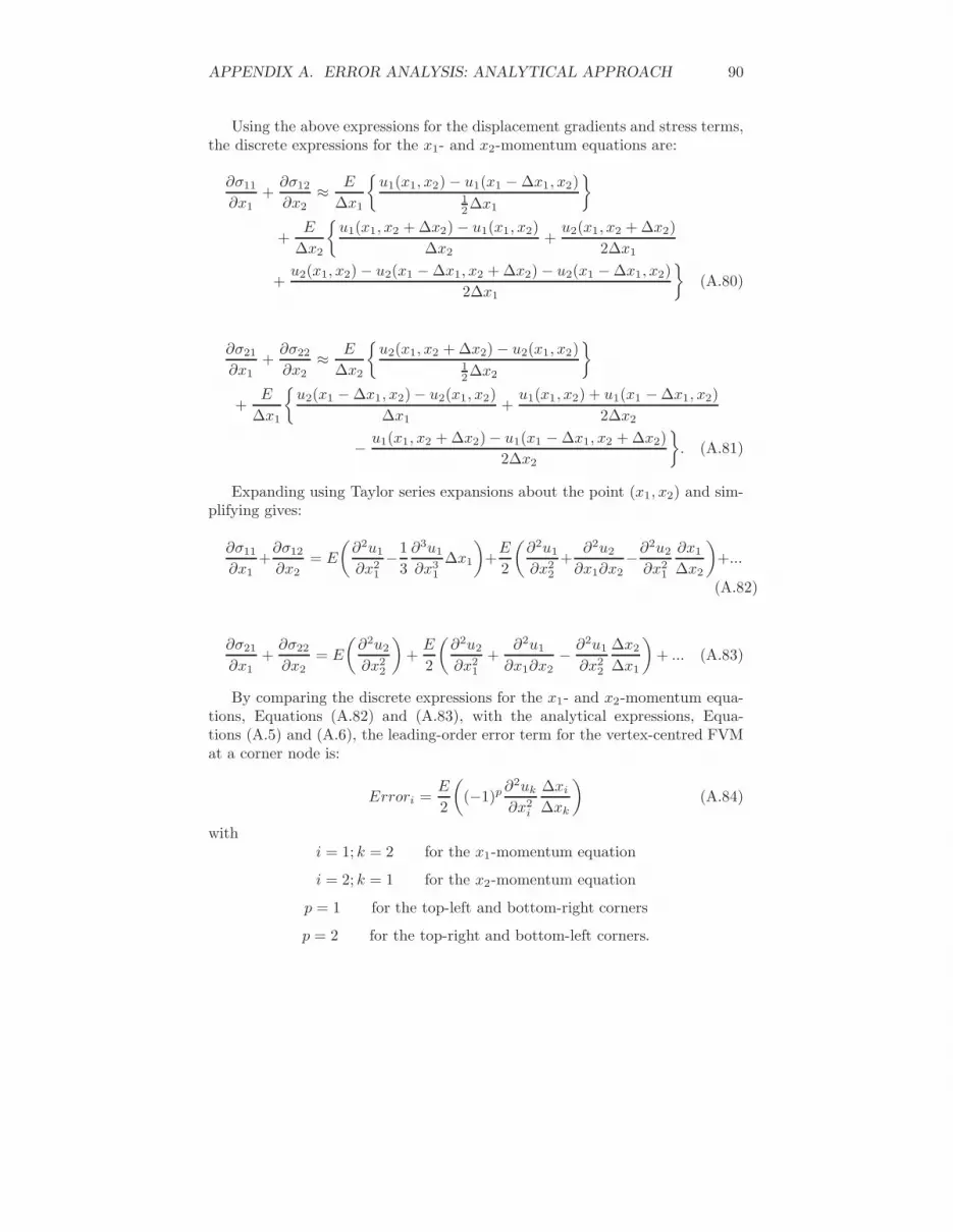
APPENDIX A. ERROR ANALYSIS: ANALYTICAL APPROACH 90

Using the above expressions for the displacement gradients and stress terms,the discrete expressions for the x1- and x2-momentum equations are:

∂σ11

∂x1+

∂σ12

∂x2≈ E

∆x1

{

u1(x1, x2) − u1(x1 − ∆x1, x2)12∆x1

}

+E

∆x2

{

u1(x1, x2 + ∆x2) − u1(x1, x2)

∆x2+

u2(x1, x2 + ∆x2)

2∆x1

+u2(x1, x2) − u2(x1 − ∆x1, x2 + ∆x2) − u2(x1 − ∆x1, x2)

2∆x1

}

(A.80)

∂σ21

∂x1+

∂σ22

∂x2≈ E

∆x2

{

u2(x1, x2 + ∆x2) − u2(x1, x2)12∆x2

}

+E

∆x1

{

u2(x1 − ∆x1, x2) − u2(x1, x2)

∆x1+

u1(x1, x2) + u1(x1 − ∆x1, x2)

2∆x2

− u1(x1, x2 + ∆x2) − u1(x1 − ∆x1, x2 + ∆x2)

2∆x2

}

. (A.81)

Expanding using Taylor series expansions about the point (x1, x2) and sim-plifying gives:

∂σ11

∂x1+

∂σ12

∂x2= E

(

∂2u1

∂x21

−1

3

∂3u1

∂x31

∆x1

)

+E

2

(

∂2u1

∂x22

+∂2u2

∂x1∂x2−∂2u2

∂x21

∂x1

∆x2

)

+...

(A.82)

∂σ21

∂x1+

∂σ22

∂x2= E

(

∂2u2

∂x22

)

+E

2

(

∂2u2

∂x21

+∂2u1

∂x1∂x2− ∂2u1

∂x22

∆x2

∆x1

)

+ ... (A.83)

By comparing the discrete expressions for the x1- and x2-momentum equa-tions, Equations (A.82) and (A.83), with the analytical expressions, Equa-tions (A.5) and (A.6), the leading-order error term for the vertex-centred FVMat a corner node is:

Errori =E

2

(

(−1)p ∂2uk

∂x2i

∆xi

∆xk

)

(A.84)

withi = 1; k = 2 for the x1-momentum equation

i = 2; k = 1 for the x2-momentum equation

p = 1 for the top-left and bottom-right corners

p = 2 for the top-right and bottom-left corners.

APPENDIX A. ERROR ANALYSIS: ANALYTICAL APPROACH 91

Corner Node - Hybrid FVM

Finally, for a corner node (Figure A.3) with the hybrid FVM, the elemental-based gradients are computed using Equation (3.53) as:

∂u1

∂x2

∣

∣

∣

∣

(x1,x2+12∆x2)

≈ ∂u1

∂x2

∣

∣

∣

∣

(x1−12∆x1,x2+

12∆x2)

≈ 1

2∆x2

[

u1(x1, x2 + ∆x2) − u1(x1, x2)

+ u1(x1 − ∆x1, x2 + ∆x2) − u1(x1 − ∆x1, x2)

]

(A.85)

∂u2

∂x1

∣

∣

∣

∣

(x1,x2+12∆x2)

≈ ∂u2

∂x1

∣

∣

∣

∣

(x1−12∆x1,x2+

12∆x2)

≈ 1

2∆x1

[

u2(x1, x2 + ∆x2) + u2(x1, x2)

− u2(x1 − ∆x1, x2 + ∆x2) − u2(x1 − ∆x1, x2)

]

(A.86)

∂u1

∂x2

∣

∣

∣

∣

(x1−12 ∆x1,x2)

≈ ∂u1

∂x2

∣

∣

∣

∣

(x1−12∆x1,x2+

12∆x2)

≈ 1

2∆x2

[

u1(x1, x2 + ∆x2) + u1(x1, x2)

+ u1(x1 + ∆x1, x2 + ∆x2) − u1(x1 − ∆x1, x2)

]

(A.87)

∂u2

∂x1

∣

∣

∣

∣

(x1+12∆x1,x2)

≈ ∂u2

∂x1

∣

∣

∣

∣

(x1−12 ∆x1,x2+

12∆x2)

≈ 1

2∆x1

[

u2(x1, x2 + ∆x2) − u2(x1 − ∆x1, x2 + ∆x2)

+ u2(x1 + ∆x1, x2) − u2(x1 − ∆x1, x2)

]

. (A.88)

Substituting these expressions for the displacement gradients gives the fol-

APPENDIX A. ERROR ANALYSIS: ANALYTICAL APPROACH 92

lowing discrete expressions for the for the x1- and x2-momentum equations:

∂σ11

∂x1+

∂σ12

∂x2≈ E

∆x1

{

u1(x1, x2) − u1(x1 − ∆x1, x2)12∆x1

}

E

2∆x2

{

u1(x1, x2 + ∆x2) + u1(x1 − ∆x1, x2 + ∆x2) − u1(x1, x2)

∆x2

− u1(x1 − ∆x1, x2)

∆x2+

u2(x1, x2 + ∆x2) − u2(x1 − ∆x1, x2 + ∆x2)

∆x1

+u2(x1, x2) − u2(x1 − ∆x1, x2)

∆x1

}

(A.89)

∂σ21

∂x1+

∂σ22

∂x2≈ E

∆x2

{

u2(x1, x2 + ∆x2) − u2(x1, x2)12∆x2

}

E

2∆x1

{

u2(x1 − ∆x1, x2 + ∆x2) + u2(x1 − ∆x1, x2) − u2(x1, x2)

∆x1

− u2(x1, x2 + ∆x2)

∆x1+

u1(x1 − ∆x1, x2) − u1(x1 − ∆x1, x2 + ∆x2)

∆x2

+u1(x1, x2) − u1(x1, x2 + ∆x2)

∆x2

}

. (A.90)

Expanding using Taylor series expansions about the point (x1, x2) and sim-plifying gives:

∂σ11

∂x1+

∂σ12

∂x2= E

(

∂2u1

∂x21

− 1

3

∂3u1

∂x31

∆x1

)

+E

2

(

∂2u1

∂x22

+∂2u2

∂x1∂x2

− ∂2u2

∂x21

∂x1

∆x2− ∂2u1

∂x1∂x2

∂x1

∆x2

)

+ ... (A.91)

∂σ21

∂x1+

∂σ22

∂x2= E

(

∂2u2

∂x22

)

+E

2

(

∂2u2

∂x21

+∂2u1

∂x1∂x2− ∂2u1

∂x22

∆x2

∆x1

− ∂2u2

∂x1∂x2

∆x2

∆x1

)

+ .... (A.92)

Comparing the discrete expressions for the x1- and x2-momentum equations,Equations (A.91) and (A.92), with the analytical expressions, Equations (A.5)and (A.6), gives the leading-order error term for the hybrid FVM at a cornernode:

Errori =E

2

(

(−1)p ∂2uk

∂x2i

∆xi

∆xk

− ∂2ui

∂xi∂xk

∆xi

∆xk

)

(A.93)

where the nomenclature is as previously defined.

Appendix B

Derivation of Third-Order

Gradient Approximation

The higher-order finite volume formulation uses third-order approximations forthe displacement gradients at boundary nodes. The derivation of this approxi-mation is shown in this section.

Consider a boundary node as shown in Figure B.1. To derive a third-orderapproximation for the gradient ∂u1

∂x2, we note that the the displacement values

over three elements are required. The form of the resulting equation is:

∂u1

∂x2≈ Au1(x1,x2)

+ Bu1(x1,x2+∆x2)+ Cu1(x1,x2+2∆x2)

+ Du1(x1,x2+3∆x2). (B.1)

Expanding each displacment term to third-order using Taylor series expan-sions about the point (x1, x2) gives:

Au1(x1,x2)= Au1 (B.2)

Bu1(x1,x2+∆x2)≈ Bu1 + B

∂u1

∂x1∆x2 + B

1

2

∂2u1

∂x22

∆x22 +

1

6B

∂3u1

∂x32

∆x32 (B.3)

Cu1(x1,x2+2∆x2)≈ Cu1 + 2C

∂u1

∂x1∆x2 + 2C

∂2u1

∂x22

∆x22 +

4

3C

∂3u1

∂x32

∆x32 (B.4)

Du1(x1,x2+3∆x2)≈ Du1 + 3D

∂u1

∂x1∆x2 +

9

2D

∂2u1

∂x22

∆x22 +

27

6D

∂3u1

∂x32

∆x32. (B.5)

Now, since we want a third-order approximation we note that:

A + B + C + D = 0 (B.6)

B + 2C + 3D = 1 (B.7)

1

2B + 2C +

9

2D = 0 (B.8)

93

APPENDIX B. DERIVATION OF THIRD-ORDER GRADIENT APPROXIMATION94

(x1, x2)

(x1, x2 + ∆x2)

(x1, x2 + 2∆x2)

(x1, x2 + 3∆x2)

∆x1∆x2

Figure B.1: Schematic of mesh indicating a boundary node at the bottomboundary of a beam

1

6B +

4

3C +

27

6D = 0. (B.9)

Solving the equations above simultaneously yields the following expression

for the gradient ∂u1

∂x2

∣

∣

∣

∣

(x1,x2)

:

∂u1

∂x2

∣

∣

∣

∣

(x1,x2)

≈−11u1(x1,x2)

+ 18u1(x1,x2+∆x2)− 9u1(x1,x2+2∆x2)

+ 2u1(x1,x2+3∆x2)

6∆x2.

(B.10)A similar approach is followed to obtain the remaining displacement gradient

approximations.

Bibliography

[1] B. Hubner, E. Walhorn, and D. Dinkler. A monolithic approach to fluid-structure interaction using space-time finite elements. Computer Methodsin Applied Mechanics and Engineering, 193:2087–2104, 2004.

[2] A.K. Slone, K. Pericleous, C. Bailey, M. Cross, and C. Bennett. A finitevolume unstructured mesh approach to dynamic fluid-structure interaction:an assessment of the challenge of predicting the onset of flutter. AppliedMathematical Modelling, 28:211–239, 2004.

[3] C. Farhat and M. Lesoinne. Two efficient staggered algorithms for theserial and parallel solution of three-dimensional nonlinear transient aeroe-lastic problems. Computer Methods in Applied Mechanics and Engineering,182:499–515, 2000.

[4] C.A. Taylor, T.J.R. Hughes, and C.K. Zarins. Finite element modellingof blood flow in arteries. Computer Methods in Applied Mechanics andEngineering, 158:155–196, 1998.

[5] J. Hron and M. Madlik. Fluid-structure interaction with applications inbiomechanics. Nonlinear Analysis: Real World Applications, 8:1431–1458,2007.

[6] J. De Hart, G.W.M. Peters, P.J.G. Schreurs, and F.P.T. Baaijens. A three-dimensional computational analysis of fluid-structure interaction in the aor-tic valve. Journal of Biomechanics, 36:101–112, 2003.

[7] K.-J. Paik, P.M. Carrica, D. Lee, and K. Maki. Strongly coupled fluid-structure interaction method for structural loads on surface ships. OceanEngineering, 36:1346–1357, 2009.

[8] K. Fujita. Flow-induced vibration and fluid-structure interaction in nu-clear power plant components. Journal of Wind Engineering and IndustrialAerodynamics, 33:405–418, 1990.

[9] A.C. Khanduri, T. Stathopoulos, and C. Bedard. Wind-induced interfer-ence effects on buildings – a review of the state-of-the-art. EngineeringStructures, 20:617–630, 1998.

95

BIBLIOGRAPHY 96

[10] W. Dettmer and J.D. Peric. A computational framework for fluid-structureinteraction: Finite element formulation and application. Computer Methodsin Applied Mechanics and Engineering, 195:5754–5779, 2006.

[11] C.J. Greenshields H.G. Weller. A unified formulation for continuum me-chanics applied to fluid-structure interaction in flexible tubes. InternationalJournal for Numerical Methods in Engineering, 64:1575–1593, 2005.

[12] K.J. Bathe and G.A. Ledezma. Benchmark problems for incompressiblefluid flows with structural interactions. Computers and Structures, 85:628–644, 2007.

[13] A.K. Slone, K. Pericleous, C. Bailey, and M. Cross. Dynamic fluid-structureinteraction using finite volume unstructured mesh procedures. Computersand Structures, 80:371–390, 2002.

[14] G. Xia and C.-L. Lin. An unstructured finite volume approach for structuraldynamics in response to fluid motions. Computers and Structures, 86:684–701, 2008.

[15] A. G. Malan. Investigation into the Continuum Thermodynamic Modelingof Investment Casting Shell-Mould Drying. PhD thesis, University of WalesSwansea, 2002.

[16] A.G. Malan and R.W. Lewis. An artificial compressibility CBS method formodelling heat transfer and fluid flow in heterogeneous porous materials.International Journal for Numerical Methods in Engineering, 87:412–423,2011.

[17] O.F. Oxtoby, A.G. Malan, and P. Nithiarasu. A novel matrix free, edgebased finite volume method for partitioned solution of fluid-structure in-teraction problems. International Journal for Numerical Methods in Engi-neering, submitted for review.

[18] O. Oxtoby and A.G. Malan. A 3D, parallel fluid-structure interaction code.In Proceedings of the 2nd African Conference on Computational MechanicsAn International Conference - AfriComp11, Cape Town, South Africa, 5-8January 2011.

[19] A.G. Malan and O. Oxtoby. A 3D parallel free-surface-modelling code forindustrial sloshing problems. In Proceedings of the 2nd African Conferenceon Computational Mechanics An International Conference - AfriComp11,Cape Town, South Africa, 5-8 January 2011.

[20] R. Suliman, O. Oxtoby, A.G. Malan, and S. Kok. An enhanced matrix-freeedge-based finite volume approach to model structures. In S. Kok, D.N.Wilke, and H.M. Inglis, editors, In proceedings: The 7th South AfricanConference on Computational and Applied Mechanics (SACAM10), pages399–406, Pretoria, South Africa, 10-13 January 2010.

BIBLIOGRAPHY 97

[21] O. C. Zienkiewicz and R. L. Taylor. The Finite Element Method: Volume1 - The Basis. Butterworth-Heinemann, Oxford, fifth edition, 2000.

[22] S. V. Patankar. Numerical Heat Transfer and Fluid Flow. McGraw-Hill,New York, 1980.

[23] E. Onate, M. Cervera, and O. C. Zienkiewicz. A finite-volume formatfor structural mechanics. International Journal for Numerical Methods inEngineering, 37:181–201, 1994.

[24] M.A. Wheel. A finite-volume approach to the stress analysis of pressurizedaxisymmetric structures. International Journal of Pressure Vessels andPiping, 68:311–317, 1996.

[25] J. Fainberg and H.-J. Leister. Finite volume multigrid solver for thermo-elastic stress analysis in anisotropic materials. Computer Methods in Ap-plied Mechanics and Engineering, 137:167–174, 1996.

[26] M.A. Wheel. A finite volume method for analysing the bending deformationof thick and thin plates. Computer Methods in Applied Mechanics andEngineering, 147:199–208, 1997.

[27] A.K. Slone, C. Bailey, and M. Cross. Dynamic solid mechanics using finitevolume methods. Applied Mathematical Modelling, 27:69–87, 2003.

[28] N. Fallah. A cell vertex and cell centred finite volume method for platebending analysis. Computer Methods in Applied Mechanics and Engineer-ing, 193:3457–3470, 2004.

[29] R.D. Cook, D.S. Malkus, M.E. Plesha, and R.J. Witt. Concepts and Ap-plications of Finite Element Analysis. John Wiley & Sons Ltd., UnitedStates, fourth edition, 2002.

[30] P. Wenke and M.A. Wheel. A finite volume method for solid mechanicsincorporating rotational degrees of freedom. Computers and Structures,81:321–329, 2003.

[31] N. Fallah, C. Bailey, M. Cross, and G.A. Taylor. Comparison of finiteelement and finite volume methods application in geometrically nonlinearstress analysis. Applied Mathematical Modelling, 24:439–455, 2000.

[32] M. Vaz Jr., P.A. Munoz-Rojas, and G. Filippini. On the accuracy of nodalstress computation in plane elasticity using finite volumes and finite ele-ments. Computers and Structures, 87:1044–1057, 2009.

[33] J.H. Ferziger and M. Peric. Computational Methods for Fluid Dynamics.Springer, third edition, 2002.

[34] J. Blazek. Computational Fluid Dynamics: Principles and Applications.Elsevier Science, Oxford, first edition, 2001.

BIBLIOGRAPHY 98

[35] X. Lv, Y. Zhao, X.Y. Huang, G.H. Xia, and X.H. Su. A matrix-free implicitunstructured multigrid finite volume method for simulating structural dy-namics and fluid-structure interaction. Journal of Computational Physics,225:120–144, 2007.

[36] Z.C He, G.R. Liu, Z.H. Zhong, G.Y. Zhang, and A.G. Cheng. Coupledanalysis of 3D structural-acoustic problems using the edge-based smoothedfinite element method/finite element method. Finite Elements in Analysisand Design, 46:1114–1121, 2010.

[37] S. Mitra and K.P. Sinhamahapatra. 2D simulation of fluid-structure in-teraction using finite element method. Finite Elements in Analysis andDesign, 45:52–59, 2008.

[38] T.E. Tezduyar, S. Sathe, R. Keedy, and K. Stein. Space-time finite ele-ment techniques for computation of fluid-structure interactions. ComputerMethods in Applied Mechanics and Engineering, 195:2002–2027, 2006.

[39] P.R.F. Texeira and A.M. Awruch. Numerical simulation of fluid-structureinteraction using the finite element method. Computers and Fluids, 34:249–273, 2005.

[40] J. Degroote, R. Haelterman, S. Annerel, P. Bruggeman, and J. Vieren-deels. Performance of partitioned procedures in fluid-structure interaction.Computers and Structures, 88:446–457, 2010.

[41] M. von Scheven and E. Ramm. Strong coupling schemes for interaction ofthin-walled structures and incompressible flows. International Journal forNumerical Methods in Engineering, 87:214–231, 2011.

[42] U. Kuttler and W. A. Wall. Fixed-point fluid–structure interaction solverswith dynamic relaxation. Computational Mechanics, 43:61–72, 2008.

[43] W. A. Wall, S. Genkinger, and E. Ramm. A strong coupling partitionedapproach for fluid–structure interaction with free surfaces. Computers andFluids, 36:169–183, 2007.

[44] D. P. Mok and W. A. Wall. Partitioned analysis schemes for the transientinteraction of incompressible flows and nonlinear flexible structures. InW. A. Wall and K.-U. Bletzinger, editors, Trends in computational struc-tural mechanics, pages 689–698, Barcelona: CIMNE, 2011.

[45] P. Le Tallec and J. Mouro. Fluid structure interaction with large structuraldisplacements. Computer Methods in Applied Mechanics and Engineering,190:3039–3067, 2001.

[46] H. G. Matthies and J. Steindorf. Partitioned strong coupling algorithms forfluid–structure interaction. Computers and Structures, 81:805–812, 2003.

BIBLIOGRAPHY 99

[47] J. Vierendeels, L. Lanoye, J. Degroote, and P. Verdonck. Implicit couplingof partitioned fluid-structure interaction problems with reduced order mod-els. Computers and Structures, 85:970–976, 2007.

[48] J. Degroote, K. J. Bathe, and J. Vierendeels. Performance of a new parti-tioned procedure versus a monolithic procedure in fluid-structure interac-tion. Computers and Structures, 87:793–801, 2009.

[49] G.A. Holzapfel. Nonlinear Solid Mechanics: A continuum Approach forEngineering. John Wiley & Sons Ltd., West Sussex, England, 2001.

[50] O. C. Zienkiewicz and R. L. Taylor. The Finite Element Method: Volume2 - Solid Mechanics. Butterworth-Heinemann, Oxford, fifth edition, 2000.

[51] R. Lohner. Applied CFD Techniques. John-Wiley and Sons Ltd., Chich-ester, 2001.

[52] Y. Zhao and B. Zhang. A high-order characteristics upwind FV method forincompressible flow and heat transfer simulation on unstructured grids. In-ternational Journal for Numerical Methods in Engineering, 37:3323–3341,1994.

[53] I. Bijelonja, I. Demirdzic, and S. Muzaferija. A finite volume method forincompressible linear elasticity. Computer Methods in Applied Mechanicsand Engineering, 195:6378–6390, 2006.

[54] W. Pan, M.A. Wheel, and Y. Qin. Six-node triangle finite volume methodfor solids with a rotational degree of freedom for incompressible material.Computers and Structures, 88:1506–1511, 2010.

[55] G.A. Taylor, C. Bailey, and M. Cross. Solution of the elastic/visco-plasticconstitutive equations: A finite volume approach. Applied MathematicalModelling, 19:746–760, 1995.

[56] G.A. Taylor, C. Bailey, and M. Cross. A vertex-based finite volume methodapplied to non-linear material problems in computational solid mechanics.International Journal for Numerical Methods in Engineering, 56:507–529,2003.

[57] S. Kok. Class notes MSY 411 continuum mechanics notes. Department ofMechanical and Aeronautical Engineering, University of Pretoria, February2007.

[58] P. I. Crumpton, P. Moinier, and M. B. Giles. An unstructured algorithmfor high Reynolds number flows on highly stretched meshes. In C. Taylorand J. T. Cross, editors, Numerical Methods in Laminar and TurbulentFlow, pages 561–572. Pineridge Press, 1997.

[59] A. G. Malan and R. W. Lewis. Modeling coupled heat and mass transferin drying non-hygroscopic capillary particulate materials. Communicationsin Numerical Methods in Engineering, 19(9):669–677, 2003.

BIBLIOGRAPHY 100

[60] A. Jameson. Time dependent calculations using multigrid, with applica-tions to unsteady flows past airfoils and wings. AIAA Paper, 91-1596,1991.

[61] V. Venkatakrishnan and D. J. Mavriplis. Implicit method for the compu-tation of unsteady flows on unstructured grids. Journal of ComputationalPhysics, 127:380–397, 1996.

[62] T. Belendez, C. Neipp, and A. Belendez. Large and small deflections of acantilever beam. European Journal of Physics, 23:371–379, 2002.

[63] C.W. Hirt, A.A. Amsden, and J.L. Cook. An arbitrary Lagrangian-Euleriancomputing method for all flow speeds. Journal of Computational Physics,14:227–253, 1974.

[64] O.F. Oxtoby and A.G. Malan. A matrix-free, implicit, incompressiblefractional-step algorithm for fluid-structure interaction applications. Jour-nal of Computational Physics, submitted for review.

[65] C. Farhat, M. Lesoinne, and P. LeTallec. Load and motion transfer algo-rithms for fluid/structure interaction problems with non-matching discreteinterfaces: Momentum and energy conservation, optimal discretization andapplication to aeroelasticity. Computer Methods in Applied Mechanics andEngineering, 157:95–114, 1998.

[66] A. de Boer, A.H. van Zuijlen, and H. Bijl. Review of coupling methodsfor non-matching meshes. Computer Methods in Applied Mechanics andEngineering, 196:1515–1525, 2007.

[67] G. Karypis and V. Kumar. A fast and high quality multilevel schemefor partitioning irregular graphs. SIAM Journal on Scientific Computing,20(1):359–392, 1999.

[68] W. Wall. Fluid-struktur-interaktion mit stabilisierten finiten elementen.PhD thesis, Universitat Stuttgart, 1999.