Embed Size (px)
Citation preview
DEVELOPMENT OF
PAVEMENT DESIGN CONCEPTS
Prepared for:
METROPOLITAN GOVERNMENT PAVEMENT ENGINEERS COUNCIL
Job No. 24,442 February 5, 1998

MGPEC VOL. II FEBRUARY 5, 1998 CTL/T 24,442
TABLE OF CONTENTS PURPOSE AND SCOPE.................................................................................................1
Acknowledgments ...........................................................................................................1
BACKGROUND ..............................................................................................................2
PRELIMINARY STUDIES................................................................................................3
DESIGN TRAFFIC ..........................................................................................................3
VEHICLE TYPES............................................................................................................4
Automobiles ....................................................................................................................4
Trucks and Buses ...........................................................................................................4
Construction Traffic .........................................................................................................6
DESIGN TRAFFIC EQUATIONS.....................................................................................8
Residential Streets ..........................................................................................................9
Commercial Streets.......................................................................................................10
Industrial Streets ...........................................................................................................11
Arterials.........................................................................................................................12
AXLE LOADS................................................................................................................14
TIRE-RELATED STRESSES ........................................................................................15
Summary.......................................................................................................................19
MATERIALS..................................................................................................................19
CONVENTIONAL TESTING..........................................................................................20
Resilient Modulus..........................................................................................................21
Moisture Content Effects ...............................................................................................23
Resilient Modulus Correlation for Subgrade Soils..........................................................24
Stabilized Subgrade ......................................................................................................29
Aggregate Base ............................................................................................................30
Asphalt Cement Concrete Pavement ............................................................................31
SWELLING SOILS ........................................................................................................32
Characterization ............................................................................................................33
Swell Mitigation Recommendations...............................................................................36
DRAINAGE ...................................................................................................................37
PAVEMENT DESIGN EQUATIONS..............................................................................39
MGPEC VOL. II FEBRUARY 5, 1998 CTL/T 24,442
Flexible Design Sensitivity Analysis...............................................................................39
Asphalt Pavement Parametric Studies ..........................................................................41
Flexible Pavement Design.............................................................................................45
Rigid Design Sensitivity Analysis...................................................................................47
Rigid Pavement Design.................................................................................................49
Design of Arterial Roadway...........................................................................................51
PAVEMENT MAINTENANCE........................................................................................52
Pavement Life Curves ...................................................................................................53
Pavement Maintenance Strategies................................................................................54
LIFE-CYCLE COST ANALYSIS ....................................................................................56
Discount Rate................................................................................................................58
Cost Definition...............................................................................................................58
Analysis Period .............................................................................................................59
Salvage Value ...............................................................................................................59
Life of Maintenance Treatments ....................................................................................59
Sensitivity Analyses.......................................................................................................61
CONCLUSION ..............................................................................................................61
REFERENCES
APPENDIX A - SURVEY RESULTS
APPENDIX B - GLOSSARY OF TERMS
APPENDIX C - ANNOTATED LITERATURE REVIEW
APPENDIX D - WARRANTIES AND QUALITY ASSURANCE / QUALITY CONTROL
APPENDIX E - MATERIAL TEST RESULTS

MGPEC VOL. II FEBRUARY 5, 1998 CTL/T 24,442
1
PURPOSE AND SCOPE
The Steering Committee of the Metropolitan Government Pavement Engineers
Council (MGPEC) desired to secure engineering and technical support to develop
standard pavement design and construction methodology for its member agencies. The
purpose of this document is to provide technical support for the companion Pavement
Design and Construction Manual and does not serve as a design document. Technical,
performance, and analytical data are presented in the form of charts, graphs, and
discussions. This report discusses traffic, materials, analysis procedures and results,
design equations, and life-cycle cost. Included as appendices are survey results
conducted to determine the state-of-practice, a glossary of terms, annotated literature
review, a discussion of QA/QC and warranty issues, and material test results. The
primary tasks focused on the characterization of pavement subgrade materials using
Resilient Modulus (Mr) testing, development of a pavement thickness design method for
new pavements, and creation of a uniform set of pavement construction specifications
for the Denver metropolitan area, exclusive from urban streets. It is believed that when
the design process and quality measurements recommended in the Pavement Design
and Construction Manual are implemented, future projects will yield better-performing
and longer-lasting roadways at an overall reduced life-cycle cost.
The scope of the study was based upon a contract between CTL/Thompson,
Inc., and the Colorado Department of Transportation (CDOT). The contract was
administered by CDOT for local agencies represented by a steering committee
composed of members of the Metropolitan Government Pavement Engineers Council
(MGPEC). The project was funded in cooperation by the Colorado Transportation
Institute (CTI), and Federal Highway Administration (FHWA) through Denver Regional
Council of Governments (DRCOG).
Acknowledgments
We would like to acknowledge and thank members of the Metropolitan
Government Pavement Engineers Council Steering Committee and the Review Panel for
MGPEC VOL. II FEBRUARY 5, 1998 CTL/T 24,442
2
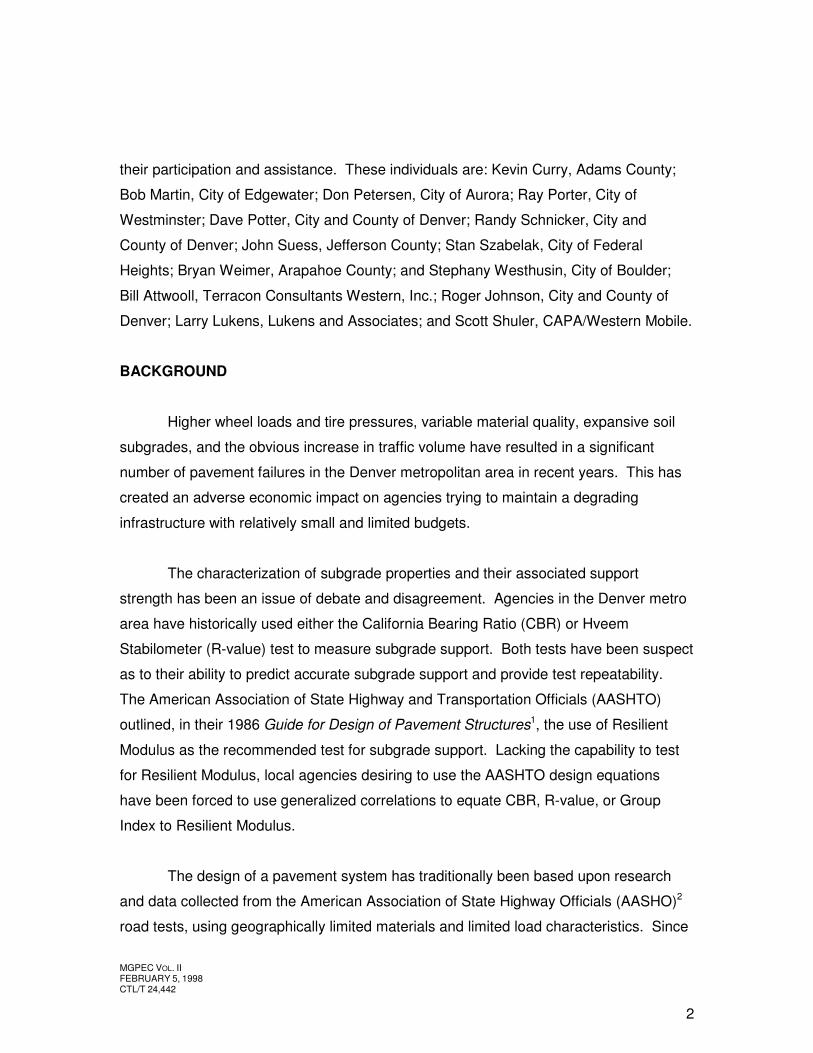
their participation and assistance. These individuals are: Kevin Curry, Adams County;
Bob Martin, City of Edgewater; Don Petersen, City of Aurora; Ray Porter, City of
Westminster; Dave Potter, City and County of Denver; Randy Schnicker, City and
County of Denver; John Suess, Jefferson County; Stan Szabelak, City of Federal
Heights; Bryan Weimer, Arapahoe County; and Stephany Westhusin, City of Boulder;
Bill Attwooll, Terracon Consultants Western, Inc.; Roger Johnson, City and County of
Denver; Larry Lukens, Lukens and Associates; and Scott Shuler, CAPA/Western Mobile.
BACKGROUND
Higher wheel loads and tire pressures, variable material quality, expansive soil
subgrades, and the obvious increase in traffic volume have resulted in a significant
number of pavement failures in the Denver metropolitan area in recent years. This has
created an adverse economic impact on agencies trying to maintain a degrading
infrastructure with relatively small and limited budgets.
The characterization of subgrade properties and their associated support
strength has been an issue of debate and disagreement. Agencies in the Denver metro
area have historically used either the California Bearing Ratio (CBR) or Hveem
Stabilometer (R-value) test to measure subgrade support. Both tests have been suspect
as to their ability to predict accurate subgrade support and provide test repeatability.
The American Association of State Highway and Transportation Officials (AASHTO)
outlined, in their 1986 Guide for Design of Pavement Structures1, the use of Resilient
Modulus as the recommended test for subgrade support. Lacking the capability to test
for Resilient Modulus, local agencies desiring to use the AASHTO design equations
have been forced to use generalized correlations to equate CBR, R-value, or Group
Index to Resilient Modulus.
The design of a pavement system has traditionally been based upon research
and data collected from the American Association of State Highway Officials (AASHO)2
road tests, using geographically limited materials and limited load characteristics. Since
MGPEC VOL. II FEBRUARY 5, 1998 CTL/T 24,442
3
the mid-1970s, changes in traffic loadings, tire pressures, and quality of materials have
made it necessary to modify the design process.
Once a roadway is constructed, maintenance becomes the critical factor in the
long-term serviceability of a pavement system. A properly planned and implemented
maintenance program is necessary to extend the design life of any pavement system.
Included in this document are a life-cycle cost analysis and recommendations for
maintaining asphalt and concrete pavements.
PRELIMINARY STUDIES
A state-of-practice survey (Appendix A) was performed to assist in determining
the direction of the study. Survey data suggest base failures, thermal and fatigue
cracking, and rutting are the most common maintenance problems in the Denver metro
area. All of the agencies require a form of the 1986 AASHTO design procedure for
design of new pavements and also have specifications for asphalt mixes. Forty percent
have lime-stabilization specifications. Only 50 percent have a Pavement Management
System (PMS).
As part of the research effort, a Glossary of Terms was developed to standardize
the technical language and reduce confusion. The Glossary is presented in Appendix B.
Appendix C contains an annotated review of the literature conducted as part of this
effort. Appendix D contains a discussion of QA/QC and warranty issues pertaining to
testing requirements and penalties.
DESIGN TRAFFIC
Traffic loads are the basis for determining the structural requirements of any
rational pavement design. The original AASHO and subsequent AASHTO3 design
methodologies use the concept of pavement serviceability related to “Equivalent” 18 kip
Single Axle Loads over a twenty-year service period (ESAL20). The critical factors in
design are traffic volume, wheel load, and subgrade support. As wheel loads and tire
pressures increase, damage to pavement increases exponentially. Traffic volume has a
MGPEC VOL. II FEBRUARY 5, 1998 CTL/T 24,442
4
similar degrading effect on pavement life and serviceability. As part of this traffic study,
a significant level of effort was expended to quantify traffic loads and to develop rational
pavement loading based upon anticipated traffic for each pavement roadway land use
classification (i.e., residential, commercial, industrial, and arterial).
VEHICLE TYPES
The loads transmitted to the pavement surface are dependent upon tire types,
axle weight, gross vehicle weight, tire pressure, and axle configuration. Loads
transmitted to the pavement are dependent on the type of tire, i.e. radial or bias-ply. In
the process of categorizing traffic load, typical vehicle configurations were analyzed.
Axle and tire configurations and gross vehicle weights were used to model each
roadway pavement, based upon roadway land use classification, in the development of
the design traffic equations.
Automobiles
The most prevalent volume of traffic on any pavement surface is from
automobiles. Owing to the relatively light weight and low tire pressure, a single
automobile causes insignificant measurable damage to the pavement structure. This is
reflected by the load equivalent factors used by AASHTO,3 equating an auto load to
approximately 0.0002 of a single 18,000-pound axle load. This value indicates
approximately 5,000 automobiles are required to equate to one ESAL20. Automobile
loads were considered in the design traffic calculations for this study, even though their
effect is insignificant.
Trucks and Buses
Heavier loads, such as delivery trucks, garbage trucks, buses, and tractor-trailer
trucks, are the most significant loads on most pavement surfaces. The Regional
Transportation District (RTD) operates multiple bus units on daily routes throughout the
Denver metro area. Based upon AASHTO Load Equivalent Factors, a single RTD bus
MGPEC VOL. II FEBRUARY 5, 1998 CTL/T 24,442
5
can load a pavement structure equal to the load from 19,240 automobiles, whereas the
load from one heavy H-20 truck can be equal to 64,235 automobiles.
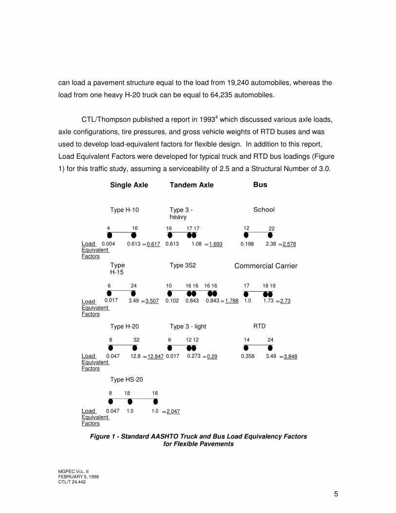
CTL/Thompson published a report in 19934 which discussed various axle loads,
axle configurations, tire pressures, and gross vehicle weights of RTD buses and was
used to develop load-equivalent factors for flexible design. In addition to this report,
Load Equivalent Factors were developed for typical truck and RTD bus loadings (Figure
1) for this traffic study, assuming a serviceability of 2.5 and a Structural Number of 3.0.
Figure 1 - Standard AASHTO Truck and Bus Load Equivalency Factors for Flexible Pavements
Single Axle Tandem Axle Bus
32
1818
8
8
1616
6 24
4 17 17
1710
14 24
18 19
12 22
16 16 16 16
Type 3 - heavy
Type H-10
Type H-15
Type H-20
Type HS-20
Type 3S2
School
RTD
0.004 0.613 = 0.617
0.017 3.49 = 3.507
Load Equivalent Factors
Load Equivalent Factors
Load Equivalent Factors
Load Equivalent Factors
0.047 12.8 = 12.847
0.047 1.0 1.0 = 2.047
0.613 1.08 = 1.693
0.102
0.198
1.0
0.358
0.843 0.843
2.38
1.73
3.49
= 1.788
= 2.578
= 2.73
= 3.848
Type 3 - light
6 12 12
0.017 0.273 = 0.29
Commercial Carrier
MGPEC VOL. II FEBRUARY 5, 1998 CTL/T 24,442
6
Trash trucks are the most common heavy-load vehicles and are likely the
heaviest and most damaging loads to residential pavement structures. Trash trucks are
typically either two- or three-axle, single-unit trucks. Most trash trucks are either 30,000-
pound trucks with a 24,000-pound single-axle load (Type H-15) or 50,000-pound trucks
with two rear axles at 18,000 pounds each (Type 3-Heavy). For design purposes, the
Type 3-heavy trash truck should be used, because it is the most common trash truck.
Construction Traffic
Construction traffic loads are not considered in the design of new pavement
systems, particularly for residential pavements. Construction traffic includes numerous
heavily loaded trucks for concrete, drywall, brick, framing, and sod delivery. For
residential streets, the construction period represents the highest concentration of loads
imposed on the pavement during its service life and must be considered as a design
factor.
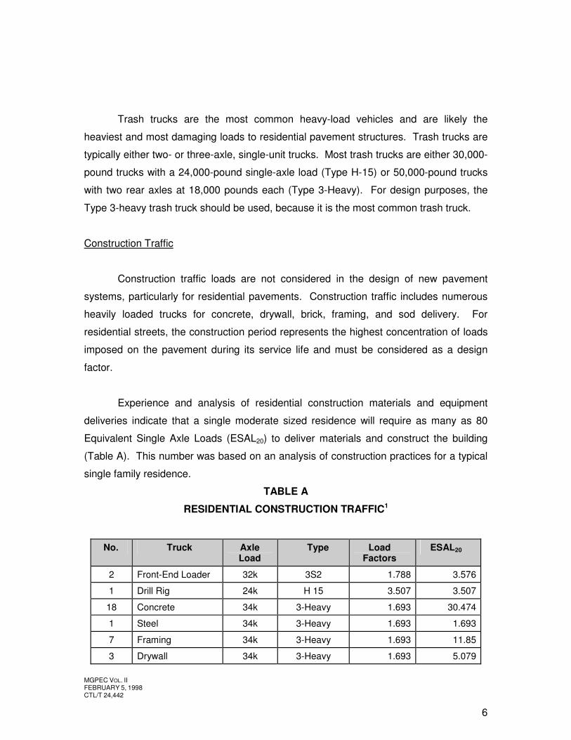
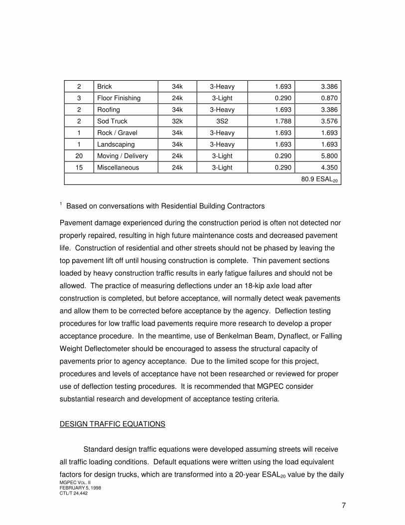
Experience and analysis of residential construction materials and equipment
deliveries indicate that a single moderate sized residence will require as many as 80
Equivalent Single Axle Loads (ESAL20) to deliver materials and construct the building
(Table A). This number was based on an analysis of construction practices for a typical
single family residence.
TABLE A
RESIDENTIAL CONSTRUCTION TRAFFIC1
No. Truck Axle Load
Type Load Factors
ESAL20
2 Front-End Loader 32k 3S2 1.788 3.576
1 Drill Rig 24k H 15 3.507 3.507
18 Concrete 34k 3-Heavy 1.693 30.474
1 Steel 34k 3-Heavy 1.693 1.693
7 Framing 34k 3-Heavy 1.693 11.85
3 Drywall 34k 3-Heavy 1.693 5.079
MGPEC VOL. II FEBRUARY 5, 1998 CTL/T 24,442
7
2 Brick 34k 3-Heavy 1.693 3.386
3 Floor Finishing 24k 3-Light 0.290 0.870
2 Roofing 34k 3-Heavy 1.693 3.386
2 Sod Truck 32k 3S2 1.788 3.576
1 Rock / Gravel 34k 3-Heavy 1.693 1.693
1 Landscaping 34k 3-Heavy 1.693 1.693
20 Moving / Delivery 24k 3-Light 0.290 5.800
15 Miscellaneous 24k 3-Light 0.290 4.350
80.9 ESAL20
1 Based on conversations with Residential Building Contractors Pavement damage experienced during the construction period is often not detected nor
properly repaired, resulting in high future maintenance costs and decreased pavement
life. Construction of residential and other streets should not be phased by leaving the
top pavement lift off until housing construction is complete. Thin pavement sections
loaded by heavy construction traffic results in early fatigue failures and should not be
allowed. The practice of measuring deflections under an 18-kip axle load after
construction is completed, but before acceptance, will normally detect weak pavements
and allow them to be corrected before acceptance by the agency. Deflection testing
procedures for low traffic load pavements require more research to develop a proper
acceptance procedure. In the meantime, use of Benkelman Beam, Dynaflect, or Falling
Weight Deflectometer should be encouraged to assess the structural capacity of
pavements prior to agency acceptance. Due to the limited scope for this project,
procedures and levels of acceptance have not been researched or reviewed for proper
use of deflection testing procedures. It is recommended that MGPEC consider
substantial research and development of acceptance testing criteria.
DESIGN TRAFFIC EQUATIONS
Standard design traffic equations were developed assuming streets will receive
all traffic loading conditions. Default equations were written using the load equivalent
factors for design trucks, which are transformed into a 20-year ESAL20 value by the daily
MGPEC VOL. II FEBRUARY 5, 1998 CTL/T 24,442
8
traffic volume and the constant value of 7,300 (assuming a 20-year design life and 365
days in one year). No growth factor is considered since the traffic numbers are
estimated for total “build-out” volume. The pavement design procedure is dependent
upon the accuracy of traffic studies and load equivalency predictions. Tire pressures
and stresses should be considered in the development of load equivalent factors to
provide the most reliable pavement design possible. The trucks used in these equations
were chosen as typical vehicles expected in the corresponding roadway land use
classifications.
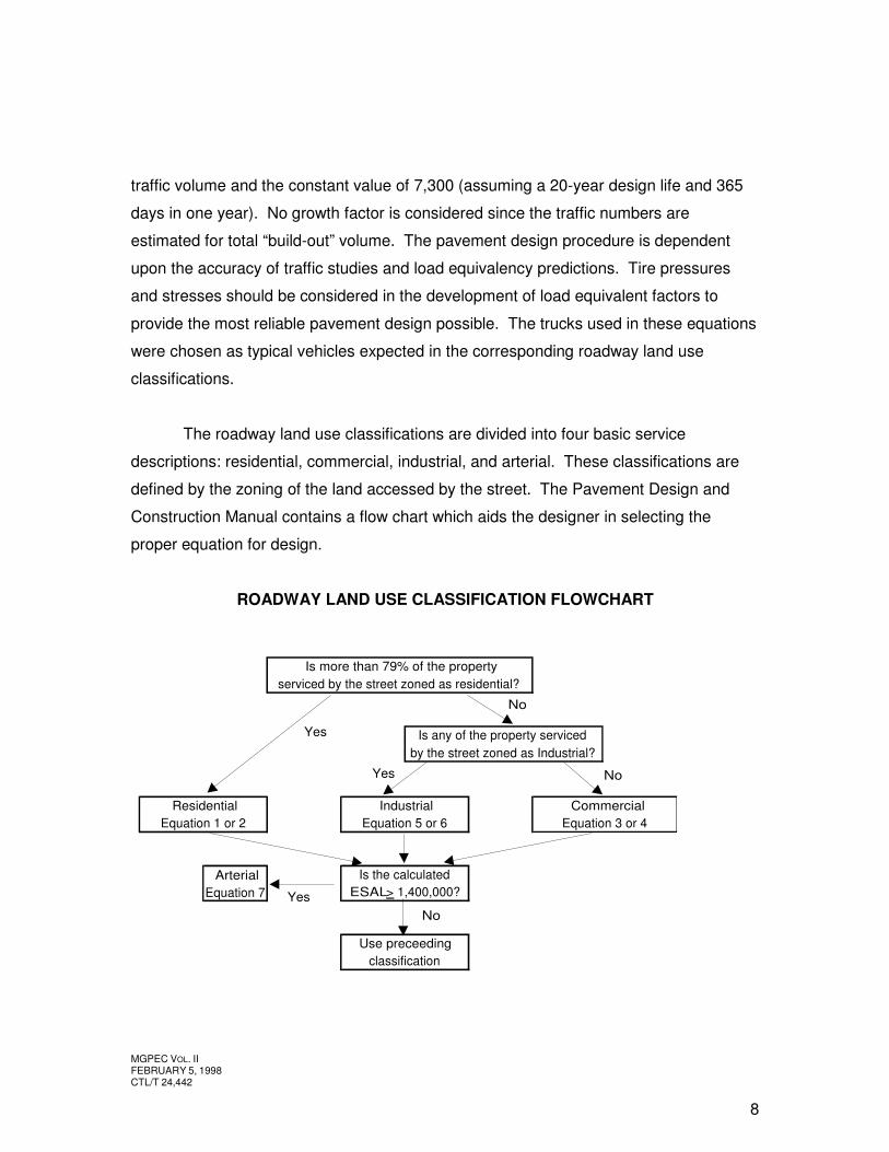
The roadway land use classifications are divided into four basic service
descriptions: residential, commercial, industrial, and arterial. These classifications are
defined by the zoning of the land accessed by the street. The Pavement Design and
Construction Manual contains a flow chart which aids the designer in selecting the
proper equation for design.
ROADWAY LAND USE CLASSIFICATION FLOWCHART
Is more than 79% of the property serviced by the street zoned as residential?
Is any of the property servicedby the street zoned as Industrial?
Residential Industrial CommercialEquation 1 or 2 Equation 5 or 6 Equation 3 or 4
Arterial Is the calculatedEquation 7 ESAL > 1,400,000?
Use preceeding classification
Yes
No
No
YesNo
Yes
MGPEC VOL. II FEBRUARY 5, 1998 CTL/T 24,442
9
Residential Streets
The majority of the traffic on residential streets consists of light automobiles.
Residential areas rarely receive heavy loads other than trash trucks, construction traffic,
and school buses. Residential streets are defined as those having less than 20 percent
of the area served zoned as commercial property.
These values are formatted into design Equation 1, as shown below.
Equation 1: ESAL20 = [(a)(2.578) + (b)(1.693) + (c)(0.0002)] 7300 + 80 (R) where: a = number of school buses per day b = number of Type 3-Heavy trash trucks per day c = number of automobiles per day R = number of residential density units serviced by the street The default equation for residential streets was developed using the applicable
traffic loads. A typical residential street is expected to receive:
< two school buses per day (a)
< two Type 3-Heavy trash trucks per day (b)
< five-hundred automobiles per day (c)
Using the estimated traffic volumes for residential streets, the default Equation 2 was
reduced as:
Equation 2; default Residential: ESAL20 = 62,000 + 80 (R) where: R = number of residential density units serviced by the street Commercial Streets
Commercial streets provide access to retail stores, businesses, offices, and other
commercial areas. The definition of a commercial street is one where more than 20
percent of the land served is zoned as non residential. These streets typically receive a
large mix of residential traffic along with trash services and delivery trucks. The number
MGPEC VOL. II FEBRUARY 5, 1998 CTL/T 24,442
10
of garbage and delivery trucks generally determines the structural requirements of these
streets. The standard equation for commercial streets is developed as:
Equation 3: ESAL20 = 62,000 + 80 (R) + [(a)(2.578) + (b)(1.693) + (c)(0.0002) + (d)(0.617) + (e)(3.848) + (f)(1.788) + (g)(2.047)] 7300 where: a = number of school buses per day b = number of Type 3-Heavy trash trucks per day c = number of automobiles per day d = number of Type H-10, light two-axle trucks per day e = number of RTD buses per day f = number of Type 3S2, tractor-trailer trucks per day g = number of Type HS-20, three-axle trucks per day R = number of residential density units serviced by the street Typical traffic volume was estimated for a one-acre commercial fill-in property
surrounded by developments, similar to a strip shopping center, with a 20,000 square-
foot facility on the property. It was estimated a commercial site will include:
< two school buses per day (a) < two Type 3-Heavy trash trucks per day (b) < one-thousand automobiles per day (c) < twelve Type H-10, light two-axle trucks per day (d) < two RTD buses per day (e) < two Type 3S2, tractor-trailer trucks per day (f) < four Type HS-20, three-axle trucks per day (g)
In addition, it was assumed the residential traffic was added to account for the residential
areas accessed by the street. The construction traffic loads for a commercial property
were considered, yet the loads did not exceed the expected daily traffic volume for a non
residential street. Therefore, the construction period is considered typical service not
warranting special consideration.
Using the estimated traffic volumes for one acre of commercial property, the
default commercial Equation 4 was reduced as:
Equation 4; default Commercial: ESAL20 = 62,000 + 80 (R) + 260,000 (CA)
MGPEC VOL. II FEBRUARY 5, 1998 CTL/T 24,442
11
where: R = number of residential density units serviced by the street CA = acres of commercial property serviced by the street Industrial Streets
Industrial streets are defined as streets having property zoned for industrial use
(manufacturing, distribution, warehousing, etc.). These streets will also receive some
commercial traffic. Industrial streets demand higher structural requirements primarily
due to the large number of multiple-unit trucks used for deliveries. The frequency of
trash trucks and buses also increase in industrial areas. Experience indicates
Equivalent Daily 18 kip axle loads can vary from less than 50 to over 1500 depending on
the use of the property. It is strongly recommended to require a full use traffic study for
each facility and require improvements accordingly.
Industrial streets are very similar to commercial streets yet are subject to an
increase in Type 3S2, tractor-trailer trucks. Industrial streets are often not associated
with residential areas, therefore the residential construction factor is not used in the
derivation of the default equation. Since industrial areas are often connected to
commercial areas, the equation should consider the commercial default traffic. The
following Equation 5 is developed for fill-in development of industrial streets:
Equation 5: ESAL20 = 260,000 (CA) + [(b)(1.693) + (c)(0.0002) + (e)(3.848) + (f)(1.788) + (g)(2.047)] 7300 where: CA = acres of commercial property services by the street b = number of Type 3-Heavy trash trucks per day c = number of automobiles per day e = number of RTD buses per day f = number of Type 3S2, tractor-trailer trucks per day g = number of Type HS-20, three trucks per day It was estimated that industrial lots would include:
< three Type 3-heavy trash trucks per day (b) < one-thousand automobiles per day (c) < two RTD buses per day (e)
MGPEC VOL. II FEBRUARY 5, 1998 CTL/T 24,442
12
< twenty Type 3S2, tractor-trailer trucks per day (f) < three Type HS-20, three-axle trucks per day (g)
Equation 6 was reduced using the estimated traffic volumes for one acre of
commercial and one acre of industrial property:
Equation 6; default Industrial: ESAL20 = 260,000 (CA) + 400,000 (IA) Where: CA = Acres of commercial property serviced by the street IA = Acres of industrial property serviced by the street Arterials
Arterials are roadways that serve as primary routes across the city, linking major
population, commercial, and industrial areas. They do not fall into one of the previously
discussed categories, or at a minimum, are found to be four-lane roads that service large
subdivisions, and/or commercial and industrial properties. Therefore, a detailed traffic
study should be performed for arterials.
The traffic study should address traffic volume, the distribution of truck types, and
the variations in traffic loading by lane. As a minimum, the traffic study should detail the
estimated number of automobiles, the number of residential units, and areas of
commercial and industrial areas served by the roadway. The study should estimate the
number of trucks of each type and the lane distribution. Buses should be considered a
definite probability on any major arterial, even if the current RTD plans do not include the
roadway. The design traffic should be calculated for lane-by-lane ESALs.
Because of the various functions of arterial streets (i.e., serving as major routes
to airports, trash or recycling centers, or residential parkways), their design ESAL20
should be calculated using Load Equivalency Factors and detailed 20-year traffic
projections. A typical range of ESALs20 is 300,000 to 3,000,000 or more and the design
should account for variations in lane loading in the traffic analysis.
MGPEC VOL. II FEBRUARY 5, 1998 CTL/T 24,442
13
For arterial streets, or in situations where the designer must develop a detailed
traffic study for a miscellaneous roadway use classification, Equation 7 should be used
to develop the design ESAL20. Equation 7 presents the design traffic equation with each
possible loading condition.
Equation 7: ESAL20 = [(a)(2.578) + (b)(1.693) + (c)(0.0002) + (d)(0.617) + (e)(3.848) + (f)(1.788) + (g)(2.047) + (h)(12.847) + (i)(3.507) + (j)(0.290) + (k)(2.73)]7300 + 80(R) where: a = number of school buses per day b = number of Type 3-Heavy trash trucks per day c = number of automobiles per day d = number of Type H-10, light two-axle delivery trucks per day e = number of RTD buses per day f = number of Type 3S2, tractor-dual trailer trucks per day g = number of Type HS-20, three-axle trucks per day h = number of Type H-20 trucks per day i = number of Type H-15 trucks per day j = number of Type 3-Light trucks per day k = number of Commercial Carrier buses per day R = number of residential lots serviced by the street
AXLE LOADS
A parametric study on axle loads and tire pressures was performed to determine
the effect of traffic loads on the fatigue life of a pavement system. These factors were
not considered as input variables into the AASHTO design equation. This evaluation
was not intended to change the design method, but was to provide a discussion of other
traffic loading variables. The study emphasizes the importance of load calculations and
shows internal pavement stresses are much higher than normally assumed. The
thickness design is not normally influenced by the tire pressures and loads, but more
accurate load equivalent factors and improved material properties can help counter
these stresses.
The DAMA program, by the Asphalt Institute,5 was used to perform the analysis.
The program analyzes multilayered elastic pavement structures by cumulative damage
MGPEC VOL. II FEBRUARY 5, 1998 CTL/T 24,442
14
techniques for single and dual wheel load systems. The program was chosen based on
results of research by Chen et al.6 that evaluated available computer programs for
pavement structural analysis. DAMA
is one of the best programs because it
analyzes most correctly the maximum
surface deflection, tensile strain at the
bottom of the asphalt layer, and
compressive strain at the top of the
subgrade. In addition, DAMA satisfies
the natural boundary conditions in
which the vertical stresses equal the
imposed contact pressure, and it
allows a single or dual wheel
configuration to be considered.
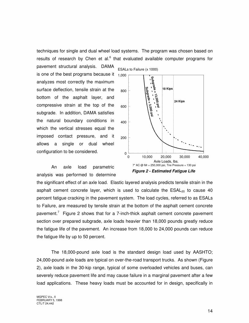
An axle load parametric
analysis was performed to determine
the significant effect of an axle load. Elastic layered analysis predicts tensile strain in the
asphalt cement concrete layer, which is used to calculate the ESAL20 to cause 40
percent fatigue cracking in the pavement system. The load cycles, referred to as ESALs
to Failure, are measured by tensile strain at the bottom of the asphalt cement concrete
pavement.7 Figure 2 shows that for a 7-inch-thick asphalt cement concrete pavement
section over prepared subgrade, axle loads heavier than 18,000 pounds greatly reduce
the fatigue life of the pavement. An increase from 18,000 to 24,000 pounds can reduce
the fatigue life by up to 50 percent.
The 18,000-pound axle load is the standard design load used by AASHTO;
24,000-pound axle loads are typical on over-the-road transport trucks. As shown (Figure
2), axle loads in the 30-kip range, typical of some overloaded vehicles and buses, can
severely reduce pavement life and may cause failure in a marginal pavement after a few
load applications. These heavy loads must be accounted for in design, specifically in
Figure 2 - Estimated Fatigue Life 7" AC @ Mr = 250,000 psi, Tire Pressure = 130 psi
0 10,000 20,000 30,000 40,0000
200
400
600
800
1,000
Axle Loads, lbs.
ESALs to Failure (x 1000)
Subgrade = 13,000 psi
Subgrade = 3,000 psi
18 Kips
24 Kips
MGPEC VOL. II FEBRUARY 5, 1998 CTL/T 24,442
15
bus lanes of arterial streets. These types
of loads are accounted for by use of the
Load Equivalency Factors shown on
Figure 1.
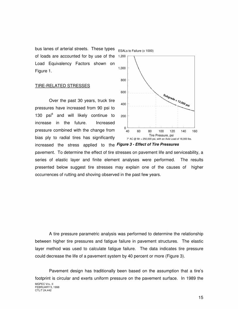
TIRE-RELATED STRESSES
Over the past 30 years, truck tire
pressures have increased from 90 psi to
130 psi8 and will likely continue to
increase in the future. Increased
pressure combined with the change from
bias ply to radial tires has significantly
increased the stress applied to the
pavement. To determine the effect of tire stresses on pavement life and serviceability, a
series of elastic layer and finite element analyses were performed. The results
presented below suggest tire stresses may explain one of the causes of higher
occurrences of rutting and shoving observed in the past few years.
A tire pressure parametric analysis was performed to determine the relationship
between higher tire pressures and fatigue failure in pavement structures. The elastic
layer method was used to calculate fatigue failure. The data indicates tire pressure
could decrease the life of a pavement system by 40 percent or more (Figure 3).
Pavement design has traditionally been based on the assumption that a tire’s
footprint is circular and exerts uniform pressure on the pavement surface. In 1989 the
Figure 3 - Effect of Tire Pressures 7" AC @ Mr = 250,000 psi, with an Axle Load of 18,000 lbs.
40 60 80 100 120 140 1600
200
400
600
800
1,000
1,200
Tire Pressure, psi
ESALs to Failure (x 1000)
Subgrade = 13,000 psi
MGPEC VOL. II FEBRUARY 5, 1998 CTL/T 24,442
16
Texas Transportation Institute (TTI)
conducted a study on tire pressure
distributions for the Air Force
Engineering and Services Center.9
The TTI study looked at pavement
pressure distributions produced by a
variety of radial and bias-ply tires used
by the Air Force aircraft. The wheel
loads and tire pressures used for this
study were similar to conventional
truck tires.
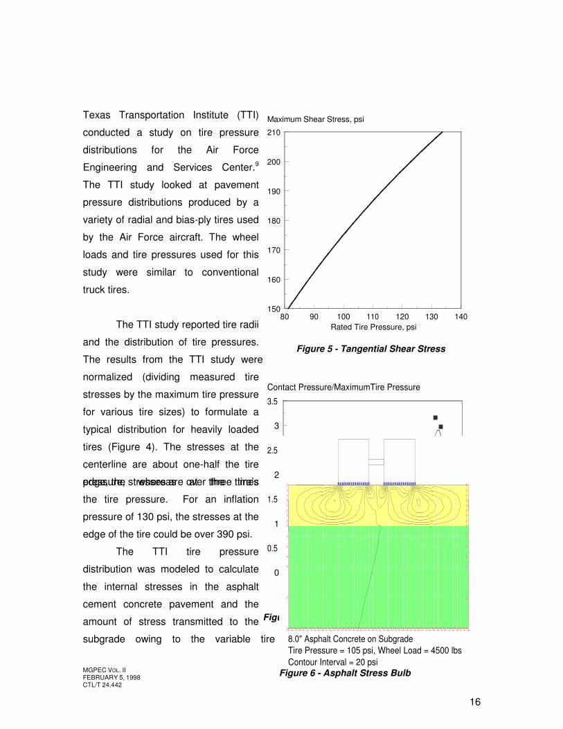
The TTI study reported tire radii
and the distribution of tire pressures.
The results from the TTI study were
normalized (dividing measured tire
stresses by the maximum tire pressure
for various tire sizes) to formulate a
typical distribution for heavily loaded
tires (Figure 4). The stresses at the
centerline are about one-half the tire
pressure, whereas at the tire’s edge, the stresses are over three times
the tire pressure. For an inflation
pressure of 130 psi, the stresses at the
edge of the tire could be over 390 psi.
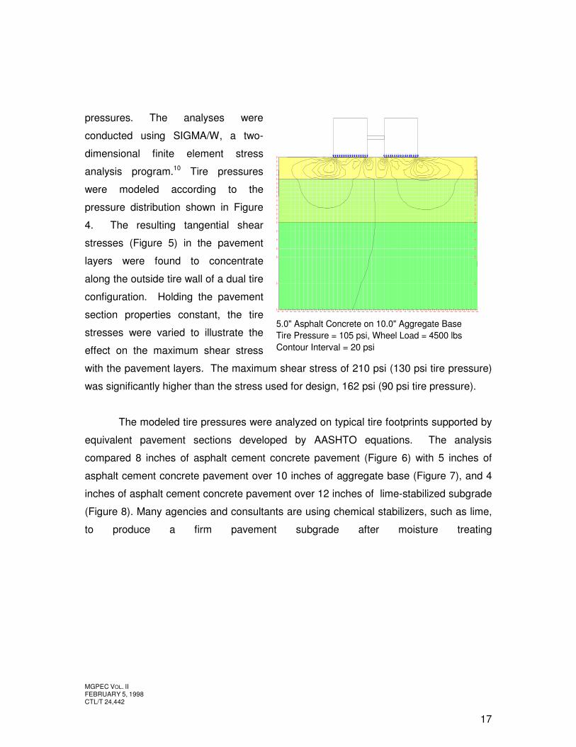
The TTI tire pressure
distribution was modeled to calculate
the internal stresses in the asphalt
cement concrete pavement and the
amount of stress transmitted to the
subgrade owing to the variable tire
Figure 4 - Tire Pressure Distribution
Figure 5 - Tangential Shear Stress
Figure 6 - Asphalt Stress Bulb
CL
0 0.2 0.4 0.6 0.8 10
0.5
1
1.5
2
2.5
3
3.5
Tire Footprint Radius from Mid-tire Centerline
Contact Pressure/MaximumTire Pressure
80 90 100 110 120 130 140150
160
170
180
190
200
210
Rated Tire Pressure, psi
Maximum Shear Stress, psi
8.0" Asphalt Concrete on SubgradeTire Pressure = 105 psi, Wheel Load = 4500 lbsContour Interval = 20 psi
MGPEC VOL. II FEBRUARY 5, 1998 CTL/T 24,442
17
pressures. The analyses were
conducted using SIGMA/W, a two-
dimensional finite element stress
analysis program.10 Tire pressures
were modeled according to the
pressure distribution shown in Figure
4. The resulting tangential shear
stresses (Figure 5) in the pavement
layers were found to concentrate
along the outside tire wall of a dual tire
configuration. Holding the pavement
section properties constant, the tire
stresses were varied to illustrate the
effect on the maximum shear stress
with the pavement layers. The maximum shear stress of 210 psi (130 psi tire pressure)
was significantly higher than the stress used for design, 162 psi (90 psi tire pressure).
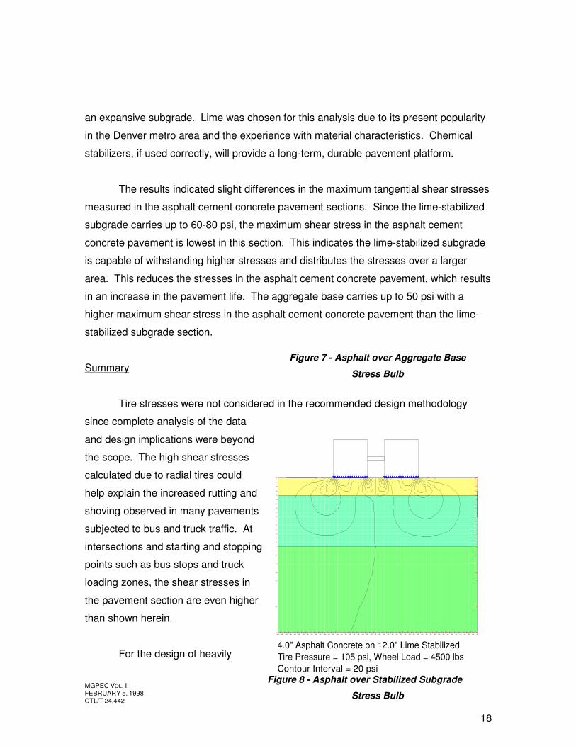
The modeled tire pressures were analyzed on typical tire footprints supported by
equivalent pavement sections developed by AASHTO equations. The analysis
compared 8 inches of asphalt cement concrete pavement (Figure 6) with 5 inches of
asphalt cement concrete pavement over 10 inches of aggregate base (Figure 7), and 4
inches of asphalt cement concrete pavement over 12 inches of lime-stabilized subgrade
(Figure 8). Many agencies and consultants are using chemical stabilizers, such as lime,
to produce a firm pavement subgrade after moisture treating
5.0" Asphalt Concrete on 10.0" Aggregate BaseTire Pressure = 105 psi, Wheel Load = 4500 lbsContour Interval = 20 psi
MGPEC VOL. II FEBRUARY 5, 1998 CTL/T 24,442
18
an expansive subgrade. Lime was chosen for this analysis due to its present popularity
in the Denver metro area and the experience with material characteristics. Chemical
stabilizers, if used correctly, will provide a long-term, durable pavement platform.
The results indicated slight differences in the maximum tangential shear stresses
measured in the asphalt cement concrete pavement sections. Since the lime-stabilized
subgrade carries up to 60-80 psi, the maximum shear stress in the asphalt cement
concrete pavement is lowest in this section. This indicates the lime-stabilized subgrade
is capable of withstanding higher stresses and distributes the stresses over a larger
area. This reduces the stresses in the asphalt cement concrete pavement, which results
in an increase in the pavement life. The aggregate base carries up to 50 psi with a
higher maximum shear stress in the asphalt cement concrete pavement than the lime-
stabilized subgrade section.
Summary
Tire stresses were not considered in the recommended design methodology
since complete analysis of the data
and design implications were beyond
the scope. The high shear stresses
calculated due to radial tires could
help explain the increased rutting and
shoving observed in many pavements
subjected to bus and truck traffic. At
intersections and starting and stopping
points such as bus stops and truck
loading zones, the shear stresses in
the pavement section are even higher
than shown herein.
For the design of heavily
Figure 7 - Asphalt over Aggregate Base
Stress Bulb
Figure 8 - Asphalt over Stabilized Subgrade
Stress Bulb
4.0" Asphalt Concrete on 12.0" Lime StabilizedTire Pressure = 105 psi, Wheel Load = 4500 lbsContour Interval = 20 psi
MGPEC VOL. II FEBRUARY 5, 1998 CTL/T 24,442
19
loaded commercial, industrial, and arterial pavements, it is believed the results
presented indicate the tire pressure and loading effects on pavement deserve further
study and consideration. Where the subgrade exhibits low expansion potential, use of
Portland cement concrete pavements should be seriously considered to counter the
effects of high tire stresses. In areas of high swell potential subgrades, use of stabilized
subgrade can reduce the stresses in asphalt cement concrete pavements and is
recommended. Asphalt cement concrete mix designs should consider use of special
high performance mixes including Superpave mixes developed from the Strategic
Highway Research Program (SHRP) and splitt mastix ashphalts. Asphalt cements
should be significantly stiffer and consider both high temperature properties as well as
low temperature properties. For SHRP Superpave mixes, the asphalt cement should be
at least two grades stiffer based on pavement temperature ranges (high end
temperature only) than would normally be required11 for heavily loaded commercial,
industrial, and arterial pavements.
MATERIALS
Proper measurement of the support characteristics of the underlying subgrade is
critical to the success of a pavement system. The AASHTO and most other design
methodologies use the Resilient Modulus test (MR) to characterize pavement materials
including subgrade, stabilized subgrade, aggregate base, and asphalt. Portland cement
concrete pavement is treated differently by using the subgrade Modulus of Reaction (k).
MGPEC VOL. II FEBRUARY 5, 1998 CTL/T 24,442
20
A primary task in the scope of work was to test subgrade, stabilized subgrade,
aggregate base and asphalt cement concrete pavement to measure typical values for
local materials.
The Resilient Modulus test is very difficult to perform, requiring 4 to 8 hours to
manufacture and test a sample. The cost of the equipment to perform the test can be on
the order of $100,000 or more. Given these costs and time requirements, it is neither
realistic nor practical to require measured MR values for most pavement design projects.
Typically, conventional testing results are used to correlate with MR values used in the
design. The existing AASHTO and CDOT correlations were not based on testing of local
Denver metro soils and are, at best, a rough “rule of thumb.” Given the unique nature of
local soils, such as high swell potential and moisture susceptibility, it was deemed
appropriate to spend significant time and funds to attempt to provide a better correlation.
CONVENTIONAL TESTING
Forty samples of typical soils and bases were collected from the Denver metro
area. Each sample was thoroughly mixed to provide a large uniform sample and
subjected to standard classification testing and Proctor compaction. Sandy soils were
compacted to modified Proctor (ASTM D1557) and clayey soils to standard Proctor
(ASTM D698) in accordance with local practice. Samples were also subjected to swell
testing under an applied pressure of 200 psf, California Bearing Ratio, and R-value tests.
The CBR test was conducted using a surcharge weight of 15 pounds, typical of a
majority of the pavements at 2 percent above optimum moisture content. R-values were
determined at 250 and 300 psi exudation pressures at approximately 2 percent above
optimum moisture content. A 300 psi pressure is typical for the metro area, yet the 250
psi pressure provides data at a more saturated condition. Both CBR and R-value tests
were also conducted on soil samples prepared at 5 percent above optimum moisture
content; a moisture content that is thought by area engineers to represent subgrade
failure. All tests were conducted in accordance with the applicable AASHTO or ASTM
testing standards. Results of all testing performed are presented in Appendix E.
MGPEC VOL. II FEBRUARY 5, 1998 CTL/T 24,442
21
Resilient Modulus
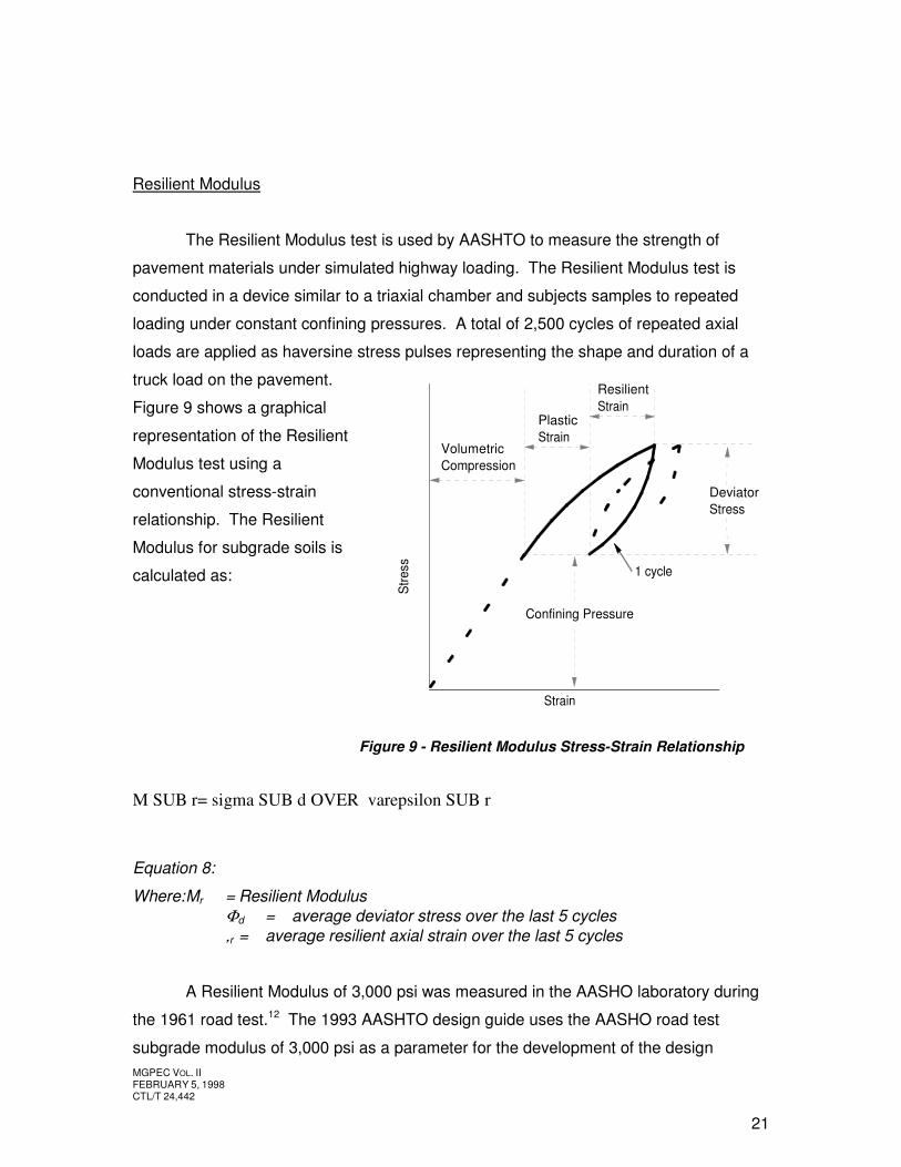
The Resilient Modulus test is used by AASHTO to measure the strength of
pavement materials under simulated highway loading. The Resilient Modulus test is
conducted in a device similar to a triaxial chamber and subjects samples to repeated
loading under constant confining pressures. A total of 2,500 cycles of repeated axial
loads are applied as haversine stress pulses representing the shape and duration of a
truck load on the pavement.
Figure 9 shows a graphical
representation of the Resilient
Modulus test using a
conventional stress-strain
relationship. The Resilient
Modulus for subgrade soils is
calculated as:
Equation 8:
Where: Mr = Resilient Modulus Φd = average deviator stress over the last 5 cycles ,r = average resilient axial strain over the last 5 cycles A Resilient Modulus of 3,000 psi was measured in the AASHO laboratory during
the 1961 road test.12 The 1993 AASHTO design guide uses the AASHO road test
subgrade modulus of 3,000 psi as a parameter for the development of the design
Figure 9 - Resilient Modulus Stress-Strain Relationship
Volumetric Compression
Plastic Strain
Resilient Strain
Deviator Stress
Confining Pressure
Strain
Stre
ss 1 cycle
M SUB r= sigma SUB d OVER varepsilon SUB r

MGPEC VOL. II FEBRUARY 5, 1998 CTL/T 24,442
22
equation. The methods used to measure subgrade modulus have changed significantly
since the AASHO road test. Measured Resilient Modulus values must be adjusted to
provide consistency with the values used in the development of the 1993 design
equation. Thompson and Robnett13 studied the behavior of the AASHO soils and
concluded that a deviator stress of 6 psi and a confining pressure of 0 psi approximated
conditions of the road test, which were used for the 1993 AASHTO design guide. In this
material property study, the subgrade Resilient Modulus was determined using these
stresses on the same forty samples tested in the conventional testing study.
Typical specifications for subgrade compaction require moisture contents at
optimum moisture to 2 percent above optimum. Since no major changes are foreseen in
local specifications, Resilient Modulus testing was conducted at 2 percent above the
optimum moisture content.
Laboratory Resilient Modulus tests were performed using the Colorado
Department of Transportation’s equipment, manufactured by Structural Behavior
Engineering Laboratories and following AASHTO T 294-94 (Strategic Highway Research
Program Protocol P46). Laboratory procedures prevented preparing samples with exact
target moisture contents. Measured Resilient Modulus values were adjusted for
moisture content variations using Equation 9 presented by Li and Selig14 to obtain a 2
percent over optimum moisture content.
MGPEC VOL. II FEBRUARY 5, 1998 CTL/T 24,442
23
Equation 9: % = 0.96 - 0.18(w - w1) + 0.0067 (w - w1)2 Mr = Mr1 / % Where: w = desired moisture content w1 = measured moisture content % = moisture content adjustment factor Mr = Resilient Modulus at desired moisture content (w) Mr1 = measured Resilient Modulus at measured moisture content (w1)
Moisture Content Effects
Moisture variations occur during the life of a pavement system and cause
changes in subgrade support. These variations are dependent on the surface condition
of the pavement system, drainage, water table, season, and type of subgrade. The
moisture content of the subgrade reaches equilibrium generally within 3 to 10 years after
construction. Local experience and applicable CDOT research indicates clay subgrades
are typically constructed at optimum moisture content to 2 percent wet of optimum and
fail near 5 percent over optimum. For design, the industry traditionally has assumed the
subgrade support is a constant regardless of moisture content and is represented by the
design CBR or R-value. A portion of the material property study evaluated the effects of
moisture content change on the subgrade support value. Resilient Modulus also varies
on a seasonal basis depending upon moisture content and temperature.
MGPEC VOL. II FEBRUARY 5, 1998 CTL/T 24,442
24
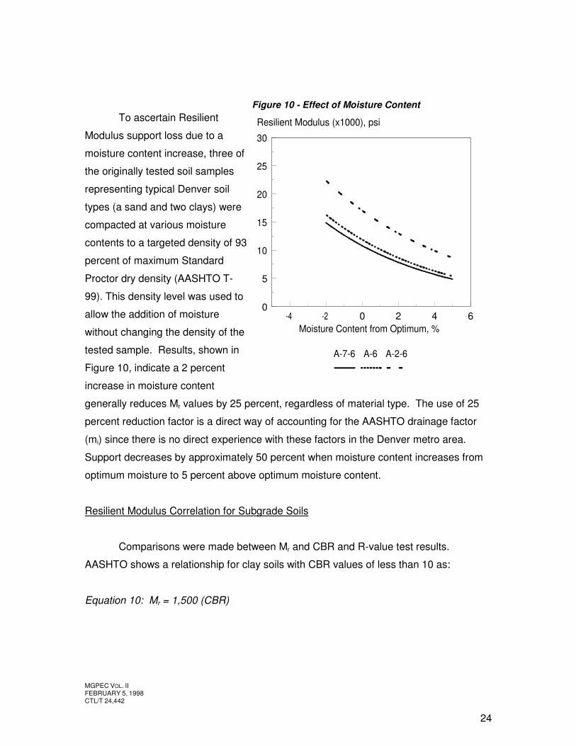
To ascertain Resilient
Modulus support loss due to a
moisture content increase, three of
the originally tested soil samples
representing typical Denver soil
types (a sand and two clays) were
compacted at various moisture
contents to a targeted density of 93
percent of maximum Standard
Proctor dry density (AASHTO T-
99). This density level was used to
allow the addition of moisture
without changing the density of the
tested sample. Results, shown in
Figure 10, indicate a 2 percent
increase in moisture content
generally reduces Mr values by 25 percent, regardless of material type. The use of 25
percent reduction factor is a direct way of accounting for the AASHTO drainage factor
(mi) since there is no direct experience with these factors in the Denver metro area.
Support decreases by approximately 50 percent when moisture content increases from
optimum moisture to 5 percent above optimum moisture content.
Resilient Modulus Correlation for Subgrade Soils
Comparisons were made between Mr and CBR and R-value test results.
AASHTO shows a relationship for clay soils with CBR values of less than 10 as:
Equation 10: Mr = 1,500 (CBR)
Figure 10 - Effect of Moisture Content
-4 -2 0 2 4 60
5
10
15
20
25
30
Moisture Content from Optimum, %
Resilient Modulus (x1000), psi
A-7-6 A-6 A-2-6
MGPEC VOL. II FEBRUARY 5, 1998 CTL/T 24,442
25
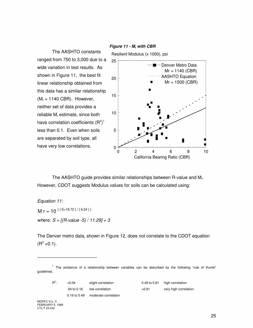
The AASHTO constants
ranged from 750 to 3,000 due to a
wide variation in test results. As
shown in Figure 11, the best fit
linear relationship obtained from
this data has a similar relationship
(Mr = 1140 CBR). However,
neither set of data provides a
reliable Mr estimate, since both
have correlation coefficients (R2)1
less than 0.1. Even when soils
are separated by soil type, all
have very low correlations.
The AASHTO guide provides similar relationships between R-value and Mr.
However, CDOT suggests Modulus values for soils can be calculated using:
Equation 11:
where: S = [(R-value -5) / 11.29] + 3
The Denver metro data, shown in Figure 12, does not correlate to the CDOT equation
(R2 <0.1).
1 The existence of a relationship between variables can be described by the following “rule of thumb” guidelines.
R2: <0.04 slight correlation 0.49 to 0.81 high correlation
.04 to 0.16 low correlation >0.81 very high correlation
0.16 to 0.49 moderate correlation
Figure 11 - Mr with CBR
0 2 4 6 8 100
5
10
15
20
25
California Bearing Ratio (CBR)
Resilient Modulus (x 1000), psi
Denver Metro DataMr = 1140 (CBR)
AASHTO EquationMr = 1500 (CBR)
M r = 10 { { S+18.72 } / { 6.24 } }
MGPEC VOL. II FEBRUARY 5, 1998 CTL/T 24,442
26
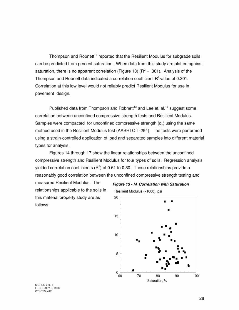
Thompson and Robnett13 reported that the Resilient Modulus for subgrade soils
can be predicted from percent saturation. When data from this study are plotted against
saturation, there is no apparent correlation (Figure 13) (R2 = .301). Analysis of the
Thompson and Robnett data indicated a correlation coefficient R2 value of 0.301.
Correlation at this low level would not reliably predict Resilient Modulus for use in
pavement design.
Published data from Thompson and Robnett13 and Lee et. al.15 suggest some
correlation between unconfined compressive strength tests and Resilient Modulus.
Samples were compacted for unconfined compressive strength (qu) using the same
method used in the Resilient Modulus test (AASHTO T-294). The tests were performed
using a strain-controlled application of load and separated samples into different material
types for analysis.
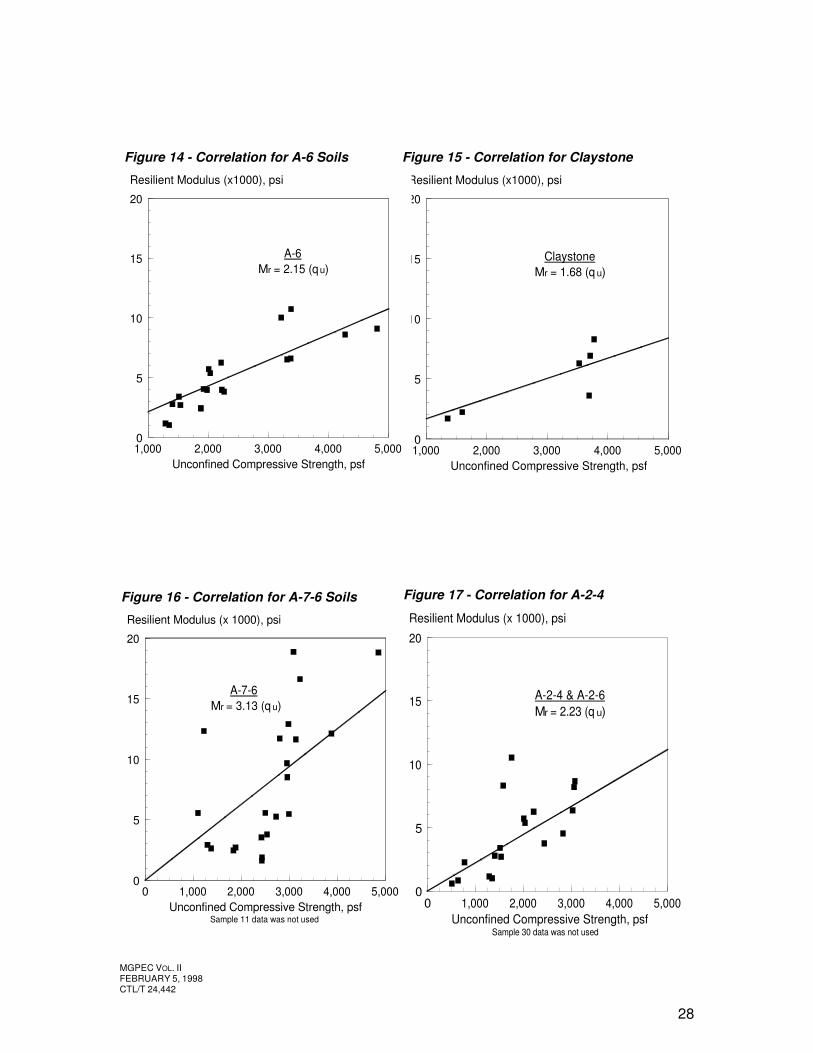
Figures 14 through 17 show the linear relationships between the unconfined
compressive strength and Resilient Modulus for four types of soils. Regression analysis
yielded correlation coefficients (R2) of 0.61 to 0.80. These relationships provide a
reasonably good correlation between the unconfined compressive strength testing and
measured Resilient Modulus. The
relationships applicable to the soils in
this material property study are as
follows:
Figure 13 - Mr Correlation with Saturation
60 70 80 90 1000
5
10
15
20
Saturation, %
Resilient Modulus (x1000), psi
MGPEC VOL. II FEBRUARY 5, 1998 CTL/T 24,442
27
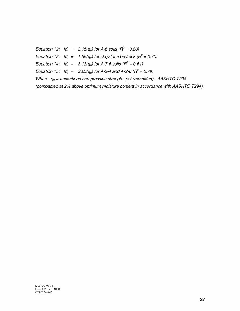
Equation 12: Mr = 2.15(qu) for A-6 soils (R2 = 0.80)
Equation 13: Mr = 1.68(qu) for claystone bedrock (R2 = 0.70)
Equation 14: Mr = 3.13(qu) for A-7-6 soils (R2 = 0.61)
Equation 15: Mr = 2.23(qu) for A-2-4 and A-2-6 (R2 = 0.79)
Where qu = unconfined compressive strength, psf (remolded) - AASHTO T208
(compacted at 2% above optimum moisture content in accordance with AASHTO T294).
MGPEC VOL. II FEBRUARY 5, 1998 CTL/T 24,442
28
Figure 15 - Correlation for Claystone Figure 14 - Correlation for A-6 Soils
Figure 16 - Correlation for A-7-6 Soils Figure 17 - Correlation for A-2-4
and A-2-6 Soils
1,000 2,000 3,000 4,000 5,0000
5
10
15
20
Unconfined Compressive Strength, psf
Resilient Modulus (x1000), psi
ClaystoneMr = 1.68 (q u)
1,000 2,000 3,000 4,000 5,0000
5
10
15
20
Unconfined Compressive Strength, psf
Resilient Modulus (x1000), psi
A-6Mr = 2.15 (q u)
Sample 11 data was not used
0 1,000 2,000 3,000 4,000 5,0000
5
10
15
20
Unconfined Compressive Strength, psf
Resilient Modulus (x 1000), psi
A-7-6Mr = 3.13 (q u)
Sample 30 data was not used
0 1,000 2,000 3,000 4,000 5,0000
5
10
15
20
Unconfined Compressive Strength, psf
Resilient Modulus (x 1000), psi
A-2-4 & A-2-6Mr = 2.23 (q u)
MGPEC VOL. II FEBRUARY 5, 1998 CTL/T 24,442
29
When projects encounter comparatively clean sands, unconfined strength testing
will not be possible. Given the rare occasions when this will occur in Denver, we believe
conventional R-value testing will provide satisfactory estimates of subgrade support.
These R-values should be converted to MR values using Equation 11.
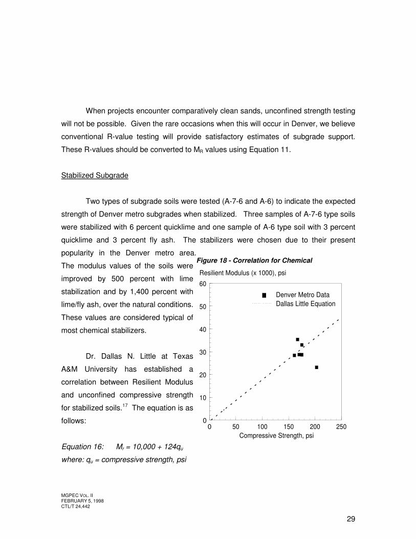
Stabilized Subgrade
Two types of subgrade soils were tested (A-7-6 and A-6) to indicate the expected
strength of Denver metro subgrades when stabilized. Three samples of A-7-6 type soils
were stabilized with 6 percent quicklime and one sample of A-6 type soil with 3 percent
quicklime and 3 percent fly ash. The stabilizers were chosen due to their present
popularity in the Denver metro area.
The modulus values of the soils were
improved by 500 percent with lime
stabilization and by 1,400 percent with
lime/fly ash, over the natural conditions.
These values are considered typical of
most chemical stabilizers.
Dr. Dallas N. Little at Texas
A&M University has established a
correlation between Resilient Modulus
and unconfined compressive strength
for stabilized soils.17 The equation is as
follows:
Equation 16: Mr = 10,000 + 124qu
where: qu = compressive strength, psi
Figure 18 - Correlation for Chemical
Stabilized Subgrades
0 50 100 150 200 2500
10
20
30
40
50
60
Compressive Strength, psi
Resilient Modulus (x 1000), psi
Denver Metro DataDallas Little Equation
MGPEC VOL. II FEBRUARY 5, 1998 CTL/T 24,442
30
The correlation from Equation 16
appears applicable to local data as shown
in Figure 18 and is recommended for use
in design for all chemical stabilizers.
Denver metro data presented in the figure
are duplicate sets of three samples of the
A-7-6 soils.
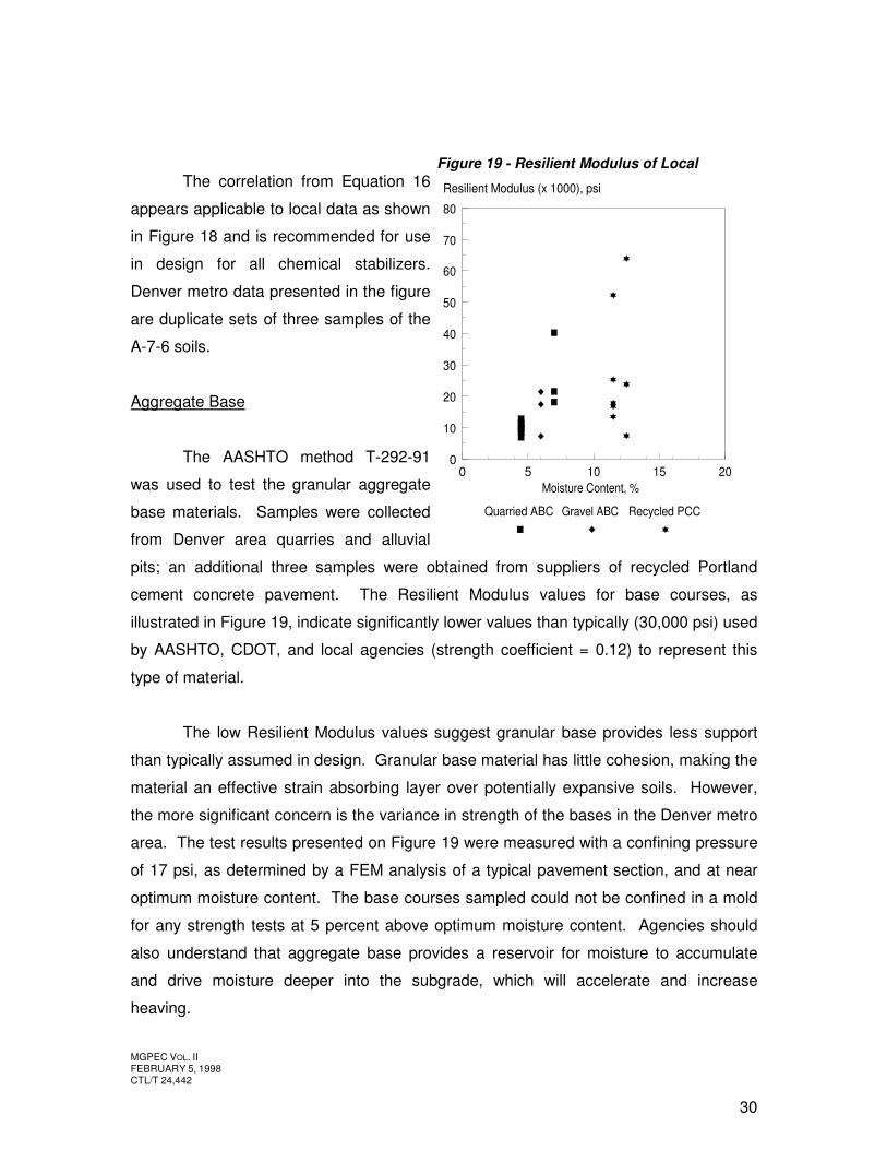
Aggregate Base
The AASHTO method T-292-91
was used to test the granular aggregate
base materials. Samples were collected
from Denver area quarries and alluvial
pits; an additional three samples were obtained from suppliers of recycled Portland
cement concrete pavement. The Resilient Modulus values for base courses, as
illustrated in Figure 19, indicate significantly lower values than typically (30,000 psi) used
by AASHTO, CDOT, and local agencies (strength coefficient = 0.12) to represent this
type of material.
The low Resilient Modulus values suggest granular base provides less support
than typically assumed in design. Granular base material has little cohesion, making the
material an effective strain absorbing layer over potentially expansive soils. However,
the more significant concern is the variance in strength of the bases in the Denver metro
area. The test results presented on Figure 19 were measured with a confining pressure
of 17 psi, as determined by a FEM analysis of a typical pavement section, and at near
optimum moisture content. The base courses sampled could not be confined in a mold
for any strength tests at 5 percent above optimum moisture content. Agencies should
also understand that aggregate base provides a reservoir for moisture to accumulate
and drive moisture deeper into the subgrade, which will accelerate and increase
heaving.
Figure 19 - Resilient Modulus of Local
Aggregate Base Courses
0 5 10 15 200
10
20
30
40
50
60
70
80
Moisture Content, %
Resilient Modulus (x 1000), psi
Quarried ABC Gravel ABC Recycled PCC
MGPEC VOL. II FEBRUARY 5, 1998 CTL/T 24,442
31
Based on the values presented in Figure 19, a minimum Resilient Modulus value
of 20,000 psi was chosen for design purposes. A Resilient Moduli less than 20,000 psi
becomes relatively equivalent as a support layer to typical Denver metro subgrades,
resulting in little benefit of use of a base layer. Typical Denver metro clay subgrades
produce Mr values of 3,000 to 5,000 psi while Denver metro sands provide Mr values of
10,000 to 15,000 psi. This minimum Mr of 20,000 psi was used in the design procedure
to represent typically produced aggregate base course. It is recommended that
aggregate base only be used in residential streets due to the low support value and
potential for loss of support of the aggregate base. This recommendation is based upon
the integrity of the base course regardless of the subgrade type.
Experience has shown aggregate base tends to migrate into a clay subgrade as
the clay also pumps into the aggregate base. In an effort to reduce the migration of clay
fines and base material, a woven, high strength fabric should be utilized as a separation
layer.18 In areas of clay soils, a fabric placed on top of the subgrade, beneath the
aggregate base will help confine the base and reduce the loss of support experienced
with migration.
Asphalt Cement Concrete Pavement
We obtained asphalt cement concrete pavement cores from locations in the
metropolitan area to measure Resilient Modulus values to be used with the design
methodology. Asphalt cement concrete varied in design method and the required
compaction level. All pavements were placed during the 1996 construction season.
Resilient Modulus and Indirect Tensile strength testing were performed by the
Central Federal Lands Highway Division located in Denver, Colorado. Testing was
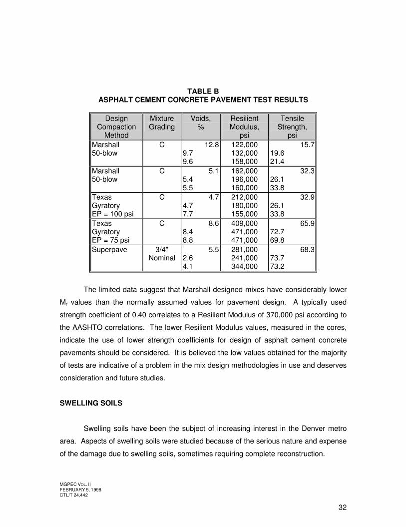
performed at 25ΕC (77ΕF) and results are presented in Table B.
MGPEC VOL. II FEBRUARY 5, 1998 CTL/T 24,442
32
TABLE B
ASPHALT CEMENT CONCRETE PAVEMENT TEST RESULTS
Design Compaction
Method
Mixture Grading
Voids, %
Resilient Modulus,
psi
Tensile Strength,
psi Marshall 50-blow
C 12.8 9.7 9.6
122,000 132,000 158,000
15.7 19.6 21.4
Marshall 50-blow
C 5.1 5.4 5.5
162,000 196,000 160,000
32.3 26.1 33.8
Texas Gyratory EP = 100 psi
C 4.7 4.7 7.7
212,000 180,000 155,000
32.9 26.1 33.8
Texas Gyratory EP = 75 psi
C 8.6 8.4 8.8
409,000 471,000 471,000
65.9 72.7 69.8
Superpave 3/4" Nominal
5.5 2.6 4.1
281,000 241,000 344,000
68.3 73.7 73.2
The limited data suggest that Marshall designed mixes have considerably lower
Mr values than the normally assumed values for pavement design. A typically used
strength coefficient of 0.40 correlates to a Resilient Modulus of 370,000 psi according to
the AASHTO correlations. The lower Resilient Modulus values, measured in the cores,
indicate the use of lower strength coefficients for design of asphalt cement concrete
pavements should be considered. It is believed the low values obtained for the majority
of tests are indicative of a problem in the mix design methodologies in use and deserves
consideration and future studies.
SWELLING SOILS
Swelling soils have been the subject of increasing interest in the Denver metro
area. Aspects of swelling soils were studied because of the serious nature and expense
of the damage due to swelling soils, sometimes requiring complete reconstruction.
MGPEC VOL. II FEBRUARY 5, 1998 CTL/T 24,442
33
Characterization
Classification testing of the soils included measurements of Atterberg Limits and
percent passing the No. 200 sieve (-200). We also measured swell of samples
compacted to about 95 percent of maximum (ASTM D698) dry density at a moisture
content about 2 percent above optimum moisture. Test specimens were confined under
an applied pressure of 200 pounds per square foot (psf) prior to wetting. The measured
swell was compared with sample liquid limit (LL), plasticity index (PI), and optimum
moisture content. The results showed that measured swell increased with increasing LL,
PI, and optimum moisture content.
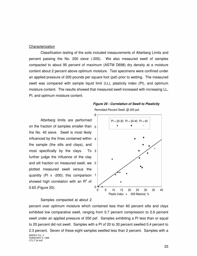
Atterberg limits are performed
on the fraction of samples smaller than
the No. 40 sieve. Swell is most likely
influenced by the fines contained within
the sample (the silts and clays), and
most specifically by the clays. To
further judge the influence of the clay
and silt fraction on measured swell, we
plotted measured swell versus the
quantity (PI x -200); this comparison
showed high correlation with an R2 of
0.63 (Figure 20).
Samples compacted at about 2
percent over optimum moisture which contained less than 60 percent silts and clays
exhibited low comparative swell, ranging from 0.7 percent compression to 2.6 percent
swell under an applied pressure of 200 psf. Samples exhibiting a PI less than or equal
to 20 percent did not swell. Samples with a PI of 20 to 30 percent swelled 0.4 percent to
2.3 percent. Seven of these eight samples swelled less than 2 percent. Samples with a
Figure 20 - Correlation of Swell to Plasticity
Index and Clay Material
0 5 10 15 20 25 30 35 400
1
2
3
4
5
6
Plastic Index x -200 Material, %
Remolded Percent Swell, @ 200 psf.
PI = 20-30 PI = 30-40 PI > 40
MGPEC VOL. II FEBRUARY 5, 1998 CTL/T 24,442
34
PI between 30 and 40 percent swelled 1.6 to 4 percent. Two samples with a PI greater
than 40 percent swelled 3.2 percent.
The data also indicate it is not possible to achieve “zero swell” with moisture
treatment achievable with common construction techniques. Rather, the results
demonstrate that the goal of moisture treatment should be to reduce swell to control
potential differential heave by creating a more uniform material below the pavement and,
to some degree, reduce total heave.
A parametric study was performed using numerical simulation to evaluate the
magnitude of differential surface deformations resulting from heave of soils below a
moisture treated layer. The calculations were also used to simulate the effect of varying
the depth of moisture treated soil, which to some degree reduces heave and provides
some strain absorption. The analyses were conducted using SIGMA/W, a two-
dimensional finite element stress analysis program.10
A 100-foot-long cross section was formulated for this numerical modeling study.
The moisture treated zone was treated as non-expansive, although this is not practically
achievable using compacted swelling materials. Differential displacements at the surface
of the expansive material below the moisture treated zone were calculated based on the
swell of the underlying subgrade soil.
The effect of the moisture treatment in reducing differential heave was calculated
using six different moisture treated thicknesses (2, 4, 6, 8, 10, and 12 feet). The
potential swell of the soils below the moisture treated layer ranged from 2 percent to 12
percent, assuming a depth of wetting of 11 feet. The depth of wetting was based upon
measurements taken at Front Range Airport at the time of construction and again after
more than 15 years of service.16 The swell of the native materials was reduced with
depth to account for the effects of increasing overburden pressure.
With each variation in depth of moisture treatment and swell of the underlying
soils, a maximum deflection was calculated at the surface of the modeled asphalt
MGPEC VOL. II FEBRUARY 5, 1998 CTL/T 24,442
35
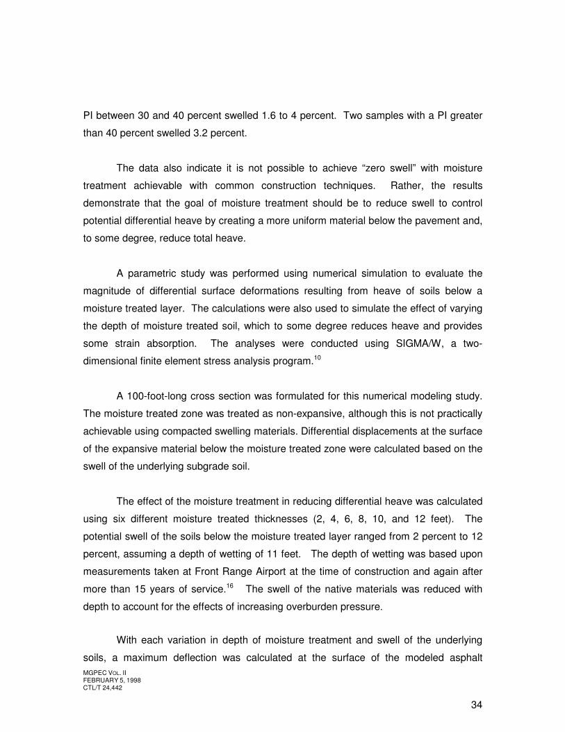
cement concrete pavement layer.
A heave feature in the street was
produced by the model to
represent a bump, perpendicular to
the direction of travel, felt by a
driver. Since the perception of a
bump for a driver is directly related
to the slope of the bump, the slope
of each heave feature was plotted
versus the depth of moisture
treatment (Figure 21).
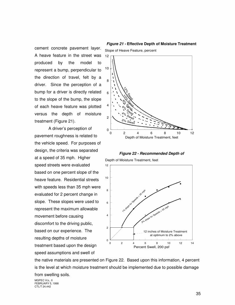
A driver’s perception of
pavement roughness is related to
the vehicle speed. For purposes of
design, the criteria was separated
at a speed of 35 mph. Higher
speed streets were evaluated
based on one percent slope of the
heave feature. Residential streets
with speeds less than 35 mph were
evaluated for 2 percent change in
slope. These slopes were used to
represent the maximum allowable
movement before causing
discomfort to the driving public,
based on our experience. The
resulting depths of moisture
treatment based upon the design
speed assumptions and swell of
the native materials are presented on Figure 22. Based upon this information, 4 percent
is the level at which moisture treatment should be implemented due to possible damage
from swelling soils.
Figure 21 - Effective Depth of Moisture Treatment
Figure 22 - Recommended Depth of
Moisture Treatment
0 2 4 6 8 10 120
2
4
6
8
10
12
Depth of Moisture Treatment, feet
Slope of Heave Feature, percent
12% S
well
10% Sw
ell
8% Swell
6% Swell4% Swell2% Swell
0 2 4 6 8 10 12 140
2
4
6
8
10
12
Percent Swell, 200 psf
Depth of Moisture Treatment, feet
1% sl
ope f
or S
peed
s > 35
mph
2% slope for Speeds < 35 mph
12 inches of Moisture Treatment at optimum to 2% above

MGPEC VOL. II FEBRUARY 5, 1998 CTL/T 24,442
36
Swell Mitigation Recommendations
The results of the analyses performed as part of this investigation indicate a
reduction in heave and differential heave of pavements can be achieved through
moisture treatment of the soils below the pavement. It is not possible to eliminate
heave. The experience of the practitioners involved in this study indicates total heave is
generally not a significant cause of pavement failure and distress. Rather, it is
differential heave which usually results in a rough pavement surface, leading to a shorter
pavement life.
In most cases, a combination of moisture treatment of expansive soils below a
pavement in accordance with Figure 22 and stabilization immediately below the
pavement will significantly enhance the performance of pavements. Extensive sub-
excavation and replacement with low expansion materials has been used in the metro
area. This alternative is generally impractical, expensive, and often with little success.
Without proper drainage, sub-excavation and replacement with non-expansive
permeable soils creates a “bathtub” effect which will trap moisture, forcing the swell
deeper. The subexcavation and replacement techniques should not be used in
residential areas where proper drainage can not be provided.
Moisture treatment of clays should be designed to reduce the swell of materials
within the treated zone. For clays, moisture contents over optimum moisture content will
be required. The data from this study indicate where high plasticity clays and claystone
are present, moisture contents averaging 2 percent above optimum may result in about
2 to 4 percent potential swell of the moisture treated materials under ideal laboratory
conditions. There will be variations in swell of the treated zone. Moisture treatment will
likely produce a yielding subgrade. To provide a stable working platform and add
significant structural capacity to the pavement system, it is believed chemical
stabilization of at least 8 inches of the subgrade is appropriate for sites underlain by
moderate to highly plastic clay subgrade materials. Lime is the preferred material for
stabilization of expansive clays and claystone.17 As a minimum, the percentage of lime
MGPEC VOL. II FEBRUARY 5, 1998 CTL/T 24,442
37
used to stabilize subgrade should produce a soil/lime mixture having the following
properties: 1) pH > 12.3 after mellowing, 2) an unconfined compressive strength of 160
psi or greater, 3) swell less than 1 percent under an applied pressure of 200 psf, and 4)
a plasticity index of less than 10.19 More documentation concerning the strength and
durability of lime stabilization is available. Other chemical stabilizers may be suitable, if
the strength and swell reduction criteria are met and approved by the Agency.
DRAINAGE
The moisture content of the subgrade significantly affects the performance of the
pavement system. Moisture contents of 5 percent over optimum moisture content as
typically found below failed pavements, significantly decrease the modulus of the
subgrade. In the past, the AASHTO design procedures have accounted for drainage
through a drainage coefficient applied to the structural thickness equation. However, the
drainage factor has been on a scale of 0 to 1, unrelated to performance characteristics
and chosen at the discretion of the design engineer. Poor drainage was accounted for
by indirectly reducing the support strength and increasing the pavement thickness
through a factor that did not relate to any measurable loss due to poor drainage. Since
most subgrades are placed at optimum to 2 percent above optimum moisture content,
additional amounts of moisture introduced into the subgrade will reduce the support
strength. The designer should provide a method to control the amount of moisture
entering and draining from the pavement system, or design for the loss of support due to
an increase in moisture.
A method of controlling moisture entering the subgrade is the construction of
interceptor or subsurface drains behind the curb and gutter during street construction.
This method requires routine maintenance to assure effective operation of the drain.
The cost to provide the subsurface drainage system and its maintenance may not justify
its use as a solution.
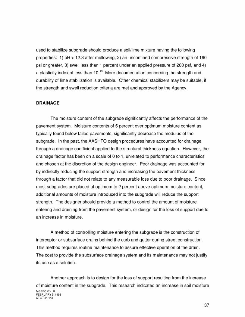
Another approach is to design for the loss of support resulting from the increase
of moisture content in the subgrade. This research indicated an increase in soil moisture
MGPEC VOL. II FEBRUARY 5, 1998 CTL/T 24,442
38
to 5 percent above optimum, from a
constructed moisture content 2
percent above optimum, will reduce
a material’s Resilient Modulus by
approximately 25 percent (Figure
23). Similar conclusions
concerning loss of strength in the
subgrade, due to an increase in
moisture content, have been
documented through other
research.20 In design, the
subgrade Modulus should be
reduced to account for deficiencies
in drainage and the increase in soil
moisture which will occur over time,
especially when irrigation is nearby.
subgrade as the strength is decreased during the pavement service life. Rural
pavements constructed with good surface drainage where moisture is allowed to escape
the subgrade, and no adjacent landscape irrigation will be present, should not have
Resilient Modulus values reduced.
Proper drainage of the pavement system should include the consideration of
drainage characteristics. In rural areas, AASHTO directs the design engineer to design
the road cross-section so that the pavement system can drain into adjacent drainage
ditches. In urban settings, the drainage ditch concept is not possible, reducing the
drainage of the pavement system. In addition, many urban designs include landscaped
medians that must be irrigated, thus adding more moisture into the subgrade. Irrigation
lines within irrigated median can break, causing more damage. During design and
construction of such median features, the amount of irrigation required, drainage of the
median, and the impact of drainage on the pavement system should be considered in
the determination of subgrade support. The medians should be designed to drain into a
Figure 23 - Loss of Subgrade
Resilient Modulus
0 2 50
5
10
15
20
25
10.8
7.8
4.9
11.9
8.6
5.4
17.1
13
8.8
Moisture Content from Optimum, %
Resilient Modulus (x1000), psi
A-7-6 A-6 A-2-6

MGPEC VOL. II FEBRUARY 5, 1998 CTL/T 24,442
39
controlled drainage system to allow for proper plant growth and to protect the pavement
subgrade from loss of support due to an increase in moisture content.
For design, loss of support should be accounted for by providing a drain system
or reduction in the design modulus for any cohesive soils. This restriction does not apply
for free-draining sand soils. Rural pavements often have good surface drainage and
borrow ditches, lower than the pavement surface, where free draining moisture can
escape from the subgrade. Where surface drainage is good and there is no adjacent
landscaping, the modulus reduction is not applicable.
PAVEMENT DESIGN EQUATIONS
The pavement design state-of-practice in the Denver area is the AASHTO design
nomographs as published in 1993. Our literature review indicates that this methodology
is the most common “empirical” method available. “Mechanistic” analysis methods, such
as finite element or elastic layer, require sophisticated computer programs. Even with
these “mechanistic” methods, material property assumptions are required. It is
recommended that agencies should consider “mechanistic” methods in the design of
arterial level streets and other high traffic industrial roadways to improve the accuracy
and reliability of pavement designs.
Flexible Design Sensitivity Analysis
The 1993 AASHTO design equations for both rigid and flexible pavements
serve as the basis of the recommended MGPEC pavement design equations. The
development of the equations included a parametric study of the AASHTO design
variables to assess the sensitivity of the various parameters within the equation. The
AASHTO design method uses five variables in the calculation of a structural number.
These variables include Reliability, Standard Deviation, ESAL20, subgrade Resilient
Modulus, and Loss of Present Serviceability Index (PSI).
A typical range of values was used for each design variable.
MGPEC VOL. II FEBRUARY 5, 1998 CTL/T 24,442
40
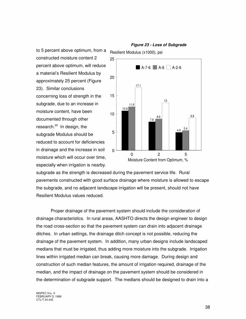
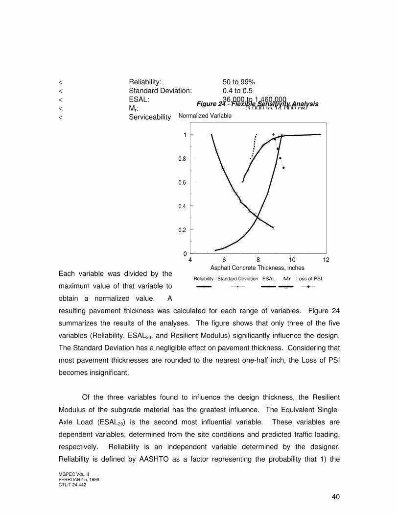
< Reliability: 50 to 99% < Standard Deviation: 0.4 to 0.5 < ESAL: 36,000 to 1,460,000 < Mr: 3,000 to 14,000 psi < Serviceability
Loss:
1.8 to 2.5
Each variable was divided by the
maximum value of that variable to
obtain a normalized value. A
resulting pavement thickness was calculated for each range of variables. Figure 24
summarizes the results of the analyses. The figure shows that only three of the five
variables (Reliability, ESAL20, and Resilient Modulus) significantly influence the design.
The Standard Deviation has a negligible effect on pavement thickness. Considering that
most pavement thicknesses are rounded to the nearest one-half inch, the Loss of PSI
becomes insignificant.
Of the three variables found to influence the design thickness, the Resilient
Modulus of the subgrade material has the greatest influence. The Equivalent Single-
Axle Load (ESAL20) is the second most influential variable. These variables are
dependent variables, determined from the site conditions and predicted traffic loading,
respectively. Reliability is an independent variable determined by the designer.
Reliability is defined by AASHTO as a factor representing the probability that 1) the
Figure 24 - Flexible Sensitivity Analysis
4 6 8 10 120
0.2
0.4
0.6
0.8
1
Asphalt Concrete Thickness, inches
Normalized Variable
Reliability Standard Deviation ESAL Mr Loss of PSI
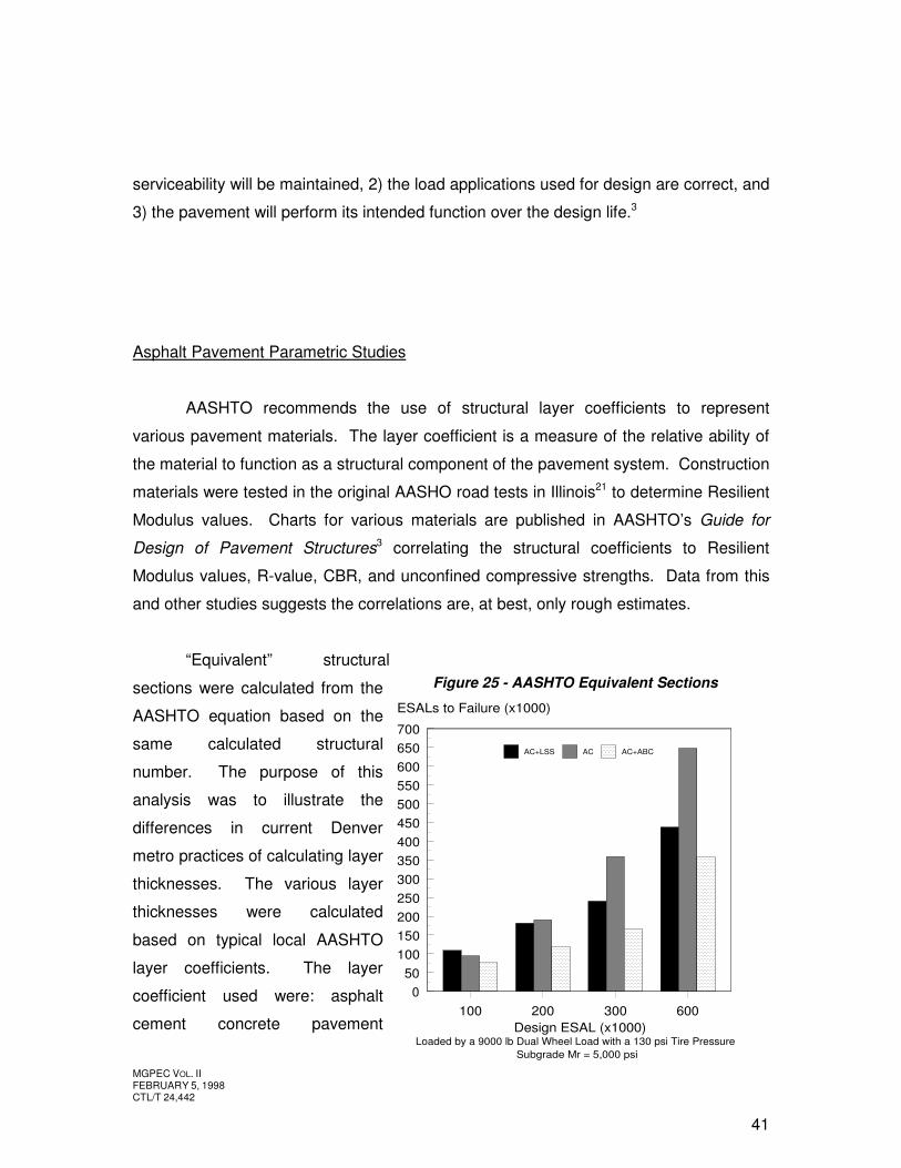
MGPEC VOL. II FEBRUARY 5, 1998 CTL/T 24,442
41
serviceability will be maintained, 2) the load applications used for design are correct, and
3) the pavement will perform its intended function over the design life.3
Asphalt Pavement Parametric Studies
AASHTO recommends the use of structural layer coefficients to represent
various pavement materials. The layer coefficient is a measure of the relative ability of
the material to function as a structural component of the pavement system. Construction
materials were tested in the original AASHO road tests in Illinois21 to determine Resilient
Modulus values. Charts for various materials are published in AASHTO’s Guide for
Design of Pavement Structures3 correlating the structural coefficients to Resilient
Modulus values, R-value, CBR, and unconfined compressive strengths. Data from this
and other studies suggests the correlations are, at best, only rough estimates.
“Equivalent” structural
sections were calculated from the
AASHTO equation based on the
same calculated structural
number. The purpose of this
analysis was to illustrate the
differences in current Denver
metro practices of calculating layer
thicknesses. The various layer
thicknesses were calculated
based on typical local AASHTO
layer coefficients. The layer
coefficient used were: asphalt
cement concrete pavement
Figure 25 - AASHTO Equivalent Sections
Loaded by a 9000 lb Dual Wheel Load with a 130 psi Tire PressureSubgrade Mr = 5,000 psi
100 200 300 6000
50100150200250300350400450500550600650700
Design ESAL (x1000)
ESALs to Failure (x1000)
AC+LSS AC AC+ABC
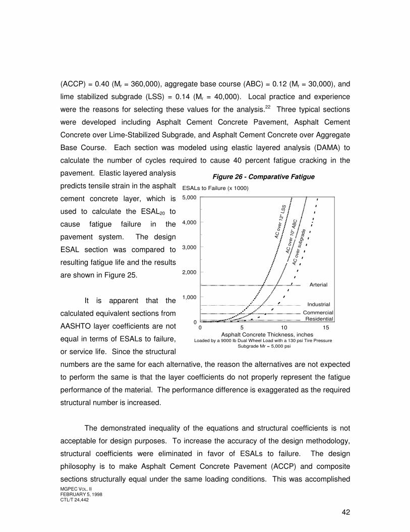
MGPEC VOL. II FEBRUARY 5, 1998 CTL/T 24,442
42
(ACCP) = 0.40 (Mr = 360,000), aggregate base course (ABC) = 0.12 (Mr = 30,000), and
lime stabilized subgrade (LSS) = 0.14 (Mr = 40,000). Local practice and experience
were the reasons for selecting these values for the analysis.22 Three typical sections
were developed including Asphalt Cement Concrete Pavement, Asphalt Cement
Concrete over Lime-Stabilized Subgrade, and Asphalt Cement Concrete over Aggregate
Base Course. Each section was modeled using elastic layered analysis (DAMA) to
calculate the number of cycles required to cause 40 percent fatigue cracking in the
pavement. Elastic layered analysis
predicts tensile strain in the asphalt
cement concrete layer, which is
used to calculate the ESAL20 to
cause fatigue failure in the
pavement system. The design
ESAL section was compared to
resulting fatigue life and the results
are shown in Figure 25.
It is apparent that the
calculated equivalent sections from
AASHTO layer coefficients are not
equal in terms of ESALs to failure,
or service life. Since the structural
numbers are the same for each alternative, the reason the alternatives are not expected
to perform the same is that the layer coefficients do not properly represent the fatigue
performance of the material. The performance difference is exaggerated as the required
structural number is increased.
The demonstrated inequality of the equations and structural coefficients is not
acceptable for design purposes. To increase the accuracy of the design methodology,
structural coefficients were eliminated in favor of ESALs to failure. The design
philosophy is to make Asphalt Cement Concrete Pavement (ACCP) and composite
sections structurally equal under the same loading conditions. This was accomplished
Figure 26 - Comparative Fatigue
Loaded by a 9000 lb Dual Wheel Load with a 130 psi Tire PressureSubgrade Mr = 5,000 psi
0 5 10 150
1,000
2,000
3,000
4,000
5,000
Asphalt Concrete Thickness, inches
ESALs to Failure (x 1000)
AC
ove
r 12"
LS
S
AC
ove
r sub
grad
e
ResidentialCommercial
Industrial
ArterialA
C o
ver 1
0" A
BC
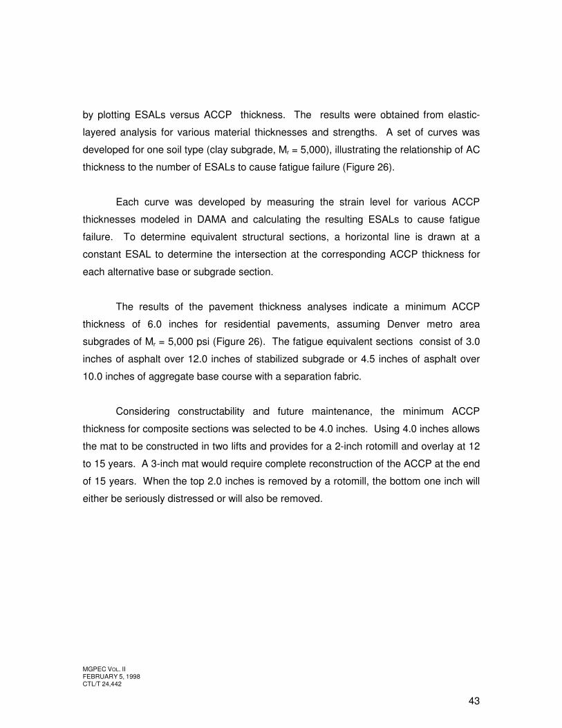
MGPEC VOL. II FEBRUARY 5, 1998 CTL/T 24,442
43
by plotting ESALs versus ACCP thickness. The results were obtained from elastic-
layered analysis for various material thicknesses and strengths. A set of curves was
developed for one soil type (clay subgrade, Mr = 5,000), illustrating the relationship of AC
thickness to the number of ESALs to cause fatigue failure (Figure 26).
Each curve was developed by measuring the strain level for various ACCP
thicknesses modeled in DAMA and calculating the resulting ESALs to cause fatigue
failure. To determine equivalent structural sections, a horizontal line is drawn at a
constant ESAL to determine the intersection at the corresponding ACCP thickness for
each alternative base or subgrade section.
The results of the pavement thickness analyses indicate a minimum ACCP
thickness of 6.0 inches for residential pavements, assuming Denver metro area
subgrades of Mr = 5,000 psi (Figure 26). The fatigue equivalent sections consist of 3.0
inches of asphalt over 12.0 inches of stabilized subgrade or 4.5 inches of asphalt over
10.0 inches of aggregate base course with a separation fabric.
Considering constructability and future maintenance, the minimum ACCP
thickness for composite sections was selected to be 4.0 inches. Using 4.0 inches allows
the mat to be constructed in two lifts and provides for a 2-inch rotomill and overlay at 12
to 15 years. A 3-inch mat would require complete reconstruction of the ACCP at the end
of 15 years. When the top 2.0 inches is removed by a rotomill, the bottom one inch will
either be seriously distressed or will also be removed.
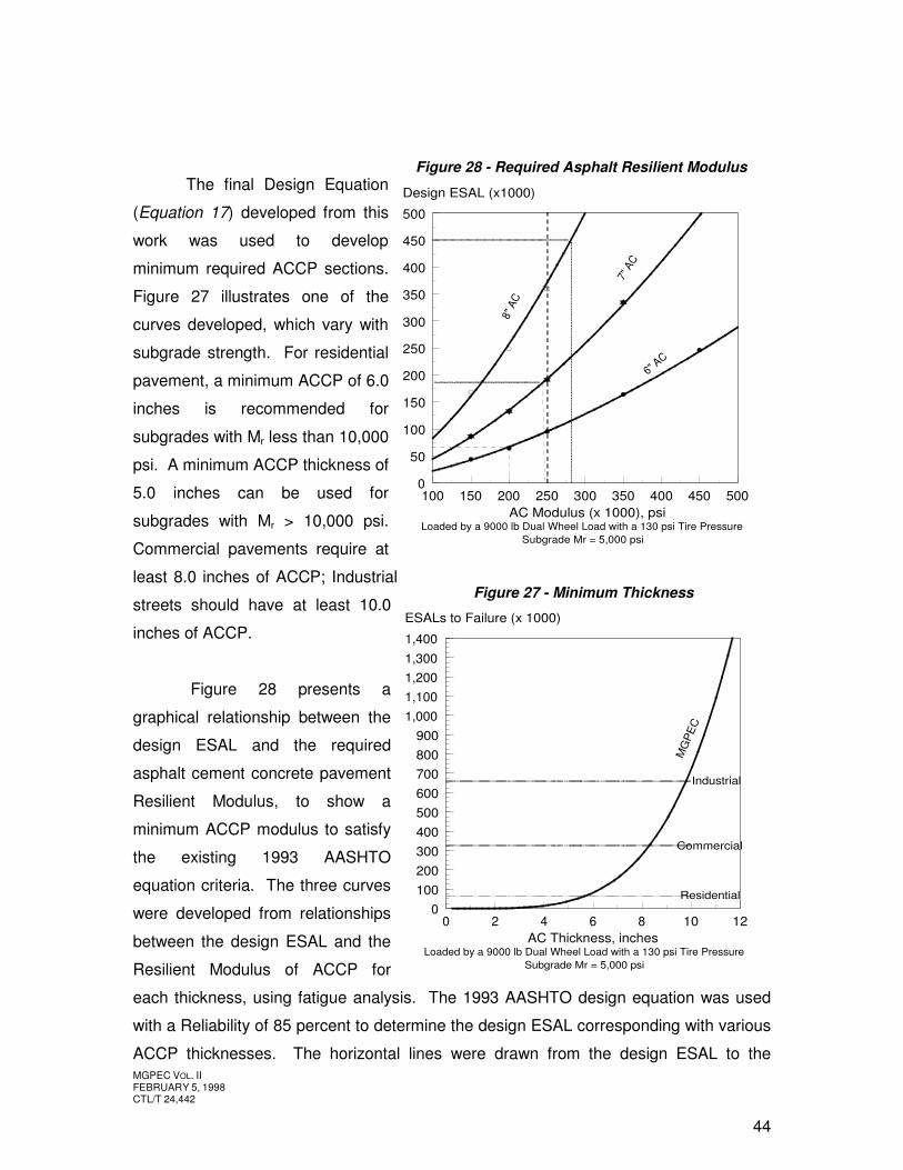
MGPEC VOL. II FEBRUARY 5, 1998 CTL/T 24,442
44
The final Design Equation
(Equation 17) developed from this
work was used to develop
minimum required ACCP sections.
Figure 27 illustrates one of the
curves developed, which vary with
subgrade strength. For residential
pavement, a minimum ACCP of 6.0
inches is recommended for
subgrades with Mr less than 10,000
psi. A minimum ACCP thickness of
5.0 inches can be used for
subgrades with Mr > 10,000 psi.
Commercial pavements require at
least 8.0 inches of ACCP; Industrial
streets should have at least 10.0
inches of ACCP.
Figure 28 presents a
graphical relationship between the
design ESAL and the required
asphalt cement concrete pavement
Resilient Modulus, to show a
minimum ACCP modulus to satisfy
the existing 1993 AASHTO
equation criteria. The three curves
were developed from relationships
between the design ESAL and the
Resilient Modulus of ACCP for
each thickness, using fatigue analysis. The 1993 AASHTO design equation was used
with a Reliability of 85 percent to determine the design ESAL corresponding with various
ACCP thicknesses. The horizontal lines were drawn from the design ESAL to the
Figure 27 - Minimum Thickness
Figure 28 - Required Asphalt Resilient Modulus
Loaded by a 9000 lb Dual Wheel Load with a 130 psi Tire PressureSubgrade Mr = 5,000 psi
0 2 4 6 8 10 120
100200300400500600700800900
1,0001,1001,2001,3001,400
AC Thickness, inches
ESALs to Failure (x 1000)
Residential
Commercial
Industrial
MG
PE
C
Loaded by a 9000 lb Dual Wheel Load with a 130 psi Tire PressureSubgrade Mr = 5,000 psi
100 150 200 250 300 350 400 450 5000
50
100
150
200
250
300
350
400
450
500
AC Modulus (x 1000), psi
Design ESAL (x1000)
7" A
C
6" AC
8" A
C
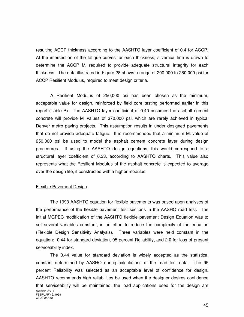
MGPEC VOL. II FEBRUARY 5, 1998 CTL/T 24,442
45
resulting ACCP thickness according to the AASHTO layer coefficient of 0.4 for ACCP.
At the intersection of the fatigue curves for each thickness, a vertical line is drawn to
determine the ACCP Mr required to provide adequate structural integrity for each
thickness. The data illustrated in Figure 28 shows a range of 200,000 to 280,000 psi for
ACCP Resilient Modulus, required to meet design criteria.
A Resilient Modulus of 250,000 psi has been chosen as the minimum,
acceptable value for design, reinforced by field core testing performed earlier in this
report (Table B). The AASHTO layer coefficient of 0.40 assumes the asphalt cement
concrete will provide Mr values of 370,000 psi, which are rarely achieved in typical
Denver metro paving projects. This assumption results in under designed pavements
that do not provide adequate fatigue. It is recommended that a minimum Mr value of
250,000 psi be used to model the asphalt cement concrete layer during design
procedures. If using the AASHTO design equations, this would correspond to a
structural layer coefficient of 0.33, according to AASHTO charts. This value also
represents what the Resilient Modulus of the asphalt concrete is expected to average
over the design life, if constructed with a higher modulus.
Flexible Pavement Design
The 1993 AASHTO equation for flexible pavements was based upon analyses of
the performance of the flexible pavement test sections in the AASHO road test. The
initial MGPEC modification of the AASHTO flexible pavement Design Equation was to
set several variables constant, in an effort to reduce the complexity of the equation
(Flexible Design Sensitivity Analysis). Three variables were held constant in the
equation: 0.44 for standard deviation, 95 percent Reliability, and 2.0 for loss of present
serviceability index.
The 0.44 value for standard deviation is widely accepted as the statistical
constant determined by AASHO during calculations of the road test data. The 95
percent Reliability was selected as an acceptable level of confidence for design.
AASHTO recommends high reliabilities be used when the designer desires confidence
that serviceability will be maintained, the load applications used for the design are
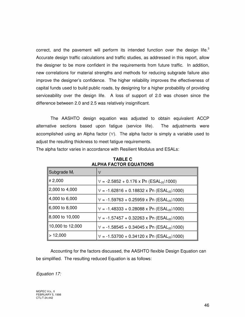
MGPEC VOL. II FEBRUARY 5, 1998 CTL/T 24,442
46
correct, and the pavement will perform its intended function over the design life.3
Accurate design traffic calculations and traffic studies, as addressed in this report, allow
the designer to be more confident in the requirements from future traffic. In addition,
new correlations for material strengths and methods for reducing subgrade failure also
improve the designer’s confidence. The higher reliability improves the effectiveness of
capital funds used to build public roads, by designing for a higher probability of providing
serviceability over the design life. A loss of support of 2.0 was chosen since the
difference between 2.0 and 2.5 was relatively insignificant.
The AASHTO design equation was adjusted to obtain equivalent ACCP
alternative sections based upon fatigue (service life). The adjustments were
accomplished using an Alpha factor (∀). The alpha factor is simply a variable used to
adjust the resulting thickness to meet fatigue requirements.
The alpha factor varies in accordance with Resilient Modulus and ESALs: TABLE C ALPHA FACTOR EQUATIONS
Subgrade Mr ∀
# 2,000 ∀ = -2.5852 + 0.176 x Ρn (ESAL20\1000)
2,000 to 4,000 ∀ = -1.62816 + 0.18832 x Ρn (ESAL20\1000)
4,000 to 6,000 ∀ = -1.59763 + 0.25959 x Ρn (ESAL20\1000)
6,000 to 8,000 ∀ = -1.48333 + 0.28088 x Ρn (ESAL20\1000)
8,000 to 10,000 ∀ = -1.57457 + 0.32263 x Ρn (ESAL20\1000)
10,000 to 12,000 ∀ = -1.58545 + 0.34045 x Ρn (ESAL20\1000)
> 12,000 ∀ = -1.53700 + 0.34120 x Ρn (ESAL20\1000)
Accounting for the factors discussed, the AASHTO flexible Design Equation can
be simplified. The resulting reduced Equation is as follows:
Equation 17:
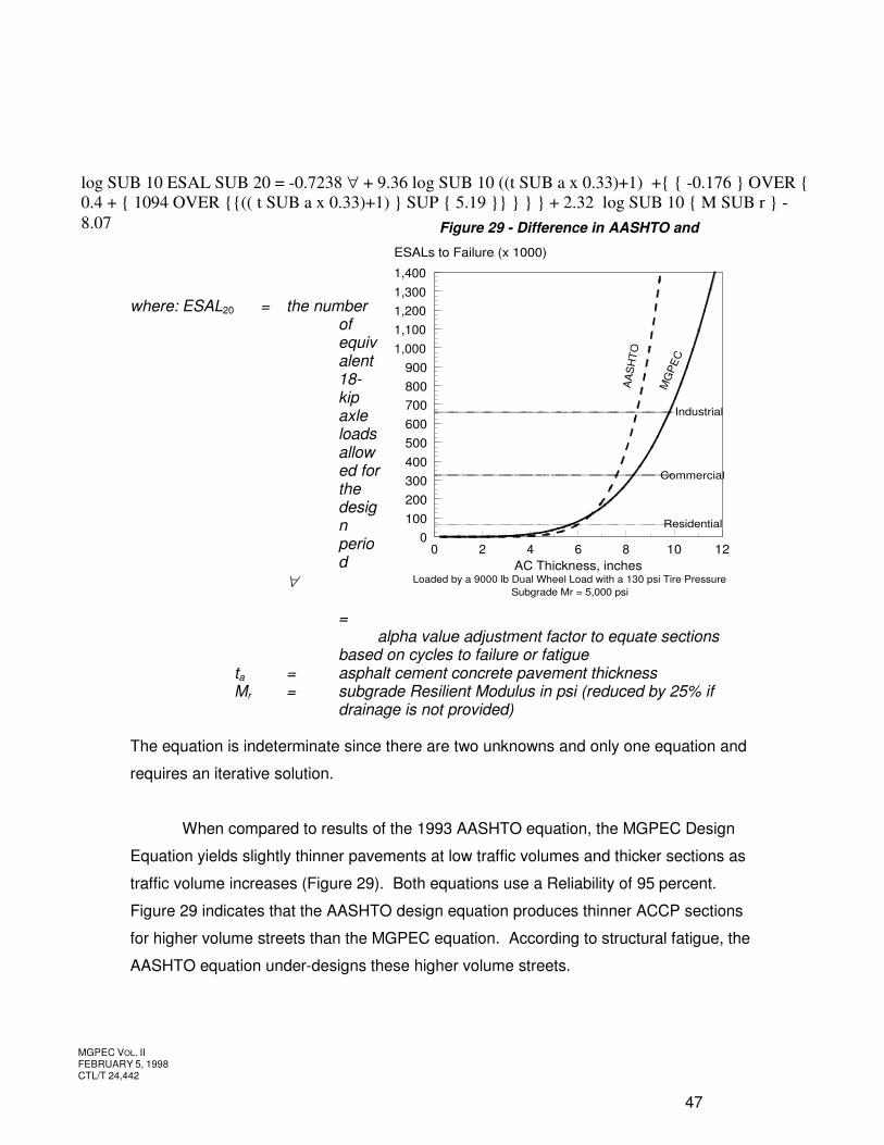
MGPEC VOL. II FEBRUARY 5, 1998 CTL/T 24,442
47
where: ESAL20 = the number of equivalent 18-kip axle loads allowed for the design period
∀ = alpha value adjustment factor to equate sections based on cycles to failure or fatigue
ta = asphalt cement concrete pavement thickness Mr = subgrade Resilient Modulus in psi (reduced by 25% if
drainage is not provided) The equation is indeterminate since there are two unknowns and only one equation and
requires an iterative solution.
When compared to results of the 1993 AASHTO equation, the MGPEC Design
Equation yields slightly thinner pavements at low traffic volumes and thicker sections as
traffic volume increases (Figure 29). Both equations use a Reliability of 95 percent.
Figure 29 indicates that the AASHTO design equation produces thinner ACCP sections
for higher volume streets than the MGPEC equation. According to structural fatigue, the
AASHTO equation under-designs these higher volume streets.
Figure 29 - Difference in AASHTO and
MGPEC Equations
log SUB 10 ESAL SUB 20 = -0.7238 ∀ + 9.36 log SUB 10 ((t SUB a x 0.33)+1) +{ { -0.176 } OVER { 0.4 + { 1094 OVER {{(( t SUB a x 0.33)+1) } SUP { 5.19 }} } } } + 2.32 log SUB 10 { M SUB r } - 8.07
Loaded by a 9000 lb Dual Wheel Load with a 130 psi Tire PressureSubgrade Mr = 5,000 psi
0 2 4 6 8 10 120
100200300400500600700800900
1,0001,1001,2001,3001,400
AC Thickness, inches
ESALs to Failure (x 1000)
Residential
Commercial
Industrial
MG
PE
C
AA
SH
TO
MGPEC VOL. II FEBRUARY 5, 1998 CTL/T 24,442
48
After determining the ACCP thickness, it is recommended that the fatigue criteria
be used as a means of making composite sections “equivalent.” This correlates more
closely to the original intent of the AASHO Committee on Design, by comparing sections
directly by strain levels in the asphalt cement concrete pavement rather than choosing
structural layer values that may not correlate to any measurable physical characteristic
of Denver metro soils. These relationships are illustrated by fatigue curves shown in
Figure 26.
Rigid Design Sensitivity Analysis
The AASHTO design method for rigid pavements, often referred to as Portland
Cement Concrete Pavements (PCCP), uses nine variables for the design of a pavement
section. These variables include concrete Elastic Modulus, concrete Modulus of
Rupture, Load Transfer, Drainage Factor, Reliability, Standard Deviation, ESAL20,
Subgrade Reaction (k), and Loss of Present Serviceability Index. The original AASHO
road test provided the basis for the rigid pavement design equation. Numerous
modifications have been made to create the existing 1993 AASHTO equation.
A rigid design sensitivity analysis was performed using the AASHTO design
variables for rigid pavements, to evaluate their importance and influence on the resulting
pavement thickness and to determine which variables should be used in the design
equation.
< Serviceability Loss: 1.5 to 3.0 < Subgrade Reaction: 40 to 320 pci < Reliability: 60 to
99% < Standard Deviation: 0.2 to 0.45 < Elastic Modulus: 2.5 x 10⁶ to 7
x 106 psi < Modulus of Rupture: 550 to 800 psi < Load Transfer: 2.0 to 5.0 < Drainage: 0.7 to
1.2 < ESAL: 36,500 to
3,650,000
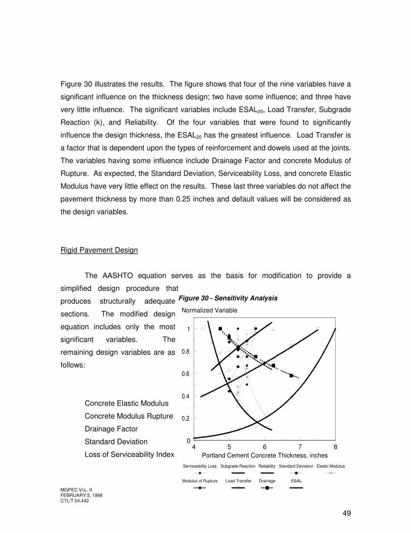
MGPEC VOL. II FEBRUARY 5, 1998 CTL/T 24,442
49
Figure 30 illustrates the results. The figure shows that four of the nine variables have a
significant influence on the thickness design; two have some influence; and three have
very little influence. The significant variables include ESAL20, Load Transfer, Subgrade
Reaction (k), and Reliability. Of the four variables that were found to significantly
influence the design thickness, the ESAL20 has the greatest influence. Load Transfer is
a factor that is dependent upon the types of reinforcement and dowels used at the joints.
The variables having some influence include Drainage Factor and concrete Modulus of
Rupture. As expected, the Standard Deviation, Serviceability Loss, and concrete Elastic
Modulus have very little effect on the results. These last three variables do not affect the
pavement thickness by more than 0.25 inches and default values will be considered as
the design variables.
Rigid Pavement Design
The AASHTO equation serves as the basis for modification to provide a
simplified design procedure that
produces structurally adequate
sections. The modified design
equation includes only the most
significant variables. The
remaining design variables are as
follows:
Concrete Elastic Modulus = 3,400,000 psi
Concrete Modulus Rupture = 650 psi
Drainage Factor = 1.0
Standard Deviation = 0.34
Loss of Serviceability Index = 2.0
Figure 30 - Sensitivity Analysis
4 5 6 7 80
0.2
0.4
0.6
0.8
1
Portland Cement Concrete Thickness, inches
Normalized Variable
Serviceability Loss Subgrade Reaction Reliability Standard Deviation Elastic Modulus
Modulus of Rupture Load Transfer Drainage ESAL
MGPEC VOL. II FEBRUARY 5, 1998 CTL/T 24,442
50
Concrete strength values are commonly specified levels that are typically held
constant in the current design procedures. A Drainage Factor of 1.0 is typical. Drainage
is accounted for in the calculation of the Resilient Modulus and the resulting Modulus of
Subgrade Reaction. The Standard Deviation and Loss of Serviceability Index are typical
design variables that have very little influence on the design thickness.
The design ESALs for use in the rigid pavement design are based upon the
calculations presented earlier in this report using flexible Load Equivalency Factors.
AASHTO provided different Load Equivalency Factors for flexible and rigid pavements to
account for different performance of the two pavement types. The alpha factor used in
the ACCP design equation, serves to distinguish between expected performance of the
ACCP and PCCP design sections. Furthermore, most Denver metro jurisdictions
currently use the same ESAL for both pavement types. It is recommended that the
same ESAL be used for rigid pavements as calculated for flexible pavement sections.
The resulting equation is as follows:
Equation 18:
Where: ESAL20 = the number of equivalent 18-kip axle loads allowed for the design
period tp = Portland cement concrete pavement
thickness required for the pavement system J = load transfer coefficient k = modulus of subgrade reaction. where: k = 0.8932 (Mr / 19.4)(0.827)
log SUB 10 ESAL SUB 20 = -0.5624 + 7.35 log SUB 10 (t SUB p+1) - 0.06 + { { -0.176 } OVER { 1+ { { 1.6248*{10 SUP { 7 } } } } OVER { (t SUB p+1) SUP { 8.46 } } } }+ 3.42 log SUB { 10 } { {650 { ({ t SUP {0.75 } } - 1.132 )} } OVER { 215.63 x J [ { {( t SUB p SUP { 0.75 } ) } - { { 18.42 } OVER { { ({ 3,400,000 } OVER k )} SUP { 0.25 } } } } ]} }
MGPEC VOL. II FEBRUARY 5, 1998 CTL/T 24,442
51
The equation must be solved through an iterative solution to calculate the PCCP
thickness (tp). Portland cement concrete pavements are recommended on sand
subgrades classified as A-1, A-2-4, A-2-5, A-3, A-4, or A-5 by AASHTO classification
procedures. AASHTO provides equations for determining modulus of subgrade reaction
based on Resilient Modulus, as shown above.
In the Denver metro area, the majority of performance problems related to PCCP
are a direct result of swelling soils causing differential movement. In areas where PCCP
has been placed on non-swelling soils, the pavements have performed very well. PCCP
provides a very durable platform with relatively low maintenance requirements when
compared to ACCP. Areas of heavy truck traffic also perform much better when paved
with PCCP, which do not experience the shoving and rutting often experienced with ACC
pavements.
The main concern with the application of a PCCP is the preparation of the
subgrade. PCCP are not recommended for use in areas of greater than 4 percent swell.
If they are used, the subgrade should be stabilized to reduce the effect of heave
damage. Even with stabilization, damage often occurs because of improper drainage of
the subgrade. Asphalt Cement Concrete Pavements are flexible and tend to allow small
amounts of swell without experiencing cracking. If swelling does occur in the subgrade,
ACCP often provide a smoother ride than PCCP and are easier and cheaper to repave
in isolated areas.
Design of Arterial Roadways
The variability associated with arterial roadways does not lend itself to simplistic
design methods. The recommended design process begins with the traffic study and the
lane-by-lane breakdown of volumes.
MGPEC VOL. II FEBRUARY 5, 1998 CTL/T 24,442
52
Pavement alternatives from the MGPEC design equations should consider
thickness ratios for stabilized subgrade/asphalt cement concrete pavement thickness, in
the range of 2 to 3 to properly distribute stresses. Use of aggregate bases beneath
arterial pavements is not recommended as part of the structural section. Rigid (PCCP)
pavements should not be used in areas where treated or untreated subgrade soil swell
potential is greater than 4.0 percent, according to swell potential damage levels
discussed in SWELLING SOILS.
Once preliminary designs have been established and rational thicknesses
obtained, at least three design alternatives, generally consisting of asphalt cement
concrete pavement, asphalt cement concrete pavement over stabilized subgrade, and
Portland cement concrete pavement should be evaluated. The MGPEC equations may
provide sections that could be deficient in thickness according to fatigue life for traffic
volumes over 1,500,000 ESALs. The evaluation should consist of analysis using finite
element or elastic layer techniques to verify ESALs to failure for each of the alternatives
on a lane-by-lane basis. The DAMA program is recommended as one of the best
programs because it analyzes most correctly the maximum surface deflection, tensile
strain at the bottom of the asphalt layer, and compressive strain at the top of the
subgrade.6 Those sections which fail to exceed the design ESALs should either be
adjusted or removed from consideration. After preliminary design, each alternative
should be subjected to life-cycle cost analysis to determine the best present worth
section for each travel lane to be paved.
The pavement design for arterial streets should also include recommendations
for pavement maintenance that consider the user cost associated with lane closures and
delays. The surface course, whether asphalt cement concrete pavement or Portland
cement concrete pavement, should be designed to minimize maintenance through use
of treatments that will ensure the highest practical level of service and the least user
cost.
PAVEMENT MAINTENANCE
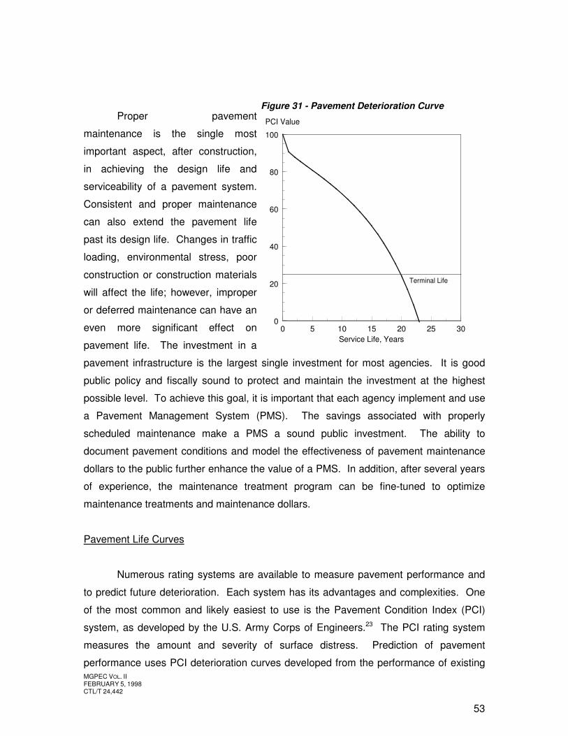
MGPEC VOL. II FEBRUARY 5, 1998 CTL/T 24,442
53
Proper pavement
maintenance is the single most
important aspect, after construction,
in achieving the design life and
serviceability of a pavement system.
Consistent and proper maintenance
can also extend the pavement life
past its design life. Changes in traffic
loading, environmental stress, poor
construction or construction materials
will affect the life; however, improper
or deferred maintenance can have an
even more significant effect on
pavement life. The investment in a
pavement infrastructure is the largest single investment for most agencies. It is good
public policy and fiscally sound to protect and maintain the investment at the highest
possible level. To achieve this goal, it is important that each agency implement and use
a Pavement Management System (PMS). The savings associated with properly
scheduled maintenance make a PMS a sound public investment. The ability to
document pavement conditions and model the effectiveness of pavement maintenance
dollars to the public further enhance the value of a PMS. In addition, after several years
of experience, the maintenance treatment program can be fine-tuned to optimize
maintenance treatments and maintenance dollars.
Pavement Life Curves
Numerous rating systems are available to measure pavement performance and
to predict future deterioration. Each system has its advantages and complexities. One
of the most common and likely easiest to use is the Pavement Condition Index (PCI)
system, as developed by the U.S. Army Corps of Engineers.23 The PCI rating system
measures the amount and severity of surface distress. Prediction of pavement
performance uses PCI deterioration curves developed from the performance of existing
Figure 31 - Pavement Deterioration Curve
0 5 10 15 20 25 300
20
40
60
80
100
Service Life, Years
PCI Value
Terminal Life
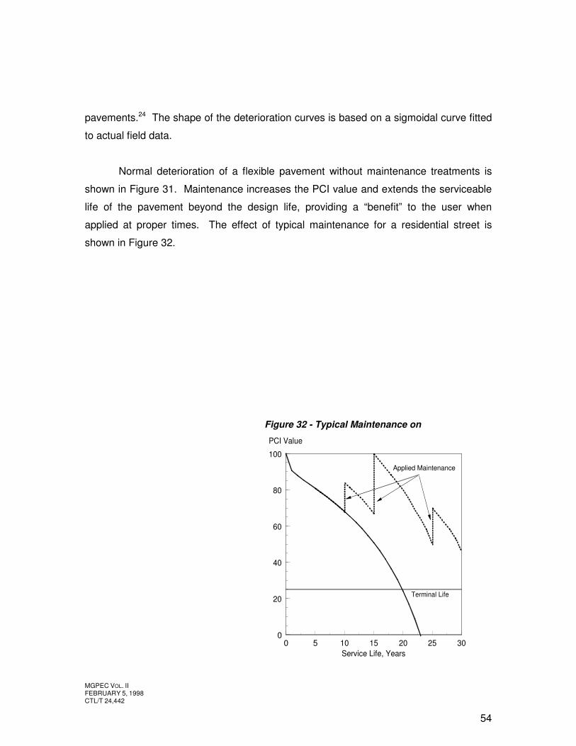
MGPEC VOL. II FEBRUARY 5, 1998 CTL/T 24,442
54
pavements.24 The shape of the deterioration curves is based on a sigmoidal curve fitted
to actual field data.
Normal deterioration of a flexible pavement without maintenance treatments is
shown in Figure 31. Maintenance increases the PCI value and extends the serviceable
life of the pavement beyond the design life, providing a “benefit” to the user when
applied at proper times. The effect of typical maintenance for a residential street is
shown in Figure 32.
Figure 32 - Typical Maintenance on
Residential Streets
0 5 10 15 20 25 300
20
40
60
80
100
Service Life, Years
PCI Value
Terminal Life
Applied Maintenance
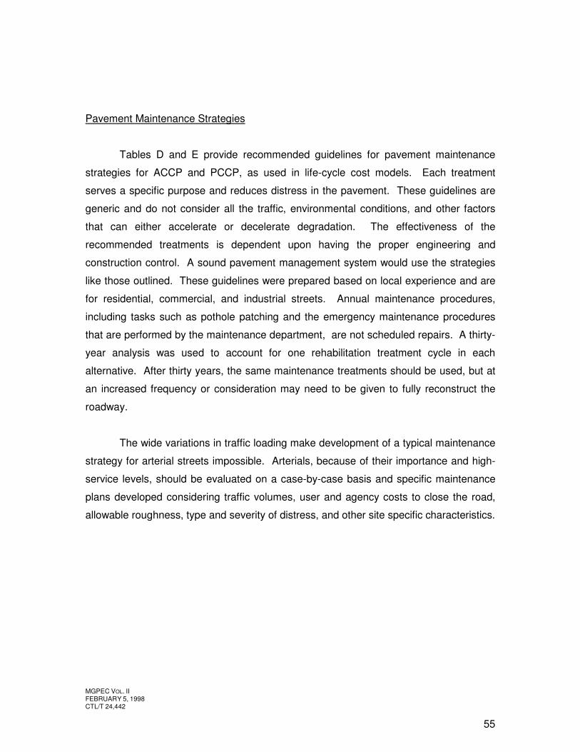
MGPEC VOL. II FEBRUARY 5, 1998 CTL/T 24,442
55
Pavement Maintenance Strategies
Tables D and E provide recommended guidelines for pavement maintenance
strategies for ACCP and PCCP, as used in life-cycle cost models. Each treatment
serves a specific purpose and reduces distress in the pavement. These guidelines are
generic and do not consider all the traffic, environmental conditions, and other factors
that can either accelerate or decelerate degradation. The effectiveness of the
recommended treatments is dependent upon having the proper engineering and
construction control. A sound pavement management system would use the strategies
like those outlined. These guidelines were prepared based on local experience and are
for residential, commercial, and industrial streets. Annual maintenance procedures,
including tasks such as pothole patching and the emergency maintenance procedures
that are performed by the maintenance department, are not scheduled repairs. A thirty-
year analysis was used to account for one rehabilitation treatment cycle in each
alternative. After thirty years, the same maintenance treatments should be used, but at
an increased frequency or consideration may need to be given to fully reconstruct the
roadway.
The wide variations in traffic loading make development of a typical maintenance
strategy for arterial streets impossible. Arterials, because of their importance and high-
service levels, should be evaluated on a case-by-case basis and specific maintenance
plans developed considering traffic volumes, user and agency costs to close the road,
allowable roughness, type and severity of distress, and other site specific characteristics.
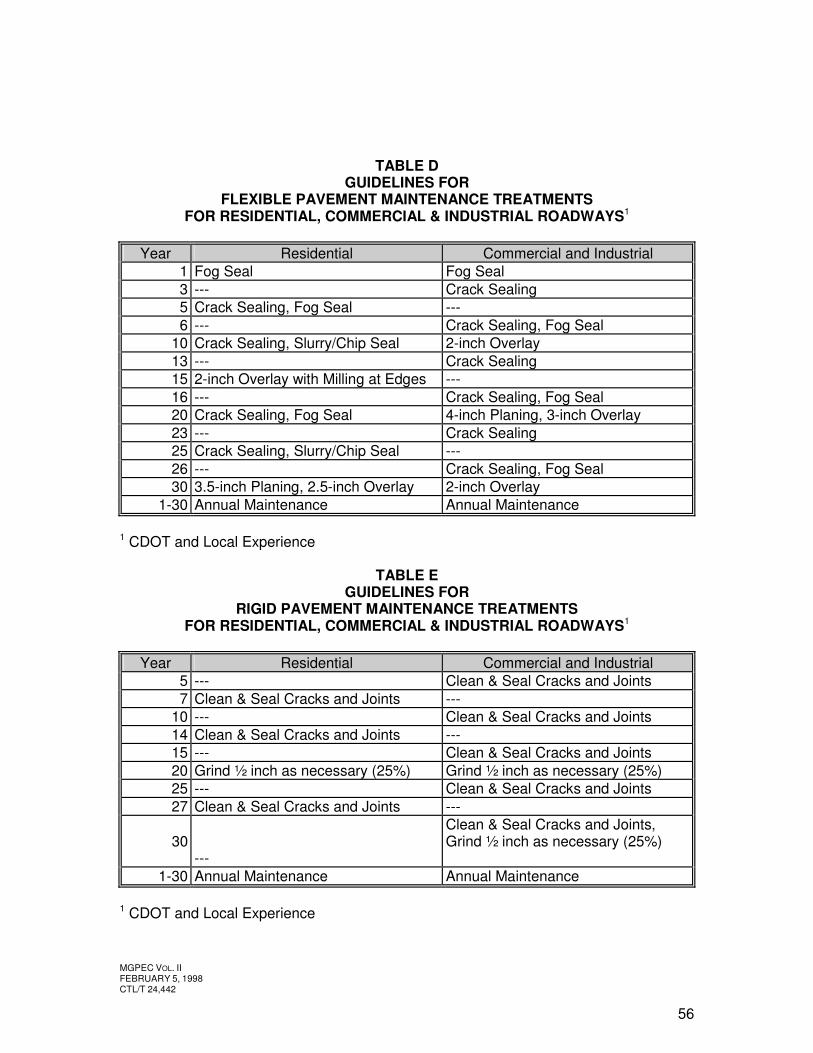
MGPEC VOL. II FEBRUARY 5, 1998 CTL/T 24,442
56
TABLE D GUIDELINES FOR
FLEXIBLE PAVEMENT MAINTENANCE TREATMENTS FOR RESIDENTIAL, COMMERCIAL & INDUSTRIAL ROADWAYS1
Year Residential Commercial and Industrial
1 Fog Seal Fog Seal 3 --- Crack Sealing 5 Crack Sealing, Fog Seal --- 6 --- Crack Sealing, Fog Seal
10 Crack Sealing, Slurry/Chip Seal 2-inch Overlay 13 --- Crack Sealing 15 2-inch Overlay with Milling at Edges --- 16 --- Crack Sealing, Fog Seal 20 Crack Sealing, Fog Seal 4-inch Planing, 3-inch Overlay 23 --- Crack Sealing 25 Crack Sealing, Slurry/Chip Seal --- 26 --- Crack Sealing, Fog Seal 30 3.5-inch Planing, 2.5-inch Overlay 2-inch Overlay
1-30 Annual Maintenance Annual Maintenance 1 CDOT and Local Experience
TABLE E GUIDELINES FOR
RIGID PAVEMENT MAINTENANCE TREATMENTS FOR RESIDENTIAL, COMMERCIAL & INDUSTRIAL ROADWAYS1
Year Residential Commercial and Industrial
5 --- Clean & Seal Cracks and Joints 7 Clean & Seal Cracks and Joints ---
10 --- Clean & Seal Cracks and Joints 14 Clean & Seal Cracks and Joints --- 15 --- Clean & Seal Cracks and Joints 20 Grind ½ inch as necessary (25%) Grind ½ inch as necessary (25%) 25 --- Clean & Seal Cracks and Joints 27 Clean & Seal Cracks and Joints ---
30
---
Clean & Seal Cracks and Joints, Grind ½ inch as necessary (25%)
1-30 Annual Maintenance Annual Maintenance 1 CDOT and Local Experience
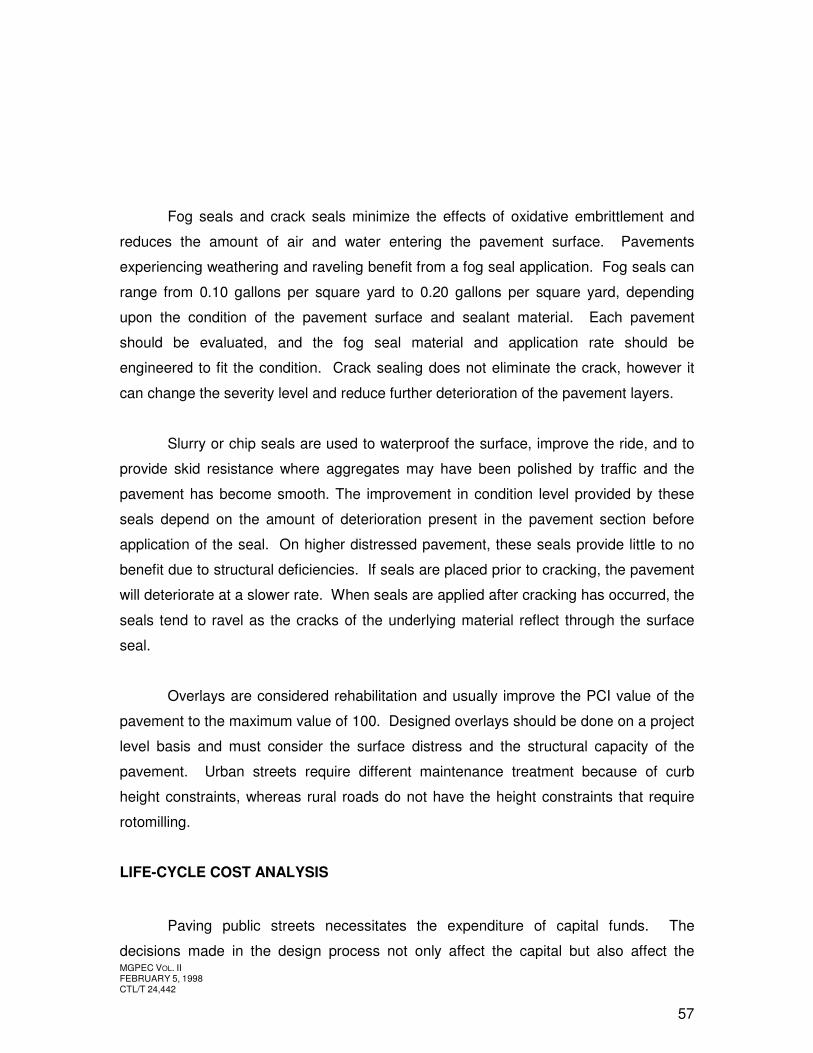
MGPEC VOL. II FEBRUARY 5, 1998 CTL/T 24,442
57
Fog seals and crack seals minimize the effects of oxidative embrittlement and
reduces the amount of air and water entering the pavement surface. Pavements
experiencing weathering and raveling benefit from a fog seal application. Fog seals can
range from 0.10 gallons per square yard to 0.20 gallons per square yard, depending
upon the condition of the pavement surface and sealant material. Each pavement
should be evaluated, and the fog seal material and application rate should be
engineered to fit the condition. Crack sealing does not eliminate the crack, however it
can change the severity level and reduce further deterioration of the pavement layers.
Slurry or chip seals are used to waterproof the surface, improve the ride, and to
provide skid resistance where aggregates may have been polished by traffic and the
pavement has become smooth. The improvement in condition level provided by these
seals depend on the amount of deterioration present in the pavement section before
application of the seal. On higher distressed pavement, these seals provide little to no
benefit due to structural deficiencies. If seals are placed prior to cracking, the pavement
will deteriorate at a slower rate. When seals are applied after cracking has occurred, the
seals tend to ravel as the cracks of the underlying material reflect through the surface
seal.
Overlays are considered rehabilitation and usually improve the PCI value of the
pavement to the maximum value of 100. Designed overlays should be done on a project
level basis and must consider the surface distress and the structural capacity of the
pavement. Urban streets require different maintenance treatment because of curb
height constraints, whereas rural roads do not have the height constraints that require
rotomilling.
LIFE-CYCLE COST ANALYSIS
Paving public streets necessitates the expenditure of capital funds. The
decisions made in the design process not only affect the capital but also affect the
MGPEC VOL. II FEBRUARY 5, 1998 CTL/T 24,442
58
maintenance budget. These decisions consequently require that an economic analysis
be performed during the design process. Life-cycle cost analysis determines the relative
financial effectiveness of a set of alternatives over a fixed time period. This analysis
provides a means to select the preferred alternative based on estimated costs of initial
construction and future maintenance costs.
For the analysis to be valid, the analysis period of each pavement section must
be equal. Costs assumed for initial construction and maintenance operations must also
be valid and based on best estimates. Construction costs are highly erratic and time
dependent. Predictions of cost thus represent an indicator, rather than a true estimate.
Interest rates used in the analysis are often debatable and politically sensitive. High-
interest rates promote decisions based on first costs and a short-term approach;
whereas low-interest rates encourage consideration of long-term costs. The
effectiveness and service life of maintenance operations and rehabilitation operations
significantly influence cost and can create bias. However, life-cycle cost analysis is a
tool to be used by design engineers along with sound engineering practice to judge the
best design alternative based on capital and maintenance costs over the analysis period,
not just the construction costs.
The three generally accepted methods for calculating life cycle costs are the
present worth method, equivalent annual worth method, and the future worth method.
All methods calculate the cost of a project over its life. The difference is whether the
cost is measured in today’s dollars (at present worth), as a uniform series of annual
dollars (at present worth), or the cost at the end of the project life (future). The present
worth method is used by most engineers and agencies and was selected for this work.
The present worth method discounts all costs to present-day based on the
assumed discount rate (interest). The present worth of a project is equivalent to the
amount of money that would have to be invested to cover the costs of construction,
maintenance, and rehabilitation over the analysis period. Variables that must be
established to calculate present worth include discount rate (interest rate), cost definition
(cost of construction and maintenance), analysis period, salvage value, and life of
MGPEC VOL. II FEBRUARY 5, 1998 CTL/T 24,442
59
maintenance and rehabilitation alternatives. Using these values and the pavement
maintenance recommendations, the present worth can be calculated as:
Equation 19:
Where: Pw = present worth (dollars) i = discount rate (annual) I = initial construction cost (dollars) A = annualized future maintenance costs (dollars) n = number of years for analysis (number) S = salvage value (dollars) The calculation of life-cycle costs can be time consuming and subject to
significant bias. As a standard for MGPEC, it is suggested the Colorado Department of
Transportation model and computer code be used. It serves as the basis for the
analyses performed in this study.
Discount Rate
The discount rate is the effective interest rate per interest period. The discount
rate is determined by subtracting the inflation rate from the market interest rate. The
discount rate of capital has been between 3.7 and 4.4 percent since 1966 (Epps and
Wootan, 1981,25 and Corps of Engineers, 198726). The January 1997 rate is
approximately 3.8 percent, based on a 30-year bond. Based on this information, a
discount rate of 4 percent per year was used for analysis purposes in this document.
Cost Definition
The cost definition is the actual dollar value assigned to each item and procedure
defined during construction and maintenance operations for the project. The costs are
listed as present worth values for construction and predicted inflated prices for
maintenance procedures. These prices are often very susceptible to bias costing.
P SUB w = I + { A[(1+i) SUP n - 1] } OVER { i(1+i) SUP n } -S OVER { (1+i) SUP n }
MGPEC VOL. II FEBRUARY 5, 1998 CTL/T 24,442
60
A yearly cost data book, available from the Colorado Department of
Transportation (CDOT), lists the quantity of material used for CDOT projects and
associated unit prices. CDOT data for the 1995 construction season were used in this
report. Time of construction and location affect the unit prices. The costs for each
project should be determined based on projects of similar size and location. Where
CDOT cost data are not available, quotes from contractors or material suppliers can be
used. It should be noted that often these costs can be biased, and competitive quotes
should be obtained.
Analysis Period
The analysis period is the selected time period, in years, over which the
alternatives are compared. A single analysis period allows all alternatives to be
compared on a common basis. The analysis period should be chosen to allow for a
minimum of one major rehabilitation for each alternative, to account for unequal
performance of the various pavement alternatives (PCCP and ACCP). A 30-year
analysis period is recommended to allow for a minimum of one major rehabilitation for
each alternative for a twenty year design life.
Salvage Value
Salvage value is the future value of the pavement materials at the end of the
analysis period. Salvage values are assumed to be equal at the end of the analysis
period for this report, therefore canceling each other. Furthermore, it was assumed that
the ACCP and PCCP will be recycled.
Life of Maintenance Treatments
In predicting the performance of pavement sections, the design engineer should
bear in mind that maintenance and rehabilitation alternatives have significant impacts on
the life cycle cost analysis. The design engineer must be aware of the appropriateness
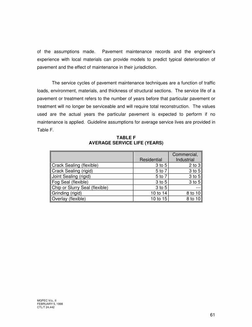
MGPEC VOL. II FEBRUARY 5, 1998 CTL/T 24,442
61
of the assumptions made. Pavement maintenance records and the engineer’s
experience with local materials can provide models to predict typical deterioration of
pavement and the effect of maintenance in their jurisdiction.
The service cycles of pavement maintenance techniques are a function of traffic
loads, environment, materials, and thickness of structural sections. The service life of a
pavement or treatment refers to the number of years before that particular pavement or
treatment will no longer be serviceable and will require total reconstruction. The values
used are the actual years the particular pavement is expected to perform if no
maintenance is applied. Guideline assumptions for average service lives are provided in
Table F.
TABLE F AVERAGE SERVICE LIFE (YEARS)
Residential Commercial,
Industrial Crack Sealing (flexible) 3 to 5 2 to 3 Crack Sealing (rigid) 5 to 7 3 to 5 Joint Sealing (rigid) 5 to 7 3 to 5 Fog Seal (flexible) 3 to 5 3 to 5 Chip or Slurry Seal (flexible) 3 to 5 --- Grinding (rigid) 10 to 14 8 to 10 Overlay (flexible) 10 to 15 8 to 10
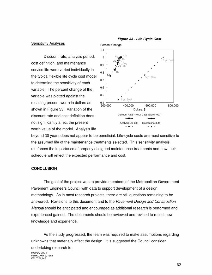
MGPEC VOL. II FEBRUARY 5, 1998 CTL/T 24,442
62
Sensitivity Analyses
Discount rate, analysis period,
cost definition, and maintenance
service life were varied individually in
the typical flexible life cycle cost model
to determine the sensitivity of each
variable. The percent change of the
variable was plotted against the
resulting present worth in dollars as
shown in Figure 33. Variation of the
discount rate and cost definition does
not significantly affect the present
worth value of the model. Analysis life
beyond 30 years does not appear to be beneficial. Life-cycle costs are most sensitive to
the assumed life of the maintenance treatments selected. This sensitivity analysis
reinforces the importance of properly designed maintenance treatments and how their
schedule will reflect the expected performance and cost.
CONCLUSION
The goal of the project was to provide members of the Metropolitan Government
Pavement Engineers Council with data to support development of a design
methodology. As in most research projects, there are still questions remaining to be
answered. Revisions to this document and to the Pavement Design and Construction
Manual should be anticipated and encouraged as additional research is performed and
experienced gained. The documents should be reviewed and revised to reflect new
knowledge and experience.
As the study progressed, the team was required to make assumptions regarding
unknowns that materially affect the design. It is suggested the Council consider
undertaking research to:
Figure 33 - Life Cycle Cost
Sensitivity Analysis
200,000 400,000 600,000 800,0000.4
0.5
0.6
0.7
0.8
0.9
1
1.1
Dollars, $
Percent Change
Discount Rate (4.0%) Cost Value (1997)
Analysis Life (30) Maintenance Life
20
30
40
4%
3%
5%
0%4%
8%
6 yr. Seal
3 yr. Seal
5 yr. Seal
MGPEC VOL. II FEBRUARY 5, 1998 CTL/T 24,442
63
1. Determine actual weights and local distribution of trash trucks. 2. Reexamine asphalt cement concrete pavement mix design philosophies
in light of high-contact stresses and comparatively poor performance of some mixes tested in this study.
3. Expand the database of material properties to better evaluate and
characterize subgrade and paving materials. 4. Accumulate and standardize cost and performance data for initial
construction and maintenance techniques.
MGPEC VOL. II FEBRUARY 5, 1998 CTL/T 24,442
64
REFERENCES 1. American Association of State Highway and Transportation Officials, AASHTO Guide
for Design of Pavement Structures, 1986. 2. AASHO Operating Subcommittee on Roadway Design, AASHO Interim Guide for
Design of Pavement Structures 1972, AASHO, Washington, D.C. 3. American Association of State Highway and Transportation Officials, AASHTO Guide
for Design of Pavement Structures, 1993. 4. V. J. Peters and G. Scot Gordon, Determination of Bus Equivalent Factors,
CTL/Thompson, Inc., Report for City and County of Denver, Colorado, 1993. 5. Asphalt Institute, A Computer Program for the Analysis (Including Seasonal
Variations) of Highway Pavements with Dual Wheel Loadings - DAMA, 1993 Edition.
6. Dar-Hao Chen, Masharraf Zaman, Joakin Laguros, and Alan Soltani, “Assessment of
Computer Programs for Analysis of Flexible Pavement Structure,” Transportation Research Record No. 1482, 1995.
7. H. L. Von Quintus, J. A. Scherocman, C. S. Hughes, and T. W. Kennedy, “Asphalt-
Aggregate Mixture Analysis System,” National Cooperative Highway Research Program Report 338, TRB, March 1991.
8. Reynaldo Rogue, Conversation with Professor at the University of Florida during
Presentation at Annual Association of Asphalt Pavement Technologists (AAPT) Conference, 1997.
9. John T. Tielking, “Aircraft Tire/Pavement Pressure Distributions,” Prepared for Air
force Engineering and Service Center, Texas Transportation Institute, MM 7111-89-1, January 1989.
10. Geo-Slope International, Calgary, Alberta, Canada, SIGMA/W, for Finite Element
Stress/Deformation Analysis, Version 3.06, September 1995. 11. G. King, H. King, O. Harders, P. Chaverot, and J. P. Planche, Influence of Asphalt
Grade and Polymer Concentration on the High Temperature Performance of Polymer Modified Asphalt Proceedings, AAPT, Vol. 61, 1992.
12. E. L. Skok, Jr., and F. N. Finn. Theoretical Concepts Applied to Asphalt Pavement
Design. Proc., International Conference on the Structural Design of Asphalt Pavements, Ann Arbor, Michigan, 1962, p. 421.
MGPEC VOL. II FEBRUARY 5, 1998 CTL/T 24,442
13. M. R. Thompson and Q. L. Robnett. Resilient Properties of Subgrade Soils, Final Report--Data Summary. Transportation Engineering Series No. 14. Illinois Cooperative Highway Research and Transportation Program Series No. 160. University of Illinois at Urbana-Champaign, 1976.
14. Dingqing Li and Ernest T. Selig. Resilient Modulus for Fine-Grained Subgrade Soils. Journal of Geotechnical Engineering, Vol. 120, No. 6, June 1994.
15. W. Lee, N. C. Bohra, A. G. Altschaeffl, and T. D. White, Resilient Modulus of Cohesive Soils, Journal of Geotechnical and Geoenvironmental Engineering, February 1997, pp. 131-136.
16. D. V. Holmquist, “Subgrade Investigation and Design of Airside Pavements at Denver International Airport,” Presentation to National Airport Conference on Pavement, 1993, Denver, Colorado.
17. Dallas N. Little, “Evaluation of the Structural Properties of Stabilized Pavement Layers,” Interim Report to the Texas Department of Transportation, Research Project 1287, 1993.
18. J. L. Cowley, P.E., “Geotextile Technology: Substitution Factors Between Mirafi Woven Stabilization Fabrics and Aggregate Base Thickness in Asphalt Pavements, Law Engineering, December 1981.
19. Dallas N. Little, “Stabilization of Pavement Subgrades and Base Courses With Lime,” National Lime Association, Kendall/Hunt Publishing Company, 1995.
20. Eric C. Drumm, Jason S. Reeves, Mark R. Madgett, and William D. Trolinger, “Subgrade Resilient Modulus Correction For Saturation Effects,” Journal of Geotechnical and Geoenvironmental Engineering, American Society of Civil Engineers, July 1997, Vol. 123, No.7.
21. E. J. Yoder and M. W. Witczak, Principles of Pavement Design, Second Edition, John Wiley & Sons, Inc., 1975.
22. G. Scot Gordon and Victoria Peters, Evaluation of Lime Stabilized Subgrade Structural Layer Coefficient, CTL/Thompson, Inc., Report for Jefferson County, Colorado, 1995.
23. M. Y. Shahin and J. A. Walter, Pavement Maintenance Management for Roads and Streets Using the PAVER System, USACERL Technical Report M-90/05, July 1990.
24. R. E. Smith, M. I. Darter, S. H. Carpenter, M. Y. Shahin, Adjusting Performance Curves for the Influence of Maintenance and Rehabilitation, ERES Consultants, Inc. for Metropolitan Transportation Commission, Oakland, California.

MGPEC VOL. II FEBRUARY 5, 1998 CTL/T 24,442
25. J. A. Epps and C. V. Wootan, Economic Analysis of Airport Rehabilitation Alternatives – An Engineering Manual, Report DOT/FAA/FD-81/78, Federal Aviation Administration, 1981.
26. U. S. Army Corps of Engineers, Life Cycle Costs for Pavements, Report F84-63, 1987.

MGPEC VOL. II FEBRUARY 5, 1998 CTL/T 24,442
APPENDIX A
SURVEY RESULTS

MGPEC VOL. II FEBRUARY 5, 1998 CTL/T 24,442
APPENDIX B
GLOSSARY OF TERMS

MGPEC VOL. II FEBRUARY 5, 1998 CTL/T 24,442
B-1
GLOSSARY OF TERMS
Adhesive Failure: Loss of bond between the joint sealant and the joint, or between the aggregate and the binder.
Aggregate Base (base course): Crushed stone or gravel, immediately under the surfacing material.
Aggregate Interlock: Interaction of aggregate particles across cracks and joints to transfer load.
Alligator Cracks: Interconnected cracks forming a series of small blocks resembling an alligator’s skin or chicken wire.
Analysis Period: The period of time for which the economic analysis is to be made; ordinarily will include at least one rehabilitation activity.
Asphalt Cement Concrete Pavement (ACCP): High-quality, thoroughly-controlled hot mixture of asphalt cement and well-graded, high quality aggregate, thoroughly compacted into a uniform dense mass.
Asphalt Emulsion Slurry Seal: A mixture of emulsified asphalt, fine aggregate and mineral filler, with water added to produce slurry consistency.
Asphalt Leveling Course: A course (asphalt-aggregate mixture) of variable thickness used to eliminate irregularities in the contour of an existing surface prior to superimposed treatment or construction.
Asphalt Overlay: One or more courses of asphalt construction on an existing pavement. The overlay generally includes a leveling course, to correct the contour of the old pavement, followed by uniform course or courses to provide needed thickness.
Asphalt Cement Concrete Pavements: Pavements consisting of a surface course of mineral aggregate coated and cemented together with asphalt cement on supporting courses such as asphalt bases; crushed stone, slag or gravel; or on Portland cement concrete pavement, brick, or block pavement.
Asphalt Cement Concrete Pavement Structure: A pavement structure, placed above the natural subgrade, with courses consisting of asphalt-aggregate mixtures, untreated aggregate courses, improved or stabilized subgrade, drainage layers, etc. which act in a structural capacity.
MGPEC VOL. II FEBRUARY 5, 1998 CTL/T 24,442
B-2
Asphalt Tack Coat: A light application of emulsified asphalt applied to an existing asphalt or Portland cement concrete pavement surface. It is used to ensure a bond between the surface being paved and the overlying course. Typically 0.10 gals/yd2 of CSS1h.
Binder: Asphalt Cement used to hold stones together for paving.
Binder Course: The layer of asphalt cement concrete pavement underlying the surface course.
Bituminous: Like or from asphalt.
Bleeding or Flushing: The upward movement of asphalt in an asphalt pavement resulting in the formation of a film on the pavement surface. It creates a shiny, glass-like, reflective surface that may be tacky to the touch in warm weather.
Block Cracking: The occurrence of cracks that divide the asphalt surface into approximately rectangular pieces, typically one square foot or more in size.
California Bearing Ratio Test (CBR): An empirical measure of bearing capacity used for evaluating bases, subbases, and subgrades for pavement thickness design.
Centerline: The painted line separating opposing traffic lanes.
Channels: See Rutting.
Chipping: Breaking or cutting off small pieces from the surface.
Chip Seal: A thin layer of emulsified asphalt cement in which aggregate is embedded. The seal is placed to improve the texture of the pavement surface to increase skid resistance and decrease permeability of the surface.
City Street: A street whose traffic is predominantly local in character.
Cohesive Failure: The loss of a material’s ability to bond to itself or its substrate. Results in the material splitting or tearing apart from itself or its substrate (i.e. joint sealant splitting).
Composite Pavement: A pavement structure composed of an asphalt cement concrete pavement wearing surface and Portland cement concrete pavement slab; an asphalt cement concrete pavement overlay on a PCC slab is also referred to as a composite pavement.
Corrugations (Washboarding): A form of plastic movement typified by ripples across the pavement surface. Most common in aggregate surficial pavements but occurs in asphalt cement concrete pavements as well.
Crack: Approximately vertical random cleavage of the pavement due to thermal or load action.
MGPEC VOL. II FEBRUARY 5, 1998 CTL/T 24,442
B-3
Deflection: The amount of downward vertical movement of a surface due to the application of a load to the surface.
--Rebound Deflection: The amount of vertical rebound of a surface that occurs when a load is removed from the surface.
--Representative Rebound Deflection: The mean value of measured rebound deflections in a test section plus two standard deviations, adjusted for temperature and most critical period of the year for pavement performance.
--Residual Deflection: The difference between original and final elevations of a surface resulting from the application to, and removal of one or more loads from, the surface.
Design ESAL: The total number of equivalent 80kN (18,000 lb) single-axle load applications expected during the Design Period.
Design Lane: The lane on which the greatest number of equivalent 80kN (18,000 lb) single-axle loads is expected. Normally this will be either lane of a two-lane roadway or the outside lane of a multi-lane highway.
Design Period: The number of years from initial construction or rehabilitation until terminal service life. This term should not be confused with pavement life or Analysis Period. By adding asphalt overlays as required, pavement life may be extended indefinitely, or until geometric considerations or other factors make the pavement obsolete.
Disintegration: The breaking up of a pavement into small, loose fragments due to traffic or weathering.
Distortion: Any change of a pavement surface from its original shape.
Drainage Coefficients: Factors used to modify layer coefficients in flexible pavements or stresses in rigid pavements as a function of how well the pavement structure can handle the adverse effect of water infiltration.
Edge Cracking: Fracture and materials loss in pavements without paved shoulders which occurs along the pavement perimeter. Caused by soil movement beneath the pavement.
Effective Thickness: The thickness that a pavement would be if it could be converted to Full-Depth asphalt cement concrete pavement.
Embankment (embankment soil): The prepared or natural soil underlying the pavement structure.
Embrittlement: Premature (surficial) cracking of an asphalt concrete pavement due to oxidative aging of the asphalt cement.
MGPEC VOL. II FEBRUARY 5, 1998 CTL/T 24,442
B-4
End Result Specifications: Specifications that require the contractor to take the entire responsibility for supplying a product or an item of construction. The highway agency’s responsibility is to either accept or reject the final product or apply a price adjustment that compensates for the degree of compliance with the specifications. (End result specifications have the advantage of affording the contractor flexibility in exercising options for using new materials, techniques, and procedures to improve the quality and/or economy of the end product.)
ESAL to Failure: The number of design 18 kip axle load cycles required to produce approximately 40 percent fatigue cracking as calculated using AAMAS equations based on asphalt cement concrete pavement Resilient Modulus and tensile strain at the bottom of the ACCP layer.
Equivalent 80kN (18,000 lb) Single-Axle Load (ESAL): The effect on pavement performance of any combination of axle loads of varying magnitude equated to the number of 80kN (18,000 lb) single-axle loads required to produce an equivalent effect.
Fatigue Cracking: A series of small, jagged, interconnecting cracks caused by failure of the asphalt cement concrete pavement surface under repeated traffic loading (also called alligator cracking.)
Fault: Difference in elevation between opposing sides of a joint or crack.
Flexible Pavement: see Pavement.
Free Edge: Pavement border that is able to move freely.
Full-Depth Asphalt Pavement: The term FULL-DEPTH (registered by the Asphalt Institute with the U.S. Patent Office) certifies that the pavement is one in which asphalt mixtures are employed for all courses above the subgrade or improved subgrade. A Full-Depth asphalt pavement is laid directly on the prepared subgrade.
Functional Classification: A method of separating and classifying streets according to their purpose or function in the network of streets, i.e. residential collectors, commercial collectors, residential locals.
Grade Depressions: Localized low areas of limited size which may or may not be accompanied by cracking.
Hairline Crack: A fracture that is very narrow in width, less than 3mm (0.12 in.).
Heavy Trucks: Two axle, six-tire trucks or larger. Pickup, panel and light four-tire trucks are not included. Trucks with heavy-duty, wide base tires are included.
Hydroplaning: The dangerous action of a vehicle being driven on a pavement over which a film of rain or other water has formed; on reaching a certain speed, the vehicle’s tires tend to ride upon the water surface rather than the pavement, drastically reducing the driver’s control of the vehicle.
MGPEC VOL. II FEBRUARY 5, 1998 CTL/T 24,442
B-5
Incentive/Disincentive Provision (for quality): A pay adjustment schedule which functions to motivate the contractor to provide a high level of quality. (A pay adjustment schedule, even one which provides for pay increases, is not necessarily an incentive/disincentive provision, as individual pay increases/decreases may not be of sufficient magnitude to motivate the contractor toward high quality.)
Instability: The lack of resistance to forces tending to cause movement or distortion of a pavement structure.
Lane Line: Boundary between travel lanes, usually a painted stripe.
Lane-to-Shoulder Drop-off: The difference in elevation between the traffic lane and shoulder.
Lane-to-Shoulder Separation: Widening of the joint between the traffic lane and the shoulder.
Layer Coefficient: The empirical relationship between structural number (SN) and layer thickness which expresses the relative ability of a material to function as a structural component of the pavement.
Lime Stabilized Subgrade: A prepared and mechanically compacted mixture or lime, water and soil below the pavement system.
Lime-Fly Ash Base: A blend of mineral aggregate, lime, fly ash and water, combined in proper proportions which, when compacted, produces a dense mass.
Load Equivalency Factor (LF): A factor used to convert applications of axle loads of any magnitude to an equivalent number of 80kN (18,000 lb) single axle loads.
Longitudinal: Parallel to the centerline of the pavement.
Longitudinal Crack: A crack that follows a course approximately parallel to the center line.
Maintenance: The preservation of the entire roadway, including surface, shoulders, roadsides, structures, and such traffic control devices as are necessary for its safe and efficient utilization.
Materials/Methods Specifications: Specifications that direct the contractor to use specified materials in definite proportions and specific types of equipment and methods to place the material.
Method Specifications: see Materials/Methods Specifications.
Parametric Analysis: A study of a set of physical properties whose values determine the characteristics or behavior of something. Used to isolate the significance of individual variables.
MGPEC VOL. II FEBRUARY 5, 1998 CTL/T 24,442
B-6
Patch: An area where the existing pavement has been removed and replaced with a new material.
Patch Deterioration: Distress occurring within a previously repaired area.
Pavement Structure (pavement): A combination of subbase, base course, and surface course placed on a subgrade to support the traffic load and distribute it to the roadbed.
Pavement Condition Indicator (PCI): A measure of the condition of an existing pavement section at a particular point in time, such as cracking measured in feet per mile, or faulting measured in inches of wheelpath faulting per mile. When considered collectively, pavement condition indicators provide an estimate of the overall adequacy of a particular roadway.
Pavement Design (design, structure design): The specifications for materials and thicknesses of the pavement components .
Pavement Distress Indicator: see Pavement Condition Indicator.
Pavement, Flexible: A pavement structure generally consisting of asphalt cement concrete pavement surfacing, base and/or subbase.
Pavement Performance: The trend of serviceability with load applications.
Pavement Rehabilitation: Work undertaken to extend the service life of an existing facility. This includes placement of additional surfacing material and/or other work necessary to return an existing roadway, including shoulders, to a condition of structural or functional adequacy. This could include the complete removal and replacement of the pavement structure.
Pavement, Rigid: A pavement structure consisting of Portland cement concrete pavement surfacing, with or without subbase.
Performance Period: see Design Period.
Performance Specifications: Specifications that describe how the finished product should perform over time. For highways, performance is typically described in terms of changes in physical condition of the surface and its response to load, or in terms of the cumulative traffic required to bring the pavement to a condition defined as “failure”. Specifications containing warranty/guarantee clauses are a form of performance specifications. (Other than the warranty/guarantee type, performance specifications have not been used for major highway pavement components (subgrades, bases, riding surfaces) because there have not been appropriate nondestructive tests to measure long-term performance immediately after construction. They have been used for some products (e.g., highway lighting, electrical components, and joint sealant materials) for which there are test of performance that can be rapidly conducted.)
Performance-Based Specifications: Specifications that describe the desired levels of fundamental engineering properties (e.g., Resilient Modulus, creep properties, and
MGPEC VOL. II FEBRUARY 5, 1998 CTL/T 24,442
B-7
fatigue properties) that are predictors of performance and appear in primary prediction relationships (i.e., models that can be used to predict pavement stress, distress, or performance from combinations of predictors that represent traffic, environmental roadbed, and structural conditions.) [Because most fundamental engineering properties associated with pavements are currently not amenable to timely acceptance testing, performance-based specifications have not found application in highway construction].
Performance-Related Specifications: Specifications that describe the desired levels of key materials and construction quality characteristics that have been found to correlate with fundamental engineering properties that predict performance. These characteristics (for example, air voids in asphaltic pavements, and strength of concrete cores) are amenable to acceptance testing at the time of construction. True performance-related specifications not only describe the desired levels of these quality characteristics, but also employ the quantified relationships containing the characteristics to predict subsequent pavement performance. They thus provide the basis for rational acceptance and/or price adjustment decisions.
Planned Stage Construction: The construction of roads and streets by applying successive layers of asphalt cement concrete pavement according to design and a predetermined time schedule.
Plant-Mix Base: A foundation course, produced in an asphalt mixing plant, which consists of a mineral aggregate uniformly coated with asphalt cement or emulsified asphalt.
Pothole: A bowl-shaped depression of varying sizes in the pavement surface, resulting from localized disintegration.
Prepared Roadbed: In-place roadbed soils compacted or stabilized according to provisions of applicable specifications.
Prescriptive Specifications: see Materials/Methods Specifications.
Present Serviceability: The ability of a specific section of pavement to serve, for the use intended, mixed traffic on the day of rating.
Present Serviceability Index (PSI): A mathematical combination of values, obtained from certain physical measurements of a large number of pavements, so formulated as to predict, within prescribed limits, the Present Serviceability Rating (PSR) for those pavements.
Present Serviceability Rating (PSR): The mean of the individual ratings made by the members of a specific panel selected for the purpose.
QA/QC Specifications: see Quality Assurance Specifications.
QC/QA Specifications: see Quality Assurance Specifications.
MGPEC VOL. II FEBRUARY 5, 1998 CTL/T 24,442
B-8
Quality Assurance: All those planned and systematic actions necessary to provide confidence that a product or facility will perform satisfactorily in service. Quality assurance addresses the overall problem of obtaining the quality of service, product, or facility in the most efficient, economical, and satisfactory manner possible. Within this broad context, quality assurance involves continued evaluation of the activities of planning, design, development of plans and specifications, advertising and awarding of contracts, construction, and maintenance, and the interactions of these activities.
Quality Assurance Specifications: A combination of end result specifications and materials and methods specifications. The contractor is responsible for quality control (process control), and the highway agency is responsible for acceptance of the product. (Quality assurance specifications typically are statistically based specifications that use methods such as random sampling and lot-by-lot testing, which let the contractor know if his operations are producing an acceptable product.)
Quality Control: Those quality assurance actions and considerations necessary to assess production and construction processes so as to control the level of quality being produced in the end product. This concept of quality control includes sampling and testing to monitor the process but usually does not include acceptance sampling and testing.
Raveling: The wearing away of the pavement surface caused by the dislodging of aggregate particles.
Recipe Specifications: see Materials/Methods Specifications.
Reflection Cracking: Cracks in asphalt overlays that reflect the crack pattern in the pavement structure underneath.
Resilient Modulus Test: A measure of the modulus of elasticity of roadbed soil or other pavement material.
Resistance Value (R-value): A test for evaluating bases, subbases, and subgrades for pavement thickness design.
Roadbed: The graded portion of a highway between top and side slopes, prepared as a foundation for the pavement structure and shoulder.
Roadbed Material: The material below the subgrade in cuts and embankments and in embankment foundations, extending to such depth as affects the support of the pavement structure.
Roadway: All facilities on which motor vehicles are intended to travel such as secondary roads, interstate highways, streets and parking lots.
Roadway Land Use: A classification based on the use of land adjacent or serviced by the street. The classification is used to separate streets for different volume assumptions.
MGPEC VOL. II FEBRUARY 5, 1998 CTL/T 24,442
B-9
Roughometer: A single-wheeled trailer instrumented to measure the roughness of a pavement surface in accumulated millimeters (inches) per mile.
Rubberized Asphalt Cement: Blend of asphalt cement and pre-vulcanized rubber.
Rutting: Longitudinal surface depressions in the wheelpaths.
Selected Material: A suitable native material obtained from a specified source such as a particular roadway cut or borrow area, of a suitable material having specified characteristics to be used for a specific purpose.
Serviceability: The ability at time of observation of a pavement to serve traffic (autos and trucks) which use the facility.
Shoving: Permanent, longitudinal displacement of a localized area of the pavement surface caused by traffic pushing against the pavement.
Single Axle Load: The total load transmitted by all wheels of a single axle extending the full width of the vehicle.
Skid Hazard: Any condition that might contribute to making a pavement slippery when wet.
Slippage Cracks: Cracks, sometimes crescent-shaped, that point in the direction of the thrust of wheels on the pavement surface.
SMA (Stone-Matrix Asphalt, Split-Mastic Asphalt): An asphalt mix design composed of large stones creating a stone to stone matrix, often containing large percentages of asphalt cement and fillers.
Soil Cement Base: A hardened material formed by curing a mechanically compacted intimate mixture of pulverized soil, Portland cement and water, used as a layer in a pavement system to reinforce and protect the subgrade or subbase.
Stabilized Subgrade: A subgrade soil that has been altered by a chemical agent to make suitable for subgrade construction and pavement support.
Standard Deviation: The root-mean-square of the deviations about the arithmetic mean of a set of values.
Statistically Based Specifications: Specifications based on random sampling, and in which properties of the desired product or construction are described by appropriate statistical parameters.
Structural Number (SN): An index number derived from an analysis of traffic, roadbed soil conditions, and environment which may be converted to thickness of flexible pavement layers through the use of suitable layer coefficients related to the type of material being used in each layer of the pavement structure.

MGPEC VOL. II FEBRUARY 5, 1998 CTL/T 24,442
B-10
Subbase: The layer or layers of specified or selected material of designed thickness placed on a subgrade to support a base course.
Subbase (subbase course): The layer of graded sand-gravel or stabilized subgrade material between the surface of the embankment soil and the base course (or surfacing course when there is no base course).
Subgrade: The soil prepared to support a structure of a pavement system. It is the foundation for the pavement structure. The subgrade soil sometimes is called “basement soil” or “foundation soil”.
Subgrade, Improved: Any course or courses of select or improved material between the subgrade soil and the pavement structure.
Subgrade Resilient Modulus: The modulus of the subgrade determined by repeated load triaxial compression tests on soil samples. It is the ratio of the amplitude of the accepted axial stress to the amplitude of the resultant recoverable axial strain.
Surface (Surface Course): One or more layers of a pavement structure designed to accommodate the traffic load, the top layer of which resists skidding, traffic abrasion, and the disintegrating effects of climate. The top layer of flexible pavements is sometimes called the “wearing course”.
Surface Thickness (surfacing thickness, surface, slab thickness (rigid)): The thickness of surfacing materia, usually expressed in inches.
Tandem Axle Load: The total load transmitted to the road by two consecutive axles extending across the full width of the vehicle.
Thermal Cracking: Cracking occurring in pavement material introduced within the material resulting from a change in temperature.
Traffic Equivalence Factor: A numerical factor that expresses the relationship of a given axle load to another axle load in terms of their effect on the serviceability of a pavement structure.
Transverse Crack: A crack that follows a course approximately at right angles to the centerline.
Triple (Tridem) Axle Load: The total load transmitted to the road by three consecutive axles extending across the full width of the vehicle.
Truck Factor: The number of equivalent 80kN (18,000 lb) single-axle load applications contributed by one usage of a vehicle. Truck Factors can apply to vehicles of a single type or class or to a group of vehicles of different types.
Twenty-Year ESAL: (ESAL20) The Equivalent Single Axle Load application for a twenty-year design. The value is the product of the Load Equivalency factor for each vehicle
MGPEC VOL. II FEBRUARY 5, 1998 CTL/T 24,442
B-11
type, the number of each particular vehicles per day, 365 days per year, and a twenty-year period.
Upheaval: The localized upward displacement of a pavement due to swelling of the subgrade or some portion of the pavement structure.
Washboarding: see Corrugations.
Water Bleeding: Seepage of water from joints or cracks.
Weathering: The wearing away of the pavement surface caused by the loss of asphalt binder.

MGPEC VOL. II FEBRUARY 5, 1998 CTL/T 24,442
B-12
APPENDIX C
ANNOTATED LITERATURE REVIEW

MGPEC VOL. II FEBRUARY 5, 1998 CTL/T 24,442
APPENDIX D
WARRANTIES AND QUALITY ASSURANCE / QUALITY CONTROL

MGPEC VOL. II FEBRUARY 5, 1998 CTL/T 24,442
B-1
QUALITY CONTROL / QUALITY ASSURANCE / WARRANTIES
Any discussion of quality must consider the Engineer’s, Contractor’s and Owner’s
perspectives. Owners must first decide the level of control they wish to exert over the
Contractor’s operations. There are three levels of control; 1) complete testing and
inspection, 2) oversight testing, or 3) warranty control. Each of these levels requires a
different type of specification from the Engineer and a different level of effort by the
Contractor.
The most difficult specification to develop is the procedural specification. This
specification dictates to the Contractor what to build, what to build it from and how to
build it. It is the easiest type of specification for the Owner to test and inspect. It is
prescriptive in nature and easily lends itself to a “cookbook” procedure. The Owner can
impose penalties or price reduction if the Contractor does not follow the recipe.
Unfortunately, most penalties are only token in nature and seldom reflect the actual cost
to the public. For instance, analyses have shown that asphalt cement concrete
pavement compacted to 90 percent rather than 93 percent will lose 20 to 50 percent of
its service life, while penalties are less than 10 percent. Warranties for this type of
specification are typically one to 3 years in length and only cover workmanship and
materials. The procedural specification can be tempered to some extent by providing
performance criteria rather than procedural. For instance, the specification may require
compaction to 95 percent rather than “a minimum of six passes with a 20-ton steel wheel
roller at 3 mph.”
This modified procedure/performance specification is the most common in the
industry. It serves to specify certain procedures at times and performance criteria for
other items. It is easily tested and inspected and provides the Owner with control over
the project and some recourse to penalties, price reduction and warranties.
The Quality Control / Quality Assurance or oversight testing specification is normally
applicable only to large projects. In this type of specification, the Contractor is
responsible for his own quality both in terms of materials and procedures. The
Contractor is required to develop a QC plan and provide testing and inspection of his
own work. The Owner’s testing and inspection is largely oversight in nature and usually

MGPEC VOL. II FEBRUARY 5, 1998 CTL/T 24,442
B-2
involves 10 to 15 percent of the Contractor’s QC effort. Like the procedural
specification, the QA/QC specification can have both procedural and performance
components as well as penalties and price reductions. Warranties are likewise limited to
workmanship and materials. CDOT has been using the QA/QC specification on a limited
basis. Both Denver International Airport and E-470 use or used QA/QC specifications.
Experience to date has been mixed. Some contracts have worked well while other have
been nightmares leading to litigation.
The last type of specification is warranties. This is a relatively new form of contract
specification in the U. S.; but has been successfully used in Europe for years. Warranty
periods are typically 5 years in the U. S. and more often 10 years in Europe. This
specification will have limited testing and inspection on the Owner’s part and must not be
restrictive. An Owner cannot require specific procedures, nor materials in the design.
For instance, the Owners cannot specify an asphalt mix then expect the Contractor to
warrant the mix against rutting or raveling. Furthermore, the Owner cannot ask the
Contractor to warrant things beyond his control. The development of a warranty
specification must be a joint effort between the Owner, Engineer and Contractor. The
warranty specification must address measurement of performance. Asphalt pavements
will not be in perfect condition after 5 years of service. The questions then become; How
much distress and of what type is allowed? Other issued in warranties include:
1) Who is responsible for maintenance and at which intervals?
2) What if the traffic load changes?
3) Are there penalties and price reductions imposed during construction? If so, what basis?
4) What are the bonding requirements?
5) Should Contractors be pre-qualified?
6) How does the Contractor share design responsibility?
It is believed that warranty specifications will become more popular in the future.
The projects built to date appear to be successful and success will promulgate similar
MGPEC VOL. II FEBRUARY 5, 1998 CTL/T 24,442
B-3
programs. Major projects lend themselves to warranties, particularly design/build. At
this time, warranty projects offer little to the municipality or county. The time and effort
involved with specification development would tax the abilities of most agencies.
The QA/QC specification is attractive because the costs associated with testing and
inspection can be rolled into construction budgets. The experience base with the
contracting community is very limited and the previous projects have not been totally
successful. For these reasons, it is recommended to not implement QA/QA
specifications. Given time and direction by CDOT, Contractors will become more
comfortable and proficient. Likewise, warranty specifications are too new to develop any
experience base and should be reviewed at a later date. Exceptions to these
recommendations include a large project, particularly design/build where sufficient time
and cooperation between the parties are likely.
At this time, the more common procedural/performance specification is most
appropriate for municipalities and counties. The agencies should keep control through
testing and inspection. Penalties and price reduction should be carefully evaluated and
should reflect life and serviceability reduction. Specifications should also consider
remedial measures to correct or replace defective work and/or materials.

MGPEC VOL. II FEBRUARY 5, 1998 CTL/T 24,442
B-4
APPENDIX E
MATERIAL TEST RESULTS


