Development of Scenario-Based Fault Injection Platform and Its Application Study

Development of Scenario-Based Fault Injection

Platform and Its Application Study

Yung-Yuan Chen1* and Gene Eu Jan2

1Department of Computer Science and Information Engineering, Chung-Hua University,

Hsinchu, Taiwan 300, R.O.C.2Graduate Institute of Electrical Engineering, National Taipei University,

Taipei, Taiwan, R.O.C.

Abstract

This paper presents a comprehensive fault-tolerant verification platform which can be used to

characterize the impact of fault attribute on error coverage. The core of the verification platform is the

scenario-based fault injection tool that can inject the transient and permanent faults into VHDL models

of digital systems at chip, RTL and gate levels during the design phase. Weibull fault distribution is

employed to decide the time instant of fault injection. A new feature of our tool is to offer users the

statistical analysis of the injected faults. The statistical data for each injection campaign exhibit the

degree of fault severity, which represents a fault scenario (or called fault environment). By varying the

fault attributes, such as the fault duration or fault-occurring rate, we can produce a variety of fault

scenarios for the fault simulations. Such simulations can reveal the error coverage of the fault-robust

systems under various fault environments. Two case studies with experiments of fault injection were

conducted to show how the fault attribute affects the error coverage.

Key Words: Dependability Analysis, Error Coverage, Fault Attribute, Fault Injection, Fault Scenario,

Fault-Tolerant Verification Platform

1. Introduction

The dependability of fault-tolerant systems should

be validated by fault injection techniques. Three kinds of

fault injection schemes [1�4]: physical fault injection,

software-implemented fault injection and simulation-

based fault injection are implemented to inject the faults

into the hardware systems. The physical fault injection

injects the faults at the IC pin-level or by heavy-ion ra-

diation or by interference with the IC power supplies.

Software-implemented fault injection [5] is performed

by mutating code and corrupting program state vari-

ables. A major limitation of these approaches is that de-

pendability evaluation is performed after physical sys-

tems have been built. While dependability evaluation is

necessary after systems have been built, the costs of re-

designing systems due to inadequate dependability can

be prohibitively expensive.

The simulation-based fault injection [6�10] uses the

simulation to inject faults in simulation models of sys-

tems. The simulation model of system can be described

in hardware description language like VHDL. The ad-

vantage of simulation-based fault injection mechanism

is that the system dependability can be assessed as early

in the design phase, and if necessary to re-design the sys-

tem, the cost of re-design is reduced significantly. There

are two categories of techniques [6] to inject the faults

into VHDL models. First one employs the built-in com-

mands of simulator to inject the faults in simulation

models. Second category adopts the mutation of VHDL

codes to control the fault injection. The feature of first

category is easy to implement the fault injection, but the

capability is constrained by the command languages of

the simulators. The feature of second category of tech-

Tamkang Journal of Science and Engineering, Vol. 13, No. 2, pp. 205�214 (2010) 205

*Corresponding author. E-mail: [email protected]

niques is contrary to the first one.

In this work, we develop a fault injection tool based

on simulation-based injection approach. A new charac-

teristic of our tool is to offer users the statistical analysis

of the injected faults. The fault analysis is useful in that it

can facilitate us in deciding whether the fault set gener-

ated from the injection tool satisfies our need or not. If a

fault set created is similar to the previous one, then we

discard it. Thus, we can avoid performing the similar

fault sets which have been carried out before. So, a lot of

simulation time can be saved. The statistical data for

each fault set represents a fault scenario or fault envi-

ronment that indicates the degree of fault activity or

fault severity. In other words, the probability of i faults

(denoted as Pi) occurring concurrently while the fault-

tolerant system is simulated in the injection campaign

represents a fault scenario, where i � 1. For example, P1

= 97% and P2 = 3% (fault scenario 1) means that

throughout the injection campaign, when the faults oc-

cur, 97% is one fault and 3% is two faults. Compared to

P1 = 80%, P2 = 12% and P3 = 8% (fault scenario 2), it is

evident that fault scenario 2 is more severe than fault

scenario 1. By varying the fault attributes, our injection

tool can generate diverse fault environments, which can

be used to effectively validate the capability and the st-

rength of a fault-tolerant system under various fault sce-

narios. As a result, the validation process will be more

comprehensive and complete. In a word, the proposed

verification platform by integrating the enhanced fault

injection tool with ModelSim VHDL simulator and data

analyzer helps us raise the simulation efficiency and va-

lidity of the dependability analysis. The verification plat-

form is then exploited to validate the dependability of

our fault-tolerant processors and to show the impact of

fault attributes on error coverage.

The remainder of this paper is organized as follows.

Next section describes the overview of the injection tool.

The statistical analysis of fault injection campaign is pre-

sented in Section 3. The following section depicts a com-

plete verification platform. Section 5 uses the case stu-

dies to demonstrate how the fault attributes affect the

error coverage. The conclusions are drawn in Section 6.

2. Overview of the Fault Injection Tool

A tool performing fault injection into VHDL models

at chip-level, register-level and gate-level has been de-

veloped. The tool adopts the built-in commands of Mo-

delSim simulator to inject the faults into VHDL simula-

tion models. The tool consists of two phases: Phase one

is to parse the VHDL code and the desirable fault target

list is generated in this phase; the fault targets correspond

to the declaration lists of variables and signals in the

VHDL description. Phase two is to generate the fault in-

jection command file which will be used in the simula-

tion campaign.

2.1 Tool Implementation

The following information is offered to produce a

fault: when to inject a fault; where to place the fault;

what the type and value of the fault and fault duration.

Fault model used in fault injection tool comprises stuck-

at faults, indetermination and open-line (high-imped-

ance) faults. Fault duration is used to produce the tran-

sient and permanent faults and to control the length of

transient faults. Time instant of the fault injection is ac-

cording to the Weibull probability distribution, typical of

the transient faults [11], in the range: [0, tworkload], where

tworkload is the fault-free simulation duration of workload.

Next, we briefly depict how to determine the time instant

of faults.

2.2 Fault Time Instant Generation

The failure rate function associated with the Weibull

distribution is given in expression (1) and Figure 1. Para-

meter � decides the phase of z(t). If the value of � is 1,

z(t) is in useful-life period, where failure rate � is con-

stant. If � is greater than 1, z(t) is in wear-out phase; else,

z(t) is in burn-in phase. Time instant of a fault is deter-

mined by the inverse function of CDF(z(t)).

z(t) = ��(�t)��1 (1)

Note that only one phase (burn-in, useful-life or

wear-out) is determined by a specific �. However, as

shown in Figure 1(b), we may want to perform some ex-

periments where the time instant of faults injected in the

simulation campaign complies with more than one phase

of fault distributions. Figure 1(b) demonstrates an injec-

tion campaign comprises three phases of fault distribu-

tions. How to achieve the phase combination as shown in

Figure 1(b) is described below.

As can be seen from Figure 2(a), for � < 1, we can

206 Yung-Yuan Chen and Gene Eu Jan

find out t1 such that z(t1) = �; similarly, for � > 1, we can

find out t2 such that z(t2) = �. So, z(t) in Figure 2(a) has

two threshold points, one t1 and another t2. Therefore, by

means of t1 and t2, in Figure 2(b), we can compute their

respective CDF values, x and y. Then, the phase com-

bination can be accomplished in the following way:

CDF(z(t)) < x is in burn-in region; x � CDF(z(t)) � y is in

useful-life region and CDF(z(t)) > y is in wear-out re-

gion. Our tool offers the capability to let users choose the

phase combination in each injection campaign. Three

categories of phase combinations, namely single, partial

and full, are provided. Single phase uses one phase of

distribution to generate the time instant of fault injection;

partial category provides two options: one is burn-in plus

useful-life phases and the other is useful-life coupled

with wear-out phases; finally, full phase combination

consists of three phases as shown in Figure 2(b).

3. Statistical Analysis of Fault Injection

Fault injection tool can produce the injection com-

mand files, which will be used in the simulation to vali-

date the fault-tolerant systems. Each injection command

file created is based on a set of parameters including, for

example, fault types, fault duration, fault-occurring rate

(or called fault frequency) and fault distribution. Each

injection command file represents a specific fault sce-

nario or fault environment. Thus, we can adjust the tool

parameters to generate the desirable fault scenarios that

can be exploited to verify the robustness of fault-tolerant

systems under different degrees of severity of faults.

In this tool, we provide a new idea which can offer

the statistical analysis of each injection campaign such

that the fault scenario associated with an injection cam-

paign can be revealed from the statistical data. The statis-

tical analysis of injection campaigns is able to disclose

the fault activity within the simulation. Several notations

are developed first:

� NF: total number of faults injected in an injection

campaign;

� LT: total length of time that the faults occur during the

simulation;

� Ti: length of time that i faults happen concurrently dur-

ing the simulation, 1 � i � max, where max is the maxi-

mum number of faults existing in the simulated system

simultaneously;

Development of Scenario-Based Fault Injection Platform and Its Application Study 207

Figure 1. (a) failure rate function. (b) CDF of failure rate function.

Figure 2. Thresholds of phases.

� Pi: probability of i faults occurring concurrently while

the fault-tolerant system is simulated in the injection

campaign, where i is defined in Ti.

The values of Pi indicate the degree of fault activity

or fault severity in the injection campaign. For instance,

if P1 = 1 and Pi = 0 for i � 1, then we know that the system

will encounter at most one fault at a time within the sim-

ulation. Therefore, the data of Pi provide very valuable

information about what kind of fault environment em-

ployed in the simulation. The derivation of Pi is de-

scribed next.

With reference to Figure 3, each fault can be denoted

as Ei(esi, eei), where i is the ith fault injected into the sys-

tem, 1 � i � NF; esi and eei represent the time instant of

fault injection and the termination time of fault, respec-

tively. eei minus esi is the fault duration. The methodo-

logy contains four steps:

Step 1: Sort all esi and eei into an ascending sequence S,

for 1 � i � NF. The sequence S is indexed from 1

to NF � 2.

Step 2: k � 0;

for j = 1 to (NF � 2) – 1

if (S(j) � S(j+1)) then

{k � k + 1; PA(ps, pe)(k) � (S(j), S(j+1))}.

Step 3: for j = 1 to k

(x, y) � PA(ps, pe)(j);

for i = 1 to NF

if (esi � x and eei � y) then

collect the element (esi, eei) to the set OF(j);

//for each time interval (x, y), based on the rules:

esi � x and eei � y, for 1 � i � NF, to discover the

faults that exist in the time interval (x, y), and

collect those faults to set OF.

Step 4: From Step 3, we can find out how many faults

happen in each time interval (x, y). As a result of

that, we can evaluate the Ti for 1 � i � max. After-

ward, LT Tii

1

max

and PiTi

LT for 1 � i � max,

can be easily obtained.

We exploit a fault scenario as shown in Figure 3(a) to

demonstrate the methodology. Figure 3(a) illustrates an

injection campaign and the corresponding fault activi-

ties, where six faults are injected into the system during

the fault simulation. The number of faults exist concur-


Figure 3. (a) example of fault scenario. (b) time interval of faults. (c) sequence S. (d) overlap faults for each time interval. (e) sta-tistical analysis of fault scenario as shown in (a).

rently could be one, two or three as seen in Figure 3(a).

Figure 3(b) exhibits the time interval of six injected

faults. The sequence S as listed in Figure 3(b) can be de-

rived from Step 1. In Figure 3(d), Step 2 is used to gener-

ate the data of PA(ps, pe), and the overlapped faults in

each time interval PA(ps, pe) can be figured out by Step

3. Step 4 is employed to calculate the data of Pi which

represent the degree of severity of the fault scenario (or

fault environment) shown in Figure 3(a). The statistical

data Pi illustrated in Figure 3(e) reveal that throughout

the injection campaign, when the faults occur, there are

58% to be single fault, 25% to be two faults and 17% to

be three faults.

So, we can use the injection tool to produce the va-

rious fault scenarios which can be utilized to verify the

fault tolerance capability of the simulated systems. This

implies that the validation process conducted in such

way will be more comprehensive and complete. Conse-

quently, we are more confident of the results derived

from the simulations and the dependability assessment.

Since injection tool can manifest the fault scenario for

each injection campaign, we can decide whether the cur-

rent injection command file is proper or not in advance.

Thus, we can save a huge amount of simulation time. We

then utilize this tool to facilitate the dependability vali-

dation of our fault-tolerant processors. The results of

case studies will be discussed in Section 5.

4. The Verification Platform

We have created a comprehensive verification plat-

form which comprises the injection tool, ModelSim

VHDL simulator and data analyzer. It provides the capa-

bility to quickly handle the operations of fault injection,

simulation and dependability analysis. We developed an

injection tool by the concepts described in Section 2 and

3 to generate the fault injection command files and pro-

vide the statistical analysis of each command file such

that the fault scenario for each injection campaign can be

revealed from the results of statistical analysis.

The predicate graph of fault-tolerant mechanisms is

shown in Figure 4. The diagram shows the fault patho-

logy which means the process that follows the faults

since they are injected until the detection and the re-

covery by fault-tolerant systems. A couple of termino-

logies as seen in Figure 4 and fault-tolerant design met-

rics are defined below:

� Active fault: a fault is injected into the signal or vari-

able and becomes activated, i.e. during the fault exist-

ing period, there are some discrepancies between the

fault-free waveform and fault-injected waveform; the

probability of an injected fault turning into active can

be written as

where N(active) and N(injected) are the number of ac-

tive faults and injected faults respectively. The active

fault ratio signifies the efficiency of the injection cam-

paigns.

� Effective error: an active fault becomes effective when

it leads to some execution errors. The probability of an

active fault transformed into effective error can be ex-

pressed as

where N(effective) is the number of effective errors.


Figure 4. Predicate graph of fault-tolerant mechanisms.

The Peff implies the probability of a physical fault that

will affect the system operation.

� Error-detection coverage: the detection coverage can

be calculated by

where N(detected) is the number of effective errors

which are detected from the error-detection circuits.

The probability of an error escaping from detection

can be written as

The errors not detected will result in the unsafe failure.

� Error-recovery coverage: Once error is detected, the

recovery process is activated to conquer the error. The

recovery coverage can be computed by

where N(recovered) is the number of detected errors

that can be recovered. If the system fails to overcome

the errors, it will enter the fail-safe state.

5. Case Studies

In the following, experiments of fault simulation and

error coverage analysis were conducted to demonstrate

the usefulness of our verification platform. Two types of

processors: single pipelined processor incorporated with

the self-checking arithmetic units and the VLIW proces-

sor with reliable data path design, were developed and

used as the case studies presented below to show the ef-

fect of fault attributes, i.e. fault duration, on the fault-

tolerant design metrics defined in Section 4.

5.1 Pipeline Processor Embedded with Self-

Checking Arithmetic Units

We have constructed a 32-bit pipeline processor

which is based on the DLX pipeline architecture as de-

scribed in [12]. The processor embedded with self-

checking multiplier and adder was implemented in VHDL.

A brief description of the processor is given as follows:

thirty-five 32-bit instructions, five-stage pipeline, thirty-

two 32-bit registers, a 32-bit ALU including one 32-bit

self-checking adder plus one 32 � 32 self-checking mul-

tiplier.

Here, we adopt the approach of self-checking data

paths [13,14] to achieve the immediate detection of er-

rors produced by both permanent and transient faults.

Based on [14], we select three as the check base for our

self-checking adder and multiplier realization. For fur-

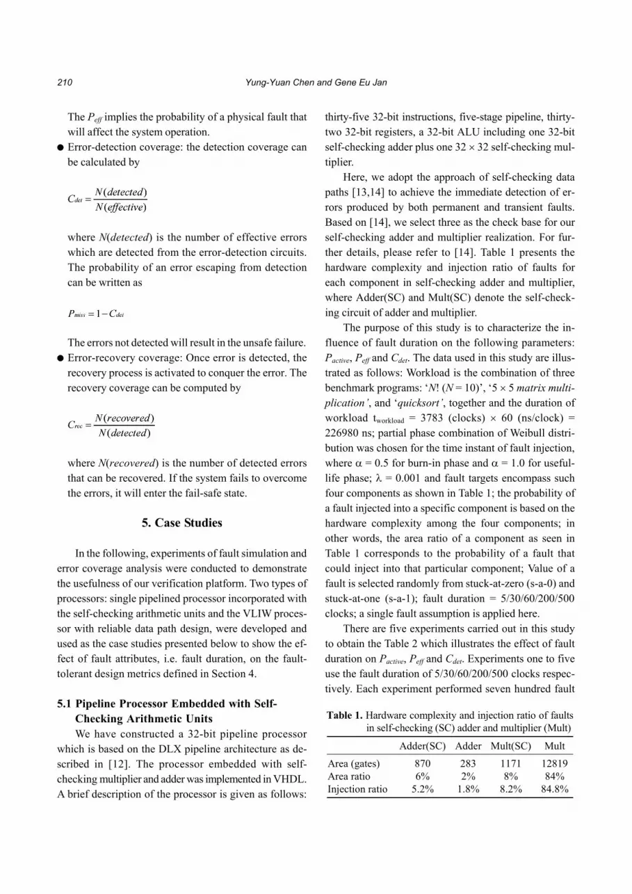
ther details, please refer to [14]. Table 1 presents the

hardware complexity and injection ratio of faults for

each component in self-checking adder and multiplier,

where Adder(SC) and Mult(SC) denote the self-check-

ing circuit of adder and multiplier.

The purpose of this study is to characterize the in-

fluence of fault duration on the following parameters:

Pactive, Peff and Cdet. The data used in this study are illus-

trated as follows: Workload is the combination of three

benchmark programs: ‘N� (N = 10)’, ‘5 � 5 matrix multi-

plication’, and ‘quicksort’, together and the duration of

workload tworkload = 3783 (clocks) � 60 (ns/clock) =

226980 ns; partial phase combination of Weibull distri-

bution was chosen for the time instant of fault injection,

where � = 0.5 for burn-in phase and � = 1.0 for useful-

life phase; � = 0.001 and fault targets encompass such

four components as shown in Table 1; the probability of

a fault injected into a specific component is based on the

hardware complexity among the four components; in

other words, the area ratio of a component as seen in

Table 1 corresponds to the probability of a fault that

could inject into that particular component; Value of a

fault is selected randomly from stuck-at-zero (s-a-0) and

stuck-at-one (s-a-1); fault duration = 5/30/60/200/500

clocks; a single fault assumption is applied here.

There are five experiments carried out in this study

to obtain the Table 2 which illustrates the effect of fault

duration on Pactive, Peff and Cdet. Experiments one to five

use the fault duration of 5/30/60/200/500 clocks respec-

tively. Each experiment performed seven hundred fault


Table 1. Hardware complexity and injection ratio of faults

in self-checking (SC) adder and multiplier (Mult)

Adder(SC) Adder Mult(SC) Mult

Area (gates) 870 283 1171 12819

Area ratio 6% 2% 8% 84%

Injection ratio 5.2% 1.8% 8.2% 84.8%

injection campaigns so as to guarantee the validity of the

statistical data obtained. Each injection campaign was

injected only a single fault so that we can easily examine

the outcomes of the injected fault. We use our fault injec-

tion tool based on the parameters described previously to

generate seven hundred faults within [0, tworkload]. Since

partial phase combination of Weibull distribution was

chosen for the time instant of fault injection, the distribu-

tion of seven hundred faults is 350 faults fall into the

burn-in phase [0, 56745 ns] and 350 faults into the use-

ful-life phase [56745, 226980 ns]. Each fault is then con-

tributed to a fault injection campaign. The injection ratio

of faults for each component is shown in Table 1 and

agrees well with the area ratio as expected.

With reference to Table 2, the Pactive and Peff increase

with an increase of fault duration, but the Cdet is almost

fixed irrespective of the fault duration. However, we

note that the Pactive increases slowly when fault duration

rises rapidly. From the simulation results, we observed

that the s-a-1 faults have higher probability to become

active than the s-a-0 faults since the bits of signals more

frequently contained the value zero than one. We also

know that the occurring probability of s-a-1 fault and

s-a-0 fault is equal. So, the 50% s-a-1 faults will be easy

to be active. Nevertheless, the 50% s-a-0 faults show

totally different feature. The probability of an s-a-0 fault

becoming active increases very slowly with increase of

the fault duration. It turns out that the Pactive increases

slowly when fault duration rises rapidly. As a result, the

efficiency of injection campaign is between 0.52 and

0.61 for the fault duration from five to five hundred clock

cycles. The Peff increases dramatically between five and

thirty clocks, and slows down the increase when fault

duration reaches two hundred clocks. The Peff results

indicate that the physical faults with short fault duration

(� 5 clocks) have low probability (� 0.31) to cause the er-

rors. For error-detection coverage Cdet, the self-checking

schemes can detect all single-bit faults except a situation

explained below. The self-checking multiplier cannot

detect a fault which occurs in multiplicand (or multi-

plicator), and meanwhile the multiplicator (or multipli-

cand) is a multiple of three. In the experiment of fault

duration being 30 clocks, one such situation happened

and the corresponding fault was never detected through-

out its effective duration. We discover that the occurring

probability of such situation is very low and approaches

to zero irrespective of the fault duration. If we assume

the inputs of multiplier are fault-free, then Cdet will be 1.0

as claimed by self-checking methodology.

5.2 VLIW Core with Reliable Data Path Design

A VLIW processor core with reliable data path design

devised by our team was employed here to explore the

concept of fault scenario furnished by our verification

platform. Figure 5 shows the architecture of our fault-tol-

erant VLIW core. In this case study, the original VLIW

core without fault-tolerant capability contains three ALUs

and three load/store units, and therefore, at most three

ALU instructions and three load/store instructions can be

issued concurrently per cycle. We note that the fourth

ALU as shown in Figure 5 is added for the purpose of as-

sisting the performing of error detection and error recov-

ery in error-handling process. So, this ALU is counted as

the extra cost paid to enhance the reliability of the data

paths. A32-bit ALU module includes a 32 � 32 multiplier.

With reference to Figure 5, the following notations are

used to explain the proposed error-handling scheme:

� TMR_MV(ALU_i, ALU_i+1, ALU_i+2): TMR_MV

is an abbreviation of Triple Modular Redundancy_

Majority Voter, which receives the outputs of ALU_i,

ALU_i+1 and ALU_i+2.

� r_no: Number of retries permitted for an incorrect in-

struction, where r_no > 0.

� CP1(ALU_1, ALU_2): CP is an abbreviation of Com-

Parator, which compares the outputs of ALU_1 and

ALU_2.

� CP2(ALU_3, ALU_4): ComParator2 is used to check

the outputs of ALU_3 and ALU_4.

The reliable data path design for ALU part is de-

scribed below:

Error-handling process:

while (not end of program)

{switch (number of ALU instructions in an

execution packet)

{case ‘1’: TMR_MV(ALU_1, ALU_2, ALU_3);


Table 2. The effect of fault duration on several parameters

duration 5 30 60 200 500

Pactive 0.52 0.5400 0.57 0.59 0.61

Peff 0.31 0.7200 0.79 0.88 0.89

Cdet 1.00 0.9963 1.00 1.00 1.00

if (TMR_MV detects more than one

ALU failure) then the “Error-recovery

process” is activated to recover the failed

instruction.

// if an execution packet contains only one ALU

instruction then it will be checked by Triple Mo-

dular Redundancy (TMR) scheme. //

case ‘2’: the execution packet contains two inst-

ructions: I1 and I2.

I1: CP1(ALU_1, ALU_2);

// instruction I1 executed with the compari-

son scheme using the ALU_1 and ALU_2. //

I2: CP2(ALU_3, ALU_4);

// instruction I2 executed with the compari-

son scheme using the ALU_3 and ALU_4. //

if (I1 fails) then the “Error-recovery pro-

cess” is activated to recover I1.

if (I2 fails) then the “Error-recovery pro-

cess” is activated to recover I2.

case ‘3’: Due to limited ALU resources, three con-

current ALU instructions cannot be all

checked at the same cycle by TMR and/or

comparison schemes. The three instruc-

tions need scheduling to two sequential

execution packets where one packet con-

tains two instructions and the other holds

the rest one; consequently, one extra ALU

cycle is required to complete the execu-

tion of three concurrent ALU instructions

for error-detection need. So, the packet is

divided to two packets and executed se-

quentially.

}}

Error-recovery process:

i � 1;

While (r_no > 0)


Figure 5. Architecture of fault-tolerant VLIW processor core.

{TMR_MV(ALU_i, ALU_i+1, ALU_i+2);

if (TMR_MV succeeds) then the error recovery

succeeds � exit;

else {r_no � r_no - 1; i � i + 1; if (i � 3) then i �

1;}}

Recovery fails and the system enters the fail-safe

state.

The VLIW core with reliable data path design based

on the features described previously was realized in

VHDL. In this experiment, we copied each of the follow-

ing benchmark programs: ‘N� (N = 10)’, ‘5 � 5 matrix

multiplication’, and ‘21

5

A Bi i

i

�

’, four times and then

the twelve programs were combined in random sequence

to form a workload for the fault simulation. The length of

workload is equal to 4384 (clocks) � 30 (ns/clock). The

injection targets in this experiment are confined to four

ALUs. Value of a fault was selected randomly from the

fault model depicted in Section 2.1. The settings of tool

parameters are described below: � = 1 (useful-life), fail-

ure rate (�) = 0.001, fault duration = 5/9/10/12/16/20

clock cycles. The number of retries r_no was set to two.

Next, we explain how to produce the different fault en-

vironments by varying the duration of faults injected

within the simulation campaigns.

Note that if simulation workload and fault-occurring

frequency are constants, the faults injected within the

simulation campaign with various fault durations will in-

fluence the degree of fault overlap. For instance, while

the duration of faults injected increases, the degree of

fault overlap will turn into more serious. In other words,

varying in duration of faults injected will lead to the dif-

ferent fault environments or fault scenarios. Six types of

injection campaigns varying in fault duration were set up

and the number of faults injected for each injection cam-

paign is fixed, namely 400. As the fault duration in-

creases, the degree of fault overlap will rise as well. Sta-

tistical data for six different fault scenarios using the

fault duration of 5, 9, 10 and 12, 16 and 20 clock cycles

respectively are illustrated in Table 3. Table 3 exhibits

the larger the fault duration, the worse the fault environ-

ment of the simulation campaign. While the duration of

injected faults increases, the probabilities of occurrence

of multiple faults and near-coincident faults rise too. The

simulation campaign with fault duration = 20 clock cy-

cles will lead to the worst fault scenario among six injec-

tion campaigns according to the data provided in Table 3.

Figure 6 shows the outcomes of the probability of er-

rors not detected, i.e. the probability of unsafe failure,

and the error-recovery coverage with different fault en-

vironments. Figure 6 reveals that the error-detection co-

verage and error-recover coverage of the system de-

crease as fault environment becomes worse. From Fig-

ure 6(a), the probability of unsafe failure increases from

0.0 to 0.0042, and error-detection coverage Cdet de-

creases from 1.0 down to 0.9958 as the fault duration is

from 5 to 20 clocks. The error-recovery coverage Crec as

indicated in Figure 6(b) decreases from 0.9991 down to

0.9801 as the fault duration is from 5 to 20 clocks.

Several notable observations are obtained from this

case study. One is the usefulness of the verification plat-

form which significantly enhances the efficiency and va-


Figure 6. Error coverage analysis. (a) probability of error not detected. (b) error-recovery coverage.

Table 3. Statistical data of each injection campaign

Fault duration

Pi (%)5 9 10 12 16 20

P1 81.47 67.58 64.49 57.70 43.94 33.72

P2 16.79 26.47 28.31 31.82 36.68 37.30

P3 01.63 05.22 06.51 09.01 15.90 21.28

P4 00.11 00.69 00.67 01.41 03.10 06.65

P5 00.04 00.02 00.04 00.29 00.95

P6 00.02 00.09 00.10

lidity of the dependability analysis. The results of statis-

tical analysis of each injection campaign help designers

build up a set of desired fault scenarios with different de-

grees of fault severity to verify the robustness of fault-

tolerant systems. As shown in this demonstration, six in-

jection campaigns with different fault activities were

chosen to be the test platforms for the system under vali-

dation. Consequently, we can easily realize how robust

of our system under a specific fault environment. It is

evident that our approach can facilitate us in gaining the

confidence of the experimental outcomes. Another is

that the results of error coverage are quite positive and

sound; those declare the feasibility of our fault-tolerant

scheme. It is worth noting that even in a very bad fault

environment, our system is still robust.

6. Conclusion

This paper presents a comprehensive verification

platform for dependability analysis of fault-tolerant sys-

tems. The verification platform encompasses the phases

of fault injection, simulation and data analysis. The pro-

posed fault injection tool can produce the diverse fault

scenarios which can be utilized to imitate the real fault

environments. Importantly, the fault-robust systems can

be examined under various fault environments to solidly

validate their capability of fault tolerance. Since fault-

tolerant systems are often used in critical applications,

validating such systems is imperative to guarantee the

dependability of the systems before they are being put to

use. Our tools fulfill this need substantially.

In the case studies, we have shown the influence of

fault duration and fault-occurring rate on the error cover-

age of the fault-tolerant processors. It is worth noting

that the system robustness is quite dependent on the fault

attributes such as fault duration, fault frequency and sin-

gle or multiple faults. The impact of various workloads

on dependability deserves to be investigated further.

References

[1] Clark, J. and Pradhan, D., “Fault Injection: A Method

for Validating Computer-System Dependability,” IEEE

Computer, Vol. 28, pp. 47�56 (1995).

[2] Hsueh, M. C., Tsai, T. K. and Iyer, R. K., “Fault Injec-

tion Techniques and Tools,” IEEE Computer, Vol. 30,

pp. 75�82 (1997).

[3] Fault Injection Techniques and Tools for Embedded

Systems Reliability Evaluation, edited by A. Benso

and P. Prinetto, Kluwer Academic Publishers (2003).

[4] Acle, J. P., Reorda, M. S. and Violante, M., “Early,

Accurate Dependability Analysis of CAN-Based Net-

worked Systems,” IEEE Design & Test of Computers,

pp. 38�45 (2006).

[5] Kanawati, G. A., Kanawati, N. A. and Abraham, J. A.,

“FERRARI: A Flexible Software-Based Fault and Er-

ror Injection System,” IEEE Trans. on Computers,

Vol. 44, pp. 248�260 (1995).

[6] Jenn, E., Arlat, J., Rimen, M., Ohlsson, J. and Karlsson,

J., “Fault Injection into VHDL Models: The MEFISTO

Tool,” FTCS-24, pp. 66�75 (1994).

[7] Folkesson, P., Svensson, S. and Karlsson, J., “A Com-

parison of Simulation-Based and Scan Chain Imple-

mented Fault Injection,” FTCS-28, pp. 284-293 (1998).

[8] Gil, D., Martínez, R., Busquets, J. V., Baraza, J. C. and

Gil, P. J., “Fault Injection into VHDL Models: Experi-

mental Validation of a Fault Tolerant Microcomputer

System,” EDCC-3, pp. 191�208 (1999).

[9] Tsai, T. K., Hsueh, M. C., Zhao, H., Kalbarczyk, Z. and

Iyer, R. K., “Stress-Based and Path-Based Fault Injec-

tion,” IEEE Trans. On Computers, Vol. 48, pp. 1183�

1201 (1999).

[10] Zarandi, H. R., Miremadi, S. G. and Ejlali, A., “De-

pendability Analysis Using a Fault Injection Tool

Based on Synthesizability of HDL Models,” 18th IEEE

International Symposium on Defect and Fault Toler-

ance in VLSI Systems, pp. 485�492 (2003).

[11] Siewiorek, D. P. and Swarz, R. S., Reliable Computer

Systems: Design and Evaluation, Burlington, MA: Di-

gital Press (1992).

[12] Hennessy, J. L. and Patterson, D. A., Computer Ar-

chitecture: A Quantitative Approach, San Mateo, CA:

Morgan Kaufmann (1996).

[13] Johnson, B. W., Design and Analysis of Fault Tolerant

Digital Systems, Reading, MA: Addison-Wesley (1989).

[14] Noufal, I. A. and Nicolaidis, M., “A CAD Framework

for Generating Self-Checking Multipliers Based on

Residue Codes Design,” Automation and Test in Eu-

rope Conference and Exhibition, pp. 122�129 (1999).

Manuscript Received: Sep. 14, 2007

Accepted: Jul. 15, 2009


Documents

Development of Scenario-Based Fault Injection Platform and Its Application Study