Forsch Ingenieurwes (2010) 74: 99–109DOI 10.1007/s10010-010-0119-y

O R I G I NA L A R B E I T E N / O R I G I NA L S

Vibrations of a vehicle excited by real road profiles

Marek Borowiec · Asok K. Sen · Grzegorz Litak ·Jacek Hunicz · Grzegorz Koszałka · Andrzej Niewczas

Received: 15 March 2010 / Published online: 30 April 2010© Springer-Verlag 2010

Abstract Based on experimental data obtained from theLublin III delivery car, we have performed a vibration anal-ysis of the vehicle suspension system. Vertical accelerationson the left and right sides of the suspension system weremeasured. Experiments were carried out on three types ofroad surfaces: (a) asphalt, (b) sett, and (c) railway cross. Theacceleration signals were examined using Fourier transform,multiscale entropy analysis and continuous wavelet trans-form. These methods reveal the characteristics of the vibra-tion patterns produced by the various road surface profiles.Our results can be used to assess the efficacy of a vehiclesuspension system under different road conditions.

Die durch reale Straßenprofile aufgeregtenSchwingungen eines Fahrzeuges

Zusammenfassung Der Lieferwagen Lublin III wurde ex-perimentell geprüft und aufgrund der so erhaltenen Datenwurde eine Schwingungsanalyse der Aufhängung des Fahr-zeuges durchgführt. Es wurden Beschleunigungen auf derlinken und rechten Seite der Aufhängung gemessen. Die Ex-perimente wurden auf der Straßendecke von verschiedenenProfilen durchgeführt: (a) Asphalt, (b) Pflasterwürfel, sowie

M. Borowiec · G. Litak (�)Department of Applied Mechanics, Technical Universityof Lublin, Nadbystrzycka 36, 20-618 Lublin, Polande-mail: g.litak@pollub.pl

A.K. SenDepartment of Mathematical Sciences, Indiana University, 402 N.Blackford Street, Indianapolis, IN 46202–3216, USA

J. Hunicz · G. Koszałka · A. NiewczasDepartment of Combustion Engines and Transport, LublinUniversity of Technology, Nadbystrzycka 36, 20-618 Lublin,Poland

(c) Bahnübergang. Beschleunigungssignale wurden mittelsFourier-Transformation, Multiskalen-Entropie-Analyse undkontinuierlicher Wavelt-Transformation geprüft. Diese Me-toden erlaubten die Charakteristik der Schwingungsmuster,die von den oben erwähnten verschiedenen Profilen der Stra-ßendecke erzeugt wurden, zu bekommen. Unsere Ergebnis-se können zur Bewertug der Wirksamkeit der Aufhängungeines Fahrzeuges in verschiedenen Straßenverhältnissen ver-wendet werden. Schlüssselwörter: Aufhängung, nichtlineareSchwingungen, Entropie, Walvet-Analyse.

List of symbolsa(i) Measured acceleration time series

(m/s2)i, j Time and frequency indicescj , sj Fourier coefficientsN Length of time seriesti Actual time (s)δt Sampling interval (s)Aj , A Fourier amplitude (m/s2)ωj Fourier frequencyf Vibration frequency (Hz)a

(τ)j Acceleration coarse-grained time

series (m/s2)a

(τ )i = a

(τ)i /σ (a(τ)) Normalized elements of

coarse-grained time seriesσ(a) Standard deviationr Similarity factorτ Scale factorMSE Multiscale entropyM Normalization factorpi(τ, r,m) Probability of finding the

coarse-grained sequence of the lengthm and the similarity r

AC(j) Autocorrelation function

100 Forsch Ingenieurwes (2010) 74: 99–109

W(s, τ ) Continuous wavelet transform (CWT)ψ(t), ψs,τ (t) Mother wavelet functionss, τ Scale and translation wavelet

parametersP(s, τ ) Wavelet power spectrumWn(s) Continuous wavelet transform of the

time seriesPn(s) Wavelet power spectrum of the time

seriesω0 Center wavelet frequencyW 2(s) Global power spectrum

1 Introduction

The effect of a rough road surface on vehicle vibrations, andin particular, on the driver and passengers is still a subjectof research among automotive manufacturers and researchgroups [1–10]. To better understand the behavior of differenttypes of vehicle suspensions, there are many tests carried outunder real road conditions. These tests are performed in or-der to identify and optimize the suspension parameters [11]and to minimize tire wear [12].

The relationship between anti-vibration performance andchaos characteristics of a vehicle suspension has been re-cently analyzed by Zhang and Ren [13]. Based on real ex-periments, several models have also been developed whichtake into account both the kinematic road curvature and/orinternal engine excitations [11, 14]. In addition, virtual testshave been proposed [15] to study the damping characteris-tics of the suspension system.

2 The experimental stand and the measurementprocedure

In this paper we report and subsequently analyze the mea-surement data from tests made on a delivery car suspen-sion. Experiments have been performed on the Lublin IIIcar manufactured by the polish industry “INTRALL PolskaS.A.” (Fig. 1). The test consists of simultaneous accelera-tion measurements of car vibrations on the left and rightsides of the front part of the suspension system under realdriving conditions. The accelerometers were mounted on thedown side denoted by point “B” (as an ‘unsprung mass’) andon the up side denoted by point “A” (as a ‘sprung mass’)with respect to the suspension column (Fig. 2a). We use theterms ‘unsprung’ and ‘sprung’ in the context of a quarter carmodel [3, 4] (Fig. 2b). Mounting the sensors in this specialway enabled us to test the suspension of the car more pre-cisely.

The piezoresistive accelerometers used for measurementshad sensitivity of about 1.02 mV/(m/s2), however each of

Fig. 1 An actual photo of the Lublin III vehicle

Fig. 2 A schematic diagram of the suspension column. The positionsof the acceleration sensors are indicated by A and B. The sensor sensi-tivity is 1.02 mV/(m/s2). (b) The quarter car model

them was calibrated by the manufacturer. They providedmeasurement range of ±4900 m/s2 with the resolution of0.1 m/s2 and non-linearity less than 1%. Thus, even at lowestaccelerations obtained at asphalt and 20 km/h resolution wasat least 20 times lower than measured peak signal. Althoughaccelerometers had some temperature sensitivity deviation(approx. 1%/50°C), in this experiment it can be omitted asmeasurements were done at almost constant ambient tem-perature. In the presented experiment, transverse sensitivityof the accelerometers can be a factor introducing some in-terferences into the signal. However, transverse sensitivity istypically less than 3%.

Accelerometers were excited with a constant currentsource built in an amplifier with a switchable gain from 1to 100. The amplifier output voltage signal was recordedwith the use of 12 bit resolution data acquisition system withsuccessive approximation A/D converter. During the experi-ments, the input voltage range of the data acquisition systemwas varied in order to fill the measurement range as much aspossible.

In order to avoid a time shift between consecutive mea-surement channels A/D, conversions were made in blocksconsisting of all input channels used. Blocks were triggered

Forsch Ingenieurwes (2010) 74: 99–109 101

Fig. 3 The data acquisitionsystem used in our experiment

with set sampling frequency 20 kHz or 50 kHz, while insidethe block consecutive channels were scanned with the con-stant period of 2 µs. Thus, data acquisition can be treated assimultaneous sampling.

The acceleration sensors were connected to a data acqui-sition module shown in Fig. 3. We were especially interestedin the frequencies and amplitudes of the car vibration sig-nals measured directly on the wheel axes and after passingthrough the damper. The car was excited kinematically byroad roughness. During the test we used different road sur-faces, i.e., asphalt, sett and railway track cross. The featuresof a road profile based on sett and a railway crossing arepresented in detail in Fig. 4.

The accelerations were measured in voltage units [mV],with 10 mV gauged as the standard gravitational accelera-tion g. In Fig. 5 we have plotted the time series of the ac-celeration measurements where the car velocity was main-tained constant at 20 km/h. From this figure one can eas-ily see that some level of noise is present in all investigatedcases. Note that the acceleration time series for the ‘sprung’and ‘unsprung’ masses are plotted on different scales. Wehave calculated the standard deviations σ for the varioustime series and obtained the following results: (Fig. 5a) 1.47,(Fig. 5b) 1.30, (Fig. 5c) 5.14, (Fig. 5d) 2.94. Comparing thestandard deviations for the ‘unsprung’ and ‘sprung’ masses,it is clear that the vibrations are damped effectively afterpassing through the damper. Furthermore, the results for σ

and also visual inspection of Figs. 5a–b and Figs. 5c–d re-veal that the asphalt road surface provides weaker excita-tion to the car than the sett surface as we expected. A simi-lar effect of lowering in the level of vibration while passingthrough the damper is also visible for the railway road crossin Figs. 5e–f.

To determine the distribution of harmonics in the acceler-ation signals (Figs. 5a–d), we have calculated their discrete

Fig. 4 Features of the road surface profile used in our experiment:(a) sett, and (b) railway cross. The dimensions are in millimeters

Fourier transform. For the signal a(i), where i denotes thetime index, we write

cj = 2

N

N∑

i=1

a(i) cos(iωj ),

sj = 2

N

N∑

i=1

a(i) sin(iωj ).

(1)

Note that the actual time ti = i(δt), δt being the sam-pling interval. Here the amplitude Aj and frequency ωj aredefined respectively as

Aj =√

c2j + s2

j , ωj = 2πj

N. (2)

102 Forsch Ingenieurwes (2010) 74: 99–109

Fig. 5 Time series of the acceleration signals measured from theleft side of the car suspension for different types of road surface:(a) & (b) asphalt, (c) & (d) sett, and (e) & (f) railway cross. The fig-ures (a), (c) and (e) are for ‘unsprung’ mass, whereas the figures (b),(d) and (f) are for ‘sprung’ mass. These measurements were made with

the car running at 20 km/h. Note that the sampling rate used for thetime series of asphalt and sett surfaces [(a)–(d)] is 50 kHz, whereas asampling rate of 20 kHz is used for the time series of railway crossingsurface shown in (e) & (f)

See [16] for details. Figs. 6a and b present plots of theFourier transforms for asphalt and sett surfaces, respectively,with the car running at 20 km/h. Generally the responseof the vehicle subjected to the sett type of road profile isstronger. This is to be expected because this type of road sur-face possesses more corrugations in its profile. In the Fourierspectra we see clear peaks suggesting resonant responses. Itappears that their origins have various sources. In Fig. 6aand b we have shown several significant areas of frequen-cies marked by numbers ‘1’, ‘2’, ‘3’, and ‘4’. The ranges inthe vicinity of 1 Hz and 15 Hz marked by ‘1’ and ‘2’ denotethe main frequencies of free vibration of the vehicle suspen-sion. Note that our physical model, based on unsprung andsprung masses (Fig. 2b), has two degrees of freedom. Re-gion ‘3’ in Fig. 6a may reflect that the real vehicle system

has more degrees of freedom [9]. In Fig. 6a and Fig. 6b (notea different vertical scale in Fig. 6a and b) one can see ad-ditional peaks outside 1000 Hz denoted by ‘4’ are far awayfrom what you can expect to describe by simple rigid bodymodels of a wheel suspension.

Note that the sampling rate was 10 orders of magnitudehigher than that resulting from the Nyquist criterion [16].However, the maximum frequency of sensor response isknown to be 10–90% of the measurement range. At smalleramplitudes the time response of the sensor can be shorter.In order to analyze the existence of a frequency band andits shape, the sampling frequency was increased. Further-more, as the natural frequency of the sensor is about 12 kHz,smaller sampling rates allow to identify particular peaks ofamplitudes in the frequency bands.

Forsch Ingenieurwes (2010) 74: 99–109 103

Fig. 6 Fourier transforms of the measured acceleration signals at thecar velocity of 20 km/h. Note that a logarithmic scale is used for fre-quency

3 Multiscale entropy analysis

Many physical systems evolve on multiple time scales andexhibit complex dynamics [17–20]. In recent years there hasbeen a great deal of interest in quantifying the complexityof these systems. Analysis of these multiscale systems usingmethods based on a single scale is inappropriate and maylead to erroneous results. To describe complexity in an ac-curate manner, the different time scales should be taken intoaccount. Recently Costa et al. [21] introduced the conceptof multiscale entropy (MSE) to quantify the complexity ofsuch multiscale systems. This concept was used to describethe nature of complexity in physiological time series suchas those associated with cardiac dynamics [22] and gait me-chanics [23]. In this paper we perform a multiscale entropyanalysis as a measure of complexity of the vehicle system.MSE is based on a coarse-graining procedure and can becarried out on the time series of ‘unsprung’ and ‘sprung’masses.

For multiscale entropy analysis we scale the time seriesas follows. For a given time series {a1, a2, . . . , an}, whereai = a(i), we construct multiple coarse-grained time seriesby averaging the data points within non-overlapping win-dows of increasing length as shown in Fig. 7:

a(τ)j = 1

τ

jτ∑

i=(j−1)τ+1

ai, (3)

Fig. 7 Scheme of the coarse-graining procedure used in the calcula-tion of multiscale entropy (MSE)

where τ represents the scale factor, and 1 ≤ j ≤ N/τ , withthe length of each coarse-grained time series being equal toN/τ . Note that for τ = 1, the coarse-grained time series issimply the original time series. Using these coarse-grainedtime series, the MSE can be defined in terms of Shannoninformation entropy as follows:

MSE = − 1

M

∑

i

pi(τ, r,m) lnpi(τ, r,m). (4)

Here M is a normalization factor, pi(τ, r,m) is the prob-ability of finding the coarse-grained sequence of a

(τ )i of

m is the length of a measurement sequence, and r de-notes a similarity factor defined to identify two measuredpoint values (a(i), a(j)) if their difference �a(τ) is smallerthan r :

r > �a(τ). (5)

The quantity a(τ )i is a

(τ)i normalized by the corresponding

standard deviation a(τ )i = a

(τ)i /σ (a(τ)). In our calculations

we have used m = 3 and r = 0.15.The multiscale entropies for the ‘unsprung’ and ‘sprung’

masses are presented in Fig. 8 for the three types of roadsurfaces considered here. In each figure, the colors red andgreen correspond to ‘unsprung’ and ‘sprung’ masses. re-spectively. For comparison, a horizontal line in these figurescharacterizes 1/f type or pink noise, which frequently arisesin biological systems such as DNA sequences and heartbeattime series. On the other hand, a hyperbolic curve indicatesthe presence of Gaussian white noise.

Traces of these characteristic behaviors can be foundin our results for different scale factors τ . For example,in Fig. 8a (red and green lines) and Fig. 8b (red line)one can find elements of white noise in the vehicle vibra-tion, but in Fig. 8c (red and green line) and in Fig. 8b(green line), the vibrations are of 1/f type. Note thatfor smaller τ the entropy increases in all figures. Thelinear-like increase could be associated with the correla-tions between measured neighboring points. For clarity we

104 Forsch Ingenieurwes (2010) 74: 99–109

Fig. 8 (Color online) MSE plots of the various acceleration time seriesfor the car velocity of 20 km/h. The values of the pattern length m = 3and similarity factor r = 0.2 are used. The colors green and red applyto ‘sprung’ and ‘unsprung’ masses, respectively

have plotted the corresponding autocorrelation functions inFigs. 9a–f.

The autocorrelation function AC(j) is a convolution ofthe acceleration time series ai , and is given by:

AC(j) =∑

i

aiai+j , (6)

with appropriate normalization to one.All the figures (Figs. 9a–f) indicate that neighboring

points of the signals are highly correlated. Note that in

Figs. 9a, c and d, AC is going to 0 for j = jc where jc �1000. In Fig. 9b, jc ≈ 150.

In Figs. 9e–f, where the sampling rate was different fromthe other cases, one can also see strong correlation betweenneighboring points leading to a similar tendency for smallscaling factors (Fig. 8c).

Interestingly, in all plots (Figs. 8a–c) the entropy of the‘sprung mass’ is larger than that of the ‘unsprung mass’, in-dicating a more regular motion of ‘unsprung mass’. On theother hand, values of the standard deviations indicate thatthe amplitude of vibration of the ‘sprung mass’ is smallerthan that of the ‘unsprung mass’. These are typical rela-tions that one can expect from the correctly working sus-pension of a vehicle which filters out selected harmonics.In other words, the ‘sprung mass’ oscillations can be re-lated to the noisy background of the ‘unsprung mass’ mo-tion.

We should also remark that in case of the sett road sur-face, there is a clear variation in the characteristics of thenoise measured by MSE. For relatively small scale factorsτ ∈ [10,25], the ‘sprung’ mass follows the white noise char-acteristics, whereas for larger value of τ > 25 the character-istics of pink noise (1/f ) are identified. This can be relatedto the interaction between the effect of deformation of thetire and the response of the vehicle suspension while cross-ing a single obstruction. The appearance of pink noise withhorizontal lines in Figs. 8a, b may be associated with fractalphenomena [34]. It can mimic the scaling properties of realroad roughness or a complex system response for chaoticmotion. In the case of crossing railway track, the MSE re-sult depends on contributions from different qualities of sur-faces, which in effect gives a flat characteristic shape seenin Fig. 8c.

4 Wavelet analysis

In this section we perform a wavelet analysis of the variousacceleration time series, a(t), using a continuous wavelettransform (CWT). Wavelets have been used in diverse ap-plications including dynamic analysis of structural systems[24–33]. First, we briefly describe the procedure of CWT.A continuous wavelet transform W(s, τ ) of a function a(t)

with respect to a mother wavelet ψ(t), is defined as the con-volution of the function with a scaled and translated versionof the mother wavelet:

W(s, τ ) =∫ ∞

−∞a(t)ψ∗

s,τ (t)dt, (7)

where

ψ∗s,τ (t) = 1√

sψ∗

(t − τ

s

). (8)

Forsch Ingenieurwes (2010) 74: 99–109 105

Fig. 9 Autocorrelation functions of the acceleration time series for different types of road surfaces: (a) & (b) asphalt, (c) & (d) sett, and(e) & (f) railway cross. (a), (c) and (e) are for ‘unsprung’ mass, whereas the figures (b), (d) and (f) are for ‘sprung’ mass

The symbols s and τ represent the scale and translation pa-rameters, respectively. The asterisk in Eq. 7 denotes a com-plex conjugate. The scale parameter controls the dilationwhereas the translation parameter indicates the location ofthe wavelet in time. The mother wavelet satisfies the condi-tions:∫ ∞

−∞ψ(t)dt = 0,

∫ ∞

−∞|ψ(t)|2dt < ∞. (9)

The wavelet power spectrum P(s, τ ) of the signal a(t) isdefined as the squared modulus:

P(s, τ ) = |W(s, τ )|2 . (10)

In the case of a signal a(t) described by a time series

a(t) → ai, i = 1,2, . . . ,N, (11)

a discretized version of Eq. 7 should be used. Following Tor-rence and Compo [30], we may write:

Wn(s) =N∑

n′=0

(δτ

s

)an′ψ∗

[(n − n′)δτ

s

], (12)

where n is the time index and δτ is the sampling interval.The corresponding power spectrum is given by:

Pn(s) = |Wn(s)|2 . (13)

In our analysis we used a Morlet wavelet as the motherwavelet. A Morlet wavelet consists of a plane wave mod-ulated by a Gaussian function and is described by:

ψ(η) = π−1/4eiω0ηe−η2/2, (14)

106 Forsch Ingenieurwes (2010) 74: 99–109

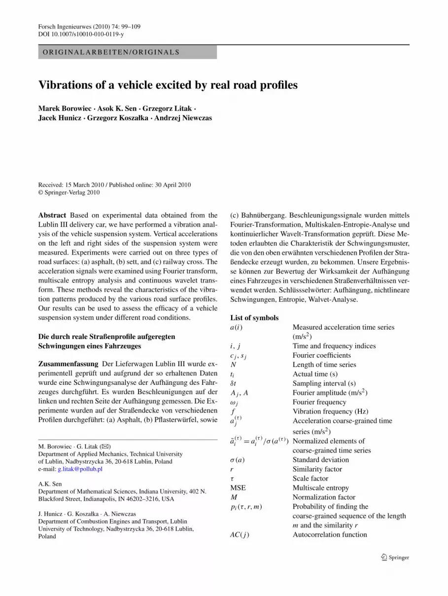
Fig. 10 Results of wavelet analysis for different road surfaces: (a) & (b) asphalt, (c) & (d) sett, and (e) & (f) railway cross. (a), (c) and (e) are for‘unsprung’ mass, whereas the figures (b), (d) and (f) are for ‘sprung’ mass

where ω0 is the center frequency, also referred to as the orderof the wavelet. Morlet wavelets have been used in a wide va-riety of applications for feature extraction in time series data.We have used a Morlet wavelet with ω0 = 6 in all our cal-culations. This choice of ω0 offers a good balance betweentime and frequency localizations.

From the wavelet power spectrum (WPS) which is localin nature, a global wavelet spectrum (GWS) can be calcu-

lated by averaging the WPS over the entire time interval.The GWS is given by:

W 2(s) = 1

N

N∑

n=1

|Wn(s)|2 . (15)

(See [30] for details.) The GWS is similar to the smoothedFourier power spectrum. From the locations of the peaks in

Forsch Ingenieurwes (2010) 74: 99–109 107

Fig. 10 (Continued)

the GWS, the most dominant periods (or frequencies) in atime series can be readily identified.

The wavelet power spectrum as given by Eq. 9 dependson scale and time, and is sometimes referred to as a scalo-gram. The scalograms for the ‘sprung’ and ‘unsprung’ sidesare depicted in Fig. 10 for the three types of road surfacesexamined here. Figures 10a, b apply to the asphalt surface,Figs. 10c, d apply to the sett surface, whereas Figs. 10e, fare for the railway cross track. The global wavelet spectra

(GWS) for the different cases are shown on the right sidesof the scalograms. In Fig. 10, comparison of each pair offigures, namely, (a, b), (c, d), and (e, f), reveals that for eachtype of road surface, the dominant frequency on the ‘sprungmass’ side is lower than that on the ‘unsprung mass’ side,as one would expect. The presence of intermitency at higherfrequencies (i.e., at smaller scales) is also apparent in thesefigures.

In the case of crossing by a railway track one can clearlysee excitations grouped in pairs of impulses. Interestingly,the time scale of excited vibrations is different for ‘sprung’and ‘unsprung’ masses. In fact, the ‘unsprung mass’ excita-tion is disappearing relatively faster compared to the ‘sprungmass’ for which the system response is more complex and isassociated with an additional shift of the period into smallervalues (higher frequencies).

5 Discussion of results and conclusions

By analyzing the acceleration signals we have studied thevibration characteristics of the suspension system of theLublin III delivery car subjected to rough road kinematicexcitations. In addition to the standard Fourier analysis, wehave used the methods of multiscale entropy analysis andcontinuous wavelet transform. The accelerations were mea-sured on both the down (unsprung mass) and the up (sprungmass) sides of the suspension column. Three different typesof road surfaces were examined: asphalt, sett and cross byrailway track.

Our results may be summarized as follows. First, Fourieranalysis of the signals clearly indicates that our system hastwo spectral maxima. Second, the car suspension works asa low–pass filter decreasing more efficiently the amplitudesat higher frequencies. Third, the multiscale entropy analy-sis revealed the scaling features of the vibrations. Note thatthe entropy calculated for the ‘sprung mass’ was higher thanthat for the ‘unsprung mass’, whereas the standard devia-tions σ(a) behaved in the opposite way:

MSE(a, ‘sprung’) > MSE(a, ‘unsprung’),

σ (a, ‘sprung’) < σ(a, ‘unsprung’).(16)

This implies that the signal generated by a rough road sur-face after passing through the suspension is more noisy. Ev-idently the vehicle suspension reduces the vibrations in a se-lective way. This conclusion was also confirmed by waveletanalysis. Comparing the corresponding spectra (Figs. 6a–d)and their means for ‘sprung’ and ‘unsprung’ masses, onecan see clearly that some smaller periods (higher frequen-cies) are eliminated more easily. Interestingly, as a resultof this filtering, the spectra are changed from the originaltwo dominated frequencies into a single frequency. To ex-amine this effect in detail, we need to examine the results

108 Forsch Ingenieurwes (2010) 74: 99–109

Fig. 11 Fourier transforms of the measured signals for the ‘unsprung’and ‘sprung’ mass with the car running at 20–80 km/h for differentroad surfaces: (a) & (b) road asphalt, (c) & (d) sett. Note that, as inFig. 6, a logarithmic scale is used for frequency

for different car velocities. In Fig. 11, we have plotted theFourier transforms of the measured signals with car veloci-ties of 20–80 km/h for the ‘unsprung’ and ‘sprung’ masses,

and for two different road surfaces: Figs. 11a–b for asphalt,and Figs. 11c–d for sett. One can observe the rise in am-plitude when the vehicle is driven at a higher velocity, butthe regions of important frequencies are the same. Some no-ticeable increases in the region of 50–100 Hz (especially fora sett road) can indicate that higher frequency excitationsfrom the road profile are more important at higher velocities.This is more evident for the ‘unsprung mass’ (Figs. 11a, c)than for the ‘sprung mass’ where the higher frequencies arestrongly damped. Note that for all the velocities the responseof the vehicle subjected to the sett type of a road profile isstronger. The general conclusion is that the case of veloc-ity 20 km/h is a typical one and we claim that our resultsdiscussed for this velocity are relevant for a wider range ofvelocities.

Note also that the presence of short harmonics in thewavelet power spectra (Fig. 10) shows an evidence of in-termittent behavior in vehicle vibrations. The driving teststhrough the railway cross show non-stationary motion ofthe corresponding ‘sprung’ and ‘unsprung’ masses. The flatshape in entropy indicates (Fig. 8) that the overall contribu-tion of frequencies is coming in nontrivial way of pink noiseappearing in the context of chaotic dynamics. Here it canreveal the wide range of roughness changes present duringcrossing the railway track.

6 Final remarks

The present analysis was based on a real vehicle and in realroad conditions measurements. The results were discussedusing the 2 DOF model with single ‘unsprung’ and ‘sprung’masses by limiting discussion to the single side of the frontsuspension. This was a strong simplification because thepresent car had a dependent suspension in the front part. Themore accurate analysis would include the four wheels inde-pendent sensors, full car dynamics, and multivariant analy-sis [9]. We plan to perform such analysis as a continuationof the present study.

The effects of tires were of less importance as the pneu-matic tire structure can be treated as a linear system [35]with the vibration amplitude response proportional to theexcitation force. Considering the diameter (16′′) and the ra-dial structure of used tires, according to [36], the naturalfrequency of such a tire is about 100 Hz and damping ra-tio calculated as the rate of a logarithmic decrement is atlevel of 0.03. The natural frequency of the tire structure canbe noticed at Fourier transforms (Fig. 6) at point denotedas 3. Both mentioned values are practically independent ofvehicle speed, however strongly influenced by inflation pres-sure [36]. During the experiments tire pressure was constantand set to values recommended by the car manufacturer.

Forsch Ingenieurwes (2010) 74: 99–109 109

Acknowledgements The authors would like to thank Prof. KrzysztofŁukasik and Dr. Rafał Longwic for useful discussions and the PolishMinistry of Science and Higher Education for partial support (No.NN50204832/3680 and NN501007033).

References

1. Mitschke M (1990) Dynamik der Kraftfahrzeuge. Springer, Berlin2. Andrzejewski R, Awrejcewicz J (2005) Nonlinear dynamics of a

wheeled vehicle. Springer, New York3. Verros G, Natsiavas S, Papadimitriou C (2005) Design optimiza-

tion of quarter-car models with passive and semi-active suspen-sions under random road excitation. J Vib Control 11:581–606

4. Von Wagner U (2004) On non-linear stochastic dynamics of quar-ter car models. Int J Non-Linear Mech 39:753–765

5. Turkay S, Akcay H (2005) A study of random vibration character-istics of the quarter-car model. J Sound Vib 282:111–124

6. Verros G, Natsiavias S, Stepan G (2000) Control and dynamics ofquarter–car models with dual-rate damping. J Vib Control 6:1045–1063

7. Litak G, Borowiec M, Friswell MI, Szabelski K (2008) Chaoticvibration of a quarter-car model excited by the road surface profile.Commun Nonlinear Sci Numer Simul 13:1373–1383

8. Borowiec M, Litak G, Friswell MI (2006) Nonlinear response ofan oscillator with a magneto-rheological damper subjected to ex-ternal forcing. Appl Mech Mater 5–6:277–284

9. Zhu Q, Ishitobi M (2006) Chaotic vibration of a nonlinear full-vehicle model. Int J Solids Struct 43:747–759

10. Zhu Q, Ishitobi M (2004) Chaos and bifurcations in a nonlinearvehicle model. J Sound Vib 275:1136–1146

11. Lee J, Thompson DJ, Yoo HH, Lee JM (2000) Vibration analy-sis of a vehicle body and suspension system using a substructuresynthesis method. Int J Veh Des 24:360–371

12. Braghin F, Cheli F, Melzi S, Resta F (2006) Tyre wear model:validation and sensitivity analysis. Meccanica 41:143

13. Zhang Y, Ren C (2006) Test analysis on relationship between anti-vibration performance and chaos characteristics of vehicle suspen-sion. J Southeast Univ 22:64–68

14. Xuebao ZG (2006) Experimental and calculation methods for de-termining damping properties of the inertia track in a hydraulicengine mount. J Vib Eng 19:376–381

15. Huizinga ATMJM, Van Ostaijen MAA, Van Oosten SlingelandGL (2002) A practical approach to virtual testing in automotiveengineering. J Eng Des 13:33–47

16. Oppenheim AV, Schafer RW, Buck JR (1999) Discrete-time signalprocessing. Prentice Hall, New Jersey

17. Litak G, Kaminski T, Czarnigowski J, Sen AK, Wendeker M(2009) Combustion process in a spark ignition engine: analysisof cyclic maximum pressure and peak pressure angle oscillations.Meccanica 44:1–11

18. Grassberger P (1991) In: Atmanspacher H, Scheingraber H (eds)Information dynamics. Plenum, New York

19. Imponente G (2004) Complex dynamics of the biological rhythms:Gallbladder and heart cases. Physica A 338:277–281

20. Strozzi F, Zaldivar JM, Zbilut JP (2007) Recurrence quantifica-tion analysis and state space divergence reconstruction for finan-cial time series analysis. Physica A 376:487–499

21. Costa M, Goldberger AL, Peng C-K (2002) Multiscale analysis ofcomplex biological signals. Phys Rev Lett 89:068102

22. Costa M, Goldberger AL, Peng C-K (2005) Multiscale analysis ofbiological signals. Phys Rev E 89:021906

23. Costa M, Peng C-K, Goldberger AL (2003) Multiscale analysis ofhuman gait dynamics. Physica A 330:53–60

24. Kumar P, Foufoula-Greorgiou E (1997) Wavelet analysis for geo-physical applications. Rev Geophys 35:385–412

25. Gencay R, Selcuk F, Whitcher B (2001) An introduction towavelets and other filtering methods in finance and economics.Academic Press, London

26. Akay M (1997) Time-Frequency and Wavelets in Biomedical Sig-nal Processing. Wiley, New York

27. Ozguc A, Atac T, Rybak J (2003) Temporal variability of the flareindex (1966–2001). Sol Phys 214:375–397

28. Staszewski WJ, Worden K (1999) Wavelet analysis of time series:coherent structure, chaos and noise. Int J Bifurc Chaos 9:455–471

29. Wong LA, Chen JC (2001) Nonlinear and chaotic behavior ofstructural systems investigated by wavelet transform techniques.Int J Non-Linear Mech 36:221–235

30. Torrence C, Compo GP (1998) A practical guide to wavelet anal-ysis. Bull Am Meteorol Soc 79:61–78

31. Sen AK, Litak G, Taccani R, Radu R (2008) Wavelet analysis ofcycle-to-cycle pressure variations in an internal combustion en-gine. Chaos Solitons Fractals 38:886–893

32. Sen AK, Longwic R, Litak G, Górski K (2008) Cycle-to-cyclepressure oscillations in a diesel engine. Mech Syst Signal Process22:362–373

33. Longwic R, Litak G, Sen AK (2009) Recurrence plots for dieselengine variability tests. Z Naturforsch 64:96–102

34. Mandelbrot B (1977) Fractals: form, chance and dimension. Free-man, San Francisco

35. Genga Z, Popov AA, Cole DJ (2007) Measurement, identifica-tion and modelling of damping in pneumatic tyres. Int J Mech Sci49:1077–1094

36. Kim BS, Chi CH, Lee TK (2007) A study on radial directionalnatural frequency and damping ratio in a vehicle tire. Appl Acoust68:538–556