Differential Restrictions Applied to Pollutant Dispersion

Differential Restrictions Applied to Pollutant Dispersion

Jorge R. Zabadal, Vinicius G. Ribeiro, Cristiana A. Poffal

Abstract - Atmospheric pollution can be harmful to people’s health, especially in urban areas and close to chemical industries. In order to prevent and minimize the environmental impacts from these industries, it is convenient to use computational systems that simulate scenarios related to pollutant dispersion. In this work, a new analytical method is proposed to solve the correspondent mathematical model. The method uses two first order differential restrictions, which produce auto-Bäcklund transformations to the steady two dimensional advection diffusion equation. The main feature of this formulation is that the processing time to obtain the analytical solutions is significantly reduced.

Keywords—Pollutant dispersion, Advection-diffusion equation, Exact solutions, Bäcklund transformations.

I. INTRODUCTION

In order to estimate the environmental damages caused by the emission of gas effluent from chemical industries, it is necessary to simulate several possibilities associated to theeffluent level and type of treatment to be employed in the process. The simulation of different scenarios allows the alternatives’ evaluation to minimize the environmental damage, also considering the cost related to each of them. The aim of minimizing the environmental damage is to keep the pollutant concentration under the values defined by the environmental rules.

The simulations of these scenarios use mathematical models based on maps and tables which present the pollutantconcentration distribution close to the source. These models describe boundary problems based on the advective diffusive equation applied to atmospheric pollutant dispersion. Simulating several scenarios in order to choose the best alternative to the project requires resolution methods with the following features:

- low processing time; - the possibility of simulating dispersion in subdomains

with variable spatial resolution; - flexibility related to the region topography and to the

prescribed boundary conditions. The best treatment choice of the gas effluents from an

industry which is causing atmospheric pollution should minimize the environmental damage, obeys the environmental rules and requires a steady-state model in order to simulate typical scenarios.

Another important problem in environmental engineering is the accidental gas discharge, as a consequence of a serious accident during the productive process. In this situation, the existence of an instantaneous discharge yields a transient problem whose solution can be obtained via methods which allow analyzingthe pollutant spatial and time distribution. In this case, the low processing time is a viability criterion, as deciding whether or not taking steps in order to minimize the environmental damage must be performed in a short period of time. It is important to verify if it necessary to advise the population about risks, to make people leave their houses, stores or industries immediately. All these options are based on the scenarios that describe the plume dispersion.

At this point, it is important to mention that most of the methods employed to solve atmospherical pollution problems use the Gaussian Plume model. This model considers the pollutant plumes travel downwind when rising its source – the wind velocity is considered constant and uniform – which determines the main directions of the plumes’ path through the atmosphere [1][2].

In this model some hypothesis are performed in order to simplify the solutions field of the advective diffusion equation in its original form:

The components of the velocity vector are considered constant and uniform, that is, they do not depend on time or space;

The diffusive model is linear, neglecting the important effect of anomalous diffusion;

The environment is considered infinity, so only second kind boundary conditions are applied close to soil.

In this paper, it is proposed a pollutant propagation model based on a factorization of the advective diffusion equation, producing two first order partial differential equations. This model allows considering the nonlinearity that arises from the dependence of the diffusivity on the concentration and possible anisotropic terms that result from the dependenceon temperature.

The main advantage of using this factorized form is the fact that future implementationsor changes in the correspondent resolution method are not necessary, on the contrary that occurs with the original form of second order advection diffusion equation. This implies directly in four operational advantages:

- a compact source code which allows simple depuration; - high performance of the resolution method based on the

symbolic process;

INTERNATIONAL JOURNAL OF MATHEMATICAL MODELS AND METHODS IN APPLIED SCIENCES Volume 8, 2014

ISSN: 1998-0140 233

- the analytic character of the obtained solution makes easy the physical interpretation of the phenomenon occurred on the simulated scenarios. Besides, it allows the application of several sensibility tests related to the thermodynamic variables, such as temperature and pressure, without a great computational effort;

- as temperature and pressure can appear explicitly on the resultant solution, at first it is not necessary to divide the domain according to the planetary boundary layer features.

The advection diffusion equation can be solved by numerical, analytical and hybrid methods [3], but the analytical solution for some problems of great interest in environmental engineering is not already known.Analytical solutions have several advantages: they are expressedin a closedform; the computational codes based on these kinds of solutions require less processing time, since there is a reduction of the number of operations to be performed, and then the amount of memory required to execute the routines decreases significantly. Besides, the source codes based on closed-form solutions are short and easy to depurate.

The main numerical methods applied to solve the advection diffusion equation are based on discrete formulations, such as finite difference and finite elements, or spectral methods. It is possible to compare these methods features by listing their advantages and limitations when used to solve the proposed problem.

The finite difference method requires a great computational effort to solve multidimensional transient problems. It is a consequence of the discretization scheme needed close to interfaces or in regions where high concentration, temperature or pressure gradients occur. The use of variable mesh density [4] or employing curvilinear coordinates to adapt the boundary geometry [5]-[7] are some of the alternatives used to reduce the computational processing time of this method.

Systems based on finite elements are versatile to represent complex geometries because they have specialized generators of triangular and hexagonal grids that can be adapted to the region geometry. They also allow variable size to each element that composes the mesh and the boundary conditions can be easily applied [8]-[10]. However, to two dimensional problems, yield high order algebraic systems.

In order to combine the numerical methods versatility and the computational performance of the analytical formulations, exact solutions valid in wide subdomains can be applied. These solutions have a sufficient number of arbitrary constants to preserve the spatial resolution of the concentration maps and speed, without employing source codes that need high processing time. It happens because the algebraic systems resultant from the imposition of solution continuity over sub domains interfaces and the application of low order boundary conditions can be decoupled.

These solutions can be obtained by hybrid formulations which search for particular solutions, and not the general ones, as the traditional analytical methods. The latter would be very restricted to describe a great number of scenarios, but when using symbolic computation, they are easy and fast applied. Such programs, developed in last two decades, are making

possible the use of analytical tools in problems in which solving by traditional numerical methods would be very onerous [11].

These analytical tools are extremely helpful to solve nonlinear partial differential equations.They arise from methods based on the application of symmetries and mappings [12]-[14], as well as commutation relations [15]-[18].

There are partial differential equations whose factored forms obtained via order reduction yield solutions containing not only arbitrary constants, but also arbitrary functions of one or more variables[19]-[20]. These solutions are especially advantageous from the computational point of view, because they are usually described by compact expressions. So, they facilitate the boundary conditions application.

The aim of this paper is a new analytical method is proposed to solve the mathematical model which describes the pollutant dispersion in atmosphere. The method uses two first order differential restrictions, which produce auto-Bäcklund transformations to the advective diffusive two-dimensional steady equation.

This article is outlined as follows. In section 2, methodology and results are presented. In section 3, conclusion and recommendations for future work are drawn.

II. METHODOLOGY AND RESULTS

The advection diffusion equation which describes the

pollutant dispersion in the atmosphere is

2 2

2 2

C C C Cu v Dx y x x

∂ ∂ ∂ ∂+ = + ∂ ∂ ∂ ∂

, (1)

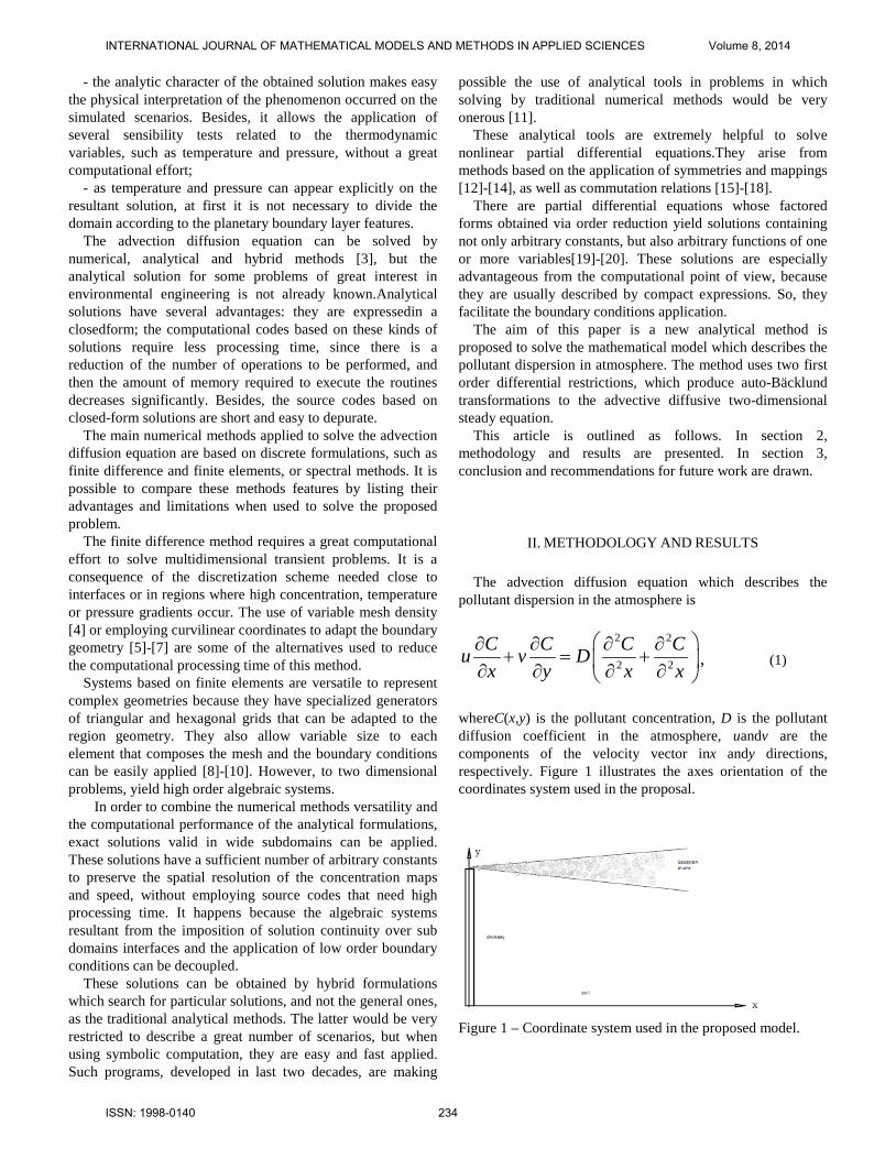
whereC(x,y) is the pollutant concentration, D is the pollutant diffusion coefficient in the atmosphere, uandv are the components of the velocity vector inx andy directions, respectively. Figure 1 illustrates the axes orientation of the coordinates system used in the proposal.

Figure 1 – Coordinate system used in the proposed model.


ISSN: 1998-0140 234

Equation (1) can be factored as:

C au C Dx y

∂ ∂= +

∂ ∂ (2)

and

,C avC Dy x

∂ ∂= −

∂ ∂ (3)

where ( )yxa , is an arbitrary function which belongs to the

null space of the divergent operator. The application of thedivergent over the system represented by the system formed by (2) e (3), i.e., the sumof the expressions obtained by the partial derivation, yields:

2 2

2 2,

C C u vu v Cx y x y

C CDx y

∂ ∂ ∂ ∂+ + + = ∂ ∂ ∂ ∂

∂ ∂+ ∂ ∂

(4)

which is an advection diffusion equation with the addition of the term represented by the product of the pollutant concentration and the velocity divergence. This term becomes zero for uncompressible flows. Thus, (4) is areasonable approximation to flows whose speed is inferior to sound velocity in the air.

The system resolution requires a compatibility verification, which is done assuming that the mixedpartial derivatives of the concentration are equal. This restriction is obtained deriving (2)and(3) respect toy and x, respectively:

2 2

2

C u C aD C ux y y y y∂ ∂ ∂ ∂

= + −∂ ∂ ∂ ∂ ∂

(5)

and

2 2

2.

C v C aD C vx y x x x∂ ∂ ∂ ∂

= + +∂ ∂ ∂ ∂ ∂

(6)

Making (5) and (6) equal, yields:

.2

2

2

2

∂∂

+∂∂

−

=∂∂⋅−

∂∂⋅+

∂∂

−∂∂

⋅

ya

xa

yCu

xCv

yu

xvC

(7)

The partial derivatives of C in relation to x and y, which are

obtained from (2) and (3), respectively, are:

au CyC

x D

∂− ∂∂ =

∂ (8)

and

.

avCC xy D

∂ + ∂ ∂ =∂

(9)

Finally, the substitution of the partial derivatives of C into

(7) gives:

2 2

2 2.

v u a aDC u vx y x y

a aDx y

∂ ∂ ∂ ∂− + + ∂ ∂ ∂ ∂

∂ ∂= + ∂ ∂

(10)

In equation (10), the term that multiplies the concentration

C is the vorticity. This term can be neglected when the model describes an inviscid flow, which is a good approximation to geographic scale. It is important to mention that the small eddies arising from the Kolmogorov cascade, which are responsible to high vorticity values close to solid interfaces, do not affect significantly the pollutant propagation. This local effect is considered by employing a turbulence model to refine the velocity field. Thus, equation (5) becomes:

2 2

2 2.

a a a au v Dx y x y

∂ ∂ ∂ ∂+ = + ∂ ∂ ∂ ∂

(11)

Once function a(x,y) must also satisfy equation (1), it can be defined as

.a C or a DC= = (12)

This result means it is possible to build an iterative

symbolic method in which a sequence of exact solutions for the advective diffusive equation is obtained, following a recursive process defined by:

11

i ii

C Cu C Dx y+

+

∂ ∂= +

∂ ∂ (13)


ISSN: 1998-0140 235

and

11 .i i

iC CvC D

y x+

+

∂ ∂= −

∂ ∂ (14)

In this case, the first definition of a in equation (12) was

employed. It will be showed that the second definition is more convenient when dealing with the nonlinear version of the target equation.

The main operational advantage of the proposed formulation over the methods based on symmetries that the first iteration, which corresponds to 0=i , does not require previously knowing an exact solution of the advection diffusion equation. It is enough to use the trivial solution to begin the process. In fact, setting C0=0 equations (13) and (14) becomes, respectively

11

Cu C Dx

∂=

∂ (15) and

11 ,

CvC Dy

∂=

∂ (16)

a system whose solution is nontrivial for C1 . Indeed, separating variables and integrating, two exact solutions arise from these equations:

1 ( ) ( )u dxD DC a y e a y e

Φ∫= =

(17)

1 ( ) ( )v dyD DC b x e b x e

Φ∫= =

(18)

Since the solutions must be identical, a(y)=b(x)=a0 (an arbitrary parameter), the first solution depends only upon the velocity potential:

1 0DC a eΦ

= (19)

This featurerepresents a great advantage of the proposed

formulation over the classical methods based on Lie symmetries. Notice that no previous knowledge about any exact solution is required to start the iterative scheme. II.1 – The nonlinear diffusion model

The proposed formulation can be extended to nonlinear diffusion problems in which D depends directly on the spatial variables and indirectly on temperature and concentration. This generalization yields terms that represent the anomalous diffusion which occurs in regions of high gradient and low

Laplacian of concentration, and it is originated from the definition of the diffusivity coefficient in microscale through the Master equation of StatisticalThermodynamics [21], an integral form from which transport equations are deduced. Approximations of the Master equation obtained via integration by parts yield Fick’s Law and its extensions.

Depending on the number of terms considered in the recursive definition, terms related to isotropic or anisotropic diffusion can be produced. It happens because the two dimensional steady state advection diffusion equation in its vector form can be written as:

( ) 2

.

V C D C D CC D⋅∇ = ∇ ⋅∇ = ∇

+∇ ⋅∇

(20)

In equation (18), the term DC ∇⋅∇ corresponds to the anomalous diffusion, it is calculated by the inner product between diffusion and concentration diffusion gradient. The diffusion gradient, as already mentioned, depends directly on spatial variables and indirectly on temperature and concentration. This result can be shown by applying the chain rule in order to redefine de diffusivity gradient:

.CCDT

TDD ∇

∂∂

+∇∂∂

=∇ (21)

The substitution of (21) into the two dimensional steady

state advection-diffusion equation results:

( )

( ) 2 .

C C Cu v D T Cx y T

D C C D CC

∂ ∂ ∂+ = ∇ ⋅∇ =

∂ ∂ ∂∂

∇ ⋅∇ + ∇∂ (22)

Although this nonlinear model being very difficult to solve, the corresponding first order equations are exactly the same of those obtained in the linear case. Thus, the only nonlinear term in the first order model is a product between D(C) and the concentration gradient. In this case, the first order equations can be recast by means of a change of variables. Equations (13) and (14) can be written as

D C C f fuC x y x y ∂ ∂ ∂ ∂

= + = + ∂ ∂ ∂ ∂ (23)

and


ISSN: 1998-0140 236

D C C f fvC x y x y ∂ ∂ ∂ ∂

= − = − ∂ ∂ ∂ ∂ (24)

provided that there exists a function f(C) whose definition is obtained by means of the chain rule. Taking into account that

f f f C Cx y C x y

∂ ∂ ∂ ∂ ∂+ = + ∂ ∂ ∂ ∂ ∂ (25)

it becomes possible to obtain a simple definition for f from any constitutive relation D(C) by direct comparison of equations (23) and (25):

f DC C∂

=∂

(26)

Hence, a straightforward definition for f is achieved by integration:

Df dCC

= ∫ (27)

The same definition would be obtained by comparing equations (24) and (25). In order to solve the nonlinear problem it becomes necessary to solve first the linear one, given by

f fux y∂ ∂

= +∂ ∂

(28) and

f fvx y∂ ∂

= −∂ ∂

(29)

After finding f, the concentration distribution is obtained from (27) by fitting the function D(C) using any invertible model. For instance, if aquadratic model like

2

1 2D b C b C= + (30)

is adopted, the integral in (27) is easy to evaluate, furnishing. an invertible relationship:

221 2

bf b C C= + (30)

When D depends upon C and T, there are extra terms which act as sources in the resulting auxiliary model. Thus, the auxiliary system results inhomogeneous, although remaining linear. It occurs because the extra terms are known, provided that the temperature profile is assumed to be previously determined. In this case f is defined as

( )Df dC g TC

= +∫ (31)

because f also depends on C and T. Here, g is an arbitrary function which is also specified by direct comparison, as in the former case. II.2 – Formulation in curvilinear coordinates

Equations (13) and (14) allow generating a sequence of

exact solutions for the advective diffusive equation in Cartesian coordinates. Therefore, it is possible to obtain solutions containing many arbitrary parameters, depending on the number of iterations performed. These degrees of freedom allow satisfying realistic boundary conditions not only at simple boundaries, such as a flat plate. Thus,it is possible to ask: if the local soil does not have a regular shape, how is the procedure to keep the proposeddiscretization? Isn’t it necessary torefine the partof the domain close to the solid interface?

At this point, it is important to consider that equations (13) and (14) can be easily adapted to a generalized curvilinear orthogonal coordinate system in which the new coordinates are stream function ( ψ ) and the velocity potential (φ )for the

inviscid flow. These new coordinates are related to the components of the velocity vector by the following identities:

yxu

∂Ψ∂

=∂Φ∂

= (32)

and

xyv

∂Ψ∂

−=∂Φ∂

= (33)

Using curvilinear coordinates adapted to the domain

geometry, it is possible to substitute the concentration spatial derivatives in (13) and (14) by means of the chain rule:


ISSN: 1998-0140 237

C C Cx x x

C Cu v

ϕ ψϕ ψ

ϕ ψ

∂ ∂ ∂ ∂ ∂= + =

∂ ∂ ∂ ∂ ∂∂ ∂

−∂ ∂

(34)

and

.

C C Cy y yC Cv u

ϕ ψϕ ψ

ϕ ψ

∂ ∂ ∂ ∂ ∂= + =

∂ ∂ ∂ ∂ ∂∂ ∂

+∂ ∂

(35)

Redefining the concentration partial derivatives in equations (13) and (14) yields:

1 11

i ii

i i

C Cu C D u v

C Cv u

ψ ϕ

ϕ ψ

+ ++

∂ ∂= − + ∂ ∂

∂ ∂+

∂ ∂ (36)

and

1 11

.

i ii

i i

C CvC D v u

C Cu v

ψ ϕ

ψ ϕ

+ ++

∂ ∂= − + ∂ ∂

∂ ∂−

∂ ∂

(37)

Although the proposed formulation was built to solve the

two dimensional steady-state advection diffusion equation, obtaining three dimensional and transient solutions from these expressions is a simple task. In fact, we step forward to extend the method to three-dimensional problems. In this case, the iterative scheme defined by equations (13) and (14) can be converted into a direct method for solving three-dimensional advection-diffusion equations in curvilinear coordinates. Defining now a = D C, which results in new source terms for equations (2) and (3), we obtain

C Cu C Dx y

∂ ∂= + ∂ ∂

(38)

and

C CvC Dy x

∂ ∂= − ∂ ∂

(39)

Summing (38) and (39) it yields

( ) 2Cu v C Dy

∂+ =

∂ (40)

Subtracting the same equations it results

( )xCDCvu∂∂

=− 2 (41)

Replacing

yu

∂Ψ∂

= (42)

and

yv

∂Φ∂

= (43)

into (40), an auxiliary equation whose solution is readily obtained by integration is obtained:

yCDC

yy ∂∂

=

∂Φ∂

−∂Ψ∂

2 (44)

Indeed, separating variables allows obtaining

∂Φ∂

+∂Ψ∂

=∂∂

yyDyC

C 2

11

(45)

which can be solved by direct integration, yielding

)(ln2

ln xaD

C +Φ+Ψ

= , (46)

where a(x) denotes an arbitrary function of its argument. Therefore, an explicit solution is obtained:


ISSN: 1998-0140 238

DexaC 2)(Φ+Ψ

= . (47)

Analogously, replacing

xu

∂Φ∂

= (48)

and

xv

∂Ψ∂

−= (49)

into (21), it results

xCDC

xx ∂∂

=

∂Ψ∂

+∂Φ∂

2 (50)

or

∂Φ∂

+∂Ψ∂

=∂∂

xxDxC

C 2

11

, (51)

whose integration results

)(ln2

ln ybD

C +Φ+Ψ

= , (52)

where b denotes an arbitrary function of y. Since the respective solution, namely

DeybC 2)(Φ+Ψ

= (53)

must be identical to the one defined by (27), a(x) = b(y), so the arbitrary functions reduce to a parameter. In fact, differentiating both sides of a(x) = b(y) respect to x and y, it results, respectively, a’(x) = 0 and b’(y) = 0, so the concentration distribution is defined by

DeCC 20

Φ+Ψ

= (54)

In this equation, the arbitrary parameter C0 stands for the

concentration at the point where the charge is disposed.

Notice that the former solution is not restricted to two-dimensional problems, since the stream function and the velocity potential can be expressed as scalar functions of x, y and z. Hence, the proposed formulation generates not only an iterative scheme to produce a sequence of exact solutions representing concentration distributions for two-dimensional advection diffusion equations, but also a direct method to produce three dimensional concentration distributions. Moreover, the three-dimensional solution given by (54) automatically satisfies third kind boundary conditions at the solid interface:

kCC=

Ψ∂∂

at 0Ψ=Ψ (55)

In this equation, Ψ0 is a fixed value for the stream function,

which may represent any solid interface. This is the most realistic boundary condition to be prescribed in this system of curvilinear coordinates. This constraint states that the pollutant does not suffer total reflection at the boundary, but is also partially retained in the soil. Replacing (55) into (54), it results

DD eKCeD

C2

020

2

Φ+ΨΦ+Ψ

= (56)

which implies that

Dk

2

1=

(57).

The former result is a direct consequence of the proposed

factorization. The system of auxiliary first order partial differential equations obtained from the advection diffusion model are, in certain sense, equivalent to the Fick´s law. Thus, the coefficient in the boundary condition must be related to the local mass diffusivity. In other words, if one prescribes the third kind boundary condition instead of employing the solution given by (34), an analogous result is achieved. Once the equations

ψϕ

ϕψ

∂∂

+∂∂

+

∂∂

−∂∂

=

CuCv

CvCuDuC

(58)

and


ISSN: 1998-0140 239

C CvC D v u

C Cu v

ψ φ

ψ φ

∂ ∂= − + ∂ ∂

∂ ∂−

∂ ∂

(59)

are valid for the invariant solution, i.e., after removing the index i from the equations which defines the iterative scheme), the boundary condition (55) can be applied directly over (58) and (59):

ukCCv

CvukCDuC

+∂∂

+

∂∂

−=

ϕ

ϕ (60)

and

.ϕ

ϕ

∂∂

−

+

∂∂

−=

CvukC

CuvkCDvC

(61)

These equations leads to the following definitions for the

longitudinal derivative of the concentration function:

( )[ ]( ) uC

DvDkC

−+−

=∂∂

1

11

ϕ (62)

and

( )[ ]CDuv

vDvukC+

−+=

∂∂ϕ (63)

Since both definitions must be equal,

( )[ ] ( )[ ]( ) u

DvDk

DuvvDvuk

−+−

=+

−+1

11 (64)

which leads to a different definition for k:

Notice that the particular case D=1 does not produce a singular definition for k, but a reduction to a numerical parameter. In this case k=1/2, which means that the deposition rate of the pollutant along the solid interface is independent of the velocity field. Another definition for this parameter can be obtained by defining the source term as a = DC. In this case, equations (58) and (59) becomes, respectively

Ψ∂∂

=CDC 2 (66)

and

( )

∂∂

−Ψ∂∂

+=ϕCCvuDvC . (67)

Applying the third kind boundary condition over these equations, it results

DkCC 2= (68) which furnishes k=1/2D and

( )

∂∂

−+=ϕCkCvuDvC , (69)

which reduces to an ordinary differential equation that prescribes the behavior of the concentration profile along the air-soil interface:

( )vuDvCkCC+

−=∂∂ϕ . (70)

Since the no penetration boundary condition must be taken

more seriously than the classical no slip condition at the solid interfaces, this equation does not necessarily contain a singularity. Indeed, while the pollutant do not cross the air- soil interface, but only eventually penetrate by diffusion in porous media, the no penetration condition can be considered a realistic constraint. Nevertheless, there is a simple physical argument to refute the classical no slip condition of fluid mechanics for scenarios involving gas flow. Suppose that the first molecular layer of a fluid adheres to the solid interface. Hence, this monomolecular film would cover the soil interface, so it could be excluded from the desired domain. Obviously, the second layer of molecules does not adhere to the first. Moreover, in a free molecular flow there are much more deviations caused by collisions than electromagnetic


ISSN: 1998-0140 240

interactions between molecules, so the no slip condition is not a reasonable constraint for gas flow..

The former argument suggests that the typical behavior prescribed by equation (70) is approximately exponential. This behavior is easy to visualize if u and v are locally regarded as small fixed parameters:

DCkkCC 1−=

∂∂ϕ . (71)

In this equation, the extra parameter, given by

vuvk+

=1 (72)

is a weak function of the velocity potential. Therefore, equation (71) can be written as

CkC2=

∂∂ϕ (73)

with

Dkkk 1

2 += . (74)

Equation (73) justifies the exponential behavior of the

concentration profile along the interfaces. Aside from considerations about the best definition of the

parameter k, such as any argument about the validity of the classical hydrodynamic boundary conditions, the numerical value of kcan be easily obtained experimentally. The crucial idea here is that methods based on factorization produces realistic solutions because the corresponding system of auxiliary differential equations obeys physical boundary conditions. Thus, these methods probably can be applied to other areas of interest in transport phenomena. The general idea behind this argument is described as follows.

When one search for a specific Lagrangian to describe a given process, such as scattering or chemical reactions, the resulting Euler-Lagrange equation contains polynomial nonlinearities which defines the interaction between particles. An analogous situation occurs in macroscopic scale, when one defines material derivatives in order to account for advection terms in transport equations. In this case, when the chain rule is employed to define the velocity field, the parameterization of a path followed by each molecule of the corresponding fluid is implicitly assumed. In both cases the medium is ultimately considered as composed by particles which are supposed to preserve their own identity along time.

This assumption must not be taken so seriously for scattering processes, and chemical reactions, where the concepts of fermions and bosons seems to be much more an

arbitrary way to distinguish particles and fields than a consistent form of thinking about statistical physics.. Moreover, this point of view often induces to choose some specific variables as “natural candidates” for unknown functions to a given problem. This choice often generates nonlinearities which otherwise would not necessarily appear in some alternative formulations. For instance, the Helmholtz equation can be viewed as an advection diffusion model where the solid interfaces acts as “sources of vorticity” distributed along the flow. If the kinetic energy were chosen as the unknown variable instead of the vorticity function, the interfaces would be considered as sinks, so the physical interpretation of the corresponding scenario would be essentially equivalent. Nevertheless, from the operational point of view, the last interpretation is advantageous, because advection terms are not expected to arise in a hydrodynamic model based on kinetic energy. Consequently, the resulting equation should be easily converted into a linear model whose solutions are mapped into ones of the original problem by applying nonlinear operators.

If one concerns about symmetries and conservation laws, the only practical limitation of this approach is that it ever produces only particular solutions of the original problem. However, this is not a serious limitation, once the subspace of solutions can be easily generalized using symmetries admitted by the own target equation.

In future works, we step forward by showing that the Bäcklund-type transformations are more than a mapping procedure. Behind these transformations arises a systematic way to obtain new dependent variables which furnishes a useful point of view for simplifying the way of reasoning about modeling and solving nonlinear problems. Our work is now focused in showing that exact solutions of the Helmholtz equation can be obtained by factorization and mapping into a linear diffusion model whose auxiliary dependent variable represents a function of the kinetic energy per unit mass.

III. CONCLUSION

A reduction of order applied to advection-diffusion equations presents some relevant advantages over formulations based directly on Lie group analysis: i) It is not necessary to deduce and solve the determining equations used to obtain the symmetry group generator coefficients. [12].

ii) The method does not require the application of rules for manipulation of exponential operators [13] in order to obtain the symmetries in explicitform thatisexpressed in terms of variable changes. iii) A priori knowledge of any exact solution to the target equation is not needed to start the iterative process. iv) The formulation also produces three-dimensional solutions by direct integration, once the stream function and the potential velocity can also depend on z.


ISSN: 1998-0140 241

v) The factorized form keeps the same when D=D(C), so the proposed formulation is also valid for nonlinear diffusion problems. vi) The time processing required to obtain a sequence of exact solutions is virtually negligible, so any low cost domestic computer can be employed to solve the target equation. For instance, exact solutions containing four arbitrary parameters are generated in 30s in Maple 13, using an obsolete CPU (AMD Sempron 3100). vii) The constitutive relations D(C,T) and the partial

derivativesCD∂∂

and TD∂∂

can be obtained by the definition of

the diffusion coefficient in microscale:

,2

τlD = (75)

Wherel is the mean free path and τ is the elapsed time between two successive collisions. Observe that l depends on concentration, while the quotient

lτ

, (76)

which represents the averageof the free velocity gas molecules, is a function of the temperature. Thus, Kinect Gas Theory can be used to obtain the diffusion coefficient which depends on temperature and pressure, or on temperature and concentration.Consequently, it becomes possible to estimate the mass diffusion coefficient even for components whose physical properties are not available in literature.

ACKNOWLEDGMENT

V.R. Author thanks the support provided by Centro Universitário Ritter dos Reis.

REFERENCES

[1] PASQUILL. F. The Estimation of the Dispersion of Windborne Material. Meteorological Magazine, v. 90, p. 33-49, 1961.

[3] ZWILLINGER, D. Handbook of Differential Equations. San Diego: Academic Press, 1997.

[4] GREENSPAN, D., CASULI, V. Numerical Analysis for Applied Mathematics, Science and Engineering. Redwood City: Addison-Wesley, Publishing CO, 1988.

[5] CHURCHILL, R. V. Variáveiscomplexas e suasaplicações. São Paulo: McGraw-Hill do Brasil, 1975.

[6] SPIEGEL, M. Variáveis complexas. São Paulo: Mc-Graw-Hill, 1977. [7] HAUSER, J., PAAP, H., EPPEL, D. Boundary Conformed Coordinate

System for Fluid Flow Problems. Swansea: Pineridge Press, 1986 [8] DHAUBADEL, M., LEDDY, J., TELLIONS, D.. Finite-element analysis

of fluid flow and heat transfer for staggered bundlers of cylinders in

cross flow.InternationalJournal for NumericalMethods in Fluids, vol. 7, pp. 1325-1342, 1987.

[9] SILVESTRINI, J., SCHETTINI, E., ROSAURO, N. EFAD: Código Numérico para Resolver problemas de tipo advecção-difusão pelo método dos elementos Finitos, 6°Encuentro Nacional de Investigadores y Usuários Del Métodos de Elementos Finitos, San Carlos de Bariloche, 1989.

[10] SCHETTINI, E. Modelo Matemático Bidimensional de Transporte de Massa em Elementos Finitos com Ênfase em Estuários, dissertação (mestrado), Programa de Pós-Graduação em Engenharia de Recursos Hídricos e Saneamento Ambiental, Universidade Federal do Rio Grande do Sul, Porto Alegre, 1991.

[11] SANTIAGO, G. F. Simulação de escoamentos viscosos utilizando mapeamentos entre equações, tese (Doutorado), Programa de Pós-Graduação em Engenharia Mecânica, Universidade Federal do Rio Grande do Sul, Porto Alegre, 2008.

[12] IBRAGIMOV, N. Lie Group Analysis of Partial Differential Equations. Boca Raton, FL: CRC Press, 1995.

[13] DATTOLI, G.; GIANESSI, M., QUATTROMIN, M., TORRE, A. Exponential operators, operational rules and evolutional problems. Il Nuovo Cimento, v. 113b, n. 6, pp. 699-710, 1998.

[14] CHARI, V. A guideto quantum groups. Cambridge, UK: Cambridge University Press, 1994.

[15] NIKITIN, A. Non-Lie Symmetries and Supersymmetries.Nonlinear Mathematical Physics, v.2, n3-4, pp. 405-415, 1995.

[16] NIKITIN, A. G., BARANNYK., T., A. Solitary wav and other solutions for nonlinear heat equations, arXiv:math-ph/0303004v1, 2003

[17] NIKITIN, A. G. Group classification of systems of non-linear reaction-diffusion equations with general diffusion matrix. I. Generalized Ginzburg-Landau equations. arXiv:math-ph/0411027v4, 2006.

[18] NIKITIN, A. G., SPICHAK, S.V., VEDULA, Y. S., NAUMOVETS, A. G. Symmetries and modeling functions for diffusion processes, arXiv:0800.2177v2 [physics-data.an] , 2009.

[19] ZABADAL. J., POFFAL. C. Solução da equação de difusão multidimensional utilizando simetrias de Lie: Simulação da dispersão de poluentes na atmosfera. Encontro Nacional de Ciências Térmicas - ENCIT, Rio de Janeiro, 2004.

[2] SCHATZMAN, M., KÖNIG, G. , LOHMEYER, O. A. Wind TunnelModelingofSmall-ScaleMeteorological, Boundary-LayerMeteorology, v. 41, p. 241 , 1987.

[20] ZABADAL, J , POFFAL, C. , BOGADO, S. Closed form solutions for Water Pollution Problems – XXV Iberian Latin American Congress on Computational Methods in Engineering-CILAMCE, Recife, 2005).

[21] REICHL, L.A Modern Course in Statistical Physics.Hoboken, NJ: Wiley, 2009.

Jorge Zabadal was born in Porto Alegre, RS, Brazil, in 1965. He has a Master in Mechanical Engineering (1990) and PhD degree in Nuclear Engineering (1994) at the Federal University of Rio Grande do Sul, Brazil He develops analytical methods for solving differential equations in the field of transport phenomena, particle scattering and molecular simulation. Vinicius Ribeiro was born in Porto Alegre, RS, Brazil, in 1962. He has a Master degree in Management Sciences and PhD degree in Computer Science, Federal University of Rio Grande do Sul, Brazil. He is co-author of Research Methods in Computer Science (Porto Alegre, RS: UniRitter, 2010). His research interests are simulations of natural phenomena, differential equations and heat transfer simulation. Cristiana Poffal was born in Rio de Janeiro, RS, Brazil, in 1975. She has a Master degree in Applied Mathematics (1999) and and PhD degree in Mechanical Engineering (2005) at the Federal University of Rio Grande do Sul, Brazil. Her research interests are natural phenomena simulations, differential equations and heat transfer simulation.


ISSN: 1998-0140 242

Documents

Differential Restrictions Applied to Pollutant Dispersion