Embed Size (px)
Citation preview
Investigations on the Pollutant Emissions of
Gasoline Direct Injection Engines During
Cold-Start
by
Juan Felipe Rodrıguez
B.Sc., Mechanical Engineering, Universidad de los Andes (2006)B.Sc., Mathematics, Universidad de los Andes (2008)
M.Sc., Automotive Engineering, RWTH Aachen University (2012)
Submitted to the Department of Mechanical Engineeringin partial fulfillment of the requirements for the degree of
Doctor of Philosophy in Mechanical Engineering
at the
MASSACHUSETTS INSTITUTE OF TECHNOLOGY
June 2016
© Massachusetts Institute of Technology 2016. All rights reserved.
Author . . . . . . . . . . . . . . . . . . . . . . . . . . . . . . . . . . . . . . . . . . . . . . . . . . . . . . . . . . . . . .Department of Mechanical Engineering
May 18, 2016
Certified by. . . . . . . . . . . . . . . . . . . . . . . . . . . . . . . . . . . . . . . . . . . . . . . . . . . . . . . . . .Wai K. Cheng
Professor of Mechanical EngineeringThesis Supervisor
Accepted by . . . . . . . . . . . . . . . . . . . . . . . . . . . . . . . . . . . . . . . . . . . . . . . . . . . . . . . . .Rohan Abeyaratne, Quentin Berg Professor of MechanicsChairman, Department Committee on Graduate Students

Investigations on the Pollutant Emissions of Gasoline Direct
Injection Engines During Cold-Start
by
Juan Felipe Rodrıguez
Submitted to the Department of Mechanical Engineeringon May 18, 2016, in partial fulfillment of the
requirements for the degree ofDoctor of Philosophy in Mechanical Engineering
Abstract
As the CO2 emission standards around the world become more stringent, the tur-bocharged downsized gasoline direct injection (GDI) engine provides a mature plat-form to achieve better fuel economy. For this reason, it is expected that the GDIengine will capture increasing shares of the market during the coming years. Thein-cylinder liquid injection, though advantageous in most engine operation regimes,creates emissions challenges during the cold crank-start and cold fast-idle phases.The engine cold-start is responsible for a disproportionate share of the hydrocar-bons (HC), nitrogen oxides (NOx) and particulate matter (PM) emitted over thecertification cycle. Understanding the sources of the pollutants during this stage isnecessary for the further market penetration of GDI under the constraint of tighteremission standards. This work aims to examine the formation processes of the HC,NOx and PM emissions during the cold-start phase in a GDI engine, and the sen-sitivity of the pollutant emissions to different operation strategies. To this end, adetailed analysis of the crank-start was carried out, in which the first three enginecycles were individually examined. For the steady-state phase, the trade-off betweenlow fast-idle emissions and high exhaust thermal enthalpy flow, necessary for fastcatalyst warm-up, is investigated under several operation strategies. The pollutantformation processes are strongly dependent on the mixture formation and on thetemperature and pressure history of the combustion process. The results show thatunconventional valve timing strategies with large, symmetric, negative valve overlapand delayed combustion phasing are the most effective ways to reduce engine-outemissions during both crank-start and fast-idle phases.
Thesis Supervisor: Wai K. ChengTitle: Professor of Mechanical Engineering

Acknowledgements
The work contained in this document would have not been possible without the
support of a significant number of people.
First of all, I would like to thank my advisor, Professor Wai Cheng, for providing
his dedicated guidance and for giving me the opportunity and freedom to carry out
my own ideas in the course of this research. I am also sincerely grateful to my doc-
toral committee, Professors John Heywood and Ahmed Ghoniem for their invaluable
feedback and advice.
This research was supported by an industry Consortium on Engine and Fuels Re-
search. I would like to extend my thanks to Thomas Leone from Ford; Richard Davis
and Justin Ketterer from General Motors; Christopher Thomas and David Roth from
BorgWarner; Kevin Freeman, Brian Hallgren, and Halim Santoso from Fiat Chrysler
Automobiles, for their expert feedback during the many consortium meetings.
I would also like to thank the members of the Sloan Automotive Laboratory for
their collaboration. I would like to especially express my gratitude to my lab mates
Caroline Sorensen, Morgen Sullivan and Jake McKenzie, and to the lab staff members
Thane DeWitt, Raymond Phan and Janet Maslow.
Thank you also to my friends in Boston for all the fun. A special thanks to my
family for being my biggest source of inspiration and for encouraging me to keep
moving forward.
I have been incredibly fortunate to count with the unconditional support and love
of my wife, Silke. I cannot thank her enough for always being by my side throughout
this adventure and for proof-reading the many versions of this document.

– Intentionally left blank –
CONTENTS
Contents
Abstract . . . . . . . . . . . . . . . . . . . . . . . . . . . . . . . . . . . . . . . 3
Acknowledgements . . . . . . . . . . . . . . . . . . . . . . . . . . . . . . . . . 5
List of Figures . . . . . . . . . . . . . . . . . . . . . . . . . . . . . . . . . . . 16
List of Tables . . . . . . . . . . . . . . . . . . . . . . . . . . . . . . . . . . . . 18
1 Introduction . . . . . . . . . . . . . . . . . . . . . . . . . . . . . . . . . . . 191.1 Previous work . . . . . . . . . . . . . . . . . . . . . . . . . . . . . . . 251.2 Project focus . . . . . . . . . . . . . . . . . . . . . . . . . . . . . . . 27
2 Methodology . . . . . . . . . . . . . . . . . . . . . . . . . . . . . . . . . . 292.1 Experimental setup . . . . . . . . . . . . . . . . . . . . . . . . . . . . 292.2 Mole fraction to mass conversion . . . . . . . . . . . . . . . . . . . . 362.3 Lambda calculation from exhaust measurements . . . . . . . . . . . . 412.4 Energy Conversion Analysis . . . . . . . . . . . . . . . . . . . . . . . 45
3 Fuel accounting for the first cycle . . . . . . . . . . . . . . . . . . . . . . . 513.1 Experiments description . . . . . . . . . . . . . . . . . . . . . . . . . 523.2 Fuel accounting methodology . . . . . . . . . . . . . . . . . . . . . . 553.3 Injection timing sweep . . . . . . . . . . . . . . . . . . . . . . . . . . 593.4 Fuel enrichment factor . . . . . . . . . . . . . . . . . . . . . . . . . . 643.5 Spark timing sweep . . . . . . . . . . . . . . . . . . . . . . . . . . . . 723.6 Intake pressure sweep . . . . . . . . . . . . . . . . . . . . . . . . . . . 753.7 Fuel pressure sweep . . . . . . . . . . . . . . . . . . . . . . . . . . . . 783.8 Engine speed sweep . . . . . . . . . . . . . . . . . . . . . . . . . . . . 823.9 Findings . . . . . . . . . . . . . . . . . . . . . . . . . . . . . . . . . . 85
4 Cycle-by-cycle analysis of cold crank-start . . . . . . . . . . . . . . . . . . 874.1 Experiments description . . . . . . . . . . . . . . . . . . . . . . . . . 884.2 First cycle analysis . . . . . . . . . . . . . . . . . . . . . . . . . . . . 924.3 Second cycle analysis . . . . . . . . . . . . . . . . . . . . . . . . . . . 110
7
CONTENTS
4.4 Third cycle analysis . . . . . . . . . . . . . . . . . . . . . . . . . . . . 1244.5 Findings . . . . . . . . . . . . . . . . . . . . . . . . . . . . . . . . . . 130
5 Valve timing effect on crank-start . . . . . . . . . . . . . . . . . . . . . . . 1335.1 Experiments description . . . . . . . . . . . . . . . . . . . . . . . . . 1345.2 Crank-start with late intake timing . . . . . . . . . . . . . . . . . . . 1365.3 Crank-start with early exhaust timing . . . . . . . . . . . . . . . . . 1475.4 Crank-start with late intake and early exhaust timing . . . . . . . . . 1535.5 Findings . . . . . . . . . . . . . . . . . . . . . . . . . . . . . . . . . . 156
6 Cold fast-idle emissions . . . . . . . . . . . . . . . . . . . . . . . . . . . . . 1596.1 Experiments descripton . . . . . . . . . . . . . . . . . . . . . . . . . . 1606.2 Air-fuel equivalence ratio . . . . . . . . . . . . . . . . . . . . . . . . . 1616.3 Split-injection strategies . . . . . . . . . . . . . . . . . . . . . . . . . 1646.4 Combustion phasing . . . . . . . . . . . . . . . . . . . . . . . . . . . 1716.5 Valve timing . . . . . . . . . . . . . . . . . . . . . . . . . . . . . . . . 1786.6 Findings . . . . . . . . . . . . . . . . . . . . . . . . . . . . . . . . . . 190
7 Conclusion . . . . . . . . . . . . . . . . . . . . . . . . . . . . . . . . . . . . 1937.1 Overview . . . . . . . . . . . . . . . . . . . . . . . . . . . . . . . . . . 1947.2 Contributions . . . . . . . . . . . . . . . . . . . . . . . . . . . . . . . 1957.3 Outlook . . . . . . . . . . . . . . . . . . . . . . . . . . . . . . . . . . 2007.4 Closing remarks . . . . . . . . . . . . . . . . . . . . . . . . . . . . . . 200
Bibliography . . . . . . . . . . . . . . . . . . . . . . . . . . . . . . . . . . . . 201
List of Nomenclature . . . . . . . . . . . . . . . . . . . . . . . . . . . . . . . . 209
8
LIST OF FIGURES
List of Figures
Fig. 1-1 Light duty vehicles CO2 emissions regulations around the world.Adapted from ICCT [23] . . . . . . . . . . . . . . . . . . . . . . . . . 19
Fig. 1-2 Potential for CO2 reduction of different powertrain technologies [22] 20
Fig. 1-3 Market penetration of GDI engines in the US and the EU marketsfor the past decade. Data source: US [19]; EU [54] . . . . . . . . . . . 20
Fig. 1-4 US federal fleet average emissions limits for light-duty vehiclesover the FTP-75 driving schedule . . . . . . . . . . . . . . . . . . . . 21
Fig. 1-5 Relative cumulative tailpipe NOx, HC, and PM emissions overthe FTP-75 cycle for gasoline engines. Data source: NOx and HC [1];PM [55] . . . . . . . . . . . . . . . . . . . . . . . . . . . . . . . . . . 22
Fig. 1-6 Cylinder pressure, engine speed, intake manifold pressure andcumulative emissions as percentage of the T3B50/ULEV50 limit duringcold crank-start. The HC limit of T3B50 assumes the same HC/NOxratio as the T2B5 standard . . . . . . . . . . . . . . . . . . . . . . . . 23
Fig. 2-1 Diagram of the experimental setup and the sensor locations . . . 31
Fig. 2-2 Distillation curve of the Tier II EEE certification gasoline used . 31
Fig. 2-3 Effect of O2 on FID. Measurement of 4500 ppm of C3H8; balanceN2 . . . . . . . . . . . . . . . . . . . . . . . . . . . . . . . . . . . . . 32
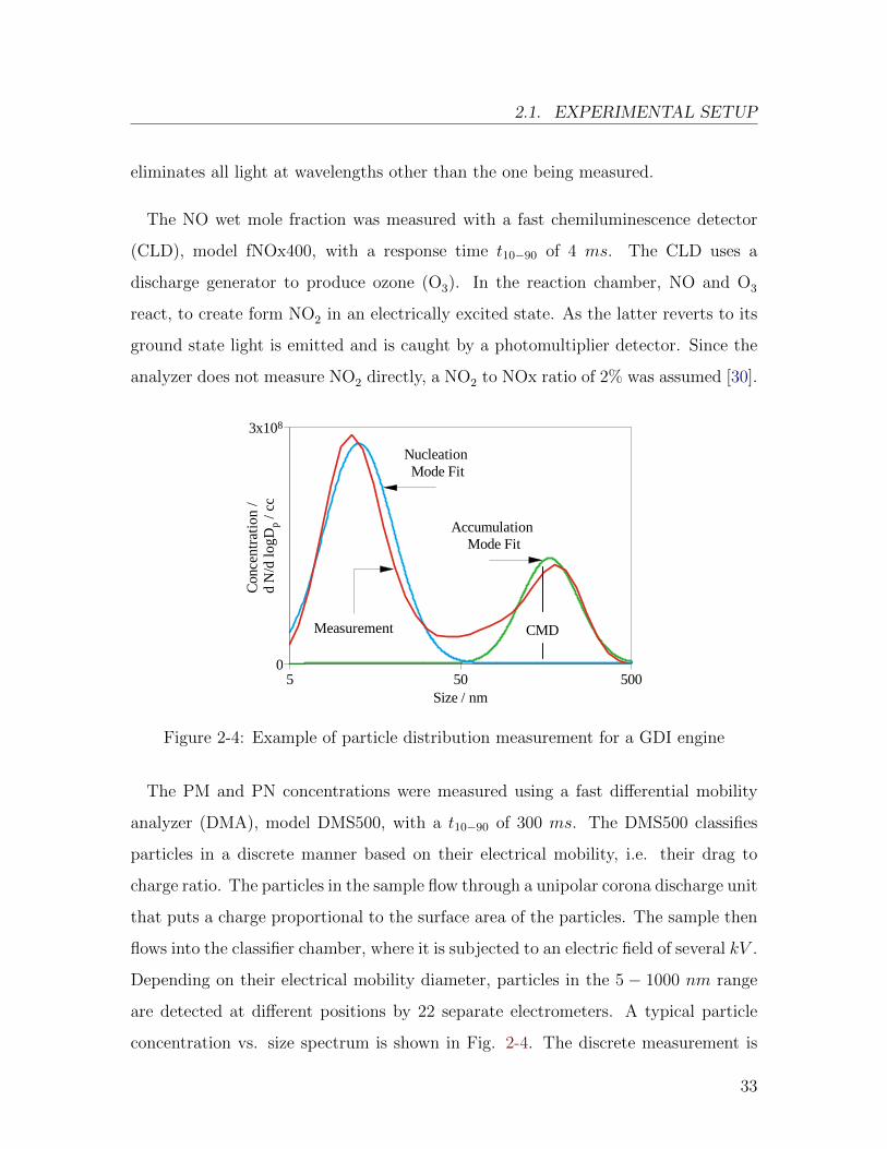
Fig. 2-4 Example of particle distribution measurement for a GDI engine . 33
Fig. 2-5 Calculated and measured λ during crank-start . . . . . . . . . . 44
Fig. 2-6 Correlation between the energy accounting methods of Section 2.4 49
9
LIST OF FIGURES
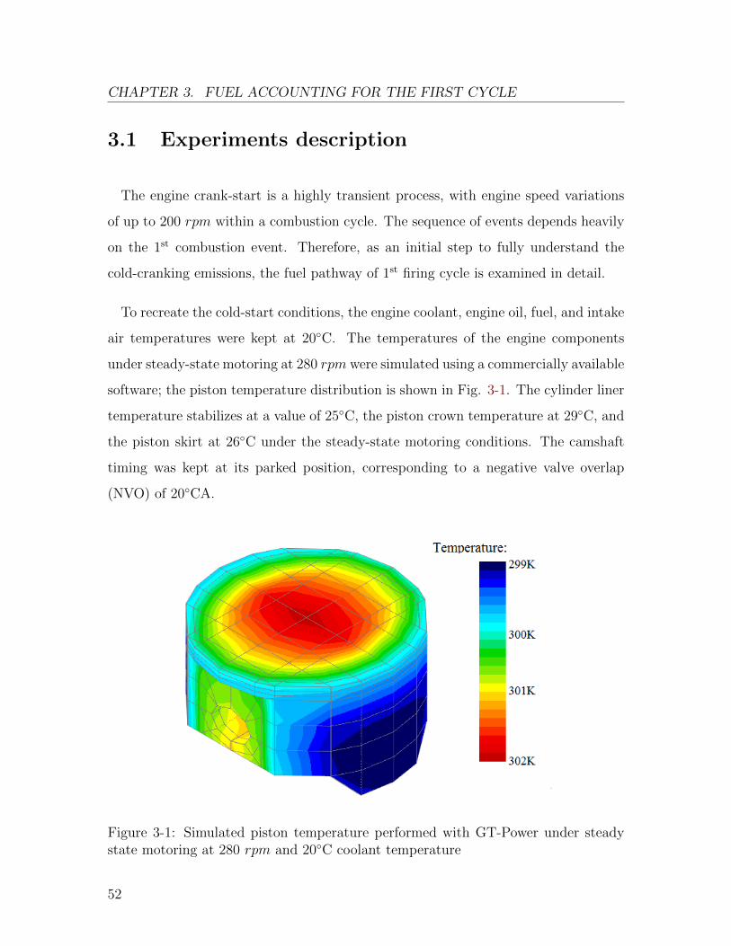
Fig. 3-1 Simulated piston temperature performed with GT-Power understeady state motoring at 280 rpm and 20◦C coolant temperature . . . 52
Fig. 3-2 Experiment description for the 1st cycle fuel accounting. (a) En-gine speed, (b) cylinder pressure, (c) intake and exhaust temperatures,and (d) normalized cumulative emissions as a function of the cyclenumber for a representative single fire experiment. . . . . . . . . . . . 53
Fig. 3-3 Exhaust mass flow of a fired cycle and a motored cycle . . . . . 56
Fig. 3-4 Fuel carbon pathway for the 1st cycle as a function of SOI . . . . 60
Fig. 3-5 Outputs of the single-cycle-fired engine as function of SOI asfollows: (a) 1st cycle NIMEP, (b) 1st cycle CO emissions, (c) 1st cyclerelative HC emissions, and (d) 2nd cycle relative HC emissions. Dashedlines correspond to a one standard deviation envelope . . . . . . . . . 61
Fig. 3-6 Fuel energy accounting for the 1st cycle as a function of SOI . . 62
Fig. 3-7 Heat release trace during the 1st cycle for different SOIs . . . . . 64
Fig. 3-8 Fuel carbon pathway for the 1st cycle as a function of FEF . . . 65
Fig. 3-9 Outputs of the single-cycle-fired engine as function of FEF asfollows: (a) 1st cycle NIMEP, (b) 1st cycle λ, (c) 1st cycle CO emissions,(d) 1st cycle relative HC emissions, (e) 2nd cycle relative HC emissions,and (f) 2nd cycle HC relative emissions as a percentage of the fuel massfor λ = 1. Dashed lines correspond to a one standard deviation envelope 66
Fig. 3-10 Fuel energy accounting for the 1st cycle as a function of FEF . . 67
Fig. 3-11 Fuel accounting for the 1st cycle vs. FEF for early compression SOI 69
Fig. 3-12 Fuel accounting for the 1st cycle vs. FEF for late compression SOI 70
Fig. 3-13 Fuel accounting for the 1st cycle vs. FEF for split injection strategy 71
Fig. 3-14 Fuel carbon pathway for the 1st cycle as a function of spark timing 72
Fig. 3-15 Outputs of the single-cycle-fired engine as function of spark timingas follows: (a) 1st cycle NIMEP, (b) 1st cycle CO emissions, (c) 1st cyclerelative HC emissions, and (d) 2nd cycle relative HC emissions. Dashedlines correspond to a one standard deviation envelope . . . . . . . . . 73
Fig. 3-16 Energy accounting for the 1st cycle as a function of spark timing 74
10
LIST OF FIGURES
Fig. 3-17 Fuel carbon pathway for the 1st cycle as a function of MAP . . . 76
Fig. 3-18 Outputs of the single-cycle-fired engine as function of MAP asfollows: (a) 1st cycle NIMEP, (b) 1st cycle gross indicated efficiency,(c) 1st cycle injected fuel mass, (d) 1st cycle HC relative emissions, and(e) 1st cycle HC absolute emissions. Dashed lines correspond to a onestandard deviation envelope . . . . . . . . . . . . . . . . . . . . . . . 77
Fig. 3-19 Fuel energy accounting for the 1st cycle as a function of MAP . . 78
Fig. 3-20 Fuel carbon pathway for the 1st cycle as a function of fuel pressure 79
Fig. 3-21 Outputs of the single-cycle-fired engine as function of fuel pressureas follows: (a) 1st cycle NIMEP, (b) 1st cycle CO emissions, (c) 1st cyclerelative HC emissions, and (d) 2nd cycle relative HC emissions. Dashedlines correspond to a one standard deviation envelope . . . . . . . . . 80
Fig. 3-22 Fuel energy accounting for the 1st cycle as a function of fuel pressure 81
Fig. 3-23 Fuel carbon pathway for the 1st cycle as a function of engine speed 82
Fig. 3-24 Outputs of the single-cycle-fired engine as function of engine speedas follows: (a) 1st cycle NIMEP, (b) 1st cycle CO emissions, (c) 1st cyclerelative HC emissions, and (d) 2nd cycle relative HC emissions. Dashedlines correspond to a one standard deviation envelope . . . . . . . . . 83
Fig. 3-25 Fuel energy accounting for the 1st cycle as a function of enginespeed . . . . . . . . . . . . . . . . . . . . . . . . . . . . . . . . . . . . 84
Fig. 4-1 Representative traces for the 1st (a), 2nd (b), and 3rd (c) cycleexperiments . . . . . . . . . . . . . . . . . . . . . . . . . . . . . . . . 89
Fig. 4-2 Continuous measurement of the particle spectrum does not achievea cycle-by-cycle resolution . . . . . . . . . . . . . . . . . . . . . . . . 90
Fig. 4-3 Exhaust gas sampling system (EGSS) for cycle-resolved particlespectrum measurement. Top: Closed position feeds ambient air to theanalyzer and circulates the exhaust gases to minimize the dead volume.Bottom: Open position feeds exhaust sample to the analyzer . . . . . 91
Fig. 4-4 1st cycle CO, NOx and HC emissions as a function of the SOI . . 93
Fig. 4-5 1st cycle PM/PN emissions and median particle size as a functionof SOI . . . . . . . . . . . . . . . . . . . . . . . . . . . . . . . . . . . 95
11
LIST OF FIGURES
Fig. 4-6 Effect of FEF on NIMEP, CO, and HC emissions for the 1st cyclefor injection strategies 1 trough 4 . . . . . . . . . . . . . . . . . . . . 96
Fig. 4-7 Effect of FEF on PM/PN emissions and median particle size forthe 1st cycle for injection strategies 1 trough 4 . . . . . . . . . . . . . 97
Fig. 4-8 Effect of FEF on NIMEP, cylinder-averaged maximum tempera-ture, and NOx emissions for the 1st cycle for injection strategies 2 and3 . . . . . . . . . . . . . . . . . . . . . . . . . . . . . . . . . . . . . . 98
Fig. 4-9 HC and PN dependence on late SOI and FEF for the 1st cycle . 100
Fig. 4-10 Effect of the FEF on the combustion phasing for 4 different injec-tion strategies . . . . . . . . . . . . . . . . . . . . . . . . . . . . . . . 101
Fig. 4-11 Effect of spark timing on 1st cycle NIMEP, CO and HC emissionsfor injection strategies 1 trough 3 . . . . . . . . . . . . . . . . . . . . 102
Fig. 4-12 Effect of spark timing on 1st cycle PM/PN emissions for injectionstrategies 1 trough 3 . . . . . . . . . . . . . . . . . . . . . . . . . . . 104
Fig. 4-13 Effect of spark timing on 1st cycle NOx emissions for injectionstrategies 2 and 3 . . . . . . . . . . . . . . . . . . . . . . . . . . . . . 105
Fig. 4-14 Simulated burned gas temperature, combustion phasing and cylin-der pressure for different ignition timings . . . . . . . . . . . . . . . . 106
Fig. 4-15 Effect of fuel pressure on 1st cycle NIMEP, CO and HC emissions 107
Fig. 4-16 Effect of fuel pressure on 1st cycle PM/PN emissions . . . . . . . 108
Fig. 4-17 Effect of fuel pressure on 1st cycle NOx emissions . . . . . . . . . 109
Fig. 4-18 2nd cycle CO, NOx, HC and PM emissions as a function of FEF 112
Fig. 4-19 2nd cycle NIMEP, CO, and HC emissions as a function of SOI . . 113
Fig. 4-20 2nd cycle PM emissions as a function of SOI . . . . . . . . . . . 114
Fig. 4-21 2nd cycle NOx emissions as a function of SOI . . . . . . . . . . . 115
Fig. 4-22 2nd cycle NIMEP, CO, and HC emissions as a function of ignitiontiming . . . . . . . . . . . . . . . . . . . . . . . . . . . . . . . . . . . 116
Fig. 4-23 2nd cycle PM emissions as a function of ignition timing . . . . . 117
12
LIST OF FIGURES
Fig. 4-24 2nd cycle NOx emissions as a function of ignition timing . . . . . 117
Fig. 4-25 Top: 2nd cycle equivalent fuel mass exhausted as a function ofthe residual fuel for FEF2nd = 1.7. Bottom: Residual fuel from the 1st
cycle as a function of FEF1st. . . . . . . . . . . . . . . . . . . . . . . 118
Fig. 4-26 Wall heat transfer as a function of FEF1st for the 1st cycle . . . . 120
Fig. 4-27 Wall heat transfer and residual fuel as a function of spark timingfor the 1st cycle . . . . . . . . . . . . . . . . . . . . . . . . . . . . . . 121
Fig. 4-28 2nd cycle equivalent fuel mass exhausted as a function of the wallheat transfer during the 1st cycle at constant residual fuel . . . . . . . 122
Fig. 4-29 2nd cycle equivalent fuel mass exhausted as a function of theresidual fuel from the 1st cycle at constant heat transfer (1st cyclemisfire) . . . . . . . . . . . . . . . . . . . . . . . . . . . . . . . . . . . 123
Fig. 4-30 3rd cycle CO, NOx, HC and PM emissions as a function of FEF 125
Fig. 4-31 3rd cycle NIMEP, CO, and HC emissions as a function of SOI . . 126
Fig. 4-32 3rd cycle PM and NOx emissions as a function of SOI . . . . . . 128
Fig. 4-33 3rd cycle NIMEP, CO, and HC emissions as a function of sparktiming . . . . . . . . . . . . . . . . . . . . . . . . . . . . . . . . . . . 128
Fig. 4-34 3rd cycle PM and NOx emissions as a function of spark timing . 129
Fig. 5-1 Baseline intake and exhaust timings and direction of phasing forthe other investigated valve timings . . . . . . . . . . . . . . . . . . . 134
Fig. 5-2 Combustion lambda and CA50 during the crank-start process forall four valve timings studied . . . . . . . . . . . . . . . . . . . . . . . 136
Fig. 5-3 Air velocity at intake valve as a function of IVO timing; simulationresults . . . . . . . . . . . . . . . . . . . . . . . . . . . . . . . . . . . 136
Fig. 5-4 Left: Simulated in-cylinder pressure during intake stroke for thefirst engine cycle and different IVO timings. Right: Saturated vaporpressure at 25◦C of the main constituents of the certification gasolineUTG-91 . . . . . . . . . . . . . . . . . . . . . . . . . . . . . . . . . . 137
Fig. 5-5 Simplified thermodynamic analysis of the filling process . . . . . 138
13
LIST OF FIGURES
Fig. 5-6 Final temperature after cylinder filling as a function of pressureat IVO for the simplified system . . . . . . . . . . . . . . . . . . . . . 139
Fig. 5-7 Simulated in-cylinder temperature during the intake stroke forthe first engine cycle and different IVO timings . . . . . . . . . . . . 140
Fig. 5-8 Effective compression ratio for the 1st cycle as a function of IVO 141
Fig. 5-9 Valve timing diagram for the late IVO/IVC setting . . . . . . . . 141
Fig. 5-10 CO production (top) and 1st cycle fuel requirement (bottom) asa function of combustion λ for baseline and late IVO settings . . . . . 142
Fig. 5-11 1st cycle HC emissions and particle median size as a function ofSOI for both baseline and late IVO cases . . . . . . . . . . . . . . . . 143
Fig. 5-12 Mixture formation process during the 2nd cycle . . . . . . . . . . 144
Fig. 5-13 NIMEP, engine speed and MAP traces during cold crank-start forbaseline and late IVO. Symbols are for individual run results; coloredlines represent average values of 5 separate runs . . . . . . . . . . . . 145
Fig. 5-14 Cycle-by-cycle and cumulative NOx, HC, and PM emissions ofcylinder 4 during cold crank-start for the baseline and late IVO settings146
Fig. 5-15 Simulated residual gas fraction and in-cylinder temperature dur-ing the intake stroke for the 2nd engine cycle and different EVC timings148
Fig. 5-16 Valve timing diagram for the early EVO/EVC setting . . . . . . 148
Fig. 5-17 Baseline and early EVC results for the lambda of combustion asa function of the injected fuel amount for the 1st and 2nd engine cycles 149
Fig. 5-18 NIMEP, engine speed and MAP traces during cold crank-start forbaseline and early EVC. Symbols are for individual run results; coloredlines represent mean values of 5 separate runs . . . . . . . . . . . . . 150
Fig. 5-19 Work output losses caused by early EVO/EVC . . . . . . . . . . 151
Fig. 5-20 Cycle-by-cycle and cumulative NOx, HC, and PM emissions ofcylinder 4 during cold crank-start for the baseline and early EVC settings152
Fig. 5-21 Valve timing diagram for the early EVO/EVC setting . . . . . . 153
14
LIST OF FIGURES
Fig. 5-22 NIMEP, engine speed and MAP traces during cold crank-start forbaseline and symmetric NVO. Symbols are for individual run results;colored lines represent mean values of 5 separate runs . . . . . . . . . 154
Fig. 5-23 Cycle-by-cycle and cumulative NOx, HC, and PM emissions ofcylinder 4 during cold crank-start for the baseline and symmetric NVOsettings . . . . . . . . . . . . . . . . . . . . . . . . . . . . . . . . . . 155
Fig. 6-1 Diagram of the experimental setup and the sensor locations . . . 160
Fig. 6-2 Concentration and mass flow of NOx, HC and PM as a functionof lambda . . . . . . . . . . . . . . . . . . . . . . . . . . . . . . . . . 162
Fig. 6-3 Particle size distribution of the accumulation mode (lognormalfit) as a function of lambda (λ = 0.95− 1.05 and a 0.025 step) . . . . 163
Fig. 6-4 Combustion phasing, CoV of NIMEP and exhaust mass flow as afunction of lambda . . . . . . . . . . . . . . . . . . . . . . . . . . . . 164
Fig. 6-5 Split injection strategy A: Combustion stability and mass flowemissions of NOx, HC and PM as a function of split ratio . . . . . . . 165
Fig. 6-6 Split injection strategy A: Particle size distribution of the mea-sured spectrum as a function of split ratio . . . . . . . . . . . . . . . 166
Fig. 6-7 Split injection strategy B: Combustion stability and mass flowemissions of NOx, HC and PM as a function of split ratio . . . . . . . 167
Fig. 6-8 Split injection strategy B: Particle size distribution of the mea-sured spectrum as a function of split ratio . . . . . . . . . . . . . . . 168
Fig. 6-9 Split injection strategy C: Combustion stability and mass flowemissions of NOx, HC and PM as a function of late injection pulseduration . . . . . . . . . . . . . . . . . . . . . . . . . . . . . . . . . . 169
Fig. 6-10 Split injection strategy C: Particle size distribution of the ac-cumulation mode (lognormal fit) as a function of late injection pulseduration . . . . . . . . . . . . . . . . . . . . . . . . . . . . . . . . . . 170
Fig. 6-11 Emissions indices and indicated specific emissions of NOx, HCand PM as a function of CA50 for three different injection strategies . 172
Fig. 6-12 Experimental P-V diagram and cylinder temperature for threedifferent combustion phasing using the Double injection strategy . . 173
15
LIST OF FIGURES
Fig. 6-13 Simulated NOx emissions as a function of CA50 . . . . . . . . . 174
Fig. 6-14 Combustion stability and exhaust thermal enthalpy as a functionof CA50 for three different injection strategies . . . . . . . . . . . . . 177
Fig. 6-15 Baseline intake and exhaust timings and direction of phasing forthe other investigated valve timings . . . . . . . . . . . . . . . . . . . 178
Fig. 6-16 Residual gas fraction at cold fast-idle as a function of valve timing 179
Fig. 6-17 Simulated engine-out NOx mole fraction during cold fast-idle forEGR rates and combustion phasing at stoichiometric combustion andfixed valve timing . . . . . . . . . . . . . . . . . . . . . . . . . . . . . 180
Fig. 6-18 Emissions indices and indicated specific emissions of NOx, HCand PM as a function of CA50 for baseline and two early EVC settings 182
Fig. 6-19 Combustion stability and exhaust thermal enthalpy as a functionof CA50 for baseline and two early EVC settings . . . . . . . . . . . . 183
Fig. 6-20 Simulated engine-out NOx emissions during cold fast-idle for dif-ferent operation strategies at stoichiometric combustion . . . . . . . . 185
Fig. 6-21 Effective compression ratio and modeled cylinder peak tempera-ture as a function of intake valve timing delay during cold fast-idle . . 185
Fig. 6-22 Crank angle resolved port-measurements of the HC emissionsat cold fast-idle conditions for 3 different valve timings at CA50 =40◦CA aTDCcomp.. Color lines represent the average over 150 cycles . 187
Fig. 6-23 Emissions indices and indicated specific emissions of NOx, HCand PM as a function of CA50 for baseline and two symmetric NVOsettings . . . . . . . . . . . . . . . . . . . . . . . . . . . . . . . . . . 188
Fig. 6-24 Accumulation mode particle spectrum at cold fast-idle conditionsfor each valve timing CA50 = 40◦CA aTDCcomp.. Measurements werefitted to a lognormal distribution. Color lines represent the averageover 150 cycles . . . . . . . . . . . . . . . . . . . . . . . . . . . . . . 189
Fig. 6-25 Combustion stability and exhaust thermal enthalpy as a functionof CA50 for baseline and two symmetric NVO settings . . . . . . . . 190
16
LIST OF TABLES
List of Tables
Table 2.1 Specifications of the GM - LNF engine . . . . . . . . . . . . . . 30
Table 2.2 Stock parked valve timing. Valve events reported at 0.2 mm lift 30
Table 3.1 Experimental scope for the 1st cycle fuel accounting analysis . . 54
Table 3.2 Extended injection strategy study of the 1st cycle’s FEF . . . . 69
Table 4.1 1st cycle strategy for 2nd cycle experiments . . . . . . . . . . . 90
Table 4.2 Experimental scope for the 1st cycle emissions . . . . . . . . . . 92
Table 4.3 Experimental scope for the 2nd cycle emissions . . . . . . . . . 111
Table 4.4 1st cycle strategy for 2nd cycle experiments . . . . . . . . . . . 111
Table 4.5 Experimental scope for the 3rd cycle emissions . . . . . . . . . 124
Table 4.6 1st and 2nd cycle strategies for 3rd cycle experiments . . . . . . 125
Table 4.7 Effect of spray/valve interaction on NIMEP and HC emissions. 127
Table 5.1 Valve setting cases for the crank-start study . . . . . . . . . . . 135
Table 6.1 Experimental conditions for cold fast-idle experiments . . . . . 159
Table 6.2 Injection strategy for lambda sweep . . . . . . . . . . . . . . . 161
Table 6.3 Split injection strategy A . . . . . . . . . . . . . . . . . . . . . 164
Table 6.4 Split injection strategy B . . . . . . . . . . . . . . . . . . . . . 164
Table 6.5 Split injection strategy C . . . . . . . . . . . . . . . . . . . . . 165
Table 6.6 Strategies used for the combustion phasing study at cold fast-idle 171
17

LIST OF TABLES
Table 6.7 Valve setting cases for the cold fast-idle study . . . . . . . . . . 179
18
Chapter 1
Introduction
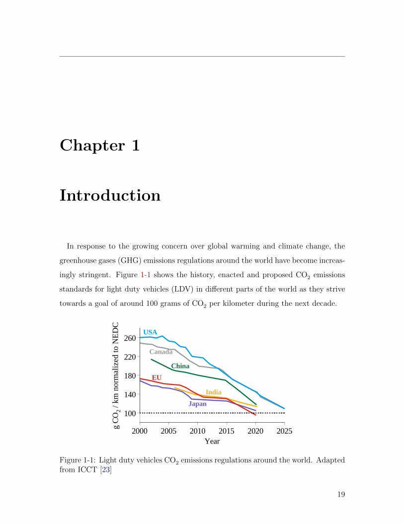
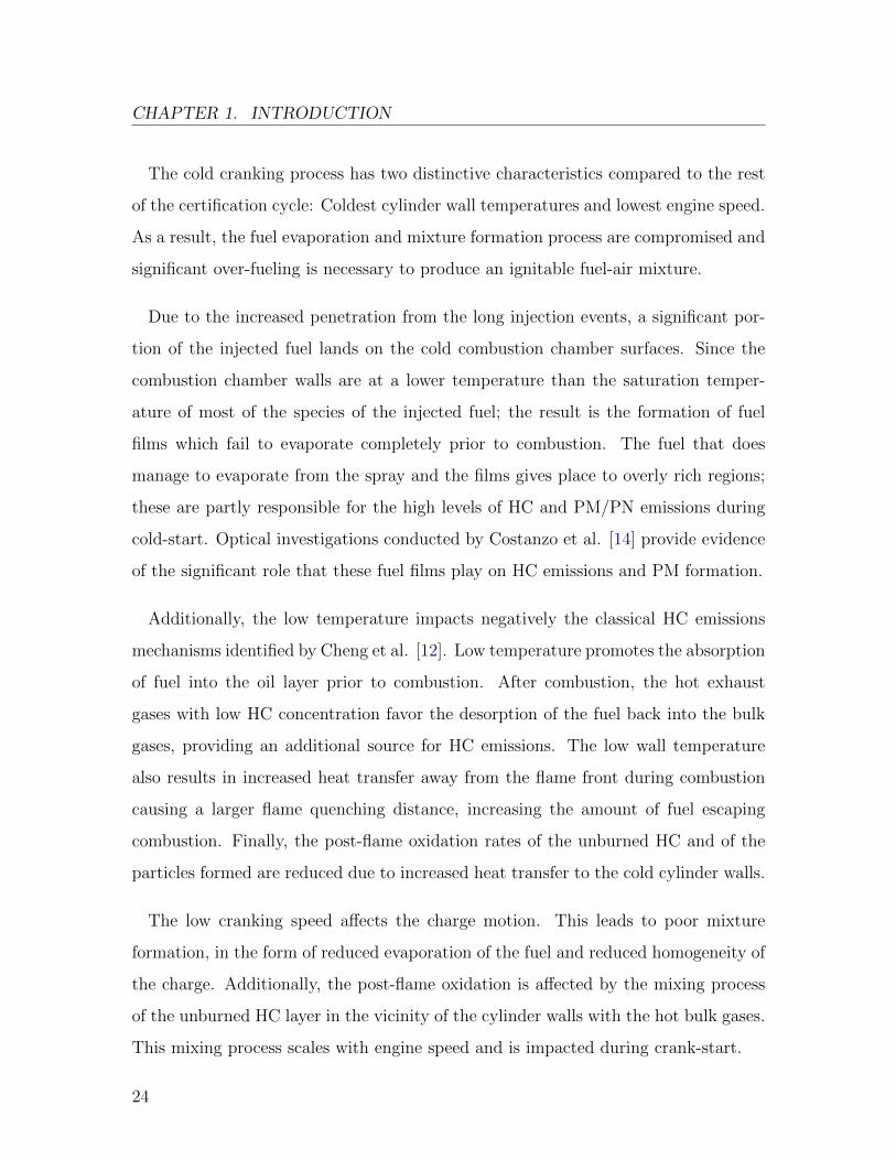
In response to the growing concern over global warming and climate change, the
greenhouse gases (GHG) emissions regulations around the world have become increas-
ingly stringent. Figure 1-1 shows the history, enacted and proposed CO2 emissions
standards for light duty vehicles (LDV) in different parts of the world as they strive
towards a goal of around 100 grams of CO2 per kilometer during the next decade.
Canada
China
India
Japan
EU
g C
O2
/ km
nor
mal
ized
to N
ED
C
100
140
180
220
260
Year2000 2005 2010 2015 2020 2025
USA
Figure 1-1: Light duty vehicles CO2 emissions regulations around the world. Adaptedfrom ICCT [23]
19
CHAPTER 1. INTRODUCTION
Friction
Reduction
3.5 – 4.8%
VVT
4.1 – 5.5%
Advanced
GDI
17 – 25%
CO2
reduction
potential
High Eff.
Gearbox
2– 13%
Advanced
Diesel
19 – 22%
EV
100%PHEV
63 %
Mild Hybrid
7.2 %
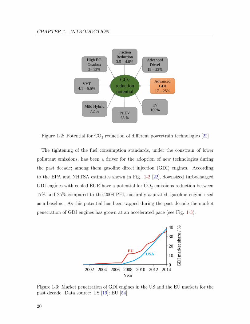
Figure 1-2: Potential for CO2 reduction of different powertrain technologies [22]
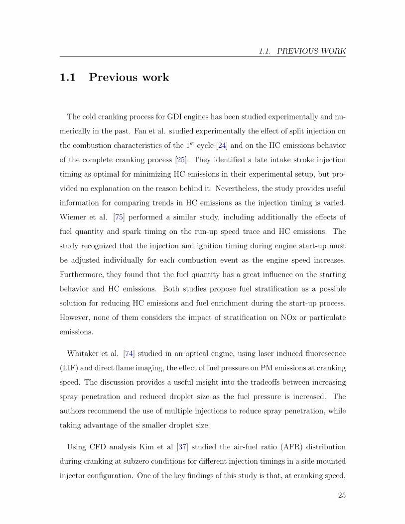
The tightening of the fuel consumption standards, under the constrain of lower
pollutant emissions, has been a driver for the adoption of new technologies during
the past decade; among them gasoline direct injection (GDI) engines. According
to the EPA and NHTSA estimates shown in Fig. 1-2 [22], downsized turbocharged
GDI engines with cooled EGR have a potential for CO2 emissions reduction between
17% and 25% compared to the 2008 PFI, naturally aspirated, gasoline engine used
as a baseline. As this potential has been tapped during the past decade the market
penetration of GDI engines has grown at an accelerated pace (see Fig. 1-3).
GD
I mar
ket s
hare
/ %
0
10
20
30
40
Year2002 2004 2006 2008 2010 2012 2014
EUUSA
Figure 1-3: Market penetration of GDI engines in the US and the EU markets for thepast decade. Data source: US [19]; EU [54]
20
GDI engines have better knock resistance through charge cooling, allow for aggres-
sive scavenging to improve the low-end torque of turbo-charged engines – without the
risk of short-circuiting fresh unburned mixture – and have extended lean operation
limits with the associated reduction in pumping losses. On the other hand, the direct
liquid injection poses some emissions challenges, especially for HC and PM during
the cold-start phase.
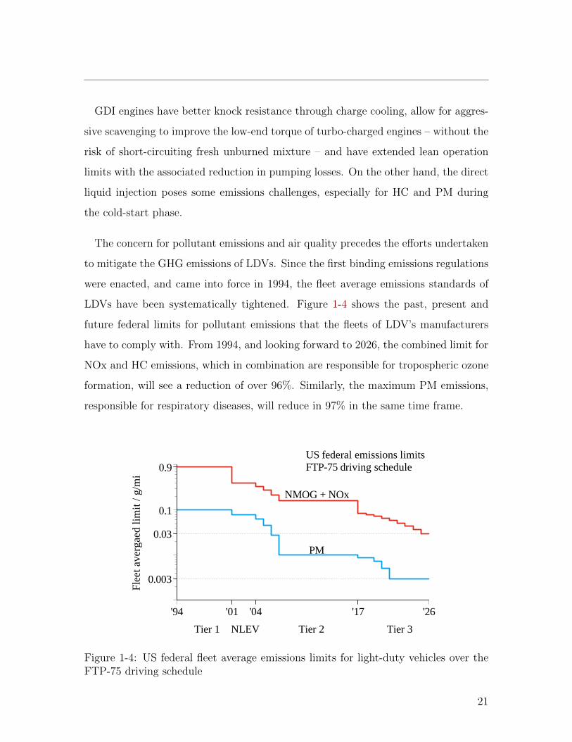
The concern for pollutant emissions and air quality precedes the efforts undertaken
to mitigate the GHG emissions of LDVs. Since the first binding emissions regulations
were enacted, and came into force in 1994, the fleet average emissions standards of
LDVs have been systematically tightened. Figure 1-4 shows the past, present and
future federal limits for pollutant emissions that the fleets of LDV’s manufacturers
have to comply with. From 1994, and looking forward to 2026, the combined limit for
NOx and HC emissions, which in combination are responsible for tropospheric ozone
formation, will see a reduction of over 96%. Similarly, the maximum PM emissions,
responsible for respiratory diseases, will reduce in 97% in the same time frame.
Tier 1 Tier 2 Tier 3NLEV
Fle
et a
verg
aed
limit
/ g/m
i
0.003
0.03
0.9
0.1
'01 '04 '17'94 '26
NMOG + NOx
PM
US federal emissions limitsFTP-75 driving schedule
Figure 1-4: US federal fleet average emissions limits for light-duty vehicles over theFTP-75 driving schedule
21
CHAPTER 1. INTRODUCTION
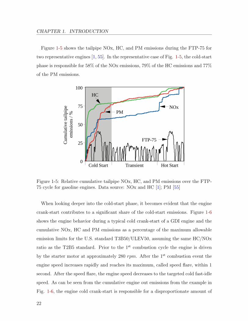
Figure 1-5 shows the tailpipe NOx, HC, and PM emissions during the FTP-75 for
two representative engines [1, 55]. In the representative case of Fig. 1-5, the cold-start
phase is responsible for 58% of the NOx emissions, 79% of the HC emissions and 77%
of the PM emissions.
Cold Start Hot StartTransient
NOx
Cum
ulat
ive
tail
pipe
em
issi
ons
/ %
0
25
50
75
100
HC
FTP-75
PM
Figure 1-5: Relative cumulative tailpipe NOx, HC, and PM emissions over the FTP-75 cycle for gasoline engines. Data source: NOx and HC [1]; PM [55]
When looking deeper into the cold-start phase, it becomes evident that the engine
crank-start contributes to a significant share of the cold-start emissions. Figure 1-6
shows the engine behavior during a typical cold crank-start of a GDI engine and the
cumulative NOx, HC and PM emissions as a percentage of the maximum allowable
emission limits for the U.S. standard T3B50/ULEV50, assuming the same HC/NOx
ratio as the T2B5 standard. Prior to the 1st combustion cycle the engine is driven
by the starter motor at approximately 280 rpm. After the 1st combustion event the
engine speed increases rapidly and reaches its maximum, called speed flare, within 1
second. After the speed flare, the engine speed decreases to the targeted cold fast-idle
speed. As can be seen from the cumulative engine out emissions from the example in
Fig. 1-6, the engine cold crank-start is responsible for a disproportionate amount of
22
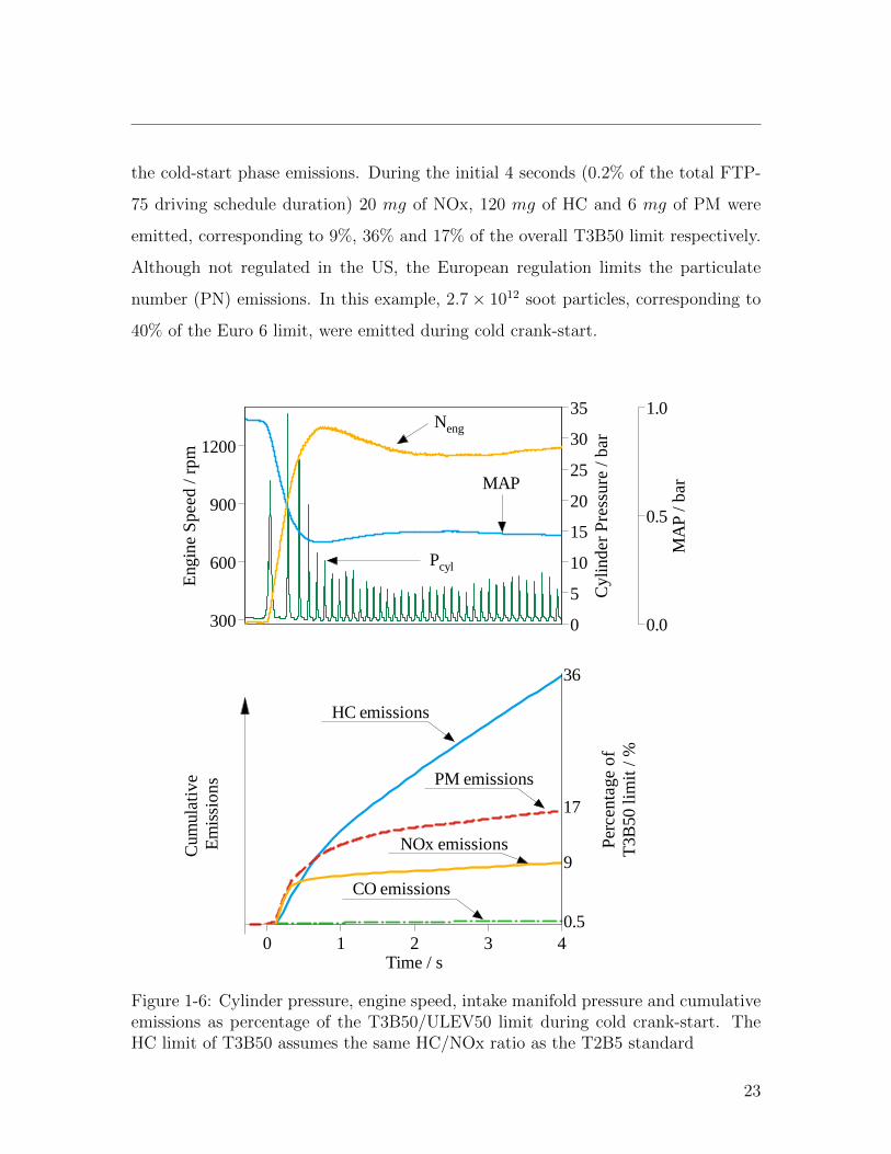
the cold-start phase emissions. During the initial 4 seconds (0.2% of the total FTP-
75 driving schedule duration) 20 mg of NOx, 120 mg of HC and 6 mg of PM were
emitted, corresponding to 9%, 36% and 17% of the overall T3B50 limit respectively.
Although not regulated in the US, the European regulation limits the particulate
number (PN) emissions. In this example, 2.7× 10¹² soot particles, corresponding to
40% of the Euro 6 limit, were emitted during cold crank-start.
Perc
enta
ge o
fT
3B50
lim
it /
%
0.5
9
17
36
HC emissions
Cum
ulat
ive
Em
issi
ons
CO emissions
PM emissions
NOx emissions
Time / s0 1 2 3 4
Cyl
inde
r P
ress
ure
/ bar
0
5
10
15
20
25
30
35
MA
P / b
ar
0.0
0.5
1.0
Eng
ine
Spe
ed /
rpm
300
600
900
1200
Neng
MAP
Pcyl
Figure 1-6: Cylinder pressure, engine speed, intake manifold pressure and cumulativeemissions as percentage of the T3B50/ULEV50 limit during cold crank-start. TheHC limit of T3B50 assumes the same HC/NOx ratio as the T2B5 standard
23
CHAPTER 1. INTRODUCTION
The cold cranking process has two distinctive characteristics compared to the rest
of the certification cycle: Coldest cylinder wall temperatures and lowest engine speed.
As a result, the fuel evaporation and mixture formation process are compromised and
significant over-fueling is necessary to produce an ignitable fuel-air mixture.
Due to the increased penetration from the long injection events, a significant por-
tion of the injected fuel lands on the cold combustion chamber surfaces. Since the
combustion chamber walls are at a lower temperature than the saturation temper-
ature of most of the species of the injected fuel; the result is the formation of fuel
films which fail to evaporate completely prior to combustion. The fuel that does
manage to evaporate from the spray and the films gives place to overly rich regions;
these are partly responsible for the high levels of HC and PM/PN emissions during
cold-start. Optical investigations conducted by Costanzo et al. [14] provide evidence
of the significant role that these fuel films play on HC emissions and PM formation.
Additionally, the low temperature impacts negatively the classical HC emissions
mechanisms identified by Cheng et al. [12]. Low temperature promotes the absorption
of fuel into the oil layer prior to combustion. After combustion, the hot exhaust
gases with low HC concentration favor the desorption of the fuel back into the bulk
gases, providing an additional source for HC emissions. The low wall temperature
also results in increased heat transfer away from the flame front during combustion
causing a larger flame quenching distance, increasing the amount of fuel escaping
combustion. Finally, the post-flame oxidation rates of the unburned HC and of the
particles formed are reduced due to increased heat transfer to the cold cylinder walls.
The low cranking speed affects the charge motion. This leads to poor mixture
formation, in the form of reduced evaporation of the fuel and reduced homogeneity of
the charge. Additionally, the post-flame oxidation is affected by the mixing process
of the unburned HC layer in the vicinity of the cylinder walls with the hot bulk gases.
This mixing process scales with engine speed and is impacted during crank-start.
24
1.1. PREVIOUS WORK
1.1 Previous work
The cold cranking process for GDI engines has been studied experimentally and nu-
merically in the past. Fan et al. studied experimentally the effect of split injection on
the combustion characteristics of the 1st cycle [24] and on the HC emissions behavior
of the complete cranking process [25]. They identified a late intake stroke injection
timing as optimal for minimizing HC emissions in their experimental setup, but pro-
vided no explanation on the reason behind it. Nevertheless, the study provides useful
information for comparing trends in HC emissions as the injection timing is varied.
Wiemer et al. [75] performed a similar study, including additionally the effects of
fuel quantity and spark timing on the run-up speed trace and HC emissions. The
study recognized that the injection and ignition timing during engine start-up must
be adjusted individually for each combustion event as the engine speed increases.
Furthermore, they found that the fuel quantity has a great influence on the starting
behavior and HC emissions. Both studies propose fuel stratification as a possible
solution for reducing HC emissions and fuel enrichment during the start-up process.
However, none of them considers the impact of stratification on NOx or particulate
emissions.
Whitaker et al. [74] studied in an optical engine, using laser induced fluorescence
(LIF) and direct flame imaging, the effect of fuel pressure on PM emissions at cranking
speed. The discussion provides a useful insight into the tradeoffs between increasing
spray penetration and reduced droplet size as the fuel pressure is increased. The
authors recommend the use of multiple injections to reduce spray penetration, while
taking advantage of the smaller droplet size.
Using CFD analysis Kim et al [37] studied the air-fuel ratio (AFR) distribution
during cranking at subzero conditions for different injection timings in a side mounted
injector configuration. One of the key findings of this study is that, at cranking speed,
25
CHAPTER 1. INTRODUCTION
increased charge motion affects negatively the low AFR necessary around the spark
plug for successful combustion. Since the direction of the tumble motion induced
by the injection spray is opposite to the intake tumble, different combinations of
intake valve opening and injection timing will result in different AFR around the
spark plug, thus providing some light to explain the observations of the experimental
studies presented above.
Similarly, Malaguti et al. performed numerical analysis for the initial combustion
cycles, focusing on spray-wall interaction and its effect in fuel evaporation and liquid
fuel film formation [52, 53]. They found that interaction between the intake valve and
the injection spray results in the formation of fuel films in the cylinder head in the
vicinity of the spark plug. Additionally, they found that fuel films on the combustion
chamber walls are the main sources for fuel evaporation, and that the contribution
from the flying fuel droplets evaporation is only relevant during the early compression
stroke.
Xu et al. [78] went further in the CFD modeling of the cranking process, including
engine run-up for different split injection strategies. The numerical results show
that the optimum split injection strategy depends strongly on the engine speed, and
therefore the injection strategy must be actively adjusted during the run-up process.
In the same way as Malaguti et al. [52, 53], Xu et al. identified the importance of
the rich cloud around the spark plug, and the ability of the fuel spray momentum to
create flow structures that enable low AFR at the ignition point.
This paper also builds upon the methodology developed at the Sloan Automotive
Laboratory at MIT for experimentally studying the 1st combustion cycle and the
cranking process in port-fuel injected spark ignition engines. This previous work
includes the use of fast FID and fast NDIR for HC, CO and CO2 measurement, and
of a fast response sampling system for the cycle resolved measurement of the exhaust
composition [10, 11, 38, 45, 46, 65].
26
1.2. PROJECT FOCUS
1.2 Project focus
This project is part of a wider effort undertaken at the Sloan Automotive Lab-
oratory at the Massachusetts Institute of Technology to understand and mitigate
the emissions challenges of gasoline direct injection engines, specifically during the
cold-start phase [9, 15, 48, 57, 58, 72].
The goal of the present study is to gain a deeper understanding of the processes
leading the formation of pollutants during the cold-start phase of a wall guided gaso-
line direct injection engine. To accomplish this, the engine-out NOx, HC and PM
emissions are studied in detail for a variety of operation strategies during the cold
crank-start and the cold fast-idle periods.
For the crank-start process, a special emphasis was placed on understanding the
sensitivity of the mixture formation process, of the fuel pathway and of the NOx,
HC, and PM emissions to the operation strategy of the individual combustion events
during cranking. The effects of the heat transfer history and the residual fuel from
previous injection events on the mixture formation process are also considered.
The investigations of the fast-idle period are focused on understanding and quan-
tifying the different tradeoffs present between the engine-out emissions of pollutants,
NOx, HC and PM, the combustion stability and the exhaust thermal enthalpy flow
to the catalyst for several operation strategies.
An opportunity investigated in this work is the potential of unconventional valve
timing, resulting in large negative valve overlap (NVO), for reducing the engine-
out emissions during the cold crank-start and fast-idle phases of a GDI engine. As
the authority of variable valve timing systems increases, new parked (de-energized)
camshaft positions become possible. The merit of these parked positions for cold-start
emissions control is studied in detail.
27

– Intentionally left blank –
Chapter 2
Methodology
This chapter provides a detailed description of the experimental and numerical
methodology followed to quantify the engine-out emissions during the cold-start pro-
cess and the energy release analysis during combustion. A special emphasis is placed
on the challenges and solutions implemented for dealing with the highly transient
processes taking place during engine crank-start.
2.1 Experimental setup
2.1.1 Engine base
The experiments were carried out using a commercial 4-cylinder GDI turbo-charged
engine with a displacement volume of 499.5 cm3 per cylinder, a square stroke ratio and
a compression ratio of 9.2. The engine used side-mounted electromagnetic injectors,
with a 52◦ cone angle, a 25◦ inclination from the horizontal and 6 holes. The engine
also featured a centrally mounted spark plug and 4 valves per cylinder. The valve
29
CHAPTER 2. METHODOLOGY
timing corresponding to the stock parked position of the camshafts resulted in a
negative valve overlap of 20◦CA. The engine had variable valve timing (VVT) on both
the intake and exhaust camshafts. The VVT system was hydraulically actuated, had
an authority of 50◦CA on each camshaft and allowed the advancing of the intake and
the retarding of the exhaust timing. Further details are shown in Tables 2.1 and 2.2.
Engine type In-line 4 cylinderDisplacement 1998 ccBore / Stroke 86/86 mmConnecting rod 145.5 mmCompression ratio 9.2 : 1
Injector type Side mounted, 6-hole, electromagneticSpray cone angle 52◦
Injector inclination 25◦
Table 2.1: Specifications of the GM - LNF engine
Intake Valve Opening (IVO) 11◦CA aTDCIntake Valve Closing (IVC) 61◦CA aBDCMax. intake valve lift 10.3 mm @ 126◦CA aTDC
Exhaust Valve Opening (EVO) 52◦CA bBDCExhaust Valve Closing (EVC) 10◦CA bTDCMax. exhaust valve lift 10.3 mm @ 125◦CA aTDC
Table 2.2: Stock parked valve timing. Valve events reported at 0.2 mm lift
The engine control is achieved by an in-house developed injection control software,
allowing a full customization of the engine parameters such as injection and spark
timings, injection duration, injection split ratio and intake/exhaust cam phasing. In
actual GDI applications, typical fuel pressures for the initial injection events during
crank-start ranges between 30 and 70 bar [4, 71] and is heavily dependent on engine
speed. In the experimental setup used in this study, the fuel pressure was kept
independent from engine operation and was maintained at a constant value by a
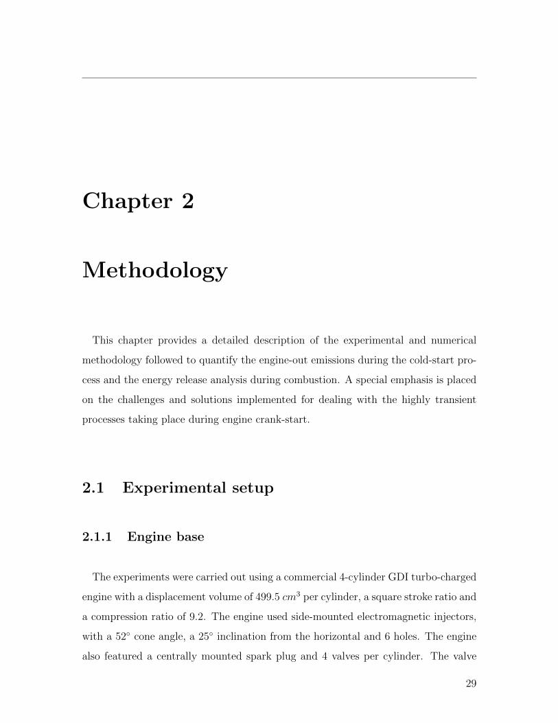
hydro-pneumatic accumulator. Figure 2-1 shows further detail of the setup.
30
2.1. EXPERIMENTAL SETUP
4
3
2
1
N2
FuelCoolant
λ
m
PT
T
T
T
P
TP
T
TP
T
Figure 2-1: Diagram of the experimental setup and the sensor locations
The engine used a Tier II EEE certification gasoline produced by Haltermann So-
lutions (HF0437) with a carbon mass fraction of 86.5%, and 29% aromatics content.
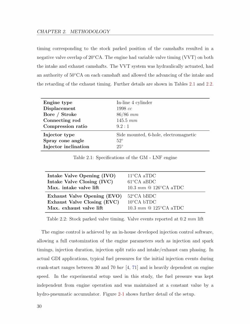
The fuel’s RON and MON were 96.6 and 88.5 respectively. The Reid vapor pressure
was 62.7 kPa with the distillation curve is shown in Fig. 2-2. The cold-start condi-
tions were maintained as close to 20◦C as possible by three independent chillers for
the fuel, intake air, and engine oil and coolant.
Tem
pera
ture
/ °C
30
60
90
120
150
180
210
Evaporated fraction / %0 20 40 60 80 100
Figure 2-2: Distillation curve of the Tier II EEE certification gasoline used
31
CHAPTER 2. METHODOLOGY
2.1.2 Emissions measurement
The exhaust composition was measured using fast response analyzers from Cambus-
tion. The wet HC mole fraction was measured using a fast flame ionization detector
(FFID), model HFR400, with a response time t10−90 of 1 ms. The working principle
of the FFID is based on the ionization of HC molecules under a hydrogen-air diffusion
flame [13]. The carbon ion flow generated is attracted to the collector plate and an
electrometer is used to measure the current, which is proportional to the number of
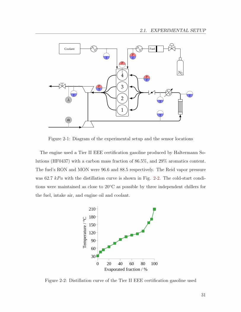
carbon atoms present in the sample. Varying O2 concentration in the sample cre-
ates difficulties for interpreting the output signal due to the competition between ion
formation in the flame and their consumption by oxygen. To correct the measure-
ments at lean operation, the change in sensitivity at different O2 mole fractions was
measured and it is shown in Fig. 2-3; the change in sensitivity is less than 5%.
Rel
ativ
e ch
ange
in s
igna
l / -
0.94
0.96
0.98
1.00
O2 mole fraction in sample / %
0 5 10 15 20
Figure 2-3: Effect of O2 on FID. Measurement of 4500 ppm of C3H8; balance N2
The CO and CO2 wet mole fractions were measured with a fast non-dispersive
infrared (NDIR) analyzer, model NDIR500, with a response time t10−90 of 8 ms. In
NDIR sensors, a radiating IR source, usually an incandescent filament, is employed
to emit a wide IR spectrum through the sensor’s sample body. The amount of IR
light absorbed at a certain wavelength is proportional to the concentration of the
corresponding component. The light detector has a rotating filter in front of it that
32
2.1. EXPERIMENTAL SETUP
eliminates all light at wavelengths other than the one being measured.
The NO wet mole fraction was measured with a fast chemiluminescence detector
(CLD), model fNOx400, with a response time t10−90 of 4 ms. The CLD uses a
discharge generator to produce ozone (O3). In the reaction chamber, NO and O3
react, to create form NO2 in an electrically excited state. As the latter reverts to its
ground state light is emitted and is caught by a photomultiplier detector. Since the
analyzer does not measure NO2 directly, a NO2 to NOx ratio of 2% was assumed [30].
Con
cent
rati
on /
d N
/d lo
gDp
/ cc
0
3x10⁸
Size / nm5 50 500
Measurement
Nucleation Mode Fit
Accumulation Mode Fit
CMD
Figure 2-4: Example of particle distribution measurement for a GDI engine
The PM and PN concentrations were measured using a fast differential mobility
analyzer (DMA), model DMS500, with a t10−90 of 300 ms. The DMS500 classifies
particles in a discrete manner based on their electrical mobility, i.e. their drag to
charge ratio. The particles in the sample flow through a unipolar corona discharge unit
that puts a charge proportional to the surface area of the particles. The sample then
flows into the classifier chamber, where it is subjected to an electric field of several kV .
Depending on their electrical mobility diameter, particles in the 5 − 1000 nm range
are detected at different positions by 22 separate electrometers. A typical particle
concentration vs. size spectrum is shown in Fig. 2-4. The discrete measurement is
33
CHAPTER 2. METHODOLOGY
fitted by two lognormal distributions, corresponding to the nucleation mode and to
the accumulation mode. Since the European Particle Measurement Program (PMP)
requires the removal of the volatile fraction, and given the low contribution of volatile
particles to PM, the metric of interest is the accumulation mode. In addition the
sampling temperature was kept at 150◦C to prevent volatiles from condensing on the
accumulation mode particles.
The number of particles per standard cubic centimeter (#/scc) can be found by
integrating the lognormal distribution for the accumulation mode. The volume con-
centration of the number of particles, N is:
N[ #
scc
]=
∫ 1000 nm
5 nm
d N
d log(Dp)d log(Dp) (2.1)
Where Dp is the particle size and dN/dlog(Dp) is the particle concentration number
for a the size range represented by Dp. The calculation of the mass concentration from
the size spectrum measurement requires additional consideration of the morphology
of the soot particles and of their specific gravity. The volume is proportional to Dkp ,
where k = 3 is the recommended fractal dimension for GDI engines. In other words,
spherical particles are assumed with a specific gravity of 1. The volume concentration
of the particle mass, M is:
M[ µgscc
]=
∫ 1000 nm
5 nm
d N
d log(Dp)· (5.20× 10⁻¹⁶ ·Dp3) · d log(Dp) (2.2)
2.1.3 Measurement of cylinder pressure
The in-cylinder pressure is measured with a high-temperature piezoelectric pres-
sure transducer, Kistler 6125A, mounted in the cylinder head between the intake and
34
2.1. EXPERIMENTAL SETUP
exhaust valves and approximately 2 cm from the cylinder wall. The charge output of
the pressure sensors was amplified and converted to an analog signal using a charge
amplifier, Kistler 5010b. Due to the operation principle of the metaloxidesemicon-
ductor field-effect transistor (MOSFET) used for the charge amplifying, the signal
exhibits a long-term drift at an approximate rate of 0.03 pC/s [43].
At steady-state operation the cylinder pressure can be corrected by referencing, or
pegging, the pressure sensor output to a known absolute pressure level. The intake
manifold absolute pressure sensor was used for this end. The pegging of the signals
was done at the beginning of the compression stroke, where, due to the low piston
and flow speeds, the intake manifold and the cylinder contents are in mechanical
equilibrium [18].
During crank-start, an additional source of error for the measurement of the in-
cylinder pressure becomes relevant. The large temperature variation during the 1st
combustion event during crank-start results in a large heat flux into the pressure
transducer originating thermal stresses in the piezoelectric crystal; this short-term
drift phenomenon is called thermal shock [59]. Despite the use of a flame arrestor
on the face of the pressure sensor, the thermal shock cannot be entirely eliminated
during crank-start due to the cold initial temperature of the transducer. The presence
of short-term drift requires a more sophisticated pegging routine during crank-start.
The pegging approach used follows the method developed by Bertola et al. [2] for
short-term drift correction. The method uses two pegging points, at the end of each
of two intake strokes using the MAP sensor as a reference. Within the cycle, the
pressure offset is determined by a linear interpolation between the two pegging points
up to the middle of the exhaust process. From there on, till the end of the cycle, the
offset is constant. This method was validated by Bertola et al. [2] for a wide range
of crank-start experiments.
35
CHAPTER 2. METHODOLOGY
2.2 Mole fraction to mass conversion
2.2.1 Exhaust Mass Flow Rate Model
In order to quantify the pollutant emissions during the crank-start process it is
necessary to relate the mole fraction measurements of the different species in the
burned gas to the mass flow rates of the exhaust stroke. The slow response of gas
flow meters make them unsuitable for the cycle-resolved analysis sought in this work.
Therefore, a computational approach was used to model the exhaust mass flow rate
using the cylinder pressure data and piston position as the model inputs. Given
the variety of combustion events that take place during the highly transient engine
crank-start, two different modeling approaches were undertaken.
The first approach follows the method described by Castaing et al. [6]. Under the
assumption of ideal gas and of an isentropic gas exchange the constitutive relation for
ideal gases is used as a starting point, and its time derivative is taken. This approach
disregards the discharge phenomenon occurring at the exhaust valve, and focuses only
on the in-cylinder gas as a whole. The following relation is obtained.
dp
dt· V + p · dV
dt= R ·
(dm
dt· T +m · dT
dt
)(2.3)
Similarly, taking the relation for an isentropic process P 1−γ · T γ = Const., where
γ is the heat capacity ratio, and differentiating it with respect to time, the following
relation is obtained.γ − 1
γ· 1
p· dpdt
=1
T· dTdt
(2.4)
Combining Eqs. 2.3 and 2.4 into a single equation and rearranging its terms relates
the in-cylinder mass and its change with respect to time with the measured in-cylinder
36
2.2. MOLE FRACTION TO MASS CONVERSION
pressure and volume and their respective time derivatives.
1
γ · p· dpdt
+1
V· dVdt
=1
m· dmdt
(2.5)
To find the exhaust mass flow, Eq. 2.5 can be numerically integrated in time
between EVO and EVC, taking the cylinder mass at EVO to be the air mass at IVC
plus the amount of injected fuel. The air mass at IVC can be determined using the
constitutive relation for the ideal gas, and assuming that the cylinder temperature
matches the intake temperature. The equation for the exhaust mass flow rate is then:
dmexh
dt= −
(1
γ · p· dpdt
+1
V· dVdt
)·m (2.6)
The second approach follows the method proposed by Lee [48]. The instantaneous
mass flow rate through the exhaust valve is calculated from the equation for com-
pressible flow through a flow restriction. The one-dimensional analysis assumes a
quasi-steady, isentropic flow of an ideal gas and accounts for the real flow effects
through the use of a discharge coefficient. The exhaust mass flow is defined in Eq.
2.7 using the throat area (A), flow velocity (v), and gas density (ρ).
dm
dt= ρ · A · v (2.7)
The flow velocity and the gas density are related by the stagnation temperature
(T0), defined in Eq. 2.8. The flow temperature and the stagnation temperature are
also related by the isentropic expansion process, Eq. 2.9, where T0 and p0 are the
stagnation temperature and pressure respectively.
T0 = T +v2
2 · Cp(2.8)
37
CHAPTER 2. METHODOLOGY
T
T0=
(p
p0
)(γ−1)/γ
(2.9)
Combining Eqs. 2.7, 2.8, and 2.9, the following relation for the isentropic mass flow
rate is obtained:
dm
dt=
A · p0√R · T0
·{
2 · γγ − 1
·[1−
(p
p0
)(γ−1)/γ]}1/2
(2.10)
For application of Eq. 2.10 to the gas exchange process in the combustion engine, an
additional discharge coefficient CD is introduced, which corrects the ideal isentropic
flow to real gas flow. Additionally, due to the high in-cylinder pressures at EVO, it in
necessary to consider choked flow, that is when the throat velocity matches the speed
of sound (Eq. 2.11). This occurs at a certain pressure ratio across the throat, after
which, any further increase in the stagnation pressure does not result in an increase
of the gas velocity, and the increase on mass flow is only due to the higher gas density.
p
p0=
pp0
if pp0>(
2γ+1
)γ/(γ−1)(2
γ+1
)γ/(γ−1)if p
p0≤(
2γ+1
)γ/(γ−1)(2.11)
For the application during the exhaust process, two situations need to be considered,
positive and reverse flow. For positive flow the stagnation pressure corresponds to
the cylinder pressure and the throat pressure to the exhaust pressure. For reverse
flow, the sign of the mass flow changes and the reverse selection of stagnation and
throat pressures needs to be made.
Positive flow:
dmexh
dt=CD,f · Acurtain · p√
R · T0·{
2 · γγ − 1
·[1−
(pexhp
)(γ−1)/γ]}1/2
(2.12)
38
2.2. MOLE FRACTION TO MASS CONVERSION
Reverse flow:
dmexh
dt= −CD,r · Acurtain · pexh√
R · T0·{
2 · γγ − 1
·[1−
(p
pexh
)(γ−1)/γ]}1/2
(2.13)
Both approaches were implemented and compared against the simulation results
of commercial engine simulation packages. The first approach, described by Eq. 2.6,
proved to be less sensitive to noise from the cylinder pressure signal than the second
approach, described by Eqs. 2.12 and 2.13. It was also found that in the case of
late combustion, the use of the first approach predicts a reverse flow at the beginning
of the exhaust process. This contradicts what happens in the real flow, where a
blow-down takes place when the exhaust valve is opened. This phenomenon is due to
the cylinder pressure increase from the late ongoing combustion, which is accounted
for by the first approach as a flow into the cylinder. Since the in-cylinder entropy
is still increasing due to the ongoing combustion, the process cannot be modeled as
isentropic and the first approach is not applicable. The exhaust mass flow rate model
used in this work incorporates the robustness of the first approach and uses the second
approach for the initial blow-down of the exhaust in the case of late combustion.
2.2.2 Transit and response delay correction
For the correct synchronization of the mole fraction measurements from the fast
response analyzers with the modeled exhaust mass flow rate it is necessary to account
for the transit time of the burned gas from the exhaust valve to the sampling point and
for the intrinsic response time of the analyzer. Since the response and transit times
are in the same order of magnitude, the latter cannot be neglected. The response
time is a function of the internal flow of the analyzer and is assumed to be constant.
The transit time is a function of the sampling position downstream in the exhaust
runner, of the instantaneous exhaust mass flow rate, and of the exhaust gas density.
39
CHAPTER 2. METHODOLOGY
The transit time, τt, can be related to the distance between the tip of the sample
probe and the exhaust valve, xprobe, by the following equation:
xprobe =
∫ t+τt
t
vexh(ξ)dξ (2.14)
Where the exhaust velocity, vexh is calculated from the exhaust mass flow model.
The exhaust gas density, ρexh, can be determined using the ideal gas constitutive
relation using the cylinder temperature.
vexh(t) =1
Aport · ρexh· dmexh
dt(t) (2.15)
Since the distance between the tip of sample probe and the exhaust valve is a known
quantity, the numerical integration of Eq. 2.14 provides a method for estimating the
transit time. The transport and response delay corrections can be lumped into a
single term τ(t):
τ(t) = τt(t) + τr (2.16)
Where τt and τr are the transit time and response time respectively. The cycle mass
emissions of the species k can be found by integrating the product of the species k
mole fraction, xk offset by τ , with the corresponding molecular weight ratio and the
exhaust mass flow rate:
mk,cycle =
∫ tEV C
tEV O
xk(t+ τ(t)) · Mk
Mexh
dmexh
dtdt (2.17)
Integrating the product of particle number and mass concentration, with the stan-
dard volumetric exhaust flow calculated based on the exhaust mass flow model and
the exhaust gas density at 20◦C and 1 atm, gives the total number of particles and
particle mass,
40
2.3. LAMBDA CALCULATION FROM EXHAUST MEASUREMENTS
N =
∫ tEV C
tEV O
N(t+ τ(t)) · d Vexh,stddt
dt (2.18)
M =
∫ tEV C
tEV O
M(t+ τ(t)) · d Vexh,stddt
dt (2.19)
where N and M are the particulate number and mass concentration respectively.
2.3 Lambda calculation from exhaust measurements
Based on the mole fraction measurements in the exhaust gases, the air-fuel ratio
(AFR) of the combustion process can be determined. By balancing the combustion
reaction, the number of moles of air per mole of fuel can be calculated. The approach
used here is similar to the one developed by Silvis [68, 69]. However, the approach
differs slightly given that the fast-response analyzers used in this study perform wet
measurements. The general combustion reaction can be written as follows,
CxHyOz + n(O2 + αN2 + βCO2 + χH2O) −−→
aCO2 + bCO + cH2 + dH2O + eO2 + fN2 + gNOx + hCxHyOz
(2.20)
where α = 3.773 and β = 0.0018 corresponding to a 380 ppm CO2 mole fraction.
The fuel molecule can be thought of as consisting of a single carbon atom, x = 1,
y = H/C, z = O/C, where the y and z are determined by the fuel properties. The
NOx mole fraction is assumed to have a negligible impact on the AFR calculation
and its coefficient is set to zero, i.e. g = 0. Considering the total number of moles in
the exhaust per input mole of fuel, ntot, as an additional variable, there are a total
of 10 unknowns. To solve the system, the following 10 equations (Eqs. 2.21 to 2.31)
are used to determine λ from the CO2, CO and HC measurements.
41
CHAPTER 2. METHODOLOGY
C balance:
x+ n · β = a+ b+ h · x (2.21)
H balance:
y + 2n · χ = 2c+ 2d+ y · h (2.22)
O balance:
z + 2n+ 2n · β + n · χ = 2a+ b+ d+ 2e+ z · h (2.23)
N balance:
n · α = f (2.24)
Total moles:
ntot = a+ b+ c+ d+ e+ f + h (2.25)
CO2 from measurements:
a = ntot · xCO2(2.26)
CO from measurements:
b = ntot · xCO (2.27)
HC from measurements:
h = ntot · xHC (2.28)
From the water-gas shift reaction (WGSR) equilibrium (KWGSR = 3.5, [70]):
bCO + dH2O −−→ aCO2 + cH2 (2.29)
b · da · c
= KWGSR (2.30)
42
2.3. LAMBDA CALCULATION FROM EXHAUST MEASUREMENTS
The molar water content in air due to humidity can be calculated as:
χ = (1 + α + β + χ) · Mair
MH2O
· Habs
1000=
1 + α + βMH2O
Mair·Habs− 1
(2.31)
The absolute humidity has units of g/kg and is calculated based on the measured
relative humidity (RH) and the procedure described in the Guide to Meteorological
Instruments and Methods of Observation [76].
The introduction of Eq. 2.30 results in a non-linear system. For its solution an
iterative method is used, requiring explicit expressions for all of the unknowns. This
expressions already exist for χ, a, b, f and h. For the remaining variables, the
equations system is algebraically manipulated to obtain explicit expressions for c, d,
e, n and ntot. From the WGSR equilibrium constant, Eq. 2.30, and the hydrogen
balance equation, Eq. 2.22, expressions for c and d are obtained:
c =2n · χ+ y · (1− h)
2− d (2.32)
d =
(2n · χ+ y · (1− h)
2
)(b
a ·KWGSR
+ 1
)−1
(2.33)
Combining the total moles equation, Eq. 2.25, and the nitrogen balance equation,
Eq. 2.24, an expression for e is obtained:
e =
(ntot−a−b−c−d−h−
2a+ b+ d+ z · (h− 1)
2 + 2β + χ·α)(
1+2α
2 + 2β + χ
)−1
(2.34)
Reorganizing the carbon balance equation, Eq. 2.21, yields an expression for ntot:
ntot =x+ n · β
xCO2 + xCO + xHCC1
(2.35)
43
CHAPTER 2. METHODOLOGY
From the O balance equation, Eq. 2.23, the number of O2 moles n, can be solved:
n =2a+ b+ d+ 2e+ z · (h− 1)
2 + 2β + χ(2.36)
With an initial guess of n = 1, it takes just a few iterations to achieve a convergence
interval of less than 0.1% for n. Since the stoichiometric O2 requirement, nstoich.,
for complete combustion is known and equals x + y/4 − z/2, lambda can be easily
calculated as λ = n/nstoich..
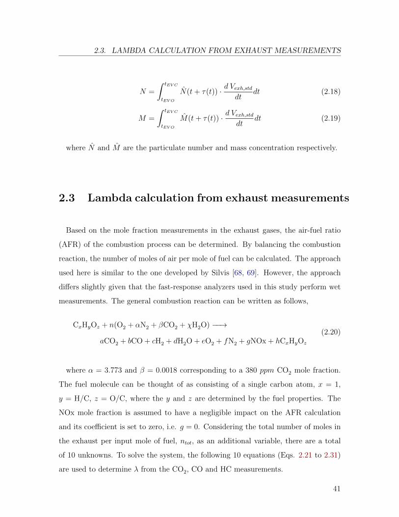
Lam
bda
/ -
0.5
1.0
1.5
2.0
2.5
Cycle number / -1 4 7 10 13 16 19
Lambda sensor Calculation
Figure 2-5: Calculated and measured λ during crank-start
The calculation of the AFR by means of the exhaust emissions measurements with
fast analyzers provides certain advantages over the direct measurement of the AFR
with a lambda sensor for crank start studies. First, the response time of a fully
warmed-up lambda sensor is on the order of 100 ms, that is, significantly slower
than the response time of the fast analyzers. Second, the lambda sensor is placed
sufficiently downstream of the exhaust line to allow for a correct temperature of
operation and to allow exhaust sampling from all cylinders, making it unsuitable
for cycle-resolved analysis of the crank-start process. Finally, the high HC emissions
during crank-start affect the characteristics of the diffusion layer of the oxygen sensor,
causing a lean shift in the measurement [5]. A typical trace for the calculated and
measured λ during the crank-start process can be seen in Fig. 2-5.
44
2.4. ENERGY CONVERSION ANALYSIS
2.4 Energy Conversion Analysis
2.4.1 Energy accounting from mole fraction measurements
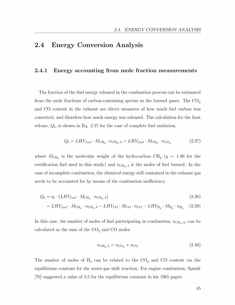
The fraction of the fuel energy released in the combustion process can be estimated
from the mole fractions of carbon-containing species in the burned gases. The CO2
and CO content in the exhaust are direct measures of how much fuel carbon was
converted, and therefore how much energy was released. The calculation for the heat
release, Qb, is shown in Eq. 2.37 for the case of complete fuel oxidation,
Qb = LHVfuel ·MCHy · nCHy , b = LHVfuel ·MCHy · nCO2(2.37)
where MCHy is the molecular weight of the hydrocarbon CHy (y = 1.86 for the
certification fuel used in this study) and nCHy , b is the moles of fuel burned. In the
case of incomplete combustion, the chemical energy still contained in the exhaust gas
needs to be accounted for by means of the combustion inefficiency.
Qb = ηc · (LHVfuel ·MCHy · nCHy , b) (2.38)
= LHVfuel ·MCHy · nCHy , b − LHVCO ·MCO · nCO − LHVH2·MH2
· nH2(2.39)
In this case, the number of moles of fuel participating in combustion, nCHy , b, can be
calculated as the sum of the CO2 and CO moles.
nCHy , b = nCO2+ nCO (2.40)
The number of moles of H2 can be related to the CO2 and CO content via the
equilibrium constant for the water-gas shift reaction. For engine combustion, Spindt
[70] suggested a value of 3.5 for the equilibrium constant in his 1965 paper.
45
CHAPTER 2. METHODOLOGY
nCO · nH2O
nCO2· nH2
= KWGSR (2.41)
The hydrogen mole balance provides the remaining piece of information to relate
the CO2 and CO content to the amount of H2 present in the burned gases.
y · nCHy , b = y · (nCO2+ nCO) = 2 · nH2O
+ 2 · nH2(2.42)
Combining Eqs. 2.41 and 2.42 gives:
nH2=y
2·
(nCO2+ nCO) · nCO
K · nCO2+ nCO
(2.43)
For a 1st cycle analysis, care must be taken to include the residual gases, with its
respective CO2, CO and H2 content as part of the products. For the subsequent cycles,
the residual gas fraction before and after combustion are similar, and therefore it is
not necessary to account them as product of the combustion. For a 1st cycle analysis:
ni = ni, Exh + ni, Res (2.44)
ni, Res =
(xi ·
p · VRu · T
)∣∣∣∣EV C
(2.45)
2.4.2 Heat release rate analysis
A first law analysis based on the in-cylinder pressure measurement provides crank-
angle resolved data on the heat release of the combustion process. Assuming a closed
system, the first law can be expressed as shown in Eq. 2.46,
δQb = dU + δW + δQwall (2.46)
46
2.4. ENERGY CONVERSION ANALYSIS
where δQb is the incremental heat release, dU represents the change in internal
energy of the cylinder content, δW is the change in work and δQwall is the heat
transfer to the combustion chamber walls. The work term is calculated from the
cylinder pressure and the piston position:
δW = p · dV (2.47)
Under the ideal gas assumption, the change in internal energy of the closed system can
be expressed using only the pressure and volume data (Eq. 2.48). Upon substitution,
Eq. 2.46 transforms into Eq. 2.49,
dU = m · cv · dT =pV
R· cv ·
dT
T=pV
R· cv · (
dp
p+dV
V) (2.48)
δQb =pV
R· cv · (
dp
p+dV
V) + p · dV =
cvR· V · dp+
cv +R
R· p · dV + δQwall (2.49)
where cv and R are the constant volume heat capacity of the gas and the ideal
gas constant respectively. Following an approach similar to Gatowski et al. [26], the
expression above can be manipulated algebraically to express the heat release rate as
a function of the pressure, volume, and their time derivatives;
dQb
dt=
1
γ − 1· V · dp
dt+
γ
γ − 1· p · dV
dt+dQwall
dt(2.50)
where γ is the heat capacity ratio cp/cv. For the calculation of the total heat release,
Eq. 2.50 can be integrated from the start of combustion (SoC) until the opening of
the exhaust valve, i.e. when the system stops being closed.
Qb = mCHy , b ·LHVfuel =
∫ tEV O
tSoC
(1
γ − 1·V · dp
dt+
γ
γ − 1· p · dV
dt+dQwall
dt
)dt (2.51)
47
CHAPTER 2. METHODOLOGY
The final task is to estimate the heat capacity ratio γ and the heat transfer rate
to the combustion chamber walls. The correlation used for estimating of the heat
capacity ratio as a function of temperature for gasoline mixtures was proposed by
Brunt et al. [3] as;
γ = 1.338− 6.0× 10⁻⁵ · T + 1.0× 10⁻⁸ · T 2 (2.52)
where T is the charge temperature in K estimated from the pressure and volume
data. The heat transfer rate was estimated using Woschni’s approach [77] for the
calculation of the heat transfer coefficient h. The model is shown in Eq. 2.53.
h = 0.013 · d−0.2 · p0.8 · T−0.53 · w0.8 (2.53)
In Eq. 2.53, w is an estimate of heat-transfer-relevant gas speed as a function of
engine speed and the cylinder pressure, is defined as follows:
w = C1 · cm + C2 ·Vd · TIV CpIV C · VIV C
· (p− pmot) (2.54)
with the mean piston speed cm in ms
calculated as a function of the engine speed
and stroke. Woschni proposed for gasoline engines that C1 = 2.28 for compression
and expansion strokes and C2 = 3.24× 10⁻³ msec·K .
Lejsek et al. [49] showed that the Woschni model results in a overestimation of the
wall heat flux at the low engine speeds observed during crank-start. Therefore, they
proposed and validated a correction for the effective gas velocity w (Eq. 2.55) for low
engine speeds between 150− 1000 rpm. Gstart and Bstart are defined in Eq. 2.56.
48
2.4. ENERGY CONVERSION ANALYSIS
w = Gstart · C1 · cm +Bstart · C2 ·Vd · TIV CpIV C · VIV C
· (p− pmot) (2.55)
Gstart = 2.14− 0.795 · cm,k +293.15
Twalland Bstart =
1
4· (VcV
)1/3 (2.56)
Where cm,k is the mean piston speed during the compression stroke, and Vc is the
clearance volume. Having estimated the heat transfer coefficient, the heat transfer
rate can be calculated as a function of the exposed cylinder surface area Acyl, the
charge temperature T and the wall temperature Twall.
dQwall
dt= Acyl(t) · h(t) ·
(T (t)− Twall
)(2.57)
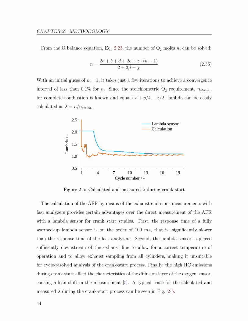
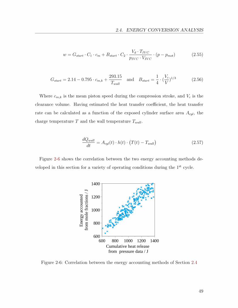
Figure 2-6 shows the correlation between the two energy accounting methods de-
veloped in this section for a variety of operating conditions during the 1st cycle.
Ene
rgy
acco
unte
d fr
om m
ole
frac
tion
s / J
600
800
1000
1200
1400
Cumulative heat release from pressure data / J
600 800 1000 1200 1400
Figure 2-6: Correlation between the energy accounting methods of Section 2.4
49

– Intentionally left blank –
Chapter 3
Fuel accounting for the first cycle
As a part of the systematic study of the emissions in the cold-start processes of a
GDI engine, this chapter deals with the fuel carbon pathway in the 1st cycle of the cold
crank-start process. Since the associated particulate emissions are negligibly small
in terms of the fuel carbon mass, they are not included in the following analysis.
The topic of particle emissions during the 1st cycle is addressed in Chapter 4. A
carbon accounting analysis is used to deconstruct the amounts of fuel participating
in combustion, being exhausted as HC emissions, staying in the combustion chamber
for the 2nd combustion event, and being absorbed by the oil or lost through blow-
by. The engine is fired for a single cycle in one cylinder at cold start condition
(20◦C). The fuel carbon is accounted from CO2, CO, and HC measurements using
fast response analyzers. The parameters studied are the fuel enrichment, the injection
and ignition timing, the intake and fuel pressures, and the cranking speed. Substantial
fuel enrichment is needed to produce stable combustion in the 1st cycle. A share of
the fuel is available for the 2nd cycle and a share goes into the oil and crank case.
Part of the results presented in this chapter have been published in the International
Journal of Engine Research [61].
51
CHAPTER 3. FUEL ACCOUNTING FOR THE FIRST CYCLE
3.1 Experiments description
The engine crank-start is a highly transient process, with engine speed variations
of up to 200 rpm within a combustion cycle. The sequence of events depends heavily
on the 1st combustion event. Therefore, as an initial step to fully understand the
cold-cranking emissions, the fuel pathway of 1st firing cycle is examined in detail.
To recreate the cold-start conditions, the engine coolant, engine oil, fuel, and intake
air temperatures were kept at 20◦C. The temperatures of the engine components
under steady-state motoring at 280 rpm were simulated using a commercially available
software; the piston temperature distribution is shown in Fig. 3-1. The cylinder liner
temperature stabilizes at a value of 25◦C, the piston crown temperature at 29◦C, and
the piston skirt at 26◦C under the steady-state motoring conditions. The camshaft
timing was kept at its parked position, corresponding to a negative valve overlap
(NVO) of 20◦CA.
Figure 3-1: Simulated piston temperature performed with GT-Power under steadystate motoring at 280 rpm and 20◦C coolant temperature
52
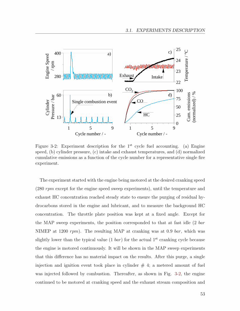
3.1. EXPERIMENTS DESCRIPTION
Eng
ine
Spe
ed
/ rp
m
280
400 a)C
ylin
der
Pre
ssur
e /
bar
13
60
Cycle number / -1 5 9
Single combustion event
b)
Cum
. em
issi
ons
(nor
mal
ized
) /
%
0
25
50
75
100
Cycle number / -1 5 9
CO2
CO
HC
d)
Tem
pera
ture
/ °
C
22
23
24
25c)
Exhaust Intake
Figure 3-2: Experiment description for the 1st cycle fuel accounting. (a) Enginespeed, (b) cylinder pressure, (c) intake and exhaust temperatures, and (d) normalizedcumulative emissions as a function of the cycle number for a representative single fireexperiment.
The experiment started with the engine being motored at the desired cranking speed
(280 rpm except for the engine speed sweep experiments), until the temperature and
exhaust HC concentration reached steady state to ensure the purging of residual hy-
drocarbons stored in the engine and lubricant, and to measure the background HC
concentration. The throttle plate position was kept at a fixed angle. Except for
the MAP sweep experiments, the position corresponded to that at fast idle (2 bar
NIMEP at 1200 rpm). The resulting MAP at cranking was at 0.9 bar, which was
slightly lower than the typical value (1 bar) for the actual 1st cranking cycle because
the engine is motored continuously. It will be shown in the MAP sweep experiments
that this difference has no material impact on the results. After this purge, a single
injection and ignition event took place in cylinder # 4; a metered amount of fuel
was injected followed by combustion. Thereafter, as shown in Fig. 3-2, the engine
continued to be motored at cranking speed and the exhaust stream composition and
53
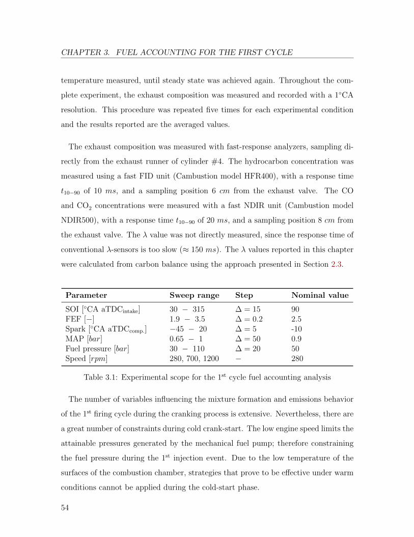
CHAPTER 3. FUEL ACCOUNTING FOR THE FIRST CYCLE
temperature measured, until steady state was achieved again. Throughout the com-
plete experiment, the exhaust composition was measured and recorded with a 1◦CA
resolution. This procedure was repeated five times for each experimental condition
and the results reported are the averaged values.
The exhaust composition was measured with fast-response analyzers, sampling di-
rectly from the exhaust runner of cylinder #4. The hydrocarbon concentration was
measured using a fast FID unit (Cambustion model HFR400), with a response time
t10−90 of 10 ms, and a sampling position 6 cm from the exhaust valve. The CO
and CO2 concentrations were measured with a fast NDIR unit (Cambustion model
NDIR500), with a response time t10−90 of 20 ms, and a sampling position 8 cm from
the exhaust valve. The λ value was not directly measured, since the response time of
conventional λ-sensors is too slow (≈ 150 ms). The λ values reported in this chapter
were calculated from carbon balance using the approach presented in Section 2.3.
Parameter Sweep range Step Nominal value
SOI [◦CA aTDCintake] 30 − 315 ∆ = 15 90FEF [−] 1.9 − 3.5 ∆ = 0.2 2.5Spark [◦CA aTDCcomp.] −45 − 20 ∆ = 5 -10MAP [bar] 0.65 − 1 ∆ = 50 0.9Fuel pressure [bar] 30 − 110 ∆ = 20 50Speed [rpm] 280, 700, 1200 − 280
Table 3.1: Experimental scope for the 1st cycle fuel accounting analysis
The number of variables influencing the mixture formation and emissions behavior
of the 1st firing cycle during the cranking process is extensive. Nevertheless, there are
a great number of constraints during cold crank-start. The low engine speed limits the
attainable pressures generated by the mechanical fuel pump; therefore constraining
the fuel pressure during the 1st injection event. Due to the low temperature of the
surfaces of the combustion chamber, strategies that prove to be effective under warm
conditions cannot be applied during the cold-start phase.
54
3.2. FUEL ACCOUNTING METHODOLOGY
The fuel accounting analysis was focused in six different engine parameters using
a one-variable-at-a-time approach. The variables studied are: First cycle fuel enrich-
ment factor (FEF, see Eq. 3.1), injection timing (SOI), spark timing, 1st cycle intake
manifold pressure (MAP), fuel pressure and engine cranking speed. The parameters
tested are summarized in Table 3.1.
Since not all the injected fuel goes into the charge mixture, a large amount of
fuel has to be injected to achieve stable combustion in the 1st cycle. To quantify
the amount of additional fuel required, a fuel enrichment factor (FEF) based on a
speed-density calibration is defined.
FEF =mf,cyl · AFRstoich.
Vcyl · ηvol · ρint(3.1)
3.2 Fuel accounting methodology
3.2.1 Carbon accounting
In order to understand the fuel pathway during the 1st combustion cycle a fuel
carbon accounting analysis is performed. The goal of this analysis is to quantify the
amount of fuel participating in combustion, the fuel carbon fraction being exhausted
as unburned hydrocarbons, and the fraction that cannot be accounted for, represent-
ing primarily the engine oil dilution by fuel and the blow-by losses. The analysis is
done by translating the fuel and exhaust mass flows to equivalent carbon mass flows,
and then performing a control volume analysis around the cylinder.
mC, in = mC, out + mC, Engine (3.2)
55
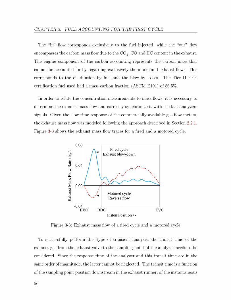
CHAPTER 3. FUEL ACCOUNTING FOR THE FIRST CYCLE
The “in” flow corresponds exclusively to the fuel injected, while the “out” flow
encompasses the carbon mass flow due to the CO2, CO and HC content in the exhaust.
The engine component of the carbon accounting represents the carbon mass that
cannot be accounted for by regarding exclusively the intake and exhaust flows. This
corresponds to the oil dilution by fuel and the blow-by losses. The Tier II EEE
certification fuel used had a mass carbon fraction (ASTM E191) of 86.5%.
In order to relate the concentration measurements to mass flows, it is necessary to
determine the exhaust mass flow and correctly synchronize it with the fast analyzers
signals. Given the slow time response of the commercially available gas flow meters,
the exhaust mass flow was modeled following the approach described in Section 2.2.1.
Figure 3-3 shows the exhaust mass flow traces for a fired and a motored cycle.
0.00
0.04
0.08
Piston Position / -EVO EVC
Fired cycleExhaust blow-down
Motored cycleReverse flowE
xhau
st M
ass
Flow
Rat
e / k
g/s
-0.04
0.00
0.04
0.08
BDC
Figure 3-3: Exhaust mass flow of a fired cycle and a motored cycle
To successfully perform this type of transient analysis, the transit time of the
exhaust gas from the exhaust valve to the sampling point of the analyzer needs to be
considered. Since the response time of the analyzer and this transit time are in the
same order of magnitude, the latter cannot be neglected. The transit time is a function
of the sampling point position downstream in the exhaust runner, of the instantaneous
56
3.2. FUEL ACCOUNTING METHODOLOGY
exhaust mass flow, and of the exhaust gas density. Following the method described
in Section 2.2.2, the calculated mass flow and the exhaust temperature can be used
to determine the appropriate transit delay correction to the concentration signals
from the fast analyzers. Once the exhaust mass flow and the concentration signals
are synchronized, the carbon mass flow due to each constituent can be calculated by
multiplying the measured wet mole fraction of the component by the exhaust molar
flow (using MWexh = 28.9 g/mol) and the molecular weight of carbon.
mC,y = xy ·mexh
MWexh
·MWC (3.3)
For the motored cycles after the single-cycle firing, the cylinder pressure is lower
than the exhaust pressure when the exhaust valve opens. Thus, as shown in Fig.
3-3, the exhaust flow is initially backwards until the pressure reaches equilibrium and
the positive displacement flow begins. By measuring the HC mole fraction during
the reverse flow, it is possible to account for the HC content flowing from the ex-
haust manifold into the cylinder during this period, thus avoiding double-counting of
emissions for the reverse flow in the motored cycles.
The goal of the experiment is to deconstruct the pathways for the single-cycle-
injected fuel and to examine how the engine parameters affect the pathways. As
such, the individual carbon exhaust mass flows due to each component (CO2, CO,
and HC) are integrated for the firing and the subsequent motoring cycles, and the
cycle-resolved results are summarized in three sets of numbers:
1. The first set is the HC emissions, respectively, of the 1st, 2nd, and sum of the
3rd-and-beyond cycles. The 1st (firing) cycle HC emissions give information
of the emission performance; the 2nd (motoring) cycle HC emissions indicate
the amount of the in-cylinder retained fuel from the 1st combustion event that
would contribute to the combustible mixture of the 2nd cycle. The HC emissions
57
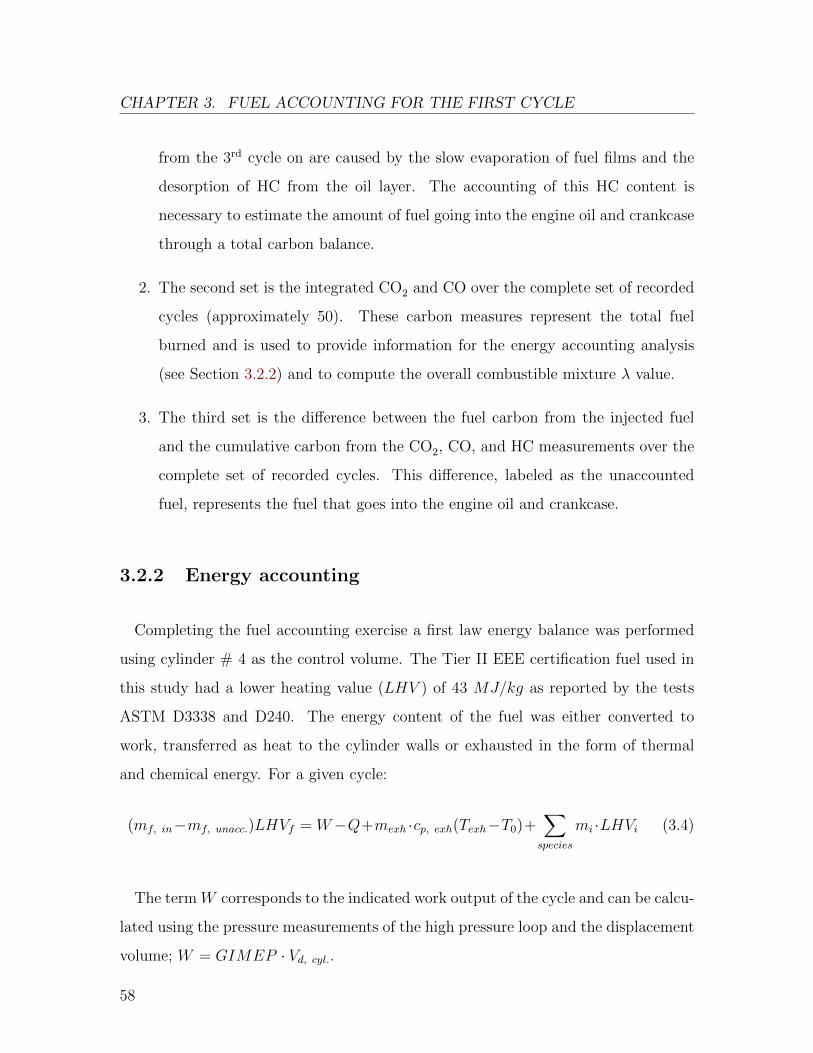
CHAPTER 3. FUEL ACCOUNTING FOR THE FIRST CYCLE
from the 3rd cycle on are caused by the slow evaporation of fuel films and the
desorption of HC from the oil layer. The accounting of this HC content is
necessary to estimate the amount of fuel going into the engine oil and crankcase
through a total carbon balance.
2. The second set is the integrated CO2 and CO over the complete set of recorded
cycles (approximately 50). These carbon measures represent the total fuel
burned and is used to provide information for the energy accounting analysis
(see Section 3.2.2) and to compute the overall combustible mixture λ value.
3. The third set is the difference between the fuel carbon from the injected fuel
and the cumulative carbon from the CO2, CO, and HC measurements over the
complete set of recorded cycles. This difference, labeled as the unaccounted
fuel, represents the fuel that goes into the engine oil and crankcase.
3.2.2 Energy accounting
Completing the fuel accounting exercise a first law energy balance was performed
using cylinder # 4 as the control volume. The Tier II EEE certification fuel used in
this study had a lower heating value (LHV ) of 43 MJ/kg as reported by the tests
ASTM D3338 and D240. The energy content of the fuel was either converted to
work, transferred as heat to the cylinder walls or exhausted in the form of thermal
and chemical energy. For a given cycle:
(mf, in−mf, unacc.)LHVf = W−Q+mexh ·cp, exh(Texh−T0)+∑species
mi ·LHVi (3.4)
The term W corresponds to the indicated work output of the cycle and can be calcu-
lated using the pressure measurements of the high pressure loop and the displacement
volume; W = GIMEP · Vd, cyl..
58
3.3. INJECTION TIMING SWEEP
The term Q refers to the heat transfer to the combustion chamber walls, and
ultimately to the engine coolant. Its calculation is based on the classical approach
presented by Woschni in the 1960’s [77] with an appropiate correction for low engine
speed proposed by Lejsek et al. [49]. The details of the approach can be found in
Section 2.4.2.
The terms mexh ·cp, exh ·(Texh−T0) and∑
speciesmi ·LHVi correspond to the sensible
and chemical energy of the exhaust gases respectively. Due to the slow response
time of thermocouples, measuring accurately the gas temperature of a single exhaust
stroke was not possible. The thermal enthalpy was then calculated as the difference
between the total heat release as calculated based on the fuel conversion to CO2 and
CO (Section 2.4.2) and the work and heat transfer terms. The chemical component of
the enthalpy was calculated using the fuel carbon accounting analysis and the lower
heating value (LHVi) of the exhausted species. The species considered were total HC,
CO and H2. The H2 content of the exhaust was not measured directly but calculated
using the approach presented in Section 2.3.
Lastly, as mentioned in the previous section, a significant part of the injected fuel
is dissolved into the oil layer or lost to the crankcase due to blow-by. The term
mf, unacc. · LHVf represents the energy content of this lost fuel.
3.3 Injection timing sweep
The injection timing has a strong influence on the mixture formation process. As a
general rule, under warm operation conditions, early injection timings result in more
homogeneous mixtures, while late injection timings result in higher heterogeneity and
charge turbulence prior to ignition [39]. On the other hand, for side-mounted injectors
and at cold engine temperatures, the injection timing also determines the amount and
59
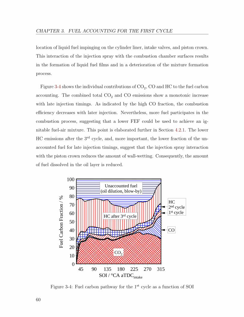
CHAPTER 3. FUEL ACCOUNTING FOR THE FIRST CYCLE
location of liquid fuel impinging on the cylinder liner, intake valves, and piston crown.
This interaction of the injection spray with the combustion chamber surfaces results
in the formation of liquid fuel films and in a deterioration of the mixture formation
process.
Figure 3-4 shows the individual contributions of CO2, CO and HC to the fuel carbon
accounting. The combined total CO2 and CO emissions show a monotonic increase
with late injection timings. As indicated by the high CO fraction, the combustion
efficiency decreases with later injection. Nevertheless, more fuel participates in the
combustion process, suggesting that a lower FEF could be used to achieve an ig-
nitable fuel-air mixture. This point is elaborated further in Section 4.2.1. The lower
HC emissions after the 3rd cycle, and, more important, the lower fraction of the un-
accounted fuel for late injection timings, suggest that the injection spray interaction
with the piston crown reduces the amount of wall-wetting. Consequently, the amount
of fuel dissolved in the oil layer is reduced.
Fue
l Car
bon
Fra
ctio
n /
%
0
10
20
30
40
50
60
70
80
90
100
SOI / °CA aTDCintake
45 90 135 180 225 270 315
HC after 3rd cycle
Unaccounted fuel(oil dilution, blow-by)
CO2
CO
HC 2nd cycle1st cycle
Figure 3-4: Fuel carbon pathway for the 1st cycle as a function of SOI
60
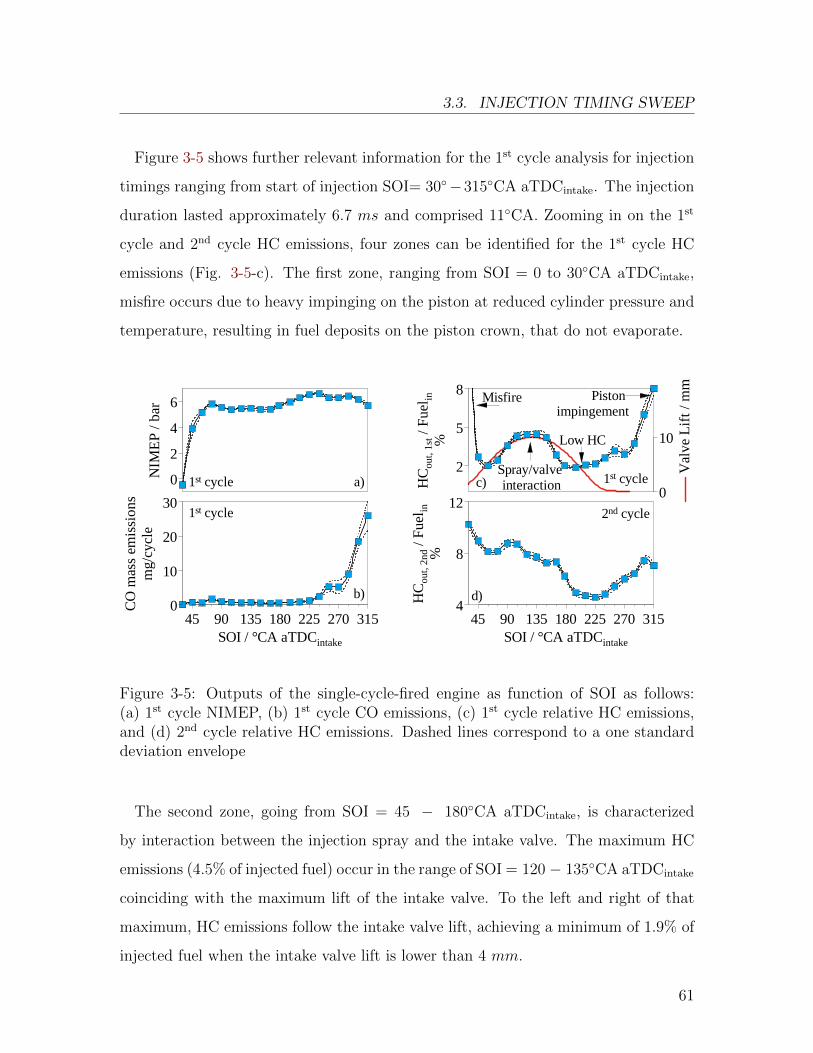
3.3. INJECTION TIMING SWEEP
Figure 3-5 shows further relevant information for the 1st cycle analysis for injection
timings ranging from start of injection SOI= 30◦−315◦CA aTDCintake. The injection
duration lasted approximately 6.7 ms and comprised 11◦CA. Zooming in on the 1st
cycle and 2nd cycle HC emissions, four zones can be identified for the 1st cycle HC
emissions (Fig. 3-5-c). The first zone, ranging from SOI = 0 to 30◦CA aTDCintake,
misfire occurs due to heavy impinging on the piston at reduced cylinder pressure and
temperature, resulting in fuel deposits on the piston crown, that do not evaporate.
Low HC
Piston impingement
Spray/valve interaction
Misfire
Val
ve L
ift /
mm
0
10H
Cou
t, 1
st /
Fue
l in%
2
5
8
c) 1st cycle
HC
out,
2nd /
Fue
l in%
4
8
12
SOI / °CA aTDCintake
45 90 135 180 225 270 315
2nd cycle
d)
CO
mas
s em
issi
on
sm
g/cy
cle
0
10
20
30
SOI / °CA aTDCintake
45 90 135 180 225 270 315
b)
1st cycle
NIM
EP
/ b
ar
0
2
4
6
a)1st cycle
Figure 3-5: Outputs of the single-cycle-fired engine as function of SOI as follows:(a) 1st cycle NIMEP, (b) 1st cycle CO emissions, (c) 1st cycle relative HC emissions,and (d) 2nd cycle relative HC emissions. Dashed lines correspond to a one standarddeviation envelope
The second zone, going from SOI = 45 − 180◦CA aTDCintake, is characterized
by interaction between the injection spray and the intake valve. The maximum HC
emissions (4.5% of injected fuel) occur in the range of SOI = 120 − 135◦CA aTDCintake
coinciding with the maximum lift of the intake valve. To the left and right of that
maximum, HC emissions follow the intake valve lift, achieving a minimum of 1.9% of
injected fuel when the intake valve lift is lower than 4 mm.
61
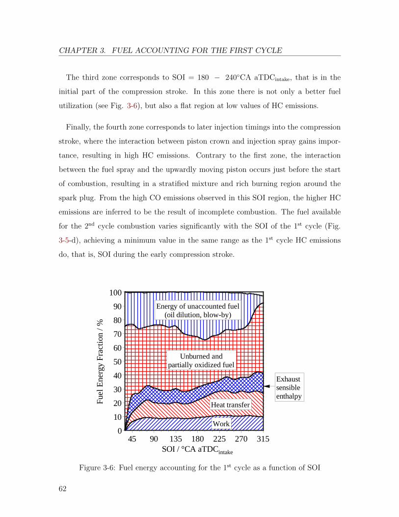
CHAPTER 3. FUEL ACCOUNTING FOR THE FIRST CYCLE
The third zone corresponds to SOI = 180 − 240◦CA aTDCintake, that is in the
initial part of the compression stroke. In this zone there is not only a better fuel
utilization (see Fig. 3-6), but also a flat region at low values of HC emissions.
Finally, the fourth zone corresponds to later injection timings into the compression
stroke, where the interaction between piston crown and injection spray gains impor-
tance, resulting in high HC emissions. Contrary to the first zone, the interaction
between the fuel spray and the upwardly moving piston occurs just before the start
of combustion, resulting in a stratified mixture and rich burning region around the
spark plug. From the high CO emissions observed in this SOI region, the higher HC
emissions are inferred to be the result of incomplete combustion. The fuel available
for the 2nd cycle combustion varies significantly with the SOI of the 1st cycle (Fig.
3-5-d), achieving a minimum value in the same range as the 1st cycle HC emissions
do, that is, SOI during the early compression stroke.
Fue
l Ene
rgy
Fra
ctio
n /
%
0
10
20
30
40
50
60
70
80
90
100
SOI / °CA aTDCintake
45 90 135 180 225 270 315
Work
Heat transfer
Unburned andpartially oxidized fuel
Energy of unaccounted fuel(oil dilution, blow-by)
Exhaust sensibleenthalpy
Figure 3-6: Fuel energy accounting for the 1st cycle as a function of SOI
62
3.3. INJECTION TIMING SWEEP
Figure 3-6 shows the contributions of work, heat transfer, exhaust enthalpy and lost
fuel to the fuel energy accounting. The amount of energy converted to work, in other
words the first law efficiency, lies between 8 and 10%. Using the 1st cycle NIMEP
as a measure of the work output the following analysis can be made. As shown in
Fig. 3-5-a, the NIMEP increases from 0 bar at SOI= 30◦CA aTDCintake (misfire)
to 6 bar at SOI= 75◦CA aTDCintake. This zone corresponds to heavy impinging
on the piston for injection timings lower than SOI= 75◦CA aTDCintake. As the
piston moves downward and the impingement decreases, the NIMEP stays relatively
constant for injections during the intake stroke. For compression stroke injections,
the higher in-cylinder pressure reduces the injection spray penetration, allowing for
a better mixture formation and increased fraction of fuel evaporated. Consequently,
an increase in NIMEP for SOI up to 225◦CA aTDCintake is observed. Up to this
injection timing the homogeneity of the mixture stays relatively constant, as can
be seen by the constant low values of the emitted CO. The NIMEP trend becomes
flat, while the mixture becomes increasingly heterogeneous. At the injection timing
SOI = 285◦CA aTDCintake the fuel spray impinges again on the piston crown. The
result is a very heterogeneous and rich mixture around the spark plug, characterized
by high CO production (Fig. 3-5-b) and slightly lower NIMEP.
The heat transfer to the engine walls accounts for 10 to 18% of the total fuel
energy. For injection timings during the intake stroke, the fraction of the fuel energy
lost as heat transfer to the coolant between 10 and 12%. As the SOI moves into the
compression stroke the heat transfer increases up to a maximum of 18% (≈ 570 J) at
SOI = 300◦CA aTDCintake. The heat transfer is a function of the amount and timing
of the heat release rate. As argued previously, as the injection timings is delayed, more
fuel takes part in combustion and the amount of heat release increases. Furthermore,
as shown in Fig. 3-7, as the injection timing is delayed in the compression stroke and
the mixture becomes increasingly stratified, the flame development and burn duration
are shorter and the peak of heat release is shifted to an earlier point.
63
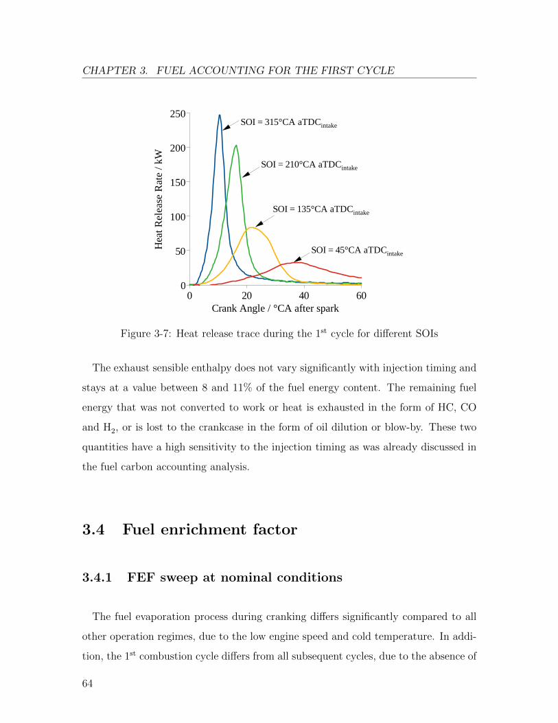
CHAPTER 3. FUEL ACCOUNTING FOR THE FIRST CYCLE
Hea
t R
ele
ase
Rat
e /
kW
0
50
100
150
200
250
Crank Angle / °CA after spark0 20 40 60
SOI = 315°CA aTDCintake
SOI = 45°CA aTDCintake
SOI = 210°CA aTDCintake
SOI = 135°CA aTDCintake
Figure 3-7: Heat release trace during the 1st cycle for different SOIs
The exhaust sensible enthalpy does not vary significantly with injection timing and
stays at a value between 8 and 11% of the fuel energy content. The remaining fuel
energy that was not converted to work or heat is exhausted in the form of HC, CO
and H2, or is lost to the crankcase in the form of oil dilution or blow-by. These two
quantities have a high sensitivity to the injection timing as was already discussed in
the fuel carbon accounting analysis.
3.4 Fuel enrichment factor
3.4.1 FEF sweep at nominal conditions
The fuel evaporation process during cranking differs significantly compared to all
other operation regimes, due to the low engine speed and cold temperature. In addi-
tion, the 1st combustion cycle differs from all subsequent cycles, due to the absence of
64
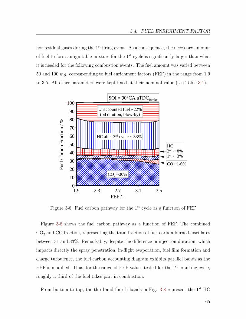
3.4. FUEL ENRICHMENT FACTOR
hot residual gases during the 1st firing event. As a consequence, the necessary amount
of fuel to form an ignitable mixture for the 1st cycle is significantly larger than what
it is needed for the following combustion events. The fuel amount was varied between
50 and 100 mg, corresponding to fuel enrichment factors (FEF) in the range from 1.9
to 3.5. All other parameters were kept fixed at their nominal value (see Table 3.1).
Fue
l Car
bon
Fra
ctio
n /
%
0
10
20
30
40
50
60
70
80
90
100
FEF / -1.9 2.3 2.7 3.1 3.5
CO2 ~30%
Unaccounted fuel ~22%(oil dilution, blow-by)
HC after 3rd cycle ~ 33%
HC 2nd ~ 8%1st ~ 3%
CO ~1-6%
SOI = 90°CA aTDCintake
Figure 3-8: Fuel carbon pathway for the 1st cycle as a function of FEF
Figure 3-8 shows the fuel carbon pathway as a function of FEF. The combined
CO2 and CO fraction, representing the total fraction of fuel carbon burned, oscillates
between 31 and 33%. Remarkably, despite the difference in injection duration, which
impacts directly the spray penetration, in-flight evaporation, fuel film formation and
charge turbulence, the fuel carbon accounting diagram exhibits parallel bands as the
FEF is modified. Thus, for the range of FEF values tested for the 1st cranking cycle,
roughly a third of the fuel takes part in combustion.
From bottom to top, the third and fourth bands in Fig. 3-8 represent the 1st HC
65
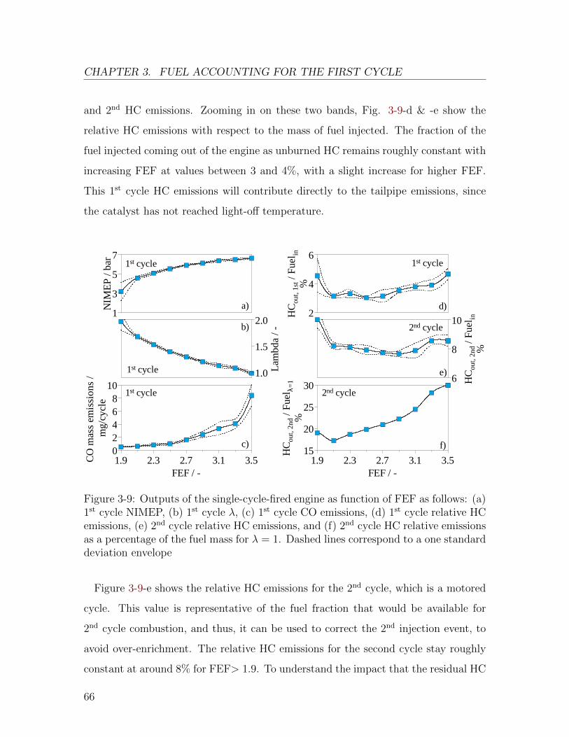
CHAPTER 3. FUEL ACCOUNTING FOR THE FIRST CYCLE
and 2nd HC emissions. Zooming in on these two bands, Fig. 3-9-d & -e show the
relative HC emissions with respect to the mass of fuel injected. The fraction of the
fuel injected coming out of the engine as unburned HC remains roughly constant with
increasing FEF at values between 3 and 4%, with a slight increase for higher FEF.
This 1st cycle HC emissions will contribute directly to the tailpipe emissions, since
the catalyst has not reached light-off temperature.
HC
out,
2nd
/ Fue
l λ=1
%
15
20
25
30
FEF / -1.9 2.3 2.7 3.1 3.5
2nd cycle
f)
NIM
EP
/ bar
1
3
5
7
a)
1st cycle
HC
out,
1st /
Fue
l in%
2
4
6
d)
1st cycle
HC
out,
2nd
/ Fue
l in%
6
8
10
e)
2nd cycle
Lam
bda
/ -
1.0
1.5
2.0b)
1st cycle
CO
mas
s em
issi
ons
/ m
g/cy
cle
02468
10
FEF / -1.9 2.3 2.7 3.1 3.5
c)
1st cycle
Figure 3-9: Outputs of the single-cycle-fired engine as function of FEF as follows: (a)1st cycle NIMEP, (b) 1st cycle λ, (c) 1st cycle CO emissions, (d) 1st cycle relative HCemissions, (e) 2nd cycle relative HC emissions, and (f) 2nd cycle HC relative emissionsas a percentage of the fuel mass for λ = 1. Dashed lines correspond to a one standarddeviation envelope
Figure 3-9-e shows the relative HC emissions for the 2nd cycle, which is a motored
cycle. This value is representative of the fuel fraction that would be available for
2nd cycle combustion, and thus, it can be used to correct the 2nd injection event, to
avoid over-enrichment. The relative HC emissions for the second cycle stay roughly
constant at around 8% for FEF> 1.9. To understand the impact that the residual HC
66
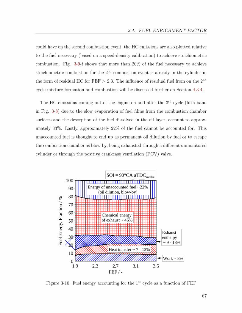
3.4. FUEL ENRICHMENT FACTOR
could have on the second combustion event, the HC emissions are also plotted relative
to the fuel necessary (based on a speed-density calibration) to achieve stoichiometric
combustion. Fig. 3-9-f shows that more than 20% of the fuel necessary to achieve
stoichiometric combustion for the 2nd combustion event is already in the cylinder in
the form of residual HC for FEF > 2.3. The influence of residual fuel from on the 2nd
cycle mixture formation and combustion will be discussed further on Section 4.3.4.
The HC emissions coming out of the engine on and after the 3rd cycle (fifth band
in Fig. 3-8) due to the slow evaporation of fuel films from the combustion chamber
surfaces and the desorption of the fuel dissolved in the oil layer, account to approx-
imately 33%. Lastly, approximately 22% of the fuel cannot be accounted for. This
unaccounted fuel is thought to end up as permanent oil dilution by fuel or to escape
the combustion chamber as blow-by, being exhausted through a different unmonitored
cylinder or through the positive crankcase ventilation (PCV) valve.
Fue
l Ene
rgy
Fra
ctio
n /
%
0
10
20
30
40
50
60
70
80
90
100
FEF / -1.9 2.3 2.7 3.1 3.5
Heat transfer ~ 7 - 13%
Energy of unaccounted fuel ~22%(oil dilution, blow-by)
Chemical energyof exhaust ~ 46%
Work ~ 8%
Exhaustenthalpy ~ 9 - 18%
SOI = 90°CA aTDCintake
Figure 3-10: Fuel energy accounting for the 1st cycle as a function of FEF
67
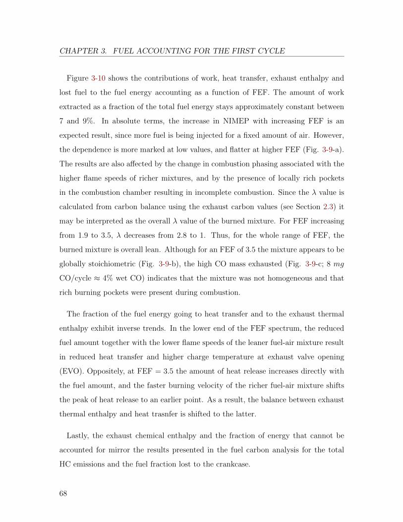
CHAPTER 3. FUEL ACCOUNTING FOR THE FIRST CYCLE
Figure 3-10 shows the contributions of work, heat transfer, exhaust enthalpy and
lost fuel to the fuel energy accounting as a function of FEF. The amount of work
extracted as a fraction of the total fuel energy stays approximately constant between
7 and 9%. In absolute terms, the increase in NIMEP with increasing FEF is an
expected result, since more fuel is being injected for a fixed amount of air. However,
the dependence is more marked at low values, and flatter at higher FEF (Fig. 3-9-a).
The results are also affected by the change in combustion phasing associated with the
higher flame speeds of richer mixtures, and by the presence of locally rich pockets
in the combustion chamber resulting in incomplete combustion. Since the λ value is
calculated from carbon balance using the exhaust carbon values (see Section 2.3) it
may be interpreted as the overall λ value of the burned mixture. For FEF increasing
from 1.9 to 3.5, λ decreases from 2.8 to 1. Thus, for the whole range of FEF, the
burned mixture is overall lean. Although for an FEF of 3.5 the mixture appears to be
globally stoichiometric (Fig. 3-9-b), the high CO mass exhausted (Fig. 3-9-c; 8 mg
CO/cycle ≈ 4% wet CO) indicates that the mixture was not homogeneous and that
rich burning pockets were present during combustion.
The fraction of the fuel energy going to heat transfer and to the exhaust thermal
enthalpy exhibit inverse trends. In the lower end of the FEF spectrum, the reduced
fuel amount together with the lower flame speeds of the leaner fuel-air mixture result
in reduced heat transfer and higher charge temperature at exhaust valve opening
(EVO). Oppositely, at FEF = 3.5 the amount of heat release increases directly with
the fuel amount, and the faster burning velocity of the richer fuel-air mixture shifts
the peak of heat release to an earlier point. As a result, the balance between exhaust
thermal enthalpy and heat trasnfer is shifted to the latter.
Lastly, the exhaust chemical enthalpy and the fraction of energy that cannot be
accounted for mirror the results presented in the fuel carbon analysis for the total
HC emissions and the fuel fraction lost to the crankcase.
68
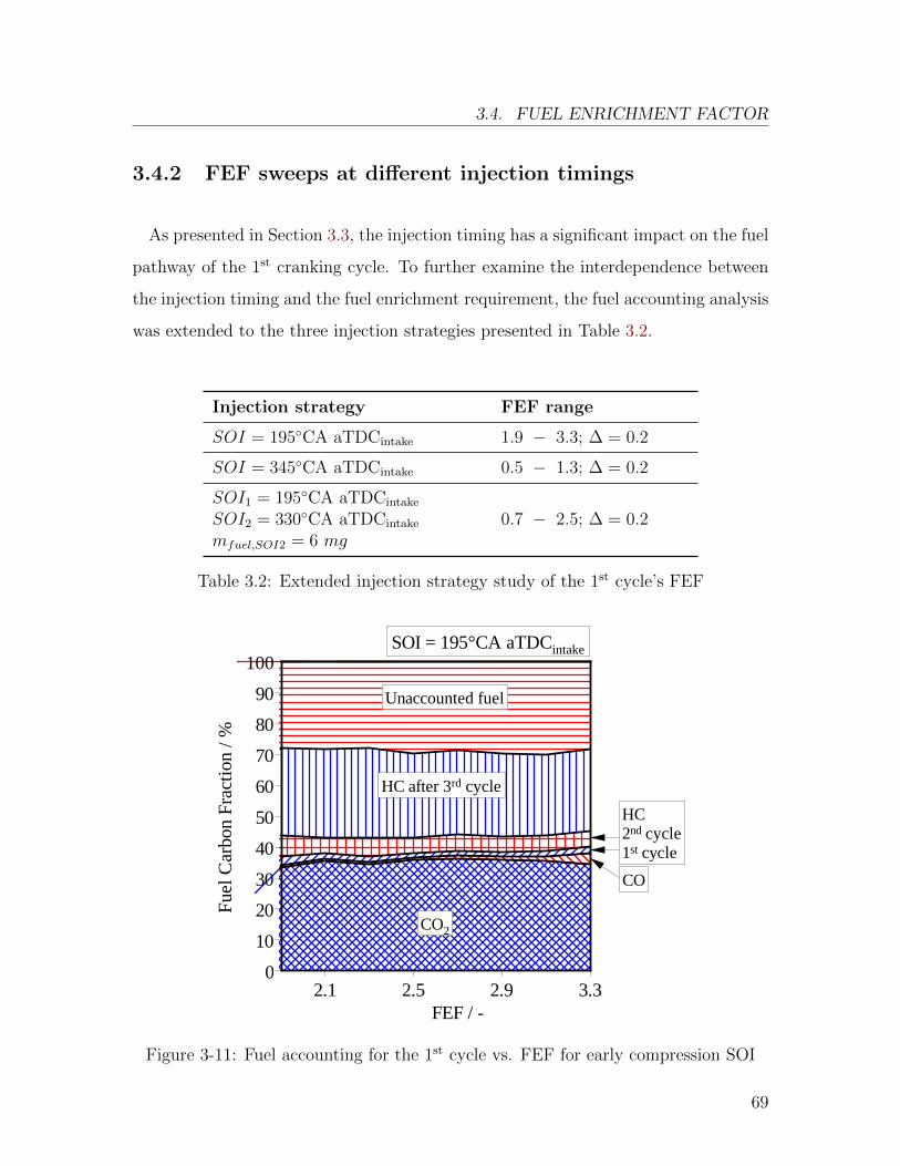
3.4. FUEL ENRICHMENT FACTOR
3.4.2 FEF sweeps at different injection timings
As presented in Section 3.3, the injection timing has a significant impact on the fuel
pathway of the 1st cranking cycle. To further examine the interdependence between
the injection timing and the fuel enrichment requirement, the fuel accounting analysis
was extended to the three injection strategies presented in Table 3.2.
Injection strategy FEF range
SOI = 195◦CA aTDCintake 1.9 − 3.3; ∆ = 0.2
SOI = 345◦CA aTDCintake 0.5 − 1.3; ∆ = 0.2
SOI1 = 195◦CA aTDCintake
SOI2 = 330◦CA aTDCintake 0.7 − 2.5; ∆ = 0.2mfuel,SOI2 = 6 mg
Table 3.2: Extended injection strategy study of the 1st cycle’s FEF
Fue
l Car
bon
Fra
ctio
n /
%
0
10
20
30
40
50
60
70
80
90
100
FEF / -2.1 2.5 2.9 3.3
CO2
Unaccounted fuel
HC after 3rd cycle
HC 2nd cycle1st cycle
CO
SOI = 195°CA aTDCintake
Figure 3-11: Fuel accounting for the 1st cycle vs. FEF for early compression SOI
69
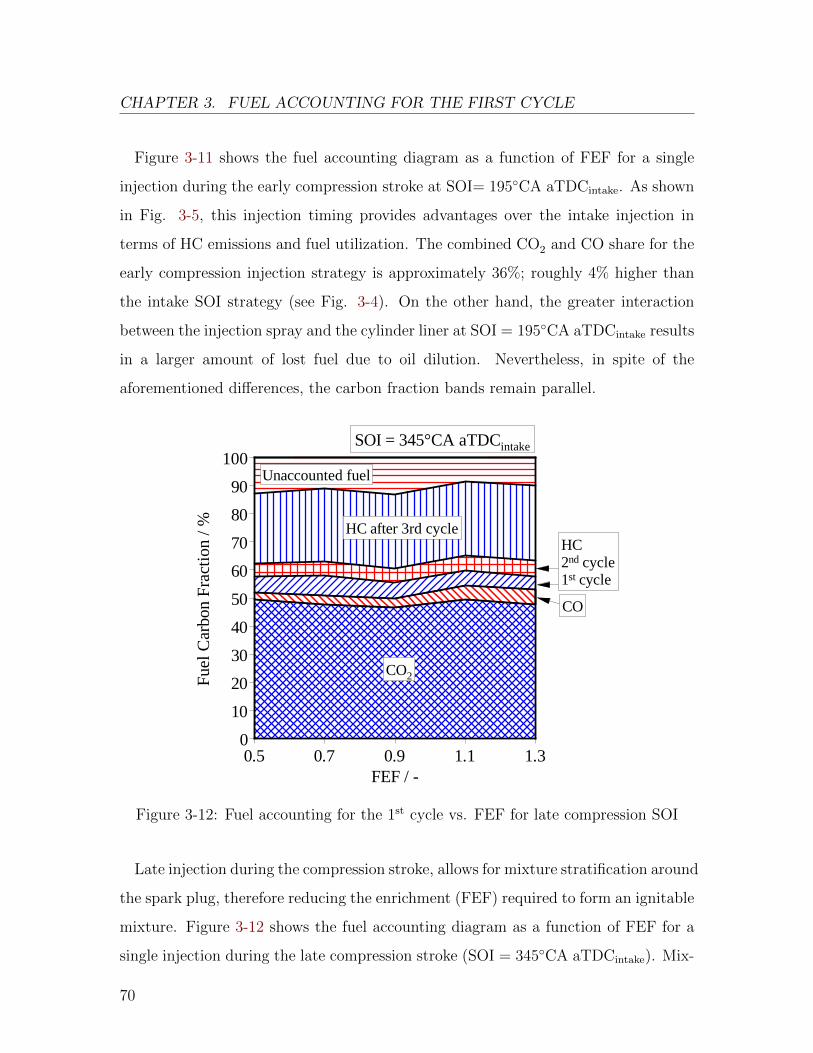
CHAPTER 3. FUEL ACCOUNTING FOR THE FIRST CYCLE
Figure 3-11 shows the fuel accounting diagram as a function of FEF for a single
injection during the early compression stroke at SOI= 195◦CA aTDCintake. As shown
in Fig. 3-5, this injection timing provides advantages over the intake injection in
terms of HC emissions and fuel utilization. The combined CO2 and CO share for the
early compression injection strategy is approximately 36%; roughly 4% higher than
the intake SOI strategy (see Fig. 3-4). On the other hand, the greater interaction
between the injection spray and the cylinder liner at SOI = 195◦CA aTDCintake results
in a larger amount of lost fuel due to oil dilution. Nevertheless, in spite of the
aforementioned differences, the carbon fraction bands remain parallel.
Fue
l Car
bon
Fra
ctio
n /
%
0
10
20
30
40
50
60
70
80
90
100
FEF / -0.5 0.7 0.9 1.1 1.3
CO2
Unaccounted fuel
HC after 3rd cycleHC 2nd cycle1st cycle
CO
SOI = 345°CA aTDCintake
Figure 3-12: Fuel accounting for the 1st cycle vs. FEF for late compression SOI
Late injection during the compression stroke, allows for mixture stratification around
the spark plug, therefore reducing the enrichment (FEF) required to form an ignitable
mixture. Figure 3-12 shows the fuel accounting diagram as a function of FEF for a
single injection during the late compression stroke (SOI = 345◦CA aTDCintake). Mix-
70
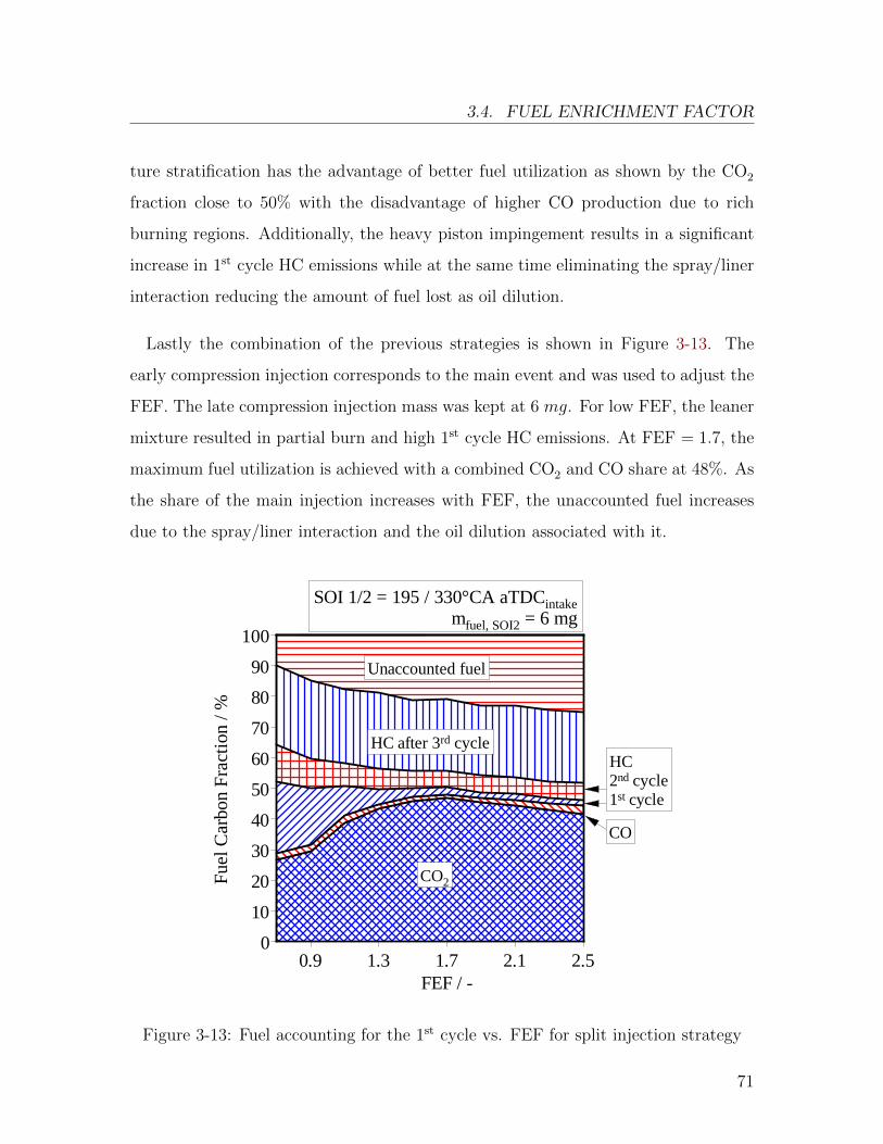
3.4. FUEL ENRICHMENT FACTOR
ture stratification has the advantage of better fuel utilization as shown by the CO2
fraction close to 50% with the disadvantage of higher CO production due to rich
burning regions. Additionally, the heavy piston impingement results in a significant
increase in 1st cycle HC emissions while at the same time eliminating the spray/liner
interaction reducing the amount of fuel lost as oil dilution.
Lastly the combination of the previous strategies is shown in Figure 3-13. The
early compression injection corresponds to the main event and was used to adjust the
FEF. The late compression injection mass was kept at 6 mg. For low FEF, the leaner
mixture resulted in partial burn and high 1st cycle HC emissions. At FEF = 1.7, the
maximum fuel utilization is achieved with a combined CO2 and CO share at 48%. As
the share of the main injection increases with FEF, the unaccounted fuel increases
due to the spray/liner interaction and the oil dilution associated with it.
Fue
l Car
bon
Fra
ctio
n /
%
0
10
20
30
40
50
60
70
80
90
100
FEF / -0.9 1.3 1.7 2.1 2.5
CO2
Unaccounted fuel
HC after 3rd cycleHC 2nd cycle1st cycle
SOI 1/2 = 195 / 330°CA aTDCintakemfuel, SOI2 = 6 mg
CO
Figure 3-13: Fuel accounting for the 1st cycle vs. FEF for split injection strategy
71
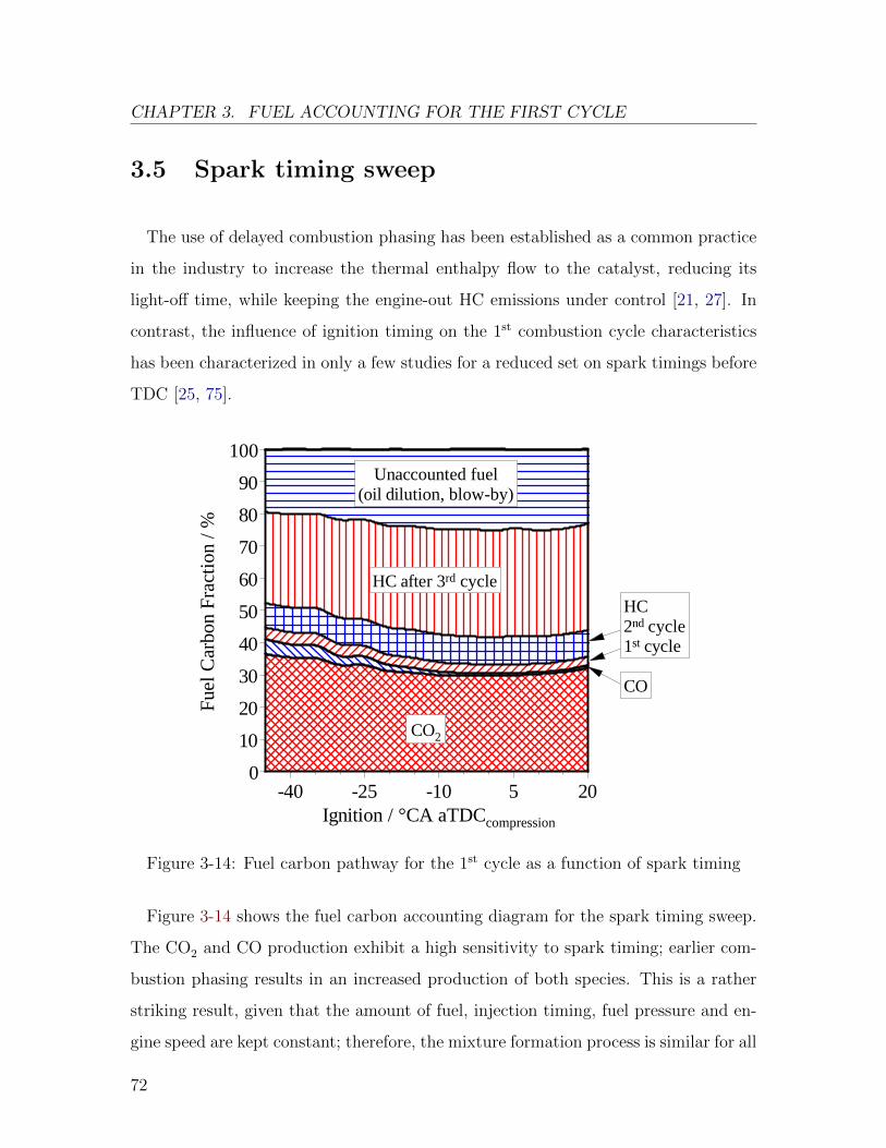
CHAPTER 3. FUEL ACCOUNTING FOR THE FIRST CYCLE
3.5 Spark timing sweep
The use of delayed combustion phasing has been established as a common practice
in the industry to increase the thermal enthalpy flow to the catalyst, reducing its
light-off time, while keeping the engine-out HC emissions under control [21, 27]. In
contrast, the influence of ignition timing on the 1st combustion cycle characteristics
has been characterized in only a few studies for a reduced set on spark timings before
TDC [25, 75].
Fue
l Car
bon
Fra
ctio
n /
%
0
10
20
30
40
50
60
70
80
90
100
Ignition / °CA aTDCcompression
-40 -25 -10 5 20
Unaccounted fuel(oil dilution, blow-by)
HC after 3rd cycle
CO2
CO
HC 2nd cycle1st cycle
Figure 3-14: Fuel carbon pathway for the 1st cycle as a function of spark timing
Figure 3-14 shows the fuel carbon accounting diagram for the spark timing sweep.
The CO2 and CO production exhibit a high sensitivity to spark timing; earlier com-
bustion phasing results in an increased production of both species. This is a rather
striking result, given that the amount of fuel, injection timing, fuel pressure and en-
gine speed are kept constant; therefore, the mixture formation process is similar for all
72
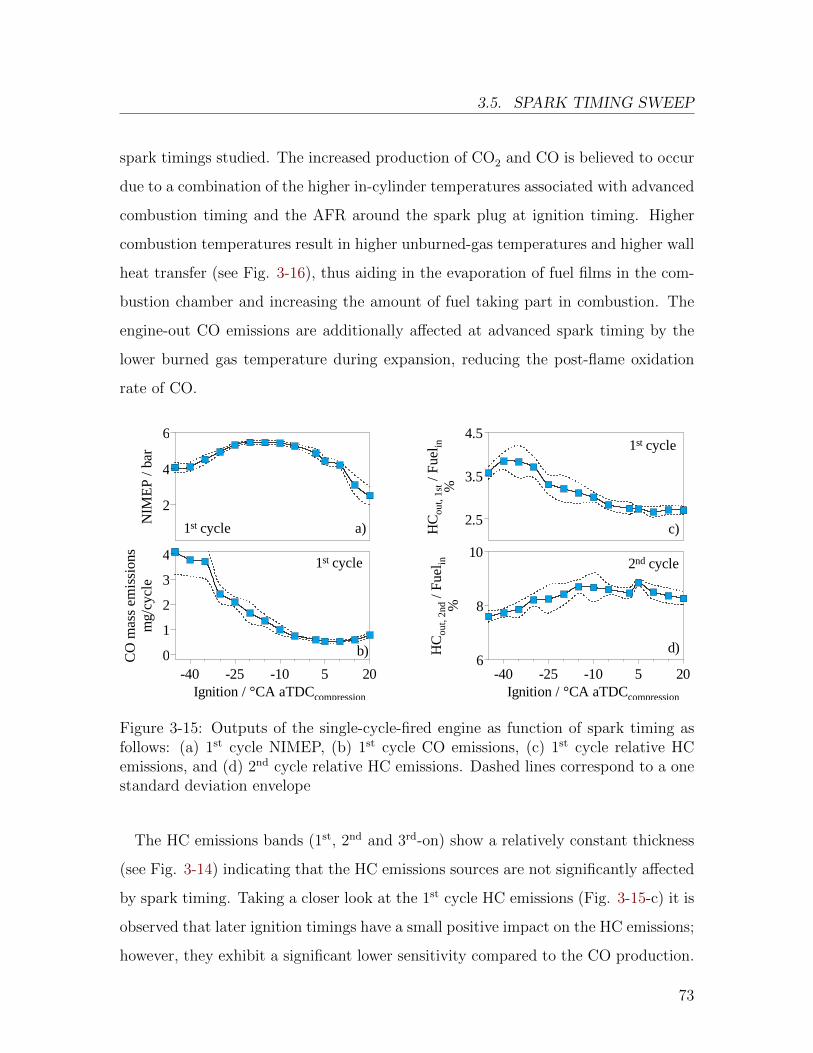
3.5. SPARK TIMING SWEEP
spark timings studied. The increased production of CO2 and CO is believed to occur
due to a combination of the higher in-cylinder temperatures associated with advanced
combustion timing and the AFR around the spark plug at ignition timing. Higher
combustion temperatures result in higher unburned-gas temperatures and higher wall
heat transfer (see Fig. 3-16), thus aiding in the evaporation of fuel films in the com-
bustion chamber and increasing the amount of fuel taking part in combustion. The
engine-out CO emissions are additionally affected at advanced spark timing by the
lower burned gas temperature during expansion, reducing the post-flame oxidation
rate of CO.
NIM
EP
/ b
ar
2
4
6
1st cycle a)
CO
ma
ss e
mis
sion
sm
g/cy
cle
0
1
2
3
4
Ignition / °CA aTDCcompression
-40 -25 -10 5 20
1st cycle
b) HC
ou
t, 2
nd /
Fue
l in%
6
8
10
Ignition / °CA aTDCcompression
-40 -25 -10 5 20
2nd cycle
d)
HC
ou
t, 1
st /
Fue
l in%
2.5
3.5
4.51st cycle
c)
Figure 3-15: Outputs of the single-cycle-fired engine as function of spark timing asfollows: (a) 1st cycle NIMEP, (b) 1st cycle CO emissions, (c) 1st cycle relative HCemissions, and (d) 2nd cycle relative HC emissions. Dashed lines correspond to a onestandard deviation envelope
The HC emissions bands (1st, 2nd and 3rd-on) show a relatively constant thickness
(see Fig. 3-14) indicating that the HC emissions sources are not significantly affected
by spark timing. Taking a closer look at the 1st cycle HC emissions (Fig. 3-15-c) it is
observed that later ignition timings have a small positive impact on the HC emissions;
however, they exhibit a significant lower sensitivity compared to the CO production.
73
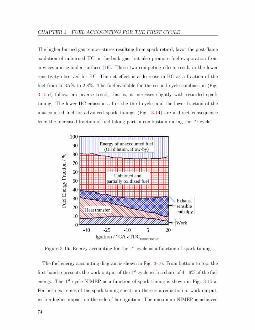
CHAPTER 3. FUEL ACCOUNTING FOR THE FIRST CYCLE
The higher burned gas temperatures resulting from spark retard, favor the post-flame
oxidation of unburned HC in the bulk gas, but also promote fuel evaporation from
crevices and cylinder surfaces [16]. These two competing effects result in the lower
sensitivity observed for HC. The net effect is a decrease in HC as a fraction of the
fuel from ≈ 3.7% to 2.8%. The fuel available for the second cycle combustion (Fig.
3-15-d) follows an inverse trend, that is, it increases slightly with retarded spark
timing. The lower HC emissions after the third cycle, and the lower fraction of the
unaccounted fuel for advanced spark timings (Fig. 3-14) are a direct consequence
from the increased fraction of fuel taking part in combustion during the 1st cycle.
Fue
l Ene
rgy
Fra
ctio
n /
%
0
10
20
30
40
50
60
70
80
90
100
Ignition / °CA aTDCcompression
-40 -25 -10 5 20
Heat transfer
Unburned andpartially oxidized fuel
Energy of unaccounted fuel(Oil dilution, Blow-by)
Exhaust sensibleenthalpy
Work
Figure 3-16: Energy accounting for the 1st cycle as a function of spark timing
The fuel energy accounting diagram is shown in Fig. 3-16. From bottom to top, the
first band represents the work output of the 1st cycle with a share of 4 - 9% of the fuel
energy. The 1st cycle NIMEP as a function of spark timing is shown in Fig. 3-15-a.
For both extremes of the spark timing spectrum there is a reduction in work output,
with a higher impact on the side of late ignition. The maximum NIMEP is achieved
74
3.6. INTAKE PRESSURE SWEEP
in a plateau region from ignition timing −25 to −5◦CA aTDCcomp.. Due to the low,
but rapidly changing, engine speed, the usual notion of proper combustion phasing
for MBT (CA50 ≈ 7◦CA aTDCcomp. and Pmax ≈ 15◦CA aTDCcomp.) does not apply
[11]. The NIMEP plateau region is a result of the competing effects between heat
transfer to the cylinder walls and the location of the maximum cylinder pressure.
As the spark timing is varied from −45 to 20◦CA aTDCcomp. the wall heat transfer
and the exhaust sensible enthalpy exhibit opposite trends. Delaying the combustion
phasing reduces the peak temperature of combustion and, consequently, the heat
transfer to the combustion chamber walls. Conversely, the lower heat transfer results
in a higher charge temperature at exhaust valve opening, thus, increasing the sensible
enthalpy of the exhausted gases. The exhaust chemical enthalpy and the fraction of
energy that cannot be accounted for mirror the results of the fuel carbon analysis.
3.6 Intake pressure sweep
Lower cylinder pressure can be beneficial for the evaporation of fuel films formed
during the injection process [46]. Furthermore, given the reduced volumetric effi-
ciency respect to the atmospheric conditions, less vaporized fuel is needed to form a
combustible mixture. The most direct way to influence the in-cylinder pressure is by
means of the manifold absolute pressure (MAP). During cranking, MAP is a function
of engine speed and throttle position. During this analysis, to isolate the effect of
MAP from that of engine speed, the throttle position was the modified parameter,
achieving a minimum MAP value of 650 mbar at a cranking speed of 280 rpm, for a
fully closed throttle valve.
The distribution of the fuel carbon as a function of MAP is shown in Fig. 3-17. The
production of CO2 increases with lower MAP values suggesting an improved mixture
75
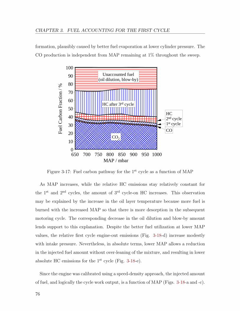
CHAPTER 3. FUEL ACCOUNTING FOR THE FIRST CYCLE
formation, plausibly caused by better fuel evaporation at lower cylinder pressure. The
CO production is independent from MAP remaining at 1% throughout the sweep.Fu
el C
arbo
n Fr
acti
on /
%
0
10
20
30
40
50
60
70
80
90
100
MAP / mbar650 700 750 800 850 900 950 1000
Unaccounted fuel(oil dilution, blow-by)
HC after 3rd cycle
CO2
CO
HC 2nd cycle1st cycle
Figure 3-17: Fuel carbon pathway for the 1st cycle as a function of MAP
As MAP increases, while the relative HC emissions stay relatively constant for
the 1st and 2nd cycles, the amount of 3rd cycle-on HC increases. This observation
may be explained by the increase in the oil layer temperature because more fuel is
burned with the increased MAP so that there is more desorption in the subsequent
motoring cycle. The corresponding decrease in the oil dilution and blow-by amount
lends support to this explanation. Despite the better fuel utilization at lower MAP
values, the relative first cycle engine-out emissions (Fig. 3-18-d) increase modestly
with intake pressure. Nevertheless, in absolute terms, lower MAP allows a reduction
in the injected fuel amount without over-leaning of the mixture, and resulting in lower
absolute HC emissions for the 1st cycle (Fig. 3-18-e).
Since the engine was calibrated using a speed-density approach, the injected amount
of fuel, and logically the cycle work output, is a function of MAP (Figs. 3-18-a and -c).
76
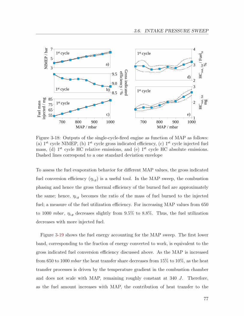
3.6. INTAKE PRESSURE SWEEP
Fuel
mas
s in
ject
ed /
mg
55657585
MAP / mbar700 800 900 1000
c)
1st cycle
NIM
EP
/ bar
3
5
7
a)
1st cycle
Gross indicated
efficiency / %
8.5
9.0
9.5
b)1st cycle
HC
out,
1st
mg
1
2
3
MAP / mbar700 800 900 1000
1st cycle
e)
HC
out,
1st /
Fue
l in%
2
3
4
d)
1st cycle
Figure 3-18: Outputs of the single-cycle-fired engine as function of MAP as follows:(a) 1st cycle NIMEP, (b) 1st cycle gross indicated efficiency, (c) 1st cycle injected fuelmass, (d) 1st cycle HC relative emissions, and (e) 1st cycle HC absolute emissions.Dashed lines correspond to a one standard deviation envelope
To assess the fuel evaporation behavior for different MAP values, the gross indicated
fuel conversion efficiency (ηi,g) is a useful tool. In the MAP sweep, the combustion
phasing and hence the gross thermal efficiency of the burned fuel are approximately
the same; hence, ηi,g becomes the ratio of the mass of fuel burned to the injected
fuel; a measure of the fuel utilization efficiency. For increasing MAP values from 650
to 1000 mbar, ηi,g decreases slightly from 9.5% to 8.8%. Thus, the fuel utilization
decreases with more injected fuel.
Figure 3-19 shows the fuel energy accounting for the MAP sweep. The first lower
band, corresponding to the fraction of energy converted to work, is equivalent to the
gross indicated fuel conversion efficiency discussed above. As the MAP is increased
from 650 to 1000 mbar the heat transfer share decreases from 15% to 10%, as the heat
transfer processes is driven by the temperature gradient in the combustion chamber
and does not scale with MAP, remaining roughly constant at 340 J . Therefore,
as the fuel amount increases with MAP, the contribution of heat transfer to the
77
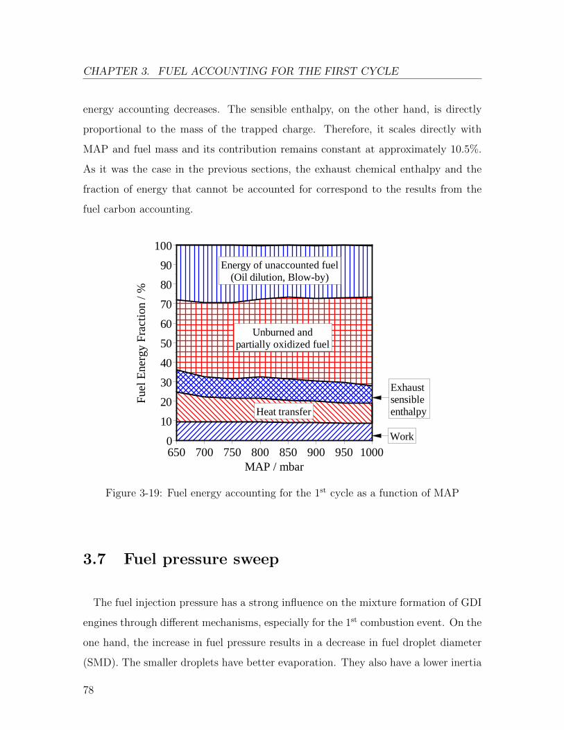
CHAPTER 3. FUEL ACCOUNTING FOR THE FIRST CYCLE
energy accounting decreases. The sensible enthalpy, on the other hand, is directly
proportional to the mass of the trapped charge. Therefore, it scales directly with
MAP and fuel mass and its contribution remains constant at approximately 10.5%.
As it was the case in the previous sections, the exhaust chemical enthalpy and the
fraction of energy that cannot be accounted for correspond to the results from the
fuel carbon accounting.
Fuel
Ene
rgy
Frac
tion
/ %
0
10
20
30
40
50
60
70
80
90
100
MAP / mbar650 700 750 800 850 900 950 1000
Heat transfer
Unburned andpartially oxidized fuel
Energy of unaccounted fuel(Oil dilution, Blow-by)
Exhaust sensibleenthalpy
Work
Figure 3-19: Fuel energy accounting for the 1st cycle as a function of MAP
3.7 Fuel pressure sweep
The fuel injection pressure has a strong influence on the mixture formation of GDI
engines through different mechanisms, especially for the 1st combustion event. On the
one hand, the increase in fuel pressure results in a decrease in fuel droplet diameter
(SMD). The smaller droplets have better evaporation. They also have a lower inertia
78
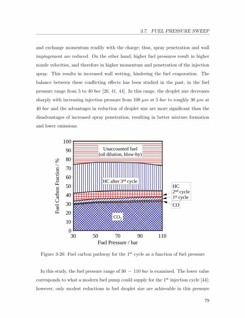
3.7. FUEL PRESSURE SWEEP
and exchange momentum readily with the charge; thus, spray penetration and wall
impingement are reduced. On the other hand, higher fuel pressures result in higher
nozzle velocities, and therefore in higher momentum and penetration of the injection
spray. This results in increased wall wetting, hindering the fuel evaporation. The
balance between these conflicting effects has been studied in the past, in the fuel
pressure range from 5 to 40 bar [20, 41, 44]. In this range, the droplet size decreases
sharply with increasing injection pressure from 100 µm at 5 bar to roughly 30 µm at
40 bar and the advantages in reduction of droplet size are more significant than the
disadvantages of increased spray penetration, resulting in better mixture formation
and lower emissions.
Fuel
Car
bon
Frac
tion
/ %
0
10
20
30
40
50
60
70
80
90
100
Fuel Pressure / bar30 50 70 90 110
Unaccounted fuel(oil dilution, blow-by)
HC after 3rd cycle
CO2
CO
HC 2nd cycle1st cycle
Figure 3-20: Fuel carbon pathway for the 1st cycle as a function of fuel pressure
In this study, the fuel pressure range of 30 − 110 bar is examined. The lower value
corresponds to what a modern fuel pump could supply for the 1st injection cycle [44];
however, only modest reductions in fuel droplet size are achievable in this pressure
79
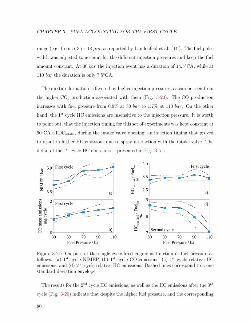
CHAPTER 3. FUEL ACCOUNTING FOR THE FIRST CYCLE
range (e.g. from ≈ 35− 18 µm, as reported by Landenfeld et al. [44]). The fuel pulse
width was adjusted to account for the different injection pressures and keep the fuel
amount constant. At 30 bar the injection event has a duration of 14.5◦CA, while at
110 bar the duration is only 7.5◦CA.
The mixture formation is favored by higher injection pressures, as can be seen from
the higher CO2 production associated with them (Fig. 3-20). The CO production
increases with fuel pressure from 0.9% at 30 bar to 1.7% at 110 bar. On the other
hand, the 1st cycle HC emissions are insensitive to the injection pressure. It is worth
to point out, that the injection timing for this set of experiments was kept constant at
90◦CA aTDCintake, during the intake valve opening; an injection timing that proved
to result in higher HC emissions due to spray interaction with the intake valve. The
detail of the 1st cycle HC emissions is presented in Fig. 3-5-c.
HC
out,
2nd
/ Fue
l in%
7
8
9
Fuel Pressure / bar30 50 70 90 110
Second cycle
d)
NIM
EP
/ bar
5.5
6.0
a)
b)
First cycle
CO
mas
s em
issi
ons
mg/
cycl
e
0
1
2
Fuel Pressure / bar30 50 70 90 110
First cycle
HC
out,
1st /
Fue
l in%
2.5
3.5
4.5First cycle
c)
Figure 3-21: Outputs of the single-cycle-fired engine as function of fuel pressure asfollows: (a) 1st cycle NIMEP, (b) 1st cycle CO emissions, (c) 1st cycle relative HCemissions, and (d) 2nd cycle relative HC emissions. Dashed lines correspond to a onestandard deviation envelope
The results for the 2nd cycle HC emissions, as well as the HC emissions after the 3rd
cycle (Fig. 3-20) indicate that despite the higher fuel pressure, and the corresponding
80
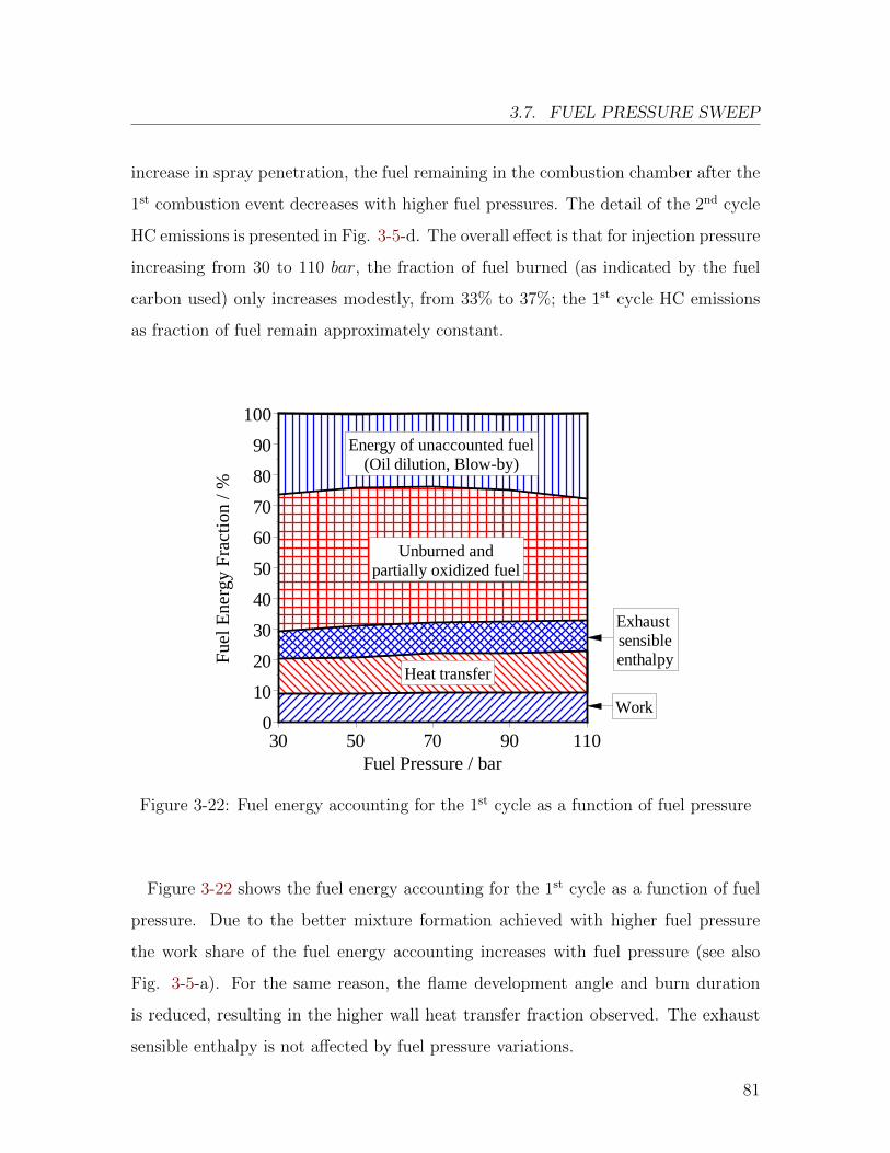
3.7. FUEL PRESSURE SWEEP
increase in spray penetration, the fuel remaining in the combustion chamber after the
1st combustion event decreases with higher fuel pressures. The detail of the 2nd cycle
HC emissions is presented in Fig. 3-5-d. The overall effect is that for injection pressure
increasing from 30 to 110 bar, the fraction of fuel burned (as indicated by the fuel
carbon used) only increases modestly, from 33% to 37%; the 1st cycle HC emissions
as fraction of fuel remain approximately constant.
Fuel
Ene
rgy
Frac
tion
/ %
0
10
20
30
40
50
60
70
80
90
100
Fuel Pressure / bar30 50 70 90 110
Heat transfer
Unburned andpartially oxidized fuel
Energy of unaccounted fuel(Oil dilution, Blow-by)
Exhaust sensibleenthalpy
Work
Figure 3-22: Fuel energy accounting for the 1st cycle as a function of fuel pressure
Figure 3-22 shows the fuel energy accounting for the 1st cycle as a function of fuel
pressure. Due to the better mixture formation achieved with higher fuel pressure
the work share of the fuel energy accounting increases with fuel pressure (see also
Fig. 3-5-a). For the same reason, the flame development angle and burn duration
is reduced, resulting in the higher wall heat transfer fraction observed. The exhaust
sensible enthalpy is not affected by fuel pressure variations.
81
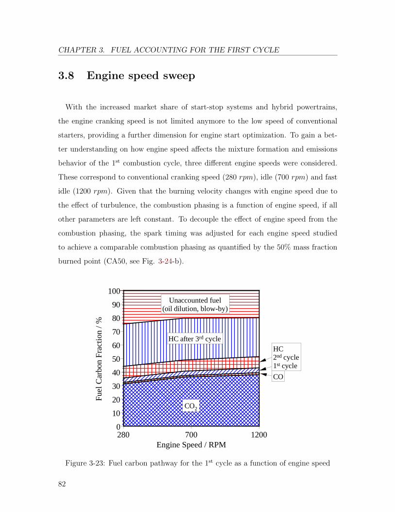
CHAPTER 3. FUEL ACCOUNTING FOR THE FIRST CYCLE
3.8 Engine speed sweep
With the increased market share of start-stop systems and hybrid powertrains,
the engine cranking speed is not limited anymore to the low speed of conventional
starters, providing a further dimension for engine start optimization. To gain a bet-
ter understanding on how engine speed affects the mixture formation and emissions
behavior of the 1st combustion cycle, three different engine speeds were considered.
These correspond to conventional cranking speed (280 rpm), idle (700 rpm) and fast
idle (1200 rpm). Given that the burning velocity changes with engine speed due to
the effect of turbulence, the combustion phasing is a function of engine speed, if all
other parameters are left constant. To decouple the effect of engine speed from the
combustion phasing, the spark timing was adjusted for each engine speed studied
to achieve a comparable combustion phasing as quantified by the 50% mass fraction
burned point (CA50, see Fig. 3-24-b).
Fuel
Car
bon
Frac
tion
/ %
0
10
20
30
40
50
60
70
80
90
100
Engine Speed / RPM280 700 1200
Unaccounted fuel(oil dilution, blow-by)
HC after 3rd cycle
CO2
CO
HC 2nd cycle1st cycle
Figure 3-23: Fuel carbon pathway for the 1st cycle as a function of engine speed
82
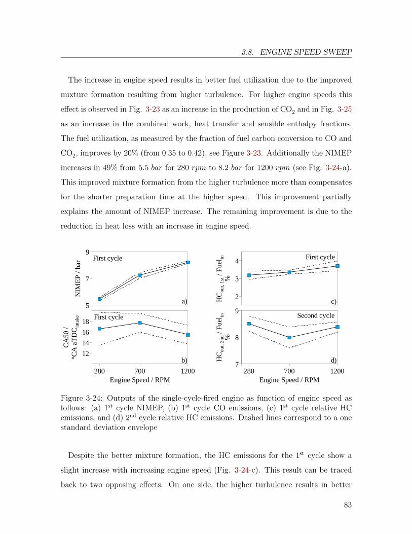
3.8. ENGINE SPEED SWEEP
The increase in engine speed results in better fuel utilization due to the improved
mixture formation resulting from higher turbulence. For higher engine speeds this
effect is observed in Fig. 3-23 as an increase in the production of CO2 and in Fig. 3-25
as an increase in the combined work, heat transfer and sensible enthalpy fractions.
The fuel utilization, as measured by the fraction of fuel carbon conversion to CO and
CO2, improves by 20% (from 0.35 to 0.42), see Figure 3-23. Additionally the NIMEP
increases in 49% from 5.5 bar for 280 rpm to 8.2 bar for 1200 rpm (see Fig. 3-24-a).
This improved mixture formation from the higher turbulence more than compensates
for the shorter preparation time at the higher speed. This improvement partially
explains the amount of NIMEP increase. The remaining improvement is due to the
reduction in heat loss with an increase in engine speed.H
Co
ut,
2n
d / F
uel in
%
7
8
9
Engine Speed / RPM280 700 1200
d)
Second cycle
NIM
EP
/ b
ar
5
7
9First cycle
a)
CA
50 /
°CA
aT
DC i
nta
ke
12
14
16
18
Engine Speed / RPM280 700 1200
First cycle
b)
HC
ou
t, 1
st /
Fue
l in%
2
3
4First cycle
c)
Figure 3-24: Outputs of the single-cycle-fired engine as function of engine speed asfollows: (a) 1st cycle NIMEP, (b) 1st cycle CO emissions, (c) 1st cycle relative HCemissions, and (d) 2nd cycle relative HC emissions. Dashed lines correspond to a onestandard deviation envelope
Despite the better mixture formation, the HC emissions for the 1st cycle show a
slight increase with increasing engine speed (Fig. 3-24-c). This result can be traced
back to two opposing effects. On one side, the higher turbulence results in better
83
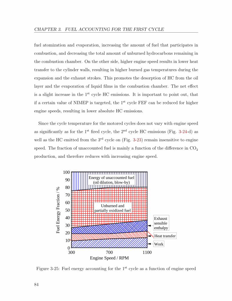
CHAPTER 3. FUEL ACCOUNTING FOR THE FIRST CYCLE
fuel atomization and evaporation, increasing the amount of fuel that participates in
combustion, and decreasing the total amount of unburned hydrocarbons remaining in
the combustion chamber. On the other side, higher engine speed results in lower heat
transfer to the cylinder walls, resulting in higher burned gas temperatures during the
expansion and the exhaust strokes. This promotes the desorption of HC from the oil
layer and the evaporation of liquid films in the combustion chamber. The net effect
is a slight increase in the 1st cycle HC emissions. It is important to point out, that
if a certain value of NIMEP is targeted, the 1st cycle FEF can be reduced for higher
engine speeds, resulting in lower absolute HC emissions.
Since the cycle temperature for the motored cycles does not vary with engine speed
as significantly as for the 1st fired cycle, the 2nd cycle HC emissions (Fig. 3-24-d) as
well as the HC emitted from the 3rd cycle on (Fig. 3-23) remain insensitive to engine
speed. The fraction of unaccounted fuel is mainly a function of the difference in CO2
production, and therefore reduces with increasing engine speed.
Fuel
Ene
rgy
Frac
tion
/ %
0
10
20
30
40
50
60
70
80
90
100
Engine Speed / RPM300 700 1100
Unburned andpartially oxidized fuel
Energy of unaccounted fuel(oil dilution, blow-by)
Exhaust sensibleenthalpy
Work
Heat transfer
Figure 3-25: Fuel energy accounting for the 1st cycle as a function of engine speed
84
3.9. FINDINGS
3.9 Findings
Using a fuel carbon accounting analysis for the 1st combustion cycle, the study pre-
sented in this paper aims to quantify the amount of fuel participating in combustion
as well as the amount of unburned HC left after combustion leading to HC emissions
and residual fuel in the combustion chamber. A one-variable-at-a-time approach was
used to isolate the effects of the different parameters affecting the 1st combustion cy-
cle. The study focused in the effects of fuel enrichment, injection and ignition timing,
intake manifold and fuel pressure, and engine speed, with the following key findings:
� The injection timing determines the type and degree of interaction between
the injection spray and the elements of the combustion chamber. For this par-
ticular configuration, it was found that injection during the early compression
stroke results in lower HC emissions, due to reduced interaction with the intake
valve and piston crown. Injection events close to BDC result in increased liner
wetting, therefore increasing the amount of fuel lost as oil dilution.
� The 1st cycle fuel enrichment affects on a one-to-one proportion the absolute
1st cycle HC emissions. Thus, reducing the fuel enrichment is beneficial for HC
emissions reduction, but increases the probability of a partial burn or a mis-
fire, which would result in unacceptably high HC emissions. Despite the fuel
conversion efficiency being constant at 30% for all FEFs, the energy distribu-
tion changes significantly. For low FEF, the late combustion phasing causes
increased charge temperatures at EVO and lower temperatures during combus-
tion. As a result the exhaust sensible enthalpy is larger while the wall heat
transfer is reduced.
� The spark timing, and the associated combustion phasing, impacts both the
amount of fuel participating in combustion as well as the rate of post-flame
oxidation. As a general trend, later spark timing results in reduced CO and
85
CHAPTER 3. FUEL ACCOUNTING FOR THE FIRST CYCLE
slightly lower HC emissions at the cost of lower work output. As already men-
tioned in the previous point, late combustion phasing affects directly the charge
temperatures at exhaust valve opening and the maximum temperature during
combustion. Consequently, the exhaust sensible enthalpy and the wall heat
transfer follow inverse trends and are highly sensitive to spark timing.
� A reduced intake manifold pressure has a positive influence in mixture prepa-
ration, resulting in more fuel participating in combustion. The relative HC
emissions are not sensitive to MAP. Due to the reduced amount of fuel injected
(at constant enrichment factor), the absolute HC emissions are lower at the cost
of lower work output.
� The decrease in droplet size from higher injection pressures is offset by the
increase in fuel spray penetration. Fuel utilization increases with injection pres-
sure. The relative HC emissions, however, are not sensitive to injection pressure.
� Higher engine speed promotes turbulence. The improvement in turbulent mass
transfer more than compensates for the reduction in mixture preparation time;
hence, fuel utilization improves with engine speed. The relative HC emissions
increase modestly with higher engine speeds. At the same combustion phasing,
NIMEP increases with engine speed because of the better fuel utilization and
of the heat loss reduction. For a targeted NIMEP value, therefore, less fuel is
needed at the higher engine speed, resulting in reduction of the absolute HC
emissions.
86
Chapter 4
Cycle-by-cycle analysis of cold
crank-start
This chapter seeks to expand the understanding of the CO, HC, NOx, and PM/PN
emissions behavior during the cold crank-start process of a GDI engine. For that
purpose the initial 3 engine cycles are analyzed individually under a set of parameters
that include among others the mass of injected fuel, the start of injection (SOI), and
the ignition timing. The focus is on the dependence of the CO, HC, PM/PN and
NOx emissions. Additionally, the interactions between cycles are also considered by
studying the impact that the heat transfer history and the residual fuel from previous
injection events have on the mixture formation and FEF requirement.
The PM/PN emissions per cycle decrease by more than an order of magnitude as
the crank-start progresses from the 1st to the 3rd cycle, while the HC emissions stay
relatively constant. The wall heat transfer during the previous cycles, as controlled
by the combustion phasing, has a more significant influence on the mixture formation
process for the current cycle than the amount of residual fuel. The results show that
the rise in HC emissions caused by the injection spray interacting with the intake
87
CHAPTER 4. CYCLE-BY-CYCLE ANALYSIS OF COLD CRANK-START
valves and piston crown is reduced as the cranking process progresses. Combustion
phasing retard significantly reduces the PM emission. The HC emissions, however, are
relatively not sensitive to combustion phasing in the range of interest. NOx emissions
mirror the maximum cylinder temperature when mixture stratification is not present.
Part of the results presented in this chapter have been published in the SAE Inter-
national Journal of Engines [60, 62].
4.1 Experiments description
In order to quantify the pollutant mass emissions of the individual engine cycles
during crank-start the sampling probes of the fast response analyzers were located as
close as possible to the exhaust valve. The methodology for converting concentration
measurements to mass emissions is found in Section 2.2.2. The focus of this study
was placed on cylinder #4. To suppress pressure, temperature and composition inter-
actions from neighboring cylinders, the engine was operated in single-cylinder mode.
As a consequence, the engine was unable to achieve a speed transient that is repre-
sentative of a 4-cylinder engine during crank-start. To circumvent this, the engine
was torque-assisted by a 10 hp electric motor during the simulated crank-start ex-
periments. The motor triggering point and speed-ramp were tuned to achieve similar
speed traces between multi-cylinder and single-cylinder crank-start. Each experiment
starts with the engine motoring at cranking speed until steady state conditions are
achieved. After the steady-state motoring, and depending on the engine cycle of
interest, 1, 2 or 3 combustion events take place in cylinder #4 (see Fig. 4-1 a-c).
Thereafter, engine is motored while the exhaust flow composition and temperatures
are recorded until the purging of residual HC is completed and the steady-state con-
ditions are attained. Five experiments were run for each experimental condition; the
average values are reported.
88
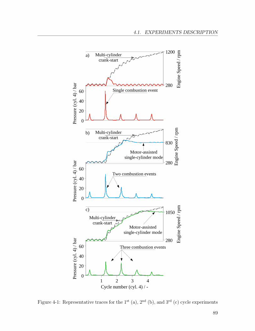
4.1. EXPERIMENTS DESCRIPTION
Eng
ine
Spee
d / r
pm
280
1200Multi-cylinder
crank-starta)
Pres
sure
(cy
l. 4)
/ ba
r
0
20
40
60 Single combustion event
Eng
ine
Spee
d / r
pm
280
830
Multi-cylindercrank-start
b)
Motor-assistedsingle-cylinder mode
Pres
sure
(cy
l. 4)
/ ba
r
0
20
40
60Two combustion events
Eng
ine
Spee
d / r
pm
280
1050Multi-cylinder
crank-start
c)
Motor-assistedsingle-cylinder mode
Pres
sure
(cy
l. 4)
/ ba
r
0
20
40
60
Cycle number (cyl. 4) / -1 2 3 4
Three combustion events
Figure 4-1: Representative traces for the 1st (a), 2nd (b), and 3rd (c) cycle experiments
89
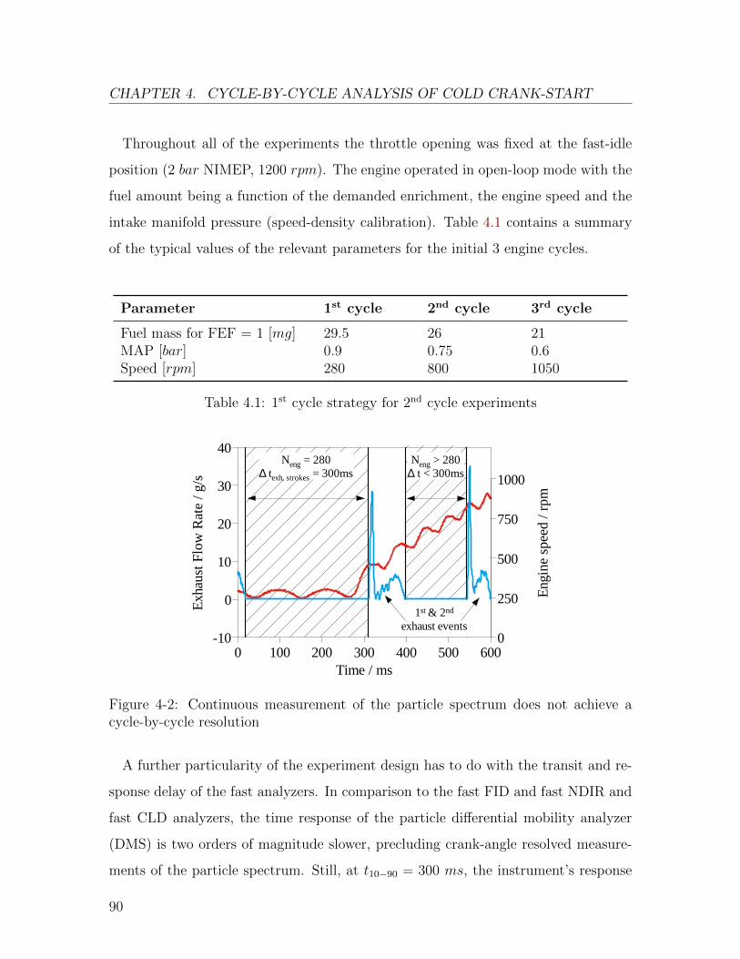
CHAPTER 4. CYCLE-BY-CYCLE ANALYSIS OF COLD CRANK-START
Throughout all of the experiments the throttle opening was fixed at the fast-idle
position (2 bar NIMEP, 1200 rpm). The engine operated in open-loop mode with the
fuel amount being a function of the demanded enrichment, the engine speed and the
intake manifold pressure (speed-density calibration). Table 4.1 contains a summary
of the typical values of the relevant parameters for the initial 3 engine cycles.
Parameter 1st cycle 2nd cycle 3rd cycle
Fuel mass for FEF = 1 [mg] 29.5 26 21MAP [bar] 0.9 0.75 0.6Speed [rpm] 280 800 1050
Table 4.1: 1st cycle strategy for 2nd cycle experiments
Eng
ine
spee
d / r
pm
0
250
500
750
1000
1st & 2nd
exhaust events
Neng = 280∆ texh. strokes = 300ms
Neng > 280∆ t < 300ms
Exh
aust
Flo
w R
ate
/ g/s
-10
0
10
20
30
40
Time / ms0 100 200 300 400 500 600
Figure 4-2: Continuous measurement of the particle spectrum does not achieve acycle-by-cycle resolution
A further particularity of the experiment design has to do with the transit and re-
sponse delay of the fast analyzers. In comparison to the fast FID and fast NDIR and
fast CLD analyzers, the time response of the particle differential mobility analyzer
(DMS) is two orders of magnitude slower, precluding crank-angle resolved measure-
ments of the particle spectrum. Still, at t10−90 = 300 ms, the instrument’s response
90
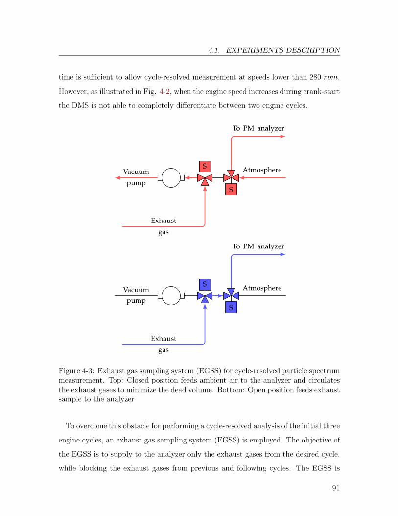
4.1. EXPERIMENTS DESCRIPTION
time is sufficient to allow cycle-resolved measurement at speeds lower than 280 rpm.
However, as illustrated in Fig. 4-2, when the engine speed increases during crank-start
the DMS is not able to completely differentiate between two engine cycles.
To PM analyzer
AtmosphereVacuum
pump
Exhaust
gas
S
S
To PM analyzer
AtmosphereVacuumpump
Exhaust
gas
S
S
Figure 4-3: Exhaust gas sampling system (EGSS) for cycle-resolved particle spectrummeasurement. Top: Closed position feeds ambient air to the analyzer and circulatesthe exhaust gases to minimize the dead volume. Bottom: Open position feeds exhaustsample to the analyzer
To overcome this obstacle for performing a cycle-resolved analysis of the initial three
engine cycles, an exhaust gas sampling system (EGSS) is employed. The objective of
the EGSS is to supply to the analyzer only the exhaust gases from the desired cycle,
while blocking the exhaust gases from previous and following cycles. The EGSS is
91
CHAPTER 4. CYCLE-BY-CYCLE ANALYSIS OF COLD CRANK-START
located upstream of the DMS and consists of two three-way solenoid valves connected
in series. In the “closed” position (Fig. 4-3-top), the exhaust gas is circulated around
the system by a rotary vane vacuum pump in order to minimize dead volumes, while
the DMS is allowed to sample ambient air in order to maintain its internal pressure
within range. In the “open” position (Fig. 4-3-bottom) the exhaust and sample flows
are connected, and the DMS is able to carry out defectively the particle spectrum
measurement for the desired engine cycle. The solenoid valves have a 3/32” orifice
and an opening time of 10 ms. The EGSS is controlled by a programmable micro-
controller that uses the crankshaft encoder signal as an input for the timely actuation
of the solenoid valves.
4.2 First cycle analysis
A number of variables influence the mixture formation process and the emissions
behavior of the 1st firing cycle during the cranking process. This section focuses on
the four most relevant injection parameters using a one-variable-at-a-time approach.
The variables studied are: Start of injection (SOI), fuel enrichment factor (FEF),
ignition timing, and fuel pressure. The swept ranges and the nominal points are
presented in Table 4.2. Unless otherwise stated, all the variables stay constant at the
nominal values during the different sweeps.
Parameter Sweep range Nominal value
SOI [◦CA aTDCintake] 30 − 315 ∆ = 15 90FEF [−] 1.7 − 3.5 ∆ = 0.2 2.5Spark [◦CA aTDCcomp.] −45 − 20 ∆ = 5 -10Fuel pressure [bar] 30 − 110 ∆ = 20 50
Table 4.2: Experimental scope for the 1st cycle emissions
92
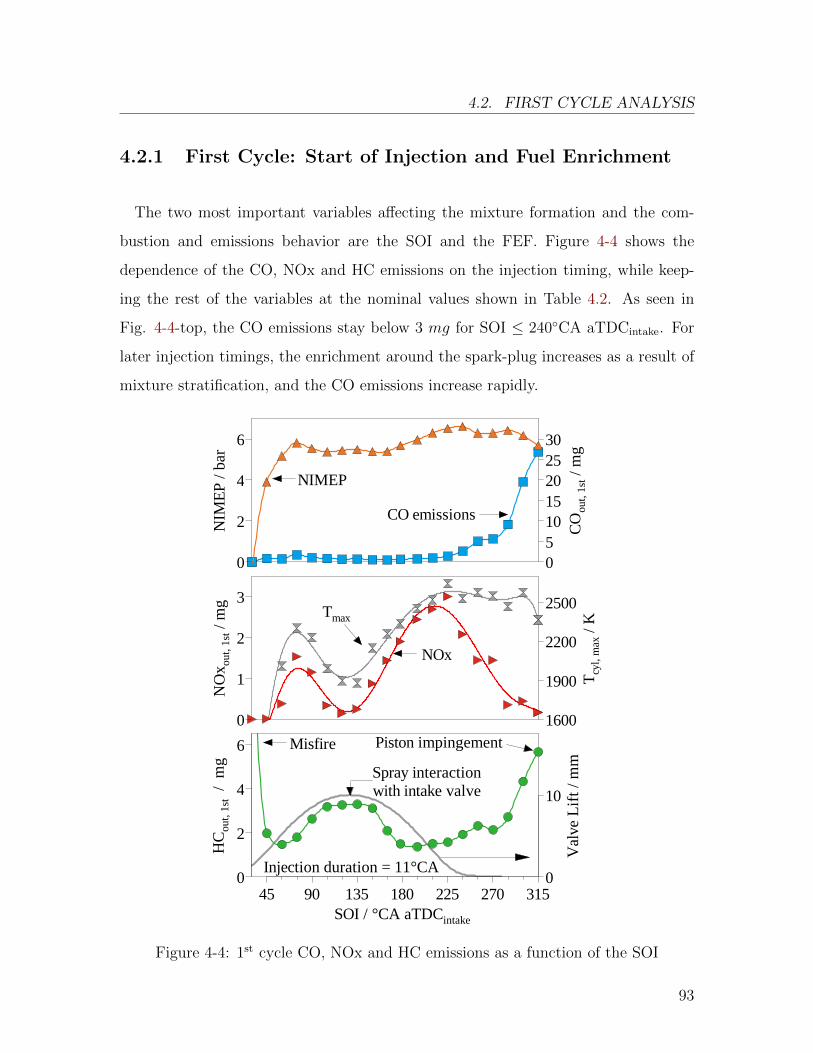
4.2. FIRST CYCLE ANALYSIS
4.2.1 First Cycle: Start of Injection and Fuel Enrichment
The two most important variables affecting the mixture formation and the com-
bustion and emissions behavior are the SOI and the FEF. Figure 4-4 shows the
dependence of the CO, NOx and HC emissions on the injection timing, while keep-
ing the rest of the variables at the nominal values shown in Table 4.2. As seen in
Fig. 4-4-top, the CO emissions stay below 3 mg for SOI ≤ 240◦CA aTDCintake. For
later injection timings, the enrichment around the spark-plug increases as a result of
mixture stratification, and the CO emissions increase rapidly.
Val
ve L
ift /
mm
0
10
Injection duration = 11°CA
HC
out,
1st
/ m
g
0
2
4
6
SOI / °CA aTDCintake
45 90 135 180 225 270 315
Piston impingement
Spray interactionwith intake valve
Misfire
CO
out,
1st
/ mg
051015202530
NIM
EP
/ ba
r
0
2
4
6
CO emissions
NIMEP
Tcy
l, m
ax /
K
1600
1900
2200
2500
NO
x out
, 1st
/ mg
0
1
2
3
NOx
Tmax
Figure 4-4: 1st cycle CO, NOx and HC emissions as a function of the SOI
93
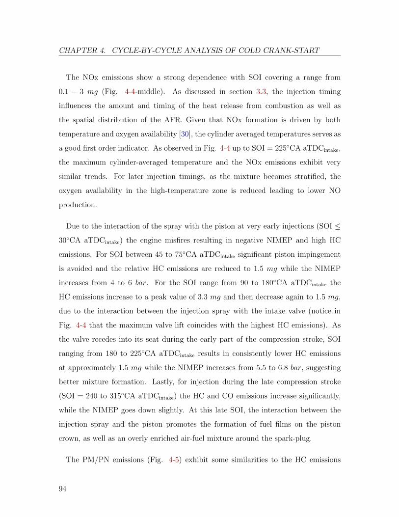
CHAPTER 4. CYCLE-BY-CYCLE ANALYSIS OF COLD CRANK-START
The NOx emissions show a strong dependence with SOI covering a range from
0.1 − 3 mg (Fig. 4-4-middle). As discussed in section 3.3, the injection timing
influences the amount and timing of the heat release from combustion as well as
the spatial distribution of the AFR. Given that NOx formation is driven by both
temperature and oxygen availability [30], the cylinder averaged temperatures serves as
a good first order indicator. As observed in Fig. 4-4 up to SOI = 225◦CA aTDCintake,
the maximum cylinder-averaged temperature and the NOx emissions exhibit very
similar trends. For later injection timings, as the mixture becomes stratified, the
oxygen availability in the high-temperature zone is reduced leading to lower NO
production.
Due to the interaction of the spray with the piston at very early injections (SOI ≤
30◦CA aTDCintake) the engine misfires resulting in negative NIMEP and high HC
emissions. For SOI between 45 to 75◦CA aTDCintake significant piston impingement
is avoided and the relative HC emissions are reduced to 1.5 mg while the NIMEP
increases from 4 to 6 bar. For the SOI range from 90 to 180◦CA aTDCintake the
HC emissions increase to a peak value of 3.3 mg and then decrease again to 1.5 mg,
due to the interaction between the injection spray with the intake valve (notice in
Fig. 4-4 that the maximum valve lift coincides with the highest HC emissions). As
the valve recedes into its seat during the early part of the compression stroke, SOI
ranging from 180 to 225◦CA aTDCintake results in consistently lower HC emissions
at approximately 1.5 mg while the NIMEP increases from 5.5 to 6.8 bar, suggesting
better mixture formation. Lastly, for injection during the late compression stroke
(SOI = 240 to 315◦CA aTDCintake) the HC and CO emissions increase significantly,
while the NIMEP goes down slightly. At this late SOI, the interaction between the
injection spray and the piston promotes the formation of fuel films on the piston
crown, as well as an overly enriched air-fuel mixture around the spark-plug.
The PM/PN emissions (Fig. 4-5) exhibit some similarities to the HC emissions
94
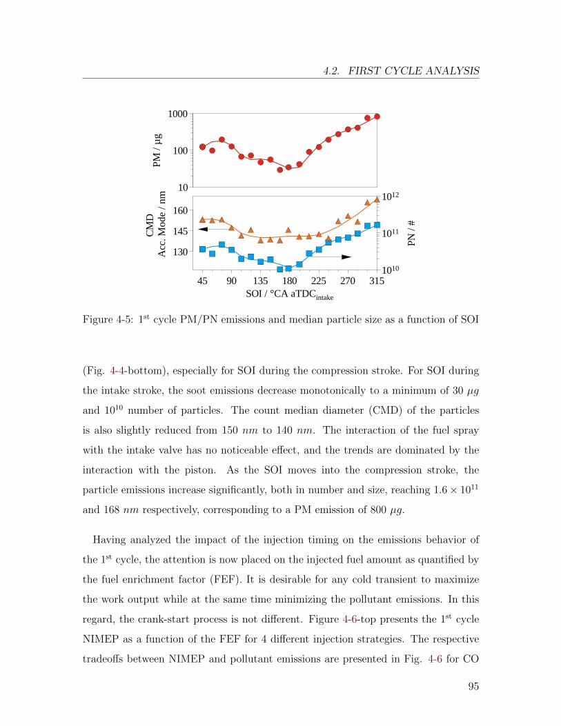
4.2. FIRST CYCLE ANALYSIS
PM
/ µ
g
10
100
1000
PN
/ #
1010
1011
1012
SOI / °CA aTDCintake
45 90 135 180 225 270 315
CM
D
Acc
. Mod
e /
nm
130
145
160
Figure 4-5: 1st cycle PM/PN emissions and median particle size as a function of SOI
(Fig. 4-4-bottom), especially for SOI during the compression stroke. For SOI during
the intake stroke, the soot emissions decrease monotonically to a minimum of 30 µg
and 1010 number of particles. The count median diameter (CMD) of the particles
is also slightly reduced from 150 nm to 140 nm. The interaction of the fuel spray
with the intake valve has no noticeable effect, and the trends are dominated by the
interaction with the piston. As the SOI moves into the compression stroke, the
particle emissions increase significantly, both in number and size, reaching 1.6× 10¹¹
and 168 nm respectively, corresponding to a PM emission of 800 µg.
Having analyzed the impact of the injection timing on the emissions behavior of
the 1st cycle, the attention is now placed on the injected fuel amount as quantified by
the fuel enrichment factor (FEF). It is desirable for any cold transient to maximize
the work output while at the same time minimizing the pollutant emissions. In this
regard, the crank-start process is not different. Figure 4-6-top presents the 1st cycle
NIMEP as a function of the FEF for 4 different injection strategies. The respective
tradeoffs between NIMEP and pollutant emissions are presented in Fig. 4-6 for CO
95
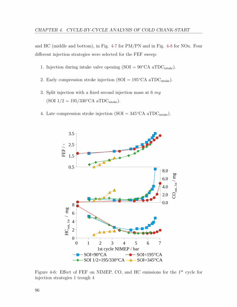
CHAPTER 4. CYCLE-BY-CYCLE ANALYSIS OF COLD CRANK-START
and HC (middle and bottom), in Fig. 4-7 for PM/PN and in Fig. 4-8 for NOx. Four
different injection strategies were selected for the FEF sweep:
1. Injection during intake valve opening (SOI = 90◦CA aTDCintake).
2. Early compression stroke injection (SOI = 195◦CA aTDCintake).
3. Split injection with a fixed second injection mass at 6 mg
(SOI 1/2 = 195/330◦CA aTDCintake).
4. Late compression stroke injection (SOI = 345◦CA aTDCintake).
FE
F /
-
0.5
1.5
2.5
3.5
HC
out,
1st
/ m
g
0
2
4
6
8
1st cycle NIMEP / bar0 1 2 3 4 5 6 7
SOI=90°CA SOI=195°CA SOI 1/2=195/330°CA SOI=345°CA
CO
out,
1st
/ mg
0.0
2.0
4.0
6.0
8.0
Figure 4-6: Effect of FEF on NIMEP, CO, and HC emissions for the 1st cycle forinjection strategies 1 trough 4
96
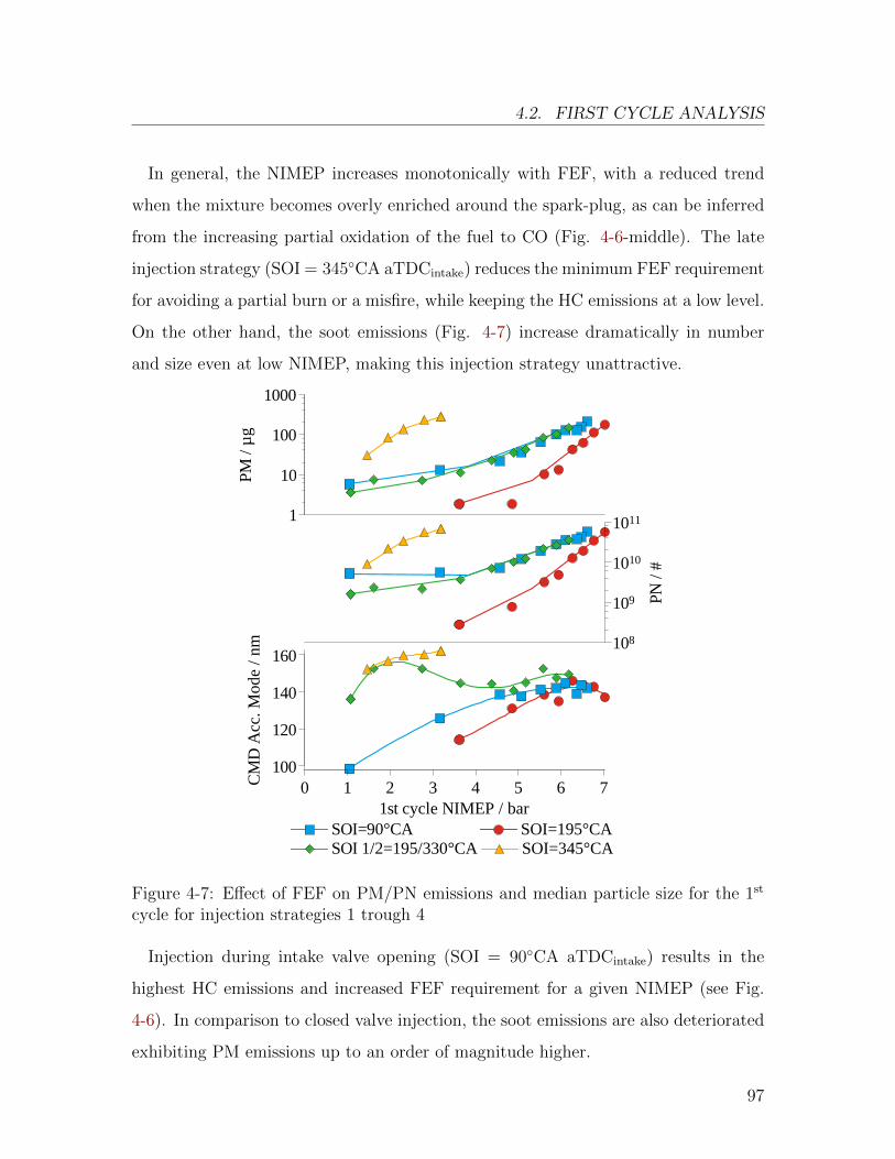
4.2. FIRST CYCLE ANALYSIS
In general, the NIMEP increases monotonically with FEF, with a reduced trend
when the mixture becomes overly enriched around the spark-plug, as can be inferred
from the increasing partial oxidation of the fuel to CO (Fig. 4-6-middle). The late
injection strategy (SOI = 345◦CA aTDCintake) reduces the minimum FEF requirement
for avoiding a partial burn or a misfire, while keeping the HC emissions at a low level.
On the other hand, the soot emissions (Fig. 4-7) increase dramatically in number
and size even at low NIMEP, making this injection strategy unattractive.
PM
/ µ
g
1
10
100
1000
CM
D A
cc. M
ode
/ n
m
100
120
140
160
1st cycle NIMEP / bar0 1 2 3 4 5 6 7
SOI=90°CA SOI=195°CA SOI 1/2=195/330°CA SOI=345°CA
PN
/ #
108
109
1010
1011
Figure 4-7: Effect of FEF on PM/PN emissions and median particle size for the 1st
cycle for injection strategies 1 trough 4
Injection during intake valve opening (SOI = 90◦CA aTDCintake) results in the
highest HC emissions and increased FEF requirement for a given NIMEP (see Fig.
4-6). In comparison to closed valve injection, the soot emissions are also deteriorated
exhibiting PM emissions up to an order of magnitude higher.
97
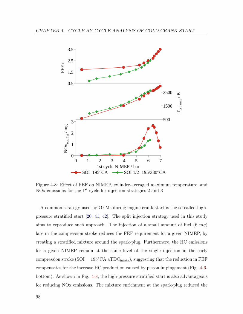
CHAPTER 4. CYCLE-BY-CYCLE ANALYSIS OF COLD CRANK-START
NO
x out
, 1st
/ mg
0
1
2
3
1st cycle NIMEP / bar0 1 2 3 4 5 6 7
SOI=195°CA SOI 1/2=195/330°CAT
cyl,
max
/ K
500
1500
2500
FE
F /
-
0.5
1.5
2.5
3.5
Figure 4-8: Effect of FEF on NIMEP, cylinder-averaged maximum temperature, andNOx emissions for the 1st cycle for injection strategies 2 and 3
A common strategy used by OEMs during engine crank-start is the so called high-
pressure stratified start [20, 41, 42]. The split injection strategy used in this study
aims to reproduce such approach. The injection of a small amount of fuel (6 mg)
late in the compression stroke reduces the FEF requirement for a given NIMEP, by
creating a stratified mixture around the spark-plug. Furthermore, the HC emissions
for a given NIMEP remain at the same level of the single injection in the early
compression stroke (SOI = 195◦CA aTDCintake), suggesting that the reduction in FEF
compensates for the increase HC production caused by piston impingement (Fig. 4-6-
bottom). As shown in Fig. 4-8, the high-pressure stratified start is also advantageous
for reducing NOx emissions. The mixture enrichment at the spark-plug reduced the
98
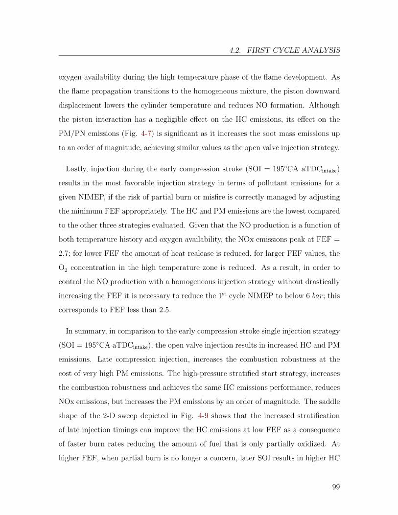
4.2. FIRST CYCLE ANALYSIS
oxygen availability during the high temperature phase of the flame development. As
the flame propagation transitions to the homogeneous mixture, the piston downward
displacement lowers the cylinder temperature and reduces NO formation. Although
the piston interaction has a negligible effect on the HC emissions, its effect on the
PM/PN emissions (Fig. 4-7) is significant as it increases the soot mass emissions up
to an order of magnitude, achieving similar values as the open valve injection strategy.
Lastly, injection during the early compression stroke (SOI = 195◦CA aTDCintake)
results in the most favorable injection strategy in terms of pollutant emissions for a
given NIMEP, if the risk of partial burn or misfire is correctly managed by adjusting
the minimum FEF appropriately. The HC and PM emissions are the lowest compared
to the other three strategies evaluated. Given that the NO production is a function of
both temperature history and oxygen availability, the NOx emissions peak at FEF =
2.7; for lower FEF the amount of heat realease is reduced, for larger FEF values, the
O2 concentration in the high temperature zone is reduced. As a result, in order to
control the NO production with a homogeneous injection strategy without drastically
increasing the FEF it is necessary to reduce the 1st cycle NIMEP to below 6 bar; this
corresponds to FEF less than 2.5.
In summary, in comparison to the early compression stroke single injection strategy
(SOI = 195◦CA aTDCintake), the open valve injection results in increased HC and PM
emissions. Late compression injection, increases the combustion robustness at the
cost of very high PM emissions. The high-pressure stratified start strategy, increases
the combustion robustness and achieves the same HC emissions performance, reduces
NOx emissions, but increases the PM emissions by an order of magnitude. The saddle
shape of the 2-D sweep depicted in Fig. 4-9 shows that the increased stratification
of late injection timings can improve the HC emissions at low FEF as a consequence
of faster burn rates reducing the amount of fuel that is only partially oxidized. At
higher FEF, when partial burn is no longer a concern, later SOI results in higher HC
99
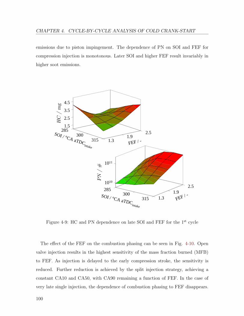
CHAPTER 4. CYCLE-BY-CYCLE ANALYSIS OF COLD CRANK-START
emissions due to piston impingement. The dependence of PN on SOI and FEF for
compression injection is monotonous. Later SOI and higher FEF result invariably in
higher soot emissions.
285300
315SOI / °CA aTDC
intake
1.31.9
2.5
FEF / -
1.5
2.5
3.5
4.5
HC
/ m
g
285300
315SOI / °CA aTDC
intake
1.31.9
2.5
FEF / -
1010
1011
PN /
#
Figure 4-9: HC and PN dependence on late SOI and FEF for the 1st cycle
The effect of the FEF on the combustion phasing can be seen in Fig. 4-10. Open
valve injection results in the highest sensitivity of the mass fraction burned (MFB)
to FEF. As injection is delayed to the early compression stroke, the sensitivity is
reduced. Further reduction is achieved by the split injection strategy, achieving a
constant CA10 and CA50, with CA90 remaining a function of FEF. In the case of
very late single injection, the dependence of combustion phasing to FEF disappears.
100
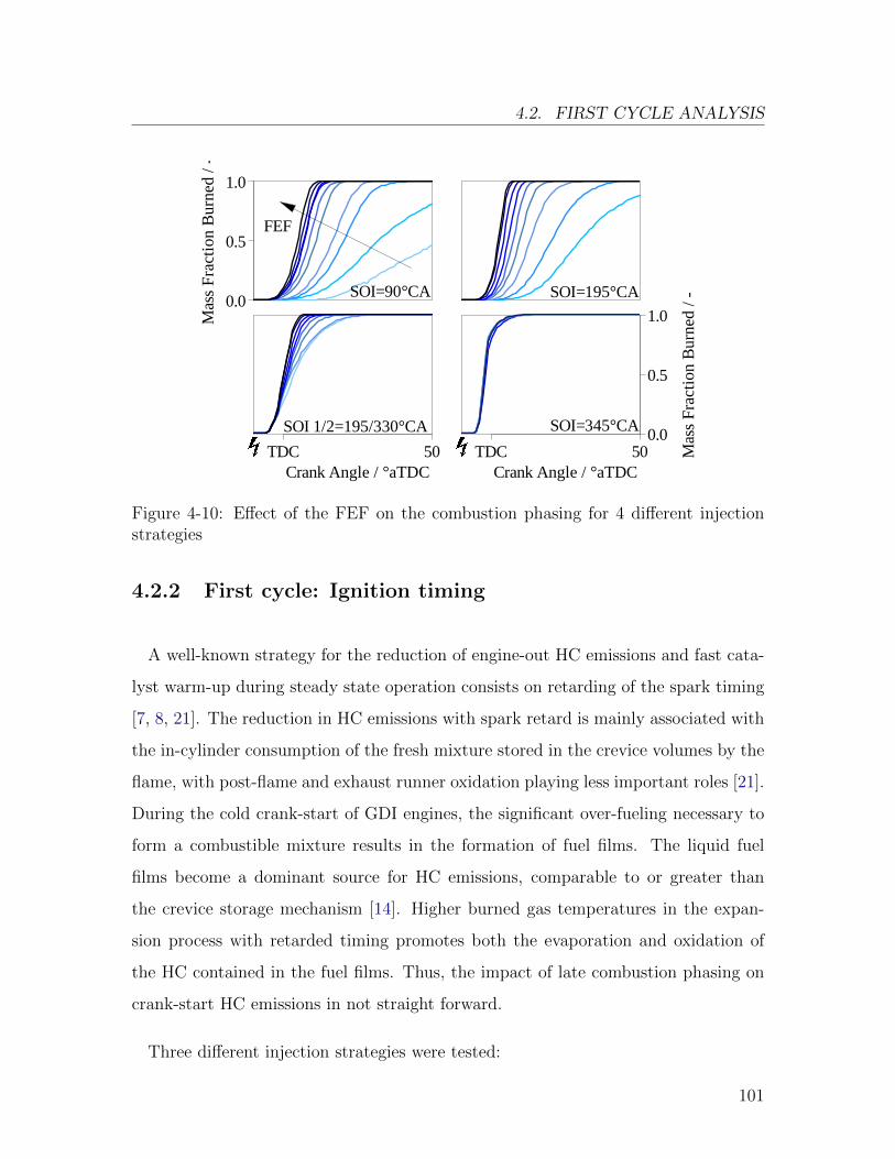
4.2. FIRST CYCLE ANALYSIS
Crank Angle / °aTDCTDC 50
SOI 1/2=195/330°CA
Mas
s F
ract
ion
Bur
ned
/ -
0.0
0.5
1.0
SOI=90°CA SOI=195°CA
FEF
Mas
s F
ract
ion
Bur
ned
/ -
0.0
0.5
1.0
Crank Angle / °aTDCTDC 50
SOI=345°CA
Figure 4-10: Effect of the FEF on the combustion phasing for 4 different injectionstrategies
4.2.2 First cycle: Ignition timing
A well-known strategy for the reduction of engine-out HC emissions and fast cata-
lyst warm-up during steady state operation consists on retarding of the spark timing
[7, 8, 21]. The reduction in HC emissions with spark retard is mainly associated with
the in-cylinder consumption of the fresh mixture stored in the crevice volumes by the
flame, with post-flame and exhaust runner oxidation playing less important roles [21].
During the cold crank-start of GDI engines, the significant over-fueling necessary to
form a combustible mixture results in the formation of fuel films. The liquid fuel
films become a dominant source for HC emissions, comparable to or greater than
the crevice storage mechanism [14]. Higher burned gas temperatures in the expan-
sion process with retarded timing promotes both the evaporation and oxidation of
the HC contained in the fuel films. Thus, the impact of late combustion phasing on
crank-start HC emissions in not straight forward.
Three different injection strategies were tested:
101
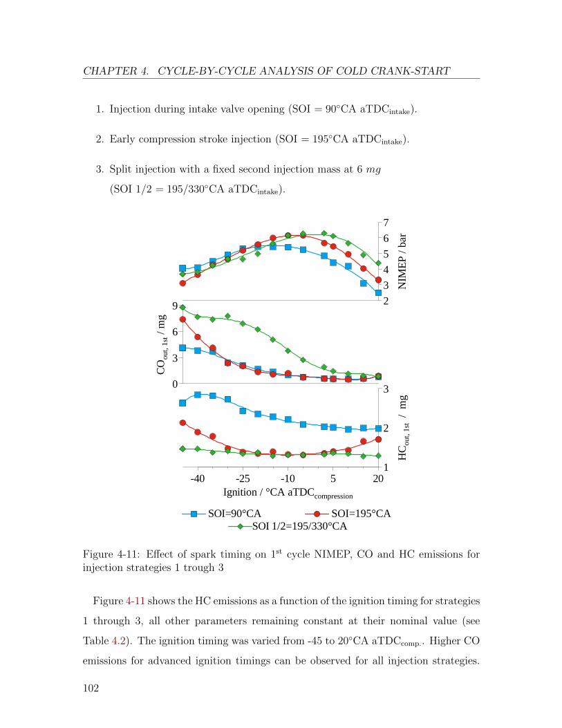
CHAPTER 4. CYCLE-BY-CYCLE ANALYSIS OF COLD CRANK-START
1. Injection during intake valve opening (SOI = 90◦CA aTDCintake).
2. Early compression stroke injection (SOI = 195◦CA aTDCintake).
3. Split injection with a fixed second injection mass at 6 mg
(SOI 1/2 = 195/330◦CA aTDCintake).
SOI=90°CA SOI=195°CA SOI 1/2=195/330°CA
NIM
EP
/ b
ar
2
3
4
5
6
7
HC
out,
1st
/ m
g
1
2
3
Ignition / °CA aTDCcompression
-40 -25 -10 5 20
CO
out,
1st
/ mg
0
3
6
9
Figure 4-11: Effect of spark timing on 1st cycle NIMEP, CO and HC emissions forinjection strategies 1 trough 3
Figure 4-11 shows the HC emissions as a function of the ignition timing for strategies
1 through 3, all other parameters remaining constant at their nominal value (see
Table 4.2). The ignition timing was varied from -45 to 20◦CA aTDCcomp.. Higher CO
emissions for advanced ignition timings can be observed for all injection strategies.
102
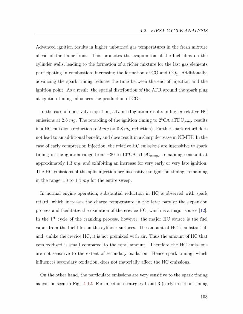
4.2. FIRST CYCLE ANALYSIS
Advanced ignition results in higher unburned gas temperatures in the fresh mixture
ahead of the flame front. This promotes the evaporation of the fuel films on the
cylinder walls, leading to the formation of a richer mixture for the last gas elements
participating in combustion, increasing the formation of CO and CO2. Additionally,
advancing the spark timing reduces the time between the end of injection and the
ignition point. As a result, the spatial distribution of the AFR around the spark plug
at ignition timing influences the production of CO.
In the case of open valve injection, advanced ignition results in higher relative HC
emissions at 2.8 mg. The retarding of the ignition timing to 2◦CA aTDCcomp. results
in a HC emissions reduction to 2 mg (≈ 0.8 mg reduction). Further spark retard does
not lead to an additional benefit, and does result in a sharp decrease in NIMEP. In the
case of early compression injection, the relative HC emissions are insensitive to spark
timing in the ignition range from −30 to 10◦CA aTDCcomp., remaining constant at
approximately 1.3 mg, and exhibiting an increase for very early or very late ignition.
The HC emissions of the split injection are insensitive to ignition timing, remaining
in the range 1.3 to 1.4 mg for the entire sweep.
In normal engine operation, substantial reduction in HC is observed with spark
retard, which increases the charge temperature in the later part of the expansion
process and facilitates the oxidation of the crevice HC, which is a major source [12].
In the 1st cycle of the cranking process, however, the major HC source is the fuel
vapor from the fuel film on the cylinder surfaces. The amount of HC is substantial,
and, unlike the crevice HC, it is not premixed with air. Thus the amount of HC that
gets oxidized is small compared to the total amount. Therefore the HC emissions
are not sensitive to the extent of secondary oxidation. Hence spark timing, which
influences secondary oxidation, does not materially affect the HC emissions.
On the other hand, the particulate emissions are very sensitive to the spark timing
as can be seen in Fig. 4-12. For injection strategies 1 and 3 (early injection timing
103
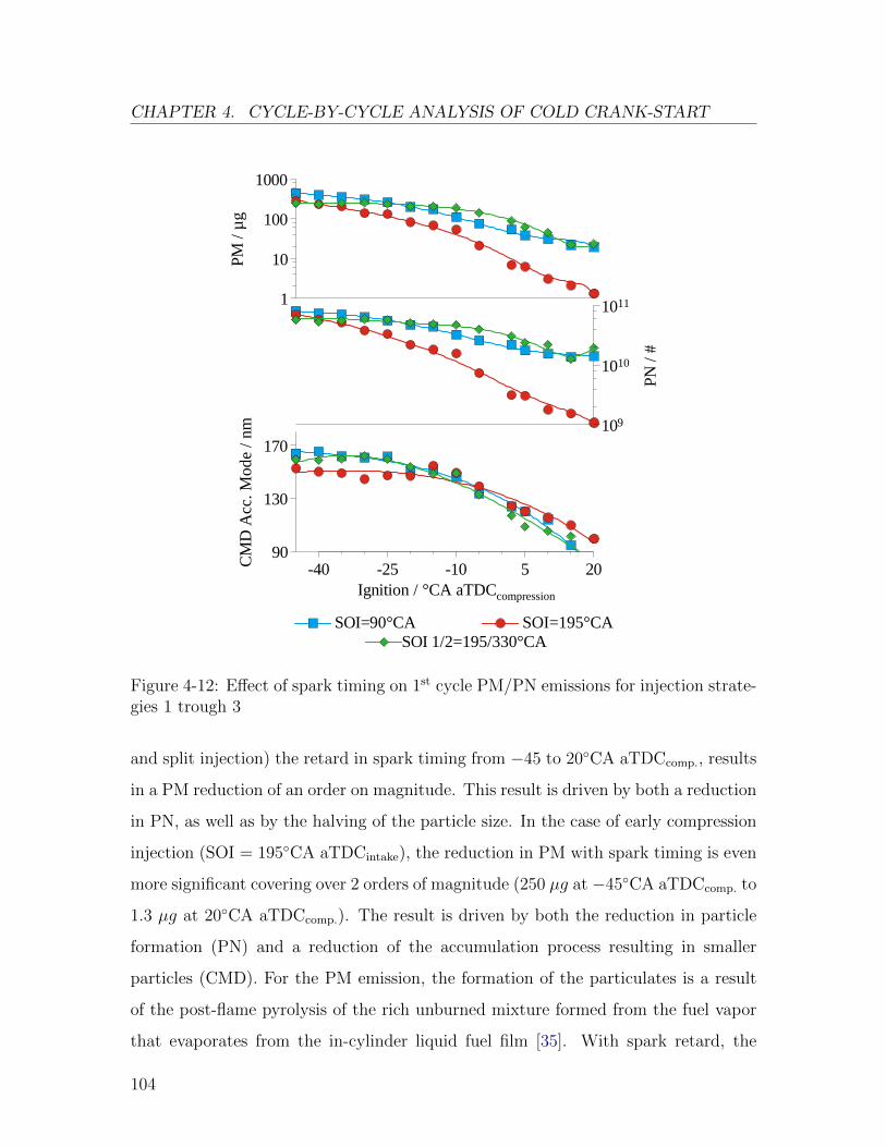
CHAPTER 4. CYCLE-BY-CYCLE ANALYSIS OF COLD CRANK-START
SOI=90°CA SOI=195°CA SOI 1/2=195/330°CA
PM
/ µ
g
1
10
100
1000
CM
D A
cc. M
ode
/ n
m
90
130
170
Ignition / °CA aTDCcompression
-40 -25 -10 5 20
PN
/ #
109
1010
1011
Figure 4-12: Effect of spark timing on 1st cycle PM/PN emissions for injection strate-gies 1 trough 3
and split injection) the retard in spark timing from −45 to 20◦CA aTDCcomp., results
in a PM reduction of an order on magnitude. This result is driven by both a reduction
in PN, as well as by the halving of the particle size. In the case of early compression
injection (SOI = 195◦CA aTDCintake), the reduction in PM with spark timing is even
more significant covering over 2 orders of magnitude (250 µg at −45◦CA aTDCcomp. to
1.3 µg at 20◦CA aTDCcomp.). The result is driven by both the reduction in particle
formation (PN) and a reduction of the accumulation process resulting in smaller
particles (CMD). For the PM emission, the formation of the particulates is a result
of the post-flame pyrolysis of the rich unburned mixture formed from the fuel vapor
that evaporates from the in-cylinder liquid fuel film [35]. With spark retard, the
104
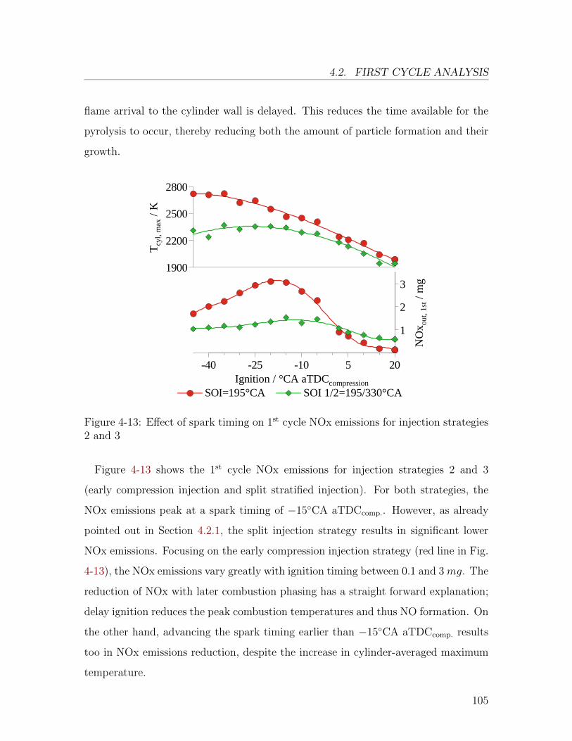
4.2. FIRST CYCLE ANALYSIS
flame arrival to the cylinder wall is delayed. This reduces the time available for the
pyrolysis to occur, thereby reducing both the amount of particle formation and their
growth.
SOI=195°CA SOI 1/2=195/330°CA
NO
x out
, 1st
/ mg
1
2
3
Ignition / °CA aTDCcompression
-40 -25 -10 5 20
Tcy
l, m
ax /
K
1900
2200
2500
2800
Figure 4-13: Effect of spark timing on 1st cycle NOx emissions for injection strategies2 and 3
Figure 4-13 shows the 1st cycle NOx emissions for injection strategies 2 and 3
(early compression injection and split stratified injection). For both strategies, the
NOx emissions peak at a spark timing of −15◦CA aTDCcomp.. However, as already
pointed out in Section 4.2.1, the split injection strategy results in significant lower
NOx emissions. Focusing on the early compression injection strategy (red line in Fig.
4-13), the NOx emissions vary greatly with ignition timing between 0.1 and 3 mg. The
reduction of NOx with later combustion phasing has a straight forward explanation;
delay ignition reduces the peak combustion temperatures and thus NO formation. On
the other hand, advancing the spark timing earlier than −15◦CA aTDCcomp. results
too in NOx emissions reduction, despite the increase in cylinder-averaged maximum
temperature.
105
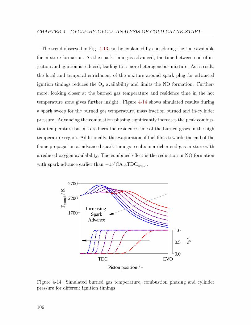
CHAPTER 4. CYCLE-BY-CYCLE ANALYSIS OF COLD CRANK-START
The trend observed in Fig. 4-13 can be explained by considering the time available
for mixture formation. As the spark timing is advanced, the time between end of in-
jection and ignition is reduced, leading to a more heterogeneous mixture. As a result,
the local and temporal enrichment of the mxiture around spark plug for advanced
ignition timings reduces the O2 availability and limits the NO formation. Further-
more, looking closer at the burned gas temperature and residence time in the hot
temperature zone gives further insight. Figure 4-14 shows simulated results during
a spark sweep for the burned gas temperature, mass fraction burned and in-cylinder
pressure. Advancing the combustion phasing significantly increases the peak combus-
tion temperature but also reduces the residence time of the burned gases in the high
temperature region. Additionally, the evaporation of fuel films towards the end of the
flame propagation at advanced spark timings results in a richer end-gas mixture with
a reduced oxygen availability. The combined effect is the reduction in NO formation
with spark advance earlier than −15◦CA aTDCcomp..
Piston position / -
TDC EVO
T
burn
ed /
K
1700
2200
2700
Increasing Spark
Advance
xb
/ -
0.0
0.5
1.0
Figure 4-14: Simulated burned gas temperature, combustion phasing and cylinderpressure for different ignition timings
106
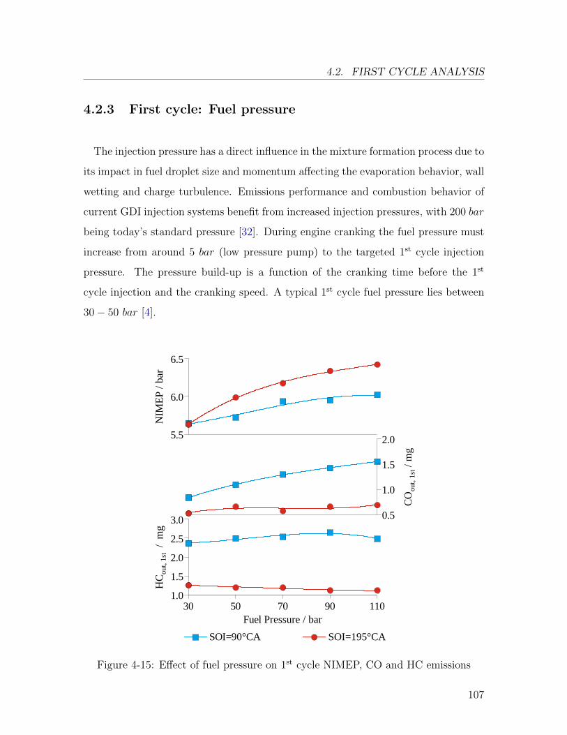
4.2. FIRST CYCLE ANALYSIS
4.2.3 First cycle: Fuel pressure
The injection pressure has a direct influence in the mixture formation process due to
its impact in fuel droplet size and momentum affecting the evaporation behavior, wall
wetting and charge turbulence. Emissions performance and combustion behavior of
current GDI injection systems benefit from increased injection pressures, with 200 bar
being today’s standard pressure [32]. During engine cranking the fuel pressure must
increase from around 5 bar (low pressure pump) to the targeted 1st cycle injection
pressure. The pressure build-up is a function of the cranking time before the 1st
cycle injection and the cranking speed. A typical 1st cycle fuel pressure lies between
30− 50 bar [4].
SOI=90°CA SOI=195°CA
NIM
EP
/ b
ar
5.5
6.0
6.5
CO
out,
1st
/ mg
0.5
1.0
1.5
2.0
HC
out,
1st
/ m
g
1.0
1.5
2.0
2.5
3.0
Fuel Pressure / bar30 50 70 90 110
Figure 4-15: Effect of fuel pressure on 1st cycle NIMEP, CO and HC emissions
107
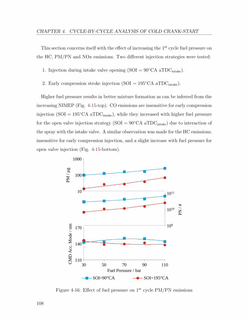
CHAPTER 4. CYCLE-BY-CYCLE ANALYSIS OF COLD CRANK-START
This section concerns itself with the effect of increasing the 1st cycle fuel pressure on
the HC, PM/PN and NOx emissions. Two different injection strategies were tested:
1. Injection during intake valve opening (SOI = 90◦CA aTDCintake).
2. Early compression stroke injection (SOI = 195◦CA aTDCintake).
Higher fuel pressure results in better mixture formation as can be inferred from the
increasing NIMEP (Fig. 4-15-top). CO emissions are insensitive for early compression
injection (SOI = 195◦CA aTDCintake), while they increased with higher fuel pressure
for the open valve injection strategy (SOI = 90◦CA aTDCintake) due to interaction of
the spray with the intake valve. A similar observation was made for the HC emissions;
insensitive for early compression injection, and a slight increase with fuel pressure for
open valve injection (Fig. 4-15-bottom).
PM
/ µ
g
10
100
1000
CM
D A
cc. M
ode
/ n
m
110
140
170
Fuel Pressure / bar30 50 70 90 110
SOI=90°CA SOI=195°CA
PN
/ #
109
1010
1011
Figure 4-16: Effect of fuel pressure on 1st cycle PM/PN emissions
108
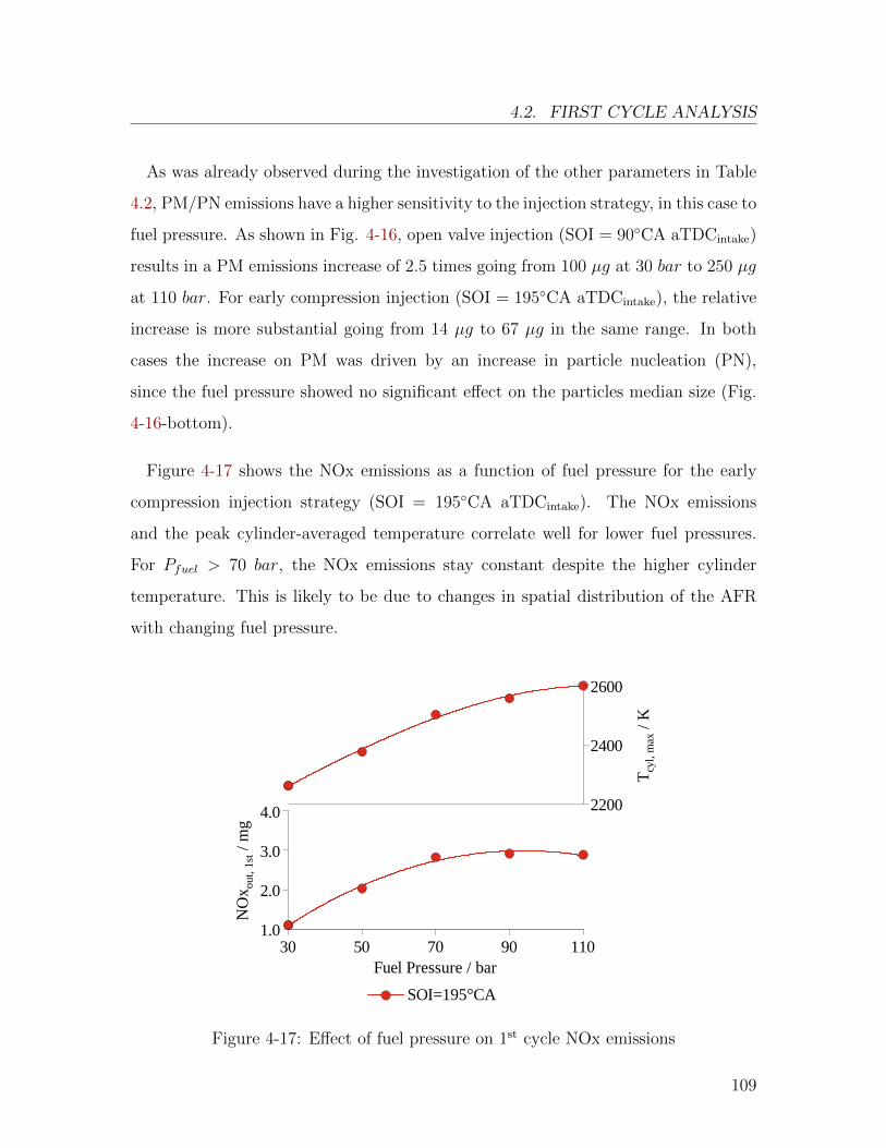
4.2. FIRST CYCLE ANALYSIS
As was already observed during the investigation of the other parameters in Table
4.2, PM/PN emissions have a higher sensitivity to the injection strategy, in this case to
fuel pressure. As shown in Fig. 4-16, open valve injection (SOI = 90◦CA aTDCintake)
results in a PM emissions increase of 2.5 times going from 100 µg at 30 bar to 250 µg
at 110 bar. For early compression injection (SOI = 195◦CA aTDCintake), the relative
increase is more substantial going from 14 µg to 67 µg in the same range. In both
cases the increase on PM was driven by an increase in particle nucleation (PN),
since the fuel pressure showed no significant effect on the particles median size (Fig.
4-16-bottom).
Figure 4-17 shows the NOx emissions as a function of fuel pressure for the early
compression injection strategy (SOI = 195◦CA aTDCintake). The NOx emissions
and the peak cylinder-averaged temperature correlate well for lower fuel pressures.
For Pfuel > 70 bar, the NOx emissions stay constant despite the higher cylinder
temperature. This is likely to be due to changes in spatial distribution of the AFR
with changing fuel pressure.T
cyl,
max
/ K
2200
2400
2600
NO
x out
, 1st
/ mg
1.0
2.0
3.0
4.0
Fuel Pressure / bar30 50 70 90 110
SOI=195°CA
Figure 4-17: Effect of fuel pressure on 1st cycle NOx emissions
109
CHAPTER 4. CYCLE-BY-CYCLE ANALYSIS OF COLD CRANK-START
In summary, increasing the 1st cycle fuel pressure from the levels found in today’s
GDI engines has only a reduced benefit on the 1st cycle NIMEP, which is more than
offset by the worse performance in PM/PN emissions. The HC emissions behavior
was linked to the SOI, with increased HC emissions for injection during IVO at higher
fuel pressures; and insensitive behavior for early compression stroke SOI. Although
reducing the fuel pressures below 50 bar improves the emissions performance, it is
not recommended since it would pose a constraint for late SOI strategies.
4.3 Second cycle analysis
The 2nd engine cycle during crank-start differs significantly from the 1st cycle pre-
viously described in the main following points:
� Presence of residual fuel from previous injection event.
� Wall heating from previous combustion event.
� Presence of residual exhaust gases during the mixture formation.
� Higher engine speed and lower manifold pressure.
This section focuses on the three of the most relevant injection parameters using a
one-variable-at-a-time approach. The variables studied are: Start of injection (SOI),
fuel enrichment factor (FEF), and ignition timing. The swept ranges can be found
in Table 4.3. In order to decouple the effects of the 1st cycle injection strategy on
the 2nd cycle emission analysis, the 1st cycle strategy was kept constant as shown in
Table 4.4.
Lastly, the interactions between the 1st and 2nd cycles are also studied by considering
the impact that the heat transfer history and the residual fuel from the previous
110
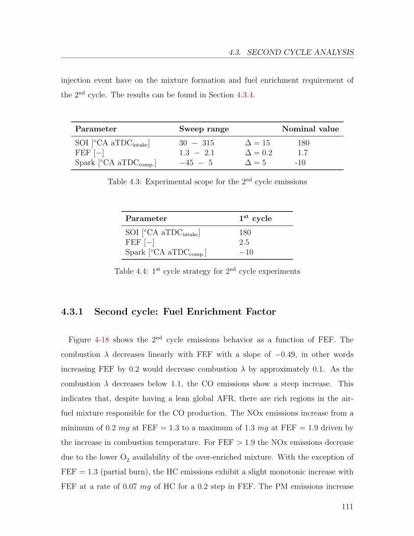
4.3. SECOND CYCLE ANALYSIS
injection event have on the mixture formation and fuel enrichment requirement of
the 2nd cycle. The results can be found in Section 4.3.4.
Parameter Sweep range Nominal value
SOI [◦CA aTDCintake] 30 − 315 ∆ = 15 180FEF [−] 1.3 − 2.1 ∆ = 0.2 1.7Spark [◦CA aTDCcomp.] −45 − 5 ∆ = 5 -10
Table 4.3: Experimental scope for the 2nd cycle emissions
Parameter 1st cycle
SOI [◦CA aTDCintake] 180FEF [−] 2.5Spark [◦CA aTDCcomp.] −10
Table 4.4: 1st cycle strategy for 2nd cycle experiments
4.3.1 Second cycle: Fuel Enrichment Factor
Figure 4-18 shows the 2nd cycle emissions behavior as a function of FEF. The
combustion λ decreases linearly with FEF with a slope of −0.49, in other words
increasing FEF by 0.2 would decrease combustion λ by approximately 0.1. As the
combustion λ decreases below 1.1, the CO emissions show a steep increase. This
indicates that, despite having a lean global AFR, there are rich regions in the air-
fuel mixture responsible for the CO production. The NOx emissions increase from a
minimum of 0.2 mg at FEF = 1.3 to a maximum of 1.3 mg at FEF = 1.9 driven by
the increase in combustion temperature. For FEF > 1.9 the NOx emissions decrease
due to the lower O2 availability of the over-enriched mixture. With the exception of
FEF = 1.3 (partial burn), the HC emissions exhibit a slight monotonic increase with
FEF at a rate of 0.07 mg of HC for a 0.2 step in FEF. The PM emissions increase
111
CHAPTER 4. CYCLE-BY-CYCLE ANALYSIS OF COLD CRANK-START
is more substantial with FEF, for a 0.2 step in FEF, the 2nd cycle PM emissions
increase in ≈ 2.5 µg. A fuel enrichment factor of 1.7 provides a good balance between
emissions behavior and the combustion robustness.
FEF 2nd cycle / -1.3 1.5 1.7 1.9 2.1
HC
2nd
/ m
g
0.5
1.0
1.5
2.0
CO
2nd /
mg
0.3
0.7
1.1
1.5
PM
2nd /
µg
1
3
5
7
9
Com
b. λ
/ -
1.01.11.21.31.41.5
Tcy
l, m
ax /
K
1400
1900
2400
2900
NO
x 2n
d / m
g
0.2
0.7
1.2
Figure 4-18: 2nd cycle CO, NOx, HC and PM emissions as a function of FEF
4.3.2 Second cycle: Start of injection
Following a similar approach as in Section 4.2.1, the analysis is extended to the
2nd cycle dependence on the injection timing. The FEF and spark timing were held
constant at 1.7 and −10◦CA aTDCcomp. throughout the sweep as well as the injection
strategy of the 1st cycle. The FEF selection for the 2nd cycle is based on the trends
presented in Section 4.3.1 and resulted in a fuel mass of approximately 44 mg and an
injection duration of 15◦CA.
112
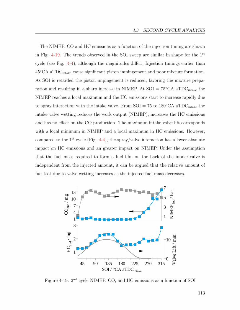
4.3. SECOND CYCLE ANALYSIS
The NIMEP, CO and HC emissions as a function of the injection timing are shown
in Fig. 4-19. The trends observed in the SOI sweep are similar in shape for the 1st
cycle (see Fig. 4-4), although the magnitudes differ. Injection timings earlier than
45◦CA aTDCintake cause significant piston impingement and poor mixture formation.
As SOI is retarded the piston impingement is reduced, favoring the mixture prepa-
ration and resulting in a sharp increase in NIMEP. At SOI = 75◦CA aTDCintake the
NIMEP reaches a local maximum and the HC emissions start to increase rapidly due
to spray interaction with the intake valve. From SOI = 75 to 180◦CA aTDCintake the
intake valve wetting reduces the work output (NIMEP), increases the HC emissions
and has no effect on the CO production. The maximum intake valve lift corresponds
with a local minimum in NIMEP and a local maximum in HC emissions. However,
compared to the 1st cycle (Fig. 4-4), the spray/valve interaction has a lower absolute
impact on HC emissions and an greater impact on NIMEP. Under the assumption
that the fuel mass required to form a fuel film on the back of the intake valve is
independent from the injected amount, it can be argued that the relative amount of
fuel lost due to valve wetting increases as the injected fuel mass decreases.N
IME
P2n
d / b
ar
1
3
5
7
HC
2nd /
mg
1
2
3
SOI / °CA aTDCintake
45 90 135 180 225 270 315
CO
2nd /
mg
1
4
7
10
13
Val
ve L
ift /
mm
0
10
Figure 4-19: 2nd cycle NIMEP, CO, and HC emissions as a function of SOI
113
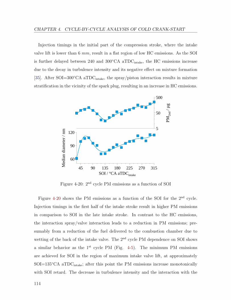
CHAPTER 4. CYCLE-BY-CYCLE ANALYSIS OF COLD CRANK-START
Injection timings in the initial part of the compression stroke, where the intake
valve lift is lower than 6 mm, result in a flat region of low HC emissions. As the SOI
is further delayed between 240 and 300◦CA aTDCintake, the HC emissions increase
due to the decay in turbulence intensity and its negative effect on mixture formation
[35]. After SOI=300◦CA aTDCintake, the spray/piston interaction results in mixture
stratification in the vicinity of the spark plug, resulting in an increase in HC emissions.
Med
ian
dia
me
ter
/ nm
60
90
120
SOI / °CA aTDCintake
45 90 135 180 225 270 315P
M2n
d / µ
g
5
50
500
Figure 4-20: 2nd cycle PM emissions as a function of SOI
Figure 4-20 shows the PM emissions as a function of the SOI for the 2nd cycle.
Injection timings in the first half of the intake stroke result in higher PM emissions
in comparison to SOI in the late intake stroke. In contrast to the HC emissions,
the interaction spray/valve interaction leads to a reduction in PM emissions; pre-
sumably from a reduction of the fuel delivered to the combustion chamber due to
wetting of the back of the intake valve. The 2nd cycle PM dependence on SOI shows
a similar behavior as the 1st cycle PM (Fig. 4-5). The minimum PM emissions
are achieved for SOI in the region of maximum intake valve lift, at approximately
SOI=135◦CA aTDCintake; after this point the PM emissions increase monotonically
with SOI retard. The decrease in turbulence intensity and the interaction with the
114
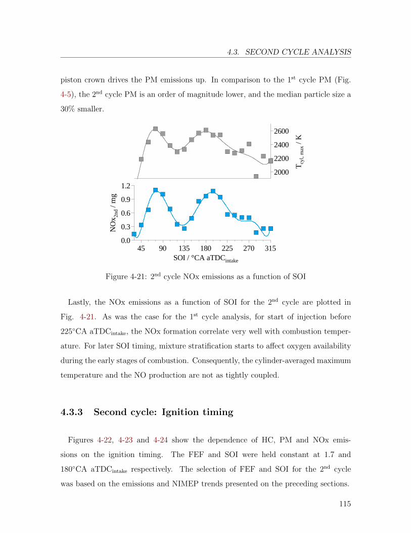
4.3. SECOND CYCLE ANALYSIS
piston crown drives the PM emissions up. In comparison to the 1st cycle PM (Fig.
4-5), the 2nd cycle PM is an order of magnitude lower, and the median particle size a
30% smaller.N
Ox 2
nd /
mg
0.0
0.3
0.6
0.9
1.2
SOI / °CA aTDCintake
45 90 135 180 225 270 315
Tcy
l, m
ax /
K
2000
2200
2400
2600
Figure 4-21: 2nd cycle NOx emissions as a function of SOI
Lastly, the NOx emissions as a function of SOI for the 2nd cycle are plotted in
Fig. 4-21. As was the case for the 1st cycle analysis, for start of injection before
225◦CA aTDCintake, the NOx formation correlate very well with combustion temper-
ature. For later SOI timing, mixture stratification starts to affect oxygen availability
during the early stages of combustion. Consequently, the cylinder-averaged maximum
temperature and the NO production are not as tightly coupled.
4.3.3 Second cycle: Ignition timing
Figures 4-22, 4-23 and 4-24 show the dependence of HC, PM and NOx emis-
sions on the ignition timing. The FEF and SOI were held constant at 1.7 and
180◦CA aTDCintake respectively. The selection of FEF and SOI for the 2nd cycle
was based on the emissions and NIMEP trends presented on the preceding sections.
115
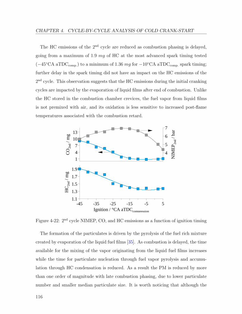
CHAPTER 4. CYCLE-BY-CYCLE ANALYSIS OF COLD CRANK-START
The HC emissions of the 2nd cycle are reduced as combustion phasing is delayed,
going from a maximum of 1.9 mg of HC at the most advanced spark timing tested
(−45◦CA aTDCcomp.) to a minimum of 1.36 mg for −10◦CA aTDCcomp. spark timing;
further delay in the spark timing did not have an impact on the HC emissions of the
2nd cycle. This observation suggests that the HC emissions during the initial cranking
cycles are impacted by the evaporation of liquid films after end of combustion. Unlike
the HC stored in the combustion chamber crevices, the fuel vapor from liquid films
is not premixed with air, and its oxidation is less sensitive to increased post-flame
temperatures associated with the combustion retard.
CO
2nd /
mg
1
4
7
10
13
HC
2nd /
mg
1.1
1.3
1.5
1.7
1.9
Ignition / °CA aTDCcompression
-45 -35 -25 -15 -5 5
NIM
EP
2nd /
ba
r
4
5
6
7
Figure 4-22: 2nd cycle NIMEP, CO, and HC emissions as a function of ignition timing
The formation of the particulates is driven by the pyrolysis of the fuel rich mixture
created by evaporation of the liquid fuel films [35]. As combustion is delayed, the time
available for the mixing of the vapor originating from the liquid fuel films increases
while the time for particulate nucleation through fuel vapor pyrolysis and accumu-
lation through HC condensation is reduced. As a result the PM is reduced by more
than one order of magnitude with late combustion phasing, due to lower particulate
number and smaller median particulate size. It is worth noticing that although the
116
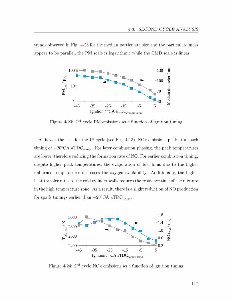
4.3. SECOND CYCLE ANALYSIS
trends observed in Fig. 4-23 for the median particulate size and the particulate mass
appear to be parallel, the PM scale is logarithmic while the CMD scale is linear.
PM
2nd /
µg
1
10
100
Ignition / °CA aTDCcompression
-45 -35 -25 -15 -5 5 Med
ian
dia
me
ter
/ nm
40
70
100
130
Figure 4-23: 2nd cycle PM emissions as a function of ignition timing
As it was the case for the 1st cycle (see Fig. 4-13), NOx emissions peak at a spark
timing of −20◦CA aTDCcomp.. For later combustion phasing, the peak temperatures
are lower, therefore reducing the formation rate of NO. For earlier combustion timing,
despite higher peak temperatures, the evaporation of fuel films due to the higher
unburned temperatures decreases the oxygen availability. Additionally, the higher
heat transfer rates to the cold cylinder walls reduces the residence time of the mixture
in the high temperature zone. As a result, there is a slight reduction of NO production
for spark timings earlier than −20◦CA aTDCcomp..
NO
x 2nd
/ m
g
0.2
0.6
1.0
1.4
1.8
Tcy
l, m
ax /
K
2400
2600
2800
3000
Ignition / °CA aTDCcompression
-45 -35 -25 -15 -5 5
Figure 4-24: 2nd cycle NOx emissions as a function of ignition timing
117
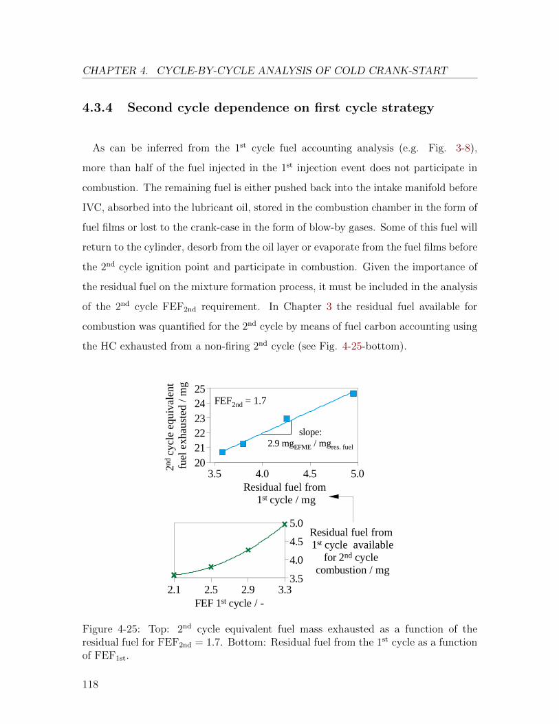
CHAPTER 4. CYCLE-BY-CYCLE ANALYSIS OF COLD CRANK-START
4.3.4 Second cycle dependence on first cycle strategy
As can be inferred from the 1st cycle fuel accounting analysis (e.g. Fig. 3-8),
more than half of the fuel injected in the 1st injection event does not participate in
combustion. The remaining fuel is either pushed back into the intake manifold before
IVC, absorbed into the lubricant oil, stored in the combustion chamber in the form of
fuel films or lost to the crank-case in the form of blow-by gases. Some of this fuel will
return to the cylinder, desorb from the oil layer or evaporate from the fuel films before
the 2nd cycle ignition point and participate in combustion. Given the importance of
the residual fuel on the mixture formation process, it must be included in the analysis
of the 2nd cycle FEF2nd requirement. In Chapter 3 the residual fuel available for
combustion was quantified for the 2nd cycle by means of fuel carbon accounting using
the HC exhausted from a non-firing 2nd cycle (see Fig. 4-25-bottom).
FEF2nd = 1.7
slope:2.9 mgEFME / mgres. fuel
Residual fuel from 1st cycle available
for 2nd cycle combustion / mg
3.5
4.0
4.5
5.0
FEF 1st cycle / -2.1 2.5 2.9 3.3
2nd c
ycle
equ
ival
ent
fuel
exh
aust
ed /
mg
202122232425
Residual fuel from 1st cycle / mg
3.5 4.0 4.5 5.0
Figure 4-25: Top: 2nd cycle equivalent fuel mass exhausted as a function of theresidual fuel for FEF2nd = 1.7. Bottom: Residual fuel from the 1st cycle as a functionof FEF1st.
118
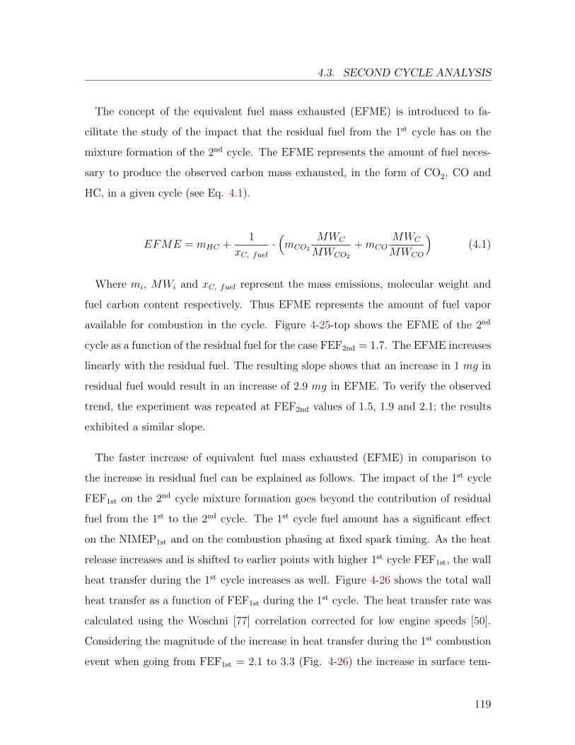
4.3. SECOND CYCLE ANALYSIS
The concept of the equivalent fuel mass exhausted (EFME) is introduced to fa-
cilitate the study of the impact that the residual fuel from the 1st cycle has on the
mixture formation of the 2nd cycle. The EFME represents the amount of fuel neces-
sary to produce the observed carbon mass exhausted, in the form of CO2, CO and
HC, in a given cycle (see Eq. 4.1).
EFME = mHC +1
xC, fuel·(mCO2
MWC
MWCO2
+mCOMWC
MWCO
)(4.1)
Where mi, MWi and xC, fuel represent the mass emissions, molecular weight and
fuel carbon content respectively. Thus EFME represents the amount of fuel vapor
available for combustion in the cycle. Figure 4-25-top shows the EFME of the 2nd
cycle as a function of the residual fuel for the case FEF2nd = 1.7. The EFME increases
linearly with the residual fuel. The resulting slope shows that an increase in 1 mg in
residual fuel would result in an increase of 2.9 mg in EFME. To verify the observed
trend, the experiment was repeated at FEF2nd values of 1.5, 1.9 and 2.1; the results
exhibited a similar slope.
The faster increase of equivalent fuel mass exhausted (EFME) in comparison to
the increase in residual fuel can be explained as follows. The impact of the 1st cycle
FEF1st on the 2nd cycle mixture formation goes beyond the contribution of residual
fuel from the 1st to the 2nd cycle. The 1st cycle fuel amount has a significant effect
on the NIMEP1st and on the combustion phasing at fixed spark timing. As the heat
release increases and is shifted to earlier points with higher 1st cycle FEF1st, the wall
heat transfer during the 1st cycle increases as well. Figure 4-26 shows the total wall
heat transfer as a function of FEF1st during the 1st cycle. The heat transfer rate was
calculated using the Woschni [77] correlation corrected for low engine speeds [50].
Considering the magnitude of the increase in heat transfer during the 1st combustion
event when going from FEF1st = 2.1 to 3.3 (Fig. 4-26) the increase in surface tem-
119
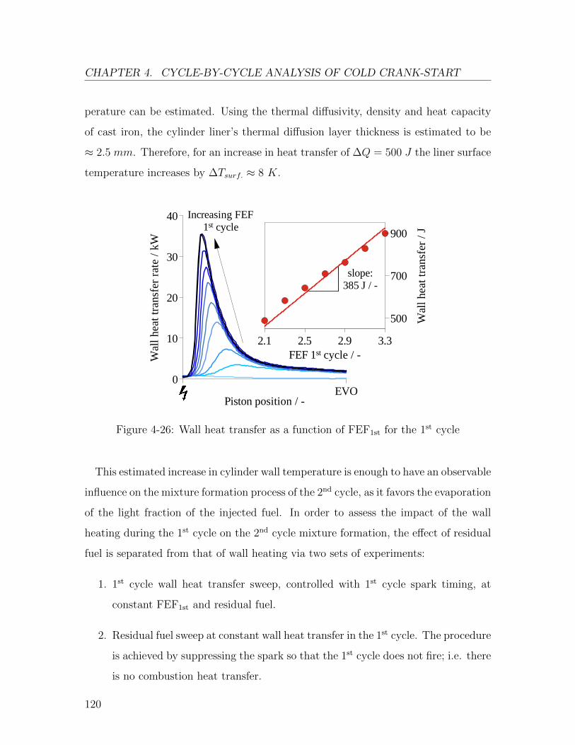
CHAPTER 4. CYCLE-BY-CYCLE ANALYSIS OF COLD CRANK-START
perature can be estimated. Using the thermal diffusivity, density and heat capacity
of cast iron, the cylinder liner’s thermal diffusion layer thickness is estimated to be
≈ 2.5 mm. Therefore, for an increase in heat transfer of ∆Q = 500 J the liner surface
temperature increases by ∆Tsurf. ≈ 8 K.
Wal
l hea
t tra
nsfe
r ra
te /
kW
0
10
20
30
40
Piston position / -EVO
Increasing FEF1st cycle
Wal
l hea
t tra
nsfe
r / J
500
700
900
FEF 1st cycle / -2.1 2.5 2.9 3.3
slope:385 J / -
Figure 4-26: Wall heat transfer as a function of FEF1st for the 1st cycle
This estimated increase in cylinder wall temperature is enough to have an observable
influence on the mixture formation process of the 2nd cycle, as it favors the evaporation
of the light fraction of the injected fuel. In order to assess the impact of the wall
heating during the 1st cycle on the 2nd cycle mixture formation, the effect of residual
fuel is separated from that of wall heating via two sets of experiments:
1. 1st cycle wall heat transfer sweep, controlled with 1st cycle spark timing, at
constant FEF1st and residual fuel.
2. Residual fuel sweep at constant wall heat transfer in the 1st cycle. The procedure
is achieved by suppressing the spark so that the 1st cycle does not fire; i.e. there
is no combustion heat transfer.
120
4.3. SECOND CYCLE ANALYSIS
As shown in Fig. 4-27, for the first set of experiments, the wall heat transfer
increases with spark advance; at the same time the residual fuel mass remains ap-
proximately unchanged. The spark timing sweep range was selected to achieve a
similar heat transfer range as the one resulting from the 1st cycle FEF1st sweep. The
dependence of the 2nd cycle equivalent fuel mass exhausted as a function of the 1st
cycle total wall heat transfer for the case FEF2nd = 1.7 is shown in Fig. 4-28. As the
1st cycle wall heat transfer is increased (through 1st cycle spark advance) the 2nd cycle
EFME increases. Using a linear fit, the slope indicates that a 100 J increase in heat
transfer would result in a 1 mg increase in EFME. To further confirm the validity of
these observations, the experiment was carried out at FEF2nd values of 1.5, 1.9 and
2.1; a similar dependence of the EFME on the 1st cycle heat transfer was observed in
all cases.
Wal
l he
at
tra
nsfe
r ra
te /
kW
0
10
20
30
40
Piston position / -EVO
More spark adv.1st cycle
Wal
l he
at
tra
nsfe
r 1s
t cyc
le /
J
550
700
850
1000
Ignition 1st cycle / °CA aTDCcomp.
-45 -35 -25 -15
Res
idua
l HC
fr
om 1
st c
ycle
/ m
g
3
4
5
Figure 4-27: Wall heat transfer and residual fuel as a function of spark timing for the1st cycle
121
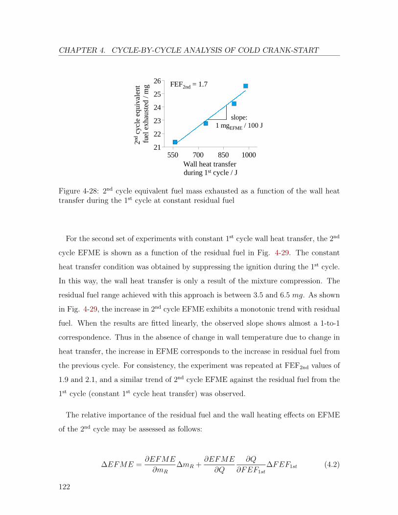
CHAPTER 4. CYCLE-BY-CYCLE ANALYSIS OF COLD CRANK-START
slope:1 mgEFME / 100 J
2nd c
ycle
equ
ival
ent
fuel
exh
aust
ed /
mg
21
22
23
24
25
26
Wall heat transfer during 1st cycle / J
550 700 850 1000
FEF2nd = 1.7
Figure 4-28: 2nd cycle equivalent fuel mass exhausted as a function of the wall heattransfer during the 1st cycle at constant residual fuel
For the second set of experiments with constant 1st cycle wall heat transfer, the 2nd
cycle EFME is shown as a function of the residual fuel in Fig. 4-29. The constant
heat transfer condition was obtained by suppressing the ignition during the 1st cycle.
In this way, the wall heat transfer is only a result of the mixture compression. The
residual fuel range achieved with this approach is between 3.5 and 6.5 mg. As shown
in Fig. 4-29, the increase in 2nd cycle EFME exhibits a monotonic trend with residual
fuel. When the results are fitted linearly, the observed slope shows almost a 1-to-1
correspondence. Thus in the absence of change in wall temperature due to change in
heat transfer, the increase in EFME corresponds to the increase in residual fuel from
the previous cycle. For consistency, the experiment was repeated at FEF2nd values of
1.9 and 2.1, and a similar trend of 2nd cycle EFME against the residual fuel from the
1st cycle (constant 1st cycle heat transfer) was observed.
The relative importance of the residual fuel and the wall heating effects on EFME
of the 2nd cycle may be assessed as follows:
∆EFME =∂EFME
∂mR
∆mR +∂EFME
∂Q
∂Q
∂FEF1st
∆FEF1st (4.2)
122
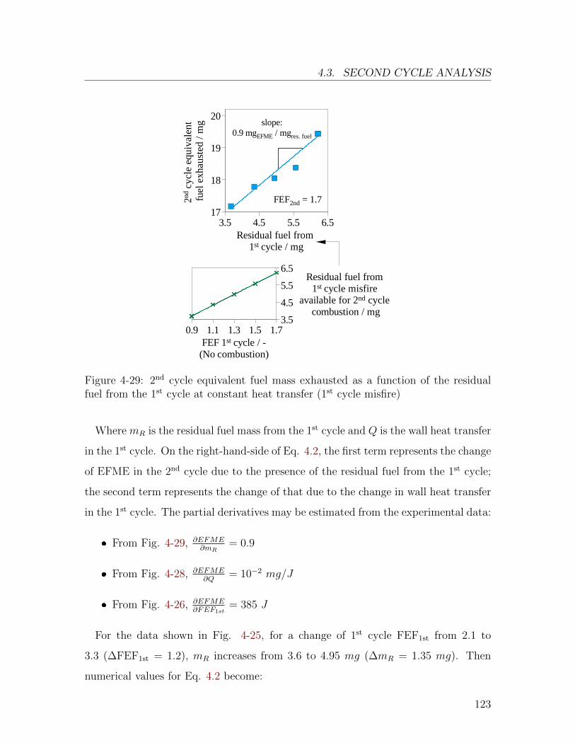
4.3. SECOND CYCLE ANALYSIS
Residual fuel from 1st cycle misfire
available for 2nd cycle combustion / mg
3.5
4.5
5.5
6.5
FEF 1st cycle / -(No combustion)
0.9 1.1 1.3 1.5 1.7
2nd c
ycle
equ
ival
ent
fuel
exh
aust
ed /
mg
17
18
19
20
Residual fuel from 1st cycle / mg
3.5 4.5 5.5 6.5
slope:0.9 mgEFME / mgres. fuel
FEF2nd = 1.7
Figure 4-29: 2nd cycle equivalent fuel mass exhausted as a function of the residualfuel from the 1st cycle at constant heat transfer (1st cycle misfire)
Where mR is the residual fuel mass from the 1st cycle and Q is the wall heat transfer
in the 1st cycle. On the right-hand-side of Eq. 4.2, the first term represents the change
of EFME in the 2nd cycle due to the presence of the residual fuel from the 1st cycle;
the second term represents the change of that due to the change in wall heat transfer
in the 1st cycle. The partial derivatives may be estimated from the experimental data:
� From Fig. 4-29, ∂EFME∂mR
= 0.9
� From Fig. 4-28, ∂EFME∂Q
= 10−2 mg/J
� From Fig. 4-26, ∂EFME∂FEF1st
= 385 J
For the data shown in Fig. 4-25, for a change of 1st cycle FEF1st from 2.1 to
3.3 (∆FEF1st = 1.2), mR increases from 3.6 to 4.95 mg (∆mR = 1.35 mg). Then
numerical values for Eq. 4.2 become:
123
CHAPTER 4. CYCLE-BY-CYCLE ANALYSIS OF COLD CRANK-START
∆EFME = 1.22 mg + 4.62 mg = 5.84 mg (4.3)
The above value is in line with the observed value of ∆EFME = 4.1 mg in Fig.
4-25. More importantly, Eq. 4.3 shows that the effect of the change of the wall heat
transfer in the 1st cycle on the 2nd cycle EFME is approximately 4 times that of the
residual fuel amount.
4.4 Third cycle analysis
Closing the cycle-by-cycle analysis, this section focuses on the 3rd engine cycle
during crank-start. In comparison to the preceding cycles, the 3rd cycle mixture
formation is improved due to the higher engine speed, reduced amount of injected
fuel from the lower intake manifold pressure, warmer cylinder walls and increased
fraction of residual fuel and gases. As it was done in the preceding section, the
analysis is focused on the start of injection (SOI), fuel enrichment factor (FEF), and
ignition timing using a one-variable-at-a-time approach. The swept ranges can be
found in Table 4.5.
Parameter Sweep range Nominal value
SOI [◦CA aTDCintake] 30 − 315 ∆ = 15 180FEF [−] 1.3 − 1.9 ∆ = 0.2 1.5Spark [◦CA aTDCcomp.] −45 − −5 ∆ = 5 -10
Table 4.5: Experimental scope for the 3rd cycle emissions
Once again, to decouple the effects of the 1st and 2nd cycle injection strategy on
the 3rd cycle emission analysis, the 1st and 2nd cycle strategies were kept constant as
shown in Table 4.6.
124
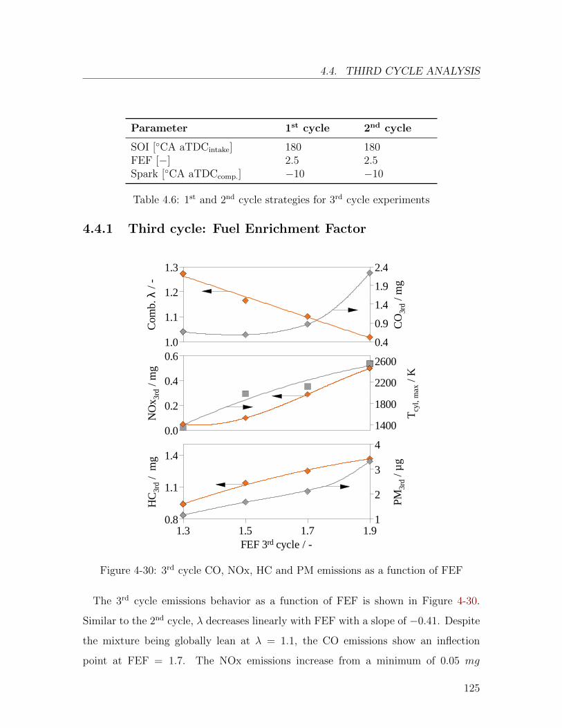
4.4. THIRD CYCLE ANALYSIS
Parameter 1st cycle 2nd cycle
SOI [◦CA aTDCintake] 180 180FEF [−] 2.5 2.5Spark [◦CA aTDCcomp.] −10 −10
Table 4.6: 1st and 2nd cycle strategies for 3rd cycle experiments
4.4.1 Third cycle: Fuel Enrichment Factor
FEF 3rd cycle / -1.3 1.5 1.7 1.9
HC
3rd
/ m
g
0.8
1.1
1.4
CO
3rd
/ mg
0.4
0.9
1.4
1.9
2.4
PM
3rd
/ µg
1
2
3
4
Com
b. λ
/ -
1.0
1.1
1.2
1.3
Tcy
l, m
ax /
K1400
1800
2200
2600
NO
x 3rd /
mg
0.0
0.2
0.4
0.6
Figure 4-30: 3rd cycle CO, NOx, HC and PM emissions as a function of FEF
The 3rd cycle emissions behavior as a function of FEF is shown in Figure 4-30.
Similar to the 2nd cycle, λ decreases linearly with FEF with a slope of −0.41. Despite
the mixture being globally lean at λ = 1.1, the CO emissions show an inflection
point at FEF = 1.7. The NOx emissions increase from a minimum of 0.05 mg
125
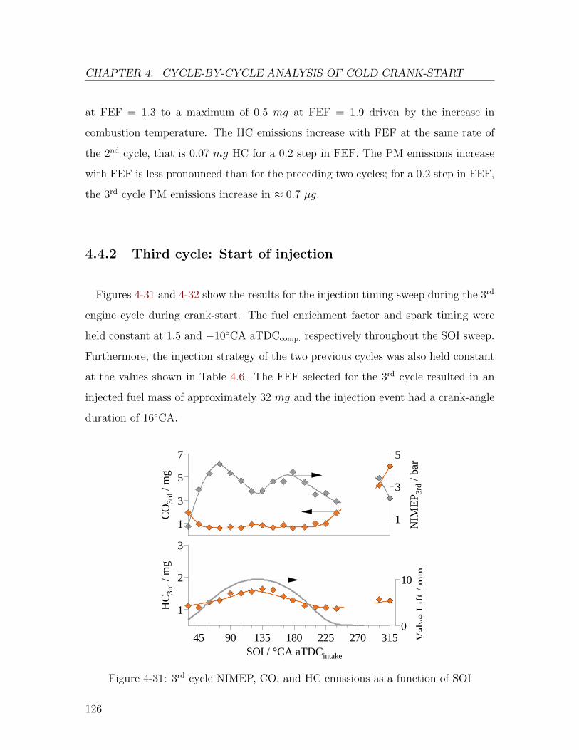
CHAPTER 4. CYCLE-BY-CYCLE ANALYSIS OF COLD CRANK-START
at FEF = 1.3 to a maximum of 0.5 mg at FEF = 1.9 driven by the increase in
combustion temperature. The HC emissions increase with FEF at the same rate of
the 2nd cycle, that is 0.07 mg HC for a 0.2 step in FEF. The PM emissions increase
with FEF is less pronounced than for the preceding two cycles; for a 0.2 step in FEF,
the 3rd cycle PM emissions increase in ≈ 0.7 µg.
4.4.2 Third cycle: Start of injection
Figures 4-31 and 4-32 show the results for the injection timing sweep during the 3rd
engine cycle during crank-start. The fuel enrichment factor and spark timing were
held constant at 1.5 and −10◦CA aTDCcomp. respectively throughout the SOI sweep.
Furthermore, the injection strategy of the two previous cycles was also held constant
at the values shown in Table 4.6. The FEF selected for the 3rd cycle resulted in an
injected fuel mass of approximately 32 mg and the injection event had a crank-angle
duration of 16◦CA.N
IME
P3r
d / b
ar
1
3
5
HC
3rd
/ mg
1
2
3
SOI / °CA aTDCintake
45 90 135 180 225 270 315
CO
3rd
/ mg
1
3
5
7
Val
ve L
ift /
mm
0
10
Figure 4-31: 3rd cycle NIMEP, CO, and HC emissions as a function of SOI
126
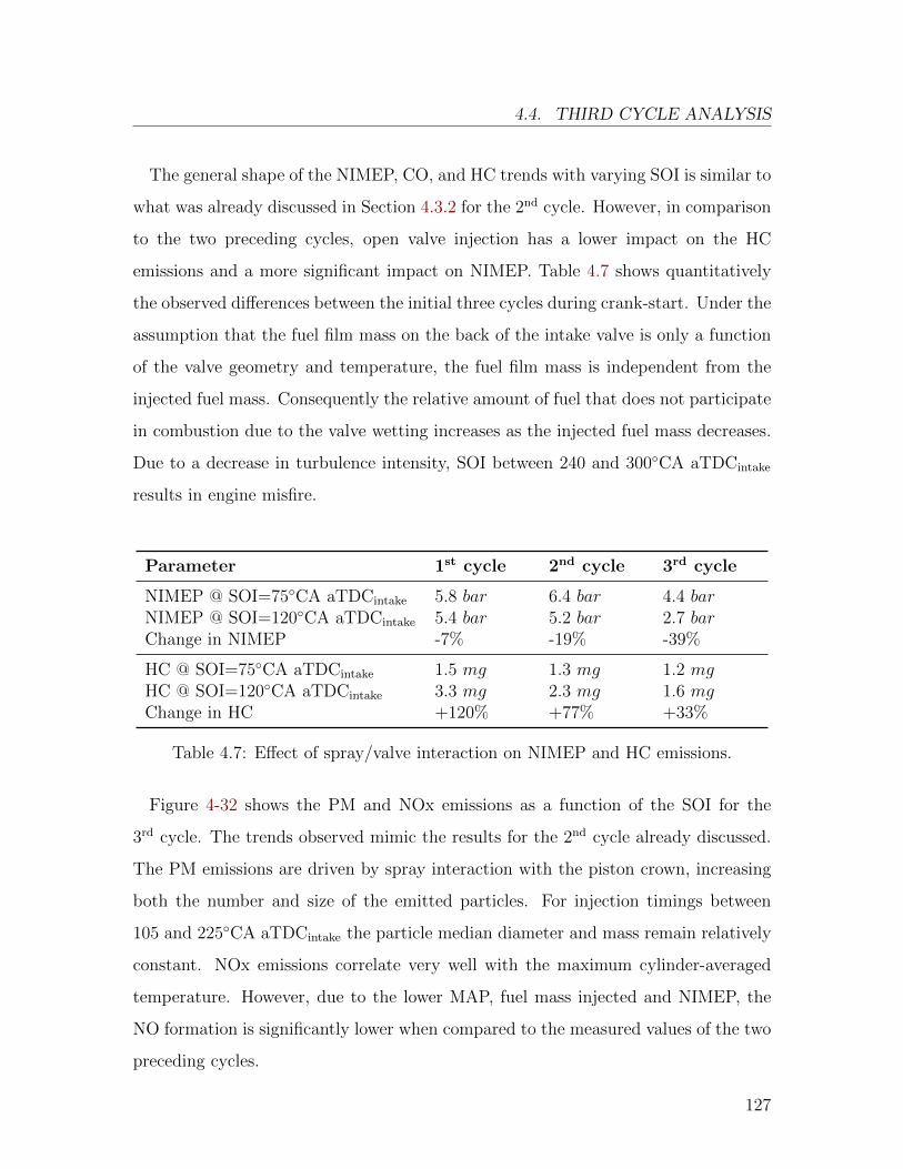
4.4. THIRD CYCLE ANALYSIS
The general shape of the NIMEP, CO, and HC trends with varying SOI is similar to
what was already discussed in Section 4.3.2 for the 2nd cycle. However, in comparison
to the two preceding cycles, open valve injection has a lower impact on the HC
emissions and a more significant impact on NIMEP. Table 4.7 shows quantitatively
the observed differences between the initial three cycles during crank-start. Under the
assumption that the fuel film mass on the back of the intake valve is only a function
of the valve geometry and temperature, the fuel film mass is independent from the
injected fuel mass. Consequently the relative amount of fuel that does not participate
in combustion due to the valve wetting increases as the injected fuel mass decreases.
Due to a decrease in turbulence intensity, SOI between 240 and 300◦CA aTDCintake
results in engine misfire.
Parameter 1st cycle 2nd cycle 3rd cycle
NIMEP @ SOI=75◦CA aTDCintake 5.8 bar 6.4 bar 4.4 barNIMEP @ SOI=120◦CA aTDCintake 5.4 bar 5.2 bar 2.7 barChange in NIMEP -7% -19% -39%
HC @ SOI=75◦CA aTDCintake 1.5 mg 1.3 mg 1.2 mgHC @ SOI=120◦CA aTDCintake 3.3 mg 2.3 mg 1.6 mgChange in HC +120% +77% +33%
Table 4.7: Effect of spray/valve interaction on NIMEP and HC emissions.
Figure 4-32 shows the PM and NOx emissions as a function of the SOI for the
3rd cycle. The trends observed mimic the results for the 2nd cycle already discussed.
The PM emissions are driven by spray interaction with the piston crown, increasing
both the number and size of the emitted particles. For injection timings between
105 and 225◦CA aTDCintake the particle median diameter and mass remain relatively
constant. NOx emissions correlate very well with the maximum cylinder-averaged
temperature. However, due to the lower MAP, fuel mass injected and NIMEP, the
NO formation is significantly lower when compared to the measured values of the two
preceding cycles.
127
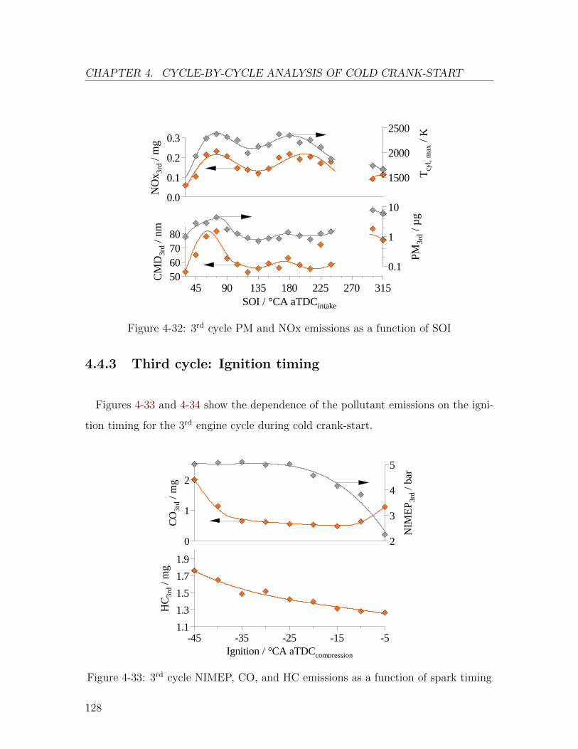
CHAPTER 4. CYCLE-BY-CYCLE ANALYSIS OF COLD CRANK-START
CM
D3r
d / n
m
50607080
SOI / °CA aTDCintake
45 90 135 180 225 270 315
PM
3rd
/ µg
0.1
1
10
NO
x 3rd /
mg
0.0
0.1
0.2
0.3
Tcy
l, m
ax /
K
1500
2000
2500
Figure 4-32: 3rd cycle PM and NOx emissions as a function of SOI
4.4.3 Third cycle: Ignition timing
Figures 4-33 and 4-34 show the dependence of the pollutant emissions on the igni-
tion timing for the 3rd engine cycle during cold crank-start.
CO
3rd
/ mg
0
1
2
HC
3rd
/ mg
1.1
1.3
1.5
1.7
1.9
Ignition / °CA aTDCcompression
-45 -35 -25 -15 -5
NIM
EP
3rd
/ ba
r
2
3
4
5
Figure 4-33: 3rd cycle NIMEP, CO, and HC emissions as a function of spark timing
128
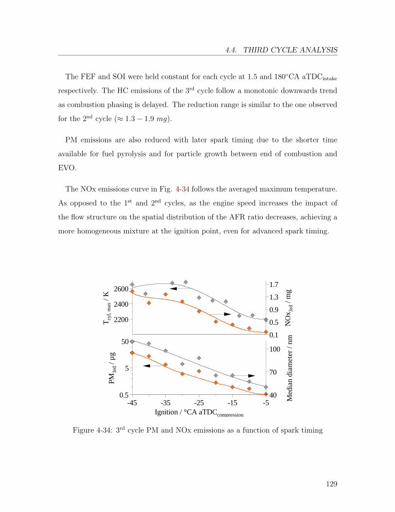
4.4. THIRD CYCLE ANALYSIS
The FEF and SOI were held constant for each cycle at 1.5 and 180◦CA aTDCintake
respectively. The HC emissions of the 3rd cycle follow a monotonic downwards trend
as combustion phasing is delayed. The reduction range is similar to the one observed
for the 2nd cycle (≈ 1.3− 1.9 mg).
PM emissions are also reduced with later spark timing due to the shorter time
available for fuel pyrolysis and for particle growth between end of combustion and
EVO.
The NOx emissions curve in Fig. 4-34 follows the averaged maximum temperature.
As opposed to the 1st and 2nd cycles, as the engine speed increases the impact of
the flow structure on the spatial distribution of the AFR ratio decreases, achieving a
more homogeneous mixture at the ignition point, even for advanced spark timing.
PM
3rd
/ µg
0.5
5
50
Ignition / °CA aTDCcompression
-45 -35 -25 -15 -5 Med
ian
dia
me
ter
/ nm
40
70
100
Tcy
l, m
ax /
K
2200
2400
2600N
Ox 3
rd /
mg
0.1
0.5
0.9
1.3
1.7
Figure 4-34: 3rd cycle PM and NOx emissions as a function of spark timing
129
CHAPTER 4. CYCLE-BY-CYCLE ANALYSIS OF COLD CRANK-START
4.5 Findings
The effects of fuel amount, injection timing and spark timing on the HC and PM
emissions of the initial 3 cycles during cold crank-start were studied in a wall guided
gasoline direct injection engine. The main results can be summarized as follows:
� The adverse conditions of temperature and charge motion during cold crank-
start result in mixture inhomogeneity. Consequently, aiming for an overall
combustion λ of 1 is not a viable strategy as it increases the CO, HC and
PM emissions. The amount of fuel injected needs to be large enough to reduce
the risk of misfire or partial burn, and sufficiently small to control the engine
out emissions. The results show that the optimum enrichment for the initial 3
cycles are FEF1st = 2.5, FEF2nd = 1.7 and FEF3rd = 1.5.
� The sensitivity of the HC emissions to the FEF is roughly the same for all
3 cycles, while the PM sensitivity decreases significantly as the cycle number
increases. In a similar way, the HC emissions for the initial 3 cycles are in the
same order of magnitude; between 1 and 1.5 mg/cyl./cycle. In contrast, the
PM emissions per cycle are reduced in more than an order of magnitude as the
crank-start progresses form the 1st to the 3rd cycle.
� The FEF history has an influence on the mixture formation through two mech-
anisms. First, as the FEF of previous cycles increases, so does the residual fuel
mass. Second, the amount and point of heat release for the previous cycles is a
function of FEF. The heat release increase of the previous cycles translates into
wall heating, impacting the fuel evaporation and mixture formation process.
� The SOI selection for minimizing the pollutant emissions presents a tradeoff.
The lowest HC emissions are achieved for SOI during the first half of the intake
stroke, for intake valve lifts lower than 5 mm. Contrary, the minimum PM
130
4.5. FINDINGS
emissions are achieved for SOI during the intake stroke and the intake valve lift
greater than 5 mm. Injection during the early compression stroke results in a
good compromise for both HC and PM emissions.
� The effect of fuel spray interaction with the intake valve in HC emissions is
reduced as the crank-start progresses form the 1st to the 3rd cycle. In contrast,
its impact of NIMEP increases.
� The HC emissions of the 1st cycle are insensitive to combustion phasing in
the range of interest. For the 2nd and 3rd cycles, spark timing retard re-
sults in approximately a 30% reduction as the spark timing goes from −45
to 10◦CA aTDCcomp.. For the 3 cycles studied, the observed PM reduction with
combustion retard is larger than an order of magnitude as the spark timing is
delayed from −45 to 10◦CA aTDCcomp..
� NOx emissions are driven by combustion temperature and correlate well with
the maximum cylinder-averaged temperature. In the case of mixture inhomo-
geneities due to mixture stratification or flow structure, rich zone can result in a
reduction of oxygen availability and consequently lead to lower NOx emissions.
131

– Intentionally left blank –
Chapter 5
Valve timing effect on crank-start
The goal of this chapter is to assess the potential of unconventional valve timings for
reducing the engine-out hydrocarbon, particulate matter and nitrogen oxides emis-
sions during the cold crank-start of a gasoline direct injection engine. With variable
valve timing (VVT) systems, the selection of the de-energized position (parked posi-
tion) of the camshafts is limited by the authority of the phasing system (in ◦CA) and
the desired maximum intake advance and exhaust retard during warm operation. As
the authority of VVT systems increases, new camshaft parked positions become pos-
sible. The merit of these alternative parked positions for cold crank-start emissions
control is discussed in this chapter. The four different valve timing settings that were
studied in detail are as follows:
1. Baseline stock valve timing
2. Late intake opening/closing
3. Early exhaust opening/closing
4. Late intake phasing combined with early exhaust phasing
133
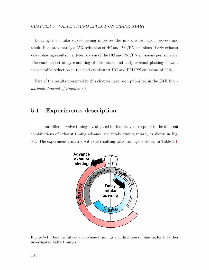
CHAPTER 5. VALVE TIMING EFFECT ON CRANK-START
Delaying the intake valve opening improves the mixture formation process and
results in approximately a 25% reduction of HC and PM/PN emissions. Early exhaust
valve phasing results in a deterioration of the HC and PM/PN emissions performance.
The combined strategy consisting of late intake and early exhaust phasing shows a
considerable reduction in the cold crank-start HC and PM/PN emissions of 30%.
Part of the results presented in this chapter have been published in the SAE Inter-
national Journal of Engines [63].
5.1 Experiments description
The four different valve timing investigated in this study correspond to the different
combinations of exhaust timing advance and intake timing retard, as shown in Fig.
5-1. The experimental matrix with the resulting valve timings is shown in Table 5.1.
Figure 5-1: Baseline intake and exhaust timings and direction of phasing for the otherinvestigated valve timings
134
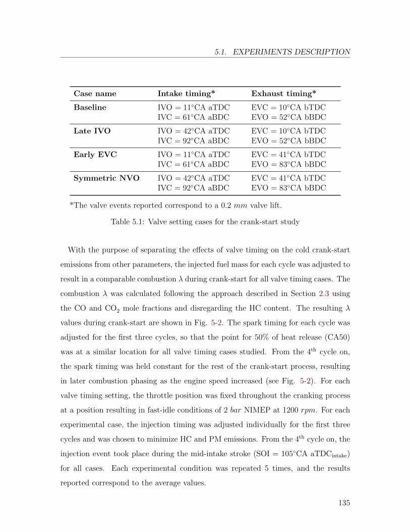
5.1. EXPERIMENTS DESCRIPTION
Case name Intake timing* Exhaust timing*
Baseline IVO = 11◦CA aTDC EVC = 10◦CA bTDCIVC = 61◦CA aBDC EVO = 52◦CA bBDC
Late IVO IVO = 42◦CA aTDC EVC = 10◦CA bTDCIVC = 92◦CA aBDC EVO = 52◦CA bBDC
Early EVC IVO = 11◦CA aTDC EVC = 41◦CA bTDCIVC = 61◦CA aBDC EVO = 83◦CA bBDC
Symmetric NVO IVO = 42◦CA aTDC EVC = 41◦CA bTDCIVC = 92◦CA aBDC EVO = 83◦CA bBDC
*The valve events reported correspond to a 0.2 mm valve lift.
Table 5.1: Valve setting cases for the crank-start study
With the purpose of separating the effects of valve timing on the cold crank-start
emissions from other parameters, the injected fuel mass for each cycle was adjusted to
result in a comparable combustion λ during crank-start for all valve timing cases. The
combustion λ was calculated following the approach described in Section 2.3 using
the CO and CO2 mole fractions and disregarding the HC content. The resulting λ
values during crank-start are shown in Fig. 5-2. The spark timing for each cycle was
adjusted for the first three cycles, so that the point for 50% of heat release (CA50)
was at a similar location for all valve timing cases studied. From the 4th cycle on,
the spark timing was held constant for the rest of the crank-start process, resulting
in later combustion phasing as the engine speed increased (see Fig. 5-2). For each
valve timing setting, the throttle position was fixed throughout the cranking process
at a position resulting in fast-idle conditions of 2 bar NIMEP at 1200 rpm. For each
experimental case, the injection timing was adjusted individually for the first three
cycles and was chosen to minimize HC and PM emissions. From the 4th cycle on, the
injection event took place during the mid-intake stroke (SOI = 105◦CA aTDCintake)
for all cases. Each experimental condition was repeated 5 times, and the results
reported correspond to the average values.
135
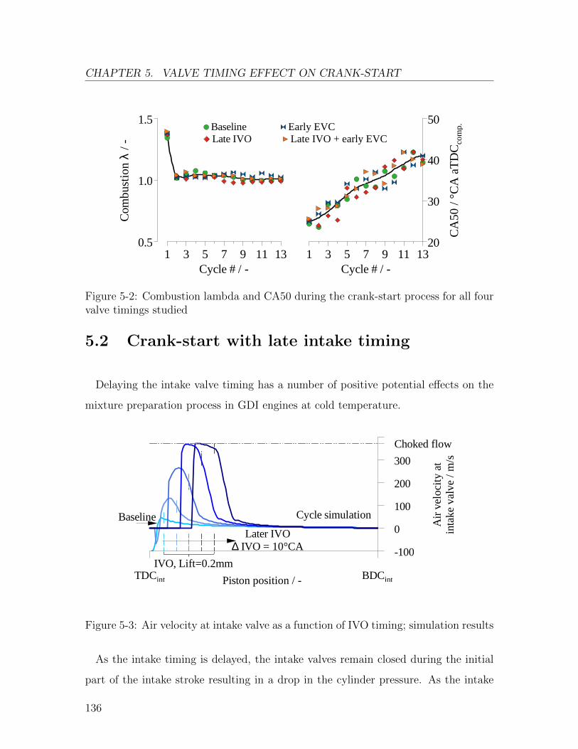
CHAPTER 5. VALVE TIMING EFFECT ON CRANK-START
Com
bus
tion
λ / -
0.5
1.0
1.5
Cycle # / -1 3 5 7 9 11 13
Baseline Early EVC Late IVO Late IVO + early EVC
CA
50
/ °C
A a
TD
C com
p.
20
30
40
50
Cycle # / -1 3 5 7 9 11 13
Figure 5-2: Combustion lambda and CA50 during the crank-start process for all fourvalve timings studied
5.2 Crank-start with late intake timing
Delaying the intake valve timing has a number of positive potential effects on the
mixture preparation process in GDI engines at cold temperature.
IVO, Lift=0.2mm
Air
velo
city
at
inta
ke v
alve
/ m
/sChoked flow
-100
0
100
200
300
Piston position / - TDCint BDCint
Later IVO∆ IVO = 10°CA
Baseline Cycle simulation
Figure 5-3: Air velocity at intake valve as a function of IVO timing; simulation results
As the intake timing is delayed, the intake valves remain closed during the initial
part of the intake stroke resulting in a drop in the cylinder pressure. As the intake
136
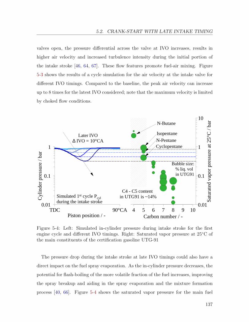
5.2. CRANK-START WITH LATE INTAKE TIMING
valves open, the pressure differential across the valve at IVO increases, results in
higher air velocity and increased turbulence intensity during the initial portion of
the intake stroke [46, 64, 67]. These flow features promote fuel-air mixing. Figure
5-3 shows the results of a cycle simulation for the air velocity at the intake valve for
different IVO timings. Compared to the baseline, the peak air velocity can increase
up to 8 times for the latest IVO considered; note that the maximum velocity is limited
by choked flow conditions.
Bubble size:% liq. vol in UTG91
Cyl
inde
r pr
ess
ure
/ b
ar
0.01
0.1
1
Piston position / - TDC 90°CA
Later IVO∆ IVO = 10°CA
Simulated 1st cycle Pcylduring the intake stroke S
atur
ate
d va
por
pre
ssur
e a
t 2
5°C
/ b
ar
0.01
0.1
1
10
Carbon number / -4 5 6 7 8 9 10
N-Butane
Isopentane
Cyclopentane
C4 - C5 content in UTG91 is ~14%
N-Pentane
Figure 5-4: Left: Simulated in-cylinder pressure during intake stroke for the firstengine cycle and different IVO timings. Right: Saturated vapor pressure at 25◦C ofthe main constituents of the certification gasoline UTG-91
The pressure drop during the intake stroke at late IVO timings could also have a
direct impact on the fuel spray evaporation. As the in-cylinder pressure decreases, the
potential for flash-boiling of the more volatile fraction of the fuel increases, improving
the spray breakup and aiding in the spray evaporation and the mixture formation
process [40, 66]. Figure 5-4 shows the saturated vapor pressure for the main fuel
137
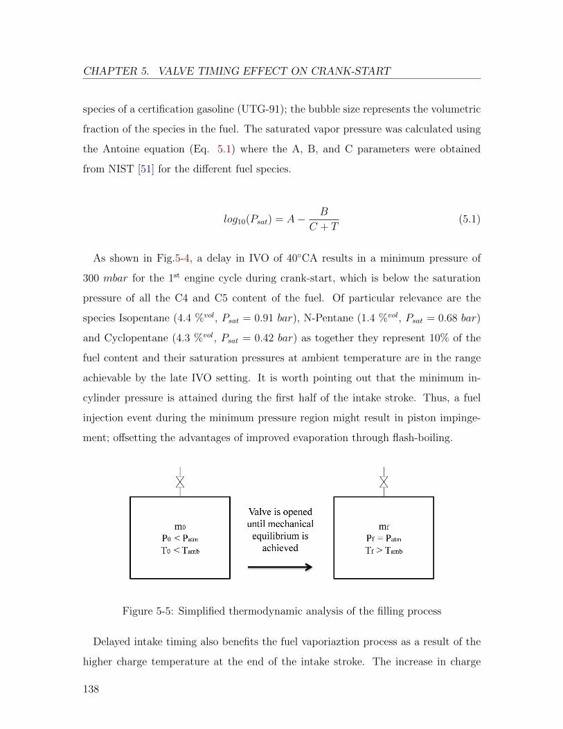
CHAPTER 5. VALVE TIMING EFFECT ON CRANK-START
species of a certification gasoline (UTG-91); the bubble size represents the volumetric
fraction of the species in the fuel. The saturated vapor pressure was calculated using
the Antoine equation (Eq. 5.1) where the A, B, and C parameters were obtained
from NIST [51] for the different fuel species.
log10(Psat) = A− B
C + T(5.1)
As shown in Fig.5-4, a delay in IVO of 40◦CA results in a minimum pressure of
300 mbar for the 1st engine cycle during crank-start, which is below the saturation
pressure of all the C4 and C5 content of the fuel. Of particular relevance are the
species Isopentane (4.4 %vol, Psat = 0.91 bar), N-Pentane (1.4 %vol, Psat = 0.68 bar)
and Cyclopentane (4.3 %vol, Psat = 0.42 bar) as together they represent 10% of the
fuel content and their saturation pressures at ambient temperature are in the range
achievable by the late IVO setting. It is worth pointing out that the minimum in-
cylinder pressure is attained during the first half of the intake stroke. Thus, a fuel
injection event during the minimum pressure region might result in piston impinge-
ment; offsetting the advantages of improved evaporation through flash-boiling.
Figure 5-5: Simplified thermodynamic analysis of the filling process
Delayed intake timing also benefits the fuel vaporiaztion process as a result of the
higher charge temperature at the end of the intake stroke. The increase in charge
138
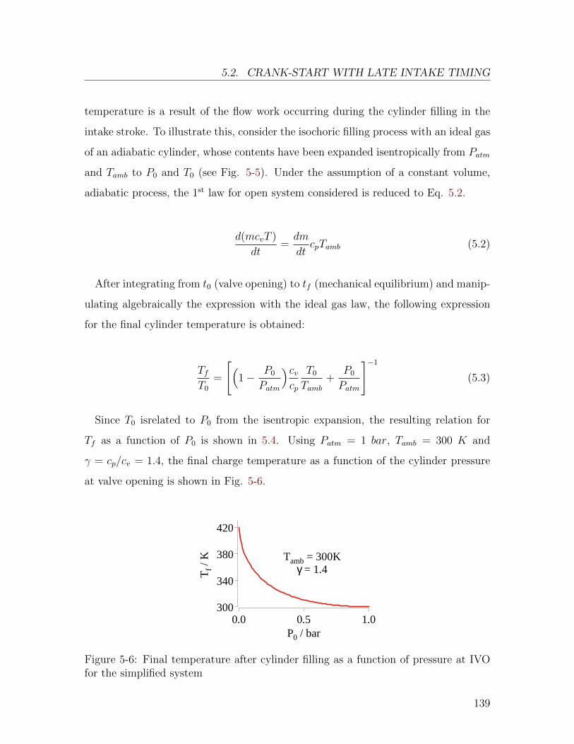
5.2. CRANK-START WITH LATE INTAKE TIMING
temperature is a result of the flow work occurring during the cylinder filling in the
intake stroke. To illustrate this, consider the isochoric filling process with an ideal gas
of an adiabatic cylinder, whose contents have been expanded isentropically from Patm
and Tamb to P0 and T0 (see Fig. 5-5). Under the assumption of a constant volume,
adiabatic process, the 1st law for open system considered is reduced to Eq. 5.2.
d(mcvT )
dt=dm
dtcpTamb (5.2)
After integrating from t0 (valve opening) to tf (mechanical equilibrium) and manip-
ulating algebraically the expression with the ideal gas law, the following expression
for the final cylinder temperature is obtained:
TfT0
=
[(1− P0
Patm
)cvcp
T0Tamb
+P0
Patm
]−1
(5.3)
Since T0 isrelated to P0 from the isentropic expansion, the resulting relation for
Tf as a function of P0 is shown in 5.4. Using Patm = 1 bar, Tamb = 300 K and
γ = cp/cv = 1.4, the final charge temperature as a function of the cylinder pressure
at valve opening is shown in Fig. 5-6.
Tf /
K
300
340
380
420
P0 / bar0.0 0.5 1.0
Tamb = 300Kγ = 1.4
Figure 5-6: Final temperature after cylinder filling as a function of pressure at IVOfor the simplified system
139
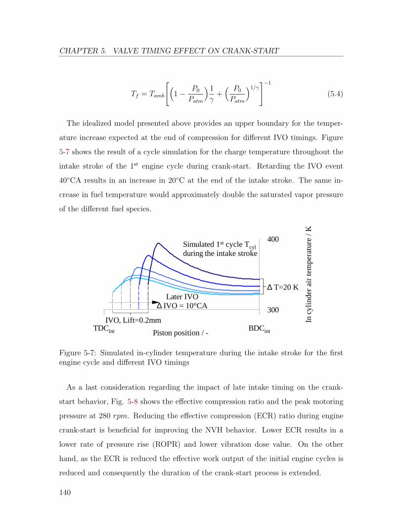
CHAPTER 5. VALVE TIMING EFFECT ON CRANK-START
Tf = Tamb
[(1− P0
Patm
)1
γ+( P0
Patm
)1/γ]−1
(5.4)
The idealized model presented above provides an upper boundary for the temper-
ature increase expected at the end of compression for different IVO timings. Figure
5-7 shows the result of a cycle simulation for the charge temperature throughout the
intake stroke of the 1st engine cycle during crank-start. Retarding the IVO event
40◦CA results in an increase in 20◦C at the end of the intake stroke. The same in-
crease in fuel temperature would approximately double the saturated vapor pressure
of the different fuel species.
IVO, Lift=0.2mm
Later IVO∆ IVO = 10°CA
Simulated 1st cycle Tcylduring the intake stroke
In c
ylin
der
air
te
mpe
ratu
re /
K
∆ T=20 K
300
400
Piston position / - TDCint BDCint
Figure 5-7: Simulated in-cylinder temperature during the intake stroke for the firstengine cycle and different IVO timings
As a last consideration regarding the impact of late intake timing on the crank-
start behavior, Fig. 5-8 shows the effective compression ratio and the peak motoring
pressure at 280 rpm. Reducing the effective compression (ECR) ratio during engine
crank-start is beneficial for improving the NVH behavior. Lower ECR results in a
lower rate of pressure rise (ROPR) and lower vibration dose value. On the other
hand, as the ECR is reduced the effective work output of the initial engine cycles is
reduced and consequently the duration of the crank-start process is extended.
140
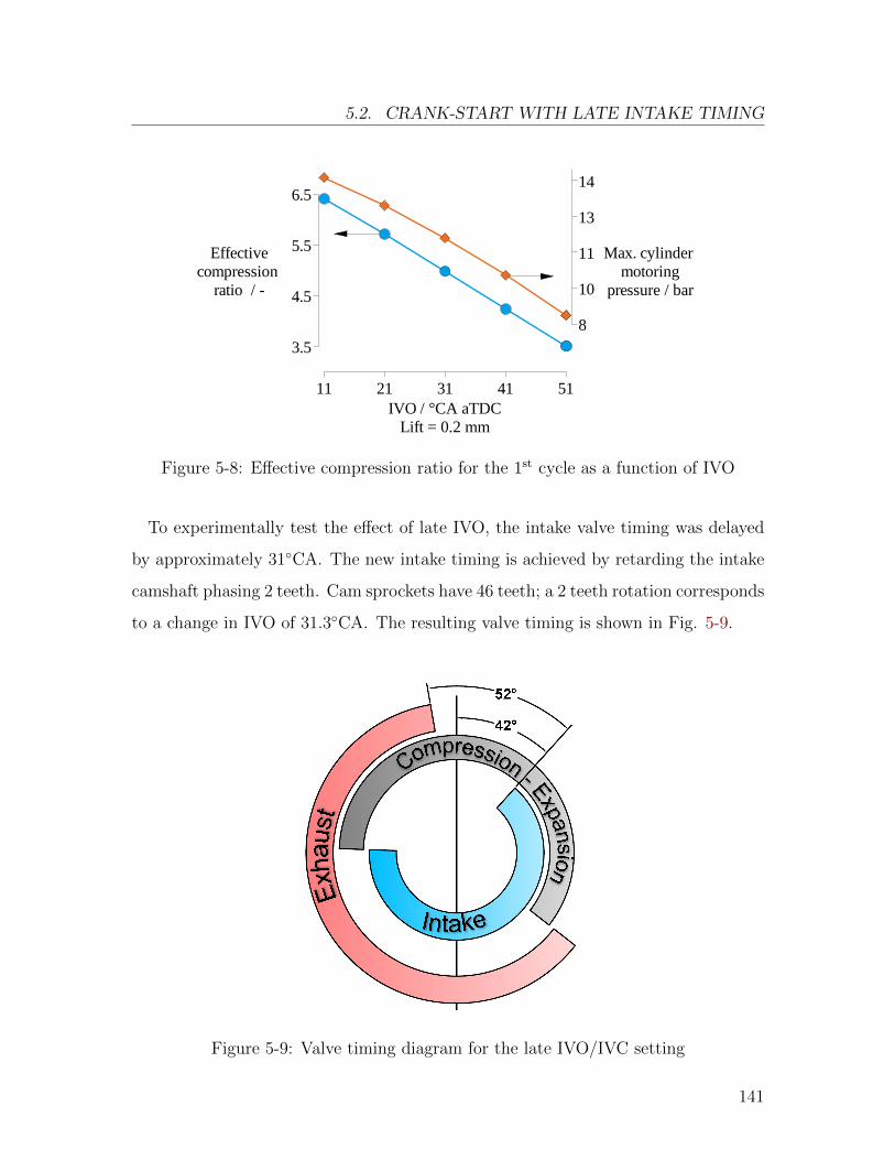
5.2. CRANK-START WITH LATE INTAKE TIMING
IVO / °CA aTDCLift = 0.2 mm
11 21 31 41 51
Effectivecompression
ratio / -
3.5
4.5
5.5
6.5
Max. cylinder motoring
pressure / bar
8
10
11
13
14
Figure 5-8: Effective compression ratio for the 1st cycle as a function of IVO
To experimentally test the effect of late IVO, the intake valve timing was delayed
by approximately 31◦CA. The new intake timing is achieved by retarding the intake
camshaft phasing 2 teeth. Cam sprockets have 46 teeth; a 2 teeth rotation corresponds
to a change in IVO of 31.3◦CA. The resulting valve timing is shown in Fig. 5-9.
Figure 5-9: Valve timing diagram for the late IVO/IVC setting
141
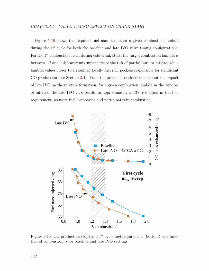
CHAPTER 5. VALVE TIMING EFFECT ON CRANK-START
Figure 5-10 shows the required fuel mass to attain a given combustion lambda
during the 1st cycle for both the baseline and late IVO valve timing configurations.
For the 1st combustion event during cold crank-start, the target combustion lambda is
between 1.2 and 1.4; leaner mixtures increase the risk of partial burn or misfire, while
lambda values closer to 1 result in locally fuel rich pockets responsible for significant
CO production (see Section 3.4). From the previous considerations about the impact
of late IVO on the mixture formation, for a given combustion lambda in the window
of interest, the late IVO case results in approximately a 13% reduction in the fuel
requirement, as more fuel evaporates and participates in combustion.
Fue
l ma
ss in
ject
ed
/ m
g
55
65
75
85
95
λ combustion / -0.8 1.0 1.2 1.4 1.6 1.8 2.0
Late IVO
First cycle mfuel sweep
CO
ma
ss e
xha
uste
d /
mg
0
1
2
3
4
5
6
7
8
Late IVO
Baseline Late IVO = 42°CA aTDC
Figure 5-10: CO production (top) and 1st cycle fuel requirement (bottom) as a func-tion of combustion λ for baseline and late IVO settings
142
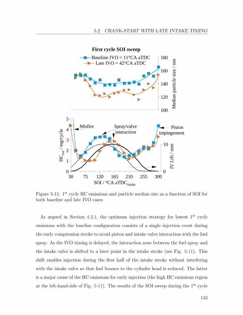
5.2. CRANK-START WITH LATE INTAKE TIMING
Baseline IVO = 11°CA aTDC Late IVO = 42°CA aTDC
First cycle SOI sweep
Piston impingement
Spray/valve interaction
Misfire
IV L
ift /
mm
0
10
HC
out /
mg/
cycl
e
0
1
2
3
4
5
SOI / °CA aTDCintake
30 75 120 165 210 255 300M
edia
n pa
rtic
le s
ize
/ n
m
100
120
140
160
180
Figure 5-11: 1st cycle HC emissions and particle median size as a function of SOI forboth baseline and late IVO cases
As argued in Section 4.2.1, the optimum injection strategy for lowest 1st cycle
emissions with the baseline configuration consists of a single injection event during
the early compression stroke to avoid piston and intake valve interaction with the fuel
spray. As the IVO timing is delayed, the interaction zone between the fuel spray and
the intake valve is shifted to a later point in the intake stroke (see Fig. 5-11). This
shift enables injection during the first half of the intake stroke without interfering
with the intake valve so that fuel bounce to the cylinder head is reduced. The latter
is a major cause of the HC emissions for early injection (the high HC emissions region
at the left-hand-side of Fig. 5-11). The results of the SOI sweep during the 1st cycle
143
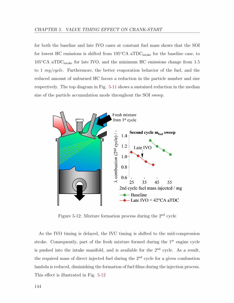
CHAPTER 5. VALVE TIMING EFFECT ON CRANK-START
for both the baseline and late IVO cases at constant fuel mass shows that the SOI
for lowest HC emissions is shifted from 195◦CA aTDCintake for the baseline case, to
105◦CA aTDCintake for late IVO, and the minimum HC emissions change from 1.5
to 1 mg/cycle. Furthermore, the better evaporation behavior of the fuel, and the
reduced amount of unburned HC favors a reduction in the particle number and size
respectively. The top diagram in Fig. 5-11 shows a sustained reduction in the median
size of the particle accumulation mode throughout the SOI sweep.
Figure 5-12: Mixture formation process during the 2nd cycle
As the IVO timing is delayed, the IVC timing is shifted to the mid-compression
stroke. Consequently, part of the fresh mixture formed during the 1st engine cycle
is pushed into the intake manifold, and is available for the 2nd cycle. As a result,
the required mass of direct injected fuel during the 2nd cycle for a given combustion
lambda is reduced, diminishing the formation of fuel films during the injection process.
This effect is illustrated in Fig. 5-12
144
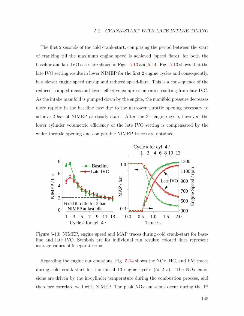
5.2. CRANK-START WITH LATE INTAKE TIMING
The first 2 seconds of the cold crank-start, comprising the period between the start
of cranking till the maximum engine speed is achieved (speed flare), for both the
baseline and late IVO cases are shown in Figs. 5-13 and 5-14. Fig. 5-13 shows that the
late IVO setting results in lower NIMEP for the first 2 engine cycles and consequently,
in a slower engine speed run-up and reduced speed-flare. This is a consequence of the
reduced trapped mass and lower effective compression ratio resulting from late IVC.
As the intake manifold is pumped down by the engine, the manifold pressure decreases
more rapidly in the baseline case due to the narrower throttle opening necessary to
achieve 2 bar of NIMEP at steady state. After the 3rd engine cycle, however, the
lower cylinder volumetric efficiency of the late IVO setting is compensated by the
wider throttle opening and comparable NIMEP traces are obtained.
MA
P / b
ar
0.3
1.0
Time / s0.0 0.5 1.0 1.5 2.0
Late IVO
NIM
EP
/ ba
r
0
2
4
6
8
Cycle # for cyl. 4 / -1 3 5 7 9 11 13
Baseline Late IVO
Fixed throttle for 2 bar NIMEP at fast idle
Eng
ine
Spe
ed /
rpm
300
500
700
900
1100
1300
Cycle # for cyl. 4 / -1 2 4 6 8 10 13
Figure 5-13: NIMEP, engine speed and MAP traces during cold crank-start for base-line and late IVO. Symbols are for individual run results; colored lines representaverage values of 5 separate runs
Regarding the engine out emissions, Fig. 5-14 shows the NOx, HC, and PM traces
during cold crank-start for the initial 13 engine cycles (≈ 2 s). The NOx emis-
sions are driven by the in-cylinder temperature during the combustion process, and
therefore correlate well with NIMEP. The peak NOx emissions occur during the 1st
145
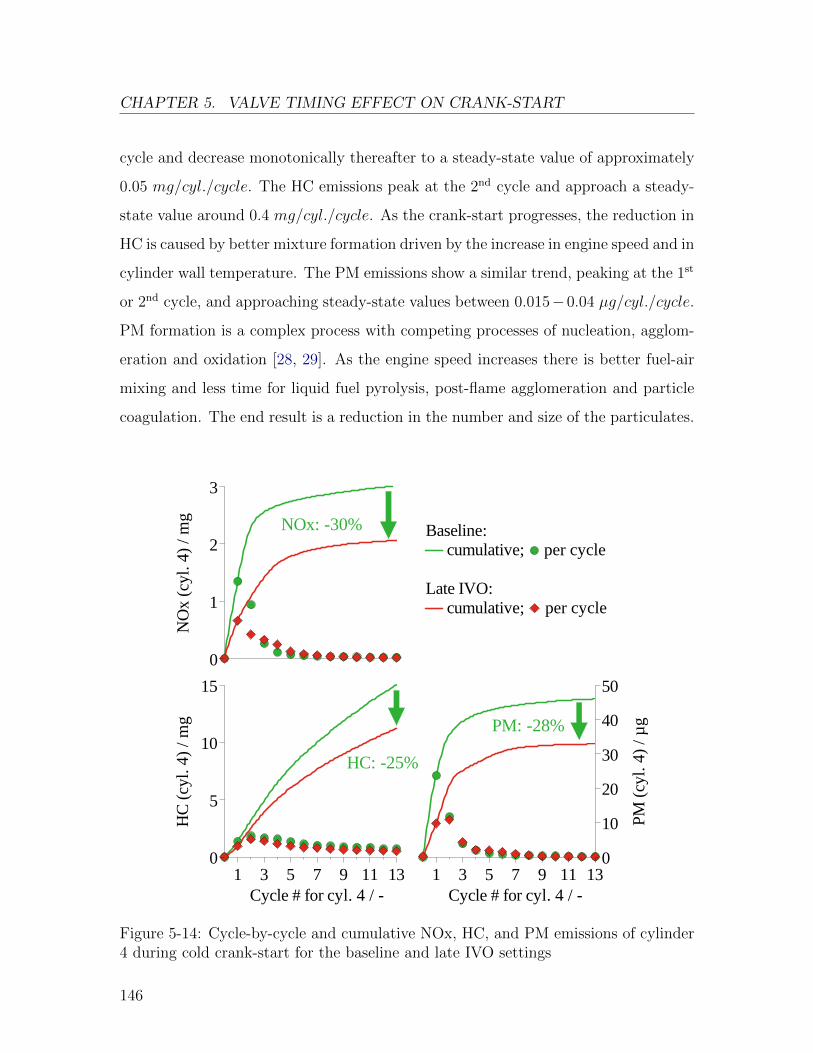
CHAPTER 5. VALVE TIMING EFFECT ON CRANK-START
cycle and decrease monotonically thereafter to a steady-state value of approximately
0.05 mg/cyl./cycle. The HC emissions peak at the 2nd cycle and approach a steady-
state value around 0.4 mg/cyl./cycle. As the crank-start progresses, the reduction in
HC is caused by better mixture formation driven by the increase in engine speed and in
cylinder wall temperature. The PM emissions show a similar trend, peaking at the 1st
or 2nd cycle, and approaching steady-state values between 0.015−0.04 µg/cyl./cycle.
PM formation is a complex process with competing processes of nucleation, agglom-
eration and oxidation [28, 29]. As the engine speed increases there is better fuel-air
mixing and less time for liquid fuel pyrolysis, post-flame agglomeration and particle
coagulation. The end result is a reduction in the number and size of the particulates.
Baseline: cumulative; per cycle
Late IVO: cumulative; per cycle
HC
(cy
l. 4
) /
mg
0
5
10
15
Cycle # for cyl. 4 / -1 3 5 7 9 11 13
HC: -25%
PM
(cy
l. 4)
/ µ
g
0
10
20
30
40
50
Cycle # for cyl. 4 / -1 3 5 7 9 11 13
PM: -28%
NO
x (c
yl. 4
) /
mg
0
1
2
3
NOx: -30%
Figure 5-14: Cycle-by-cycle and cumulative NOx, HC, and PM emissions of cylinder4 during cold crank-start for the baseline and late IVO settings
146
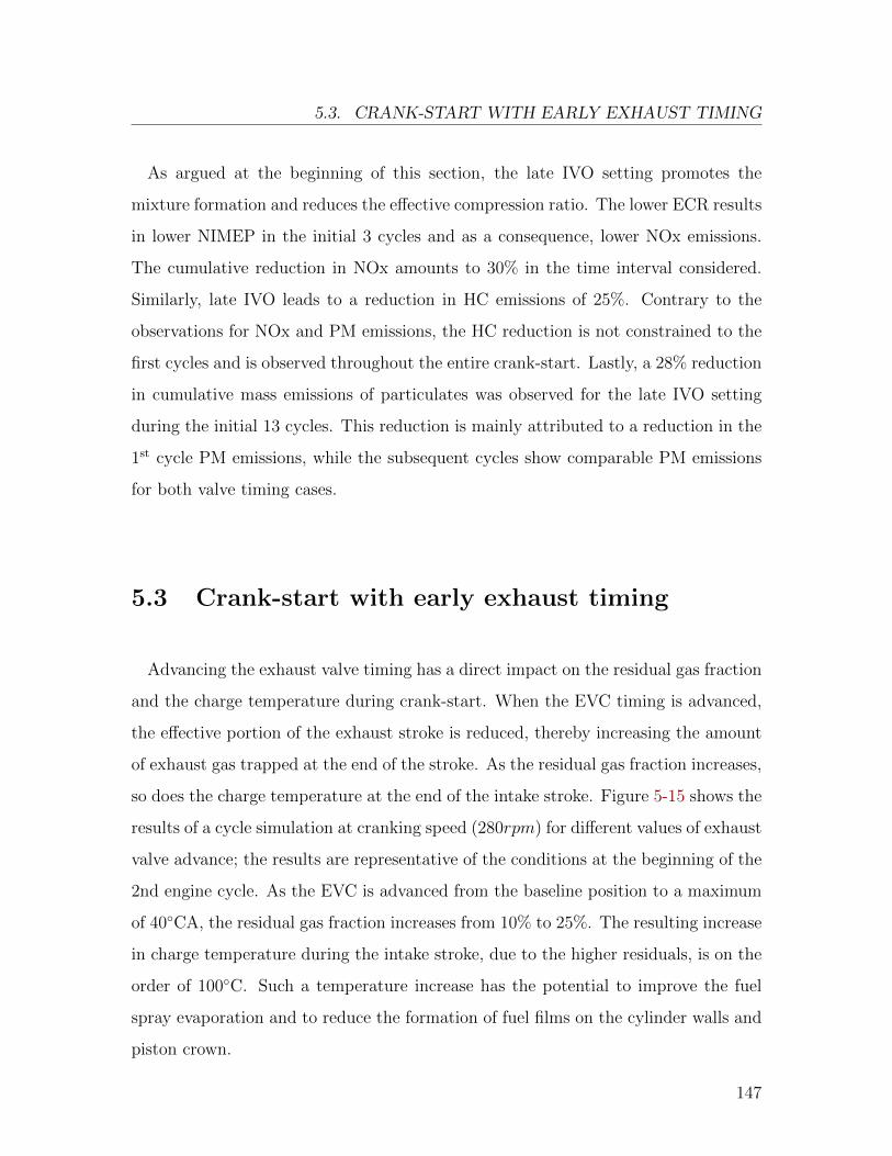
5.3. CRANK-START WITH EARLY EXHAUST TIMING
As argued at the beginning of this section, the late IVO setting promotes the
mixture formation and reduces the effective compression ratio. The lower ECR results
in lower NIMEP in the initial 3 cycles and as a consequence, lower NOx emissions.
The cumulative reduction in NOx amounts to 30% in the time interval considered.
Similarly, late IVO leads to a reduction in HC emissions of 25%. Contrary to the
observations for NOx and PM emissions, the HC reduction is not constrained to the
first cycles and is observed throughout the entire crank-start. Lastly, a 28% reduction
in cumulative mass emissions of particulates was observed for the late IVO setting
during the initial 13 cycles. This reduction is mainly attributed to a reduction in the
1st cycle PM emissions, while the subsequent cycles show comparable PM emissions
for both valve timing cases.
5.3 Crank-start with early exhaust timing
Advancing the exhaust valve timing has a direct impact on the residual gas fraction
and the charge temperature during crank-start. When the EVC timing is advanced,
the effective portion of the exhaust stroke is reduced, thereby increasing the amount
of exhaust gas trapped at the end of the stroke. As the residual gas fraction increases,
so does the charge temperature at the end of the intake stroke. Figure 5-15 shows the
results of a cycle simulation at cranking speed (280rpm) for different values of exhaust
valve advance; the results are representative of the conditions at the beginning of the
2nd engine cycle. As the EVC is advanced from the baseline position to a maximum
of 40◦CA, the residual gas fraction increases from 10% to 25%. The resulting increase
in charge temperature during the intake stroke, due to the higher residuals, is on the
order of 100◦C. Such a temperature increase has the potential to improve the fuel
spray evaporation and to reduce the formation of fuel films on the cylinder walls and
piston crown.
147
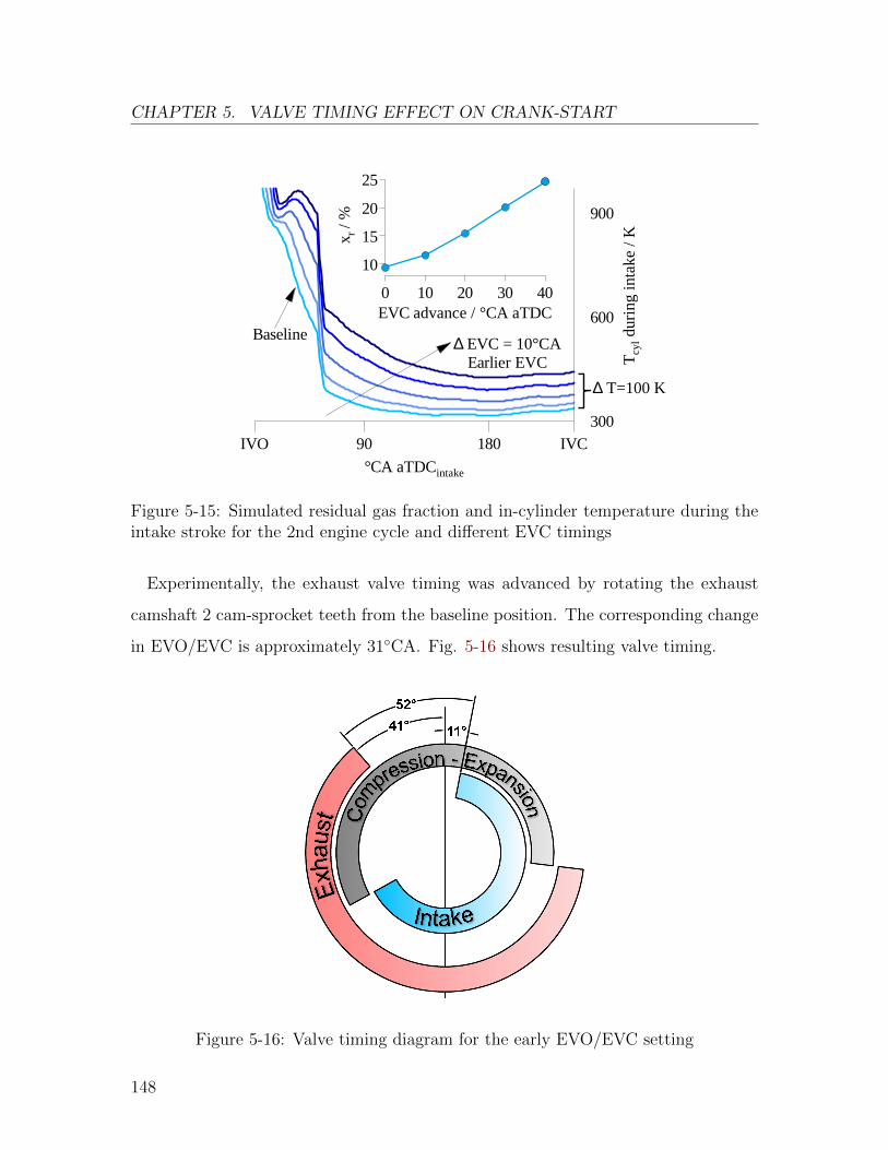
CHAPTER 5. VALVE TIMING EFFECT ON CRANK-START
∆ T=100 K T
cyl d
urin
g in
take
/ K
300
600
900
°CA aTDCintake
90 180IVO IVC
∆ EVC = 10°CAEarlier EVC
BaselineEVC advance / °CA aTDC0 10 20 30 40
x r /
%
10
15
20
25
Figure 5-15: Simulated residual gas fraction and in-cylinder temperature during theintake stroke for the 2nd engine cycle and different EVC timings
Experimentally, the exhaust valve timing was advanced by rotating the exhaust
camshaft 2 cam-sprocket teeth from the baseline position. The corresponding change
in EVO/EVC is approximately 31◦CA. Fig. 5-16 shows resulting valve timing.
Figure 5-16: Valve timing diagram for the early EVO/EVC setting
148
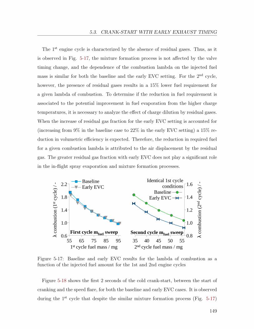
5.3. CRANK-START WITH EARLY EXHAUST TIMING
The 1st engine cycle is characterized by the absence of residual gases. Thus, as it
is observed in Fig. 5-17, the mixture formation process is not affected by the valve
timing change, and the dependence of the combustion lambda on the injected fuel
mass is similar for both the baseline and the early EVC setting. For the 2nd cycle,
however, the presence of residual gases results in a 15% lower fuel requirement for
a given lambda of combustion. To determine if the reduction in fuel requirement is
associated to the potential improvement in fuel evaporation from the higher charge
temperatures, it is necessary to analyze the effect of charge dilution by residual gases.
When the increase of residual gas fraction for the early EVC setting is accounted for
(increasing from 9% in the baseline case to 22% in the early EVC setting) a 15% re-
duction in volumetric efficiency is expected. Therefore, the reduction in required fuel
for a given combustion lambda is attributed to the air displacement by the residual
gas. The greater residual gas fraction with early EVC does not play a significant role
in the in-flight spray evaporation and mixture formation processes.
λ co
mbu
stio
n (1
st c
ycle
) / -
0.6
1.0
1.4
1.8
2.2
1st cycle fuel mass / mg55 65 75 85 95
Baseline Early EVC
First cycle mfuel sweep
λ co
mbu
stio
n (2
nd c
ycle
) / -
0.8
1.0
1.2
1.4
1.6
2nd cycle fuel mass / mg35 40 45 50 55
Identical 1st cycleconditions
Baseline Early EVC
Second cycle mfuel sweep
Figure 5-17: Baseline and early EVC results for the lambda of combustion as afunction of the injected fuel amount for the 1st and 2nd engine cycles
Figure 5-18 shows the first 2 seconds of the cold crank-start, between the start of
cranking and the speed flare, for both the baseline and early EVC cases. It is observed
during the 1st cycle that despite the similar mixture formation process (Fig. 5-17)
149
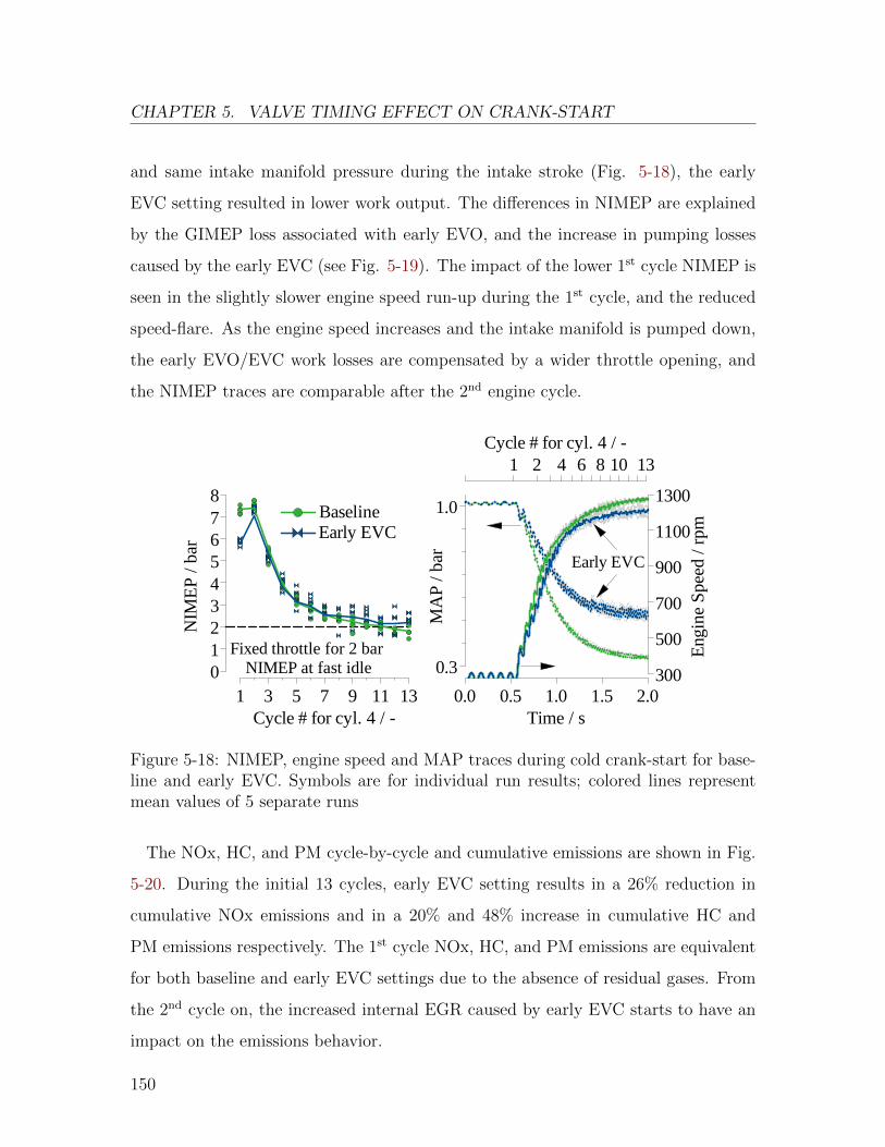
CHAPTER 5. VALVE TIMING EFFECT ON CRANK-START
and same intake manifold pressure during the intake stroke (Fig. 5-18), the early
EVC setting resulted in lower work output. The differences in NIMEP are explained
by the GIMEP loss associated with early EVO, and the increase in pumping losses
caused by the early EVC (see Fig. 5-19). The impact of the lower 1st cycle NIMEP is
seen in the slightly slower engine speed run-up during the 1st cycle, and the reduced
speed-flare. As the engine speed increases and the intake manifold is pumped down,
the early EVO/EVC work losses are compensated by a wider throttle opening, and
the NIMEP traces are comparable after the 2nd engine cycle.
MA
P / b
ar
0.3
1.0
Time / s0.0 0.5 1.0 1.5 2.0
Early EVC
NIM
EP
/ ba
r
012345678
Cycle # for cyl. 4 / -1 3 5 7 9 11 13
Baseline Early EVC
Fixed throttle for 2 bar NIMEP at fast idle
Eng
ine
Spe
ed /
rpm
300
500
700
900
1100
1300
Cycle # for cyl. 4 / -1 2 4 6 8 10 13
Figure 5-18: NIMEP, engine speed and MAP traces during cold crank-start for base-line and early EVC. Symbols are for individual run results; colored lines representmean values of 5 separate runs
The NOx, HC, and PM cycle-by-cycle and cumulative emissions are shown in Fig.
5-20. During the initial 13 cycles, early EVC setting results in a 26% reduction in
cumulative NOx emissions and in a 20% and 48% increase in cumulative HC and
PM emissions respectively. The 1st cycle NOx, HC, and PM emissions are equivalent
for both baseline and early EVC settings due to the absence of residual gases. From
the 2nd cycle on, the increased internal EGR caused by early EVC starts to have an
impact on the emissions behavior.
150
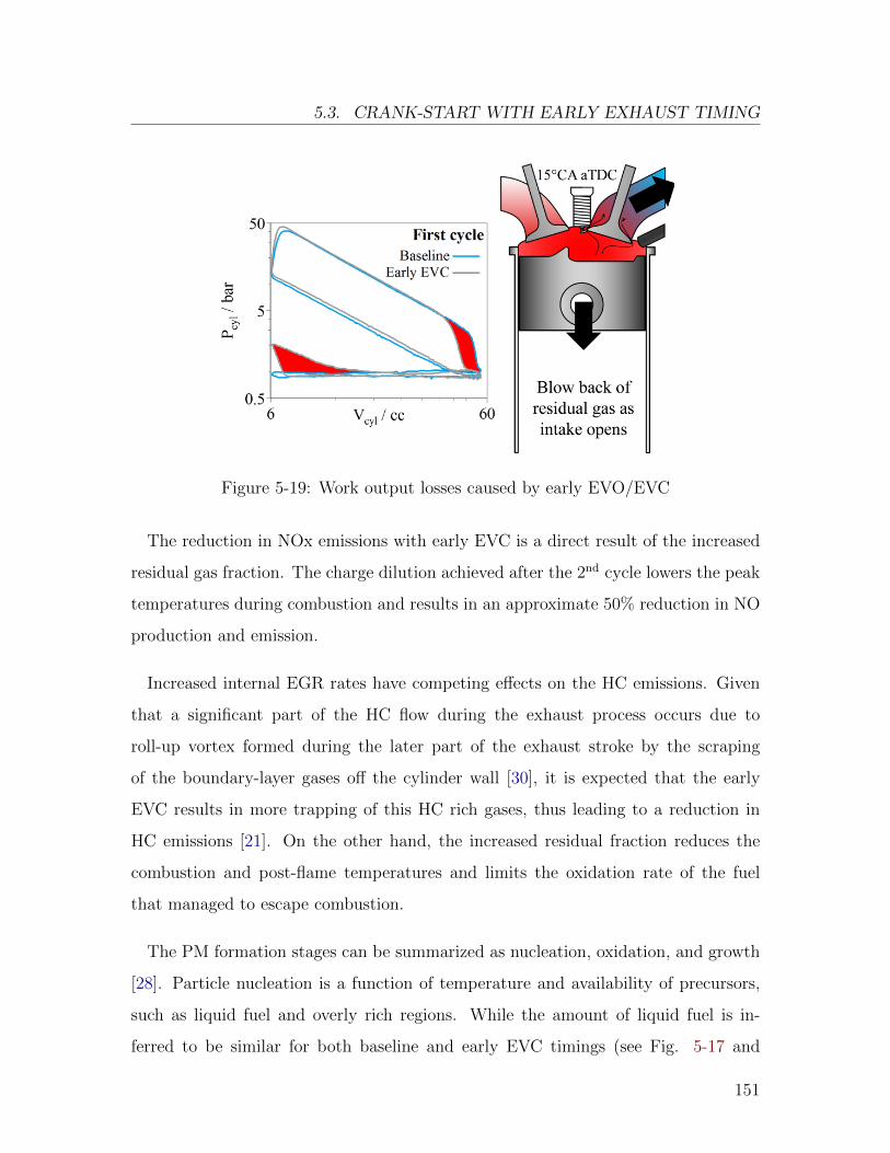
5.3. CRANK-START WITH EARLY EXHAUST TIMING
Figure 5-19: Work output losses caused by early EVO/EVC
The reduction in NOx emissions with early EVC is a direct result of the increased
residual gas fraction. The charge dilution achieved after the 2nd cycle lowers the peak
temperatures during combustion and results in an approximate 50% reduction in NO
production and emission.
Increased internal EGR rates have competing effects on the HC emissions. Given
that a significant part of the HC flow during the exhaust process occurs due to
roll-up vortex formed during the later part of the exhaust stroke by the scraping
of the boundary-layer gases off the cylinder wall [30], it is expected that the early
EVC results in more trapping of this HC rich gases, thus leading to a reduction in
HC emissions [21]. On the other hand, the increased residual fraction reduces the
combustion and post-flame temperatures and limits the oxidation rate of the fuel
that managed to escape combustion.
The PM formation stages can be summarized as nucleation, oxidation, and growth
[28]. Particle nucleation is a function of temperature and availability of precursors,
such as liquid fuel and overly rich regions. While the amount of liquid fuel is in-
ferred to be similar for both baseline and early EVC timings (see Fig. 5-17 and
151
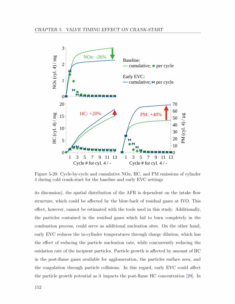
CHAPTER 5. VALVE TIMING EFFECT ON CRANK-START
Baseline: cumulative; per cycle
Early EVC: cumulative; per cycle
PM: +48%HC: +20%
NOx: -26%H
C (
cyl.
4)
/ m
g
0
5
10
15
20
Cycle # for cyl. 4 / -1 3 5 7 9 11 13
PM
(cy
l. 4)
/ µ
g
0
10
20
30
40
50
60
70
Cycle # for cyl. 4 / -1 3 5 7 9 11 13
NO
x (c
yl. 4
) /
mg
0
1
2
3
Figure 5-20: Cycle-by-cycle and cumulative NOx, HC, and PM emissions of cylinder4 during cold crank-start for the baseline and early EVC settings
its discussion), the spatial distribution of the AFR is dependent on the intake flow
structure, which could be affected by the blow-back of residual gases at IVO. This
effect, however, cannot be estimated with the tools used in this study. Additionally,
the particles contained in the residual gases which fail to burn completely in the
combustion process, could serve as additional nucleation sites. On the other hand,
early EVC reduces the in-cylinder temperatures through charge dilution, which has
the effect of reducing the particle nucleation rate, while concurrently reducing the
oxidation rate of the incipient particles. Particle growth is affected by amount of HC
in the post-flame gases available for agglomeration, the particles surface area, and
the coagulation through particle collisions. In this regard, early EVC could affect
the particle growth potential as it impacts the post-flame HC concentration [29]. In
152
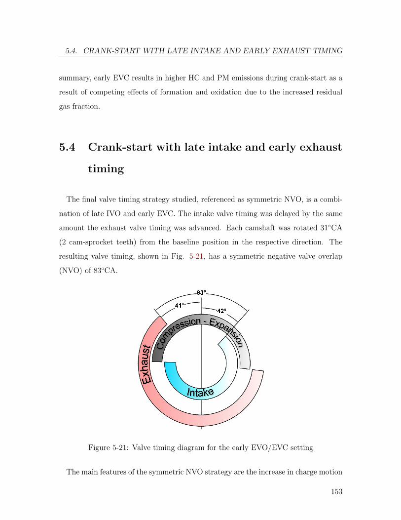
5.4. CRANK-START WITH LATE INTAKE AND EARLY EXHAUST TIMING
summary, early EVC results in higher HC and PM emissions during crank-start as a
result of competing effects of formation and oxidation due to the increased residual
gas fraction.
5.4 Crank-start with late intake and early exhaust
timing
The final valve timing strategy studied, referenced as symmetric NVO, is a combi-
nation of late IVO and early EVC. The intake valve timing was delayed by the same
amount the exhaust valve timing was advanced. Each camshaft was rotated 31◦CA
(2 cam-sprocket teeth) from the baseline position in the respective direction. The
resulting valve timing, shown in Fig. 5-21, has a symmetric negative valve overlap
(NVO) of 83◦CA.
Figure 5-21: Valve timing diagram for the early EVO/EVC setting
The main features of the symmetric NVO strategy are the increase in charge motion
153
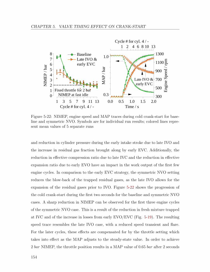
CHAPTER 5. VALVE TIMING EFFECT ON CRANK-START
MA
P / b
ar
0.3
1.0
Time / s0.0 0.5 1.0 1.5 2.0
Late IVO & early EVCN
IME
P /
bar
012345678
Cycle # for cyl. 4 / -1 3 5 7 9 11 13
Baseline Late IVO &
early EVC
Fixed throttle for 2 bar NIMEP at fast idle
Eng
ine
Spe
ed /
rpm
300
500
700
900
1100
1300
Cycle # for cyl. 4 / -1 2 4 6 8 10 13
Figure 5-22: NIMEP, engine speed and MAP traces during cold crank-start for base-line and symmetric NVO. Symbols are for individual run results; colored lines repre-sent mean values of 5 separate runs
and reduction in cylinder pressure during the early intake stroke due to late IVO and
the increase in residual gas fraction brought along by early EVC. Additionally, the
reduction in effective compression ratio due to late IVC and the reduction in effective
expansion ratio due to early EVO have an impact in the work output of the first few
engine cycles. In comparison to the early EVC strategy, the symmetric NVO setting
reduces the blow-back of the trapped residual gases, as the late IVO allows for the
expansion of the residual gases prior to IVO. Figure 5-22 shows the progression of
the cold crank-start during the first two seconds for the baseline and symmetric NVO
cases. A sharp reduction in NIMEP can be observed for the first three engine cycles
of the symmetric NVO case. This is a result of the reduction in fresh mixture trapped
at IVC and of the increase in losses from early EVO/EVC (Fig. 5-19). The resulting
speed trace resembles the late IVO case, with a reduced speed transient and flare.
For the later cycles, these effects are compensated for by the throttle setting which
takes into effect as the MAP adjusts to the steady-state value. In order to achieve
2 bar NIMEP, the throttle position results in a MAP value of 0.65 bar after 2 seconds
154
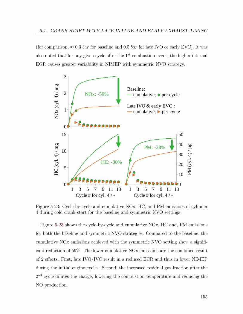
5.4. CRANK-START WITH LATE INTAKE AND EARLY EXHAUST TIMING
(for comparison, ≈ 0.3 bar for baseline and 0.5 bar for late IVO or early EVC). It was
also noted that for any given cycle after the 1st combustion event, the higher internal
EGR causes greater variability in NIMEP with symmetric NVO strategy.
HC
(cy
l. 4
) /
mg
0
5
10
15
Cycle # for cyl. 4 / -1 3 5 7 9 11 13
Baseline: cumulative; per cycle
Late IVO & early EVC : cumulative; per cycle
HC: -30%
PM
(cy
l. 4)
/ µ
g0
10
20
30
40
50
Cycle # for cyl. 4 / -1 3 5 7 9 11 13
PM: -28%
NO
x (c
yl. 4
) /
mg
0
1
2
3
NOx: -59%
Figure 5-23: Cycle-by-cycle and cumulative NOx, HC, and PM emissions of cylinder4 during cold crank-start for the baseline and symmetric NVO settings
Figure 5-23 shows the cycle-by-cycle and cumulative NOx, HC and, PM emissions
for both the baseline and symmetric NVO strategies. Compared to the baseline, the
cumulative NOx emissions achieved with the symmetric NVO setting show a signifi-
cant reduction of 59%. The lower cumulative NOx emissions are the combined result
of 2 effects. First, late IVO/IVC result in a reduced ECR and thus in lower NIMEP
during the initial engine cycles. Second, the increased residual gas fraction after the
2nd cycle dilutes the charge, lowering the combustion temperature and reducing the
NO production.
155
CHAPTER 5. VALVE TIMING EFFECT ON CRANK-START
Comparing the symmetric NVO to the previous two strategies discussed (late IVO:
Fig. 5-14; early EVC: Fig. 5-20), the measurements show a greater resemblance to
the HC and PM emissions reduction achieved with late IVO, as they are reduced in
30% and 28% correspondingly with respect to the baseline. The reduction in HC
emissions is more prominent during the initial five engine cycles, with the difference
becoming smaller as the crank-start progresses. As in the late IVO case, the reduction
in PM stems mainly from the 1st cycle.
Late IVO alone was advantageous in the mixture formation process, improving
spray evaporation and reducing the amount of fuel films serving as HC and PM
sources. Additionally, the lower volumetric efficiency caused by the late IVC event,
reduces the total mass exhausted during the critical 1st cycle, for which the intake
pressure is close to atmospheric. Conversely, the early EVC results described in the
previous section showed an increase in HC and PM emissions, due to the unbalance
of the competing effects of increased internal EGR on the HC and PM formation
and oxidation. From a simplified analysis, the emissions behavior of the combined
strategy was expected to fall between the two cases previously described. However,
the combined effect of late IVO and early EVC on the temporal and spatial evolution
of the inlet flow, AFR, EGR, charge temperature and fuel films cannot be assessed
with the experimental capabilities of this study and no further explanation can be
provided for the observed trends.
5.5 Findings
The effects of four valve timing settings on the cold-start NOx, HC and PM emis-
sions during crank-start were studied in a wall guided gasoline direct injection engine.
The valve timings examined were the stock position, late IVO, early EVC and a com-
bination of the latter, dubbed symmetric NVO. The following conclusions are drawn:
156
5.5. FINDINGS
� Late IVO improves the mixture formation process in cold crank-start and re-
duces the exhaust mass flow during the critical 1st cycle exhaust event. The
delayed intake timing results in 25% and 28% reduction of the cumulative HC
and PM cold crank-start emissions respectively. During the initial cycles, late
IVC results in lower NIMEP and in-cylinder temperatures reducing the rate of
NO formation.
� The effect of early EVC timing on the crank-start emissions is due to the increase
in residual gas fraction. For this reason it does not have any effect on the 1st
cycle. Early EVC results in an improvement in NOx emissions after the 2nd
engine cycle and in a deterioration of the HC and PM/PN emissions in cold
crank-start. The increase in cumulative HC and PM emissions comprises mainly
the contributions from the early cycles (2nd through 5th).
� The combined strategy consisting of late intake and early exhaust phasing shows
a significant reduction in the cumulative crank-start NOx emissions due to the
combination of increased residuals and lower NIMEP of the initial cycles. Fur-
thermore, the reduction in cumulative HC and PM/PN emissions is similar in
magnitude and cycle-to-cycle progression to the late IVO case. Thus early EVC
has less impact on the crank-start HC and PM emissions compared to late IVO.
157

– Intentionally left blank –
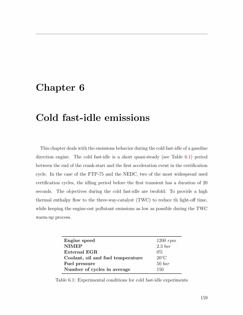
Chapter 6
Cold fast-idle emissions
This chapter deals with the emissions behavior during the cold fast-idle of a gasoline
direction engine. The cold fast-idle is a short quasi-steady (see Table 6.1) period
between the end of the crank-start and the first acceleration event in the certification
cycle. In the case of the FTP-75 and the NEDC, two of the most widespread used
certification cycles, the idling period before the first transient has a duration of 20
seconds. The objectives during the cold fast-idle are twofold: To provide a high
thermal enthalpy flow to the three-way-catalyst (TWC) to reduce th light-off time,
while keeping the engine-out pollutant emissions as low as possible during the TWC
warm-up process.
Engine speed 1200 rpmNIMEP 2.3 barExternal EGR 0%Coolant, oil and fuel temperature 20◦CFuel pressure 50 barNumber of cycles in average 150
Table 6.1: Experimental conditions for cold fast-idle experiments
159
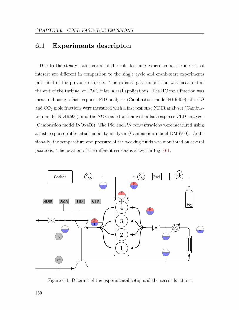
CHAPTER 6. COLD FAST-IDLE EMISSIONS
6.1 Experiments descripton
Due to the steady-state nature of the cold fast-idle experiments, the metrics of
interest are different in comparison to the single cycle and crank-start experiments
presented in the previous chapters. The exhaust gas composition was measured at
the exit of the turbine, or TWC inlet in real applications. The HC mole fraction was
measured using a fast response FID analyzer (Cambustion model HFR400), the CO
and CO2 mole fractions were measured with a fast response NDIR analyzer (Cambus-
tion model NDIR500), and the NOx mole fraction with a fast response CLD analyzer
(Cambustion model fNOx400). The PM and PN concentrations were measured using
a fast response differential mobolity analyzer (Cambustion model DMS500). Addi-
tionally, the temperature and pressure of the working fluids was monitored on several
positions. The location of the different sensors is shown in Fig. 6-1.
4
3
2
1
N2
FuelCoolant
λ
m
PT
T
T
T
P
TP
T
CLDFIDDMANDIR
TP
T
Figure 6-1: Diagram of the experimental setup and the sensor locations
160
6.2. AIR-FUEL EQUIVALENCE RATIO
Previous work at MIT has focused on extensively characterizing the cold fast-idle
emissions of HC [9] and particulates [36]. The experiments presented in this chapter
seek to expand the previous analysis to include NOx emissions and unconventional
valve timing. The variables studied and object of the following sections are:
1. Air-fuel equivalence ratio
2. Split-injection strategies
3. Combustion phasing
4. Valve timing
6.2 Air-fuel equivalence ratio
During the normal operation of stoichiometric gasoline engines, the air-fuel equiv-
alence ratio is carefully regulated around λ = 1 to ensure that the TWC catalyst
mantains a certain level of oxygen storage so that it can effectively oxide HC and
CO emissions to CO2 and reduce NOx emissions to N2. However, during cold fast-
idle, this constrain is lifted due to the catalytic inactivity of the TWC. This section
presents the effect of lambda on the engine out emissions, exhaust enthalpy and en-
gine stability. Table 6.2 presents the specific details of the air-fuel equivalence ratio
experiments, in addition to the operating conditions presented in Table 6.1.
Spark timing 5◦CA aTDCcomp.
Start of Injection 105◦CA aTDCintake
Injection pulse duration 1520 µsInjected mass 17.1 mgValve timing Baseline (Table 5.1)
Table 6.2: Injection strategy for lambda sweep
161
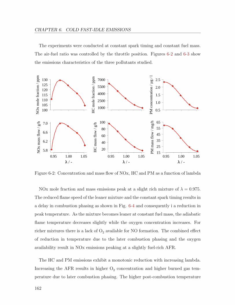
CHAPTER 6. COLD FAST-IDLE EMISSIONS
The experiments were conducted at constant spark timing and constant fuel mass.
The air-fuel ratio was controlled by the throttle position. Figures 6-2 and 6-3 show
the emissions characteristics of the three pollutants studied.
HC
mo
le fr
actio
n /
ppm
1000
2500
4000
5500
7000
HC
mas
s flo
w /
g/h
20
40
60
80
100
λ / -0.95 1.00 1.05
PM
mas
s flo
w /
mg/
h15
25
35
45
55
65
λ / -0.95 1.00 1.05
NO
x m
ole
frac
tion
/ pp
m
100105110115120125130
NO
x m
ass
flow
/ g
/h
5.8
6.2
6.6
7.0
λ / -0.95 1.00 1.05
PM
co
ncen
trat
ion
/ µ
g /
l
0.5
1.0
1.5
2.0
2.5
Figure 6-2: Concentration and mass flow of NOx, HC and PM as a function of lambda
NOx mole fraction and mass emissions peak at a slight rich mixture of λ = 0.975.
The reduced flame speed of the leaner mixture and the constant spark timing results in
a delay in combustion phasing as shown in Fig. 6-4 and consequently i a reduction in
peak temperature. As the mixture becomes leaner at constant fuel mass, the adiabatic
flame temperature decreases slightly while the oxygen concentration increases. For
richer mixtures there is a lack of O2 available for NO formation. The combined effect
of reduction in temperature due to the later combustion phasing and the oxygen
availability result in NOx emissions peaking at a slightly fuel-rich AFR.
The HC and PM emissions exhibit a monotonic reduction with increasing lambda.
Increasing the AFR results in higher O2 concentration and higher burned gas tem-
perature due to later combustion phasing. The higher post-combustion temperature
162
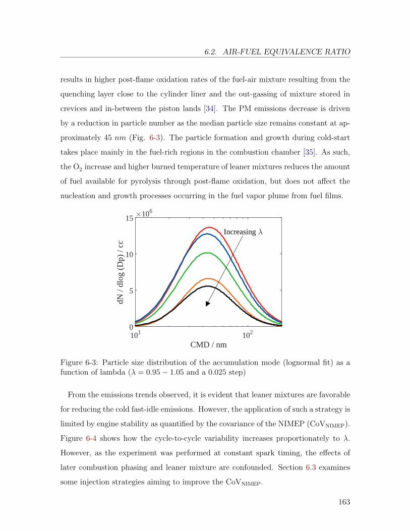
6.2. AIR-FUEL EQUIVALENCE RATIO
results in higher post-flame oxidation rates of the fuel-air mixture resulting from the
quenching layer close to the cylinder liner and the out-gassing of mixture stored in
crevices and in-between the piston lands [34]. The PM emissions decrease is driven
by a reduction in particle number as the median particle size remains constant at ap-
proximately 45 nm (Fig. 6-3). The particle formation and growth during cold-start
takes place mainly in the fuel-rich regions in the combustion chamber [35]. As such,
the O2 increase and higher burned temperature of leaner mixtures reduces the amount
of fuel available for pyrolysis through post-flame oxidation, but does not affect the
nucleation and growth processes occurring in the fuel vapor plume from fuel films.
CMD / nm101 102
dN /
dlog
(D
p) /
cc
×106
0
5
10
15
Increasing λ
Figure 6-3: Particle size distribution of the accumulation mode (lognormal fit) as afunction of lambda (λ = 0.95− 1.05 and a 0.025 step)
From the emissions trends observed, it is evident that leaner mixtures are favorable
for reducing the cold fast-idle emissions. However, the application of such a strategy is
limited by engine stability as quantified by the covariance of the NIMEP (CoVNIMEP).
Figure 6-4 shows how the cycle-to-cycle variability increases proportionately to λ.
However, as the experiment was performed at constant spark timing, the effects of
later combustion phasing and leaner mixture are confounded. Section 6.3 examines
some injection strategies aiming to improve the CoVNIMEP.
163
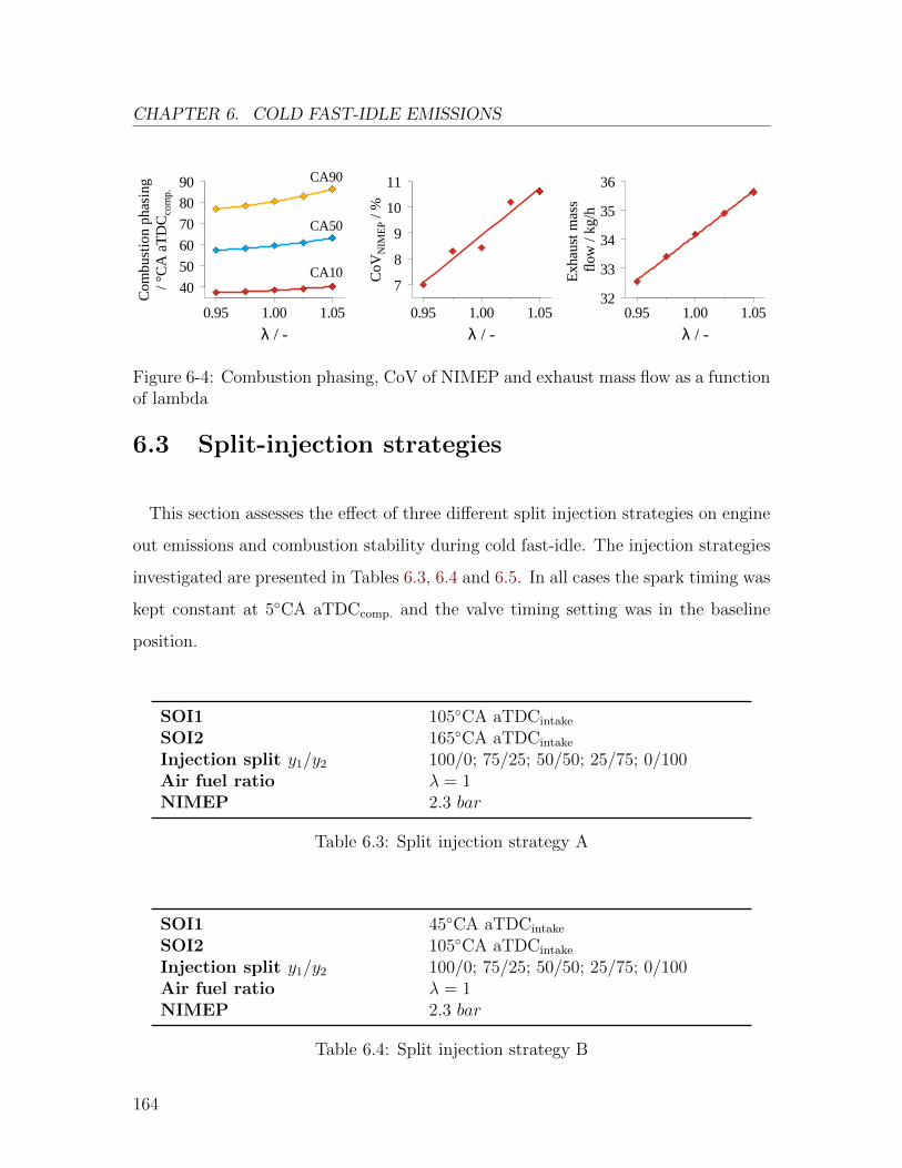
CHAPTER 6. COLD FAST-IDLE EMISSIONS
CoV
NIM
EP /
%
7
8
9
10
11
λ / -0.95 1.00 1.05
Exh
aust
mas
s flo
w /
kg/h
32
33
34
35
36
λ / -0.95 1.00 1.05
Com
bust
ion
pha
sing
/ °C
A a
TD
C com
p.
40
50
60
70
80
90
λ / -0.95 1.00 1.05
CA10
CA50
CA90
Figure 6-4: Combustion phasing, CoV of NIMEP and exhaust mass flow as a functionof lambda
6.3 Split-injection strategies
This section assesses the effect of three different split injection strategies on engine
out emissions and combustion stability during cold fast-idle. The injection strategies
investigated are presented in Tables 6.3, 6.4 and 6.5. In all cases the spark timing was
kept constant at 5◦CA aTDCcomp. and the valve timing setting was in the baseline
position.
SOI1 105◦CA aTDCintake
SOI2 165◦CA aTDCintake
Injection split y1/y2 100/0; 75/25; 50/50; 25/75; 0/100Air fuel ratio λ = 1NIMEP 2.3 bar
Table 6.3: Split injection strategy A
SOI1 45◦CA aTDCintake
SOI2 105◦CA aTDCintake
Injection split y1/y2 100/0; 75/25; 50/50; 25/75; 0/100Air fuel ratio λ = 1NIMEP 2.3 bar
Table 6.4: Split injection strategy B
164
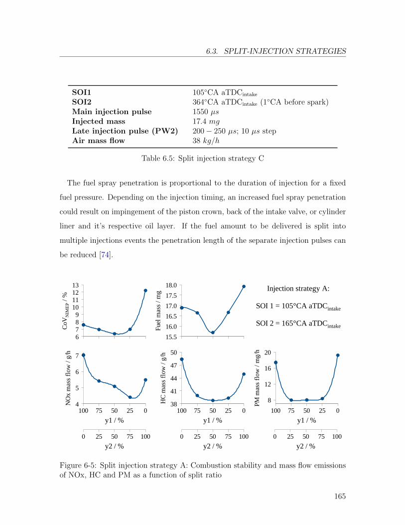
6.3. SPLIT-INJECTION STRATEGIES
SOI1 105◦CA aTDCintake
SOI2 364◦CA aTDCintake (1◦CA before spark)Main injection pulse 1550 µsInjected mass 17.4 mgLate injection pulse (PW2) 200− 250 µs; 10 µs stepAir mass flow 38 kg/h
Table 6.5: Split injection strategy C
The fuel spray penetration is proportional to the duration of injection for a fixed
fuel pressure. Depending on the injection timing, an increased fuel spray penetration
could result on impingement of the piston crown, back of the intake valve, or cylinder
liner and it’s respective oil layer. If the fuel amount to be delivered is split into
multiple injections events the penetration length of the separate injection pulses can
be reduced [74].
Injection strategy A:
SOI 1 = 105°CA aTDCintake
SOI 2 = 165°CA aTDCintake
HC
mas
s flo
w /
g/h
38
41
44
47
50
y1 / %0255075100
PM
mas
s flo
w /
mg/
h
8
12
16
20
y1 / %0255075100
NO
x m
ass
flow
/ g
/h
4
5
6
7
y1 / %0255075100
y2 / %0 25 50 75 100
y2 / %0 25 50 75 100
y2 / %0 25 50 75 100
CoV
NIM
EP /
%
6789
10111213
Fue
l mas
s /
mg
15.5
16.0
16.5
17.0
17.5
18.0
Figure 6-5: Split injection strategy A: Combustion stability and mass flow emissionsof NOx, HC and PM as a function of split ratio
165
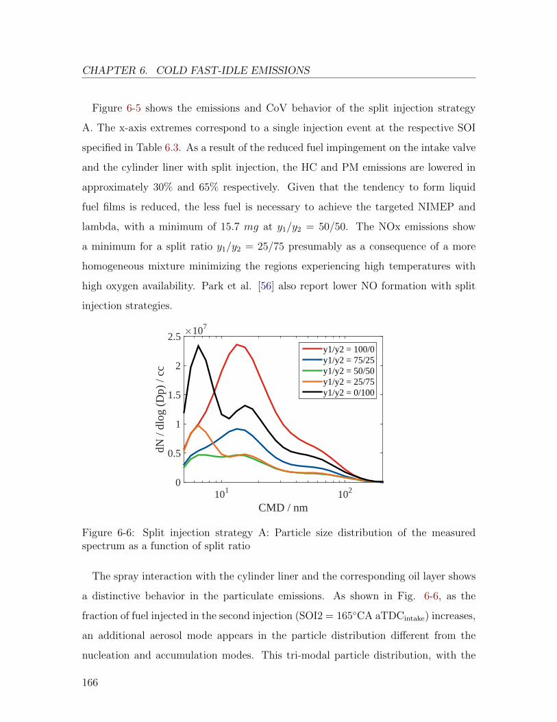
CHAPTER 6. COLD FAST-IDLE EMISSIONS
Figure 6-5 shows the emissions and CoV behavior of the split injection strategy
A. The x-axis extremes correspond to a single injection event at the respective SOI
specified in Table 6.3. As a result of the reduced fuel impingement on the intake valve
and the cylinder liner with split injection, the HC and PM emissions are lowered in
approximately 30% and 65% respectively. Given that the tendency to form liquid
fuel films is reduced, the less fuel is necessary to achieve the targeted NIMEP and
lambda, with a minimum of 15.7 mg at y1/y2 = 50/50. The NOx emissions show
a minimum for a split ratio y1/y2 = 25/75 presumably as a consequence of a more
homogeneous mixture minimizing the regions experiencing high temperatures with
high oxygen availability. Park et al. [56] also report lower NO formation with split
injection strategies.
CMD / nm101 102
dN /
dlog
(D
p) /
cc
×107
0
0.5
1
1.5
2
2.5y1/y2 = 100/0y1/y2 = 75/25y1/y2 = 50/50y1/y2 = 25/75y1/y2 = 0/100
Figure 6-6: Split injection strategy A: Particle size distribution of the measuredspectrum as a function of split ratio
The spray interaction with the cylinder liner and the corresponding oil layer shows
a distinctive behavior in the particulate emissions. As shown in Fig. 6-6, as the
fraction of fuel injected in the second injection (SOI2 = 165◦CA aTDCintake) increases,
an additional aerosol mode appears in the particle distribution different from the
nucleation and accumulation modes. This tri-modal particle distribution, with the
166
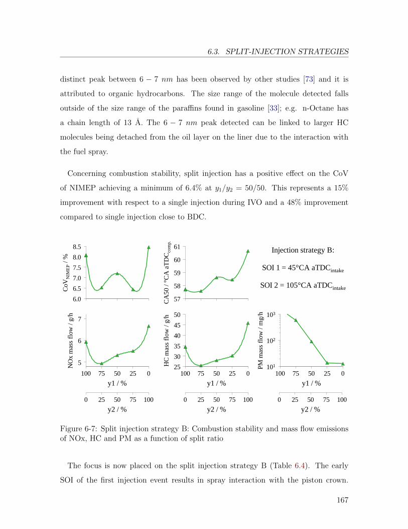
6.3. SPLIT-INJECTION STRATEGIES
distinct peak between 6 − 7 nm has been observed by other studies [73] and it is
attributed to organic hydrocarbons. The size range of the molecule detected falls
outside of the size range of the paraffins found in gasoline [33]; e.g. n-Octane has
a chain length of 13 A. The 6 − 7 nm peak detected can be linked to larger HC
molecules being detached from the oil layer on the liner due to the interaction with
the fuel spray.
Concerning combustion stability, split injection has a positive effect on the CoV
of NIMEP achieving a minimum of 6.4% at y1/y2 = 50/50. This represents a 15%
improvement with respect to a single injection during IVO and a 48% improvement
compared to single injection close to BDC.
Injection strategy B:
SOI 1 = 45°CA aTDCintake
SOI 2 = 105°CA aTDCintake
HC
mas
s flo
w /
g/h
25
30
35
40
45
50
y1 / %0255075100
PM
mas
s flo
w /
mg/
h
101
102
103
y1 / %0255075100
NO
x m
ass
flow
/ g
/h
5
6
7
y1 / %0255075100
y2 / %0 25 50 75 100
y2 / %0 25 50 75 100
y2 / %0 25 50 75 100
CoV
NIM
EP /
%
6.0
6.5
7.0
7.5
8.0
8.5
CA
50
/ °C
A a
TD
C com
p.
57
58
59
60
61
Figure 6-7: Split injection strategy B: Combustion stability and mass flow emissionsof NOx, HC and PM as a function of split ratio
The focus is now placed on the split injection strategy B (Table 6.4). The early
SOI of the first injection event results in spray interaction with the piston crown.
167
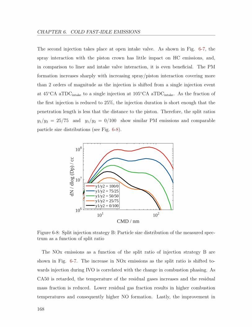
CHAPTER 6. COLD FAST-IDLE EMISSIONS
The second injection takes place at open intake valve. As shown in Fig. 6-7, the
spray interaction with the piston crown has little impact on HC emissions, and,
in comparison to liner and intake valve interaction, it is even beneficial. The PM
formation increases sharply with increasing spray/piston interaction covering more
than 2 orders of magnitude as the injection is shifted from a single injection event
at 45◦CA aTDCintake to a single injection at 105◦CA aTDCintake. As the fraction of
the first injection is reduced to 25%, the injection duration is short enough that the
penetration length is less that the distance to the piston. Therefore, the split ratios
y1/y2 = 25/75 and y1/y2 = 0/100 show similar PM emissions and comparable
particle size distributions (see Fig. 6-8).
CMD / nm101 102
dN /
dlog
(D
p) /
cc
106
107
108
y1/y2 = 100/0y1/y2 = 75/25y1/y2 = 50/50y1/y2 = 25/75y1/y2 = 0/100
Figure 6-8: Split injection strategy B: Particle size distribution of the measured spec-trum as a function of split ratio
The NOx emissions as a function of the split ratio of injection strategy B are
shown in Fig. 6-7. The increase in NOx emissions as the split ratio is shifted to-
wards injection during IVO is correlated with the change in combustion phasing. As
CA50 is retarded, the temperature of the residual gases increases and the residual
mass fraction is reduced. Lower residual gas fraction results in higher combustion
temperatures and consequently higher NO formation. Lastly, the improvement in
168
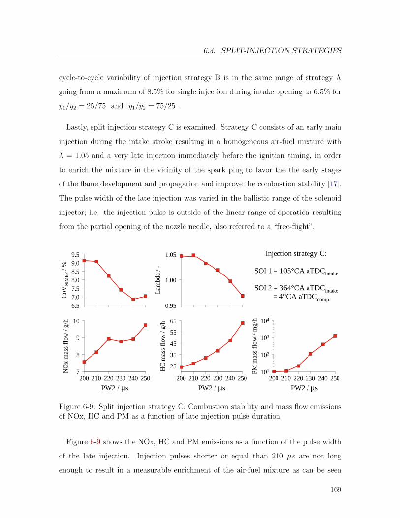
6.3. SPLIT-INJECTION STRATEGIES
cycle-to-cycle variability of injection strategy B is in the same range of strategy A
going from a maximum of 8.5% for single injection during intake opening to 6.5% for
y1/y2 = 25/75 and y1/y2 = 75/25 .
Lastly, split injection strategy C is examined. Strategy C consists of an early main
injection during the intake stroke resulting in a homogeneous air-fuel mixture with
λ = 1.05 and a very late injection immediately before the ignition timing, in order
to enrich the mixture in the vicinity of the spark plug to favor the the early stages
of the flame development and propagation and improve the combustion stability [17].
The pulse width of the late injection was varied in the ballistic range of the solenoid
injector; i.e. the injection pulse is outside of the linear range of operation resulting
from the partial opening of the nozzle needle, also referred to a “free-flight”.
Injection strategy C:
SOI 1 = 105°CA aTDCintake
SOI 2 = 364°CA aTDCintake = 4°CA aTDCcomp.
HC
mas
s flo
w /
g/h
25
35
45
55
65
PW2 / µs200 210 220 230 240 250
PM
mas
s flo
w /
mg/
h
101
102
103
104
PW2 / µs200 210 220 230 240 250
NO
x m
ass
flow
/ g
/h
7
8
9
10
PW2 / µs200 210 220 230 240 250
CoV
NIM
EP /
%
6.57.07.58.08.59.09.5
Lam
bda
/ -
0.95
1.00
1.05
Figure 6-9: Split injection strategy C: Combustion stability and mass flow emissionsof NOx, HC and PM as a function of late injection pulse duration
Figure 6-9 shows the NOx, HC and PM emissions as a function of the pulse width
of the late injection. Injection pulses shorter or equal than 210 µs are not long
enough to result in a measurable enrichment of the air-fuel mixture as can be seen
169
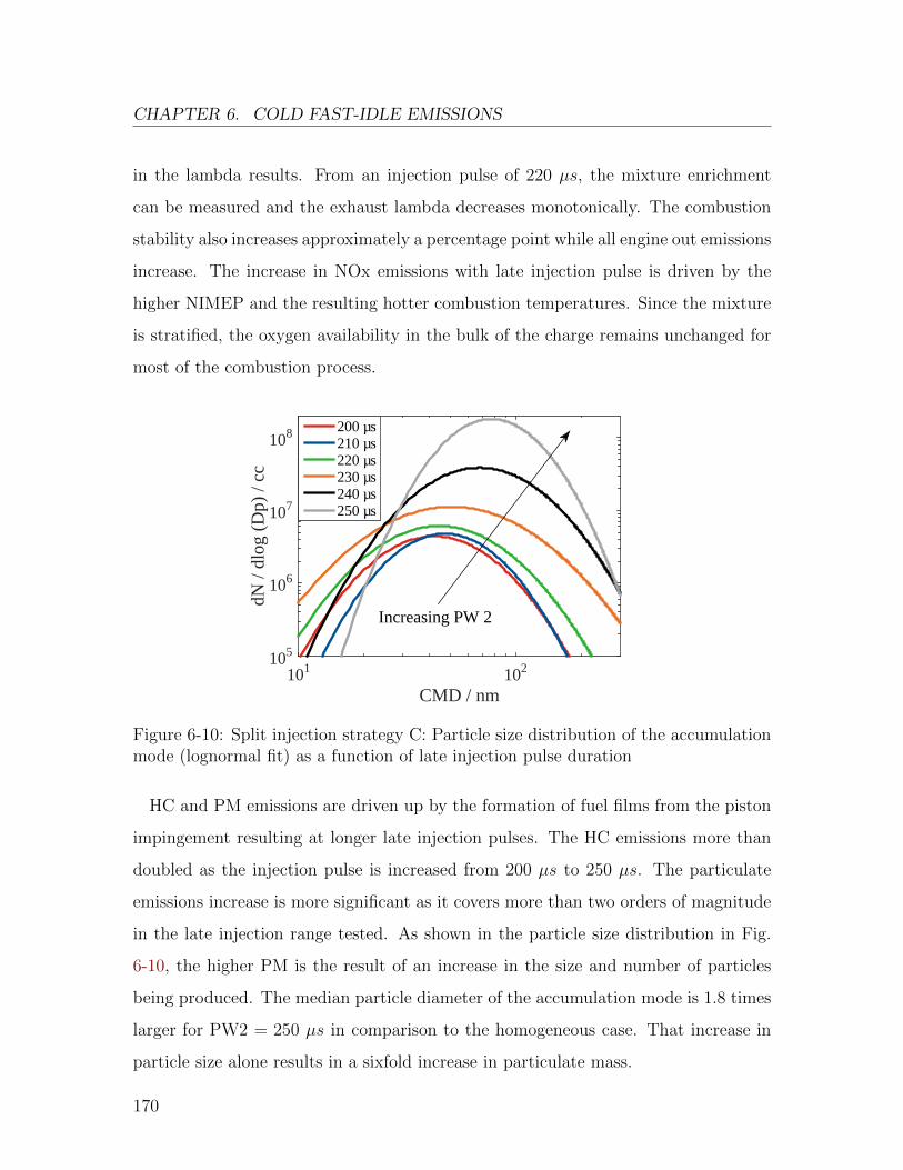
CHAPTER 6. COLD FAST-IDLE EMISSIONS
in the lambda results. From an injection pulse of 220 µs, the mixture enrichment
can be measured and the exhaust lambda decreases monotonically. The combustion
stability also increases approximately a percentage point while all engine out emissions
increase. The increase in NOx emissions with late injection pulse is driven by the
higher NIMEP and the resulting hotter combustion temperatures. Since the mixture
is stratified, the oxygen availability in the bulk of the charge remains unchanged for
most of the combustion process.
CMD / nm101 102
dN /
dlog
(D
p) /
cc
105
106
107
108 200 µs210 µs220 µs230 µs240 µs250 µs
Increasing PW 2
Figure 6-10: Split injection strategy C: Particle size distribution of the accumulationmode (lognormal fit) as a function of late injection pulse duration
HC and PM emissions are driven up by the formation of fuel films from the piston
impingement resulting at longer late injection pulses. The HC emissions more than
doubled as the injection pulse is increased from 200 µs to 250 µs. The particulate
emissions increase is more significant as it covers more than two orders of magnitude
in the late injection range tested. As shown in the particle size distribution in Fig.
6-10, the higher PM is the result of an increase in the size and number of particles
being produced. The median particle diameter of the accumulation mode is 1.8 times
larger for PW2 = 250 µs in comparison to the homogeneous case. That increase in
particle size alone results in a sixfold increase in particulate mass.
170
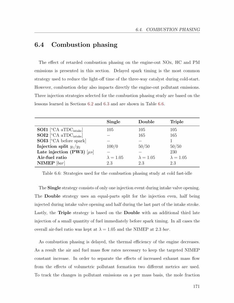
6.4. COMBUSTION PHASING
6.4 Combustion phasing
The effect of retarded combustion phasing on the engine-out NOx, HC and PM
emissions is presented in this section. Delayed spark timing is the most common
strategy used to reduce the light-off time of the three-way catalyst during cold-start.
However, combustion delay also impacts directly the engine-out pollutant emissions.
Three injection strategies selected for the combustion phasing study are based on the
lessons learned in Sections 6.2 and 6.3 and are shown in Table 6.6.
Single Double Triple
SOI1 [◦CA aTDCintake] 105 105 105SOI2 [◦CA aTDCintake] − 165 165SOI3 [◦CA before spark] − − 1Injection split y1/y2 100/0 50/50 50/50Late injection (PW3) [µs] − − 230Air-fuel ratio λ = 1.05 λ = 1.05 λ = 1.05NIMEP [bar] 2.3 2.3 2.3
Table 6.6: Strategies used for the combustion phasing study at cold fast-idle
The Single strategy consists of only one injection event during intake valve opening.
The Double strategy uses an equal-parts split for the injection even, half being
injected during intake valve opening and half during the last part of the intake stroke.
Lastly, the Triple strategy is based on the Double with an additional third late
injection of a small quantity of fuel immediately before spark timing. In all cases the
overall air-fuel ratio was kept at λ = 1.05 and the NIMEP at 2.3 bar.
As combustion phasing is delayed, the thermal efficiency of the engine decreases.
As a result the air and fuel mass flow rates necessary to keep the targeted NIMEP
constant increase. In order to separate the effects of increased exhaust mass flow
from the effects of volumetric pollutant formation two different metrics are used.
To track the changes in pollutant emissions on a per mass basis, the mole fraction
171
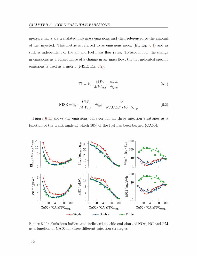
CHAPTER 6. COLD FAST-IDLE EMISSIONS
measurements are translated into mass emissions and then referenced to the amount
of fuel injected. This metric is referred to as emissions index (EI, Eq. 6.1) and as
such is independent of the air and fuel mass flow rates. To account for the change
in emissions as a consequence of a change in air mass flow, the net indicated specific
emissions is used as a metric (NISE, Eq. 6.2).
EI = xi ·MWi
MWexh
· mexh
mfuel
(6.1)
NISE = xi ·MWi
MWexh
· mexh ·2
NIMEP · Vd ·Neng
(6.2)
Figure 6-11 shows the emissions behavior for all three injection strategies as a
function of the crank angle at which 50% of the fuel has been burned (CA50).
Single Double Triple
EI H
C /
mg H
C /
g fue
l
0
10
20
30
40
isH
C /
g/kW
h
0
4
8
12
16
CA50 / °CA aTDCcomp.
0 20 40 60 80
isP
M /
mg
/kW
h
0.1
1
10
100
CA50 / °CA aTDCcomp.
0 20 40 60 80
EI P
M /
µg P
M /
g fue
l
1
10
100
1000
EI N
Ox
/ mg
NO
x / g
fuel
0
5
10
15
20
isN
Ox
/ g/k
Wh
0
2
4
6
CA50 / °CA aTDCcomp.
0 20 40 60 80
Figure 6-11: Emissions indices and indicated specific emissions of NOx, HC and PMas a function of CA50 for three different injection strategies
172
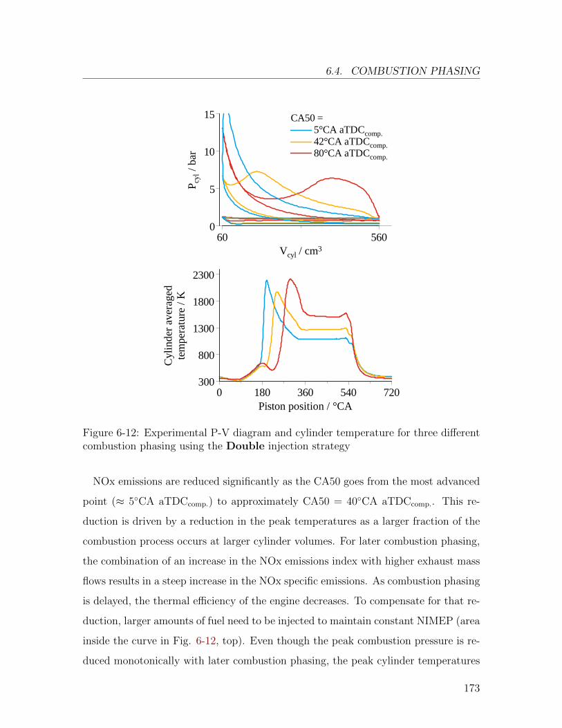
6.4. COMBUSTION PHASING
P cyl /
bar
0
5
10
15
Vcyl / cm360 560
Cyl
ind
er a
vera
ged
tem
pera
ture
/ K
300
800
1300
1800
2300
Piston position / °CA0 180 360 540 720
CA50 = 5°CA aTDCcomp. 42°CA aTDCcomp. 80°CA aTDCcomp.
Figure 6-12: Experimental P-V diagram and cylinder temperature for three differentcombustion phasing using the Double injection strategy
NOx emissions are reduced significantly as the CA50 goes from the most advanced
point (≈ 5◦CA aTDCcomp.) to approximately CA50 = 40◦CA aTDCcomp.. This re-
duction is driven by a reduction in the peak temperatures as a larger fraction of the
combustion process occurs at larger cylinder volumes. For later combustion phasing,
the combination of an increase in the NOx emissions index with higher exhaust mass
flows results in a steep increase in the NOx specific emissions. As combustion phasing
is delayed, the thermal efficiency of the engine decreases. To compensate for that re-
duction, larger amounts of fuel need to be injected to maintain constant NIMEP (area
inside the curve in Fig. 6-12, top). Even though the peak combustion pressure is re-
duced monotonically with later combustion phasing, the peak cylinder temperatures
173
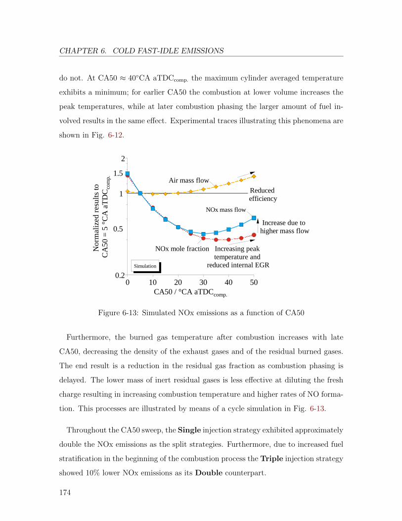
CHAPTER 6. COLD FAST-IDLE EMISSIONS
do not. At CA50 ≈ 40◦CA aTDCcomp. the maximum cylinder averaged temperature
exhibits a minimum; for earlier CA50 the combustion at lower volume increases the
peak temperatures, while at later combustion phasing the larger amount of fuel in-
volved results in the same effect. Experimental traces illustrating this phenomena are
shown in Fig. 6-12.
Simulation
Nor
mal
ized
res
ults
to
CA
50
= 5
°C
A a
TD
C com
p.
0.5
1
1.5
0.2
2
CA50 / °CA aTDCcomp.
0 10 20 30 40 50
Increase due to higher mass flow
Reduced efficiency
Air mass flow
NOx mass flow
Increasing peak temperature and
reduced internal EGR
NOx mole fraction
Figure 6-13: Simulated NOx emissions as a function of CA50
Furthermore, the burned gas temperature after combustion increases with late
CA50, decreasing the density of the exhaust gases and of the residual burned gases.
The end result is a reduction in the residual gas fraction as combustion phasing is
delayed. The lower mass of inert residual gases is less effective at diluting the fresh
charge resulting in increasing combustion temperature and higher rates of NO forma-
tion. This processes are illustrated by means of a cycle simulation in Fig. 6-13.
Throughout the CA50 sweep, the Single injection strategy exhibited approximately
double the NOx emissions as the split strategies. Furthermore, due to increased fuel
stratification in the beginning of the combustion process the Triple injection strategy
showed 10% lower NOx emissions as its Double counterpart.
174
6.4. COMBUSTION PHASING
Delayed combustion phasing affects the in-cylinder conditions by reducing the peak
pressure during combustion and increasing the burned gas temperature behind the
flame front and during exhaust. Regarding the HC emissions, a reduction in peak
pressure is beneficial for the reduction in crevice storage of unburned mixture. Higher
post-flame and exhaust temperature increase the post-oxidation rate of the unburned
HC content in the bulk gases and exiting the crevices during the exhaust stroke.
However, late combustion phasing also reduces the HC residence time in the hot
burned gases before EVO. Nevertheless, if the combustion phasing is retarded enough
to maintain high temperatures during the exhaust process significant post-oxidation
will take place in the exhaust runner and manifold. This phenomenon was observed
for the three injection strategies tested.
The EIHC and isHC decreased monotonically with later combustion and approached
zero for very late CA50. The oxidation in the exhaust manifold is responsible for the
reduction of HC emissions to close to zero values. Evidence for exhaust manifold post-
oxidation is observed in Fig. 6-14; for CA50 later than 65◦CA aTDCcomp., the after-
turbine temperature is higher than the exhaust port temperature due to the post-
oxidation process. It should be mentioned as a last remark that the Single injection
results in higher HC emissions in comparison to the other two strategies. Furthermore,
the late ballistic injection before ignition has no effect in the HC emissions and the
HC emissions traces overlap for the Double and Triple strategies overlap.
Combustion phasing impacts PM emissions by altering the nucleation, oxidation
and growth processes. As combustion is delayed, the time available for nucleation
through fuel film and droplet pyrolysis is reduced, while at the same time the nucle-
ation rate increases due to the higher gas temperatures. The oxidation rate of the
incipient particles increases, while the time between end of combustion and EVO is
reduced. If the temperatures during the exhaust stroke are high enough, significant
particle oxidation can occur after EVO as the exhaust flows through the manifold.
175
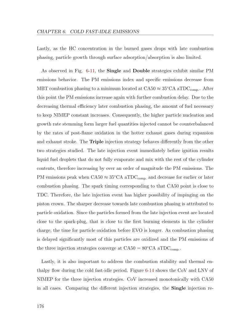
CHAPTER 6. COLD FAST-IDLE EMISSIONS
Lastly, as the HC concentration in the burned gases drops with late combustion
phasing, particle growth through surface adsorption/absorption is also limited.
As observed in Fig. 6-11, the Single and Double strategies exhibit similar PM
emissions behavior. The PM emissions index and specific emissions decrease from
MBT combustion phasing to a minimum located at CA50 ≈ 35◦CA aTDCcomp.. After
this point the PM emissions increase again with further combustion delay. Due to the
decreasing thermal efficiency later combustion phasing, the amount of fuel necessary
to keep NIMEP constant increases. Consequently, the higher particle nucleation and
growth rate stemming form larger fuel quantities injected cannot be counterbalanced
by the rates of post-flame oxidation in the hotter exhaust gases during expansion
and exhaust stroke. The Triple injection strategy behaves differently from the other
two strategies studied. The late injection event immediately before ignition results
liquid fuel droplets that do not fully evaporate and mix with the rest of the cylinder
contents, therefore increasing by over an order of magnitude the PM emissions. The
PM emissions peak when CA50 ≈ 35◦CA aTDCcomp. and decrease for earlier or later
combustion phasing. The spark timing corresponding to that CA50 point is close to
TDC. Therefore, the late injection event has higher possibility of impinging on the
piston crown. The sharper decrease towards late combustion phasing is attributed to
particle oxidation. Since the particles formed from the late injection event are located
close to the spark-plug, that is close to the first burning elements in the cylinder
charge, the time for particle oxidation before EVO is longer. As combustion phasing
is delayed significantly most of this particles are oxidized and the PM emissions of
the three injection strategies converge at CA50 = 80◦CA aTDCcomp..
Lastly, it is also important to address the combustion stability and thermal en-
thalpy flow during the cold fast-idle period. Figure 6-14 shows the CoV and LNV of
NIMEP for the three injection strategies. CoV increased monotonically with CA50
in all cases. Comparing the different injection strategies, the Single injection re-
176
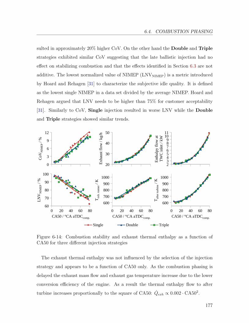
6.4. COMBUSTION PHASING
sulted in approximately 20% higher CoV. On the other hand the Double and Triple
strategies exhibited similar CoV suggesting that the late ballistic injection had no
effect on stabilizing combustion and that the effects identified in Section 6.3 are not
additive. The lowest normalized value of NIMEP (LNVNIMEP) is a metric introduced
by Hoard and Rehagen [31] to characterize the subjective idle quality. It is defined
as the lowest single NIMEP in a data set divided by the average NIMEP. Hoard and
Rehagen argued that LNV needs to be higher than 75% for customer acceptability
[31]. Similarly to CoV, Single injection resulted in worse LNV while the Double
and Triple strategies showed similar trends.
Single Double Triple
Exh
aust
flo
w /
kg/h
20
30
40
50
Tex
h. r
unne
r / K
600
700
800
900
1000
CA50 / °CA aTDCcomp.
0 20 40 60 80
Taf
ter
turb
ine /
K
600
700
800
900
1000
CA50 / °CA aTDCcomp.
0 20 40 60 80
Ent
hal
py fl
ow a
t T
WC
inle
t / k
W23456789
1011
CoV
NIM
EP /
%
0
3
6
9
12
LNV
NIM
EP /
%
60
70
80
90
100
CA50 / °CA aTDCcomp.
0 20 40 60 80
Figure 6-14: Combustion stability and exhaust thermal enthalpy as a function ofCA50 for three different injection strategies
The exhaust thermal enthalpy was not influenced by the selection of the injection
strategy and appears to be a function of CA50 only. As the combustion phasing is
delayed the exhaust mass flow and exhaust gas temperature increase due to the lower
conversion efficiency of the engine. As a result the thermal enthalpy flow to after
turbine increases proportionally to the square of CA50: Qexh ∝ 0.002 · CA502.
177
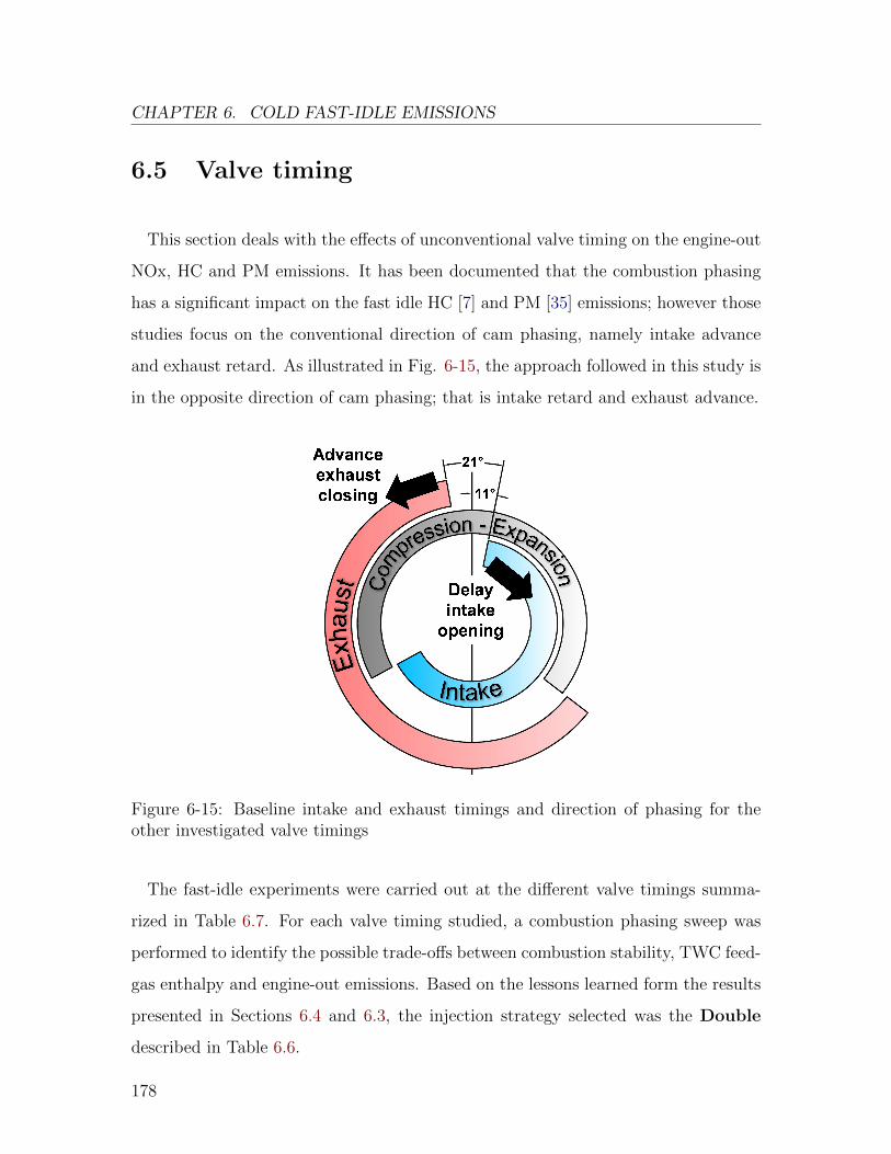
CHAPTER 6. COLD FAST-IDLE EMISSIONS
6.5 Valve timing
This section deals with the effects of unconventional valve timing on the engine-out
NOx, HC and PM emissions. It has been documented that the combustion phasing
has a significant impact on the fast idle HC [7] and PM [35] emissions; however those
studies focus on the conventional direction of cam phasing, namely intake advance
and exhaust retard. As illustrated in Fig. 6-15, the approach followed in this study is
in the opposite direction of cam phasing; that is intake retard and exhaust advance.
Figure 6-15: Baseline intake and exhaust timings and direction of phasing for theother investigated valve timings
The fast-idle experiments were carried out at the different valve timings summa-
rized in Table 6.7. For each valve timing studied, a combustion phasing sweep was
performed to identify the possible trade-offs between combustion stability, TWC feed-
gas enthalpy and engine-out emissions. Based on the lessons learned form the results
presented in Sections 6.4 and 6.3, the injection strategy selected was the Double
described in Table 6.6.
178
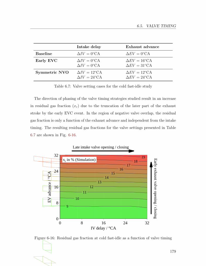
6.5. VALVE TIMING
Intake delay Exhaust advance
Baseline ∆IV = 0◦CA ∆EV = 0◦CA
Early EVC ∆IV = 0◦CA ∆EV = 16◦CA∆IV = 0◦CA ∆EV = 31◦CA
Symmetric NVO ∆IV = 12◦CA ∆EV = 12◦CA∆IV = 24◦CA ∆EV = 24◦CA
Table 6.7: Valve setting cases for the cold fast-idle study
The direction of phasing of the valve timing strategies studied result in an increase
in residual gas fraction (xr) due to the truncation of the later part of the exhaust
stroke by the early EVC event. In the region of negative valve overlap, the residual
gas fraction is only a function of the exhaust advance and independent from the intake
timing. The resulting residual gas fractions for the valve settings presented in Table
6.7 are shown in Fig. 6-16.
19
17
15
13
9
10
18
16
14
12
11
EV
ad
vanc
e /
°CA
32
24
16
8
0
IV delay / °CA0 8 16 24 32
Late intake valve opening / closing
Early exha
ust valve ope
ning / closing
xr in % (Simulation)
Figure 6-16: Residual gas fraction at cold fast-idle as a function of valve timing
179
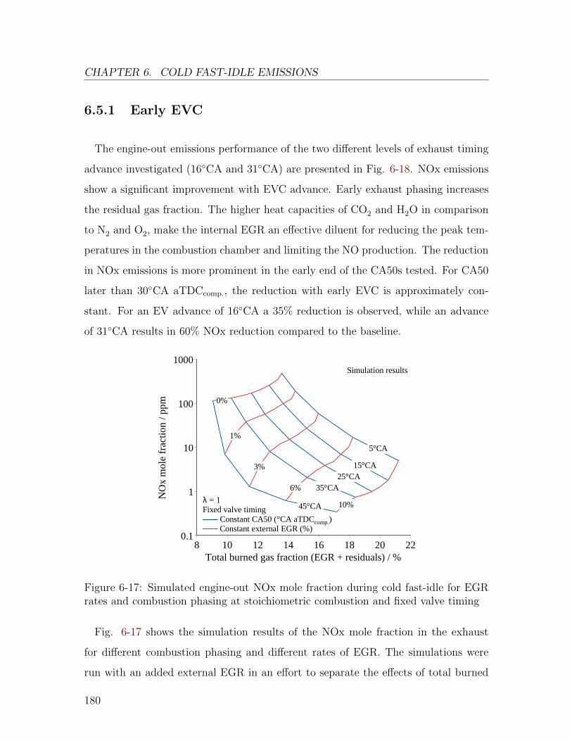
CHAPTER 6. COLD FAST-IDLE EMISSIONS
6.5.1 Early EVC
The engine-out emissions performance of the two different levels of exhaust timing
advance investigated (16◦CA and 31◦CA) are presented in Fig. 6-18. NOx emissions
show a significant improvement with EVC advance. Early exhaust phasing increases
the residual gas fraction. The higher heat capacities of CO2 and H2O in comparison
to N2 and O2, make the internal EGR an effective diluent for reducing the peak tem-
peratures in the combustion chamber and limiting the NO production. The reduction
in NOx emissions is more prominent in the early end of the CA50s tested. For CA50
later than 30◦CA aTDCcomp., the reduction with early EVC is approximately con-
stant. For an EV advance of 16◦CA a 35% reduction is observed, while an advance
of 31◦CA results in 60% NOx reduction compared to the baseline.
NO
x m
ole
frac
tion
/ p
pm
0.1
1
10
100
1000
Total burned gas fraction (EGR + residuals) / %8 10 12 14 16 18 20 22
λ = 1Fixed valve timing
Constant CA50 (°CA aTDCcomp.) Constant external EGR (%)
45°CA
15°CA25°CA
35°CA
5°CA
0%
1%
3%
6%
10%
Simulation results
Figure 6-17: Simulated engine-out NOx mole fraction during cold fast-idle for EGRrates and combustion phasing at stoichiometric combustion and fixed valve timing
Fig. 6-17 shows the simulation results of the NOx mole fraction in the exhaust
for different combustion phasing and different rates of EGR. The simulations were
run with an added external EGR in an effort to separate the effects of total burned
180
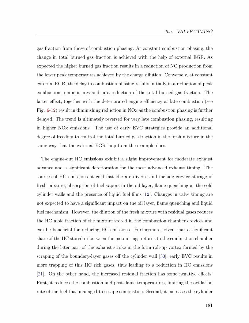
6.5. VALVE TIMING
gas fraction from those of combustion phasing. At constant combustion phasing, the
change in total burned gas fraction is achieved with the help of external EGR. As
expected the higher burned gas fraction results in a reduction of NO production from
the lower peak temperatures achieved by the charge dilution. Conversely, at constant
external EGR, the delay in combustion phasing results initially in a reduction of peak
combustion temperatures and in a reduction of the total burned gas fraction. The
latter effect, together with the deteriorated engine efficiency at late combustion (see
Fig. 6-12) result in diminishing reduction in NOx as the combustion phasing is further
delayed. The trend is ultimately reversed for very late combustion phasing, resulting
in higher NOx emissions. The use of early EVC strategies provide an additional
degree of freedom to control the total burned gas fraction in the fresh mixture in the
same way that the external EGR loop from the example does.
The engine-out HC emissions exhibit a slight improvement for moderate exhaust
advance and a significant deterioration for the most advanced exhaust timing. The
sources of HC emissions at cold fast-idle are diverse and include crevice storage of
fresh mixture, absorption of fuel vapors in the oil layer, flame quenching at the cold
cylinder walls and the presence of liquid fuel films [12]. Changes in valve timing are
not expected to have a significant impact on the oil layer, flame quenching and liquid
fuel mechanism. However, the dilution of the fresh mixture with residual gases reduces
the HC mole fraction of the mixture stored in the combustion chamber crevices and
can be beneficial for reducing HC emissions. Furthermore, given that a significant
share of the HC stored in-between the piston rings returns to the combustion chamber
during the later part of the exhaust stroke in the form roll-up vortex formed by the
scraping of the boundary-layer gases off the cylinder wall [30], early EVC results in
more trapping of this HC rich gases, thus leading to a reduction in HC emissions
[21]. On the other hand, the increased residual fraction has some negative effects.
First, it reduces the combustion and post-flame temperatures, limiting the oxidation
rate of the fuel that managed to escape combustion. Second, it increases the cylinder
181
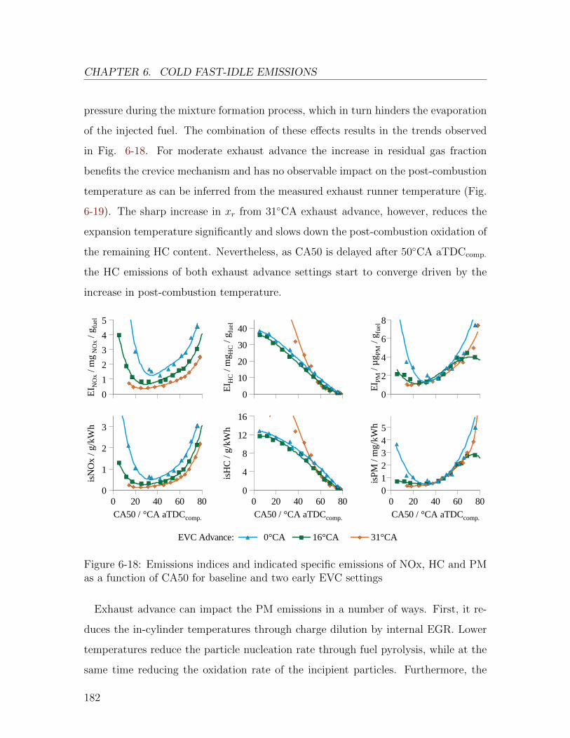
CHAPTER 6. COLD FAST-IDLE EMISSIONS
pressure during the mixture formation process, which in turn hinders the evaporation
of the injected fuel. The combination of these effects results in the trends observed
in Fig. 6-18. For moderate exhaust advance the increase in residual gas fraction
benefits the crevice mechanism and has no observable impact on the post-combustion
temperature as can be inferred from the measured exhaust runner temperature (Fig.
6-19). The sharp increase in xr from 31◦CA exhaust advance, however, reduces the
expansion temperature significantly and slows down the post-combustion oxidation of
the remaining HC content. Nevertheless, as CA50 is delayed after 50◦CA aTDCcomp.
the HC emissions of both exhaust advance settings start to converge driven by the
increase in post-combustion temperature.
EVC Advance: 0°CA 16°CA 31°CA
EI H
C /
mg H
C /
g fue
l
0
10
20
30
40
isH
C /
g/kW
h
0
4
8
12
16
CA50 / °CA aTDCcomp.
0 20 40 60 80
isP
M /
mg
/kW
h
012345
CA50 / °CA aTDCcomp.
0 20 40 60 80
EI P
M /
µg P
M /
g fue
l
0
2
4
6
8
EI N
Ox
/ mg
NO
x / g
fuel
0
1
2
3
4
5
isN
Ox
/ g/k
Wh
0
1
2
3
CA50 / °CA aTDCcomp.
0 20 40 60 80
Figure 6-18: Emissions indices and indicated specific emissions of NOx, HC and PMas a function of CA50 for baseline and two early EVC settings
Exhaust advance can impact the PM emissions in a number of ways. First, it re-
duces the in-cylinder temperatures through charge dilution by internal EGR. Lower
temperatures reduce the particle nucleation rate through fuel pyrolysis, while at the
same time reducing the oxidation rate of the incipient particles. Furthermore, the
182
6.5. VALVE TIMING
effect exhaust advance on the post-flame oxidation of the HC content can affect the
particle growth by surface agglomeration of HC on the formed particles. These com-
peting effects result in the PM trends observed in Fig. 6-18. Particulate emissions
show a significant improvement with exhaust advance for CA50 timings earlier than
20◦CA aTDCcomp.. From CA50 in the range of 20− 70◦CA aTDCcomp., the PM emis-
sions are independent of the valve timing. The latest CA50 point tested suggests an
impact of early EVC on particle reduction; however, given the combustion instability
at this late spark timing the significance of that point is reduced.
EVC Advance: 0°CA 16°CA 31°CA
Exh
aust
flo
w /
kg/h
20
30
40
50
Tex
h. r
unne
r / K
600
700
800
900
1000
CA50 / °CA aTDCcomp.
0 20 40 60 80
Taf
ter
turb
ine /
K
600
700
800
900
1000
CA50 / °CA aTDCcomp.
0 20 40 60 80
Ent
hal
py fl
ow a
t T
WC
inle
t / k
W
02468
101214
CoV
NIM
EP /
%
0
3
6
9
12
15
LNV
NIM
EP /
%
50
60
70
80
90
100
CA50 / °CA aTDCcomp.
0 20 40 60 80
Figure 6-19: Combustion stability and exhaust thermal enthalpy as a function ofCA50 for baseline and two early EVC settings
Figure 6-19 shows the combustion stability metrics and the feed gas enthalpy flow
to the catalyst. The increase in residual gas fraction from early EVC reduces the
flame propagation speed and consequently deteriorates the CoV and LNV of NIMEP.
The moderate exhaust advance increases the slope of the CoV trace in 20%, while the
most advanced EV results in a similar increase in slope with an additional offset of
3.5% CoV. Regarding the enthalpy flow, moderate exhaust advance has no influence
183
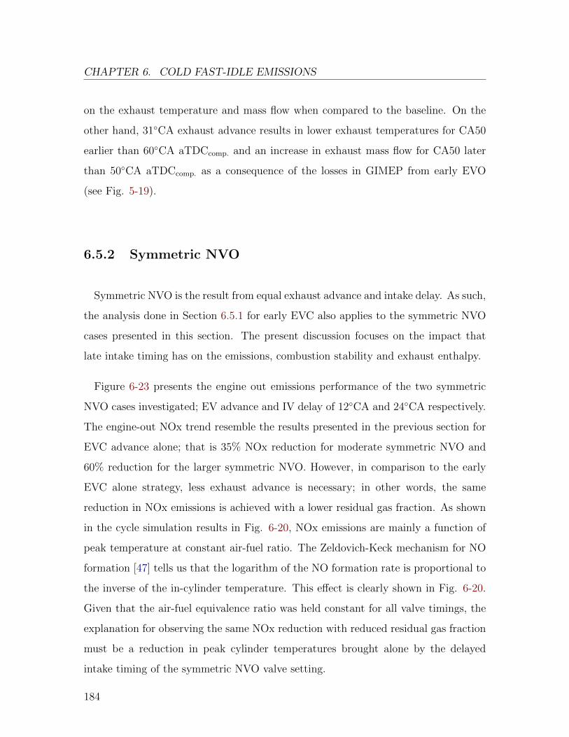
CHAPTER 6. COLD FAST-IDLE EMISSIONS
on the exhaust temperature and mass flow when compared to the baseline. On the
other hand, 31◦CA exhaust advance results in lower exhaust temperatures for CA50
earlier than 60◦CA aTDCcomp. and an increase in exhaust mass flow for CA50 later
than 50◦CA aTDCcomp. as a consequence of the losses in GIMEP from early EVO
(see Fig. 5-19).
6.5.2 Symmetric NVO
Symmetric NVO is the result from equal exhaust advance and intake delay. As such,
the analysis done in Section 6.5.1 for early EVC also applies to the symmetric NVO
cases presented in this section. The present discussion focuses on the impact that
late intake timing has on the emissions, combustion stability and exhaust enthalpy.
Figure 6-23 presents the engine out emissions performance of the two symmetric
NVO cases investigated; EV advance and IV delay of 12◦CA and 24◦CA respectively.
The engine-out NOx trend resemble the results presented in the previous section for
EVC advance alone; that is 35% NOx reduction for moderate symmetric NVO and
60% reduction for the larger symmetric NVO. However, in comparison to the early
EVC alone strategy, less exhaust advance is necessary; in other words, the same
reduction in NOx emissions is achieved with a lower residual gas fraction. As shown
in the cycle simulation results in Fig. 6-20, NOx emissions are mainly a function of
peak temperature at constant air-fuel ratio. The Zeldovich-Keck mechanism for NO
formation [47] tells us that the logarithm of the NO formation rate is proportional to
the inverse of the in-cylinder temperature. This effect is clearly shown in Fig. 6-20.
Given that the air-fuel equivalence ratio was held constant for all valve timings, the
explanation for observing the same NOx reduction with reduced residual gas fraction
must be a reduction in peak cylinder temperatures brought alone by the delayed
intake timing of the symmetric NVO valve setting.
184
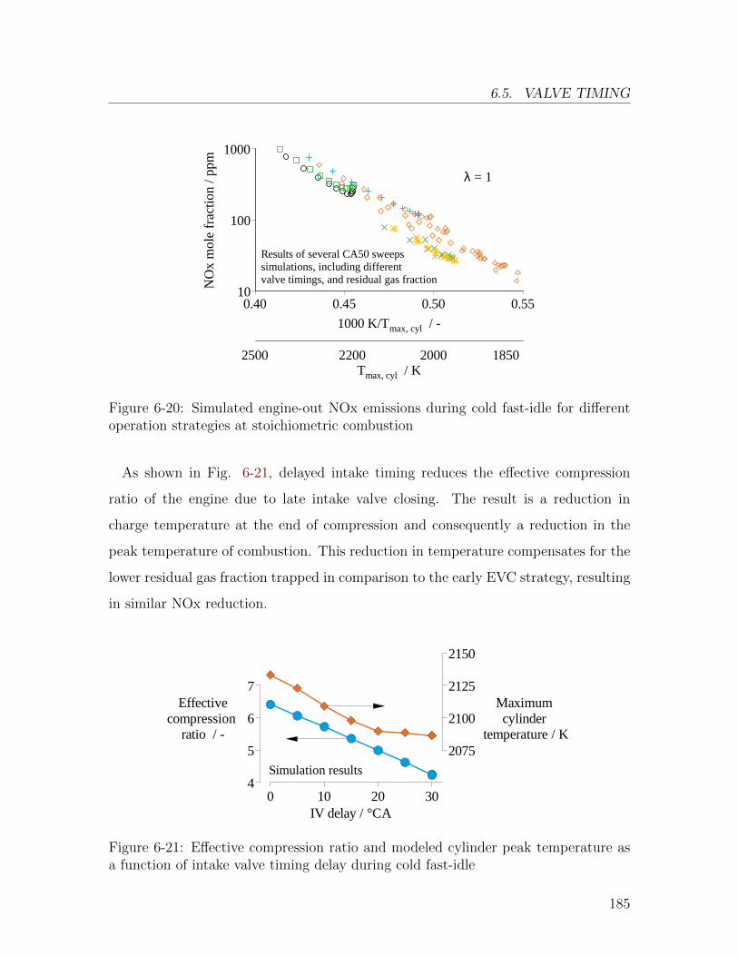
6.5. VALVE TIMING
Results of several CA50 sweepssimulations, including different valve timings, and residual gas fractionN
Ox
mol
e fr
actio
n / p
pm
10
100
1000
1000 K/Tmax, cyl / -
0.40 0.45 0.50 0.55
λ = 1
Tmax, cyl / K2200 18502500 2000
Figure 6-20: Simulated engine-out NOx emissions during cold fast-idle for differentoperation strategies at stoichiometric combustion
As shown in Fig. 6-21, delayed intake timing reduces the effective compression
ratio of the engine due to late intake valve closing. The result is a reduction in
charge temperature at the end of compression and consequently a reduction in the
peak temperature of combustion. This reduction in temperature compensates for the
lower residual gas fraction trapped in comparison to the early EVC strategy, resulting
in similar NOx reduction.
Simulation results
IV delay / °CA0 10 20 30
Effectivecompression
ratio / -
4
5
6
7Maximum cylinder
temperature / K2075
2100
2125
2150
Figure 6-21: Effective compression ratio and modeled cylinder peak temperature asa function of intake valve timing delay during cold fast-idle
185
CHAPTER 6. COLD FAST-IDLE EMISSIONS
Regarding the HC emissions (Fig. 6-23, middle), the moderate symmetric NVO
valve setting results in a reduction of HC emissions for combustion phasing with a
CA50 later than 20◦CA aTDCcomp.. For the larger NVO setting, the HC emissions
deteriorate significantly as it was the case for the early EVC strategy. To understand
the differences between the HC emissions behavior of the baseline, early EVC and
symmetric NVO, it is worth to take a closer look at the traces of the HC mole fraction.
Fig 6-22 shows the crank-angle resolved HC mole fraction and mass emissions during
the exhaust stroke for the three valve timing settings. The HC concentration traces
feature two peaks; the first one related to the HC bulk concentration in the burned
gases; the second one associated to the roll-up vortex caused by the scraping of
the HC-rich boundary-layer formed by the remaining of the crevice HC and those
desorbing and evaporating from the cylinder wall [30].
In comparison to the baseline, early EVC results in marginally lower HC emissions,
while the symmetric NVO strategy shows a greater improvement in HC emissions
than early EVC alone. The cumulative HC mass trace of the case with delayed intake
timing (symmetric NVO) exhibits a lower blow-down value, compared to the stock
intake timing (baseline and early EVC). The blow-down trend can be explained as
follows: Late intake timing reduces the in-cylinder pressure at EVO (due to the lower
effective compression ratio), therefore lowering the exhausted mass during blow-down.
On the other hand, early exhaust timing lowers the HC concentration through charge
dilution with residual gases, while at the same time increasing the exhausted mass
during blow-down due to higher cylinder pressures at the advanced EVO. Moreover,
advanced exhaust timing results in flow reversal close to the maximum exhaust valve
lift. As a result, the exhausted mass is higher towards the end of the exhaust event,
and slope of the cumulative HC trace is steeper for the advanced exhaust timing.
Nevertheless, the end-of-stroke HC peak concentrations are lower for the symmetric
NVO in comparison to early EVC.
186
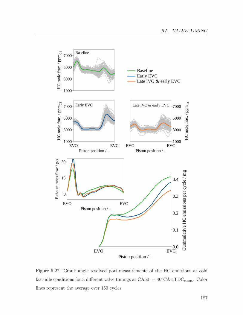
6.5. VALVE TIMING
HC
mol
e fr
ac. /
ppm
C1
1000
3000
5000
7000
Piston position / -EVO EVC
Late IVO & early EVC
HC
mol
e fr
ac. /
ppm
C1
1000
3000
5000
7000
Piston position / -EVO EVC
Early EVC
HC
mol
e fr
ac. /
ppm
C1
1000
3000
5000
7000Baseline
Cum
mul
ativ
e H
C e
mis
sion
s pe
r cy
cle
/ mg
0.0
0.1
0.2
0.3
0.4
Piston position / -EVO EVC
Baseline Early EVC Late IVO & early EVC
Exh
aust
mas
s fl
ow /
g/s
0
15
30
Piston position / -EVO EVC
Figure 6-22: Crank angle resolved port-measurements of the HC emissions at cold
fast-idle conditions for 3 different valve timings at CA50 = 40◦CA aTDCcomp.. Color
lines represent the average over 150 cycles
187
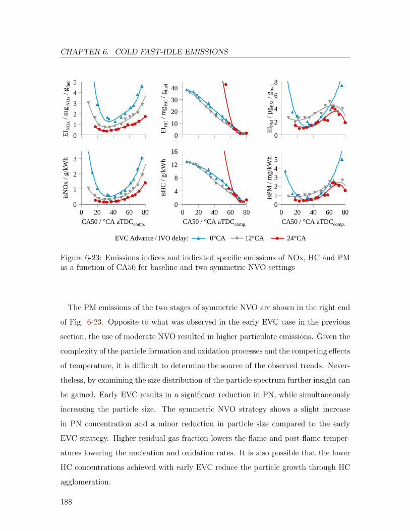
CHAPTER 6. COLD FAST-IDLE EMISSIONS
EVC Advance / IVO delay: 0°CA 12°CA 24°CA
EI H
C /
mg H
C /
g fue
l
0
10
20
30
40
isH
C /
g/kW
h
0
4
8
12
16
CA50 / °CA aTDCcomp.
0 20 40 60 80
isP
M /
mg
/kW
h
012345
CA50 / °CA aTDCcomp.
0 20 40 60 80
EI P
M /
µg P
M /
g fue
l
0
2
4
6
8
EI N
Ox
/ mg
NO
x / g
fuel
0
1
2
3
4
5
isN
Ox
/ g/k
Wh
0
1
2
3
CA50 / °CA aTDCcomp.
0 20 40 60 80
Figure 6-23: Emissions indices and indicated specific emissions of NOx, HC and PMas a function of CA50 for baseline and two symmetric NVO settings
The PM emissions of the two stages of symmetric NVO are shown in the right end
of Fig. 6-23. Opposite to what was observed in the early EVC case in the previous
section, the use of moderate NVO resulted in higher particulate emissions. Given the
complexity of the particle formation and oxidation processes and the competing effects
of temperature, it is difficult to determine the source of the observed trends. Never-
theless, by examining the size distribution of the particle spectrum further insight can
be gained. Early EVC results in a significant reduction in PN, while simultaneously
increasing the particle size. The symmetric NVO strategy shows a slight increase
in PN concentration and a minor reduction in particle size compared to the early
EVC strategy. Higher residual gas fraction lowers the flame and post-flame temper-
atures lowering the nucleation and oxidation rates. It is also possible that the lower
HC concentrations achieved with early EVC reduce the particle growth through HC
agglomeration.
188
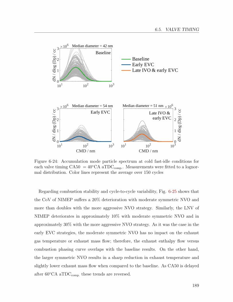
6.5. VALVE TIMING
CMD / nm101 102 103
dN /
dlog
(D
p) /
cc
106
0
1
2
3
CMD / nm101 102 103
dN /
dlog
(D
p) /
cc
106
0
1
2
3
CMD / nm101 102 103
dN /
dlog
(D
p) /
cc
106
0
1
2
3
Baseline
Early EVC Late IVO & early EVC
Median diameter = 54 nm Median diameter = 51 nm
Median diameter = 42 nm
Baseline Early EVC Late IVO & early EVC
Figure 6-24: Accumulation mode particle spectrum at cold fast-idle conditions foreach valve timing CA50 = 40◦CA aTDCcomp.. Measurements were fitted to a lognor-mal distribution. Color lines represent the average over 150 cycles
Regarding combustion stability and cycle-to-cycle variability, Fig. 6-25 shows that
the CoV of NIMEP suffers a 20% deterioration with moderate symmetric NVO and
more than doubles with the more aggressive NVO strategy. Similarly, the LNV of
NIMEP deteriorates in approximately 10% with moderate symmetric NVO and in
approximately 30% with the more aggressive NVO strategy. As it was the case in the
early EVC strategies, the moderate symmetric NVO has no impact on the exhaust
gas temperature or exhaust mass flow; therefore, the exhaust enthalpy flow versus
combustion phasing curve overlaps with the baseline results. On the other hand,
the larger symmetric NVO results in a sharp reduction in exhaust temperature and
slightly lower exhaust mass flow when compared to the baseline. As CA50 is delayed
after 60◦CA aTDCcomp. these trends are reversed.
189
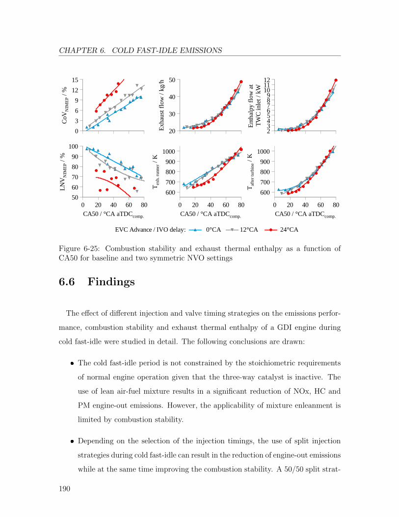
CHAPTER 6. COLD FAST-IDLE EMISSIONS
EVC Advance / IVO delay: 0°CA 12°CA 24°CA
Exh
aust
flo
w /
kg/h
20
30
40
50
Tex
h. r
unne
r / K
600
700
800
900
1000
CA50 / °CA aTDCcomp.
0 20 40 60 80
Taf
ter
turb
ine /
K
600
700
800
900
1000
CA50 / °CA aTDCcomp.
0 20 40 60 80
Ent
hal
py fl
ow a
t T
WC
inle
t / k
W
23456789
101112
CoV
NIM
EP /
%
0
3
6
9
12
15
LNV
NIM
EP /
%
50
60
70
80
90
100
CA50 / °CA aTDCcomp.
0 20 40 60 80
Figure 6-25: Combustion stability and exhaust thermal enthalpy as a function ofCA50 for baseline and two symmetric NVO settings
6.6 Findings
The effect of different injection and valve timing strategies on the emissions perfor-
mance, combustion stability and exhaust thermal enthalpy of a GDI engine during
cold fast-idle were studied in detail. The following conclusions are drawn:
� The cold fast-idle period is not constrained by the stoichiometric requirements
of normal engine operation given that the three-way catalyst is inactive. The
use of lean air-fuel mixture results in a significant reduction of NOx, HC and
PM engine-out emissions. However, the applicability of mixture enleanment is
limited by combustion stability.
� Depending on the selection of the injection timings, the use of split injection
strategies during cold fast-idle can result in the reduction of engine-out emissions
while at the same time improving the combustion stability. A 50/50 split strat-
190
6.6. FINDINGS
egy, where the first injection event occurs during maximum intake valve lift and
the second close to bottom dead center exhibited the best performance. Earlier
injection timings may result in interaction between the piston crown and the
fuel stray leading to a drastic increase in particulate formation and emissions.
The use of a very short injection immediately before spark timing improves the
combustion stability but deteriorates significantly the PM emissions.
� The engine-out emissions have a high sensitivity to combustion phasing. Ini-
tial retard results in a significant reduction in NOx emissions up CA50 ≈
40◦CA aTDCcomp.. After this point the increase in fuel use from the lower
engine efficiency and the reduction of residual gas mass fraction from the hotter
exhaust gases reverse the trend leading to an increase in NOx emissions as the
combustion phasing is further retarded. HC emissions on the other hand exhibit
a monotonic decrease with combustion phasing; as the expansion and exhaust
temperatures increase with late spark timing, the post-oxidation rate of HC
increases. PM emissions exhibit a similar dependence on CA50 as NOx. PM
emissions drop sharply as combustion is initially delayed achieving a minimum
between 20 and 40◦CA aTDCcomp.; thereafter, the larger amount of fuel neces-
sary to compensate the decrease in engine efficiency promote the formation of
fuel films and increase the PM emissions.
� The thermal enthalpy flow of the feed-gas to TWC increases proportionally to
the square of CA50.
� Moderate exhaust valve timing advance is beneficial for engine-out emissions,
has no impact on the exhaust enthalpy and deteriorates slightly combustion sta-
bility. The observed trends are mainly a result of the higher residual gas fraction
of early EVC strategies. More aggressive exhaust timing advance reduces the
expansion and exhaust temperatures significantly resulting in an increase in HC
emissions.
191
CHAPTER 6. COLD FAST-IDLE EMISSIONS
� The combined use of intake timing delay and exhaust valve advance, dubbed
symmetric NVO, exhibits the same emissions trends as early EVC alone. The
decreased effective compression ratio from late IVO reduces slightly the peak
cylinder temperature and pressure. As a result, similar improvements in NOx
and HC can be achieved at lower residual gas fraction, when compared to the
early EVC valve settings.
� There are clear tradeoffs present between engine-out emission, combustion sta-
bility and exhaust enthalpy flow. To minimize NOx emissions high residual gas
fractions are beneficial; however HC emissions and combustion stability can be
significantly affected. The reduction of HC emissions and of exhaust enthalpy
is favored at very late combustion phasing; however, the emissions of PM and
NOx increase and the combustion stability is deteriorated. PM emissions are
favored at relatively early combustion phasing CA50 ≈ 30◦CA aTDCcomp.; on
the other hand this level of exhaust enthalpy flow would result in a longer light-
off time of the catalytic converter, increasing the cumulative emissions of NOx
and HC.
192
Chapter 7
Conclusion
The cold-start phase is responsible for a disproportionate share of the pollutant
emissions of internal combustion engines. The purpose of the work presented in
this dissertation was to expand the understanding of the mechanisms leading to the
production and emission of regulated pollutants (CO, NOx, HC, and PM) during the
cold-start phase of light-duty gasoline direct injection engines and to investigate the
potential of different operation strategies for their mitigation.
The results indicate that the pollutant formation mechanisms have a strong depen-
dence on the mixture formation process and on the temperature and pressure history
during combustion. The strategies with the largest potential for the reduction of pol-
lutant emissions during cold-start are the use of unconventional valve timing featuring
a large, symmetric, negative valve overlap and of delayed combustion phasing.
The following sections provide an overview of the experimental approach used for
the investigations, present the key contributions of this study and their significance,
and propose recommendations for future research in the area of cold-start emissions
of gasoline direct injection engines.
193
CHAPTER 7. CONCLUSION
7.1 Overview
The experimental research was divided into the two phases of the cold-start period,
the engine crank-start and the steady-state fast-idle. The experimental engine results
were supplemented by modeling of the processes that were not measurable during the
experiments, such as the crank-angle resolved exhaust mass flow rate, the cylinder
temperature and the residual gas fraction. The experiments performed can be grouped
into three categories.
1. Cycle-by-cycle experiments: The first three combustion cycles during the
crank-start process were studied under several operation parameters including
the amount of fuel injected, injection timing, combustion phasing, fuel pressure,
throttle position and engine speed. The cycle-resolved mass emissions of CO,
NOx, HC and PM were recorded during the experiments as a function of the
aforementioned parameters.
2. Crank-start experiments: Complete crank-start experiments were conducted
for four different valve settings including the stock valve setting of the engine as
a baseline, delayed intake timing, advanced exhaust timing and a combination
of late intake with early exhaust timings, dubbed negative valve overlap (NVO).
The combustion phasing and the combustion equivalence ratio were kept con-
stant across the different valve settings. The cumulative engine-out pollutant
emissions were recorded.
3. Fast-idle experiments: The steady-state experiments at 20◦C, 2.3 bar of
NIMEP and an engine speed of 1200 rpm were carried out for different en-
gine operating parameters including equivalence ratio, split injection schedules,
combustion phasing and valve timing. The output variables of interest were the
pollutant emissions flow rates as well at the enthalpy flow of the exhaust gas at
the inlet of the three-way catalyst.
194
7.2. CONTRIBUTIONS
7.2 Contributions
This section presents the main contributions of this study in explaining the mech-
anisms for pollutant formation during cold-start and identifying the emissions reduc-
tion potential of different operation strategies in gasoline direct injection engines. The
findings are presented separately for the cold crank-start and the fast-idle phases.
7.2.1 Cold crank-start in GDI engines
Compared to all other engine operation regimes, the cold crank-start experiences
two extreme conditions: the lowest temperature and lowest engine speed. The evap-
oration process of the fuel spray is strongly dependent on the combustion chamber
surfaces and bulk gas temperatures as well as on the charge turbulence. Consequently,
the mixture formation process is negatively impacted during cold crank-start and sig-
nificant over-fueling is necessary to obtain an ignitable mixture.
The fuel mass required to obtain robust combustion in the 1st cycle during cold
crank-start depends on the injection schedule, as it affects the degree of charge strat-
ification. In the case of fuel injection during the intake or early compression strokes,
approximately 75 mg of fuel are required; this amounts to circa 2.5 times the amount
of fuel necessary to form a stoichiometric air-fuel mixture, that is, if all the fuel would
evaporate and fully mix. The fraction of the fuel injected that evaporates and par-
ticipates in the combustion process is approximately one third of the total injected
amount. Of that third of fuel injected being converted to CO2 and other combustion
products, only a quarter, or around 8% of the total injected fuel energy, is converted
to work. The remaining part of the energy released from the fuel is lost as heat
transfer to the cold cylinder walls or is exhausted in the form of sensible enthalpy.
In the case of mixture stratification through late injection, the reduction of spray
195
CHAPTER 7. CONCLUSION
interaction with the liner increases the fuel mass participating in combustion.
The use of higher fuel pressure reduces the fuel spray droplet size and increases
the turbulence during the injection event. Higher engine speeds result in higher
turbulence during the intake and compression processes. Both effects improve the
evaporation process, increasing the fraction of fuel being oxidized to CO2.
The 1st cycle emissions of NOx, HC and PM, exhibit a high sensitivity to the in-
jection and spark timings. The injection timing determines the location and degree
of the interaction between the fuel spray and the combustion chamber surfaces. In-
jection events during the early part of the intake stroke result in spray interaction
with the piston crown which deteriorates the fuel evaporation and, in some cases,
leads to misfiring of the cycle. As the injection timing is delayed to the mid part of
the intake stroke, the interaction of the spray with the intake valve becomes domi-
nant, resulting in a sharp increase in HC emissions. However, the spray/intake valve
interaction does not affect the PM emissions and results in a reduction of the peak
temperatures, leading to lower NO production. Injection events near bottom dead
center result in the best emissions performance. Further delay in the injection timing
results in increasing mixture stratification leading to an increased share of unburned
HC and a higher formation rate of particulates. NO formation, on the other hand, is
reduced as the mixture becomes more stratified.
Spark timing has a direct influence on the temperature history of the combustion
process and on the time available for the post-combustion processes to occur before
opening of the exhaust valve. Delaying the combustion phasing reduces the time
available for particle formation through fuel pyrolysis and affects the formation and
oxidation rates through changes in temperature. The end result is a significant re-
duction of PM emissions with late combustion phasing. Late spark timing reduces
the peak cylinder temperatures leading to a reduction in NO formation. On the other
hand, HC emissions are insensitive to spark timing for most of the range studied.
196
7.2. CONTRIBUTIONS
For the 2nd and 3rd cycles, the warming of the combustion chamber surfaces and
the presence of residual fuel from previous injection events results in a reduction
in the over-fueling requirement for robust combustion. The over-fueling required
corresponds to 1.7 and 1.5 times the stoichiometric fuel amount, for the 2nd and
3rd cycles respectively. The amount of residual fuel leftover from the 1st cycle that is
available to participate in the 2nd cycle mixture formation accounts for approximately
20% of the fuel participating in combustion during the 2nd cycle. Additionally, the
warming up of the cylinder liner during the 1st cycle combustion and exhaust processes
has a large influence on the evaporation process of the 2nd cycle fuel injection; an
increase in roughly 100 J of heat transfer to the walls during the 1st cycle results in
an additional 1 mg of fuel evaporating from the injection event in the 2nd cycle.
The emissions trends for the 2nd and 3rd cycles as a function of the injection timing
and combustion phasing are very similar to those of the 1st cycle described above.
However, the magnitude of the emissions changes significantly as the crank-start goes
from the 1st to the 3rd cycle. NOx emissions are reduced as the engine runs up to
the speed flare due to a reduction in the work output from the lower intake manifold
pressure. The peaks observed in the HC emissions as a function of the start of
injection are reduced in magnitude as the engine accelerates; however, the minimum
value stays at a comparable level for all three cycles. Lastly, PM emissions are reduced
by more than an order of magnitude as the engine accelerates during crank-start.
The use of unconventional valve timing provides an additional degree of freedom
for controlling the engine-out emissions during cold crank-start. Delaying the intake
valve opening decreases the cylinder pressure in the early part of the intake stroke
favoring the flash boiling of volatile fuel species. It also increases the air speed through
the intake valve increasing the turbulent intensity , and results in higher temperatures
at the end of the intake stroke. Additionally, intake cam retarding delays the closing
of the intake valve. As a result, the volumetric efficiency is reduced and less fuel
197
CHAPTER 7. CONCLUSION
mass is required for robust combustion. These mechanisms lead to an improved
mixture formation process, reducing the formation of fuel films, and therefore of HC
and PM emissions. The reduced effective compression ratio also leads to lower peak
temperatures during combustion which slow down the formation of NO.
Advancing the exhaust cam phasing increases the amount of burned gases trapped
at the end of the exhaust stroke due to the earlier exhaust valve closing. The early
exhaust timing strategy has no impact on the mixture formation of the 1st cycle, due
to the absence of residuals. From the 2nd cycle on, advance exhaust timing improves
the NOx emissions due to the lower temperatures achieved by the dilution of the
fresh mixture with the larger amount of burned gases. On the other hand, early
exhaust valve closing resulted in worse HC and PM emissions during crank-start.
The combined strategy of late intake phasing with early exhaust phasing results in a
significant reduction in NOx emissions and in an improvement of HC and PM similar
to what was observed by only delaying the intake cam phasing.
7.2.2 Cold fast-idle in GDI engines
The cold fast-idle is a critical period in the engine homologation procedure. The
main objective during the 20-second fast-idling period before the first acceleration
event in the driving schedule is to provide enough thermal enthalpy to the three-way
catalyst to achieve a fast light-off. Simultaneously, due to the catalytic inactivity
of the after-treatment system, the engine-out emissions must be minimized and the
engine stability must be preserved.
Due to the three-way catalyst inactivity, the cold fast-idle is not constrained to
stoichiometric operation. The use of a slightly fuel-lean equivalence ratio (λ = 1.05)
provides an oxidizing environment adequate for the reduction of HC and PM emis-
sions, while it has little impact on the NO formation. The use of an even split injection
198
7.2. CONTRIBUTIONS
strategy, with both injection events occurring in the second half of the intake stroke,
resulted in a reduction of the fuel spray penetration and of the fuel films associated
with the latter. In comparison to the single injection strategy, the even split injection
results in lower HC and PM emissions while simultaneously improving combustion
stability.
The exhaust enthalpy flow, engine-out emissions, and combustion stability all ex-
hibit a strong sensitivity to the combustion phasing. As combustion phasing is de-
layed, the thermodynamic efficiency of the engine decreases, resulting in higher post-
combustion temperatures of the burned gases as well as in higher mass flow rates
to compensate for the loss in efficiency. The combined effect results in a quadratic
dependence of the exhaust enthalpy flow on the combustion phasing as quantified by
CA50. The higher exhaust temperatures together with the oxygen availability of the
slight lean equivalence ratio result in a monotonically decreasing trend for the HC
emissions with later combustion phasing. The NOx and PM emissions, on the other
hand, increase as combustion phasing is delayed after a certain point. The larger
amounts of fuel required to maintain a constant load at late combustion phasing re-
sult in an increase in fuel film formation and in higher cylinder temperatures during
combustion leading to higher PM and NO formation respectively.
The use of moderate advance exhaust phasing increases the internal exhaust gas
recirculation through early exhaust valve closing. The higher residual gas fraction
lowers the peak cylinder temperatures reducing the NO formation rate. Furthermore,
the dilution effect of the residual gases reduces the HC concentration of the unburned
mixture stored in the crevices resulting in a slight reduction in HC emissions. The PM
emissions are not affected by the selection of valve timing for most of the combustion
timings studied. The use of moderate, symmetric, negative valve overlap, with its
reduced effective compression ratio, results in similar trends as the case of exhaust
advance alone, despite the lower residual gas fraction.
199
CHAPTER 7. CONCLUSION
7.3 Outlook
The scope of this research was constrained to regulated pollutants, certification
relevant temperatures and to a specific engine plant and fuel. The following research
ideas could expand the understanding of cold-start emissions of GDI engines.
� Investigation of the impact of alcohol fuels on the low temperature evaporation
process and on the chemistry of the pollutant formation in GDI engines.
� Cycle-resolved HC speciation of the exhaust gases during cold-start for studying
the effects of incomplete combustion on HC emissions.
� Extension of the cold-start particulate study to the non-regulated sub 23 nm
semivolatiles, and the catalyst’s effect on their reduction
� Impact of secondary air injection on the trade-off between pollutant emissions,
exhaust enthalpy flow, and combustion stability
� Extension of the cold-start testing to temperatures lower than 20◦C
� Investigation on the synergies available between hybridized powertrains and the
cold-start performance of GDI engines
7.4 Closing remarks
The study of the cold-start phase of internal combustion engines will continue to be
a relevant research topic given its impact on the overall emissions. The insights gained
from this study on the cold-start behavior of GDI engines and the operation strate-
gies proposed are useful for improving the emissions performance of modern gasoline
engines, thus decreasing the societal impact of combustion-based transportation.
200
BIBLIOGRAPHY
Bibliography
[1] Ball, Douglas and Negohosian, Corey and Ross, Deven and Moser,David and McClaughry, Richard. Comparison of Cold Start Calibrations,Vehicle Hardware and Catalyst Architecture of 4-Cylinder Turbocharged Vehi-cles. SAE International Journal of Engines, 6(4):1922–1933, October 2013. ISSN1946-3944. doi:10.4271/2013-01-2593.
[2] Bertola, A. and Stadler, J. and Hwing, J. and Boland, D. andBerner, H. -J and Philipp, U. Indizierbasierte Analyse von Motor-Start-Stopp-Vorgnge. In 9. Internationales Symposium fr Verbrennungsdiagnostik, vol-ume 8. - 9. Juni 2010, Kurhaus Baden-Baden, 2010. Conference Proceedings.
[3] Brunt, Michael F.J. and Rai, Harjit and Emtage, Andrew L. TheCalculation of Heat Release Energy from Engine Cylinder Pressure Data. InSAE Technical Paper, February 1998. doi:10.4271/981052.
[4] Burke, David and Foti, David and Haller, James and Fedor,William J. Fuel Rail Pressure Rise during Cold Start of a Gasoline DirectInjection Engine. In SAE Technical Paper, April 2012. doi:10.4271/2012-01-0393.
[5] Cambustion. Cycle-by-cycle AFR measurement of a cold start using anNDIR500 and HFR500. Technical Report Application Note NDIR03v02, Cam-bustion, 2011. Report.
[6] Castaing, Brigitte M. and Cowart, Jim S. and Cheng, Wai K. FuelMetering Effects on Hydrocarbon Emissions and Engine Stability During Crank-ing and Start-up in a Port Fuel Injected Spark Ignition Engine. In SAE TechnicalPaper, October 2000. doi:10.4271/2000-01-2836.
[7] Cedrone, Kevin and Cheng, Wai K. Using Valve Timing and ExhaustBack Pressure to Improve Catalyst Warm-Up Time. In SAE Technical Paper,October 2013. doi:10.4271/2013-01-2656.
[8] Cedrone, Kevin and Cheng, Wai K. SI Engine Control in the Cold-Fast-IdlePeriod for Low HC Emissions and Fast Catalyst Light Off. SAE International
201
BIBLIOGRAPHY
Journal of Engines, 7(2):968–976, April 2014. ISSN 1946-3944. doi:10.4271/2014-01-1366.
[9] Cedrone, Kevin David. Control strategy for hydrocarbon emissions in tur-bocharged direct injection spark ignition engines during cold-start. PhD thesis,Massachusetts Institute of Technology, 2013. Dept. of Mechanical Engineering.
[10] Chen, Kuo Chiang and Cheng, Wai K. and Van Doren, Jane M. andMurphy, James P. and Hargus, Matthew D. and McSweeney, SarahA. Time-Resolved, Speciated Emissions from an SI Engine During Starting andWarm-Up. In SAE Technical Paper, October 1996. doi:10.4271/961955.
[11] Cheng, Wai K. and Zhao, Fuquan. Transient Engine Startup and ShutdownProcesses. In Technologies for Near-Zero-Emission Gasoline-Powered Vehicles,pages 1–29. SAE International, 2006. ISBN 978-0-7680-1461-7.
[12] Cheng, Wai K. and Hamrin, Douglas and Heywood, John B. andHochgreb, Simone and Min, Kyoungdoug and Norris, Michael. AnOverview of Hydrocarbon Emissions Mechanisms in Spark-Ignition Engines. InSAE Technical Paper, October 1993. doi:10.4271/932708.
[13] Cheng, Wai K. and Summers, Tim and Collings, Nick. The fast-responseflame ionization detector. Progress in Energy and Combustion Science, 24(2):89–124, 1998. ISSN 0360-1285. doi:10.1016/S0360-1285(97)00025-7.
[14] Costanzo, Vincent S. and Heywood, John B. Effect of In-Cylinder LiquidFuel Films on Engine-Out Unburned Hydrocarbon Emissions for an SI Engine.In SAE Technical Paper, September 2012. doi:10.4271/2012-01-1712.
[15] Costanzo, Vincent S. (Vincent Stanley). Effect of in-cylinder liquid fuelfilms on engine-out unburned hydrocarbon emissions for SI engines. PhD thesis,Massachusetts Institute of Technology, 2011. Dept. of Mechanical Engineering.
[16] Cowart, Jim S. Post-Combustion In-Cylinder Vaporization During Crankingand Startup in a Port-FuelInjected Spark Ignition Engine. Journal of Engineeringfor Gas Turbines and Power, 128(2):397–402, August 2005. ISSN 0742-4795.doi:10.1115/1.2061307.
[17] Dagefrde, Helge and Kubach, Heiko and Koch, Thomas andSpicher, Ulrich. Innermotorische Ursachen fur Partikelemissionen bei Otto-motoren mit Direkteinspritzung. In Michael Bargende, Hans-Christian Reuss,and Jochen Wiedemann, editors, 14. Internationales Stuttgarter Symposium,Proceedings, pages 435–459. Springer Fachmedien Wiesbaden, 2014. ISBN 978-3-658-05129-7 978-3-658-05130-3. doi:10.1007/978-3-658-05130-3 30.
202
BIBLIOGRAPHY
[18] Davis, Richard S. and Patterson, Gary J. Cylinder Pressure Data Qual-ity Checks and Procedures to Maximize Data Accuracy. In SAE Technical Paper,April 2006. doi:10.4271/2006-01-1346.
[19] Davis, Stacy and Diegel, Susan and Boundy, Ridge and Moore,Sheila. Vehicle Technologies Market Report 2014. Technical report, Oak RidgeNational Laboratory, 2015.
[20] Eiglmeier, C. and Pfalzgraf, B. and Helbig, J. and Adam, S. andGrigo, M. and Dornhfer, R. and Eiser, A. Der neue R4 2,0l TFSISULEV/PZEV-Motor von Audi. In 16. Aachener Kolloquium Fahrzeug- undMotorentechnik, page 67, 2007. Conference Proceedings.
[21] Eng, James A. The Effect of Spark Retard on Engine-out Hydrocarbon Emis-sions. In SAE Technical Paper, October 2005. doi:10.4271/2005-01-3867.
[22] EPA and NHTSA. Final Rulemaking for 2017-2025 Light-Duty Vehicle Green-house Gas Emission Standards and Corporate Average Fuel Economy Standards.Technical Report EPA-420-R-12-901, EPA; NHTSA, 2012.
[23] Faanha, Cristiano and Blumber, Kate and Miller, Josh. Global trans-portation energy and climate roadmap. Technical report, International Councilon Clean Transportation, Washington, DC, 2012.
[24] Fan, Q. and Bian, J. and Lu, H. and Li, L. and Deng, J. Effect of the fuelinjection strategy on first-cycle firing and combustion characteristics during coldstart in a TSDI gasoline engine. International Journal of Automotive Technology,13(4):523–531, June 2012. ISSN 1229-9138, 1976-3832. doi:10.1007/s12239-012-0050-3.
[25] Fan, Qianwang and Li, Liguang. Transient Characteristics of Cold StartEmissions from a Two-Stage Direct Injection Gasoline Engines Employing theTotal Stoichiometric Ratio and Local Rich Mixture Start-up Strategy. In SAETechnical Paper, April 2012. doi:10.4271/2012-01-1068.
[26] Gatowski, J. A. and Balles, E. N. and Chun, K. M. and Nelson, F. E.and Ekchian, J. A. and Heywood, J. B. Heat Release Analysis of EnginePressure Data. SAE Technical Paper 841359, SAE International, Warrendale,PA, October 1984.
[27] Hallgren, Brian E. and Heywood, John B. Effects of Substantial SparkRetard on SI Engine Combustion and Hydrocarbon Emissions. In SAE TechnicalPaper, October 2003. doi:10.4271/2003-01-3237.
[28] Haynes, B.S. and Wagner, H.Gg. Soot formation. Progress in Energy andCombustion Science, 7(4):229–273, 1981. doi:10.1016/0360-1285(81)90001-0.
203
BIBLIOGRAPHY
[29] Hedge, Michael and Weber, Phillip and Gingrich, Jess and Alger,Terrence and Khalek, Imad A. Effect of EGR on Particle Emissions froma GDI Engine. SAE International Journal of Engines, 4(1):650–666, April 2011.ISSN 1946-3944. doi:10.4271/2011-01-0636.
[30] Heywood, John B. Internal combustion engine fundamentals. McGraw-Hill,New York, 1988. ISBN 0-07-028637-X 978-0-07-028637-5 0-07-100499-8 978-0-07-100499-2.
[31] Hoard, John and Rehagen, Larry. Relating Subjective Idle Quality to En-gine Combustion. In SAE Technical Paper, February 1997. doi:10.4271/970035.
[32] Hoffmann, Guy and Befrui, Bizhan and Berndorfer, Axel and Pi-ock, Walter F. and Varble, Daniel L. Fuel System Pressure Increase forEnhanced Performance of GDi Multi-Hole Injection Systems. SAE InternationalJournal of Engines, 7(1):519–527, April 2014. ISSN 1946-3944. doi:10.4271/2014-01-1209.
[33] Jimnez-Cruz, Federico and Laredo, Georgina C. Molecular size evalu-ation of linear and branched paraffins from the gasoline pool by DFT quantumchemical calculations. Fuel, 83(16):2183–2188, November 2004. ISSN 0016-2361.doi:10.1016/j.fuel.2004.06.010.
[34] Kaiser, E. W. and Rothschild, W. G. Storage and Partial Oxidation ofUnburned Hydrocarbons in Spark-Ignited Engines - Effect of Compression Ratioand Spark Timing. Combustion Science and Technology, 36:171–189, 1984. ISSN0010-2202. doi:10.1080/00102208408923732.
[35] Ketterer, Justin E. and Cheng, Wai K. On the Nature of ParticulateEmissions from DISI Engines at Cold-Fast-Idle. SAE International Journal ofEngines, 7(2):986–994, April 2014. ISSN 1946-3944. doi:10.4271/2014-01-1368.
[36] Ketterer, Justin Edward. Soot formation in direct injection spark ignitionengines under cold-idle operating conditions. PhD thesis, Massachusetts Instituteof Technology, 2013. Department of Mechanical Engineering.
[37] Kim, Sung-Jun and Hyun, Soungjae and Park, JaeIn. Optimizationof Cold Start Operating Conditions in a Stoichiometric GDI Engine with Wall-guided Piston using CFD Analysis. In SAE Technical Paper, October 2013.doi:10.4271/2013-01-2650.
[38] Klein, Daniel and Cheng, Wai K. Spark Ignition Engine HydrocarbonEmissions Behaviors in Stopping and Restarting. In SAE Technical Paper, Oc-tober 2002. doi:10.4271/2002-01-2804.
204
BIBLIOGRAPHY
[39] Knop, Vincent and Essayem, Eddie. Comparison of PFI and DI Operationin a Downsized Gasoline Engine. SAE International Journal of Engines, 6(2):941–952, April 2013. ISSN 1946-3944. doi:10.4271/2013-01-1103.
[40] Koga, Nobuhiko and Miyashita, Shigeki and Takeda, Keiso andImatake, Nobuo. An Experimental Study on Fuel Behavior During the ColdStart Period of a Direct Injection Spark Ignition Engine. In SAE Technical Paper,March 2001. doi:10.4271/2001-01-0969.
[41] Kudo, H. and Hirose, I. and Kihara, T. and Yamakawa, M. and Hit-omi, M. MAZDA SKYACTIV-G 2.0l Gasoline Engine. In 20th Aachen Collo-quium Automobile and Engine Technology, page 111, 2011. Conference Proceed-ings.
[42] Kufferath, Andreas and Samenfink, Wolfgang and Gerhardt, Jr-gen. Die neue Emissionsstrategie der Benzin-Direkteinspritzung. MTZ - Mo-tortechnische Zeitschrift, 64(11):916–923, November 2003. ISSN 0024-8525, 2192-8843. doi:10.1007/BF03227138.
[43] Kuratle, Rolf H. and Mrki, Balz. Influencing Parameters and ErrorSources During Indication on Internal Combustion Engines. In SAE TechnicalPaper, February 1992. doi:10.4271/920233.
[44] Landenfeld, Tilo and Kufferath, Andreas and Gerhardt, Juergen.Gasoline Direct Injection - SULEV Emission Concept. In SAE Technical Paper,March 2004. doi:10.4271/2004-01-0041.
[45] Lang, Kevin R. Reducing cold start hydrocarbon emissions from port fuel in-jected spark ignition engines with improved management of hardware & controls.PhD thesis, Massachusetts Institute of Technology, 2006. Dept. of MechanicalEngineering.
[46] Lang, Kevin R. and Cheng, Wai K. and Borland, Mark and Thomas,Chris and Zhao, Fuquan. Effect of Intake Cam Phasing on First Cycle FuelDelivery and HC Emissions in an SI Engine. In SAE Technical Paper, June 2004.doi:10.4271/2004-01-1852.
[47] Lavoie, George A. and Heywood, John B. and Keck, James C. Ex-perimental and Theoretical Study of Nitric Oxide Formation in Internal Com-bustion Engines. Combustion Science and Technology, 1(4):313–326, February1970. ISSN 0010-2202. doi:10.1080/00102206908952211.
[48] Lee, Dongkun. Effects of secondary air injection during cold start of SI en-gines. PhD thesis, Massachusetts Institute of Technology, 2010. Dept. of Me-chanical Engineering.
205
BIBLIOGRAPHY
[49] Lejsek, David and Kulzer, Andr and Kufferath, Andreas andHohenberg, Gnther and Bagende, Michael. Berechnung des Wand-wrmebergangs im Motorhochlauf von Di-Ottomotoren. MTZ - Motortech-nische Zeitschrift, 71(4):250–257, April 2010. ISSN 0024-8525, 2192-8843.doi:10.1007/BF03225562.
[50] Lejsek, David and Kulzer, Andre and Hohenberg, Gnter and Bar-gende, Michael. Novel Transient Wall Heat Transfer Approach for the Start-up of SI Engines with Gasoline Direct Injection. SAE International Journal ofEngines, 3(1):1053–1070, April 2010. ISSN 1946-3944. doi:10.4271/2010-01-1270.
[51] Linstrom, P.J. and Mallard, W.G. NIST Chemistry WebBook, NISTStandard Reference Database Number 69. National Institute of Standards andTechnology, Gaithersburg MD, 20899, 2016. URL http://webbook.nist.gov.
[52] Malaguti, S. and Cantore, G. and Fontanesi, S. and Lupi, R. andRosetti, A. CFD Investigation of Wall Wetting in a GDI Engine underLow Temperature Cranking Operations. In SAE Technical Paper, April 2009.doi:10.4271/2009-01-0704.
[53] Malaguti, Simone and Fontanesi, Stefano and Severi, Elena. Nu-merical Analysis of GDI Engine Cold-Start at Low Ambient Temperatures. InSAE Technical Paper, October 2010. doi:10.4271/2010-01-2123.
[54] Mock, Peter. European vehicle market statistics, 2015/2016. Technical report,International Council on Clean Transportation, November 2015.
[55] Myung, Cha-Lee and Kim, Juwon and Jang, Wonwook and Jin,Dongyoung and Park, Simsoo and Lee, Jeongmin. Nanoparticle Fil-tration Characteristics of Advanced Metal Foam Media for a Spark Ignition Di-rect Injection Engine in Steady Engine Operating Conditions and Vehicle TestModes. Energies, 8(3):1865–1881, March 2015. doi:10.3390/en8031865.
[56] Park, C. and Kim, S. and Kim, H. and Lee, S. and Kim, C. andMoriyoshi, Y. Effect of a split-injection strategy on the performance ofstratified lean combustion for a gasoline direct-injection engine. Proceedingsof the Institution of Mechanical Engineers, Part D: Journal of AutomobileEngineering, 225(10):1415–1426, October 2011. ISSN 0954-4070, 2041-2991.doi:10.1177/0954407011406469.
[57] Pritchard, Joseph James. The effects of secondary air injection on particu-late matter emissions. Thesis, Massachusetts Institute of Technology, 2014.
[58] Radovanovic, Michael S. Assessing the hydrocarbon emissions in a homo-geneous direct injection spark ignited engine. Thesis, Massachusetts Institute ofTechnology, 2006.
206
BIBLIOGRAPHY
[59] Rai, Harjit S. and Brunt, Michael F.J. and Loader, Colin P. Quan-tification and Reduction of IMEP Errors Resulting from Pressure TransducerThermal Shock in an S.I. Engine. In SAE Technical Paper, March 1999.doi:10.4271/1999-01-1329.
[60] Rodriguez, J. Felipe and Cheng, Wai K. Effect of Operation Strategy onFirst Cycle CO, HC, and PM/PN Emissions in a GDI Engine. SAE InternationalJournal of Engines, 8(3), April 2015. ISSN 1946-3944. doi:10.4271/2015-01-0887.
[61] Rodriguez, J. Felipe and Cheng, Wai K. Fuel carbon pathway in thefirst cranking cycle of a gasoline direct injection engine. International Journalof Engine Research, October 2015. doi:10.1177/1468087415609852.
[62] Rodriguez, J. Felipe and Cheng, Wai K. Cycle-by-Cycle Analysis of ColdCrank-Start in a GDI Engine. SAE International Journal of Engines, 9(2), April2016. ISSN 1946-3944. doi:10.4271/2016-01-0824.
[63] Rodriguez, J. Felipe and Cheng, Wai K. Reduction of Cold-Start Emis-sions through Valve Timing in a GDI Engine. SAE International Journal ofEngines, 9(2), April 2016. ISSN 1946-3944. doi:10.4271/2016-01-0827.
[64] Roth, David and Sisson, James and Gardner, Marty and Wing, Bra-man. Valve-Event Duration Reduction Through Ultra-Fast Phaser Actuation.In SAE Technical Paper, April 2007. doi:10.4271/2007-01-1281.
[65] Santoso, Halim and Cheng, Wai K. Mixture Preparation and HydrocarbonEmissions Behaviors in the First Cycle of SI Engine Cranking. In SAE TechnicalPaper, October 2002. doi:10.4271/2002-01-2805.
[66] Schmitz, Ingo and Ipp, Wolfgang and Leipertz, Alfred. Flash BoilingEffects on the Development of Gasoline Direct-Injection Engine Sprays. In SAETechnical Paper, October 2002. doi:10.4271/2002-01-2661.
[67] Sellnau, M. and Kunz, T. and Sinnamon, J. and Burkhard, J. 2-step Variable Valve Actuation: System Optimization and Integration on an SIEngine. In SAE Technical Paper, April 2006. doi:10.4271/2006-01-0040.
[68] Silvis, William M. An Algorithm for Calculating the Air/Fuel Ratio fromExhaust Emissions. In SAE Technical Paper, February 1997. doi:10.4271/970514.
[69] Silvis, William M. The Algorithmic Structure of the Air/Fuel Ration Calcu-lation. Readout HORIBA Technical Reports, 15:17–24, 1997.
[70] Spindt, R. S. Air-Fuel Ratios from Exhaust Gas Analysis. In SAE TechnicalPaper, February 1965. doi:10.4271/650507.
207
BIBLIOGRAPHY
[71] Tang, Huayin and Burke, Richard and Akehurst, Sam and Brace,Chris and Smith, Les. Behaviours of a GDI Gasoline Engine during Start. InSAE Technical Paper, April 2014. doi:10.4271/2014-01-1374.
[72] Tharp, Ronald S. Hydrocarbon emissions in a homogeneous direct-injectionspark engine : gasoline and gasohol. Thesis, Massachusetts Institute of Technol-ogy, 2008.
[73] Walters, David Mark. Characterisation of Particulate Matter Emitted fromAviation Gas Turbines and Spray-Guided Direct Injection Gasoline Engines.PhD thesis, Cardiff University, 2014.
[74] Whitaker, Paul and Kapus, Paul and Ogris, Martin and Hollerer,Peter. Measures to Reduce Particulate Emissions from Gasoline DI engines.SAE International Journal of Engines, 4(1):1498–1512, April 2011. ISSN 1946-3944. doi:10.4271/2011-01-1219.
[75] Wiemer, S. and Kubach, H. and Spicher, U. Investigations on theStart-Up Process of a DISI Engine. In SAE Technical Paper, October 2007.doi:10.4271/2007-01-4012.
[76] World Meteorological Organization. Guide to Meteorological Instru-ments and Methods of Observation. Secretariat of the World MeteorologicalOrganization, Geneva(8th Edition), 2008. Generic.
[77] Woschni, G. A Universally Applicable Equation for the Instantaneous HeatTransfer Coefficient in the Internal Combustion Engine. In SAE Technical Paper,February 1967. doi:10.4271/670931.
[78] Xu, Zheng and Yi, Jianwen and Wooldridge, Steven and Reiche,David and Curtis, Eric W. and Papaioannou, George. Modeling theCold Start of the Ford 3.5l V6 EcoBoost Engine. SAE International Journal ofEngines, 2(1):1367–1387, April 2009. ISSN 1946-3944. doi:10.4271/2009-01-1493.
208
LIST OF NOMENCLATURE
List of Nomenclature
Abbreviations
AFR Air Fuel Ratio
BDC Bottom Dead Center
CA Crank Angle
CLD Chemiluminescence Detector
DMA Differential Mobility Analyzer
ECR Effective Compression Ratio
EVC Exhaust Valve Closing
EVO Exhaust Valve Opening
FEF Fuel Enrichment Factor
FID Flame Ionization Detector
GDI Gasoline Direct Injection
HC Hydrocarbon
IVC Intake Valve Closing
IVO Intake Valve Opening
MBT Maximum Brake Torque
NDIR Non-Dispersive InfraRed detector
NEDC New European Driving Cycle
209
LIST OF NOMENCLATURE
NVO Negative Valve Overlap
OEM Original Equipment Manufacturer
PCV Positive Crankcase Ventilation
PFI Port Fuel Injection
PM Particulate Mass
PN Particulate Number
PW Pulse Width
ROPR Rise of Pressure Rate
SoC Start of Combustion
SOI Start of Injection
TDC Top Dead Center
TWC Three Way Catalyst
VVT Variable Valve Timing
WGSR Water-Gas Shift Reaction
Symbols
mC,y Carbon mass flow from species y [g/s]
mexh Exhaust mass flow [g/s]
ηvol Volumetric efficiency [%]
xy Mole fraction of species y [−]
λ Relative air fuel ratio [−]
ρint Intake air density [kg/m3]
CoVNIMEP NIMEP covariance [%]
LNVNIMEP Lowest normalized value of NIMEP [%]
CMD Count Median Diameter [nm]
210
LIST OF NOMENCLATURE
EFME Equivalent Fuel Mass Exhausted [mg]
GIMEP Gross Indicated Mean Effective Pressure [bar]
Habs Absolute Humidity [g/kg]
LHV Lower Heating Value [MJ/kg]
mf Fuel mass [mg]
MAP Manifold Absolute Pressure [bar]
MFB Mass Fraction Burned [−]
MW Molecular Weight [g/mol]
Neng Engine speed [rpm]
NIMEP Net Indicated Mean Effective Pressure [bar]
Psat Saturated vapor pressure [bar]
RH Relative Humidity [%]
SMD Sauter Mean Diameter [µm]
t10−90 10% to 90% response time [ms]
Vd Engine displacement volume [cc]
Vcyl Cylinder volume [cc]
211