DIFFERENTIATING AMBIGUITY:

An Expository Note1

Jürgen Eichberger

Alfred Weber Institut,

Universität Heidelberg, Germany.

Simon Grant

Rice University,

Texas, USA

David Kelsey

Department of Economics,

University of Exeter, England.

2nd September 2006

1Research supported by ESRC grant no. RES-000-22-0650. For comments and discussion

we would like to thank Klaus Nehring.

Abstract

Ghirardato, Maccheroni, and Marinacci (2004) propose a method for distinguishing

between perceived ambiguity and the decision-maker�s reaction to it. They study a

general class of preferences which they dub invariant biseparable. This class includes

CEU and MEU. This note presents some examples which illustrate their results.

Keywords, Ambiguity, multiple priors, invariant biseparable preferences, Hurwicz

preferences.

JEL Classi�cation: D81.

Address for Correspondence David Kelsey, Department of Economics, Uni-

versity of Exeter, Rennes Drive, Exeter, Devon, EX4 4PU, ENGLAND.

1 INTRODUCTION

In a recent paper Ghirardato, Maccheroni, and Marinacci (2004) (henceforth GMM)

propose a method for distinguishing between perceived ambiguity and the decision-

maker�s reaction to it. GMM assume that a decision-maker deviates from expected

utility if and only if there is ambiguity. In other words they attribute all departures

from independence to ambiguity. This has a number of implications. Firstly they

rule out other deviations from SEU such as the Allais paradox or state-dependent

utility. Secondly they assume that satisfaction of the independence axiom implies the

absence of ambiguity. This would be less controversial if we also assumed that the

decision-maker is always averse to ambiguity. However for a decision-maker who dis-

plays both ambiguity-aversion and ambiguity-preference this second implication is not

clear. Even in the presence of ambiguity, independence may be satis�ed if ambiguity-

aversion and ambiguity-preference have equal and opposite e¤ects on choice.

GMM show the class of preferences that they axiomatise and dub �invariant bisep-

arable�may be associated with a set D of probability distributions, which they in-

terpret as the decision maker�s perceived ambiguity, and a function � (f) which they

interpret as ambiguity attitude. These preferences may be represented in the form

f < g , � (f)minp2D

Epf + (1� � (f))maxp2D

Epf > � (g)minp2D

Epg+ (1� � (g))maxp2D

Epg;

(1)

where Ep denotes (conventional) expectation with respect to the additive probability

distribution p and � is a function from the set of all acts to the unit interval.1 It is

important to note that the function � (f) depends on the act, f; being evaluated.

In this note we focus on the implications of GMM�s results for the Choquet

Expected Utility (henceforth CEU) preferences. This is the subclass of invariant

biseparable preferences that can be represented by a Choquet integral with respect

1GMM refer to � (f) as � (f) :We have changed the notation to avoid confusion with the parameter

� in Hurwicz preferences. As we shall show, in general, � (f) 6= � for such preferences.

1

to a capacity. GMM show that for CEU preferences D is the convex hull of the

decision-weights used in the Choquet integral. Since the Choquet integral of an act

is the expected value of the act with respect to one of the decision-weights, its value

lies between the maximum and minimum expected values of that act with respect

to the decision-weights. Hence, a number � (f) can always be de�ned. How useful

this representation is depends on the nature of the function � (f). We show that �

is highly variable if the dimension of D is greater than 2.

Although we present a few general results, the main purpose of this note is to

illustrate the implications of GMM�s results by studying how they apply to some

common examples of CEU preferences. The �rst example is Hurwicz preferences, see

Arrow and Hurwicz (1972) and Hurwicz (1951b), the second is the case where the

set D consists of all convex combinations of two probability distributions.

Organisation of the paper In the next section we describe the main framework

and present some general results about GMM�s representation. In section 3 we in-

troduce Hurwicz preferences and discuss how GMM�s analysis applies to them. A

second example where the set of priors is one dimensional is presented in section 4

and section 5 concludes.

2 FRAMEWORK AND DEFINITIONS

In this section we introduce the CEU model and discuss some general aspects of

GMM�s results. We retain GMM�s assumption that the only deviations from SEU

are due to ambiguity. We consider a �nite set of n states of nature S. The set of all

acts is denoted by A(S). For simplicity we assume that acts pay-o¤ in utility terms.

Hence an act may be represented as a function from S to R. This does not a¤ect

our analysis, which could also be expressed in terms of a conventional utility function

over outcomes, if desired.

2

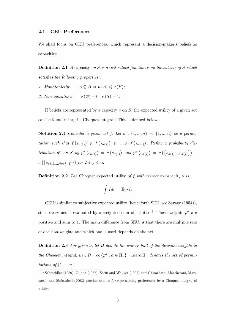
2.1 CEU Preferences

We shall focus on CEU preferences, which represent a decision-maker�s beliefs as

capacities.

De�nition 2.1 A capacity on S is a real-valued function � on the subsets of S which

satis�es the following properties:,

1. Monotonicity: A � B ) � (A) 6 � (B) ;

2. Normalisation: � (?) = 0; � (S) = 1:

If beliefs are represented by a capacity � on S, the expected utility of a given act

can be found using the Choquet integral. This is de�ned below.

Notation 2.1 Consider a given act f: Let � : f1; :::; ng ! f1; :::; ng be a permu-

tation such that f�s�(1)

�> f

�s�(2)

�> ::: > f

�s�(n)

�: De�ne a probability dis-

tribution p� on S by p��s�(1)

�= �

�s�(1)

�and p�

�s�(j)

�= �

��s�(1);:::;s�(j)

��

���s�(1);:::;s�(j�1)

�for 2 6 j 6 n:

De�nition 2.2 The Choquet expected utility of f with respect to capacity � is:Zfd� = Ep�f:

CEU is similar to subjective expected utility (henceforth SEU, see Savage (1954)),

since every act is evaluated by a weighted sum of utilities.2 These weights p� are

positive and sum to 1. The main di¤erence from SEU, is that there are multiple sets

of decision-weights and which one is used depends on the act.

De�nition 2.3 For given �; let D denote the convex hull of the decision weights in

the Choquet integral, i.e., D =co fp� : � 2 �ng ; where �n denotes the set of permu-

tations of f1; :::; ng :2Schmeidler (1989), Gilboa (1987), Sarin and Wakker (1992) and Ghirardato, Maccheroni, Mari-

nacci, and Siniscalchi (2003) provide axioms for representing preferences by a Choquet integral of

utility.

3

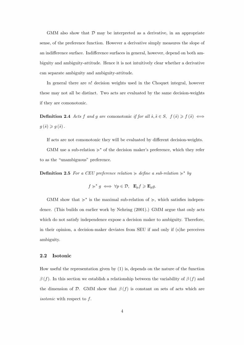
GMM also show that D may be interpreted as a derivative, in an appropriate

sense, of the preference function. However a derivative simply measures the slope of

an indi¤erence surface. Indi¤erence surfaces in general, however, depend on both am-

biguity and ambiguity-attitude. Hence it is not intuitively clear whether a derivative

can separate ambiguity and ambiguity-attitude.

In general there are n! decision weights used in the Choquet integral, however

these may not all be distinct. Two acts are evaluated by the same decision-weights

if they are comonotonic.

De�nition 2.4 Acts f and g are comonotonic if for all s; ~s 2 S; f (s) > f (~s) ()

g (s) > g (~s) :

If acts are not comonotonic they will be evaluated by di¤erent decision-weights.

GMM use a sub-relation <� of the decision maker�s preference, which they refer

to as the �unambiguous�preference.

De�nition 2.5 For a CEU preference relation < de�ne a sub-relation <� by

f <� g () 8p 2 D; Epf > Epg:

GMM show that <� is the maximal sub-relation of <; which satis�es indepen-

dence. (This builds on earlier work by Nehring (2001).) GMM argue that only acts

which do not satisfy independence expose a decision maker to ambiguity. Therefore,

in their opinion, a decision-maker deviates from SEU if and only if (s)he perceives

ambiguity.

2.2 Isotonic

How useful the representation given by (1) is, depends on the nature of the function

� (f). In this section we establish a relationship between the variability of � (f) and

the dimension of D. GMM show that � (f) is constant on sets of acts which are

isotonic with respect to f .

4

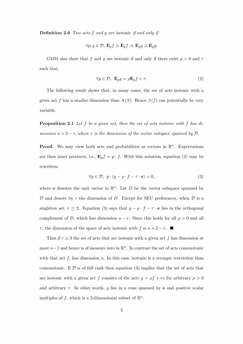
De�nition 2.6 Two acts f and g are isotonic if and only if

8p; q 2 D, Epf > Eqf ) Epg > Eqg.

GMM also show that f and g are isotonic if and only if there exist � > 0 and �

such that,

8p 2 D, Epg = �Epf + � . (2)

The following result shows that, in many cases, the set of acts isotonic with a

given act f has a smaller dimension than A (S). Hence � (f) can potentially be very

variable.

Proposition 2.1 Let f be a given act, then the set of acts isotonic with f has di-

mension n+ 2� r; where r is the dimension of the vector subspace spanned by D:

Proof. We may view both acts and probabilities as vectors in Rn. Expectations

are then inner products, i.e., Epf = p � f . With this notation, equation (2) may be

rewritten:

8p 2 D, p � (g � � � f � � � e) = 0, (3)

where e denotes the unit vector in Rn. Let D be the vector subspace spanned by

D and denote by r the dimension of D. Except for SEU preferences, when D is a

singleton set, r � 2. Equation (3) says that g � � � f � � � e lies in the orthogonal

complement of D, which has dimension n � r. Since this holds for all � > 0 and all

� , the dimension of the space of acts isotonic with f is n+ 2� r.

Thus if r > 3 the set of acts that are isotonic with a given act f has dimension at

most n�1 and hence is of measure zero in Rn. In contrast the set of acts comonotonic

with that act f , has dimension n. In this case, isotonic is a stronger restriction than

comonotonic. If D is of full rank then equation (3) implies that the set of acts that

are isotonic with a given act f consists of the acts g = �f + �e for arbitrary � > 0

and arbitrary � . In other words, g lies in a cone spanned by e and positive scalar

multiples of f , which is a 2-dimensional subset of Rn.

5

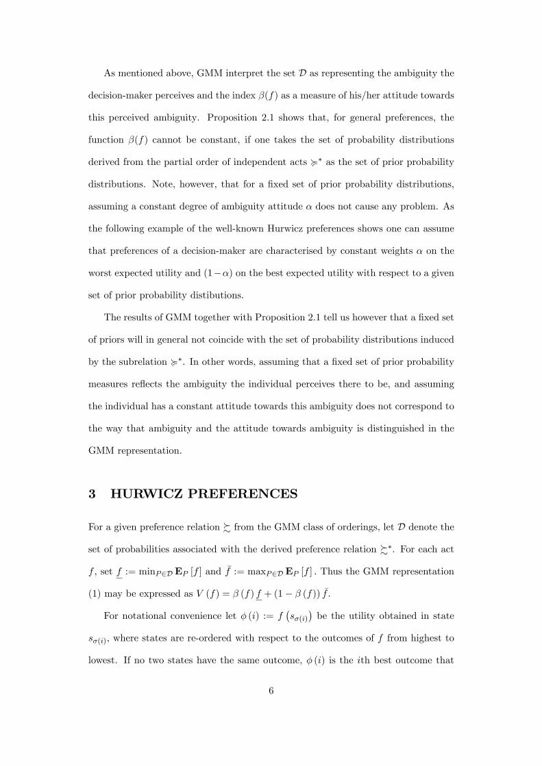
As mentioned above, GMM interpret the set D as representing the ambiguity the

decision-maker perceives and the index �(f) as a measure of his/her attitude towards

this perceived ambiguity. Proposition 2.1 shows that, for general preferences, the

function �(f) cannot be constant, if one takes the set of probability distributions

derived from the partial order of independent acts <� as the set of prior probability

distributions. Note, however, that for a �xed set of prior probability distributions,

assuming a constant degree of ambiguity attitude � does not cause any problem. As

the following example of the well-known Hurwicz preferences shows one can assume

that preferences of a decision-maker are characterised by constant weights � on the

worst expected utility and (1��) on the best expected utility with respect to a given

set of prior probability distibutions.

The results of GMM together with Proposition 2.1 tell us however that a �xed set

of priors will in general not coincide with the set of probability distributions induced

by the subrelation <�. In other words, assuming that a �xed set of prior probability

measures re�ects the ambiguity the individual perceives there to be, and assuming

the individual has a constant attitude towards this ambiguity does not correspond to

the way that ambiguity and the attitude towards ambiguity is distinguished in the

GMM representation.

3 HURWICZ PREFERENCES

For a given preference relation % from the GMM class of orderings, let D denote the

set of probabilities associated with the derived preference relation %�. For each act

f , set f := minP2D EP [f ] and �f := maxP2D EP [f ] : Thus the GMM representation

(1) may be expressed as V (f) = � (f) f + (1� � (f)) �f .

For notational convenience let � (i) := f�s�(i)

�be the utility obtained in state

s�(i); where states are re-ordered with respect to the outcomes of f from highest to

lowest. If no two states have the same outcome, � (i) is the ith best outcome that

6

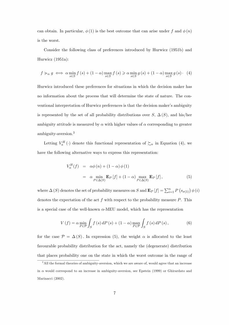
can obtain. In particular, � (1) is the best outcome that can arise under f and � (n)

is the worst.

Consider the following class of preferences introduced by Hurwicz (1951b) and

Hurwicz (1951a):

f <� g () �mins2S

f (s) + (1� �)maxs2S

f (s) > �mins2S

g (s) + (1� �)maxs2S

g (s) � (4)

Hurwicz introduced these preferences for situations in which the decision maker has

no information about the process that will determine the state of nature. The con-

ventional interpretation of Hurwicz preferences is that the decision maker�s ambiguity

is represented by the set of all probability distributions over S, �(S), and his/her

ambiguity attitude is measured by � with higher values of � corresponding to greater

ambiguity-aversion.3

Letting V Ha (�) denote this functional representation of %� in Equation (4), we

have the following alternative ways to express this representation:

V H� (f) = �� (n) + (1� �)� (1)

= � minP2�(S)

EP [f ] + (1� �) maxP2�(S)

EP [f ] , (5)

where�(S) denotes the set of probability measures on S andEP [f ] =Pni=1 P

�s�(1)

�� (i)

denotes the expectation of the act f with respect to the probability measure P . This

is a special case of the well-known �-MEU model, which has the representation

V (f) = �minP2P

ZSf (s) dP (s) + (1� �)max

P2P

ZSf (s) dP (s) , (6)

for the case P = �(S) : In expression (5), the weight � is allocated to the least

favourable probability distribution for the act, namely the (degenerate) distribution

that places probability one on the state in which the worst outcome in the range of

3All the formal theories of ambiguity-aversion, which we are aware of, would agree that an increase

in � would correspond to an increase in ambiguity-aversion, see Epstein (1999) or Ghirardato and

Marinacci (2002).

7

the act obtains (i.e. state s�(n) on which the outcome � (n) obtains). The remaining

weight (1� �) is allocated to the most favourable probability distribution for this

act, the (degenerate) distribution that places probability one on the state in which

the best outcome in the range of the act obtains (i.e. the state s�(1) on which the

outcome � (1) obtains).

The next result shows how GMM�s representation applies to Hurwicz preferences.

Proposition 3.1 If n > 3; Hurwicz preferences may be represented in the form given

by equation (1) provided:

1. D is the convex hull of the following set of n (n� 1) probability measures,

fP�st 2 �(S) , s; t 2 S; s 6= t : P�st (fsg) = �, P�st (ftg) = 1� �; P�st (f!g) = 0; ! 6= s; tg ;

2. � (f) =

8>>>>><>>>>>:

��(1��)(1� )�+(1��)� if � > 1=2;

� ��+(1��) if � < 1=2;

where = �(2)��(n)�(1)��(n) and � =

�(2)��(n�1)�(1)��(n) .

Proof. Since these preferences may be represented as a Choquet integral, the form

of the set D follows directly from GMM�s Example 17, which shows the set D is the

convex hull of the set of weights in the Choquet integral. Fix a non-constant act f

(that is, � (1) > � (n)). There are two cases to consider: when � is greater than or

equal to 1=2 and when � is less than 1=2.

1. Suppose � > 1=2. Then f = �� (n) + (1� �)� (n� 1) and �f = �� (1) +

(1� �)� (2) : To represent the preferences in the GMM form given in (1) we require,

� (f) f + (1� � (f)) �f

= � (f) [�� (n) + (1� �)� (n� 1)] + [1� � (f)] [�� (1) + (1� �)� (2)]

= �� (n) + (1� �)� (1) :

8

This yields

� (f) =� (� (1)� � (n))� (1� �) (� (1)� � (2))

� (� (1)� � (n)) + (1� �) (� (2)� � (n� 1))

=�� (1� �) (1� )�+ (1� �) � .

In particular, if � = 1=2, then we have � (f) = = (1 + �).

2. Suppose � < 1=2. Then f = (1� �)� (n)+�� (n� 1) and �f = (1� �)� (1)+

�� (2) : Now we require:

� (f) f + (1� � (f)) �f

= � (f) [(1� �)� (n) + �� (n� 1)] + [1� � (f)] [(1� �)� (1) + �� (2)]

= �� (n) + (1� �)� (1) ,

which yields

� (f) =� (� (2)� � (n))

� (� (2)� � (n� 1)) + (1� �) (� (1)� � (n))

=�

�� + (1� �) .

In �gure 1, we provide an illustration of the set D for the case of n = 3 and

� < 1=2.

9

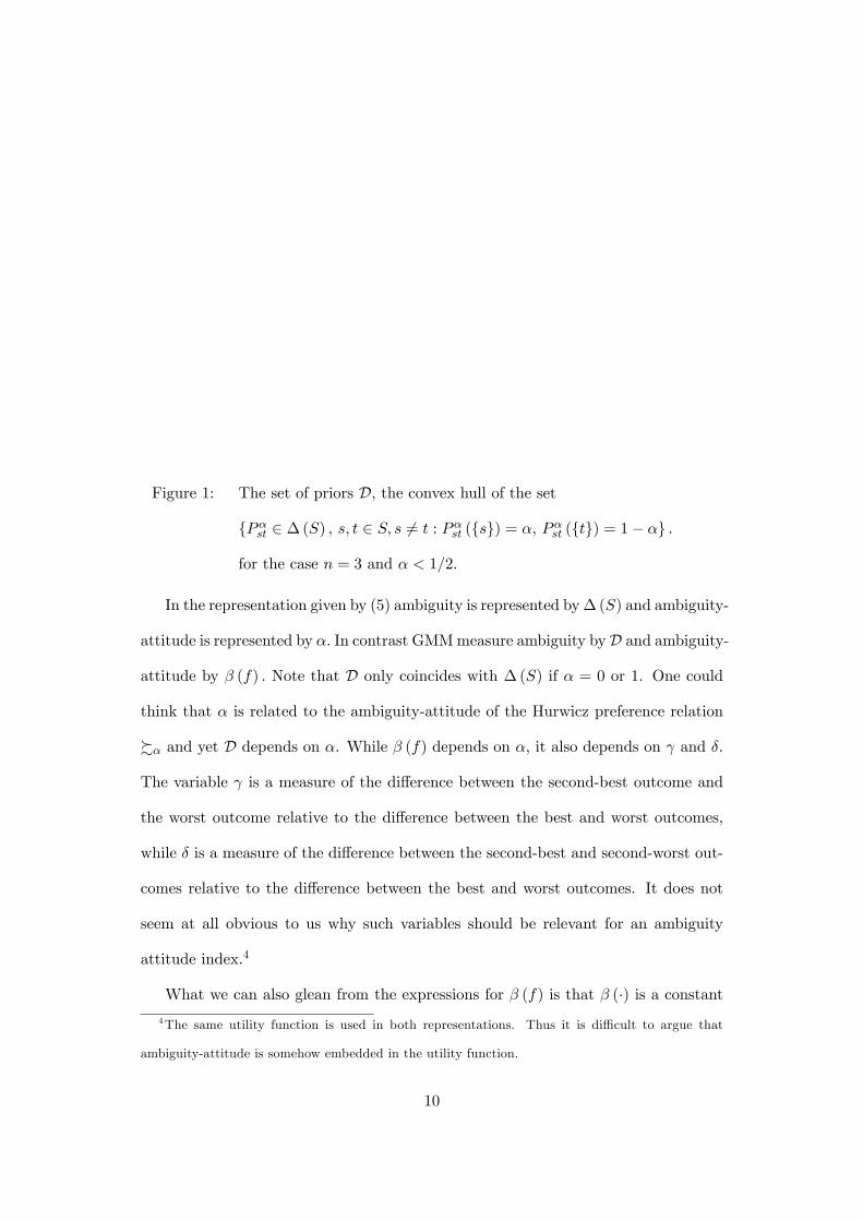
Figure 1: The set of priors D, the convex hull of the set

fP�st 2 �(S) , s; t 2 S; s 6= t : P�st (fsg) = �, P�st (ftg) = 1� �g .

for the case n = 3 and � < 1=2.

In the representation given by (5) ambiguity is represented by�(S) and ambiguity-

attitude is represented by �: In contrast GMMmeasure ambiguity byD and ambiguity-

attitude by � (f) : Note that D only coincides with �(S) if � = 0 or 1. One could

think that � is related to the ambiguity-attitude of the Hurwicz preference relation

%� and yet D depends on �. While � (f) depends on �, it also depends on and �.

The variable is a measure of the di¤erence between the second-best outcome and

the worst outcome relative to the di¤erence between the best and worst outcomes,

while � is a measure of the di¤erence between the second-best and second-worst out-

comes relative to the di¤erence between the best and worst outcomes. It does not

seem at all obvious to us why such variables should be relevant for an ambiguity

attitude index.4

What we can also glean from the expressions for � (f) is that � (�) is a constant4The same utility function is used in both representations. Thus it is di¢ cult to argue that

ambiguity-attitude is somehow embedded in the utility function.

10

function only if � = 1 or if � = 0. This means that if there are more than two

states then the only Hurwicz preference relations that satisfy GMM�s axiom 7 are

%1 and %0, that is, the cases of extreme pessimism and extreme optimism. This

is true more generally. In Eichberger, Grant, and Kelsey (2006) we show a similar

result applies to all �-MEU preferences, provided D consists of countably additive

probability distributions.

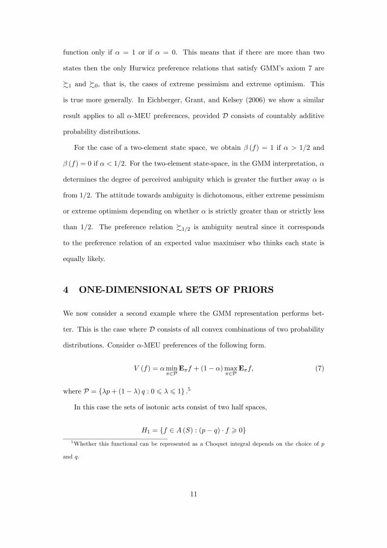
For the case of a two-element state space, we obtain � (f) = 1 if � > 1=2 and

� (f) = 0 if � < 1=2. For the two-element state-space, in the GMM interpretation, �

determines the degree of perceived ambiguity which is greater the further away � is

from 1=2. The attitude towards ambiguity is dichotomous, either extreme pessimism

or extreme optimism depending on whether � is strictly greater than or strictly less

than 1=2. The preference relation %1=2 is ambiguity neutral since it corresponds

to the preference relation of an expected value maximiser who thinks each state is

equally likely.

4 ONE-DIMENSIONAL SETS OF PRIORS

We now consider a second example where the GMM representation performs bet-

ter. This is the case where D consists of all convex combinations of two probability

distributions. Consider �-MEU preferences of the following form.

V (f) = �min�2P

E�f + (1� �)max�2P

E�f; (7)

where P = f�p+ (1� �) q : 0 6 � 6 1g :5

In this case the sets of isotonic acts consist of two half spaces,

H1 = ff 2 A (S) : (p� q) � f > 0g5Whether this functional can be represented as a Choquet integral depends on the choice of p

and q:

11

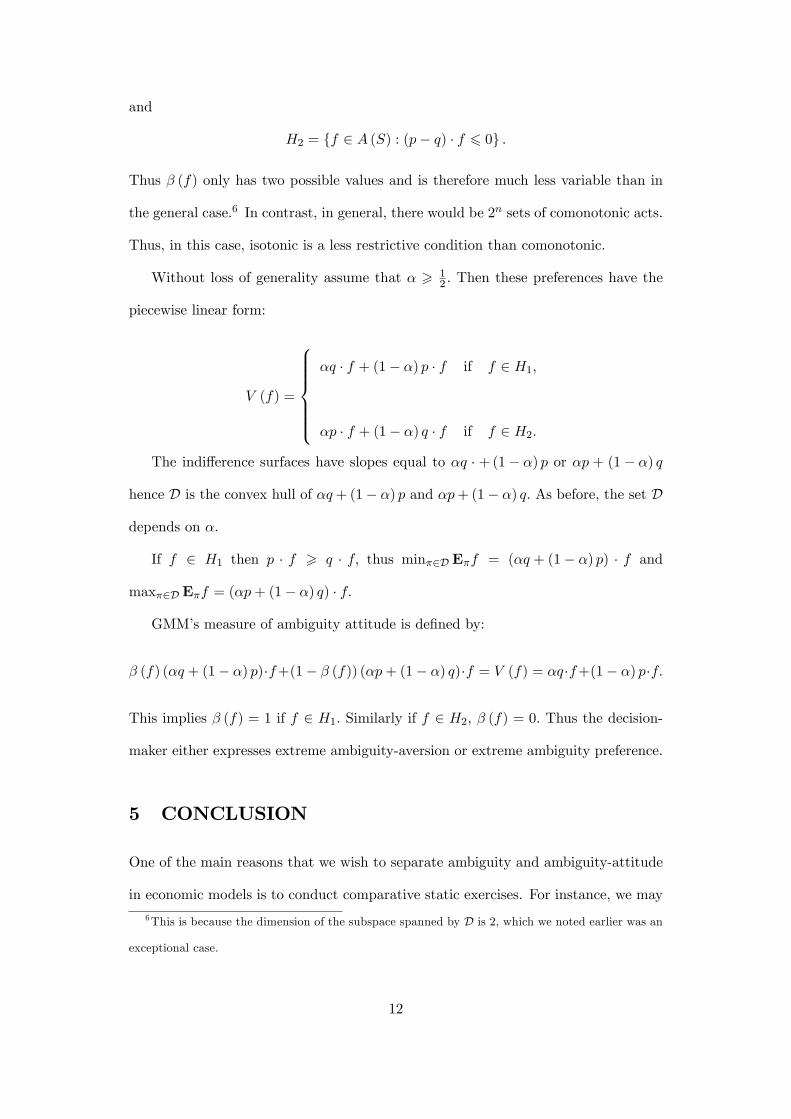
and

H2 = ff 2 A (S) : (p� q) � f 6 0g :

Thus � (f) only has two possible values and is therefore much less variable than in

the general case.6 In contrast, in general, there would be 2n sets of comonotonic acts.

Thus, in this case, isotonic is a less restrictive condition than comonotonic.

Without loss of generality assume that � > 12 : Then these preferences have the

piecewise linear form:

V (f) =

8>>>>><>>>>>:�q � f + (1� �) p � f if f 2 H1;

�p � f + (1� �) q � f if f 2 H2:

The indi¤erence surfaces have slopes equal to �q � +(1� �) p or �p + (1� �) q

hence D is the convex hull of �q + (1� �) p and �p+ (1� �) q: As before, the set D

depends on �:

If f 2 H1 then p � f > q � f; thus min�2D E�f = (�q + (1� �) p) � f and

max�2D E�f = (�p+ (1� �) q) � f:

GMM�s measure of ambiguity attitude is de�ned by:

� (f) (�q + (1� �) p)�f+(1� � (f)) (�p+ (1� �) q)�f = V (f) = �q�f+(1� �) p�f:

This implies � (f) = 1 if f 2 H1: Similarly if f 2 H2, � (f) = 0: Thus the decision-

maker either expresses extreme ambiguity-aversion or extreme ambiguity preference.

5 CONCLUSION

One of the main reasons that we wish to separate ambiguity and ambiguity-attitude

in economic models is to conduct comparative static exercises. For instance, we may

6This is because the dimension of the subspace spanned by D is 2, which we noted earlier was an

exceptional case.

12

wish to �nd the e¤ect of varying ambiguity-attitude while keeping ambiguity constant.

Doing such comparative static analysis GMM�s framework, where ambiguity and

ambiguity-attitude are simultaneously determined, is not completely straightforward.

This expository note uses some examples to illustrate the implications of GMM�s

axioms 1-5. In Eichberger, Grant, and Kelsey (2006) we show that the only pref-

erences which satisfy their axioms 1-5 plus 7 are the two extreme cases MEU or

maxmax expected utility.

References

Arrow, K., and L. Hurwicz (1972): �An Optimality Criterion for Decision Making

under Ignorance,� in Uncertainty and Expectations in Economics, ed. by C. F.

Carter, and J. Ford. Blackwell, Oxford.

Eichberger, J., S. Grant, and D. Kelsey (2006): �Di¤erentiating Ambiguity:

A Comment,�University of Exeter, working paper, 06/06.

Epstein, L. G. (1999): �A De�nition of Uncertainty Aversion,�Review of Economic

Studies, 66, 579�606.

Ghirardato, P., F. Maccheroni, and M. Marinacci (2004): �Di¤erentiating

Ambiguity and Ambiguity Attitude,�Journal of Economic Theory, 118, 133�173.

Ghirardato, P., F. Maccheroni, M. Marinacci, and M. Siniscalchi (2003):

�A Subjective Spin on Roulette Wheels,�Econometrica, 71, 1897�1908.

Ghirardato, P., and M. Marinacci (2002): �Ambiguity Made Precise: A Com-

parative Foundation,�Journal of Economic Theory, 102, 251�289.

Gilboa, I. (1987): �Expected Utility with Purely Subjective Non-additive Proba-

bilities,�Journal of Mathematical Economics, 16, 65�88.

13

Hurwicz, L. (1951a): �Optimiality Criteria for Decision Making under Ignorance,�

Discussion paper 370, Cowles Comission.

Hurwicz, L. (1951b): �Some Speci�cation Problems and Application to Econometric

Models,�Econometrica, 19, 343�344.

Nehring, K. (2001): �Decision-Making in the Context of Imprecise Probabilitistic

Beliefs,�working paper, University of California, Davis.

Sarin, R., and P. Wakker (1992): �A Simple Axiomatization of Non-Additive

Expected Utility,�Econometrica, 60, 1255�1272.

Savage, L. J. (1954): Foundations of Statistics. Wiley, New York.

Schmeidler, D. (1989): �Subjective Probability and Expected Utility without Ad-

ditivity,�Econometrica, 57, 571�587.

14