Disconnected Skeleton: Shape at its Absolute

Scale

C. Aslan, A. Erdem, E. Erdem and S. Tari

Abstract

We present a new skeletal representation along with a matching framework to address the deformable

shape recognition problem. The disconnectedness arises as a result of excessive regularization that we

use to describe a shape at an attainably coarse scale. Our motivation is to rely on the stable properties

of the shape instead of inaccurately measured secondary details. The new representation does not suffer

from the common instability problems of traditional connected skeletons, and the matching process

gives quite successful results on a diverse database of 2D shapes. An important difference of our

approach from the conventional use of the skeleton is that we replace the local coordinate frame with a

global Euclidean frame supported by additional mechanisms to handle articulations and local boundary

deformations. As a result, we can produce descriptions that are sensitive to any combination of changes

in scale, position, orientation and articulation, as well as invariant ones.

Index Terms

skeleton, shape representation, object centered coordinate frame, diffusion equation

NOTES

The work excluding §V and §VI has first appeared in 2005 [2], [4]:

• Aslan, C., Tari, S.: An Axis-Based Representation for Recognition. In ICCV(2005) 1339-

1346.

• Aslan, C., : Disconnected Skeletons for Shape Recognition. Masters thesis, Department of

Computer Engineering, Middle East Technical University, May 2005.

Corresponding authors: Sibel Tari (stari@metu.edu.tr) and Cagri Aslan (caslan@microsoft.com)

arX

iv:1

104.

2751

v1 [

cs.C

V]

14

Apr

201

1

T-PAMI vol. 30 no. 12, pp. 2188-2203, 2008

I. INTRODUCTION

Local symmetry axis based representations, commonly referred to as shape skeletons, have

been used in generic shape representation since the pioneering work of Blum [10] on the study

of form via axis morphology. The strength of axis based representations lies in expressing the

links among shape primitives and providing a shape centered coordinate frame.

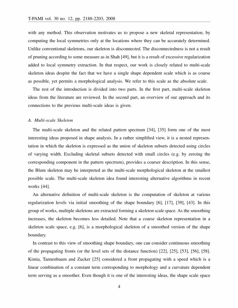
Blum’s skeleton can be explained using three alternative constructions. The original one is to

initiate fire fronts at time t = 0 along all the points of the shape boundary, and to let these fronts

propagate as wavefronts toward the center of the shape at uniform speed (Fig. 1(a)). The locus

of shock points, where these wavefronts would intersect and extinguish, defines the skeleton. An

important property of the skeleton is its ability to reconstruct the shape boundary by propagating

the wavefronts backwards. The second construction replaces the dynamic view of propagating

fronts with a static view by embedding time dependent wavefronts as the level curves of a surface

whose value at each point is the minimum distance of the point to the boundary (Fig. 1(b)).

Skeleton points are the ones which are equidistant from at least two boundary points. They

coincide with the shock points. They are the sharp points of the level curves of the distance

function. It is possible to detect these points by projecting the ridges of the distance function

on the shape plane. The third construction is via maximal circles that are inscribable inside the

shape and touch the shape boundary at more than one point. In this construction, circle radius

plays the role of time of arrival in the symmetry axis function. Considering the envelope of

maximal circles, one can reconstruct the shape boundary (Fig. 1(c)).

Independent of Blum’s morphological analysis, mathematical morphology has been developed

as a set theoretic approach to shape [36], [46]. Following Lantuejoul’s work [28] which showed

that the skeleton can be constructed by set transformations, a significant amount of skeletonization

work developed within the mathematical morphology community. Basic set transformations that

are applied to shapes with the help of structuring elements are called erosions and dilations

(Fig. 1(d)). Note that when the structuring element is chosen as a disk of diameter d, the eroded

shape boundary becomes equivalent to the wave front at t = d. Eroding the shape first and

dilating it later with the disk structuring element removes the sharp corners which correspond

to the shock points of the wave model.

While all of these constructions lead to the same representation, they inspired many others

2

T-PAMI vol. 30 no. 12, pp. 2188-2203, 2008

(a) (b) (c) (d)

Fig. 1. Construction of the skeleton for a rectangle. (a) grass-fire method. (b) distance transform. (c) maximal circles. (d)

erosions and dilations with a disc as the structuring element. Dashed lines are the transformed versions of solid lines.

having different properties and being computed with different algorithms, e.g. [12], [13], [20],

[23], [26], [27], [31], [32], [35], [39], [44], [52], [58], [60], [61]. There is a connection between

positive curvature maxima of the shape boundary and the skeleton in the sense that each curvature

maximum gives rise to a skeletal branch [32]. This connection is often used to extract the

skeleton. When the skeleton is extended to include branches that arise from curvature minima,

a richer set commonly referred to as local symmetry axes is obtained [12]. Note that the term

symmetry as used in this context is different than conventional symmetry and is a property of

points generated by the shape rather than being a property of shapes themselves [10], [56].

A major reason for having alternative skeleton constructions is that the skeleton is an unstable

representation in the sense that a small change in the shape may cause a significant change in

its description. Difficulties associated with a robust implementation are the major source of a

significant body of research dedicated to regularization and richer definitions of local symmetry.

Even though there are interesting ideas in recent works [20], [52], [60], pruning of the axes

has been mostly used to simplify or regularize the skeleton. In general, pruning methods define

a saliency measure for the axis points and discard those points whose significance is below a

threshold. Axis length, propagation velocity, maximal thickness, and the ratio of the axis to the

boundary it unfolds are the most typical significance measures; however, they do not necessarily

reflect the perceptual prominence of parts [51].

Interestingly, – as also observed in [5], [49], [59], [60] – while the accurate computation of the

skeleton branches corresponding to noise and secondary details is difficult, the ones correspond-

ing to ribbon-like parts of the shape with slowly varying width can be accurately determined

3

T-PAMI vol. 30 no. 12, pp. 2188-2203, 2008

with any method. This observation motivates us to propose a new skeletal representation, by

computing the local symmetries only at the locations where they can be accurately determined.

Unlike conventional skeletons, our skeleton is disconnected. The disconnectedness is not a result

of pruning according to some measure as in Shah [49], but it is a result of excessive regularization

added to local symmetry extraction. In that respect, our work is closely related to multi-scale

skeleton ideas despite the fact that we have a single shape dependent scale which is as coarse

as possible, yet permits a morphological analysis. We refer to this scale as the absolute scale.

The rest of the introduction is divided into two parts. In the first part, multi-scale skeleton

ideas from the literature are reviewed. In the second part, an overview of our approach and its

connections to the previous multi-scale ideas is given.

A. Multi-scale Skeleton

The multi-scale skeleton and the related pattern spectrum [34], [35] form one of the most

interesting ideas proposed in shape analysis. In a rather simplified view, it is a nested represen-

tation in which the skeleton is expressed as the union of skeleton subsets detected using circles

of varying width. Excluding skeletal subsets detected with small circles (e.g. by zeroing the

corresponding component in the pattern spectrum), provides a coarser description. In this sense,

the Blum skeleton may be interpreted as the multi-scale morphological skeleton at the smallest

possible scale. The multi-scale skeleton idea found interesting alternative algorithms in recent

works [44].

An alternative definition of multi-scale skeleton is the computation of skeleton at various

regularization levels via initial smoothing of the shape boundary [6], [17], [39], [43]. In this

group of works, multiple skeletons are extracted forming a skeleton scale space. As the smoothing

increases, the skeleton becomes less detailed. Note that a coarse skeleton representation in a

skeleton scale space, e.g. [6], is a morphological skeleton of a smoothed version of the shape

boundary.

In contrast to this view of smoothing shape boundary, one can consider continuous smoothing

of the propagating fronts (or the level sets of the distance function) [22], [25], [53], [56], [58].

Kimia, Tannenbaum and Zucker [25] considered a front propagating with a speed which is a

linear combination of a constant term corresponding to morphology and a curvature dependent

term serving as a smoother. Even though it is one of the interesting ideas, the shape scale space

4

T-PAMI vol. 30 no. 12, pp. 2188-2203, 2008

obtained via this model has not been used in shape recognition. In the shock-loci methods,

Kimia et al. switched to the use of constant speed corresponding to morphology [44]. One

reason is that the speed function taking negative values poses computational difficulties. Another

difficulty is that due to smoothing, shock points turn into high curvature points which are harder

to detect accurately. Computational difficulties could be alleviated by considering a speed which

is positive everywhere as demonstrated by Tari, Shah and Pien (TSP) [57], [58] and Gorelick et

al. [22]. In these alternative frameworks, one obtains an analogue of the smoothed distance

surface via solving elliptic PDEs. The solution can be related to the wave model by considering

a propagation speed which is an increasing function of medialness. In the TSP method, time of

arrival is approximately a decaying exponential function of distance from the shape boundary.

Skeletal points moving with a faster speed than the non-skeletal points can be detected by the

minima of the gradient which are indirectly related to curvature maxima.

B. Our Approach

Our approach to compute the symmetry set (described in Section II) is directly related to that

of TSP [57], [58]. Our major departure is to let the regularization tend to infinity and dominate

over morphology. To achieve this, we propose a special surface φ taking values in (0, 1] and

whose 1- level curve corresponds to the shape boundary and other level curves roughly mimic

the evolution of the boundary towards a circle. In a naive sense, the surface φ is the limit of the

surface in TSP when the smoothing tends to infinity. The level curves of φ can be interpreted

as multi-scale erosions with non-homogeneous structuring elements: ellipses of varying aspect

ratio and size. The local symmetry points corresponding to the curvature extrema of the evolving

boundary (note that these are smoothed shock points) end as soon as the evolving curve locally

becomes a circle. For this reason, unlike the conventional skeleton, ours is not connected.

The disconnection points have an interesting interpretation in terms of the connected morpho-

logical skeleton. In the traditional construction, the angle between two symmetry-shape geodesics

(shortest distance from axis point to boundary) gives the object angle [10]. On one hand, at

regions of slowly varying width, this angle is large. On the other hand, it is small near branch

points where the skeleton computation is sensitive to noise and secondary details. As such, the

disconnected axes are analogous to pruned skeletons using object angle or its variants [49].

5

T-PAMI vol. 30 no. 12, pp. 2188-2203, 2008

We remark that the connection of our approach to multi-scale skeleton ideas is rather counter-

intuitive. In comparison to the definition by Maragos [34], [35], our skeleton representation is

roughly high-passed where the skeletal subsets detected with circles of larger radius are filtered

out. In contrast to skeleton scale space methods which smooth the boundary first and then

compute the skeleton, we, in a dynamic way, continuously smooth the shape boundary and

record its special points till the whole boundary becomes simple enough to admit any. Unlike

in skeleton scale space representation, we do not form a hierarchy of skeletons. We have just

a single skeleton computed at the coarsest possible scale in which a skeletal description is still

possible.

The disconnected axes corresponding to ribbon-like sections (or equivalently isolated simple

symmetry branches) form the primitives of our representation. Each primitive is described by

its disconnection location and its length. As such, the proposed representation is an unlabeled

attributed point set and forms a trade-off between unstructured point sets, e.g. [9], [14], [16] and

skeletal graphs, e.g. [20], [45], [54], [61].

A strong motivation for computing a skeleton is to define a shape centered coordinate frame

in order to cope with visual transformations. Blum [10] defined this frame as a local affine frame

defined by three parameters: symmetry axis curvature, width and width angle. Such a local frame

is utilized in recent appearance based recognition work [40]. However, when a skeleton becomes

disconnected due to excessive smoothing, the local coordinate frame in a large central area is lost.

As a solution, we propose to separate visual changes into three groups; as rigid transformations,

piecewise rigid transformations (articulations) and infinitesimal transformations (deformations).

We develop a global Euclidean frame (Section III) and demonstrate that the coarse spatial

structure imposed by this frame is sufficient for shape comparison in a way which is robust to

articulations as well as Euclidean transformations (Section IV). Even though invariance to visual

transformations is desirable, there are situations in which transformation variant descriptors must

be used, e.g. discriminating ‘6’ from ‘9’ or discriminating a likely articulation from an unlikely

one (Fig. 2). To introduce sensitivity to articulations we propose a part-centered coordinate frame

(Section V). Finally, to handle deformations we resort to the techniques developed for landmark

point based representations [11], [24] (Section VI). By separating visual transformations, we

can produce descriptions that are sensitive to any combination of changes in scale, location,

orientation, and articulations in addition to descriptions that are invariant to these changes.

6

T-PAMI vol. 30 no. 12, pp. 2188-2203, 2008

The hybrid (axis vs. point) nature of our local symmetry representation makes the necessary

constructions and computations almost trivial.

A preliminary conference version of this work appeared in [4]. Implementation details are

provided in the supplementary material [3].

(a) (b) (c) (d)

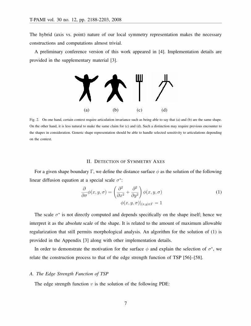
Fig. 2. On one hand, certain context require articulation invariance such as being able to say that (a) and (b) are the same shape.

On the other hand, it is less natural to make the same claim for (c) and (d). Such a distinction may require previous encounter to

the shapes in consideration. Generic shape representation should be able to handle selected sensitivity to articulations depending

on the context.

II. DETECTION OF SYMMETRY AXES

For a given shape boundary Γ, we define the distance surface φ as the solution of the following

linear diffusion equation at a special scale σ∗:

∂

∂σφ(x, y, σ) =

(∂2

∂x2+

∂2

∂y2

)φ(x, y, σ) (1)

φ(x, y, σ)|(x,y)∈Γ = 1

The scale σ∗ is not directly computed and depends specifically on the shape itself; hence we

interpret it as the absolute scale of the shape. It is related to the amount of maximum allowable

regularization that still permits morphological analysis. An algorithm for the solution of (1) is

provided in the Appendix [3] along with other implementation details.

In order to demonstrate the motivation for the surface φ and explain the selection of σ∗, we

relate the construction process to that of the edge strength function of TSP [56]–[58].

A. The Edge Strength Function of TSP

The edge strength function v is the solution of the following PDE:

7

T-PAMI vol. 30 no. 12, pp. 2188-2203, 2008

(∂2

∂x2+

∂2

∂y2

)v(x, y)− v(x, y)

ρ2= 0 (2)

v(x, y)|(x,y)∈Γ = 1

The function v attains its highest value of 1 at the shape boundary Γ, and decays monotonically

as a function of the distance from the boundary. As such, it is a smoothed analogue of the distance

function. Solution of (2) can also be expressed as the steady-state solution of a linear diffusion

equation with a bias term:

∂

∂σv(x, y, σ) =

(∂2

∂x2+

∂2

∂y2

)v(x, y, σ)− v(x, y, σ)

ρ2(3)

v(x, y)|(x,y)∈Γ = 1

As the only parameter ρ approaches to zero, v function becomes an approximation of the

discontinuity locus of the Mumford-Shah segmentation model [1], [38], [47], [48]. For larger ρ

values (e.g. 4, 8, 16), the edge strength function acts like a level set function whose level curves

mimic the propagation of the shape boundary in the inward normal direction with a curvature

dependent velocity [56]–[58], as in the curve evolution of Kimia, Tannenbaum and Zucker [25].

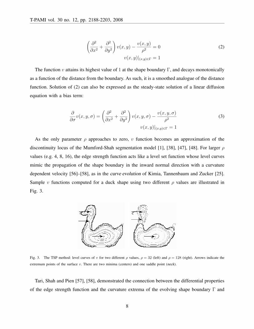
Sample v functions computed for a duck shape using two different ρ values are illustrated in

Fig. 3.

Fig. 3. The TSP method: level curves of v for two different ρ values, ρ = 32 (left) and ρ = 128 (right). Arrows indicate the

extremum points of the surface v. There are two minima (centers) and one saddle point (neck).

Tari, Shah and Pien [57], [58], demonstrated the connection between the differential properties

of the edge strength function and the curvature extrema of the evolving shape boundary Γ and

8

T-PAMI vol. 30 no. 12, pp. 2188-2203, 2008

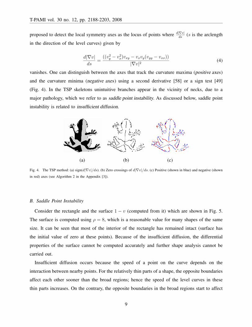
proposed to detect the local symmetry axes as the locus of points where d|∇v|ds

(s is the arclength

in the direction of the level curves) given by

d|∇v|ds

=((v2

y − v2x)vxy − vxvy(vyy − vxx))

|∇v|2(4)

vanishes. One can distinguish between the axes that track the curvature maxima (positive axes)

and the curvature minima (negative axes) using a second derivative [58] or a sign test [49]

(Fig. 4). In the TSP skeletons unintuitive branches appear in the vicinity of necks, due to a

major pathology, which we refer to as saddle point instability. As discussed below, saddle point

instability is related to insufficient diffusion.

(a) (b) (c)

Fig. 4. The TSP method: (a) sign(d|∇v|/ds). (b) Zero crossings of d|∇v|/ds. (c) Positive (shown in blue) and negative (shown

in red) axes (see Algorithm 2 in the Appendix [3]).

B. Saddle Point Instability

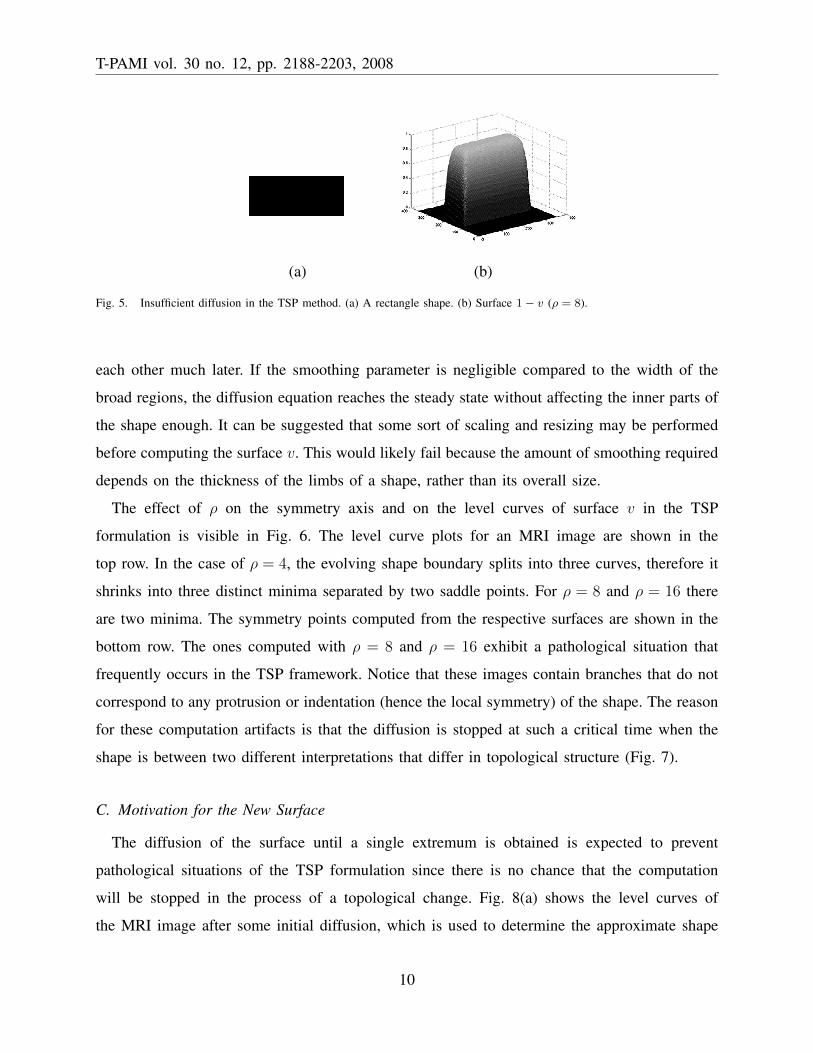
Consider the rectangle and the surface 1− v (computed from it) which are shown in Fig. 5.

The surface is computed using ρ = 8, which is a reasonable value for many shapes of the same

size. It can be seen that most of the interior of the rectangle has remained intact (surface has

the initial value of zero at these points). Because of the insufficient diffusion, the differential

properties of the surface cannot be computed accurately and further shape analysis cannot be

carried out.

Insufficient diffusion occurs because the speed of a point on the curve depends on the

interaction between nearby points. For the relatively thin parts of a shape, the opposite boundaries

affect each other sooner than the broad regions; hence the speed of the level curves in these

thin parts increases. On the contrary, the opposite boundaries in the broad regions start to affect

9

T-PAMI vol. 30 no. 12, pp. 2188-2203, 2008

(a) (b)

Fig. 5. Insufficient diffusion in the TSP method. (a) A rectangle shape. (b) Surface 1− v (ρ = 8).

each other much later. If the smoothing parameter is negligible compared to the width of the

broad regions, the diffusion equation reaches the steady state without affecting the inner parts of

the shape enough. It can be suggested that some sort of scaling and resizing may be performed

before computing the surface v. This would likely fail because the amount of smoothing required

depends on the thickness of the limbs of a shape, rather than its overall size.

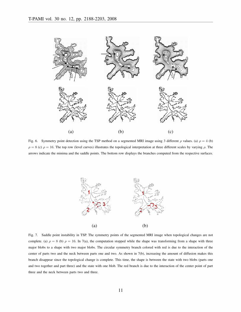
The effect of ρ on the symmetry axis and on the level curves of surface v in the TSP

formulation is visible in Fig. 6. The level curve plots for an MRI image are shown in the

top row. In the case of ρ = 4, the evolving shape boundary splits into three curves, therefore it

shrinks into three distinct minima separated by two saddle points. For ρ = 8 and ρ = 16 there

are two minima. The symmetry points computed from the respective surfaces are shown in the

bottom row. The ones computed with ρ = 8 and ρ = 16 exhibit a pathological situation that

frequently occurs in the TSP framework. Notice that these images contain branches that do not

correspond to any protrusion or indentation (hence the local symmetry) of the shape. The reason

for these computation artifacts is that the diffusion is stopped at such a critical time when the

shape is between two different interpretations that differ in topological structure (Fig. 7).

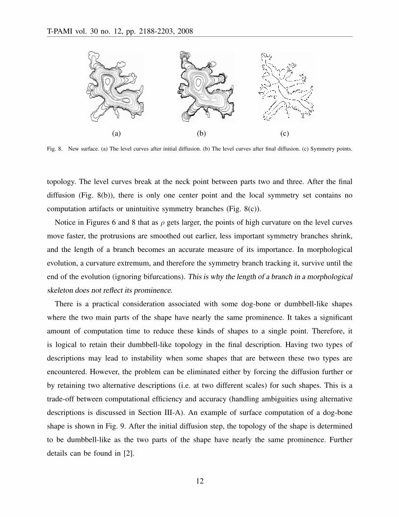
C. Motivation for the New Surface

The diffusion of the surface until a single extremum is obtained is expected to prevent

pathological situations of the TSP formulation since there is no chance that the computation

will be stopped in the process of a topological change. Fig. 8(a) shows the level curves of

the MRI image after some initial diffusion, which is used to determine the approximate shape

10

T-PAMI vol. 30 no. 12, pp. 2188-2203, 2008

(a) (b) (c)

Fig. 6. Symmetry point detection using the TSP method on a segmented MRI image using 3 different ρ values. (a) ρ = 4 (b)

ρ = 8 (c) ρ = 16. The top row (level curves) illustrates the topological interpretation at three different scales by varying ρ. The

arrows indicate the minima and the saddle points. The bottom row displays the branches computed from the respective surfaces.

(a) (b)

Fig. 7. Saddle point instability in TSP. The symmetry points of the segmented MRI image when topological changes are not

complete. (a) ρ = 8 (b) ρ = 16. In 7(a), the computation stopped while the shape was transforming from a shape with three

major blobs to a shape with two major blobs. The circular symmetry branch colored with red is due to the interaction of the

center of parts two and the neck between parts one and two. As shown in 7(b), increasing the amount of diffusion makes this

branch disappear since the topological change is complete. This time, the shape is between the state with two blobs (parts one

and two together and part three) and the state with one blob. The red branch is due to the interaction of the center point of part

three and the neck between parts two and three.

11

T-PAMI vol. 30 no. 12, pp. 2188-2203, 2008

(a) (b) (c)

Fig. 8. New surface. (a) The level curves after initial diffusion. (b) The level curves after final diffusion. (c) Symmetry points.

topology. The level curves break at the neck point between parts two and three. After the final

diffusion (Fig. 8(b)), there is only one center point and the local symmetry set contains no

computation artifacts or unintuitive symmetry branches (Fig. 8(c)).

Notice in Figures 6 and 8 that as ρ gets larger, the points of high curvature on the level curves

move faster, the protrusions are smoothed out earlier, less important symmetry branches shrink,

and the length of a branch becomes an accurate measure of its importance. In morphological

evolution, a curvature extremum, and therefore the symmetry branch tracking it, survive until the

end of the evolution (ignoring bifurcations). This is why the length of a branch in a morphological

skeleton does not reflect its prominence.

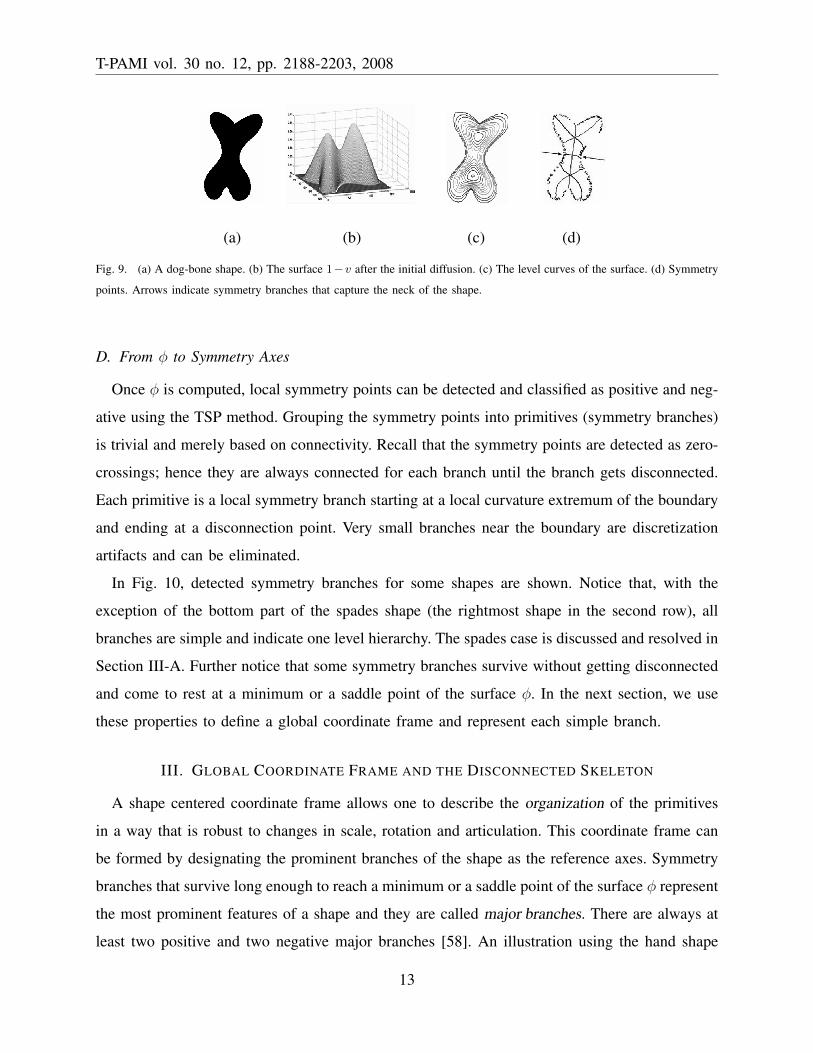
There is a practical consideration associated with some dog-bone or dumbbell-like shapes

where the two main parts of the shape have nearly the same prominence. It takes a significant

amount of computation time to reduce these kinds of shapes to a single point. Therefore, it

is logical to retain their dumbbell-like topology in the final description. Having two types of

descriptions may lead to instability when some shapes that are between these two types are

encountered. However, the problem can be eliminated either by forcing the diffusion further or

by retaining two alternative descriptions (i.e. at two different scales) for such shapes. This is a

trade-off between computational efficiency and accuracy (handling ambiguities using alternative

descriptions is discussed in Section III-A). An example of surface computation of a dog-bone

shape is shown in Fig. 9. After the initial diffusion step, the topology of the shape is determined

to be dumbbell-like as the two parts of the shape have nearly the same prominence. Further

details can be found in [2].

12

T-PAMI vol. 30 no. 12, pp. 2188-2203, 2008

(a) (b) (c) (d)

Fig. 9. (a) A dog-bone shape. (b) The surface 1−v after the initial diffusion. (c) The level curves of the surface. (d) Symmetry

points. Arrows indicate symmetry branches that capture the neck of the shape.

D. From φ to Symmetry Axes

Once φ is computed, local symmetry points can be detected and classified as positive and neg-

ative using the TSP method. Grouping the symmetry points into primitives (symmetry branches)

is trivial and merely based on connectivity. Recall that the symmetry points are detected as zero-

crossings; hence they are always connected for each branch until the branch gets disconnected.

Each primitive is a local symmetry branch starting at a local curvature extremum of the boundary

and ending at a disconnection point. Very small branches near the boundary are discretization

artifacts and can be eliminated.

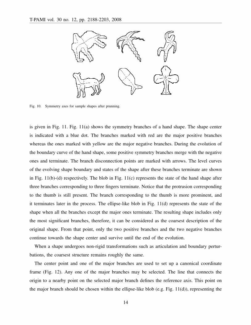
In Fig. 10, detected symmetry branches for some shapes are shown. Notice that, with the

exception of the bottom part of the spades shape (the rightmost shape in the second row), all

branches are simple and indicate one level hierarchy. The spades case is discussed and resolved in

Section III-A. Further notice that some symmetry branches survive without getting disconnected

and come to rest at a minimum or a saddle point of the surface φ. In the next section, we use

these properties to define a global coordinate frame and represent each simple branch.

III. GLOBAL COORDINATE FRAME AND THE DISCONNECTED SKELETON

A shape centered coordinate frame allows one to describe the organization of the primitives

in a way that is robust to changes in scale, rotation and articulation. This coordinate frame can

be formed by designating the prominent branches of the shape as the reference axes. Symmetry

branches that survive long enough to reach a minimum or a saddle point of the surface φ represent

the most prominent features of a shape and they are called major branches. There are always at

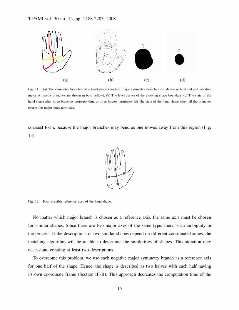
least two positive and two negative major branches [58]. An illustration using the hand shape

13

T-PAMI vol. 30 no. 12, pp. 2188-2203, 2008

Fig. 10. Symmetry axes for sample shapes after prunning.

is given in Fig. 11. Fig. 11(a) shows the symmetry branches of a hand shape. The shape center

is indicated with a blue dot. The branches marked with red are the major positive branches

whereas the ones marked with yellow are the major negative branches. During the evolution of

the boundary curve of the hand shape, some positive symmetry branches merge with the negative

ones and terminate. The branch disconnection points are marked with arrows. The level curves

of the evolving shape boundary and states of the shape after these branches terminate are shown

in Fig. 11(b)-(d) respectively. The blob in Fig. 11(c) represents the state of the hand shape after

three branches corresponding to three fingers terminate. Notice that the protrusion corresponding

to the thumb is still present. The branch corresponding to the thumb is more prominent, and

it terminates later in the process. The ellipse-like blob in Fig. 11(d) represents the state of the

shape when all the branches except the major ones terminate. The resulting shape includes only

the most significant branches, therefore, it can be considered as the coarsest description of the

original shape. From that point, only the two positive branches and the two negative branches

continue towards the shape center and survive until the end of the evolution.

When a shape undergoes non-rigid transformations such as articulation and boundary pertur-

bations, the coarsest structure remains roughly the same.

The center point and one of the major branches are used to set up a canonical coordinate

frame (Fig. 12). Any one of the major branches may be selected. The line that connects the

origin to a nearby point on the selected major branch defines the reference axis. This point on

the major branch should be chosen within the ellipse-like blob (e.g. Fig. 11(d)), representing the

14

T-PAMI vol. 30 no. 12, pp. 2188-2203, 2008

(a) (b) (c) (d)

Fig. 11. (a) The symmetry branches of a hand shape (positive major symmetry branches are shown in bold red and negative

major symmetry branches are shown in bold yellow). (b) The level curves of the evolving shape boundary. (c) The state of the

hand shape after three branches corresponding to three fingers terminate. (d) The state of the hand shape when all the branches

except the major ones terminate.

coarsest form, because the major branches may bend as one moves away from this region (Fig.

13).

Fig. 12. Four possible reference axes of the hand shape.

No matter which major branch is chosen as a reference axis, the same axis must be chosen

for similar shapes. Since there are two major axes of the same type, there is an ambiguity in

the process. If the descriptions of two similar shapes depend on different coordinate frames, the

matching algorithm will be unable to determine the similarities of shapes. This situation may

necessitate creating at least two descriptions.

To overcome this problem, we use each negative major symmetry branch as a reference axis

for one half of the shape. Hence, the shape is described as two halves with each half having

its own coordinate frame (Section III-B). This approach decreases the computation time of the

15

T-PAMI vol. 30 no. 12, pp. 2188-2203, 2008

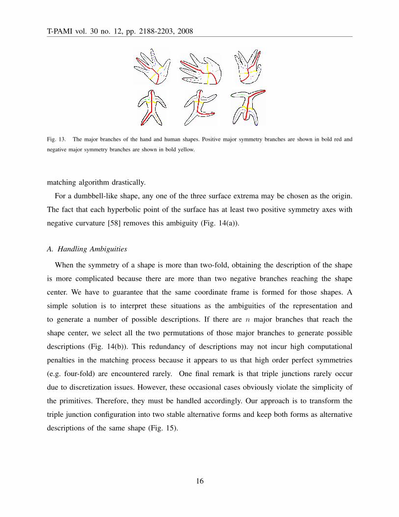
Fig. 13. The major branches of the hand and human shapes. Positive major symmetry branches are shown in bold red and

negative major symmetry branches are shown in bold yellow.

matching algorithm drastically.

For a dumbbell-like shape, any one of the three surface extrema may be chosen as the origin.

The fact that each hyperbolic point of the surface has at least two positive symmetry axes with

negative curvature [58] removes this ambiguity (Fig. 14(a)).

A. Handling Ambiguities

When the symmetry of a shape is more than two-fold, obtaining the description of the shape

is more complicated because there are more than two negative branches reaching the shape

center. We have to guarantee that the same coordinate frame is formed for those shapes. A

simple solution is to interpret these situations as the ambiguities of the representation and

to generate a number of possible descriptions. If there are n major branches that reach the

shape center, we select all the two permutations of those major branches to generate possible

descriptions (Fig. 14(b)). This redundancy of descriptions may not incur high computational

penalties in the matching process because it appears to us that high order perfect symmetries

(e.g. four-fold) are encountered rarely. One final remark is that triple junctions rarely occur

due to discretization issues. However, these occasional cases obviously violate the simplicity of

the primitives. Therefore, they must be handled accordingly. Our approach is to transform the

triple junction configuration into two stable alternative forms and keep both forms as alternative

descriptions of the same shape (Fig. 15).

16

T-PAMI vol. 30 no. 12, pp. 2188-2203, 2008

(a) (b)

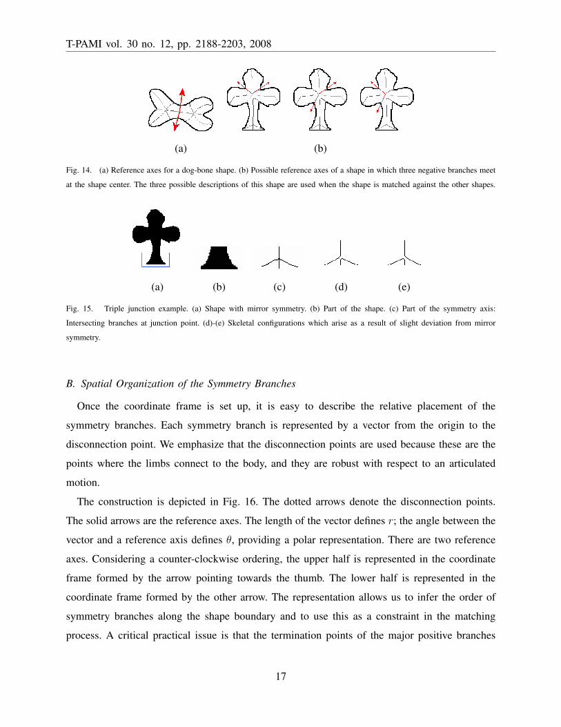
Fig. 14. (a) Reference axes for a dog-bone shape. (b) Possible reference axes of a shape in which three negative branches meet

at the shape center. The three possible descriptions of this shape are used when the shape is matched against the other shapes.

(a) (b) (c) (d) (e)

Fig. 15. Triple junction example. (a) Shape with mirror symmetry. (b) Part of the shape. (c) Part of the symmetry axis:

Intersecting branches at junction point. (d)-(e) Skeletal configurations which arise as a result of slight deviation from mirror

symmetry.

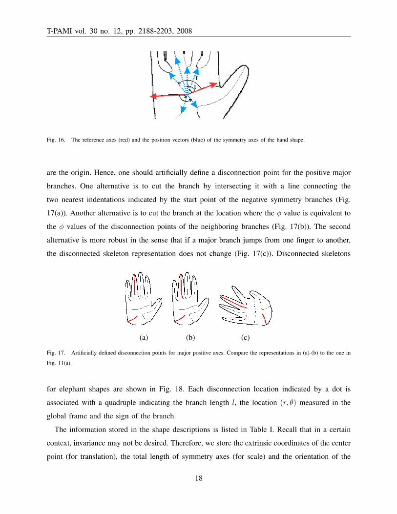
B. Spatial Organization of the Symmetry Branches

Once the coordinate frame is set up, it is easy to describe the relative placement of the

symmetry branches. Each symmetry branch is represented by a vector from the origin to the

disconnection point. We emphasize that the disconnection points are used because these are the

points where the limbs connect to the body, and they are robust with respect to an articulated

motion.

The construction is depicted in Fig. 16. The dotted arrows denote the disconnection points.

The solid arrows are the reference axes. The length of the vector defines r; the angle between the

vector and a reference axis defines θ, providing a polar representation. There are two reference

axes. Considering a counter-clockwise ordering, the upper half is represented in the coordinate

frame formed by the arrow pointing towards the thumb. The lower half is represented in the

coordinate frame formed by the other arrow. The representation allows us to infer the order of

symmetry branches along the shape boundary and to use this as a constraint in the matching

process. A critical practical issue is that the termination points of the major positive branches

17

T-PAMI vol. 30 no. 12, pp. 2188-2203, 2008

Fig. 16. The reference axes (red) and the position vectors (blue) of the symmetry axes of the hand shape.

are the origin. Hence, one should artificially define a disconnection point for the positive major

branches. One alternative is to cut the branch by intersecting it with a line connecting the

two nearest indentations indicated by the start point of the negative symmetry branches (Fig.

17(a)). Another alternative is to cut the branch at the location where the φ value is equivalent to

the φ values of the disconnection points of the neighboring branches (Fig. 17(b)). The second

alternative is more robust in the sense that if a major branch jumps from one finger to another,

the disconnected skeleton representation does not change (Fig. 17(c)). Disconnected skeletons

(a) (b) (c)

Fig. 17. Artificially defined disconnection points for major positive axes. Compare the representations in (a)-(b) to the one in

Fig. 11(a).

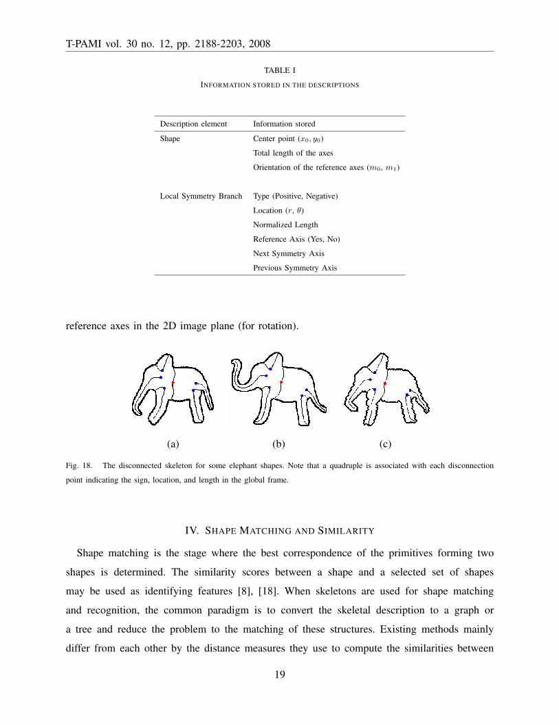
for elephant shapes are shown in Fig. 18. Each disconnection location indicated by a dot is

associated with a quadruple indicating the branch length l, the location (r, θ) measured in the

global frame and the sign of the branch.

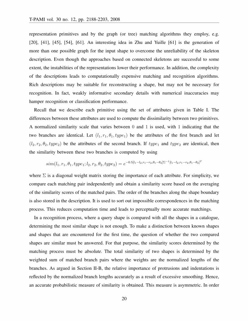
The information stored in the shape descriptions is listed in Table I. Recall that in a certain

context, invariance may not be desired. Therefore, we store the extrinsic coordinates of the center

point (for translation), the total length of symmetry axes (for scale) and the orientation of the

18

T-PAMI vol. 30 no. 12, pp. 2188-2203, 2008

TABLE I

INFORMATION STORED IN THE DESCRIPTIONS

Description element Information stored

Shape Center point (x0, y0)

Total length of the axes

Orientation of the reference axes (m0, m1)

Local Symmetry Branch Type (Positive, Negative)

Location (r, θ)

Normalized Length

Reference Axis (Yes, No)

Next Symmetry Axis

Previous Symmetry Axis

reference axes in the 2D image plane (for rotation).

(a) (b) (c)

Fig. 18. The disconnected skeleton for some elephant shapes. Note that a quadruple is associated with each disconnection

point indicating the sign, location, and length in the global frame.

IV. SHAPE MATCHING AND SIMILARITY

Shape matching is the stage where the best correspondence of the primitives forming two

shapes is determined. The similarity scores between a shape and a selected set of shapes

may be used as identifying features [8], [18]. When skeletons are used for shape matching

and recognition, the common paradigm is to convert the skeletal description to a graph or

a tree and reduce the problem to the matching of these structures. Existing methods mainly

differ from each other by the distance measures they use to compute the similarities between

19

T-PAMI vol. 30 no. 12, pp. 2188-2203, 2008

representation primitives and by the graph (or tree) matching algorithms they employ, e.g.

[20], [41], [45], [54], [61]. An interesting idea in Zhu and Yuille [61] is the generation of

more than one possible graph for the input shape to overcome the unreliability of the skeleton

description. Even though the approaches based on connected skeletons are successful to some

extent, the instabilities of the representations lower their performance. In addition, the complexity

of the descriptions leads to computationally expensive matching and recognition algorithms.

Rich descriptions may be suitable for reconstructing a shape, but may not be necessary for

recognition. In fact, weakly informative secondary details with numerical inaccuracies may

hamper recognition or classification performance.

Recall that we describe each primitive using the set of attributes given in Table I. The

differences between these attributes are used to compute the dissimilarity between two primitives.

A normalized similarity scale that varies between 0 and 1 is used, with 1 indicating that the

two branches are identical. Let (l1, r1, θ1, type1) be the attributes of the first branch and let

(l2, r2, θ2, type2) be the attributes of the second branch. If type1 and type2 are identical, then

the similarity between these two branches is computed by using

sim(l1, r1, θ1, type1; l2, r2, θ2, type2) = e−0.5[l1−l2,r1−r2,θ1−θ2]Σ−1[l1−l2,r1−r2,θ1−θ2]T

where Σ is a diagonal weight matrix storing the importance of each attribute. For simplicity, we

compare each matching pair independently and obtain a similarity score based on the averaging

of the similarity scores of the matched pairs. The order of the branches along the shape boundary

is also stored in the description. It is used to sort out impossible correspondences in the matching

process. This reduces computation time and leads to perceptually more accurate matchings.

In a recognition process, where a query shape is compared with all the shapes in a catalogue,

determining the most similar shape is not enough. To make a distinction between known shapes

and shapes that are encountered for the first time, the question of whether the two compared

shapes are similar must be answered. For that purpose, the similarity scores determined by the

matching process must be absolute. The total similarity of two shapes is determined by the

weighted sum of matched branch pairs where the weights are the normalized lengths of the

branches. As argued in Section II-B, the relative importance of protrusions and indentations is

reflected by the normalized branch lengths accurately as a result of excessive smoothing. Hence,

an accurate probabilistic measure of similarity is obtained. This measure is asymmetric. In order

20

T-PAMI vol. 30 no. 12, pp. 2188-2203, 2008

to retain symmetry, the total similarity value is calculated by using both the weights of the

first shape’s primitives and the second shape’s primitives. The lower one of these two similarity

values is selected.

The matching process is a branch and bound algorithm that searches over all possible match-

ings of two shapes. The worst case complexity of this type of algorithm is high; however,

in practice, the matching process is very fast. The number of shape primitives is small and

additional measures are employed to reduce the number of permutations that need to be tested.

Those matchings that would violate the order constraint are not tested. The generation of a

permutation is stopped when it is determined that the current branch of computation will not be

able to produce a higher similarity value than the current maximum. Finally, the representation

of the shape as two halves in two different coordinate frames makes it possible to reduce the

problem into two half problems providing a drastic decrease in computation time.

A. Examples

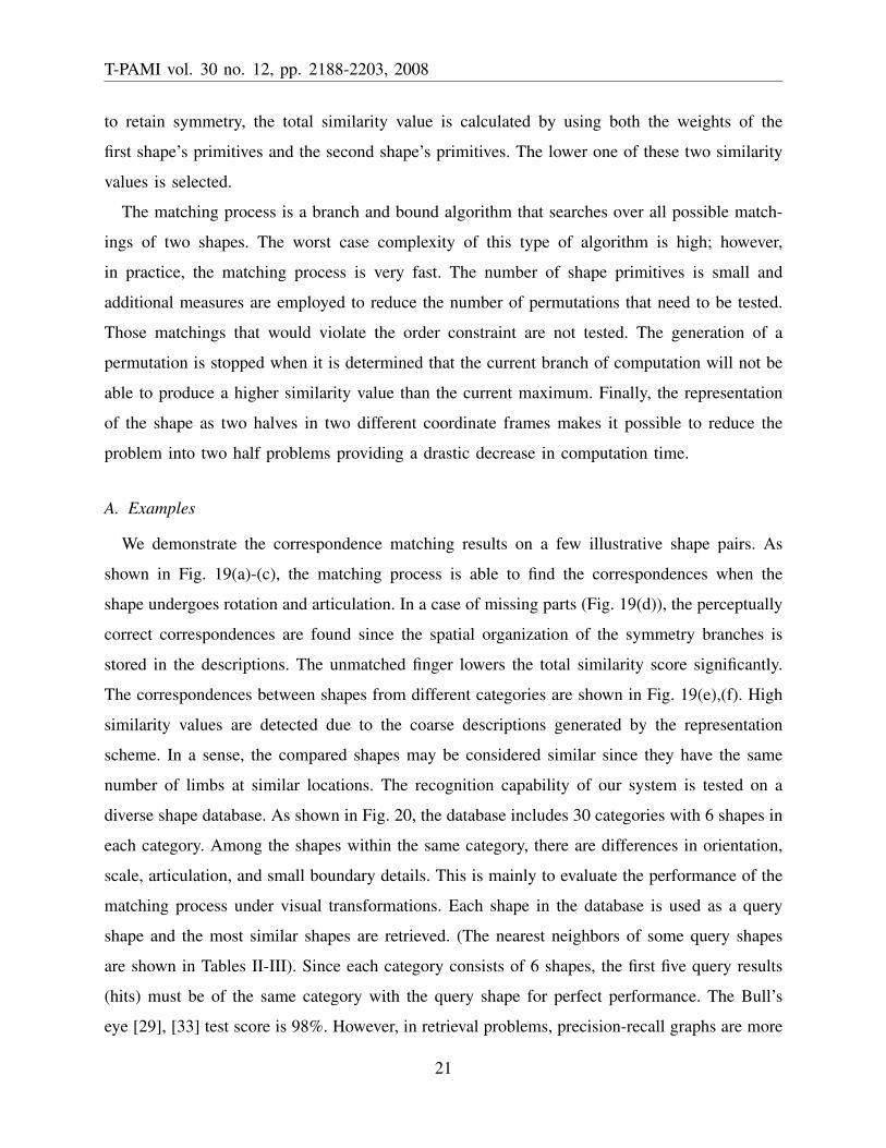
We demonstrate the correspondence matching results on a few illustrative shape pairs. As

shown in Fig. 19(a)-(c), the matching process is able to find the correspondences when the

shape undergoes rotation and articulation. In a case of missing parts (Fig. 19(d)), the perceptually

correct correspondences are found since the spatial organization of the symmetry branches is

stored in the descriptions. The unmatched finger lowers the total similarity score significantly.

The correspondences between shapes from different categories are shown in Fig. 19(e),(f). High

similarity values are detected due to the coarse descriptions generated by the representation

scheme. In a sense, the compared shapes may be considered similar since they have the same

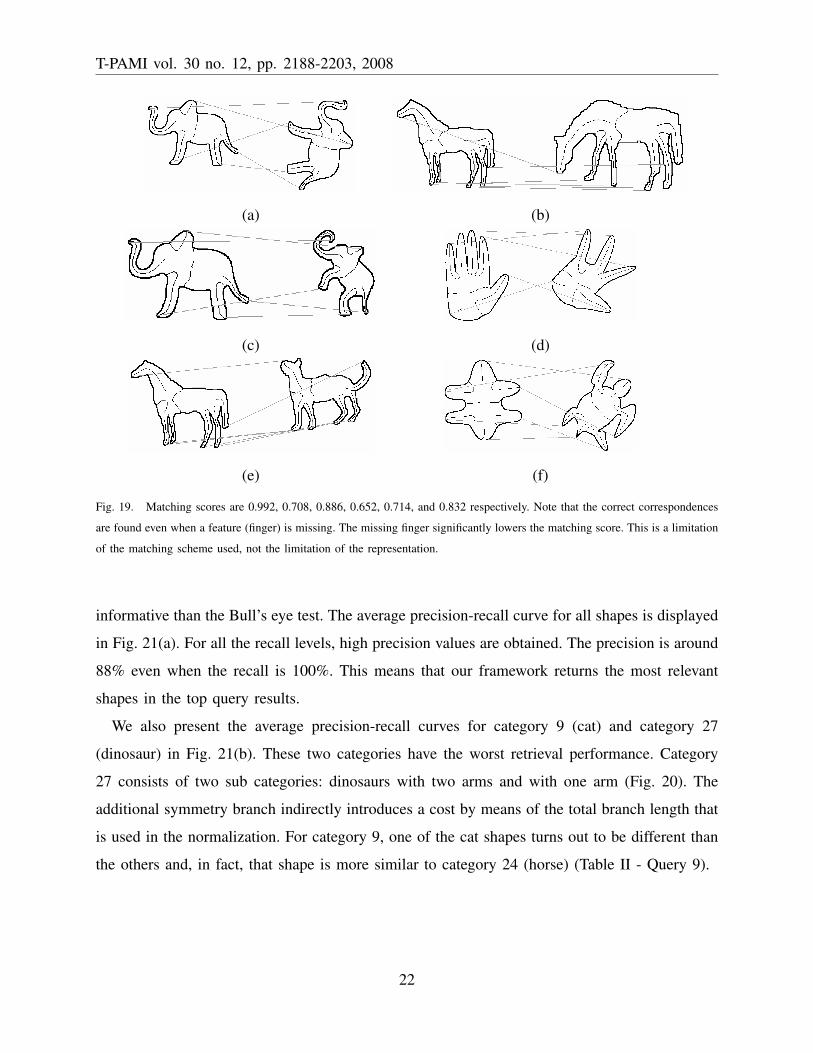
number of limbs at similar locations. The recognition capability of our system is tested on a

diverse shape database. As shown in Fig. 20, the database includes 30 categories with 6 shapes in

each category. Among the shapes within the same category, there are differences in orientation,

scale, articulation, and small boundary details. This is mainly to evaluate the performance of the

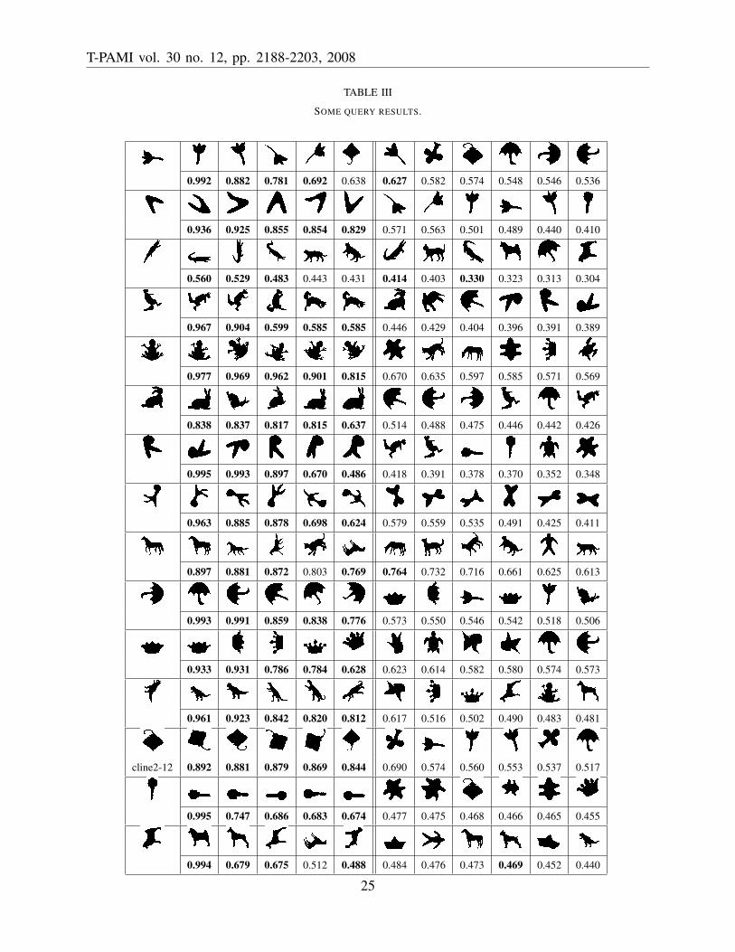
matching process under visual transformations. Each shape in the database is used as a query

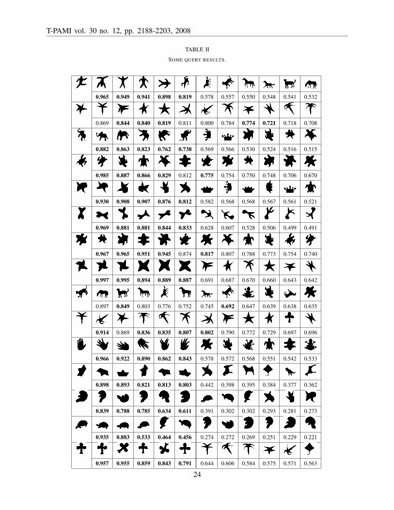
shape and the most similar shapes are retrieved. (The nearest neighbors of some query shapes

are shown in Tables II-III). Since each category consists of 6 shapes, the first five query results

(hits) must be of the same category with the query shape for perfect performance. The Bull’s

eye [29], [33] test score is 98%. However, in retrieval problems, precision-recall graphs are more

21

T-PAMI vol. 30 no. 12, pp. 2188-2203, 2008

(a) (b)

(c) (d)

(e) (f)

Fig. 19. Matching scores are 0.992, 0.708, 0.886, 0.652, 0.714, and 0.832 respectively. Note that the correct correspondences

are found even when a feature (finger) is missing. The missing finger significantly lowers the matching score. This is a limitation

of the matching scheme used, not the limitation of the representation.

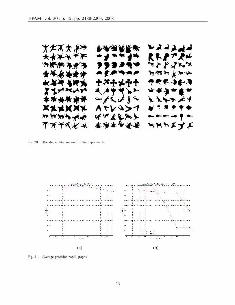
informative than the Bull’s eye test. The average precision-recall curve for all shapes is displayed

in Fig. 21(a). For all the recall levels, high precision values are obtained. The precision is around

88% even when the recall is 100%. This means that our framework returns the most relevant

shapes in the top query results.

We also present the average precision-recall curves for category 9 (cat) and category 27

(dinosaur) in Fig. 21(b). These two categories have the worst retrieval performance. Category

27 consists of two sub categories: dinosaurs with two arms and with one arm (Fig. 20). The

additional symmetry branch indirectly introduces a cost by means of the total branch length that

is used in the normalization. For category 9, one of the cat shapes turns out to be different than

the others and, in fact, that shape is more similar to category 24 (horse) (Table II - Query 9).

22

T-PAMI vol. 30 no. 12, pp. 2188-2203, 2008

Fig. 20. The shape database used in the experiments.

(a) (b)

Fig. 21. Average precision-recall graphs.

23

T-PAMI vol. 30 no. 12, pp. 2188-2203, 2008

TABLE II

SOME QUERY RESULTS.

0.965 0.949 0.941 0.898 0.819 0.578 0.557 0.550 0.548 0.541 0.532

0.869 0.844 0.840 0.819 0.811 0.800 0.784 0.774 0.721 0.718 0.708

0.882 0.863 0.823 0.762 0.738 0.569 0.566 0.530 0.524 0.516 0.515

0.985 0.887 0.866 0.829 0.812 0.775 0.754 0.750 0.748 0.706 0.670

0.930 0.908 0.907 0.876 0.812 0.582 0.568 0.568 0.567 0.561 0.521

0.969 0.881 0.881 0.844 0.833 0.628 0.607 0.528 0.506 0.499 0.491

0.967 0.965 0.951 0.945 0.874 0.817 0.807 0.788 0.773 0.754 0.740

0.997 0.995 0.894 0.889 0.887 0.691 0.687 0.670 0.660 0.643 0.642

0.897 0.849 0.803 0.776 0.752 0.745 0.692 0.647 0.639 0.638 0.635

0.914 0.869 0.836 0.835 0.807 0.802 0.790 0.772 0.729 0.697 0.696

0.966 0.922 0.890 0.862 0.843 0.578 0.572 0.568 0.551 0.542 0.533

0.898 0.893 0.821 0.813 0.803 0.442 0.398 0.395 0.384 0.377 0.362

0.839 0.788 0.785 0.634 0.611 0.391 0.302 0.302 0.293 0.281 0.273

0.935 0.883 0.533 0.464 0.456 0.274 0.272 0.269 0.251 0.229 0.221

0.957 0.955 0.859 0.843 0.791 0.644 0.606 0.584 0.575 0.571 0.563

24

T-PAMI vol. 30 no. 12, pp. 2188-2203, 2008

TABLE III

SOME QUERY RESULTS.

0.992 0.882 0.781 0.692 0.638 0.627 0.582 0.574 0.548 0.546 0.536

0.936 0.925 0.855 0.854 0.829 0.571 0.563 0.501 0.489 0.440 0.410

0.560 0.529 0.483 0.443 0.431 0.414 0.403 0.330 0.323 0.313 0.304

0.967 0.904 0.599 0.585 0.585 0.446 0.429 0.404 0.396 0.391 0.389

0.977 0.969 0.962 0.901 0.815 0.670 0.635 0.597 0.585 0.571 0.569

0.838 0.837 0.817 0.815 0.637 0.514 0.488 0.475 0.446 0.442 0.426

0.995 0.993 0.897 0.670 0.486 0.418 0.391 0.378 0.370 0.352 0.348

0.963 0.885 0.878 0.698 0.624 0.579 0.559 0.535 0.491 0.425 0.411

0.897 0.881 0.872 0.803 0.769 0.764 0.732 0.716 0.661 0.625 0.613

0.993 0.991 0.859 0.838 0.776 0.573 0.550 0.546 0.542 0.518 0.506

0.933 0.931 0.786 0.784 0.628 0.623 0.614 0.582 0.580 0.574 0.573

0.961 0.923 0.842 0.820 0.812 0.617 0.516 0.502 0.490 0.483 0.481

cline2-12 0.892 0.881 0.879 0.869 0.844 0.690 0.574 0.560 0.553 0.537 0.517

0.995 0.747 0.686 0.683 0.674 0.477 0.475 0.468 0.466 0.465 0.455

0.994 0.679 0.675 0.512 0.488 0.484 0.476 0.473 0.469 0.452 0.440

25

T-PAMI vol. 30 no. 12, pp. 2188-2203, 2008

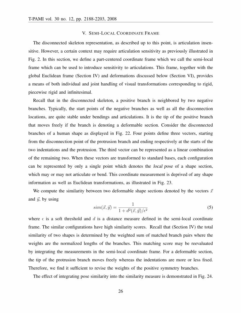
V. SEMI-LOCAL COORDINATE FRAME

The disconnected skeleton representation, as described up to this point, is articulation insen-

sitive. However, a certain context may require articulation sensitivity as previously illustrated in

Fig. 2. In this section, we define a part-centered coordinate frame which we call the semi-local

frame which can be used to introduce sensitivity to articulations. This frame, together with the

global Euclidean frame (Section IV) and deformations discussed below (Section VI), provides

a means of both individual and joint handling of visual transformations corresponding to rigid,

piecewise rigid and infinitesimal.

Recall that in the disconnected skeleton, a positive branch is neighbored by two negative

branches. Typically, the start points of the negative branches as well as all the disconnection

locations, are quite stable under bendings and articulations. It is the tip of the positive branch

that moves freely if the branch is denoting a deformable section. Consider the disconnected

branches of a human shape as displayed in Fig. 22. Four points define three vectors, starting

from the disconnection point of the protrusion branch and ending respectively at the starts of the

two indentations and the protrusion. The third vector can be represented as a linear combination

of the remaining two. When these vectors are transformed to standard bases, each configuration

can be represented by only a single point which denotes the local pose of a shape section,

which may or may not articulate or bend. This coordinate measurement is deprived of any shape

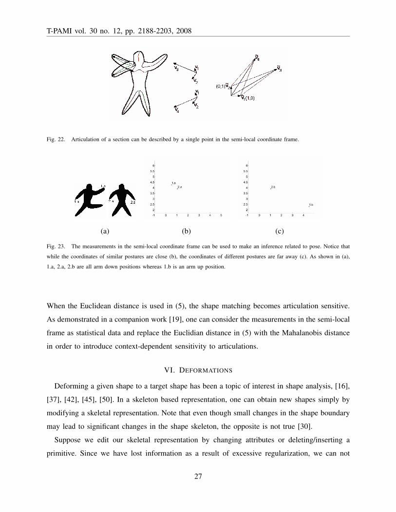
information as well as Euclidean transformations, as illustrated in Fig. 23.

We compute the similarity between two deformable shape sections denoted by the vectors ~x

and ~y, by using

sim(~x, ~y) =1

1 + d2(~x, ~y)/ε2(5)

where ε is a soft threshold and d is a distance measure defined in the semi-local coordinate

frame. The similar configurations have high similarity scores. Recall that (Section IV) the total

similarity of two shapes is determined by the weighted sum of matched branch pairs where the

weights are the normalized lengths of the branches. This matching score may be reevaluated

by integrating the measurements in the semi-local coordinate frame. For a deformable section,

the tip of the protrusion branch moves freely whereas the indentations are more or less fixed.

Therefore, we find it sufficient to revise the weights of the positive symmetry branches.

The effect of integrating pose similarity into the similarity measure is demonstrated in Fig. 24.

26

T-PAMI vol. 30 no. 12, pp. 2188-2203, 2008

Fig. 22. Articulation of a section can be described by a single point in the semi-local coordinate frame.

(a) (b) (c)

Fig. 23. The measurements in the semi-local coordinate frame can be used to make an inference related to pose. Notice that

while the coordinates of similar postures are close (b), the coordinates of different postures are far away (c). As shown in (a),

1.a, 2.a, 2.b are all arm down positions whereas 1.b is an arm up position.

When the Euclidean distance is used in (5), the shape matching becomes articulation sensitive.

As demonstrated in a companion work [19], one can consider the measurements in the semi-local

frame as statistical data and replace the Euclidian distance in (5) with the Mahalanobis distance

in order to introduce context-dependent sensitivity to articulations.

VI. DEFORMATIONS

Deforming a given shape to a target shape has been a topic of interest in shape analysis, [16],

[37], [42], [45], [50]. In a skeleton based representation, one can obtain new shapes simply by

modifying a skeletal representation. Note that even though small changes in the shape boundary

may lead to significant changes in the shape skeleton, the opposite is not true [30].

Suppose we edit our skeletal representation by changing attributes or deleting/inserting a

primitive. Since we have lost information as a result of excessive regularization, we can not

27

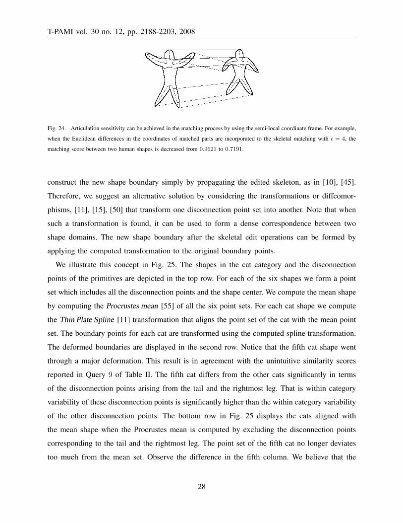
T-PAMI vol. 30 no. 12, pp. 2188-2203, 2008

Fig. 24. Articulation sensitivity can be achieved in the matching process by using the semi-local coordinate frame. For example,

when the Euclidean differences in the coordinates of matched parts are incorporated to the skeletal matching with ε = 4, the

matching score between two human shapes is decreased from 0.9621 to 0.7191.

construct the new shape boundary simply by propagating the edited skeleton, as in [10], [45].

Therefore, we suggest an alternative solution by considering the transformations or diffeomor-

phisms, [11], [15], [50] that transform one disconnection point set into another. Note that when

such a transformation is found, it can be used to form a dense correspondence between two

shape domains. The new shape boundary after the skeletal edit operations can be formed by

applying the computed transformation to the original boundary points.

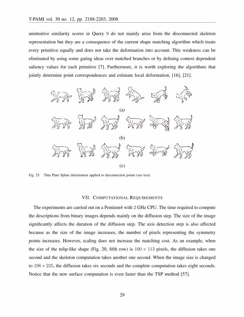
We illustrate this concept in Fig. 25. The shapes in the cat category and the disconnection

points of the primitives are depicted in the top row. For each of the six shapes we form a point

set which includes all the disconnection points and the shape center. We compute the mean shape

by computing the Procrustes mean [55] of all the six point sets. For each cat shape we compute

the Thin Plate Spline [11] transformation that aligns the point set of the cat with the mean point

set. The boundary points for each cat are transformed using the computed spline transformation.

The deformed boundaries are displayed in the second row. Notice that the fifth cat shape went

through a major deformation. This result is in agreement with the unintuitive similarity scores

reported in Query 9 of Table II. The fifth cat differs from the other cats significantly in terms

of the disconnection points arising from the tail and the rightmost leg. That is within category

variability of these disconnection points is significantly higher than the within category variability

of the other disconnection points. The bottom row in Fig. 25 displays the cats aligned with

the mean shape when the Procrustes mean is computed by excluding the disconnection points

corresponding to the tail and the rightmost leg. The point set of the fifth cat no longer deviates

too much from the mean set. Observe the difference in the fifth column. We believe that the

28

T-PAMI vol. 30 no. 12, pp. 2188-2203, 2008

unintuitive similarity scores in Query 9 do not mainly arise from the disconnected skeleton

representation but they are a consequence of the current shape matching algorithm which treats

every primitive equally and does not take the deformation into account. This weakness can be

eliminated by using some gating ideas over matched branches or by defining context dependent

saliency values for each primitive [7]. Furthermore, it is worth exploring the algorithms that

jointly determine point correspondences and estimate local deformation, [16], [21].

(a)

(b)

(c)

Fig. 25. Thin Plate Spline deformation applied to disconnection points (see text).

VII. COMPUTATIONAL REQUIREMENTS

The experiments are carried out on a Pentium4 with 2 GHz CPU. The time required to compute

the descriptions from binary images depends mainly on the diffusion step. The size of the image

significantly affects the duration of the diffusion step. The axis detection step is also affected

because as the size of the image increases, the number of pixels representing the symmetry

points increases. However, scaling does not increase the matching cost. As an example, when

the size of the tulip-like shape (Fig. 20, fifth row) is 100 × 113 pixels, the diffusion takes one

second and the skeleton computation takes another one second. When the image size is changed

to 198× 225, the diffusion takes six seconds and the complete computation takes eight seconds.

Notice that the new surface computation is even faster than the TSP method [57].

29

T-PAMI vol. 30 no. 12, pp. 2188-2203, 2008

Since the representation scheme produces coarse descriptions of shapes, the number of branches

and the number of descriptions are small. Therefore, even the matching of the most complex

shapes in the database takes approximately one second. However, when a shape is compared to all

the shapes in the database, the number of descriptions of the query shape affects the computation

time. For instance, while it takes fifteen seconds to classify a shape with two descriptions, it takes

twenty-five seconds to classify a shape with six descriptions. Because of the fixed complexity

of retrieving shapes from storage, the change in computation time is not as high as expected.

VIII. SUMMARY AND DISCUSSION

We have presented an unconventional approach to shape representation and recognition by

using skeletons. Unlike common skeletal representations, our branches are disconnected as a

result of excessive regularization. Hence, the representation is a point set representation. A key

difference in our framework from the conventional approach is the construction of separate

mechanisms to handle visual transformations. The main focus of this paper is the global frame

that is constructed to handle scale, rotation and translation. This frame, alone, is sufficient for

articulation insensitive similarity measurement.

We have demonstrated the potential of the representation on shape matching and similarity

computation. On a diverse shape database of 180 shapes with 30 categories, even for a 100%

recall rate, the precision is over 88%. The Bull’s eye [29], [33] test score is 98%. Even though the

shapes are represented at attainable coarseness, the matching results are comparable to skeletal

representations with complete detail. We offer the following explanation. Very large numbers of

explanatory features are harmful for recognition and categorization tasks. Secondary details which

are weakly informative contain errors due to numerics and lower the recognition performance.

Hence, relying on dominant features that can be extracted with high numerical accuracy alleviates

the problem.

The presented method is easy to implement and fast to compute. The disconnected nature of our

skeletal representation not only introduces robustness, but also makes the necessary constructions

almost trivial.

An important weakness of the method is that it is limited to shapes with closed boundaries.

Even though we can compute symmetry axes for the shapes with holes, construction of the

complete representation along with the coordinate frame constructions becomes tricky. A major

30

T-PAMI vol. 30 no. 12, pp. 2188-2203, 2008

limitation comes from the fact that shapes with holes are not easily shrunk to single centers. A

simple surface minimum indicating the center is replaced with a sequence of parabolic points

whose centroid is typically outside the shape. Currently, we are working on extending the

construction of disconnected skeleton to shapes with holes.

REFERENCES

[1] L. Ambrosio and V. Tortorelli. On the approximation of functionals depending on jumps by elliptic functionals via

Γ-convergence. Commun. Pure Appl. Math., 43(8):999–1036, 1990.

[2] C. Aslan. Disconnected skeletons for shape recognition. Master’s thesis, Department of Computer Engineering, Middle

East Technical University, May 2005.

[3] C. Aslan, A. Erdem, E. Erdem, and S. Tari. Supplemental material. http://computer.org/tpami/archives.htm.

[4] C. Aslan and S. Tari. An axis-based representation for recognition. In ICCV, pages 1339–1346, 2005.

[5] J. August, K. Siddiqi, and S. W. Zucker. Ligature instabilities in the perceptual organization of shape. Comput. Vis. Image

Underst., 76(3):231–243, 1999.

[6] X. Bai, L. J. Latecki, and W.-Y. Liu. Skeleton pruning by contour partitioning with discrete curve evolution. IEEE Trans.

Pattern Anal. Mach. Intell., 29(3):449–462, 2007.

[7] E. Baseski. Context–sensitive matching of two shapes. Master’s thesis, Department of Computer Engineering, Middle East

Technical University, July 2006.

[8] R. Basri. Recognition by prototypes. In CVPR, pages 161–167, 1993.

[9] S. Belongie, J. Malik, and J. Puzicha. Shape matching and object recognition using shape contexts. IEEE Trans. Pattern

Anal. Mach. Intell., 24(4):509–522, 2002.

[10] H. Blum. Biological shape and visual science. Journal of Theoretical Biology, 38:205–287, 1973.

[11] F. L. Bookstein. Morphometric Tools for Landmark Data–Geometry and Biology. Cambridge Univ. Press, 1991.

[12] M. Brady and H. Asada. Smoothed local symmetries and their implementation. The International Journal of Robotics

Research, 3(3):36–61, 1984.

[13] J.W. Bruce, P.J. Giblin, and C.G. Gibson. Symmetry sets. Proc. R. Soc. Edinb. Sect. A-Math, 101:163–186, 1985.

[14] M. C. Burl and P. Perona. Recognition of planar object classes. In CVPR, pages 223–230, 1996.

[15] V. Camion and L. Younes. Geodesic interpolating splines. In EMMCVPR, pages 513–527, 2001.

[16] H. Chui and A. Rangarajan. A new point matching algorithm for non-rigid registration. CVIU, 89(2-3):114–141, 2003.

[17] A. R. Dill, M. D. Levine, and P. B. Noble. Multiple resolution skeletons. IEEE Trans. Pattern Anal. Mach. Intell.,

9(4):495–504, 1987.

[18] S. Edelman. Representation is representation of similarities. Behavioral and Brain Sciences, 21(4):449–498, 1998.

[19] A. Erdem, E. Erdem, and S. Tari. Articulation prior in an axial representation. In International Workshop on the

Representation and Use of Prior Knowledge in Vision (WRUPKV) held in association with ECCV06, pages 1–14, 2006.

[20] D. Geiger, T. L. Liu, and R. V. Kohn. Representation and self-similarity of shapes. IEEE Trans. Pattern Anal. Mach.

Intell., 25(1):86–99, 2003.

[21] J. Glaunes, A. Trouve, and L. Younes. Diffeomorphic matching of distributions: A new approach for unlabelled point-sets

and sub-manifolds matching. In CVPR, pages 712–718, 2004.

31

T-PAMI vol. 30 no. 12, pp. 2188-2203, 2008

[22] L. Gorelick, M. Galun, E. Sharon, R. Basri, and A. Brandt. Shape representation and classification using the poisson

equation. IEEE Trans. Pattern Anal. Mach. Intell., 28(12):1991–2005, December 2006.

[23] J. Goutsias and D. Schonfeld. Morphological representation of discrete and binary images. IEEE Trans. Pattern Anal.

Mach. Intell., 39(6):1369–1379, 1991.

[24] D. G. Kendall, D. Barden, T. K. Carne, and H. Le. Shape and Shape Theory. John Wiley and Sons, 1999.

[25] B. B. Kimia, A. R. Tannenbaum, and S. W. Zucker. Shapes, shocks, and deformations I: The components of two-dimensional

shape and the reaction-diffusion space. Int. J. Comput. Vision, 15(3):189–224, 1995.

[26] R. Kresch. Morphological Image Representation for Coding Applications. PhD thesis, Technion Israel Inst. Technol.,

1995.

[27] R. Kresch and D. Malah. Morphological reduction of skeleton redundancy. Signal Processing, 38:143–151, 1994.

[28] C. Lantuejoul. La squelettisation et son application aux mesures topologiques des mosaques polycristallines. PhD thesis,

Ecole des Mines de Paris, 1978.

[29] L. J. Latecki and R. Lakamper. Shape similarity measure based on correspondence of visual parts. IEEE Trans. Pattern

Anal. Mach. Intell., 22(10):1185–1190, 2000.

[30] K. Leonard. Classification of 2D shapes via efficiency measures. 2006. Unpublished work.

[31] G. Levi and U. Montanari. A grey-weighted skeleton. Information and Control, 17(1):62–91, 1970.

[32] M. Leyton. A process-grammar for shape. Artificial Intelligence, 34(2):213–247, 1988.

[33] H. Ling and D. W. Jacobs. Using the inner-distance for classification of articulated shapes. In CVPR, pages 719–726,

2005.

[34] P. Maragos. Pattern spectrum and multiscale shape representation. IEEE Trans. Pattern Anal. Mach. Intell., 11(7):701–716,

1989.

[35] P. Maragos and R. W. Schafer. Morphological skeleton representation and coding of binary images. IEEE Trans. on

Acoustics, Speech, and Signal Processing, 34(5):1228–1244, 1986.

[36] G. Matheron. Random Sets and Integral Geometry. Wiley, 1975.

[37] W. Mio, A. Srivastava, and S. Joshi. On shape of plane elastic curves. Int. J. Comput. Vision, 73(3):307–324, 2007.

[38] D. Mumford and J. Shah. Optimal approximations by piecewise smooth functions and associated variational problems.

Commun. Pure Appl. Math., 42(5):577–685, 1989.

[39] R. Ogniewicz and O. Kubler. Hierarchic voronoi skeletons. Pattern Recognition, 28(3):343–359, 1995.

[40] O. C. Ozcanli, A. Tamrakar, B. B. Kimia, and J. L. Mundy. Augmenting shape with appearance in vehicle category

recognition. In CVPR, pages 935–942, 2006.

[41] M. Pelillo, K. Siddiqi, and S. W. Zucker. Matching hierarchical structures using association graphs. IEEE Trans. Pattern

Anal. Mach. Intell., 21(11):1105–1120, 1999.

[42] A. Peter and A. Rangarajan. Shape matching using the Fisher-Rao Riemannian metric: Unifying shape representation and

deformation. In 2006 IEEE International Symposium on Biomedical Imaging: From Nano to Macro, pages 1164–1167,

2006.

[43] S. M. Pizer, W. R. Oliver, and S.H. Bloomberg. Hierarchical shape description via the multiresolution symmetric axis

transform. IEEE Trans. Pattern Anal. Mach. Intell., 9(4):505–511, 1987.

[44] S. M. Pizer, K. Siddiqi, G. Szekely, J. N. Damon, and S. W. Zucker. Multiscale medial loci and their properties. Int. J.

Comput. Vision, 55(2-3):155–179, 2003.

32

T-PAMI vol. 30 no. 12, pp. 2188-2203, 2008

[45] T. B. Sebastian, P. N. Klein, and B. B. Kimia. Recognition of shapes by editing their shock graphs. IEEE Trans. Pattern

Anal. Mach. Intell., 26(5):550–571, 2004.

[46] J. Serra. Image Analysis and Mathematical Morphology. London Academic Press, Inc., Orlando, FL, USA, 1982.

[47] J. Shah. Segmentation by nonlinear diffusion II. In CVPR, pages 644–647, 1992.

[48] J. Shah. A common framework for curve evolution, segmentation and anisotropic diffusion. In CVPR, pages 136–142,

1996.

[49] J. Shah. Grayscale skeletons and segmentation of shapes. CVIU, 99(1):96–109, 2005.

[50] J. Shah. An H2 type Riemannian metric on the space of planar curves. In Workshop on the Mathematical Foundations of

Computational Anatomy (in conjunction with MICCAI’06), pages 40–46, 2006.

[51] D. Shaked and A. M. Bruckstein. Pruning medial axes. CVIU, 69(2):156–169, 1998.

[52] K. Siddiqi, S. Bouix, A. Tannenbaum, and S. W. Zucker. Hamilton-Jacobi skeletons. Int. J. Comput. Vision, 48(3):215–231,

2002.

[53] K. Siddiqi and B. B. Kimia. A shock grammar for recognition. In CVPR, pages 507–513, 1996.

[54] K. Siddiqi, A. Shokoufandeh, S. J. Dickinson, and S. W. Zucker. Shock graphs and shape matching. Int. J. Comput.

Vision, 35(1):13–32, 1999.

[55] C. Small. The Statistical Theory of Shape. Springer, 1996.

[56] S. Tari and J. Shah. Local symmetries of shapes in arbitrary dimension. In ICCV, pages 1123–1128, 1998.

[57] S. Tari, J. Shah, and H. Pien. A computationally efficient shape analysis via level sets. In MMBIA ’96: Proceedings of

the 1996 Workshop on Mathematical Methods in Biomedical Image Analysis (MMBIA ’96), pages 234–243, 1996.

[58] S. Tari, J. Shah, and H. Pien. Extraction of shape skeletons from grayscale images. CVIU, 66(2):133–146, 1997.

[59] M. van Eede, D. Macrini, A. Telea, C. Sminchisescu, and S. Dickinson. Canonical skeletons for shape matching. In ICPR,

volume 2, pages 64–69, 2006.

[60] S. C. Zhu. Stochastic jump-diffusion process for computing medial axes in markov random fields. IEEE Trans. Pattern

Anal. Mach. Intell., 21(11):1158–1169, 1999.

[61] S. C. Zhu and A. L. Yuille. FORMS: A flexible object recognition and modeling system. Int. J. Comput. Vision, 20(3):187–

212, 1996.

ACKNOWLEDGMENTS

We thank J. Shah, D. Sezer, J. Scheideman, K. Hulten, and anonymous reviewers for providing

feedback. Preliminary version by C. Aslan and S. Tari has appeared in [4].

33