Discrete adjoint method in elsA (part I): method/theory.

J. Peter

7th ONERA-DLR Aerospace SymposiumTOULOUSE, FRANCE 4-6 octobre 2006

TP 2006-163 TP 2006-163

Discrete adjoint method in elsA (part I):

method/theory.

Méthode adjointe discrète dans elsA

(partie I) : méthode, théorie.

par

J. Peter

Résumé Traduit : Cet article décrit les activités récentes de l'ONERA dans le domaine de l'optimisation de formes aérodyamiques parméthode de gradient. La méthode de l'équation linéarisée discrète et la méthode de l'équation adjointe discrète ont étéconsidérées pour le calcul de la dérivée d'une fonction aérodynamique par rapport aux paramètres de forme. Laméthode numérique de calcul de l'écoulement (on résout les équations RANS) et de calcul des gradients sontbrièvement décrites. On présente la linéarisation du modèle k-omega de Wiilcox, pour améliorer la précision desméthodes de calcul de gradient standard avec "figeage" du coefficient de viscosité. On décrit aussi deux techniquesd'amélioration de la robustesse de la résolution itérative de l'équation adjointe discrète. Enfin, on présente l'extension dece travail aux configurations de turbomachines.

NB : Ce Tiré à part fait référence au Document d'Accompagnement de Publication DSNA0639

DISCRETE ADJOINT METHOD IN elsA (PART I) :METHOD/THEORY

J. Peter (Jacques.Peter@onera.fr)ONERA BP 72 - 29 av. de la Division Leclerc 92322 CHATILLON CEDEX

Abstract

This paper describes the recent activities developed at ONERA in the field of aerodynamicshape optimization using gradient based methods. Both discrete direct differentiation methodand discrete adjoint method have been considered for the computation of the derivatives of afunction with respect to the design parameters. The numerical methods for flow computations(solving RANS equations) and for gradient computations are briefly described. The linearizationof Wilcox (

�����) model for improving accuracy of standart gradient computation method - with

“ frozen ” turbulent viscosity - is presented. Also described are two techniques for robustnessenhancement of iterative resolution of discrete adjoint equation. Finally, the extension of thisframework to turbomachinery is briefly presented.

Fluid Dynamics / Shape optimization / Gradient Computation / Adjoint Method / Direct Dif-ferentiation Method.

1 INTRODUCTIONThe aim of aerodynamic design optimization is the minimization of an objective function subjectto a set of constraints. A classical example and a main application in aerodynamic design is thedrag-reduction of an aircraft under constraints relating to the lift, the geometry or the momentums.Optimization methods using computational fluid dynamics became popular tools during the lastdecade, reducing the costs associated with wind-tunnel tests. Among the methods currently used aregradient-based optimizers in which the gradients of the functions with respect to (w.r.t.) the designvariables are used to update the design variables, in order to systematically reduce the cost functionto arrive at a local minimum. An important step in this process is the determination of these gradientswhich are also referred to as sensitivity derivatives. As objective and constraints functions are non-linear functions of the conservative variables vector and the geometric variables vector which areconnected by the flow equations, the computation of derivatives is not easy and several techniqueshave been investigated for evaluating these sensitivities.The (discrete) direct differentiation methods and the (continuous or discrete) adjoint variable meth-ods have been proposed around 1990

��� �� . They only involve linear system resolution, in contrast

with the old and expensive finite difference method which requires flow computation for shifedmeshes. Both discrete direct differentiation method and discrete adjoint vector method have beendeveloped at ONERA. The basic numerical method is briefly described in the first part. The secondpart presents linearization of Wilcox ( � ��� ) model for improving accuracy of gradient computa-tions. The third part describes two techniques for enhancing the robustness of the iterative resolutionof the adjoint equation.

2 NUMERICAL METHODSThe basic choices were already described � � � . They are summarized in this section.

2.1 Equations of the direct and adjoint variable methodsThe discrete residual of the steady state flow equations can be written as������������� �

(1)

1

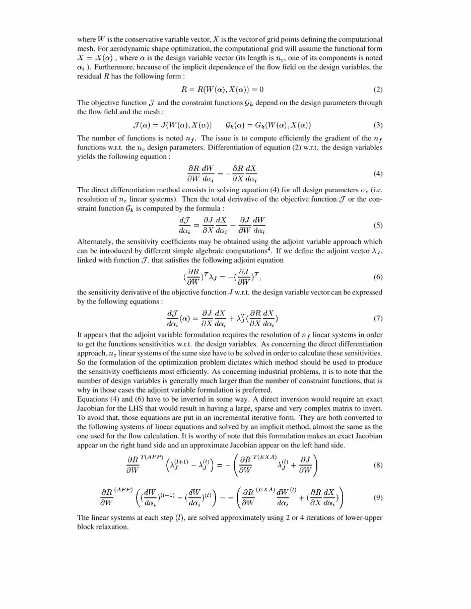
where ! is the conservative variable vector, " is the vector of grid points defining the computationalmesh. For aerodynamic shape optimization, the computational grid will assume the functional form"$#%"'&)(+* , where ( is the design variable vector (its length is ,+- , one of its components is noted(+. ). Furthermore, because of the implicit dependence of the flow field on the design variables, theresidual / has the following form :/0# /�&)!1&)(+*2�"'&)(+*3*4#65 (2)

The objective function 7 and the constraint functions 8:9 depend on the design parameters throughthe flow field and the mesh :7;&<(=*4#%>�&�!1&<(=*�2�"?&<(=*�* 8 9 &<(=*4# @ 9 &)!1&)(+*2�"'&)(+*3* (3)

The number of functions is noted ,+A . The issue is to compute efficiently the gradient of the ,+Afunctions w.r.t. the ,B- design parameters. Differentiation of equation (2) w.r.t. the design variablesyields the following equation : C /C ! D !D (+. #FE C /C " D "D (B. (4)

The direct differentiation method consists in solving equation (4) for all design parameters (�. (i.e.resolution of ,B- linear systems). Then the total derivative of the objective function 7 or the con-straint function 8G9 is computed by the formula :D 7D (+. # C >C " D "D (+. H C >C ! D !D (B. (5)

Alternately, the sensitivity coefficients may be obtained using the adjoint variable approach whichcan be introduced by different simple algebraic computations I . If we define the adjoint vector JGK ,linked with function 7 , that satisfies the following adjoint equation& C /C ! *�LBJ K #FEM& C >C ! *�L42 (6)

the sensitivity derivative of the objective function > w.r.t. the design variable vector can be expressedby the following equations : D 7D (+. &<(=*4# C >C " D "D (B. H J L K & C /C " D "D (+. * (7)

It appears that the adjoint variable formulation requires the resolution of ,=A linear systems in orderto get the functions sensitivities w.r.t. the design variables. As concerning the direct differentiationapproach, , - linear systems of the same size have to be solved in order to calculate these sensitivities.So the formulation of the optimization problem dictates which method should be used to producethe sensitivity coefficients most efficiently. As concerning industrial problems, it is to note that thenumber of design variables is generally much larger than the number of constraint functions, that iswhy in those cases the adjoint variable formulation is preferred.Equations (4) and (6) have to be inverted in some way. A direct inversion would require an exactJacobian for the LHS that would result in having a large, sparse and very complex matrix to invert.To avoid that, those equations are put in an incremental iterative form. They are both converted tothe following systems of linear equations and solved by an implicit method, almost the same as theone used for the flow calculation. It is worthy of note that this formulation makes an exact Jacobianappear on the right hand side and an approximate Jacobian appear on the left hand side.C /C ! LONQPSR:ROT�U J NWVQXBYZTK E[J NQVWTK�\ #]E_^ C /C ! LONQ`BabPST J NWVQTK H C >C !dc (8)C /C ! NQPSR:ROTbe & D !D (B. *fNQVWXBY�TBEg& D !D (+. *fNQVWTih #FE ^ C /C ! NQ`:abPST D !D (B. NWVWT H & C /C " D "D (+. * c (9)

The linear systems at each step &)j)* , are solved approximately using 2 or 4 iterations of lower-upperblock relaxation.

2

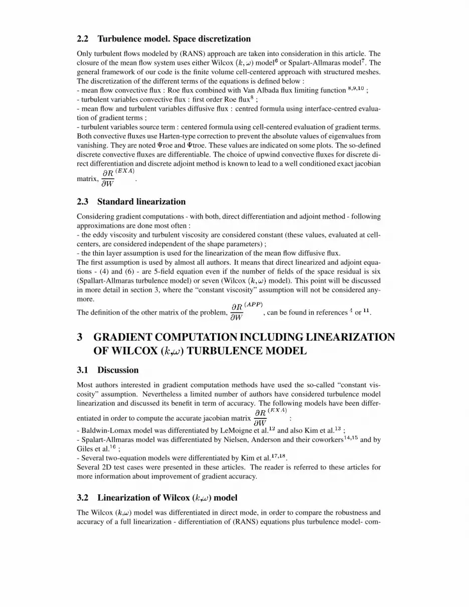
2.2 Turbulence model. Space discretizationOnly turbulent flows modeled by (RANS) approach are taken into consideration in this article. Theclosure of the mean flow system uses either Wilcox k�lGmZn ) model o or Spalart-Allmaras model p . Thegeneral framework of our code is the finite volume cell-centered approach with structured meshes.The discretization of the different terms of the equations is defined below :- mean flow convective flux : Roe flux combined with Van Albada flux limiting function qsr tr uZv ;- turbulent variables convective flux : first order Roe flux q ;- mean flow and turbulent variables diffusive flux : centred formula using interface-centred evalua-tion of gradient terms ;- turbulent variables source term : centered formula using cell-centered evaluation of gradient terms.Both convective fluxes use Harten-type correction to prevent the absolute values of eigenvalues fromvanishing. They are noted w roe and w troe. These values are indicated on some plots. The so-defineddiscrete convective fluxes are differentiable. The choice of upwind convective fluxes for discrete di-rect differentiation and discrete adjoint method is known to lead to a well conditioned exact jacobian

matrix, xzyxS{}|Q~:�b�S� .2.3 Standard linearizationConsidering gradient computations - with both, direct differentiation and adjoint method - followingapproximations are done most often :- the eddy viscosity and turbulent viscosity are considered constant (these values, evaluated at cell-centers, are considered independent of the shape parameters) ;- the thin layer assumption is used for the linearization of the mean flow diffusive flux.The first assumption is used by almost all authors. It means that direct linearized and adjoint equa-tions - (4) and (6) - are 5-field equation even if the number of fields of the space residual is six(Spallart-Allmaras turbulence model) or seven (Wilcox k)lSmZn�� model). This point will be discussedin more detail in section 3, where the “constant viscosity” assumption will not be considered any-more.

The definition of the other matrix of the problem, xGyxS{}|Q�S�O�:� , can be found in references � or u�u .3 GRADIENT COMPUTATION INCLUDING LINEARIZATION

OF WILCOX ( � , � ) TURBULENCE MODEL

3.1 DiscussionMost authors interested in gradient computation methods have used the so-called “constant vis-cosity” assumption. Nevertheless a limited number of authors have considered turbulence modellinearization and discussed its benefit in term of accuracy. The following models have been differ-

entiated in order to compute the accurate jacobian matrix xGyxS{}|Q~B�b�S� :- Baldwin-Lomax model was differentiated by LeMoigne et al. u�� and also Kim et al. u�� ;- Spalart-Allmaras model was differentiated by Nielsen, Anderson and their coworkers uZ�sr u�� and byGiles et al. uZo ;- Several two-equation models were differentiated by Kim et al. u�pr u�q .Several 2D test cases were presented in these articles. The reader is referred to these articles formore information about improvement of gradient accuracy.

3.2 Linearization of Wilcox ( � , � ) modelThe Wilcox ( l , n ) model was differentiated in direct mode, in order to compare the robustness andaccuracy of a full linearization - differentiation of (RANS) equations plus turbulence model- com-

3

pared to those of the standard linearization - differentiation of (RANS) equations, constant turbulentviscosity. The different terms of the turbulent variable equations were differentiated in the followingway :- convective flux : no approximation ;- diffusive flux : no approximation ;- source term : using a decomposition of the term along mesh-lines.The terms of implicit stage matrix - ������?���S�O�O� - for the coupled problem can be found in �3� .3.3 ValidationThe test case is a transonic flow around the NACA64A212 airfoil. The upstream flow characteristicsare : �'����� �¢¡¤£¦¥}§©¨���ª«� £��¦¬�¥®­¤�¯��ª«� °²± . The flow is transonic. The mesh size is 257*65.There is only one design parameter, whose positive variation causes the thickening of the rear partof the suction side. The flow sensitivity is studied and also the derivatives of three aerodynamicfunctions w.r.t. the shape parameter : the lift (noted ³©´ ), the far-field drag and the near-field drag(noted ³©µ ¶S¶ and ³©µ¸·:¶ ) as defined in ��¹ . Finite-differences for flow- and functions-sensitivitiesare calculated from flow calculations on shifted-meshes with a centered formula (actually, flow fieldsº1»�¼ � � £�½ and

º1»¿¾ � � £�½ were computed using corresponding meshes, À »Z¼ � �«£�½ and À »�¾ � �«£Á½ ).Several variable sensitivity plots in the cells adjacent to the wall are presented in figures 1 to 3. Thesensitivity of ( ²à ) near the trailing edge is presented in figures 4 -finite difference- and 5 -solutionof linearized equation. From those figures and the corresponding plots for the other variables, itappears that the flow sensitities of all variables (mean flow and turbulent variables) is quite correctlycomputed using the full linearization approach, the accuracy being higher for the mean flow vari-ables. When comparing mean flow sensitivities obtained by standard and full linearization approach,it appears that the accuracy is improved by full linearization. It can be seen in particular in figures1 and 2 : the standard linearization leads to an significant error at the upper-side, near the shock,whereas the full linearization leads to an accurate solution at this location.The function sensitivities are presented in table 1. The accuracy improvement due to full lineariza-tion is confirmed by these results. Indeed, the full linearization derivatives are closer to the finite dif-ference values, than the standard linearization derivatives for all three functions. The gap beetweenfull linearization values and finite difference reference value for ³©µ ¶S¶ and ³©µ¸·:¶ is difficult toexplain. It may be caused by the lack of convergence in flow computations or by the remaining

approximations in the “exact” jacobian Ä §Ä º �QÅBÆÇ�S�Fonction finite diff. “frozen ÈOÉ ” lin. full (RANS)+( Ê ¼ à ) lin.³©´ 3.82 10-1 3.99 10-1 3.83 10-1³©µ ¶S¶ 2.34 10-3 2.85 10-3 2.68 10-3³©µ¸·:¶ 3.19 10-3 3.87 10-3 3.67 10-3

Table 1: NACA64A212. Comparison of aerodynamic function-sensitivities.

4 ROBUSTNESS ENHANCEMENT OF ADJOINT GRADIENTCOMPUTATION METHOD

4.1 Definition of robustness enhancement techniquesThe iterative process defined by equations (8) and (9) appeared to diverge for some complex config-urations. This lack of convergence was observed even with the standard “frozen È+É approximation”which is used for all 3D complex configurations. Hence, different techniques were considered inorder to enhance the robustness of the resolution of adjoint equation (which is used for the complex

4

applications). Two of them appeared to be efficient. They will be noted (FO) and (AD) :- (FO) - switch to first order linearization of mean flow convective flux for some domains. Even ifthe explicit residual Ë is computed from second order Roe flux plus MUSCL approach (Van Albada

limiting function), the jacobian Ì ËÌSÍ}ÎQÏ:ÐbÑSÒ may include for some domains the linearization of thebasic first-order Roe flux ;

- (AD) - add a dissipative term in Ì ËÌSÍ}ÎQÏBÐÇÑSÒ . Even if the residual Ë includes no artificial dissipa-

tion, an artificial dissipation term may be included in Ì ËÌSÍ ÎQÏ:ÐbÑSÒ . It is not defined by linearization

of a classical artificial dissipation term -as defined in Ó3Ô for example-, but by directly applying thiskind of formula to the adjoint vector.

4.2 Application to ONERA M6 wingThe test case for this study is the ONERA M6 Wing. The upstream flow characteristics are Õ×ÖFØ Ù¦ÚË©ÛMÖ�Ü¦Ø Ú²ÝÞÜàß²á . Four angles of attack are considered â ãäÖ%ß²å�æsÜ�å�æ�ç¦åèæ3éêå . The 10-block mesh con-tains 620042 points. The design parameter is the angle of rotation around the axis ( ë�Ö�ß , ìíÖ_ß ).The function to derivate is the lift î©ï . Without the techniques (FO) and (AD), the iterative processdefined by equation (8) fails to converge, after a reduction of two to three orders of magnitude ofthe right hand side of the equation. Different numerical experiments were carried out with (FO) and(AD) techniques.- Applying (AD) technique improves the best convergence level (to more than three orders of mag-nitude), but all four adjoint gradient computations exhibit finally a divergent behaviour. The mostappropriate coefficients for the artificial dissipation have low values - about ð Ó = .004, ð¦ñ =0.00025-,much lower than those used for analysis computation with a centered scheme.- Applying (FO) technique to two blocks located downstream the wing - blocks 9 and 10, see figure(6)-, which are not adjacent to the wall, enables the convergence of adjoint gradient computation fortwo of the four computations - â�Ö ßêå , â¸ÖFÜ Ô . The convergence of the two other computations canbe obtained with a blend of (FO) and (AD) techniques. The values of the corresponding artificialdissipation coefficients and the convergence plots are presented in figure (7).- Applying (FO) technique to two blocks located downstream the wing - blocks 1, 9 and 10, seefigure (6)- which are not adjacent to the wall, enables the convergence of all four adjoint gradientcomputation. The corresponding convergence plots are presented in figure (8).

5 EXTENSION TO TURBOMACHINERY

5.1 TheoryThe numerical methods presented beforehand are currently being extended to turbomachinery flows.This work consists first in differentiating the fluxes and the boundary term, that are used specificallyin turbomachinery flow computations :- the inertial term of the “relative frame/relative velocity” formulation, which is considered for thesimulation of the flow around rotating bladings ;- the subsonic inlet condition ;- the various subsonic exit conditions (fixed static pressure, radial equilibrium, fixed mass flow...).Second, the derivatives of the functions of interest w.r.t the flow field and the mesh are calculed. Thistask is carried out by the DAAP/H2T team.

5.2 ApplicationSeveral nozzle and blade configurations have already been considered. The geometric deformationfor blades is a rotation in (yz) planes (normal to the machine-axis). The angle of rotation increases

5

linearly from hub to casing and the design parameter is the maximum angle of rotation (applied atthe casing). We briefly discuss the accuracy of gradient for two geometries :- the rotating ventilators of ONERA S1MA wind-tunnel ò�ó . Discrete Euler equations are solved. Themass flow is ôöõö÷�ø«ù�÷àø²úûêü ýèþ , the rotational speed is ÿ õ � ÷ ������� , the shaft power is 44 Mwand the resulting Mach number at the tip is 0.6. The functions to be derived are the integrals ofconservatives variables and static temperature in the outlet section. ;- the static blade of generic configuration called RED3D. The mass flow is ôFõF÷����¦ûêü ýèþ , the rationof static pressure (outlet to inlet) is ���� ��� õ�ù ��� � , and the deviation is about ����� . The physical modelare the (RANS) equations and Wilcox (k-l) turbulence model. The function to be differentiated w.r.t.the design parameters are the same as in the first test case.The derivatives and their deviation to finite difference references are presented in the next two tables.

S1MA Fin. Dif. lin. eq. dev. adj. eq. dev.� 1.20E-05 0.85e-06 29.0% 8.19e-06 31.7%��� 6.59E-03 6.57e-03 0.37% 6.59e-03 0.05%��� -6.19E-02 -6.25e-02 0.93% -6.25e-02 0.92%��� -1.39E-01 -1.39e-01 0.34% -1.39e-01 0.36%� � 1.00E-04 1.78e-04 79.9% 1.75e-04 75.0%! þ 4.24E-04 5.07e-04 20.4% 5.08e-04 20.4%"$# �&%('*),+

-2.79E-04 -2.77e-04 0.73% -2.78e-04 0.20%

RED3D kl Fin. Dif. lin. eq. dev. adj. eq. dev.� -5.04e-06 -6.44e-06 27.8% -6.02e-06 19.5%��� -1.37e-04 -9.40e-05 31.8% -9.33e-05 32.3%��� 5.19e-05 5.74e-05 10.7% 7.76e-05 49.5%��� -3.16e-05 -2.69e-05 14.9% -1.81e-05 42.7%� � -3.79e-05 -2.41e-05 36.2% -2.38e-05 37.1%! þ 1.77e-05 1.60e-05 9.04% 1.57e-05 11.0%

In the first test case, the accurracy of the derivatives is very satisfactory. The error is lower than 1 %for all significant values (the mean values of the three momentum components) and does not exceed80% even for derivatives five orders of magnitude smaller than the maximum derivative (whichobviously would not have any influence in an optimization step). This good accuracy is observed forall our perfect flow test-cases.The accuracy of the derivatives for the second test case is intermediate. The errors raise up to50% for one of the highest values. Most errors are lower than 35%, which is acceptable for an actualoptimization process using a descent method. The reasons for this lack of accuracy are the following:the lack of convergence of the direct computation, the “frozen -/. ” assumption - cf section 3 - andthe thin-layer assumption. The PhD thesis of CT Pham (SNECMA/ONERA) to be soon defended,indicates that the main sources of inaccurracy are the first two in this list.

6 CONCLUSIONSThe discrete gradient computation methods developed at ONERA for shape optimization have beenpresented, as well as recent activities aiming at improving robustness and accuracy.Further work will include extension of gradient computation to turbomachinery configurations, toother space discretizations and to unsteady flows.

Acknowledgments : the authors acknowledge the French Ministries of Transport (DPAC) and Défense(SPAé) for their support to this study.

6

References[1] A. Jameson. Aerodynamic Design via Control Theory. ICASE Report 1988.

[2] G.R. Shubin, P.D. Frank. A Comparison of the Implicit Gradient Approach and the VariationnalApproach to Aerodynamic Design Optimization. Boeing Computer Services. AMS-TR-163.1991.

[3] G. R. Shubin. Obtaining “Cheap” Optimization Gradients from Computational AerodynamicsCodes. Boeing Computer Services. AMS-TR-164. 1991.

[4] J. Peter, F. Drullion, C.-T. Pham. Contribution discrete implicit gradient and discrete adjointmethod for aerodynamic shape optimization. Proceedings of ECCOMAS 04, Jyvaskyla, 2004.

[5] M. Meaux, M. Cormery, G. Voizard. Viscous aerodynamic shape optimization based on the dis-crete adjoint state for 3D industrial configurations. Proceedings of ECCOMAS 04, Jyvaskyla,2004.

[6] D.C. Wilcox. Reassesment of the Scale-Determining Equation for Advanced Turbulence Mod-els. AIAA Journal 26(11) 1299-1310, 1988.

[7] P. Spalart, S. Allmaras. A One-Equation Turbulence Model for Aerodynhamic Flows. Larecherche Aérospatiale, 5-21, 1994.

[8] P.L. Roe. Approximate Riemann Solvers, Parameters Vectors, and Difference Schemes. J.Comp. Phys., 43, 292-306, 1981.

[9] B. Van Leer. Towards the Ultimate Conservative difference Scheme V. A Second Order SequelTo Godunov’s Method. J. Comp. Phys., 32, 101-36, 1979.

[10] G.D. Van Albada , B. Van Leer, W. Roberts. A comparative Study of Computational Methodsin Cosmic Gas Dynamics. Astron. Astrophysics, 108, 76-84, 1982.

[11] J. Peter, F. Drullion. Large Stencil Viscous Flux Linearization for the simulation of 3D com-pressible turbulent flows with backward-Euler schemes. To be published in Computers andFluids.

[12] A. Le Moigne N. Qin. A Discrete Adjoint Method for Aerodynamic Sensitivities for Navier-Stokes flows. Proceedings of CEAS Cambridge. June 2002.

[13] C.S. Kim, C. Kim, O.H. Rho, S. Lee. Aerodynamic sensitivity analysis for Navier-Stokesequations. AIAA Paper 99-0402

[14] Nielsen E.J., Anderson W.K. Aerodynamic design optimization on unstructured meshes usingthe Navier-Stockes equations. AIAA Journal 37 N 0 11, 185-191. 1999.

[15] Nielsen E.J., Anderson W.K. Recent Improvments in Aerodynamic Design Optimization onUnstructured Meshes. AIAA Journal 40 N 0 6., 1155-1163. 2002.

[16] Giles M.B., Duta M.C., Muller J.D. Adjoint code developpments using the exact discrete ap-proach. AIAA Paper 2001-2596. 2001.

[17] C.S. Kim, C. Kim, O.H. Rho. Sensitivity analysis for the Navier-Stokes equations with twoequations turbulence models. AIAA Journal 39, N 0 5, May 2001.

[18] C.S. Kim, C. Kim, O.H. Rho. Effects of Constant Eddy Viscosity Assumption on Gradient-Based Design Optimization. AIAA Paper 2002-0262. 2002.

[19] D. Destarac. Far-field/Near-field Drag Balance and Applications of Drag Extraction in CFD.VKI Lecture Series 2003, CFD-based Aircraft Drag Prediction and Reduction National Institueof Aerospace, Hampton (VA), November 3-7, 2003.

7

[20] A. Jameson, W. Schmidt, E. Turkel Numerical Solutions of the Euler Equations by Finite Vol-ume Methods Using Runge-Kutta Time-Steppung Schemes. AIAA Paper-81-1259. 1981.

[21] A. Fourmaux, A. Giacchetto "Numerical analysis of the flow in the fans of the S1 Modane largewind tunnel" 6th European COnference on Turbomachinery Fluids Dynamics and Thermody-namics (ETC), Lille, France. 2005.

NACA64A212 M=.71 α = 2.5o Re = 2.106

Density sensitivity in cells adjacent to the wall

Wilcox k-ω modelMean flow convective flux : Roe flux + MUSCL . Ψroe=.05Turbulent variables convective flux : Roe order one flux. Ψtroe=.1

x

dρ/d

α 3

0 0.25 0.5 0.75 1

-0.35

-0.3

-0.25

-0.2

-0.15

-0.1

-0.05

0

0.05

0.1

0.15

0.2dρ/dα finite differencedρ/dα linearized equation (7 eq.)dρ/dα linearized equation (5 eq. frozen µt)

Figure 1: Density sensitivity in cells adjacent to the wall

8

NACA64A212 M=.71 α = 2.5o Re = 2.106

Energy sensitivity in cells adjacent to the wall.

Wilcox k-ω model.Mean flow convective flux : Roe flux + MUSCL. Ψroe=.05.Turbulent variables convective flux : Roe order one flux. Ψtroe=.1

x

dρE

/dα 3

0 0.25 0.5 0.75 1-1.5

-1.25

-1

-0.75

-0.5

-0.25

0

0.25

0.5

0.75

1dρE/dα finite differencedρE/dα linearized equation (7 eq.)dρE/dα linearized equation (5 eq. frozen µt)

Figure 2: Energy sensitivity in cells adjacent to the wall

NACA64A212 M=.71 α = 2.5o Re = 2.106

Wilcox (k-ω) model.(ρω) sensitivity in cells adjacent to the wall.

Mean flow turbulent flux : Roe flux + MUSCL. Ψroe=.05Turbulent variables convective flux : Roe order one flux.Ψtroe=.1

x

dρω

/dα 4

0 0.25 0.5 0.75 1

-100000

-75000

-50000

-25000

0

25000

50000

75000

100000

dρω/dα finite differencedρω/dα linearized equation (7eq.)

Figure 3: 1�2 sensitivity in cells adjacent to the wall

9

NACA64A212 M=.71 α =2.5o Re =2.106

Wilcox (k-ω) model.Sensitivity (dρω/dα) isolines ∆(dρω/dα) =1Finite difference computation δα = .01

Mean flow convective flux : Roe flux + MUSCL. Ψroe = .05Turbulent variables convective flux : Roe order one flux. Ψtroe= .1

x

z

0.7 0.8 0.9 1 1.1 1.2 1.3

-0.1

0

0.1

0.2

0.3drooda

1086420

-2-4-6-8-10

Figure 4: 3�4 sensitivity near the trailing edge (finite difference)

NACA64A212 M =.71 α = 2,5o Re = 2. 106

Wilcox (k-ω) model.Sensitivity (dρω/dα) iso-lines ∆(dρω/dα) = 1.Solution of 7 equations linearized equation.

Mean flow convective flux : Roe flux + MUSCL. Ψroe= .05.Turbulent variables convective flux : Roe order one flux. Ψtroe=.01

x

z

0.7 0.8 0.9 1 1.1 1.2 1.3

-0.1

0

0.1

0.2

0.3drooda

1086420

-2-4-6-8-10

Figure 5: 3�4 sensitivity near the trailing edge (linearized equation)

10

X Y

Z

Wing M6 10 blocks NSmesh viewes

wing

block 10

block 1

block 9

Figure 6: ONERA M6 Wing. Location of blocks for (FO) method

Itérations

New

ton-

resi

dual

100 200 300 400

10-1

100

101

102

103

Type 1 (Gradient = 3,908)Type 3 (Gradient = 3,597)Type 4 (Gradient = 3,724)Type 5 (Gradient = 3,597)Type 6 (Gradient = 3,597)

Wing M6 - 10 blocks mesh (620042 points)viscous flow - α = 0o - M = 0.84 - Re = 1,46.107.Cz gradient by finite differences = 3,720Cfl = 100.0 - order 1 technic results

Figure 7: ONERA M6 Wing. Adjoint equation resolution, convergence plots

11

Newton-Iteration

New

ton

resi

dual

1 2001 4001 6001 8001 1000110-2

10-1

100

101

102

103

α = 0o

α = 1o

α = 2o

α = 3o

Wing M6 - 10 blocks mesh (620042 points).Viscous flow - M=0.84 - Re = 1,46.107.No time term- Adjoint computation for several angle of attack.Use order 1 technic over 1, 9 and 10 blocks .

Figure 8: ONERA M6 Wing. Adjoint equation resolution, convergence plots

12

Office National d'Études et de Recherches AérospatialesBP 72 - 29 avenue de la Division Leclerc

92322 CHATILLON CEDEXTél. : +33 1 46 73 40 40 - Fax : +33 1 46 73 41 41

http://www.onera.fr