Embed Size (px)
Citation preview

Comput GeosciDOI 10.1007/s10596-011-9242-6
ORIGINAL PAPER
Identification of uncertainties in the shape of geophysicalobjects with level sets and the adjoint method
Dimitris Papadopoulos · Michael Herty ·Volker Rath · Marek Behr
Received: 14 September 2010 / Accepted: 15 June 2011© Springer Science+Business Media B.V. 2011
Abstract A shape reconstruction method for geophys-ical objects by temperature measurements is presentedwhich uses adjoint equations and a level set functionapproach. Temperature is measured on subdomains,e.g., representing boreholes. This information is used toreconstruct the shape of the geophysical layers. For thispurpose, shape optimization techniques are applied.The method uses a representation of the layers by aso-called level set function. The evolution of this levelset function is then used to determine the optimalshape. The “speed” of the evolution is computed usingadjoint equations. Synthetic examples demonstrate theuse of the inverse method and its behavior in differentconfigurations.
Keywords Inverse problems · Shape optimization ·Finite element method · Level set method
1 Introduction
Reconstructing subsurface physical properties and theirspatial distribution from indirect measurements plays
D. Papadopoulos (B) · M. BehrChair for Computational Analysis of Technical Systems,CCES, RWTH Aachen University, 52056 Aachen, Germanye-mail: [email protected]
M. HertyMathematik C, RWTH Aachen University, 52056 Aachen,Germanye-mail: [email protected]
V. RathDpto. Astrofísica y CC. de la Atmósfera, Facultad deCC. Físicas, Universidad Complutense, 28040 Madrid, Spain
an important role in a broad range of geophysical ap-plications, e.g., when modeling of groundwater flow,heat transfer, or tracer transport. Numerical simula-tion of these phenomena often help to understand thephysical phenomena involved. However, forward mod-eling alone cannot deduce quantitative informationfrom temperature or heat flux measurements about thegeometry of the target geophysical objects. For this pur-pose, the solution of an inverse problem associated withthe chosen modeling equations is necessary, includingthe quantification of uncertainties and resolution. Inthe framework of discretized partial differential equa-tions (PDE), the distribution of rock properties in thesubsurface can be determined with different methodsrecently summarized by [33]. Concerning the geome-try of geological objects, two general approaches arecommon:
1. Assuming that rock properties (corresponding tothe coefficients of the PDE) are discretized on thesame mesh as the state variables, reasonable geo-logical objects may be obtained by constraining theresulting large-scale inverse problem. This can bedone using statistical constraints (see Ref. [48, 56])or varying kinds of regularization of the Tikhonovtype, e.g., [34]. In order to obtain reasonably well-defined bodies of homogeneous properties, specialapproaches are necessary. Examples are MinimumSupport solutions (see Ref. [42, 61]) methods basedon the minimization of total variation of the pa-rameters, or general p-norms e.g., [4, 18, 39]. Thegeometry of geological bodies is implicitly obtainedfrom the distribution of parameters in the mesh.
2. Alternatively, objects may be defined beforehandbased on prior concepts and information. These

Comput Geosci
objects may be layers, fault and fracture zones,or other typical structures. The simplest approach(“zoning”) assumes units with homogeneous physi-cal properties, which are estimated by inverse tech-niques. Examples for this are amongst many others[41, 47]. Here, the geometry of the objects enterexplicitly. The inversion with respect to the physicalparameters assumes that the geometry of the prob-lem is well defined, which might not be the casein applications. However, the explicit geometriescould be parametrized and may, thus, be the objectof inverse calculations.
Here, we follow the second approach. The geometryof a shape, the geophysical layer in this case, can bedescribed with different ways, either implicitly or ex-plicitly; here, the level set function is going to be used,an idea developed by [37]. The boundaries between thegeophysical zones is represented by the zero contour(the “level set”) of a scalar function. An overview onlevel set methods and their applications is given in [35].
The idea of the level set method was first applied by[49] to inverse problems with obstacles. Applicationsof the level set method to different problems includeinverse scattering problems [26], parameter estima-tion in semiconductor applications [3], electromagnetictomography [17], inverse scattering [15, 16], opticaltomography [50], inverse eigenvalue problems [36],electrical impedance tomography [10–12, 23], shapereconstruction of buried obstacles [44, 45], geometricproblems in linear elasticity [2], and structural opti-mization problems [1, 53, 60]. Methods of this type havealready been used in reservoir fluid dynamics by [58]and lately, by [9] in a statistical approach.
A numerical implementation of the level set methodand its regularizing properties is discussed in [5]. A fur-ther step is the inclusion of topological derivatives [7]as a source term into the level set equation, thus, gen-eralizing the speed method, as proposed in this study.A survey and a more general framework for inverseproblems with level set methods can be found in [8] and[6], respectively.
The first question that arises in a shape optimizationproblem is how to describe the unknown shape. Sincethe parametrization of a shape is usually representedby a function on a fixed set—see for example shapeoptimization for fluids with NURBS and automaticdifferentiation [43] and involving complex geometrieswith T-Splines [31]—it strongly limits the class of ad-missible shapes. Furthermore, the use of parametriccurves for the description of the domain needs eithermovement of the computational mesh, re-meshing ofthe domain, or sophisticated interpolation methods.
For this reason, level set methods are used for thesolution of the shape optimization problem without theneed for parametrization of the shape. In this work,the “speed method” is used for the calculation of theshape sensitivities, instead of the “direct deformations,”which fits also well with the level set method. Theidea of the speed method is to compute the directionalderivative of a functional by considering the variationbetween the values of the functional at a point and atits local deformation as an initial value problem [55].In this formulation, no re-meshing or mesh movementis necessary but an extra partial differential equationhas to be solved. The shape derivatives are calculatedthen with the help of the continuous adjoint approach.The use of level set techniques outperforms other frontpropagation techniques in cases where the topologychanges. Indeed, the present framework can be ex-tended to topology optimization problems. However,the reason for choosing this approach is that, first,no-re-meshing or mesh movement is necessary, and,second, the parametrization of the interface stronglylimits the class of admissible shapes.
The adjoint variables can be either introduced inthe continuous or the discrete form of the equations;both approaches have their advantages and disadvan-tages. Concerning inverse problems, the use of adjointschemes [30, 40] is a computational efficient method,requiring the analytic derivation of the adjoints. Adetailed comparison of the continuous and the directadjoint approach to shape optimization can be foundin [54] or [20]. In the present work, the continuousapproach is followed. Both the direct and the adjointequation are solved with the finite element method.Since the shape of the geophysical layers are describedby the level set function, in each optimization step thelevel set function is evolved by solving a Hamilton–Jacobi equation—a highly nonlinear first-order partialdifferential equation. We will show that the artificial ve-locity corresponds to movements normal to the bound-ary of the shape. The advantage of this approach is thatfor the calculation of the model update, the grid doesnot have to be moved or re-meshed in each optimiza-tion step, but an additional equation has to be solved.Moreover, the shape can be easily merged and split inorder to represent three or more geophysical layers.
The present study combines in a novel way shape op-timization and the adjoint method with the level set for-mulation for an effective reconstruction of geologicallayers from temperature measurements. In Section 2,the direct problem is presented together with the weakformulation and its solution approach with the finiteelement method. In Section 3, the inverse problem ispresented, while the objective function and the state

Comput Geosci
constraints are reformulated with the help of Lagrangemultipliers. The adjoint equations and the shape deriv-atives are given in Section 4. The level set functionneeded for the description of the layers and the numer-ical schemes for the solution of the Hamilton–Jacobiequation are presented in Section 5. Section 6 presentsthe numerical investigations for different test cases.Finally, conclusions are given in Section 7.
2 Forward problem
The direct or forward problem is described by an equa-tion for the fluid flow using the Boussinesq approxi-mation [13, 25], a heat transport equation and Darcy’slaw which couples the two equations. The problem isthen formulated as: with given conductivity coefficient(W m−1 K−1) and hydraulic permeability (m2) tensors,
λ(x) ={
λ1, if x in �
λ2, in D\� and
k(x) ={
k1, if x in �
k2, in D\� , (1)
respectively, find the hydraulic pressure P (Pa) andthe temperature T (K) such as the following equationshold. The equation of fluid flow for the hydraulic pres-sure is given by:
ρ f (α + ψβ)∂ P∂t
− ∇ ·(
ρ f kμ f
∇ P)
= ∇ · (ρ f g∇z) + W in D × (0, t1), (2a)
with the initial and boundary conditions:
P(x, 0) = P0(x) on D, (2b)
P = PD on �D, (2c)
k∇ P · n = fP on �N, (2d)
where ρ f is the fluid density (kg m−3), α and β denotethe compressibilities (Pa−1) of rock and fluid phase,respectively, ψ is the porosity, μ f the fluid dynamicviscosity (Pa s), g the gravitational acceleration (m s−1),and W corresponds to a mass source term (kg m−3s−1).We also introduced the symbol k = ρ f k/μ f to ease thenotation. The flow of a fluid through a porous mediumis described by Darcy’s law:
a = − kμ f
(∇ P + ρ f g∇z), (3)
where a is the Darcy velocity (ms−1). The heat conduc-tion equation follows:
(ρc)e∂T∂t
− ∇ · (λe∇T)
− (ρc) f a · ∇T = H in D × (0, t1), (4a)
where (ρc)e is the effective thermal capacity of thesaturated porous medium and the fluid (J m−3 K−1),(ρc) f is the volumetric heat capacity of the fluid, and Hcorresponds to a heat source term (W m−1 K−1). Theinitial and boundary conditions are:
T(x, 0) = T0(x) on D, (4b)
T = TD on �D, (4c)
λe∇T · n = fT on �N. (4d)
In the above, �D is the Dirichlet part of the boundarywith the boundary conditions TD and PD for temper-ature and pressure, respectively, and �N the Neumannpart of the boundary with the respective fluxes fT andfP, and with �D ∪ �N = ∂ D. (0, t1) is the integrationinterval with P0(x) and T0(x) the initial conditions forpressure and temperature, respectively. The compu-tational domain together with the unknown shape �
and the different material zones is shown schematicallyin Fig. 1. The inverse problem will be to determinethe shape of �. In the following, the materials willbe assumed isotropic, so that both thermal conduc-tivity and hydraulic permeability can be treated asscalars, i.e., λ(x) = λ(x)I and k(x) = k(x)I, where I isthe identity tensor. All other physical parameters, i.e.,ρ f , μ f , α, β, ψ, (ρc)e, (ρc) f , are assumed constants.
Note that the set of equations used here is notthe most general, applicable to every reservoir. Inparticular, it only applies to fluid-phase reservoirs. Inreservoirs with high salinity or salinity gradients, theBoussinesq approximation in the flow equation may
Fig. 1 Computational domain

Comput Geosci
not be valid and effective, e.g., Ref. [13], and for en-hanced geothermal systems non-Darcy flow may beconsidered (see Ref. [24]). The use of these modifiedequation will, of course, alter also the adjoint formu-lation derived in this article. However, the proof ofconcept this article tries to achieve is not seriouslycompromised by the choice of base equations.
The above partial differential equation is solvednumerically with the finite element method using thesemi-discrete method for time integration (for otheralternatives such as a space-time formulation see [14]).The discrete space of weighting functions denoted byVh satisfies the homogeneous boundary conditions on�D. The functions, wh, in Vh do not depend on time:
Vh := {wh ∈ H1(D) | wh|De ∈ Pm(De)∀e
and wh = 0 on �D},
where P is the finite element interpolation space ofpiecewise linear polynomials, with m = 1, and h is thegrid size. The function spaces SP and ST for pressureand temperature, respectively, vary as a function oftime and are defined as:
SP := {P|P(·, t) ∈ H1(D), t ∈ [0, t1]and P = PD on �D
},
ST := {T|T(·, t) ∈ H1(D), t ∈ [0, t1]and T = TD on �D
},
where H1(D) is the Hilbert space of square inte-grable functions all of whose first derivatives are alsosquare integrable. The spatial discretization by meansof Galerkin formulation consists of finding the discretevariables Ph ∈ Sh
P and Th ∈ ShT . By introducing the bi-
linear forms:
aν(w, u) =∫
D∇w · (ν∇u) dx (w, s) =
∫D
w s dx
(w, ut)ν =∫
D(ρc)νw ut dx c(a; w, u) =
∫D
w(a · ∇u) dx
and (w, h)�N =∫
�N
w h d�, the discrete weak form of
Eqs. 2a–4d can be given by:(wh, Ph
t
)f + ak
(wh, Ph) = (
wh, Q) + (
wh, fP)�N
, (5)
(wh, Th
t
)e + c
(a∗; wh, Th) + aλe
(wh, Th)
= (wh, H
) + (wh, fT
)�N
, (6)
where cf =α+ψβ, a∗ =−(ρc) f a, and Q=∇ · (ρ f g∇z)+W are introduced for ease of notation. The gradient ofthe temperature is recovered on the element nodes in
least-squares way in order to have a piecewise linearrepresentation of both temperature and heat flux. Thedetails of the finite element method can be found instandard textbooks (e.g., [14, 21]). The above discreteweak form leads to a system of ordinary differentialequations which can be solved with standard integra-tion techniques.
The simple Galerkin approximation of an advection–diffusion equation is known to lead to oscillations forvalues of a∗ comparable to the diffusion term. In orderto overcome this problem, stabilization has to be takeninto account [14]. In the present study, the analyticalresults (Sections 3 and 4) are given for the full model;however, in the numerical part (Section 6), we arenot going to concentrate on advection terms which aremuch smaller in comparison to the diffusion terms so asthe equation does not need any stabilization.
For the numerical solution of the partial differentialequation, a triangulation of the domain has been used.Figure 2 shows a coarse model mesh with two differentproperty zones. The mesh does not need to conform thetwo regions since the level set function is used to rep-resent the interface, and the values of the coefficientsare interpolated on the mesh nodes with the help of thelevel set function (see Section 5).
The numerical solution of the direct problem is givenin Fig. 3 for two different geometries of the geophys-ical objects showing the influence of the shape in thetemperature distribution; the target interface formsa parabolic curve while the initial geometry for theoptimization is a horizontal line. The simulations areperformed for the following conditions: 10◦C and 160◦Care the temperatures at the upper and lower part of
0 2 4 6 8 10 120
1
2
3
4
5
6
x (km)
y (k
m)
Zone 1
Zone 2
Fig. 2 The mesh with the different property zones

Comput Geosci
Fig. 3 Temperaturedistribution (in ◦C) as asolution of the directproblem: (a) for targetgeometry and (b) for theinitial geometry of theoptimization. The verticallines denote the position ofthe boreholes
(a) Target (b) Initial
the boundary respectively, and λ1 = 1 Wm−1K−1, λ2 =5 Wm−1K−1 are the thermal conductivities of the twolayers.
3 Inverse problem for the shape boundary ∂�
The inverse problem we are going to address can beformulated as follows: given some data T and thecoefficient of thermal conductivity λ1 and λ2, can wedetermine the shape of �? Here, � is the shape of theunknown geological layers.
We derive an adjoint calculus to characterize ∂�.
The inverse problem with measured temperatures in-side a vertical region of the domain, representing theborehole, is formulated as a least-squares problem sub-ject to the partial differential equation governing theevolution of P and T. We assume that we have themeasurement T in a fixed region � ⊂ D inside thedomain, find � ⊂ D such that:
min�
J = 12
∫ t1
0
∫�
(T − T
)2dx dt + ε
∫∂�
Rd�
= 12
∫ t1
0
∫D
χ�
(T − T
)2dx dt + ε
∫∂�
Rd�
subject to Eqs. 2a–2b, 3, and 4a–4d, (7)
where χ� is the characteristic function on the set �,and T the simulated temperature. The second termin the above objective function is the regularizationterm, with ε > 0 the regularization parameter, and Ra general function of the shape. The minimization hasto be performed on the set of all possible sets � ⊂ D.
Clearly, a straight-forward computation is not feasible.Therefore, we introduce the formal Lagrangian forthe previous problem. Let π and θ be the Lagrangemultipliers (or adjoint variables) for pressure and tem-
perature, respectively; we also introduce the followingsymbolism:
ζν,μ(w, u; s, f ) = −∫ t1
0(w, ut)νdt −
∫ t1
0aμ(w, u)dt
+∫ t1
0(w, s)dt +
∫ t1
0(w, f )�N dt. (8)
Then the Lagrange function for the above objective isgiven by:
L(p, T, π, θ, �) = J(T) + ζ f,k(π, P; Q, fP)
+ ζe,λe(θ, T; H, fT)
+∫ t1
0c(a∗; θ, T)dt (9)
where π and θ are the Lagrange multipliers of the pre-vious constraint optimization problem. Differentiatingthe Lagrange function with respect to the adjoint vari-ables, we recover the original forward problem. It hasto be noted that the Lagrange multipliers are timedependent in contrast to the weighting functions of theprevious section. In the next subsections, we computethe derivatives of the Lagrangian with respect to alldepending variables, see Section 4 for the details. Oncethese are available, we use a steepest descent methodto compute the optimal shape. This is an iterative opti-mization method; for details on different optimizationtechniques in general, see Ref. [32]. One of the advan-tages of the steepest descent method is that it requirescalculation of the gradient but not of the second deriv-atives. Of course, the presented method can also beextended to quasi-Newton methods, which require onlythe gradient of the objective function required at eachiterate.
The workflow of the inversion algorithm followedin the present study is presented in Fig. 4. After aninitialization of the level set function, which is discussedin detail in Section 5, the conductivity is computed on

Comput Geosci
Fig. 4 Flow diagram of the algorithm
the nodes of the finite element mesh. Then, the directproblem with the necessary boundary conditions, as dis-cussed in the previous section, is solved with the finiteelement method. The objective function is evaluatedand if the stopping criterion is not achieved, the itera-tion continues with the solution of the adjoint problem.The adjoint problem is solved by the finite elementmethod on the same mesh as the direct problem.
Then the artificial velocity is computed necessary forthe evolution of the level set function. The solutionof the Hamilton–Jacobi equation for the evolution ofthe level set function is performed by non-oscillatorynumerical schemes. This procedure continues untilconvergence is achieved or a maximum number of iter-ations has been reached. The time interval for the inte-gration of the Hamilton–Jacobi equation is computedin an adaptive way, such as the objective function isalways decreasing in each optimization step. This couldbe thought as a line search where the step length in thedirection of the gradient has to be calculated.
A few words are about regularization are also neces-sary. The simplest form of regularization is an arclengthregularization see for example [23] by choosing R = 1,which leads to the following objective function
J = 12
∫ t1
0
∫�
(T − T
)2dx dt + ε
∫∂�
1 d�. (10)
Other forms of regularization can also be applied, likeTikhonov regularization, where the second derivativeof the interface is involved. Regularization expressesa trade-off between goodness of fit to the measureddata and smoothness of the curve, here expressed withminimizing its length.
For the calculation of the regularization term in theobjective function, the arc length of the interface is
needed. According to [52], the length l of the interfacecan be computed as
l =∫
�
δ(φ(x, y))|∇φ(x, y)|dxdy (11)
where δ(·) is the delta function. However, this ap-proach has the disadvantage that the delta functionmust be numerically approximated, requiring furtherregularization. A more accurate approach is to find theinterface and then perform numerical quadrature. Byparametrizing the interface by some parametric curve,splines is a solid choice, one can very easily computeboth the length and the curvature of the interface. Oncethe zero contour of the level set function has beencalculated on the grid, the x, y coordinates of the curveare used for the interpolation by a spline function. Thenthe length of the curve is easily given by:
l =∫ b
a
√[x′(s)]2 + [y′(s)]2ds (12)
where s is a local parametrization of the curve, and theintegration limits depend on the parametrization s; thelength is then computed by numerical quadrature.
4 Shape sensitivity
4.1 Adjoint equation
The adjoint equations for π and θ are obtained by ta-king ∂L
∂ P = 0 and ∂L∂T = 0, respectively. Given the con-
ductivity coefficient λ(x), find θ such that:
−(ρc)e∂θ
∂t− ∇ · (
θa∗) − ∇ · (λe∇θ) = χ�
(T − T
)
in D × (0, t1
), (13a)
with “final” and boundary conditions:
θ(x, t1) = 0, on D (13b)
θ = 0 on �D, (13c)
(θa∗ + λe∇θ) · n = 0 on �N, (13d)
and π such that:
−(ρc) f∂π
∂t− ∇ · (
k∇π) = ∇ ·
((ρcμ
)f
kθ∇T
),
in D × (0, t1), (14a)

Comput Geosci
with “final” and boundary conditions:
π(x, t1) = 0, on D (14b)
π = 0 on �D, (14c)
k∇π · n = −(
ρcμ
)f
kθ∇T · n on �N. (14d)
A sample term of the adjoint equations is calculated inAppendix A. The equations for the adjoint variablesare similar to the partial differential equation for the di-rect problem with different source terms and boundaryconditions arising from the objective function. Note thereversal in sign of the time derivative and the advectionterm; this implies a reversal in the convection direction,i.e., the adjoint equations have to be solved backwardsin time. The advection term a∗ is now inside the deriv-ative. Moreover, the coupling of the two equationshas also been inversed, i.e., one should first solve theadjoint equation for temperature and then the adjointfor pressure, since temperature and its adjoint appearin the right-hand side as source and boundary terms.
The solution of the adjoint equation for the firstoptimization iteration can be seen in Fig. 5 for the sametestcase as above. The position of the borehole is at6km, i.e. where the temperature is measured, and isexactly where the adjoint solution shows the greatestvariation. As the optimization proceeds and the so-lution approaches the target distribution, the adjointvariable then tends to zero.
4.2 Gradient equation
The derivative of the Lagrangian (details on optimalcontrol of PDEs and the Lagrangian formulation can
Fig. 5 Adjoint field distribution for the initial solution
be found in [57] and [55]) with respect to the domainis computed, by further assuming at first that k is con-stant, as
d�L =∫ t1
0
∫∂�
(λ1 − λ2)∇θ · ∇T V · n d�dt
+ ε
∫∂�
V · n[∂R∂n
+ κR]
d�, (15)
where V denotes the velocity of the unknown bound-ary, n the unit normal to the interface vector, and κ theadditive mean curvature. The derivation of the gradientis given in the Appendix B. By introducing the velocityin the normal direction of the boundary vn = V · n, thevelocity is then given
vn = (λ1 − λ2)∇T · ∇θ + εκ. (16)
The velocity vn denotes the speed at which the interfaceis changing in the normal direction throughout theoptimization. The second term of the velocity comesfrom the arclength regularization. The mean curvatureκ is defined with the help of the level set function by
κ = −∇ ·( ∇φ
|∇φ|)
. (17)
The notion of velocity is misleading here. Althoughour forward problem is a time-dependent one, thegeometry of the layers does not change through time;the time scale of change of the geophysical layers ismuch slower than the time scale where the fluid andheat transport equation act. So, it is safe to assume thatthe shape is fixed during the solution of the forwardproblem. It changes of course during the optimization.
In fact, the boundary of the shape � is modified usingthe velocity field vn. However, using vn directly wouldimply to modify the grid in each optimization step.We avoid this using a level set approach. Of course,in the steepest descent method we can use a step-sizefor the gradient in order to prevent too small or toolarge descent steps. This step size is referred too asoptimization time in the following section.
The effect of the curvature term results in a tangen-tial smoothing of the interface. If, for example, the useof Tikhonov regularization would require second orderderivatives of the curve, which in their turn require thegradient of the curvature, then there is a need for thirdorder gradient of the level function and higher ordernumerical schemes.
The calculation of the regularization parametercan be performed by the generalized cross validation(GCV), L-curve, or other methods known from thetheory of inverse problems, see for example Ref. [46].However, here we concentrate on the calculation of the

Comput Geosci
gradients and level set formulation and such a study isnot the purpose of the present work.
5 Level set approach
For the description of the interface ∂�, a level set func-tion is used. The level set method has been originallydeveloped by [37] for applications in front propagation.Let �(τ) be the domain, which is changing its shapeduring the optimization ‘time’ (or steplength of thegradient) τ ; then we can assign a function φ to thedomain such that:
�(τ) = {φ(., τ ) < 0}. (18)
The boundary of the unknown layer is described by thezero level of the above function
∂�(τ) = {φ(., τ ) = 0}. (19)
The level set function follows a Hamilton–Jacobiequation as described below:
ddτ
φ(x(τ ), τ ) = ∂φ
∂τ+ V · ∇φ = 0, (20)
where V is a space distributed velocity that describesthe evolution of the level set function. The normalvector of the interface is given with the help of thegradient by:
n(s, τ ) = ∇φ
|∇φ| , (21)
where s is a local parametrization of ∂�, and by substi-tuting into the transport equation, the Hamilton–Jacobiequation is transformed to
∂φ
∂τ+ vn|∇φ| = 0, (22)
where vn is the velocity in the direction of the normalvector of the boundary. The level set function is zero onthe interface between two geophysical layers and havedifferent sign inside the two layers (see Fig. 6). Withthe help of the level set function φ, the conductivitycan be described by λe(x) = λ1 H(−φ(x)) + λ2 H(φ(x)),where H is the Heaviside function. Further, in ouroptimization problem the function vn is given by
vn = (λ1 − λ2)∇T · ∇θ.
The advantages of using the level set method are that itcan describe the boundaries of any shape and complexboundary movement can be easily represented . Moredetails on the formulation of the level set approach and
Fig. 6 The level set functionat the layer boundary
= 0
> 0φ
φ
< 0φ
x
dx
λ = λ2
λ = λ1
different applications can be found in [52]. This finishesthe discussion of the continuous optimality system.
5.1 Numerical solution of the Hamilton–Jacobiequation
The underlying partial differential equation for thelevel set method is a Hamilton–Jacobi equation.For the solution of the Hamilton–Jacobi equationdifferent solvers have been tested. Essentially non-oscillating (ENO) and weighted essentially non-oscillating (WENO) are typical numerical schemes forthe solution of this kind. In these schemes an interpo-lating function is build by minimization of the secondderivative, thus minimizing oscillations, even if ∇φ isdiscontinuous. For the time integration Runge–Kuttamethods are applied.
5.2 Reinitialization
One disadvantage of the level set approach is thatthe level set function can become non-smooth and itsgradient can increase after a long integration time. Inorder to overcome this negative effect, a procedurecalled reinitialization has to be applied to the level setfunction in order to keep it smooth and its gradientbounded. The properties that the level set function ingeneral should fulfill are:
1. The zero level set of φ should be preserved.2. The norm of the gradient of φ should be close to
one, i.e., ||∇φ|| ≈ 1.3. The reinitialization can be used to smooth φ (close
to the interface) and, thus, stabilize the evolution ofthe level set function.
Several methods exist for the reinitialization of thelevel set function (see for example [22, 51, 52]). Thenumerical approximation used in the present work for

Comput Geosci
1 0.975 0.95 0.925 0.9 0.875 0.85 0.825 0.8 0.7750
10
20
30
40
50
60
Mesh quality
Num
ber
of e
lem
ents
(%
)
h=1h=0.5h=0.1
Fig. 7 Mesh quality distribution
the reinitialization equation is a Godunov scheme [19].In this reinitialization method an extra term is added tothe original Hamilton–Jacobi equation leading to thefollowing equation:
∂φ
∂τ= sgn(φ(x, 0))(1 − ||∇φ(x, τ )||) (23)
which is solved at the end of each optimization step andwithout the need to find the front explicitly. For furtherdetails on the numerical implementation of the level setmethods see [28].
6 Numerical results
Some numerical experiments are examined in orderto study the proposed algorithm. The implementationof the finite element solver and the Hamilton–Jacobisolver have been done in Matlab. The finite elementmethod uses Galerkin approximation with first-orderweighting functions and trial solutions. In the following,two cases are studied: a verification case with a small
computational domain and a benchmark where thedomain is of more realistic dimensions.
6.1 Verification case
At first we study a verification case with a small domainD = {(x, y) ∈ [−25, 25] × [0, 5]} in m. The reason forthe choice of this small domain is to reduce the grid sizeand consequently the computational cost.
The quality of the mesh is measured according to thequantity:
q = 4α√
3h2
1 + h22 + h2
3(24)
where α is the area and h1, h2, h3 are the side lengthsof the triangle and the distribution of the mesh qualityfor different mesh sizes is shown in Fig. 7. For the restof our verification case, the mesh used is triangular withsize of h = 0.5.
We first report on numerical results for the differentsteps in the computation of the optimal shape. This in-cludes a study of the properties of the Hamilton–Jacobisolver and a numerical analysis on the dependence ofthe cost functional on the various parameters as forexample mesh size or conductivity.
6.1.1 Numerical results on the Hamilton–Jacobi solver
For the solution of the Hamilton–Jacobi equation,different numerical schemes are available; for the timeintegration first-order forwards Euler, second- andthird-order Runge–Kutta schemes, while for the spatialdiscretization ENO and weighted ENO schemes. InTable 1, a comparison of different numerical schemesand the time needed is given. Higher-order schemesare more time consuming in comparison to lower-orderschemes, but the quality of the solution is higher.Thegrid for the Hamilton–Jacobi solver is a rectangular onewhich fits well for simple geometries such as the onehere, while the methods can be extended to triangularones as well.
Table 1 Comparison of different numerical methods
Time accuracy Spatial accuracy Computing time
Seconds Relative
dx = 0.02 dx = 0.01 dx = 0.02 dx = 0.01
1. Ord. forw. Euler 1. Ord. 9.85 43.71 1 12. Ord. TVD (RK) ENO 2. Ord. 30.78 149.43 3 33. Ord. TVD (RK) ENO 3. Ord. 65.30 332.21 7 83. Ord. TVD (RK) WENO 5. Ord. 88.55 430.77 9 10
TVD Total variation diminishing, RK Runge–Kutta, ENO Essentially non-oscillatory, WENO weighted ENO

Comput Geosci
The effects of the reinitialization on the magnitudeof the gradient (||∇φ||L2 ) can be seen in Fig. 8, wherethe magnitude is plotted versus the number of elementsof the grid. In the case where no reinitialization isapplied, the magnitude of the gradient exceeds thevalue of one, leading to problems at the reconstructionof the shape, such as artifacts on the boundary or thezero level of φ. When reinitialization is applied themagnitude remains close to one for the majority of theelements. In the following, we only use the third-orderTVD (RK) and WENO fifth-order scheme.
6.1.2 Numerical results on the dependenceof the cost functional
In order to show the convergence of the proposed algo-rithm, results for different meshes and coefficient ratiosare given in this subsection. The objective function withrespect to the finite element mesh size is shown in Fig. 9for different coefficient ratios. For higher coefficientratios the scaling of the objective function is better;however the artificial velocity in this case is also greater,which means that the integration time should be keptshorter in each optimization step in order to avoidloss in the level set function. Moreover, as the meshsize decreases, we observe that the objective functionconverges to fixed value. It has to be noted that thevalues of the cost functional are given here for the firstoptimization iteration.
The dependence of the initial objective function withrespect to the temperature at the base of the model fordifferent material properties is shown in Fig. 10. Here,the upper boundary condition has been kept constant
0 2000 4000 6000 8000 100000
5
10
15
Number of elements
Mag
nitu
de o
f gra
dien
t
Initial magnitudeFinal magnitude
Fig. 8 Magnitude of the gradient (||∇φ||L2 ) before and afterreinitialization vs. the number of elements
100
101
102
103
104
Mesh size
Obj
ectiv
e fu
nctio
n
λ1/λ
2=2
λ1/λ
2=5
λ1/λ
2=10
Fig. 9 Objective function vs. grid size for different coefficientratios
at 10◦C and the lower temperature varies from 60◦Cto 160◦C. As it can be seen from the initial value ofthe objective for different conductivities, the recoveryof the geometry is easier for greater coefficient ratiosand temperature differences. The reason for this is thatthe temperature gap at the interface is greater leadingto better scaling of the objective function.
6.1.3 Numerical results on the optimization procedure
It is known from different applications [11, 45] that thegradient descent may need many iterations in order toconverge; in a testcase in [11] even 1,000 iterations areneeded.
60 80 100 120 140 16010
0
101
102
103
104
Temperature
Obj
ectiv
e fu
nctio
n
λ1/λ
2=2
λ1/λ
2=5
λ1/λ
2=10
Fig. 10 Objective function vs. the temperature at the lower partof the boundary for different material properties

Comput Geosci
Table 2 Algorithm of the backtracking line search for finding anoptimal integration timestep of the level set equation
Algorithm: Backtracking line search
Choose dτ 0 > 0, ρ > 0; Set dτ ← dτ 0
repeat until J(φ(τk + dτ)) < J(φ(τk))
dτ ← ρ dτ 0
end (repeat)Terminate with dτk = dτ
Small integration timesteps make the convergence ofthe optimization really slow, while greater integrationtimesteps can lead to unwanted instabilities. For thisreason the timestep should be calculated in an adaptiveway, similar to the line search methods of numericaloptimization, see Table 2. As a starting value of dt forthe line search can been chosen
dτ 0 = hmax(i, j) vn(xi, y j)
, (25)
where h is the size of grid, and then a backtracking canbe applied.
Because the gradient-based optimization—due tothe locality of the approach—is easily trapped into localminima, a Nelder–Mead gradient-free optimization hasbeen implemented in order to globalize the overallalgorithm. The details of the Nelder–Mead algorithmcan be found in [29] and in any standard textbookon optimization (see for example [32]). A comparisonof the objective function of a fixed timestep, of anadaptive timestep and a hybrid adaptive timestep withgradient-free optimization is shown in Fig. 11. The fixedtimestep reaches a plato at around 40 iterations. Theadaptive timestep has a better rate of converge, but also
0 10 20 30 40 50 6010
−1
100
101
102
103
Number of iterations
Obj
ectiv
e fu
nctio
n
fixedadaptivehybrid
Fig. 11 Objective function vs. the number of iterations for a fixedtimestep, adaptive timestep, and hybrid optimization
0 10 20 30 40 50 6010
2
103
104
Number of iterations
Obj
ectiv
e fu
nctio
n
n=1n=2n=3n=4
Fig. 12 Objective function divided by the number of boreholes(J/n) vs. number of iterations for a uniform distribution
reaches a plato at about 20 iterations. For the adaptivetimestep ρ was equal to 1.5. The hybrid case has thesame rate of converge as the adaptive one and whenthe oscillations start, at about the 25th iteration, it isswitched to the Nelder–Mead, leading to a global solu-tion. In the hybrid case, the timestep was also computedadaptively with the same ρ. In the following, we use thehybrid method.
Since the measurement is local, it is expected thatmore measurements yield a better reconstruction of theboundary. The dependence of the objective functiondivided by the number of boreholes with respect to theiterations for different number of boreholes is shown
0 10 20 30 40 50 6010
1
102
103
104
Number of iterations
Obj
ectiv
e fu
nctio
n
n=1n=2n=3n=4
Fig. 13 Objective function divided by the number of boreholes(J/n) vs. the number of iterations for an exponential boreholedistribution
Comput Geosci
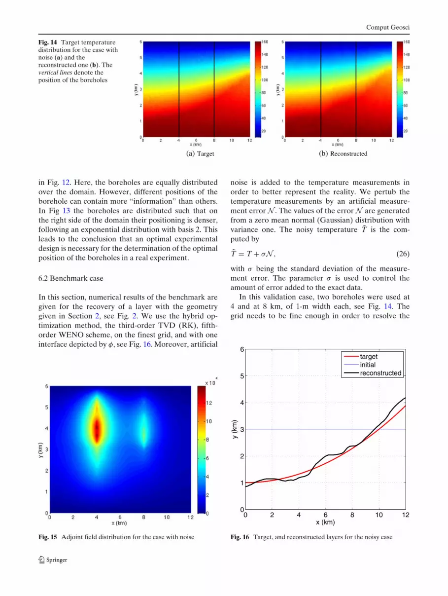
Fig. 14 Target temperaturedistribution for the case withnoise (a) and thereconstructed one (b). Thevertical lines denote theposition of the boreholes
(a) Target (b) Reconstructed
in Fig. 12. Here, the boreholes are equally distributedover the domain. However, different positions of theborehole can contain more “information” than others.In Fig 13 the boreholes are distributed such that onthe right side of the domain their positioning is denser,following an exponential distribution with basis 2. Thisleads to the conclusion that an optimal experimentaldesign is necessary for the determination of the optimalposition of the boreholes in a real experiment.
6.2 Benchmark case
In this section, numerical results of the benchmark aregiven for the recovery of a layer with the geometrygiven in Section 2, see Fig. 2. We use the hybrid op-timization method, the third-order TVD (RK), fifth-order WENO scheme, on the finest grid, and with oneinterface depicted by φ, see Fig. 16. Moreover, artificial
Fig. 15 Adjoint field distribution for the case with noise
noise is added to the temperature measurements inorder to better represent the reality. We pertub thetemperature measurements by an artificial measure-ment error N . The values of the error N are generatedfrom a zero mean normal (Gaussian) distribution withvariance one. The noisy temperature T is the com-puted by
T = T + σN , (26)
with σ being the standard deviation of the measure-ment error. The parameter σ is used to control theamount of error added to the exact data.
In this validation case, two boreholes were used at4 and at 8 km, of 1-m width each, see Fig. 14. Thegrid needs to be fine enough in order to resolve the
x (km)
y (k
m)
0 2 4 6 8 10 120
1
2
3
4
5
6targetinitialreconstructed
Fig. 16 Target, and reconstructed layers for the noisy case

Comput Geosci
borehole, which leads to huge grids in the benchmarkcase where the domain is in the order of km. Noise wasadded to the measured temperature according to Eq. 26with standard deviation σ = 1. The target temperaturedistribution for σ = 1 and the recovered temperaturefield are shown in Fig. 14. The adjoint field distributionis shown in Fig. 15 for the first iteration. One can clearlysee the positions of the boreholes which act as “sourceterm” in the adjoint equation. The target layer, togetherwith the initial and the reconstructed ones are givenin Fig. 16. As it can be seen from the temperaturedistributions the errors are small, the objective functionhas also decreased significantly, and the recovered layerrepresents quite well the target geometry.
7 Conclusions and outlook
In this paper, we have presented a numerical methodfor the computation of the geometry of geophysical lay-ers from temperature measurements. The problem fallsunder the category of inverse problems and methodsof shape optimization have been used to identify theunknown layers. The “speed method” together with theadjoint formulation is used for the calculation of theshape sensitivities. The unknown geometry is describedwith the help of the level set function. The identificationapproach is based on an iterative gradient descentmethod. This leads to a set of adjoint equations and anonlinear Hamilton–Jacobi type equation for the evo-lution of the boundaries of the layers. These equationstogether with the forward model for the geothermicflow have to be solved subsequently. Note that even ifthe original model depends in a nonlinear way on theconductivity and permeability tensors the adjoint equa-tions are linear in the unknowns. However, in order tocompute the solution to the adjoint equation, the for-ward solution on the full grid in space and time has tobe known. In particular, for time-dependent problemsthis may pose serious computational challenges.
A first extension of the presented method involvesconsidering all physical properties depending on theunknown shape. This, of course, will change the adjointequations and the gradient derivative. Furthermore,in the objective function pressure measurements canbe included in addition to temperature, which willalso yield additional terms to the adjoint and gradientequation. The calculus deriving the adjoint equationsincluding hydraulic permeability can be found in [38].
In the present work, the physical properties of thedifferent zones have been considered known a priori.A question that has to be answered in the future is howto identify both the shape and the physical properties
Fig. 17 A 3D grid with different property zones described by asurface level set function
of the geophysical layers from flow or heat measure-ments. In this case, shape reconstruction methods andparameter identification techniques have to be com-bined for the joint identification. A modification of thealgorithm would include a further optimization proce-dure, performed either outside or inside the presentoptimization loop, for the identification of the unknownconductivities.
A straight-forward generalization of the presentmethod is the application to 3D case. The zero contourof the level set function would then be a surface in the3D space representing the interface of the geologicallayers, see for example Fig. 17. Another extension ofthe level set function is the description of layers withmore than two material properties. This can be donewith the use a more than one level set functions asshown in Fig. 18 (see for example [59] for structuraloptimization). The different material zones of Fig. 18
1
2
3
4
5
6
unit #
0 2000 4000 6000 8000 10000 12000
x(m)
0
2000
4000
6000
y(m
)
Fig. 18 Multiple level set functions for the characterization ofmultiple physical materials

Comput Geosci
would then be defined with the help of six-level setfunctions, in the following shown for the first and thelast zone:
�1 = {φ1 > 0, φ5 > 0} ∪ {φ1 > 0, φ6 < 0}, (27a)
�6 = {φ4 < 0, φ5 > 0} ∪ {φ2 < 0, φ6 < 0}, (27b)
with D =6⋃
i=1
�i and �i ∩ � j = ∅, i �= j. Note that the
number of level set functions does not necessarilydefine the number of different parameter zones. A sim-ilar approach for identifying different material zones isthe truncated pluri-Gaussian method by [27].
On the optimization part, the simple steepest de-scent algorithm used here can be substituted by quasi-Newton methods, which require only the gradient ofthe objective function, and can reduce the number ofrequired iterations until convergence has achieved.
Regarding regularization a lot of open questions stillremain; first is the application of different criteria suchas GCV and L-curve in order to estimate the optimalregularization parameter. Further questions involve thesmoothing of the interface; by interpolating, or evenapproximating, the zero contour of the interface ad-ditional smoothing can be applied. The interaction ofthis kind of smoothing, together with the regularizationitself and the reparametrization of the level set is stillan open problem.
The present study represents a first step towardsthe development of corresponding methods for mul-tiphysics investigations, e.g., in geothermal reservoirs,where multiphase fluid flow is an important compo-nent. The necessary generalizations of our method re-main a challenging task for the future.
Acknowledgments This work was supported by the BMBFproject MeProRisk, TP AM, “Identifizierung von Schichtgren-zen für Geothermie”, DAAD D/08/110276, 50727872 and DFGHE5386/8-1. VR was funded by the Ramón y Cajal Program ofthe Spanish Ministry for Science and Education. The authorsacknowledge the reviewers for reading the manuscript very care-fully and providing constructive comments.
Appendix A: Adjoint equation
A sample term for the adjoint equation is going tobe calculated. First, the Fréchet derivative have to beintroduced. Let F be a continuous nonlinear operatorF : U → V acting between the Banach spaces U andV . Then the directional derivative of F at a point u indirection v is defined as
dF(u; v) := limτ↓0
F(u + τv) − F(u)
τ= f ′
v(τ )
∣∣∣τ=0
if the limit on the right-hand side exists. If the direc-tional derivatives dF(u; v) exist for all v ∈ U and in ad-dition dF(u, ·) : U → V is a continuous linear operator,the F is called Fréchet-differentiable at u with Fréchet-derivative
F ′(u)v := dF(u; v) ∀v ∈ U .
As an example we consider the time-dependent term,see Eq. 6, F = ∫ t1
0
∫�(ρc)eθT dxdt = ∫ t1
0 (θ, Tt)edt. Tak-ing its Frechet derivative, we have:
dLt(T; η) = limτ↓0
∫ t10 (θ, (T + τη)t)edt − ∫ t1
0 (θ, Tt)edt
τ
where η ∈ {H1(D)∣∣ η(·, t)=0 on �D and η(·, 0) = 0 on
D)} is the variation of temperature with homogeneousboundary and initial conditions. Then, after expandingthe time derivative and the bilinear form we have
dLt(T; η) = limτ↓0
∫ t10 (θ, τηt)edt
τ=
∫ t1
0(θ, ηt)edt.
By applying integration by parts for the time derivativewe get
dLt(T; η) = −∫ t1
0(η, θt)edt +
∫D(θη)
∣∣t10 (ρc)edx.
Since η(·, 0) = 0, it follows from the second term thatθ(·, t1) = 0, i.e., the “initial” condition is moved to thefinal time. Also, in the first term the sign has beeninverted; this leads to solving the adjoint equation“backwards” in time. The derivatives for the rest termsof the Lagrange function can be derived in a similarway.
Appendix B: Gradient equation
Here follows briefly the calculation of the shape gradi-ents. In the Lagrange function (9), the only two termsthat depend on the shape � is the one containing thethermal conductivity λe, which is a volume integralwith no PDE constraints (remember that the PDEconstraints have been transformed with the help of theLagrange multipliers) and the regularization term. Wefirst give the Hadamard formula for volume and surface

Comput Geosci
integrals. For a general volume function, f : � → R,not depending on a PDE constraint, i.e.,
J(�) =∫
�
f dA,
the shape derivative and the shape gradient are gi-ven by
d J(�)[V] =∫
�
V · nf dS. (28)
For a general surface function, g : T(∂�) → R such that∂g∂n exists,
J(ω) =∫
∂�
g d�
the shape derivative and shape gradient are given by
d J(�)[V] =∫
∂�
V · n[
∂g∂n
+ κg]
d�,
where κ is the additive mean curvature of ∂�. Proofs ofthe above lemmata can be found in [55]. This calculuswill be applied to L given by Eq. 9. The derivative ofthe Lagrangian can be given by
dL(�)[V] = d�
∫ t1
0aλe(θ, T)dt + ε d�
∫∂�
Rd�
= d�
∫ t1
0
∫D
λe∇θ · ∇Tdxdt + ε d�
∫∂�
Rd�.
By splitting the domain of the first term into � andD\� where λe is constant, and applying the lemma forsurface derivatives we get:
dL(�)[V]
= d�
∫ t1
0
(∫�
λe∇θ · ∇Tdx +∫
D\�λe∇θ · ∇Tdx
)dt
+ ε
∫∂�
V · n[∂R∂n
+ κR]
d�
= d�
∫ t1
0
(∫�
λ1∇θ · ∇Tdx +∫
D\�λ2∇θ · ∇Tdx
)dt
+ ε
∫∂�
V · n[∂R∂n
+ κR]
d�
= d�
∫ t1
0
(∫�
λ1∇θ · ∇Tdx +∫
Dλ2∇θ · ∇Tdx
−∫
�
λ2∇θ · ∇Tdx)
dt
+ ε
∫∂�
V · n[∂R∂n
+ κR]
d�,
which leads to
dL(�)[V]
= d�
∫ t1
0
(∫�
(λ1 − λ2)∇θ · ∇Tdx+∫
Dλ2∇θ · ∇Tdx
)dt
+ ε
∫∂�
V · n[∂R∂n
+ κR]
d�.
In the second term of the last formula, neither D norλ2 depends on �, so the derivative is zero. By usingHadamard’s formula on the remaining first term, theshape derivative is:
dL(�)[V] =∫ t1
0
∫∂�
(λ1 − λ2)∇θ · ∇T V · n d�dt
+ ε
∫∂�
V · n[∂R∂n
+ κR]
d�. (29)
Notice that the whole derivative of the volume andsurface integrals is now condensed on the boundary ofthe shape.
References
1. Allaire, G., Jouve, F., Toader, A.: Structural optimizationusing sensitivity analysis and a level-set method. J. Comput.Phys. 194, 363–393 (2004)
2. BenAmeur, H., Burger, M., Hackl, B.: Level set methods forgeometric inverse problems in linear elasticity. Inverse Probl.20, 673–696 (2004)
3. Berg, J., olmström, K.: On parameter estimation using levelsets. SIAM J. Control Optim. 37, 1372–1393 (1999)
4. Borsic, A., Graham, B.M., Adler, A., Lionheart, W.R.B.: In-vivo impedance imaging with total vatation regularization.IEEE Trans. Med. Imag. 29(1), 44–54 (2010)
5. Burger, M.: A level set method for inverse problems. InverseProbl. 17, 1327–1355 (2001)
6. Burger, M.: A framework for the construction of level-setmethods for shape optimization and reconstruction. Inter-faces Free Bound. 5, 301–329 (2003)
7. Burger, M., Hackl, B., Ring, W.: Incorporating topologicalderivatives into level set methods. J. Comput. Phys. 194, 344–362 (2004)
8. Burger, M., Osher, S.: A survey on level set methods forinverse problems and optimal design. Eur. J. Appl. Math. 16,263–301 (2005)
9. Cardiff, M., Kitanidis, P.: Bayesian inversion for facies detec-tion: an extensible level set framework. Water Resour. Res.45, W10416 (2009)
10. Chan, T., Tai, X.-C.: Identification of discontinuous coef-ficients in elliptic problems using total variation regulariza-tion. SIAM J. Sci. Comput. 25(3), 881–904 (2003)
11. Chan, T., Tai, X.-C.: Level set and total variation regu-larization for elliptic inverse problems with discontinuouscoefficients. J. Comput. Phys. 193, 40–66 (2003)
12. Chung, E., Chan, T., Tai, X.-C.: Electrical impedance to-mography using level set representation and total variationregularization. J. Comput. Phys. 205, 357–372 (2005)

Comput Geosci
13. H.Diersch, J.-G., Kolditz, O.: Variable-density flow andtransport in porous media: approaches and challenges. Adv.Water Resour. 25, 899–944 (2002)
14. Donea, J., Huerta, A.: Finite element methods for flow prob-lems. Wiley, New York (2003)
15. Dorn, O., Lesselier, D.: Level set methods for inverse scatter-ing. Inverse Probl. 22, R67–R131 (2006)
16. Dorn, O., Lesselier, D.: Level set methods for inversescattering—some recent developments. Inverse Probl. 25,125001 (2009)
17. Dorn, O., Miller, E., Rappaport, C.: A shape reconstructionmethod for electromagnetic tomography using adjoint fieldsand level sets. Inverse Probl. 16, 1119–1156 (2000)
18. Farquharson, C.G.: Constructing piecewise-constant mod-els in multidimensional minimum-structure inversions. Geo-physics 73(1), K1–K9 (2008)
19. Fedkiw, R., Aslam, T., Merriman, B., Osher, S.: A non-scillatory eulerian approach to interfaces in multimaterialflows (the ghost fluid method). J. Comput. Phys. 152, 457–492(1999)
20. Giles, M., Pierce, N.: An introduction to the adjoint approachto design. Flow Turbul. Combust. 65, 393–415 (2000)
21. Hughes, T.: The finite element method: linear static anddynamic finite element analysis. Prentice-Hall, EnglewoodCliffs (1987)
22. Hysing, S., Turek, S.: The Eikonal equation: numericalefficiency vs. algorithmic complexity on quadrilateral grids.In: Proceedings of ALGORITMY, pp. 22–31 (2005)
23. Ito, K., Kunisch, K., Li, Z.: Level-set function approach toan inverse interface problem. Inverse Probl. 17, 1225–1242(2001)
24. Kolditz, O.: Non-linear flow in fractured rock. Int. J. Numer.Methods Heat Fluid Flow 11(6), 547–575 (2001)
25. Kolditz, O., Ratke, R., H.-Diersch, J.G., Zielke, W.: Coupledgroundwater flow and transport: 1. Verification of variabledensity flowand transport models. Adv. Water Resour. 21,21–46 (1998)
26. Litman, A., Lesselier, D., Santosa, F.: Reconstruction of atwo-dimensional binary obstacle by controlled evolution ofa level-set. Inverse Probl. 14, 685–706 (1998)
27. Liu, N., Oliver, D.: Ensemble kalman filter for automatichistory matching of geologic facies. J. Pet. Sci. Eng. 47, 147–161 (2005)
28. Mitchell, I.: The flexible, extensible and efficient toolbox oflevel set methods. J. Sci. Comput. 35, 300–329 (2008)
29. Nelder, J., Mead, R.: A simplex method for function mini-mization. Comput. J. 7, 308–313 (1965)
30. Neuman, S., Carrera, J.: Maximum-likelihood adjoint-statefinite-element estimation of groundwater parameters understeady- and nonsteady-state conditions. Appl. Math. Comput.17, 405–432 (1985)
31. Nicolai, M.: Towards shape optimization for fluids involv-ing complex shape parametrization. In: SIAM Conferenceon Computational Science and Engineering (CSE09), Miami,vol. 2 (2009)
32. Nocedal, J., Wright, S.J.: Numerical Optimization. Springer,New York (1999)
33. Oliver, D., Chen, Y.: Recent progress on reservoir historymatching: a review. Comput. Geosci. 15(1), 185–221(2010)
34. Oliver, D.S., Reynolds, A.C., Liu, N.: Inverse theory forpetroleum reservoir characterization and history matching.Cambridge University Press, Cambridge (2008)
35. Osher, S., Fedkiw, R.: Level set methods: an overview andsome recent results. J. Comput. Phys. 169, 463–502 (2001)
36. Osher, S., Santosa, F.: Level set methods for optimizationproblems involving geometry and constraints I. Frequencies
of a two-density inhomogeneous drum. J. Comput. Phys. 171,272–288 (2001)
37. Osher, S., Sethian, J.: Fronts propagating with curvature-dependent speed: algorithms based on Hamilton–Jacobi for-mulations. J. Comput. Phys. 79, 12–49 (1988)
38. Papadopoulos, D.: Quantification of concentration measure-ments in multicomponent systems with NMR. Ph.D. thesis,RWTH Aachen University (2011)
39. Pilkinkton, M.: 3D magnetic data-space inversion withsparseness constraints. Geophysics 74, L7–L15 (2009)
40. Plessix, R.: A review of the adjoint-state method for comput-ing the gradient of a functional with geophysical applications.Geophys. J. Int. 167, 495–503 (2006)
41. Poeter, E., Hill, M.: Inverse models: a necessary next step inground-water modeling. Ground Water 2, 250–260 (1997)
42. Portniaguine, O.: Image focusing and data compression inthe solution of geophysical inverse problems. Ph.D. thesis,University of Utah (1999)
43. Probst, M., Lülfesmann, M., Nicolai, M., Bücker, M., Behr,M., Bischof, C.: Sensitivity of optimal shapes of artificialgrafts with respect to flow parameters. Comput. MethodsAppl. Mech. Eng. 199, 997–1005 (2010)
44. Ramananjaona, C., Lampert, M., Lesselier, D.: Shape inver-sion from TM and TE real data by controlled evolution oflevel sets. Inverse Probl. 17, 1585 (2001)
45. Ramananjaona, C., Lampert, M., Lesselier, D.: Shape recon-struction of buried obstacles by controlled evolution of a levelset: from a min–max formulation to numerical experimenta-tion. Inverse Probl. 17, 1087–1112 (2001)
46. Rath, V., Mottaghy, D.: Smooth inversion for ground surfacetemperature histories: estimating the optimum regularizationparameter by generalized cross-validation. Geophys. J. Int.171(3), 1440 (2007). doi:10.1111/j.1365–246X.2007.03587.x
47. Rath, V., Wolf, A., Bücker, H.-M.: Joint three-dimensionalinversion of coupled groudwater flow and heat transferbased on automatic differentiation: sensitivity calculation,verification, and synthetic examples. Geophys. J. Int. 167(1),453–466 (2006)
48. Rodgers, C.D.: Inverse methods for atmospheric sounding.World Scientific, Singapore (2000)
49. Santosa, F.: A level set approach for inverse problems involv-ing obstacles. ESAIM Control Optim. Calculus Var. 1, 17–33(1996)
50. Schweiger, M., Dorn, O., Zacharopoulos, A., Nissila, I.,Arridge, S.R.: 3d level set reconstruction of model and ex-perimental data in diffuse optical tomography. Opt. Express18(1), 150–164 (2010)
51. Sethian, J.: Theory, algorithms and applications of level setmethods for propagating interfaces. Acta Numer. 5, 309–395(1996)
52. Sethian, J.: Level set methods and fast marching methods.Evolving interfaces in computational geometry, fluid me-chanics, computer vision, and materials science. CambridgeUniversity Press, Cambridge (1999)
53. Sethian, J., Wiegmann, A.: Structural boundary design vialevel set and immersed interface methods. J. Comput. Phys.163, 489–528 (2000)
54. Sirkes, Z., Tziperman, E.: Finite difference of adjoint or ad-joint of finite difference? Mon. Weather Rev. 125(12), 3373–3378 (1997)
55. Sokolowski, J., Zolesio, J.-P.: Introduction to shape optimiza-tion. Shape sensitivity analysis. Springer, New York (1992)
56. Tarantola, A.: Inverse problem theory. Methods for modelparameter estimation. SIAM, Philadelphia. http://www.ipgp.jussieu.fr/∼tarantola/Files/Professional/Books/index.html(2005)

Comput Geosci
57. Tröltzsch, F.: Optimale Steuerung Partieller Differentialglei-chungen: Theorie, Verfahren und Anwendungen. Vieweg,Weisbaden (2005)
58. Villegas, R., Dorn, O., Moscoso, M., Kindelan, M.: Simul-taneous characterization of geological regions and para-meterized internal permeability profiles in history match-ing. In: Proceedings of the 10th European conference onthe mathematics of oil recovery, Amsterdam, p. A015(2006)
59. Wang, M., Wang, X.: Color level sets: a multi-phase levelset method for structural topology optimization with multiplematerials. Comput. Methods Appl. Mech. Eng. 193, 469–496(2004)
60. Wang, M., Wang, X., Guo, D.: A level set method for struc-tural topology optimization. Comput. Methods. Appl. Mech.Eng. 192, 227–246 (2003)
61. Zhdanov, M.S.: Geophysical inverse theory and regulariza-tion problems. Elsevier, Amsterdam (2002)