Discrete contours in multiple views: approximation and recognition

Discrete contours in multiple views: approximation and recognition

M. Pawan Kumar, Saurabh Goyal, Sujit Kuthirummal, C.V. Jawahar*, P.J. Narayanan

Centre for Visual Information Technology, International Institute of Information Technology, Gachibowli, Hyderabad 500 019, India

Received 20 February 2003; received in revised form 13 January 2004; accepted 17 March 2004

Abstract

Recognition of discrete planar contours under similarity transformations has received a lot of attention but little work has been reported on

recognizing them under more general transformations. Planar object boundaries undergo projective or affine transformations across multiple

views. We present two methods to recognize discrete curves in this paper. The first method computes a piecewise parametric approximation

of the discrete curve that is projectively invariant. A polygon approximation scheme and a piecewise conic approximation scheme are

presented here. The second method computes an invariant sequence directly from the sequence of discrete points on the curve in a Fourier

transform space. The sequence is shown to be identical up to a scale factor in all affine related views of the curve. We present the theory and

demonstrate its applications to several problems including numeral recognition, aircraft recognition, and homography computation.

q 2004 Elsevier B.V. All rights reserved.

Keywords: Planar shape recognition; Polygonal approximation; Fourier transform; Invariant; Projective geometry; Piecewise conic approximation

1. Introduction

Analysis of multiple views of the same scene is an area of

active research in computer vision today. The study of the

structure of projections of points and lines in two views

received much attention in the 1980s and early 1990s [1–3].

Similar study on the projections of points and lines in three

and more views followed since then [3–5]. These multi-

view studies have concentrated on how geometric primi-

tives like points, lines and planes are related across views.

Specifically, the algebraic constraints satisfied by the

projections of such primitives in different views have been

the focus of intense studies. Discrete contours formed by

boundaries of objects are of great interest for shape

recognition. The contour consists of an ordered sequence

of points. While projection of each point satisfies multi-

view constraints separately, their sequence can have

additional constraints that can help in recognizing them

under multiple views.

We study the issues in recognizing discrete planar

contours, consisting of a sequence of points, in multiple

views under different projection models in this paper. We

limit the recognition problem to planar objects represented

using their discrete boundaries. Planar shape recognition has

been studied well. Recognition by alignment [6], polygonal

approximation [7], based on geometrically invariant fea-

tures [8], linear combination of models [9], etc. have

appeared in the literature. Descriptors computed in the

Fourier domain [10] have also been used for recognition.

These algorithms work well for similarity transformations

between views. The image-to-image transformation is more

general in practical situations of interest. When a planar

object is imaged from multiple viewpoints using a

perspective camera, its images are generally related by a

projective homography. In many practical situations, the

homography is close to be an affine. For both affine and

projective cases, conventional algorithms, designed for

similarity transforms, will not be enough.

The problem of shape recognition in the context of

multiple views can be posed thus. Given the image of an

object in one or more views, can we recognize them to be

images of the same object when the viewing parameters of

the cameras are unknown.

Projective and affine invariants for points, lines and

parametric and algebraic curves, such as conics, have been

discovered [11]. Discrete contours, not amenable to simple

algebraic or parametric representations, pose new problems

and have not been studied much earlier. Differential

invariants that require higher order derivatives of contours

have been used [11,12]. Subsequently integrals involving

0262-8856/$ - see front matter q 2004 Elsevier B.V. All rights reserved.

doi:10.1016/j.imavis.2004.03.022

Image and Vision Computing 22 (2004) 1229–1239

www.elsevier.com/locate/imavis

* Corresponding author.

E-mail address: [email protected] (C.V. Jawahar).

http://www.elsevier.com/locate/imavis

differentials of image curves have been used successfully in

recognition systems [13]. Another relevant effort identifies a

set of affine invariant features and uses them for recognition

[14] in a classical pattern recognition framework.

In this paper, we present two approaches for the

recognition of discrete planar contours in multiple views.

The first approach is inspired by polygonal approximation

techniques [7]. We propose a polygonal approximation

algorithm for an invariant characterisation of a contour

under projective transformation. We extend it to piecewise

parametric approximation of the discrete contour. The

specific parametric structures used are lines, resulting in a

polygonal approximation, and conics. We show how the

multi-view invariants of the underlying parametric structure

can be exploited to devise a projective invariant piecewise

parametric approximation. Thus, the approximation com-

puted from multiple views of the contour will be isomorphic

to each other. This necessary condition satisfied by

matching contours can be used for recognizing its shape

in multiple views without explicit correspondence between

points.

The second approach uses new contour invariants

computed from the sequence of points on the contour.

This approach combines multi-view constraints on corre-

sponding points and the Fourier domain constraints of the

sequence of points. We achieve their fusion in a Fourier

domain representation of the point sequence. We show that

the novel Fourier vector representation of the contour points

yields a single-view invariant sequence k that is identical up

to a scale factor for all affine-related projections of the

contour. This can be the basis for recognizing the shape in

multiple views. This is a direct method for recognition that

does not involve the selection of starting points or

approximation of the contour using parametric structures.

We establish the contour invariants for affine homographies,

but show that they are satisfied for most practical situations

when the image-to-image homography is not strictly affine.

We present a general contour invariant in this paper. In a

previous work, we have shown that recognition constraints

based on the magnitude and phases of the Fourier vector

representation also exist [15].

Section 2 presents the basic problem formulation and

establishes the notation used throughout this paper. Section

3 discusses the general theory behind projective invariant

piecewise parametric representation of discrete contours.

The Fourier domain contour invariant is presented in

Section 4. We establish the affine invariant and present

the multi-view recognition condition as a rank constraint on

a measurement matrix. Section 5 shows that the problem of

recognizing polygonal shapes in multiple views can be

solved using the Fourier domain invariant on a sequence of

lines in the dual space. Section 6 shows the results of

applying both approaches for contour recognition on a

number of applications involving the recognition of

numerals and aircraft silhouettes. We also show the

extension of the recognition scheme to compute point-wise

correspondence between matching contours and then to

compute the homography between a pair of views. Section 7

presents a few concluding remarks.

2. Problem formulation

Let O be a set of N points on the boundary of a planar

object imaged in multiple views. Let ðul½i�; vl½i�;wl½i�Þ be the

homogeneous coordinates of points on the image of the

closed boundary in view l: This boundary is represented by a

sequence of vectors as shown below

xl½i� ¼

ul½i�

vl½i�

wl½i�

26664

37775

When a planar object is imaged from multiple viewpoints,

points on it undergo a transformation that can be

mathematically described as a general projective transform-

ation, which is a linear operation (3 £ 3 matrix) in

homogeneous coordinates

xl½i� ¼ Mlx0½i� ð1Þ

In some special cases, additional constraints on Ml can

result in affine or similarity transformation.

Two views are related by a similarity transformation only

when there is a rotation, and/or a translation, and/or a

uniform scaling between them. Most reported recognition

algorithms are primarily designed to handle similarity

transformations. However, affine transformations deform

the shape of an object beyond rigid motions though they do

preserve parallelism and points at infinity. An affine

homography between two images is represented by a Ml

matrix with its last row as ½0 0 1�: Affine transformations

form a subset of the general projective group.

Projective transformations, in general, do not preserve

parallelism of lines and can map points at infinity to finite

points and vice versa. It has been shown that a planar object

viewed from multiple viewing positions results in a

projective image-to-image homography [3]. However, for

cases like narrow field of view or imaging an object from a

distance, an affine transformation is considered to be a good

approximation of the projective transformation.

As we go higher up in the hierarchy of transformations

(similarity , affine , projective) the constructs that are

preserved (remain invariant) become fewer, making the task

of recognition more challenging. We address the problem of

planar object recognition using appropriate invariants.

2.1. Invariants

Let p be a parameter vector subject to the linear

transformation Ml: A scalar invariant IðpÞ of p is preserved

under the transformation if IðplÞ ¼ Iðp0Þ [11]. Here, IðplÞ is

M. Pawan Kumar et al. / Image and Vision Computing 22 (2004) 1229–12391230

the function of the parameters after the linear transform-

ation. If the transformation Ml is affine, the invariants are

called affine invariants. For example, ratio of areas and ratio

of lengths on parallel lines are invariant to affine

transformations. Several cross-ratios are invariant under

projective transformation. Cross-ratio of four collinear

points is defined as the ratio of ratios of distances between

points. Below we describe the cross-ratios that we employ,

namely cross-ratio of areas and concurrent lines.

Cross-ratio of areas of five points. The cross-ratio of the

areas of five points x1; x2; x3; x4; and x5 is defined by

crðx1; x2; x3; x4; x5Þ ¼Dx1x2x5

Dx3x4x5

Dx1x3x5Dx2x4x5

; ð2Þ

where Dxixjxkis the area of the triangle formed by points

xi; xj; xk: This is invariant to general linear or projective

transformations [11].

Cross-ratio of four concurrent lines. The cross-ratio of

four concurrent lines l1; l2; l3; l4 is defined as

crðl1; l2; l3; l4Þ ¼sin u13 sin u24

sin u23 sin u14

; ð3Þ

where uij represents the angle formed by the lines li and lj:

This is invariant to a general projective transformation [11].

We employ these invariances for piecewise parametric

approximation of discrete contours.

3. Projectively invariant piecewise parametric

representation

Parametric representation is a popular method for

providing a compact representation of planar contours. A

piecewise parametric representation of a contour partitions

the points on the contour into sets, and represents each set

with the help of a few parameters. One example of such a

representation is polygonal approximation. This has been

extensively used as an intermediate step in various

applications such as planar shape recognition, volume

rendering and multi-resolution modeling [16–18].

Polygonal approximation may be achieved by mini-

mizing the error in approximation. A general optimization

of the objective function may be computationally

expensive and prone to get stuck in local minima. Most

popular polygonal approximation algorithms look for an

optimal solution using a greedy algorithm [7,19]. Some of

these algorithms are designed for fast approximation.

They, in general, exploit the connectedness and ordering

of the points in the set. There are also algorithms that do

not exploit the connectedness of points [20]. They group

points on the boundary into linear clusters. Some other

algorithms emphasize the optimality and efficiency of the

polygonal approximation [21]. Conic sections are also

often used as the parametric representation for each

partition [22].

Let xl½i�; i ¼ 1; 2;…; n be a set of points on the boundary

of a planar object to be approximated using parametric

sections in the lth view. These sequences in multiple views

are related by xl½i� ¼ Mlx0½i�: In individual views, these

boundary sequences can be approximated into k mutually

exclusive and collectively exhaustive subsets fl1;…;fl

k

such that each of the subsets can be approximated using a

few parameters. This can be achieved by minimizing an

objective function of the form

Jl ¼Xlfl

jl

i¼1

dðxl½i�;QljÞ; xl½i� [ fl

j ð4Þ

where Qlj is the parametric structure which approximates the

points in flj and dð·Þ is a measure of separation of xl½i� from

Qlj: The separation dð·Þ can be the distance along the normal

or a measure of how the parametric structure Qlj distorts the

real point xl½i�: For the parametric representation to be

invariant to projective transformations, there should be a

one-to-one mapping from fli to f0

i :

We now show that as long as we can identify a projective

invariant which gives a measure of separation for the desired

parametric structure, we can find an algorithm to represent

the curve using that parametric structure. We discuss two

specific cases of this approach in the form of polygonal

approximation and piecewise conic section approximation.

3.1. Proposed approach

The existence of a projectively invariant piecewise

parametric method depends on the availability of a

projective invariant which can give a measure of separation

of a point from the desired parametric structure. Let IðpÞ be

a projective invariant for a set of points p and let Iðx½i�Þ

denote its value when all points of p except x½i� are kept

fixed. If the locus of x½i� for which Iðx½i�Þ ¼ k is a

parametric structure Q; we can use lIðx½i�Þ2 kl as a

measure of separation. We first select the fixed points and

compute the invariants corresponding to those points. We

then move along the contour until the approximation error is

sufficiently large. Thus, we can identify regions in the curve

which can be approximated using a parametric structure.

3.2. Projective invariant polygon approximation

In this section, we describe an algorithm that can result in

isomorphic polygonal approximation for projectively trans-

formed versions of the same image. Some preliminary

results of this have been presented in Ref. [16].

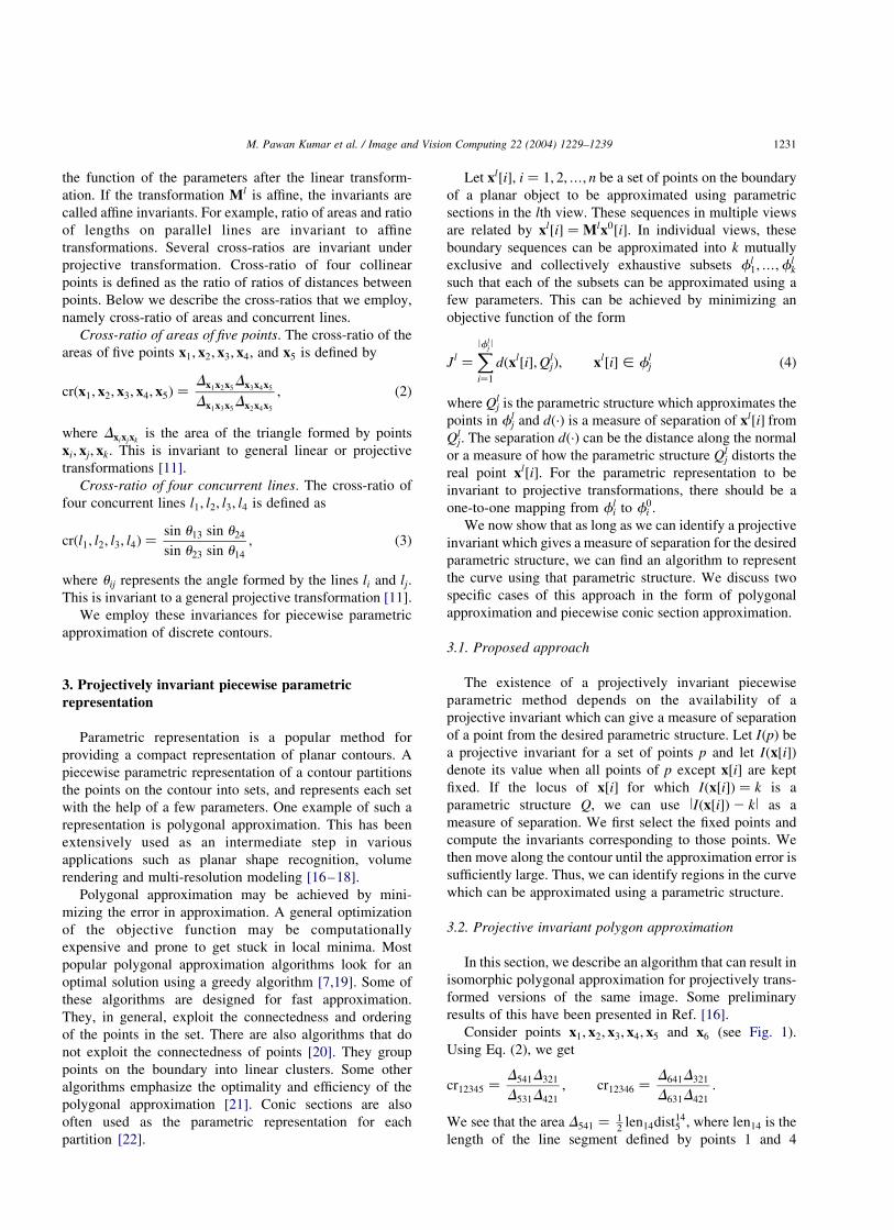
Consider points x1; x2; x3; x4; x5 and x6 (see Fig. 1).

Using Eq. (2), we get

cr12345 ¼D541D321

D531D421

; cr12346 ¼D641D321

D631D421

:

We see that the area D541 ¼ 12

len14dist145 ; where len14 is the

length of the line segment defined by points 1 and 4

M. Pawan Kumar et al. / Image and Vision Computing 22 (2004) 1229–1239 1231

and dist145 is the perpendicular distance of point 5 from the

line defined by points 1 and 4. Now we consider the ratio of

cross-ratios [11,16] as

l ¼cr12345

cr12346

¼D541D631

D531D641

¼len14dist14

5 len13dist136

len13dist135 len14dist14

6

¼dist14

5 =dist135

dist146 =dist13

6

: ð5Þ

We first establish three useful properties before proving the

existence of projective invariant polygon approximation.

Property 1. An invariant polygonal approximation algor-

ithm can exist only for a transformation where collinearity

is preserved. To verify this, we assume that we have a

polygonal approximation algorithm invariant to a trans-

formation which does not preserve collinearity. Under

such a transformation, not every line gets transformed as

a line. From this it is clear that there cannot exist

a polygonal approximation algorithm which is

invariant to such a transformation. Since projective

transformation preserves collinearity, there can exist a

polygonal approximation algorithm invariant to this

transformation.

Property 2. The ratio of cross-ratios of areas gives us a

measure of deviation dð·Þ for polygonal approximation. This

is true as Eq. (5) shows that l can be interpreted as the ratio

of the ratio of perpendicular distances of the points x5 and

x6 from the two lines line13 and line14: This value equals 1

for the line line15: When the point x6 moves away from this

line, l moves away from 1. Thus, l gives a measure of the

collinearity of the points x1; x5 and x6: The measure dð·Þ ¼

ll2 1l can then be used as the measure of deviation as

given in Eq. (4).

Property 3. The ratio of cross-ratios of area ðlÞ is

invariant to projective transformations since the cross-

ratios of areas are projectively invariant.

Therefore, there exists an algorithm for polygonal

approximation which is invariant to projective transform-

ation as it is clear that there is a function dð·Þ which is

invariant to projective transformation. This would result in a

one-to-one mapping between the subsets ðf1;f2;…;fkÞ:

We develop the algorithm in the following manner.

(1) Choose point 1 as the starting point and point 5 as the

point next to point 1 on the curve. Points 2, 3, and 4

may or may not lie on the curve.

(2) Choose the point adjacent to 5 on the curve as point 6.

Measure dð6Þ ¼ llð6Þ2 1l:(3) If dð6Þ , t (a suitable tolerance threshold), move point

6 forward. Go to step 2.

(4) Otherwise, approximate the curve by the line segment

joining points 1 and 6. Set point 6 as the new point 1.

Go to step 1.

The algorithm described above was implemented to work

with real images. Points 3, 4, and 5 have to be chosen

carefully in order to overcome errors that are present in real

images. The most prominent error is due to the discretiza-

tion of the curve because of which the cross-ratios

calculated may differ in different views [11]. In order to

decrease the effect of discretization, points 3, 4 and 5 were

chosen far apart from each other so that the areas to be

calculated for l were large. This prevents a small change in

the locations of points 3, 4 or 5 to affect the cross-ratios

noticeably. Point 5 need not be the same in multiple views

of the same object as long as it is close to point 1. This is

because the contours are smooth, so we can assume that

points within a small distance from point 1 are almost

collinear and hence give the same value for l:

The reference points should not be collinear in which

case the cross-ratio of areas will be undefined. Another

problem that arises is obtaining points 3 and 4 which

correspond in different views. An affine or euclidean

invariant heuristic to obtain these points can be used

which leads to slight differences in the positions of points 3

and 4. In most real images, if the threshold is kept low,

differences in the positions of points 3 and 4, change the

locations of boundary points by only 1–2 pixels. The choice

of the threshold should depend on the curvature of the

section that we are trying to approximate. For example, for a

linear section the threshold should be low to retrieve the

same linear section as the approximation.

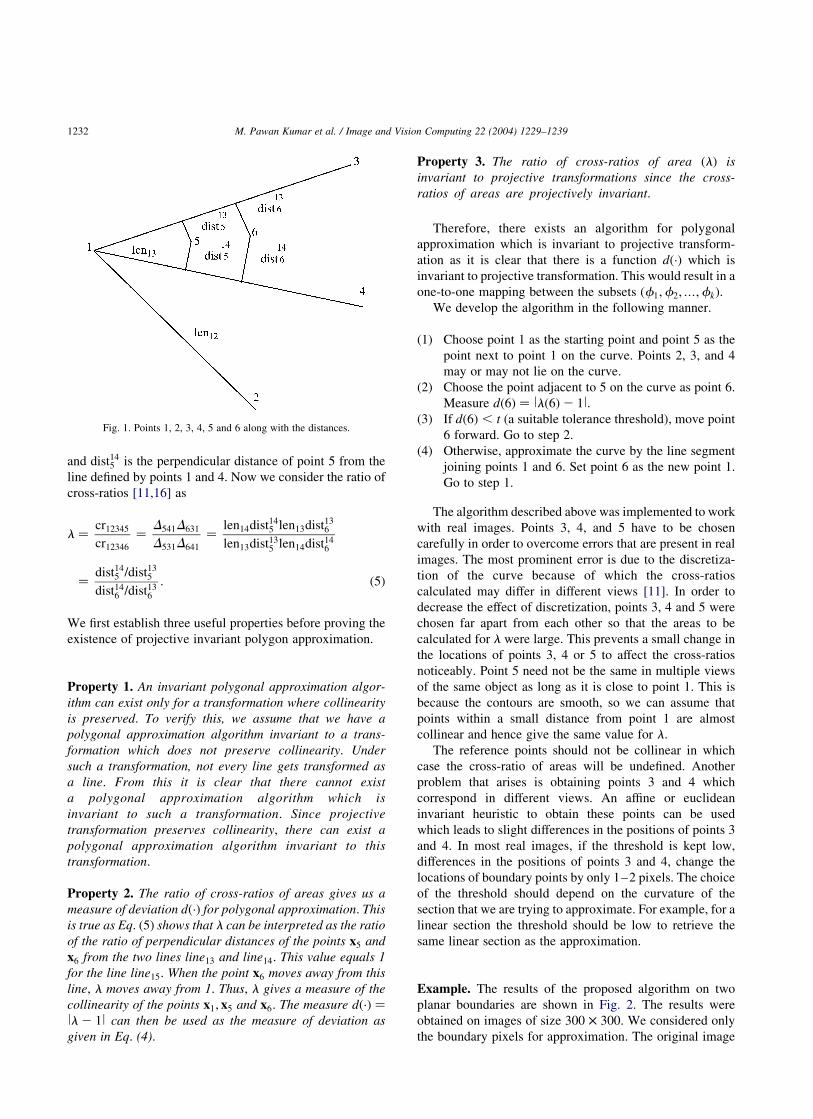
Example. The results of the proposed algorithm on two

planar boundaries are shown in Fig. 2. The results were

obtained on images of size 300 £ 300. We considered only

the boundary pixels for approximation. The original image

Fig. 1. Points 1, 2, 3, 4, 5 and 6 along with the distances.


is shown on top with two projectively transformed versions

below it. The boundary pixels are drawn in black colour.

The red lines in the figure show the polygonal approxi-

mation of the boundary using our algorithm. The green lines

show the projectively transformed polygon which approxi-

mates the original images. The green and red polygons in

the figures are identical in all cases except one or two

breakpoints which got shifted by 1–2 pixels due to

discretization. We obtained good results on other planar

boundaries as well.

3.3. Projectively invariant piecewise conic approximation

The general method for parametric approximation

described in Section 3.2 can be applied for finding piecewise

conic approximations to a closed curve which is invariant to

projective transformations.Suchamethod ispossiblebecause

a projective invariant exists which can give the measure of

deviation fromaconic section.This invariant is thecross-ratio

of lines which is defined for four concurrent lines as

cr Linesðl1; l2; l3; l4Þ ¼sin u13 sin u24

sin u23 sin u14

ð6Þ

where uij is the angle between lines li and lj: This is invariant

to general linear or projective transformations [11].

This can alternatively be defined for five points in general

position as

crðx1; x2; x3; x4; x5Þ ¼ cr Linesðl15; l25; l35; l45Þ ð7Þ

where lij is the line joining points xi and xj:

According to Chasles’ theorem [23], if we keep x1; x2; x3

and x4 fixed, the locus of all points x such that crðx1; x2;

x3; x4; xÞ is fixed, is a conic curve. If we define l ¼ crðx1;

x2; x3; x4; x5Þ; then the value lcrðx1; x2; x3; x4; xÞ2 ll gives

the measure of separation of point x from the conic defined

by points x1 –x5:

The above results are used to develop an algorithm for

projectively invariant piecewise conic approximation. The

algorithm is similar to the one described for polygonal

approximation except that the measure of deviation used is

the cross-ratio of lines. We denote the starting point by x1:

Points x2; x3; x4 and x5 are chosen near x1 on the curve. We

then move clockwise from point x5 and compute the

deviation dðxÞ as the difference between the cross-ratio of

lines of points ðx1; x2; x3; x4; x5Þ and ðx1; x2; x3; x4; xÞ for

every boundary point x: As long as dðxÞ is less than a suitable

tolerance threshold, the visited points can be approximated

with a conic section. When dðxÞ becomes larger than the

threshold, we put a breakpoint there and continue with the

next point on the boundary as x1:

The algorithm will partition the curve points into sets

which can be approximated using a conic section. A

projectively invariant conic fitting algorithm should then be

used to estimate the conic section which fits those points.

This, however, does not pose a big problem as the points to

be fitted are not highly scattered and therefore algorithms

which are affine or similarity invariant lead to only very

small errors in fitting [22].

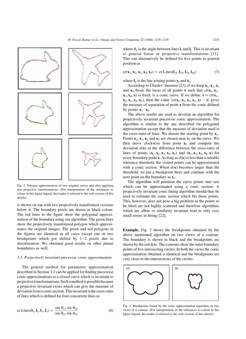
Example. Fig. 3 shows the breakpoints obtained by the

above mentioned algorithm on two views of a contour.

The boundary is shown in black and the breakpoints are

shown by the red dots. The contours show the outer boundary

points of five intersecting circles. In both the views the conic

approximation obtained is identical and the breakpoints are

very close to the intersections of the circles.

Fig. 2. Polygon approximation of two original curves and after applying

two projective transformations. (For interpretation of the references to

colour in this figure legend, the reader is referred to the web version of this

article).

Fig. 3. Breakpoints found by the conic approximation algorithm on two

views of a contour. (For interpretation of the references to colour in this

figure legend, the reader is referred to the web version of this article).


4. Fourier domain affine invariant for discrete contours

In this section, we analyze the properties of a collection

of points, such as a planar object’s contour, in a transform

domain. Collections of points such as a boundary have more

information than isolated points. The sequencing inherent in

such a collection makes a transform domain approach, such

as the Fourier one, a good tool to study their properties. The

linear image-to-image relationships combined with the

properties of the contour in the Fourier domain enable

rich constraints that essentially characterize the contour

independent of the viewpoint. We come up with a view-

independent characterization of the planar shape boundary

using a measure computed in the Fourier domain. Some

preliminary results were presented in Refs. [15,24].

4.1. Fourier domain representation of the contour

Let the Fourier domain representation of the sequence

xl½i�; 0 # i , N (introduced in Section 2) be Xl½k�; 0 # k ,

N such that

Xl½k� ¼

Ul½k�

Vl½k�

Wl½k�

26664

37775

where Ul½k�; Vl½k�; and Wl½k� are, respectively, the Fourier

transforms of the individual sequences ul½i�; vl½i�; and wl½i�:

We call this the vector Fourier representation of the contour.

Note that the sequences Xl½k� are periodic and conjugate

symmetric.

Theorem 1. The Fourier transform and the collineation

commute with the above representation. That is, if points are

transformed between views 0 and l using Eq. (1), the same

homography will transform corresponding frequency terms

in the Fourier domain also. In other words

Xl½k� ¼ MlX0½k�; 0 # k , N: ð8Þ

Proof. Let Ml ¼ mlij; 1 # i; j # 3: Expanding Eq. (1) for the

u term

ul½i� ¼ ml11u0½i� þ ml

12v0½i� þ ml13w0½i�

Taking the Fourier transform of the above equation and

using the linearity property of Fourier transforms, we get

Ul½k� ¼ ml11U0½k� þ ml

12V0½k� þ ml13W0½k�

Similarly for Vl½k� and Wl½k� (note that wl½i� need not be 1).

It is now easy to see that

Xl½k� ¼ MlX0½k�

giving us the desired result. A

Given a set of M views, the recognition problem can be

formulated as the identification of a view-independent

function f ð·Þ such that f ðx0; x1;…; xMÞ ¼ 0: This recognition

constraint can be linear or nonlinear in image coordinates.

The algebraic relation given by f ð·Þ can then be used to settle

the question whether the M observed views were of the

same object.

4.2. Rank constraint for recognition

If the image-to-image homography is affine, the

transformation matrix has ml31 ¼ ml

32 ¼ 0 and ml33 ¼ 1:

The transformation can be expressed in terms of inhomo-

geneous coordinates as

xl½i� ¼ Alx0½i� þ bl ð9Þ

where xl½i� is the inhomogeneous representation of the ith

pointon thecontour inview l;Al is theupper2 £ 2minorofMl

and bl is the upper two elements of the last column of Ml:

The above expression is valid for the scenarios when

correspondence between points across views is known.

However, in practice, correspondence is rarely available. In

case correspondence information is not available, Eq. (9)

assumes the form

xl½i� ¼ Alx0½i þ ll� þ bl

where cyclic shifting of the sequence x0 by ll would align

the corresponding points of x0 and xl: The frequency

domain representation can be given by

Xl½k� ¼ AlX0½k�expj2pllk

N

� ; 0 , k , N ð10Þ

if the bl term is eliminated by omitting the k ¼ 0 term in the

Fourier domain.

Let us define a measure called the cross-conjugate

product on the Fourier representations of two views as

cð0; lÞ½k� ¼ ðX0½k�ÞpTXl½k�;

0 , k , N ¼ ðX0½k�ÞpTAlX0½k�expj2pllk

N

� :

ð11Þ

The matrix Al can be expressed as a sum of a symmetric

matrix and a skew symmetric matrix as Al ¼ Als þ Al

sk

where Als ¼

12ðAl þ ðAlÞTÞ and Al

sk ¼ 12ðAl 2 ðAlÞTÞ:

The skew symmetric matrix reduces to

c0 1

21 0

" #;

where c ¼ ml12 2 ml

21 is the difference of the off-diagonal

elements of Al: We now have

cð0; lÞ½k� ¼ X0½k�pTðAls þ Al

skÞX0½k�exp

j2pllk

N

�

The term X0½k�pTAlsX

0½k� is purely real while the term

X0½k�pTAlskX0½k� is purely imaginary. We observe that


the effect of the transformation matrix Al on the second term

is restricted to a scaling by a factor c: We can define a new

measure k; ignoring scale, for the sequence Xl in view l as

kðlÞ½k� ¼ Xl½k�pT0 1

21 0

" #Xl½k�: ð12Þ

It can be shown (see Appendix A) that

kðlÞ½k� ¼ lAllkð0Þ½k�; 0 , k , N ð13Þ

where lAll is the determinant of A: Eq. (13) gives a

necessary condition for the sequences X0 and Xl to be two

affine views of the same planar shape, or in other words, the

values of the measure kð·Þ in the two views should be scaled

versions of each other. The kð·Þ values for a contour are,

thus, signatures of that contour. This extends to multiple

views also. Consider the MðN 2 1Þ matrix formed by the

coefficients of the kð·Þ measures for M different views

Q ¼

kð0Þ½1� · · · kð0Þ½N 2 1�

kð1Þ½1� · · · kð1Þ½N 2 1�

· · · · · · · · ·

kðM 2 1Þ½1� · · · kðM 2 1Þ½N 2 1�

26666664

37777775

The necessary condition for matching of the planar shape in

M views then reduces to

rankðQÞ ¼ 1: ð14Þ

The view independent function that we want is f ð·Þ ¼ 0 ;rankðQÞ2 1 ¼ 0: It should be noted that this recognition

constraint does not require correspondence across views and

is valid for any number of views.

Since, the k measures in the various views are only

scaled versions of each other, if we normalize the k measure

terms in each view with respect to a fixed one then

gðlÞ½k� ¼ kðlÞ½k�=kðlÞ½p�; p is fixed

¼ ðlAllkð0Þ½k�Þ=ðlAllkð0Þ½p�Þ ¼ kð0Þ½k�=kð0Þ½p�

gðlÞ½k� ¼ gð0Þ½k� ð15Þ

The terms of the normalized k measure—the g measure are

independent of the view. Hence, g is an affine view invariant

of a contour, whose computation does not need correspon-

dence information across views.

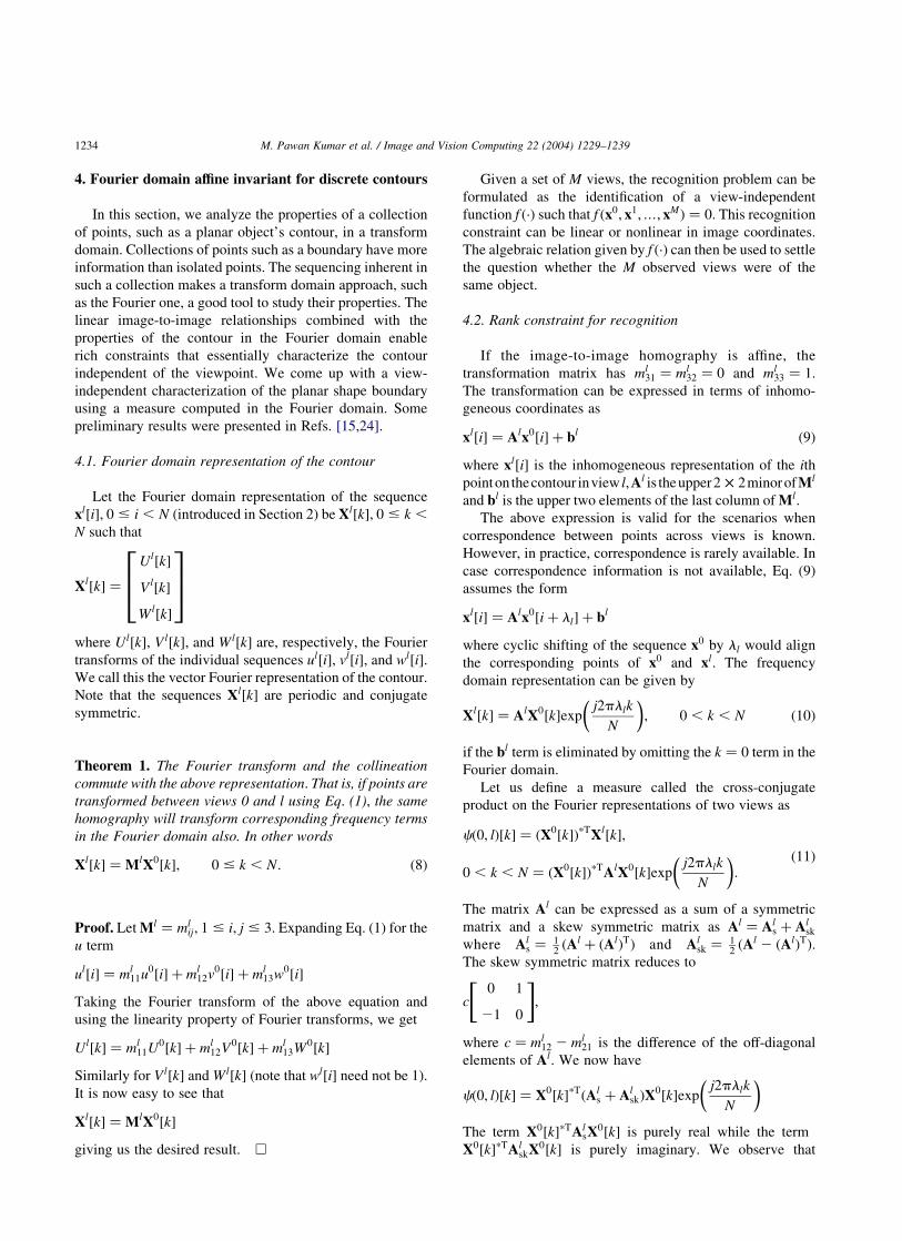
Example. We consider four views of a dinosaur shown in

Fig. 4. These views are related by affine transformations.

Euclidean measures are not preserved under these trans-

formations. However, we can still recognize them using the

rank constraint. Discretization noise does introduce errors

into the framework that make the rank constraint an

approximation, but the constraint is robust and still works

appreciably. To verify whether a matrix has rank r; we

consider the ratio of rth to ðr þ 1Þth singular values of

the matrix. This ratio is high if the matrix has rank r: To

determine whether the rank of Q is 1, we need to compare

the ratio of the highest two singular values. The ratios of two

highest singular values of Q constructed from various two-

view combinations of views shown in Fig. 4 are arranged in

Table 1.

5. Polygons in multiple views

The recognition mechanism developed in Section 4 can

be used for recognizing polygons under affine image-to-

image homographies. In this section, we formulate a

technique for recognizing polygons in multiple views,

specifically when the optical axes of the cameras used for

imaging are coincident. We represent the boundary as a

sequence of lines instead of points. This is applicable when

the objects are polygons or the representation is an

approximation.

When a planar object is being imaged from multiple view

points so that attention is focused on it, the location of the

view points can be characterized using the azimuthal angle a

in the horizontal plane, the elevation angleb from the vertical

axis, the twist angle t about its own axis, and the distance d

from the origin (Fig. 5(a)). The image-to-image homography

H12 relating two views given by ða1;b1; t1; d1Þ and

ða2;b2; t2; d2Þ due to the object plane can be expressed up

Fig. 4. Four affine transformed views of a dinosaur.

Table 1

Ratio of the highest singular value to the second highest singular value of Q

constructed from various two-view combinations of views shown in Fig. 4

Dinosaur 1 Dinosaur 2 Dinosaur 3 Dinosaur 4

Dinosaur 1 – 43,176.5 23,988.5 35,453.9

Dinosaur 2 43,176.5 – 25,733.7 35,352.6

Dinosaur 3 23,988.5 25,733.7 – 17,548

Dinosaur 4 35,453.9 35,352.6 17,548 –


to scale as

H ¼

d1r2

11 r121

r212 r1

22

�� 2d1

r211 r1

11

r212 r1

12

�� 0

d1r2

21 r121

r222 r1

22

�� 2d1

r221 r1

11

r222 r1

12

�� 0

A B C

266666666664

377777777775

where

A ¼r1

21 ðd1r231 2 d2r1

31Þ

r122 ðd1r2

32 2 d2r132Þ

��; B ¼

r111 ðd1r2

31 2 d2r131Þ

r112 ðd1r2

32 2 d2r132Þ

��;

C ¼ d2r1

11 r112

r121 r1

22

��

and r1ij and r2

ij are the entries of the 3 £ 3 rotation matrices that

relate the vertical view to the view given by ðai;bi; tiÞ;

respectively, for the views 1 and 2. This homography matrix

has the special form of the transpose of an affine homography.

If the homography H relates points in two views, then H2T

relates corresponding lines in two views. Therefore, if the

homography relating corresponding points in two views has

the form of transpose of affine, corresponding lines in the two

views are related by affine image-to-image homographies.

So, if we represent the boundary in a line space—making use

of the edges of the polygons we can use the same approach as

outlined in Section 4.2 for achieving recognition.

Example. Fig. 5(b) shows two views of a polygon, whose

vertices are related by a homography whose transpose has

the form of an affine homography. Hence, corresponding

edges are related by affine homographies. All lines were

normalized, so that the third component of each line was

unity. The Q matrix was computed from the line

representation of the polygon. Its rank was essentially 1 as

its highest singular values was 11,061.5 times bigger than

the next highest singular value.

6. Applications and extensions

6.1. Numeral recognition

We demonstrate the applicability of polygonal approxi-

mation and the Fourier domain invariant to recognition of

numerals. Numeral recognition has been conventionally

addressed among the document image processing commu-

nity. Popular OCRs are designed to address this problem

only under similarity transformations. There are many other

situations in image and video processing where the

numerals are to be recognized under transformations more

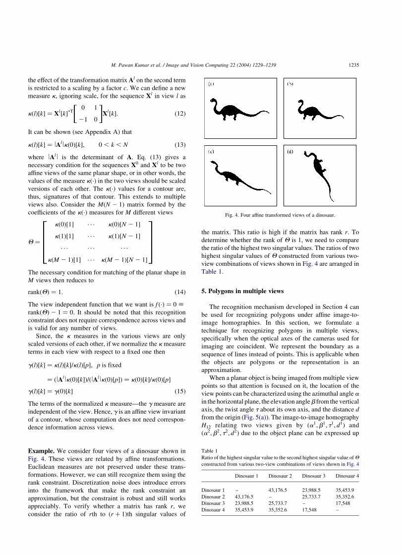
general than similarity. For instance, the alpha numerals on

a number plate imaged from different viewpoints undergo

projective transformations as can be seen in Fig. 6(a). We

tried approximating the numerals in multiple views.

Fig. 6(b) shows the result of approximating the numeral 8

in the two views shown in Fig. 6(a).

The numerals in the multiple views are related by

projective homographies. Though the Fourier domain

invariant has been derived for affine image-to-image

homographies, we empirically found it to be applicable to

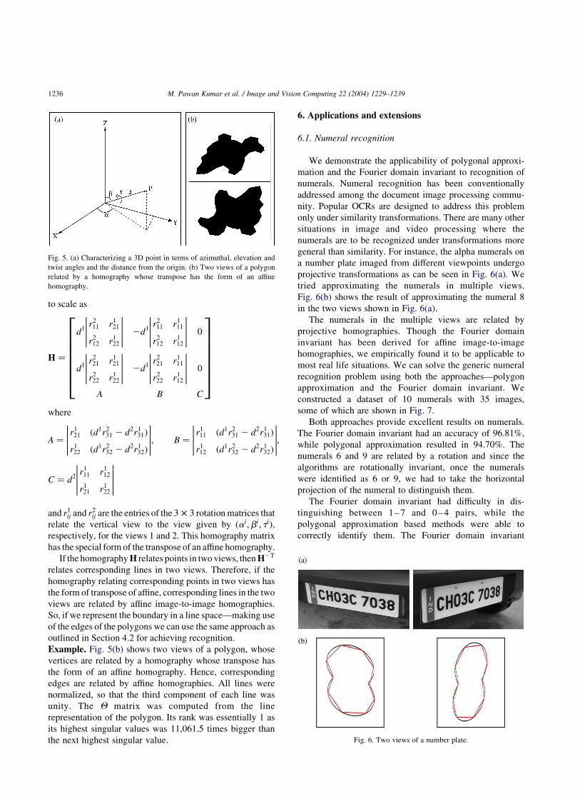
most real life situations. We can solve the generic numeral

recognition problem using both the approaches—polygon

approximation and the Fourier domain invariant. We

constructed a dataset of 10 numerals with 35 images,

some of which are shown in Fig. 7.

Both approaches provide excellent results on numerals.

The Fourier domain invariant had an accuracy of 96.81%,

while polygonal approximation resulted in 94.70%. The

numerals 6 and 9 are related by a rotation and since the

algorithms are rotationally invariant, once the numerals

were identified as 6 or 9, we had to take the horizontal

projection of the numeral to distinguish them.

The Fourier domain invariant had difficulty in dis-

tinguishing between 1 – 7 and 0 – 4 pairs, while the

polygonal approximation based methods were able to

correctly identify them. The Fourier domain invariant

Fig. 5. (a) Characterizing a 3D point in terms of azimuthal, elevation and

twist angles and the distance from the origin. (b) Two views of a polygon

related by a homography whose transpose has the form of an affine

homography.

Fig. 6. Two views of a number plate.


works well when the boundary has more detail (presence of

high frequencies). Thus, the problem in distinguishing 1 and

7 is to be expected.

6.2. Aircraft recognition

Most aircrafts can be recognized from their boundaries.

Hence, shape based approaches for their recognition have

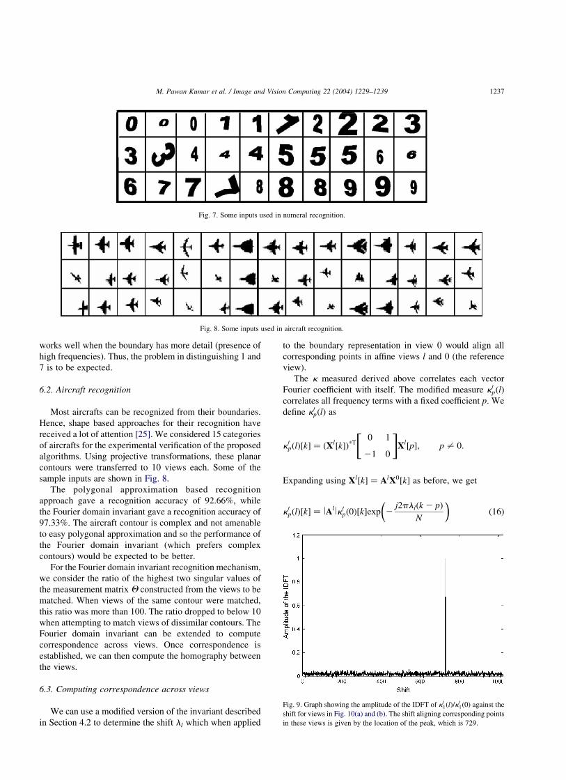
received a lot of attention [25]. We considered 15 categories

of aircrafts for the experimental verification of the proposed

algorithms. Using projective transformations, these planar

contours were transferred to 10 views each. Some of the

sample inputs are shown in Fig. 8.

The polygonal approximation based recognition

approach gave a recognition accuracy of 92.66%, while

the Fourier domain invariant gave a recognition accuracy of

97.33%. The aircraft contour is complex and not amenable

to easy polygonal approximation and so the performance of

the Fourier domain invariant (which prefers complex

contours) would be expected to be better.

For the Fourier domain invariant recognition mechanism,

we consider the ratio of the highest two singular values of

the measurement matrix Q constructed from the views to be

matched. When views of the same contour were matched,

this ratio was more than 100. The ratio dropped to below 10

when attempting to match views of dissimilar contours. The

Fourier domain invariant can be extended to compute

correspondence across views. Once correspondence is

established, we can then compute the homography between

the views.

6.3. Computing correspondence across views

We can use a modified version of the invariant described

in Section 4.2 to determine the shift ll which when applied

to the boundary representation in view 0 would align all

corresponding points in affine views l and 0 (the reference

view).

The k measured derived above correlates each vector

Fourier coefficient with itself. The modified measure k0pðlÞ

correlates all frequency terms with a fixed coefficient p: We

define k0pðlÞ as

k0pðlÞ½k� ¼ ðXl½k�ÞpT0 1

21 0

" #Xl½p�; p – 0:

Expanding using Xl½k� ¼ AlX0½k� as before, we get

k0pðlÞ½k� ¼ lAllk0pð0Þ½k�exp 2j2pllðk 2 pÞ

N

� ð16Þ

Fig. 7. Some inputs used in numeral recognition.

Fig. 8. Some inputs used in aircraft recognition.

Fig. 9. Graph showing the amplitude of the IDFT of k01ðlÞ=k01ð0Þ against the

shift for views in Fig. 10(a) and (b). The shift aligning corresponding points

in these views is given by the location of the peak, which is 729.


and

k0pðlÞ½k�

k0pð0Þ½k�¼ lAllexp 2

j2pllðk 2 pÞ

N

� ð17Þ

Eq. 17 states that the quotient series k0pðlÞ=k0pð0Þ would be a

complex sinusoid, whose inverse Fourier transform would

show a distinct peak at the shift that would align

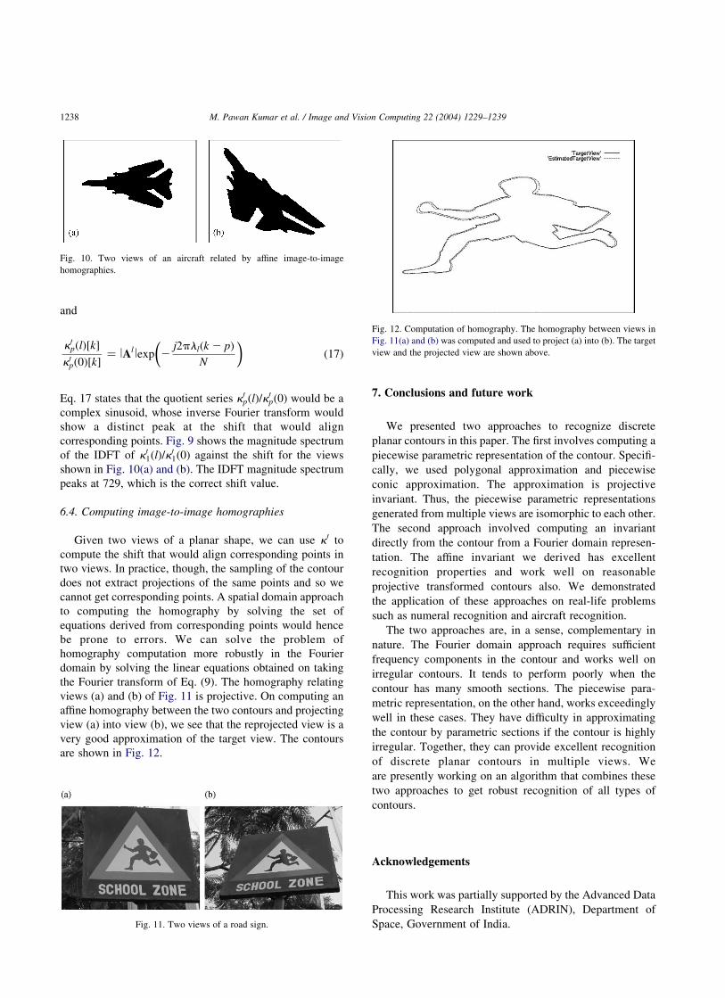
corresponding points. Fig. 9 shows the magnitude spectrum

of the IDFT of k01ðlÞ=k01ð0Þ against the shift for the views

shown in Fig. 10(a) and (b). The IDFT magnitude spectrum

peaks at 729, which is the correct shift value.

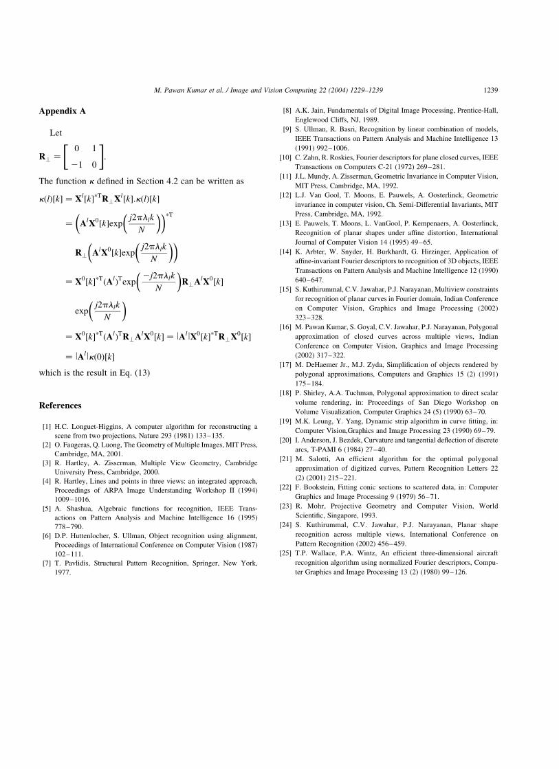
6.4. Computing image-to-image homographies

Given two views of a planar shape, we can use k0 to

compute the shift that would align corresponding points in

two views. In practice, though, the sampling of the contour

does not extract projections of the same points and so we

cannot get corresponding points. A spatial domain approach

to computing the homography by solving the set of

equations derived from corresponding points would hence

be prone to errors. We can solve the problem of

homography computation more robustly in the Fourier

domain by solving the linear equations obtained on taking

the Fourier transform of Eq. (9). The homography relating

views (a) and (b) of Fig. 11 is projective. On computing an

affine homography between the two contours and projecting

view (a) into view (b), we see that the reprojected view is a

very good approximation of the target view. The contours

are shown in Fig. 12.

7. Conclusions and future work

We presented two approaches to recognize discrete

planar contours in this paper. The first involves computing a

piecewise parametric representation of the contour. Specifi-

cally, we used polygonal approximation and piecewise

conic approximation. The approximation is projective

invariant. Thus, the piecewise parametric representations

generated from multiple views are isomorphic to each other.

The second approach involved computing an invariant

directly from the contour from a Fourier domain represen-

tation. The affine invariant we derived has excellent

recognition properties and work well on reasonable

projective transformed contours also. We demonstrated

the application of these approaches on real-life problems

such as numeral recognition and aircraft recognition.

The two approaches are, in a sense, complementary in

nature. The Fourier domain approach requires sufficient

frequency components in the contour and works well on

irregular contours. It tends to perform poorly when the

contour has many smooth sections. The piecewise para-

metric representation, on the other hand, works exceedingly

well in these cases. They have difficulty in approximating

the contour by parametric sections if the contour is highly

irregular. Together, they can provide excellent recognition

of discrete planar contours in multiple views. We

are presently working on an algorithm that combines these

two approaches to get robust recognition of all types of

contours.

Acknowledgements

This work was partially supported by the Advanced Data

Processing Research Institute (ADRIN), Department of

Space, Government of India.

Fig. 10. Two views of an aircraft related by affine image-to-image

homographies.

Fig. 12. Computation of homography. The homography between views in

Fig. 11(a) and (b) was computed and used to project (a) into (b). The target

view and the projected view are shown above.

Fig. 11. Two views of a road sign.


Appendix A

Let

R’ ¼0 1

21 0

" #:

The function k defined in Section 4.2 can be written as

kðlÞ½k� ¼ Xl½k�pTR’Xl½k�:kðlÞ½k�

¼ AlX0½k�expj2pllk

N

� � pT

R’ AlX0½k�expj2pllk

N

� �

¼ X0½k�pTðAlÞTexp2j2pllk

N

� R’AlX0½k�

expj2pllk

N

�

¼ X0½k�pTðAlÞTR’AlX0½k� ¼ lAllX0½k�pTR’X0½k�

¼ lAllkð0Þ½k�

which is the result in Eq. (13)

References

[1] H.C. Longuet-Higgins, A computer algorithm for reconstructing a

scene from two projections, Nature 293 (1981) 133–135.

[2] O. Faugeras, Q. Luong, The Geometry of Multiple Images, MIT Press,

Cambridge, MA, 2001.

[3] R. Hartley, A. Zisserman, Multiple View Geometry, Cambridge

University Press, Cambridge, 2000.

[4] R. Hartley, Lines and points in three views: an integrated approach,

Proceedings of ARPA Image Understanding Workshop II (1994)

1009–1016.

[5] A. Shashua, Algebraic functions for recognition, IEEE Trans-

actions on Pattern Analysis and Machine Intelligence 16 (1995)

778–790.

[6] D.P. Huttenlocher, S. Ullman, Object recognition using alignment,

Proceedings of International Conference on Computer Vision (1987)

102–111.

[7] T. Pavlidis, Structural Pattern Recognition, Springer, New York,

1977.

[8] A.K. Jain, Fundamentals of Digital Image Processing, Prentice-Hall,

Englewood Cliffs, NJ, 1989.

[9] S. Ullman, R. Basri, Recognition by linear combination of models,

IEEE Transactions on Pattern Analysis and Machine Intelligence 13

(1991) 992–1006.

[10] C. Zahn, R. Roskies, Fourier descriptors for plane closed curves, IEEE

Transactions on Computers C-21 (1972) 269–281.

[11] J.L. Mundy, A. Zisserman, Geometric Invariance in Computer Vision,

MIT Press, Cambridge, MA, 1992.

[12] L.J. Van Gool, T. Moons, E. Pauwels, A. Oosterlinck, Geometric

invariance in computer vision, Ch. Semi-Differential Invariants, MIT

Press, Cambridge, MA, 1992.

[13] E. Pauwels, T. Moons, L. VanGool, P. Kempenaers, A. Oosterlinck,

Recognition of planar shapes under affine distortion, International

Journal of Computer Vision 14 (1995) 49–65.

[14] K. Arbter, W. Snyder, H. Burkhardt, G. Hirzinger, Application of

affine-invariant Fourier descriptors to recognition of 3D objects, IEEE

Transactions on Pattern Analysis and Machine Intelligence 12 (1990)

640–647.

[15] S. Kuthirummal, C.V. Jawahar, P.J. Narayanan, Multiview constraints

for recognition of planar curves in Fourier domain, Indian Conference

on Computer Vision, Graphics and Image Processing (2002)

323–328.

[16] M. Pawan Kumar, S. Goyal, C.V. Jawahar, P.J. Narayanan, Polygonal

approximation of closed curves across multiple views, Indian

Conference on Computer Vision, Graphics and Image Processing

(2002) 317–322.

[17] M. DeHaemer Jr., M.J. Zyda, Simplification of objects rendered by

polygonal approximations, Computers and Graphics 15 (2) (1991)

175–184.

[18] P. Shirley, A.A. Tuchman, Polygonal approximation to direct scalar

volume rendering, in: Proceedings of San Diego Workshop on

Volume Visualization, Computer Graphics 24 (5) (1990) 63–70.

[19] M.K. Leung, Y. Yang, Dynamic strip algorithm in curve fitting, in:

Computer Vision,Graphics and Image Processing 23 (1990) 69–79.

[20] I. Anderson, J. Bezdek, Curvature and tangential deflection of discrete

arcs, T-PAMI 6 (1984) 27–40.

[21] M. Salotti, An efficient algorithm for the optimal polygonal

approximation of digitized curves, Pattern Recognition Letters 22

(2) (2001) 215–221.

[22] F. Bookstein, Fitting conic sections to scattered data, in: Computer

Graphics and Image Processing 9 (1979) 56–71.

[23] R. Mohr, Projective Geometry and Computer Vision, World

Scientific, Singapore, 1993.

[24] S. Kuthirummal, C.V. Jawahar, P.J. Narayanan, Planar shape

recognition across multiple views, International Conference on

Pattern Recognition (2002) 456–459.

[25] T.P. Wallace, P.A. Wintz, An efficient three-dimensional aircraft

recognition algorithm using normalized Fourier descriptors, Compu-

ter Graphics and Image Processing 13 (2) (1980) 99–126.


Documents

Discrete contours in multiple views: approximation and recognition