Discriminative Semi-parametric Trajectory

Model for Speech Recognition

K. C. Sim and M. J. F. Gales

Cambridge University Engineering Department,

Trumpington Street, Cambridge,

CB2 1PZ United Kingdom

Abstract

Hidden Markov Models (HMMs) are the most commonly used acoustic model forspeech recognition. In HMMs, the probability of successive observations is assumedindependent given the state sequence. This is known as the conditional indepen-

dence assumption. Consequently, the temporal (inter-frame) correlations are poorlymodelled. This limitation may be reduced by incorporating some form of trajectorymodelling. In this paper, a general perspective on trajectory modelling is provided,where time varying model parameters are used for the Gaussian components. A dis-criminative semi-parametric trajectory model is then described where the Gaussianmean vector and covariance matrix parameters vary with time. The time variation ismodelled as a semi-parametric function of the observation sequence via a set of cen-troids in the acoustic space. The model parameters are estimated discriminativelyusing the Minimum Phone Error (MPE) criterion. The performance of these mod-els is investigated and benchmarked against a state-of-the-art CUHTK Mandarinevaluation systems.

Key words: speech recognition, trajectory model, discriminative training,minimum phone error

1 Introduction

Hidden Markov Models (HMMs) [18] are widely used as the acoustic modelin speech recognition. A series of assumptions underlie the use of HMMs tomodel the speech data, some of which are poor. In particular, the “conditionalindependence assumption” implies that the observation output probability is

Email address: [kcs23,mjfg]@eng.cam.ac.uk (K. C. Sim and M. J. F. Gales).

Preprint submitted to Elsevier Science 23 March 2007

conditionally independent of all other observations given the current state.This yields a constant trajectory within an HMM state. Existing ways to over-come this limitation include the use of switching linear dynamical system [19],stochastic segment model [13, 12], polynomial segment model, buried Markovmodel [2] and trajectory HMM [21, 22]. In general, all these models are collec-tively known as trajectory models. To date, maximum likelihood training ofthese models has had very little success in large vocabulary continuous speechrecognition. In this paper, a discriminative semi-parametric trajectory modelwill be presented. This model represents the Gaussian mean vectors and covari-ance matrices as time varying parameters. These time dependent parametersare modelled as a function of the location of the current observation (and theneighbouring observations) in the acoustic space, which is represented by aseries of centroids. Model parameters are discriminatively estimated using theMinimum Phone Error (MPE) [17] criterion.

One form of temporally varying mean vector is obtained by applying a timedependent bias to the static Gaussian mean. This time dependent bias isa weighted contribution from the bias vectors associated with each centroid(to be estimated discriminatively). The contribution weights are calculatedas the posteriors of the centroids given the observation (and neighbouringobservations). The resulting model yields an fMPE model [16, 15]. This wasoriginally presented as a feature transformation, but may also be describedin the semi-parametric trajectory framework described here. The variance ofeach dimension may also be scaled by a positive time dependent factor to yielda temporally varying covariance matrix. This model will be referenced to aspMPE [20]. Similar to fMPE, the time dependent scale factor is a weightedcontribution from the centroid specific scales where the weights are given bythe posteriors of the observations given the centroids. Both of these models andtheir combination may be described as a semi-parametric trajectory model.

This paper is organised as follows. Section 2 introduces several forms of trajec-tory models applied to speech recognition and establishes a general formulationof time varying model parameters for trajectory models. This formulation isthen used to introduce a semi-parametric trajectory model in Section 3. Next,Section 4 derives the parameter estimation formulae of this form of modelusing the Minimum Phone Error (MPE) criterion. Section 4.4 discusses theimplementation issues. In Section 6, experimental results are given based ona large vocabulary conversational telephone speech recognition task. Finally,conclusions are given in Section 7.

2

2 Trajectory Models

There are a number of modelling approaches that have attempted to over-come the HMM conditional independence assumption. These include the useof switching linear dynamical systems [19], stochastic segment models [13,12], polynomial segment models, buried Markov models [2] and trajectoryHMM [21, 22]. All these models have a common aim of relaxing the “condi-tional independence assumption” by allowing the state output distribution tovary with time. This time variation is achieved by adding dependency on theobservation sequence, OT

1 , either directly or indirectly using latent variables.The model parameters for the state output probability are now viewed as timedependent such that

p(OT1 |Q

T1 , θt) =

T∏

t=1

p(ot|θt) (1)

where the time dependent parameter set, θt, is expressed as a function of theobservation sequence, OT

1 , state sequence, QT1 , and the time, t, i.e.

θt = f(

OT1 , QT

1 , t; θ)

(2)

The form of function, f(.), with parameters, θ, defines the type of model used.As with standard HMMs, it is convenient to represent the output densityfunction as a Gaussian Mixture Model (GMM) [8] as it can be used to modelany arbitrary non-Gaussian distribution and its model parameters may beestimated efficiently. In this case, the GMM parameters are time dependent:

p(ot|θt) =M∑

m=1

csmtN (ot; µsmt,Σsmt) (3)

where θt = {csmt, µsmt,Σsmt}. These time varying Gaussian parameters maybe expressed as a general function of the form given in equation (2). Therefore,

{csmt, µsmt,Σsmt} = f(

OT1 , QT

1 , t; θc, θµ, θΣ

)

(4)

where θc, θµ and θΣ denote the model parameters for the component weight,mean and covariance matrix respectively.

In the following sections, several trajectory and segmental models will be de-scribed within the time varying parameter formulation given by equations (1)and (2).

3

2.1 Explicit Temporal Correlation Modelling

One of the earliest work on explicit time correlation modelling was carried outby Wellekens [23] where correlations between adjacent frames are explicitlymodelled. This yields a time varying mean of the following form:

µst = µs + ΣsuΣ−1uu (ot−1 − µu) (5)

where s and u denote the current and previous states. µs and Σss are the meanvector and covariance matrix respectively of state s. Σsu is the cross covariancematrix between state s and u. This is a special form of equation (4) whereθµ = {µs, µu,Σss,Σuu,Σsu}.

Vector linear prediction (VLP) is also a trajectory model [24], where the stateoutput probability of ot is conditionally independent of other parameters giventhe current state, qt, and observation dependencies, Ht. The resulting meanvector becomes time dependent of the form

µst = µ(0)s +

P∑

p=1

A(p)s

(

ot+τp− µ(τp)

s

)

(6)

where P is the number of predictors. The mean vector given the HMM stateis dependent on the observation history, Ht = {ot+τp

: 1 ≤ p ≤ P, 1 ≤ t+ τp ≤T}. This form of model is again a specific form of a time varying parameterformulation given by equation (4) with θµ = {µ(0)

s , A(p)s , µ(τp)

s }.

2.2 Implicit Temporal Correlation Modelling

Another type of trajectory modelling approach is to model the temporal cor-relations implicitly via some form of latent structures. An example of thisapproach is the Buried Markov Model (BMM) [2]. This model defines an ad-ditional latent variable, buried under the hidden states of HMMs. This latentvariable defines the class of dependencies of emitting an observation, ot, attime t. In [2], a Gaussian-mixture BMM was described where the state outputdensity function is modelled by a mixture of Gaussian of the form

p(ot|ht, qt = s, θ)=M∑

m=1

V∑

v=1

P (m|s, v)P (v|ht)N (ot; µsmvt,Σsmv)

=M∑

m=1

V∑

v=1

csmvtN (ot; µsmvt,Σsmv) (7)

4

where ht is a column vector defining the entire collection of dependencies vari-ables any element of ot might use and v denotes the class of ht. M and V arethe number of components and classes respectively. P (m|s, v), the prior ofcomponent m, given the state s and class v, is a discrete probability table andP (v|ht) is the probability of class v given the continuous vector ht. This for-mulation yields a time varying Gaussian mean vector and component weight,given by

µsmvt =Asmvht + bsmv (8)

csmvt =P (m|s, v)p(v|ht) (9)

where Asmv, bsmv and P (m|s, v) are model parameters that can be estimatedefficiently using the EM approach [2]. These expressions are dependent on timevia the vector of dependency variables, ht. The term Asmvht may be viewedas a time varying bias applied to bsmv, the mean of component m, given thestate s and class v.

The Switching Linear Dynamical System (SLDS) [19] also belongs to the tra-jectory model family. The generative model of an SLDS is given by the fol-lowing state-space formulation

xt = Asxt−1 + ws

ot = Csxt + vs

where

ws ∼ N(

ws; µ(x)s ,Σ(x)

s

)

vs ∼ N(

vs; µ(o)s ,Σ(o)

s

)(10)

where s denotes the discrete state generated by the underlying Markov chainwithin the HMM. As and Cs are state dependent linear transformation ma-trices while ws and vs are random vectors whose mean vectors and covariancematrices are also dependent on s. Therefore, the mean of observation givenby this model is of the following time varying form

µst = Cs

(

Asxt−1 + µ(x)s

)

+ µ(o)s (11)

The time varying property arises due to the dependency on the continuouslatent state variable, xt−1. The trajectory is modelled implicitly by the stateevolution process. Note, the latent state variable, xt, can be expressed as afunction of As and xt0 , where t0 is the time of entering state s, by applyingthe first expression in equation (10) recursively. Thus, the trajectory within astate depends on the initial latent state when entering that state. This initiallatent state is a function of the previous states visited and the durations spentin those states. The trajectory is therefore an implicit function of the historicalstate sequence.

Up to this point, a generic formulation of time varying parameters has been

5

used to describe various existing trajectory models. In the following section,a semi-parametric trajectory model is introduced using the same formulation.

3 Semi-parametric Trajectory Model

The form of semi-parametric trajectory model considered in this paper can beformulated by expressing the mean vector and precision matrix as follows:

µsmt = Atµsm + bt (12)

P smt = ZtP smZt′ (13)

where At and Zt are the time dependent linear transformations for the meanvector, µsm, and precision matrix, P sm, respectively. Precision matrix is de-fined as the inverse of the covariance matrix (P sm = Σ−1

sm). bt denotes atime dependent bias vector for the mean. The form of time dependent lin-ear transformations and bias considered in this work will be described laterin Section 3.1. When the linear transformations are set as identity matrices(At = Zt = I) and the bias vector is set as a zero vector (bt = 0), the aboveexpressions degenerate to the mean and precision matrix of a standard HMMsystem. The form of trajectory model described by equations 12 and 13 canbe viewed as applying a time varying affine transformation to the componentmean vectors and precision matrices in the system. An important question ishow to determine the appropriate form of time varying transformations. Inthis section a semi-parametric representation will be described.

It is worth pointing out that using a full transformation matrices for equa-tions (12) and (13) is impractical in many situations due to the high com-putational cost in applying the transformation at each time to each Gaussiancomponent in the system (typical LVCSR systems comprise more than 100,000Gaussian components). This problem may be alleviated by using diagonaltransforms. Transformations can then be applied independently per dimen-sion. Equations (12) and (13) may then be expressed as scaling and shiftingof the mean and diagonal precision matrix elements for each dimension:

µsmtj = atjjµsmj + btj (14)

psmtj = z2tjjpsmj (15)

where µsmtj and btj are the jth element of µsmt and bt respectively. psmtj , andztjj denote the jth diagonal element of P smt, and Zt respectively and At isassumed to be a diagonal matrix. µsmj and psmj denote the jth element of thetime independent mean and precision matrix respectively for component m instate s. In this work, only diagonal covariance matrix systems are considered,

6

with the additional constraint that At is an identity matrix. In Section 4,the semi-parametric trajectory model parameters estimation will be presentedbased on the use of an identity matrix for the mean transformation, At anda diagonal transform for the precision matrix, Zt. The latter transformationwill be referred to as the pMPE model.

3.1 A Semi-parametric Representation

Modelling of the time variation in the linear transformation is an importantaspect for these trajectory models. A semi-parametric representation will beconsidered here. First, a series of centroids is defined to represent the regionsof interest in the acoustic feature space. Associated with the ith centroid, thefollowing parameters are defined:

• A(i): a linear transformation matrix for the mean vector• Z(i): a linear transformation matrix for the precision matrix• b(i): a bias vector for the mean vector

The corresponding time varying affine transformations discussed above will bemodelled as a weighted contribution from all the centroids:

At = I +n∑

i=1

hi(t)A(i) (16)

bt =n∑

i=1

hi(t)b(i) (17)

Zt = I +n∑

i=1

hi(t)Z(i) (18)

where hi(t) denotes the contribution weights from the i centroid at time t

and n is the total number of centroids. The resulting time varying mean biashas a similar form to that of a Buried Markov Model (Asmvht), as shown inequation (8). To be more precise, hi(t) is equivalent to the ith element of ht

and b(i) is the ith column of Asmv. The two methods differ by the way ht

is defined. Nonetheless, ht is used to capture the temporal variation in themodel parameters in both cases.

Each centroid is modelled using a Gaussian component. Let gi denote the ithcentroid represented by the Gaussian component N (ot; µi,Σi) such that thelikelihood of gi given a d-dimensional observation, ot, is given by

p(ot|gi) =1

√

(2π)d|Σi|exp

{

−1

2(ot − µi)

′Σ−1

i (ot − µi)}

(19)

7

The weights, hi(t) is then computed as the posterior probability of gi givenot,

hi(t) = P (gi|ot) =p(ot|gi)P (gi)

∑nj=1 p(ot|gj)P (gj)

(20)

where P (gi), the prior probability of gi, is assumed to be uniformly distributedin this work. Consider a two-dimensional example in Figure 1. The centroids

o

g1

P (g1|ot)

g2

P (g2|ot)

g3

P (g3|ot)

g4

P (g4|ot)

g5

P (g5|ot)

g6

P (g6|ot)

g7

P (g7|ot)

g8

P (g8|ot) Centroid

Observation

Fig. 1. Obtaining interpolation weights from the posterior of a set of centroids giventhe observation sequence

may be considered as a Vector-Quantisation (VQ) codebook representing theacoustic space. The posterior probabilities, P (gi|ot), would then be the proba-bilistic quantisation of ot. Thus, the interpolation formulae given in equations(16), (17) and (18) can be viewed as the weighted contribution from the trans-formations associated with each centroid given the position of the observationin the acoustic space. This formulation is analogous to the way the outputprobabilities are computed for semi-continuous HMMs, which leads to theinterpretation of the above trajectory model as a semi-parametric model.

Figure 2 depicts the visualisation of the semi-parametric trajectory model us-ing a two-dimensional example. The interpolation weights are computed as aprobabilistic VQ feature at each time t (see Figure 1) which tracks the ob-servation as a smoothed trajectory. Interpolation using these time-dependentweights yields a trajectory of the Gaussian parameters, µsmt and Σsmt, con-ditioned upon the observation sequence, as given by equations (12) and (13)respectively.

8

t=1 t=2 t=3 t=T

(µsm1,Σsm1) (µsm2,Σsm2) (µsm3,Σsm3) (µsm4,Σsm4)

Fig. 2. A semi-parametric representation of the Gaussian parameters

3.2 Context Expansion for Semi-parametric Trajectory Model

In the semi-parametric trajectory model formulation, context expansion can beviewed as increasing the modelling power of the trajectory. All the discussionsso far have been considering only the observation vector at the current time, t.It is possible to extend the dependency to a window of observations around t

to allow for context expansion. Equations (16), (17) and (18) may be expressedin a more generic form as follows:

At = I +C∑

τ=−C

w(τ)n∑

i=1

hi(t + τ)A(i)τ (21)

bt =C∑

τ=−C

w(τ)n∑

i=1

hi(t + τ)b(i)τ (22)

Zt = I +C∑

τ=−C

w(τ)n∑

i=1

hi(t + τ)Z(i)τ (23)

where w(τ) is the window function of length 2C +1, i.e. considering C frameson either side of the current frame. C can be viewed as the context of thetrajectory. The window function used in this work follows the same as thatintroduced in [16], where

w(τ) =

1 τ = 0

12

τ = ±1,±2...

1N

τ = ±N(N−1)2

,±(

N(N−1)2

+ 1)

, . . . , C

(24)

9

and

C =

(

N(N − 1)

2+ N − 1

)

(25)

When a window function that spans a large number of frames is used, it isnecessary to tie the dynamic parameters to prevent over-training issue. Thiswork adopts the same window length and tying scheme introduced in [16]. Inthat paper, a window length of 19 frames (N = 4, C = 9) was used. Withoutparameter tying, the number of dynamic parameters will be 19 times morethan those without context expansion. To reduce the total number of freeparameters, the dynamic parameters are tied across frames {1,2}, {3,4,5} and{6,7,8,9} to the left and right of the current frame, according to the partitionsshown in equation (24). From the definitions of w(τ) in equation (24), this isequivalent to taking the average posteriors within the partitions so that thetrue expansion in terms of the dynamic parameters is only ±3 (7 times morethan that without context expansion).

Though, it appears as if context expansion is essential to modelling trajectorysince it takes into consideration neighbouring observation, this is not the case.The key element of this semi-parametric trajectory model lies in the fact thatthe position of the acoustic vector at each time is tracked in a semi-parametric

way by using a set of centroids representing the acoustic space. Thus trajectoryinformation is maintained by the observation vector itself. Context expansionsimply extends the modelling power of the trajectory model by also consideringthe position of the neighbouring observation vectors. This allows the shortterm movement of the observation vectors to be captured, at the expense ofincreased model parameters.

4 Parameter Estimation

The parameterisation of the semi-parametric trajectory model can be broadlydivided into those associated with the standard HMMs (θh) and those asso-ciated with the centroids (θc). In the rest of this discussion, θh and θc willbe referred to as the static and dynamic parameters respectively to empha-sise that the latter capture the temporally varying attributes of the trajectorymodel. This section derives the estimation formulae for these parameters usingthe MPE criterion [17]. The MPE objective function is a measure of the ex-pected phone accuracy of recognising the training data given the HMM model.This is given by

Rmpe(θ) =U∑

u=1

∑

w∈Wu

P (w|OT1 , θ)PhoneAcc(w, w) (26)

10

where θ encompasses both θh and θc. PhoneAcc(w, w) denotes the measureof phone accuracies of hypothesis w given the reference w and Wu is the setof competing hypotheses for sentence u. U is the total number of sentencesin the training set. It is difficult to directly maximise this objective functiondirectly. Instead, a weak-sense auxiliary function [17] is used. The weak-senseauxiliary function to be optimised is given by

Qmpe(θ, θ) =T∑

t=1

S∑

s=1

M∑

m=1

γmpesm (t) log p(ot|θ) (27)

where the log likelihood of component m in state s is given by,

log p(ot|θ) = Ksm −1

2

d∑

j=1

{

log(σ2smtj) +

(otj − µsmtj)2

σ2smtj

}

(28)

Ksm subsumes all terms that are independent of the model parameters. T

is the total number of training speech frames, M is the number of Gaussiancomponents per state and S is the total number of states in the system.γmpe

sm (t) is a quantity computed for MPE training [14], which can be regardedas the ‘MPE posterior’ of component m in state s at time t. This quantity iscomputed as the difference between the numerator and denominator posteriorsof component m in state s at time t (γn

sm(t) and γdsm(t) respectively). Typically,

these posteriors are also smoothed by using the D-smoothing and I-smoothingtechniques to obtain improved performance.

Maximising the above weak-sense auxiliary function with respect to all themodel parameters (θh and θc) is not trivial. Hence, these two sets of modelparameters will be updated separately, each time keeping the other parameterset constant.

4.1 Static Parameters Estimation

First, consider the update of the static parameters given that the dynamic pa-rameters are held constant. The weak-sense auxiliary function in equation (27)may be rewritten in terms of the trajectory model parameters as

Qmpe(θ, θ) = K −1

2

S∑

s=1

M∑

m=1

T∑

t=1

d∑

j=1

γmpesm (t)

{

log(σ2smtj) +

(otj − µsmtj)2

σ2smtj

}

(29)

where K subsumes all the constant terms. The new parameters are found suchthat the differential of the auxiliary function with respect to the parametersat the new estimates equals to zero. Thus,

11

∂Qmpe(θ, θ)

∂µsmj

=T∑

t=1

(

∂Qmpe(θ, θ)

∂µsmtj

∂µsmtj

∂µsmj

)

=T∑

t=1

γmpesm (t)

(otj − µsmtj)

σ2smtj

= 0 (30)

∂Qmpe(θ, θ)

∂σ2smj

=T∑

t=1

(

∂Qmpe(θ, θ)

∂σ2smtj

∂σ2smtj

∂σ2smj

)

=1

2

T∑

t=1

γmpesm (t)

σ2smtj − (otj − µsmtj)

2

(σ2smtj)

2

z2tjj = 0 (31)

Solving the above equations yields the update formulae for the jth element ofthe mean and variance as

µsmj =xmpe

smj

βmpe

smj

and σ2smj =

wmpe

smj

βmpesm

(32)

where the sufficient statistics are given by

βmpesm =

T∑

t=1

γmpesm (t) (33)

βmpe

smj =T∑

t=1

γmpesm (t)z2tjj (34)

xmpe

smj =T∑

t=1

γmpesm (t)z2tjj

(

otj − btj

)

(35)

wmpe

smj =T∑

t=1

γmpesm (t)z2tjj

(

otj − btj − µsmj

)2(36)

Note that βmpesm is already accumulated in the standard HMM parameters up-

date for MPE training. xmpe

smj and wmpe

smj are the jth element of the mean andcovariance matrix statistics given by equation (44), with the exception thatthe component posterior is scaled by z2tjj and the observation is shifted by btj

for each dimension j. The additional statistics required is the d-dimensionalβmpe

smj .

4.2 Dynamic Parameters Estimation

Having estimated the static parameters, the dynamic parameters may be es-timated by keeping the static parameters constant. Here, the update of thecentroid specific bias, b

(i)j , and scaling factor, z

(i)j , for the jth element of the

mean vector and precision matrix will be described. Due to the large number

12

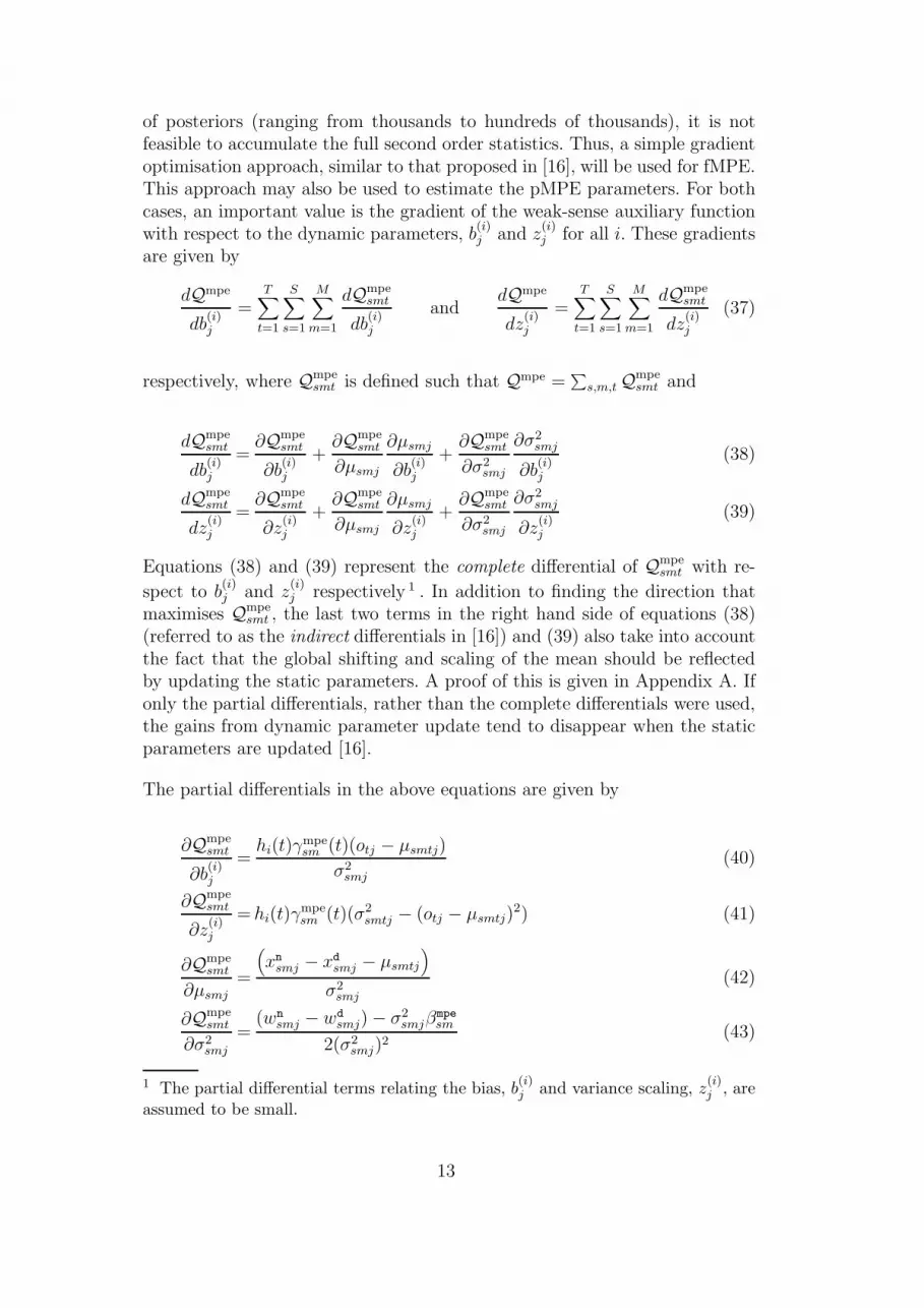
of posteriors (ranging from thousands to hundreds of thousands), it is notfeasible to accumulate the full second order statistics. Thus, a simple gradientoptimisation approach, similar to that proposed in [16], will be used for fMPE.This approach may also be used to estimate the pMPE parameters. For bothcases, an important value is the gradient of the weak-sense auxiliary functionwith respect to the dynamic parameters, b

(i)j and z

(i)j for all i. These gradients

are given by

dQmpe

db(i)j

=T∑

t=1

S∑

s=1

M∑

m=1

dQmpesmt

db(i)j

anddQmpe

dz(i)j

=T∑

t=1

S∑

s=1

M∑

m=1

dQmpesmt

dz(i)j

(37)

respectively, where Qmpesmt is defined such that Qmpe =

∑

s,m,t Qmpesmt and

dQmpesmt

db(i)j

=∂Qmpe

smt

∂b(i)j

+∂Qmpe

smt

∂µsmj

∂µsmj

∂b(i)j

+∂Qmpe

smt

∂σ2smj

∂σ2smj

∂b(i)j

(38)

dQmpesmt

dz(i)j

=∂Qmpe

smt

∂z(i)j

+∂Qmpe

smt

∂µsmj

∂µsmj

∂z(i)j

+∂Qmpe

smt

∂σ2smj

∂σ2smj

∂z(i)j

(39)

Equations (38) and (39) represent the complete differential of Qmpesmt with re-

spect to b(i)j and z

(i)j respectively 1 . In addition to finding the direction that

maximises Qmpesmt , the last two terms in the right hand side of equations (38)

(referred to as the indirect differentials in [16]) and (39) also take into accountthe fact that the global shifting and scaling of the mean should be reflectedby updating the static parameters. A proof of this is given in Appendix A. Ifonly the partial differentials, rather than the complete differentials were used,the gains from dynamic parameter update tend to disappear when the staticparameters are updated [16].

The partial differentials in the above equations are given by

∂Qmpesmt

∂b(i)j

=hi(t)γ

mpesm (t)(otj − µsmtj)

σ2smj

(40)

∂Qmpesmt

∂z(i)j

= hi(t)γmpesm (t)(σ2

smtj − (otj − µsmtj)2) (41)

∂Qmpesmt

∂µsmj

=

(

xnsmj − xd

smj − µsmtj

)

σ2smj

(42)

∂Qmpesmt

∂σ2smj

=(wn

smj − wdsmj) − σ2

smjβmpesm

2(σ2smj)

2(43)

1 The partial differential terms relating the bias, b(i)j and variance scaling, z

(i)j , are

assumed to be small.

13

where xnsmj and wn

smj are the jth element of the MPE sufficient numeratorstatistics xn

sm and W nsm respectively. These sufficient statistics are given by

xnsm =

T∑

t=1

γmlsm(t)ot and W n

sm =T∑

t=1

γmlsm(t) (ot − µsm) (ot − µsm)′ (44)

The denominator statistics, xdsmj and wd

smj, are defined in a similar fashion.

The forms of the remaining differentials ∂µsmj

∂b(i)j

,∂σ2

smj

∂b(i)j

, ∂µsmj

∂z(i)j

and∂σ2

smj

∂z(i)j

depend

on the update methods for the static parameters, µsmj and σ2smj . Ideally, MPE

updates of all the parameters, including the static parameters, is preferred.However, the use of the D-smoothing and the I-smoothing with dynamicML (or dynamic MMI) priors in standard MPE training [17] complicates thecalculation of the indirect differentials. The next section describes a simplerform of update that yields efficient robust parameter estimation.

4.3 Interleaved Dynamic-Static Parameters Estimation

Simultaneous updates of both the static and dynamic parameters does notyield a closed form solution. A standard approach to this problem is to adoptan interleaved procedure where the static and the dynamic parameters arealternately updated. This allows the use of the gradients defined in the Sec-tions 4.1 and 4.2. However it is still necessary to obtain the partial differentialsof, for example,

∂µsmj

∂b(i)j

. To simplify this, and avoiding the issues of D-smoothing

and I-smoothing, ML updates of the static parameters are considered whenestimating the dynamic parameters. This makes the partial differentials simpleto specify. After the dynamic parameters have been estimated, discriminative(MPE) training of the static parameters is then performed. This approach issimilar to that proposed by Povey et al. in [16] and will be described in moredetail below.

The interleaved parameter estimation procedure is summarised as follows:

1. Start from an ML trained model

2. Estimate dynamic parameters using MPE criterion

3. Estimate static parameters using ML criterion

4. When sufficient iterations performed, go to step 6

5. Go to step 2

6. Estimate static parameters using MPE criterion

Figure 3: The interleaved dynamic static parameter estimation procedure

14

It may seem strange to interleave updates with two different objective func-tions. However, provided that the appropriate static parameter update formu-lae are used in the complete differentials, the resulting dynamic parameterswill capture the temporally varying aspect of the parameters. These completedifferentials are crucial to prevent oscillation when interleaving between twodifferent criteria [16].

The ML estimates of the static parameters are found by keeping the dynamicparameters constant, as described in Section 4.1, but using ML, rather thanMPE, posteriors. The dynamic model parameters can then be estimated usingthe gradient in equations (38) and (39). As the static parameters are foundusing the ML criterion in the subsequent training iteration, the partial dif-ferential of the mean and variance with respect to the dynamic parametersare evaluated by differentiating equations in (32) with respect to b

(i)j and z

(i)j ,

which yields

∂µsmj

∂b(i)j

=−hi(t)γ

mlsm(t)

βmlsmj

(45)

∂σ2smj

∂b(i)j

=−2hi(t)ztjjγ

mlsm(t)(otj − µsmtj)

βmlsm

(46)

∂µsmj

∂z(i)j

=2ztjjγ

mlsm(t)(otj − µsmtj)

βmlsmj

hi(t) −z2tjjγ

mlsm(t)

βmlsmj

(47)

∂σ2smj

∂z(i)j

=2hi(t)ztjjγ

mlsm(t)(otj − µsmtj)

2

βmlsm

(48)

When ztjj = 1, equations (45) and (46) become those of the standard fMPEpresented in [16]. Once the gradient information is computed, the dynamicparameters are updated as follows:

b(i)j = b

(i)j + η

(i)j

dQmpe

db(i)j

and z(i)j = z

(i)j + ν

(i)j

dQmpe

dz(i)j

(49)

where b(i)j and z

(i)j denote the updated parameters for b

(i)j and z

(i)j respectively.

η(i)j and ν

(i)j are the element specific learning rate for b

(i)j and z

(i)j which are

defined as

η(i)j =

ασj

φ(b)ij + ρ

(b)ij

and ν(i)j =

α

φ(z)ij + ρ

(z)ij

(50)

respectively. α is a scalar parameter for adjusting the learning rate and σj is

the average standard deviation of the Gaussian components in the system. φ(b)ij

15

and ρ(b)ij are the sum of the positive and negative contributions to the gradient

of Qmpesmt with respect to b

(i)j at each time, t, as presented in [16]. A similar

approach may be used for φ(z)ij and ρ

(z)ij , which determine the learning rate for

the precision scaling. Hence,

φ(b)ij =

T∑

t=1

max

S∑

s=1

M∑

m=1

dQmpe

db(i)j

, 0

and ρ(b)ij =

T∑

t=1

max

−S∑

s=1

M∑

m=1

dQmpe

db(i)j

, 0

φ(z)ij =

T∑

t=1

max

S∑

s=1

M∑

m=1

dQmpe

dz(i)j

, 0

and ρ(z)ij =

T∑

t=1

max

−S∑

s=1

M∑

m=1

dQmpe

dz(i)j

, 0

After updating the dynamic parameters (and the static parameters using ML),the static parameters may be updated using MPE training. This is achievedusing the original update equations in (32).

It is possible to stop the training process after performing dynamic parameters,without any additional MPE training of the static parameters. In this paperto denote the difference, where only the dynamic parameters are updated thiswill be denoted as, for example, pMPE. Where additional MPE training of thestatic parameters has been performed this will be referred to as pMPE+MPE.

4.4 Implementation Issues

First, the likelihood computation of fMPE and pMPE models will be exam-ined. As fMPE may be implemented as a feature transformation, the additionalcost for the likelihood calculation of fMPE model is negligible compared to thestandard HMM system 2 . For pMPE there is a slight increase in this cost. Thelikelihood of the model parameters, θ = {µsmj , σ

2smj}, given the observation

vector, ot, is given by

log p(ot|θ) = K +1

2

d∑

j=1

{

log ztjj − log σ2smj −

ztjj(otj − µsmj)2

σ2smj

}

(51)

This requires an extra d multiplications and 1 addition compared to the stan-dard model. It also requires ztjj and

∑dj=1 log ztjj to be cached for each frame.

2 The additional cost is due to the computation of the posterior probabilities forthe centroids, which can be achieved efficiently by using some kind of Gaussianselection techniques [16]

16

pMPE parameter estimation was found to be less robust than fMPE and wasmore likely to be overtrained. This is not surprising as second order statis-tics are used. To handle this problem, the values of α for precision scalingestimation were typically set to be less than those for MPE (α < 1.0). Fur-thermore, in some cases the temporally varying scale, z2tjj tended a value closeto zero. This was felt to be due to the wrap-around from squaring ztjj. Forexample, if ztjj is close to zero, its value may oscillate and change sign overtime. However, squaring ztjj ignores the sign and may result in an undesirablewrap-around effect to the trajectory of the precision scale factor. To preventthis, a minimum value is applied to ztjj, similar to the concept of varianceflooring:

ztjj = max{ztjj, zmin} (52)

where ztjj is the floored scale factor and zmin is the scale floor. In this work,zmin has been set to 0.1.

5 Relationship to Linear Adaptation and fMPE

The general form of semi-parametric trajectory modelling given in equations (12)and (13) resembles that of linear transformation based speaker and environ-ment adaptation, for example Maximum Likelihood Linear Regression (MLLR)adaptation formulae for mean vector [10] and covariance matrix [6] respec-tively. The semi-parametric formulation of equations (12) and (13) may beviewed as a time-varying linear adaptation of model parameters, dependingon the position and movement of the observation vector in the acoustic space.

Instead of applying time varying transforms to the Gaussian parameters, theymay also be applied to the feature vectors.

ot = Ctot + dt (53)

where ot and ot are the original and transformed observation vectors. Thisis equivalent to setting the case where the linear transformation matrices forthe mean vector and covariance matrices are the same. This is analogousto viewing Constrained MLLR [4] as a restrictive form of MLLR mean andvariance adaptations.

It is interesting to note that equation (53) is identical to the fMPE model [16]when Ct = I. In this case, a time varying bias, dt, is applied to the features.This is equivalent to subtracting the same bias from the mean vectors (dt =

17

−bt). In [16], the time varying feature offset is given by

dt = Mht (54)

where M is a projection matrix from the high dimensional vector of posteriors(ht = [h1(t) h2(t) . . . hn(t)]′) to standard feature size. Comparing this toequation (17), it is clear that the columns of M are given by −b(i).

6 Experimental Results

The experimental results presented in this section are based on a Conver-sational Telephone Speech Mandarin (CTS-M) task. All the systems in theseexperiments used 12 Perceptual Linear Prediction (PLP) coefficients [7] withthe C0 energy term and the first three derivatives. Heteroscedastic Linear Dis-criminant Analysis (HLDA) [9] was then applied to project the feature downto 39 dimensions. Pitch and its first two derivatives were appended to thisfeature vector to yield a 42-dimensional feature-space. Finally, Gaussianisa-tion [5] was applied to normalise the features per conversation side. For moredetails of the system configuration, see [5].

The acoustic models were trained using 72 hours of ldc04 and swm03 dataprovided by LDC. Decision tree state-clustered triphones were used. All thesystems used in this work had approximately 4000 distinct states. System eval-uation was performed on two test sets: dev04 (2 hours) and eval04 (1 hour).

For the semi-parametric trajectory models, 4000 centroids were used to ob-tain the time varying mean offset and precision scaling. These centroids wereobtained from the baseline system with 4000 distinct states and one Gaussiancomponent per states. This is considerably smaller than that used in fMPE [16](approximately 100,000 centroids). Preliminary experiments showed that us-ing more centroids (obtained, for example, from the Gaussian components ofa 16-component per state ML system) leads to over-training problem due tolimited available training data. For each observation, most of the posteriorvalues were very small (close to zero). Gaussian clustering and minimum pos-terior threshold were used as a simple Gaussian selection process to improvethe computational efficiency. It was empirically found that Gaussian compo-nents with high posterior values are almost always found wihtin the 5 nearestgroup. Furthermore, it was found that centroids with posterior value below0.1 do not contribute very much to the trajectory modelling. These valueswere used in all the experiments in this paper. Without context expansion,there were on average about two non-zero posteriors per frame. The numberof nonzero posteriors increases to 14 per frame when a ±3 context expansionwas used.

18

6.1 Single Component Systems

The first set of experiments were conducted on a simple single-component-per-state systems. This allows semi-parametric trajectory modelling to be ex-amined without the effect of implicit trajectory modelling due to the use ofmultiple components. The baseline system was obtained by performing eightMPE iterations, starting from an ML trained system. From the same MLsystem, the fMPE and pMPE systems were trained with 4 iterations usingthe interleaved update (see Section 4.3). These systems were furthered refinedwith 8 MPE iterations to yield the fMPE+MPE and pMPE+MPE systems.

Figure 4 shows the improvement in the MPE criterion with increasing trainingiterations for various single component systems. The top and bottom graphscorrespond to systems without and with ±3 context expansions respectively.The initial dotted lines indicate fMPE/pMPE training and the final solid linesdenote the 8 iterations of standard MPE training. The MPE criterion for thebaseline MPE system increases from 0.49 to 0.59. Without context expansion,the fMPE and pMPE models yielded a much lower absolute MPE criteriongain of 0.023 and 0.011 respectively after 4 iterations. However, with additionaleight MPE training iterations, the criterion obtained were slightly better thanthe baseline (approximately 0.60).

The modelling power of the systems greatly improved when a ±3 contextexpansion was used. This is clearly reflected from the criterion gain shown inthe figure. From the same figure, the variation is the MPE criterion for thepMPE system with ±3 context expansion follows closely to that of the MPEsystem. Furthermore, the gain from fMPE with context expansion is clearlybetter than the baseline. The final systems, fMPE+MPE and pMPE+MPE,were about 0.05 and 0.03 better in terms of MPE criterion.

Systemdev04 eval04

0 ±3 0 ±3

MPE 44.4 42.2

fMPE+MPE 42.1 40.1 39.4 37.3

pMPE+MPE 43.3 41.3 40.4 38.6

fMPE+pMPE+MPE 41.6 38.9 39.2 36.6

Table 1CER performance of 1-component fMPE and pMPE systems with 0 and ±3 contextexpansion on dev04 and eval04 for CTS-M task

The Character Error Rate (CER) performance of the above systems on dev04

and eval04 is summarised in Table 1. The baseline single component MPEalone system gave 44.4% and 42.2% CER on dev04 and eval04 respectively.

19

0 2 4 6 8 10 12

0.5

0.52

0.54

0.56

0.58

0.6

Plot of MPE criterion against number of training iterations

Number of iterations

MP

E C

riter

ion

MPEfMPEfMPE+MPEpMPEpMPE+MPEfMPE+pMPEfMPE+pMPE+MPE

0 2 4 6 8 10 12

0.5

0.55

0.6

0.65

Plot of MPE criterion against number of training iterations

Number of iterations

MP

E C

riter

ion

MPEfMPEfMPE+MPEpMPEpMPE+MPEfMPE+pMPEfMPE+pMPE+MPE

Fig. 4. Change in MPE criterion with increasing training iterations for single com-ponent systems without context expansion (top) and with ±3 context expansion(bottom)

20

The fMPE+MPE system improved the baseline by 2.3–2.8% without con-text expansion. In the same configuration, pMPE+MPE system, gave smallergains, absolute improvements of 1.1–1.8%. In combination, fMPE+pMPE+MPE,additional gains of 0.2–0.5% over the fMPE+MPE system were obtained.

If context expansion of ±3 was used both fMPE and pMPE showed gainsover the no context expansion cases. For the pMPE+MPE system absoluteimprovements of 3.1–3.6% were obtained over the baseline MPE system. How-ever, again the gains from pMPE+MPE were smaller than those using fMPE+MPE.Combining the two approaches together gave total gains of about 5.5% abso-lute over the baseline MPE system.

Several important conjectures can be made based on these results. First, whena simple acoustic model was used, the gains obtained from the fMPE andpMPE techniques became significantly larger. The loss in the modelling powerof the static parameters has been compensated by the dynamic parameters.Moreover, the pMPE+MPE system combined well with context expansion.This provides a clear indication that the pMPE+MPE with ±3 context ex-pansion suffered from an over-fitting problem. In addition, promising gainswere also obtained by combining the fMPE and pMPE techniques to yield thefMPE+pMPE+MPE system.

As previously mentioned, the fMPE and pMPE techniques may be viewed asa semi-parametric trajectory model. From this perspective, the single com-ponent fMPE and pMPE systems also provided an interesting account forthe trajectory modelling aspects of the system. Because the systems underconsideration have only one Gaussian component per state, the observationsassociated with each state in a standard HMM are independent and iden-tically distributed (i.i.d.) with a normal distribution. Thus, the trajectorywithin each HMM state is piece-wise constant. By incorporating the fMPEand pMPE techniques to the single component systems, promising improve-ments as shown in Table 1 were obtained.

Figures 5 and 6 show the trajectory of the fMPE+MPE and pMPE+MPEmodels. Note that the standard MPE system models the observation sequencewith a piece-wise linear trajectory. Both the fMPE+MPE and pMPE+MPEsystems were capable of model more flexible trajectories. Because the modelparameters were estimated using discriminative training, the resulting trajec-tories may not follow that of the observation. The actual time varying meanoffset and precision scale are depicted in the bottom graphs of Figures 5 and6 respectively. The mean offset has a range between -0.2 to 0.3 while theprecision scale falls between 0.7 to 1.6.

21

50 100 150 200 250 300

−2

−1

0

1

2

Frame

PLP

Coe

ffici

ent 1

Trajectory for fMPE+MPE model

observationMPE trajectoryfMPE+MPE trajectory

50 100 150 200 250 300−0.2

−0.1

0

0.1

0.2

Frame

Mea

n of

fset

Mean offset for fMPE+MPE model

Fig. 5. Top: fMPE+MPE trajectory compared with the MPE trajectory and thecorresponding observation for the first dimension of the feature; Bottom: Timevarying mean offset for fMPE

50 100 150 200 250 300−3

−2

−1

0

1

2

Frame

PLP

Coe

ffici

ent 1

Trajectory for pMPE+MPE model

observationMPE trajectory±1 Std. Dev. of pMPE trajectory

50 100 150 200 250 300

0.8

1

1.2

1.4

1.6

1.8

Frame

Pre

cisi

on s

cale

Precision Scale for pMPE+MPE model

Fig. 6. Top: MPE trajectory and the corresponding observation for the first dimen-sion of the feature. Shaded area represents the uncertainty of the pMPE trajectorywithin ±1 standard deviation; Bottom: Time varying precision scale for pMPE

22

6.2 Multiple Component Systems

As with the single component systems, the same set of experiments were alsoconducted on 16-component systems to examine the gains from fMPE andpMPE on more complex systems. Table 2 summarises the CER results. The

Systemdev04 eval04

0 ±3 0 ±3

MPE 36.0 33.9

fMPE+MPE 35.6 34.4 33.7 32.5

pMPE+MPE 35.9 35.4 33.7 33.8

fMPE+pMPE+MPE 35.3 34.7 33.5 33.1

Table 2CER performance of 16-component fMPE and pMPE systems with 0 and ±3 contextexpansion on dev04 and eval04 for CTS-M task

CER of the baseline MPE system was 36.0% and 33.9% on dev04 and eval04

respectively. As expected, the gains from the fMPE+MPE and pMPE+MPEsystems were found to be smaller compared to the single component systems.The former yielded gains of 0.2–0.4% without context expansion and 1.4–1.6%with ±3 context expansion. There is a large improvement to the CER per-formance when context information is considered. Unfortunately, apart fromthe 0.6% absolute improvement on dev04, the gains from the pMPE+MPEsystem almost disappeared compared to the gains obtained for the single com-ponent systems. When combining fMPE and pMPE, the 0.2% absolute gainwas obtained on both test sets when without having context expansion. How-ever, a degradation of 0.3–0.6% in performance was observed when ±3 contextexpansion was used. Clearly, the pMPE parameters cannot be reliably esti-mated when used with systems with high complexity. In the next section, analternative approach to combining fMPE and pMPE is pursued.

6.3 Systems Combination

From the above results, it was found that directly combining fMPE andpMPE did not yield good performance for 16-component systems. Anothermethod of combining these techniques is using Confusion Network Combina-tion (CNC) [11]. CNC is performed by first generating a set of hypotheses(in lattices format) for each individual system. These lattices are convertedto sausage nets of word alternatives with confidence scores assigned to eachword (known as confusion networks). Confusion networks from multiple sys-tems are combined and rescored to obtain the word sequence with the highest

23

confidence score.

System dev04 eval04

S1 MPE 35.0 33.4

S2 fMPE+MPE 33.9 32.2

S3 fMPE+pMPE+MPE 34.0 32.6

S1+S2CNC

34.1 32.2

S2+S3 33.3 31.6

Table 3CER performance of confusion network decoding and combination of 16-componentfMPE and pMPE systems with ±3 context expansion on dev04 and eval04 forCTS-M task

Table 3 shows the confusion network (CN) decoding [3] results on dev04 andeval04. Similar to the Viterbi decoding results, the fMPE+MPE system (S2)was found to be about 1.1–1.2% better than the MPE alone system (S1) whilethe fMPE+pMPE+MPE system (S3) was 0.1–0.4% worse than S2. In addi-tion, the effect of 2-way system combination using CNC was examined. Due tothe large performance gap between S1 and S2, the combination performancewas at most the same as the best individual system. However, despite thepoorer performance of S3 compared to S2, a further absolute improvementof 0.6–0.8% was obtained when these two systems are combined. This indi-cates that the errors made by the two system are considerably different. Theresulting trajectory modelled by fMPE and pMPE are also different (see Fig-ures 5 and 6). Therefore, shifting the mean vector and scaling the variancetemporally model different aspects of the trajectory which are complimentary.

7 Conclusions

This paper has introduced a discriminative semi-parametric trajectory model.In this model, the state output probability density function is represented by aGaussian Mixture Model (GMM) where the Gaussian mean vector and the di-agonal covariance matrix varies with time. The time dependency is modelledas a smoothed function of the observation sequence using a basis superpo-sition formulation. Each basis is associated with a centroid representing aposition (or movement) in the acoustic space. The corresponding basis coef-ficients are derived from the posterior of its centroid given the current andpossibly the surrounding observations. Hence, the basis coefficients are timedependent which results in temporally varying model parameters. It was alsoshown that this semi-parametric trajectory model is the same as the fMPEtechnique if only the mean vectors are being modelled. In addition, a novel

24

approach of pMPE was also introduced where the precision matrix elementsare modelled as temporally varying parameters. Both fMPE and pMPE werefound to give gains over the MPE alone system on a conversational telephonespeech Mandarin task. It was also found that combining fMPE and pMPEcould be beneficial in some cases.

Acknowledgements

This work was supported by DARPA grant MDA972-02-1-0013. The thesisdoes not necessarily reflect the position or the policy of the US Governmentand no official endorsement should be inferred.

A Appendix

This section provides the proof that using the complete differentials in equa-tion (37) to update the dynamic parameters, as described in Section 4.2,does not result in global shifting and scaling of the static parameters. This isachieved by showing that the complete differentials are zero when only onecentroid is used. This is because with only one centroid, there is only onecontributing factor and the mean bias and variance scale factors will be thesame for all time frames. Therefore, to prevent global shifting or scaling, thecomplete differentials should be zero yield no update in the dynamic parame-ters.

A.1 Proof of Non-global Shifting for fMPE Update

First, consider the complete differential for fMPE (first part of equation (37)).Using equations (38), (40), (42), (43), (45) and (46), the complete differentialfor fMPE is given by

∑

s,m,t

dQmpesmt

db(i)j

=∑

s,m,t

∂Qmpesmt

∂b(i)j

+∂Qmpe

smt

∂µsmj

∂µsmj

∂b(i)j

+∂Qmpe

smt

∂σ2smj

∂σ2smj

∂b(i)j

=∑

s,m,t

γmpesm (t)(otj − µsmtj)

σ2smj

−

(

xnsmj − xd

smj − µsmtj

)

σ2smj

γmlsm(t)

βmlsmj

=∑

s,m

(

xnsmj − xd

smj − µsmtj

σ2smj

−xn

smj − xdsmj − µsmtj

σ2smj

)

= 0 (A.1)

25

using the fact that

hi(t) = 1,T∑

t−1

γmlsm(t) = βml

smj ,T∑

t−1

γmpesm (t)otj = xn

smj − xdsmj (A.2)

and

∑

s.m.t

∂Qmpesmt

∂σ2smj

∂σ2smj

∂b(i)j

=−∑

s,m,t

(

(wnsmj − wd

smj) − σ2smjβ

mpesm

(σ2smj)

2

)(

ztjjγmlsm(t)(otj − µsmtj)

βmlsm

)

=∑

s,m

(

(wnsmj − wd

smj) − σ2smjβ

mpesm

(σ2smj)

2

)

× 0 (A.3)

The final term simplifies to zero by using the static mean update with themean shifts and variance scale factors initialised to zeros and ones respectively(btj = 0 and ztjj = 1), i.e.

µsmtj = µsmj =

∑Tt=1 γml

sm(t)otj∑T

t=1 γmlsm(t)

=

∑Tt=1 γml

sm(t)otj

βmlsm

(A.4)

The ML statistics used in the above equation correspond to those collectedin the previous iteration to obtain the current estimate of µsmj. Since thecomplete differential for fMPE equals to zero when there is only one centroid,therefore the fMPE update does not yield a global shifting of the static meanvectors.

A.2 Proof of Non-global Scaling for pMPE Update

Similarly, consider the complete differential for pMPE (second part of equa-tion (37)). Using equations (39), (41), (42), (43), (47) and (48), the completedifferential for pMPE is given by

∑

s,m,t

dQmpesmt

dz(i)j

=∑

s,m,t

∂Qmpesmt

∂z(i)j

+∂Qmpe

smt

∂µsmj

∂µsmj

∂z(i)j

+∂Qmpe

smt

∂σ2smj

∂σ2smj

∂z(i)j

=∑

s,m,t

γmpesm (t)(σ2

smj − (otj − µsmtj)2)

σ2smtj

+∑

s,m,t

(

(wnsmj − wd

smj) − σ2smjβ

mpesm

(σ2smj)

2

)(

ztjjγmlsm(t)(otj − µsmtj)

2

βmlsm

)

=∑

s,m

(

βmpesm −

(wnsmj − wd

smj)

σ2smj

+(wn

smj − wdsmj)

σ2smj

− βmpesm

)

= 0 (A.5)

26

using the fact that hi(t) = 1 and that the variance scale factors are initialisedto unity (ztjj = 1), then

σ2smtj = σ2

smj =

∑Tt=1 γml

sm(t)(otj − µsmtj)2

βmlsm

(A.6)

(wnsmj − wd

smj) =T∑

t=1

γmpesm (t)(otj − µsmtj)

2 (A.7)

where the ML statistics in the above equation are again obtained the previousiteration. Therefore, the complete differential for pMPE update does not resultin a global scaling of the variances.

References

[1] L. E. Baum and J. A. Eagon. An inequality with applications to statisticalestimation for probabilistic functions of Markov processes and to a modelfor ecology. Bull. Amer. Math. Soc., 73:360–363, 1967.

[2] J. A. Bilmes. Buried Markov models for speech recognition. In Proc.

IEEE Int. Conf. Acoust., Speech, Signal Process., pages 713–716, 1999.[3] G. Evermann and P. C. Woodland. Posterior probability decoding, confi-

dence estimation and system combination. In Proc. Speech Transcription

Workshop, 2000.[4] M. J. F. Gales. Maximum likelihood linear transformations for HMM-

based speech recognition. Technical Report CUED/F-INFENG/TR291,Cambridge University, 1997. (via anonymous) ftp://svr-www.eng.cam.ac.uk.

[5] M. J. F. Gales, B. Jia, X. Liu, K. C. Sim, P. C. Woodland, and K. Yu.Development of the CUHTK 2004 RT04f mandarin conversational tele-phone speech transcription system. In Proc. IEEE Int. Conf. Acoust.,

Speech, Signal Process., pages 861–864, March 2005.[6] M. J. F. Gales and P. C. Woodland. Mean and variance adaptation

within the MLLR framework. Computer Speech and Languages, 10:249–264, 1996.

[7] H. Hermansky. Perceptual Linear Predictive (PLP) analysis of speech.Journal of the Acoustical Society of America, 87(4):1738–1752, 1990.

[8] B. J. Huang, S. E. Levinson, and M. M. Sondhi. Maximum likelihoodestimation for multivariate mixture observations of Markov chains. IEEE

Trans. Information Theory, IT-32:307–309, March 1986.[9] N. Kumar. Investigation of Silicon-Auditory Models and Generalization

of Linear Discriminant Analysis for Improved Speech Recognition. PhDthesis, Johns Hopkins University, 1997.

[10] C. J. Legetter and P. C. Woodland. Maximum likelihood linear regression

27

speaker adaptation of contiuous density HMMs. Computer Speech and

Languages, 1997.[11] L. Mangu, E. Brill, and A. Stolcke. Finding consensus among words:

Lattice-based word error minimization. In Proc. Eur. Conf. Speech Com-

mun. Technol., 1999.[12] M. Ostendorf, V. Digalakis, and O. Kimball. From HMM’s to segment

models: A unified view of stochastic modeling for speech recognition.IEEE Transactions on Speech and Audio Processing, 4(5):360–378, 1996.

[13] M. Ostendorf and S. Roukos. A stochastic segment model for phoneme-based continuous speech recognition. IEEE Trans on Acoustics, Speech

and Signal Processing, 37(12):1857–1869, 1989.[14] D. Povey. Discriminative Training for Large Vocabulary Speech Recogni-

tion. PhD thesis, Cambridge University, 2003.[15] D. Povey. Improvements to fMPE for discriminative training of features.

In Proc. Interspeech, September 2005.[16] D. Povey, B. Kingsbury, L. Mangu, G. Saon, H. Soltau, and G. Zweig.

fMPE: Discriminatively trained features for speech recognition. In Proc.

IEEE Int. Conf. Acoust., Speech, Signal Process., 2005.[17] D. Povey and P. C. Woodland. Minimum Phone Error and I-smoothing

for improved discriminative training. In Proc. IEEE Int. Conf. Acoust.,

Speech, Signal Process., 2002.[18] L. A. Rabiner. A tutorial on hidden Markov models and selective appli-

cations in speech recognition. In Proc. of the IEEE, volume 77, pages257–286, February 1989.

[19] A-V. I. Rosti and M. J. F. Gales. Switching linear dynamical systems forspeech recognition. Technical Report CUED/F-INFENG/TR461, Cam-bridge University, 2003. (via anonymous) ftp://svr-www.eng.cam.ac.

uk.[20] K. C. Sim and M. J. F. Gales. Temporally varying model parameters

for large vocabulary continuous speech recognition. In Proc. Interspeech,September 2005.

[21] K. Tokuda, H. Zen, and T. Kitamura. Trajectory modeling based onHMMs with the explicit relationship between static and dynamic features.In Proc. Eur. Conf. Speech Commun. Technol., pages 865–868, 2003.

[22] K. Tokuda, H. Zen, and T. Kitamura. Reformulating the HMM as atrajectory model. In Proc. of Beyond HMM – Workshop on statistical

modeling approach for speech recognition, 2004.[23] C. J. Wellekens. Explicit time correlation in hidden Markov models for

speech recognition. In Proc. IEEE Int. Conf. Acoust., Speech, Signal

Process., pages 384–386, 1987.[24] P. C. Woodland. Hidden Markov models using vector linear prediction

anddiscriminative output distributions. In Proc. IEEE Int. Conf. Acoust.,

Speech, Signal Process., volume 1, pages 509–512, 1992.

28