Embed Size (px)
Citation preview
Large Margin Algorithms for
Discriminative Continuous Speech
Recognition
Thesis submitted for the degree of
“Doctor of Philosophy”
by
Joseph Keshet
Submitted to the Senate of the Hebrew University
September 2007

This work was carried out under the supervision of
Prof. Yoram Singer
ii

To my beloved wife, Lital
iii

Abstract
Automatic speech recognition has long been a considered dream. While ASR does work
today, and it is commercially available, it is extremely sensitive to noise, talker variations,
and environments. The current state-of-the-art automatic speech recognizers are based on
generative models that capture some temporal dependencies such as hidden Markov models
(HMMs). While HMMs have been immensely important in the development of large-scale
speech processing applications and in particular speech recognition, their performance is far
from the performance of a human listener. HMMs have several drawbacks, both in modeling
the speech signal and as learning algorithms. The present dissertation develops fundamental
algorithms for continuous speech recognition, which are not based on the HMMs. These
algorithms are based on latest advances in large margin and kernel methods, and they aim
at minimizing the error induced by the speech recognition problem.
Chapter 1 consists of a basic introduction of the current state of automatic speech
recognition with the HMM and its limitations. We also present the advantages of the large
margin and kernel methods and give a short outline of the thesis.
In Chapter 2 we present large-margin algorithms for the task of hierarchical phoneme
classification. Phonetic theory of spoken speech embeds the set of phonemes of western lan-
guages in a phonetic hierarchy where the phonemes constitute the leaves of the tree, while
broad phonetic groups — such as vowels and consonants — correspond to internal vertices.
Motivated by this phonetic structure, we propose a hierarchical model that incorporates the
notion of the similarity between the phonemes and between phonetic groups. As in large
margin methods, we associate a vector in a high dimensional space with each phoneme or
iv

phoneme group in the hierarchy. We call this vector the prototype of the phoneme or the
phoneme group, and classify feature vectors according to their similarity to the various pro-
totypes. We relax the requirements of correct classification to large margin constraints and
attempt to find prototypes that comply with these constraints. In the spirit of Bayesian
methods, we impose similarity requirements between the prototypes corresponding to ad-
jacent phonemes in the hierarchy. The result is an algorithmic solution that may tolerate
minor mistakes — such as predicting a sibling of the correct phoneme — but avoids gross
errors, such as predicting a vertex in a completely different part of the tree. The hierarchi-
cal phoneme classifier is an important tool in the subsequent tasks of speech-to-phoneme
alignment and keyword spotting.
In Chapter 3 we address the speech-to-phoneme alignment problem, namely the proper
positioning of a sequence of phonemes in relation to a corresponding continuous speech signal
(this problem also referred to as “forced alignment”). The speech-to-phoneme alignment is
an important tool for labeling speech datasets for speech recognition and for training speech
recognition systems. Conceptually, the alignment problem is a fundamental problem in
speech recognition, for any speech recognition can theoretically be built using a speech-to-
phoneme alignment algorithm, simply by evaluating all possible alignments of all possible
phoneme sequences and choosing the phoneme sequence which attains the best confidence.
The alignment function we devise is based on mapping the speech signal and its phoneme
representation along with the target alignment into an abstract vector-space. Building
on techniques used for learning SVMs, our alignment function distills to a classifier in
this vector-space, which is aimed at separating correct alignments from incorrect ones.
We describe a simple online algorithm for learning the alignment function and discuss its
formal properties. We show that the large margin speech-to-phoneme alignment algorithm
outperforms the standard HMM method.
In Chapter 4 we present a discriminative algorithm for a sequence phoneme recognizer,
which aims at minimizing the Levenshtein distance (edit distance) between the model-based
predicted phoneme sequence and the correct one.
v

In Chapter 5 we present an algorithm for finding a word in a continuous spoken utter-
ance. The algorithm is based on our previous algorithms and it is the first task demon-
strating the advantages of discriminative speech recognition. The performance of a keyword
spotting system is often measured by the area under the Receiver Operating Characteristics
(ROC) curve, and our discriminative keyword spotter aims at maximizing it. Moreover, our
algorithm solves directly the keyword spotting problem (rather than using a large vocabu-
lary speech recognizer) and does not estimate any garbage or background model. We show
that the discriminative keyword spotting outperforms the standard HMM method.
We conclude the thesis in Chapter 6, where we present an extension to our work on full
blown large vocabulary speech recognition and language modeling.
vi

Acknowledgements
I am extraordinarily grateful to my advisor Yoram Singer. I am grateful for his generous
sharing of his expertise, ideas, and lucid view of machine learning that we have discussed
over the years. I would also like to thank him for his generous financial support. I feel
extremely lucky to have been his student.
I am deeply grateful for the guidance of Dan Chazan. Every research suffers from bad
moments. In those moments Dan always knew how to encourage, support, and guide me.
He taught me his ultra-optimistic way of looking at scientific problems and I am thankful
to him for that.
Shai-Shalev Shwartz, Ofer Dekel and Koby Crammer were great partners and friends.
Much of this thesis is the product of my collaborations with them. I would like to thank
each of them for being such good friends and collaborators, and for all the things I have
learned from them during our work together.
I feel particularly fortunate to work with Samy Bengio, David Grangier, and Hynek
Hermansky from the IDIAP Research Institute in Switzerland. They are great collaborators
and friends. I am thankful for their true friendship and for their hospitality. I am thankful
for the PASCAL network of excellence and the DIRAC project for funding the collaborated
research and the stays at IDIAP during the years 2002-2006.
Finally, I am grateful for the generous financial support provided by the Leibniz center
and by the PASCAL network of excellence.
vii

Contents
1 Introduction 1
1.1 Current State of Speech Recognition . . . . . . . . . . . . . . . . . . . . . . 2
1.1.1 HMM-based Speech Recognition . . . . . . . . . . . . . . . . . . . . 2
1.1.2 HMMs limitations . . . . . . . . . . . . . . . . . . . . . . . . . . . . 5
1.2 Large Margin and Kernel Methods . . . . . . . . . . . . . . . . . . . . . . . 8
1.3 Outline . . . . . . . . . . . . . . . . . . . . . . . . . . . . . . . . . . . . . . 9
2 Hierarchical Phoneme Classification 12
2.1 Introduction . . . . . . . . . . . . . . . . . . . . . . . . . . . . . . . . . . . . 12
2.2 Problem Setting . . . . . . . . . . . . . . . . . . . . . . . . . . . . . . . . . 14
2.3 An Online Algorithm . . . . . . . . . . . . . . . . . . . . . . . . . . . . . . . 16
2.4 Batch Learning and Generalization . . . . . . . . . . . . . . . . . . . . . . . 22
2.5 Experimental Results . . . . . . . . . . . . . . . . . . . . . . . . . . . . . . . 26
3 Speech-to-Phoneme Alignment 30
3.1 Introduction . . . . . . . . . . . . . . . . . . . . . . . . . . . . . . . . . . . . 30
3.2 Problem Setting . . . . . . . . . . . . . . . . . . . . . . . . . . . . . . . . . 31
3.3 Cost and Risk . . . . . . . . . . . . . . . . . . . . . . . . . . . . . . . . . . . 33
3.4 A Large Margin Approach for Alignment . . . . . . . . . . . . . . . . . . . 34
3.5 An Iterative Algorithm . . . . . . . . . . . . . . . . . . . . . . . . . . . . . . 38
3.6 Efficient Evaluation of the Alignment Function . . . . . . . . . . . . . . . . 44
viii

3.7 Base Alignment Functions . . . . . . . . . . . . . . . . . . . . . . . . . . . . 47
3.8 Experimental Results . . . . . . . . . . . . . . . . . . . . . . . . . . . . . . . 50
4 Phoneme Sequence Recognition 53
4.1 Introduction . . . . . . . . . . . . . . . . . . . . . . . . . . . . . . . . . . . . 53
4.2 Problem Setting . . . . . . . . . . . . . . . . . . . . . . . . . . . . . . . . . 53
4.3 The Learning Algorithm . . . . . . . . . . . . . . . . . . . . . . . . . . . . . 55
4.4 Non-Linear Feature Function . . . . . . . . . . . . . . . . . . . . . . . . . . 60
4.5 Experimental Results . . . . . . . . . . . . . . . . . . . . . . . . . . . . . . . 62
5 Discriminative Keyword Spotting 64
5.1 Introduction . . . . . . . . . . . . . . . . . . . . . . . . . . . . . . . . . . . . 64
5.2 Problem Setting . . . . . . . . . . . . . . . . . . . . . . . . . . . . . . . . . 66
5.3 A Large Margin Approach for Keyword Spotting . . . . . . . . . . . . . . . 68
5.4 An Iterative Algorithm . . . . . . . . . . . . . . . . . . . . . . . . . . . . . . 71
5.5 Theoretical Analysis . . . . . . . . . . . . . . . . . . . . . . . . . . . . . . . 73
5.6 Feature Functions . . . . . . . . . . . . . . . . . . . . . . . . . . . . . . . . 76
5.7 Experimental Results . . . . . . . . . . . . . . . . . . . . . . . . . . . . . . . 78
6 Discussion 83
Bibliography 89
ix

List of Tables
2.1 Online algorithm results. . . . . . . . . . . . . . . . . . . . . . . . . . . . . . 27
2.2 Batch algorithm results. . . . . . . . . . . . . . . . . . . . . . . . . . . . . . 27
3.1 Percentage of correctly positioned phoneme boundaries, given a predefined
tolerance on the TIMIT corpus. . . . . . . . . . . . . . . . . . . . . . . . . . 51
3.2 Percentage of correctly positioned phoneme boundaries for each element of
the vector w. . . . . . . . . . . . . . . . . . . . . . . . . . . . . . . . . . . . 51
4.1 Calculation of K1: only the bold lettered phonemes are taken into account. 61
4.2 Phoneme recognition results comparing our kernel-based discriminative al-
gorithm versus HMM. . . . . . . . . . . . . . . . . . . . . . . . . . . . . . . 63
5.1 The AUC of the discriminative algorithm compared to the HMM in the
experiments. . . . . . . . . . . . . . . . . . . . . . . . . . . . . . . . . . . . 81
x

List of Figures
1.1 The basic notation of HMM speech recognizer. . . . . . . . . . . . . . . . . 3
1.2 The basic HMM topology of a phone. Each phone is typically represented
with a three state left-to-right HMM. The estimated transition probability
between state i and j is denoted as aij . The estimated output probability of
an acoustic vector xt, given it was emitted from the state i, is denoted by
bi(xt). . . . . . . . . . . . . . . . . . . . . . . . . . . . . . . . . . . . . . . . 4
2.1 The phonetic tree of American English. . . . . . . . . . . . . . . . . . . . . 13
2.2 An illustration of the update: only the vertices depicted using solid lines are
updated. . . . . . . . . . . . . . . . . . . . . . . . . . . . . . . . . . . . . . . 18
2.3 Online hierarchical phoneme classification algorithm. . . . . . . . . . . . . . 19
2.4 The distribution of the tree induced-error. Each bar corresponds to the differ-
ence between the error of the batch algorithm minus the error of a multiclass
predictor. The left figure presents the results for the last hypothesis and the
right figure presents the results for the batch convergence. . . . . . . . . . . 28
3.1 A spoken utterance labeled with the sequence of phonemes /p1 p2 p3 p4/ and
its corresponding sequence of start-times (s1 s2 s3 s4). . . . . . . . . . . . . 32
3.2 An illustration of the constraints in Equation (3.3). Left: a projection which
attains large margin. Middle: a projection which attains a smaller margin.
Right: an incorrect projection. . . . . . . . . . . . . . . . . . . . . . . . . . 36
3.3 The speech-to-phoneme alignment algorithm. . . . . . . . . . . . . . . . . . 41
xi
3.4 An efficient procedure for evaluating the alignment function. . . . . . . . . 46
3.5 A schematic description of one of the first four base functions used for speech-
to-phoneme alignment. The depicted base function is the sum of the Eu-
clidean distances between the sum of 2 frames before and after any presumed
boundary si. . . . . . . . . . . . . . . . . . . . . . . . . . . . . . . . . . . . 49
3.6 A schematic description of the fifth base function. This function is the sum
of all the scores obtained from a large margin classifier, given a sequence of
phonemes and a presumed sequence of start-times. . . . . . . . . . . . . . . 49
3.7 A schematic description of the sixth base function. This function is the sum
of the confidences in the duration of each phoneme given its presumed start-
time. . . . . . . . . . . . . . . . . . . . . . . . . . . . . . . . . . . . . . . . . 49
4.1 An iterative algorithm for phoneme recognition. . . . . . . . . . . . . . . . . 57
5.1 Example of our notation. The waveform of the spoken utterance “a lone
star shone...” taken from the TIMIT corpus. The keyword k is the word
star. The phonetic transcription p along with the alignment sequence s are
schematically depicted in the figure. . . . . . . . . . . . . . . . . . . . . . . 66
5.2 An iterative algorithm. . . . . . . . . . . . . . . . . . . . . . . . . . . . . . . . 73
5.5 HMM topology for keyword spotting. . . . . . . . . . . . . . . . . . . . . . . 79
5.3 ROC curves of the discriminative algorithm and the HMM approach, trained
on the TIMIT training set and tested on 80 keywords from TIMIT test set.
The AUC of the ROC curves is 0.99 and 0.96 for the discriminative algorithm
and the HMM algorithm, respectively. . . . . . . . . . . . . . . . . . . . . . 80
5.4 ROC curves of the discriminative algorithm and the HMM approach, trained
on the TIMIT training set and tested on 80 keywords from WSJ test set. The
AUC of the ROC curves is 0.94 and 0.88 for the discriminative algorithm and
the HMM algorithm, respectively. . . . . . . . . . . . . . . . . . . . . . . . . 80
xii

Chapter 1
Introduction
Automatic speech recognition (ASR) is the process of converting a speech signal to a se-
quence of words, by means of an algorithm implemented as a computer program. While
ASR does work today, and it is commercially available, it is extremely sensitive to noise,
talker variations, and environments. The current state-of-the-art automatic speech recog-
nizers are based on generative models that capture some temporal dependencies such as
hidden Markov models (HMMs). While HMMs have been immensely important in the
development of large-scale speech processing applications and in particular speech recogni-
tion, their performance is far from the performance of a human listener. In this work we
present a different approach to speech recognition, which is not based on the HMM but on
the recent advances in large margin and kernel methods. We divide the enormous task of
speech recognition into small tractable tasks, each of which demonstrates the usefulness of
our methods. We address each of these tasks in the same way: first we define the notion of
error for the task, then design a discriminative algorithm and provide a theoretical analysis
which demonstrates that the algorithm indeed minimizes this error both on the training set
and on the test set.
The introduction is organized as follows. We start by describing a typical speech recog-
nition system and formulate its limitations and drawbacks. We deduce that the major
problem in speech recognition systems is the acoustic modeling. Subsequently, we give a
1

CHAPTER 1. INTRODUCTION 2
short review on large margin and kernel methods and their advantages. Finally, we outline
our proposed framework for acoustic modeling, explaining each of the tasks building the
discriminative speech recognizer and how they fit together.
Throughout the thesis we use the following convention. We denote scalars using lower
case Latin letters (e.g. x) and vectors using bold face letters (e.g. x). A sequence of
elements is designated by a bar (x) and its length is denoted by |x|.
1.1 Current State of Speech Recognition
1.1.1 HMM-based Speech Recognition
We start with a description of a typical HMM-based speech recognition system. The basic
notation is depicted in Figure 1.1. Our description follows the classic review of Young [78].
A spoken utterance is converted by a front-end signal processor to a sequence of acoustic
feature vectors, x = (x1,x2, . . . ,xT ), where xt ∈ X and X ⊂ Rn is the domain the acoustic
vectors. Each vector is a compact representation of the short-time spectrum. Typically,
each vector covers a period of 10 msec and there are approximately T = 300 acoustic vectors
in a 10 words utterance.
The spoken utterance consists of a sequence of words w = (w1, . . . , wN ). Each of the
words belongs to a fixed and known vocabulary V, that is, wi ∈ V. The task of the ASR is to
predict the most probable word sequence w′ given the acoustic signal x. Speech recognition
is formulated as a maximum a posteriori (MAP) decoding problem as follows
w′ = arg maxw
P(w|x) = arg maxw
P(x|w)P(w)P(x)
, (1.1)
where we used Bayes’ rule to decompose the posterior probability in the last equation. The
term P(x|w) is the probability of observing the acoustic vector sequence x given a specified
word sequence w and it is known as the acoustic model. The term P(w) is the probability
of observing a word sequence w and it is known as the language model. The term P(x) can
be disregarded, since it is constant under the max operation.

CHAPTER 1. INTRODUCTION 3
...
he's it
hv iy z t
Speech Waveform
Acoustic Vectors x
Acoustic Models q
Phone Sequence p
Word Sequence w
Figure 1.1: The basic notation of HMM speech recognizer.
We now describe the basic HMM decoding process. The process starts with a postulated
word sequence w. Each word is converted into a sequence of basic spoken units called
phones1 using a pronunciation dictionary. The probability of each phone is estimated by a
statistical model called the hidden Markov model (HMM). The probability of the postulated
sequence P(x|w) is computed by concatenating the models of the phones composing the
sequence. The language model computes the a priori word sequence probability P(w).
This process is repeated for all possible word sequences, and the most likely sequence is
selected.
Each phone is represented by an HMM. The HMM is a statistical model composed
of states. Assume that Q is the set of all states, and let q be a sequence of states, that
is q = (q1, q2, . . . , qT ), where qt ∈ Q. HMM is defined as a pair of random processes q
and x, where P(qt|q1, q2, . . . , qt−1) = P(qt|qt−1) and P(xt|x1, . . . ,xt−1,xt+1,xT , q1, . . . , qT ) =
P(xt|qt). The HMM of each phone is typically composed of three states and a left-to-right
topology, as depicted in Figure 1.2.1Phone is a consonant or vowel speech sound. Phoneme is any equivalent set of phones which leave a

CHAPTER 1. INTRODUCTION 4
1 2 3
a22
a12
a11 a33
a23
b1(x1) b2(x2) b2(x3) b3(x4)
Figure 1.2: The basic HMM topology of a phone. Each phone is typically represented witha three state left-to-right HMM. The estimated transition probability between state i andj is denoted as aij . The estimated output probability of an acoustic vector xt, given it wasemitted from the state i, is denoted by bi(xt).
The HMM can be thought of as a generator of acoustic vector sequences. During each
time unit (frame), the model can change a state with probability P(qt|qt−1), also known as
the transition probability. When a new state is entered, an acoustic vector is emitted with
probability P(xt|qt), sometimes referred to as the output probability.
In practice the sequence of states is not observable; hence the model is called hidden.
The probability of the state sequence q given the observation sequence x can be found using
Bayes’ rule as follows,
P(q|x) =P(q, x)P(x)
,
where the joint probability of a vector sequence x and a state sequence q is calculated simply
as a product of the transition probabilities and the output probabilities,
P(x, q) =T∏t=1
P(qt|qt−1) P(xt|qt) , (1.2)
where we assumed that q0 is constrained to be a non-emitting initial state. The probability
of the most probable state sequence is found by maximizing P(x, q) over all possible state
sequences using the Viterbi algorithm [55].
word meaning invariant [1].

CHAPTER 1. INTRODUCTION 5
In the training phase, the transition probabilities and the output probabilities are esti-
mated by a procedure known as the Baum-Welch algorithm [3]. This algorithm is a member
of the iterative projection methods, like the expectation-maximization (EM) algorithm [26],
and it provides a very efficient procedure to estimate these probabilities iteratively. The
parameters of the HMMs are chosen to maximize the probability of the acoustic vector
sequence P(x), and this probability is computed by summing over all possible state se-
quences efficiently with the forword-backward algorithm [55]. The Baum-Welch algorithm
monotonically convergences to local stationary points of the likelihood function.
Contextual effects cause large variations in the way different sounds are produced [78].
Thus, in order to achieve a good discrimination, the HMMs in most speech recognition
systems are trained for each different context. The simplest and the most common approach
is to use triphones, where every phone has a distinct HMM for every unique pairs of left
and right neighbors [78].
Language models are used to estimate the probability of a given sequence of words,
P(w). Most often the n-grams are used as language models. The n-grams estimate the
probability of the current word wk given the preceding N words (wk−N+1, . . . , wk−1). The
n-gram probability distribution is directly computed from a text corpus, with no explicit
linguistic rules. Other type of language models are also used, but we will not discussed
them here.
1.1.2 HMMs limitations
For the past three decades, the HMM is the predominant acoustic model in continuous
speech recognition systems [50]. There are good reasons for this. While the HMM is a rather
simple model, it provides almost infinite flexibility regarding how it can be used to model
acoustic events in continuous speech. In the recent years researchers facilitate this flexibility
to improve the recognition performance of their systems. Despite their popularity, HMM-
based approaches have several drawbacks — both as a model of the speech signal [50, 78]
and as a learning algorithm.
HMMs are inherently not an adequate model for speech. The major drawback of the

CHAPTER 1. INTRODUCTION 6
HMMs as a speech model is its statistical assumptions. Consider the conditional probability
of the acoustic sequence vector given the state sequence
P(x|q) =P(x, q)P(q)
=∏Tt=1 P(qt|qt−1) P(xt|qt)∏T
t=1 P(qt|qt−1)=
T∏t=1
P(xt|qt) ,
where in the second equation we substitute Equation (1.2). The HMM assumes conditional
independence of observations given the state sequence. While this assumption is very useful
in practice, it physically improbable.
Another limitation of the HMMs concerns the inferred duration of the phones. The
state duration model of an HMM is implicitly given by the geometric distribution. The
probability of d consecutive observations in state i is given by
P(qt+1 = j|qt = i)d−1[1− P(qt+1 = j|qt = i)] .
Since each phone is typically composed of 3 states, the phone length is also given by the
geometric distribution. For most physical signals, this exponentially decaying state duration
is inappropriate [55].
The inadequacy of the HMMs to model the speech signal is most acute when comparing
the output model and the transition model. Consider the logarithmic form of Equation (1.2),
log P(x, q) =T∑t=1
log P(qt|qt−1) +T∑t=1
log P(xt|qt) . (1.3)
The first term models the dynamic and the temporal structure of the signal, while the
second term models the output sequence. It is widely known that the likelihood estimation
of the HMMs is dominated by the output probabilities, leaving the transition probabilities
unused [7, 78].
As a learning algorithm, the HMMs have several drawbacks as well. Recall that the
problem of learning (estimating) the model parameters is an optimization problem, where
the objective is the likelihood function. The likelihood function is generally not a convex

CHAPTER 1. INTRODUCTION 7
function of the model parameters. Hence, the Baum-Welch algorithm, which estimates the
model parameters, guaranteed convergence to the local stationary points of the likelihood
function rather than to its global point [35]. Another drawback of the HMMs is due to the
large amount of model parameters needed to be estimated. Namely, the HMMs tend to
overfit the training data [29].
Another problem with HMMs is that they do not directly address discriminative tasks
and do not minimize the specific loss naturally derived from each task. In the task of
phoneme sequence recognition, for example, the Levenshtein distance (or the edit distance)
is used to evaluate performance. The HMMs, however, are not trained to minimize the
Levenshtein distance between the model-based predicted phoneme sequence and the correct
one, but they are merely estimated probabilities of the most likely sequence.
Several variations of HMMs have been proposed to address each or part of these prob-
lems [38, 50, 76]. However, since HMMs are inherently not an adequate model for speech,
all of these models have their own shortcomings. Moreover, the assumption of forming a
Markov process, which inherently imposes that the probability of the current state (part
of a phone) is independent of the past given the previous state, is not valid in the case
of the speech signal. We would like to note in passing that several other non-HMM-based
acoustic models exist, e.g. [27, 31, 79]. These models are not widely used for their propose
only partial or very in-efficient solution to the acoustic modeling problem.
In this work we are focus on a new acoustic model for continuous speech. The importance
of a good acoustic model is not well understood. Over the years, almost similar efforts have
been put into the three major stages of continuous speech recognition, namely, feature ex-
traction, acoustic modeling, and language modeling. While feature extraction and language
modeling are based on the most up-to-date techniques, acoustic modeling is considerably
behind. This is due to some misconceptions that are not supported by empirical evidence.
One of these misconceptions is that improving language modeling in continuous speech
recognition will solve the robustness problem [1]. Language models which are modeled
by context processing (i.e., Markov chains and formal grammars) cannot play a role in

CHAPTER 1. INTRODUCTION 8
recognition until the error rate of the acoustic model is below 50% raw phone error [1]. Below
this critical value, the language model does not have enough information to significantly
improve performance. In fact, when the error rate of the acoustic model is high, the context
becomes the problem.
1.2 Large Margin and Kernel Methods
In this thesis we propose an alternative approach to acoustic modeling for continuous speech
recognition that builds upon recent work on discriminative learning algorithms. The advan-
tage of discriminative learning algorithms stems from the fact that the objective function
used during the learning phase is tightly coupled with the decision task one needs to perform.
In addition, there is both theoretical and empirical evidence that discriminative learning
algorithms are likely to outperform generative models for the same task (cf. [20, 73]).
One of the best known discriminative large margin algorithms is the support vector ma-
chine (SVM). SVM is a binary classifier, which maps input vectors to a higher dimensional
space where a maximal separating hyperplane is constructed. The SVM training simulta-
neously minimizes the empirical classification error and maximizes the geometric margin
between the hyperplane and all the training instances. SVM in its basic form has been
successfully applied in simple speech applications such as phoneme classification [39,46,65].
The classical SVM algorithm is designed for simple decision tasks such as binary classifi-
cation and regression. Hence, its exploitation in speech systems so far has been restricted to
simple decision tasks such as phoneme classification. Our proposed algorithms are based on
recent advances in kernel machines and large margin classifiers for complex decision prob-
lems and sequences [15, 66, 70], which in turn build on the pioneering work of Vapnik and
colleagues [20,73]. These methods for sequence prediction, and some other works (e.g. [72]),
introduce optimization problems which require long run-time and high memory resources,
and are thus problematic for the large datasets that are typically encountered in speech
processing. We propose an alternative approach which uses an efficient iterative algorithm
for learning a discriminative phoneme sequence predictor by traversing the training set a

CHAPTER 1. INTRODUCTION 9
single time.
Speech corpora typically contain a very large number of examples. To cope with large
amounts of data we devise online (iterative) algorithms that are both memory efficient and
simple to implement. Our algorithmic solution builds on the pioneering work of Warmuth
and colleagues. In particular, we generalize and fuse ideas from [19, 33, 42]. These papers
discuss online learning of large-margin classifiers. On each round, the online hypothesis
is updated in a manner that complies with margin constraints imposed by the example
observed on this round. Along with the margin constraints, the update is required to
keep the new classifier fairly close to the previous one. We show that this idea can also be
exploited in our setting, resulting in a simple online update which can be used in conjunction
with kernel functions. Furthermore, using methods for converting online to batch learning
(e.g. [12, 22]), we show that the online algorithm can be used to devise a batch algorithm
with good empirical performance.
1.3 Outline
The organization of this thesis is as follows. In Chapter 2 we present large-margin al-
gorithms for the task of hierarchical phoneme classification. Phonetic theory of spoken
speech embeds the set of phonemes of western languages in a phonetic hierarchy where
the phonemes constitute the leaves of the tree while broad phonetic groups, such as vowels
and consonants, correspond to internal vertices. Motivated by this phonetic structure we
propose a hierarchical model that incorporates the notion of the similarity between the
phonemes and between phonetic groups. As in large margin methods, we associate a vector
in a high dimensional space with each phoneme or phoneme group in the hierarchy. We call
this vector the prototype of the phoneme or the phoneme group, and classify feature vectors
according to their similarity to the various prototypes. We relax the requirements of correct
classification to large margin constraints and attempt to find prototypes that comply with
these constraints. In the spirit of Bayesian methods, we impose similarity requirements
between the prototypes corresponding to adjacent phonemes in the hierarchy. The result

CHAPTER 1. INTRODUCTION 10
is an algorithmic solution that may tolerate minor mistakes, such as predicting a sibling of
the correct phoneme, but avoids gross errors, such as predicting a vertex in a completely
different part of the tree. The hierarchical phoneme classifier is an important tool in the
subsequent tasks of speech-to-phoneme alignment and keyword spotting.
Next, in Chapter 3 we address the speech-to-phoneme alignment problem, that is the
proper positioning of a sequence of phonemes in relation to a corresponding continuous
speech signal (this problem is also referred to as “forced alignment”). The speech-to-
phoneme alignment is an important tool for labeling speech datasets for speech recogni-
tion and for training speech recognition systems. Conceptually, the alignment problem is
a fundamental problem in speech recognition, for any speech recognition system can be
built theoretically using a speech-to-phoneme alignment algorithm simply by evaluating
all possible alignments of all possible phoneme sequences, and choosing the phoneme se-
quence which attains the best confidence. The alignment function we devise is based on
mapping the speech signal and its phoneme representation along with the target alignment
into an abstract vector-space. Building on techniques used for learning SVMs, our seg-
mentation function distills to a classifier in this vector-space which is aimed at separating
correct alignments from incorrect ones. We describe a simple online algorithm for learning
the alignment function and discuss its formal properties. We show that the large margin
speech-to-phoneme alignment algorithm outperforms the standard HMM method.
In Chapter 4 we present a discriminative algorithm for sequence phoneme recognizer,
which aims at minimizing the Levenshtein distance (edit distance) between the model-
based predicted phoneme sequence and the correct one. Given a language model, this
algorithm can be easily converted to large vocabulary speech recognizer. We discuss this
issue in Chapter 6.
In Chapter 5 we present an algorithm for finding a word in a continuous spoken utter-
ance. The algorithm is based on our previous algorithms and it is the first task demon-
strating the advantages of discriminative speech recognition. The performance of a keyword
spotting system is often measured by the area under the Receiver Operating Characteristics
(ROC) curve, and our discriminative keyword spotter aims at maximizing it. Moreover, our

CHAPTER 1. INTRODUCTION 11
algorithm solves directly the keyword spotting problem (rather than using a large vocabu-
lary speech recognizer), and does not estimate any garbage or background model. We show
that the discriminative keyword spotting outperforms the standard HMM method.
We conclude the thesis in Chapter 6, where we suggest future work on full blown large
vocabulary speech recognition and language modeling.

Chapter 2
Hierarchical Phoneme
Classification
2.1 Introduction
Phonemes classification is the task of deciding what is the phonetic identity of a (typically
short) speech utterance. Work in speech recognition and in particular phoneme classifica-
tion typically imposes the assumption that different classification errors are of the same
importance. However, since the set of phoneme are embedded in a hierarchical structure
some errors are likely to be more tolerable than others. For example, it seems less severe
to classify an utterance as the phoneme /oy/ (as in boy) instead of /ow/ (as in boat), than
predicting /w/ (as in way) instead of /ow/. Furthermore, often we cannot extended a
high-confidence prediction for a given utterance, while still being able to accurately identify
the phonetic group of the utterance. In the above example, it might be the enough just to
predict the phoneme group back vowel instead of /oy/ or /ow/. We propose and analyze a
hierarchal model for classification that imposes a notion of “severity” of prediction errors
which is in accordance with a pre-defined hierarchical structure.
Phonetic theory of spoken speech embeds the set of phonemes of western languages
in a phonetic hierarchy where the phonemes constitute the leaves of the tree while broad
12

CHAPTER 2. HIERARCHICAL PHONEME CLASSIFICATION 13
iy
Root
Obstruent Silences Sonorants
Plosives
Voiced Unvoiced
b dg
p kt
Fricatives
Voiced Unvoiced
s z f vsh z f v
Vowels
LiquidsNasals
n m ngr w l y
Front Center Back
Affricates
jh ch
hh,hv
ih,ix aa ao er,axroy
eh ey ae aw ay ah,ax,ax-h
ow uh uw,ux
Figure 2.1: The phonetic tree of American English.
phonetic groups, such as vowels and consonants, correspond to internal vertices. Such
phonetic trees were described in [25, 56]. Motivated by this phonetic structure we propose
a hierarchical model (depicted in Figure 2.1) that incorporates the notion of the similarity
(and analogously dissimilarity) between the phonemes and between phonetic groups and
employs this notion in the learning procedure we describe and analyze below.
Most of the previous work on phoneme classification sidestepped the hierarchical pho-
netic structure (see for instance, [14, 59]). Salomon [64] used a hierarchical clustering
algorithm for phoneme classification. His algorithm generates a binary tree which is then
used for constructing a phonetic classifier that employs multiple binary support vector ma-
chines (SVM). However, this construction was designed for efficiency reasons rather than
for capturing the hierarchical phonetic structure. The problem of hierarchical classifica-
tion in machine learning, in particular hierarchical document classification, was addressed
by numerous researchers (see for instance [28, 43, 48, 74]). Most previous work on hier-
archical classification decoupled the problem into independent classification problems by

CHAPTER 2. HIERARCHICAL PHONEME CLASSIFICATION 14
assigning and training a classifier at each internal vertex in the hierarchy. To incorporate
the semantics relayed by the hierarchical structure, few researchers imposed statistical sim-
ilarity constraints between the probabilistic models for adjacent vertices in the hierarchy
(e.g. [48]). In probabilistic settings, statistical similarities can be enforced using techniques
such as back-off estimates [37] and shrinkage [48].
The chapter is organized as follows. In Section 2.2 we formally describe the hierarchical
phoneme classification problem and establish our notation. Section 2.3 constitutes the
algorithmic core of the chapter. In this section we describe and analyze an online algorithm
for hierarchical phoneme classification. In Section 2.4 we briefly describe a conversion of
the online algorithm into a well performing batch algorithm. In Section 2.5 we conclude
the chapter with a series of experiments.
2.2 Problem Setting
Let X ⊆ Rn be an acoustic features domain and let P be a set of phonemes and phoneme
groups. In the hierarchical classification setting P plays a double role: first, as in traditional
multiclass problems, it encompasses the set of phonemes, namely each feature vector in X is
associated with a phoneme v ∈ P. Second, P defines a set of vertices, i.e., the phonemes and
the phoneme groups, arranged in a rooted tree T . We denote k = |P|, for concreteness and
without loss of generality we represent in this chapter each phoneme and phoneme group
by an integer number, rather than by its symbol, i.e., P = {0, . . . , k− 1}. We associate the
integer 0 to be the root of T .
For any pair of phonemes u, v ∈ P, let γ(u, v) denote their distance in the tree. That
is, γ(u, v) is defined to be the number of edges along the (unique) path from u to v in T .
The distance function γ(·, ·) is in fact a metric over P since it is a non-negative function,
γ(v, v) = 0, γ(u, v) = γ(v, u) and the triangle inequality always holds with equality. As
stated above, different classification errors incur different levels of penalty, and in our model
this penalty is defined by the tree distance γ(u, v). We therefore say that the tree induced
error incurred by predicting the phoneme or the phoneme group v when the correct phoneme

CHAPTER 2. HIERARCHICAL PHONEME CLASSIFICATION 15
is u is γ(u, v).
We receive a training set S = {(xi, pi)}mi=1 of feature vector-phoneme pairs, where each
xi ∈ X and each pi ∈ P. Our goal is to learn a classification function f : X → P which
attains a small tree induced error. We focus on classifiers that are of the following form:
each phoneme v ∈ P has a matching prototype Wv ∈ Rn, where W0 is fixed to be the
zero vector and every other prototype can be any vector in Rn. The classifier f makes its
predictions according to the following rule,
f(x) = argmaxv∈P
Wv · x . (2.1)
The task of learning f is reduced to learning W1, . . . ,Wk−1.
For every phoneme or phoneme group other than the tree root v ∈ {P \ 0}, we denote
by A(v) the parent of v in the tree. Put another way, A(v) is the vertex adjacent to v which
is closer to the tree root 0. We also define A(i)(v) to be the ith ancestor of v (if such an
ancestor exists). Formally, A(i)(v) is defined recursively as follows,
A(0)(v) = v and A(i)(v) = A(A(i−1)(v)) .
For each phoneme or phoneme group v ∈ P, define T (v) to be the set of phoneme groups
along the path from 0 (the tree root) to v,
T (v) ={u ∈ P : ∃i u = A(i)(v)
}.
For technical reasons discussed shortly, we prefer not to deal directly with the set of
prototypes W0, . . . ,Wk−1 but rather with the difference between each prototype and the
prototype of its parent. Formally, define w0 to be the zero vector in Rn and for each phoneme
or phoneme group v ∈ P \ 0, let wv = Wv −WA(v). Each prototype now decomposes to
the sum
Wv =∑
u∈T (v)
wu . (2.2)

CHAPTER 2. HIERARCHICAL PHONEME CLASSIFICATION 16
The classifier f can be defined in two equivalent ways: by setting {Wv}v∈P and using
Equation (2.1), or by setting {wv}v∈P and using Equation (2.2) in conjunction with Equa-
tion (2.1). Throughout this chapter, we often use {wv}v∈P as a synonym for the classifi-
cation function f . As a design choice, our algorithms require that adjacent vertices in the
phonetic tree have similar prototypes. The benefit of representing each prototype {Wv}v∈P
as a sum of vectors from {wv}v∈P is that adjacent prototypes Wv and WA(v) can be kept
close by simply keeping wv = Wv −WA(v) small. Section 2.3 and Section 2.4 address the
task of learning the set {wv}v∈P from supervised data.
2.3 An Online Algorithm
In this section we derive and analyze an efficient online learning algorithm for the hierarchi-
cal phoneme classification problem. In online settings, learning takes place in rounds. On
round i, a feature vector, denoted xi, is presented to the learning algorithm. The algorithm
maintains a set of prototypes which is constantly updated in accordance with the quality
of its predictions. We denote the set of prototypes used to extend the prediction on round
i by {wvi }v∈P . Therefore, the predicted phoneme or phoneme group of the algorithm for xi
is,
p′i = argmaxv∈P
Wvi · xi = argmax
v∈P
∑u∈T (v)
wui · xi . (2.3)
Then, the correct phoneme pi is revealed and the algorithm suffers an instantaneous error.
The error that we employ here is the tree induced error. Using the notation above, the
error on round i equals γ(pi, p′i).
Our analysis, as well as the motivation for the online update that we derive below,
assumes that there exists a set of prototypes {ωv}v∈P such that for every feature vector-
phoneme pair (xi, pi) and every r 6= pi it holds that,
∑v∈T (pi)
ωv · xi −∑
u∈T (r)
ωu · xi ≥√γ(pi, r) . (2.4)

CHAPTER 2. HIERARCHICAL PHONEME CLASSIFICATION 17
The above difference between the projection onto the prototype corresponding to the cor-
rect phoneme and any other prototype is a generalization of the notion of margin employed
by multiclass problems in machine learning literature [77]. Put informally, we require that
the margin between the correct and each of the incorrect phonemes and phoneme groups be
at least the square-root of the tree-based distance between them. The goal of the algorithm
is to find a set of prototypes which fulfills the margin requirement of Equation (2.4) while
incurring a minimal tree-induced error until such a set is found. However, the tree-induced
error is a combinatorial quantity and is thus difficult to minimize directly. We instead use a
construction commonly used in large margin classifiers and employ the the convex hinge-loss
function
` ({wvi },xi, pi) =
∑v∈T (p′i)
wvi · xi −
∑v∈T (pi)
wvi · xi +
√γ(pi, p′i)
+
, (2.5)
where [z]+ = max{z, 0}. In the sequel we show that `2 ({wvi },xi, pi) upper bounds γ(pi, p′i)
and use this fact to attain a bound on∑m
i=1 γ(pi, p′i).
The online algorithm belongs to the family of conservative online algorithms, which
update their classification rules only on rounds on which prediction mistakes are made.
Let us therefore assume that there was a prediction mistake on round i. We would like to
modify the set of vectors {wvi } so as to satisfy the margin constraints imposed by the ith
example. One possible approach is to simply find a set of vectors that solves the constraints
in Equation (2.4) (Such a set must exist since we assume that there exists a set {ωvi }
which satisfies the margin requirements for all of the examples.) There are however two
caveats in such a greedy approach. The first is that by setting the new set of prototypes
to be an arbitrary solution to the constraints imposed by the most recent example we
are in danger of forgetting what has been learned thus far. The second, rather technical,
complicating factor is that there is no simple analytical solution to Equation (2.4). We
therefore introduce a simple constrained optimization problem. The objective function of
this optimization problem ensures that the new set {wvi+1} is kept close to the current set
while the constraints ensure that the margin requirement for the pair (pi, p′i) is fulfilled by

CHAPTER 2. HIERARCHICAL PHONEME CLASSIFICATION 18
the new vectors. Formally, the new set of vectors is the solution to the following problem,
min{wv}
12
∑v∈P‖wv −wv
i ‖2 (2.6)
s.t.∑
v∈T (pi)
wv · xi −∑
u∈T (p′i)
wu · xi ≥√γ(pi, p′i) .
p
p!
Figure 2.2: An illustra-
tion of the update: only
the vertices depicted us-
ing solid lines are up-
dated.
First, note that any vector wv corresponding to a vertex v that
does not belong to neither T (pi) nor T (p′i) does not change due
to the objective function in Equation (2.6), hence, wvi+1 = wv
i .
Second, note that if v ∈ T (pi) ∩ T (p′i) then the contribution
of the wv cancels out. Thus, for this case as well we get that
wvi+1 = wv
i . In summary, the vectors that we need to actually
update correspond to the vertices in the set T (pi)∆T (p′i) where ∆
designates the symmetric difference of sets (see also Figure 2.2).
To find the solution to Equation (2.6) we introduce a Lagrange
multiplier αi, and formulate the optimization problem in the form
of a Lagrangian. We set the derivative of the Lagrangian w.r.t.
{wv} to zero and get,
wvi+1 = wv
i + αixi v ∈ T (pi)\T (p′i) (2.7)
wvi+1 = wv
i − αixi v ∈ T (p′i)\T (pi) . (2.8)
Since at the optimum the constraint of Equation (2.6) is binding we get that,
∑v∈T (pi)
(wvi + αixi) · xi =
∑v∈T (p′i)
(wvi − αixi) · xi +
√γ(pi, p′i).
Rearranging terms in the above equation and using the definition of the loss from Equa-
tion (2.5) we get that,
αi ‖xi‖2 |T (pi)∆T (p′i)| = ` ({wvi }, xi, pi) .

CHAPTER 2. HIERARCHICAL PHONEME CLASSIFICATION 19
Input: training set S = {(xi, pi)}mi=1; tree T
Initialize: ∀v ∈ P : w1v = 0
For i = 1, . . . ,m
Predict: phoneme or phoneme group: p′i = arg maxv∈P∑
u∈T (v) wui · xi
Set:
αi =max
{∑v∈T (p′
i)wv
i · xi −∑
v∈T (pi)wv
i · xi +√γ(pi, p′i), 0
}γ(pi, p′i) ‖xi‖2
Update:
wvi+1 = wv
i + αixi v ∈ T (pi)\T (p′i)wv
i+1 = wvi − αixi v ∈ T (p′i)\T (pi)
Figure 2.3: Online hierarchical phoneme classification algorithm.
Finally, noting that the cardinality of T (pi)∆T (p′i) is equal to γ(pi, p′i) we get that,
αi =` ({wv
i },xi, pi)γ(pi, p′i) ‖xi‖2
(2.9)
The pseudo code of the online algorithm is given in Figure 2.3. The following theorem
implies that the cumulative loss suffered by the online algorithm is bounded as long as
there exists a hierarchical phoneme classifier which fulfills the margin requirements on all
of the examples.
Theorem 2.3.1. : Let {(xi, pi)}mi=1 be a sequence of examples where xi ∈ X ⊆ Rn and
pi ∈ P. Assume there exists a set {ωv : ∀v ∈ P} that satisfies Equation (2.4) for all
1 ≤ i ≤ m. Then, the following bound holds,
m∑i=1
`2 ({wvi },xi, pi) ≤
∑v∈P‖ωv‖2 γmax R2
where for all i, ‖xi‖ ≤ R and γ(pi, p′i) ≤ γmax.
Proof. As a technical tool, we denote by ω the concatenation of the vectors in {ωv}, ω =(ω0, . . . ,ωk−1
)and similarly wi =
(w0i , . . . ,w
k−1i
)for i ≥ 1. We denote by δi the difference

CHAPTER 2. HIERARCHICAL PHONEME CLASSIFICATION 20
between the squared distance wi from ω and the squared distance of wi+1 from ω,
δi = ‖wi − ω‖2 − ‖wi+1 − ω‖2 .
We now derive upper and lower bounds on∑m
i=1 δi. First, note that by summing over i we
obtain,
m∑i=1
δi =m∑i=1
‖wi − ω‖2 − ‖wi+1 − ω‖2
= ‖w1 − ω‖2 − ‖wm − ω‖2
≤ ‖w1 − ω‖2 .
Our initialization sets w1 = 0 and thus we get,
m∑i=1
δi ≤ ‖ω‖2 =∑v∈P‖ωv‖2 . (2.10)
This provides the upper bound on∑
i δi. We next derive a lower bound on each δi. The
minimizer of the problem defined by Equation (2.6) is obtained by projecting {wvi } onto the
linear constraint corresponding to our margin requirement. The result is a new set {wvi+1}
which in the above notation can be written as the vector wi+1. A well known result (see
for instance [11], Theorem 2.4.1) states that this vector satisfies the following inequality,
‖wi − ω‖2 − ‖wi+1 − ω‖2 ≥ ‖wi − wi+1‖2 .
Hence, we get that δi ≥ ‖wi − wi+1‖2. We can now take into account that wvi is updated
if and only if v ∈ T (pi)∆T (p′i) to get that,
‖wi − wi+1‖2 =∑v∈P‖wv
i −wvi+1‖2
=∑
v∈T (pi)∆T (p′i)
‖wvi −wv
i+1‖2 .

CHAPTER 2. HIERARCHICAL PHONEME CLASSIFICATION 21
Plugging Equations (2.7-2.8) into the above equation, we get
∑v∈T (pi)∆T (p′i)
‖wvi −wv
i+1‖2 =∑
v∈T (pi)∆T (p′i)
α2i ‖xi‖2
= |T (pi)∆T (p′i)| α2i ‖xi‖2
= γ(pi, p′i) α2i ‖xi‖2 .
We now use the definition of αi from Equation (2.9) to obtain a lower bound on δi,
δi ≥`2 ({wv
i },xi, pi)γ(pi, p′i)‖xi‖2
.
Using the assumptions ‖xi‖ ≤ R and γ(pi, p′i) ≤ γmax we can further bound δi and write,
δi ≥`2 ({wv
i },xi, pi)γmax R2
.
Now, summing over all i and comparing the lower bound given above with the upper bound
of Equation (2.10) we get,
∑mt=1 `
2 ({wvi },xi, pi)
γmax R2≤
m∑t=1
δi ≤∑v∈P‖ωv‖2 .
Multiplying both sides of the inequality above by γmax R2 gives the desired bound.
The loss bound of Theorem 2.3.1 can be straightforwardly translated into a bound on
the tree-induced error as follows. Note that whenever a prediction error occurs (pi 6= p′i),
then∑
v∈T (p′i)wvi · xi ≥
∑v∈T (pi)
wvi · xi. Thus, the hinge-loss defined by Equation (2.5) is
greater than√γ(pi, p′i). Since we suffer a loss only on rounds were prediction errors were
made, we get the following corollary.
Corollary 2.3.2. : Under the conditions of Theorem 2.3.1 the following bound on the

CHAPTER 2. HIERARCHICAL PHONEME CLASSIFICATION 22
cumulative tree-induced error holds,
m∑t=1
γ(pi, p′i) ≤∑v∈P‖ωv‖2 γmax R2 . (2.11)
To conclude the algorithmic part of the chapter, we note that Mercer kernels can be
easily incorporated into our algorithm. First, rewrite the update as wvi+1 = wv
i + αvi xi
where,
αvi =
αi v ∈ T (pi)\T (p′i)
−αi v ∈ T (p′i)\T (pi)
0 otherwise
.
Using this notation, the resulting hierarchical classifier can be rewritten as,
f(x) = argmaxv∈P
∑u∈T (v)
wui · xi (2.12)
= argmaxv∈P
∑u∈T (v)
m∑i=1
αui xi · x . (2.13)
We can replace the inner-products in Equation (2.13) with a general kernel operator K(·, ·)
that satisfies Mercer’s conditions [73]. It remains to show that αvi can be computed based
on kernel operations whenever αvi 6= 0. To see this, note that we can rewrite αi from
Equation (2.9) as
αi =
[∑v∈T (p′i)
∑j<i α
vjK(xj ,xi)−
∑v∈T (pi)
∑j<i α
vjK(xj ,xi) + γ(pi, p′i)
]+
γ(pi, p′i)K(xi,xi). (2.14)
2.4 Batch Learning and Generalization
In the previous section we presented an online algorithm for hierarchical phoneme classifica-
tion. However, many common hierarchical multiclass tasks fit more naturally in the batch
learning setting, where the entire training set S = {(xi, pi)}mi=1 is available to the learning
algorithm in advance. As before, the performance of a classifier f on a given example (x, p)

CHAPTER 2. HIERARCHICAL PHONEME CLASSIFICATION 23
is evaluated with respect to the tree-induced error γ(p, f(x)). In contrast to online learning,
where no assumptions are made on the distribution of examples, we now assume that the
examples are independently sampled from a distribution Q over X × P. Our goal is to
use S to obtain a hierarchical classifier f which attains a low expected tree-induced error,
E [γ(p, f(x))], where expectation is taken over the random selection of examples from Q.
Perhaps the simplest idea is to use the online algorithm of Section 2.3 as a batch algo-
rithm by applying it to the training set S in an arbitrary order and defining f to be the
last classifier obtained by this process. The resulting classifier is the one defined by the
vector set {wvm+1}v∈P . In practice, this idea works reasonably well, as demonstrated by
our experiments (Section 2.5). However, a variation of this idea yields a significantly better
classifier with an accompanying generalization bound. First, we slightly modify the online
algorithm by selecting pi to be the phoneme (or phoneme group) which maximizes Equa-
tion (2.5) instead of selecting pi according to Equation (2.3). In other words, the modified
algorithm predicts the phoneme (or phoneme group) which causes it to suffer the greatest
loss. This modification is possible since in the batch setting pi is available to us before pi
is generated. It can be easily verified that Theorem 2.3.1 and its proof still hold after this
modification. S is presented to the modified online algorithm, which generates the set of
vectors {wvi }i,v. Now, for every v ∈ P define
wv =1
m+ 1
m+1∑i=1
wvi , (2.15)
and let f be the multiclass classifier defined by {wv}v∈P with the standard prediction rule
in Equation (2.3). We have set the prototype for phoneme v to be the average over all
prototypes generated by the online algorithm for phoneme v. We name this approach the
batch algorithm. For a general discussion on taking the average online hypothesis see [12].
In our analysis below, we use Equation (2.15) to define the classifier generated by the
batch algorithm. However, an equivalent definition can be given which is much easier to
implement in practice. As stated in the previous section, each vector wvi can be represented

CHAPTER 2. HIERARCHICAL PHONEME CLASSIFICATION 24
in dual form by
wvi =
i∑j=1
αvjxj . (2.16)
As a result, each of the vectors in {wv}v∈P can also be represented in dual form by
wv =1
m+ 1
m+1∑i=1
(m+ 2− i) αvi xi . (2.17)
Therefore, the output of the batch algorithm becomes
f(x) = argmaxv∈P
∑u∈T (v)
m+1∑i=1
(m+ 2− i) αui xi · x
Theorem 2.4.1. : Let S = {(xi, pi)}mi=1 be a training set sampled i.i.d. from the distri-
bution Q. Let {wv}v∈P be the vectors obtained by applying batch algorithm to S, and let
f denote the classifier they define. Assume there exist {ωv}v∈P that define a classifier f?
which attains zero loss on S. Furthermore, assume that R, B and γmax are constants such
that ‖x‖ ≤ R for all x ∈ X , ‖ωv‖ ≤ B for all v ∈ P, γ(·, ·) is bounded by γmax. Then with
probability of at least 1− δ,
E(x,p)∼Q [γ(p, f(x))] ≤ L+ λ
m+ 1+ λ
√2 log(1/δ)
m,
where L =∑m
i=1 `2({wv
i },xi, pi) and λ = kB2R2γmax.
Proof. For any example (x, p) it holds that γ(p, f(x)) ≤ `2({wv},x, p), as discussed in the
previous section. Using this fact, it suffices to prove a bound on E[`2({wv},x, p)
]to prove
the theorem. By definition, `2 ({wv},x, p) equals
∑v∈T (f(x))
wv · x −∑
v∈T (p)
wv · x +√γ(p, f(x))
2
+
.

CHAPTER 2. HIERARCHICAL PHONEME CLASSIFICATION 25
By construction, wv = 1m+1
∑m+1i=1 wv
i . Therefore this loss can be rewritten as
1m+ 1
m+1∑i=1
∑v∈T (f(x))
wvi −
∑v∈T (p)
wvi
· x + C
2
+
,
where C =√γ(p, f(x)). Using the convexity of the function g(a) = [a+C]2+ together with
Jensen’s inequality, we can upper bound the above by
1m+ 1
m+1∑i=1
∑v∈T (f(x))
wvi · x−
∑v∈T (p)
wvi · x + C
2
+
.
Let `max({wv},x, p) denote the maximum of Equation (2.5) over all p ∈ P. We now use
`max to bound each of the summands in the expression above and obtain the bound,
`2({wv},x, p) ≤ 1m+ 1
m+1∑i=1
`2max({wvi },x, p) .
Taking expectations on both sides of this inequality, we get
E[`2 ({wv},x, p)
]≤ 1m+1
m+1∑i=1
E[`2max ({wv
i },x, y)]. (2.18)
Recall that the modified online algorithm suffers a loss of `max({wvi },xi, pi) on round
i. As a direct consequence of Azuma’s large deviation bound (see for instance Theorem 1
in [12]), the sum∑m
i=1 E[`2max({wv
i },x, p)]
is bounded above with probability of at least
1− δ by,
L+mλ
√2 log(1/δ)
m,
As previously stated, Theorem 2.3.1 also holds for the modified online update. It can
therefore be used to obtain the bound `2max({wvm+1},x, p) ≤ λ and to conclude that,
m+1∑i=1
E[`2max({wv
i },x, p)]≤ L+ λ+mλ
√2 log(1/δ)
m.

CHAPTER 2. HIERARCHICAL PHONEME CLASSIFICATION 26
Dividing both sides of the above inequality bym+1, we have obtained an upper bound on the
right hand side of Equation (2.18), which gives us the desired bound on E[`2({wv},x, p)
].
Theorem 2.4.1 is a data dependent error bound as it depends on L. We would like to
note in passing that a data independent bound on E[γ(p, f(x))] can also be obtained by
combining Thm. 2.4.1 with Theorem 2.3.1. As stated above, Theorem 2.3.1 holds for the
modified version of the online algorithm described above. The data independent bound is
derived by replacing L in Theorem 2.4.1 with its upper bound given in Theorem 3.5.1.
2.5 Experimental Results
We begin this section with a comparison of the online algorithm and batch algorithm
with standard multiclass classifiers which are oblivious to the hierarchical structure of the
phoneme set.
The data we used is a subset of the TIMIT acoustic-phonetic dataset, which is a pho-
netically transcribed corpus of high quality continuous speech spoken by North American
speakers [45]. Mel-frequency cepstrum coefficients (MFCC) along with their first and the
second derivatives were extracted from the speech in a standard way, based on the ETSI
standard for distributed speech recognition [30] and each feature vector was generated from
5 adjacent MFCC vectors (with overlap). The TIMIT corpus is divided into a training set
and a test set in such a way that no speakers from the training set appear in the test set
(speaker independent). We randomly selected 2000 training features vectors and 500 test
feature vectors per each of the 40 phonemes. We normalized the data to have zero mean
and unit variance and used an RBF kernel with σ = 0.5 in all the experiment with this
dataset.
We trained and tested the online and batch versions of our algorithm. To demonstrate
the benefits of exploiting the hierarchal structure, we also trained and evaluated standard

CHAPTER 2. HIERARCHICAL PHONEME CLASSIFICATION 27
Table 2.1: Online algorithm results.
Hierarchy Tree induced error Multiclass error
Tree 1.64 40.0
Flat 1.72 39.7
Table 2.2: Batch algorithm results.
Hierarchy Tree induced Multiclass
Last Batch Last Batch
Tree 1.88 1.30 48.0 40.6
Flat 2.01 1.41 48.8 41.8
Greedy 3.22 2.48 73.9 58.2
multiclass predictors which ignore the structure. These classifiers were trained using the
algorithm but with a “flattened” version of the phoneme hierarchy. The (normalized)
cumulative tree-induced error and the percentage of multiclass errors for each experiment
are summarized in Table 2.1 (online experiments) and Table 2.2 (batch experiments). Rows
marked by tree refer to the performance of the algorithm train with knowledge of the
hierarchical structure, while rows marked by flat refer to the performance of the classifier
trained without knowledge of the hierarchy. The results clearly indicate that exploiting the
hierarchical structure is beneficial in achieving low tree-induced errors. In all experiments,
both online and batch, the hierarchical phoneme classifier achieved lower tree-induced error
than its “flattened” counterpart. Furthermore, in most of the experiments the multiclass
error of the algorithm is also lower than the error of the corresponding multiclass predictor,
although the latter was explicitly trained to minimize the error. This behavior exemplifies
that employing a hierarchical phoneme structure may prove useful even when the goal is
not necessarily the minimization of some tree-based error.
Further examination of results demonstrates that the hierarchical phoneme classifier
tends to tolerate small tree-induced errors while avoiding large ones. In Figure 2.4 we
depict the differences between the error rate of the batch algorithm and the error rate of a

CHAPTER 2. HIERARCHICAL PHONEME CLASSIFICATION 28
1 2 3 4 5 6 7 8!0.02
!0.015
!0.01
!0.005
0
0.005
0.01
0.015
0.02
1 2 3 4 5 6 7 8!0.02
!0.015
!0.01
!0.005
0
0.005
0.01
0.015
0.02
Figure 2.4: The distribution of the tree induced-error. Each bar corresponds to the dif-ference between the error of the batch algorithm minus the error of a multiclass predictor.The left figure presents the results for the last hypothesis and the right figure presents theresults for the batch convergence.
standard multiclass predictor. Each bar corresponds to a different value of γ(p, p′), starting
from the left with a value of 1 and ending on the right with the largest possible value of
γ(p, p′). It is clear from the figure that the batch algorithm tends to make “small” errors by
predicting the parent or a sibling of the correct phoneme. On the other hand the algorithm
seldom chooses a phoneme or a phoneme group which is in an entirely different part of
the tree, thus avoiding large tree induced errors. In the phoneme classification task, the
algorithm seldom extends a prediction p′ such that γ(p, p′) = 9 while the errors of the
multiclass predictor are uniformly distributed.
We conclude the experiments with a comparison of the hierarchical algorithm with
a common construction of hierarchical classifiers (see for instance [43]), where separate
classifiers are learned and applied at each internal vertex of the hierarchy independently.
To compare the two approaches, we learned a multiclass predictor at each internal vertex
of the tree hierarchy. Each such classifier routes an input feature vector to one of its
children. Formally, for each internal vertex v of T we trained a classifier fv using the
training set Sv = {(xi, ui)|ui ∈ T (pi), v = A(ui), (xi, pi) ∈ S}. Given a test feature vector
x, its predicted phoneme is the leaf p′ such that for each u ∈ T (p′) and its parent v we
have fv(x) = u. In other words, to cast a prediction we start with the root vertex and

CHAPTER 2. HIERARCHICAL PHONEME CLASSIFICATION 29
move towards one of the leaves by progressing from a vertex v to fv(x). We refer to this
hierarchical classification model in Table 2.2 simply as greedy. In all of the experiments, the
batch algorithm clearly outperforms greedy. This experiment underscores the usefulness of
our approach which makes global decisions in contrast to the local decisions of the greedy
construction. Indeed, any single prediction error at any of the vertices along the path to
the correct phoneme will impose a global prediction error.

Chapter 3
Speech-to-Phoneme Alignment
3.1 Introduction
Speech-to-phoneme alignment is the task of proper positioning of a sequence of phonemes
in relation to a corresponding continuous speech signal. This problem is also referred to
as forced alignment. An accurate and fast phoneme-to-speech alignment procedure is a
necessary tool for developing speech recognition and text-to-speech systems. Most previous
work on phoneme-to-speech alignment has focused on a generative model of the speech signal
using hidden Markov models (HMMs). See for example [9,34,71] and the references therein.
In this chapter we present a discriminative supervised algorithm for speech-to-phoneme
alignment. The alignment problem is more involved than the phoneme classification problem
introduced in the pervious chapter, since we need to predict a sequence of phoneme start
times rather than a single number.
This chapter is organized as follows. In Section 3.2 we formally introduce the general
alignment problem. n our algorithm we use a cost function of predicting incorrect timing
sequence. This function is defined in Section 3.3. In Section 3.4 we describe a large mar-
gin approach for the alignment problem. Our specific learning algorithm is described and
analyzed in Section 3.5. The evaluation of the alignment function and the learning algo-
rithm are both based on an optimization problem for which we give an efficient dynamic
30

CHAPTER 3. SPEECH-TO-PHONEME ALIGNMENT 31
programming procedure in Section 3.6. Next, in Section 3.7 we describe the base alignment
function we use. Finally, we present experimental results in which we compare our method
to alternative state-of-the-art approaches in Section 3.8.
3.2 Problem Setting
In this section we formally describe the speech-to-phoneme alignment problem. In the
alignment problem, we are given a speech utterance along with a phonetic representation
of the utterance. Our goal is to generate an alignment between the speech signal and the
phonetic representation. We denote the domain of the acoustic feature vectors by X ⊂ Rd.
The acoustic feature representation of a speech signal is therefore a sequence of vectors
x = (x1, . . . ,xT ), where xt ∈ X for all 1 ≤ t ≤ T . A phonetic representation of an
utterance is defined as a string of phoneme symbols. Formally, we denote each phoneme by
p ∈ P, where P is the set of phoneme symbols. Therefore, a phonetic representation of a
speech utterance consists of a sequence of phoneme values p = (p1, . . . , pk). Note that the
number of phonemes clearly varies from one utterance to another and thus k is not fixed. We
denote by P? (and similarly X ?) the set of all finite-length sequences over P. In summary,
an alignment input is a pair (x, p) where x is an acoustic representation of the speech signal
and p is a phonetic representation of the same signal. An alignment between the acoustic
and phonetic representations of a spoken utterance is a timing sequence s = (s1, . . . , sk)
where si ∈ N is the start-time (measured as frame number) of phoneme i in the acoustic
signal. Each phoneme i therefore starts at frame si and ends at frame si+1−1. An example
of the notation described above is depicted in Figure 3.1.
Clearly, there are different ways to pronounce the same utterance. Different speakers
have different accents and tend to speak at different rates. Our goal is to learn an alignment
function that predicts the true start-times of the phonemes from the speech signal and the
phonetic representation.
To motivate our construction, let us take a short detour in order to discuss the common

CHAPTER 3. SPEECH-TO-PHONEME ALIGNMENT 32
x2x1 x3
p1 = tcl p3 = ehp2 = t p4 = s
. . .
s1 s2 s3 s4
Figure 3.1: A spoken utterance labeled with the sequence of phonemes /p1 p2 p3 p4/ andits corresponding sequence of start-times (s1 s2 s3 s4).
generative approaches for phoneme alignment. In the generative paradigm, we assume that
the speech signal x is generated from the phoneme sequence p and from the sequence of their
start times s, based on a probability function P(x|p, s). The maximum posterior prediction
is therefore,
s′ = argmaxs
P(s|x, p) = argmaxs
P(s|p)P(x|p, s) ,
where the last equality follows from Bayes rule. Put another way, the predicted s′ is based
on two probability functions:
I. a prior probability P(s|p).
II. a posterior probability P(x|p, s).
To facilitate efficient calculation of s′, practical generative models assume that the proba-
bility functions may be further decomposed into basic probability functions. For example,
in the HMM framework it is commonly assumed that, P(x|p, s) =∏i
∏t P(xt|pi), and
that, P(s|p) =∏i P(`i|`i−1, pi, pi−1), where `i = si+1 − si is the length of the ith phoneme
according to s.
These simplifying assumptions lead to a model which is quite inadequate for purpose
of generating natural speech utterances. Yet, the probability of the sequence of phoneme
start-times given the speech signal and the phoneme sequences is used as an assessment for

CHAPTER 3. SPEECH-TO-PHONEME ALIGNMENT 33
the quality of the alignment sequence. The learning phase of the HMM aims at determining
the basic probability functions from a training set of examples. The learning objective is to
find functions P(xt|pi) and P(`i|`i−1, pi, pi−1) such that the likelihood of the training set is
maximized. Given these functions, the prediction s′ is calculated in the so-called inference
phase which can be performed efficiently using dynamic programming.
3.3 Cost and Risk
In this section we describe a discriminative supervised learning approach for learning an
alignment function f from a training set of examples. Each example in the training set
is composed of a speech utterance, x, a sequence of phonemes, p, and the true timing
sequence, s, i.e., a sequence of start times. Our goal is to find an alignment function, f ,
which performs well on the training set as well as on unseen examples. First, we define a
quantitative assessment of alignment functions. Let (x, p, s) be an input example and let
f be an alignment function. We denote by γ(s, f(x, p)) the cost of predicting the timing
sequence f(x, p) where the true timing sequence is s. Formally, γ : N∗ × N∗ → R is a
function that gets two timing sequences (of the same length) and returns a scalar which
is the cost of predicting the second timing sequence where the true timing sequence is the
first. We assume that γ(s, s′) ≥ 0 for any two timing sequences s, s′ and that γ(s, s) = 0.
An example for a cost function is
γ(s, s′) =1|s|∣∣{i : |si − s′i| > ε
}∣∣ . (3.1)
In words, the above cost is the average number of times the absolute difference between the
predicted timing sequence and the true timing sequence is greater than ε. Recall that our
goal is to find an alignment function f that attains small cost on unseen examples. Formally,
let Q be any (unknown) distribution over the domain of the examples, X ∗ × E∗ × N?. The
goal of the learning process is to minimize the risk of using the alignment function, defined
as the expected cost of f on the examples, where the expectation is taken with respect to

CHAPTER 3. SPEECH-TO-PHONEME ALIGNMENT 34
the distribution Q,
risk(f) = E(x,p,s)∼Q [γ(s, f(x, p))] .
To do so, we assume that the examples of our training set are identically and independently
distributed (i.i.d.) according to the distribution Q. Note that we only observe the training
examples but we do not know the distribution Q. The training set of examples is used as
a restricted window throughout we estimate the quality of alignment functions according
to the distribution of unseen examples in the real world, Q. In the next sections we show
how to use the training set in order to find an alignment function, f , which achieves a small
cost on the training set, and which achieves a small cost on unseen examples with high
probability as well.
3.4 A Large Margin Approach for Alignment
In this section we describe a large margin approach for learning an alignment function.
Recall that a supervised learning algorithm for alignment receives as input a training set S =
{(x1, p1, s1), . . . , (xm, pm, sm)} and returns a alignment function f . To facilitate an efficient
algorithm we confine ourselves to a restricted class of alignment functions. Specifically, we
assume the existence of a predefined set of base alignment feature functions, {φj}nj=1. Each
base alignment feature is a function of the form φj : X ∗ × E∗ × N∗ → R . That is, each
base alignment feature gets the acoustic representation, x, and the sequence of phonemes,
p, together with a candidate timing sequence, s, and returns a scalar which, intuitively,
represents the confidence in the suggested timing sequence s. We denote by φ(x, p, s) the
vector in Rn whose jth element is φj(x, p, s). The alignment functions we use are of the
form
f(x, p) = argmaxs
w · φ(x, p, s) , (3.2)
where w ∈ Rn is a vector of importance weights that we need to learn. In words, f returns
a suggestion for a timing sequence by maximizing a weighted sum of the confidence scores
returned by each base alignment function φj . Since f is parameterized by w we use the

CHAPTER 3. SPEECH-TO-PHONEME ALIGNMENT 35
notation fw for an alignment function f , which is defined as in Equation (3.2). Note
that the number of possible timing sequences, s, is exponentially large. Nevertheless, as
we show later, under mild conditions on the form of the base alignment functions, {φj},
the optimization problem in Equation (3.2) can be efficiently calculated using a dynamic
programming procedure.
We now describe a large margin approach for learning the weight vector w,
which defines an alignment function as in Equation (3.2), from a training set S =
{(x1, p1, s1), . . . , (xm, pm, sm)} of examples. Similar to the SVM algorithm for binary classi-
fication, our approach for choosing the weight vector w is based on the idea of large-margin
separation. However, in our case, timing sequences are not merely correct or incorrect.
Instead, the cost function γ(s, s′) is used for assessing the quality of sequences. Therefore,
we do not aim at separating correct timing sequences from incorrect ones but rather try to
rank the sequences according to their quality. Theoretically, our approach can be described
as a two-step procedure: first, we construct a vector φ(xi, pi, s′) in the vector space Rn
based on each instance (xi, pi) in the training set S and each possible timing sequence s′.
Second, we find a vector w ∈ Rn, such that the projection of vectors onto w ranks the
vectors constructed in the first step above according to their quality. In Figure 3.2 we il-
lustrate three possible timing sequences for the same input (x, p) and their projection onto
w. Ideally, for each instance (xi, pi) and for each possible suggested timing sequence s′, we
would like the following constraint to hold
w · φ(xi, pi, si)−w · φ(xi, pi, s′) ≥ γ(si, s′) . (3.3)
That is, w should rank the correct timing sequence si above any other possible timing
sequence s′ by at least γ(si, s′). We refer to the difference w ·φ(xi, pi, si)−w ·φ(xi, pi, s′)
as the margin of w with respect to the sequence s′. Note that if the prediction of w is
incorrect then the margin is negative. The constraints in Equation (3.3) imply that the
margin of w with respect to any possible timing sequence s′ should be at least the cost

CHAPTER 3. SPEECH-TO-PHONEME ALIGNMENT 36
!(x, p!, s
!)
!(x, p!!, s
!!)
!(x, p, s)
!(p, p!)
!(p, p!!)
w
φ(x, p′, s
′)
φ(x, p!!, s
!!)
!(x, p, s)
w
φ(x, p!, s
!)
!(x, p!!, s
!!)
!(x, p, s)
w
Figure 3.2: An illustration of the constraints in Equation (3.3). Left: a projection whichattains large margin. Middle: a projection which attains a smaller margin. Right: anincorrect projection.

CHAPTER 3. SPEECH-TO-PHONEME ALIGNMENT 37
of predicting s′ instead of the true timing sequence si. An illustration of a vector w with
sufficient margin (i.e., satisfies the constraints in Equation (3.3)) is given on the left side
of Figure 3.2. The plot on the middle of Figure 3.2 illustrates a vector w, which ranks
the different timing sequences correctly, but without the required margin. The plot on
the right side of Figure 3.2 illustrates a vector w which does not rank the different timing
sequences correctly. Naturally, if w ranks the different possible timing sequences correctly,
the margin requirements given in Equation (3.3) can be satisfied by simply multiplying w
by a large scalar. The SVM algorithm solves this problem by minimizing 12‖w‖
2 subject to
the constraints given in Equation (3.3).
In practice, it might be the case that the constraints given in Equation (3.3) can not
be satisfied. To overcome this obstacle, we follow the soft SVM approach and define the
following hinge-loss function for alignment,
`(w; (xi, pi, si)) = maxs′
[γ(si, s′)−w ·
(φ(xi, pi, si)−φ(xi, pi, s′)
)]+
, (3.4)
where [a]+ = max{0, a}. The hinge loss measures the maximal violation of any of the
constraints given in Equation (3.3). The soft SVM approach for alignment is to choose the
vector w?, which minimizes the following optimization problem
w? = argminw
12‖w‖2 + C
m∑i=1
`(w; (xi, pi, si)) , (3.5)
where the parameter C serves as a complexity-accuracy trade-off parameter (see [20]). It is
easy to verify that the optimization problem in Equation (3.5) is equivalent to the following
quadratic optimization problem,
minw,ξ≥0
12‖w‖2 + C
m∑i=1
ξi (3.6)
s.t. w · φ(xi, pi, si)−w · φ(xi, pi, s′) ≥ γ(si, s′)− ξi ∀i, s′,
where each ξi is a non-negative slack variable that indicates the loss of the ith example.

CHAPTER 3. SPEECH-TO-PHONEME ALIGNMENT 38
Solving the quadratic optimization problem given in Equation (3.6) is complicated since
the number of constraints is exponentially large. Several authors suggested specific algo-
rithms for manipulating the exponential number of constraints [70, 72]. However, these
methods are problematic when the size of the dataset is very large since several passes over
the data are required. In the next section, we propose an alternative method, which visits
each example only once.
3.5 An Iterative Algorithm
In this section we describe an iterative algorithm for learning an alignment function, pa-
rameterized by w. Our iterative algorithm first constructs a sequence of weight vectors
w1, . . . ,wm,wm+1. The first weight vector is set to be the zero vector, w1 = 0. On itera-
tion i of the algorithm, we utilize the ith example of the training set along with the previous
weight vector wi, for defining the next weight vector wi+1 as follows. Let s′i be the timing
sequence, which corresponds to the highest violated margin constraint of the ith example
according to wi, that is,
s′i = argmaxs
γ(s, si)−w · (φ(xi, pi, si)−φ(xi, pi, s)) . (3.7)
In Section 3.6 we provide an algorithm that efficiently calculates the above optimization
problem using dynamic programming. We set the next weight vector wi+1 to be the mini-
mizer of the following optimization problem
minw∈Rn,ξ≥0
12‖w −wi‖2 + Cξ (3.8)
s.t. w · φ(xi, pi, si)−w · φ(xi, pi, s′i) ≥ γ(si, s′i)− ξ .
This optimization problem can be thought of as a relaxed version of the SVM optimization
problem with two major differences. First, we replace the exponential number of constraints
from Equation (3.6) with a single constraint. This constraint is based on the timing sequence
s′i defined in Equation (3.7). Second, we replaced the term ‖w‖2 in the objective function

CHAPTER 3. SPEECH-TO-PHONEME ALIGNMENT 39
of the SVM with the term ‖w −wi‖2. Intuitively, we would like to minimize the loss of w
on the current example, i.e., the slack variable ξ, while remaining as close as possible to our
previous weight vector wi.
The solution to the optimization problem in Equation (3.8) has a simple closed form
solution,
wi+1 = wi + min{
`i‖∆φi‖2
, C
}·∆φi ,
where ∆φi = φ(xi, pi, si) − φ(xi, pi, s′i) and `i = `(wi; (xi, pi, si)). We now show how this
update is derived using standard tools from convex analysis (see for instance [8]). If `i = 0
then wi itself satisfies the constraint in Equation (3.8) and is clearly the optimal solution.
If `i > 0 we derive these updates by defining the Lagrangian of the respective optimization
problem and satisfying the Karush-Khun-Tucker (KKT) conditions [8]. The Lagrangian of
the optimization problem is,
L(w, ξ, τ, λ) =12‖w −wi‖2 + Cξ + τ
(γ(si, s′i)− ξ −w ·∆φi
)− λξ , (3.9)
where τ ≥ 0 and λ ≥ 0 are Lagrange multipliers. Setting the partial derivatives of L with
respect to the elements of w to zero gives,
0 = ∇wL(w, ξ, τ, λ) = w −wi − τ∆φi =⇒ w = wi + τ∆φi . (3.10)
Differentiating the Lagrangian with respect to ξ and setting that partial derivative to zero
gives,
0 =∂L(w, ξ, τ, λ)
∂ξ= C − τ − λ =⇒ C = τ + λ . (3.11)
The KKT conditions require λ to be non-negative so we conclude that τ ≤ C. We now
discuss two possible cases: if `i/‖∆φi‖2 ≤ C then we can plugging Equation (3.11) back
into Equation (3.9) and get τ = `i/‖∆φi‖2. The other case is when `i/‖∆φi‖2 > C. This
condition can be rewritten as
C‖∆φi‖2 < γ(si, s′i)− ξ −w ·∆φi . (3.12)

CHAPTER 3. SPEECH-TO-PHONEME ALIGNMENT 40
We also know that the constraint in Equation (3.8) must hold at the optimum, so w ·∆φi ≥
γ(si, s′i) − ξ. Using the explicit form of w given in Equation (3.10), we can rewrite this
constraint as wi · ∆φi + τ‖∆φi‖2 ≥ γ(si, s′i) − ξ. Combining this inequality with the
inequality in Equation (3.12) gives,
C‖∆φi‖2 − τ‖∆φi‖ < ξ .
We now use our earlier conclusion that τ ≤ C to obtain 0 < ξ. Turning to the KKT
complementarity condition, we know that ξλ = 0 at the optimum. Having concluded that
ξ is strictly positive, we get that λ must equal zero. Plugging λ = 0 into Equation (3.11)
gives τ = C. Summing up, we used the KKT conditions to show that in the case where
`i/‖∆φi‖2 > C, it is optimal to select τ = C. Folding all of the possible cases into a single
equation, we get
τ = min{C , `i/‖∆φi‖2
}. (3.13)
The above iterative procedure gives us a sequence of m+1 weight vectors, w1, . . . ,wm+1.
In the sequel we prove that the average performance of this sequence of vectors is comparable
to the performance of the SVM solution. Formally, let w? be the optimum of the SVM
problem given in Equation (3.6). Then, we show in the sequel that setting C = 1/√m
gives,
1m
m∑i=1
`(wi; (xi, pi, si)) ≤1m
m∑i=1
`(w?; (xi, pi, si)) +1√m
(‖w?‖2 +
12
). (3.14)
That is, the average loss of our iterative procedure is upper bounded by the average loss
of the SVM solution plus a factor that decays to zero. However, while each prediction
of our iterative procedure is calculated using a different weight vector, our learning al-
gorithm is required to output a single weight vector, which defines the output alignment
function. To overcome this obstacle, we calculate the average cost of each of the weight
vector w1, . . . ,wm+1 on a validation set, denoted Sval, and choose the one achieving the

CHAPTER 3. SPEECH-TO-PHONEME ALIGNMENT 41
Input: training set S = {(xi, pi, si)}mi=1; validation set Sval; parameter CInitialize: w1 = 0For i = 1, . . . ,m
Predict: s′i = argmaxs
γ(si, s)−wi · φ(xi, pi, si)−wi · φ(xi, pi, s)
Set: ∆φi = φ(xi, pi, si)− φ(xi, pi, s′i)
Set: `i = max{γ(si, s′i)−w ·∆φi, 0}
Update: wi+1 = wi + min{`i/‖∆φi‖2, C}∆φi
Output: The weight vector which achieves the lowest average cost on the validation setSval.
Figure 3.3: The speech-to-phoneme alignment algorithm.
lowest average cost. We show in the sequel that with high probability, the weight vector
which achieves the lowest cost on the validation set also generalizes well. A pseudo-code of
our algorithm is given in Figure 3.3.
We now analyze our alignment algorithm from Figure 3.3. Our first theorem shows that
the average loss of our alignment algorithm is comparable to the average loss of the SVM
solution for the alignment problem defined in Equation (3.6).
Theorem 3.5.1. : Let S = {(x1, p1, s1), . . . , (xm, pm, sm)} be a set of training examples
and assume that for all i and s′ we have that ‖φ(xi, pi, s′)‖ ≤ 1/2. Let w? be the optimum
of the SVM problem given in Equation (3.6). Let w1, . . . ,wm be the sequence of weight
vectors obtained by the algorithm in Figure 3.3 given the training set S. Then,
1m
m∑i=1
`(wi; (xi, pi, si)) ≤1m
m∑i=1
`(w?; (xi, pi, si)) +1
Cm‖w?‖2 +
12C . (3.15)
In particular, if C = 1/√m then,
1m
m∑i=1
`(wi; (xi, pi, si)) ≤1m
m∑i=1
`(w?; (xi, pi, si)) +1√m
(‖w?‖2 +
12
). (3.16)
Proof. Our proof relies on Theorem 2 in [67]. We first construct a sequence of binary

CHAPTER 3. SPEECH-TO-PHONEME ALIGNMENT 42
classification examples, (∆φ1,+1), . . . , (∆φm,+1). For all i and for all w ∈ Rn, define the
following classification hinge-loss,
`ci (w) = max{γ(si, s′i)−w ·∆φi , 0} .
Thm. 2 in [67] implies that the following bound holds for all w ∈ Rn,
m∑i=1
µ(`ci (wi)) ≤1C‖w‖2 +
m∑i=1
`ci (w) , (3.17)
where,
µ(a) =1C
(min{a,C}
(a− 1
2min{a,C}
)).
Let w? denote the optimum of the alignment problem given by Equation (3.6). The bound of
Equation (3.17) holds for any w and in particular for the optimal solution w?. Furthermore,
the definition of `ci implies that `ci (w?) ≤ `(w?; (xi, pi, si)) and `ci (wi) = `(wi; (xi, pi, si))
for all i. Using the latter two facts in Equation (3.17) gives that,
m∑i=1
µ(`(wi; (xi, pi, si))) ≤1C‖w?‖2 +
m∑i=1
`(w?; (xi, pi, si)) . (3.18)
By definition, the function µ is bounded below by a linear function, that is, for any a > 0,
µ(a) ≥ a− 12C .
Using the lower bound with the argument `(wi; (xi, pi, si)) and summing over i we obtain,
m∑i=1
`(wi; (xi, pi, si))−12Cm ≤
m∑i=1
µ(`(wi; (xi, pi, si))) .
Combining the above inequality with Equation (3.18) and rearranging terms gives the bound
stated in the theorem and concludes our proof.
The next theorem tells us that the output alignment function of our algorithm is likely

CHAPTER 3. SPEECH-TO-PHONEME ALIGNMENT 43
to have good generalization properties.
Theorem 3.5.2.: Under the same conditions of Theorem 3.5.1. Assume that the training
set S and the validation set Sval are both sampled i.i.d. from a distribution Q. Denote by
mv the size of the validation set. Assume in addition that γ(s, s′) ≤ 1 for all s and s′. Let
w be the output weight vector of the algorithm in Figure 3.3 and let fw be the corresponding
alignment function. Then, with probability of at least 1− δ we have that,
risk(fw) ≤ 1m
m∑i=1
`(w?; (xi, pi, si)) +‖w?‖2+ 1
2 +√
2 ln(2/δ)√m
+
√2 ln(2m/δ)√mv
. (3.19)
Proof. Denote by f1, . . . , fm the alignment prediction functions corresponding to the weight
vectors w1, . . . ,wm that are found by the alignment algorithm. Proposition 1 in [12] implies
that with probability of at least 1− δ1 the following bound holds,
1m
m∑i=1
risk(fi) ≤1m
m∑i=1
γ(si, fi(xi, pi)) +
√2 ln(1/δ1)√
m.
By definition, the hinge-loss `(wi; (xi, pi, si)) bounds from above the loss γ(si, fi(xi, pi)).
Combining this fact with Theorem 3.5.1 we obtain that,
1m
m∑i=1
risk(fi) ≤1m
m∑i=1
`(w?; (xi, pi, si)) +‖w?‖2+ 1
2 +√
2 ln (1/δ1)√m
. (3.20)
The left-hand side of the above inequality upper bounds risk(fb), where b = arg mini risk(fi).
Therefore, among the finite set of alignment functions, F = {f1, . . . , fm}, there exists at
least one alignment function (for instance the function fb) whose true risk is bounded above
by the right hand side of Equation (3.20). Recall that the output of our algorithm is the
alignment function fw ∈ F , which minimizes the average cost over the validation set Sv.
Applying Hoeffding inequality together with the union bound over F we conclude that with
probability of at least 1− δ2,
risk(fw) ≤ risk(fb) +
√2 ln (m/δ2)
mv,

CHAPTER 3. SPEECH-TO-PHONEME ALIGNMENT 44
where to remind the reader mv = |Sv|. We have therefore shown that with probability of
at least 1− δ1 − δ2 the following inequality holds,
risk(fw) ≤ 1m
m∑i=1
`(w?; (xi, pi, si)) +‖w?‖2+ 1
2 +√
2 ln(1/δ1)√m
+
√2 ln(m/δ2)√mv
.
Setting δ1 = δ2 = δ/2 concludes our proof.
As mentioned before, the learning algorithm we present in this chapter share similarities
with the SVM method for structured output prediction [70, 72]. Yet, the weight vector
resulted by our method is not identical to the one obtained by directly solving the SVM
optimization problem. We would like to note in passing that our generalization bound from
Theorem 3.5.2 is comparable to generalization bounds derived for the SVM method (see for
example [70]). The major advantage of our method over directly solving the SVM problem
is its simplicity and efficiency.
3.6 Efficient Evaluation of the Alignment Function
So far we have put aside the problem of evaluation time of the function f given in Equa-
tion (3.2). Recall that calculating f requires solving the following optimization problem,
f(x, p) = argmaxs
w · φ(x, p, s) .
Similarly, we need to find an efficient way for solving the maximization problem given in
Equation (3.7). A direct search for the maximizer is not feasible since the number of possible
timing sequences, s, is exponential in the number of events. Fortunately, as we show below,
by imposing a few mild conditions on the structure of the alignment feature functions and
on the cost function, γ, both problems can be solved in polynomial time.
We start with the problem of calculating the prediction given in Equation (3.2). For
simplicity, we assume that each base feature function, φj , can be decomposed as follows.
Let ψj be any function from X ∗ × E∗ × N3 into the reals, which can be computed in a

CHAPTER 3. SPEECH-TO-PHONEME ALIGNMENT 45
constant time. That is, ψj receives as input the signal, x, the sequence of events, p, and
three time points. Additionally, we use the convention s0 = 0 and s|p|+1 = T + 1. Using
the above notation, we assume that each φj can be decomposed to be
φj(x, p, s) =s∑i=1
ψj(x, p, si−1, si, si+1) . (3.21)
The base alignment functions we derive in later sections for the speech-to-phoneme align-
ment and for the music-to-score alignment tasks can be decomposed as in Equation (3.21).
We now describe an efficient algorithm for calculating the best timing sequence assuming
that φj can be decomposed as in Equation (3.21). Similar algorithms can be constructed for
any base feature functions that can be described as a dynamic Bayesian network ( [21,70]).
Given i ∈ {1, . . . , |p|} and two time indices t, t′ ∈ {1, . . . , T}, denote by D(i, t, t′) the score
for the prefix of the events sequence 1, . . . , i, assuming that their actual start times are
s1, . . . , si, where si = t′ and assuming that si+1 = t. This variable can be computed
efficiently in a similar fashion to the forward variables calculated by the Viterbi procedure
in HMMs (see for instance [55]). The pseudo code for computing D(i, t, t′) recursively is
shown in Figure 3.4. The best sequence of actual start times, s′, is obtained from the
algorithm by saving the intermediate values that maximize each expression in the recursion
step. The complexity of the algorithm is O(|p| |x|3). However, in practice, we can use the
assumption that the maximal length of an event is bounded, t − t′ ≤ L. This assumption
reduces the complexity of the algorithm to be O(|p| |x| L2).
Solving the maximization problem given in Equation (3.7) can be performed in a similar
manner as we now briefly describe. Assume that γ(s, s′) can be decomposed as follows,
γ(s, s′) =|s|∑i=1
γ(si, y′i) ,
where γ is any computable function. For example, for the definition of γ given in Equa-
tion (3.1) we can set γ(si, y′i) to be zero if |si−y′i| ≤ epsilon and otherwise γ(si, y′i) = 1/|s|.

CHAPTER 3. SPEECH-TO-PHONEME ALIGNMENT 46
Input: audio signal x; sequence of phonemes p ; weight vector w ; maximum phonemeduration L
Initialize: ∀(1 ≤ t ≤ L), D(0, t, 0) = 0Recursion:
For i = 1, . . . , |p|
For t = 1, . . . , |x|
For t′ = t− L, . . . , t− 1
D(i, t, t′) = maxt′−L≤t′′<t′
D(i−1, t′, t′′) + w ·ψ(x, p, t′′, t′, t)
Termination: D? = maxt′
D(|p|, T, t′)
Figure 3.4: An efficient procedure for evaluating the alignment function.
A dynamic programming procedure for calculating Equation (3.7) can be obtained from
Figure 3.4 by replacing the recursion definition of D(i, t, t′) to
D(i, t, t′) = maxt′−L≤t′′<t′
D(i−1, t′, t′′) + γ(si+1, t) + w ·ψ(x, p, t′′, t′, t) . (3.22)
To conclude this section we discuss the global complexity of our proposed method. In
the training phase, our algorithm performs m iterations, one iteration per each training
example. At each iteration the algorithm evaluates the alignment function once, updates
the alignment function, if needed, and evaluates the new alignment function on a validation
set of size mv. Each evaluation of the alignment function takes an order of O(|p| |x| L2)
operations. Therefore the total complexity of our method becomes O(m mv |p| |x| L2).
In practice, however, we can evaluate the updated alignment function only for the last 50
iterations or so, which reduces the global complexity of the algorithm to O(m |p| |x| L2).
In all of our experiments, evaluating the alignment function only for the last 50 iterations
was found empirically to give sufficient results. Finally, we compare the complexity of our
method to the complexity of other algorithms which directly solve the SVM optimization
problem given in Equation (3.6). The algorithm given in [70] is based on the SMO algorithm
for solving SVM problems. While there is no direct complexity analysis for this algorithm,
in practice it usually required at least m2 iterations which results in a total complexity of

CHAPTER 3. SPEECH-TO-PHONEME ALIGNMENT 47
the order O(m2 |p| |x| L2). The complexity of the algorithm presented in [72] depends
on the choice of several parameters. For reasonable choice of these parameters the total
complexity is also of the order O(m2 |p| |x| L2).
3.7 Base Alignment Functions
Recall that our construction is based on a set of base alignment functions, {φj}nj=1, which
maps an acoustic-phonetic representation of a speech utterance as well as a suggested
phoneme start time sequence into an abstract vector-space. All of our base alignment
functions are decomposable as in Equation (3.21) and therefore it suffices to describe the
functions {ψj}. We start the section by introducing a specific set of base functions, which
is highly adequate for the speech-to-phoneme alignment problem. Next, we report experi-
mental results comparing our algorithm to alternative state-of-the-art approaches.
We utilize seven different base alignment functions (n = 7). These base functions are
used for defining our alignment function f(x, p) as in Equation (3.2).
Our first four base functions aim at capturing transitions between phonemes. These
base functions are based on the distance between frames of the acoustical signal at two
sides of phoneme boundaries as suggested by a phoneme start time sequence s. The distance
measure we employ, denoted by d, is the Euclidean distance between feature vectors. Our
underlying assumption is that if two frames, xt and xt′ , are derived from the same phoneme
then the distance d(xt,xt′) should be smaller than if the two frames are derived from
different phonemes. Formally, our first 4 base functions are defined as
ψj(x, p, si−1, si, si+1) = d(xsi−j ,xsi+j), j ∈ {1, 2, 3, 4} . (3.23)
If s is the correct timing sequence then distances between frames across the phoneme change
points are likely to be large. In contrast, an incorrect phoneme start time sequence is likely
to compare frames from the same phoneme, often resulting small distances. Note that the
first four base functions described above only use the start time of the ith phoneme and

CHAPTER 3. SPEECH-TO-PHONEME ALIGNMENT 48
does not use the values of si−1 and si+1. A schematic illustration of this base function form
is depicted in Figure 3.5.
The fifth base function we use is based on the framewise phoneme classifier described
in Chapter 2. Formally, for each phoneme p ∈ P and frame x ∈ X , there is a confidence,
denoted gp(x), that the phoneme p is pronounced in the frame x. The resulting base func-
tion measures the cumulative confidence of the complete speech signal given the phoneme
sequence and their start-times,
ψ5(x, p, si−1, si, si+1) =si+1−1∑t=si
gpi(xt) . (3.24)
The fifth base function use both the start time of the ith phoneme and the (i+1)th phoneme
but ignores si−1. A schematic illustration of the fifth base function is depicted in Figure 3.6.
Our next base function scores timing sequences based on phoneme durations. Unlike
the previous base functions, the sixth base function is oblivious to the speech signal itself.
It merely examines the length of each phoneme, as suggested by s, compared to the typical
length required to pronounce this phoneme. Formally,
ψ6(x, p, si−1, si, si+1) = logN (si+1 − si; µpi , σpi) , (3.25)
where N is a Normal probability density function with mean µe and standard deviation σe.
In our experiments, we estimated µe and σe from the entire TIMIT training set, excluding
SA1 and SA2 utterances. A schematic illustration of the sixth base function is depicted in
Figure 3.7.
Our last base function exploits assumptions on the speaking rate of a speaker. Intu-
itively, people usually speaks in an almost steady rate and therefore a timing sequence in
which speech rate is changed abruptly is probably incorrect. Formally, let µp be the average
length required to pronounce the pth phoneme. We denote by ri the relative speech rate,

CHAPTER 3. SPEECH-TO-PHONEME ALIGNMENT 49
si!j + si j + si
Figure 3.5: A schematic description of one of the first four base functions used for speech-to-phoneme alignment. The depicted base function is the sum of the Euclidean distancesbetween the sum of 2 frames before and after any presumed boundary si.
. . .. . . . . .
sisi!1 si+1
pi!1 = t pi = eh
Figure 3.6: A schematic description of the fifth base function. This function is the sum ofall the scores obtained from a large margin classifier, given a sequence of phonemes and apresumed sequence of start-times.
si ! si!1 si+1 ! si
Figure 3.7: A schematic description of the sixth base function. This function is the sum ofthe confidences in the duration of each phoneme given its presumed start-time.

CHAPTER 3. SPEECH-TO-PHONEME ALIGNMENT 50
ri = (si+1 − si)/µp. That is, ri is the ratio between the actual length of phoneme pi as
suggested by s to its average length. The relative speech rate presumably changes slowly
over time. In practice the speaking rate ratios often differ from speaker to speaker and
within a given utterance. We measure the local change in the speaking rate as (ri − ri−1)2
and we define the base function ψ7 as the local change in the speaking rate,
ψ7(x, p, si−1, si, si+1) = (ri − ri−1)2 . (3.26)
Note that ψ7 relies on all three start-times it receives as an input, si−1, si, si+1.
3.8 Experimental Results
To validate the effectiveness of the proposed approach we performed experiments with the
TIMIT corpus. We first divided the training portion of TIMIT (excluding the SA1 and SA2
utterances) into three disjoint parts containing 500, 100 and 3093 utterances, respectively.
The first part of the training set was used for learning the functions gpi (Equation (3.24)),
which defines the base function ψ5. Those functions were learned by the algorithm described
in [23] using the MFCC+∆+∆∆ acoustic features [30] and a Gaussian kernel (σ = 6.24
and C = 5.0). The second set of 100 utterances formed the validation set needed for our
alignment algorithm as described in Section 3.5. Finally, we ran our iterative alignment
algorithm on the remaining utterances in the training set. The value of ε in the definition
of γ was set to be 1 (i.e., 10 ms).
We evaluated the learned alignment functions on both the core test set and the entire
test set of TIMIT. We compare our results to the results reported by Brugnara et al. [9]
and the results obtained by Hosom [34]. The results are summarized in Table 3.1. For
each tolerance value τ ∈ {10 ms, 20 ms, 30 ms, 40 ms}, we counted the number of predictions
whose distance to the true boundary, t = |yi − y′i|, is less than τ . As can be seen in the
table our discriminative large margin algorithm is comparable to the best results reported
on TIMIT. Furthermore, we found out in our experiments that the same level of accuracy is

CHAPTER 3. SPEECH-TO-PHONEME ALIGNMENT 51
Table 3.1: Percentage of correctly positioned phoneme boundaries, given a predefined tol-erance on the TIMIT corpus.
t ≤ 10ms t ≤ 20ms t ≤ 30ms t ≤ 40ms
TIMIT core test-set
Discrim. Alignment 79.7 92.1 96.2 98.1
Brugnara et al. [9] 75.3 88.9 94.4 97.1
Hosom [34] 92.57
TIMIT entire test-set
Discrim. Alignment 80.0 92.3 96.4 98.2
Brugnara et al. [9] 74.6 88.8 94.1 96.8
Table 3.2: Percentage of correctly positioned phoneme boundaries for each element of thevector w.
t ≤ 10ms t ≤ 20ms t ≤ 30ms t ≤ 40ms
w1 7.6 9.9 12.5 15.1
w2 8.3 11.8 15.2 18.7
w3 8.2 12.3 15.9 19.2
w4 6.7 9.4 12.0 14.9
w5 77.0 88.8 93.6 95.5
w6 12.6 19.2 26.2 33.1
w7 12.2 18.3 24.9 31.3
w 79.7 92.1 96.2 98.1
obtained when using merely the first 50 utterances (rather than the entire 3093 utterances
that are available for training).
Our alignment function is based on the weight vector w that determines the linear
combination of base alignment functions. It is therefore interesting to observe the specific
weights w gives to each of the base alignment functions after the training phase. Since the
training algorithm depends on the order of examples in the training set, we ran the algorithm
on several random permutations of the same training set and average the resulting weight

CHAPTER 3. SPEECH-TO-PHONEME ALIGNMENT 52
vector. The resulting vector was found to be
w = (0.17788, 0.0093,−2.82× 10⁻⁵, 0.0087, 0.9622, 1.41× 10⁻⁵, 0.15815) . (3.27)
We also calculated the standard deviation of each element of w. The standard deviation
was found to be almost 0 for all the elements of the weight vector, indicating that our
training algorithm is rather stable and the resulting weight vector does not depend on the
order of examples in the training set. It is also apparent that the weight of the fifth base
alignment function is dominant. To remind the reader, the fifth base alignment function
corresponds to the frame-wise phoneme classifier. The domination of this feature calls for
a comparison between the performance of each single feature to the performance of our
method that combined together all the features. In Table 3.2 we report the performance
of each of the single base alignment features. We again see that the fifth base alignment
function is most effective. The accuracy of this single feature is inferior to the accuracy
of our combined method roughly by 3%. When using an alternative single base alignment
function, we obtain rather poor results. The advantage of our method is that it combines
the features together to obtain the best performing alignment function.

Chapter 4
Phoneme Sequence Recognition
4.1 Introduction
In this chapter we present an algorithm for phoneme sequence recognition. The algorithm
which aims at minimizing the Levenshtein distance between the model-based predicted
phoneme sequence and the correct one. both on the training set and on the test set. Most
previous work on phoneme sequence recognition has focused on hidden markov Models
(HMM). See for example [13,27,44] and the references therein. Those models are all based
on probability estimations and maximum the sequence likelihhod and are not trained to
minimize the Levenshtein distance.
This chapter is organized as follows. In Section 4.2 we formally introduce the phoneme
sequence recognition problem. Next, our specific learning method is described in Section 4.3.
Our method is based on non-linear phoneme recognition function using Mercer kernels. A
specific kernel for our task is presented in Section 4.4. We conclude the chapter with
experimental results in Section 4.5.
4.2 Problem Setting
In the problem of phoneme sequence recognition, we are given a speech utterance and our
goal is to predict the phoneme sequence corresponding to it. We represent a speech signal
53
CHAPTER 4. PHONEME SEQUENCE RECOGNITION 54
as a sequence of acoustic feature-vectors x = (x1, . . . ,xT ), where xt ∈ X for all 1 ≤ t ≤ T .
Each utterance corresponds to a sequence of phoneme symbols. Formally, we denote each
phoneme symbol by p ∈ P, where P is a set of phoneme symbols, and we denote the
sequence of phoneme symbols by p = (p1, . . . , pK). Furthermore, we denote by sk ∈ N the
start time of phoneme pk (in frame units) and we denote by s = (s1, . . . , sK) the sequence
of all phoneme start-times. Naturally, the length of the speech signal and hence the number
of phonemes varies from one utterance to another and thus T and K are not fixed. We
denote by P∗ (and similarly X ∗ and N∗) the set of all finite-length sequences over P. Our
goal is to learn a function f that predicts the correct phoneme sequence given an acoustic
sequence. That is, f is a function from X ∗ to the set of finite-length sequences over the
domain of phoneme symbols, P∗. We also refer to f as a phoneme sequence recognizer or
predictor.
The ultimate goal of the phoneme sequence prediction is usually to minimize the Lev-
enshtein distance between the predicted sequence and the correct one. The Levenshtein
distance is a atring metric. The Levenshtein distance between two strings is given by the
minimum number of operations needed to transform one string into the other, where an
operation is an insertion, deletion, or substitution of a single character. For example, the
Levenshtein distance between kitten and sitting is three, since these three edits change one
into the other, and there is no way to do it with fewer than three edits (two substitutions
and one insertion). The most known application of the Levenshtein distance is in applica-
tion of spell checkers. However, it is also used to asset the quality of predicting a phoneme
sequence [44]. Throughout this chapter we denote by γ(p, p′) the Levenshtein distance be-
tween the predicted phoneme sequence p′ and the true phoneme sequence p. In the next
section we present an algorithm which directly aims at minimizing the Levenshtein distance
between the predicted phoneme sequence and the correct phoneme sequence.

CHAPTER 4. PHONEME SEQUENCE RECOGNITION 55
4.3 The Learning Algorithm
In this section we describe a discriminative supervised learning algorithm for learning a
phoneme sequence recognizer f from a training set of examples. Each example in the
training set is composed of an acoustic signal x, a sequence of phonemes, p, and a sequence
of phoneme start-times, s.
Our construction is based on a predefined vector feature function φ : X ?×(P×N)∗ → H,
where H is a reproducing kernel Hilbert space (RKHS). Thus, the input of this function is
an acoustic representation, x, together with a candidate phoneme symbol sequence p and a
candidate phoneme start time sequence s. The feature function returns a vector inH, where,
intuitively, each element of the vector represents the confidence in the suggested phoneme
sequence. For example, one element of the feature function can sum the number of times
phoneme p comes after phoneme p′, while other element of the feature function may extract
properties of each acoustic feature vector xt provided that phoneme p was pronounced at
time t. The description of the concrete form of the feature function is differed to Section 4.4.
Our goal is to learn a phoneme sequence recognizer f , which takes as input a sequence of
acoustic features x and returns a sequence of phoneme symbols p. The form of the function
f we use is
f(x) = argmaxp
(maxs
w · φ(x, p, s)), (4.1)
where w ∈ H is a vector of importance weights that should be learned. In words, f returns a
suggestion for a phoneme sequence by maximizing a weighted sum of the scores returned by
the feature function elements. Learning the weight vector w is analogous to the estimation
of the parameters of the local probability functions in HMMs. Our approach, however, does
not require w to take a probabilistic form. The maximization defined by Equation (4.1) is
over an exponentially large number of all possible phoneme sequences. Nevertheless, as in
HMMs, if the feature function, φ, is decomposable, the optimization in Equation (4.1) can
be efficiently calculated using a dynamic programming procedure.
We now describe a simple iterative algorithm for learning the weight vector w. The
algorithm receives as input a training set S = {(x1, p1, s1), . . . , (xm, pm, sm)} of examples.

CHAPTER 4. PHONEME SEQUENCE RECOGNITION 56
Initially we set w = 0. At each iteration the algorithm updates w according to the ith
example in S as we now describe. Denote by wi−1 the value of the weight vector before the
ith iteration. Let (p′i, s′i) be the predicted phoneme sequence for the ith example according
to wi−1,
(p′i, s′i) = argmax
(p,s)wi−1 · φ(xi, p, s) . (4.2)
We set the next weight vector wi to be the minimizer of the following optimization problem,
minw∈H,ξ≥0
12‖w −wi−1‖2 + Cξ (4.3)
s.t. w · φ(xi, pi, si)−w · φ(xi, p′i, s′i) ≥ γ(pi, p′i)− ξ ,
where C serves as a complexity-accuracy trade-off parameter as in the SVM algorithm
(see [20]) and ξ is a non-negative slack variable, which indicates the loss of the ith example.
Intuitively, we would like to minimize the loss of the current example, i.e., the slack variable
ξ, while keeping the weight vector w as close as possible to our previous weight vector wi−1.
The constraint makes the projection of the correct phoneme sequence (xi, pi, si) onto w
higher than the projection of the predicted phoneme sequence (p′i, s′i) onto w by at least
the Levenshtein distance between them. Using similar derivation as in Chapter 3, it can be
shown that the solution to the above optimization problem is
wi = wi−1 + αi∆φi , (4.4)
where ∆φi = φ(xi, pi, si) − φ(xi, p′i, s′i). The value of the scalar αi is based on the Leven-
shtein distance γ(pi, p′i), the different scores that pi and p′i received according to wi−1, and
a parameter C. Formally,
αi = min{C ,
max{γ(pi, p′i)−wi−1 ·∆φi, 0}‖∆φi‖2
}. (4.5)
A pseudo-code of our algorithm is given in Figure 4.1.
Before analyzing the algorithm we define the following hinge-loss function for phoneme

CHAPTER 4. PHONEME SEQUENCE RECOGNITION 57
Input: training set S = {(xi, pi, si)}mi=1 ; validation set Sval = {(xi, pi, si)}mvali=1 ; parameter
C
Initialize: w0 = 0For i = 1, . . . ,m
Predict: (p′i, s′i) = argmax
p,swi−1 · φ(xi, p, s)
Set: ∆φi = φ(xi, pi, si)− φ(xi, p′i, s′i)
Set: `(wi−1; xi, pi, si) = max{γ(pi, p′i)−wi−1 ·∆φi, 0}
If `(wi−1; xi, pi, si) > 0
Set: αi = min{C ,
`(wi−1; xi, pi, si)‖∆φi‖2
}Update: wi = wi−1 + αi ·∆φi
Output: The weight vector w∗ which achieves best performance on a validation set Sval:
w∗ = argminw∈{w1,...,wm}
mval∑j=1
γ(pj , f(xj)
)
Figure 4.1: An iterative algorithm for phoneme recognition.
sequence recognition,
`(w; (xi, pi, si)) = maxp′
[γ(s′i, p
′)−w ·(φ(xi, pi, si)−φ(xi, p′i, s
′))]
+, (4.6)
where [a]+ = max{0, a}. The phoneme sequence loss function differs from the alignment loss
function defined in Chapter 3 only by the cost function γ. Here, in the phoneme alignment
case, the cost is the Levenshtein distance, while in the alignment case the cost is defined in
Equation (3.1).
We now analyze our algorithm from Figure 4.1. Our first theorem shows that under some
mild technical conditions, the cumulative Levenshtein distance of the iterative procedure,∑mi=1 γ(pi, p′i), is likely to be small.
Theorem 4.3.1. : Let S = {(x1, p1, s1), . . . , (xm, pm, sm)} be a set of training examples
and assume that for all i, p′ and s′ we have that ‖φ(xi, p′, s′)‖ ≤ 1/2. Assume there exists

CHAPTER 4. PHONEME SEQUENCE RECOGNITION 58
a weight vector w? that satisfies
w · φ(xi, pi, si)−w · φ(xi, p′, s′) ≥ γ(pi, p′)
for all 1 ≤ i ≤ m and p′.Let w1, . . . ,wm be the sequence of weight vectors obtained by the
algorithm in Figure 4.1 given the training set S. Then,
1m
m∑i=1
`(wi; (xi, pi, si)) ≤1m
m∑i=1
`(w?; (xi, pi, si)) +1
Cm‖w?‖2 +
12C . (4.7)
In particular, if C = 1/√m then,
1m
m∑i=1
`(wi; (xi, pi, si)) ≤1m
m∑i=1
`(w?; (xi, pi, si)) +1√m
(‖w?‖2 +
12
). (4.8)
The proof of the theorem goes in the same lines as Theorem 3.5.1.
The loss bound of Theorem 4.3.1 can be translated into a bound on the Levenshtein
distance error as follows. Note that the hinge-loss defined by Equation (4.6) is greater than
γ(pi, p′i),
γ(pi, p′) ≤ `(wi; (xi, pi, si)).
Therefore, we get the following corollary.
Corollary 4.3.2. : Under the conditions of Theorem 4.3.1 the following bound on the
cumulative Levenshtein distance holds,
m∑i=1
γ(pi, p′i) ≤1m
m∑i=1
`(w?; (xi, pi, si)) +1√m
(‖w?‖2 +
12
). (4.9)
The next theorem tells us that if the cumulative Levenshtein distance of the iterative
procedure is small, there exists at least one weight vector among the vectors {w1, . . . ,wm}
which attains small averaged Levenshtein distance on unseen examples as well. To find this
weight vector we simply calculate the averaged Levenshtein distance attained by each of

CHAPTER 4. PHONEME SEQUENCE RECOGNITION 59
the weight vectors on a validation set. The average Levenshtein distance in defined as
E[γ(p, p′)
]= E(x,p,s)∼Q [γ(p, f(x))] ,
where p′ is the phoneme sequence predicted by the function f define in Equation (4.1), and
the expectation is taken over a fixed and unknown distribution Q over the domain of the
examples, X ∗ × E∗ × N?.
Theorem 4.3.3.: Under the same conditions of Theorem 4.3.1. Assume that the training
set S and the validation set Sval are both sampled i.i.d. from a distribution Q. Denote by
mv the size of the validation set. Assume in addition that γ(p, p′) ≤ 1 for all p and p′.
Then, with probability of at least 1− δ we have that,
E[γ(p, p′)
]≤ 1
m
m∑i=1
`(w?; (xi, pi, si)) +‖w?‖2+ 1
2 +√
2 ln(2/δ)√m
+
√2 ln(2m/δ)√mv
. (4.10)
The proof of the theorem goes in the same lines as Theorem 3.5.2.
To conclude this section, we extend the family of linear phoneme sequence recognizers
given in Equation (4.1) to non-linear recognition functions. This extension is based on
Mercer kernels often used in SVM algorithms [73]. Recall that the update rule of the
algorithm is wi = wi−1 +αi∆φi and that the initial weight vector is w0 = 0. Thus, wi can
be rewritten as, wi =∑i
j=1 αj∆φj and f can be rewritten as
f(x) = argmaxp
maxs
i∑j=1
αj
(∆φj · φ(x, p, s)
). (4.11)
By substituting the definition of ∆φj and replacing the inner-product in Equation (4.11)
with a general kernel operator K(·, ·) that satisfies Mercer’s conditions [73], we obtain a
non-linear phoneme recognition function,
f(x) = argmaxp
maxs
i∑j=1
αj
(K(xj , pj , sj ; x, p, s)−K(xj , p′j , s
′j ; x, p, s)
). (4.12)

CHAPTER 4. PHONEME SEQUENCE RECOGNITION 60
It is easy to verify that the definition of αi given in Equation (4.5) can also be rewritten
using the kernel operator.
4.4 Non-Linear Feature Function
In this section we describe the specific feature function we used. As mentioned in the
previous section, our goal is to design a non-linear phoneme sequence recognizer using
Mercer kernels. Therefore, rather than describing the feature function φ, we describe a
kernel operator, which computes implicitly the inner-product φ(x, p, s) · φ(x′, p′, s′). To
simplify our notation we denote by z the triplet (x, p, s) and similarly z′ denotes (x′, p′, s′).
The kernel operators K(z, z′) we devise can be written as a weighted sum of three kernel
operators K(z, z′) =∑3
i=1 βiKi(z, z′), where βi are positive parameters. In the following we
describe the three kernel operators we use.
The first kernel operator, K1, is reminiscent of the acoustic model, which appears in
HMMs. First, for each phoneme p ∈ P, let Tp(z) be the set of all frame times in which the
phoneme p is uttered. That is, Tp(z) = {t : ∃k, pk = p ∧ sk ≤ t ≤ sk+1}. Using this
definition, the first kernel operator is defined to be
K1(z, z′) =∑p∈P
∑t∈Tp(z)
∑τ∈Tp(z′)
exp(−‖xt − x′τ‖2
2σ2
),
where σ is a predefined constant. We would like to note in passing that the term K1(zi, z)−
K1(z′i, z) in Equation (4.12) can be rewritten in the following more compact form
∑p∈P
[ ∑t∈Tp(zi)
∑τ∈Tp(z)
exp(−‖xi,t − xτ‖2
2σ2
)−
∑t∈Tp(z′i)
∑τ∈Tp(z)
exp(−‖xi,t − xτ‖2
2σ2
)].
Rewriting the term in the big brackets in a more compact form,
∑p∈P
∑τ∈Tp(z)
|xi|∑t=1
ψ(t; zi, z′i) exp(−‖xi,t − xτ‖2
2σ2
), (4.13)

CHAPTER 4. PHONEME SEQUENCE RECOGNITION 61
Table 4.1: Calculation of K1: only the bold lettered phonemes are taken into account.
frame 0 1 2 3 4 5 6 7 8 9
p f f f aa aa aa aa r r r
p′ f f f f ih ih ih r r r
where
ψ(t; zi, z′i) =
1 t ∈ Tp(zi) ∧ t /∈ Tp(z′i)
−1 t /∈ Tp(zi) ∧ t ∈ Tp(z′i)
0 otherwise
In particular, for all frames xi,t such that zi and z′i agree on the uttered phoneme, the value
of ψ(t; zi, z′i) is zero, which means that frame xi,t does not effect the prediction.
Before describing K2 and K3, we give a simple example of the calculation of K1. Assume
that the phoneme sequence pi is /f aa r/ with the corresponding start-time sequence
si = (0, 3, 7) and the phoneme sequence p′i is /f ih r/ with the start-time sequence
s′i = (0, 4, 7). Expanding and comparing these sequences, we see that frames 0–2 and 7–
9 match while frames 3–6 mismatch (see Table 4.1). Note that the matched frames do
not effect Equation (4.13) in any way. In contrast, each mismatched frame influences two
summands in Equation (4.13): one with a plus sign corresponding to the sequence pi (the
phoneme /aa/) and one with a minus sign corresponding to the sequence p′i (phonemes
/f/ and /ih/).
The second kernel operator K2 is reminiscent of a phoneme duration model and is thus
oblivious to the speech signal itself and merely examines the duration of each phoneme.
Let D denote a set of predefined thresholds. For each p ∈ P and d ∈ D let Np,d(z) denote
the number of times the phoneme p appeared in p while its duration was at least d, that is,
Np,d(z) = |{k : pk = p ∧ (sk+1 − sk) ≥ d}|. Using this notation, K2 is defined to be
K2(z, z′) =∑p∈P
∑d∈D
Np,d(z)Np,d(z′) .

CHAPTER 4. PHONEME SEQUENCE RECOGNITION 62
The last kernel operator K3 is reminiscent of a phoneme transition model. Let A(p′, p)
be an estimated transition probability matrix from phoneme p′ to phoneme p. Additionally,
let Θ be a set of threshold values. For each θ ∈ Θ let Nθ(z) be the number of times
we switch from phoneme pk−1 to phoneme pk such that A(pk−1, pk) is at least θ, that is,
Nθ(z) = |{k : A(pk−1, pk) ≥ θ}|. Using this notation, K3 is defined to be
K3(z, z′) =∑θ∈Θ
Nθ(z)Nθ(z′) .
We conclude this section with a brief discussion on the practical evaluation of the
function f . Recall that calculating f requires solving the optimization problem f(x) =
arg maxp maxs∑m
j=1 αj
(K(zj , z)−K(z′j , z)
). A direct search for the maximizer is not fea-
sible since the number of possible phoneme sequences is exponential in the length of the
sequence. Fortunately, the kernel operator we have presented is decomposable and thus
the best phoneme sequence can be found in polynomial time using dynamic programming
(similarly to the Viterbi procedure often implemented in HMMs [55]).
4.5 Experimental Results
To validate the effectiveness of the proposed approach we performed experiments with the
TIMIT corpus. All the experiments described here have followed the same methodology.
We divided the training portion of TIMIT (excluding the SA1 and SA2 utterances) into two
disjoint parts containing 3600 and 96 utterances. The first part is used as a training set and
the second part is used as a validation set. Mel-frequency cepstrum coefficients (MFCC)
along with their first and second derivatives were extracted from the speech waveform in
a standard way along with cepstral mean subtraction (CMS). Leading and trailing silences
from each utterance were removed. The TIMIT original phoneme set of 61 phonemes
was mapped to a 39 phoneme set as proposed by [44]. Performance was evaluated over the
TIMIT core test set by calculating the Levenshtein distance between the predicted phoneme
sequence and the correct one.

CHAPTER 4. PHONEME SEQUENCE RECOGNITION 63
Table 4.2: Phoneme recognition results comparing our kernel-based discriminative algorithmversus HMM.
Correct Accuracy Ins. Del. Sub.
Kernel-based 60.8 54.9 5.9 10.8 28.4
HMM 62.7 59.1 3.6 10.5 26.8
We applied our method as discussed in Section 4.3 and Section 4.4 where σ2 = 6, C = 80,
β = {1, 0.02, 0.005}, D = {5, 10, 15, . . . , 40} and Θ = {0.1, 0.2, . . . , 0.9}. We compared the
results of our method to the HMM approach, where each phoneme was represented by a
simple left-to-right HMM of 5 emitting states with 40 diagonal Gaussians. These models
were enrolled as follows: first the HMMs were initialized using K-means, and then enrolled
independently using EM. The second step, often called embedded training, re-enrolls all
the models by relaxing the segmentation constraints using a forced alignment. Minimum
values of the variances for each Gaussian were set to 20% of the global variance of the
data. All HMM experiments were done using the Torch package [16]. All hyper-parameters
including number of states, number of Gaussians per state, variance flooring factor, were
tuned using the validation set. The overall results are given in Table 4.2. We report the
number of insertions (Ins.), deletions (Del.) and substitutions (Sub.), as calculated by
the Levenshtein distance. The Levenshtein distance is defined as the sum of insertions,
deletions, and substitutions. Accuracy stands for 100% minus the Levenshtein distance and
Correct stands for Accuracy plus insertions. As can be seen, the HMM method outperforms
our method in terms of accuracy, mainly due to the high level of insertions of our method,
suggesting that a better duration model should be explored. Nevertheless, we believe that
the potential of our method is larger than the results reported and we discuss some possible
improvements in the next section.

Chapter 5
Discriminative Keyword Spotting
5.1 Introduction
Keyword (or word) spotting refers to the detection of any occurrence of a given word in
a speech signal. In this chapter we propose an algorithm for keyword spotting that builds
upon recent work on discriminative supervised learning and overcomes some of the inherent
problems of the HMM approaches. Our approach solves directly the keyword spotting
problem (rather than using a large vocabulary speech recognizer as in [69]), and does not
estimate a garbage or background model (as in [68]).
This chapter is organized as follows. In Section 5.2 we formally introduce the keyword
spotting problem. We then present the large margin approach for keyword spotting in
Section 5.3. Next, the proposed iterative learning method is described in Section 5.4.
Our method is based on non-linear phoneme recognition and segmentation functions. The
specific feature functions we use for are presented in Section 5.6. In Section 5.7 we present
experimental results with the TIMIT corpus and with The Wall Street Journal (WSJ)
corpus.
Related Work. Most work on keyword spotting has been based on HMMs. In these
approaches, the detection of the keyword is based on an HMM composed of two sub-
models, the keyword model and the background or garbage model, such as the HMM depicted
64

CHAPTER 5. DISCRIMINATIVE KEYWORD SPOTTING 65
in Figure 5.5. Given a speech sequence, such a model detects the keyword through Viterbi
decoding: the keyword is considered as uttered in the sequence if the best path goes through
the keyword model. This generic framework encompasses the three main classes of HMM-
based keyword spotters, that is whole-word modeling, phonetic-based approaches and large-
vocabulary-based approaches.
Whole-word modeling is one of the earliest approaches using HMM for keyword spot-
ting [57, 61]. In this context, the keyword model is itself an HMM, trained from recorded
utterances of the keyword. The garbage model is also an HMM, trained from non-keyword
speech data. The training of such a model hence require several recorded occurrences of the
keyword, in order to estimate reliably the keyword model parameters. Unfortunately, in
most applications, such data are rarely provided for training, which yields the introduction
of phonetic-based word spotters.
In phonetic-based approaches, both the keyword model and the garbage model are
built from phonemes (or triphones) sub-models [6, 47, 60]. Basically, the keyword model
is a left-right HMM, resulting from the concatenation of the sub-models corresponding
to the keyword phoneme sequence. The garbage model is an ergodic HMM, which fully
connects all phonetic sub-models. In this case, sub-model training is performed through
embedded training from a large set of acoustic sequences labeled phonetically, like for speech
recognition HMMs [55]. This approach hence does not require training utterances of the
keyword, solving the main limitation of the whole word modeling approach. However, the
phonetic-based HMM has another drawback, due to the use of the same sub-models in
the keyword model and in the garbage model. In fact, the garbage model can intrinsically
model any phoneme sequence, including the keyword itself. This issue is typically addressed
by tuning the prior probability of the keyword, or by using a more refined garbage model,
e.g. [6, 47]. Another solution can also be to avoid the need for garbage modeling through
the computation of the likelihood of the keyword model for any subsequence of the test
signal, as proposed in [36].
A further extension of HMM spotter approaches consists in using Large Vocabulary
Continuous Speech Recognition (LVCSR) HMMs. This approach can actually be seen as
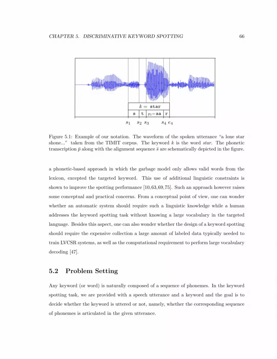
CHAPTER 5. DISCRIMINATIVE KEYWORD SPOTTING 66
s1 s2 s3 s4
star
s t aa r
e4
k =p3 =
Figure 5.1: Example of our notation. The waveform of the spoken utterance “a lone starshone...” taken from the TIMIT corpus. The keyword k is the word star. The phonetictranscription p along with the alignment sequence s are schematically depicted in the figure.
a phonetic-based approach in which the garbage model only allows valid words from the
lexicon, excepted the targeted keyword. This use of additional linguistic constraints is
shown to improve the spotting performance [10,63,69,75]. Such an approach however raises
some conceptual and practical concerns. From a conceptual point of view, one can wonder
whether an automatic system should require such a linguistic knowledge while a human
addresses the keyword spotting task without knowing a large vocabulary in the targeted
language. Besides this aspect, one can also wonder whether the design of a keyword spotting
should require the expensive collection a large amount of labeled data typically needed to
train LVCSR systems, as well as the computational requirement to perform large vocabulary
decoding [47].
5.2 Problem Setting
Any keyword (or word) is naturally composed of a sequence of phonemes. In the keyword
spotting task, we are provided with a speech utterance and a keyword and the goal is to
decide whether the keyword is uttered or not, namely, whether the corresponding sequence
of phonemes is articulated in the given utterance.

CHAPTER 5. DISCRIMINATIVE KEYWORD SPOTTING 67
Formally, we represent a speech signal as a sequence of acoustic feature vectors x =
(x1, . . . ,xT ), where xt ∈ X ⊂ Rd for all 1 ≤ t ≤ T . We denote a keyword by k ∈ V,
where V is a lexicon of words. Each keyword k is composed of a sequence of phonemes
pk = (p1, . . . , pL), where pl ∈ P for all 1 ≤ l ≤ L and P is the domain of the phoneme
symbols. We denote by P∗ the set of all finite length sequences over P. Our goal is to
learn a keyword spotter, denoted f , which takes as input the pair (x, pk) and returns a real
value expressing the confidence that the targeted keyword k is uttered in x. That is, f is a
function from X ∗ × P∗ to the set R. The confidence score outputted by f for a given pair
(x, pk) can then be compared to a threshold b to actually determine whether pk is uttered
in x. Let us further define the alignment of a phoneme sequence to a speech signal. We
denote by sl ∈ N the start time of phoneme pl (in frame units), and by el ∈ N the end
time of phoneme pl. We assume that the start time of phoneme pl+1 is equal to the end
time of phoneme pl, that is, el = sl+1 for all 1 ≤ l ≤ L − 1. The alignment sequence sk
corresponding to the phonemes sequence pk is a sequence of start-times and an end-time,
sk = (s1, . . . , sL, eL), where sl is the start-time of phoneme pl and eL is the end-time of the
last phoneme pL. An example of our notation is given in Figure 5.1.
The performance of a keyword spotting system is often measured by the Receiver Oper-
ating Characteristics (ROC) curve, that is, a plot of the true positive (spotting a keyword
correctly) rate as a function of the false positive (mis-spotting a keyword) rate (see for ex-
ample [4,41,68]). The points on the curve are obtained by sweeping the decision threshold
b from the most positive confidence value outputted by the system to the most negative
one. Hence, the choice of b represents a trade-off between different operational settings,
corresponding to different cost functions weighing false positive and false negative errors.
Assuming a flat prior over all these cost functions, a criterion to identify a good keyword
spotting system that would be good on average for all these settings could be to select
the one maximizing the area under the ROC curve (AUC). In the following we propose an
algorithm which directly aims at maximizing the AUC.

CHAPTER 5. DISCRIMINATIVE KEYWORD SPOTTING 68
5.3 A Large Margin Approach for Keyword Spotting
In this section we describe a discriminative supervised algorithm for learning a spotting
function f from a training set of examples. Our construction is based on a set of predefined
feature functions {φ}nj=1. Each feature function is of the form φj : X ∗ × P∗ × N∗ → R
. That is, each feature function takes as input an acoustic representation of a speech
utterance x ∈ X ∗, together with a phoneme sequence pk ∈ P∗ of the keyword k, and a
candidate alignment sequence sk ∈ N∗ into an abstract vector-space, and returns a scalar
in R which, intuitively, represents the confidence in the suggested alignment sequence given
the keyword phoneme sequence pk. For example, one element of the feature function can
sum the number of times phoneme p comes after phoneme p′, while other elements of the
feature function may extract properties of each acoustic feature vector xt provided that
phoneme p is pronounced at time t. The description of the concrete form of the feature
functions is differed to Section 5.6.
Our goal is to learn a keyword spotter f , which takes as input a sequence of acoustic
features x, a keyword pk, and returns a confidence value in R. The form of the function f
we use is
f(x, pk) = maxs
w · φ(x, pk, s) , (5.1)
where w ∈ Rn is a vector of importance weights (“model parameters”) that should be
learned and φ ∈ Rn is a vector function composed out of the feature functions φj . In other
words, f returns a confidence prediction about the existence of the keyword in the utterance
by maximizing a weighted sum of the scores returned by the feature function elements
over all possible alignment sequences. The maximization defined by Equation (5.1) is over
an exponentially large number of alignment sequences. Nevertheless, as in HMMs, if the
feature functions φ are decomposable, the maximization in Equation (5.1) can be efficiently
calculated using a dynamic programming procedure.
Recall that we would like to obtain a system that maximizes the AUC on unseen data. In
order to do so, we will maximize the AUC over a large set of training examples. In Section 5.5
we show that our algorithm which maximizes the AUC over the training set is likely to

CHAPTER 5. DISCRIMINATIVE KEYWORD SPOTTING 69
maximizes the AUC over an unseen data as well. Let us consider two sets of examples.
Denote by X+k a set of speech utterances in which the keyword k is uttered. Similarly,
denote by X−k a set of speech utterances in which the keyword k is not uttered. The AUC
for keyword k can be written in the form of the Wilcoxon-Mann-Whitney statistic [17] as
Ak =1
|X+k ||X
−k |
∑x+∈X+
k
∑x−∈X−k
1{f(x+,pk)>f(x−,pk)}, (5.2)
where | · | refers to the cardinality of a set, and 1{·} refers to the indicator function, that
is, 1{π} is 1 whenever the predicate π is true and 0 otherwise. Thus, Ak estimates the
probability that the score assigned to an utterance that contains the keyword k is greater
than the score assigned to an utterance which does not contain it. Hence, the average AUC
over the set of keywords V can be written as
A =1|V|∑k∈V
Ak =1|V|∑k∈V
1|X+k ||X
−k |
∑x+∈X+
k
∑x−∈X−k
1{f(x+,pk)>f(x−,pk)}. (5.3)
We now describe a large margin approach for learning the weight vector w, which defines
the keyword spotting function as in Equation (5.1), from a training set S of examples. Each
example in the training set S is composed of a keyword phoneme sequence pk, an utterance
x+ ∈ X+k in which the keyword k is uttered, an utterance x− ∈ X−k in which the keyword k
is not uttered, and an alignment sequence sk that corresponds to the location of the keyword
in x+. Overall we have m examples, that is, S = {(pk1 , x+1 , x
−1 , s
k11 ), . . . , (pkm , x+
m, x−m, s
kmm )}.
We assume that we have access to the correct alignment sk of the phonemes sequence pk
for each training utterance x+ ∈ X+k . This assumption is actually not restrictive since such
an alignment can be inferred relying on an alignment algorithm [40].
Similar to the SVM algorithm for binary classification [18, 73], our approach for choos-
ing the weight vector w is based on the idea of large-margin separation. Theoreti-
cally, our approach can be described as a two-step procedure: first, we construct the
vectors φ(x+i , p
ki , skii ) and φ(x−i , p
ki , s) in the vector space Rn based on each instance
(pki , x+i , x
−i , s
kii ), and each possible alignment sequence s for the negative sequence x−i .

CHAPTER 5. DISCRIMINATIVE KEYWORD SPOTTING 70
Second, we find a vector w ∈ Rn, such that the projection of vectors onto w ranks the
vectors constructed in the first step above according to their quality. Ideally, for any key-
word ki ∈ Vtrain, for every instance pair (x+i , x
−i ) ∈ X+
ki× X−ki
, we would like the following
constraint to hold
w · φ(x+i , p
ki , skii )−max
sw · φ(x−i , p
ki , s) ≥ 1 ∀i . (5.4)
That is, w should rank the utterance that contains the keyword above any utterance that
does not contain it by at least 1. Moreover, we even consider the best alignment of the
keyword within the utterance that does not contain it. We refer to the difference w ·
φ(x+i , p
ki , skii )−maxs w ·φ(x−i , p
ki , s) as the margin of w with respect to the best alignment
of the keyword k in the utterance that does not contain it. Note that if the prediction of
w is incorrect then the margin is negative. Naturally, if there exists a w satisfying all
the constraints Equation (5.4), the margin requirements are also satisfied by multiplying
w by a large scalar. The SVM algorithm solves this problem by selecting the weights w
minimizing 12‖w‖
2 subject to the constraints given in Equation (5.4), as it can be shown
that the solution with the smallest norm is likely to achieve better generalization [73].
In practice, it might be the case that the constraints given in Equation (5.4) cannot be
satisfied. To overcome this obstacle, we follow the soft SVM approach [18, 73] and define
the following hinge-loss function,
`(w; (pk, x+, x−, sk)) =1
|X+ki||X−ki
|
[1−w · φ(x+, pk, sk) + max
sw · φ(x−, pk, s)
]+,
(5.5)
where [a]+ = max{0, a}. The hinge loss measures the maximal violation for any of the
constraints given in Equation (5.4). The soft SVM approach for our problem is to choose
the vector w? which minimizes the following optimization problem
w? = argminw
12‖w‖2 + C
m∑i=1
`(w; (pki , x+i , x
−i , s
kii )) , (5.6)

CHAPTER 5. DISCRIMINATIVE KEYWORD SPOTTING 71
where the parameter C serves as a complexity-accuracy trade-off parameter: a low value of
C favors a simple model, while a large value of C favors a model which solves all training
constraints (see [20]). Solving the optimization problem given in Equation (5.6) is expensive
since it involves a maximization for each training example. Most of the solvers for this
problem, like SMO [54], iterate over the whole dataset several times until convergence. In
the next section, we propose a slightly different method, which visits each example only
once, and is based on our previous work [19].
5.4 An Iterative Algorithm
We now describe a simple iterative algorithm for learning the weight vector w. The algo-
rithm receives as input a set of training examples S = {(pki , x+i , x
−i , s
kii )}mi=1 and examines
each of them sequentially. Initially, we set w = 0. At each iteration i, the algorithm updates
w according to the current example (pki , x+i , x
−i , s
kii ) as we now describe. Denote by wi−1
the value of the weight vector before the ith iteration. Let s′ be the predicted alignment
for the negative utterance, x−i , according to wi−1,
s′ = arg maxs
wi−1 · φ(x−i , pki , s) . (5.7)
Let us define the normalized difference between the feature functions of the acoustic
sequence in which the keyword is uttered and the feature functions of the acoustic sequence
in which the keyword is not uttered as ∆φi, that is,
∆φi =1
|X+ki||X−ki
|
(φ(x+
i , pki , ski)− φ(x−i , p
ki , s′)). (5.8)
The normalization factor is a result of our goal to minimize the average AUC (see Sec-
tion 5.5). We set the next weight vector wi to be the minimizer of the following optimization

CHAPTER 5. DISCRIMINATIVE KEYWORD SPOTTING 72
problem,
minw∈Rn,ξ≥0
12‖w −wi−1‖2 + C ξ (5.9)
s.t. w ·∆φ ≥ 1−ξ ,
where C serves as a complexity-accuracy trade-off parameter (see [19]) and ξ is a non-
negative slack variable, which indicates the loss of the ith example. Intuitively, we would
like to minimize the loss of the current example, i.e., the slack variable ξ, while keeping the
weight vector w as close as possible to the previous weight vector wi−1. The constraint
makes the projection of the sequence that contains the keyword onto w higher than the
projection of the sequence that does not contains it onto w by at least 1. It can be shown
(see [19] that the solution to the above optimization problem is
wi = wi−1 + αi∆φi . (5.10)
The value of the scalar αi is based on the difference ∆Φi, the previous weight vector wi−1,
and a parameter C. Formally,
αi = min{C,
[1−wi−1 ·∆φi]+‖∆φi‖2
}. (5.11)
The optimization problem given in Equation (5.9) is based on ongoing work on online
learning algorithms appearing in [19]. Based on this work, it is shown in Section 5.5 that,
under some mild technical conditions, the cumulative performance of the iterative proce-
dure, i.e., 1m
∑mi=1 1{wi·∆φi>0} is likely to be high. Moreover, it can further be shown that
if the cumulative performance of the iterative procedure is high, there exists at least one
weight vector among the vectors {w1, . . . ,wm} which attains high averaged performance on
unseen examples as well, that is, there exists a vector which attains high averaged AUC over
a set of unseen examples. To find this weight vector, we simply calculate the averaged loss
attained by each of the weight vectors on a validation set. A pseudo-code of our algorithm

CHAPTER 5. DISCRIMINATIVE KEYWORD SPOTTING 73
Input: training set S = {(pki , x+i , x
−i , s
ki)}mi=1; validation set Sval; parameter CInitialize: w0 = 0For i = 1, . . . ,m
Predict: s′ = arg maxs wi−1 · φ(x−i , pki , s)
Set: ∆φi = φ(x+i , p
ki , ski)− φ(x−i , pki , s′)
If wi−1 ·∆φi < 1
Set: αi = min{C ,
1−wi−1 ·∆φi
‖∆φi‖2
}Update: wi = wi−1 + αi ·∆φi
Output: The weight vector w∗ which achieves best AUC performance on the validationset Sval.
Figure 5.2: An iterative algorithm.
is given in Figure 5.2.
In the case the user would like to select a threshold b that would ensure a specific
requirement in terms of true positive rate or false negative rate, a simple cross-validation
procedure [5] would consist in selecting the confidence value given by our model at the
point of interest over the ROC curve plotted for some validation utterances of the targeted
keyword.
5.5 Theoretical Analysis
In this section, we show that the iterative algorithm given in Section 5.4 maximizes the
cumulative AUC, defined as
A =1m
m∑i=1
1{wi·φ(x+i ,p
ki ,ski )≥wi·φ(x−,pki ,s′i)}. (5.12)
Our first theorem shows that the area above the curve, i.e. 1 − A, is smaller than the
average loss of the solution of the SVM problem defined in Equation (5.6). That is, the
cumulative AUC, generating by the iterative algorithm is going to be large, given that the
loss of the SVM solution (or any other solution) is small, and that the number of examples,

CHAPTER 5. DISCRIMINATIVE KEYWORD SPOTTING 74
m, is sufficiently large.
Theorem 5.5.1.: Let S = {(pki , x+i , x
−i , s
kii )}mi=1 be a set of training examples and assume
that for all k, x and s we have that ‖φ(x, pk, s)‖ ≤ 1. Let w? be the optimum of the SVM
problem given in Equation (5.6). Let w1, . . . ,wm be the sequence of weight vectors obtained
by the algorithm in Figure 5.2 given the training set S. Then,
1− A ≤ 1m‖w?‖2 +
2Cm
m∑i=1
`(w?; (pki , x+i , x
−i , s
ki)). (5.13)
where C > 1 and A is the cumulative AUC.
Proof. The proof of the theorem relies on Lemma 1 and Theorem 4 in [19]. Lemma 1 in [19]
implies that,m∑i=1
αi(2`i − αi‖∆φi‖2 − 2`?i
)≤ ‖w?‖2. (5.14)
Now if the algorithm makes a prediction mistake, i.e., predicts that an utterance that does
not contain the keyword has a greater confidence than another utterance that does contain
it, then `i ≥ 1. Using the assumption that ‖φ(x, pk, s)‖ ≤ 1 and the definition of αi given in
Equation (5.11), when substituting [1−wi−1 ·∆φi]+ for `i in its denominator, we conclude
that if a prediction mistake occurs then it holds that
αi`i ≥ min{
`i∆φi
, C
}≥ min {1, C} = 1. (5.15)
Summing over all the prediction mistakes made on the entire training set S and taking into
account that αi`i is always non-negative. it holds that
m∑i=1
αi`i ≥m∑i=1
1{wi·φ(x+i ,p
ki ,ski )≤wi·φ(x−,pki ,s′i)}. (5.16)
Again using the definition of αi, we know that αi`?i ≤ C`?i and that αi‖∆φi‖2 ≤ `i. Plugging

CHAPTER 5. DISCRIMINATIVE KEYWORD SPOTTING 75
these two inequalities and Equation (5.16) into Equation (5.14) we get
m∑i=1
1{wi·φ(x+i ,p
ki ,ski )≤wi·φ(x−,pki ,s′i)}≤ ‖w?‖2 + 2C
m∑i=1
`?i . (5.17)
The theorem follows by replacing the sum over prediction mistakes to a sum over prediction
hits and pluging-in the definition of the cumulative AUC given in Equation (5.12).
The next theorem states that the output of our algorithm is likely to have good gener-
alization, i.e. the expected value of the AUC resulted from decoding on unseen test set is
likely to be large.
Theorem 5.5.2.: Under the same conditions of Theorem 5.5.1. Assume that the training
set S and the validation set Sval are both sampled i.i.d. from a distribution Q. Denote by
mval the size of the validation set. With probability of at least 1− δ we have
1− A = EQ[1{f(x+
i ,pki )≤f(x−,pki )}
]= PrQ
[f(x+
i , pki) ≤ f(x−, pki)
]≤
1m
m∑i=1
`(w?; (pki , x+i , x
−i , s
ki)) +‖w?‖2
m+
√2 ln(2/δ)√
m+
√2 ln(2m/δ)√mval
, (5.18)
where A is the mean AUC defined as A = EQ[1{f(x+
i ,pki )>f(x−,pki )}
].
Proof. Denote the risk of keyword spotter f by
risk(f) = E[1{f(x+
i ,pki )≤f(x−,pki )}
]= P
[f(x+
i , pki) ≤ f(x−, pki)
]Proposition 1 in [12] implies that with probability of at least 1 − δ1 the following bound
holds,1m
m∑i=1
risk(fi) ≤1m
m∑i=1
1{fi(x+i ,p
ki )≤fi(x−,pki )} +
√2 ln(1/δ1)√
m.
Combining this fact with Theorem 5.5.1 we obtain that,
1m
m∑i=1
risk(fi) ≤2Cm
m∑i=1
`?i +‖w?‖2
m+
√2 ln (1/δ1)√
m. (5.19)

CHAPTER 5. DISCRIMINATIVE KEYWORD SPOTTING 76
The left-hand side of the above inequality upper bounds risk(f?), where f? =
arg minfirisk(fi). Therefore, among the finite set of keyword spotting functions, F =
{f1, . . . , fm}, there exists at least one keyword spotting function (for instance the function
f?) whose true risk is bounded above by the right hand side of Equation (5.19). Recall that
the output of our algorithm is the keyword spotter f ∈ F , which minimizes the average cost
over the validation set Sval. Applying Hoeffding inequality together with the union bound
over F we conclude that with probability of at least 1− δ2,
risk(f) ≤ risk(f?) +
√2 ln (m/δ2)
mval,
where mval = |Sval|. We have therefore shown that with probability of at least 1 − δ1 − δ2
the following inequality holds,
risk(f) ≤ 1m
m∑i=1
`?i +‖w?‖2
m+
√2 ln(1/δ1)√
m+
√2 ln(m/δ2)√mval
.
Setting δ1 = δ2 = δ/2 concludes our proof.
5.6 Feature Functions
In this section we present the implementation details of our learning approach for the task
of keyword spotting. Recall that our construction is based on a set of feature functions,
{φj}nj=1, which maps an acoustic-phonetic representation of a speech utterance as well as
a suggested alignment sequence into a vector-space. In order to make this section more
readable we omit the keyword index k.
We introduce a specific set of base functions, which is highly adequate for the keyword
spotting problem. We utilize seven different feature functions (n = 7). These feature
functions are used for defining our keyword spotting function f(x, p) as in Equation (5.1).
Note that the same set of feature functions found also to be also useful in the task of
speech-to-phoneme alignment (see Chapter 3).

CHAPTER 5. DISCRIMINATIVE KEYWORD SPOTTING 77
Our first four feature functions aim at capturing transitions between phonemes. These
feature functions are the distance between frames of the acoustic signal at both sides of
phoneme boundaries as suggested by an alignment sequence s. The distance measure we
employ, denoted by d, is the Euclidean distance between feature vectors. Our underlying
assumption is that if two frames, xt and xt′ , are derived from the same phoneme then
the distance d(xt,xt′) should be smaller than if the two frames are derived from different
phonemes. Formally, our first four feature functions are defined as
φj(x, p, s) =|p|−1∑i=2
d(x−j+si ,xj+si), j ∈ {1, 2, 3, 4} . (5.20)
If s is the correct timing sequence then distances between frames across the phoneme change
points are likely to be large. In contrast, an incorrect phoneme start time sequence is likely
to compare frames from the same phoneme, often resulting in small distances.
The fifth feature function we use is built from a frame-wise phoneme classifier described
in [23]. Formally, for each phoneme event p ∈ P and frame x ∈ X , there is a confidence,
denoted gp(x), that the phoneme p is pronounced in the frame x. The resulting feature func-
tion measures the cumulative confidence of the complete speech signal given the phoneme
sequence and their start-times,
φ5(x, p, s) =|p|∑i=1
si+1−1∑t=si
gpi(xt) . (5.21)
Our next feature function scores alignment sequences based on phoneme durations.
Unlike the previous feature functions, the sixth feature function is oblivious to the speech
signal itself. It merely examines the length of each phoneme, as suggested by s, compared
to the typical length required to pronounce this phoneme. Formally,
φ6(x, p, s) =|p|∑i=1
log N (si+1 − si; µpi , σpi) , (5.22)
where N is a Normal probability density function with mean µp and standard deviation σp.

CHAPTER 5. DISCRIMINATIVE KEYWORD SPOTTING 78
In our experiments, we estimated µp and σp from the training set (see Section 5.7).
Our last feature function exploits assumptions on the speaking rate of a speaker. In-
tuitively, people usually speak in an almost steady rate and therefore a timing sequence in
which speech rate is changed abruptly is probably incorrect. Formally, let µp be the average
length required to pronounce the pth phoneme. We denote by ri the relative speech rate,
ri = (si+1 − si)/µpi . That is, ri is the ratio between the actual length of phoneme pi as
suggested by s to its average length. The relative speech rate presumably changes slowly
over time. In practice the speaking rate ratios often differ from speaker to speaker and
within a given utterance. We measure the local change in the speaking rate as (ri − ri−1)2
and we define the feature function φ7 as the local change in the speaking rate,
φ7(x, p, s) =|p|∑i=2
(ri − ri−1)2 . (5.23)
Each of the feature functions is normalized by the number of frames in the speech
utterance, and each of the feature functions is weighted be a fixed constant, {βj}7j=1. The
constants are determined so as to maximize performance over a validation set.
5.7 Experimental Results
To validate the effectiveness of the proposed approach we performed experiments with the
TIMIT corpus. We divided the training portion of TIMIT (excluding the SA1 and SA2
utterances) into three disjoint parts containing 500, 80 and 3116 utterances. The first part
of the training set was used for learning the functions gp (Equation (5.21)), which define the
feature function φ5. Those functions were learned by the algorithm described in [23] using
the MFCC+∆+∆∆ acoustic features and a Gaussian kernel with parameter σ = 6.24.
The second set of 80 utterances formed the validation set needed for our keyword spot-
ting algorithm. The set was built out of a set of 40 keywords randomly chosen from the
TIMIT lexicon. The 80 utterances were chosen by pairs: one utterance in which the key-
word was uttered and another utterance in which the keyword was not uttered. Finally, we

CHAPTER 5. DISCRIMINATIVE KEYWORD SPOTTING 79
ran our iterative algorithm on the rest of the utterances in the training set. The value of
the parameter C was set to be 1.
We compared the results of our method to the HMM approach, where each phoneme
was represented by a simple left-to-right HMM of 5 emitting states with 40 diago-
nal Gaussians. These models were enrolled as follows: first the HMMs were initial-
ized using K-means, and then enrolled independently using EM. The second step, of-
ten called embedded training, re-enrolls all the models by relaxing the segmentation con-
straints using a forced alignment. Minimum values of the variances for each Gaus-
sian were set to 20% of the global variance of the data. All HMM experiments
garbage HMM
keyword HMM
. . .
. . .
Figure 5.5: HMM topology for keyword
spotting.
were done using the Torch package [16]. All
hyper-parameters including number of states,
number of Gaussians per state, variance floor-
ing factor, were tuned using the validation set.
Keyword detection was performed with a
new HMM composed of two sub HMM mod-
els, the keyword model and the garbage model,
as depicted in Figure 5.5. The keyword model
was an HMM which estimated the likelihood of
an acoustic sequence given that the sequence
represented the keyword phoneme sequence.
The garbage model was an HMM composed of
phoneme HMMs fully connected to each others,
which estimated the likelihood of any acoustic
sequence. The overall HMM fully connected the
keyword model and the garbage model. The detection of a keyword given a test utterance
was performed through a best path search, were an external parameter of the prior keyword
probability was added to the keyword sub HMM model. The best path found by Viterbi
decoding on the overall HMM either passed through the keyword model (in which case the

CHAPTER 5. DISCRIMINATIVE KEYWORD SPOTTING 80
0 0.2 0.4 0.6 0.8 10
0.2
0.4
0.6
0.8
1
false positive rate
true
posit
ive
rate
discriminativeHMM
Figure 5.3: ROC curves of the discriminative algorithm and the HMM approach, trainedon the TIMIT training set and tested on 80 keywords from TIMIT test set. The AUC ofthe ROC curves is 0.99 and 0.96 for the discriminative algorithm and the HMM algorithm,respectively.
0 0.2 0.4 0.6 0.8 10
0.2
0.4
0.6
0.8
1
false positive rate
true
posit
ive
rate
discriminativeHMM
Figure 5.4: ROC curves of the discriminative algorithm and the HMM approach, trainedon the TIMIT training set and tested on 80 keywords from WSJ test set. The AUC ofthe ROC curves is 0.94 and 0.88 for the discriminative algorithm and the HMM algorithm,respectively.

CHAPTER 5. DISCRIMINATIVE KEYWORD SPOTTING 81
Table 5.1: The AUC of the discriminative algorithm compared to the HMM in the experi-ments.
Discriminative Algo. HMMCorpus AUC AUCTIMIT 0.99 0.96WSJ 0.94 0.88
keyword was said to be uttered) or not (in which case the keyword was not in the acoustic
sequence). Swiping the prior keyword probability parameters set the trade-off between the
true positive rate and the false positive rate.
The test set was composed of 80 randomly chosen keywords, distinct from the keywords
of the training and validation sets. For each keyword, we randomly picked at most 20
utterances in which the keyword was uttered and at most 20 utterances in which it was not
uttered. Note that the number of test utterances in which the keyword was uttered was not
always 20, since some keywords were uttered less than 20 times in the whole TIMIT test set.
Both the discriminative algorithm and the HMM based algorithm was evaluated against the
test data. The results are reported as averaged ROC curves in Figure 5.3. The AUC of
the ROC curves is 0.99 and 0.96 for the discriminative algorithm and the HMM algorithm,
respectively. In order to check whether the advantage over the averaged AUC could be due
to a few keyword, we ran the Wilcoxon test. At the 95% confidence level, the test rejected
this hypothesis, showing that our model indeed brings a consistent improvement on the
keyword set.
The next experiment examines the robustness of the proposed algorithm. We compared
the performance of the proposed discriminative algorithm and of the HMM on the WSJ
corpus [52]. Both systems were trained on the TIMIT corpus as describe above and tested
on the same 80 keywords. For each keyword we randomly picked at most 20 utterances from
the si tr s portion of the WSJ corpus. The ROC curves are given in Figure 5.4. The
AUC of the ROC curves is 0.94 and 0.88 for the discriminative algorithm and the HMM
algorithm, respectively. With more than 99% confidence, the Wilcoxon test rejected the

CHAPTER 5. DISCRIMINATIVE KEYWORD SPOTTING 82
hypothesis that the difference between the two models was due to only a few keywords.
A summary of the results of both experiments is given in Table 5.1. Close look on
both experiments, we see that the discriminative algorithm outperforms the HMM in terms
of AUC. This indeed validates our theoretical analysis that our algorithm maximizes the
AUC. Moreover, the discriminative algorithm outperforms the HMM in all point of the
ROC curve, meaning that it has better true positive rate for every given false negative rate.

Chapter 6
Discussion
In this thesis we presented several algorithms that set the basis for a large margin kernel-
based acoustic model for continuous speech recognition. We demonstrated the usefulness
of different aspects of the acoustic model on the TIMIT corpus. Along the way, we gave
theoretical support to the algorithms given, and showed that they minimize the loss over
the training set and the test set.
We started with the hierarchical phoneme classifier. We proposed a frame-based multi-
class classifier which imposes a notion of “severity” of prediction errors in accordance with
a pre-defined hierarchical phoneme structure. We describe online and batch algorithms for
solving the constrained optimization problem represents the hierarchical multiclass phoneme
classifier. We derived a worst case loss-bound for the online algorithm and provided gener-
alization analysis for its batch counterpart. We demonstrated the merits of our approach
with a series of experiments. The algorithm is the basis of the speech-to-phoneme alignment
and the keyword spotting algorithms.
Next, we presented a discriminative algorithm for learning a speech-to-phoneme align-
ment function from a training set of examples. The contribution of our algorithm is twofold.
First, we showed for the first time how a large margin algorithm can be used to model the
problem of speech-to-phoneme alignment. Second, we presented a simple yet effective al-
gorithm for solving the problem. Our learning algorithm is more efficient than similar
83

CHAPTER 6. DISCUSSION 84
algorithms for large margin sequence prediction (such as [70,72]), and is most adequate for
speech, in which we typically have a large number of training examples. Our learning algo-
rithm is simple to implement and entertains convergence guarantees. Moreover, we showed
both theoretical and empirical evidence demonstrating the generalization abilities of our
method. Indeed, the experiments reported above suggest that the discriminative training
requires fewer training examples than an HMM-based forced-alignment procedure.
A whole sequence phoneme recognition which is based on discriminative supervised
learning and Mercer kernels was presented after the speech-to-phoneme alignment. The
error of a phoneme recognizer is often measured in terms of the Levenshtein distance (the
minimum edit distance operations needed to transform the predicted phoneme sequence to
the true one). We proposed an algorithm that directly minimizes the Levenshtein distance
over a training set of transcribed examples and showed its generalization performances over
unseen data as well. So far, the experimental results we obtained with our method for
the task of phoneme recognition are inferior to state-of-the-art results obtained by HMMs.
However, while there has been extensive continuous effort on using HMMs for phoneme
sequence recognition, our method is rather innovative and the choice of features and kernel
operators is by no means comprehensive. We intend to utilize the full power of kernel
methods for phoneme recognition by experimenting with additional features and kernels for
our task.
Last, we showed an algorithm for keyword spotting in a discriminative way. While cur-
rent state-of-the-art are mostly based on traditional generative HMM based approaches,
we introduced a discriminative approach to keyword spotting, directly optimizing an objec-
tive function related to the area under the ROC curve, i.e., the most common measure for
keyword spotter evaluation. Compared to state-of-the-art approaches, the proposed model
showed to yield a statistically significant improvement over the TIMIT corpus. Further-
more, the very same model trained on the TIMIT corpus but tested on the WSJ corpus also
yielded a statistically significant better performance than the HMM based approach. As far
as we know, this is the first time the keyword spotting problem is addressed discriminatively.

CHAPTER 6. DISCUSSION 85
The algorithms presented in this thesis set the basic building blocks for large margin kernel
based continuous speech recognition. However, there remains a gap to be covered: these
algorithms are not sufficiently useful with regards to large vocabulary continuous speech
recognition (LVCSR). By LVCSR we mean a speech recognizer that can handle spontaneous
speech over a vocabulary size of 10,000 words and above. In the following we give a short
description of a kernel-based LVCSR model and discuss some of the open problems in its
design and implementation.
Recall that the problem of speech recognition is stated in Equation (1.1) as the problem
of finding the most likely sequence of words w′ given the acoustic feature vectors x. In its
logarithm form it can be written as
w′ = arg maxw
log P(x|w) + log P(w) ,
where P(x|w) is the probability of the acoustic features given the word sequence known
as the acoustic model, and P(w) is the probability of the sequence of words known as the
language model.
In the LVCSR setting our goal is to learn a function, which takes as input an acoustic
signal x and returns a word sequence w. The form of the function we use is
w′ = arg maxw
w · φ(x, w) ,
where w ∈ H is a vector of weights in a reproducing kernel Hilbert space H, and φ :
X ? × V? → H is a vector feature function that maps the acoustic signal x and a candidate
word sequence w to the same space H. In the same spirit of generative LVCSR, this function
can be written as a sum of the acoustic model and the language model,
w′ = arg maxw
wacoustic · φacoustic(x, w) + wlanguage · φlanguage(w) , (6.1)
where both wacoustic and wlanguage are sub-vectors of the vector w. The first term wacoustic ·
φacoustic(x, w) in the equation is the acoustic modeling, and it gives confidence for every

CHAPTER 6. DISCUSSION 86
candidate word sequence w and the given acoustic signal x that is spoken.
The second term wlanguage · φlanguage(w) in Equation (6.1) is the language model. Tra-
ditionally, the language model assigns a probability to a sequence of words by means of a
probability distribution. In the discriminative setting, the language model gives confidence
to a string of words in a natural language. Collins and his colleagues [58] described dis-
criminative language modeling for a large vocabulary speech recognition task which would
be suitable for the above setting. Another way to build a discriminative language model is
by using prediction suffix trees (PSTs) [24,62] as demonstrated in [53].
The acoustic model and the language mode in Equation (6.1) are trained discriminatively
together as to minimize the Levenshtein distance between the predicted word sequence and
the correct one, as proposed in Chapter 4. We now describe a simple iterative algorithm
for learning the weight vectors wacoustic and wlanguage. The algorithm receives as input a
training set S = {(x1, w1), . . . , (xm, wm)} of examples. Each example is constituted of a
spoken acoustic signal xi and its corresponding word sequence wi. At each iteration the
algorithm updates wacoustic and wlanguage according to the ith example in S as we now
describe. Denote by wacoustici−1 and wlanguage
i−1 the value of the weight vectors before the ith
iteration. Let w′i be the predicted word sequence for the ith example according to wacoustici−1
and wlanguagei−1 ,
w′i = arg maxw
wacoustic · φacoustic(xi, wi) + wlanguage · φlanguage(wi) . (6.2)
Denote by γ(w, w′) the Levenshtein distance between the correct word sequence w and the
predicted word sequence w′. We set the next weight vectors wacoustici and wlanguage
i to be
the minimizer of the following optimization problem,
minw∈H,ξ≥0
12‖wacoustic −wacoustic
i−1 ‖2 +12‖wlanguage −wlanguage
i−1 ‖2 + Cξ (6.3)
s.t. wacoustic · φacoustic(xi, wi) + wlanguage · φlanguage(wi) −
wacoustic · φacoustic(xi, w′i) − wlanguage · φlanguage(w′i) ≥ γ(wi, w′i)− ξ .

CHAPTER 6. DISCUSSION 87
This process iterates over all training examples in S.
Under some mild technical conditions, it can be shown that the cumulative Levenshtein
distance of an iterative procedure ,∑m
i=1 γ(wi, w′i), is likely to be small. Moreover, it can be
shown [12] that if the cumulative Levenshtein distance of the iterative procedure is small,
there exists among the vectors {w1, . . . ,wm} at least one weight vector which attains small
averaged Levenshtein distance on unseen examples as well.
The feature functions φacoustic(x, w) gets the acoustic representation, x, and a candi-
date sequence of words, w, and returns a scalar which represents the confidence in the
suggested word sequence. Such a vector feature function that depends on the candidate
word sequence can be hardly found for a small vocabulary recognizer and cannot be found
for a large vocabulary recognizer. We would therefore like to express the vector feature
function in terms of a candidate phoneme sequence, which is the orthographic transcrip-
tion of the candidate word sequence. Once we have a vector feature function that depends
on a phoneme sequence and on an acoustic signal we can use the set of feature functions
and Mercer kernels proposed in Sections 3.7 and 4.4. However, although that set of fea-
ture functions is based on a phoneme sequence, it is also based on the start-time sequence.
While there is a function that maps a word to a phoneme sequence called pronunciation
dictionary, there is no function that can map a word to its correct start-time sequence. One
can use the speech-to-phoneme alignment function learned in Chapter 3, but the meaning
is another pass on the training set. In fact, we can try to find the best alignment of the
phoneme sequence with the speech signal, but that would lead to a non-convex optimization
problem, and no theoretical guarantee on the minimization of the Levenshtein distance.
The algorithm presented here is very similar to the one presented for phoneme sequence
recognition. The real difference between the two, however, is the way one performs the
search. While in the phoneme recognizer, searching over all possible phoneme sequence is
feasible with a Viterbi algorithm, in the word sequence recognizer, running over all possible
word sequences is not feasible. There are common techniques that efficiently and heuristi-
cally handle the search, such as the beam search [32] and the A∗ stack search [51]. Although
both methods are popular in LVCSR systems, they have difficulties in implementing n-gram

CHAPTER 6. DISCUSSION 88
language models where n is larger than 3 (see [35,49] for a detailed discussion). A method
that is suitable for the language model proposed here is the fast match [2].
Concluding the discussion, we would like to quote a short phrase from a paper by Bourlard,
Hermansky and Morgan [7], who claimed that radical innovations are necessary to address
the problem of speech recognition:
Permitting an initial increase in error rate can be useful, as long as three conditions are
fulfilled:
(1) solid theoretical or empirical motivations,
(2) sound methodology (so that something can be learned from the results), and
(3) deep understanding of state-of-the-art systems and of the specificity of the new ap-
proach...
The development of new technologies will often initially result in a significant increase in
speech recognition error rates before becoming competitive with or better than the best current
systems.
Bibliography
[1] J. B. Allen. Articulation and Intelligibility. Morgan & Claypool, 2005.
[2] L.R. Bahl, S.V. De Gennaro, P.S. Gopalakrishnan, and R.L. Mercer. A fast approxi-
mate acoustic match for large vocabulary speech recognition. IEEE Transactions on
Speech and Audio Processing, 1(1):59–67, 1993.
[3] L. E. Baum, T. Petrie, G. Soules, and N. Weiss. A maximization technique occurring
in the statistical analysis of probabilistic functions of Markov chains. The Annals of
Mathematical Statistics, 41(1):164–171, 1970.
[4] Y. Benayed, D. Fohr, J.-P. Haton, and G. Chollet. Confidence measure for keyword
spotting using support vector machines. In Proc. of International Conference on Audio,
Speech and Signal Processing, 2004.
[5] S. Bengio, J. Marethoz, and M. Keller. The expected performance curve. In Proceedings
of the 22nd International Conference on Machine Learning, 2005.
[6] H. Bourlard, B. D’Hoore, and J.-M. Boite. Optimizing recognition and rejection per-
formance in wordspotting systems. In Proc. of International Conference on Audio,
Speech and Signal Processing, pages 373–376, 1994.
[7] H. Bourlard, H. Hermansky, and N. Morgan. Towards increasing speech recognition
error rates. Speech Communication, 18:205–231, 1996.
[8] S. Boyd and L. Vandenberghe. Convex Optimization. Cambridge University Press,
2004.
89

BIBLIOGRAPHY 90
[9] F. Brugnara, D. Falavigna, and M. Omologo. Automatic segmentation and labeling of
speech based on hidden markov models. Speech Communication, 12:357–370, 1993.
[10] P.S. Cardillo, M. Clements, and M.S. Miller. Phonetic searching vs. lvcsr: How to find
what you really want in audio archives. International Journal of Speech Technology,
5:9–22, 2002.
[11] Y. Censor and S.A. Zenios. Parallel Optimization: Theory, Algorithms, and Applica-
tions. Oxford University Press, New York, NY, USA, 1997.
[12] N. Cesa-Bianchi, A. Conconi, and C. Gentile. On the generalization ability of on-
line learning algorithms. IEEE Transactions on Information Theory, 50(9):2050–2057,
September 2004.
[13] R. Chengalvarayan and L. Deng. Speech trajectory discrimination using the minimum
classification error learning. IEEE Trans. Speech and Audio Proc., 6(6):505–515, 1998.
[14] P. Clarkson and P. Moreno. On the use of support vector machines for phonetic
classification. In Proceedings of the International Conference on Acoustics, Speech and
Signal Processing 1999, Phoenix, Arizona, 1999.
[15] M. Collins. Discriminative training methods for hidden markov models: Theory and ex-
periments with perceptron algorithms. In Conference on Empirical Methods in Natural
Language Processing, 2002.
[16] R. Collobert, S. Bengio, and J. Mariethoz. Torch: a modular machine learning software
library. IDIAP-RR 46, IDIAP, 2002.
[17] C. Cortes and M. Mohri. Confidence intervals for the area under the ROC curve. In
Advances in Neural Information Processing Systems 17, 2004.
[18] C. Cortes and V. Vapnik. Support-vector networks. Machine Learning, 20(3):273–297,
September 1995.

BIBLIOGRAPHY 91
[19] K. Crammer, O. Dekel, J. Keshet, S. Shalev-Shwartz, and Y. Singer. Online passive
aggressive algorithms. Journal of Machine Learning Research, 7, 2006.
[20] N. Cristianini and J. Shawe-Taylor. An Introduction to Support Vector Machines.
Cambridge University Press, 2000.
[21] T. Dean and K. Kanazawa. A model for reasoning about persistence and causation.
Computational Intelligence, 5(3):142–150, 1989.
[22] O. Dekel, J. Keshet, and Y. Singer. Large margin hierarchical classification. In Pro-
ceedings of the Twenty-First International Conference on Machine Learning, 2004.
[23] O. Dekel, J. Keshet, and Y. Singer. Online algorithm for hierarchical phoneme classi-
fication. In Workshop on Multimodal Interaction and Related Machine Learning Algo-
rithms; Lecture Notes in Computer Science, pages 146–159. Springer-Verlag, 2004.
[24] O. Dekel, S. Shalev-Shwartz, and Y. Singer. The power of selective memory: Self-
bounded learning of prediction suffix trees. In Advances in Neural Information Pro-
cessing Systems 17, 2004.
[25] J.R Deller, J.G. Proakis, and J.H.L. Hansen. Discrete-Time Processing of Speech
Signals. Prentice-Hall, 1987.
[26] A.P. Dempster, N.M. Laird, and D.B. Rubin. Maximum likelihood from incomplete
data via the EM algorithm. Journal of the Royal Statistical Society, Ser. B, 39:1–38,
1977.
[27] V. Digalakis, M. Ostendorf, and J. R. Rohlicek. Fast algorithms for phone classification
and recognition using segment-based models. IEEE Transactions on Signal Processing,
pages 2885–2896, dec 1992.
[28] S. T. Dumais and H. Chen. Hierarchical classification of Web content. In Proceedings
of SIGIR-00, pages 256–263, 2000.

BIBLIOGRAPHY 92
[29] Y. Erlich. On HMM based speech recognition using the MCE approach. Master’s
thesis, Techinion-Israel Institute of Technology, 1996.
[30] ETSI Standard, ETSI ES 201 108, 2000.
[31] W. D. Goldenthal. Statistical Trajectory Models for Phonetic Recognition. PhD thesis,
Massachussetts Institue of Technology, 1994.
[32] R. Haeb-Umbach and H. Ney. Improvements in beam search for 10000-word continuous-
speech recognition. IEEE Transactions on Speech and Audio Processing, 2(2):353–356,
1994.
[33] M. Herbster. Learning additive models online with fast evaluating kernels. In Proceed-
ings of the Fourteenth Annual Conference on Computational Learning Theory, pages
444–460, 2001.
[34] J.-P. Hosom. Automatic phoneme alignment based on acoustic-phonetic modeling. In
Proceedings of the Seventh International Conference on Spoken Language Processing,
pages 357–360, 2002.
[35] F. Jelinek. Statistical Methds for Speech Recognition. The MIT Press, 1998.
[36] J. Junkawitsch, G. Ruske, and H. Hoge. Efficient methods for detecting keywords in
continuous speech. In Proc. of European Conference on Speech Communication and
Technology, pages 259–262, 1997.
[37] S. Katz. Estimation of probabilities from sparsedata for the language model component
of a speech recognizer. IEEE Transactions on Acoustics, Speech and Signal Processing
(ASSP), 35(3):400–40, 1987.
[38] P. Kenny, M. Lenning, and P. Mermelstein. A linear predictive HMM for vector valued
observations with applications to speech recognition. IEEE Transactions on Speech
and Audio Processing, 38(2):220–225, 1990.

BIBLIOGRAPHY 93
[39] J. Keshet, D. Chazan, and B.-Z. Bobrovsky. Plosive spotting with margin classifiers.
In Proceedings of the Seventh European Conference on Speech Communication and
Technology, pages 1637–1640, 2001.
[40] J. Keshet, S. Shalev-Shwartz, Y. Singer, and D. Chazan. Phoneme alignment based on
discriminative learning. In Interspeech, 2005.
[41] H. Ketabdar, J. Vepa, S. Bengio, and H. Bourlard. Posterior based keyword spotting
with a priori thresholds. In Prof. of Interspeech, 2006.
[42] J. Kivinen and M. Warmuth. Exponentiated gradient versus gradient descent for linear
predictors. Information and Computation, 132(1):1–64, January 1997.
[43] D. Koller and M. Sahami. Hierarchically classifying docuemnts using very few words.
In Machine Learning: Proceedings of the Fourteenth International Conference, pages
171–178, 1997.
[44] K.-F. Lee and H.-W. Hon. Speaker independent phone recognition using hidden markov
models. IEEE Trans. Acoustic, Speech and Signal Proc., 37(2):1641–1648, 1989.
[45] L. Lemel, R. Kassel, and S. Seneff. Speech database development: Design and analysis .
Report no. SAIC-86/1546, Proc. DARPA Speech Recognition Workshop, 1986.
[46] Z. Litichever and D. Chazan. Classification of transition sounds with application to
automatic speech recognition. In EUROSPEECH, 2001.
[47] A.S. Manos and V.W. Zue. A segment-based wordspotter using phonetic filler models.
In Proc. of International Conference on Audio, Speech and Signal Processing, pages
899–902, 1997.
[48] A. K. McCallum, R. Rosenfeld, T. M. Mitchell, and A. Y. Ng. Improving text clas-
sification by shrinkage in a hierarchy of classes. In Proceedings of ICML-98, pages
359–367, 1998.

BIBLIOGRAPHY 94
[49] H. Murveit, J. Butzberger, V. Digalakis, and M. Weintraub. Large vocabulary dictation
using SRI’s deciper speech recognition: progressive search techniques. In Proc. of the
Spoken Language Systems Technology Workshop, 1993.
[50] M. Ostendorf, V.V. Digalakis, and O.A. Kimball. From hmm’s to segment models: A
unified view to stochastic modeling for speech recognition. IEEE Trans. Speech and
Audio Proc., 4(5):360–378, 1996.
[51] D.B. Paul. An essential a∗ stack decoder algorithm for continuous speech recognition
with a stochastic language model. In icassp, 1992.
[52] D.B. Paul and J.M. Baker. The design for the Wall Street Journal-based CSR corpus.
In Proc. of the International Conference on Spoken Language Processing, 1992.
[53] F. Pereira, Y. Singer, and N. Tishby. Beyond word N-grams. In Proceedings of the
Third Workshop on Very Large Corpora,, 1995.
[54] J. C. Platt. Fast training of Support Vector Machines using sequential minimal op-
timization. In B. Scholkopf, C. Burges, and A. Smola, editors, Advances in Kernel
Methods - Support Vector Learning. MIT Press, 1998.
[55] L. Rabiner and B.H. Juang. Fundamentals of Speech Recognition. Prentice Hall, 1993.
[56] L. R. Rabiner and R. W. Schafer. Digital Processing of Speech Signals. Prentice-Hall,
1978.
[57] M.G. Rahim, C.H. Lee, and B.H. Juang. Discriminative utterance verification for
connected digits recognition. IEEE Transactions on Speech and Audio Processing,
pages 266–277, 1997.
[58] B. Roark, M. Saraclar, and M. Collins. Discriminative n-gram language modeling.
Computer Speech and Language, 21:373–392, 2007.
[59] A. J. Robinson. An application of recurrent nets to phone probability estimation. IEEE
Transactions on Neural Networks, 5(2):298–305, March 1994.

BIBLIOGRAPHY 95
[60] J. R. Rohlicek, P. Jeanrenaud, K. Ng H. Gish, B. Musicus, and M. Siu. Phonetic
training and language modeling for word spotting. In Proc. of International Conference
on Audio, Speech and Signal Processing, pages 459–462, 1993.
[61] J. R. Rohlicek, William Russell, S. Roukod, and H. Gish. Continuous hidden markov
model for speaker independent word spotting. In Proc. of International Conference on
Audio, Speech and Signal Processing, pages 627–430, 1989.
[62] D. Ron, Y. Singer, and N. Tishby. The power of amnesia: learning probabilistic
automata with variable memory length. Machine Learning, 25(2):117–150, 1996.
[63] R.C. Rose and D.B. Paul. A hidden markow model based keyword recognition system.
In Proc. of International Conference on Audio, Speech and Signal Processing, pages
129–132, 1990.
[64] J. Salomon. Support Vector Machines for Phoneme Classification. PhD thesis, Uni-
versity of Edinburgh, 2001.
[65] J. Salomon, S. King, and M. Osborne. Framewise phone classification using support
vector machines. In Proceedings of the Seventh International Conference on Spoken
Language Processing, pages 2645–2648, 2002.
[66] S. Shalev-Shwartz, J. Keshet, and Y. Singer. Learning to align polyphonic music. In
Proceedings of the 5th International Conference on Music Information Retrieval, 2004.
[67] S. Shalev-Shwartz and Y. Singer. Online learning meets optimization in the dual. In
Proceedings of the Nineteenth Annual Conference on Computational Learning Theory,
2006.
[68] M.-C. Silaghi and H. Bourlard. Iterative posterior-based keyword spotting without
filler models. In Proc. of the IEEE Automatic Speech Recognition and Understanding
Workshop, pages 213–216, Keystone, USA, 1999.

BIBLIOGRAPHY 96
[69] I. Szoke, P. Schwarz, P. Matejka, L. Burget, M. Fapso, M. Karafiat, and J. Cernocky.
Comparison of keyword spotting approaches for informal continuous speech. In Proc. of
Joint Workshop on Multimodal Interaction and Related Machine Learning Algorithms,
2005.
[70] B. Taskar, C. Guestrin, and D. Koller. Max-margin markov networks. In Advances in
Neural Information Processing Systems 17, 2003.
[71] D.T. Toledano, L.A.H. Gomez, and L.V. Grande. Automatic phoneme segmentation.
IEEE Trans. Speech and Audio Proc., 11(6):617–625, 2003.
[72] I. Tsochantaridis, T. Hofmann, T. Joachims, and Y. Altun. Support vector machine
learning for interdependent and structured output spaces. In Proceedings of the Twenty-
First International Conference on Machine Learning, 2004.
[73] V. N. Vapnik. Statistical Learning Theory. Wiley, 1998.
[74] A. S. Weigend, E. D. Wiener, and J. O. Pedersen. Exploiting hierarchy in text cate-
gorization. Information Retrieval, 1(3):193–216, 1999.
[75] M. Weintraub. Lvcsr log-likelihood ratio scoring for keyword spotting. In Proc. of
International Conference on Audio, Speech and Signal Processing, pages 129–132, 1995.
[76] C.J. Wellekens. Explicit time correlation in hidden Markov models for speech recog-
nition. In Proc. of International Conference on Audio, Speech and Signal Processing,
1987.
[77] J. Weston and C. Watkins. Support vector machines for multi-class pattern recognition.
In Proceedings of the Seventh European Symposium on Artificial Neural Networks, April
1999.
[78] S. Young. A review of large-vocabulary continuous speech recognition. IEEE Signal
Processing Mag., pages 45–57, September 1996.

BIBLIOGRAPHY 97
[79] V. Zue, J. Glass, M. Phillips, and S. Seneff. Acoustic segmentation and phonetic
classification in the SUMMIT system. In Proc. of International Conference on Audio,
Speech and Signal Processing, pages 389–392, 1989.


