arX

iv:q

uant

-ph/

0206

107v

1 1

7 Ju

n 20

02

Distorted Waves with Exact Non-Local Exchange: a Canonical

Function Approach

K. Fakhreddine †, R. J. Tweed ‡, G. Nguyen Vien

‡, C. Tannous §, J. Langlois ‡, and O. Robaux ‡

†Faculty of Science, Lebanese University and C.N.R.S. of Lebanon,

P.O. Box: 113-6546, Beirut, Lebanon

‡Laboratoire de Collisions Electroniques et Atomiques, U.F.R. Sciences et Techniques,

6 avenue Le Gorgeu BP: 809, 29285 Brest Cedex, France

§Laboratoire de Magnetisme de Bretagne,

U.M.R. 6135 du C.N.R.S., U.F.R. Sciences et Techniques,

6 avenue Le Gorgeu BP: 809, 29285 Brest Cedex, France

Abstract

It is shown how the Canonical Function approach can be used to obtain accurate solutions

for the distorted wave problem taking account of direct static and polarisation potentials and

exact non-local exchange. Calculations are made for electrons in the field of atomic hydrogen and

the phaseshifts are compared with those obtained using a modified form of the DWPO code of

McDowell and collaborators: for small wavenumbers our approach avoids numerical instabilities

otherwise present. Comparison is also made with phaseshifts calculated using local equivalent-

exchange potentials and it is found that these are inaccurate at small wavenumbers. Extension of

our method to the case of atoms having other than s-type outer shells is dicussed.

1

I. INTRODUCTION

Distorted Wave Born calculations of Triple Differential Cross Sections (TDCS) for elec-

tron impact ionization of an atom or ion require the resolution of the integro-differential

equations satisfied by the radial parts of the free electron wavefunctions. Very often a sim-

plifying approximation is made through replacement of the exchange operator by a central

equivalent exchange potential (Furness and McCarthy [9], Bransden and Noble [3]). But

while this is probably satisfactory for electrons with energies of a few eV and more it may

cause problems near to threshold. Furthermore, to interpret the new generation of exper-

iments using polarized electrons the proper inclusion of exchange may well be important.

There exists a means of exact solution of the equation for the radial wavefunction including

static and static-exchange terms (the diagonal parts of the direct potential and the ex-

change operator) and a polarisation potential. This is the Distorted Wave Polarised Orbital

(DWPO) method of McDowell et al [15] which was developed for Distorted Wave Born cal-

culations of excitation of Hydrogen (McDowell et al [16]) and of Helium [18] and replaces

the integro-differential equation by coupled differential equations. In both cases, only an

s-state of the atom is considered and the central potentials are expressed in analytical form.

The phase shift and the wavefunction in the asymptotic region were determined by use of

the analytic second order JWKB solution (Burgess [5]). If the energy of the free electron is

k2 Ry the integro-differential equation can be rewritten in terms of the variable kr but the

value of the radius out to which exchange and the short-range part of the static potential

remain significant is determined by the extent of the electron cloud of the atom. For small

k the second order JWKB solution is valid only at radii very much larger than that of the

onset of the asymptotic region where exchange and short-range potentials are negligible. So

we have modified the published McDowell et al code by using the iterative numerical JWKB

code developped by Klapisch, Robaux and collaborators (see [1]), which is valid throughout

the asymptotic region. The solutions are started by means of series expansions at the origin

and continued by Numerov integration: the form of series corresponding to the regular

solution is imposed by taking a power rl′+1 at the origin in the l′ partial wave. For small

k the choice of integration step and changeover point is delicate, since convergence of the

series requires small r whereas the Numerov integration becomes unstable (picking up some

of the irregular solution) if it is started at too small a radius. In spite of modifications to the

2

original code we have found it hard to obtain a solution which is stable in the sense of the

phaseshift being independent of a 20% change in steplength to better than one significant

figure at k = 0.01 and two significant figures at k = 0.1. But a similar but simpler code

using equivalent-exchange potentials in a single differential equation is numerically stable.

The aim of the present work is to develop an alternative numerical method, based on the

Canonical Function approach (Kobeissi et al [10, 11, 12], which overcomes the problems of

numerical stability. In this approach two independent sets of solutions are generated starting

at some central point and integrating inwards to the origin and outwards to the asymptotic

region. Both contain linear combinations of the regular and the irregular solutions, but by

suitably combining the two the irregular solution is eliminated. Integration can be made out

to a very large radius, allowing the phase-shift to be determined by matching to plane or

Coulomb wave solutions. It is not necessary to obtain a series expansion of the solution to

start the integration, which makes it unnecessary to have a series expansion of the potential.

Our method is therefore convenient when potentials are generated numerically rather than

analytically, although here we have worked with the analytical potentials of McDowell and

collaborators for the sake of comparison. Even in the case of small atoms, this is an advantage

if numerical polarization-correlation potentials obtained from the density functional theory

are used, although the series expansion of these near to the origin can be generated by

a polynomial fit. Furthermore we can very easily extend our work to the case of p-state

and d-state atoms whereas defining series starting solutions in these cases is difficult to do

even on a case-by-case basis. The added complexity, with a much larger number of coupled

equations to solve, would in any case probably cause even worse numerical instability at low

k.

It is worthwhile developing a version of the DWBA approximation including non-local

exchange and applicable to heavy atom targets. This is because the very successful Con-

verged Close Coupling (CCC) approach of Bray [4] becomes increasingly difficult to apply

as target complexity increases. In section 2 we discuss our present implementation of the

DWPO method for the non-local exchange problem, which we propose to use to generate

the necessary wavefunctions. We adopt essentially the notation of Rouet et al [17]: a full

description of the DWPO method is given in the appendix ot the latter paper. In section

3 we describe the use of the the Canonical Fuction approach to solve the resulting coupled

differential equations. It is interesting to note that the present treatment of exchange can

3

ultimately be combined with the Canonical Function approach to the solution of coupled

equations without exchange [7, 8, 12] so as to get a full solution of the Close Coupling

equations including all potentials and non-local exchange terms (diagonal and off-diagonal).

In section 4 we compare the phase shifts obtained by our new code with those given by our

modified form of the McDowell code and by solution of single differential equations with

local equivalent-exchange potentials. We highlight both the inaccuracies of the McDowell

code, even in its modified form, and the indequacies of local exchange approximations.

II. THE INTEGRO-DIFFERENTIAL EQUATION

We consider the impact of a free electron of energy k2 Ry on a one-electron atomic system

of nuclear charge Z in a 1s atomic state of energy E10 Ry with a radial wavefunction R10(r) =

2Z3/2r exp(−Zr). For a free electron with angular momentum quantum numbers l′, m′, if

we include only on-diagonal potentials and exchange operators and replace the neglected

off-diagonal coupling potentials by a polarisation potential Vpol(r), its radial wavefunction

Fl′(k, r) satisfies the intego-differential equation:

[

∂2

∂r2−

l′(l′ + 1)

r2+ k2 + V1s(r) + Vpol (r) + Wl′(r)

]

Fl′(k, r) = 0 (1)

where

V1s(r) =2Z

r−

2

r

∫ r

0|R10(r

′)|2dr′ −

∫

∞

r

2

r′|R10(r

′)|2dr′

Wl′(r)Fl′(k, r) = (−1)S+1R10(r){

[

E10 − k2]

δl′,0

∫

∞

0R10(r

′)Fl′(k, r′)dr′

−2

r

∫ r

0R10(r

′)Fl′(k, r′)dr′ −∫

∞

r

2

r′R10(r

′)Fl′(k, r′)dr′}

This integro-differential equation can be transformed to the following system of coupled

differential equations, which is the starting point for McDowell et al [15, 16]:

∂2

∂r2Fl′(k, r) −

[

l′(l′ + 1)

r2− V1s(r)

]

Fl′(k, r)

+(−1)SR10(r)[

2

r

1

2l′ + 1

]

Gl′(k, r) = (−1)S+1R10(r)δl′,0A(k)

∂2

∂r2Gl′(k, r) −

l′(l′ + 1)

r2Gl′(k, r) +

2l′ + 1

rR10(r)Fl′(k, r) = 0 (2)

4

where

A(k) =[

k2 − E10

]

∫

∞

0R10(r

′)Fl′(k, r′)dr′ (3)

δl′,0 is the Kronecker delta and V1s(r) = k2 +V1s(r)+Vpol(r). Our aim is to solve this system

subject to the boundary conditions

Fl′(k, r)−→r→0

0 Gl′(k, r)−→r→0

0 (4)

Fl′(k, r) −→r→∞

al′(k) {sl′(kr) − tan [δl′(k)] cl′(kr)} Gl′(k, r) −→r→∞

0 (5)

where al′(k) is a normalisation factor, δl′(k) is the phase shift for specific {k, l′} and sl′(ρ)

and cl′(ρ) are respectively:

• ρ multiplied spherical Bessel and Neumann functions when Z = 1 (so that V1s(r) is a

short range potential falling off faster than r−1 as r tends to infinity);

• regular and irregular Coulomb wavefunctions when Z > 1 (so that V1s(r) is a long

range potential behaving like (Z − 1)r−1 when r tends to infinity).

In the more general case of an ion with a frozen core and an outer shell of electrons in

{n, l} states of radial wavefunction Rnl(r), and a free electron in the state {k, l′} we have a

larger set of coupled equations:

∂2

∂r2Fl′(k, r) −

[

l′(l′ + 1)

r2− Vnl(r)

]

Fl′(k, r)

−(−1)SRnl(r)2

r

∑

λ

Jl,l′,λGλl′(k, r) = (−1)S+1Rnl(r)δl,l′Anl,l′(k)

∂2

∂r2Gλ

l′(k, r) −λ(λ + 1)

r2Gλ

l′(k, r) +2λ + 1

rRnl(r)Fl′(k, r) = 0

subject to the boundary conditions, for all possible λ values

Fl′(k, r)−→r→0

0 Gλl′(k, r)−→

r→00

Fl′(k, r) −→r→∞

al′(k) {sl′(kr) − tan [δl′(k)] cl′(kr)} Gλl′(k, r) −→

r→∞

0

Here

Vnl(r) = k2 + Vnl(r)

−2∑

λ

Il,l′,λ

{

∫ r

0

r′λ

rλ+1|Rnl(r

′)|2dr′ +

∫

∞

r

rλ

r′λ+1|Rnl(r

′)|2dr′

}

+ Vpol(r)

5

Anl,l′(k) =[

k2 − Enl

]

∫

∞

0Rnl(r

′)Fl′(k, r′)dr′

Il,l′,λ and Jl,l′,λ are angular integrals which depend on the number of electrons in the ion outer

shell and the angular momentum coupling scheme. Vnl(r) is a central potential for attraction

of an electron by the core and Enl is the total energy of the outer shell electrons. This is

not applicable to hydrogenic ions as the degeneracy of the energy in l makes it essential to

include channel coupling potentials. So we will not consider it further here except to note

that Jl,l′,λ imposes the triangular rule |l − l′| ≤ λ ≤ l + l′ and l + l′ + λ even. This gives an

idea of the number of different Gλl′ present and so of the extent of the problem we ultimately

wish to solve, in the case of more complex atoms.

III. THE CANONICAL FUNCTION TECHNIQUE FOR SOLVING THE DWPO

EQUATIONS:

In order to facilitate the presentation it is convenient to use f1 in place of Fl′ and f2 in

place of Gl′ so as to rewrite the coupled equation system (2) as a special case of the more

general system:

f ′′

1 (r) + V11(r)f1(r) + V12(r)f2(r) = δl′,0A(k)W1(r)

f ′′

2 (r) + V22(r)f2(r) + V21(r)f1(r) = δl′,0A(k)W2(r) (6)

with

V11(r) = V1s(r) −l′(l′ + 1)

r2V12(r) = (−1)SR10(r)

[

2

r

1

2l′ + 1

]

V21(r) =2l′ + 1

rR10(r) V22(r) = −

l′(l′ + 1)

r2

W1(r) = (−1)S+1R10(r) W2(r) = 0

We will solve this system by the canonical functions method of Kobeissi and Fakhreddine

[12]. We can construct the general solution of equations (6) as

f1(r) = f1(r0)α11(r) + f ′

1(r0)β11(r)

+f2(r0)α12(r) + f ′

2(r0)β12(r) + δl′,0A(k)σ1(r)

f2(r) = f1(r0)α21(r) + f ′

1(r0)β21(r)

+f2(r0)α22(r) + f ′

2(r0)β22(r) + δl′,0A(k)σ2(r)

6

where {α1j(r), α2j(r)} and {β1j(r), β2j(r)} are two different pairs of independent solutions

of the homogeneous system

g′′

1r) + V11(r)g1(r) + V12(r)g2(r) = 0

g′′

2(r) + V22(r)g2(r) + V21(r)g1(r) = 0 (7)

satisfying the initial conditions at an arbitrary point r = r0

αij(r0) = β ′

ij(r0) = δi,j α′

ij(r0) = βij(r0) = 0 (8)

and {σ1(r), σ2(r)} is a particular solution of the inhomogeneous system

h′′

1(r) + V11(r)h1(r) + V12(r)h2(r) = W1(r)

h′′

2(r) + V22(r)h2(r) + V21(r)h1(r) = W2(r) (9)

satisfying the initial conditions at r = r0

σi(r0) = σ′

i(r0) = 0 (10)

In matrix form:

Y (r) = α(r)Y (r0) + β(r)Y ′(r0) + δl′,0A(k)σ(r) (11)

with

Y (r) =

f1(r)

f2(r)

α(r) =

α11(r) α12(r)

α21(r) α22(r)

σ(r) =

σ1(r)

σ2(r)

β(r) =

β11(r) β12(r)

β21(r) β22(r)

Using the boundary conditions (4) imposes α(0)Y (r0)+β(0)Y ′(r0)+δl′,0A(k)σ(0) = 0, which

leads to β−1(0)α(0)Y (r0) + Y ′(r0) + δl,0A(k)β−1(0)σ(0) = 0 where β−1(r) is the inverse of

the matrix β(r). Thus the constant matrices Y ′(r0) and Y (r0) are related by:

Y ′(r0) = Y (r0)Λ + δl′,0A(k)λ

Λ = −β−1(0)α(0) λ = −β−1(0)σ(0)

7

Substituting back into (11) we then get

Y (r) = ϕ(r)Y (r0) + δl′,0A(k)γ(r)

ϕ(r) = α(r) + β(r)Λ γ(r) = β(r)λ + σ(r)

The solution constructed from ϕ(r) and γ(r) is a particular solution of the coupled equations

(6) for which the functions {f1(r), f2(r)} are regular at the origin. It corresponds to initial

values (where I is the unit matrix) at the arbitrarily chosen starting point r = r0 :

ϕ(r0) = I ϕ′(r0) = Λ γ(r0) = 0 γ′(r0) = λ

It remains to determine A(k) Substituting equations (6), for the case l′ = 0, into expres-

sion (3) we get A(k) = [k2 − E10] [f1(r0)I1 + f2(r0)I2 + A(k)J ], where

I1 =∫

∞

0R10(r)ϕ11(r)dr I2 =

∫

∞

0R10(r)ϕ12(r)dr

J =∫

∞

0R10(r)γ1(r)dr

This leads to

A(k) =[

k2 − E10

] f1(r0)I1 + f2(r0)I2

1 − [k2 − E10] J

or, in a simpler form,

A(k) = A1f1(r0) + A2f2(r0)

A1 =[k2 − E10] I1

1 − [k2 − E10]JA2 =

[k2 − E10] I2

1 − [k2 − E10] J

(12)

From the second of the boundry conditions (5) we have

f1(r0)ϕ21(r) + f2(r0)ϕ22(r) + A(k)γ2(r) −→r→∞

0 (13)

and comparing equations (12) and (13) we get

f2(r0)

f1(r0)= D∞ = lim

r→∞

D(r) D(r) = −ϕ21(r) + a1γ2(r)

ϕ22(r) + a2γ2(r)(14)

which implies, considering f1(r0) as arbitrary,

f1(r) = f1(r0) {[ϕ11(r) + a1γ1(r)] + D∞ [ϕ12(r) + a2γ1(r)]}

8

From the first of boundary conditions (5) we can then determine the phaseshift δl by

tan δl′ = limr→∞

Q(r) Q(r) = −f ′

1(r)sl′(kr) − f1(r)ks′l′(kr)

f ′

1(r)cl′(kr) − f1(r)kc′l′(kr)(15)

We follow Kobeissi et al [11] in using the recursion relations for sl′(ρ) and cl′(ρ) :

Z = 1 : Q(r) =

[

f ′

1(r) −(l′+1)

rf1(r)

]

sl′(kr) + kf1(r)sl′+1(kr)[

f ′

1(r) −(l′+1)

rf1(r)

]

cl′(kr) + kf1(r)cl′+1(kr)

Z > 1 : Q(r) =

[

f ′

1(r) +{

(Z−1)k(l′+1)

− (l′+1)r

}

f1(r)]

sl′(kr) +√

k2 + (Z−1)2

(l+1)2f1(r)sl′+1(kr)

[

f ′

1(r) +{

(Z−1)k(l′+1)

− (l′+1)r

}

f1(r)]

cl′(kr) +√

k2 + (Z−1)2

(l+1)2f1(r)cl′+1(kr)

The function Q(r) can be defined for any radius r. We calculate it at large r values and

examine its behaviour. When it tends to a constant limit we consider that the asymptotic

region has been reached and the phaseshift is determined to within a multiple of 2π. We

must also check that D(r) of equation (14) tends to a constant limit when r becomes large.

This should happen for radii larger than the effective extent of the atomic charge cloud,

at which exchange effects become negligible. The value of F (r0) is finally chosen to get

the proper normalisation of the continuum function; a δ function in momentum requires

al′(k) =√

2/π in condition (5).

To summarise, solution of the coupled equation problem (6), without specification of

the boundary conditions, is reduced to the determination of a set of functions having well

determined initial values at some arbitray radius r0: the canonical functions given by the

matrices α(r), β(r) and σ(r). We then take linear combinations of these chosen to get other

canonical functions ϕ(r) and γ(r) which satisfy the boundary condition (4) at the origin.

Finally, the asymptotic boundary conditions (5) enable us to determine the appropriate

linear combination of ϕ(r) and γ(r) and to obtain the phase-shift and the wavefunction.

Essentially, we need only to develop a single algorithm for the solution of a system of two

coupled equations of the form (7) or (9) and then apply it to the different cases represented

by the intial conditions (8) or (10).

The enormous advantage of the present Canonical Functions approach is that the inte-

gration of equations (7) and (9) can be started at any desired radius r0, in particular at a

point far from the origin. Almost all previous methods require a starting solution in the

region near to the origin, where numerical integration of the coupled equations cannot be

directly initiated because of the singular behaviour of the potentials which contain terms

9

proportional to r−1 and r−4 and the angular momentum terms which are proportional to

r−2. It is possible to follow McDowell et al [15, 16] in obtaining a series expansion of the

regular solution at the origin, which requires the potentials to be expressable in an analytical

form and their series expansions about the origin to be known. The solutions are continued

by numerical integration of the coupled equations using one or another of the well-known

integrators, such as the method of Numerov (1933). But for small k the outwards Numerov

integration of the regular solution can get out of control if it picks up even a very small

fraction of the irregular solution, because of ill-conditioning due to round-off errors. An

alternative is to modify the potential by introducing a hard core: Vnl(r) is set artificially to

infinity for r < rs, where rs is the starting point of the integration and retains its original

form for r > rs. As mentioned by Bayliss [2] et al (1982), this method gives results sensitive

to the point in the classically forbidden region at which the integration is started. If the

starting point is too small some solutions become unstable; if it is too large for the initial

conditions employed the solutions are quite simply inaccurate. In the Canonical Functions

approach, the solutions α(r), β(r) and σ(r) initially generated are in fact linear combina-

tions of the regular and irregular solutions of the coupled equations and by taking the linear

combinations ϕ(r) and γ(r) we eliminate the irregular solution between them.

IV. RESULTS AND DISCUSSION

We apply the present method to the case of the collision of a low-energy electron with

atomic hydrogen, i.e. generating the wavefunctions needed for DWBA calculations of elec-

tron impact ionization of atomic hydrogen. In this case the static potential is given by:

V1s(r) = −2(

1 +1

r

)

exp(−2r)

Like McDowell and collaborators, we use a Callaway-Temkin polarization potential (see

Drachman and Temkin [6]) which takes the form

Vpol(r) = −9

2r4

[

1 − e−2r(

1 + 2r + 2r2 +4

3r3 +

2

3r4 +

4

27r5

)]

To integrate the coupled equation systems (7) and (9) preference is given in the present work

to the ”integral superposition” (I.S.) method which was shown by Kobeissi et al [8, 10, 13] to

be highly accurate in the case of both single and coupled differential equations. This requires

10

potentials to be expressed in analytical form. However, numerical potentials can generally be

fitted by analytical functions, for instance using cubic splines. The integration can be safely

taken out to very large radius, where V1s(r) assumes its asymptotic form and the phase shift

is determined by equation (17). We refer to this method as Kobeissi-Fakhreddine-Tweed

Exact Exchange (KFTEE).

Numerov integration of the coupled equation system (2) starting from series solutions at

the origin will be referred to as McDowell-Morgan-Myerscough (McDMM) athough the code

used differs from that of McDowell et al [15] by the use of the Klapish-Robaux JWKB code

as soon as the non-local exchange term is negligible. For the sake of comparison, we have also

made calculations in which exact exchange is replaced by the use of the local equivalent-

exchange potentials of Furness and McCarthy [9] or of Bransden and Noble [3]. These

are referred to respectively as Furness-McCarthy Local Exchange (FMcCLE) or Bransden-

Noble Local Exchange (BNLE). These require the solution of a single differential equation,

rather than an integro-differential equation or a pair of coupled equations. We use Numerov

integration starting from a series solution at the origin and continuation by the Klapish-

Robaux JWKB solution from any convenient radius after the first point of inflexion. The

code used is similar to our version of the DWPO code and we deliberately choose to switch

to the JWKB solution at the same radius as in the McDMM calculations. We use a regular

radial mesh with steps of h for 0 ≤ r ≤ 1.2, 2h for 1.2 < r ≤ 4.8, 4h for 4.8 < r ≤ 40.8

a.u., the changeover to the JWKB solution being made at a radius r > 4.8 determined by

checking the matching in the DWPO case. (For the purposes of collision calculations, where

we determine the tails of certain integrals by a method based on the second order JWKB

solution, we continue the radial mesh with a step of 8h out to r = 184.8 a.u.) Calculations

were made for three values of h: 0.004, 0.006 and 0.008 a.u. Whereas the phaseshifts are

steplength-independent in the case of the Local Exchange calculations, this is not so for the

McDMM calculations at low momentum. Results are given in tables 1 to 4 where they are

compared to those obtained with the present new KFTEE code.

For l′ = 0 (table 1) the McDMM code exhibits severe steplength dependence for k up to

about 0.5 a.u. (3.4 eV energy) for both singlet and triplet spin states. We also found that

the singlet calculations for k up to about 0.3 a.u. were sensitive to the extent of the mesh

ranges chosen for the different steplength multiples. From k = 0.6 a.u. on the results appear

to be stable to four decimal places. However, the phase-shifts differ from those obtained

11

S = 0 S = 1

k h = .004 h = .006 h = .008 KFTEE h = .004 h = .006 h = .008 KFTEE

0.1 1.138750 1.134672 1.171174 2.527441 2.944466 2.944487 2.944556 2.948757

0.2 1.996521 1.995936 1.996479 2.034071 2.735678 2.735645 2.735678 2.735060

0.3 1.649999 1.650124 1.650246 1.665189 2.527570 2.527588 2.527605 2.523228

0.4 1.372797 1.372837 1.372796 1.384975 2.329332 2.329341 2.329332 2.322439

0.5 1.157391 1.157409 1.157391 1.168257 2.146210 2.146215 2.146210 2.137332

0.6 0.991071 0.991079 0.991087 1.000723 1.980222 1.980225 1.980228 1.969819

0.7 0.865011 0.865016 0.865020 0.873758 1.831592 1.831594 1.831596 1.819917

0.8 0.772639 0.772644 0.772644 0.779612 1.699554 1.699556 1.699556 1.743484

0.9 0.708203 0.708203 0.708199 0.713415 1.582765 1.582765 1.582763 1.621901

1.0 0.666187 0.666189 0.666178 0.670122 1.479626 1.479627 1.479620 1.507213

1.1 0.641285 0.641284 0.641271 0.644246 1.388498 1.388498 1.388489 1.407830

1.2 0.628568 0.628567 0.628552 0.630856 1.307821 1.307820 1.307809 1.320019

1.3 0.623787 0.623786 0.623773 0.625395 1.236182 1.236181 1.236170 1.242529

1.4 0.623565 0.623563 0.623551 0.624628 1.172346 1.172343 1.172333 1.174116

1.5 0.625441 0.625439 0.625429 0.626161 1.115244 1.115242 1.115232 1.113588

TABLE I: Phase-shifts (rad.) for l′ = 0 calculated as a function of k (a.u) using the McDMM

code with three different steplengths h (a.u.), compared to those obtained using the KFTEE code.

from the KFTEE code: at k = 0.6 a.u. the difference is about 0.01 rad. ; by k = 1.5 a.u.

it has fallen to −0.0008 rad. for singlet and +0.0017 rad. for triplet states, which in both

cases comes to about 0.1% error. This is probably due to the different ways in which the

phaseshifts are determined. In the KFTEE code we know both f1(r) and f ′

1(r) and may

use equation (14) to get tan δl′ from their values at a single mesh-point. In the McDMM

code we only dispose of f1(r) and so have to use its values at two mesh-points to get tan δl′

; this procedure is more subject to numerical error, even if care is taken to choose points

separated by a half-period of the JWKB phase function.

For l′ = 1 (table 2) the steplength dependence of the McDMM code is less important.

This is also the case for l′ ≥ 2 so in tables 3 and 4 we give McDMM results for h = 0.006

a.u. only. We again find that the McDMM phaseshifts differ from those calculated by the

12

S = 0 S = 1

k h = .004 h = .006 h = .008 KFTEE h = .004 h = .006 h = .008 KFTEE

0.1 0.006806 0.006806 0.006805 0.006873 0.011107 0.011107 0.011105 0.011161

0.2 0.018017 0.018017 0.018016 0.018043 0.050578 0.050577 0.050576 0.050605

0.3 0.023633 0.023633 0.023633 0.023657 0.121599 0.121599 0.121599 0.121611

0.4 0.021210 0.021210 0.021209 0.021230 0.215073 0.215072 0.215072 0.215060

0.5 0.013588 0.013588 0.013588 0.013606 0.311177 0.311177 0.311176 0.311150

0.6 0.005301 0.005301 0.005301 0.005314 0.391342 0.391342 0.391342 0.391291

0.7 0.000175 0.000175 0.000175 0.000185 0.447613 0.447613 0.447613 0.447559

0.8 0.000478 0.000478 0.000478 0.000486 0.481454 0.481454 0.481453 0.481395

0.9 0.006922 0.006922 0.006922 0.006933 0.498186 0.498186 0.498186 0.498122

1.0 0.019049 0.019049 0.019049 0.019062 0.503268 0.503268 0.503268 0.503206

TABLE II: Phase-shifts (rad.) for l′ = 1 calculated using the McDMM code with three different

steplengths, compared to those obtained using the KFTEE code.

present KFTEE method. But the differences are much smaller than in the case of l′ = 0:

generally, from k = 0.6 a.u. onwards, only the fourth decimal changes. Presumably, the

inhomogeneous solution is more sensitive than the homogeneous one to the use of Numerov

integration. Instabilities may also arise in the determination of A(k), which depends on

calculating short-range integrals for the overlap of the target wavefunction with solutions of

the homogeneous and of the inhomogeneous equations. These integrals are sensitive to the

behaviour of the solutions at small radius, so we would not expect them to be affected by

errors which accumulate as the solution is integrated outwards. Even if the solutions become

unstable at long range, A(k) should not be badly affected. So the errors and instabilities

in the McDMM code for small k (energies below ∼ 5 eV) can be imputed to the use of

Numerov integration in a coupled equation problem and will presumably get worse as the

number of equations increases. Hence the usefulness of the present Canonical Functions

method in the case of a target with outer electron orbitals of angular momentum l > 0,

which requires the solution of a system of many more coupled equations than only the two

needed for hydrogenic atoms.

In tables 3 (singlet case) and 4 (triplet case) we compare phaseshifts from the McDMM

13

l′ = 2 l′ = 2 l′ = 3 l′ = 3 l′ = 4 l′ = 4 l′ = 5 l′ = 5

k McDMM KFTEE McDMM KFTEE McDMM KFTEE McDMM KFTEE

0.1 0.001287 0.001344 0.000334 0.000449 unstable 0.000204 unstable 0.000110

0.2 0.005231 0.005269 0.001765 0.001795 0.000776 0.000816 0.000401 0.000439

0.3 0.011215 0.011234 0.004005 0.004028 0.001817 0.001837 0.000962 0.000988

0.4 0.018215 0.018227 0.007071 0.007085 0.003247 0.003264 0.001743 0.001758

0.5 0.025156 0.025163 0.010797 0.010806 0.005074 0.005084 0.002733 0.002745

0.6 0.031323 0.031322 0.014959 0.014962 0.007255 0.007263 0.003942 0.003949

0.7 0.036537 0.036534 0.019299 0.019301 0.009737 0.009741 0.005354 0.005360

0.8 0.041023 0.041016 0.023616 0.023610 0.012437 0.012436 0.006953 0.006958

0.9 0.045182 0.045174 0.027784 0.027781 0.015271 0.015269 0.008710 0.008711

1.0 0.049394 0.049382 0.031763 0.031756 0.018163 0.018158 0.010593 0.010591

TABLE III: Phase-shifts (rad.) for S = 0 and l′ ≥ 2, calculated using the McDMM code with a

steplength of h = 0.006, compared to those obtained using the KFTEE code.

l′ = 2 l′ = 2 l′ = 3 l′ = 3 l′ = 4 l′ = 4 l′ = 5 l′ = 5

k McDMM KFTEE McDMM KFTEE McDMM KFTEE McDMM KFTEE

0.1 0.001295 0.001358 0.000334 0.000449 unstable 0.000204 unstable 0.000110

0.2 0.005456 0.005492 0.001768 0.001798 0.000776 0.000816 0.000401 0.000439

0.3 0.012687 0.012706 0.004035 0.004059 0.001818 0.001837 0.000962 0.000988

0.4 0.023298 0.023310 0.007249 0.007262 0.003254 0.003270 0.001743 0.001758

0.5 0.037315 0.037320 0.011437 0.011446 0.005110 0.005120 0.002735 0.002748

0.6 0.054197 0.054200 0.016625 0.016628 0.007384 0.007392 0.003953 0.003961

0.7 0.072899 0.072899 0.022758 0.022760 0.010084 0.010088 0.005389 0.005396

0.8 0.092140 0.092132 0.029699 0.029696 0.013194 0.013197 0.007049 0.007053

0.9 0.110743 0.110721 0.037226 0.037223 0.016684 0.016684 0.008925 0.008928

1.0 0.127837 0.127824 0.044079 0.045069 0.020494 0.020494 0.011006 0.011007

TABLE IV: Phase-shifts (rad.) for S = 1 and l′ ≥ 2, calculated using the McDMM code with a

steplength of h = 0.006, compared to those obtained using the KFTEE code.

14

and KFTEE codes for partial waves l′ = 2, 3, 4, 5. We see that at k = 0.1 the McDMM code

is either unstable or else fails to get even the first significant figure correct. Agreement to

two signifiacant figures at all l′ is only obtained for k > 0.5. Agreement to three significant

figures is obtained from k ≈ 0.7 a.u. (7 eV energy) onwards. At this energy it is necessary to

include about ten partial waves in collision calculations and slight changes in the value of the

phaseshift can significantly affect the cross section values even though the radial integrals

(which depend mainly on the short range behaviour of the wavefunctions) show hardly any

differences.

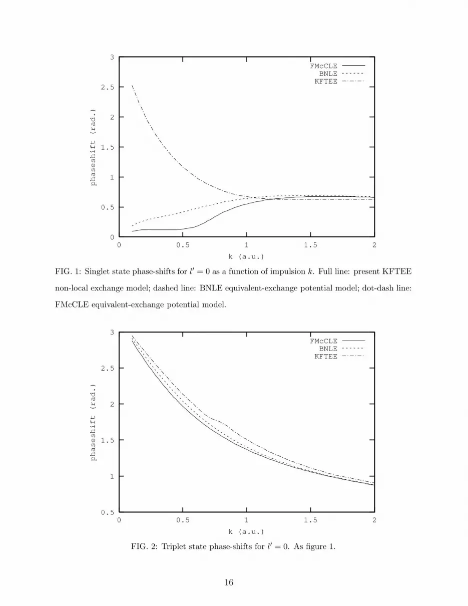
Finally, in figures 1 to 4, we compare, for the lowest two partial waves, the phaseshifts

obtained using the KFTEE code with those from the local equivalent-exchange potential

models FMcCLE and BNLE. Important differences are found up to k ≈ 1.1 a.u. (15 eV

energy). In the case of singlet spin states, for l′ = 0 (figure 1) the equivalent-exchange

models give severe underestimates but for l′ = 1 (figure 3) they are acceptble. In the case

of triplet spin states, for l′ = 0 (figure 2) results are quite good but for l′ = 1 the BNLE

model gives a severe overestimate. For higher partial waves equivalent-exchange models

give fairly satisfactory results. Since Distorted Wave Born collision calculations near to

threshold converge with only about five partial waves, we would hesitate then to use a local

equivalent-exchange potential.

V. CONCLUSIONS AND PROSPECTS

We have shown that a distorted wave code, with exact treatment of exchange but using

Numerov integration, breaks down through numerical instabilities at energies below about

5 eV. We have also shown that codes with local equivalent-exchange potentiels give poor

results for low partial waves at energies below 15 eV. We propose an alternative method treat-

ing exchange exactly but using the Canonical Function technique to integrate the coupled

equations. This we believe to be numerically stable even at extremely small energies. The

present work is the first step towards a general code applicable to target atoms or molecules

in any angular momentum state and capable of using numerically generated potentials. An

alternative code is under development in which solutions are obtained by Runge-Kutta in-

tegration on a regular grid out to a radius where exchange terms are negligible; phase-shifts

are obtained by comparison with the Klapisch-Robaux iterative JWKB code [1]. In this

15

0

0.5

1

1.5

2

2.5

3

0 0.5 1 1.5 2

phaseshift (rad.)

k (a.u.)

FMcCLEBNLEKFTEE

FIG. 1: Singlet state phase-shifts for l′ = 0 as a function of impulsion k. Full line: present KFTEE

non-local exchange model; dashed line: BNLE equivalent-exchange potential model; dot-dash line:

FMcCLE equivalent-exchange potential model.

0.5

1

1.5

2

2.5

3

0 0.5 1 1.5 2

phaseshift (rad.)

k (a.u.)

FMcCLEBNLEKFTEE

FIG. 2: Triplet state phase-shifts for l′ = 0. As figure 1.

16

-0.05

0

0.05

0.1

0.15

0.2

0.25

0 0.5 1 1.5 2

phaseshift (rad.)

k (a.u.)

FMcCLEBNLEKFTEE

FIG. 3: Singlet state phase-shifts for l′ = 1. As figure 1.

0

0.5

1

1.5

2

2.5

3

3.5

0 0.5 1 1.5 2

phaseshift (rad.)

k (a.u.)

FMcCLEBNLEKFTEE

FIG. 4: Triplet state phase-shifts for l′ = 1. As figure 1.

17

code we have on the one hand f1(r) and f ′

1(r) and on the other a phase function, its deriva-

tive and a slowly-varying amplitude function for which we can safely generate the derivative

numerically. So we can get tan δl′ using a single mesh point, but without the need to carry

numerical integration of the coupled equations out to a radius (very big for small k) where

the asymptotic behaviour is given by sl′(kr) and cl′(kr) . The new code will give us the

opportunity to check the relative accuracy of phaseshift determinations using respectively

f1(r) and f ′

1(r) at one mesh-point or f1(r) at two. We also intend to test the effects at low

energy of using Bethe-Reeh type multipole polarisation potentials [6] which we will generate

numerically, for instance in the case of Na and the rare gases; this will enable us to extend

the work of Rouet et al [17]. We are particularly interested in applications to (e, 2e) and

(γ, 2e) processes involving polarised electrons.

Acknowledgments

This work was partly financed by the Lebanese University and the C.N.R.S.L. K.F. thanks

the Universite de Bretagne Occidentale for a two month stay as Professeur Invite and the

L.C.E.A. for its hospitality.

[1] Bar Shalom A 1983 Thesis University of Jerusalem

[2] Bayliss W E and Peel S J 1982 Comput. Phys. Commun. 25 7

[3] Bransden B H and Noble C J 1976 J. Phys. B: At. Mol. Opt. Phys. 9 1507

[4] Bray I 1994 Phys. Rev. Lett. 73 1088

[5] Burgess A 1963 Proc. Phys. Soc. 81 442

[6] Drachman R J and Temkin A 1972 Case Studies in Atomic Physics II, ed. E W McDaniel

and M R C McDowell, North Holland, 399

[7] Fakhreddine K and Kobeissi H 1994 Int. J. Quantum Chem. 49 773

[8] Fakhreddine K, Kobeissi H and Korec M 1999 Int. J. Quantum Chem. 73 325

[9] Furness J B and McCarthy I E 1973 J. Phys. B: At. Mol. Opt. Phys. 6 2280

[10] Kobeissi H and Kobeissi M 1988 J. Comput. Phys. 77 501

[11] Kobeissi H Fakhreddine K and Kobeissi M 1991 Int. J. Quantum Chem. XL 11

18

[12] Kobeissi H and Fakhreddine K 1991a J. Phys. II (France) 1 899

[13] Kobeissi H and Fakhreddine K 1991b J. Comput. Phys. 95 505

[14] Numerov B 1933 Obser. Cent. Astrophys. (Russ.) 2 188

[15] McDowell M R C, Morgan L and Myerscough V P 1974a Comput. Phys. Commun. 7 38

[16] McDowell M R C, Myerscough V P and Morgan L 1974b J. Phys. B: At. Mol. Opt. Phys. 24

657

[17] Rouet F, Tweed R J and Langlois J 1996 J. Phys. B: At. Mol. Opt. Phys. 29 1767

[18] Scott T and McDowell M R C 1975 J. Phys. B: At. Mol. Opt. Phys. 8 1851

19