Seediscussions,stats,andauthorprofilesforthispublicationat:https://www.researchgate.net/publication/223076393

Distribution,abundance,andpredationeffectsofepipelagicctenophoresandjellyfishinthewesternArcticOcean

ArticleinDeepSeaResearchPartIITopicalStudiesinOceanography·July2010

DOI:10.1016/j.dsr2.2009.08.011

CITATIONS

25

READS

67

4authors,including:

JenniferE.Purcell

WesternWashingtonUniversity

153PUBLICATIONS6,814CITATIONS

SEEPROFILE

KseniaN.Kosobokova

P.P.ShirshovInstituteofOceanology

85PUBLICATIONS1,437CITATIONS

SEEPROFILE

TerryE.Whitledge

UniversityofAlaskaFairbanks

121PUBLICATIONS5,645CITATIONS

SEEPROFILE

AllcontentfollowingthispagewasuploadedbyKseniaN.Kosobokovaon30November2016.

Theuserhasrequestedenhancementofthedownloadedfile.Allin-textreferencesunderlinedinblue

arelinkedtopublicationsonResearchGate,lettingyouaccessandreadthemimmediately.

ARTICLE IN PRESS

Deep-Sea Research II 57 (2010) 127–135

Contents lists available at ScienceDirect

Deep-Sea Research II

0967-06

doi:10.1

� Corr

E-m

journal homepage: www.elsevier.com/locate/dsr2

Distribution, abundance, and predation effects of epipelagic ctenophores andjellyfish in the western Arctic Ocean

Jennifer E. Purcell a,�, Russell R. Hopcroft b, Ksenia N. Kosobokova c, Terry E. Whitledge b

a Western Washington University, Shannon Point Marine Center, 1900 Shannon Point Rd, Anacortes, WA 98221, USAb Institute of Marine Science, University of Alaska Fairbanks, Fairbanks, AK 99775-7220, USAc Shirshov Institute of Oceanology RAS, 36 Nakimova Avenue, 117997 Moscow, Russian Federation

a r t i c l e i n f o

Available online 13 August 2009

Keywords:

Gelatinous zooplankton

ROV

Competition

Climate change

45/$ - see front matter & 2009 Elsevier Ltd. A

016/j.dsr2.2009.08.011

esponding author. Fax: +1360 2931083.

ail address: purcelj3@wwu.edu (J.E. Purcell).

a b s t r a c t

The Arctic Ocean is undergoing changes at an unprecedented rate because of global climate change.

Especially poorly-studied in arctic waters are the gelatinous zooplankton, which are difficult to study

using traditional oceanographic methods. A distinct zooplanktivore community was characterized in

the surface 100 m by use of a Remotely Operated Vehicle, net collections, and SCUBA diving. The large

scyphomedusa, Chrysaora melanaster, was associated with the warm Pacific water at �35–75 m depth.

A diverse ctenophore community lived mainly above the C. melanaster layer, including Dryodora

glandula, a specialized predator of larvaceans, Beroe cucumis, a predator of other ctenophores, and the

extremely fragile Bolinopsis infundibulum, which was the most abundant species. Gut content analyses

showed that Mertensia ovum selectively consumed the largest copepods (Calanus spp.) and amphipods

(Parathemisto libellula); B. infundibulum consumed smaller copepods and pteropods (Limacina helicina).

Large copepods were digested by M. ovum in �12 h at �1.5 to 0 1C, but by B. infundibulum in only �4 h.

We estimated that M. ovum consumed an average of �2% d�1 of the Calanus spp. copepods and that

B. infundibulum consumed �4% d�1 of copepods o3 mm prosome length. These are significant

consumption rates given that Calanus spp. have life-cycles of 2 or more years and are eaten by

vertebrates including bowhead whales and arctic cod.

& 2009 Elsevier Ltd. All rights reserved.

1. Introduction

Little is known about the ctenophores, siphonophores, hydro-medusae, and scyphomedusae in polar seas (Pag�es, 1997). Basicdescriptions of gelatinous zooplankton from the Arctic Ocean arewidely scattered in the published literature over the past century(e.g., Bigelow, 1920; Stepanjants, 1989; Sirenko, 2001), but thesegenerally provide only information on their occurrence, withoutinformation on their abundance or ecology. One of the fewexceptions shows gelatinous species to be relatively abundantthroughout the water column (Raskoff et al., 2005).

The above gelatinous taxa are predators, whose feeding onzooplankton, such as the abundant copepods (Smith and Schnack-Schiel, 1990; Conover and Huntley, 1991; Mumm et al., 1998;Hopcroft et al., 2005), generally is of unknown importance in theArctic. Only a few studies consider the trophic importance ofcarnivorous gelatinous species in Arctic surface waters. In theeastern Arctic, the ctenophore, Mertensia ovum, is a predominantgelatinous species year-round (Percy, 1989; Swanberg and

ll rights reserved.

Bamstedt, 1991a, b; Siferd and Conover, 1992; Lundberg et al.,2006). These ctenophores were estimated to consume up to9% d�1 of the populations of the larger copepods (Calanus glacialis)and 3–4% d�1 of the smaller copepod species (Siferd and Conover,1992). Other under-studied gelatinous predators may have similarecological importance (e.g., Hosia and Bamstedt, 2007). Bolinopsis

spp. ctenophores are widely distributed but little-studied becauseof their fragile construction (exceptions are Kremer et al., 1986;Kasuya et al., 1994; Kinoshita et al., 2006). They are reported fromboreal waters (Siferd and Conover, 1992; Raskoff et al., 2005;Hosia and Bamstedt, 2007), but their importance as predators isunknown.

The Arctic Ocean has strong near-surface discontinuities oftemperature and salinity and deeper distinct water masses ofdifferent origin layered throughout the water column. The mainlayers include a thin, low-salinity layer immediately below the ice(o10 m depth), then a mixed layer (o40 m) followed by a layeroriginating from the Bering Strait and West-Wind Ridge (�40–200 m), the Atlantic waters entering the Arctic through Fram Strait(350–600 m), and waters of uniquely Arctic character below600 m (McLaughlin et al., 2005). The vertical distributions ofgelatinous zooplankton are known to be related to the physicalstructure in the water column. Numerous examples exist of

ARTICLE IN PRESS

J.E. Purcell et al. / Deep-Sea Research II 57 (2010) 127–135128

horizontal layers of gelatinous species at halo- or thermoclines(reviewed in Graham et al., 2001; see also Rakow and Graham,2006).

An Arctic Ocean cruise in 2002 showed pronounced layering ofthe gelatinous taxa among those water layers with a distinctdiscontinuity between shallow-living (o100 m) and deep-living(4200 m) species (Raskoff et al., 2005). The focus of the presentstudy is to quantify the shallow gelatinous community andestimate their trophic importance in this ecosystem.

2. Materials and methods

2.1. Study area

The data were collected during the NOAA Ocean Explorationcruise HLY0502 29 from 29 June to 23 July, 2005 aboard the U.S.Coast Guard Cutter Healy, a zone 6 ice breaker, at 12 stations inthe Canada Basin (Table 1). The ship track constituted a primarilynorthwesterly loop from Barrow, Alaska in the south to 75.51N,�162.11W in the north. For station locations relative tobathymetry, see Fig. 1 in Raskoff et al. (2010). The stations wereconducted in areas with small leads of open water within the icecover.

2.2. Measurements of the physical structure of the upper 100-m

water column

Temperature, salinity, and fluorescence versus depth data werecollected in the upper 100 m in the water column with a CTDinstrument. The primary casts from the vessel were obtained witha Sea Bird model 911Plus CTD with integrated dissolved oxygen(SBE-43), fluorescence (Chelsea Aquatrack A), and transmiss-ometer (Wet Labs Cstar) sensors combined with a Sea Bird 12-bottle rosette carousel. The CTD downcasts were taken at20 m min�1 in the upper 75 m and increasing to 60 m min�1

thereafter. In order to collect physical measurement withoutinfluence from the vessel, a shallow CTD instrument (SBE19+)equipped with fluorescence sensors was deployed to 100 m atmost stations through 20 cm ice core holes. The coring stationswere located approximately 100 m from the vessel and theinstrument package was lowered at o10 m min�1 in the upper20 m and thereafter increased to 15 m min�1. Fluorescence wasused to indicate chlorophyll-phytoplankton biomass in the watercolumn.

2.3. Distribution and abundance of ctenophores, jellyfish, and

zooplankton

The study utilized the Remotely Operated Vehicle (ROV) Global

Explorer (Deep Sea Systems), a 3000-m-rated submersible with a720P High Definition (HDTV) video system. A Sea Bird CTD wasattached to the ROV for collection of oceanographic data duringthe dives. On each dive, the entire water column was traversedvertically to ascertain the distribution of gelatinous animals. TheROV was lowered and raised at a rate of �2 m s�1 in the upperwater column; therefore, only conspicuous gelatinous animalscould be counted. Real-time sightings were annotated with timeand depth, and tabulated post-dive.

Gelatinous zooplankton was collected with a 800-mm soft-mesh plankton net with a bag cod-end and slow-flow GeneralOceanics flowmeter. The net was deployed in ice-free areas for10 min at 5, 10, 15, 20, 25, and 30 m depths, and fished horizontallybecause of the drift of the ship. The living specimens were

identified, counted, and volumes measured in a graduatedcylinder immediately after collection.

Sizes of the cydippid ctenophore, Mertensia ovum, wereevaluated by the method of Purcell (1988). The oral–aboralstomodeum length and tentacle-bulb lengths were measuredwith a ruler under magnification from a dissecting microscope onsubmerged, living, diver-collected ctenophores. The live displace-ment volumes of these specimens were measured with graduatedcylinders. The specimens then were preserved individually in 5%formalin–seawater solution, and the lengths of isolated, preservedtentacle-bulbs measured as above. The relationships of tentacle-bulb length to ctenophore length and volume were determined bylogarithmic regression.

Mesozooplankton throughout the water column were collectedusing a Hydrobios Midi Multinet (0.25 m2 mouth, 150-mm mesh)hauled from the bottom (to a maximum of 3000 m) to the surfaceat �0.5 m s–1 (see Kosobokova and Hopcroft, 2010). Only datafrom the upper 3 strata (0–24, 25–49, and 50–100 m) for prey ofM. ovum are reported here. Samples were preserved in 4%formalin/seawater for later processing. All mesozooplanktonorganisms 41 mm in the samples were counted and measuredwith the aid of a dissecting microscope. For the plankton o1 mm,a 1/10th to 1/8th sub-sample was taken with a stempel-pipetteand all organisms counted. Most taxa were identified to species.Copepodite stages of calanoid copepods were counted separately.Prosome length (PL) was used to distinguish early copepoditestages CI–CIII of Calanus, which belonged exclusively to Calanus

glacialis and C. hyperboreus.Only prey taxa (copepods and amphipods) of ctenophore

species collected for gut analysis were included in this analysis.Copepods were assigned to 4 size groups, 45, 3–5, 1.5–2.9, ando1.5 mm PL based on the mean size at stage typical for species inthis region. The number of zooplankton m�2 was calculated foreach station as the sum of copepods and amphipods m�3 inzooplankton samples from 0 to 24, 25 to 49, and 50 to 100 m-depth intervals, each multiplied by the respective depth. Theweighted mean depth (WMD) of copepods and amphipods at eachstation was calculated as

P(nizidi)/

P(nizi), where di is the

midpoint of the sample depth-interval, zi is the thickness of thestratum, and ni is the number of individuals m�3 within depthlayer i.

2.4. Predation by ctenophores

Ctenophores (Mertensia ovum and Bolinopsis infundibulum) forgut content analysis were collected in jars by SCUBA divers at10–25 m depth. The specimens were immediately preserved insmall individual jars with 5% formalin–seawater solution whenthe divers returned to the surface, thereby minimizing furtherdigestion of the prey. All zooplankton in the samples wereidentified to general taxon and counted. Because digested preyoften could not be identified to species, calanoid copepods wereassigned to 4 size groups, 45, 3–5, 1.5–2.9, and o1.5 mm PL. Thepreserved tentacle bulbs of M. ovum were isolated from attachedtissue and measured in order to estimate the sizes of the livingctenophores (Purcell, 1988), as above. Prey selection indices werecalculated according to Pearre (1982).

In order to estimate predation rates from gut content analyses,digestion times of the prey organisms must be determined (e.g.,Purcell, 1997). Diver-collected ctenophores were retained in their1-L collecting jars in order to minimize disturbance, maintained ina walk-in cold room at ambient temperature (�1.0 to 0 1C), andallowed to clear their field gut contents. Calanus spp. copepodswere collected from the surface 20 m in vertical tows made with a1.0-m-diameter, 800-mm-mesh plankton net with a bag cod-end.

ARTIC

LEIN

PRESS

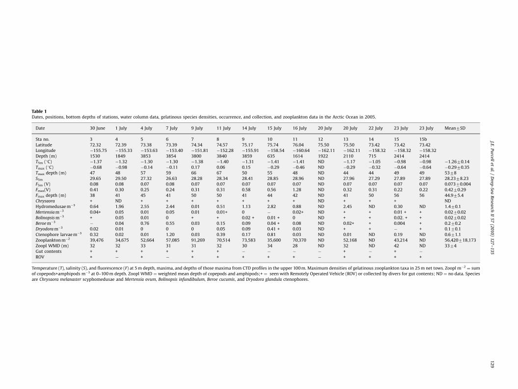
Table 1Dates, positions, bottom depths of stations, water column data, gelatinous species densities, occurrence, and collection, and zooplankton data in the Arctic Ocean in 2005.

Date 30 June 1 July 4 July 7 July 9 July 11 July 14 July 15 July 16 July 20 July 20 July 22 July 23 July 23 July Mean7SD

Sta no. 3 4 5 6 7 8 9 10 11 12 13 14 15 15b

Latitude 72.32 72.39 73.38 73.39 74.34 74.57 75.17 75.74 76.04 75.50 75.50 73.42 73.42 73.42

Longitude �155.75 �155.33 �153.63 �153.40 �151.81 �152.28 �155.91 �158.54 �160.64 �162.11 �162.11 �158.32 �158.32 �158.32

Depth (m) 1530 1849 3853 3854 3800 3840 3859 635 1614 1922 2110 715 2414 2414

T5m (1C) �1.37 �1.32 �1.30 �1.30 �1.38 �1.40 �1.31 �1.41 �1.41 ND �1.17 �1.05 �0.98 �0.98 �1.2670.14

Tmax (1C) �0.68 �0.98 �0.14 �0.11 0.17 0.06 0.15 �0.29 �0.46 ND �0.29 �0.32 �0.64 �0.64 �0.2970.35

Tmax depth (m) 47 48 57 59 66 67 50 55 48 ND 44 44 49 49 5378

S5m 29.65 29.50 27.32 26.63 28.28 28.34 28.41 28.85 28.96 ND 27.96 27.29 27.89 27.89 28.2378.23

F5m (V) 0.08 0.08 0.07 0.08 0.07 0.07 0.07 0.07 0.07 ND 0.07 0.07 0.07 0.07 0.07370.004

Fmax(V) 0.41 0.30 0.25 0.24 0.31 0.31 0.58 0.56 1.28 ND 0.32 0.31 0.22 0.22 0.4270.29

Fmax depth (m) 38 41 45 41 50 50 41 44 42 ND 41 50 56 56 44.975.4

Chrysaora + ND + + + + + + + ND + + + ND

Hydromedusae m�3 0.64 1.96 2.55 2.44 0.01 0.51 1.13 2.82 0.88 ND 2.45 ND 0.30 ND 1.470.1

Mertensia m�3 0.04+ 0.05 0.01 0.05 0.01 0.01+ 0 � 0.02+ ND + + 0.01 + + 0.0270.02

Bolinopsis m�3 + 0.05 0.01 0 + + 0.02 + 0.01 + 0 ND + + 0.02. + + 0.0270.02

Beroe m�3� 0.04 0.76 0.55 0.03 0.15 0.09 0.04 + 0.08 ND 0.02+ + 0.004 + 0.270.2

Dryodora m�3 0.02 0.01 0 0 0 0.05 0.09 0.41 + 0.03 ND + + � + 0.170.1

Ctenophore larvae m�3 0.32 0.02 0.01 1.20 0.03 0.39 0.17 0.81 0.03 ND 0.01 ND 0.19 ND 0.671.1

Zooplankton m�2 39,476 34,675 52,664 57,085 91,269 70,514 73,583 35,600 70,370 ND 52,168 ND 43,214 ND 56,420718,173

Zoopl WMD (m) 32 32 33 31 31 32 30 34 28 ND 32 ND 42 ND 3374

Gut contents + + + + + + � � � � + � + �

ROV + � + � + + + + + � + + + +

Temperature (T), salinity (S), and fluorescence (F) at 5 m depth, maxima, and depths of those maxima from CTD profiles in the upper 100 m. Maximum densities of gelatinous zooplankton taxa in 25 m net tows. Zoopl m�2¼ sum

of copepods+amphipods m�3 at 0–100 m depth. Zoopl WMD ¼ weighted mean depth of copepods and amphipods;+ ¼ seen with Remotely Operated Vehicle (ROV) or collected by divers for gut contents; ND ¼ no data. Species

are Chrysaora melanaster scyphomedusae and Mertensia ovum, Bolinopsis infundibulum, Beroe cucumis, and Dryodora glandula ctenophores.

J.E.

Pu

rcellet

al.

/D

eep-Sea

Resea

rchII

57

(20

10

)1

27

–13

51

29

ARTICLE IN PRESS

J.E. Purcell et al. / Deep-Sea Research II 57 (2010) 127–135130

Individual copepods were released undamaged into the jars, andthe time of capture by the ctenophore documented. Thectenophores with prey were checked at hourly intervals and theappearance of the prey noted. The time when the digested preywas no longer visible to the naked eye equaled the digestion time.After this time, a new copepod was released in each jar and theprocess repeated for 1–2 d. After the last measurement, eachctenophore was preserved to check for remaining gut contentswith a dissecting microscope.

An alternative method to estimate digestion times of prey usedctenophores collected on one dive, 6 of which were preservedimmediately for initial gut contents. Three ctenophores werepreserved at 3-h intervals thereafter. Gut content analyses wereconducted as for other field-collected specimens. The minimumdigestion time equaled the interval when no ingested prey wasidentifiable with magnification of a dissecting microscope.

Because we had ctenophore density estimates only above 30 mdepth, predation rates were calculated only for zooplanktonsamples from 0 to 24 m. Daily predation rates by Mertensia ovum

and Bolinopsis infundibulum were estimated from the numbers ofcopepods in each size-group eaten at each station, divided by thedigestion times, and multiplied by the 24 h d�1. The percentages ofthe copepod populations eaten per day at each station wereestimated by multiplying these individual rates by the ctenophoredensity and dividing by the densities of zooplankton in each group.

3. Results

3.1. Physical structure of the upper 100 m

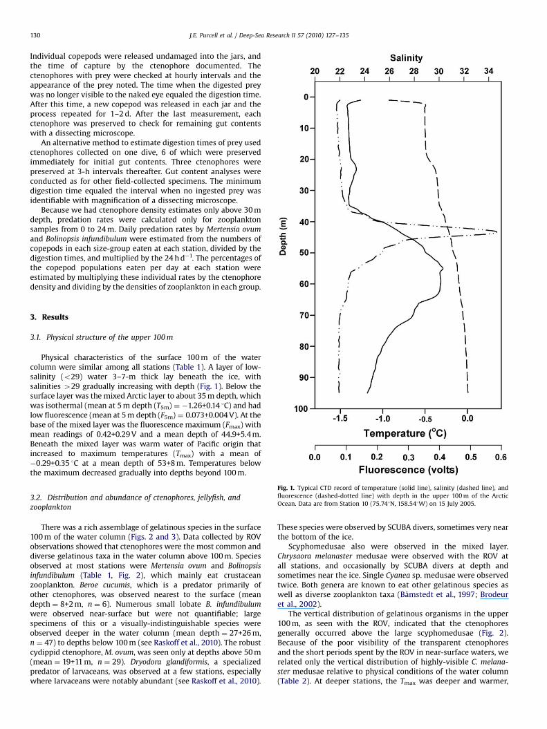
Physical characteristics of the surface 100 m of the watercolumn were similar among all stations (Table 1). A layer of low-salinity (o29) water 3–7-m thick lay beneath the ice, withsalinities 429 gradually increasing with depth (Fig. 1). Below thesurface layer was the mixed Arctic layer to about 35 m depth, whichwas isothermal (mean at 5 m depth (T5m) ¼ �1.26+0.14 1C) and hadlow fluorescence (mean at 5 m depth (F5m) ¼ 0.073+0.004 V). At thebase of the mixed layer was the fluorescence maximum (Fmax) withmean readings of 0.42+0.29 V and a mean depth of 44.9+5.4 m.Beneath the mixed layer was warm water of Pacific origin thatincreased to maximum temperatures (Tmax) with a mean of�0.29+0.35 1C at a mean depth of 53+8 m. Temperatures belowthe maximum decreased gradually into depths beyond 100 m.

Fig. 1. Typical CTD record of temperature (solid line), salinity (dashed line), and

fluorescence (dashed-dotted line) with depth in the upper 100 m of the Arctic

Ocean. Data are from Station 10 (75.741N, 158.541W) on 15 July 2005.

3.2. Distribution and abundance of ctenophores, jellyfish, and

zooplankton

There was a rich assemblage of gelatinous species in the surface100 m of the water column (Figs. 2 and 3). Data collected by ROVobservations showed that ctenophores were the most common anddiverse gelatinous taxa in the water column above 100 m. Speciesobserved at most stations were Mertensia ovum and Bolinopsis

infundibulum (Table 1, Fig. 2), which mainly eat crustaceanzooplankton. Beroe cucumis, which is a predator primarily ofother ctenophores, was observed nearest to the surface (meandepth ¼ 8+2 m, n ¼ 6). Numerous small lobate B. infundibulum

were observed near-surface but were not quantifiable; largespecimens of this or a visually-indistinguishable species wereobserved deeper in the water column (mean depth ¼ 27+26 m,n ¼ 47) to depths below 100 m (see Raskoff et al., 2010). The robustcydippid ctenophore, M. ovum, was seen only at depths above 50 m(mean ¼ 19+11 m, n ¼ 29). Dryodora glandiformis, a specializedpredator of larvaceans, was observed at a few stations, especiallywhere larvaceans were notably abundant (see Raskoff et al., 2010).

These species were observed by SCUBA divers, sometimes very nearthe bottom of the ice.

Scyphomedusae also were observed in the mixed layer.Chrysaora melanaster medusae were observed with the ROV atall stations, and occasionally by SCUBA divers at depth andsometimes near the ice. Single Cyanea sp. medusae were observedtwice. Both genera are known to eat other gelatinous species aswell as diverse zooplankton taxa (Bamstedt et al., 1997; Brodeuret al., 2002).

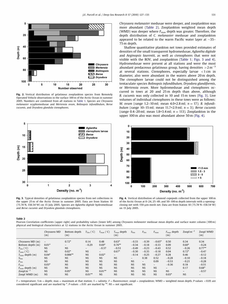
The vertical distribution of gelatinous organisms in the upper100 m, as seen with the ROV, indicated that the ctenophoresgenerally occurred above the large scyphomedusae (Fig. 2).Because of the poor visibility of the transparent ctenophoresand the short periods spent by the ROV in near-surface waters, werelated only the vertical distribution of highly-visible C. melana-

ster medusae relative to physical conditions of the water column(Table 2). At deeper stations, the Tmax was deeper and warmer,

ARTICLE IN PRESS

Table 2Pearson Correlation coefficients (upper right) and probability values (lower left) amon

physical and biological characteristics at 12 stations in the Arctic Ocean in summer 20

Chrysaora MD

(m)

Bottom depth

(m)

T5m (1C) Tmax (1C) Tmax

(m)

Chrysaora MD (m) – 0.72n 0.14 0.48 0.63

Bottom depth (m) 0.01n – �0.29 0.69n 0.76

T5m (1C) NS NS – �0.37 �0.5

Tmax (1C) NS 0.02n NS – 0.67

Tmax depth (m) 0.04n 0.006nn NS 0.02n –

S5m NS NS NS NS NS

F5m NS NS NS NS NS

Fmax 0.03n NS NS NS NS

Fmax depth (m) NS NS NS NS NS

Zoopl m�2 NS 0.05n NS 0.01nn NS

Zoopl WMD (m) NS NS 0.01nn NS NS

T ¼ temperature; 5 m ¼ depth; max ¼ maximum at that station; S ¼ salinity; F ¼ fluor

considered significant and are marked by n. P-values o0.01 are marked by nn. NS ¼ not

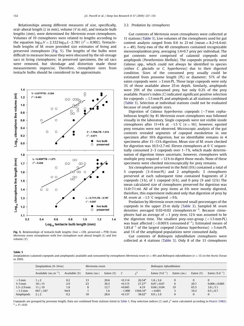
Fig. 3. Typical densities of gelatinous zooplankton species from net collections in

the upper 25 m of the Arctic Ocean in summer 2005. Data are from Station 10

(75.741N, 158.541W) on 15 July 2005. Species are Aglantha digitale hydromedusae

and Beroe cucumis and Dryodora glandula ctenophores.

Fig. 2. Vertical distribution of gelatinous zooplankton species from Remotely

Operated Vehicle observations in the surface 100 m of the Arctic Ocean in summer

2005. Numbers are combined from all stations in Table 1. Species are Chrysaora

melanaster scyphomedusae and Mertensia ovum, Bolinopsis infundibulum, Beroe

cucumis, and Dryodora glandula ctenophores.

J.E. Purcell et al. / Deep-Sea Research II 57 (2010) 127–135 131

Chrysaora melanaster medusae were deeper, and zooplankton wasmore abundant (Table 2). Zooplankton weighted mean depth(WMD) was deeper where Fmax depth was greater. Therefore, thedepth distribution of C. melanaster medusae and zooplanktonappeared to be related to the warm Pacific water layer at �35–75 m depth.

Shallow quantitative plankton net tows provided estimates ofdensities of the small transparent hydromedusae, Aglantha digitale

and Aeginopsis laurentii, as well as ctenophores that were notvisible with the ROV, and zooplankton (Table 1; Figs. 3 and 4).Hydromedusae were present at all stations and were the mostabundant predaceous gelatinous group, having densities 42 m�3

at several stations. Ctenophores, especially larvae o1 cm indiameter, also were abundant in the waters above 20 m depth.The ctenophore larvae could not be distinguished among thetentaculate species Bolinopsis infundibulum, Dryodora glandiformis,or Mertensia ovum. More hydromedusae and ctenophores oc-curred in tows at 20 and 25 m depth than above, althoughB. cucumis was only collected in 10 and 15 m tows (Fig. 3). Livevolumes of individual ctenophores in these tows were as follows:M. ovum (range 1.2–10 ml; mean 4.0+2.8 ml; n ¼ 17); B. infundi-

bulum (range 10–15 ml; mean 11.7+2.9 ml; n ¼ 3); Beroe cucumis

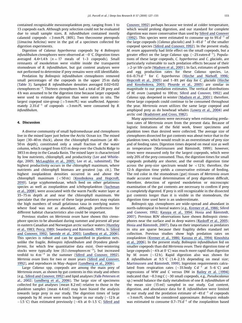
(range 0.4–20 ml; mean 1.8+3.4 ml; n ¼ 113). Zooplankton in theupper 100 m also was most abundant above 50 m (Fig. 4).

g Chrysaora melanaster medusae mean depths and surface water column (100 m)

05.

depth S5m F5m Fmax Fmax depth

(m)

Zoopl m�2 Zoopl WMD

(m)

n�0.33 �0.39 �0.65n 0.50 0.34 0.34

nn�0.34 �0.18 �0.33 0.09 0.60n

�0.24

3 �0.49 �0.23 �0.43 0.52 �0.26 0.77nn

n�0.30 �0.35 �0.18 0.04 0.72n

�0.47

�0.14 �0.25 �0.27 0.28 0.46 �0.12

– 0.38 0.52 �0.28 �0.10 �0.18

NS – 0.09 �0.53 �0.21 �0.28

NS NS – �0.36 0.18 �0.51

NS NS NS – 0.17 0.68n

NS NS NS NS – �0.57

NS NS NS 0.03n NS –

escence; zoopl ¼ zooplankton; WMD ¼ weighted mean depth. P-values o0.05 are

significant.

Fig. 4. Vertical distribution of calanoid copepods collected from the upper 100 m

of the Arctic Ocean at 0–24, 25–49, and 50–100 m depth intervals with a opening-

closing net with 150-mm-mesh net. Data are from Station 10 (75.741N–158.541W)

on 15 July 2005.

ARTICLE IN PRESS

J.E. Purcell et al. / Deep-Sea Research II 57 (2010) 127–135132

Relationships among different measures of size, specifically,oral–aboral length (L in mm), volume (V in ml), and tentacle-bulblengths (mm), were determined for Mertensia ovum ctenophores.Volumes of 19 ctenophores were related to lengths according tothe equation log10 V ¼ 2.332 log10 L�2.781 (r2

¼ 0.902). Tentacle-bulb lengths of M. ovum provided size estimates of living andpreserved ctenophores (Fig. 5). The lengths of the bulbs weredifficult to measure because they were obscured by the oil-storagesacs in living ctenophores; in preserved specimens, the oil sacswere removed, but shrinkage and distortion made thosemeasurements imprecise. Therefore, ctenophore sizes fromtentacle bulbs should be considered to be approximate.

Table 3Zooplankton (calanoid copepods and amphipods) available and consumed by ctenophor

in 2005.

Zooplankton (0–24 m) Mertensia ovum

Available (no. m�3) Available (%) Eaten (no.) Eaten (%) C

45 mm 172 0.2 13 20.6 +0

3–5 mm 18715 2.9 23 36.5 +0

1.5–2.9 mm 11710 1.8 8 12.7 +0

o1.5 mm 6677347 94.9 1 1.6 �

Amphipods 272 0.2 18 28.6 +0

Copepods are grouped by prosome length. Data are combined from stations listed in Tan¼ Po0.01

Fig. 5. Relationships of tentacle-bulb lengths (live ¼ LTB, preserved ¼ PTB) from

Mertensia ovum ctenophores with live ctenophore oral–aboral length (L) and live

volume (V).

3.3. Predation by ctenophores

Gut contents of Mertensia ovum ctenophores were collected at11 stations (Table 3). Live volumes of the ctenophores used for gutcontent analysis ranged from 0.6 to 21 ml (mean ¼ 8.2+4.4 ml;n ¼ 49). Forty-two of the 49 ctenophores contained recognizablemesozooplankton prey, averaging 1.4+0.7 prey per individual. Thegut contents were comprised of calanoid copepods andamphipods (Parathemisto libellula). The copepods primarily wereCalanus spp., which could not always be identified to species(either C. glacialis or C. hyperboreus) due to their digestedcondition. Sizes of the consumed prey usually could beestimated from prosome length (PL) or diameter; 57% of theeaten copepods were 43 mm PL. Those large copepods were only3% of those available above 25 m depth. Similarly, amphipodswere 29% of the consumed prey, but only 0.2% of the preyavailable. Pearre’s index (C) indicated significant positive selectionfor copepods 41.5 mm PL and amphipods at all stations combined(Table 3). Selection at individual stations could not be evaluatedbecause of small sample sizes.

Digestion of Calanus hyperboreus copepods (�7 mm cepha-lothorax length) by 41 Mertensia ovum ctenophores was followedvisually in the laboratory. Single copepods were not visible insidectenophores after 11+4 h at �1.5 1C (n ¼ 16); however, egestedprey remains were not observed. Microscopic analysis of the gutcontents revealed segments of copepod exoskeleton in onespecimen after 10 h digestion, but no identifiable remains in 4specimens after 11–13 h digestion. Mean size of M. ovum checkedfor digestion was 10.5+2.7 ml. Eleven ctenophores at 0 1C sequen-tially consumed 2–3 copepods over 1–7 h, which made determi-nation of digestion times uncertain; however, ctenophores withmultiple prey required 412 h to digest those meals. None of thesespecimens were checked microscopically for prey remains.

Six ctenophores preserved in the field (0 h) contained a total of5 copepods (3–6 mm PL) and 2 amphipods; 3 ctenophorespreserved at each subsequent time contained fragments of 2copepods (3 h), of 1 copepod (6 h), and 0 prey (9 and 12 h) Themean calculated size of ctenophores preserved for digestion was11.0+7.1 ml. All of the prey items at 0 h were mostly digested,therefore, this experiment indicated only that digestion of prey byM. ovum at �1.5 1C required 49 h.

Predation by Mertensia ovum removed small percentages of thecopepods in the upper 25 m daily (Table 3). Sampled M. ovum

densities averaged 0.02+0.02 ctenophores m�3. Because cteno-phores had an average of 41 prey item, 12 h was assumed to bethe digestion time. The smallest prey-size-group (o1.5 mm PL)was least affected (o0.001% consumed d�1). Estimated means of1.8% d�1 of the largest copepod (Calanus hyperboreus) 45 mm PLand 1% of the amphipod populations were consumed daily.

Gut contents of Bolinopsis infundibulum ctenophores werecollected at 4 stations (Table 3). Only 8 of the 13 ctenophores

es Mertensia ovum (n ¼ 49) and Bolinopsis infundibulum (n ¼ 13) in the Arctic Ocean

Bolinopsis infundibulum

w2 Eaten (% d�1) Eaten (no.) Eaten (%) Eaten (% d�1)

.114 26.54n 1.873.6 0 0 0

.115 27.27n 0.0770.07 6 20.7 0.00670.005

.045 4.19 0.0470.04 19 65.5 3.875.1

1.000 1504.16n {0.001 3 10.3 0.570.7

.137 38.62n 0.971.0 0 0 0

ble 1. Prey selection indices (C) and w2 were calculated according to Pearre (1982).

ARTICLE IN PRESS

J.E. Purcell et al. / Deep-Sea Research II 57 (2010) 127–135 133

contained recognizable mesozooplankton prey, ranging from 1 to13 copepods each. Although prey selection could not be evaluateddue to small sample sizes, B. infundibulum contained mostlycalanoid copepods o3 mm PL (80%). Two thecosome pteropods(Limacina helicina) were in the gut of a specimen collected fordigestion experiments.

Digestion of Calanus hyperboreus copepods by 4 Bolinopsis

infundibulum ctenophores were observed at �0 1C. Digestion timesaveraged 4.4+1.4 h (n ¼ 17 meals of 1–3 copepods). Smallremnants of exoskeleton were visible inside the transparentstomodeum of B. infundibulum, but gut content analyses werenot performed to determine if prey remains were still identifiable.

Predation by Bolinopsis infundibulum ctenophores removedsmall percentages of the copepods in the upper 25 m daily(Table 3). Sampled B. infundibulum densities averaged 0.02+0.02ctenophores m�3. Thirteen ctenophores had a total of 28 prey and4 h was assumed to be the digestion time because larger copepodswere used to estimate digestion than were eaten in situ. Thelargest copepod size-group (45 mm PL) was unaffected. Approxi-mately 2.3% d�1 of copepods o3 mm PL were consumed by B.

infundibulum.

4. Discussion

A diverse community of small hydromedusae and ctenophoreslive in the mixed layer just below the Arctic Ocean ice. The mixedlayer (30–40 m thick), above the chlorophyll maximum (at 40–50 m depth), constituted only a small fraction of the watercolumn, which ranged from 635 m deep over the Chukchi Ridge to3853 m deep in the Canada Basin. The mixed layer is characterizedby low nutrients, chlorophyll, and productivity (Lee and Whitle-dge, 2005; McLaughlin et al., 2005; Lee et al., submitted). Thehighest productivity occurs in the chlorophyll maximum, wherenutrients and chlorophyll biomass are greatest (op. cit.). Thehighest zooplankton densities occurred in and above thechlorophyll maximum (o50 m) (Kosobokova and Hopcroft,2010). Large scyphomedusae, which feed on other gelatinousspecies as well as zooplankton and ichthyoplankton (Suchmanet al., 2008), were associated with the warm Pacific water layer at35–75 m depth at and near the chlorophyll maximum. Wespeculate that the presence of these large predators may explainthe high numbers of small gelatinous taxa in overlying waterswhere food was not as abundant, although preferences fordifferent habitat characteristics also could be important.

Previous studies on Mertensia ovum have shown this cteno-phore species to be abundant during summer and present all yearin eastern Canadian and Norwegian arctic surface waters (Huntleyet al., 1983; Percy, 1989; Swanberg and Bamstedt, 1991a, b; Siferdand Conover, 1992; Søreide et al., 2003; Lundberg et al., 2006).This species is robust and can be quantified in plankton nets,unlike the fragile, Bolinopsis infundibulum and Dryodora glandi-

formis, for which few quantitative data exist. Over-winteringstocks were typically low (0.1 ctenophores m�3), but increasedtenfold to 4 m�3 in the summer (Siferd and Conover, 1992).Mertesia ovum lives for two or more years (Siferd and Conover,1992), and reproduces in May–August (Lundberg et al., 2006).

Large Calanus spp. copepods are among the main prey ofMertensia ovum, as shown by gut contents in this study and others(e.g., Siferd and Conover, 1992) and lipid analyses (Falk-Petersen etal., 2002; Lundberg et al., 2006). The large size of specimenscollected for gut analyses (mean 8.2 ml) relative to those in theplankton samples (mean 4.4 ml) may have biased the analysistowards large prey in our study. The digestion times of largecopepods by M. ovum were much longer in our study (�12 h at�1.5 1C) than estimated previously (�4 h at 0–1.5 1C; Siferd and

Conover, 1992) perhaps because we tested at colder temperature,which would prolong digestion, and our standard for completedigestion was more conservative than used by Siferd and Conover(1992). This species were estimated to consume up to 9% d�1 ofthe large copepods (Calanus glacialis) and 3–4% d�1 of the smallercopepod species (Siferd and Conover, 1992). In the present study,M. ovum apparently had little effect on the small copepods, but agreater effect on the large Calanus spp. (�2% eaten d�1). Popula-tions of these large copepods, C. hyperboreus and C. glacialis, areparticularly vulnerable to such predation effects because of their42-yr life cycle (Madsen et al., 2001). In fact, estimates of growthand egg production rates for these Calanus species, i.e.0.6–0.7% d�1 for C. hyperboreus (Hirche and Niehoff, 1996;Hopcroft et al., 2005) and 1–8% per day for C. glacialis (Hircheand Kosobokova, 2003; Plourde et al., 2005) are similar inmagnitude to our predation estimates. The vertical distributionsof M. ovum (sampled to 100 m; Siferd and Conover, 1992) andCalanus spp. deepened in winter (Madsen et al., 2001); therefore,these large copepods could continue to be consumed throughoutthe year. Mertensia ovum utilizes the same large copepod andamphipod prey as do bowhead whales (Lowry et al., 2004) andarctic cod (Bradstreet and Cross, 1982).

Many approximations were necessary when estimating preda-tion rates of Mertensia ovum from the present data. Because oflogistic limitations of the field work, fewer specimens andplankton tows than desired were collected. The average size ofctenophores dissected for gut contents was about twice that in theplankton tows, which would result in an overestimate of prey sizeand of feeding rates. Digestion times depend on meal size as wellas temperature (Martinussen and Bamstedt, 1999); however,times were measured only for the largest copepods, which wereonly 20% of the prey consumed. Thus, the digestion times for smallcopepods probably are shorter, and the overall digestion timeacross the prey-size spectrum would be o12 h; therefore, the12-h digestion time yields a conservative estimate of feeding.The red color in the stomodeum (gut) tissues of Mertensia ovum

made accurate visual determination of prey digestion difficult,therefore, detection of egested exoskeleton or microscopicexamination of the gut contents are necessary to confirm if preyis completely digested. If prey is still recognizable in the dissectedgut contents longer than it is visible in the stomodeum, thedigestion time used here is an underestimate.

Bolinopsis spp. ctenophores are wide-spread and abundant innorth-subtropical to boreal waters (e.g., Kremer et al., 1986; Siferdand Conover, 1992; Kasuya et al., 1994; Hosia and Bamstedt,2007). Previous ROV observations have shown Bolinopsis cteno-phores near the surface and in deep waters (Raskoff et al., 2005;Hosia and Bamstedt, 2007). Data on their importance as predatorsin situ are sparse because their fragility defies standard netcollection. Previous studies show high predation rates onzooplankton (Kremer et al., 1986; Kasuya et al., 1994; Kinoshitaet al., 2006). In the present study, Bolinopsis infundibulum fed onsmaller copepods than did Mertensia ovum. Their digestion time oflarge copepods (�4 h at 0 1C) was much more rapid than digestionby M. ovum (�12 h). Rapid digestion also was shown forB. infundibulum at 9.5 1C (1.4–2.3 h depending on meal size;Martinussen and Bamstedt, 1999). Ingestion requirements calcu-lated from respiration rates (�3% body C d�1 at 5–6 1C) andregressions of WW and C versus DW in Bailey et al. (1994)indicated that �0.3 mg C (�30 small copepods, e.g., Pseudocalanus

sp.) would balance the daily metabolism of one B. infundibulum ofthe mean size (15 ml) sampled in our study. Gut content,digestion, and abundance data for B. infundibulum were limitedin our study and the predation estimate of�4% d�1 of copepodso3 mm PL should be considered approximate. Bolinopsis mikado

was estimated to consume 0.7–7% d–1 of the zooplankton based

ARTICLE IN PRESS

J.E. Purcell et al. / Deep-Sea Research II 57 (2010) 127–135134

on minimum carbon requirements at 16–21 1C (Kinoshita et al.,2006).

The association of Chrysaora melanaster with the warm Pacificwater suggests that these medusae may have been transportedthrough the Bering Strait into the Arctic Ocean. The verticaldistribution of C. melanaster in the Bering Sea (Brodeur, 1998) wassimilar to that we observed in the Arctic Ocean. This speciesincreased dramatically in the Bering Sea during the 1990s, but hasreturned to pre-bloom abundances since 2000 (Brodeur et al.,2008). Large populations of the medusae were associated withmoderate ice cover and sea surface temperatures (Brodeur et al.,2008). With continued global warming, conditions in arcticwaters may provide more suitable habitat for this species. Thesejellyfish are known to be predators of mesozooplankton, gelati-nous zooplankton, and juvenile walleye pollock (Brodeur et al.,2002); therefore, changes in scyphomedusa abundance couldhave important consequences for the food web.

Although this and other studies have focused on large or robustgelatinous species, other small species were much more numer-ous and probably are more important predators of zooplankton.Similarly, small zooplankton is important in arctic waters(Hopcroft et al., 2005; Kosobokova and Hopcroft, 2010). Totalzooplanktivores, including chaetognaths, in the upper 25 maveraged 1.2+1.4 m�3 at our stations. The holoplanktonic hydro-medusa, Aglantha digitale, is ubiquitous in cold-temperate andboreal waters. It was previously shown to be an importantpredator of mesozooplankton (72.8% of all prey, including Oithona

similis, Temora longicornis, other copepods, cladocerans, Oikopleura

spp., and bivalve larvae), as well as tintinnids and dinoflagellates(27.2% of all prey) (Pag�es et al., 1996). Densities of A. digitale in aNorwegian fjord averaged 8.8 to 57.4 medusae m�3 mostly in0–50-m depth layer (Pag�es et al., 1996). The gelatinous species,Aeginopsis laurenti, which may eat other gelatinous species as doother narcomedusae (Raskoff, 2002), and Beroe cucumis, whicheats other ctenophores, were not included here as zooplankti-vores.

Continued thinning and reduction of the arctic ice is predictedfor the foreseeable future due to global warming (I.P.C.C., 2007).Mean sea-ice thickness was less in 2005 than in 2002 (1.5 mversus 2.3 m); as a result, mean light levels under the ice differedbetween years (9.3% of the incident light at the surface in 2005versus 2.9% in 2002), and both carbon and nitrogen uptakes byphytoplankton (integrated to 35 m) differed (4- and 20-foldgreater in 2005 than in 2002, respectively; Lee et al., submitted).Therefore, further decreases in sea-ice thickness in the CanadaBasin (Nghiem et al., 2007) and increases in open water wouldincrease available light and favor phytoplankton growth, which islimited by low light (Lee and Whitledge, 2005). Higher phyto-plankton production would provide more food for the crustaceanseaten by gelatinous zooplanktivores. All of the species studiedhere would benefit from increased food. Therefore, increasedgelatinous zooplanktivore populations could be expected to resultfrom reduction in the arctic ice.

5. Conclusions

An abundant zooplanktivore community lived in the surface100 m of the Canada Basin. Ctenophores and hydromedusae weremost abundant shallower than 50 m, above the large scyphome-dusa, Chrysaora melanaster, which was associated with the warmPacific water at �35–75 m depth. Gut content analyses showedthat Mertensia ovum selectively consumed the largest copepods(Calanus spp.) and amphipods (Parathemisto libellula), whereasBolinopsis infundibulum consumed smaller copepods and ptero-pods (Limacina helicina). Digestion of large copepods was more

rapid by M. ovum than by B. infundibulum (�12 h versus 4 h). Weestimated that M. ovum consumed �2% d�1 of the Calanus spp.copepods in the surface 25 m, which is an important effect giventhe 2-yr life-cycles of these copepods; B. infundibulum wasestimated to eat 4% d�1 of copepods o3 mm prosome length.These combined predation rates are similar to the daily growthrates of the copepods on which they prey.

Acknowledgments

We thank the crew of the USCGC Healy, especially the intrepidSCUBA divers, without whom this work would not have beenpossible. We dedicate this paper to the memories of Lt. Jessica Hilland Steven Duque from the dive team, who later lost their lives ina diving accident.

Funding NOAA Ocean Exploration Hidden Ocean: Phase IIGrant no. NA05OAR4601079, plus Grant G-2394 to TEW. The workof KNK was supported by RFBR Grant no. 03-05-64871.

References

Bailey, T.G., Youngbluth, M.J., Owen, G.P., 1994. Chemical composition and oxygenconsumption rates of the ctenophore Bolinopsis infundibulum from the Gulf ofMaine. Journal of Plankton Research 16, 673–689.

Bamstedt, U., Ishii, H., Martinussen, M.B., 1997. Is the scyphomedusa Cyaneacapillata (L.) dependent on gelatinous prey for its early development?. Sarsia82, 269–273.

Bigelow, H.B., 1920. Medusae and Ctenophora. Report of the Canadian ArcticExpedition 1913–18. Southern Party 1913–1916 8, 3H–20H.

Bradstreet, S.W., Cross, W.E., 1982. Trophic relationships of high ice edges. Arctic35, 1–12.

Brodeur, R.D., 1998. In situ observations of the association between juvenile fishesand scyphomedusae in the Bering Sea. Marine Ecology Progress Series 163,11–20.

Brodeur, R.D., Decker, M.B., Ciannelli, L., Purcell, J.E., Bond, N.A., Stabeno, P.J., Acuna,E., Hunt Jr., G.L., 2008. The rise and fall of jellyfish in the Bering Sea in relationto climate regime shifts. Progress in Oceanography 77, 103–111.

Brodeur, R.D., Sugisaki, H., Hunt Jr., G.L., 2002. Increases in jellyfish biomass in theBering Sea: implications for the ecosystem. Marine Ecology Progress Series233, 89–103.

Conover, R.J., Huntley, M., 1991. Copepods in ice-covered seas: distribution,adaptations to seasonally limited food, metabolism, growth patterns and lifecycle strategies in polar seas. Journal of Marine Systems 2, 1–41.

Falk-Petersen, S., Dahl, T.M., Scott, C.L., Sargent, J.R., Gulliksen, B., Kwasniewski, S.,Hop, H., Millar, R.-M., 2002. Lipid biomarkers and trophic linkages betweenctenophores and copepods in Svalbard waters. Marine Ecology Progress Series227, 187–194.

Graham, W.M., Pag�es, F, Hamner, W.M., 2001. A physical context for gelatinouszooplankton aggregations: a review. Hydrobiologia 451, 199–212.

Hirche, H.-J., Niehoff, B., 1996. Reproduction of the arctic copepod Calanushyperboreus in the Greenland Sea—field and laboratory observations. PolarBiology 16, 209–219.

Hirche, H.-J., Kosobokova, K.N., 2003. Early reproduction and development ofdominant calanoid copepods in the sea ice zone of the Barents Sea—need for achange of paradigms?. Marine Biology 143, 769–781.

Hopcroft, R.R., Clarke, C., Nelson, R.J., Raskoff, K.A., 2005. Zooplankton communitiesof the Arctic’s Canada Basin: the contribution by smaller taxa. Polar Biology 28,198–206.

Hosia, A., Bamstedt, U., 2007. Seasonal changes in the gelatinous zooplanktoncommunity and hydromedusa abundances in Korsfjord and Fanafjord, westernNorway. Marine Ecology Progress Series 351, 113–127.

Huntley, M, Strong, K.W., Dengler, A.T., 1983. Dynamics and community structureof zooplankton in the Davis Strait and Northern Labrador Sea. Arctic 36,143–161.

I.P.C.C., 2007. Summary for policymakers. In: Solomon, S., Qin, D., Manning, M.,Chen, Z., Marquis, M., Averyt, K.B., Tignor, M., Miller, H.L. (Eds.), Climate Change2007: The Physical Science Basis. Contribution of Working Group I to theFourth Assessment Report of the Intergovernmental Panel on Climate Change.Cambridge University Press, Cambridge.

Kasuya, T., Ishimaru, T., Murano, M., 1994. Feeding characteristics of the lobatectenophore Bolinopsis mikado Moser. Bulletin of Plankton Society of Japan 41,57–68.

Kinoshita, J., Hiromi, J., Yamada, Y., 2006. Abundance and biomass of scyphome-dusae, Aurelia aurita and Chrysaora melanaster, and Ctenophora, Bolinopsismikado, with estimates of their feeding impact on zooplankton in Tokyo Bay,Japan. Journal of Oceanography 62, 607–615.

ARTICLE IN PRESS

J.E. Purcell et al. / Deep-Sea Research II 57 (2010) 127–135 135

Kosobokova, K., Hopcroft, R.R., 2010. Diversity and vertical distribution ofmesozooplankton in the Arctic’s Canada Basin. Deep-Sea Research II 57,96–110.

Kremer, P., Reeve, M.R., Syms, M.A., 1986. The nutritional ecology of the ctenophoreBolinopsis vitrea: comparisons with Mnemiopsis mccradyi from the same region.Journal of Plankton Research 8, 1197–1208.

Lee, S.H., Whitledge, T.E., 2005. Recent nutrient and primary productivityrelationships in the coastal and nearshore regions of the western Arctic. PolarBiology, 190–197.

Lee, S.H., Stockwell, D., Whitledge, T.E., Submitted. In situ carbon andnitrogen productions of the pelagic phytoplankton under the thinner seaice in the deep Canada Basin in 2005 versus 2002.

Lowry, L.F., Sheffield, G., George, J.C., 2004. Bowhead whales feeding in the AlaskanBeaufort Sea, based on stomach contents analyses. Journal of CetaceanResearch and Management 6, 215–223.

Lundberg, M., Hop, H., Eiane, K., Gulliksen, B., Falk-Petersen, S., 2006. Populationstructure and accumulation of lipids in the ctenophore Mertensia ovum. MarineBiology 149, 1345–1353.

Madsen, S.D., Nielsen, T.G., Hansen, B.W., 2001. Annual population developmentand production by Calanus finmarchicus, C. glacialis and C. hyperboreus in DiskoBay, western Greenland. Marine Biology 139, 75–93.

Martinussen, M.B., Bamstedt, U., 1999. Nutritional ecology of gelatinous planktonicpredators. Digestion rate in relation to type and amount of prey. Journal ofExperimental Marine Ecology and Biology 232, 61–84.

McLaughlin, F., Shimada, K., Carmack, E., Ito, M., Nishino, S., 2005. The hydrographyof the southern Canada Basin, 2002. Polar Biology 28, 182–189.

Mumm, N., Auel, H., Hanssen, H., Hagen, W., Richter, C., Hirche, H.-J., 1998. Breakingthe ice: large-scale distribution of mesozooplankton after a decade of Arcticand transpolar cruises. Polar Biology 20, 189–197.

Nghiem, S.V., Rigor, I.G., Perovich, D.K., Clemente-Colon, P., Weatherly, J.W.,Neumann, G., 2007. Rapid reduction of Arctic perennial sea ice. GeophysicalResearch Letters 34, L1950410.1029/2007GL031138.

Pag�es, F., 1997. The gelatinous zooplankton in the pelagic system of the SouthernOcean: a review. Annales de l’Institut Oc�eanographique, Paris 73,139–158.

Pag�es, F., Gonz�alez, H.E., Gonz�alez, S.R., 1996. Diet of the gelatinous zooplankton inHardangerfjord (Norway) and potential predatory impact by Aglantha digitale(Trachymedusae). Marine Ecology Progress Series 139, 69–77.

Pearre Jr., S., 1982. Estimating prey preference by predators: uses of various indices,and a proposal of another based on w2. Canadian Journal of Fishery and AquaticSciences 39, 914–923.

Percy, J.A., 1989. Abundance, biomass, and size frequency distribution of an arcticctenophore, Mertensia ovum (Fabricius) from Frobisher Bay, Canada. Sarsia 74,95–105.

Plourde, S., Campbell, R.G., Ashjian, C.J., Stockwell, D.A., 2005. Seasonal andregional patterns in egg production of Calanus glacialis/marshallae in theChukchi and Beaufort Seas during spring and summer, 2002. Deep-SeaResearch II 52, 3411–3426.

Purcell, J.E., 1988. Quantification of Mnemiopsis leidyi (Ctenophora, Lobata) fromformalin-preserved plankton samples. Marine Ecology Progress Series 45, 197–200.

Purcell, J.E., 1997. Pelagic cnidarians and ctenophores as predators: Selectivepredation, feeding rates and effects on prey populations. Annales de l’InstitutOc�eanographique, Paris 73, 125–137.

Rakow, K.C., Graham, W.M., 2006. Orientation and swimming mechanics by thescyphomedusa Aurelia sp. in shear flow. Limnology and Oceanography 51,1097–1106.

Raskoff, K.A., 2002. Foraging, prey capture, and gut contents of the mesopelagicnarcomedusa Solmissus spp. (Cnidaria: Hydrozoa). Marine Biology 141,1099–1107.

Raskoff, K.A., Purcell, J.E., Hopcroft, R.R., 2005. Gelatinous zooplankton of the ArcticOcean: in situ observations under the ice. Polar Biology 28, 207–217.

Raskoff, K.A., Hopcroft, R.R., Purcell, J.E., Youngbluth, M.J., 2010. Jellies under ice:ROV observations from the Arctic 2005 Hidden Ocean Expedition. Deep-SeaResearch II 57, 111–126.

Siferd, T.D., Conover, R.J., 1992. Natural history of ctenophores in the ResolutePassage area of the Canadian High Arctic with special reference to Mertensiaovum. Marine Ecology Progress Series 86, 133–144.

Sirenko, B.I., 2001. List of Species of Free-Living Invertebrates of Eurasian ArcticSeas And Adjacent Deep Waters, vol. 132. Russian Academy of Sciences, St.Petersburg.

Smith, S.L., Schnack-Schiel, S.B., 1990. Polar Zooplankton. In: Polar Oceanography,Part B: Chemistry, Biology, and Geology. Academic Press, San Diego, pp. 527–598.

Søreide, J.E., Hoop, H., Falk-Petersen, S., Gulliksen, B., Hansen, E., 2003. Macro-zooplankton communities and environmental variables in the Barents Seamarginal ice zone in late winter and spring. Marine Ecology Progress Series263, 43–64.

Stepanjants, S.D., 1989. Hydrozoa of the Eurasian Arctic Seas. In: Herman, Y. (Ed.),The Arctic Seas: Climatology, Oceanography, Geology, and Biology. VanNostrand Reinhold, New York, NY, pp. 397–430.

Suchman, C.L., Daly, E.A., Keister, J.E., Peterson, W.T., Brodeur, R.D., 2008. Feedingpatterns and predation potential of scyphomedusae in a highly productiveupwelling region. Marine Ecology Progress Series 358, 161–172.

Swanberg, N., Bamstedt, U., 1991a. Ctenophora in the Arctic: the abundance,distribution and predatory impact of the cydippid ctenophore Mertensia ovumin the Barents Sea. Polar Research 10, 507–524.

Swanberg, N., Bamstedt, U., 1991b. The role of prey stratification in the predationpressure by the cydippid ctenophore Mertensia ovum in the Barents Sea.Hydrobiologia 216/217, 343–349.