Embed Size (px)
Citation preview
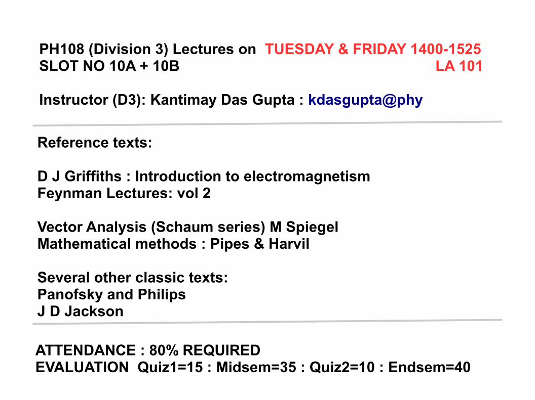
Reference texts:
D J Griffiths : Introduction to electromagnetismFeynman Lectures: vol 2
Vector Analysis (Schaum series) M SpiegelMathematical methods : Pipes & Harvil
Several other classic texts:Panofsky and PhilipsJ D Jackson
PH108 (Division 3) Lectures on TUESDAY & FRIDAY 1400-1525 SLOT NO 10A + 10B LA 101
Instructor (D3): Kantimay Das Gupta : kdasgupta@phy
ATTENDANCE : 80% REQUIREDEVALUATION Quiz1=15 : Midsem=35 : Quiz2=10 : Endsem=40
Basic principles known for about 150 years.
Mature subject with a well defined structure.
Regime of validity well undesrtood.
Great success: explaining propagation & generation of electromagnetic radiation,Forces of adhesion and cohesion.
First example of a classical field theory....particles and fields both carry energy and Momentum
Fails when we go to atomic scale
Gravity and electromagnetism are markedly different too, though both have '' inverse square force“ laws.
Electromagnetism
Two key questions:
Why do we use vectors?Why do we use many co-ordinate systems?
Symmetry of the problem and the shape of the objects involved must be taken into account.
What is a field ? What are the typical questions one asks?
A quantity defined or measured over a certain area/volume of space.
Scalar field Temperature defined over a region T(x,y,z)
Vector field Electric, Magnetic field : E(x,y,z) B(x,y,z) velocity of water v(x,y,z) in a pipe, river, ocean
Matrix/Tensor field Stress, Strain inside a material like a concrete beam. With every point a matrix like object is associated.
A field is also like an object with a large number of degrees of freedom.
How is the field created? What is the ''source'' ?How does the field affect particles in it (Interaction of field with matter)?
A systematic way of handling co-ordinate systems : Part 1
Many types of co-ordinates are needed, so that we can use the natural symmetry of a problem.
Equations would have the simplest form and minimum number of free variables if the co-ordinate system is chosen intelligently.
How to define a co-ordinate system?
Few typical systems:
Plane PolarSpherical PolarCylindrical
Then how to define your own if you need?
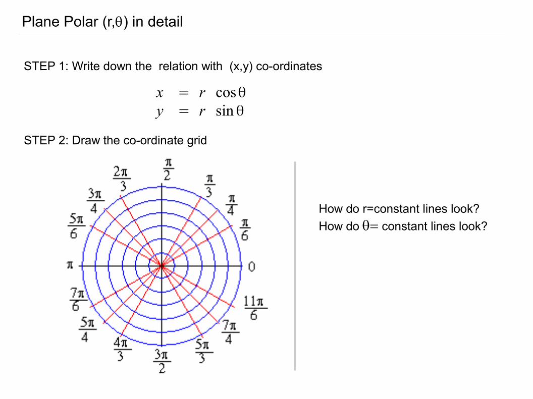
Plane Polar (r,q) in detail
STEP 1: Write down the relation with (x,y) co-ordinates
x = r cosθy = r sinθ
STEP 2: Draw the co-ordinate grid
How do r=constant lines look?
How do q= constant lines look?
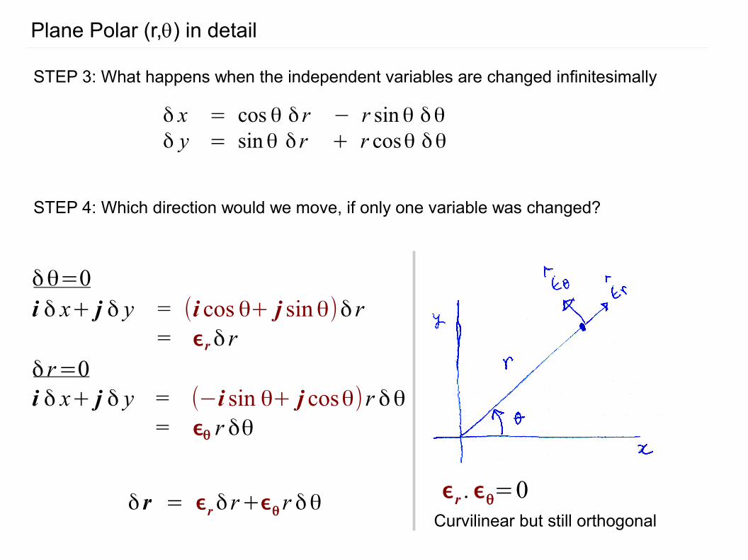
STEP 3: What happens when the independent variables are changed infinitesimally
Plane Polar (r,q) in detail
δ x = cos θ δ r − r sinθ δθδ y = sinθ δ r + r cosθ δθ
STEP 4: Which direction would we move, if only one variable was changed?
δθ=0i δ x+ j δ y = (i cos θ+ j sinθ)δ r
= ϵrδ rδ r=0i δ x+ j δ y = (−i sin θ+ j cosθ)r δθ
= ϵθ r δθ
ϵr .ϵθ=0Curvilinear but still orthogonal
δ r = ϵrδ r+ϵθ r δθ
Plane Polar (r,q) in detail
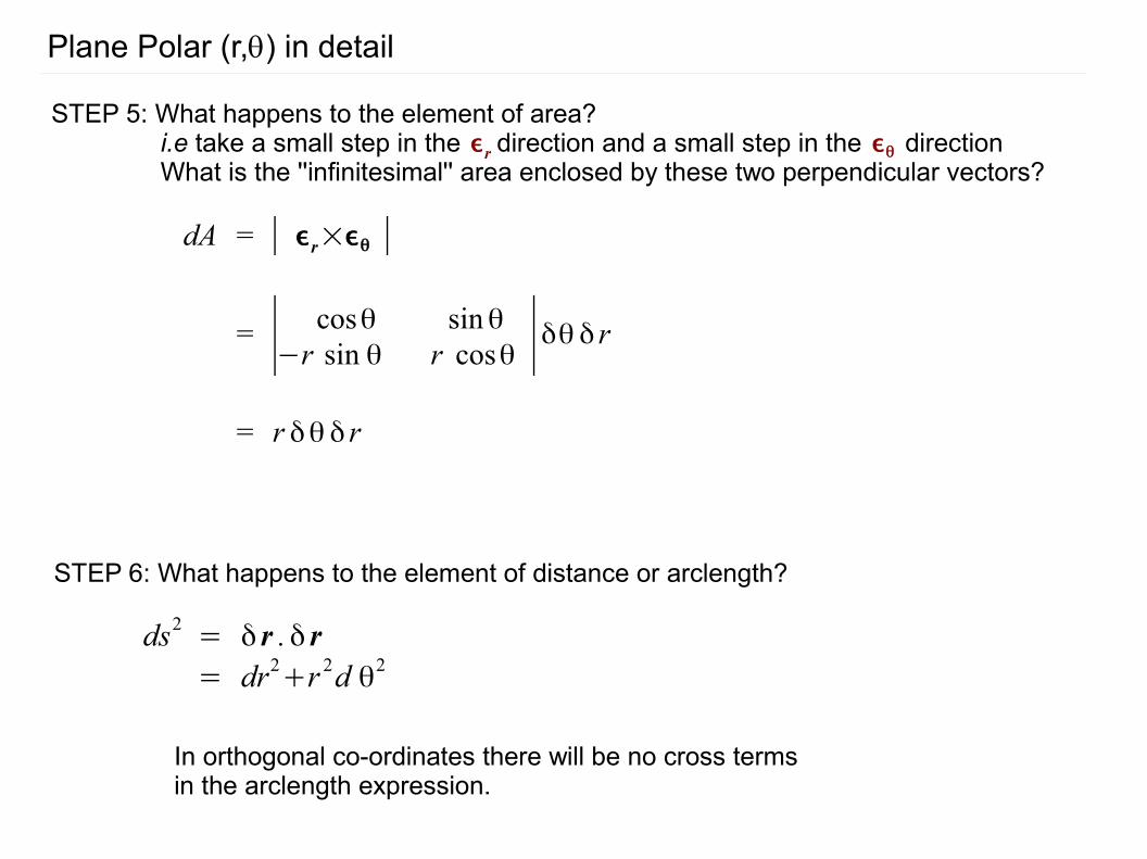
STEP 5: What happens to the element of area? i.e take a small step in the direction and a small step in the direction What is the ''infinitesimal'' area enclosed by these two perpendicular vectors?
ϵr ϵθ
dA = ∣ ϵr×ϵθ ∣
= ∣ cosθ sinθ−r sin θ r cosθ ∣δθ δ r
= r δθ δ r
STEP 6: What happens to the element of distance or arclength?
ds2= δ r .δ r= dr2
+r 2d θ2
In orthogonal co-ordinates there will be no cross terms in the arclength expression.
Plane Polar (r,q) in detail
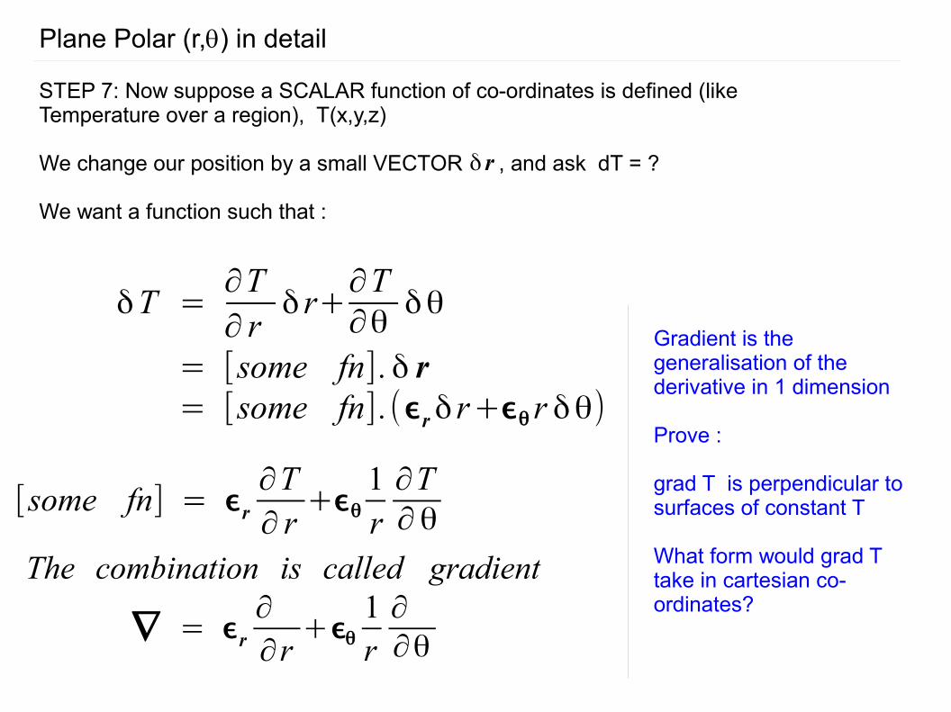
STEP 7: Now suppose a SCALAR function of co-ordinates is defined (like Temperature over a region), T(x,y,z)
We change our position by a small VECTOR , and ask dT = ?
We want a function such that :
δ r
δT =∂T∂ r
δ r+∂T∂θ
δθ
= [some fn] .δ r= [some fn] .(ϵrδ r+ϵθ r δθ)
[some fn] = ϵr∂T∂ r
+ϵθ1r∂T∂θ
The combination is called gradient
∇ = ϵr∂
∂r+ϵθ
1r∂∂θ
Gradient is the generalisation of the derivative in 1 dimension
Prove :
grad T is perpendicular to surfaces of constant T
What form would grad Ttake in cartesian co-ordinates?
Plane Polar (r,q) in detail
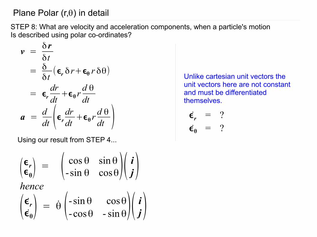
STEP 8: What are velocity and acceleration components, when a particle's motionIs described using polar co-ordinates?
v =δ rδt
= δδt(ϵr δ r+ϵθ r δθ)
= ϵrdrdt+ϵθ r
d θdt
a =ddt (ϵrdrdt +ϵθ r d θdt )
Unlike cartesian unit vectors the unit vectors here are not constant and must be differentiated themselves.
ϵr = ?ϵθ = ?
Using our result from STEP 4...
(ϵrϵθ) = ( cos θ sinθ-sin θ cosθ)( ij)
hence
(ϵrϵθ) = θ (-sinθ cosθ-cosθ - sinθ)( ij)

Plane Polar (r,q) in detail
STEP 8: What are velocity and acceleration components, when a particle's motionIs described using polar co-ordinates?
v =δ rδt
= δδt(ϵr δ r+ϵθ r δθ)
= ϵrdrdt+ϵθ r
d θdt
a =ddt (ϵrdrdt +ϵθ r d θdt )
Unlike cartesian unit vectors the unit vectors here are not constant and must be differentiated themselves.
ϵr = ?ϵθ = ?
Using our result from STEP 4...
(ϵrϵθ) = ( cos θ sinθ-sin θ cosθ)( ij)
hence
(ϵrϵθ) = θ (-sinθ cosθ-cosθ - sinθ)( ij)
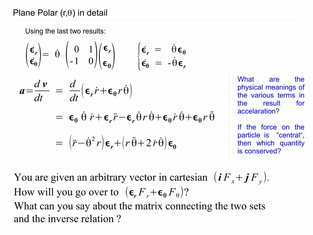
(ϵrϵθ)= θ ( 0 1-1 0)(
ϵr
ϵθ) {ϵr = θϵθϵθ = - θϵr
Using the last two results:
a=d vdt
=ddt(ϵr r+ϵθ r θ)
= ϵθ θ r+ϵr r−ϵr θr θ+ϵθ r θ+ϵθ r θ
= (r−θ2 r)ϵr+(r θ+2 r θ)ϵθ
Plane Polar (r,q) in detail
What are the physical meanings of the various terms in the result for accelaration?
If the force on the particle is “central“, then which quantity is conserved?
You are given an arbitrary vector in cartesian ( i F x+ j F y ).How will you go over to (ϵr F r+ϵθ Fθ)?What can you say about the matrix connecting the two setsand the inverse relation ?
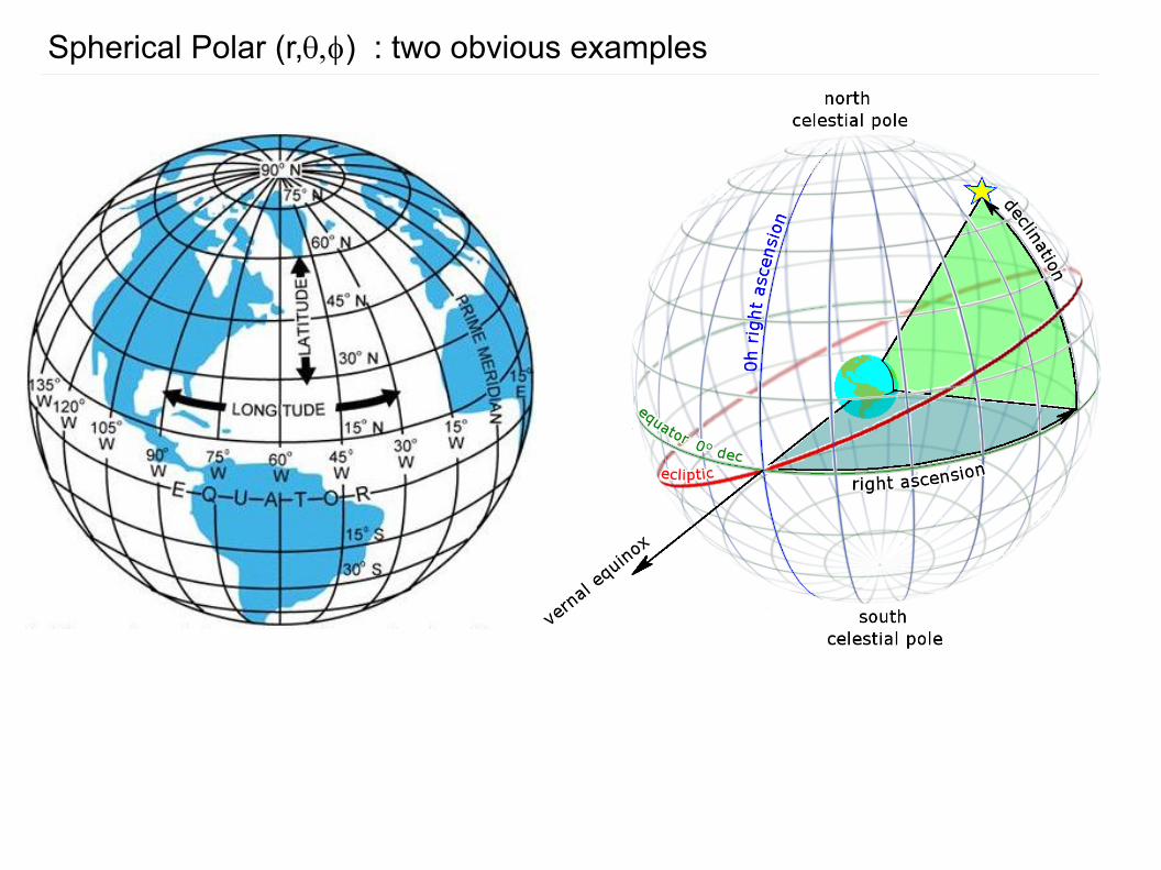
Spherical Polar (r,q,f) : two obvious examples
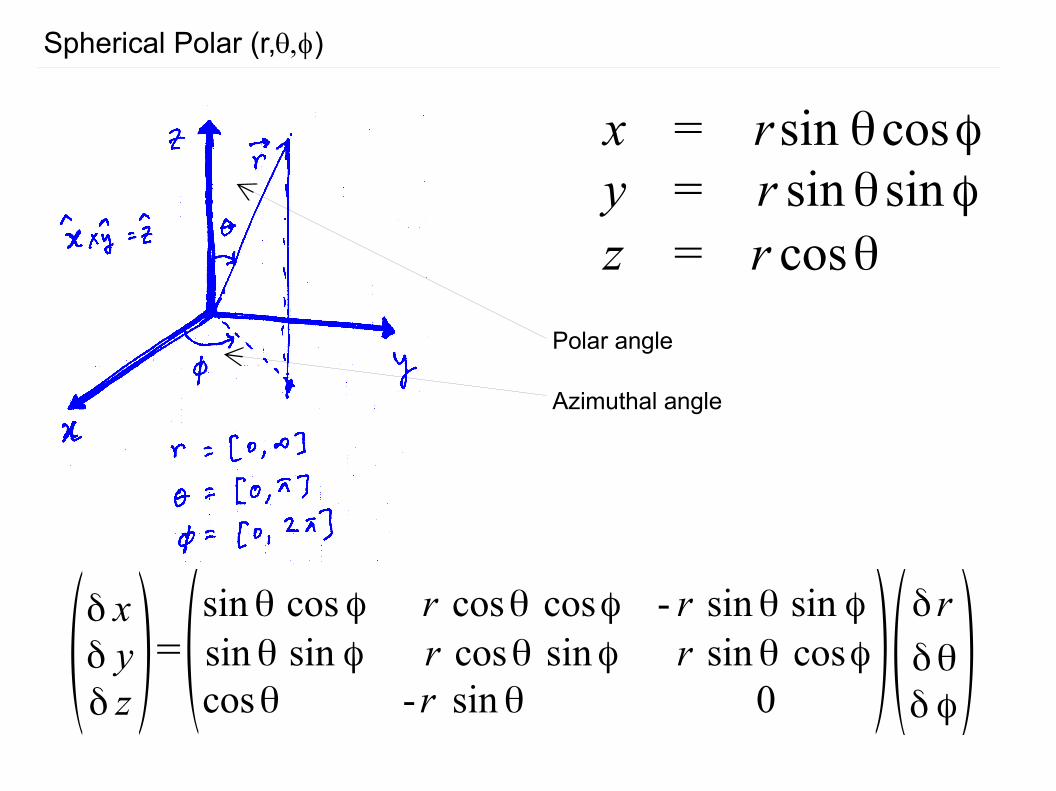
x = rsin θcosϕy = r sinθsinϕz = r cosθ
(δ xδ yδ z)=(
sinθ cos ϕ r cosθ cosϕ - r sinθ sin ϕsinθ sin ϕ r cosθ sinϕ r sinθ cosϕcosθ -r sinθ 0 )(
δ rδθδ ϕ)
Spherical Polar (r,q,f)
Polar angle
Azimuthal angle
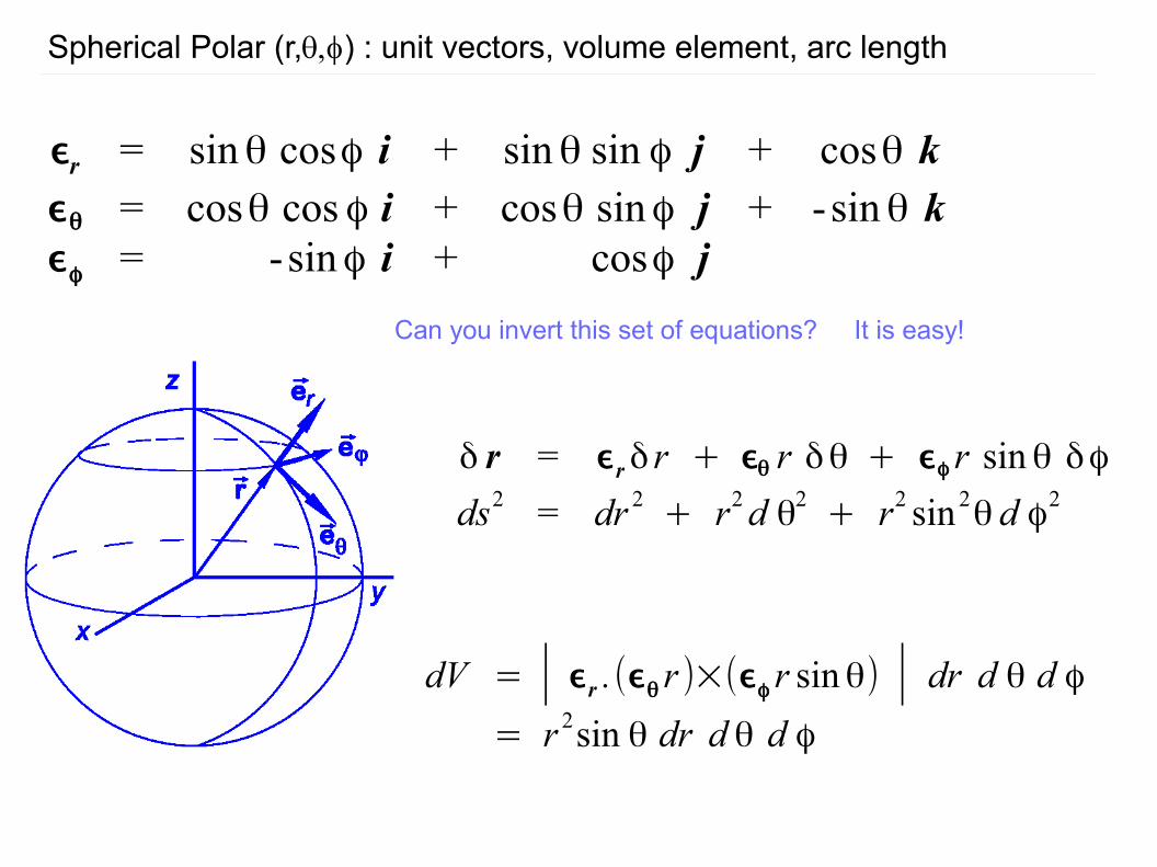
Spherical Polar (r,q,f) : unit vectors, volume element, arc length
ϵr = sinθ cosϕ i + sinθ sin ϕ j + cosθ kϵθ = cosθ cos ϕ i + cosθ sinϕ j + -sinθ kϵϕ = -sinϕ i + cosϕ j
δ r = ϵrδ r + ϵθ r δθ + ϵϕr sinθ δϕ
ds2 = dr 2+ r2d θ2
+ r2 sin 2θ d ϕ2
dV = ∣ ϵr .(ϵθ r )×(ϵϕ r sinθ) ∣ dr d θ d ϕ= r 2sin θ dr d θ d ϕ
Can you invert this set of equations? It is easy!
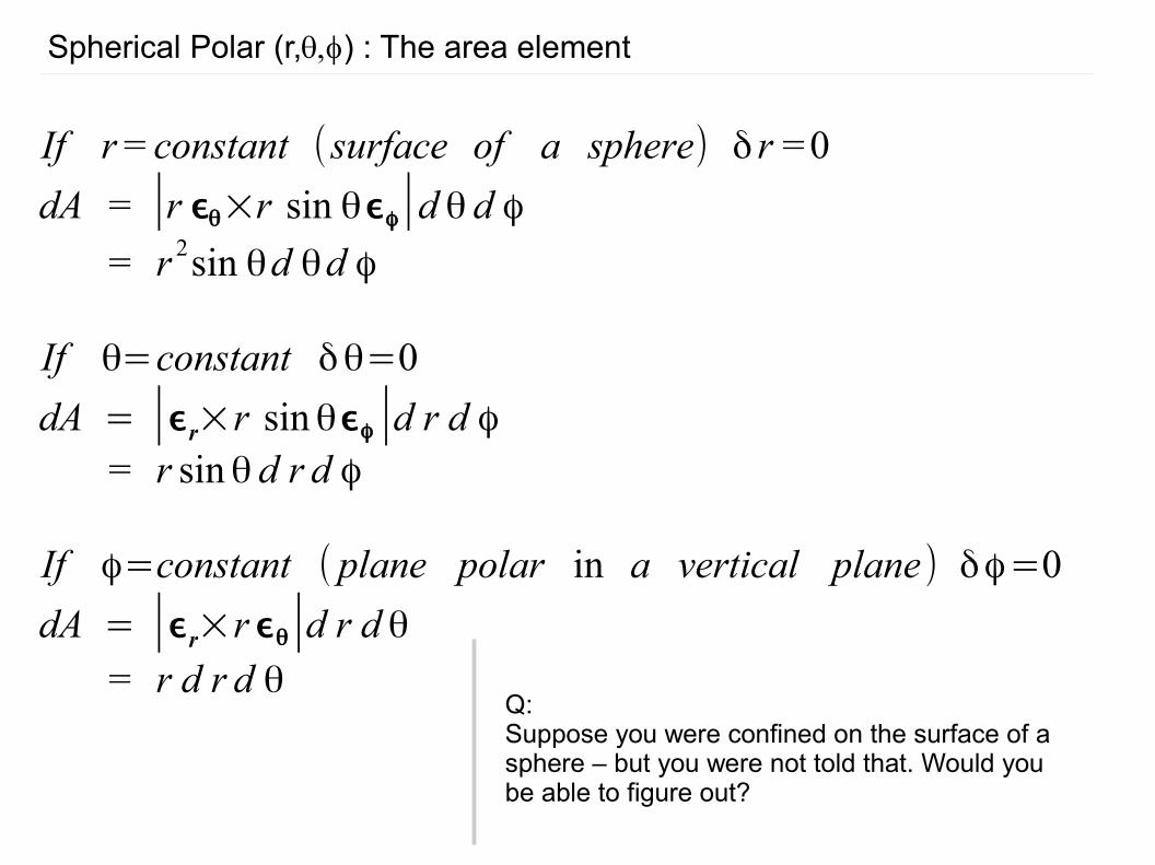
Spherical Polar (r,q,f) : The area element
If r = constant (surface of a sphere) δ r = 0
dA = ∣r ϵθ×r sin θϵϕ∣d θ d ϕ= r 2sin θd θd ϕ
If θ=constant δθ=0
dA = ∣ϵr×r sinθϵϕ∣d r d ϕ= r sinθ d r d ϕ
If ϕ=constant ( plane polar in a vertical plane) δϕ=0
dA = ∣ϵr×r ϵθ∣d r d θ= r d r d θ
Q:Suppose you were confined on the surface of a sphere – but you were not told that. Would you be able to figure out?
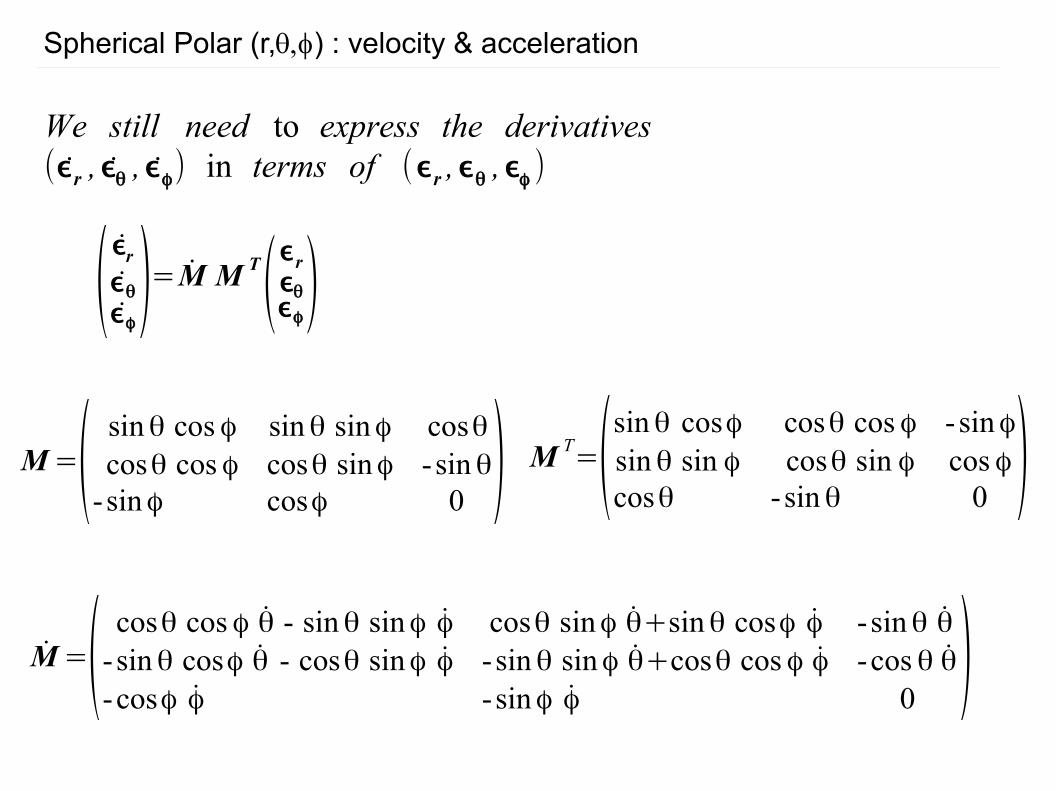
Spherical Polar (r,q,f) : velocity & acceleration
We still need to express the derivatives(ϵr , ϵθ , ϵϕ) in terms of (ϵr ,ϵθ ,ϵϕ )
M=(sinθ cos ϕ sinθ sinϕ cosθcosθ cos ϕ cosθ sinϕ -sinθ
-sinϕ cosϕ 0 )
M=(cosθ cos ϕ θ - sinθ sinϕ ϕ cosθ sinϕ θ+sinθ cosϕ ϕ -sinθ θ
-sinθ cosϕ θ - cosθ sinϕ ϕ -sinθ sinϕ θ+cosθ cos ϕ ϕ -cos θ θ-cosϕ ϕ -sinϕ ϕ 0 )
(ϵrϵθϵϕ)=M M T(
ϵrϵθϵϕ)
M T=(
sinθ cosϕ cosθ cos ϕ - sinϕsinθ sin ϕ cosθ sin ϕ cos ϕcosθ -sinθ 0 )
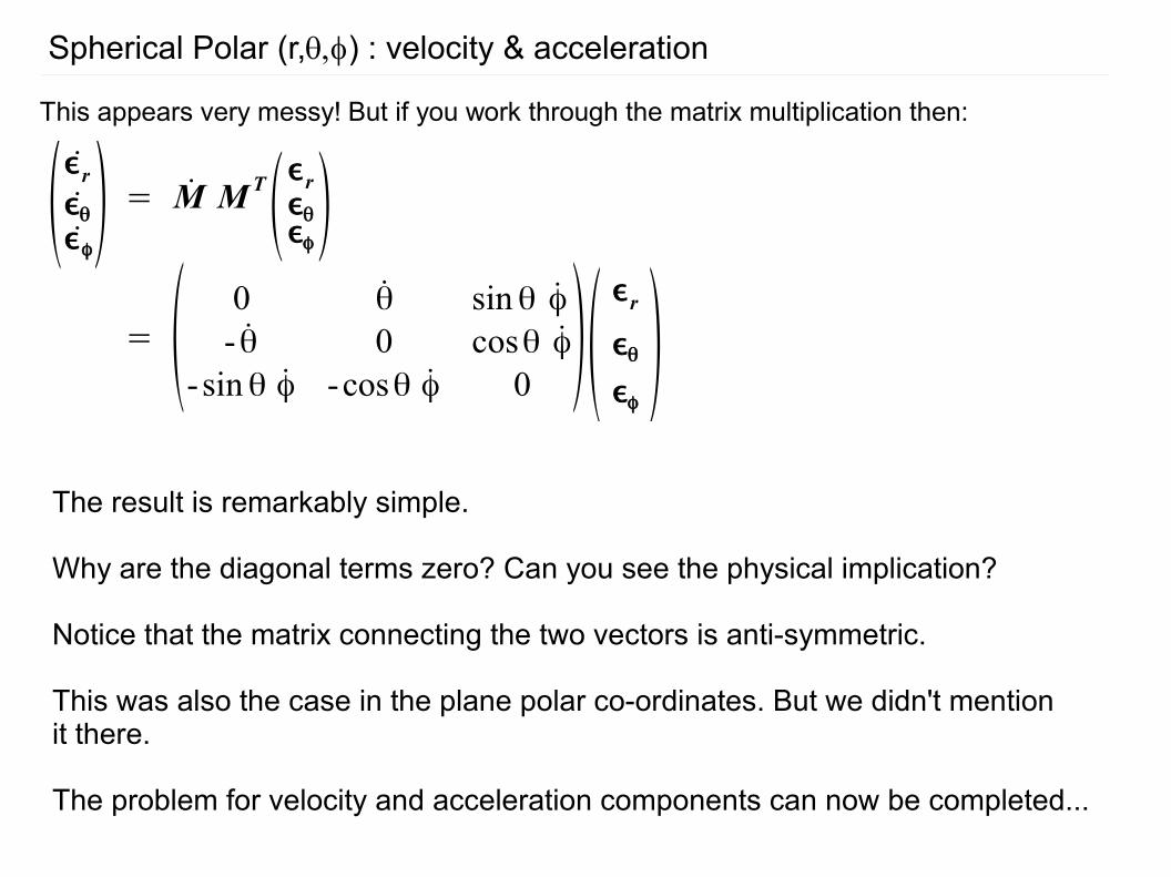
Spherical Polar (r,q,f) : velocity & acceleration
This appears very messy! But if you work through the matrix multiplication then:
(ϵrϵθϵϕ) = M MT(
ϵrϵθϵϕ)
= (0 θ sinθ ϕ
- θ 0 cosθ ϕ-sinθ ϕ -cosθ ϕ 0 )(
ϵr
ϵθϵϕ)
The result is remarkably simple.
Why are the diagonal terms zero? Can you see the physical implication?
Notice that the matrix connecting the two vectors is anti-symmetric.
This was also the case in the plane polar co-ordinates. But we didn't mentionit there.
The problem for velocity and acceleration components can now be completed...
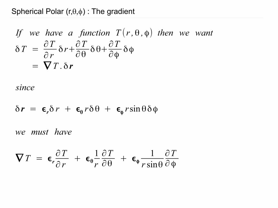
Spherical Polar (r,q,f) : The gradient
If we have a function T (r ,θ ,ϕ) then we want
δT =∂T∂ r
δ r+∂T∂θ
δθ+∂T∂ϕ
δϕ
= ∇ T .δ r
since
δ r = ϵrδ r + ϵθ rδθ + ϵϕ rsinθδϕ
we must have
∇ T = ϵr∂T∂ r
+ ϵθ1r∂T∂θ
+ ϵϕ1
r sinθ∂T∂ϕ
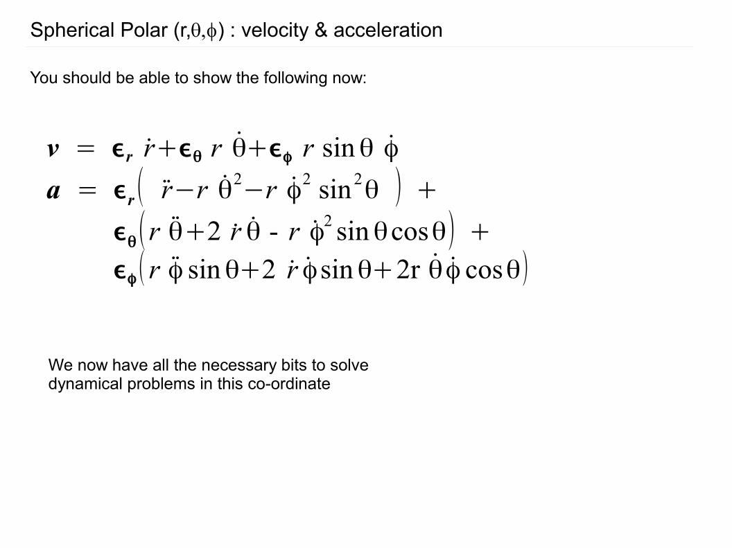
Spherical Polar (r,q,f) : velocity & acceleration
You should be able to show the following now:
v = ϵr r+ϵθ r θ+ϵϕ r sinθ ϕ
a = ϵr( r−r θ2−r ϕ2 sin2
θ ) +ϵθ(r θ+2 r θ - r ϕ2 sinθcosθ) +ϵϕ( r ϕ sinθ+2 r ϕsinθ+2r θ ϕ cosθ)
We now have all the necessary bits to solve dynamical problems in this co-ordinate
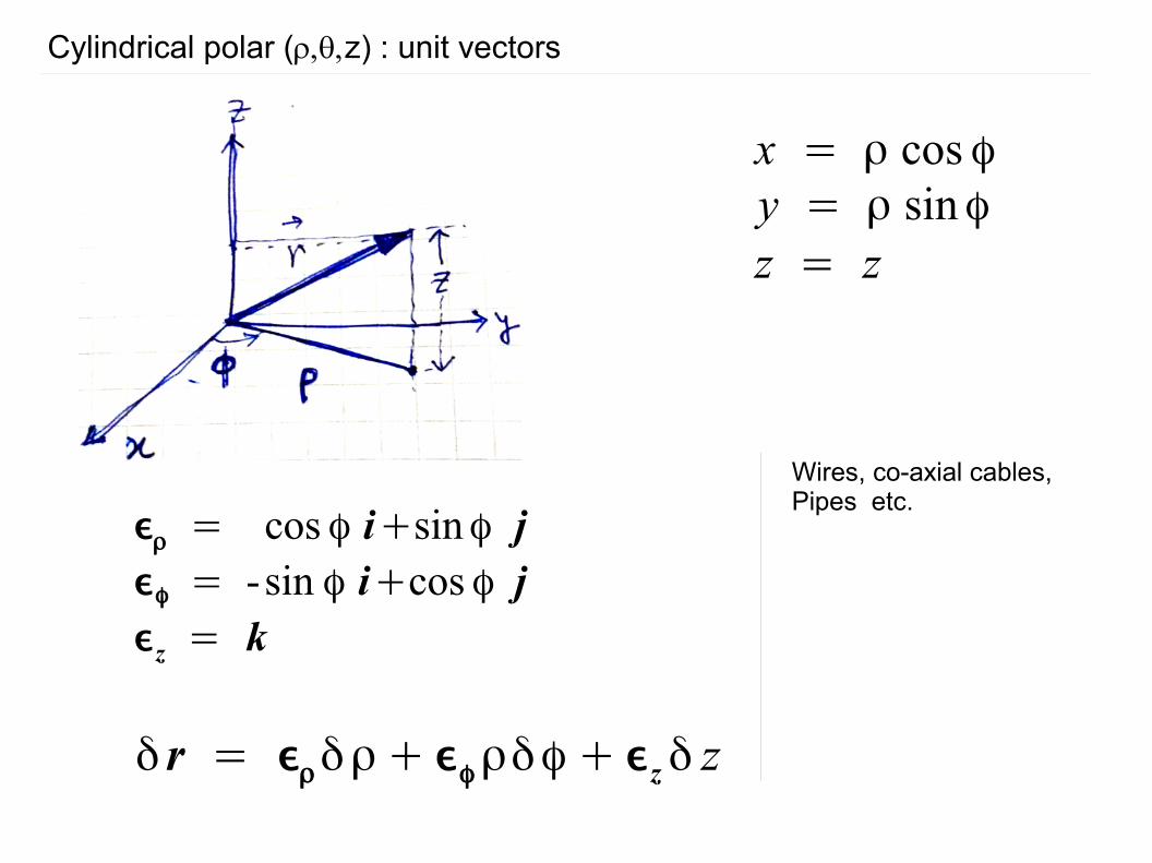
Cylindrical polar (r,q,z) : unit vectors
x = ρ cos ϕy = ρ sinϕz = z
Wires, co-axial cables,Pipes etc.
ϵρ = cos ϕ i+sinϕ jϵϕ = -sin ϕ i+cos ϕ jϵz = k
δ r = ϵρδρ + ϵϕρδϕ + ϵzδ z
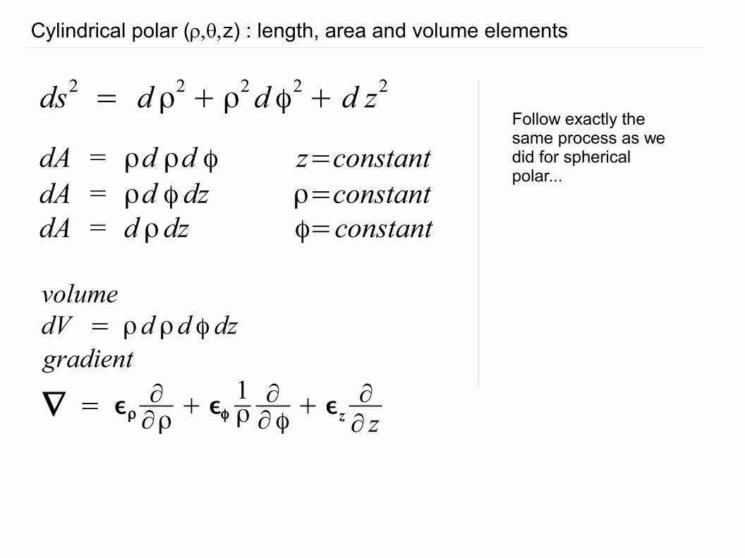
Cylindrical polar (r,q,z) : length, area and volume elements
ds2= d ρ2
+ ρ2d ϕ2
+ d z2
dA = ρd ρd ϕ z=constantdA = ρd ϕdz ρ=constantdA = d ρdz ϕ=constant
volumedV = ρd ρd ϕdzgradient
∇ = ϵρ∂∂ρ
+ ϵϕ1ρ∂∂ϕ
+ ϵz∂∂ z
Follow exactly the same process as we did for spherical polar...
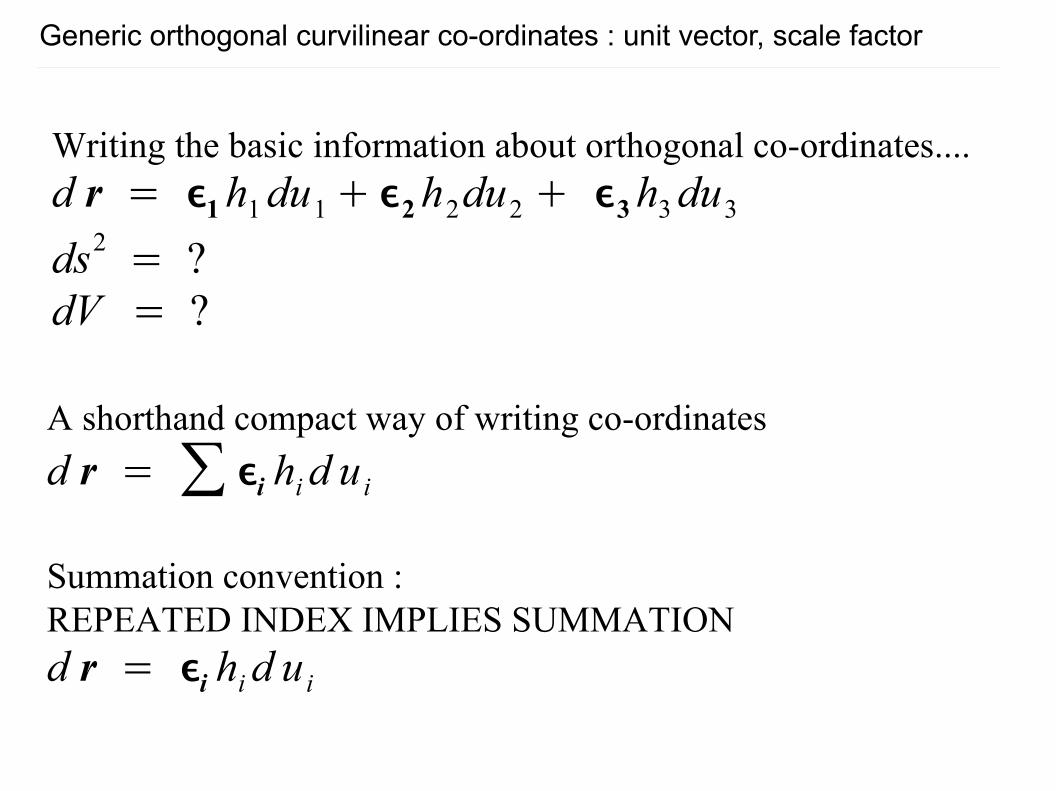
Writing the basic information about orthogonal co-ordinates....d r = ϵ1h1du1+ ϵ2h2du2 + ϵ3h3du3
ds2= ?
dV = ?
Generic orthogonal curvilinear co-ordinates : unit vector, scale factor
A shorthand compact way of writing co-ordinates
d r = ∑ ϵi hid u i
Summation convention :REPEATED INDEX IMPLIES SUMMATIONd r = ϵi hid u i
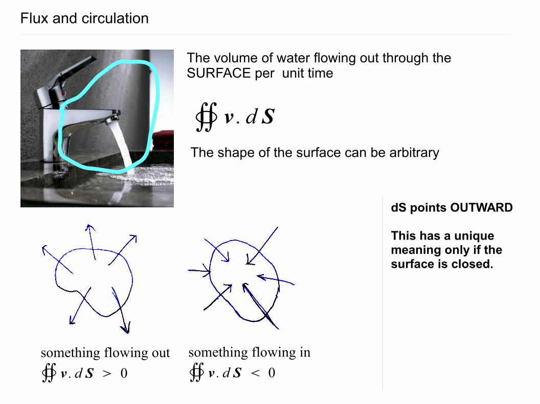
Flux and circulation
The volume of water flowing out through the SURFACE per unit time
∯ v . d S
The shape of the surface can be arbitrary
something flowing out
∯ v . d S > 0
something flowing in
∯ v . d S < 0
dS points OUTWARD
This has a unique meaning only if the surface is closed.
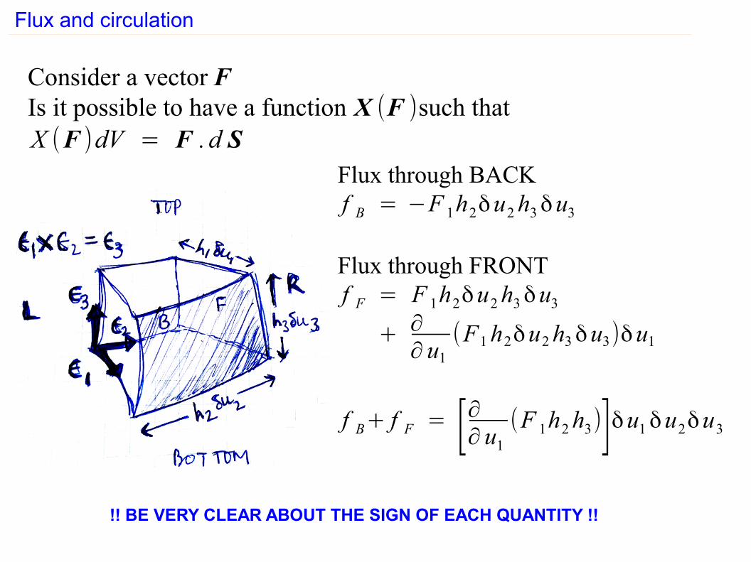
Flux and circulation
Consider a vector FIs it possible to have a function X (F )such thatX (F )dV = F . d S
Flux through BACKf B = −F 1h2δu2h3δu3
Flux through FRONTf F = F 1h2δu2h3δu3
+ ∂∂ u1
(F1h2δu2h3δu3)δu1
f B+ f F = [∂∂ u1
(F 1h2h3)]δu1δu2δu3
!! BE VERY CLEAR ABOUT THE SIGN OF EACH QUANTITY !!
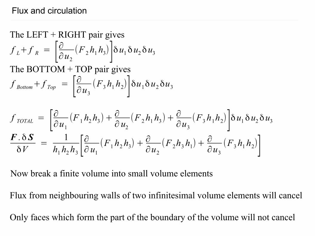
Flux and circulation
The LEFT + RIGHT pair gives
f L+ f R = [∂∂u2
(F 2h1h3)]δu1δu2δu3
The BOTTOM + TOP pair gives
f Bottom+ f Top = [∂∂u3
(F3h1h2)]δu1δu2δu3
f TOTAL = [∂∂u1
(F 1h2h3)+∂∂ u2
(F 2h1h3)+∂∂u3
(F3h1h2)]δu1δu2δu3
F .δ SδV
=1
h1h2h3 [∂∂ u1
(F1h2h3) +∂∂u2
(F 2h3h1)+∂∂u3
(F3h1h2)]Now break a finite volume into small volume elements
Flux from neighbouring walls of two infinitesimal volume elements will cancel
Only faces which form the part of the boundary of the volume will not cancel
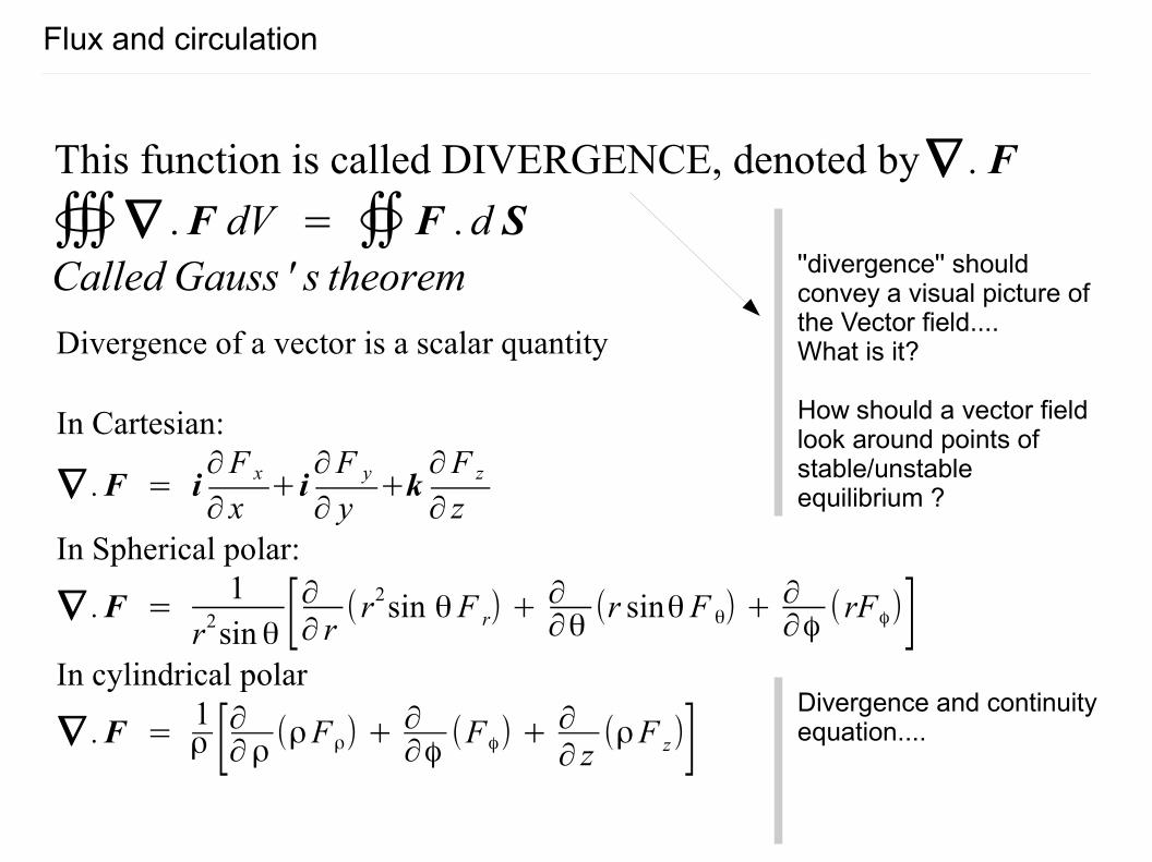
Divergence of a vector is a scalar quantity
In Cartesian:
∇ .F = i∂F x
∂ x+ i∂F y
∂ y+k
∂F z
∂ zIn Spherical polar:
∇ .F =1
r2sin θ [∂∂ r(r2sin θF r) +
∂∂θ
(r sinθF θ) +∂∂ϕ
(rFϕ)]In cylindrical polar
∇ .F =1ρ [∂∂ρ (ρFρ) +
∂∂ϕ
(Fϕ) +∂∂ z
(ρF z)]
Flux and circulation
This function is called DIVERGENCE, denoted by∇ .F
∰∇ .F dV = ∯F . d SCalled Gauss ' s theorem ''divergence'' should
convey a visual picture of the Vector field.... What is it?
How should a vector field look around points of stable/unstable equilibrium ?
Divergence and continuity equation....
Flux and circulation
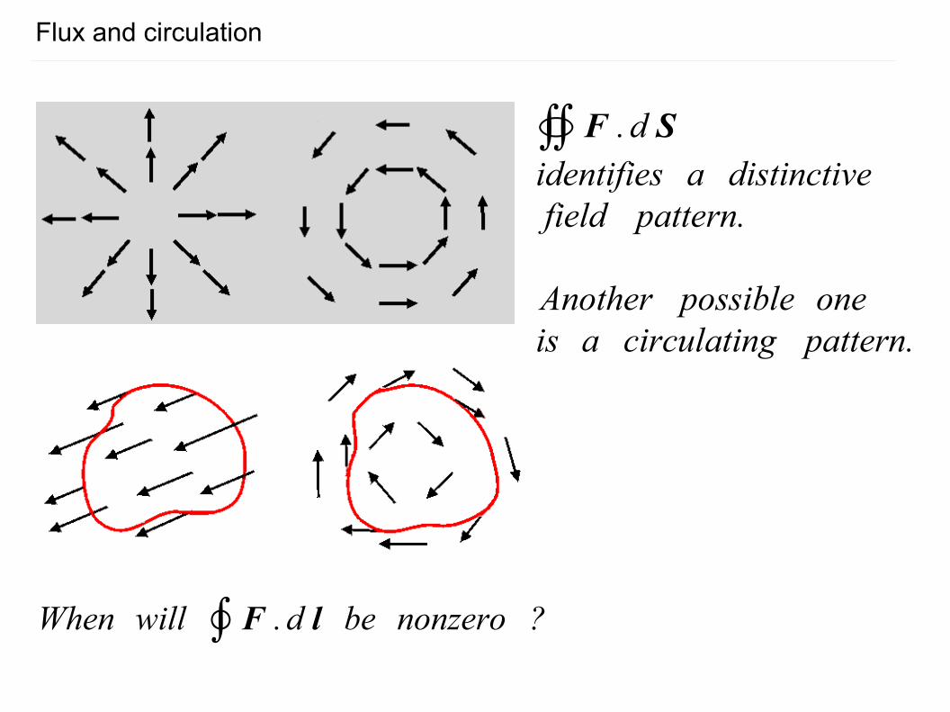
When will ∮F . d l be nonzero ?
∯F . d Sidentifies a distinctivefield pattern.
Another possible oneis a circulating pattern.
Flux and circulation
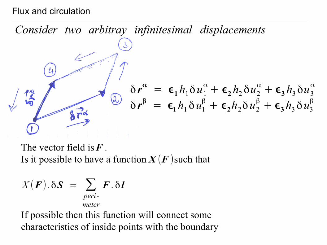
Consider two arbitray infinitesimal displacements
The vector field isF .Is it possible to have a function X (F )such that
X (F ) .δS = ∑peri -
meter
F .δ l
If possible then this function will connect somecharacteristics of inside points with the boundary
δ rα = ϵ1h1δu1α+ ϵ2h2δu2
α+ ϵ3h3δu3
α
δ rβ = ϵ1h1δu1β+ ϵ2h2δu2
β+ ϵ3h3δu3
β
Flux and circulation
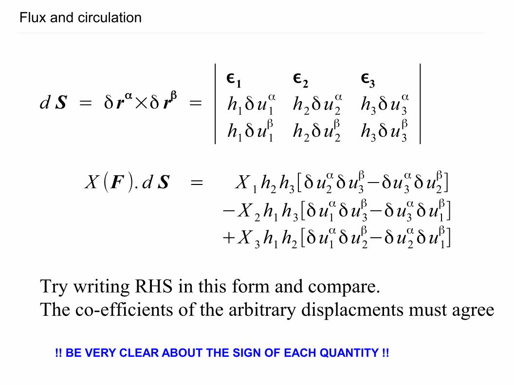
d S = δ rα×δ rβ = ∣ϵ1 ϵ2 ϵ3h1δu1
α h2δu2α h3δu3
α
h1δu1β h2δu2
β h3δu3β ∣
X (F ). d S = X 1h2h3[δu2αδu3
β−δu3
αδu2
β]
−X 2h1h3[δu1αδu3
β−δu3
αδu1
β]
+X 3h1h2 [δu1αδu2
β−δu2
αδu1
β]
Try writing RHS in this form and compare.The co-efficients of the arbitrary displacments must agree
!! BE VERY CLEAR ABOUT THE SIGN OF EACH QUANTITY !!
Flux and circulation
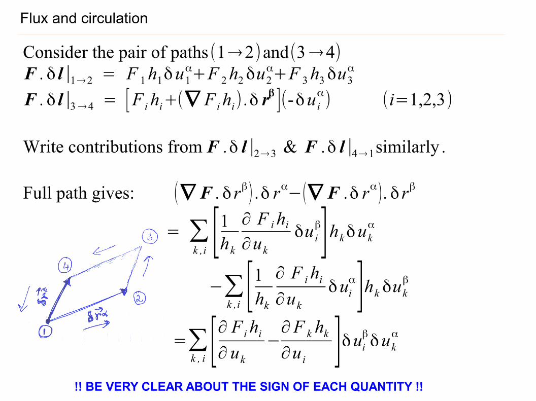
Consider the pair of paths(1→2)and(3→4)F .δ l∣1→2 = F 1h1δu1
α+F 2h2δu2α+F 3h3δu3
α
F .δ l∣3→4 = [F ihi+(∇ F ihi) .δ rβ ](-δu i
α) (i=1,2,3)
Write contributions from F .δ l∣2→3 & F .δ l∣4→1similarly .
Full path gives: (∇ F .δ rβ) .δ rα−(∇ F .δ rα).δ rβ
= ∑k ,i [
1hk
∂ F ihi∂uk
δu iβ]hkδukα
−∑k ,i [
1hk
∂ F ihi∂uk
δuiα]hk δukβ
=∑k , i [
∂ F ihi∂ uk
−∂F k hk∂u i ]δuiβδukα
!! BE VERY CLEAR ABOUT THE SIGN OF EACH QUANTITY !!
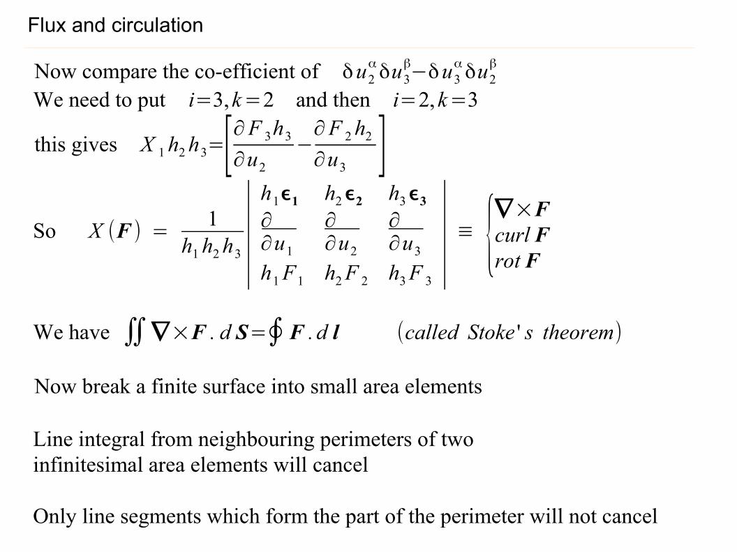
Flux and circulation
Now compare the co-efficient of δu2αδu3
β−δu3
αδu2
β
We need to put i=3,k=2 and then i=2,k=3
this gives X 1h2h3=[∂F 3h3
∂u2
−∂F 2h2
∂u3 ]So X (F ) =
1h1h2h3 ∣
h1ϵ1 h2 ϵ2 h3ϵ3∂∂u1
∂∂u2
∂∂u3
h1F1 h2F 2 h3F 3
∣ ≡ {∇×Fcurl Frot F
We have ∬∇×F . d S=∮F . d l (called Stoke ' s theorem)
Now break a finite surface into small area elements
Line integral from neighbouring perimeters of twoinfinitesimal area elements will cancel
Only line segments which form the part of the perimeter will not cancel
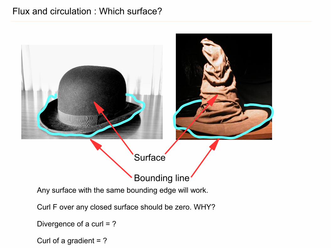
Flux and circulation : Which surface?
Surface
Bounding lineAny surface with the same bounding edge will work.
Curl F over any closed surface should be zero. WHY?
Divergence of a curl = ?
Curl of a gradient = ?
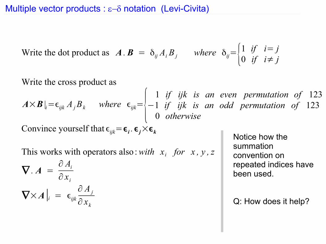
Multiple vector products : e-d notation (Levi-Civita)
Write the dot product as A .B = δij Ai B j where δij={1 if i= j0 if i≠ j
Write the cross product as
A×B |i=ϵijk A jB k where ϵijk={1 if ijk is an even permutation of 123
−1 if ijk is an odd permutation of 1230 otherwise
Convince yourself that ϵijk=ϵi .ϵ j×ϵk
This works with operators also :with x i for x , y , z
∇ . A =∂ Ai∂ x i
∇×A |i = ϵijk∂ A j
∂ xk
Notice how the summation convention on repeated indices have been used.
Q: How does it help?
Multiple vector products : e-d notation (Levi-Civita)
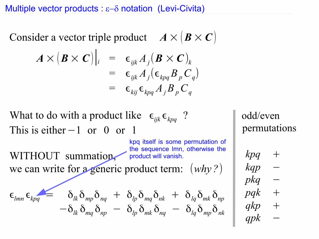
Consider a vector triple product A× (B× C )
A× (B× C )|i = ϵijk A j(B × C )k= ϵijk A j(ϵkpqB pCq)
= ϵkij ϵkpq A jB pCq
What to do with a product like ϵijk ϵkpq ?This is either−1 or 0 or 1
WITHOUT summation,we can write for a generic product term: (why?)
ϵlmn ϵkpq = δlkδmpδnq + δlpδmqδnk + δ lqδmk δnp−δlk δmqδnp − δlp δmk δnq − δlqδmpδnk
odd/evenpermutations
kpq +
kqp −pkq −
pqk +
qkp +qpk −
kpq itself is some permutation of the sequence lmn, otherwise the product will vanish.
Multiple vector products : e-d notation (Levi-Civita)
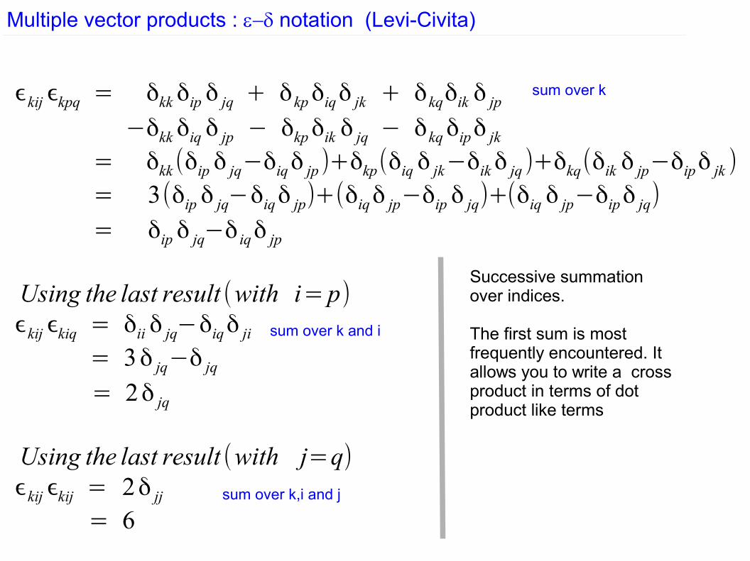
ϵkij ϵkpq = δkk δip δ jq + δkpδiqδ jk + δkqδik δ jp−δkk δiq δ jp − δkpδik δ jq − δkqδipδ jk
= δkk(δip δ jq−δiqδ jp)+δkp(δiq δ jk−δikδ jq )+δkq(δik δ jp−δipδ jk )
= 3(δip δ jq−δiqδ jp)+(δiqδ jp−δip δ jq)+(δiq δ jp−δipδ jq)= δip δ jq−δ iqδ jp
Using the last result (with i=p)ϵkij ϵkiq = δii δ jq−δiqδ ji
= 3δ jq−δ jq= 2δ jq
Using the last result (with j=q)ϵkij ϵkij = 2δ jj
= 6
Successive summation over indices.
The first sum is most frequently encountered. It allows you to write a cross product in terms of dot product like terms
sum over k
sum over k and i
sum over k,i and j
Multiple vector products : e-d notation (Levi-Civita)
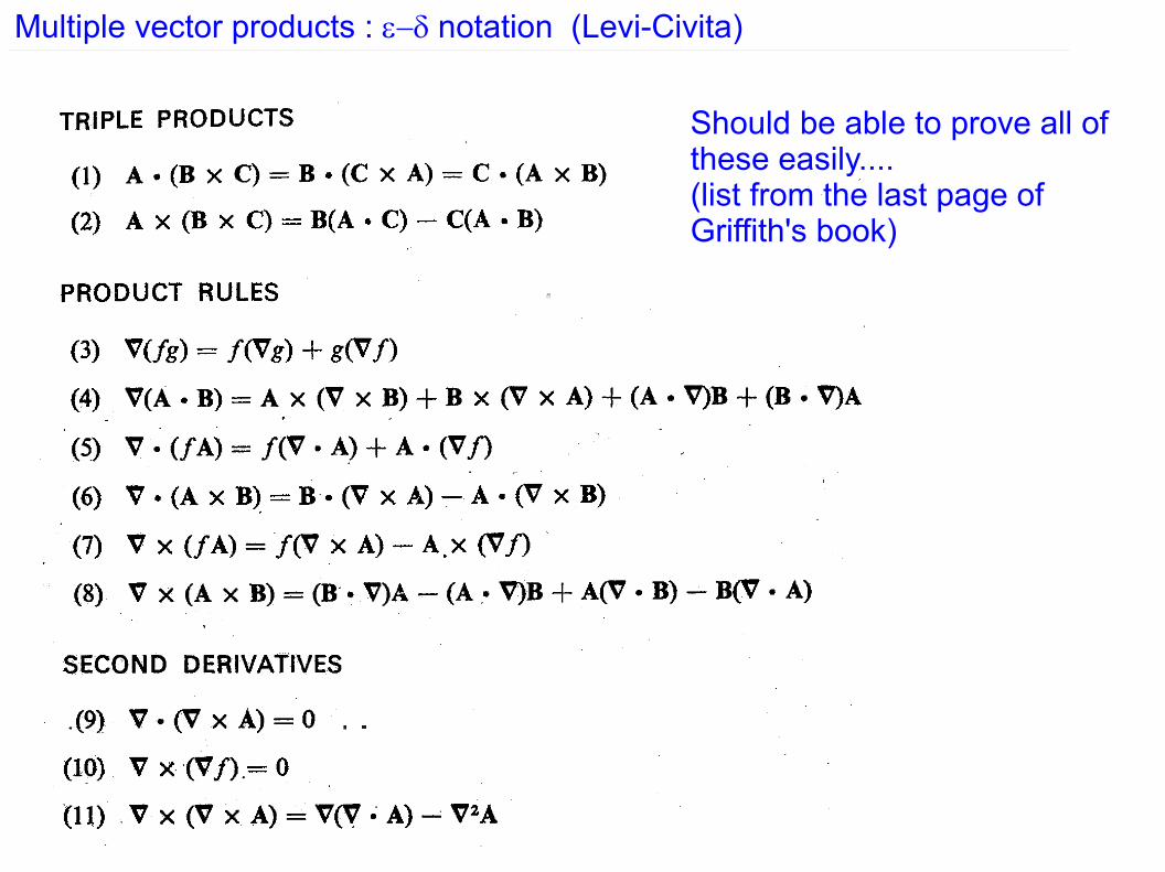
Should be able to prove all of these easily....(list from the last page of Griffith's book)
Co-ordinate systems, transformations etc : few problems
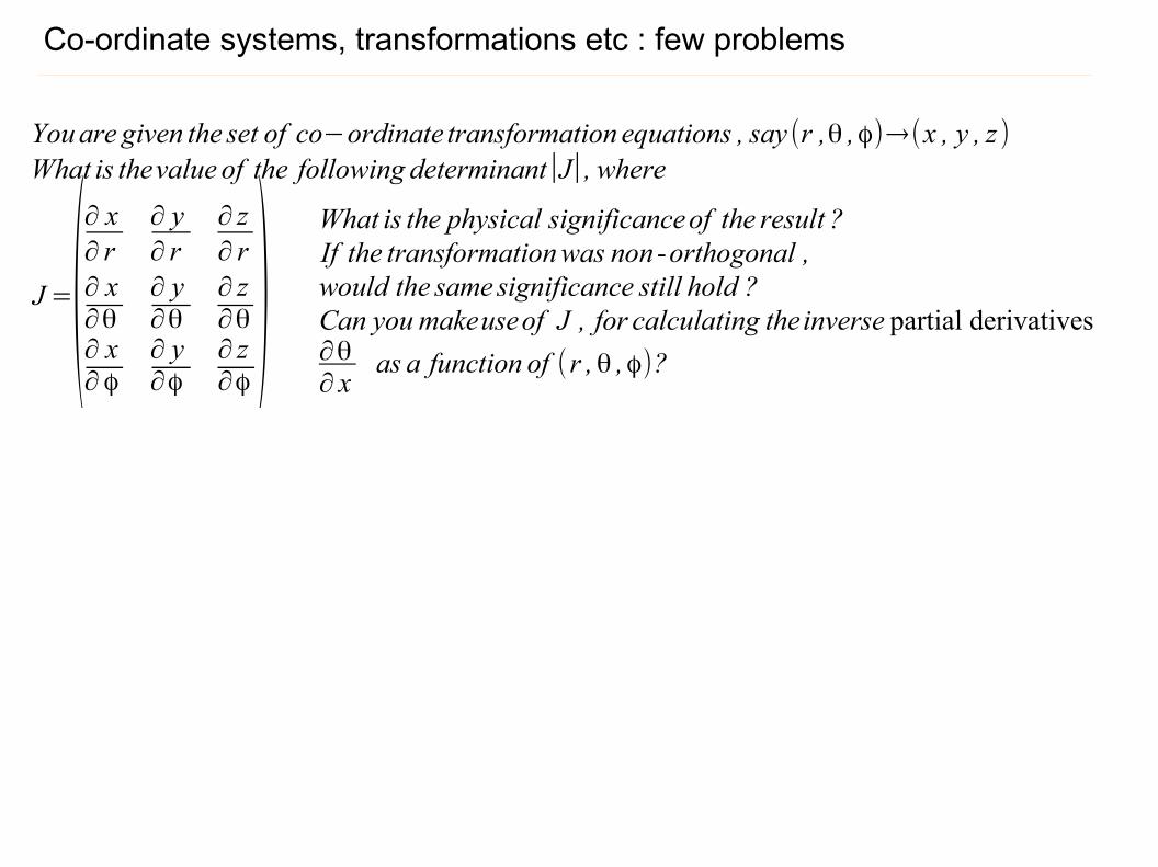
Youare given the set of co−ordinate transformation equations , say (r ,θ ,ϕ)→(x , y , z )What is thevalue of the following determinant∣J∣, where
J=(∂ x∂ r
∂ y∂ r
∂ z∂ r
∂ x∂θ
∂ y∂θ
∂ z∂θ
∂ x∂ϕ
∂ y∂ϕ
∂ z∂ϕ)
What is the physical significanceof the result ?If the transformationwas non -orthogonal ,would the same significance still hold ?Can you makeuseof J , for calculating theinverse partial derivatives∂θ∂ x
as a function of (r ,θ ,ϕ)?
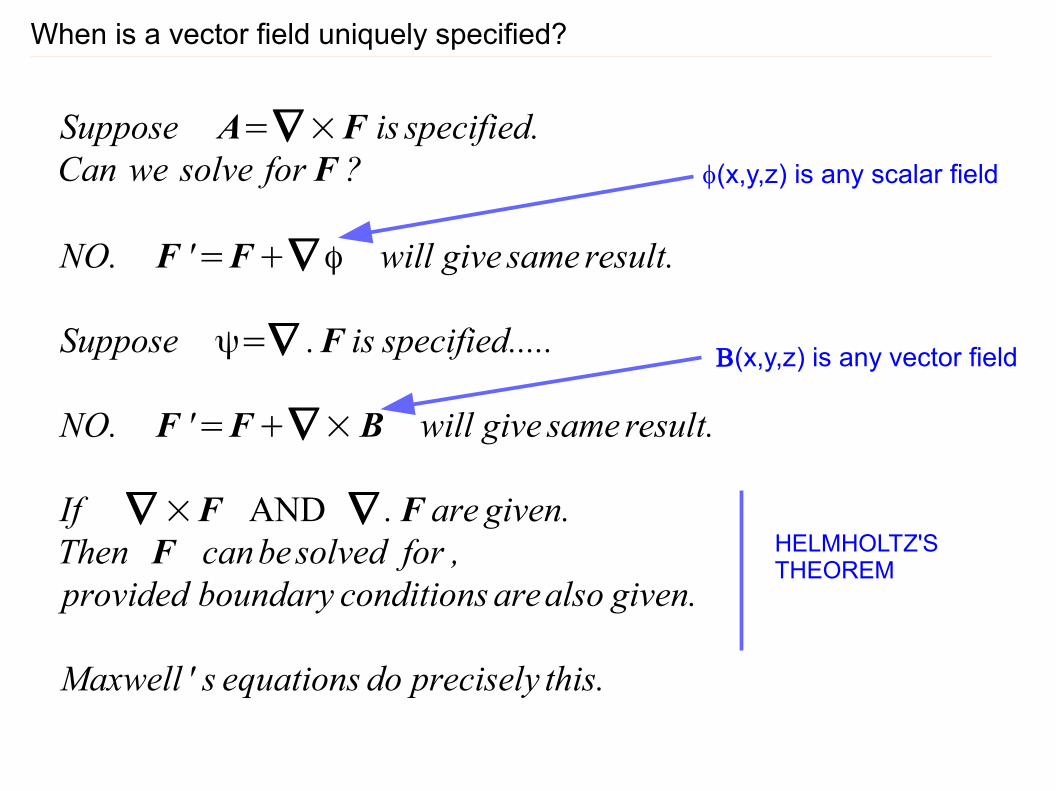
When is a vector field uniquely specified?
Suppose A=∇×F is specified.Can we solve for F ?
NO. F '=F+∇ϕ will give same result.
Suppose ψ=∇ .F is specified.....
NO. F '=F+∇× B will give same result.
If ∇ ×F AND ∇ .F are given.Then F canbesolved for ,provided boundary conditions arealso given.
Maxwell ' s equations do precisely this.
f(x,y,z) is any scalar field
B(x,y,z) is any vector field
HELMHOLTZ'STHEOREM

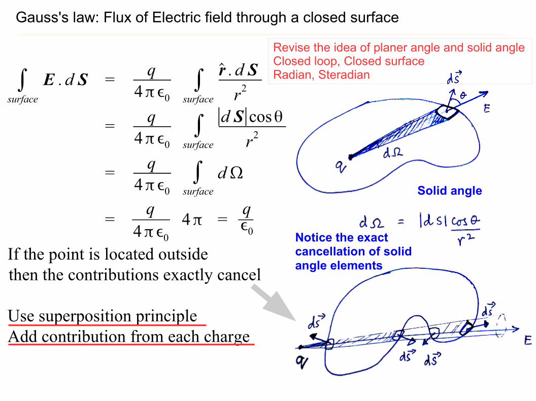
Gauss's law: Flux of Electric field through a closed surface
∫surface
E . d S =q
4πϵ0∫
surface
r . d S
r2
=q
4πϵ0∫
surface
∣d S∣cosθ
r2
=q
4πϵ0∫
surface
dΩ
=q
4πϵ0
4π =qϵ0
If the point is located outsidethen the contributions exactly cancel
Use superposition principleAdd contribution from each charge
Solid angle
Notice the exact cancellation of solid angle elements
Revise the idea of planer angle and solid angleClosed loop, Closed surfaceRadian, Steradian
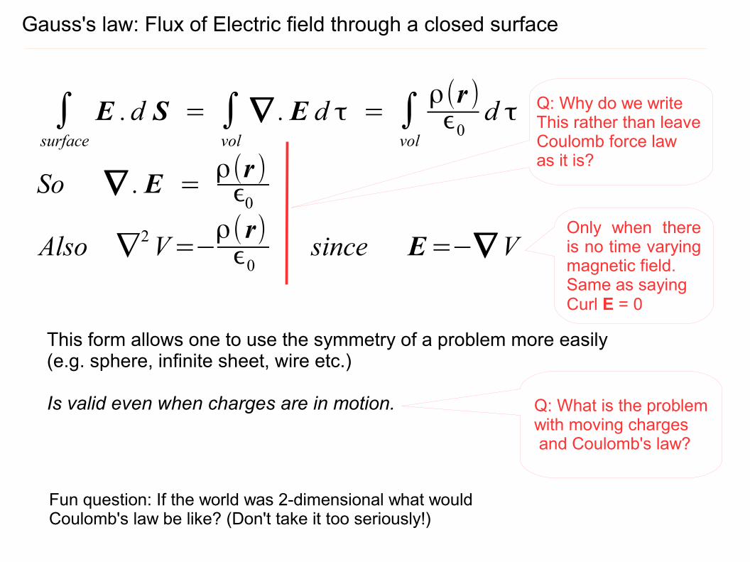
Gauss's law: Flux of Electric field through a closed surface
∫surface
E . d S = ∫vol
∇ .E d τ = ∫vol
ρ(r )ϵ0
d τ
So ∇ .E =ρ(r )ϵ0
Also ∇2V=−
ρ(r)ϵ0
since E=−∇VOnly when there is no time varying magnetic field.Same as sayingCurl E = 0
Q: Why do we write This rather than leave Coulomb force law as it is?
This form allows one to use the symmetry of a problem more easily(e.g. sphere, infinite sheet, wire etc.)
Is valid even when charges are in motion. Q: What is the problemwith moving charges and Coulomb's law?
Fun question: If the world was 2-dimensional what would Coulomb's law be like? (Don't take it too seriously!)
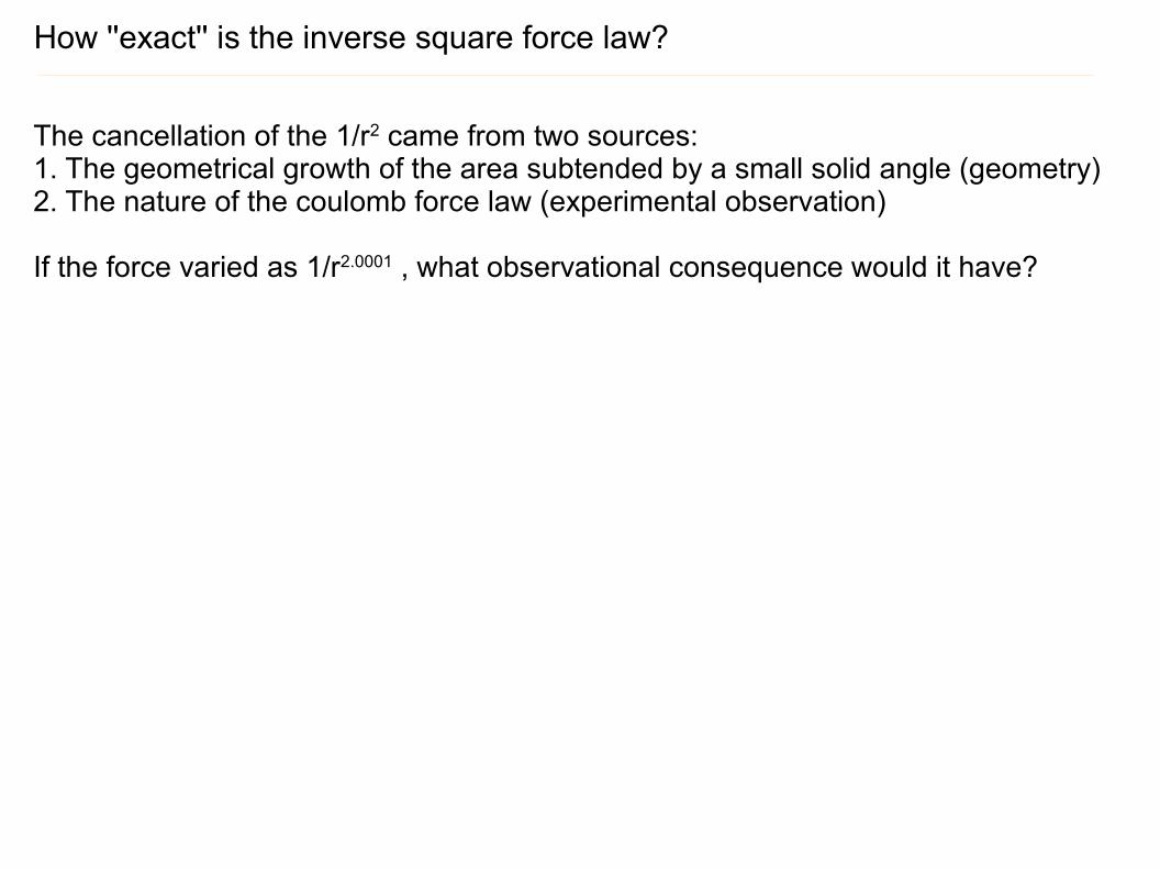
How ''exact'' is the inverse square force law?
The cancellation of the 1/r2 came from two sources:1. The geometrical growth of the area subtended by a small solid angle (geometry)2. The nature of the coulomb force law (experimental observation)
If the force varied as 1/r2.0001 , what observational consequence would it have?
Gauss's law: divergence of 1/r2 and the Dirac delta function
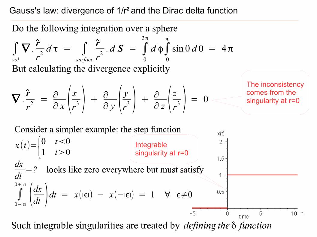
Do the following integration over a sphere
∫vol
∇ .r
r2d τ = ∫
surface
r
r2. d S = ∫
0
2π
d ϕ∫0
π
sinθ d θ = 4π
But calculating the divergence explicitly
∇ .r
r2 = ∂∂ x (xr3 ) + ∂
∂ y ( yr3 ) + ∂∂ z (zr3 ) = 0
The inconsistencycomes from the singularity at r=0
Consider a simpler example: the step function
x (t)={0 t<01 t>0
dxdt=? looks like zero everywhere but must satisfy
∫0−∣ϵ∣
0+∣ϵ∣
(dxdt )dt = x(∣ϵ∣) − x(−∣ϵ∣) = 1 ∀ ϵ≠0
Integrable singularity at r=0
Such integrable singularities are treated by defining the δ function
Gauss's law: divergence of 1/r2 and the Dirac delta function
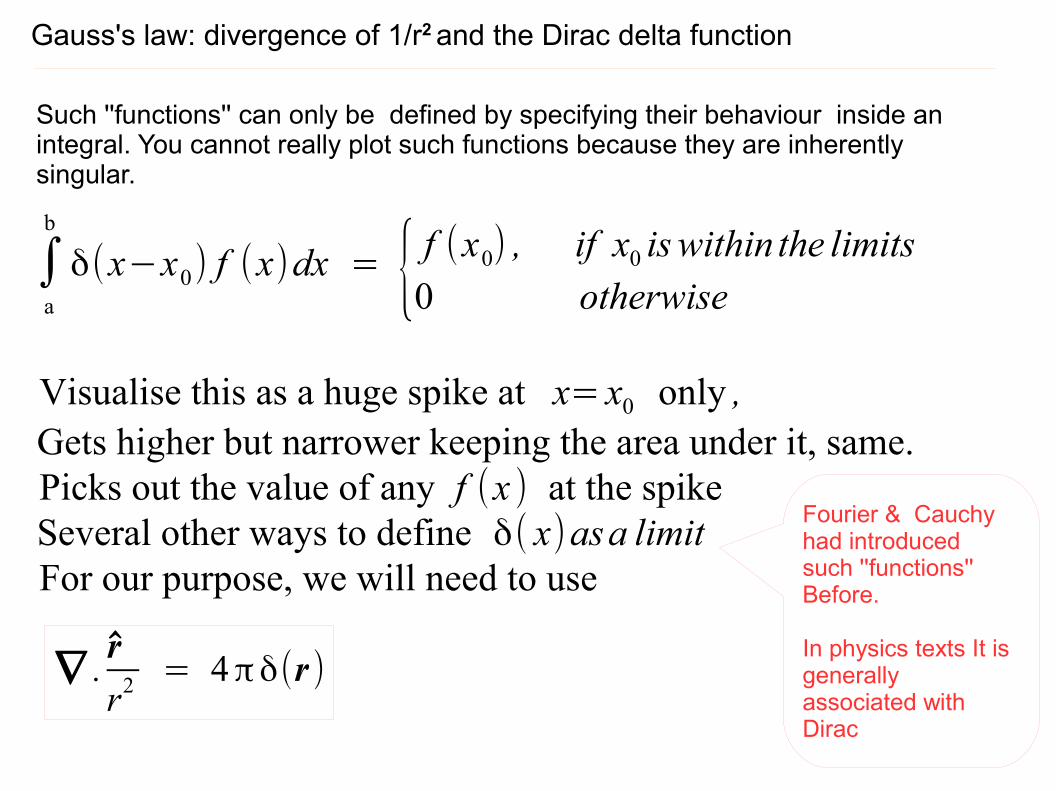
Such ''functions'' can only be defined by specifying their behaviour inside an integral. You cannot really plot such functions because they are inherently singular.
∫a
b
δ(x−x0) f (x)dx = { f (x0) , if x0 iswithin the limits0 otherwise
Visualise this as a huge spike at x= x0 only ,Gets higher but narrower keeping the area under it, same.Picks out the value of any f (x ) at the spikeSeveral other ways to define δ( x)asa limitFor our purpose, we will need to use
∇ .r
r2 = 4πδ(r )
Fourier & Cauchy had introduced such ''functions''Before.
In physics texts It is generallyassociated with Dirac
Gauss's law: divergence of 1/r2 and the Dirac delta function
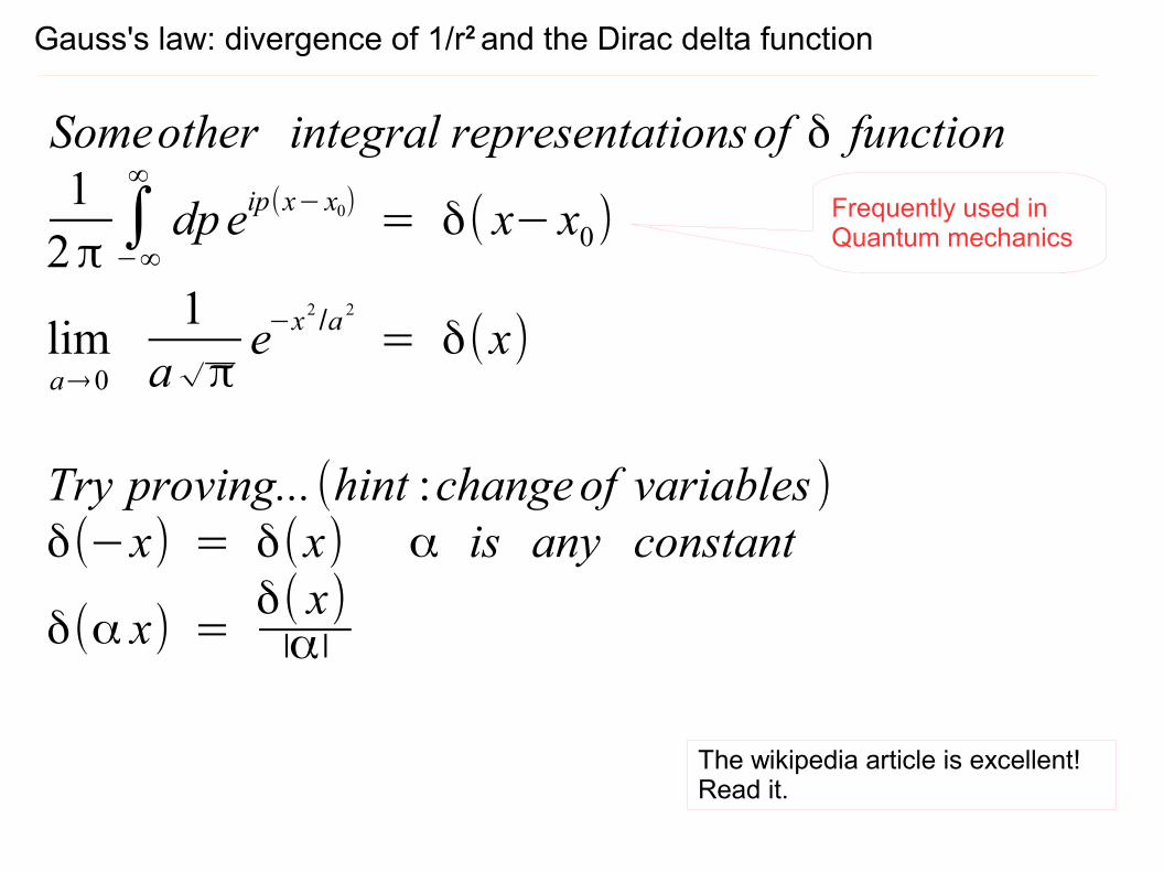
Someother integral representationsof δ function1
2π∫−∞
∞
dpeip(x− x0) = δ( x− x0)
lima→0
1a√π
e−x2/a 2
= δ(x)
Try proving...(hint :changeof variables )δ(−x) = δ(x) α is any constant
δ(α x) =δ( x)∣α∣
Frequently used inQuantum mechanics
The wikipedia article is excellent!Read it.
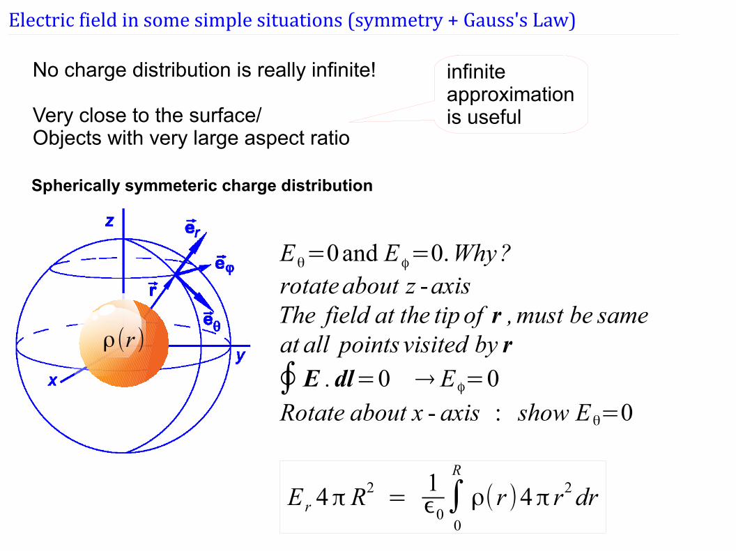
Electric field in some simple situations (symmetry + Gauss's Law)
No charge distribution is really infinite! Very close to the surface/ Objects with very large aspect ratio
infinite approximationis useful
Eθ=0and Eϕ=0.Why?rotateabout z -axisThe field at the tip of r ,must be sameat all points visited by r
∮E .dl=0 → Eϕ=0Rotate about x - axis : show Eθ=0
E r 4π R2=
1ϵ0∫
0
R
ρ(r )4π r2dr
ρ(r )
Spherically symmeteric charge distribution
Electric field in some simple situations (symmetry + Gauss's Law)
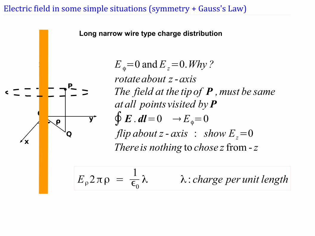
Long narrow wire type charge distribution
E ϕ=0 andE z=0.Why ?rotateabout z -axisThe field at the tipof P ,must be sameat all pointsvisited by P
∮E .dl=0 → Eϕ=0flip about z - axis : show E z=0Thereis nothing to chose z from - z
Eρ2πρ =1ϵ0λ λ : charge per unit length
Electric field in some simple situations (symmetry + Gauss's Law)
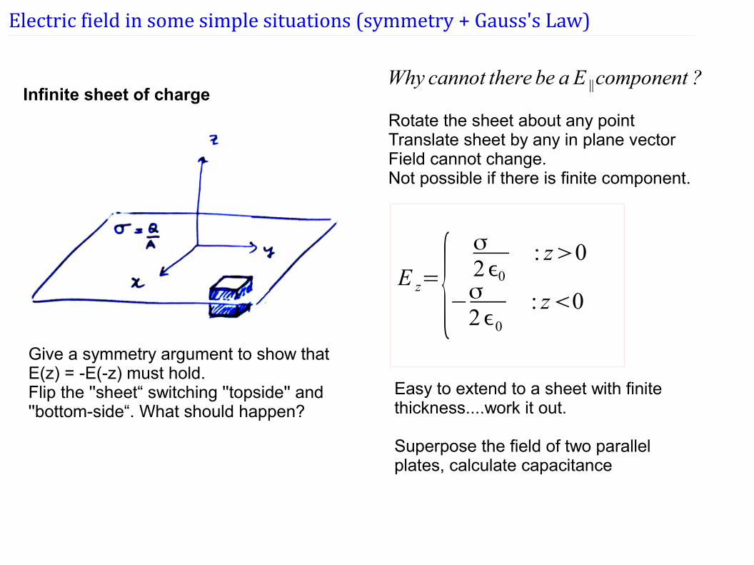
Infinite sheet of charge
Rotate the sheet about any point Translate sheet by any in plane vectorField cannot change. Not possible if there is finite component.
Why cannot there be a E∥component ?
E z={σ2ϵ0
: z>0
−σ2ϵ0
: z<0
Give a symmetry argument to show that E(z) = -E(-z) must hold.Flip the ''sheet“ switching ''topside'' and ''bottom-side“. What should happen?
Easy to extend to a sheet with finite thickness....work it out.
Superpose the field of two parallel plates, calculate capacitance
Some extra charge is placed in a conductor : why does it go to the surface?
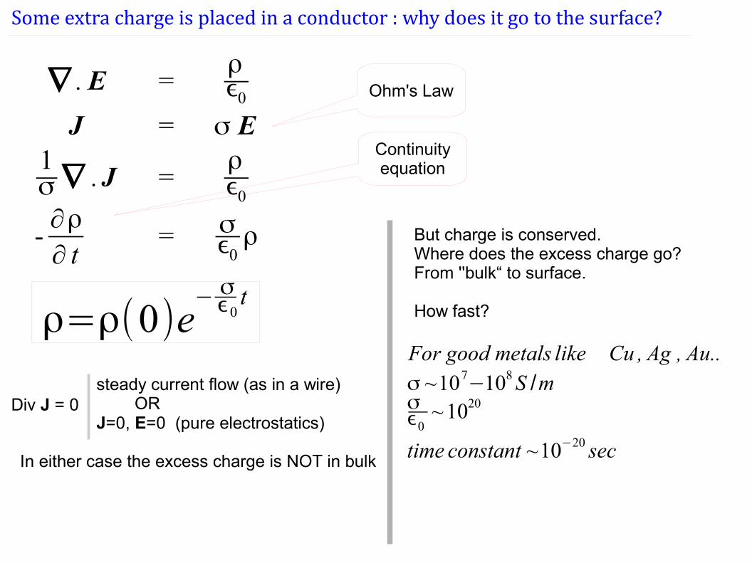
∇ .E =ρϵ0
J = σ E1σ ∇ .J =
ρϵ0
-∂ρ
∂ t= σ
ϵ0ρ
Ohm's Law
Continuityequation
ρ=ρ(0)e− σϵ0t
But charge is conserved. Where does the excess charge go?From ''bulk“ to surface.
How fast?
For good metals like Cu , Ag , Au..σ ~107
−108S /mσϵ0
~ 1020
time constant ~10−20 sec
steady current flow (as in a wire) OR J=0, E=0 (pure electrostatics)
In either case the excess charge is NOT in bulk
Div J = 0
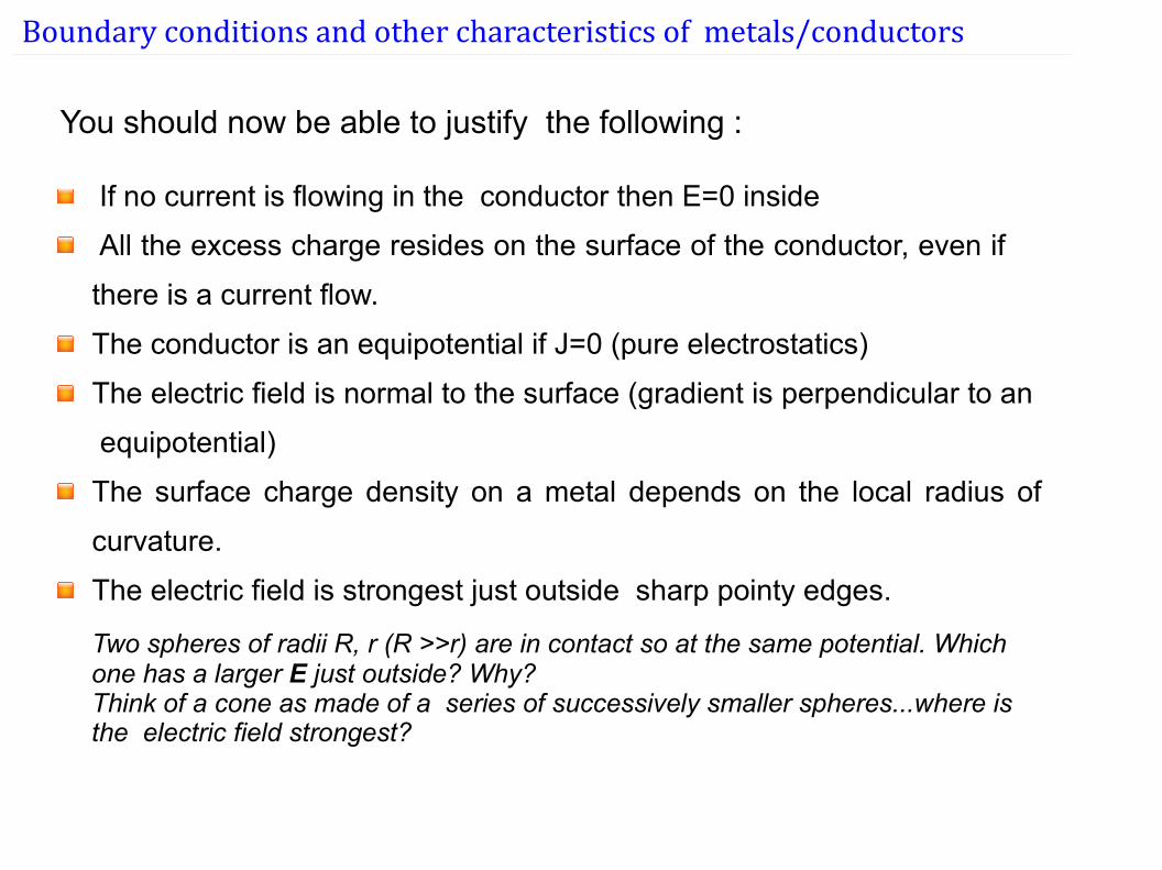
Boundary conditions and other characteristics of metals/conductors
If no current is flowing in the conductor then E=0 inside
All the excess charge resides on the surface of the conductor, even if
there is a current flow.
The conductor is an equipotential if J=0 (pure electrostatics)
The electric field is normal to the surface (gradient is perpendicular to an
equipotential)
The surface charge density on a metal depends on the local radius of
curvature.
The electric field is strongest just outside sharp pointy edges.
You should now be able to justify the following :
Two spheres of radii R, r (R >>r) are in contact so at the same potential. Which one has a larger E just outside? Why?Think of a cone as made of a series of successively smaller spheres...where is the electric field strongest?
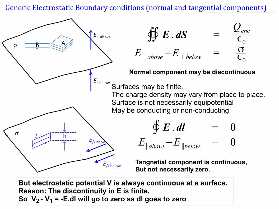
Generic Electrostatic Boundary conditions (normal and tangential components)
∯ E .dS =Qencϵ0
E ⊥above−E ⊥below = σϵ0
∮E .dl = 0E∥above−E∥below = 0
h AE above
Ebelow
E// below
hl E// above
Surfaces may be finite. The charge density may vary from place to place.Surface is not necessarily equipotentialMay be conducting or non-conducting
Normal component may be discontinuous
Tangnetial component is continuous,But not necessarily zero.
But electrostatic potential V is always continuous at a surface.Reason: The discontinuity in E is finite. So V2 - V1 = -E.dl will go to zero as dl goes to zero
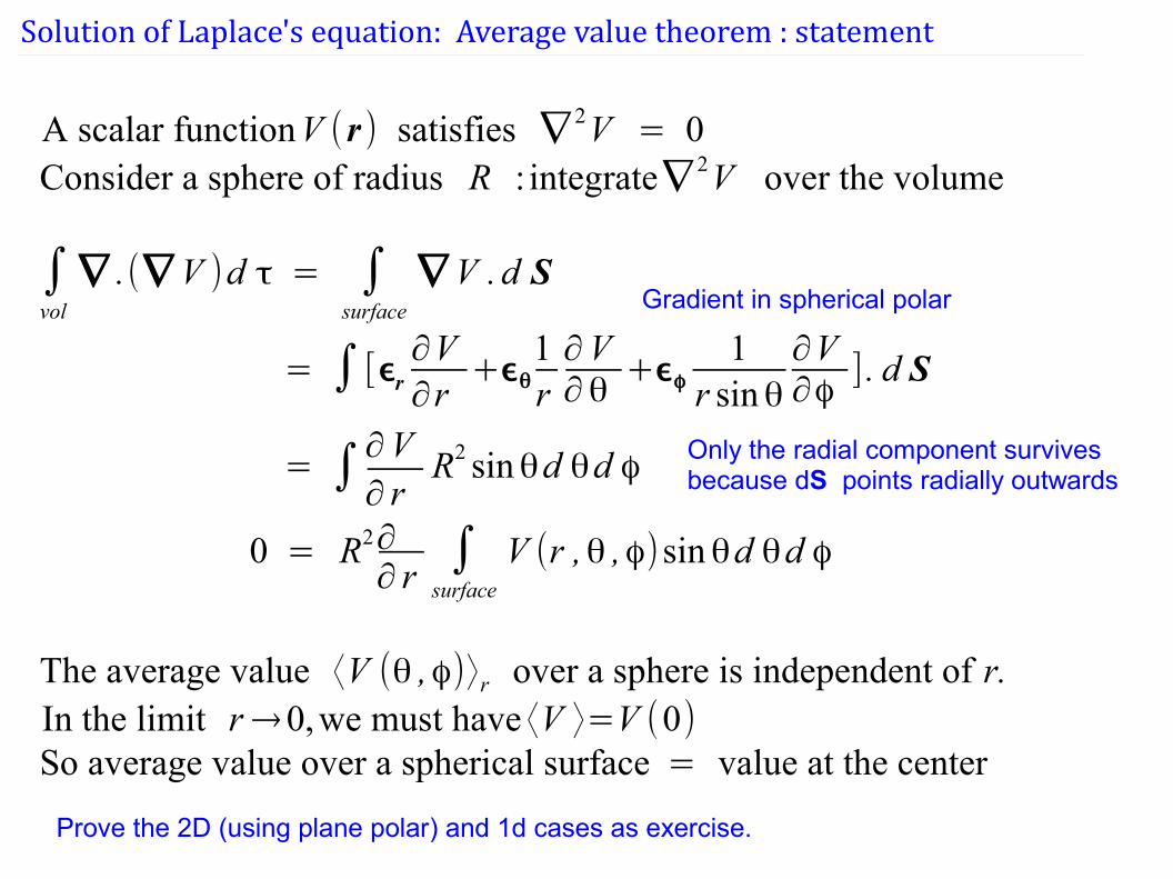
Solution of Laplace's equation: Average value theorem : statement
A scalar functionV (r ) satisfies ∇2V = 0
Consider a sphere of radius R : integrate∇ 2V over the volume
∫vol
∇ .(∇ V )d τ = ∫surface
∇ V .d S
= ∫ [ϵr∂V∂r
+ϵθ1r∂V∂θ
+ϵϕ1
r sinθ∂V∂ϕ
] . d S
= ∫∂V∂ r
R2 sinθd θd ϕ
0 = R2∂∂ r∫
surface
V (r ,θ ,ϕ)sinθd θd ϕ
The average value ⟨V (θ ,ϕ)⟩r over a sphere is independent of r.In the limit r→0,we must have ⟨V ⟩=V (0)So average value over a spherical surface = value at the center
Gradient in spherical polar
Only the radial component survives because dS points radially outwards
Prove the 2D (using plane polar) and 1d cases as exercise.
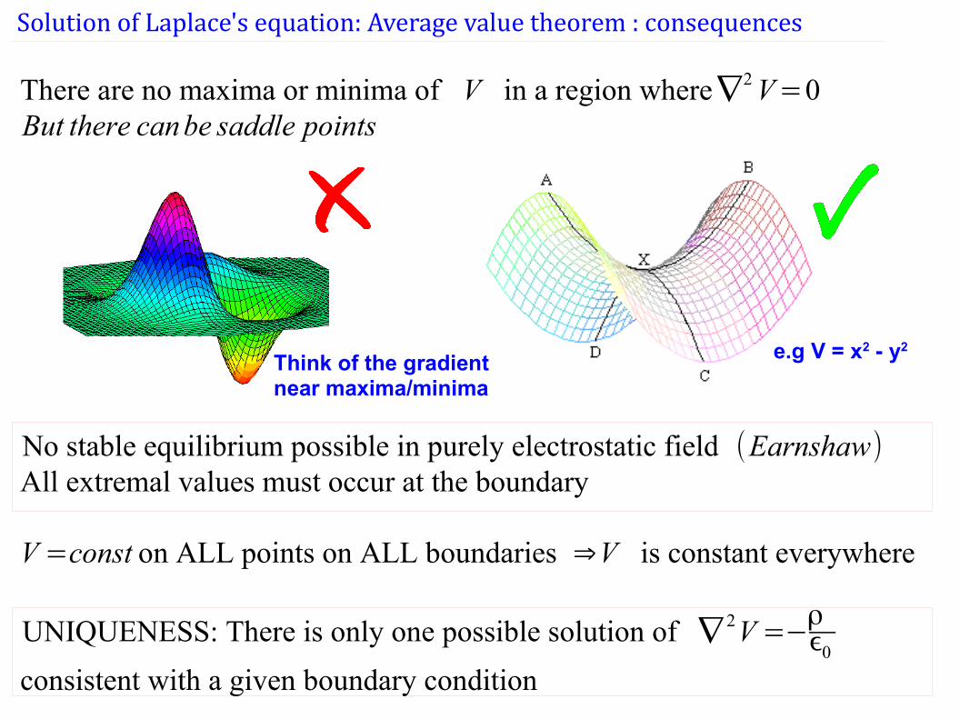
There are no maxima or minima of V in a region where∇2V=0But there canbe saddle points
No stable equilibrium possible in purely electrostatic field (Earnshaw)All extremal values must occur at the boundary
V=const on ALL points on ALL boundaries ⇒V is constant everywhere
UNIQUENESS: There is only one possible solution of ∇ 2V=−ρϵ0
consistent with a given boundary condition
Solution of Laplace's equation: Average value theorem : consequences
e.g V = x2 - y2
Think of the gradient near maxima/minima
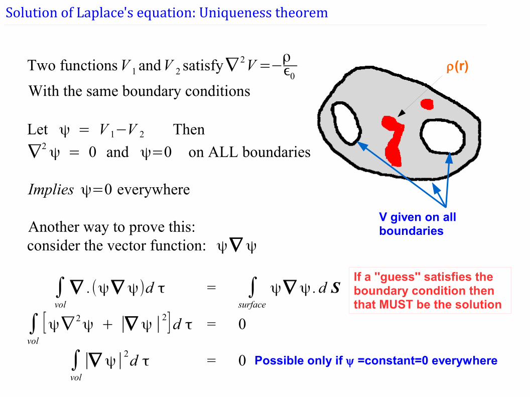
Solution of Laplace's equation: Uniqueness theorem
Two functionsV 1 andV 2 satisfy∇ 2V=−ρϵ0
With the same boundary conditions
Let ψ = V 1−V 2 Then
∇2ψ = 0 and ψ=0 on ALL boundaries
Implies ψ=0 everywhere
Another way to prove this:consider the vector function: ψ∇ ψ
∫vol
∇ .(ψ∇ ψ)d τ = ∫surface
ψ∇ ψ . d S
∫vol
[ψ∇ 2ψ + ∣∇ ψ ∣
2]d τ = 0
∫vol
∣∇ ψ∣2d τ = 0
V given on all boundaries
r(r)
Possible only if y =constant=0 everywhere
If a ''guess'' satisfies the boundary condition then that MUST be the solution
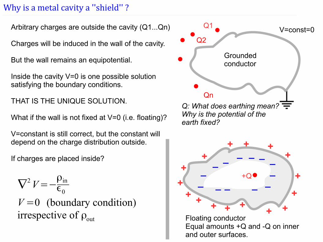
Why is a metal cavity a ''shield'' ?
V=const=0Q1
Q2
Arbitrary charges are outside the cavity (Q1...Qn)
Charges will be induced in the wall of the cavity.
But the wall remains an equipotential.
Inside the cavity V=0 is one possible solution satisfying the boundary conditions.
THAT IS THE UNIQUE SOLUTION.
What if the wall is not fixed at V=0 (i.e. floating)?
V=constant is still correct, but the constant willdepend on the charge distribution outside.
If charges are placed inside?
Qn
Q: What does earthing mean?Why is the potential of the earth fixed?
∇2V=−
ρinϵ0
V=0 (boundary condition)irrespective of ρout
+Q
_ _____ _
_
___ __
+
+
++
+
+
+++++
++
+
++
Grounded conductor
Floating conductorEqual amounts +Q and -Q on inner and outer surfaces.
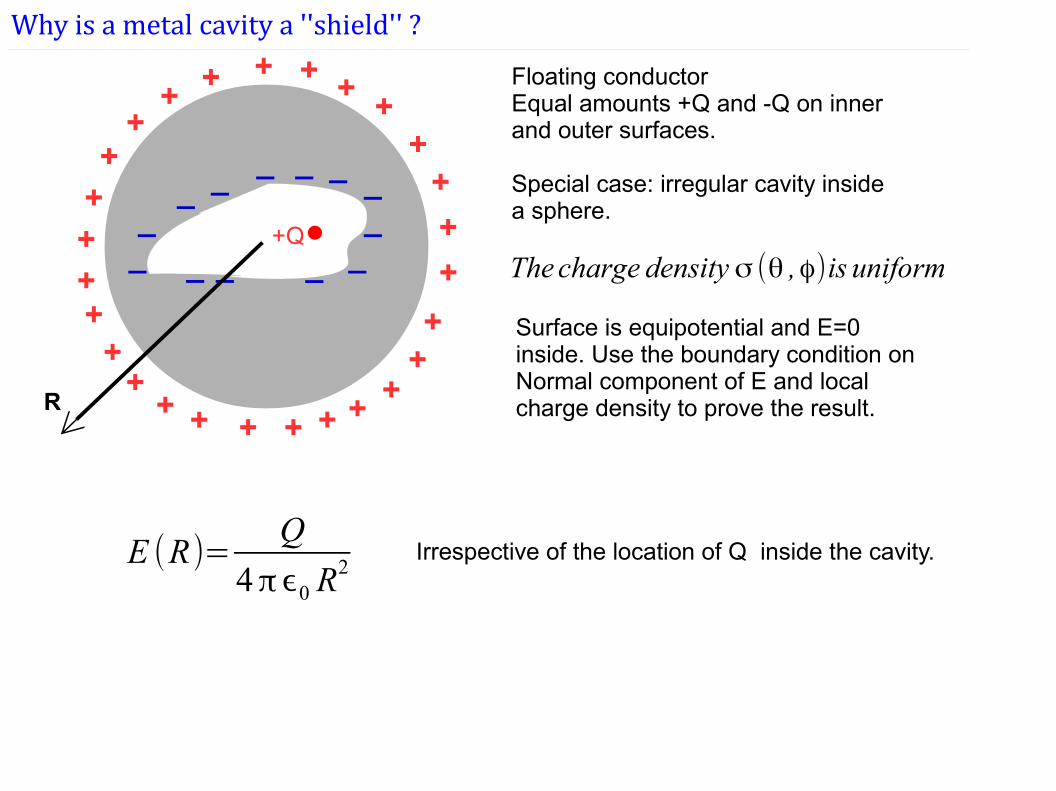
Why is a metal cavity a ''shield'' ?
+ Floating conductorEqual amounts +Q and -Q on inner and outer surfaces.
Special case: irregular cavity inside a sphere.
+Q
_ _____ _
_
___ __
++
+
+
+
++
+++++++
++
+++++
++
+ + +
Thecharge density σ (θ ,ϕ)is uniform
Surface is equipotential and E=0 inside. Use the boundary condition onNormal component of E and local charge density to prove the result. R
E (R)=Q
4πϵ0 R2
Irrespective of the location of Q inside the cavity.
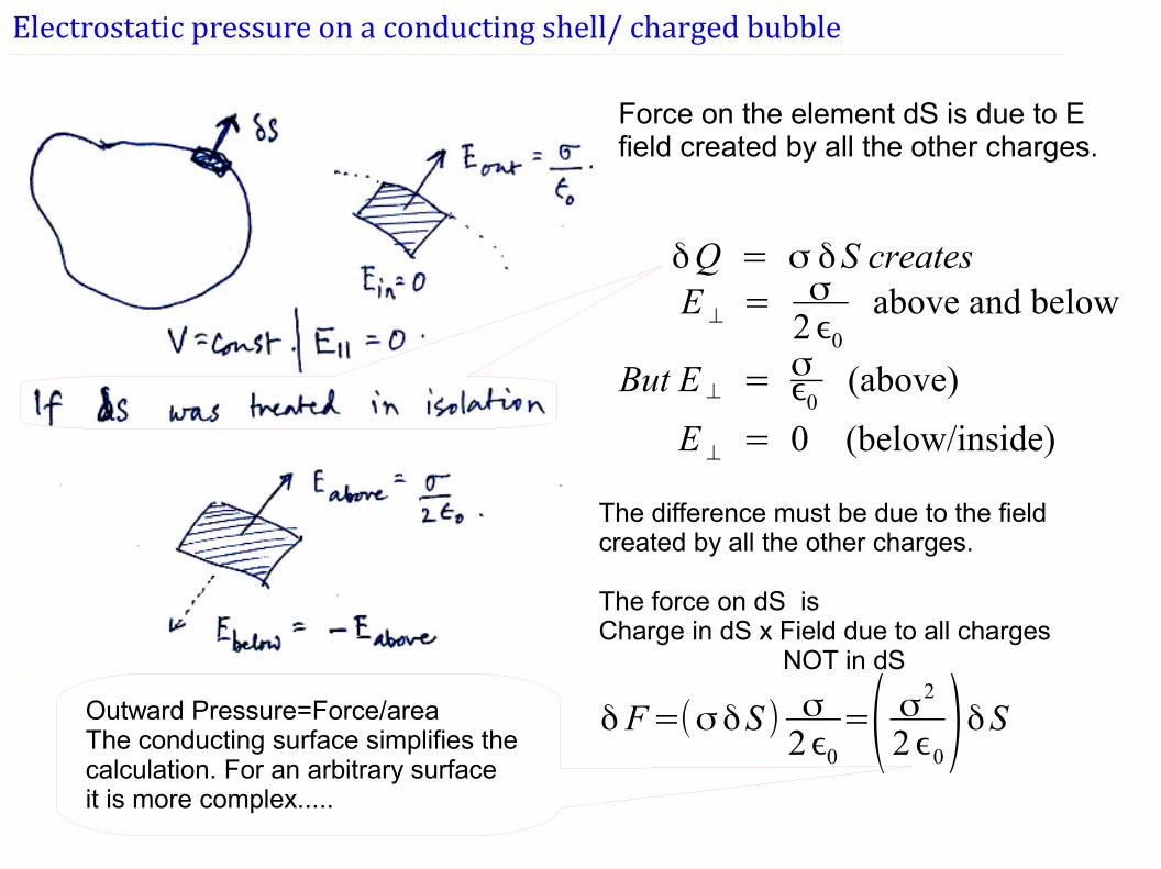
Electrostatic pressure on a conducting shell/ charged bubble
Force on the element dS is due to E field created by all the other charges.
δQ = σ δS createsE ⊥ =
σ2ϵ0
above and below
But E ⊥ = σϵ0
(above)
E ⊥ = 0 (below/inside)
The difference must be due to the field created by all the other charges.
The force on dS isCharge in dS x Field due to all charges NOT in dS
δ F=(σδS ) σ2ϵ0
=( σ2
2ϵ0)δSOutward Pressure=Force/areaThe conducting surface simplifies the calculation. For an arbitrary surfaceit is more complex.....
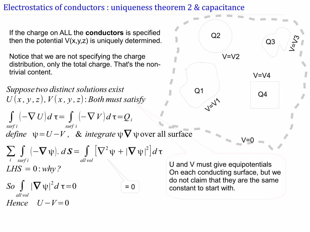
Electrostatics of conductors : uniqueness theorem 2 & capacitance
V=V
3
If the charge on ALL the conductors is specified then the potential V(x,y,z) is uniquely determined.
Notice that we are not specifying the charge distribution, only the total charge. That's the non-trivial content.
Suppose two distinct solutions existU (x , y , z ) ,V ( x , y , z) :Both must satisfy
∫surf i
(−∇U )d τ= ∫surf i
(−∇ V )d τ=Q i
define ψ=U−V , & integrate ψ∇ ψover all surface
∑i∫surf i
(−∇ ψ) . d S= ∫all vol
[∇ 2ψ + |∇ ψ |2 ]d τ
LHS = 0 :why?
So ∫all vol
|∇ ψ |2d τ=0
Hence U−V=0
Q1
V=V1
Q2Q3
Q4
V=V2
V=V4
V=0
U and V must give equipotentialsOn each conducting surface, but we do not claim that they are the same constant to start with. = 0
Electrostatics of conductors : uniqueness theorem 2 & capacitance
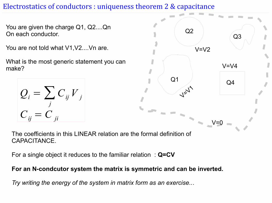
You are given the charge Q1, Q2....QnOn each conductor.
You are not told what V1,V2....Vn are.
What is the most generic statement you can make?
Q1
V=V1
Q2Q3
Q4
V=V2
V=V4
V=0
Qi =∑j
C ijV j
C ij= C ji
The coefficients in this LINEAR relation are the formal definition of CAPACITANCE.
For a single object it reduces to the familiar relation : Q=CV
For an N-condcutor system the matrix is symmetric and can be inverted.
Try writing the energy of the system in matrix form as an exercise...
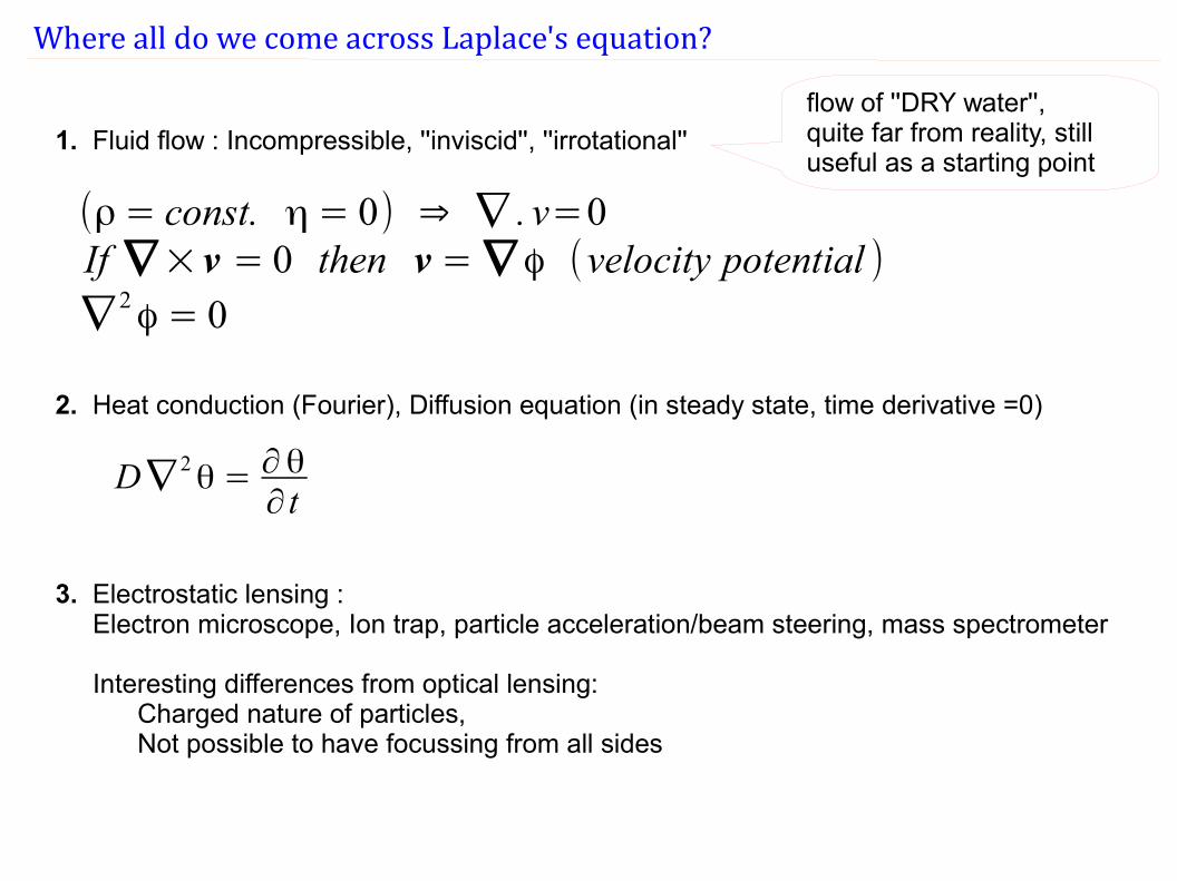
Where all do we come across Laplace's equation?
1. Fluid flow : Incompressible, ''inviscid'', ''irrotational''
(ρ = const. η = 0) ⇒ ∇ . v=0If ∇× v = 0 then v = ∇ϕ (velocity potential )∇
2ϕ = 0
flow of ''DRY water'', quite far from reality, still useful as a starting point
2. Heat conduction (Fourier), Diffusion equation (in steady state, time derivative =0)
D∇ 2θ = ∂θ
∂ t
3. Electrostatic lensing : Electron microscope, Ion trap, particle acceleration/beam steering, mass spectrometer Interesting differences from optical lensing: Charged nature of particles, Not possible to have focussing from all sides
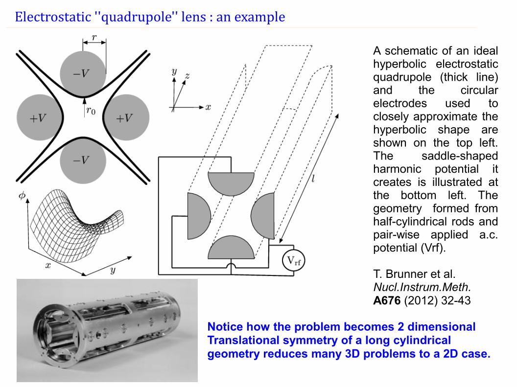
Electrostatic ''quadrupole'' lens : an example
A schematic of an ideal hyperbolic electrostatic quadrupole (thick line) and the circular electrodes used to closely approximate the hyperbolic shape are shown on the top left. The saddle-shaped harmonic potential it creates is illustrated at the bottom left. The geometry formed from half-cylindrical rods and pair-wise applied a.c. potential (Vrf).
T. Brunner et al. Nucl.Instrum.Meth. A676 (2012) 32-43
Notice how the problem becomes 2 dimensionalTranslational symmetry of a long cylindrical geometry reduces many 3D problems to a 2D case.
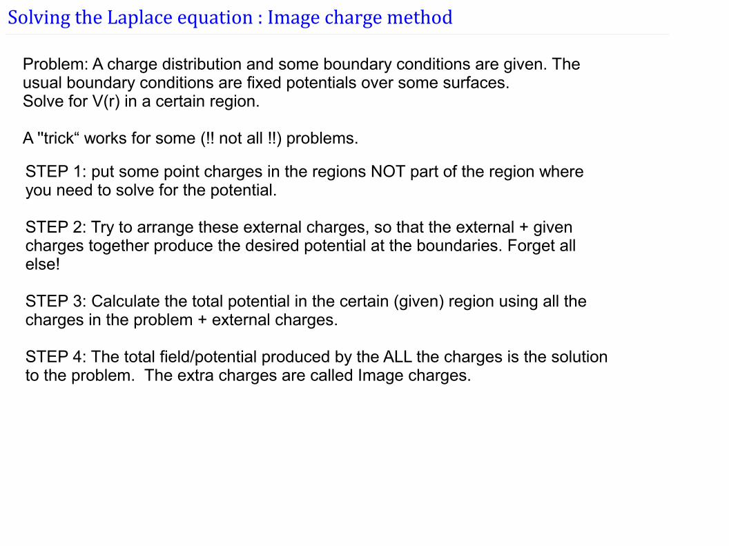
Solving the Laplace equation : Image charge method
Problem: A charge distribution and some boundary conditions are given. The usual boundary conditions are fixed potentials over some surfaces.Solve for V(r) in a certain region.
A ''trick“ works for some (!! not all !!) problems.
STEP 1: put some point charges in the regions NOT part of the region where you need to solve for the potential.
STEP 2: Try to arrange these external charges, so that the external + given charges together produce the desired potential at the boundaries. Forget all else!
STEP 3: Calculate the total potential in the certain (given) region using all the charges in the problem + external charges.
STEP 4: The total field/potential produced by the ALL the charges is the solution to the problem. The extra charges are called Image charges.
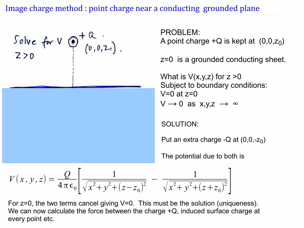
Image charge method : point charge near a conducting grounded plane
PROBLEM:A point charge +Q is kept at (0,0,z0)
z=0 is a grounded conducting sheet.
What is V(x,y,z) for z >0 Subject to boundary conditions:V=0 at z=0V → 0 as x,y,z → ∞
SOLUTION:
Put an extra charge -Q at (0,0,-z0)
The potential due to both is
V ( x , y , z) =Q
4πϵ0 [ 1
√ x2+ y2
+(z−z0)2−
1
√ x2+ y2
+(z+z0)2 ]
For z=0, the two terms cancel giving V=0. This must be the solution (uniqueness).We can now calculate the force between the charge +Q, induced surface charge at every point etc.
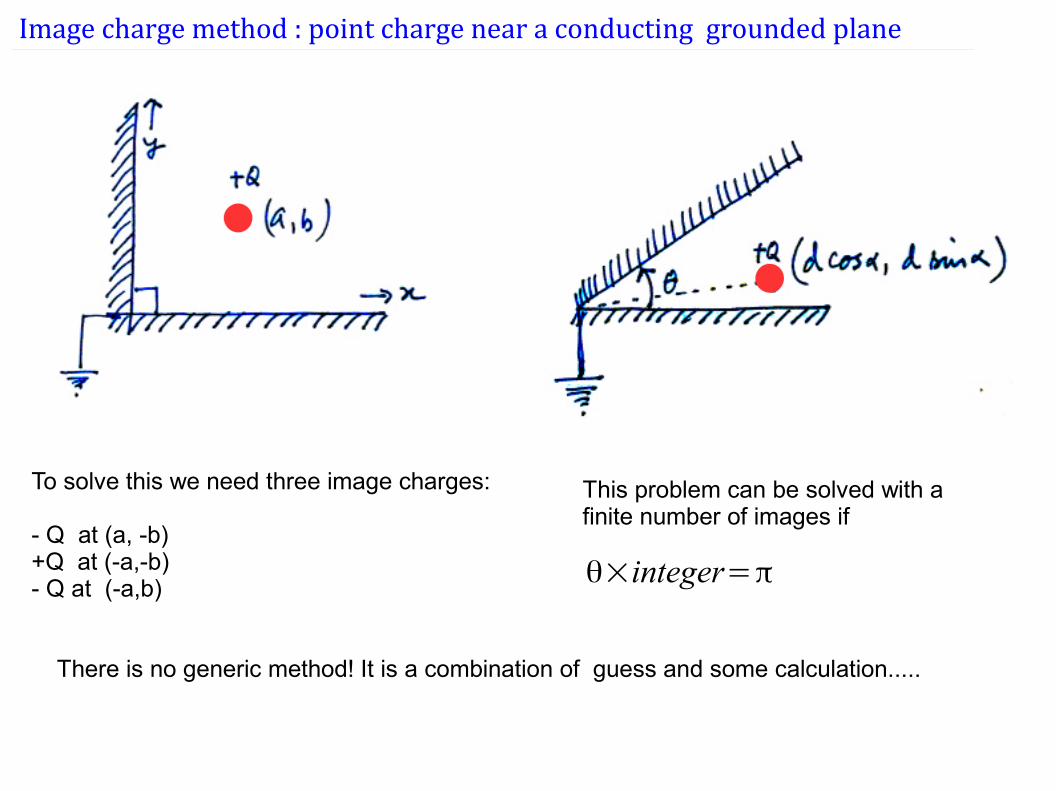
Image charge method : point charge near a conducting grounded plane
To solve this we need three image charges:
- Q at (a, -b)+Q at (-a,-b)- Q at (-a,b)
This problem can be solved with a finite number of images if
θ×integer=π
There is no generic method! It is a combination of guess and some calculation.....
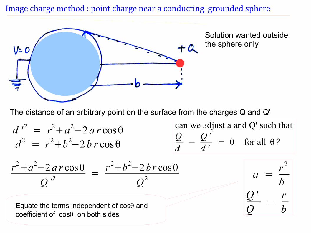
Image charge method : point charge near a conducting grounded sphere
Solution wanted outside the sphere only
d ' 2 = r2+a2
−2a r cosθd 2 = r 2+b2−2b r cosθ
The distance of an arbitrary point on the surface from the charges Q and Q'
can we adjust a and Q' such thatQd
−Q 'd '
= 0 for all θ?
r2+a2
−2a r cosθ
Q ' 2=
r 2+b2
−2br cosθ
Q 2 a =r 2
bQ 'Q
=rbEquate the terms independent of cosq and
coefficient of cosq on both sides
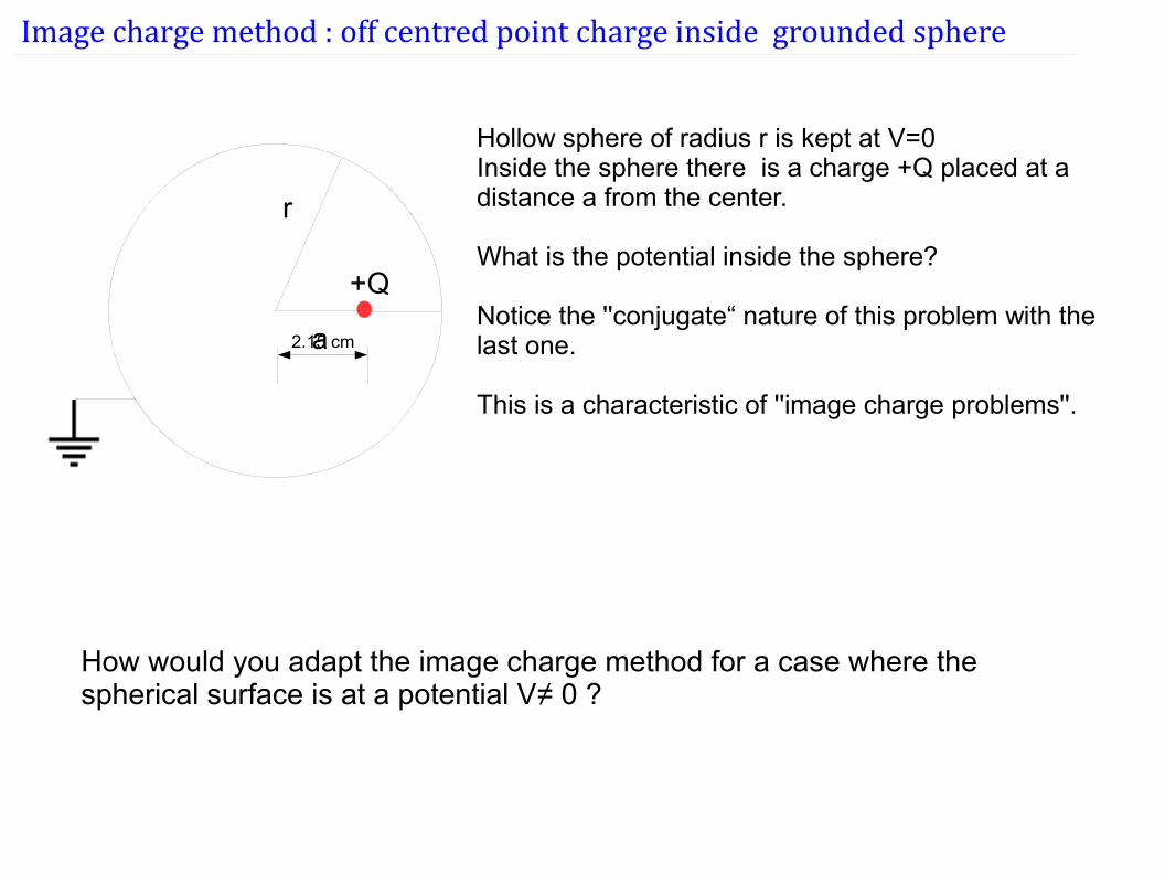
Image charge method : off centred point charge inside grounded sphere
r
a
Hollow sphere of radius r is kept at V=0Inside the sphere there is a charge +Q placed at a distance a from the center.
What is the potential inside the sphere?
Notice the ''conjugate“ nature of this problem with the last one.
This is a characteristic of ''image charge problems''.
+Q
2.15 cm
How would you adapt the image charge method for a case where the spherical surface is at a potential V≠ 0 ?
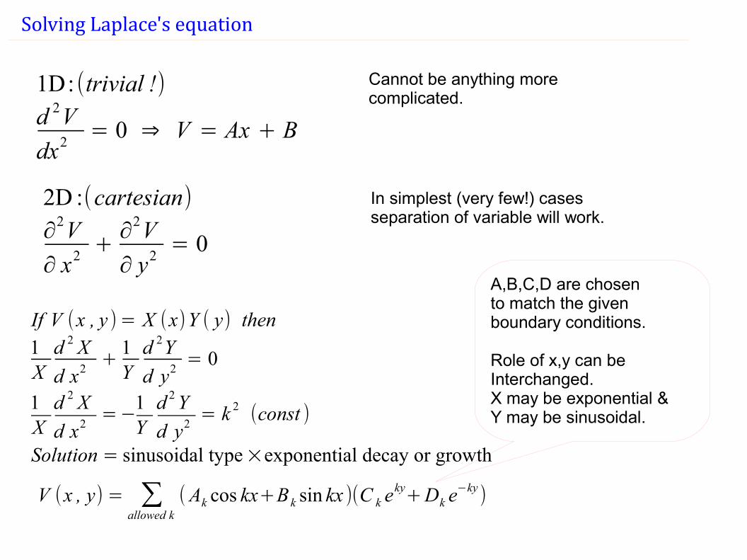
Solving Laplace's equation
1D:(trivial !)d 2V
dx2= 0 ⇒ V = Ax + B
Cannot be anything more complicated.
2D :(cartesian)∂
2V
∂ x2+∂
2V
∂ y2= 0
In simplest (very few!) cases separation of variable will work.
If V (x , y )= X (x)Y ( y) then1Xd 2 X
d x2+
1Yd 2Y
d y2= 0
1Xd 2 X
d x2=−
1Yd 2Y
d y2= k 2
(const )
Solution = sinusoidal type×exponential decay or growth
V (x , y) = ∑allowed k
(Ak cos kx+B k sin kx )(C k eky+Dk e
−ky)
A,B,C,D are chosen to match the given boundary conditions.
Role of x,y can be Interchanged. X may be exponential & Y may be sinusoidal.
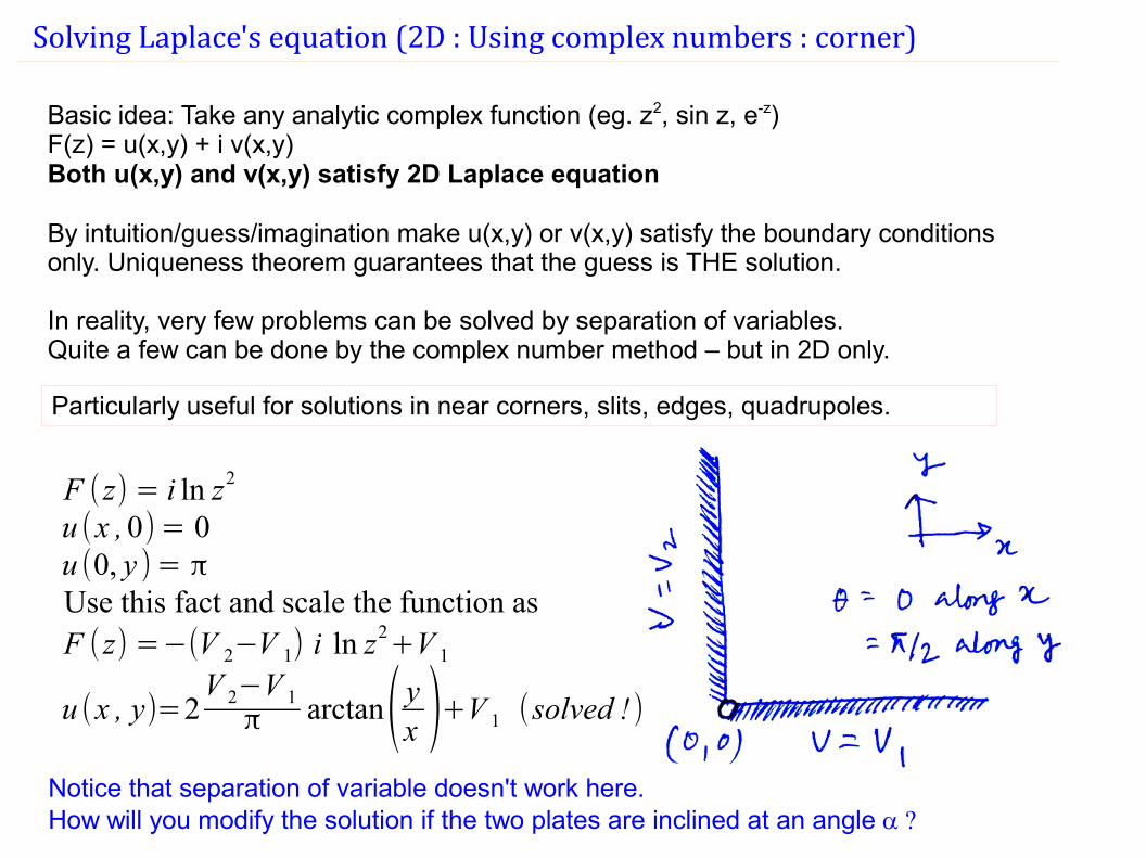
Solving Laplace's equation (2D : Using complex numbers : corner)
Basic idea: Take any analytic complex function (eg. z2, sin z, e-z)F(z) = u(x,y) + i v(x,y)Both u(x,y) and v(x,y) satisfy 2D Laplace equation
By intuition/guess/imagination make u(x,y) or v(x,y) satisfy the boundary conditions only. Uniqueness theorem guarantees that the guess is THE solution.
In reality, very few problems can be solved by separation of variables. Quite a few can be done by the complex number method – but in 2D only.
F (z) = i ln z2
u (x ,0)= 0u (0, y )= πUse this fact and scale the function asF (z) =−(V 2−V 1) i ln z2
+V 1
u (x , y)=2V 2−V 1π arctan( yx )+V 1 (solved ! )
Notice that separation of variable doesn't work here.How will you modify the solution if the two plates are inclined at an angle a ?
Particularly useful for solutions in near corners, slits, edges, quadrupoles.
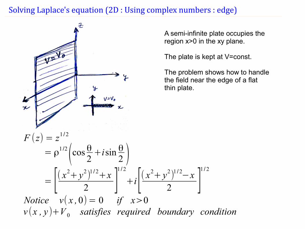
Solving Laplace's equation (2D : Using complex numbers : edge)
F (z) = z1 /2
= ρ1 /2(cos θ2+isin θ
2 )= [( x
2+ y2)1 /2+x2 ]
1 /2
+i[( x2+ y2)1 /2−x
2 ]1 /2
Notice v( x ,0)= 0 if x>0v (x , y )+V 0 satisfies required boundary condition
A semi-infinite plate occupies the region x>0 in the xy plane.
The plate is kept at V=const.
The problem shows how to handle the field near the edge of a flat thin plate.
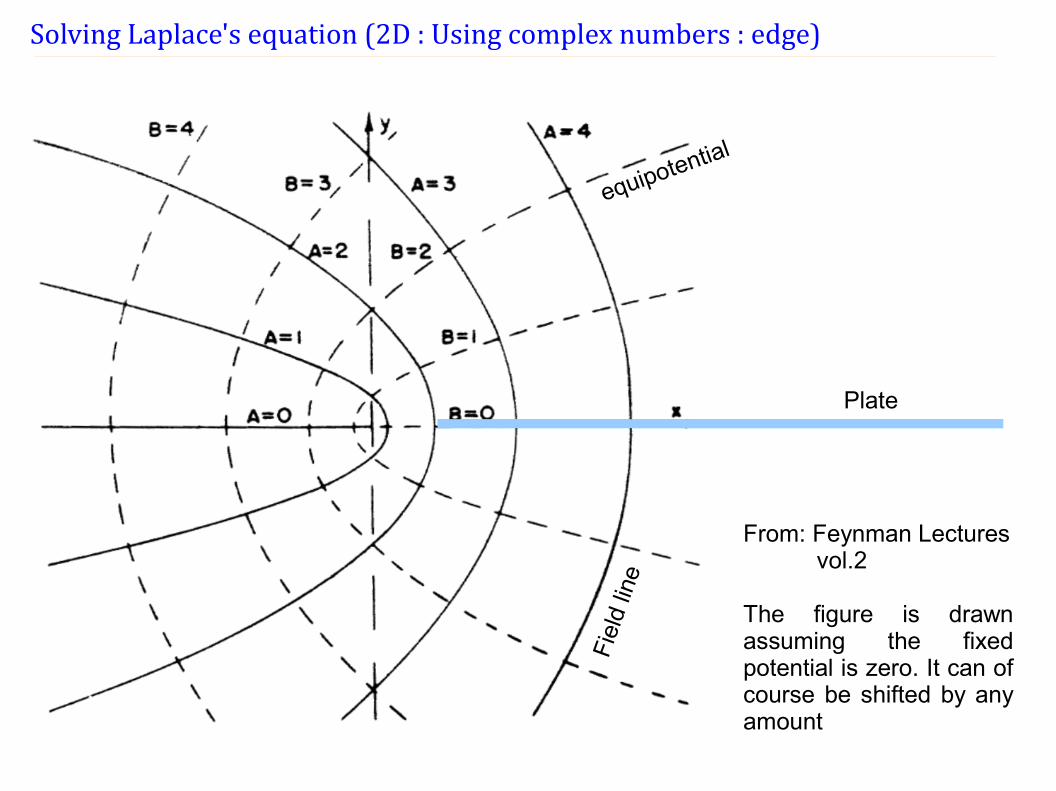
Solving Laplace's equation (2D : Using complex numbers : edge)
Plate
equipotential
Fie
ld li
ne
From: Feynman Lectures vol.2
The figure is drawn assuming the fixed potential is zero. It can of course be shifted by any amount
Solving Laplace's equation (2D : Using complex numbers : slit)
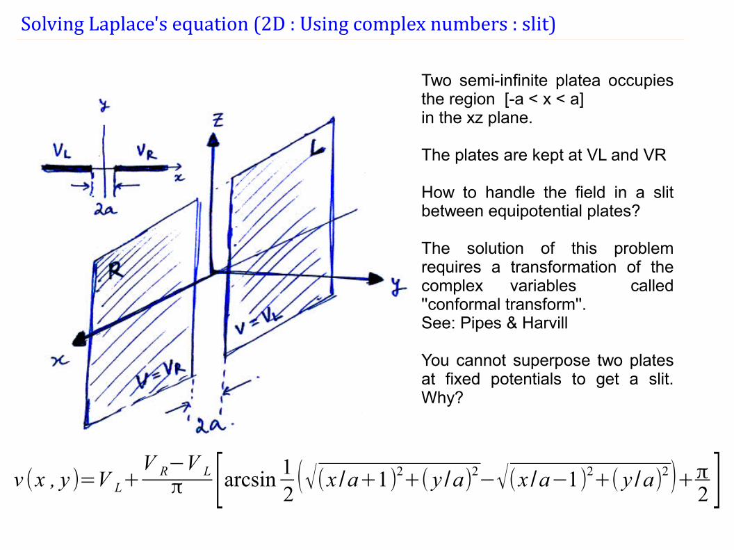
Two semi-infinite platea occupies the region [-a < x < a] in the xz plane.
The plates are kept at VL and VR How to handle the field in a slit between equipotential plates?
The solution of this problem requires a transformation of the complex variables called ''conformal transform''.See: Pipes & Harvill
You cannot superpose two plates at fixed potentials to get a slit. Why?
v (x , y )=V L+V R−V Lπ [arcsin
12(√(x /a+1)2+( y /a)2−√(x /a−1)2+( y /a)2)+π
2 ]
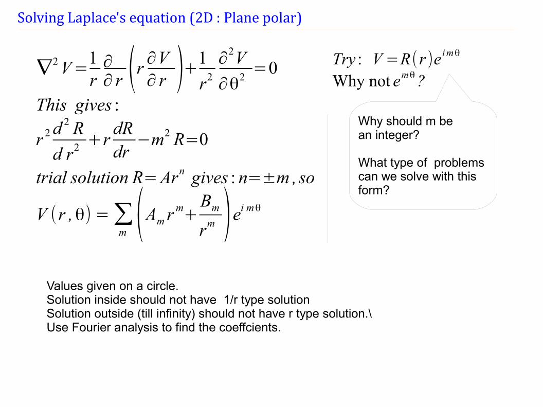
Solving Laplace's equation (2D : Plane polar)
∇2V=
1r∂∂ r (r ∂V∂ r )+1
r2
∂2V
∂θ2=0
This gives :
r 2d2 R
d r2 +rdRdr−m2 R=0
trial solution R=Arn gives : n=±m ,so
V (r ,θ) =∑m (Am r
m+Bm
rm )ei mθ
Try : V=R(r )e imθ
Why not emθ?
Why should m be an integer?
What type of problems can we solve with this form?
Values given on a circle. Solution inside should not have 1/r type solutionSolution outside (till infinity) should not have r type solution.\Use Fourier analysis to find the coeffcients.
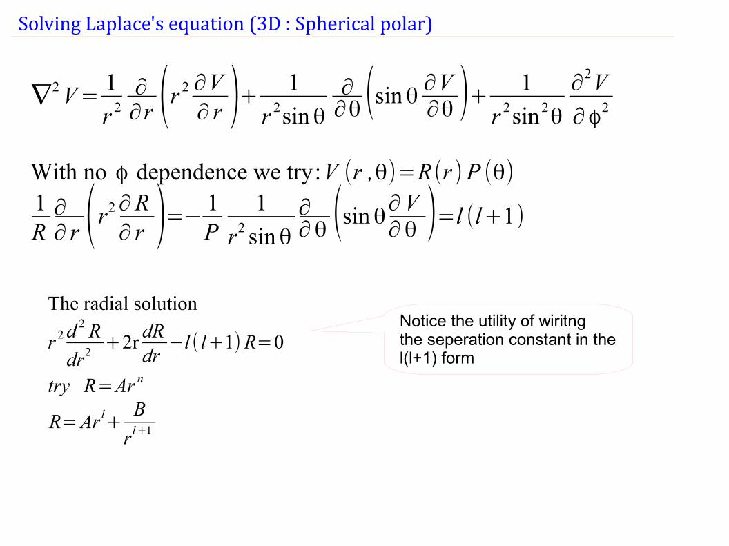
Solving Laplace's equation (3D : Spherical polar)
∇2V=
1
r 2∂∂r (r 2 ∂V
∂ r )+ 1
r 2sinθ∂∂θ (sinθ
∂V∂θ )+
1
r 2sin2θ
∂2V
∂ϕ2
With no ϕ dependence we try:V (r ,θ)=R(r )P (θ)1R∂∂ r (r2∂R
∂ r )=− 1P
1
r2 sinθ∂∂θ (sinθ
∂V∂ θ )=l (l+1)
The radial solution
r 2d2 R
dr2+2r
dRdr−l ( l+1)R=0
try R=Ar n
R=Ar l+B
r l+1
Notice the utility of wiritng the seperation constant in thel(l+1) form
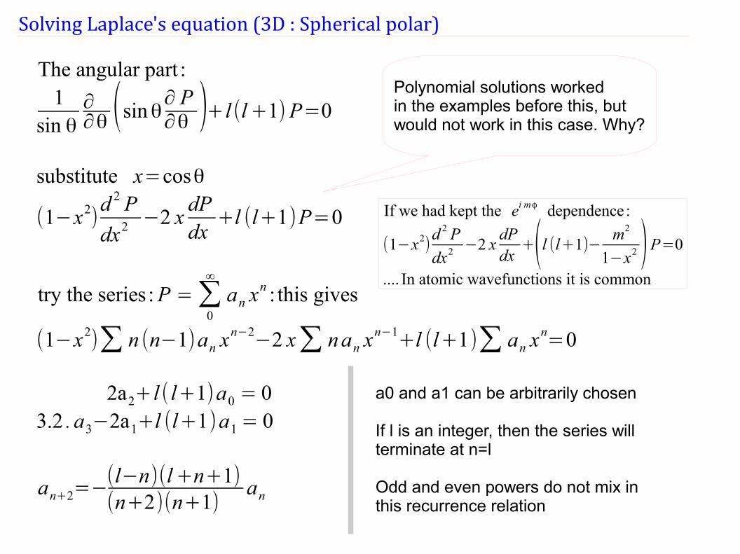
Solving Laplace's equation (3D : Spherical polar)
The angular part :1
sin θ∂∂θ (sinθ
∂ P∂θ )+ l (l+1)P=0
substitute x=cosθ
(1−x2)d 2 P
dx2 −2 xdPdx
+l (l+1)P=0
try the series :P =∑0
∞
an xn : this gives
(1−x2)∑ n (n−1)an x
n−2−2 x∑ nan x
n−1+l (l+1)∑ an x
n=0
2a2+ l ( l+1)a0 = 03.2 . a3−2a1+l (l+1)a1= 0
an+2=−(l−n)(l+n+1)(n+2)(n+1)
an
Polynomial solutions worked in the examples before this, butwould not work in this case. Why?
a0 and a1 can be arbitrarily chosen
If l is an integer, then the series will terminate at n=l
Odd and even powers do not mix in this recurrence relation
If we had kept the ei mϕ dependence :
(1−x2)d 2 P
dx2 −2 xdPdx
+(l (l+1)−m2
1−x2 )P=0
.... In atomic wavefunctions it is common
Solving Laplace's equation (3D : Spherical polar)
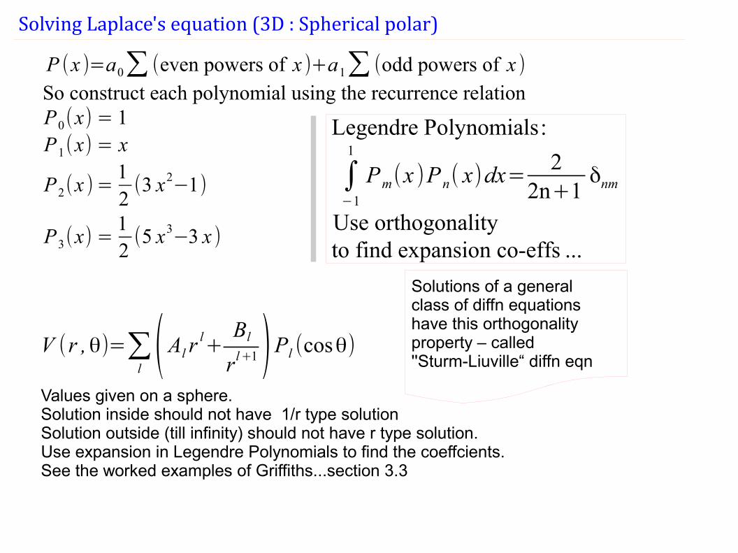
P (x )=a0∑ (even powers of x )+a1∑ (odd powers of x )So construct each polynomial using the recurrence relationP0(x) = 1P1(x) = x
P2(x )=12(3 x2
−1)
P3(x) =12(5 x3
−3 x )
Legendre Polynomials:
∫−1
1
Pm(x )Pn( x)dx=2
2n+1δnm
Use orthogonalityto find expansion co-effs ...
V (r ,θ)=∑l (Al r
l+
Bl
rl+1)Pl (cosθ)
Values given on a sphere. Solution inside should not have 1/r type solutionSolution outside (till infinity) should not have r type solution.Use expansion in Legendre Polynomials to find the coeffcients.See the worked examples of Griffiths...section 3.3
Solutions of a general class of diffn equations have this orthogonality property – called ''Sturm-Liuville“ diffn eqn
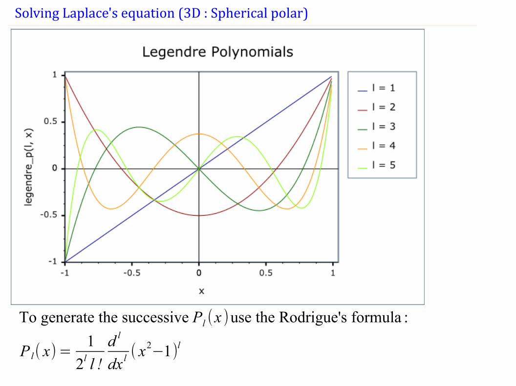
Solving Laplace's equation (3D : Spherical polar)
To generate the successive Pl (x )use the Rodrigue's formula :
P l( x)=1
2l l !
d l
dx l( x2−1)l
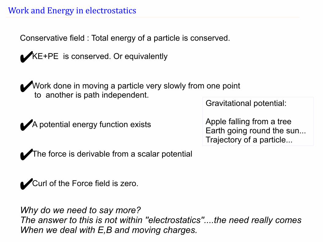
Work and Energy in electrostatics
Conservative field : Total energy of a particle is conserved.
✔KE+PE is conserved. Or equivalently
✔Work done in moving a particle very slowly from one point to another is path independent.
✔A potential energy function exists
✔The force is derivable from a scalar potential
✔Curl of the Force field is zero.
Why do we need to say more? The answer to this is not within ''electrostatics''....the need really comesWhen we deal with E,B and moving charges.
Gravitational potential:
Apple falling from a treeEarth going round the sun...Trajectory of a particle...
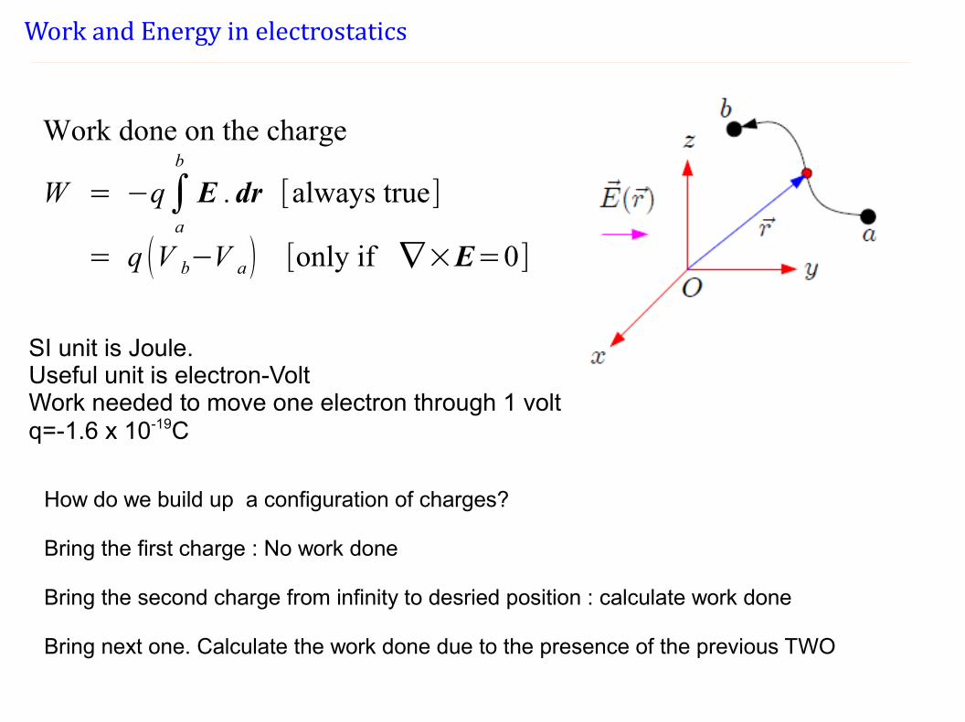
Work and Energy in electrostatics
Work done on the charge
W = −q∫a
b
E .dr [always true]
= q (V b−V a) [only if ∇×E=0]
SI unit is Joule. Useful unit is electron-VoltWork needed to move one electron through 1 voltq=-1.6 x 10⁻¹⁹C
How do we build up a configuration of charges?
Bring the first charge : No work done
Bring the second charge from infinity to desried position : calculate work done
Bring next one. Calculate the work done due to the presence of the previous TWO
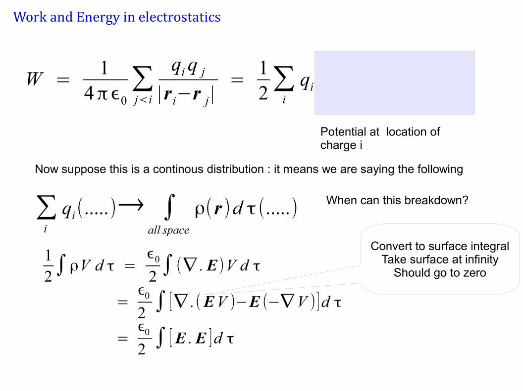
Work and Energy in electrostatics
W =1
4πϵ0∑j<i
qiq j
|r i−r j |=
12∑i
qi1
4πϵ0∑j
q j
|r i−r j |
Potential at location of charge i
Now suppose this is a continous distribution : it means we are saying the following
∑i
qi(.....)→ ∫all space
ρ(r )d τ (.....) When can this breakdown?
12∫ρV d τ =
ϵ0
2∫(∇ .E)V d τ
=ϵ0
2∫ [∇ .(EV )−E (−∇ V )]d τ
=ϵ0
2∫ [E .E ]d τ
Convert to surface integralTake surface at infinity
Should go to zero
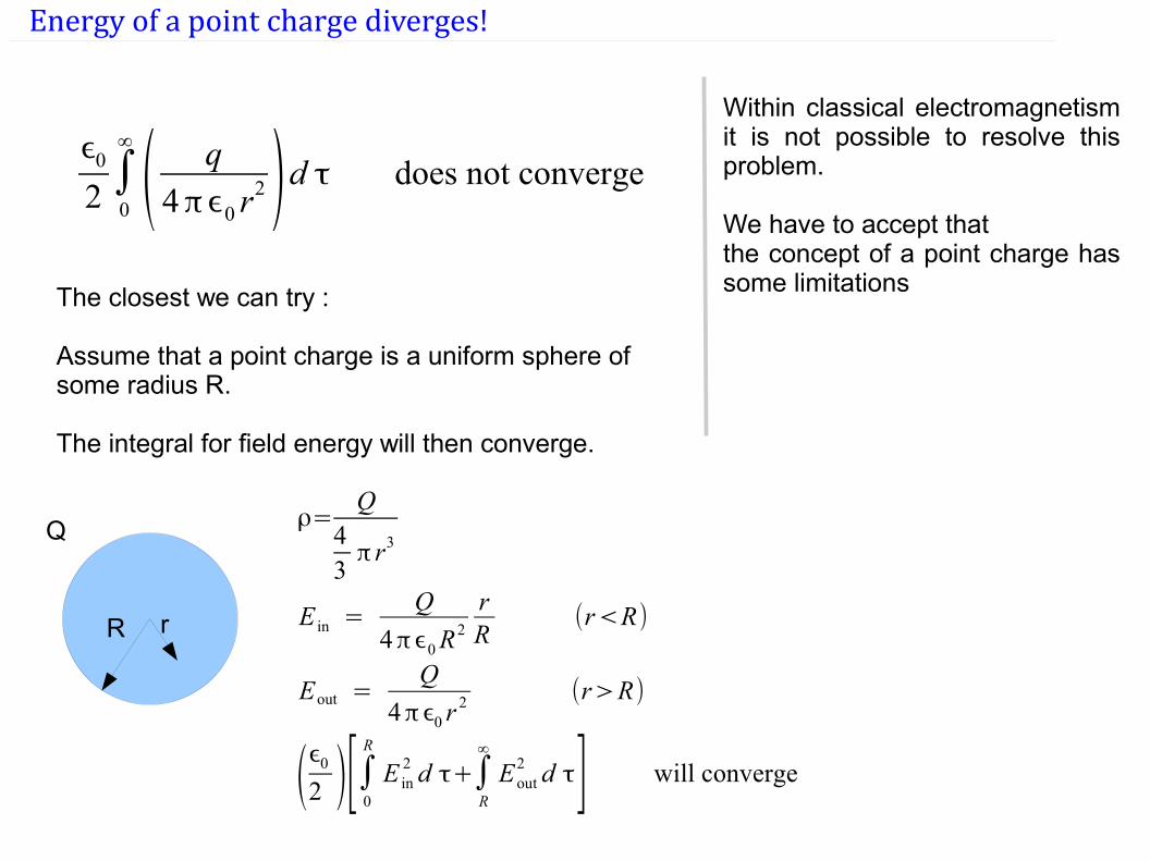
Energy of a point charge diverges!
ϵ0
2∫0
∞
( q4πϵ0 r
2)d τ does not converge
Within classical electromagnetism it is not possible to resolve this problem.
We have to accept thatthe concept of a point charge has some limitations
The closest we can try :
Assume that a point charge is a uniform sphere of some radius R.
The integral for field energy will then converge.
R
Q
r
ρ=Q
43π r3
E in =Q
4πϵ0R2
rR
(r<R)
Eout =Q
4πϵ0 r2 (r>R)
(ϵ0
2 )[∫0R
E in2 d τ+∫
R
∞
Eout2 d τ] will converge

Dielectric materials:
Field of a polarised object at a large distanceMultipole expansion of scalar potential Polar and cartesian expressions for dipole, quadrupole etcAtomic and molecular origin of the dipole momentEquivalent charge distribution Force and torque on a dipoleDefinition of the E D P vectors and boundary conditionsInterface of two dielectrics, sphere in an uniform fieldEnergy contained in Electric fields with dielectrics present
Dielectric materials
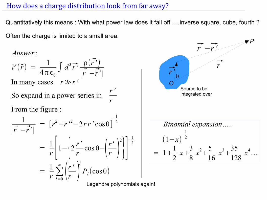
How does a charge distribution look from far away?
Quantitatively this means : With what power law does it fall off ….inverse square, cube, fourth ?
Often the charge is limited to a small area.
rr '
r −r '
Source to be integrated over
P
O
Answer :
V ( r ) =1
4πϵ0∫ d 3 r '
ρ(r ' )
| r −r ' |In many cases r≫r '
So expand in a power series inr 'r
From the figure :
1| r −r ' |
= [r2+r ' 2−2 r r ' cosθ]
−12
=1r [1−{2 r 'r cos θ−(r 'r )
2
}]−
12
=1r ∑l=0
∞
(r 'r )l
Pl (cosθ)
θ
Binomial expansion .....
(1−x)−
12
= 1+12x+
38x2+
516
x3+
35128
x4…
Legendre polynomials again!
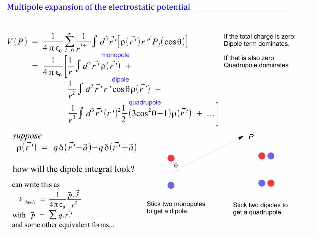
V (P ) =1
4 πϵ0∑l=0
∞ 1
r l+1∫ d3 r ' [ρ( r ' )r ' l P l(cosθ)]
=1
4 πϵ0[1r ∫d 3 r ' ρ( r ') +
1
r2∫ d3 r ' r ' cosθρ( r ') +
1
r 3∫ d3 r ' (r ' )21
2(3cos2
θ−1)ρ(r ' ) + …]
monopole
dipole
quadrupole
supposeρ( r ' ) = qδ( r '−a )−qδ(r '+a)
how will the dipole integral look?
P
θ
If the total charge is zero:Dipole term dominates.
If that is also zeroQuadrupole dominates
can write this as
V dipole =1
4πϵ0
p . r
r2
with p = ∑ qi ri 'and some other equivalent forms...
Stick two monopoles to get a dipole.
Stick two dipoles to get a quadrupole.
Multipole expansion of the electrostatic potential
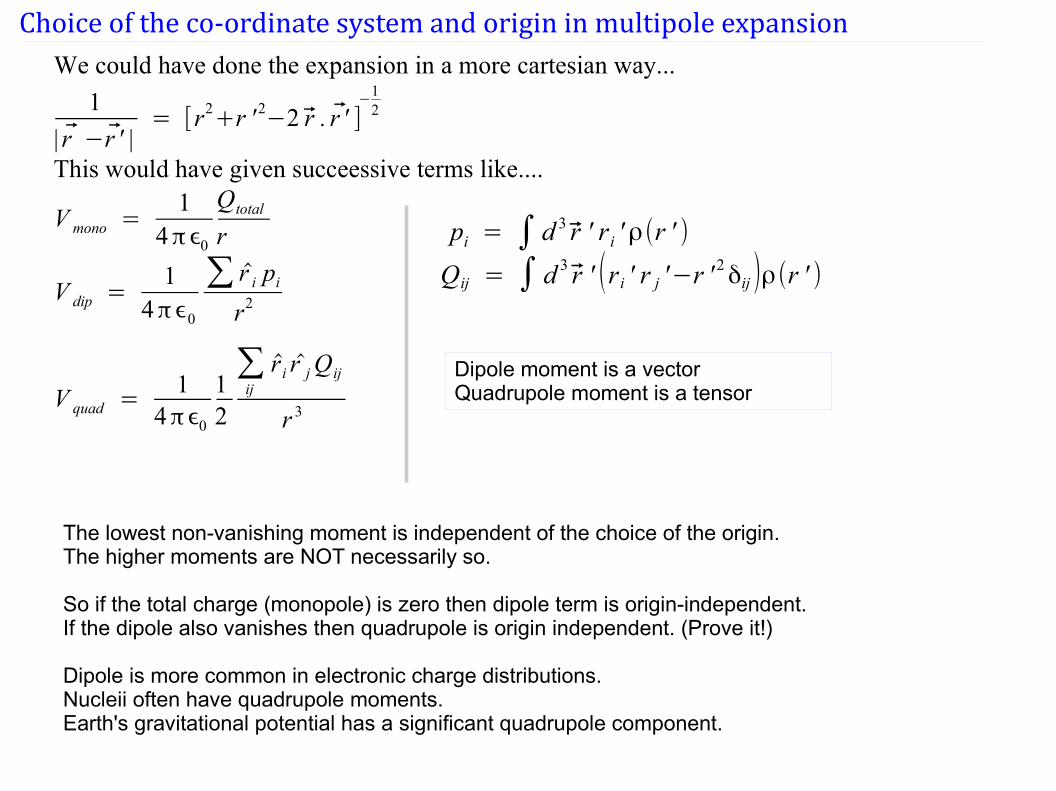
Choice of the co-ordinate system and origin in multipole expansionWe could have done the expansion in a more cartesian way...
1
| r −r ' |= [r2
+r ' 2−2 r . r ' ]−
12
This would have given succeessive terms like....
V mono =1
4πϵ0
Qtotal
r
V dip =1
4πϵ0
∑ r i pir2
V quad =1
4πϵ0
12
∑ij
r i r jQij
r 3
pi = ∫ d 3 r ' ri 'ρ(r ' )
Qij = ∫ d 3 r ' (ri ' r j '−r ' 2δij )ρ(r ' )
Dipole moment is a vectorQuadrupole moment is a tensor
The lowest non-vanishing moment is independent of the choice of the origin. The higher moments are NOT necessarily so.
So if the total charge (monopole) is zero then dipole term is origin-independent.If the dipole also vanishes then quadrupole is origin independent. (Prove it!)
Dipole is more common in electronic charge distributions.Nucleii often have quadrupole moments.Earth's gravitational potential has a significant quadrupole component.
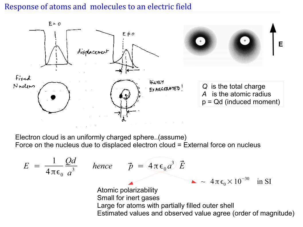
Response of atoms and molecules to an electric field
E
Electron cloud is an uniformly charged sphere..(assume) Force on the nucleus due to displaced electron cloud = External force on nucleus
E =1
4πϵ0
Qd
a3 hence p = 4πϵ0a3 E
Atomic polarizabilitySmall for inert gasesLarge for atoms with partially filled outer shellEstimated values and observed value agree (order of magnitude)
Q is the total chargeA is the atomic radiusp = Qd (induced moment)
~ 4πϵ0×10−30 in SI
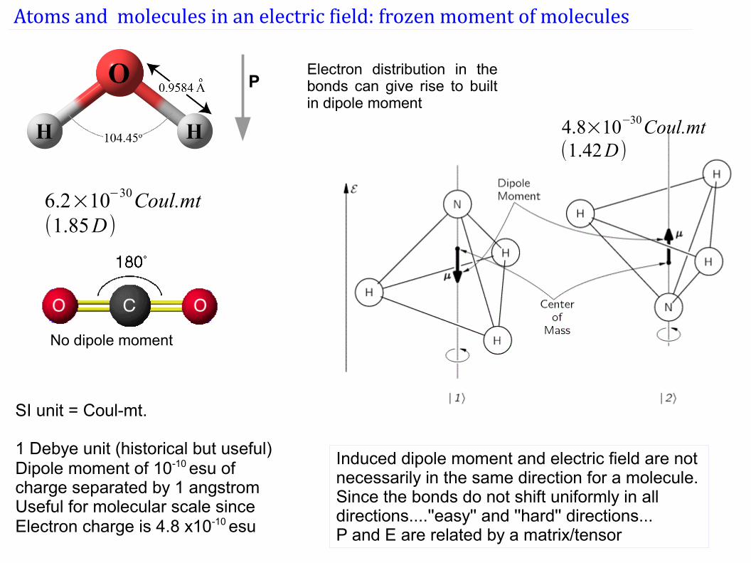
Atoms and molecules in an electric field: frozen moment of molecules
PElectron distribution in the bonds can give rise to built in dipole moment
No dipole moment
6.2×10⁻³⁰Coul.mt(1.85D)
4.8×10⁻³⁰Coul.mt(1.42D)
SI unit = Coul-mt. 1 Debye unit (historical but useful)Dipole moment of 10-10 esu of charge separated by 1 angstromUseful for molecular scale since Electron charge is 4.8 x10⁻¹⁰ esu
Induced dipole moment and electric field are not necessarily in the same direction for a molecule.Since the bonds do not shift uniformly in all directions....''easy'' and ''hard'' directions...P and E are related by a matrix/tensor
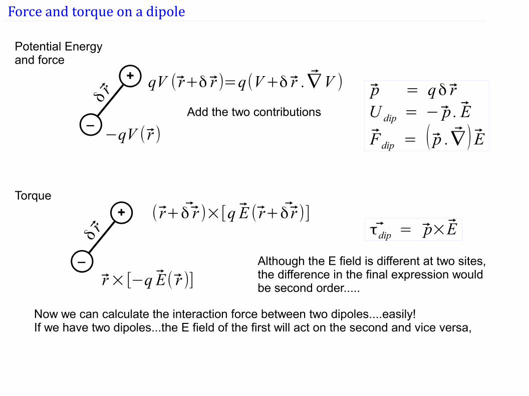
Force and torque on a dipole
_
+
−qV ( r )
qV ( r+δ r )=q(V+δ r . ∇ V )
Potential Energy and force
p = qδ rU dip = − p . E
Fdip = ( p .∇ ) EAdd the two contributions
Torque
_
+
r×[−q E( r )]
( r+δ r )×[q E ( r+δ r )]τdip = p×E
Although the E field is different at two sites, the difference in the final expression would be second order.....
Now we can calculate the interaction force between two dipoles....easily!If we have two dipoles...the E field of the first will act on the second and vice versa,
δr
δr
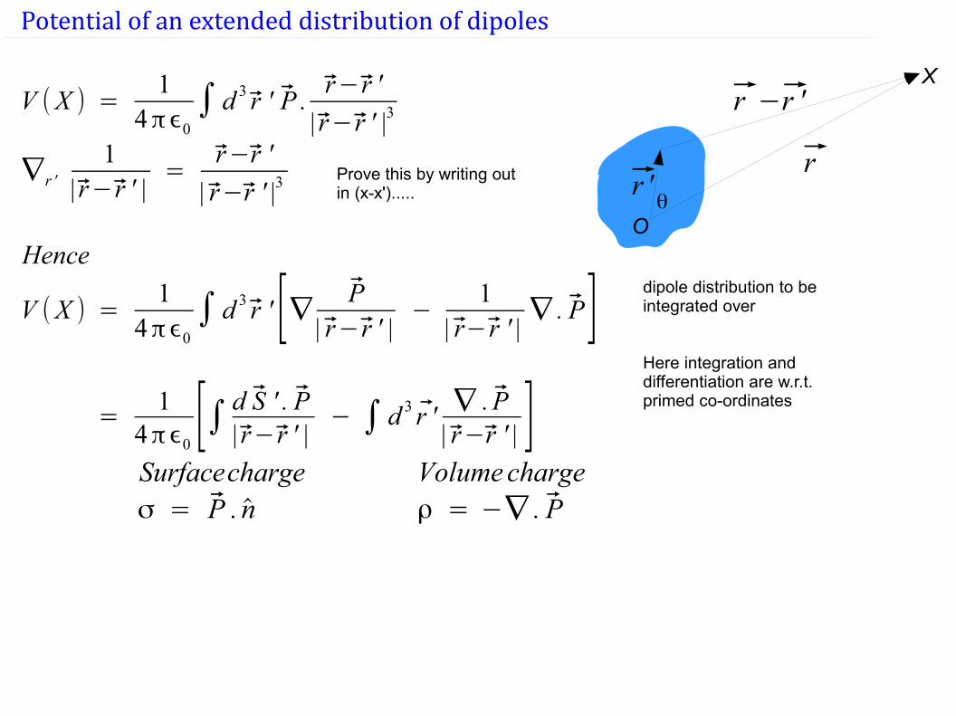
Potential of an extended distribution of dipoles
dipole distribution to be integrated over
Here integration and differentiation are w.r.t. primed co-ordinates
rr '
r −r 'X
Oθ
V (X ) =1
4πϵ0∫ d 3 r ' P .
r− r '
| r− r ' |3
∇r '
1| r− r ' |
=r−r '
| r−r ' |3
Hence
V (X ) =1
4πϵ0∫ d 3 r ' [∇ P
| r− r ' |−
1| r− r ' |
∇ . P]
=1
4πϵ0[∫ d S ' . P| r− r ' |
− ∫ d 3 r '∇ . P
| r−r ' | ]Surfacechargeσ = P . n
Volumechargeρ = −∇ . P
Prove this by writing outin (x-x').....
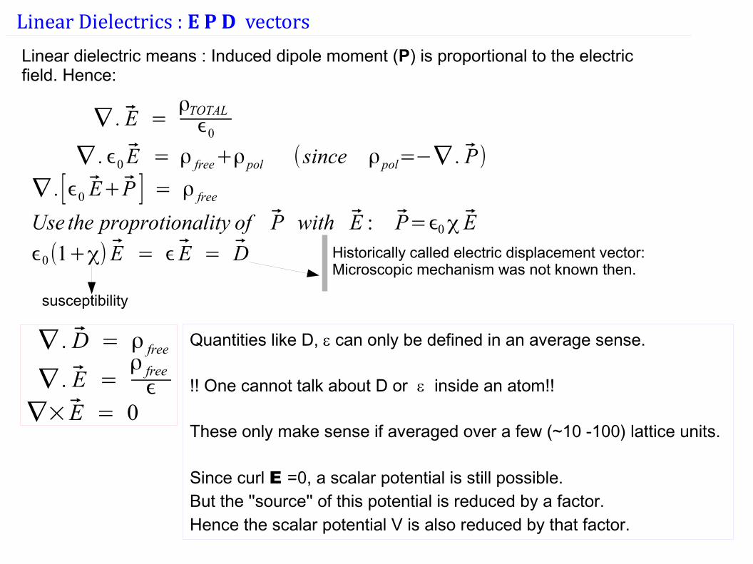
Linear Dielectrics : E P D vectors
Linear dielectric means : Induced dipole moment (P) is proportional to the electric field. Hence:
∇ . E =ρTOTALϵ0
∇ .ϵ0 E = ρ free+ρpol (since ρpol=−∇ . P)
∇ .[ϵ0 E+P ] = ρ free
Use the proprotionality of P with E : P=ϵ0χ E
ϵ0(1+χ) E = ϵ E = D
susceptibility
Historically called electric displacement vector:Microscopic mechanism was not known then.
Quantities like D, e can only be defined in an average sense. !! One cannot talk about D or e inside an atom!!
These only make sense if averaged over a few (~10 -100) lattice units.
Since curl E =0, a scalar potential is still possible. But the ''source'' of this potential is reduced by a factor. Hence the scalar potential V is also reduced by that factor.
∇ . D = ρ free
∇ . E =ρ freeϵ
∇× E = 0
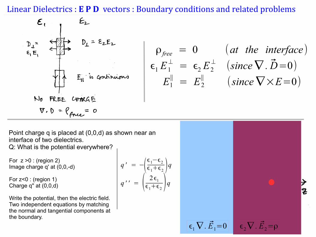
Linear Dielectrics : E P D vectors : Boundary conditions and related problems
ρ free = 0 (at the interface)
ϵ1 E1⊥= ϵ2 E2
⊥(since∇ . D=0)
E1∥= E2
∥(since∇×E=0)
Point charge q is placed at (0,0,d) as shown near an interface of two dielectrics. Q: What is the potential everywhere?
ϵ2∇ . E2=ρϵ1∇ . E1=0
For z >0 : (region 2)Image charge q' at (0,0,-d)
For z<0 : (region 1)Charge q'' at (0,0,d)
Write the potential, then the electric field.Two independent equations by matching the normal and tangential components at the boundary.
q ' = −(ϵ1−ϵ2
ϵ1+ϵ2 )qq ' ' = ( 2ϵ1
ϵ1+ϵ2 )q
Linear Dielectrics : A uniformly polarised sphere
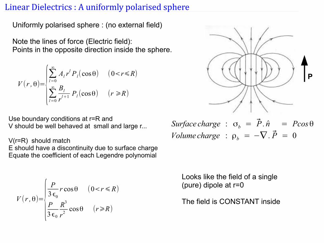
Uniformly polarised sphere : (no external field)
Note the lines of force (Electric field): Points in the opposite direction inside the sphere.
PV (r ,θ)={
∑l=0
∞
Al rl P l(cosθ) (0<r⩽R)
∑l=0
∞ Bl
r l+1 Pl (cosθ) (r ⩾R)
Use boundary conditions at r=R andV should be well behaved at small and large r...
V(r=R) should matchE should have a discontinuity due to surface chargeEquate the coefficient of each Legendre polynomial
V (r ,θ)={P
3ϵ0
r cosθ (0<r⩽R)
P3ϵ0
R3
r2cosθ (r⩾R)
Surface charge : σb = P . n = Pcosθ
Volumecharge : ρb = −∇ . P = 0
Looks like the field of a single (pure) dipole at r=0
The field is CONSTANT inside
Linear Dielectrics : A dielectric sphere in an uniform field
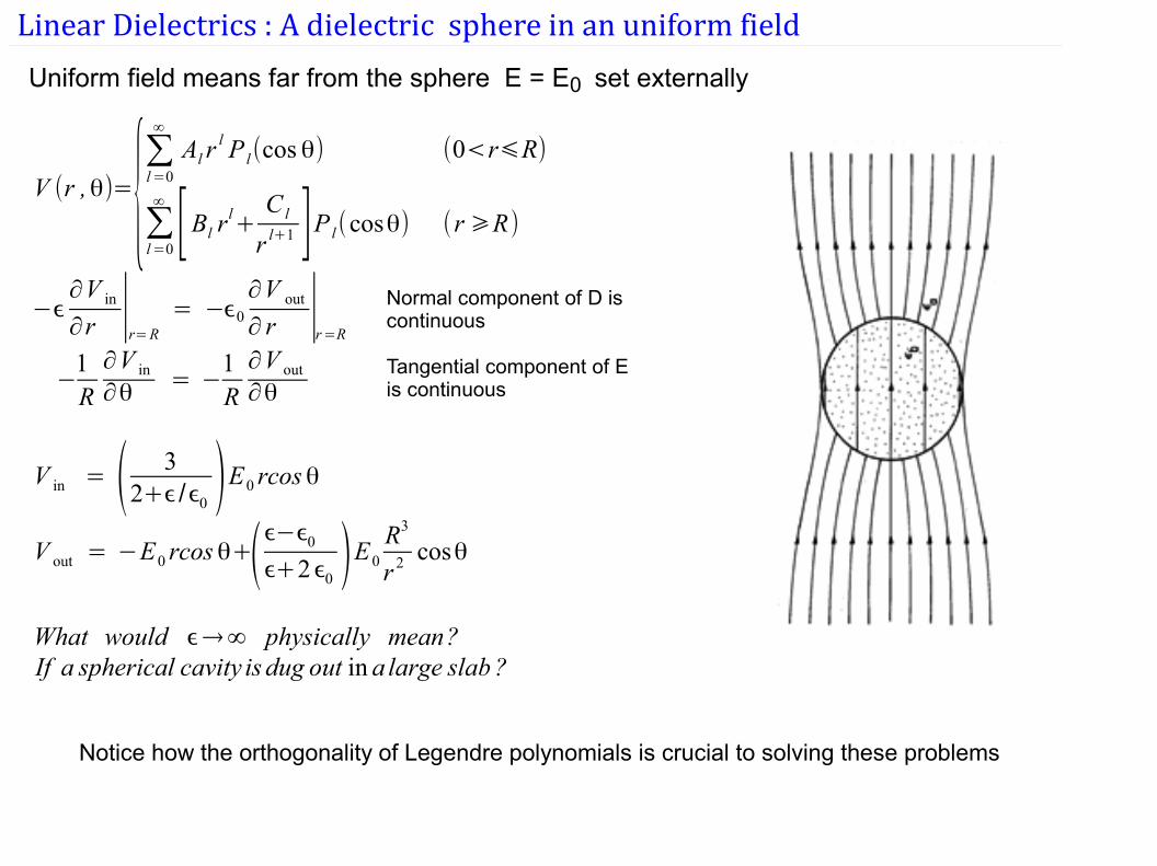
Uniform field means far from the sphere E = E0 set externally
V (r ,θ)={∑l=0
∞
Al rl P l(cos θ) (0<r⩽R)
∑l=0
∞
[Bl rl+C l
r l+1 ]P l(cosθ) (r⩾R)
−ϵ∂V in
∂r ∣r=R
= −ϵ0
∂V out
∂ r ∣r=R
−1R
∂V in
∂θ = −1R
∂V out
∂θ
V in = ( 32+ϵ/ϵ0 )E0 rcosθ
V out = −E0 rcosθ+(ϵ−ϵ0
ϵ+2ϵ0 )E0
R3
r 2 cosθ
What would ϵ→∞ physically mean?If a spherical cavity is dug out in a large slab ?
Normal component of D is continuous
Tangential component of E is continuous
Notice how the orthogonality of Legendre polynomials is crucial to solving these problems
Linear Dielectrics : A capacitor with a dielectric slab
e+sf + + + + + + + + + + + + + + +
- - - - - - - - - - - - - - - - - - - - - - -
-sb
-sf
+sb
- - - - - - - - - -
+ + + + + + + + +
+ + + + + + + + + + + + + + +
- - - - - - - - - - - - - - - - - - - - - - --sf
+sf
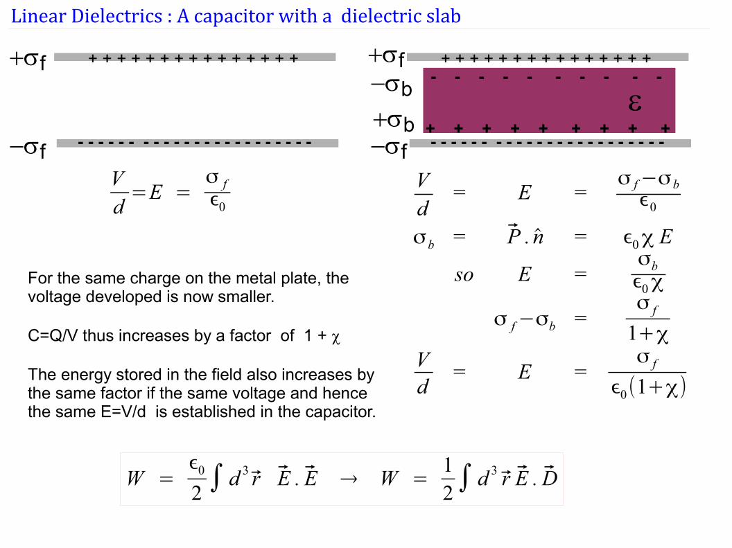
Vd=E =
σ fϵ0
Vd
= E =σ f−σbϵ0
σb = P . n = ϵ0χ E
so E =σbϵ0χ
σ f−σb =σ f
1+χVd
= E =σ f
ϵ0(1+χ)
For the same charge on the metal plate, the voltage developed is now smaller.
C=Q/V thus increases by a factor of 1 + c
The energy stored in the field also increases by the same factor if the same voltage and hence the same E=V/d is established in the capacitor.
W =ϵ0
2∫ d 3 r E . E → W =
12∫ d 3 r E . D
Magnetostatics
Magnetostatics: Field due to steady currents
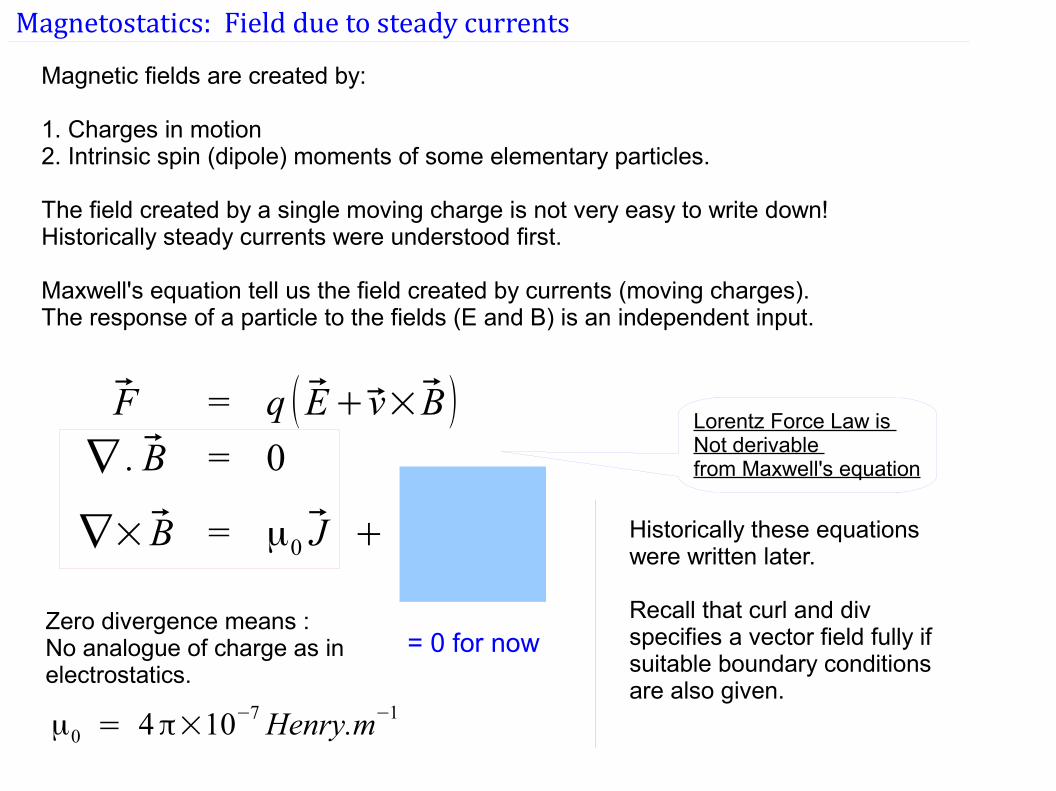
Magnetic fields are created by:
1. Charges in motion 2. Intrinsic spin (dipole) moments of some elementary particles.
The field created by a single moving charge is not very easy to write down!Historically steady currents were understood first.
Maxwell's equation tell us the field created by currents (moving charges). The response of a particle to the fields (E and B) is an independent input.
F = q ( E+ v×B)∇ . B = 0
∇× B = μ0 J + ϵ0μ0
∂ E∂ t
Lorentz Force Law is Not derivable from Maxwell's equation
Historically these equations were written later.
Recall that curl and div specifies a vector field fully if suitable boundary conditions are also given.
= 0 for nowZero divergence means :No analogue of charge as in electrostatics.
μ0 = 4π×10−7 Henry.m−1
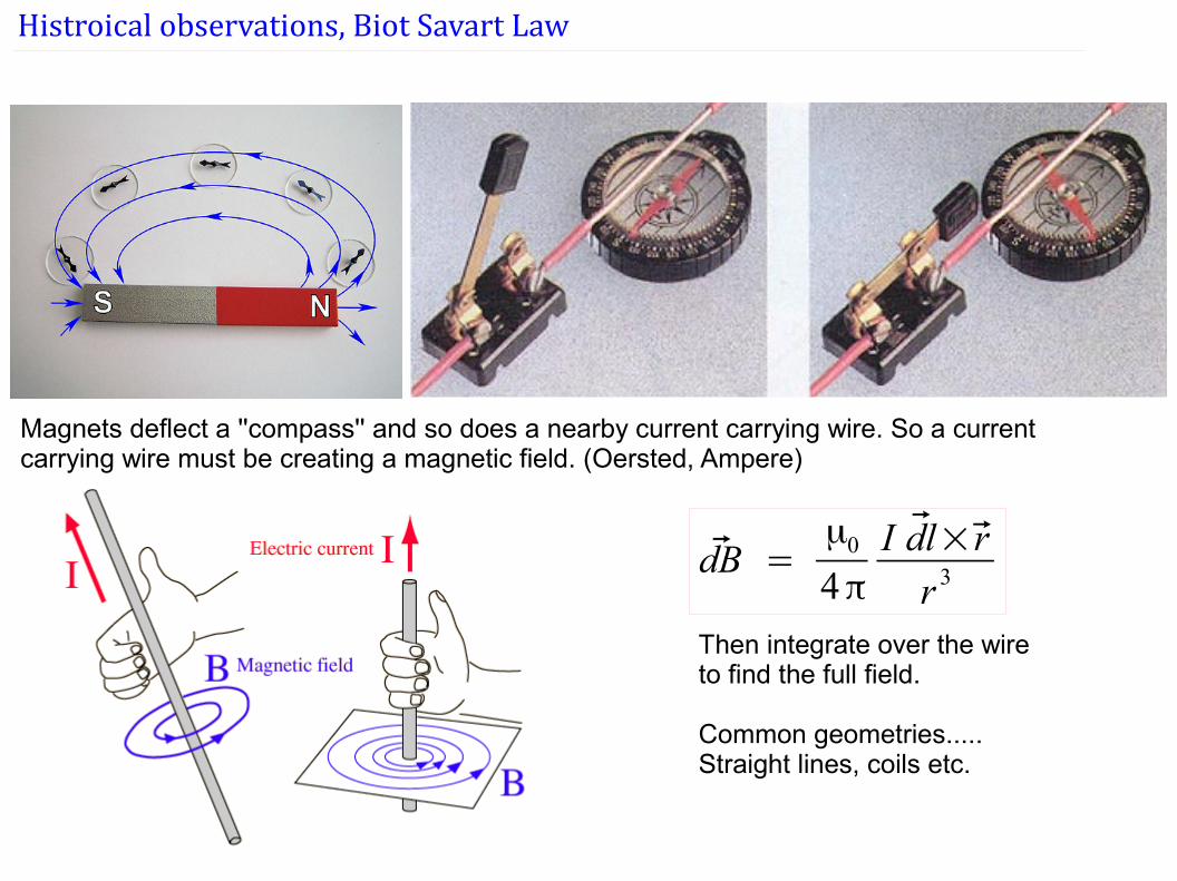
Histroical observations, Biot Savart Law
dB =μ0
4πI dl× rr 3
Magnets deflect a ''compass'' and so does a nearby current carrying wire. So a current carrying wire must be creating a magnetic field. (Oersted, Ampere)
Then integrate over the wire to find the full field.
Common geometries.....Straight lines, coils etc.
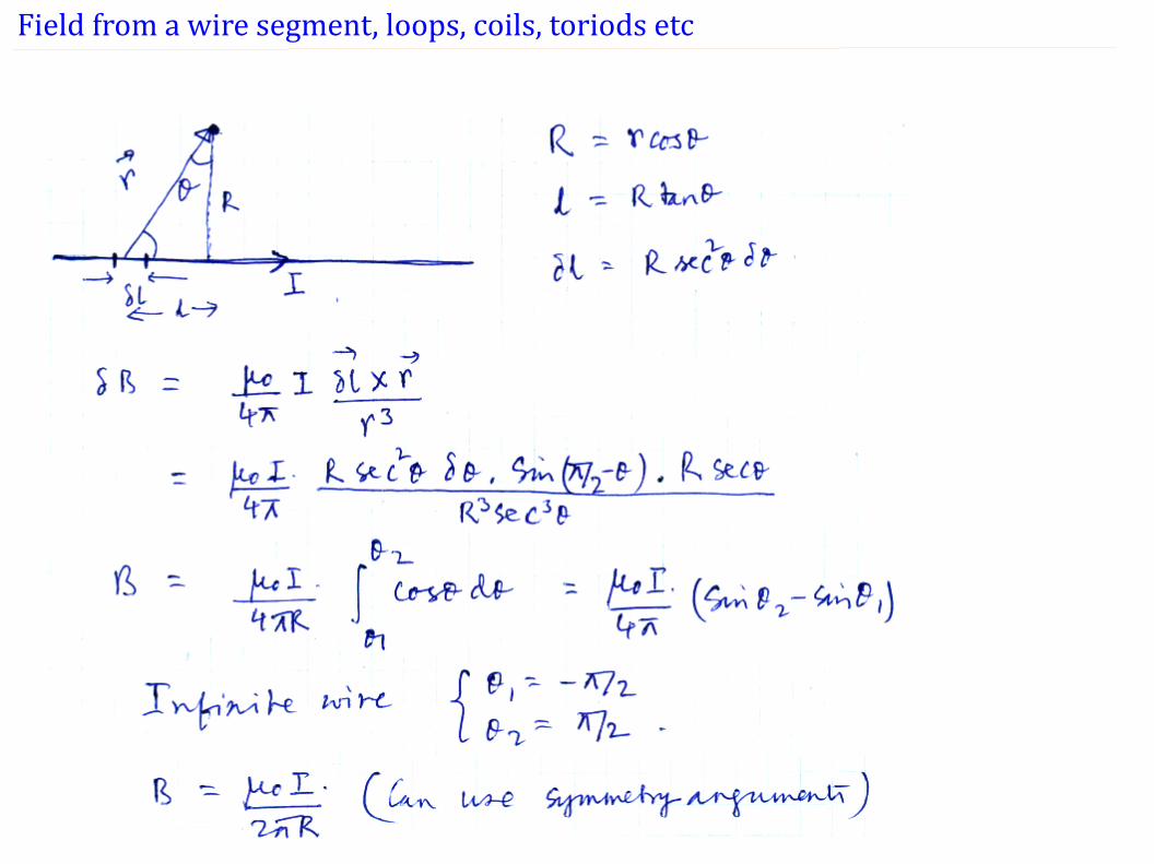
Field from a wire segment, loops, coils, toriods etc
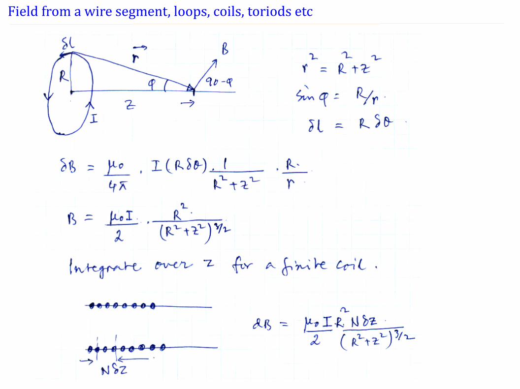
Field from a wire segment, loops, coils, toriods etc
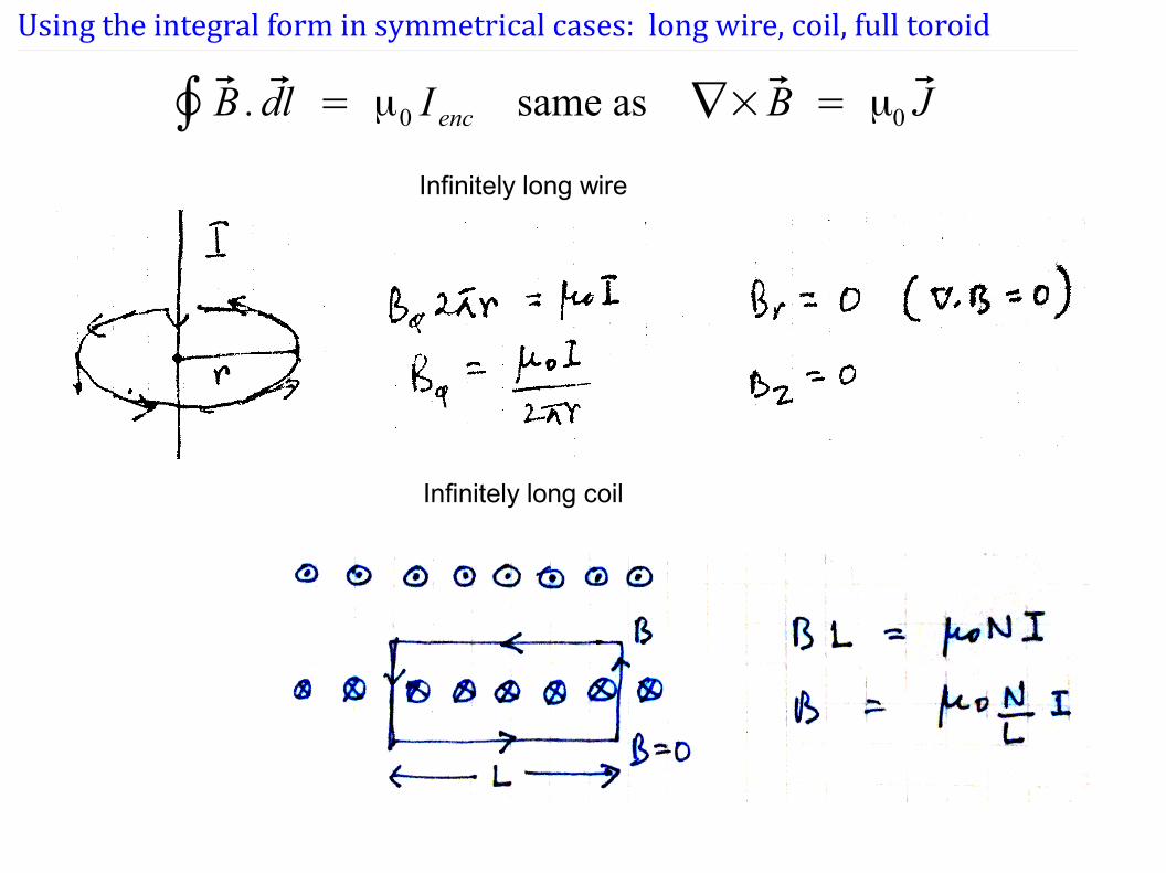
Using the integral form in symmetrical cases: long wire, coil, full toroid
∮ B . dl = μ0 I enc same as ∇× B = μ0 J
Infinitely long wire
Infinitely long coil
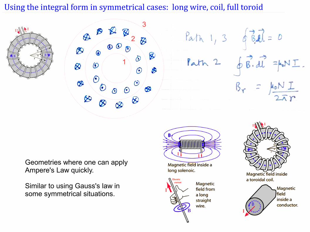
Using the integral form in symmetrical cases: long wire, coil, full toroid
1
2
3
Geometries where one can apply Ampere's Law quickly.
Similar to using Gauss's law in some symmetrical situations.
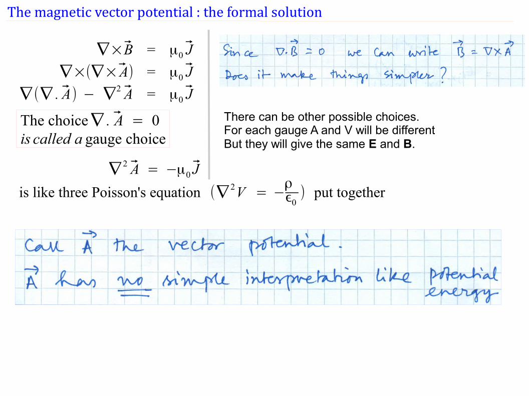
The magnetic vector potential : the formal solution
∇×B = μ0 J
∇×(∇× A) = μ0 J
∇(∇ . A) − ∇2 A = μ0 J
∇2 A = −μ0 J
is like three Poisson's equation (∇2V = −
ρϵ0) put together
The choice∇ . A = 0is called a gauge choice
There can be other possible choices.For each gauge A and V will be differentBut they will give the same E and B.
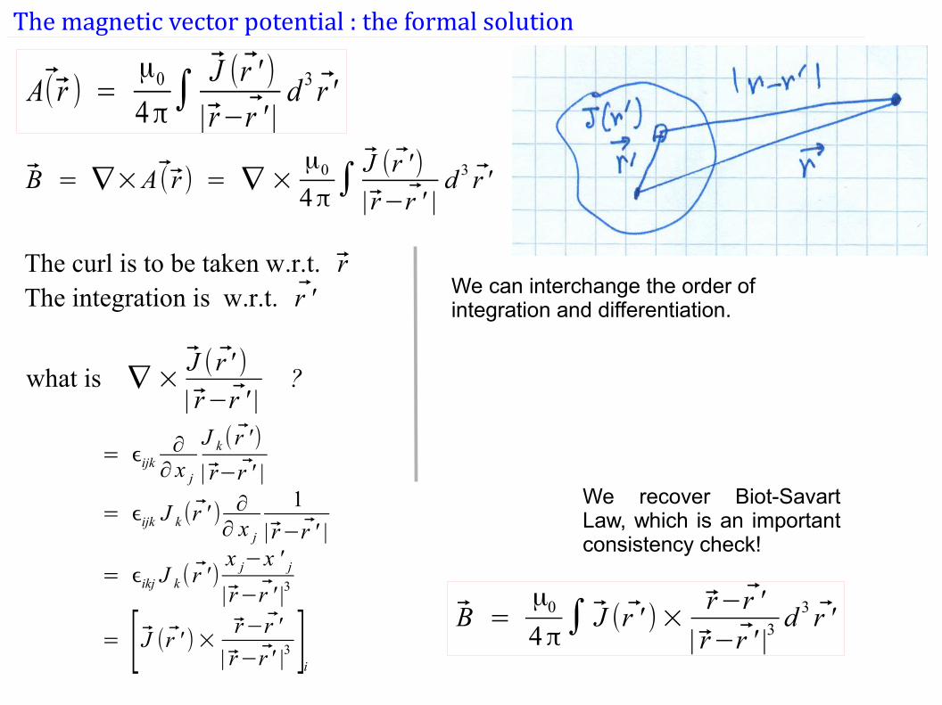
The magnetic vector potential : the formal solution
A( r ) =μ0
4π∫
J (r ' )
| r−r ' |d 3 r '
B = ∇× A( r ) = ∇ ×μ0
4π∫J (r ' )
| r−r ' |d 3 r '
The curl is to be taken w.r.t. rThe integration is w.r.t. r '
what is ∇ ×J ( r ' )
| r−r ' |?
We can interchange the order of integration and differentiation.
= ϵijk∂∂ x j
J k ( r ' )
| r−r ' |
= ϵijk J k (r ' )∂∂ x j
1
| r−r ' |
= ϵikj J k ( r ' )x j−x ' j| r−r ' |3
= [ J (r ' )× r−r '
| r−r ' |3 ]iB =
μ0
4π∫ J (r ' )×
r−r '
| r−r ' |3d 3 r '
We recover Biot-Savart Law, which is an important consistency check!
The magnetic vector potential : the choice of div A and its consequences
Our choice of A cannot affect the final result for B.
But is does effect the solution for BOTH the scalar and the vector potential.
Notice that A,V suffer from ''instantaneous change at a distance'' problem.
We do not need to care as long as it is a static/steady state solution.
But what if charge and current densities (hence A and V) are both varying arbitrarily?
The choice of A and V : how much freedom is there?
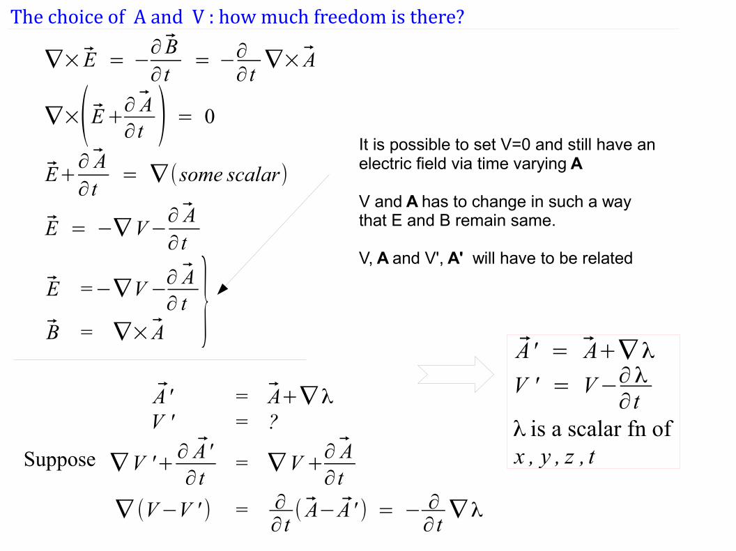
It is possible to set V=0 and still have an electric field via time varying A
V and A has to change in such a way that E and B remain same.
V, A and V', A' will have to be related
∇× E = −∂ B∂ t
= −∂∂ t
∇× A
∇×(E+∂ A∂ t ) = 0
E+∂ A∂ t
= ∇(some scalar)
E = −∇V−∂ A∂ t
E =−∇V−∂ A∂ t
B = ∇× A }
Suppose
A ' = A+∇λV ' = ?
∇V '+∂ A'∂ t
= ∇V+∂ A∂ t
∇ (V−V ' ) = ∂∂ t( A−A ' ) = − ∂
∂ t∇λ
A ' = A+∇λ
V ' = V−∂λ∂ t
λ is a scalar fn ofx , y , z , t
Multipole expansion of the magnetic vector potential
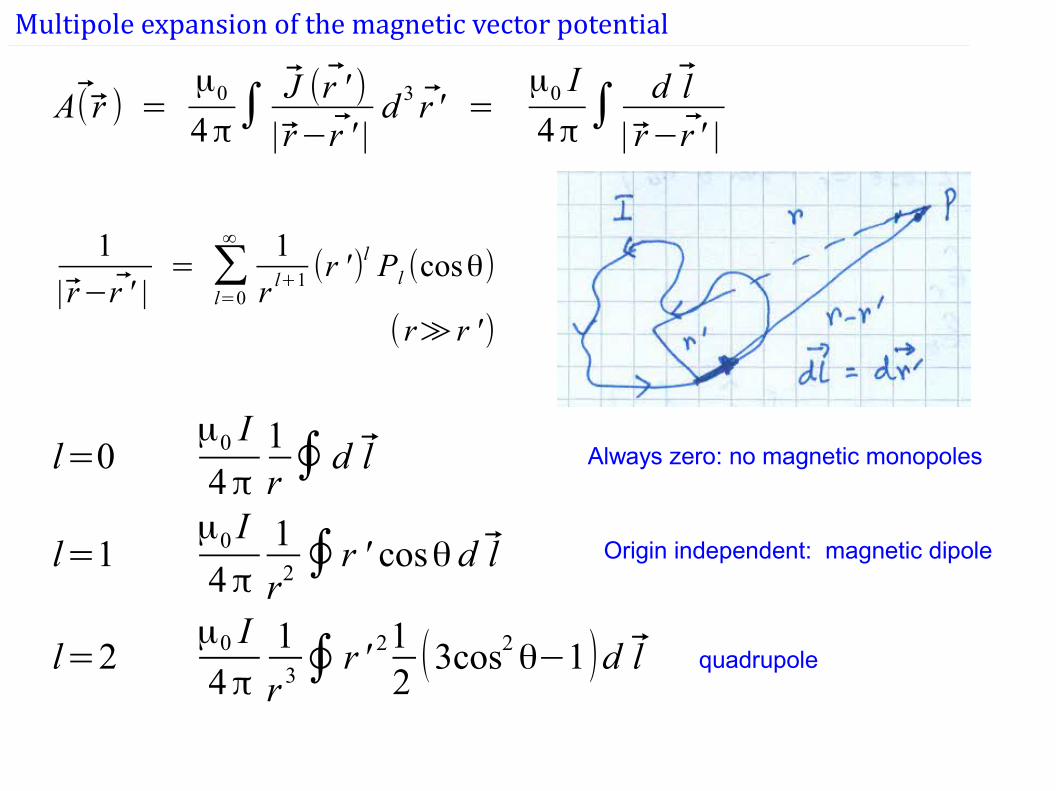
Always zero: no magnetic monopoles
Origin independent: magnetic dipole
quadrupole
A( r ) =μ0
4π∫ J (r ' )
| r−r ' |d 3 r ' =
μ0 I
4π∫ d l
| r−r ' |
1
| r−r ' |= ∑
l=0
∞ 1
r l+1 (r ')l Pl (cosθ)
(r≫r ')
l=0μ0 I
4π1r∮ d l
l=1μ0 I
4π1
r2∮r ' cosθ d l
l=2μ0 I4π
1
r 3∮ r ' 212(3cos2
θ−1)d l
Multipole expansion of the magnetic vector potential
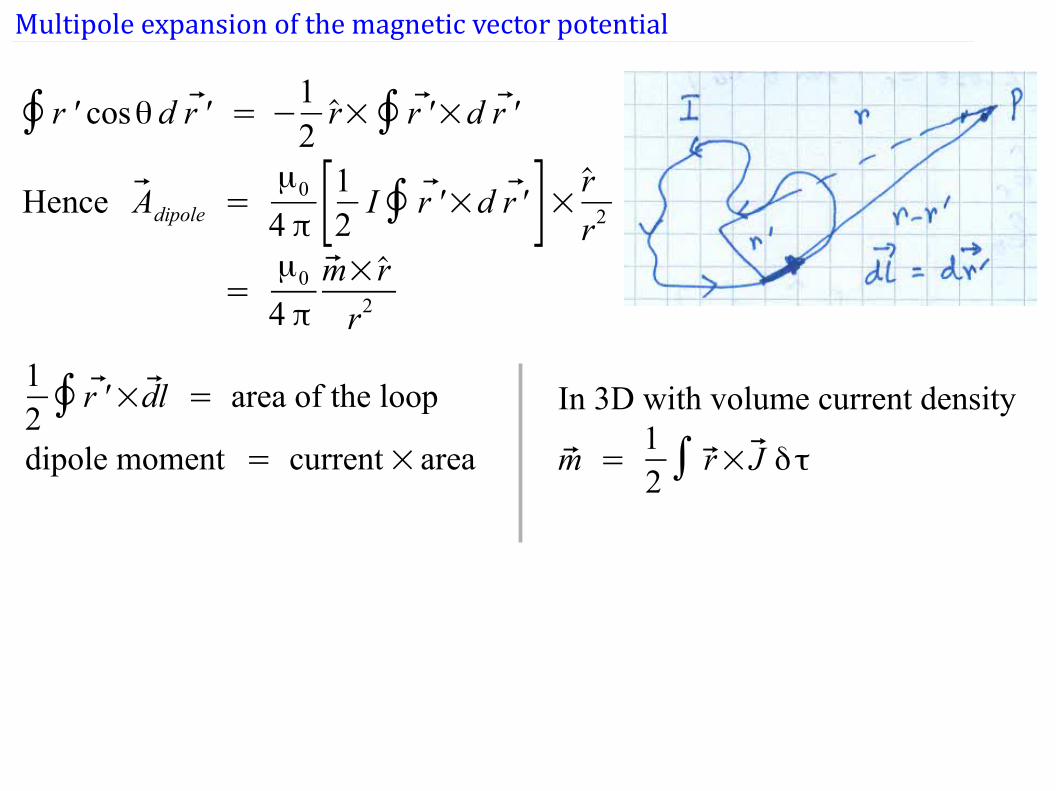
In 3D with volume current density
m =12∫ r× J δτ
12∮ r '×dl = area of the loop
dipole moment = current× area
∮r ' cosθ d r ' = −12r×∮ r '×d r '
Hence Adipole =μ0
4 π [12I∮ r '×d r ' ]× r
r2
=μ0
4 πm× r
r2
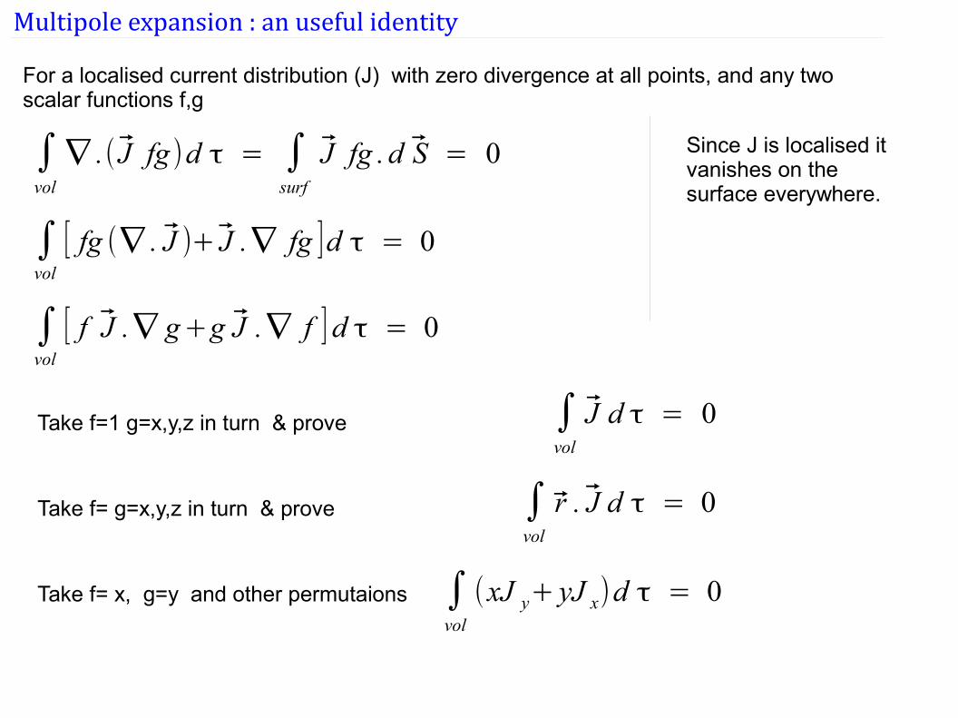
Multipole expansion : an useful identity
For a localised current distribution (J) with zero divergence at all points, and any two scalar functions f,g
∫vol
∇ .( J fg)d τ = ∫surf
J fg . d S = 0
∫vol
[ fg (∇ . J )+ J .∇ fg ]d τ = 0
∫vol
[ f J .∇ g+g J .∇ f ] d τ = 0
Since J is localised it vanishes on the surface everywhere.
Take f=1 g=x,y,z in turn & prove ∫vol
J d τ = 0
Take f= g=x,y,z in turn & prove ∫vol
r . J d τ = 0
Take f= x, g=y and other permutaions ∫vol
(xJ y+ yJ x)d τ = 0
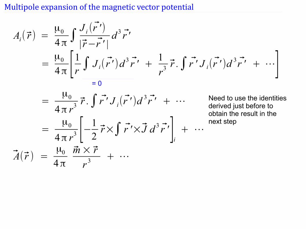
Multipole expansion of the magnetic vector potential
Ai( r ) =μ0
4π∫J i (r ' )
| r−r ' |d 3 r '
=μ0
4π [1r ∫ J i( r ' )d3 r ' +
1
r3 r .∫ r ' J i(r ' )d3 r ' + ⋯]
=μ0
4π r3 r .∫ r ' J i(r ' )d3 r ' + ⋯
=μ0
4π r3 [−12r×∫ r '× J d 3 r ']
i
+ ⋯
A( r ) =μ0
4πm× r
r 3 + ⋯
= 0
Need to use the identities derived just before to obtain the result in the next step
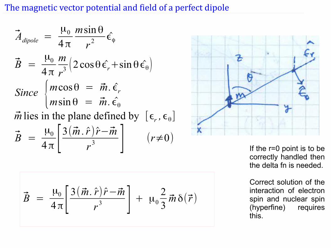
The magnetic vector potential and field of a perfect dipole
If the r=0 point is to be correctly handled then the delta fn is needed.
Correct solution of the interaction of electron spin and nuclear spin (hyperfine) requires this.
Adipole =μ0
4πmsinθ
r 2 ϵϕ
B =μ0
4πm
r3 (2cosθϵr+sinθϵθ)
Since {mcosθ = m. ϵrmsinθ = m. ϵθ
m lies in the plane defined by [ϵr ,ϵθ]
B =μ0
4π [3(m . r ) r−mr 3 ] (r≠0)
B =μ0
4π [ 3(m . r) r−m
r 3 ] + μ0
23m δ( r )
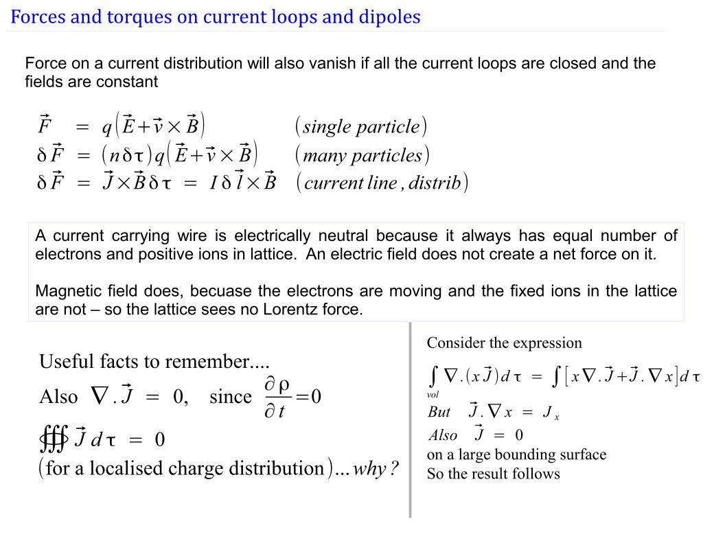
Forces and torques on current loops and dipoles
Force on a current distribution will also vanish if all the current loops are closed and the fields are constant
F = q ( E+ v× B) (single particle)
δ F = (nδτ )q( E+ v× B) (many particles)δ F = J×Bδ τ = I δ l× B (current line ,distrib)
Useful facts to remember....
Also ∇ . J = 0, since∂ρ
∂ t=0
∰ J d τ = 0(for a localised charge distribution )...why?
A current carrying wire is electrically neutral because it always has equal number of electrons and positive ions in lattice. An electric field does not create a net force on it.
Magnetic field does, becuase the electrons are moving and the fixed ions in the lattice are not – so the lattice sees no Lorentz force.
Consider the expression
∫vol
∇ .(x J )d τ = ∫ [ x∇ . J+ J .∇ x ]d τ
But J .∇ x = J x
Also J = 0on a large bounding surfaceSo the result follows
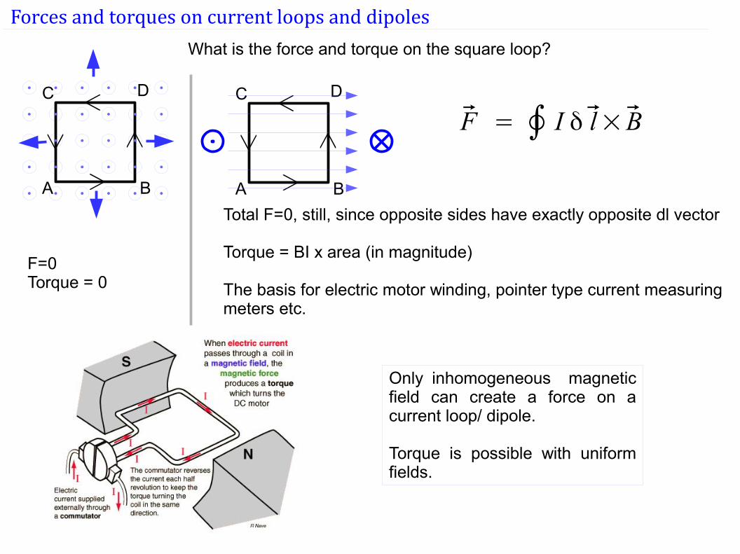
Only inhomogeneous magnetic field can create a force on a current loop/ dipole.
Torque is possible with uniform fields.
Forces and torques on current loops and dipoles
A B
C D
What is the force and torque on the square loop?
F = ∮ I δ l× B
A B
C D
Total F=0, still, since opposite sides have exactly opposite dl vector
Torque = BI x area (in magnitude)
The basis for electric motor winding, pointer type current measuring meters etc.
F=0Torque = 0
Forces and torques on current loops and dipoles
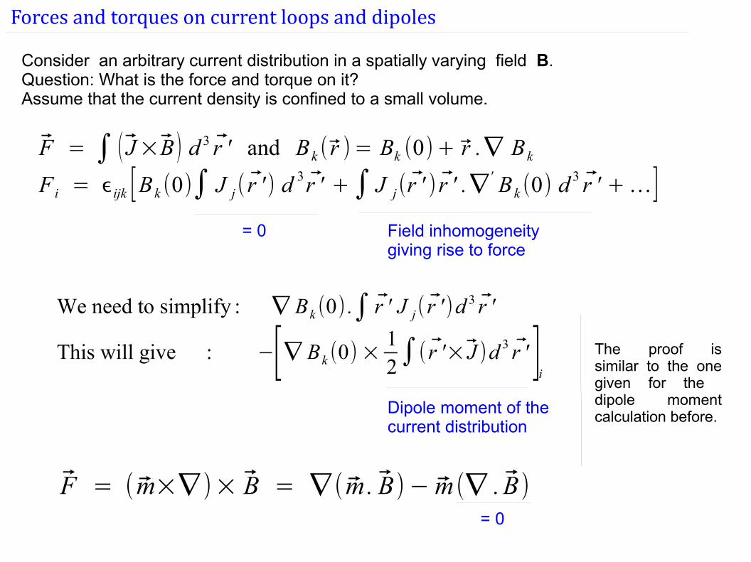
Consider an arbitrary current distribution in a spatially varying field B. Question: What is the force and torque on it?Assume that the current density is confined to a small volume.
F = ∫ ( J×B) d 3 r ' and Bk ( r )= Bk (0)+ r .∇ Bk
F i = ϵijk [Bk (0)∫ J j( r ' ) d3 r ' +∫ J j(r ' ) r ' .∇
' Bk (0) d3 r ' +…]
= 0 Field inhomogeneity giving rise to force
We need to simplify : ∇ Bk (0) .∫ r ' J j( r ')d3 r '
This will give : −[∇ Bk (0) ×12∫( r '× J )d 3 r ' ]
i
Dipole moment of the current distribution
The proof is similar to the one given for the dipole moment calculation before.
F = (m×∇)× B = ∇(m . B)− m(∇ . B)= 0
Forces and torques on current loops and dipoles
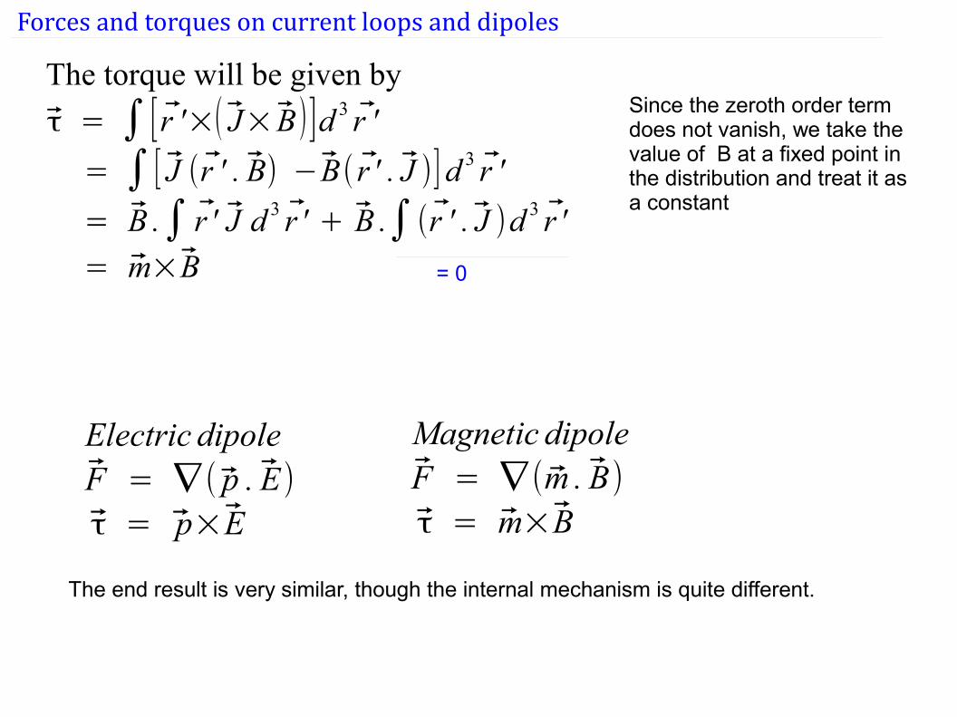
The torque will be given by
τ = ∫ [ r '×( J× B)]d 3 r '
= ∫ [ J (r ' . B) −B( r ' . J )] d 3 r '
= B .∫ r ' J d 3 r ' + B .∫(r ' . J )d 3 r '
= m×B = 0
Since the zeroth order term does not vanish, we take the value of B at a fixed point in the distribution and treat it as a constant
Electric dipoleF = ∇( p . E)τ = p×E
Magnetic dipoleF = ∇(m . B)τ = m×B
The end result is very similar, though the internal mechanism is quite different.
How does matter acquire magnetic polarisation (dipole moment)
The mechansims by which matter acquires a magnetic ''dipole moment'' per unit volume is more complex than the way electric polarisation is acquired.
A classical description of this is not really possible.
The magentic moment acquired may be
1. In the direction of the magnetic field but very weak. (paramagnetism)2. OPPOSITE to the direction of the applied field and also very weak (diamagnetism)
Para & dia magnetic effects disappear when the applied field is removed.
3. In the direction of the applied field but very strong and remains even after the initial field is removed .(ferromagnetism) This is characterised by hysteresis effects/loops/
These effects involve the dynamics of orbital electrons of an atom/ free electrons in a metal in a magnetic field, which requires a quantum mechanical description.
We will not focus on ''how'' the polarisation is acquired.
Magnetic polarisation and its description
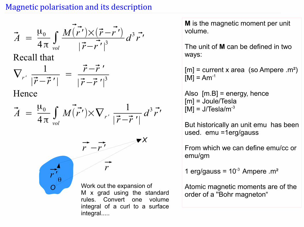
A =μ0
4π∫vol
M ( r ' )×( r−r ')
| r−r ' |3d 3 r '
Recall that
∇r '1
| r− r ' |=
r−r '
| r−r ' |3
Hence
A =μ0
4π∫vol
M ( r ' )×∇ r '
1| r−r ' |
d 3 r '
M is the magnetic moment per unit volume.
The unit of M can be defined in two ways:
[m] = current x area (so Ampere .m²) [M] = Am-1
Also [m.B] = energy, hence[m] = Joule/Tesla[M] = J/Tesla/m-3
But historically an unit emu has been used. emu =1erg/gauss
From which we can define emu/cc or emu/gm
1 erg/gauss = 10-3 Ampere .m²
Atomic magnetic moments are of the order of a ''Bohr magneton“
rr '
r −r 'X
Oθ
Work out the expansion of M x grad using the standard rules. Convert one volume integral of a curl to a surface integral.....
Magnetic polarisation and its description
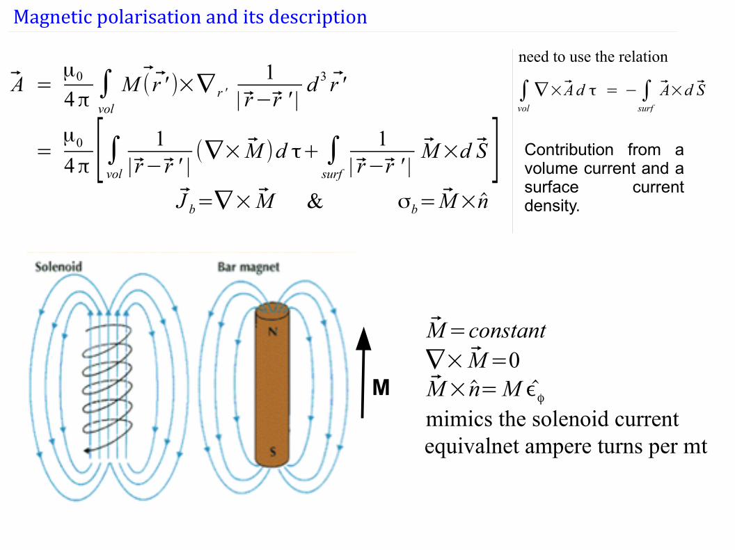
A =μ0
4π∫vol
M ( r ' )×∇ r '1
| r−r ' |d 3 r '
=μ0
4π [∫vol 1| r− r ' |
(∇× M )d τ+∫surf
1| r−r ' |
M×d S ]J b=∇× M & σb=M×n
Contribution from a volume current and a surface current density.
M=constant∇× M=0M× n=M ϵϕmimics the solenoid currentequivalnet ampere turns per mt
M
need to use the relation
∫vol
∇×A d τ = −∫surf
A×d S
Magnetic polarisation and its description: B H M vectors
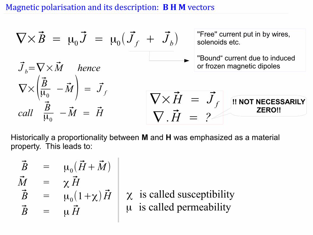
∇× B = μ0 J = μ0( J f + J b)''Free'' current put in by wires, solenoids etc.
''Bound“ current due to induced or frozen magnetic dipolesJ b=∇×M hence
∇×(Bμ0−M ) = J f
callBμ0
−M = H∇× H = J f
∇ . H = ?!! NOT NECESSARILY
ZERO!!
Historically a proportionality between M and H was emphasized as a material property. This leads to:
B = μ0(H+ M )
M = χ HB = μ0(1+χ) H
B = μ H
χ is called susceptibilityμ is called permeability
Magnetic polarisation and its description: B H M vectors : Boundary conditions
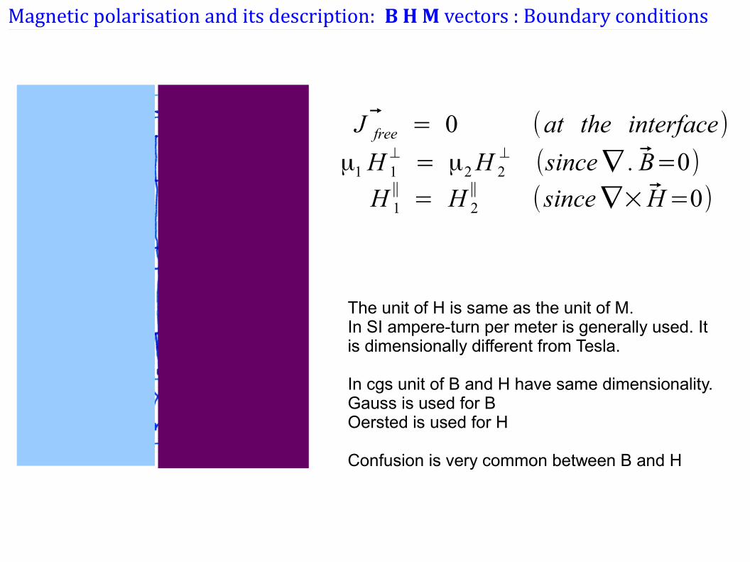
J free = 0 (at the interface)
μ1 H 1⊥= μ2H 2
⊥(since∇ . B=0)
H 1∥= H 2
∥(since∇× H=0)
The unit of H is same as the unit of M.In SI ampere-turn per meter is generally used. It is dimensionally different from Tesla.
In cgs unit of B and H have same dimensionality.Gauss is used for B Oersted is used for H
Confusion is very common between B and H
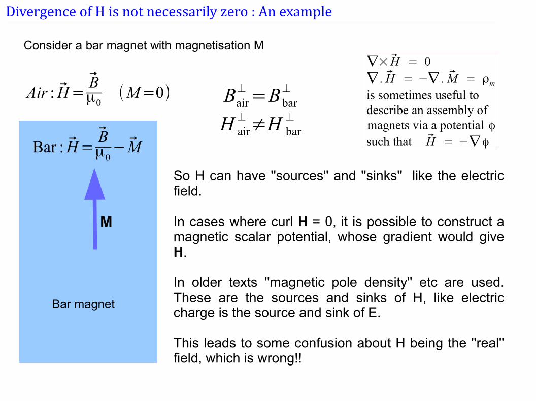
Divergence of H is not necessarily zero : An example
Consider a bar magnet with magnetisation M
M
Air : H=Bμ0
(M=0)
Bar : H=Bμ0−M
Bair⊥=Bbar
⊥
H air⊥≠H bar
⊥
So H can have ''sources'' and ''sinks'' like the electric field.
In cases where curl H = 0, it is possible to construct a magnetic scalar potential, whose gradient would give H.
In older texts ''magnetic pole density'' etc are used. These are the sources and sinks of H, like electric charge is the source and sink of E.
This leads to some confusion about H being the ''real'' field, which is wrong!!
Bar magnet
∇× H = 0∇ . H = −∇ . M = ρmis sometimes useful todescribe an assembly of magnets via a potential ϕsuch that H = −∇ϕ
Physical interpretation of the bound currents
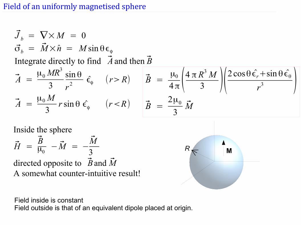
Field of an uniformly magnetised sphere
J b = ∇×M = 0
σb = M× n = M sinθϵϕIntegrate directly to find A and then B
A =μ0 MR
3
3sinθ
r 2ϵϕ (r>R)
A =μ0 M
3r sinθ ϵϕ (r<R)
B =μ0
4π(4 π R3 M
3 )(2 cosθϵr+sinθϵθr3 )
B =2μ0
3M
Inside the sphere
H =Bμ0
−M = −M3
directed opposite to B and MA somewhat counter-intuitive result!
MR
Field inside is constantField outside is that of an equivalent dipole placed at origin.
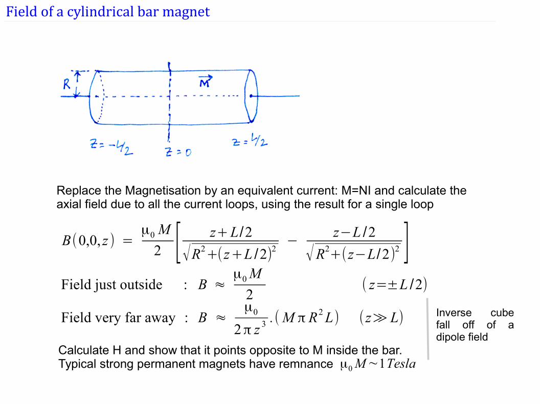
Field of a cylindrical bar magnet
Replace the Magnetisation by an equivalent current: M=NI and calculate the axial field due to all the current loops, using the result for a single loop
B(0,0, z ) =μ0 M
2 [ z+L/2
√R2+(z+L /2)2
−z−L /2
√R2+(z−L/2)2 ]
Field just outside : B ≈μ0M
2( z=±L /2)
Field very far away : B ≈μ0
2π z 3 .(M π R2L) (z≫L)
Calculate H and show that it points opposite to M inside the bar.Typical strong permanent magnets have remnance μ0M∼1Tesla
Inverse cube fall off of a dipole field
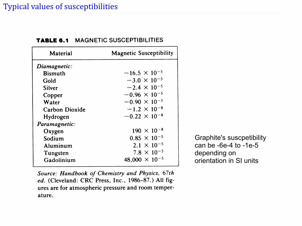
Typical values of susceptibilities
Graphite's suscpetibility can be -6e-4 to -1e-5 depending on orientation in SI units
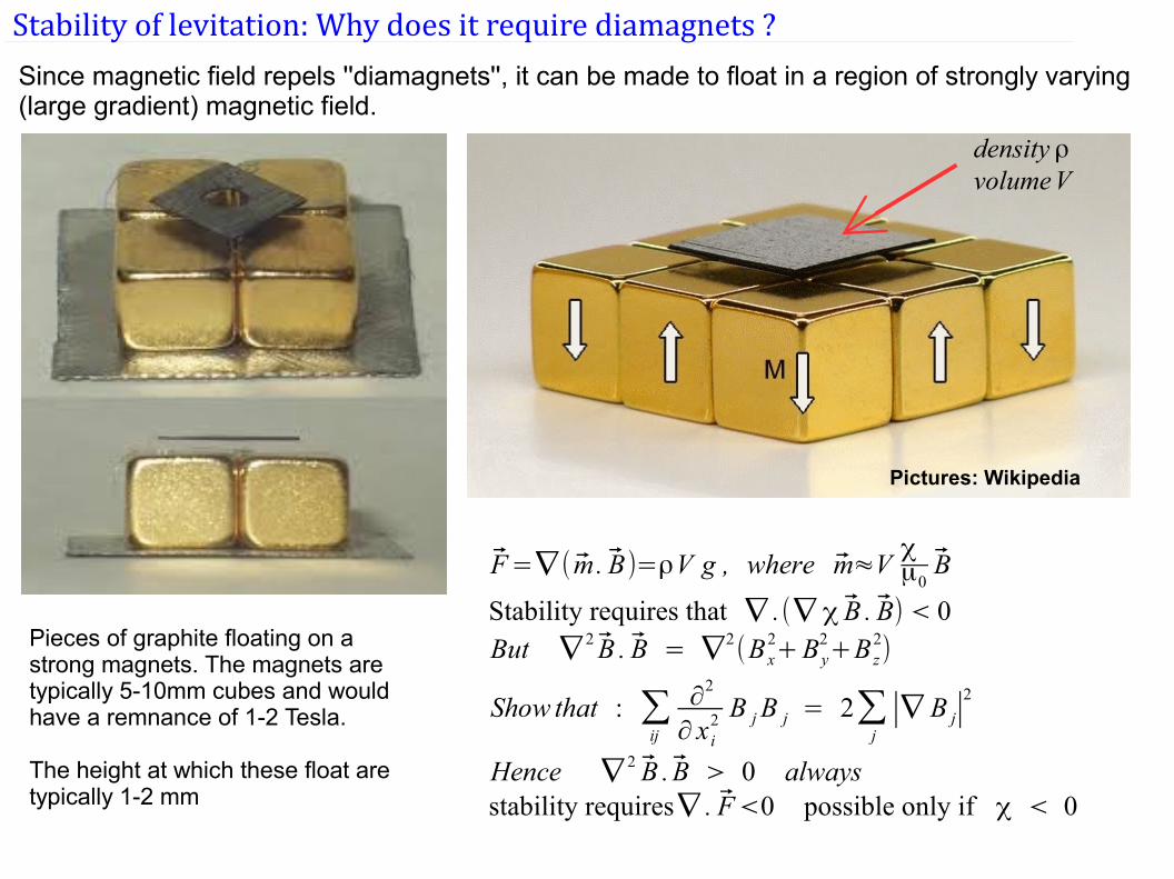
Stability of levitation: Why does it require diamagnets ?
Pieces of graphite floating on a strong magnets. The magnets are typically 5-10mm cubes and would have a remnance of 1-2 Tesla.
The height at which these float are typically 1-2 mm
Since magnetic field repels ''diamagnets'', it can be made to float in a region of strongly varying (large gradient) magnetic field.
Pictures: Wikipedia
F=∇(m. B)=ρV g , where m≈Vχμ0B
Stability requires that ∇ .(∇ χ B . B) < 0But ∇ 2 B . B = ∇2(Bx
2+By2+B z
2)
Show that : ∑ij
∂2
∂ x i2 B jB j = 2∑
j∣∇ B j∣
2
Hence ∇ 2 B . B > 0 alwaysstability requires∇ . F<0 possible only if χ < 0
density ρvolumeV
Electrodynamics
Something needs to be added to Ampere's Law. Why?Can we decouple E and B?Emergence of an wave equation. Why is f(x-vt) a ''wave''?How does the displacement current term compare with normal current?
Induced emfs: Inductors and generators
Lorentz force Law in potential form (convective derivative)Energy and momentum of the EM field.
Maxwell's equation in matterRefractive indexReflection and transmission of em waves at an interface
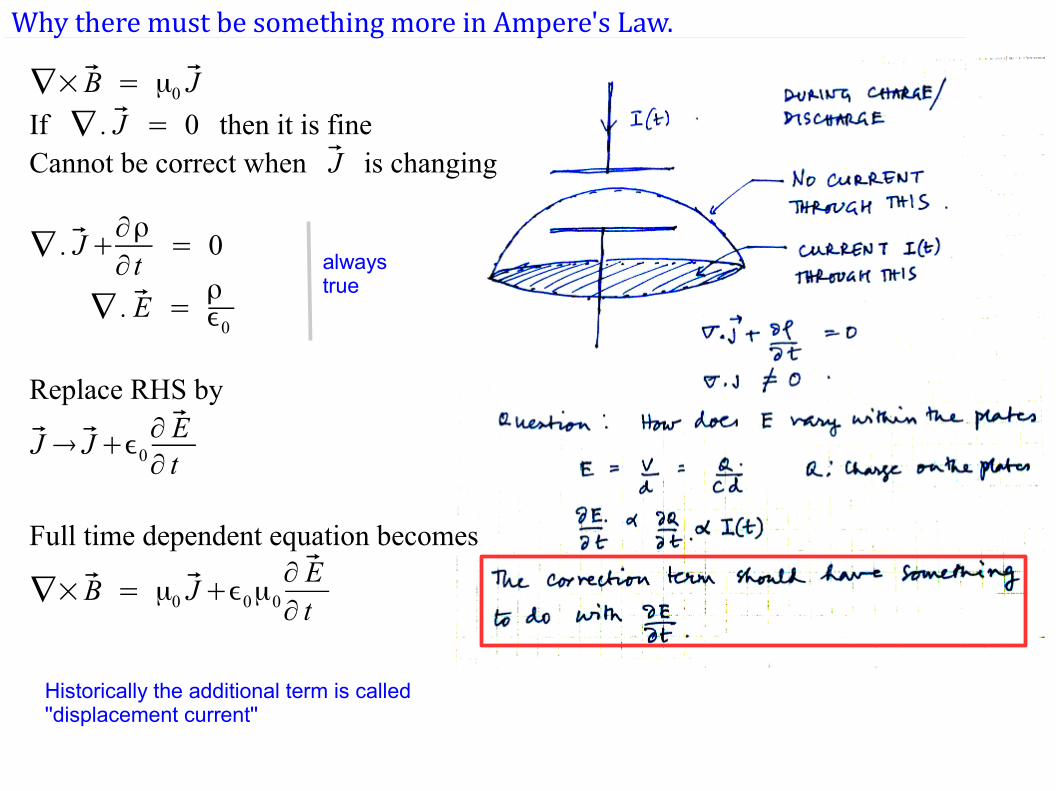
Why there must be something more in Ampere's Law.
∇× B = μ0 J
If ∇ . J = 0 then it is fineCannot be correct when J is changing
∇ . J+∂ρ
∂ t= 0
∇ . E =ρϵ0
Replace RHS by
J → J+ϵ0∂ E∂ t
Full time dependent equation becomes
∇× B = μ0 J+ϵ0μ0
∂ E∂ t
always true
Historically the additional term is called ''displacement current''
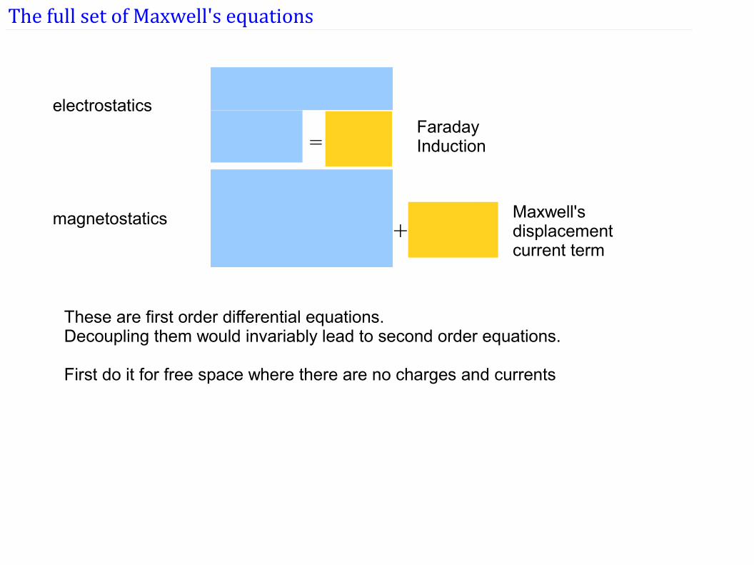
The full set of Maxwell's equations
∇ . E =ρϵ0
∇× E = −∂ B∂ t
∇ . B = 0
∇×B = μ0 J+ϵ0μ0
∂ E∂ t
electrostatics
magnetostatics
These are first order differential equations.Decoupling them would invariably lead to second order equations.
First do it for free space where there are no charges and currents
Faraday Induction
Maxwell's displacement current term
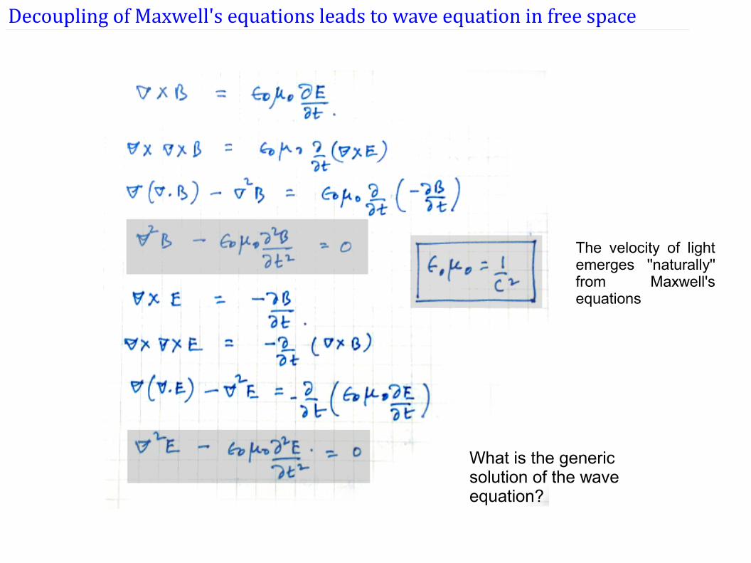
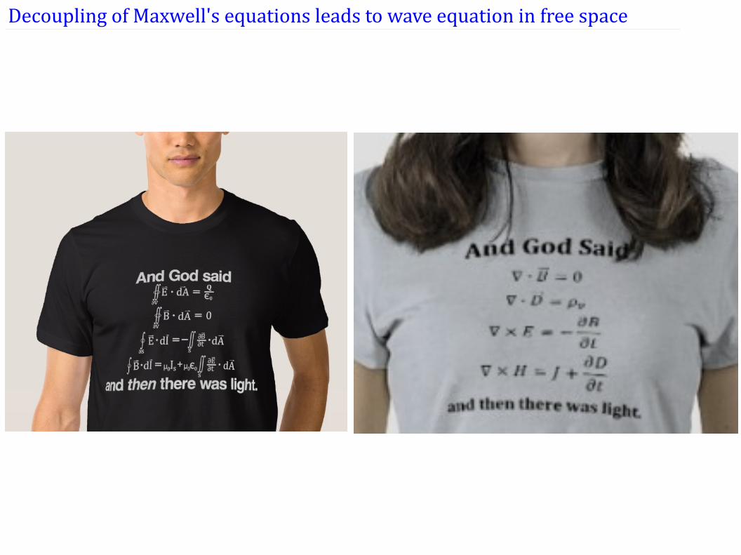
Decoupling of Maxwell's equations leads to wave equation in free space
What is the generic solution of the wave equation?
The velocity of light emerges ''naturally'' from Maxwell's equations
Decoupling of Maxwell's equations leads to wave equation in free space
When does the displacement current term become more dominant?
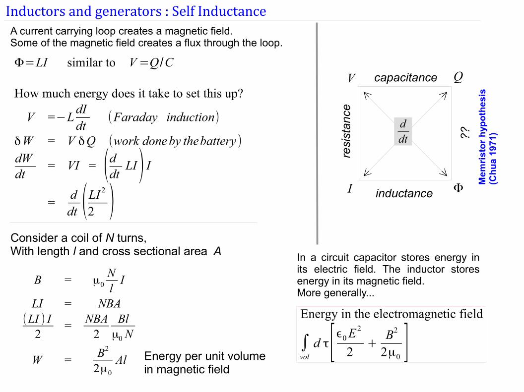
Inductors and generators : Self Inductance A current carrying loop creates a magnetic field. Some of the magnetic field creates a flux through the loop.
Φ=LI similar to V=Q /C
How much energy does it take to set this up?
V =−LdIdt
(Faraday induction)
δW = V δQ (work doneby thebattery )dWdt
= VI = (ddt LI) I=
ddt (LI
2
2 )
ddt
V Q
I Φ
capacitance
resi
stan
ce
inductance
??M
emri
sto
r h
ypo
thes
is(C
hu
a 19
71)
Consider a coil of N turns, With length l and cross sectional area A
B = μ0NlI
LI = NBA(LI ) I
2=
NBA2
Blμ0 N
W =B2
2μ0
Al Energy per unit volume in magnetic field
Energy in the electromagnetic field
∫vol
d τ[ϵ0E2
2+
B2
2μ0]
In a circuit capacitor stores energy in its electric field. The inductor stores energy in its magnetic field.More generally...
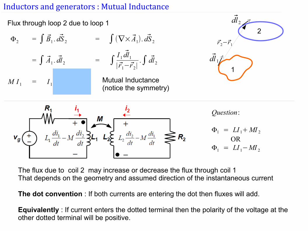
Inductors and generators : Mutual Inductance
1
2
dl 2
dl 1
r 2−r1
Flux through loop 2 due to loop 1
Φ2 = ∫ B1 . dS 2 = ∫(∇× A1) . dS 2
= ∫ A1 . dl 2 = ∫I 1 dl1| r1−r 2 |
.∫ dl 2
M I 1 = I 1∮∮dl1 . dl 2
| r1−r2 |Mutual Inductance(notice the symmetry)
Question :
Φ1 = LI 1+MI 2
ORΦ1 = LI 1−MI 2
The flux due to coil 2 may increase or decrease the flux through coil 1That depends on the geometry and assumed direction of the instantaneous current
The dot convention : If both currents are entering the dot then fluxes will add.
Equivalently : If current enters the dotted terminal then the polarity of the voltage at the other dotted terminal will be positive.
Inductors and generators : Mutual Inductance : Energy stored in the full system
How much is the energy stored in the system L1 + L2 ?
W=L1 I 12+L2 I 2
2+ MI 1 I 2 When all currents either enter or leave the dot
W=L1 I 12+L2 I 2
2− MI 1 I 2 When one current enters and the other leaves the dot
This follows from the relation between dot and the addition/subtraction of fluxCan be generalised to an arbitrary number of coupled linear inductors
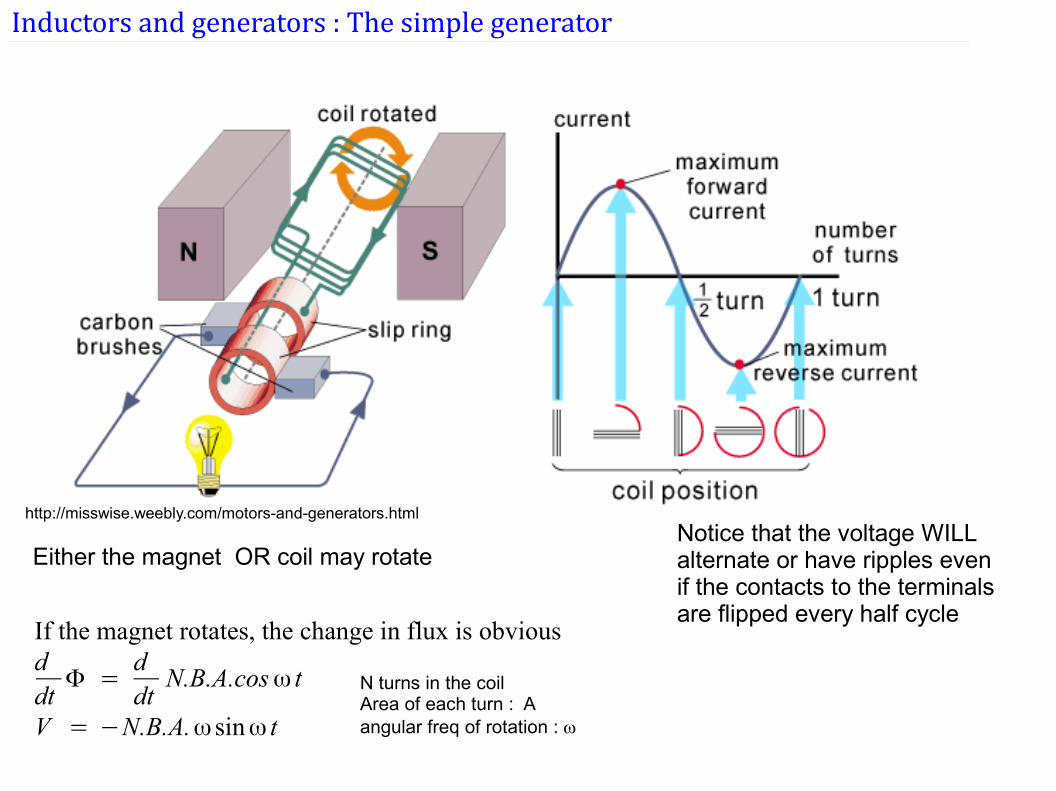
Inductors and generators : The simple generator
http://misswise.weebly.com/motors-and-generators.html
If the magnet rotates, the change in flux is obviousddtΦ =
ddt
N.B.A.cosω t
V = −N.B.A.ω sinω t
N turns in the coilArea of each turn : Aangular freq of rotation : w
Notice that the voltage WILL alternate or have ripples even if the contacts to the terminals are flipped every half cycle
Either the magnet OR coil may rotate
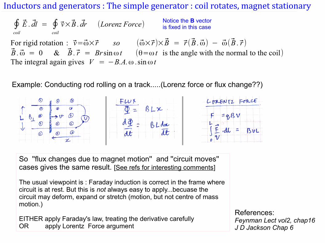
Inductors and generators : The simple generator : coil rotates, magnet stationary
∮coil
E . dl = ∮coil
v×B . dr (Lorenz Force) Notice the B vector is fixed in this case
For rigid rotation : v=ω× r so (ω× r )×B = r ( B . ω) − ω( B . r )B . ω = 0 & B . r = Br sinω t (θ=ω t is the angle with the normal to the coil)The integral again gives V = −B.A.ω .sinω t
So ''flux changes due to magnet motion'' and ''circuit moves'' cases gives the same result. [See refs for interesting comments]
The usual viewpoint is : Faraday induction is correct in the frame where circuit is at rest. But this is not always easy to apply...becuase the circuit may deform, expand or stretch (motion, but not centre of mass motion.)
EITHER apply Faraday's law, treating the derivative carefully OR apply Lorentz Force argument
References:Feynman Lect vol2, chap16J D Jackson Chap 6
Example: Conducting rod rolling on a track.....(Lorenz force or flux change??)
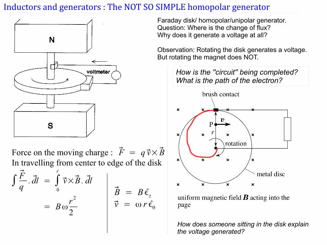
Inductors and generators : The NOT SO SIMPLE homopolar generatorFaraday disk/ homopolar/unipolar generator.Question: Where is the change of flux? Why does it generate a voltage at all?
Observation: Rotating the disk generates a voltage.But rotating the magnet does NOT.
How is the ''circuit'' being completed?What is the path of the electron?
Force on the moving charge : F = q v× BIn travelling from center to edge of the disk
∫ Fq. dl = ∫
0
r
v×B . dl
= Bωr 2
2
B = B ϵzv = ω r ϵθ
How does someone sitting in the disk explain the voltage generated?
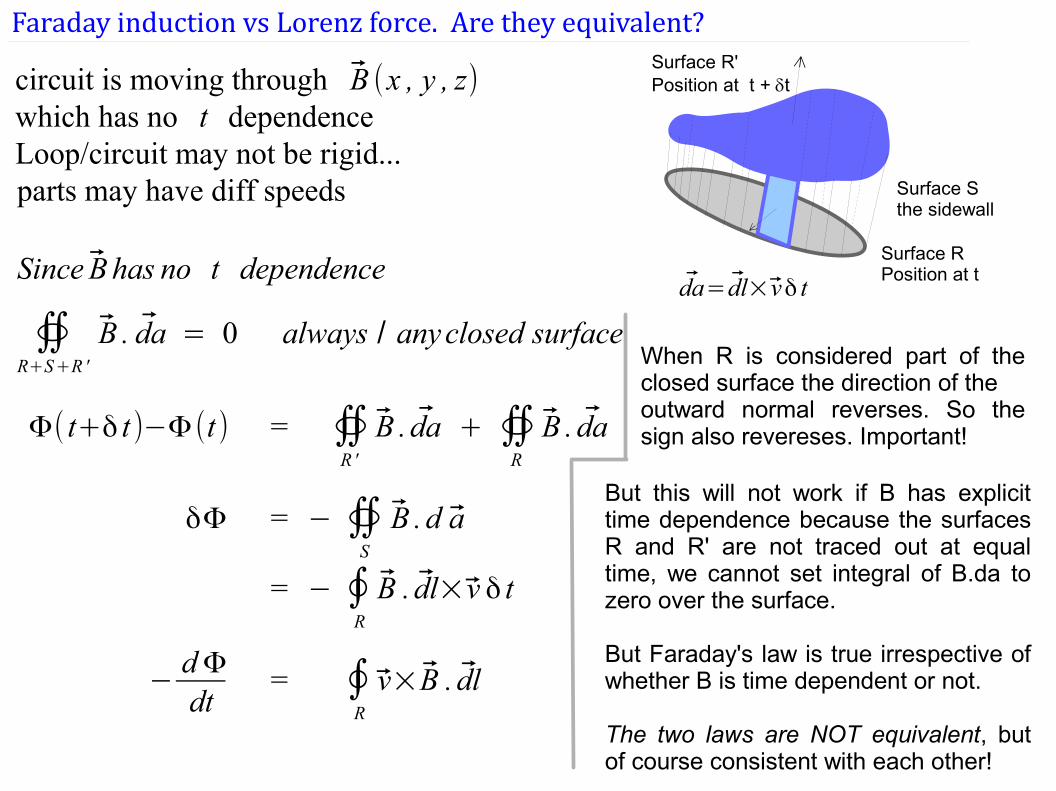
Faraday induction vs Lorenz force. Are they equivalent?
Surface RPosition at t
Surface R'Position at t + dt
da= dl× vδ t
Surface Sthe sidewall
circuit is moving through B (x , y , z)which has no t dependenceLoop/circuit may not be rigid...parts may have diff speeds
Since B has no t dependence
∯R+S+R'
B . da = 0 always / anyclosed surface
Φ( t+δ t)−Φ(t) = ∯R'
B . da + ∯R
B . da
δΦ = − ∯S
B . d a
= − ∮R
B . dl× v δ t
−dΦdt
= ∮R
v×B . dl
When R is considered part of the closed surface the direction of the outward normal reverses. So the sign also revereses. Important!
But this will not work if B has explicit time dependence because the surfaces R and R' are not traced out at equal time, we cannot set integral of B.da to zero over the surface.
But Faraday's law is true irrespective of whether B is time dependent or not.
The two laws are NOT equivalent, but of course consistent with each other!
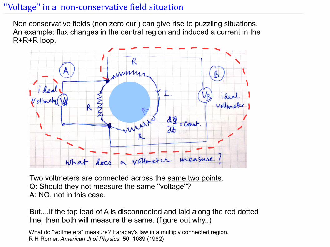
''Voltage'' in a non-conservative field situation
Two voltmeters are connected across the same two points.Q: Should they not measure the same ''voltage''?A: NO, not in this case.
But....if the top lead of A is disconnected and laid along the red dotted line, then both will measure the same. (figure out why..)
What do ''voltmeters'' measure? Faraday's law in a multiply connected region.R H Romer, American Jl of Physics 50, 1089 (1982)
Non conservative fields (non zero curl) can give rise to puzzling situations. An example: flux changes in the central region and induced a current in the R+R+R loop.
Energy and Momentum of particle + EM field system
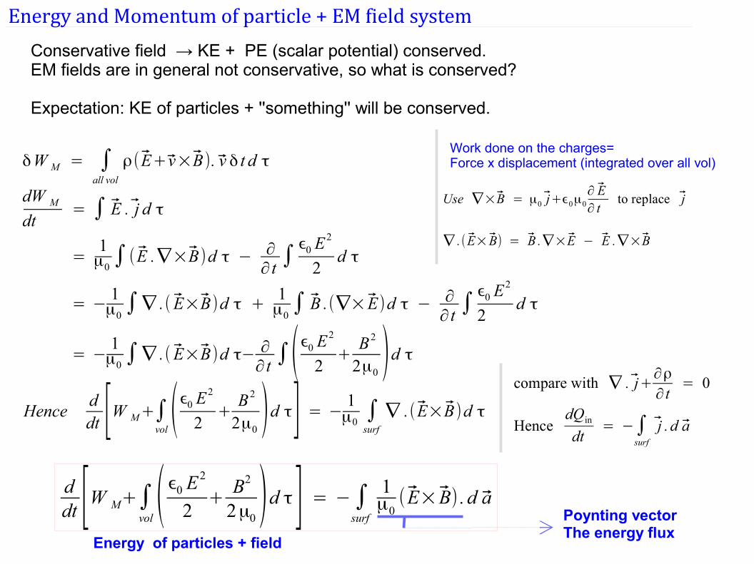
Conservative field → KE + PE (scalar potential) conserved.EM fields are in general not conservative, so what is conserved?
Expectation: KE of particles + ''something'' will be conserved.
δW M = ∫all vol
ρ( E+ v×B). v δ t d τ
dW M
dt= ∫ E . j d τ
=1μ0∫( E .∇×B)d τ − ∂
∂ t∫ϵ0 E
2
2d τ
= −1μ0∫∇ .( E×B)d τ +
1μ0∫ B .(∇× E)d τ − ∂
∂ t∫ϵ0 E
2
2d τ
= −1μ0∫∇ .( E×B)d τ− ∂
∂ t∫(ϵ0 E
2
2+
B2
2μ0)d τ
Henceddt [W M+∫
vol(ϵ0 E
2
2+B2
2μ0)d τ] = −
1μ0∫surf
∇ .( E×B)d τ
Work done on the charges=Force x displacement (integrated over all vol)
Use ∇×B = μ0 j+ϵ0μ0
∂ E∂ t
to replace j
∇ .( E× B) = B .∇×E − E .∇×B
compare with ∇ . j+∂ρ
∂ t= 0
HencedQin
dt= −∫
surf
j . d a
ddt [W M+∫
vol( ϵ0 E
2
2+
B2
2μ0)d τ ] = −∫
surf
1μ0( E× B) . d a
Poynting vectorThe energy flux
Energy of particles + field
Energy and Momentum of particle + EM field system
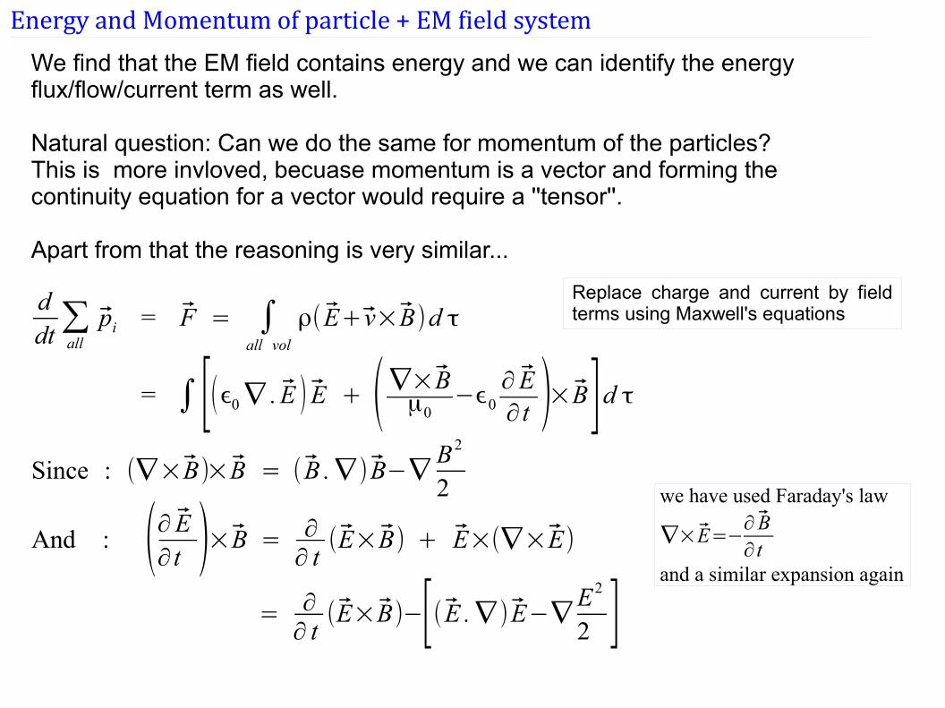
We find that the EM field contains energy and we can identify the energy flux/flow/current term as well.
Natural question: Can we do the same for momentum of the particles? This is more invloved, becuase momentum is a vector and forming the continuity equation for a vector would require a ''tensor''.
Apart from that the reasoning is very similar...
ddt∑all
pi = F = ∫all vol
ρ( E+ v×B)d τ
= ∫[(ϵ0∇ . E ) E + (∇×Bμ0−ϵ0
∂ E∂ t )×B]d τ
Since : (∇×B)×B = ( B .∇) B−∇B2
2
And : (∂ E∂ t )×B = ∂∂ t(E×B) + E×(∇×E)
= ∂∂ t(E×B)−[( E .∇) E−∇ E2
2 ]
Replace charge and current by field terms using Maxwell's equations
we have used Faraday's law
∇×E=−∂ B∂ t
and a similar expansion again
Energy and Momentum of particle + EM field system
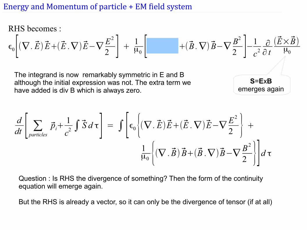
RHS becomes :
ϵ0[(∇ . E) E+( E .∇) E−∇E2
2 ] + 1μ0 [(∇ . B) B+( B .∇) B−∇
B2
2 ]−1
c2∂∂ t(E×B)μ0
The integrand is now remarkably symmetric in E and B although the initial expression was not. The extra term we have added is div B which is always zero.
S=ExB emerges again
ddt [ ∑particles pi+
1
c2 ∫ S d τ] = ∫[ϵ0{(∇ . E) E+(E .∇) E−∇E2
2 } +1μ0 {(∇ . B) B+(B .∇) B−∇
B2
2 }]d τQuestion : Is RHS the divergence of something? Then the form of the continuity equation will emerge again.
But the RHS is already a vector, so it can only be the divergence of tensor (if at all)
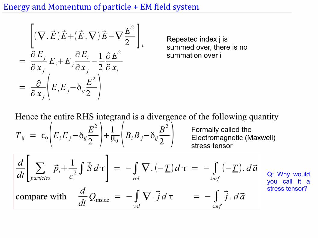
Energy and Momentum of particle + EM field system
[(∇ . E ) E+( E .∇) E−∇E2
2 ] i=∂ E j
∂ x j
E i+E j
∂Ei
∂ x j
−12∂E2
∂ xi
= ∂∂ x j(E iE j−δ ij
E2
2 )Hence the entire RHS integrand is a divergence of the following quantity
T ij = ϵ0(E iE j−δijE2
2 )+1μ0 (BiB j−δij
B2
2 )
Repeated index j is summed over, there is no summation over i
Formally called theElectromagnetic (Maxwell) stress tensor
ddt [ ∑particles pi+
1
c2∫ S d τ] = −∫vol
∇ . (−T )d τ = −∫surf
(−T ) . d a
compare withddtQinside = −∫
vol
∇ . j d τ = −∫surf
j . d a
Q: Why would you call it a stress tensor?
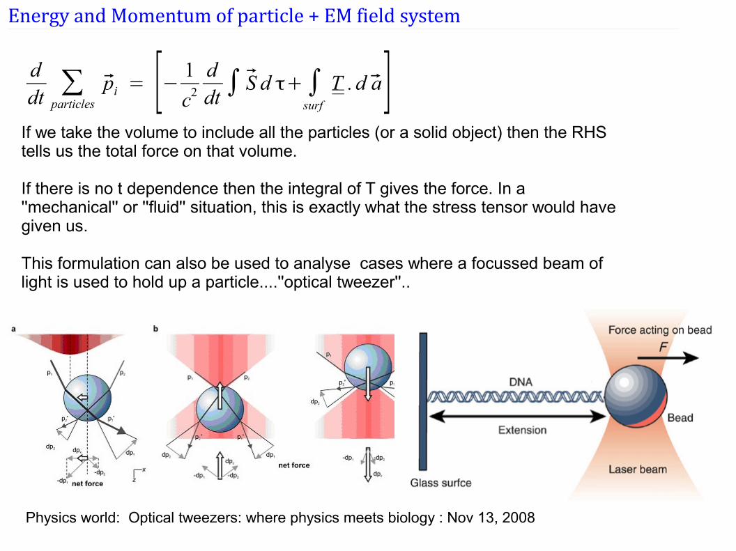
Energy and Momentum of particle + EM field system
ddt∑
particles
pi = [− 1
c2
ddt∫ S d τ+∫
surf
T .d a]If we take the volume to include all the particles (or a solid object) then the RHS tells us the total force on that volume.
If there is no t dependence then the integral of T gives the force. In a ''mechanical'' or ''fluid'' situation, this is exactly what the stress tensor would have given us.
This formulation can also be used to analyse cases where a focussed beam of light is used to hold up a particle....''optical tweezer''..
Physics world: Optical tweezers: where physics meets biology : Nov 13, 2008
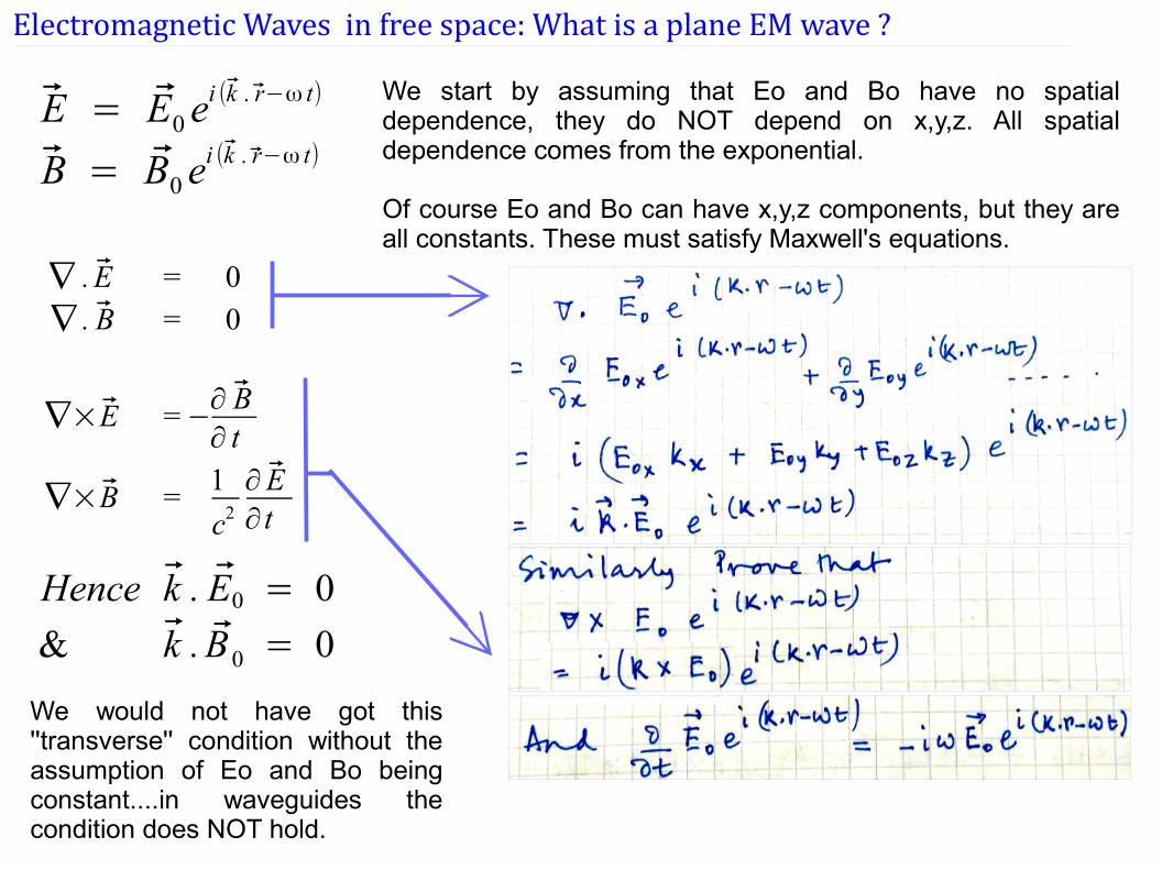
Electromagnetic Waves in free space: What is a plane EM wave ?
E = E0 ei (k . r−ω t)
B = B0 ei (k . r−ω t)
We start by assuming that Eo and Bo have no spatial dependence, they do NOT depend on x,y,z. All spatial dependence comes from the exponential.
Of course Eo and Bo can have x,y,z components, but they are all constants. These must satisfy Maxwell's equations.
∇ . E = 0∇ . B = 0
∇×E =−∂ B∂ t
∇×B =1
c2
∂ E∂ t
Hence k . E0 = 0
& k . B0 = 0
We would not have got this ''transverse'' condition without the assumption of Eo and Bo being constant....in waveguides the condition does NOT hold.
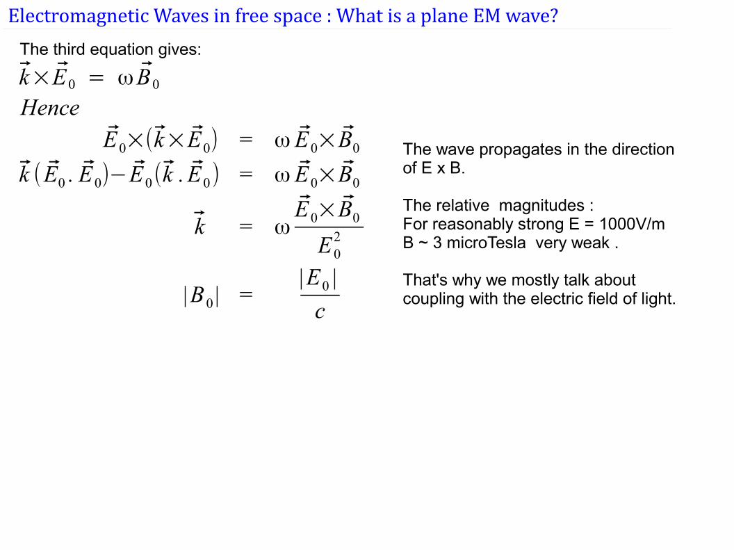
Electromagnetic Waves in free space : What is a plane EM wave?
k×E0 = ω B0
HenceE0×(k×E0) = ω E0×B0
k ( E0 . E0)−E0(k . E0) = ω E0×B0
k = ωE0×B0
E02
|B0 | =|E0 |
c
The third equation gives:
The wave propagates in the direction of E x B.
The relative magnitudes :For reasonably strong E = 1000V/m B ~ 3 microTesla very weak .
That's why we mostly talk about coupling with the electric field of light.
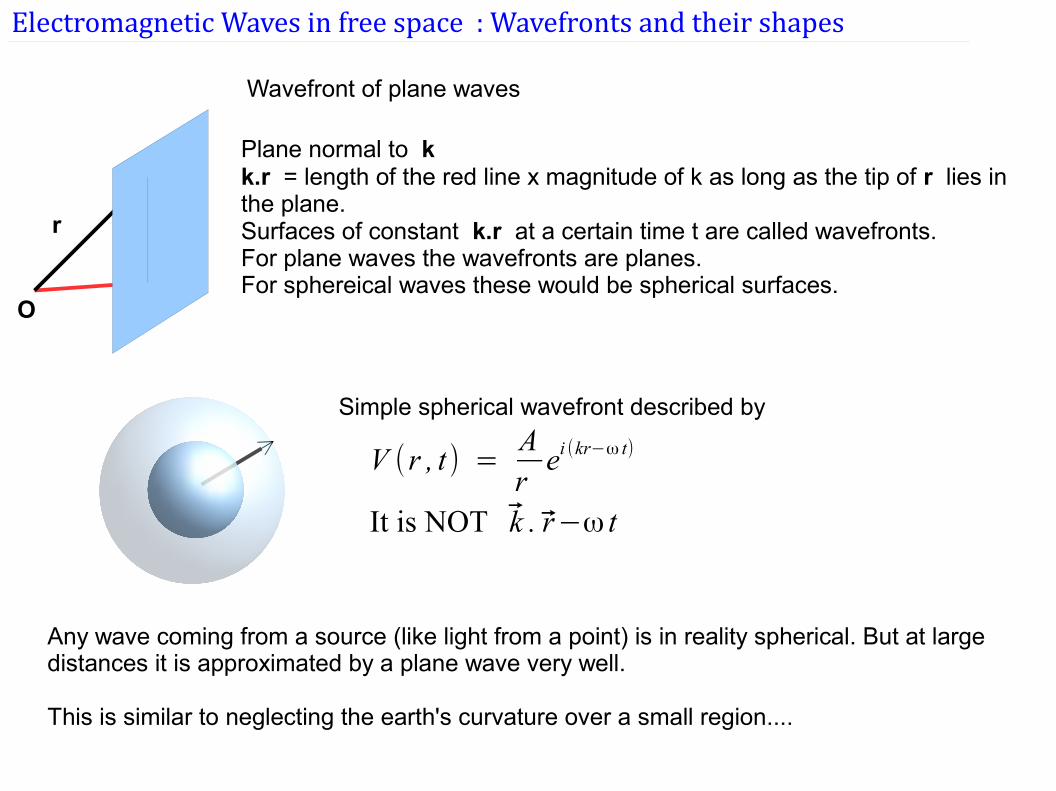
V (r , t) =Arei (kr−ω t)
It is NOT k . r−ω t
Simple spherical wavefront described by
O
r
Plane normal to kk.r = length of the red line x magnitude of k as long as the tip of r lies in the plane.Surfaces of constant k.r at a certain time t are called wavefronts.For plane waves the wavefronts are planes. For sphereical waves these would be spherical surfaces.
Electromagnetic Waves in free space : Wavefronts and their shapes
Wavefront of plane waves
Any wave coming from a source (like light from a point) is in reality spherical. But at large distances it is approximated by a plane wave very well.
This is similar to neglecting the earth's curvature over a small region....
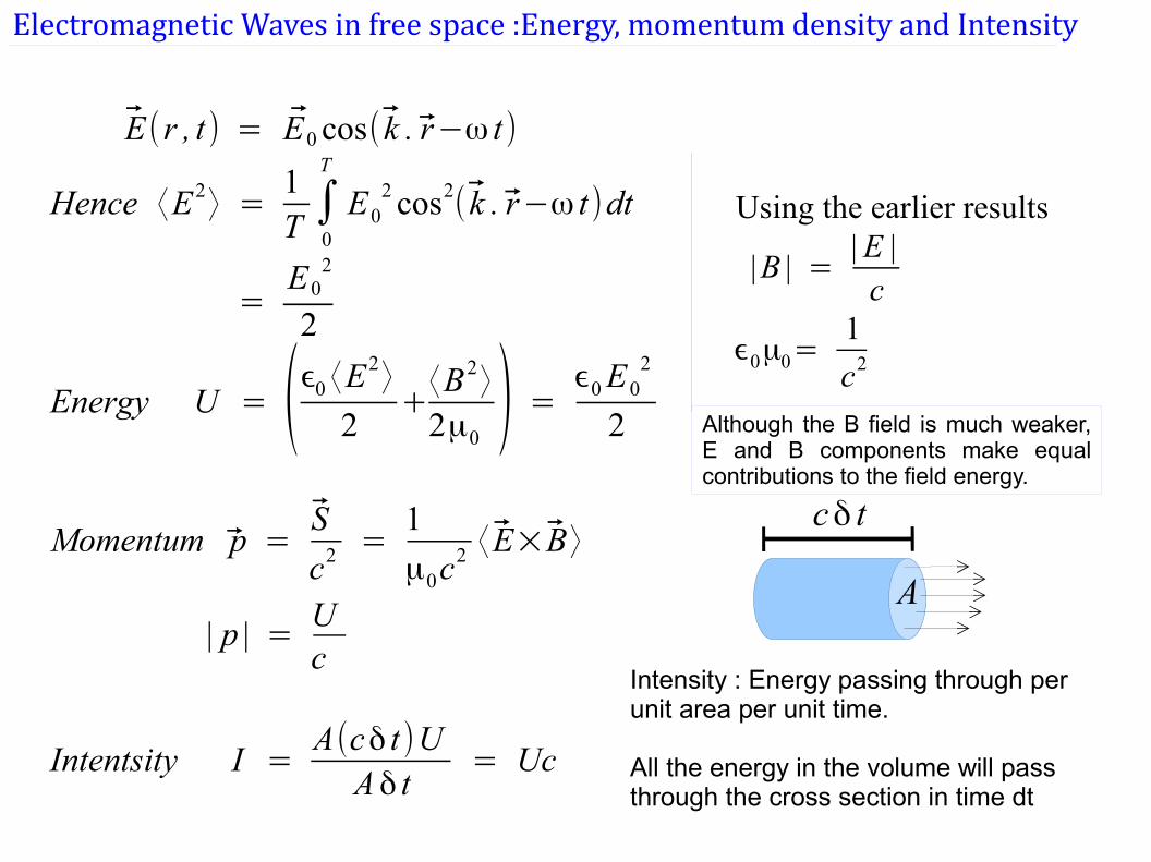
Electromagnetic Waves in free space :Energy, momentum density and Intensity
E(r , t) = E0 cos( k . r−ω t)
Hence ⟨E2⟩ =
1T∫0
T
E02 cos2
( k . r−ω t)dt
=E0
2
2
Energy U = (ϵ0 ⟨E2⟩
2+⟨B2
⟩
2μ0) = ϵ0E0
2
2
Momentum p =S
c2 =1
μ0c2 ⟨ E×B⟩
| p | =Uc
Intentsity I =A(cδ t)UAδ t
= Uc
Using the earlier results
|B | =|E |c
ϵ0μ0=1
c2
Intensity : Energy passing through per unit area per unit time.
All the energy in the volume will pass through the cross section in time dt
cδ t
A
Although the B field is much weaker, E and B components make equal contributions to the field energy.
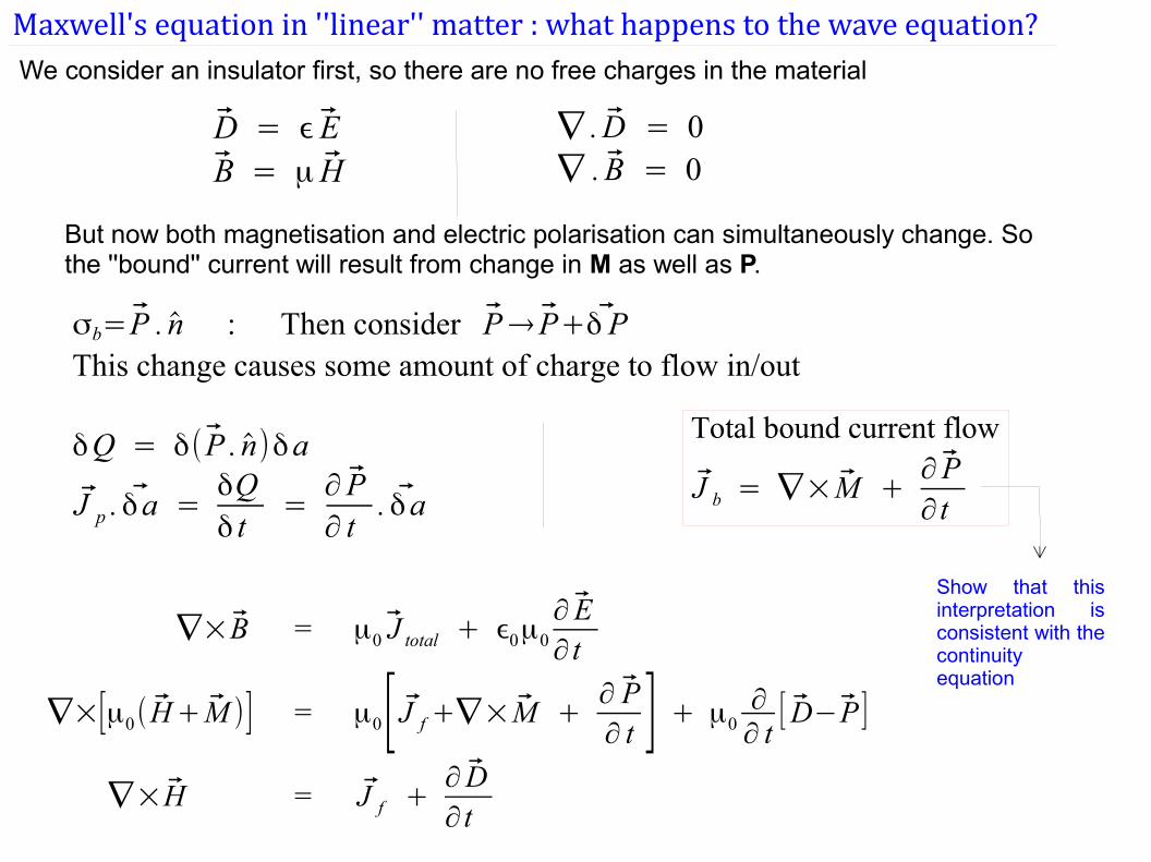
Maxwell's equation in ''linear'' matter : what happens to the wave equation?We consider an insulator first, so there are no free charges in the material
D = ϵ EB = μ H
∇ . D = 0∇ . B = 0
But now both magnetisation and electric polarisation can simultaneously change. So the ''bound'' current will result from change in M as well as P.
σb=P . n : Then consider P→ P+δ PThis change causes some amount of charge to flow in/out
δQ = δ( P . n)δa
J p . δa =δQδ t
=∂ P∂ t
. δa
Total bound current flow
J b = ∇×M +∂ P∂ t
∇×B = μ0 J total + ϵ0μ0
∂ E∂ t
∇×[μ0(H+M )] = μ0[ J f+∇×M +∂ P∂ t ] + μ0
∂∂ t
[ D−P ]
∇×H = J f +∂ D∂ t
Show that this interpretation is consistent with the continuity equation
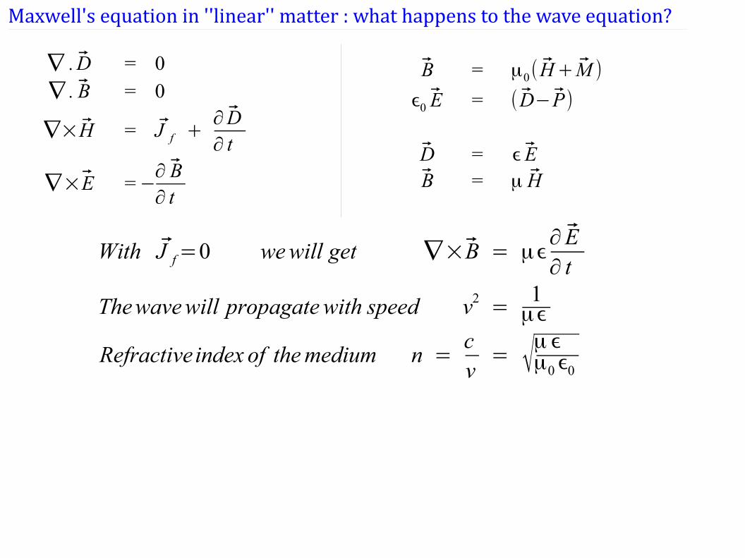
Maxwell's equation in ''linear'' matter : what happens to the wave equation?
∇ . D = 0∇ . B = 0
∇×H = J f +∂ D∂ t
∇×E =−∂ B∂ t
B = μ0(H+M )
ϵ0 E = (D−P)
D = ϵ EB = μ H
With J f=0 wewill get ∇×B = μϵ∂ E∂ t
Thewavewill propagatewith speed v2=
1μϵ
Refractiveindex of themedium n =cv= √
μ ϵμ0ϵ0
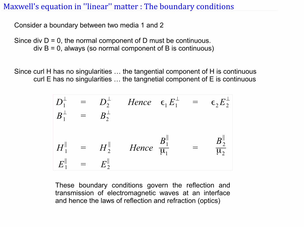
Maxwell's equation in ''linear'' matter : The boundary conditions
Consider a boundary between two media 1 and 2
Since div D = 0, the normal component of D must be continuous. div B = 0, always (so normal component of B is continuous)
Since curl H has no singularities … the tangential component of H is continuous curl E has no singularities … the tangnetial component of E is continuous
D1⊥ = D2
⊥ Hence ϵ1 E1⊥ = ϵ2E2
⊥
B1⊥ = B2
⊥
H 1∥ = H 2
∥ HenceB1∥
μ1=
B2∥
μ2
E1∥ = E2
∥
These boundary conditions govern the reflection and transmission of electromagnetic waves at an interface and hence the laws of reflection and refraction (optics)
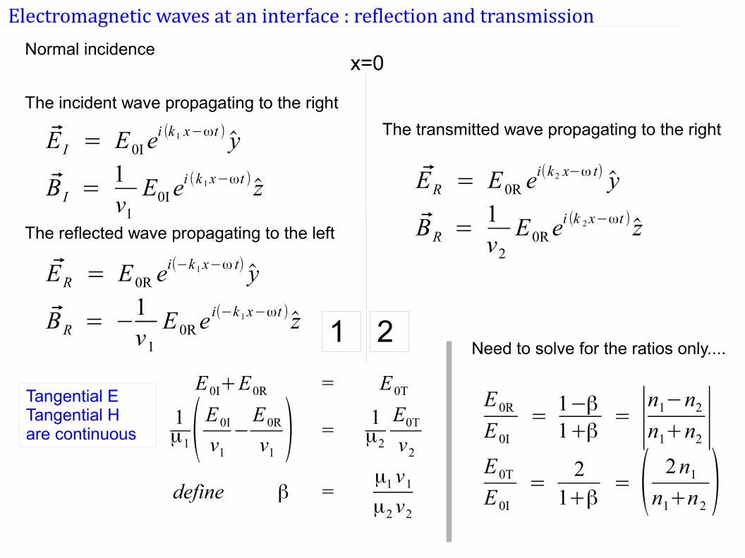
Electromagnetic waves at an interface : reflection and transmission
E I = E0Iei (k1 x−ωt ) y
B I =1v1
E0Iei (k1x−ωt ) z
The incident wave propagating to the right
The reflected wave propagating to the left
Normal incidence
ER = E0R ei(−k1x−ω t) y
BR = −1v1
E0Rei(−k1x−ωt ) z
ER = E0R ei(k2 x−ω t) y
BR =1v2
E0Rei (k 2x−ωt ) z
The transmitted wave propagating to the right
1 2
x=0
E0I+E0R = E0T
1μ1( E0I
v1
−E0R
v1) =
1μ2
E0T
v2
define β =μ1 v1
μ2 v2
Tangential ETangential Hare continuous
E0R
E0I
=1−β1+β
= ∣n1−n2
n1+n2 ∣E0T
E0I
=2
1+β= ( 2n1
n1+n2)
Need to solve for the ratios only....
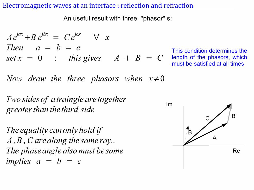
Electromagnetic waves at an interface : reflection and refraction
An useful result with three ''phasor'' s:
Aeiax+B eibx = Ceicx ∀ xThen a = b = cset x = 0 : this gives A + B = C
Now draw the three phasors when x≠0
Two sides of a traingle are togethergreater than thethird side
Theequality canonly hold ifA ,B ,C arealong the same ray..The phaseangle alsomust be sameimplies a = b = c
Re
Im
A
BC
This condition determines the length of the phasors, which must be satisfied at all times
B
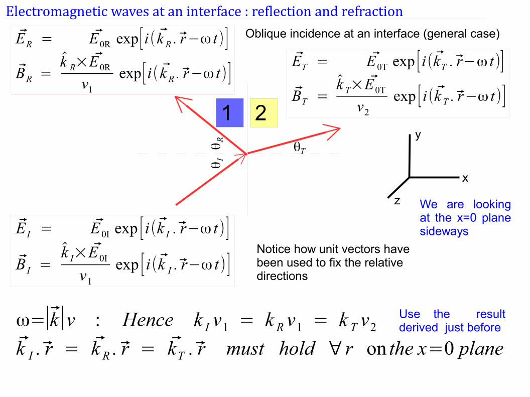
Electromagnetic waves at an interface : reflection and refractionOblique incidence at an interface (general case)
1 2
θIθR
θT
E I = E0I exp [i(k I . r−ω t)]
B I =k I×E0I
v1
exp [i(k I . r−ω t)]
ER = E0R exp[i( k R . r−ω t)]
BR =k R×E0R
v1
exp[i( k R . r−ω t)]ET = E0T exp [i(kT . r−ω t)]
BT =k T×E0T
v2
exp [i(k T . r−ω t)]
Notice how unit vectors have been used to fix the relative directions
x
y
z We are looking at the x=0 plane sideways
ω=∣k∣v : Hence k I v1 = k R v1 = k T v2
k I . r = k R . r = kT . r must hold ∀r on the x=0 plane
Use the result derived just before
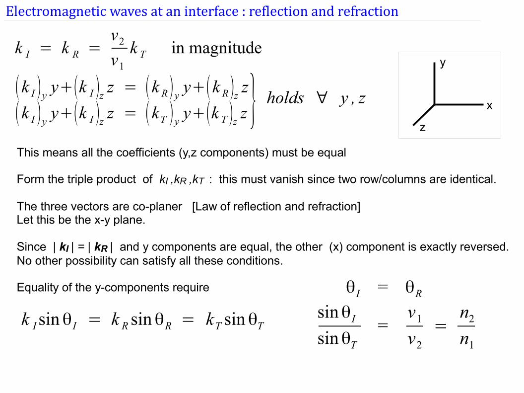
Electromagnetic waves at an interface : reflection and refraction
k I = k R =v2
v1
k T in magnitude
(k I )y y+(k I )z z = (k R)y y+(k R)z z(k I )y y+(k I )z z = (kT )y y+(k T )z z} holds ∀ y , z x
y
z
This means all the coefficients (y,z components) must be equal
Form the triple product of kI ,kR ,kT : this must vanish since two row/columns are identical.
The three vectors are co-planer [Law of reflection and refraction]Let this be the x-y plane.
Since | kI | = | kR | and y components are equal, the other (x) component is exactly reversed.No other possibility can satisfy all these conditions.
Equality of the y-components require
k IsinθI = k R sinθR = kT sinθT
θI = θRsinθIsinθT
=v1
v2
=n2
n1